Finite Element Analysis of the Modified Ring Test for ...jte2/references/link115.pdf ·...

Pergamon Int. J. Rock Mech. Min. Sci. & Geomech. Abstr. Vol. 33, No. 1, pp. 1-15, 1996

Copyright © 1996 Elsevier Science Ltd 0148-9062(95)00043-7 Printed in Great Britain. All rights reserved

0148-9062/96 $15.00 + 0.00

Finite Element Analysis of the Modified Ring Test for Determining Mode I Fracture Toughness M.P. FISCHER?~ D. ELSWORTH§ R.B. ALLEY~ T. ENGELDER¶

Plane strain fracture toughness (Klc) values are determined for the modified ring (MR) test through numerical simulation of crack growth to highlight the sensitivity of MR Ktc values on applied displacement or force boundary conditions, slip conditions at the specimen-platen interface, and the Poisson ratio (v) of the test material. Numerical calculation of fracture toughness in the MR test is traditionally conducted assuming a uniform force along the specimen loading surfaces and no slip between the specimen and the loading platens. Under these conditions K+c increases by 30-40% as v decreases from 0.4 to O. 1. When slip is allowed at the specimen-platen interface under a uniform force, Kic values are independent of v, and for any given v, are 5-25% less than those determined under a no-slip boundary condition. Under a uniform displacement of the specimen loading surfaces, K+, is essentially independent of v, regardless of specimen-platen interaction. Moreover, although K+c values determined under uniform displacement and no-slip boundary conditions are always higher than those determined under uniform displacement and slip-allowed boundary conditions, the average difference in Klc for these two methods is less than 5% for the two specimen geometries examined. This suggests that under uniform displacement conditions, Ku is essentially independent of specimen-platen interaction. Because KIc values determined from MR testing are strongly dependent on the modeling procedure, future reports of KI~ determined from this test should be accompanied by detailed reports of the modeling procedure. Until further testing reveals the most accurate simulation technique, we advocate use of a uniform displacement formulation for K~ determination from MR testing because results from this method are insensitive to most modeling parameters. Numerical results from models conducted under uniform force, no -slip boundary conditions should be viewed as an upper bound to KI~.

INTRODUCTION

The modified ring (MR) test for plane strain fracture toughness determination involves two phases: laboratory deformation of a specimen, and numerical calcu-

tTo whom all correspondence should be addressed at: Department of Geology, Northern Illinois University, DeKalb, IL 60115-2854, U.S.A.

:IDepartment of Geosciences and Earth System Science Center, The Pennsylvania State University, University Park, PA 16802, U.S.A.

§Department of Mineral Engineering, The Pennsylvania State University, University Park, PA 16802, U.S.A.

¶Department of Geoseiences, The Pennsylvania State University, University Park, PA 16802, U.S.A.

lation of crack-tip stress intensity factors in a model with exactly the same dimensions as the laboratory specimen [1]. Published results using the modified ring test have utilized displacement discontinuity [1] and finite element [2-4] techniques for the second phase of the test, but do not provide detailed descriptions of the modeling procedure. This paper is concerned with the parameters that affect the numerical modeling results for MR tests on unconfined specimens, specifically when the modeling is accomplished using the finite element method.

In the first phase of the MR test, two diametrically opposed, flat loading surfaces are machined along the

2 FISCHER e t al.: MODE I FRACTURE TOUGHNESS

(a) F ' ~

/ / / ~ t

I ', 2a l l ) \::: ,r- '" /

(b) F ' ~

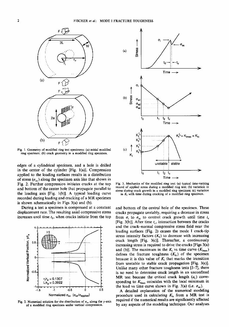
Fig. I. Geometry of modified ring test specimens: (a) initial modified ring specimen; (b) crack geometry in a modified ring specimen.

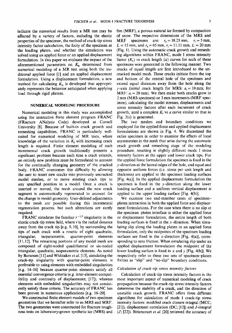
edges of a cylindrical specimen, and a hole is drilled in the center of the cylinder [Fig. l(a)]. Compression applied to the loading surfaces results in a distribution of stress (axx) along the specimen axis like that shown in Fig. 2. Further compression initiates cracks at the top and bottom of the center hole that propagate parallel to the loading axis [Fig. l(b)]. A typical loading curve recorded during loading and cracking of a MR specimen is shown schematically in Figs 3(a) and (b).

During a test a specimen is compressed at a constant displacement rate. The resulting axial compressive stress increases until time to, when cracks initiate from the top

t , = I i I i i i i i | i , 1 , i t i

o.

.-~ 0- ..................................................... ~ ............................ I . . . . . . . . . . . . . . . . . . . . . . . . . . .

" i

o. . - i

-0.5 ............................. i ........................... ~ . . . . . . . . . . . . . . . . . . . . .

"~ ri/r e = 0.1307 z k/r e = 0.3922

-1.5 -1 -0.5 0.5

Normalized Oxx (Oxx/Gapplied) Fig. 2. Numerical solution for the distribution of G,~ along the y-axis

of a modified ring specimen under vertical compression.

(a)

T (b) ,~

T u) ¢/)

(3al

q3a2 ( ~ a c

O i

il--

Time >

to tl t2 tc Time >

f

) ,

t t KI c

K~ 2

(c) T K~I K~ 0, Ki

to

~ = Klmax

q l I=

unstable stable

tl t2 tc

Time >

= Kle

Fig. 3. Mechanics of the modified ring test: (a) typical time-varying record of applied stress during a modified ring test; (b) variation in stress during crack growth in a modified ring specimen; (c) variation

in K t with time during cracking of a modified ring specimen.

and bottom of the central hole of the specimen. These cracks propagate unstably, requiring a decrease in stress from a~ to a,c to control crack growth until time t¢ [Fig. 3(b)]. After time re, interaction between the cracks and the crack-normal compressive stress field near the loading surfaces (Fig. 2) causes the mode I crack-tip stress intensity factors (K~) to decrease with increasing crack length [Fig. 3(c)]. Thereafter, a continuously increasing stress is required to drive the cracks [Figs 3(a) and (b)]. The maximum in the Kl vs time curve (Kim~) defines the fracture toughness (Kit) of the specimen because it is this value of KI that marks the transition from unstable to stable crack propagation [Fig. 3(¢)]. Unlike many other fracture toughness tests [5-7], there is no need to determine crack length in an unconfined MR test because the critical crack length (ac) corresponding to Kxm.x coincides with the local minimum in the load vs time curve shown in Fig. 3(a) (i.e. trio).

A detailed explanation of the numerical modeling procedure used in calculating Kxo from a MR test is required if the numerical results are significantly affected by any aspects of the modeling technique. Our analyses

FISCHER et al.: MODE I FRACTURE TOUGHNESS 3

indicate the numerical results from a MR test may be affected by a variety of factors, including the elastic properties of the specimen, the method of crack-tip stress intensity factor calculation, the fixity of the specimen at the loading platen, and whether the simulation was solved using an applied force or an applied displacement formulation. In this paper we evaluate the impact of the aforementioned parameters on K~c determined from numerical modeling of a MR test using both the traditional applied force [1] and an applied displacement formulation. Using a displacement formulation, a new method for calculating K~c is developed that appropri- ately represents the behavior anticipated when applying load through rigid platens.

NUMERICAL MODELING PROCEDURE

Numerical modeling in this study was accomplished using the interactive finite element program FRANC (FRacture ANalysis Code) developed at Cornell University [8]. Because of built-in crack growth and remeshing capabilities, FRANC is particularly well- suited for numerical modeling of MR tests, where knowledge of the variation in K~ with increasing crack length is required. Finite element modeling of such incremental crack growth traditionally presents a significant problem because each time a crack extends, an entirely new problem must be formulated to account for the continually changing geometry of the cracked body. FRANC overcomes this difficulty by allowing the user to insert new cracks into previously uncracked model meshes, or to move existing crack tips to any specified position in a model. Once a crack is inserted or moved, the mesh around the new crack segment is automatically regenerated to account for the change in model geometry. User-defined adjustments to the mesh are possible during this incremental regeneration process, but such alterations are rarely required.

FRANC simulates the familiar r - 1/2 singularity in the elastic crack-tip stress field, where r is the radial distance away from the crack tip [e.g. 9, 10], by surrounding the tips of each crack with a rosette of eight quadratic, triangular, isoparametric, quarter-point elements [11, 12]. The remaining portions of any model mesh are composed of eight-noded quadrilateral or six-noded triangular, quadratic, isoparametric elements. As noted by Barsoum [11] and Whittaker et al. [13], simulating the crack-tip singularity with quarter-point elements is preferable to using elements with embedded singularities [e.g. 14-16] because quarter-point elements satisfy all essential convergence criteria (e.g. inter-element compat- ibility and continuity of displacement; [17]), whereas elements with embedded singularities may not consist- ently satisfy these criteria. The accuracy of FRANC has been proven in numerous applications [e.g. 18-20].

We constructed finite element models of two specimen geometries that we hereafter refer to as MRS and MRF. The two geometries were constructed for fracture toughness tests on laboratory-grown synthetic ice (MRS) and

firn (MRF), a porous natural ice formed by compaction of snow. The respective dimensions of the MRS and MRF specimens are: re=38.25mm, r~=5mm, L = 15 mm, and re = 65 mm, r i = 11.11 mm, L = 20 mm (Fig. 1). Using the automatic crack growth and remeshing algorithms within FRANC, mode I stress intensity factor (K~) vs crack length (a) curves for each of these specimens were generated in the following manner. Two cracks of equal length are first introduced to the uncracked model mesh. These cracks initiate from the top and bottom of the central hole of the specimen and extend equal distances away from the hole along the y-axis (initial crack length for MRS: ai = 10mm; for MRF: ai = 20 mm). We then make both cracks grow in 2 mm (MRS specimen) or 3 mm increments (MRF specimen), calculating the model stresses, displacements and stress intensity factors after each increment of crack growth, until a complete KI vs a curve similar to that in Fig. 3(c) is generated.

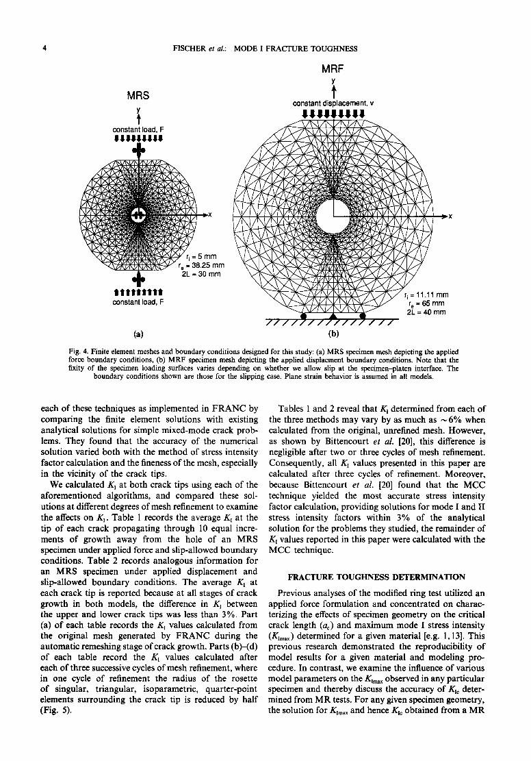
The two meshes and boundary conditions we employed for the applied force and applied displacement formulations are shown in Fig. 4. We discretized the entire specimen in order to examine the effects of local asymmetries in the mesh that arise during the automatic crack growth and remeshing stage of the modeling procedure, resulting in slightly different mode I stress intensity factors at the upper and lower crack tips. For the applied force formulation the specimen is fixed in the y-direction at the lateral edges of the hole, and equal and opposite uniform forces (i.e. stress per unit length and thickness) are applied to the specimen loading surfaces [Fig. 4(a)]. In the applied displacement formulation the specimen is fixed in the y-direction along the lower loading surface and a uniform vertical displacement is applied to the upper loading surface [Fig. 4(b)].

We examine two end-member cases of specimen- platen interaction in both the applied force and displacement formulations. For the case when there is no slip at the specimen-platen interface in either the applied force or displacement formulation, the entire length of both loading surfaces is fixed in the x-direction. When simulating slip along the loading platen in an applied force formulation, only the midpoints of the specimen loading surfaces are fixed in the x-direction [Fig. 4(a)], corresponding to zero friction. When simulating slip under an applied displacement formulation the midpoint of the lower loading surface is fixed in x and y [Fig. 4(b)]. We respectively refer to these two sets of specimen-platen fixities as "slip" and "no-slip" boundary conditions.

Calculation o f crack-tip stress intensity factors

Calculation of crack-tip stress intensity factors is the most important aspect of numerical modeling of crack propagation because the crack-tip stress intensity factors determine the stability of a crack, and the direction of unstable crack growth. FRANC offers three different algorithms for calculation of mode I crack-tip stress intensity factors: modified crack closure integral (MCC; [21]), displacement correlation (DC; [12]) and J-integral (J; [22]). Bittencourt et al. [20] reviewed the accuracy of

4 FISCHER et al.: MODE I FRACTURE TOUGHNESS

MRS

constant load, F l l l l i l l i l +

~X

5 mm .25 mm

2L = 30 mm

t t t t t t t t t constant load, F

MRF Y

t constant displacement, v

l l l l l l i l l

(a) (b)

Fig. 4. Finite element meshes and boundary conditions designed for this study: (a) MRS specimen mesh depicting the applied force boundary conditions, (b) MRF specimen mesh depicting the applied displacment boundary conditions. Note that the fixity of the specimen loading surfaces varies depending on whether we allow slip at the specimen-platen interface. The

boundary conditions shown are those for the slipping case. Plane strain behavior is assumed in all models.

each of these techniques as implemented in FRANC by comparing the finite element solutions with existing analytical solutions for simple mixed-mode crack problems. They found that the accuracy of the numerical solution varied both with the method of stress intensity factor calculation and the fineness of the mesh, especially in the vicinity of the crack tips.

We calculated K~ at both crack tips using each of the aforementioned algorithms, and compared these solutions at different degrees of mesh refinement to examine the affects on K~. Table 1 records the average K~ at the tip of each crack propagating through 10 equal increments of growth away from the hole of an MRS specimen under applied force and slip-allowed boundary conditions. Table 2 records analogous information for an MRS specimen under applied displacement and slip-allowed boundary conditions. The average K~ at each crack tip is reported because at all stages of crack growth in both models, the difference in K~ between the upper and lower crack tips was less than 3%. Part (a) of each table records the Kt values calculated from the original mesh generated by FRANC during the automatic remeshing stage of crack growth. Parts (b)-(d) of each table record the Kx values calculated after each of three successive cycles of mesh refinement, where in one cycle of refinement the radius of the rosette of singular, triangular, isoparametric, quarter-point elements surrounding the crack tip is reduced by half (Fig. 5).

Tables 1 and 2 reveal that K~ determined from each of the three methods may vary by as much as ,-, 6% when calculated from the original, unrefined mesh. However, as shown by Bittencourt e t al. [20], this difference is negligible after two or three cycles of mesh refinement. Consequently, all Kt values presented in this paper are calculated after three cycles of refinement. Moreover, because Bittencourt e t al. [20] found that the MCC technique yielded the most accurate stress intensity factor calculation, providing solutions for mode I and II stress intensity factors within 3% of the analytical solution for the problems they studied, the remainder of KI values reported in this paper were calculated with the MCC technique.

FRACTURE TOUGHNESS DETERMINATION

Previous analyses of the modified ring test utilized an applied force formulation and concentrated on charac- terizing the effects of specimen geometry on the critical crack length (ac) and maximum mode I stress intensity (Klmax) determined for a given material [e.g. l, 13]. This previous research demonstrated the reproducibility of model results for a given material and modeling procedure. In contrast, we examine the influence of various model parameters on the Kimax observed in any particular specimen and thereby discuss the accuracy of Ktc determined from MR tests. For any given specimen geometry, the solution for Ktm,x and hence K=¢ obtained from a MR

FISCHER et al.: M O D E I F R A C T U R E T O U G H N E S S 5

Table 1. Effects of mesh refinement and method of calculation on the mode I stress intensity factor determined under constant force and slip-allowed boundary conditions for a modified ring specimen with normalized dimensions: ri/r~ = 0.1307 and L/ro = 0.3992. In this model, Young's modulus = 9 GPa, Poisson ratio = 0.32 and normal- to-the-boundary, axial stress = 2.238 MPa. Numbers in bold are the peak stress intensity factors (i.e. Kit) encountered during crack growth

Crack Length, a (mm) K l (DC) K l (MCC) K l (J)

(a) For the origmal, unrefined mesh I0 120.66 123.79 129.45 12 125.18 127.72 133.45 14 131.49 133.83 139.93 16 138.48 141.32 147.74 18 147.05 148.20 155.82 20 151.39 154.51 161.28 22 155.33 158.18 165.83 24 154.98 158.79 166.70 26 149.05 155.00 161.96 28 137.86 144.37 150.57

(b) After one cyc&ofmesh refinement 10 122.96 123.17 122.92 12 126.90 126.70 126.59 14 133.05 133.01 132.78 16 140.12 140.03 139.65 18 147.96 147.90 147.63 20 153.16 153.47 153.01 22 157.42 157.64 157.35 24 157.29 158.34 157.92 26 152.18 153.96 153.51 28 141.29 143.58 143.17

(c) After two cyc&sofmesh refinement 10 123.03 123.11 122.95 12 126.70 126.70 126.59 14 132.99 132.86 132.74 16 139.93 139.82 139.61 18 147.79 147.80 147.60 20 153.26 153.24 152.99 22 157.34 157.53 157.43 24 157.62 158.19 157.97 26 152.91 153.86 153.56 28 142.37 143.54 143.24

(d) After three cycles of mesh refinement 10 123.26 122.96 122.92 12 126.89 126.55 126.52 14 133.04 132.66 132.67 16 140.00 139.63 139.52 18 147.95 147.63 146.52 20 153.39 153.04 152.91 22 157.64 157.39 157.31 24 158.07 158.02 157.91 26 153.50 153.66 153.50 28 143.03 143.36 143.17

test under either an applied force or an applied displacement formulation depends on several model input parameters.

Applied force solution To date, the numerical modeling portion of the M R

test has been solved using an applied force formulation assuming no slip between the specimen and the loading platens [e.g. 2]. To determine the fracture toughness of a specimen under these conditions, one simply takes the value of the local load minimum recorded during a laboratory test (a J , applies an equivalent uniform stress to a sample in a numerical simulation, and calculates the K~ vs a curve corresponding to that specimen geometry and stress. The K~mx in the resulting curve is the fracture toughness of the tested material. The solution for K~c

obtained in this formulation depends on the local load minimum (trac), the behavior of the specimen-platen interface, and the Poisson ratio (v) of the test material.

Figure 6 illustrates the influence of slip at the specimen-platen interface on the K~ vs a curves obtained in an applied force formulation. All K, values are reported after three cycles of mesh refinement. Although Kt is initially greater under slip-allowed conditions, K~m~ in the no-slip case exceeds K~max for the slip-allowed case, and K~max is achieved at longer critical crack lengths under no-slip conditions. These variations in K~m~x and ac result from differences in the initial distribution of axx along the y-axis of the specimen as depicted in Fig. 7. Initial K~ values are greater under slip-allowed conditions because the maximum tensile stress near the edge of the specimen hole is greater for this situation.

Table 2. Effects of mesh refinement and method of calculation on the mode I stress intensity factor determined under constant displacement and slip-allowed boundary conditions for a modified ring specimen with normalized dimensions: r~/r~ = 0.1307 and L/r¢ = 0.3992. In this model, Young 's m o d u l u s = 9GPa , Poisson ratio =0 .32 and axial displacement = -0 .1 mm. Numbers in bold are the peak stress inten-

sity factors (i.e. K,c ) encountered during crack growth

Crack Length, a (mm) K l (DC) g~ (MCC) K l (J)

(a) Forthe origmaL unrefined mesh 10 815.56 839.74 877.69 12 817.92 837.69 874.69 14 827.72 845.60 883.86 16 834.52 855.40 893.82 18 840.54 851.60 895.08 20 810.96 833.42 869.47 22 760.37 788.19 825.83 24 688.27 714.68 749.46 26 575.54 610.48 636.42 28 439.56 475.29 493.79

(b) After one cyc& of mesh refinement 10 832.47 835.32 833.42 12 830.57 830.89 829.78 14 839.11 840.53 829.31 16 845.91 847.49 844.80 18 847.81 849.86 848.12 20 823.14 827.88 825.04 22 780.45 785.51 783.77 24 703.13 712.62 710.25 26 593.40 606.37 604.15 28 457.58 472.13 470.23

(c) After two cycles of mesh refinement 10 833.73 835.00 833.73 12 829.94 830.73 829.94 14 839.43 839.43 838.64 16 845.91 846.07 844.80 18 847.81 849.23 847.96 20 825.04 826.62 825.04 22 781.87 874.88 784.25 24 706.93 711.99 710.72 26 599.25 605.89 604.47 28 464.70 471.97 470.55

(d) After three cycles of mesh refinement 10 835.63 834.05 833.58 12 831.52 829.78 829.46 14 839.11 838.32 838.17 16 846.70 844.96 844.33 18 849.39 848.28 847.49 20 826.46 825.35 824.72 22 784.25 784.25 783.61 24 710.29 711.04 710.40 26 602.89 605.10 604.15 28 468.49 471.34 470.55


n o d e s -

original crack-tip mesh generated by FRANC

d o m a i n o f i n t e g r a t i o n

c r a c k

crack tip mesh after 2 cycles of refinement

r e f i n e m e n / ~

J

J

crack tip mesh after 1 cycle of refinement

efinement

crack tip mesh after 3 cycles of refinement

Fig. 5. Method of mesh refinement in FRANC. Note that the area utilized in calculating the ,/-integral is constant, but that the number of elements in the domain of integration increases by a factor of two during each successive refinement cycle.

However, with increasing crack length, K~ is increasingly affected by the zone of crack-normal compression near the specimen loading surfaces. Because this zone of

compression extends farther into the sample and crack-normal compressive stresses are greater in the slip- allowed case, ao is shorter and K~m~ is less in this case.

170

i 160..

1so-:

=- t3o2

,~ 12o-

110

. . . . I . . . . I L , L , I , , , L I , , , , I , , , ,

- slip ow li • 1 ~ "

............ = r e s . i E : 9 G P a ; ~) : 0 . 3 2 i i i i

. . . . . . . . i . . . . ; . . . . i . . . . i . . . . 0,2 0.3 0.4 0.5 0.6 0.7 0.8

Normalized Crack Length, a/r e

Fig. 6. Variation in KI with crack length in MRS specimen geometry as a function of specimen-platen interaction for an applied force formulation. Model material properties chosen to represent those of

granular, freshwater ice lh [see 23].

g

8 fit.

>

o Z

1- . . . . . . slip allowed ] no slip allowed ]

0.5.

-1.- I - -1.5

r/r e = O. 1307 L/r e = 0.3922

- 1 - 0 . 5

Normalized oxx (axx/aapO~d) 0.5 1

Fig. 7. Influence of specimen-platen interaction on the initial distribution of a~ along the y-axis of an MRS specimen subjected to

constant forces along the loading surfaces.


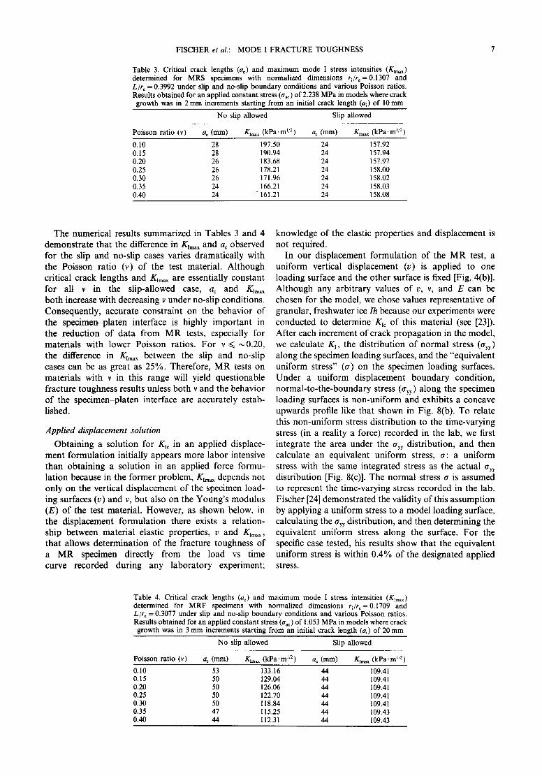
Table 3. Critical crack lengths (ac) and maximum mode I stress intensities (glmax) determined for MRS specimens with normalized dimensions r~/r~=O.1307 and L/re = 0.3992 under slip and no-slip boundary conditions and various Poisson ratios. Results obtained for an applied constant stress (c%) of 2.238 MPa in models where crack

growth was in 2mm increments starting from an initial crack length (a~) of 10mm

No slip allowed Slip allowed

Poisson ratio (v) a¢ (mm) Klm~x (kPa 'm 1/2) ac (mm) glmax (kPa 'm 1/2)

0.10 28 197.50 24 157.92 0.15 28 190.94 24 157.94 0.20 26 183.68 24 157.97 0.25 26 178.21 24 158.00 0.30 26 171.96 24 158.02 0.35 24 166.21 24 158.03 0.40 24 161.21 24 158.08

The numerical results summarized in Tables 3 and 4 demonstrate that the difference in K~max and ac observed for the slip and no-slip cases varies dramatically with the Poisson ratio (v) of the test material. Although critical crack lengths and glmax a r e essentially constant for all v in the slip-allowed case, ac and KImax both increase with decreasing v under no-slip conditions. Consequently, accurate constraint on the behavior of the specimen-platen interface is highly important in the reduction of data from MR tests, especially for materials with lower Poisson ratios. For v ~< ,-~0.20, the difference in K~max between the slip and no-slip cases can be as great as 25%. Therefore, MR tests on materials with v in this range will yield questionable fracture toughness results unless both v and the behavior of the specimen-platen interface are accurately estab- lished.

Applied displacement solution

Obtaining a solution for K~c in an applied displacement formulation initially appears more labor intensive than obtaining a solution in an applied force formulation because in the former problem, K~max depends not only on the vertical displacement of the specimen loading surfaces (v) and v, but also on the Young's modulus (E) of the test material. However, as shown below, in the displacement formulation there exists a relationship between material elastic properties, v and K~ . . . .

that allows determination of the fracture toughness of a MR specimen directly from the load vs time curve recorded during any laboratory experiment;

knowledge of the elastic properties and displacement is not required.

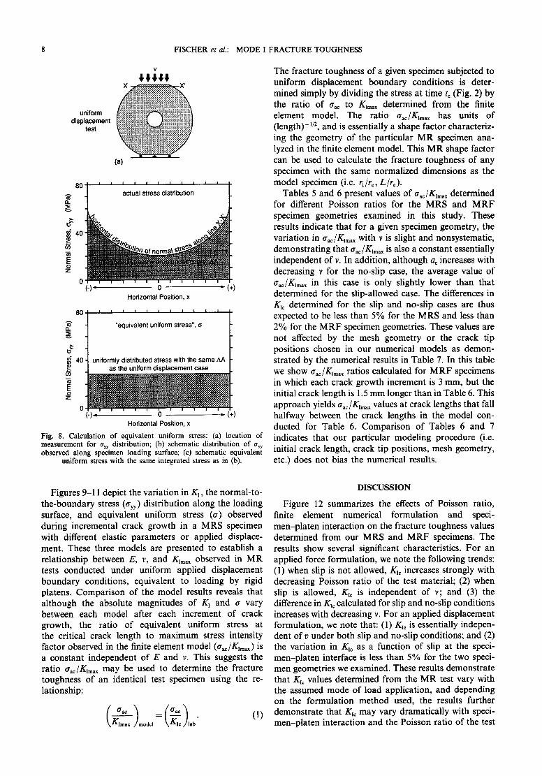
In our displacement formulation of the MR test, a uniform vertical displacement (v) is applied to one loading surface and the other surface is fixed [Fig. 4(b)]. Although any arbitrary values of v, v, and E can be chosen for the model, we chose values representative of granular, freshwater ice Ih because our experiments were conducted to determine K~c of this material (see [23]). After each increment of crack propagation in the model, we calculate KI, the distribution of normal stress (O'yy) along the specimen loading surfaces, and the "equivalent uniform stress" (a) on the specimen loading surfaces. Under a uniform displacement boundary condition, normal-to-the-boundary stress (ayy) along the specimen loading surfaces is non-uniform and exhibits a concave upwards profile like that shown in Fig. 8(b). To relate this non-uniform stress distribution to the time-varying stress (in a reality a force) recorded in the lab, we first integrate the area under the O'yy distribution, and then calculate an equivalent uniform stress, a: a uniform stress with the same integrated stress as the actual tryy

distribution [Fig. 8(c)]. The normal stress a is assumed to represent the time-varying stress recorded in the lab. Fischer [24] demonstrated the validity of this assumption by applying a uniform stress to a model loading surface, calculating the O'yy distribution, and then determining the equivalent uniform stress along the surface. For the specific case tested, his results show that the equivalent uniform stress is within 0.4% of the designated applied stress.

Table 4. Critical crack lengths (ac) and maximum mode I stress intensities (K~m~x) determined for MRF specimens with normalized dimensions ri/re=O.1709 and L/ro = 0.3077 under slip and no-slip boundary conditions and various Poisson ratios. Results obtained for an applied constant stress (a~c) of 1.053 MPa in models where crack growth was in 3 mm increments starting from an initial crack length (a0 of 20 mm


Poisson ratio (v) ac (mm) K,m~ x (kPa. m 1/2) a c (mm) glmax (kPa. m t/2)

0.10 53 133.16 44 109.41 0.15 50 129.04 44 109.41 0.20 50 126.06 44 109.41 0.25 50 122.70 44 109.41 0.30 50 118.84 44 109.41 0.35 47 115.25 44 109.43 0.40 44 112.31 44 109.43

8 FISCHER e t al.: MODE I FRACTURE TOUGHNESS

uniform displacement

test

(a)

8O

# 4o

O z

80

ft.

# 40

0

0

(-)- o - (+) Horizontal Position, x

i I I I I I I I I I I

"equivalent uniform stress", o

uniformly distributed stress with the same AA as the uniform displacement case

(-). o - (+) Horizontal Position, x

Fig. 8. Calculation of equivalent uniform stress: (a) location of measurement for Oyy distribution; (b) schematic distribution of ayy observed along specimen loading surface; (c) schematic equivalent

uniform stress with the same integrated stress as in (b).

The fracture toughness of a given specimen subjected to uniform displacement boundary conditions is determined simply by dividing the stress at time tc (Fig. 2) by the ratio of aac to Klm~x determined from the finite element model. The ratio O'ae/glmax has units of (length)- t/2, and is essentially a shape factor characteriz- ing the geometry of the particular MR specimen ana- lyzed in the finite element model. This MR shape factor can be used to calculate the fracture toughness of any specimen with the same normalized dimensions as the model specimen (i.e. ri/r e, L/re).

Tables 5 and 6 present values of trJK~m,x determined for different Poisson ratios for the MRS and MRF specimen geometries examined in this study. These results indicate that for a given specimen geometry, the variation in trac/Klmax with v is slight and nonsystematic, demonstrating that o,c/K~m,x is also a constant essentially independent of v. In addition, although ac increases with decreasing v for the no-slip case, the average value of trac/glmax in this case is only slightly lower than that determined for the slip-allowed case. The differences in Kic determined for the slip and no-slip cases are thus expected to be less than 5% for the MRS and less than 2% for the MRF specimen geometries. These values are not affected by the mesh geometry or the crack tip positions chosen in our numerical models as demonstrated by the numerical results in Table 7. In this table we show O'ac/Klmax ratios calculated for MRF specimens in which each crack growth increment is 3 mm, but the initial crack length is 1.5 mm longer than in Table 6. This approach yields aao/Klm~x values at crack lengths that fall halfway between the crack lengths in the model conducted for Table 6. Comparison of Tables 6 and 7 indicates that our particular modeling procedure (i.e. initial crack length, crack tip positions, mesh geometry, etc.) does not bias the numerical results.

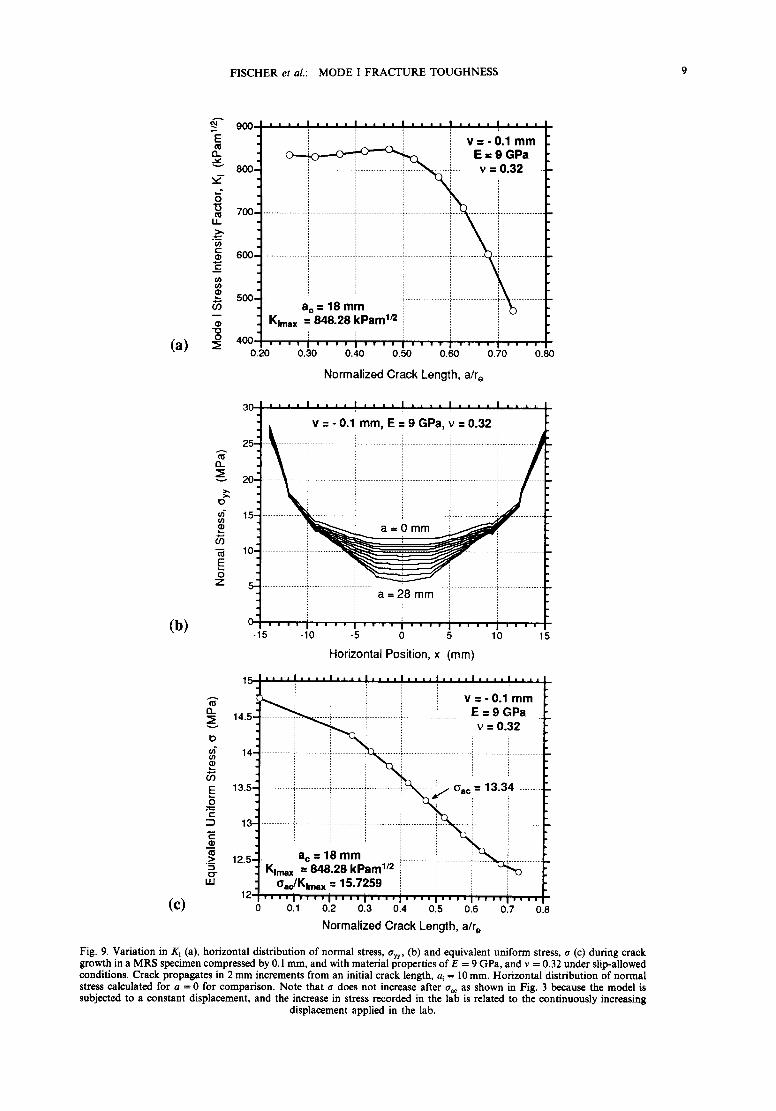
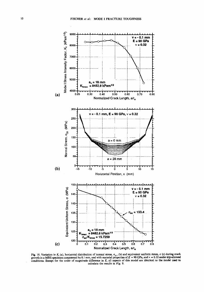
Figures 9-11 depict the variation in K~, the normal-to- the-boundary stress (O'yy) distribution along the loading surface, and equivalent uniform stress (a) observed during incremental crack growth in a MRS specimen with different elastic parameters or applied displacement. These three models are presented to establish a relationship between E, v, and glmax observed in MR tests conducted under uniform applied displacement boundary conditions, equivalent to loading by rigid platens. Comparison of the model results reveals that although the absolute magnitudes of K~ and tr vary between each model after each increment of crack growth, the ratio of equivalent uniform stress at the critical crack length to maximum stress intensity factor observed in the finite element model (O'ac/glmax) is a constant independent of E and v. This suggests the ratio trac/glmax may be used to determine the fracture toughness of an identical test specimen using the relationship:

Klmax /model \KIc/lab"

DISCUSSION

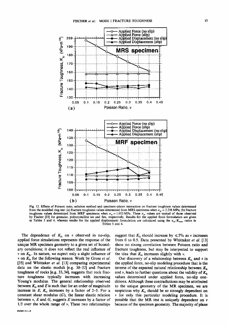
Figure 12 summarizes the effects of Poisson ratio, finite element numerical formulation and specimen-platen interaction on the fracture toughness values determined from our MRS and MRF specimens. The results show several significant characteristics. For an applied force formulation, we note the following trends: (1) when slip is not allowed, Kit increases strongly with decreasing Poisson ratio of the test material; (2) when slip is allowed, K~¢ is independent of v; and (3) the difference in K~ calculated for slip and no-slip conditions increases with decreasing v. For an applied displacement formulation, we note that: (1) K~c is essentially independent of v under both slip and no-slip conditions; and (2) the variation in Kit as a function of slip at the specimen-platen interface is less than 5% for the two specimen geometries we examined. These results demonstrate that K~¢ values determined from the MR test vary with the assumed mode of load application, and depending on the formulation method used, the results further demonstrate that Kx¢ may vary dramatically with specimen-platen interaction and the Poisson ratio of the test

FISCHER e t al.: MODE I FRACTURE TOUGHNESS 9

A

900 . . . . . . . . . . . . . . . . ~ . . . . z . . . .

ii V = - 0 . 1 m m

~. ~ + ,= = 9,+p, + 6oo ......... 2 ~E

+ ++ oo . . . . iiiii iiiiii i!iii iiiii i!ii iiiii iiii iiiiiill i i i ii i! i ilil i i iii ° I • 500 . . . . . . . . . . .

Klm. x =, 848 .28 k P a m 1/2

( a ) ~ 400 . . . . i . . . . i . . . . . . . . i . . . . . . . . | 0.20 0.30 0.40 0.50 0.60 0.70 0.80

N o r m a l i z e d C r a c k Length , a l r o

30 . . . . I . . . . I . . . . I ,, ,, I ,, ,, I ,, ,,

, v = - 0.1 mm, E = 9 GPa, v = 0 .32

+ i iii i i i i l + iii !i ~ 20 . . . . . .

D ~" 15.

+ ii N --~ 10.

o Z 5 . . . . . . . . . . . . . . . . . . . . . . . . . . . . . . . . . . . . . . . . . . . . . . . . . . . .

a = 28 m m

( b ) o . . . . . . . . . . . . i . . . . . . . . . . . .

-15 -10 -5 0 10 15

Hor izon ta l Posi t ion, x (mm)

16 ' ~ :,, . . . . . . . . ': . . . . . . . . . . . . ! . . . . ! . . . .

~.. i i v : - 0 . 1 m m

~-" 14 5 ~ - - ~ - ! ~ " ' ~ ' .... i , E : g G P a " ;I ~ i-- .......... i . . . . . . . . ~i ....... v : 0 . 3 2

IO

E 13.5 a¢ : 13 .34 ........

O

1 3 - i . . . . . . . . i . . . . . . . . . . . . i . . . . . . . . . . . . . i . . . . . . . . i . . . . . . . . . ~. . . . . . . . . i . . . . . . . . . .

° +: ............ 'i:i mm ii iiii iil u.I oae/Klmax = 15 .7259

( c ) 1~, . . . . + . . . . + . . . . + . . . . . . . . . . . . i . . . . . . . .

0.1 0.2 0.3 0.4 0.5 0.6 0.7 0.8

N o r m a l i z e d C rack Length , a/r e

Fig. 9. Variation in K t (a), horizontal distribution of normal stress, ayy, (b) and equivalent uniform stress, a (c) during crack growth in a MRS specimen compressed by 0.1 mm, and with material properties of E = 9 GPa, and v = 0.32 under slip-allowed conditions. Crack propagates in 2 mm increments from an initial crack length, a~ = 10 mm. Horizontal distribution of normal stress calculated for a = 0 for comparison. Note that ~ does not increase after % as shown in Fig. 3 because the model is subjected to a constant displacement, and the increase in stress recorded in the lab is related to the continuously increasing

displacement applied in the lab.


900( ' . . . . . . . . . . . . . . . . i . . . . z . . . .

~E i v = - 0 . 1 m m

a. E = 90 G P a

7000 ... . . . . . . . . . . . . . . . . . . . . . . . . . . . . . . . . . . . . . . . . . . . . . . . . . . . . . . . . . . . . . . . . . . . . . . . . . . . . . . . . . . . . . . . . . . . . . . . LL > .

.'t=~ ( / ) ¢ , -

m 6000 .. . . . . . . . . . . . . . . . . ~- ................. ~ ................. i- ................. [. . . . . . . . . . . . . . . [. ................

I

® K | m a x .= 8 4 8 2 . 8 k P a m . I ~ ' 10 O

= 4000 . . . . i . . . . J . . . . i . . . . . . . . i . . . . / ( ' a~ 0.20 0.30 0 .40 0.50 0 .60 0 .70 0 .80

Normalized Crack Length, a/r o

30C . . . . I . . . . I . . . . I .~ a ~ • I . . . ~ i , , • . : T i ; I

L v = - 0.1 m m , E = 90 GPa , v = 0 .32

. 0 ..•••••••i••••••••••••••i••••••••••••••i••••••••••••••••••••••••••••••i•••••••••..ii! iii'.!i 200 . . . . . .

IO . . o

~ 100,

E .

7 50--" •

0 ( b ) -15 -10 -5 0 5 10 15

H o r i z o n t a l P o s i t i o n , x ( m m )

150 . . . . . . . . . . . . . . . . . . . . . . . . = . . . . I . . . . . .

~ " i V = - 0 .1 m m a_ ~ ~ E = 90 G P a

145,4 .... ~ ............ ~, ............. ,, ............ ~, ........

140,

e - -

~ 130,

a -- Smm L.. i . . . . . . . . . . . :..........__ i . . . . . . . . . . . . . "-~ 125, o" K l m a x = 8 4 8 2 . 8 k P a m 1/2 '

uJ ~ a c / K i m , , x = 1 5 . 7 2 5 9

1 2 o . . . . i . . . . i . . . . i . . . . . . . . . . . . . . . . . . . . (C) 0.1 0.2 0.3 0.4 0.5 0.6 0.7 0.8

N o r m a l i z e d C r a c k L e n g t h , a / r e

Fig. 10. Variation in Kj (a), horizontal distribution of normal stress, ~ryy, (b) and equivalent uniform stress, a (c) during crack growth in a MRS specimen compressed by 0.1 ram, and with material properties o fE = 90 GPa, and v = 0.32 under slip-aUowed conditions. Except for the order of magnitude difference in E, all aspects of this model are identical to the model used to

calculate the results in Fig. 9.

FISCHER et a/.: MODE I FRACTURE TOUGHNESS 11

( a )

A

~E

h

$

i . . . . . . . . . . . . . . . . i v::0'.01mm o I .........

70 . . . . . . . . . . . . . . . . . . i . . . . . . . . . . . . . . . . . i . . . . . . . . . . . . . . . . . i . . . . . . . . . . . . . . . . . i . . . . . . . . . . . . . . . i . . . . . . . . . . . . . . .

60 . . . . . . . . . . . . . . . . . . i . . . . . . . . . . . . . . . . . i . . . . . . . . . . . . . . . . . i . . . . . . . . . . . . . . . . . i . . . . . . . . . . . . . . i . . . . . . . . . . . . . . . .

Kimax = 84 .828 kPam 1/ i [E

4o . . . . i . . . . i . . . . i . . . . . . . . i . . . . ~ • 0.20 0.30 0.40 0.50 0.60 0,70 0.80


(b)

2 . 5 "

13. 2 "

D u~ 1.5. ,=

"~ 1.

o Z

0 . 5 . . . . . . . . . . . . . . . . . . . . . . . . . . . . . . . . . . . . ~ . . . . .

a = 2 8 m m

0 • ' ' ' ' • • • | ' ' ' i • ' w =

/

-15 -10 -5 0

. , , , | = . . = , = , , I . . • . I = , • . I • . . .

• v = - 0 . 0 mm, E : 9 G P a , v = O.32

i i iiii!iiiiiiiiiii I iiiii,ii . . . . . . . . . . . . . . . . . . . . . . . . . . . . . . ~[ .......... . . . . . . . . . . . . . . . ' ~ - ~ . ~ ~ ....... i ...............

, , , , | , , ,

5 10 15

Horizontal Position, x (mm)

1.5

0_ 1.45.

D

¢n 1.4.

~ 1.35. 0 e-

E 1.3.

"~ 1.25- O"

w

1.2 (C) 0

~ ~ ! v - - o . o l ~m

• o = 18 m m . ~ ~ - i . . . . . . . . . . . . .

Klmx ='B4.B2B kPam ~ ' o,,JKimax = 15.7259 i

.... i .... i .... i .... i .... i ............ 0.1 0.2 0.3 0.4 0.5 0.6 0.7 0.8


Fig. 11. Variation in K[ (a), horizontal distribution of normal stress, O'yy, ( b ) and equivalent uniform stress, o (c) during crack growth in a MRS specimen compressed by 0.01 ram, and with material properties o fE = 9 GPa, and v = 0.32 under slip-allowed conditions. Except for the order of magnitude difference in v, all aspects of this model are identical to the model used to calculate

the results in Fig. 9.


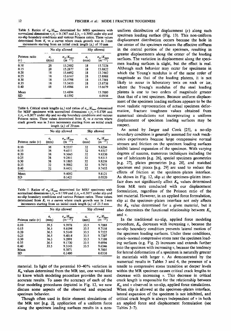
Table 5. Ratios of a~/Kim ~ determined for MRS specimens with normalized dimensions ri/r c = 0.1307 and L / r e = 0.3992 under slip and no-slip boundary conditions and various Poisson ratios. These values determined from K~ vs a curves where crack growth was in 2 mm

increments starting from an initial crack length (ai) of 10 mm


Poisson ratio ao O'ac/Klmax a c aac/Klmax (v) (mm) (m-l/2) (mm) (m-I/2)

0.10 20 15.2482 18 15.7228 0.15 20 15.2877 18 15.8822 0.20 18 15.6492 18 15.7402 0.25 18 15.6167 18 15.8988 0.30 18 15.5798 18 15.7301 0.35 18 15.5453 18 15.8738 0.40 18 15.4986 18 15.6679

Mean 15.4894 15.7880 SD 0.1592 0.0938

Table 6. Critical crack lengths (ac) and ratios of aao/Kt~ ~ determined for MRF specimens with normalized dimensions r~/re = 0.1709 and L/re = 0.3077 under slip and no-slip boundary conditions and various Poisson ratios. These values determined from K l vs a curves where crack growth was in 3 mm increments starting from an initial crack

length (al) of 20mm


ac O'ac/glmax a c O'ac/glmax Poisson ratio (v) (mm) (m -1/2) (mm) (m -l/:)

0.10 38 9.5337 32 9.8204 0.15 38 9.4511 32 9.8317 0.20 38 9.3665 32 9.8330 0.25 38 9.2811 32 9.8313 0.30 38 9.1885 32 9.8258 0.35 32 9.5982 32 9.7972 0.40 32 9.4451 32 9.7453

Mean 9.4092 9.8121 SD 0.1421 0.0320

Table 7. Ratios of aaclKxm~ determined for MRF specimens with normalized dimensions ri/r e = 0.1709 and L / r e = 0.3077 under slip and no-slip boundary conditions and various Poisson ratios. These values determined from K l vs a curves where crack growth was in 3 mm

increments starting from an initial crack length (ai) of 21.5 mm


ao ~ / K t m , x ao a,c/g~m~x Poisson ratio (v) (ram) (m- 1/2) (ram) (m- 1/2 )

0.10 39.5 9.3978 33.5 9.7088 0.15 36.5 9.6194 33.5 9.7158 0.20 36.5 9.5149 33.5 9.7222 0.25 36.5 9.4014 33.5 9.7207 0.30 36.5 9.2891 33.5 9.7108 0.35 36.5 9.1730 33.5 9.6894 0.40 33.5 9.3143 33.5 9.6346 Mean 9.3871 9.7003 SD 0.1480 0.0310

material. In light of the potential 10-40% variation in K~c values determined from the M R test, one would like to know which modeling procedure provides the most accurate results. To asses the accuracy of each of the four modeling procedures depicted in Fig. 12, we now discuss some aspects of the observed and expected specimen behavior.

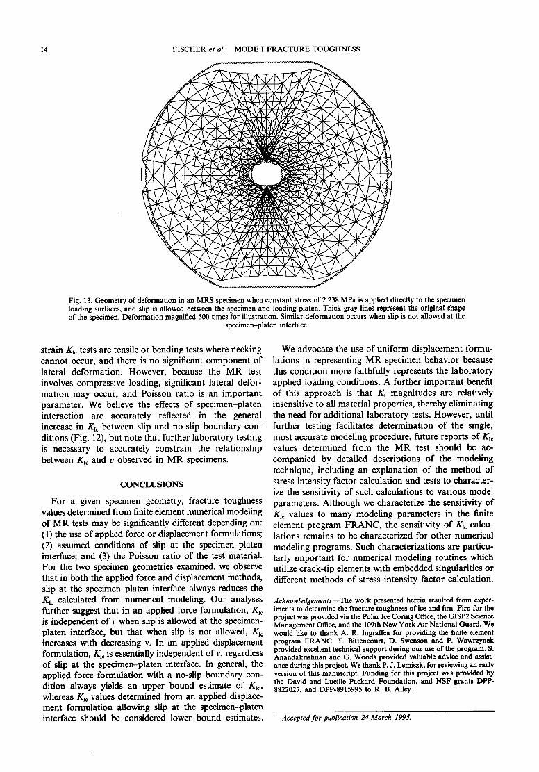
Though often used in finite element simulations of the M R test [e.g. 2], application of a uniform force along the specimen loading surfaces results in a non-

uniform distribution of displacement (v) along each specimen loading surface (Fig. 13). This non-uniform displacement distribution occurs because the hole in the center of the specimen reduces the effective stiffness in the central portion of the specimen, resulting in greater displacements along the center of the loading surfaces. The variation in displacement along the specimen loading surfaces is slight, but the effect is real. Although such behavior may occur for specimens in which the Young's modulus is of the same order of magnitude as that of the loading platens, it is not likely to occur in laboratory tests on rock or ice, where the Young's modulus of the steel loading platens is one to two orders of magnitude greater than that of a test specimen. Because uniform displacement of the specimen loading surfaces appears to be the most realistic representation of actual specimen deformation, fracture toughness values obtained from numerical simulations not incorporating a uniform displacement of specimen loading surfaces may be suspect.

As noted by Jaeger and Cook [25], a no-slip boundary condition is generally assumed for rock mechanics experiments because large compressive normal stresses and friction on the specimen loading surfaces inhibit lateral expansion of the specimen. With varying degrees of success, numerous techniques including the use of lubricants [e.g. 26], special specimen geometries [e.g. 27], platen geometries [e.g. 28], and matched specimen end pieces [e.g. 29] are used to reduce the effects of friction at the specimen-platen interface. As shown in Fig. 12, slip at the specimen-platen interface does not significantly affect K~c values determined from M R tests conducted with our displacement formulation, regardless of the Poisson ratio of the test material. However, in an applied force formulation, slip at the specimen-platen interface not only affects the K~c value determined for a given material, but it also determines the functional relationship between Kic and v.

In the traditional no-slip, applied force modeling procedure, Kit decreases with increasing v, because the no-slip boundary condition prevents lateral motion of the specimen loading surfaces. Under these conditions, crack-normal compressive stress near the specimen loading surfaces (e.g. Fig. 2) increases and extends further into the specimen with increasing v, because the tendency for lateral deformation of a specimen is naturally greater in materials with larger v. As demonstrated by the numerical results in Tables 3 and 4, the presence of a tensile to compressive stress transition at deeper levels within the M R specimen causes critical crack lengths to decrease with increasing v. This decrease in critical crack length is responsible for the relationship between K~o and v observed in no-slip, applied force simulations. When slip is allowed at the specimen-platen interface, lateral expansion of the specimen is not inhibited, and critical crack length is always independent of v in both an applied force and displacement formulation (see Tables 3-7).


E

v

v

f f l

¢-

o

u_

200

1 9 0

180- .

1 7 0 -

1 6 0 -

150-

140

130

0.05

(a)

I -"<>--- Applied Force (no slip) I

. . . . ~ . I . . [ . . ? . . T A~P~P~ ]ied~ DiF°rpP~llaa~lie~)~ Isnlip~lip t

I 0.1 0.15 0.2 0.25 0.3 0.35 0.4 0.45

Poisson Ratio, v

I -----<>-- Applied Force (no slip) I

, . ~ Applied Force (slip) [ 140 ~ . . . . . . . . ': ' ' ' ¢ Applied Displacement (no slip)]

E _1 i ......... . • . Applied Displa~ment (slip) / 135 ............. : .............

130 ............. i . . . . . . . . . . . . . . . . . . . . . . . . . . . . . . . . . . M R F s p e c , m e n u m

125

~ 120 e--

115 o 1-

110 ............ ' .................... .' 2. £ i t , ; , - -

............. i ............. i ............. i ............. i ............. i ............. i . . . . . . . . . . . . . . . . . . . . . . . . . .

100 . . . . j . . . . , . . . . , . . . . , . . . . , . . . . = . . . . . . . .

0.05 0.1 0.15 0.2 0.25 0.3 0.35 0.4 0.45

( b ) Poisson Ratio, v

Fig. 12. Effects of Poisson ratio, solution method and specimen-platen interaction on fracture toughness values determined from the modified ring test: (a) fracture toughness values determined from MRS specimens when tr~ = 2.238 MPa; (b) fracture toughness values determined from MRF specimens when trac= 1.053 MPa. These trac values are typical of those observed by Fischer [23] for granular, polycrystalline ice and tim, respectively. Results for the applied force formulation are given in Tables 3 and 4, whereas results for the applied displacement formulation are calculated using the cr~/K=,,~ ratios in

Tables 5 and 6.

The dependence of K~¢ on v observed in no-slip, applied force simulations represents the response of the unique MR specimen geometry to a given set of boundary conditions; it does not reflect the real influence of v on K~¢. In nature, we expect only a slight influence of v on Kx¢ for the following reason. Work by Gross et al. [35] and Whittaker et al. [13] comparing experimental data on the elastic moduli [e.g. 30-32] and fracture toughness of rocks [e.g. 33, 34], suggests that rock fracture toughness typically increases with increasing Young's modulus. The general relationship observed between K=c and E is such that for an order of magnitude increase in E, K~¢ increases by a factor of 2-5. For a constant shear modulus (G), the linear elastic relation between v, E and G, suggests E increases by a factor of 1/3 over the whole range of v. These two relationships

R M M S 3 3 / I - - B

suggest that K=c should increase by ~< 5% as v increases from 0 to 0.5. Data presented by Whittaker et al. [13] show no strong correlation between Poisson ratio and fracture toughness, but may be interpreted to support the idea that K=c increases slightly with v.

Our discovery of a relationship between Ktc and v in the applied force, no-slip modeling procedure that is the inverse of the expected natural relationship between K== and v, leads to further questions about the validity of Kl¢ values determined under applied force, no-slip conditions. Although these contradictions may be attributed to the unique geometry of the MR specimen, we are suspicious why K~¢ should be so strongly dependent on v for only this particular modeling procedure. It is possible that the MR test is uniquely dependent on v because of the specimen geometry. The majority of plane

14 FISCHER et aL: MODE I FRACTURE TOUGHNESS

Fig. 13. Geometry of deformation in an MRS specimen when constant stress of 2.238 MPa is applied directly to the specimen loading surfaces, and slip is allowed between the specimen and loading platen. Thick gray lines represent the original shape of the specimen. Deformation magnified 500 times for illustration. Similar deformation occurs when slip is not allowed at the

specimen-platen interface.

strain KI~ tests are tensile or bending tests where necking cannot occur, and there is no significant component of lateral deformation. However, because the MR test involves compressive loading, significant lateral deformation may occur, and Poisson ratio is an important parameter. We believe the effects of specimen-platen interaction are accurately reflected in the general increase in K~ between slip and no-slip boundary conditions (Fig. 12), but note that further laboratory testing is necessary to accurately constrain the relationship between K~ and v observed in MR specimens.

CONCLUSIONS

For a given specimen geometry, fracture toughness values determined from finite element numerical modeling of MR tests may be significantly different depending on: (1) the use of applied force or displacement formulations; (2) assumed conditions of slip at the specimen-platen interface; and (3) the Poisson ratio of the test material. For the two specimen geometries examined, we observe that in both the applied force and displacement methods, slip at the specimen-platen interface always reduces the Kic calculated from numerical modeling. Our analyses further suggest that in an applied force formulation, Kic is independent of v when slip is allowed at the specimen- platen interface, but that when slip is not allowed, K~o increases with decreasing v. In an applied displacement formulation, K~c is essentially independent of v, regardless of slip at the specimen-platen interface. In general, the applied force formulation with a no-slip boundary condition always yields an upper bound estimate of K~, whereas K~¢ values determined from an applied displacement formulation allowing slip at the specimen-platen interface should be considered lower bound estimates.

We advocate the use of uniform displacement formulations in representing MR specimen behavior because this condition more faithfully represents the laboratory applied loading conditions. A further important benefit of this approach is that K~ magnitudes are relatively insensitive to all material properties, thereby eliminating the need for additional laboratory tests. However, until further testing facilitates determination of the single, most accurate modeling procedure, future reports of K~0 values determined from the MR test should be accompanied by detailed descriptions of the modeling technique, including an explanation of the method of stress intensity factor calculation and tests to characterize the sensitivity of such calculations to various model parameters. Although we characterize the sensitivity of Kit values to many modeling parameters in the finite element program FRANC, the sensitivity of K~c calculations remains to be characterized for other numerical modeling programs. Such characterizations are particularly important for numerical modeling routines which utilize crack-tip elements with embedded singularities or different methods of stress intensity factor calculation.

Acknowledgements--The work presented herein resulted from experiments to determine the fracture toughness of ice and tim. Firn for the project was provided via the Polar Ice Coring Office, the GISP2 Science Management Office, and the 109th New York Air National Guard. We would like to thank A. R. Ingraffea for providing the finite element program FRANC. T. Bittencourt, D. Swenson and P. Wawrzynek provided excellent technical support during our use of the program. S. Anandakrishnan and G. Woods provided valuable advice and assist- ance during this project. We thank P. J. Lemiszki for reviewing an early version of this manuscript. Funding for this project was provided by the David and Lucille Packard Foundation, and NSF grants DPP- 8822027, and DPP-8915995 to R. B. Alley.

Accepted for publication 24 March 1995.


REFERENCES

1. Thiercehn M. and Roegiers J.-C. Toughness determination with the modified ring test. In Rock Mechanics: Key to Energy Pro- duction. (Edited by Hartman H.L.), pp. 616~22. Proc. 27th U.S. Symp. Rock Mech.: Soc. Mining Engrs, Inc., Littleton, Colo. (1987).

2. Thiercelin M. Fracture toughness under confining pressure using the modified ring test. In Rock Mechanics: Proceedings of the 28th U.S. Symposium on Rock Mechanics. (Edited by Farmer I. W., Daemen J. J. K., Desai C. S., Glass C. E. and Neuman S. P.), pp. 149-156. Balkema, Rotterdam (1987).

3. Thiercelin M., Roegiers J.-C., Boone T. J. and Ingraffea A. R. An investigation of the material parameters that govern the behavior of fractures approaching rock interfaces. In Proceedings of the 6th International Congress on Rock Mechanics. (Edited by Herget G. and Vongpaisal S.), p. 263-269 (1987).

4. Thiercelin M. Fracture toughness and hydraulic fracturing. Int. J. Rock Mech. Min. Sci. & Geomech. Abstr. 26, 177-183 (1989).

5. Srawley J. E. and Brown W. F. Fracture toughness testing methods. In Fracture Toughness Testing and Its Applications. American Society of Testing and Materials Special Technical Publication 381, pp. 133-145 (1965).

6. Kanninen M. F. An augmented double cantilever beam mode of studying crack propagation and arrest. Int. J. Fract. 9, 83-92 (1973).

7. Barker L. M. A simplified method for measuring plane-strain fracture toughness. Engng Fract. Mech. 9, 361-369 (1977).

8. Wawrzynek P. A. and Ingraffea A. R. Interactive finite element analysis of fracture processes: an integrated approach. Theoretical AppL Fract. Mech. 8, 137 150 (1987).

9. Brock D. Elementary Engineering Fracture Mechanics. Sijthoff and Noordhoff, The Netherlands (1986).

10. Lawn B. Fracture o f Brittle Solids, 2nd edn. Cambridge Univ. Press, England (1993).

11. Henshall R. D. and Shaw K. G. Crack tip finite elements are unnecessary. Int. J. Num. Meth. Engng 9, 495-507 (1975).

12. Barsoum R. S. On the use of isoparametric finite elements in linear fracture mechanics. Int. J. Num. Meth. Engng 10, 25 37 (1976).

13. Whittaker B. N., Singh R. N. and Sun G. Rock Fracture Mech- anics: Principles, Design and Applications. Elsevier, Amsterdam (1992).

14. Byskov E. The calculations of stress intensity factors using the finite element method with crack elements. Int. Y. Frac. Mech. 6, 159-167 (1970).

15. Benzley S. E. Representation of singularities with isoparametric finite elements. Int. J. Num. Meth. Engng 8, 537-545 (1974).

16. Li Y. The finite element method by employing the singular elements with concordant displacement at the crack tip. Engng. Fract. Mech. 19, 959-972 (1984).

17. Zienkiewicz O. C. The Finite Element Method in Engineering Science. McGraw-Hill, London (1971).

18. Linsbauer H. N., Ingraffea A. R., Rossmanith H. P. and

Wawrzynek P. A. Simulation of cracking in large arch dam: Part II. J. Struct. Engng 115, 1616-1630 (1989).

19. Ingraffea A. R. Case studies of simulation of fracture in concrete dams. Engng Fract. Mech. 35, 553-564 (1990).

20. Bittencourt T. N., Barry A. and Ingraffea A. R. Comparison of mixed-mode stress intensity factors obtained through displacement correlation, J-integral formulation, and modified crack-closure integral. In Fracture Mech.: 22nd Symp.: Am. Soc. Testing Mater. Spec. Tech. Publn 2, 69-82 (1992).

21. Rybicki E. F. and Kanninen M. F. A finite element calculation of stress intensity factors by a modified crack closure integral. Engng Fract. Mech. 9, 931-938 (1977).

22. Rice J. R. Mathematical analysis in the mechanics of fracture. In Fracture: an Advanced Treatise 2, 227-241 (1968).

23. Fischer M. P., Alley R. B. and Engelder T. Fracture toughness of ice and firn determined from the modified ring test. J. Glaciol. In press.

24. Fischer M. P. Application of linear elastic fracture mechanics to some problems of fracture propagation in rock and ice: Ph.D. thesis, The Pennsylvania State Univ., Univ. Park, PA (1994).

25. Jaeger J. C. and Cook N. G. W. Fundamentals of Rock Mechanics, 3rd edn. Chapman & Hall, London (1979).

26. Engelder T., Logan J. M. and Handin J. The sliding characteristics of sandstone on quartz fault-gouge. Pure Appl. Geophys. 113, 69-86 (1975).

27. Brace W. F. Brittle fracture of rocks. In State of Stress in the Earth's Crust (Edited by Judd W. R.), pp. 111-174. New York, Elsevier (1964).

28. Schulson E. M., Gies M. C., Lasonde G. J. and Nixon W. A. The effect of the specimen-platen interface on internal cracking and brittle fracture of ice under compression: high-speed photography. J. Glaciol. 35, 378-382 (1989).

29. Cook N. G. W. A study of failure in the rock surrounding underground excavations. Ph.D. thesis, Univ. of Witwatersrand (1962).

30. Blair B. E. Physical properties of mine rock, Part 3: U.S. Bureau of Mines Report of Investigations 5130, Washington, D.C. (1955).

31. Blair B. E. Physical properties of mine rock, Part 4: U.S. Bureau of Mines Report of Investigations 5244, Washington, D.C. (1956).

32. Hatheway A. W. and Kiersch G. A. Engineering properties of rock. In Handbook of Physical Properties of Rock (Edited by Carmichael R. S.), Vol. 1, CRC Press, F1 (1982).

33. Senseny P. E. and Pfeifle T. W. Fracture toughness of sandstones and shales. In Rock Mechanics in Productivity and Protection. Proc. 25th U.S. Symp. Rock Mech.: Soc. Min. Engrs Am. Inst. Min., Metall. Petrol. Engrs, Inc., New York, pp. 390-397 (1984).

34. Atkinson B. K. and Meredith P. G. Experimental fracture mechanics data for rocks and minerals. In Fracture Mechanics of Rock (Edited by Atkinson B. K.), pp. 477-525. Academic Press, London (1987).

35. Gross M. R., Fischer M. P., Engelder T. and Greenfield R. J. Factors controlling joint spacing in interbedded sedimentary rocks: integrating numerical models with field observations. J. Geol. Soc. Lond. In press.

Finite Element Analysis of the Modified Ring Test for ...jte2/references/link115.pdf ·...

Documents

Transcript of Finite Element Analysis of the Modified Ring Test for ...jte2/references/link115.pdf ·...