University of Rhode Island University of Rhode Island

DigitalCommons@URI DigitalCommons@URI

Open Access Master's Theses

2015

FINITE ELEMENT ANALYSIS OF A HYDRAULIC SNUBBER WITH FINITE ELEMENT ANALYSIS OF A HYDRAULIC SNUBBER WITH

RESPECT TO HISTORICAL TEST DATA AND AMERICAN SOCIETY RESPECT TO HISTORICAL TEST DATA AND AMERICAN SOCIETY

OF MECHANICAL ENGINEERS REQUIREMENTS OF MECHANICAL ENGINEERS REQUIREMENTS

Matt Palmer University of Rhode Island, mattpalms@yahoo.com

Follow this and additional works at: https://digitalcommons.uri.edu/theses

Recommended Citation Recommended Citation Palmer, Matt, "FINITE ELEMENT ANALYSIS OF A HYDRAULIC SNUBBER WITH RESPECT TO HISTORICAL TEST DATA AND AMERICAN SOCIETY OF MECHANICAL ENGINEERS REQUIREMENTS" (2015). Open Access Master's Theses. Paper 471. https://digitalcommons.uri.edu/theses/471

This Thesis is brought to you for free and open access by DigitalCommons@URI. It has been accepted for inclusion in Open Access Master's Theses by an authorized administrator of DigitalCommons@URI. For more information, please contact digitalcommons@etal.uri.edu.

FINITE ELEMENT ANALYSIS OF A HYDRAULIC

SNUBBER WITH RESPECT TO HISTORICAL TEST

DATA AND AMERICAN SOCIETY OF MECHANICAL

ENGINEERS REQUIREMENTS

BY

MATT PALMER

A THESIS SUBMITTED IN PARTIAL FULFILLMENT OF THE

REQUIREMENTS FOR THE DEGREE OF

MASTERS OF SCIENCE

IN

MECHANICAL ENGINEERING AND SOLID MECHANICS

UNIVERSITY OF RHODE ISLAND

2015

MASTER OF SCIENCE IN MECHANICAL ENGIENERING

OF

MATT PALMER

APPROVED:

Thesis Committee:

Major Professor David Taggart Bahram Nassersharif Fred Vetter

Nasser H. Zawia DEAN OF THE GRADUATE SCHOOL

UNIVERSITY OF RHODE ISLAND 2015

ABSTRACT

Hydraulic snubbers are either acceleration or velocity limiting seismic restraints

designed to restrict movement of piping or equipment during dynamic events or

operational transients. In a piping analysis, snubbers are modeled as linear elastic

spring elements governed by Hooke’s law, F = kx. Snubbers are widely used in

nuclear power plants, and as such their qualification testing to verify the spring

constant k is governed by American Society of Mechanical Engineers (ASME) codes.

ASME mandates experimental determination of spring constant k where practical, or a

combination of testing and analysis when not practical. This qualification test includes

testing at full load under a sinusoidal forcing function at a maximum frequency of 33

Hz.

There remains a practical upper limit to dynamic testing that is imposed by the

availability of test equipment. This upper limit is governed by the size of the hydraulic

pumps and servo actuators supplying fluid to the actuating test cylinder. At current

writing, this limit is approximately 200 kips @ 33 Hz. New reactor designs have

applications for snubbers with load capacities up to 1,900 kips. Functional testing can

be conducted on these large units to verify the lockup and bleed parameters are

correct, as well as the load carrying capacity. However, the dynamic spring rate of the

snubber will not be experimentally verified at full rated load.

This study developed an FEA model of a hydraulic snubber that was compared

to existing ASME qualification test data performed by Anvil Engineered Pipe

Supports (EPS). If an accurate model can be developed for smaller snubber sizes, it

can be used to determine the spring rate of units that exceed the capacity of existing

test equipment.

The experimental test data shows a spring constant that decreases at an

approximately linear rate between 3 Hz and 33 Hz, with a reduction at higher

frequencies of approximately 30%. The simulation models linear elastic behavior, and

shows up to a 6% reduction between 3 Hz and 33 Hz. Part of the discrepancy can be

explained by the load controlled nature of the test negating inertial effects, and

increased deflections due to lost motion caused by assembly clearances and

manufacturing tolerances. Further testing should be conducted, measuring load

through pressure transducers in the cylinder fill ports to overcome these test setup

limitations. This testing should be done on at reduced load so that a model can be

developed that agrees with both the reduced load testing and rated/emergency load

testing.

iv

ACKNOWLEDGMENTS

I would like to acknowledge Professor David Taggart of URI for his assistance in

writing this thesis, and being flexible in working with me.

I would also like to acknowledge Rick Richards of ITT Grinnell Corp and Anvil

Engineered Pipe Supports, as this thesis builds on his 35 years of contributions to the

nuclear power industry.

And to my wife, without whose support this paper would not be possible.

v

TABLE OF CONTENTS

ABSTRACT .................................................................................................................. ii 

ACKNOWLEDGMENTS .......................................................................................... iv 

TABLE OF CONTENTS ............................................................................................. v 

LIST OF TABLES ...................................................................................................... vi 

LIST OF FIGURES ................................................................................................... vii 

CHAPTER 1 ................................................................................................................. 1 

Definition and Principles of Operation of Hydraulic Snubbers………………….1

CHAPTER 2 ............................................................................................................... 12 

History of Dynamic Qualification Testing and Development of ASME

QME/QDR .......................................................................................................... 12

CHAPTER 3 ............................................................................................................... 19 

Dynamic Qualification Testing Conducted By Anvil EPS on Fig. 3306 Hyraulic

Snubbers .............................................................................................................. 19

CHAPTER 4 ............................................................................................................... 39 

FEA Simulation of Dynamic Qualification Testing............................................ 39

CHAPTER 5 ............................................................................................................... 56 

Static and Dynamic Simulation Results .............................................................. 56

CHAPTER 6 ............................................................................................................... 72 

Conclusion and Recommendations ..................................................................... 72

BIBLIOGRAPHY ...................................................................................................... 76 

vi

LIST OF TABLES

TABLE PAGE

Table 1. Spring Rate Values as Reported by Anvil EPS. ........................................... 32

Table 2. Size 35 Spring Rate @ 70° F ....................................................................... 35

Table 3. Size 35 Spring Rate @ 200° F ...................................................................... 35

Table 4. Size 100 Spring Rate @ 70° F ...................................................................... 36

Table 5. Size 100 Spring Rate @ 200° F .................................................................... 36

Table 6. Static Spring Rates As Determined By Simulation ...................................... 56

Table 7. Static Spring Rate With Retaining Ring Gaps .............................................. 58

Table 8. Size 35 Simulation Dynamic Spring Rates ................................................... 59

Table 9. Size 100 Simulation Dynamic Spring Rates ................................................. 59

Table 10. Snubber Dynamic Spring Rate @ 3 Hz ...................................................... 60

Table 11. Size 35 Dimensionless Spring Rates ........................................................... 61

Table 12. Size 100 Dimensionless Spring Rates ......................................................... 62

Table 13. Dimensionless Load .................................................................................... 64

Table 14. Dimensionless Spring Rate with Linearly Increasing Initial Load ............ 69

Table 15. Dimensionless Spring Rate with Linearly Increasing Initial Load Up to .4

Initial Load Utilizing the Acoustic Medium Material Model .................................... 71

vii

LIST OF FIGURES

FIGURE PAGE

Figure 1. Typical Pipe Support Assemblies at Sidi Krir Combined Cycle Power Plant,

Alexandria, Egypt ......................................................................................................... 2

Figure 2. Typical Snubber Assembly. ........................................................................... 2

Figure 3. Snubber Installation at Diablo Canyon Nuclear Power Plant ........................ 3

Figure 4. Grinnell Style Control Valve ......................................................................... 5

Figure 5. Typical Pre-Service Examination Performed at Seabrook Nuclear Power

Station .......................................................................................................................... 7

Figure 6. Typical Oscilloscope Dynamic Test Plots. .................................................... 9

Figure 7. Large bore hydraulic snubber (LBHS) in assembled in a functional test

bench ........................................................................................................................... 14

Figure 8. Size 35 Fig. 3306 ......................................................................................... 19

Figure 9. Size 35/100 Cut-Away Rendering ............................................................... 20

Figure 10. – Size 35 and 100 Fig. 3306 in dynamic test fixtures at National Technical

Systems Labs. .............................................................................................................. 25

Figure 11. Size 100 Prior to High Temperature Drag/Functional Testing .................. 26

Figure 12. Size 100 Fig. 3306 in the Test Setup ......................................................... 26

Figure 13. Size 35 Inside the Makeshift “Oven” During a High-Temperature

Functional Test ........................................................................................................... 27

Figure 14. Zoomed In View of 10 Hz Test ................................................................ 30

Figure 15. NTS Plot of an Entire Test @ 10 Hz ......................................................... 30

viii

Figure 16. Same 10 Hz w/ Load and Deflection Plotted Against Time ...................... 31

Figure 17. Cylinder Drift @ 1 Hz for the Size 35. ...................................................... 34

Figure 18. Snubber Spring Rate By Frequency, Sizes 35 and 100 from Anvil Tests 37

Figure 19. Cylinder ..................................................................................................... 45

Figure 20. Cylinder Head ............................................................................................ 45

Figure 21. Cylinder Endcap ........................................................................................ 45

Figure 22. Pivot Mount ............................................................................................... 45

Figure 23. Piston and Piston Rod Assembly ............................................................... 45

Figure 24. Size 35 Assembly ...................................................................................... 46

Figure 25. Applied Pressure Load of Static Model ..................................................... 50

Figure 26. Cylinder Endcap Mesh .............................................................................. 50

Figure 27. Cavity Tie Constraint ................................................................................. 53

Figure 28. Fixed Cylinder Edge .................................................................................. 53

Figure 29. Dynamic Model Assembly and Mesh........................................................ 54

Figure 30. Location of Concentric Seal Seats ............................................................. 57

Figure 31. Retaining Ring Grooves ............................................................................ 57

Figure 32. Size 35 Dimensionless Spring Rate ........................................................... 61

Figure 33. Size 100 Dimensionless Spring Rate ......................................................... 62

Figure 34. Dimensionless Load Vs Frequency ........................................................... 64

Figure 35. Modified Waveform to Simulate Lost Motion .......................................... 66

Figure 36. Modified Waveform to Simulate Lost Motion and Impact Loading ......... 67

ix

Figure 37. Dimensionless Spring Rate w/ Simulated Deadband ................................ 69

Figure 38. Dimensionless Spring Rate w/ Simulated Deadband Utilizing the Acoustic

Medium Material Model ............................................................................................. 71

1

CHAPTER 1

Definition and Principles of Operation of Hydraulic Snubbers

A pipe support is an integral part of any nuclear power plant. Pipe supports are

load bearing components that support the weight and guide the thermal growth of

safety and non-safety related piping systems and equipment. Pipe supports consist of

nearly infinite configurations, but all have the same recipe:

1) Structural Attachment – Typically consists of a bracket or lug welded to the

building structural steel or bolted to the building foundation or containment

structure

2) Pipe/Equipment attachment – A clamp designed to fit around a pipe or lug

welded to equipment (pump, steam lines, pressurizer, etc)

3) The “middle” – The pipe support component that functions as required by

analysis. Will allow thermal growth, apply a load to the system, or restrain

pipe movement as needed.

Figure 1 shows typical pipe support assemblies on 34” hot reheat lines

at a natural gas combined cycle power plant. When in operation, these lines

will operate at a temperature of approximately 1050° F, causing several inches

of thermal movement. Figure 2 is a typical snubber assembly per Figure NF-

1132-1(c) [1]. There are many other types of pipe support components, but for

the purposes of this paper, the discussion will be limited to shock and sway

suppressors, also known as snubbers.

2

Figure 2 – Typical Snubber Assembly [1]

Figure 1 - Typical Pipe Support Assemblies at Sidi Krir Combined Cycle plant Alexandria, Egypt. Note the

snubber in the background orthogonal to the run pipe. Palmer, Matt 2010

3

A snubber is a type of seismic restraint whose design was first conceived in the

1960’s and began to see large scale use in the nuclear power industry in the 1970’s [2,

3]. In a typical installation, it is attached to the building structure by a rear bracket and

the piping system or equipment by a clamp, as in Figure 2. When the piping or

equipment heats up during normal operation, a snubber is designed to allow thermal

growth while applying minimal or no load to the system. It is operating in a passive

mode. When subject to a velocity or acceleration greater than the pre-set limit, the

restraint activates and applies resistance to any motion. Figure 3 shows a snubber

installed on main steam piping at Diablo Canyon Nuclear Power Plant

Figure 3 – Snubber installation at Diablo Canyon Nuclear Power Plant. Kewalramani, Mohan “Support 414-414BSL”.

2010

4

These passive and active modes of operation are common to the two types of

snubbers present in industry today: Mechanical and hydraulic. Mechanical snubbers

restrain motion through a ratcheting mechanism or an inertial mass limited to a pre-set

angular acceleration. Hydraulic snubbers utilize valves to restrict the flow of fluid

between the tension and compression sides of a hydraulic cylinder. Both mechanical

and hydraulic snubbers can be velocity or acceleration limiting. This study is limited

to velocity limiting hydraulic snubbers, specifically those manufactured by the Anvil

Engineered Pipe Supports located in North Kingstown, RI (Formerly known as

Grinnell Corp.).

Principles of Operation of Hydraulic Snubbers

Hydraulic snubbers are very similar in operation to any hydraulic actuator

found commonly in industrial equipment, such as a forklift, hydraulic press, excavator

etc… The primary difference is in the valve configuration. Where hydraulic actuators

create motion of a piston rod by pumping fluid into either the tension or compression

side of the cylinder, hydraulic snubbers resist motion by restricting fluid flow out of

the tension or compression side. This fluid resistance through the valves prevents free

movement of the piston, and a load is applied to the piping or equipment in the

opposite direction of system motion. All snubbers are double acting, and will provide

a resisting force in either tension or compression.

5

Functional Characteristics

Functional characteristics are so called because they can be field tested to

verify that the snubber will perform its function as a dynamic restraint. The valve is a

crucial component for the operability of a hydraulic snubber. On Anvil hydraulic

snubbers, it consists of a check and bleed valve set in parallel on both the tension and

compression sides. The check or lockup valve, is of the spring loaded poppet type. The

bleed valve is a flow restrictor which provides resistance to flow as function of

pressure. A typical control valve arrangement is shown in Figure 4.

Figure 4 – Grinnell style control valve. [4]

In passive mode, the check valve is held open with a spring, and as fluid starts

to flow over the poppet, a pressure differential develops between the reservoir and

6

cylinder side. As fluid flow velocity increases, the pressure difference becomes large

enough to overcome the force of the spring holding the valve open. At this point, the

snubber goes from passive to active, and the poppet closes. Fluid must now flow

through the flow restrictor. Enough resistance is provided that the pressure inside the

cylinder begins to increase, and a load is applied through the piston and piston rod.

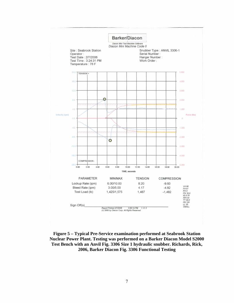
A typical snubber pre-service test plot is shown in Figure 5. The test plot

shows the two functional characteristics of a snubber that must be within specification

to be installed in a nuclear power plant. These characteristics are defined in [5] as

follows:

Activation – The change of condition from passive to active, in which the

snubber resists rapid displacement of the attached pipe or component

Release Rate – The rate of the axial snubber movement under a specified load

after activation of the snubber takes place

In the passive region, piston velocity is increased gradually. There is a minimal

force required to move the snubber. This is referred to as drag. When the snubber

piston velocity reaches the pre-set activation velocity, the fluid flow rate through the

control valve is sufficient to close the poppet valve. In the test plot, this occurs at a

piston rod velocity 8.2 inches per minute (IPM) in tension, and 9.6 IPM in

compression. After activation, the load applied to the snubber piston rod is increased

up to the load specified in the release rate, and the piston velocity is plotted as a

function of load. In this case, the snubber has a release rate of 4.17 IPM in tension and

4.82 IPM in compression at a load of approximately 1500 lbf.

7

Figure 5 – Typical Pre-Service examination performed at Seabrook Station Nuclear Power Plant. Testing was performed on a Barker Diacon Model S2000 Test Bench with an Anvil Fig. 3306 Size 1 hydraulic snubber. Richards, Rick,

2006, Barker Diacon Fig. 3306 Functional Testing

8

A fundamental understanding of the functional characteristics of snubbers is

required for interpretation of the dynamic test and simulation results discussed later.

However, the activation velocity and release rate values have minimal effect on the

dynamic performance of a hydraulic snubber. In the 1970’s there was a large study

done by the Grinnell Corporation on the effect of varying lockup and bleed velocities

on dynamic spring rate [6]. It was determined that an upper limit of 40 IPM activation

velocity and 25 IPM release rate would have negligible effect on the dynamic

performance and operability of a snubber. Further discussion on the mechanisms of

lockup and bleed are not relevant.

Drag force is defined in [5] as “The force that will sustain low-velocity

snubber movement without activation throughout the working range of the snubber

stroke”. It is not of interest in most functional tests of hydraulic snubbers. Typical

values for hydraulic snubbers are 2% or less of rated load. A snubber with a rated load

of 10 kips should see a drag force of no more than 200 lbf. This resistance to motion is

primarily caused by friction between the energized elastomeric seals and

cylinder/piston rod. In most piping analysis, this drag force is neglected.

Dynamic Characteristics

Plant operations and maintenance personnel are concerned with the functional

characteristics of a snubber; Plant design engineers are more concerned about the

dynamic characteristics. These engineers analyze piping systems and equipment for

their response to a ground excitation or operational transient, including water hammer,

turbine trip, or pipe rupture. In their models, snubbers are placed at key node points to

9

restrain motion of the system and reduce piping stresses to within American Society of

Mechanical Engineers (ASME) code allowables. To simplify analysis, an assumption

is made that the seismic or transient velocities of piping and equipment are much

greater than the pre-set activation velocity of a snubber. It can then be assumed that

the snubber is a linear elastic spring element subject to Hooke’s law, F = kx.

When subjected to a sinusoidal load, hydraulic snubbers exhibit a

load/displacement relationship that follows a hysteresis loop, as shown in Figure 6.

Figure 6 – Typical oscilloscope dynamic test plots [8]

From the plot in Fig. 6, the numerical value of k, or the dynamic spring rate of a

snubber can be derived. The vertical axis represents load, and the horizontal axis

displacement. The load and displacement of each cycle are plotted against one

another, and the peak to peak loads and displacements are measured. Spring rate is

defined in [9] as the “Applied load in tension and compression divided by the recorded

10

displacements in tension and compression”. This corresponds to the equation

. The result k is usually given in units of kips/in.

The region of non-linear motion is known as “dead band”. This is free-motion

of the hydraulic snubber while activated with no resistance being applied to the piping

or equipment. This is a consequence of clearances required for installation of load pins

in the rod eye and pivot mount or mechanical gaps in the assembly due to

manufacturing tolerances. At low frequencies ( < 3 Hz), it is also includes the time

required for the snubber poppet valve to close as the snubber cycles between tension

and compression.

In practice, there are real limitations to the usefulness of the spring rate

parameter of a hydraulic snubber. The two primary factors that contribute to a

snubber’s spring rate are the bulk modulus of the fluid and the position of the piston in

the cylinder. Fluid bulk modulus can vary from batch to batch, as well as with

temperature and pressure. For traditional hydraulic snubbers of a single piston rod

configuration, the difference in fluid volumes of the tension and compression sides

creates a different response for each position of piston travel. One can imagine the

difficulties of accurately predicting the ambient temperature at each snubber location,

as well as accurately modeling thermal movements to predict snubber piston position.

The number of analysis load cases would grow exponentially.

To circumvent this complexity, the nuclear power industry wrote plant design

specifications to include a Minimum Spring Rate parameter. In first generation design

of large scale commercial reactors, overly conservative assumptions of accident

conditions led to very stiff piping systems [12]. This then required manufacturers to

11

supply snubbers that will always be at least as stiff as the minimum spring rate value.

This made analysis of large piping systems practical. For very critical equipment

applications, such as steam generator, pressurizer, or reactor coolant pump snubbers,

the engineer may specify a spring rate and require that the manufacturer test each

production unit to verify the dynamic performance is within spec. This presents its

own set of challenges and is the motivation for this study.

12

CHAPTER 2

History of Dynamic Qualification Testing and Development of ASME QME/QDR

Early snubber populations in the 1970’s and early 1980’s were prone to failure

on a very large scale. Depending on the number of snubbers in service at each plant,

failure rates hovered between 4% - 30% [2]. Fluid and seal compatibility issues with

radiation and temperature caused many snubbers to leak or clog the valves, impairing

their safety related function. Minimal or non-existent codes and requirements for

snubber design qualification testing resulted in a low degree of confidence of their

operability during a seismic event or transient. Compounding the problem is the fact

that many early plant designs had upwards of 1000+ snubbers on their piping systems

[2]. Optimizing seismic support locations in a piping analysis is an iterative process,

and during the design phase of many plants, it was cheaper to buy more snubbers than

it was to run hundreds of analysis iterations on mainframe computers. In some cases,

entire plant populations were tested and/or replaced each refueling cycle at great

expense in radiation exposure to plant workers, time and money.

The NRC began to address the issue of snubber operability as early as 1978,

and incorporated it into its standard review of all licensee safety analysis by 1980 [11].

This put the onus on the licensee to provide proper assurance that safety related

hydraulic snubbers would be operable during postulated seismic events or transients.

Another consequence of the high failure rate of early snubbers was the development of

13

GE Specification 21A3502. This purchasing specification [13] addressed many

deficiencies of hydraulic snubber design identified in the late 1960’s and early 1970’s,

including environmental conditions, materials of construction, and dynamic

performance. Many elements of this document made it into the Grinnell Corporation’s

design specification for hydraulic snubbers. By 1992, approximately 57% of all

hydraulic snubbers installed in nuclear power plants were supplied by Grinnell [4]. As

a result of this industry dominance, many of the design requirements from the GE

specification became the accepted industry standard.

By the early 1980’s, the issue of snubber operability had been solved from a

regulatory standpoint [11]. Licensees began snubber reduction programs, more

rigorous inspection regimens, and adoption of improved hydraulic snubber designs.

However, it was also apparent that most licensees had two distinct snubber

populations that required different approaches to qualification of the design and in-

service inspection. Licensees and snubber vendors differentiated snubbers as large-

bore and small-bore, sometimes also referred to as equipment and piping snubbers.

The common definition of a large bore snubber is a snubber with a rated load of 50

kips or greater, and as of 1992, large bore snubbers made up approximately 10% of the

US hydraulic snubber population [4].

A typical snubber maintenance plan for both large and small bore snubbers

involves:

Visual inspection of a pre-determined sample size

14

Verification through testing of functional parameters of a pre-

determined sample size. Figure 7 shows a typical hydraulic snubber test

bench arrangement

Verification of functional parameters of snubbers that fail visual

inspection

Expanded functional testing scope if a pre-determined number of

functional test failures occur

Repair or replacement of failed snubbers.

In practice, functional testing and snubber repair/replacement activities involve

removal of the snubber from service and installation onto a test bench. This can

present real issues inside the containment structure, as space is limited and any time

spent performing maintenance activities exposes plant personal to radiation. For small

Figure 7 – Large bore hydraulic snubber (LBHS) in assembled in a functional test bench. [4]

15

bore piping snubbers, many designs are light enough that they can be carried by hand

or maneuvered through tight spaces with minimal trouble.

Large bore equipment snubbers are much larger in size. Some cylinders have

piston diameters as large as 20” and can weigh several thousand pounds. In many

cases, it was deemed impractical to do any functional testing and prior to 1980, most

large bore hydraulic snubbers were classified as inaccessible and were not subject to

the same in-service functional testing of piping snubbers [4]. To rectify this, the NRC

issued Generic Letters 80-99 and 84-13 [19, 20] requiring that all licensees add large

bore hydraulic snubbers to their snubber surveillance populations. The first in-service

functional tests of large bore hydraulics occurred at 13 plants between 1982-84. Each

of these 13 plants had large equipment snubbers that failed to activate during testing,

and would have been inoperable during a seismic event. In fact, all 14 steam generator

snubbers at Palisades were found to be inoperable since initial reactor startup [10].

As a result of these serious safety deficiencies, the NRC created Generic Issue

113 which culminated in the technical evaluation NUREG/CR-5416, published in

1992 [4]. The technical evaluation determined that one of the main causes of large

bore snubber failures was the lack of qualification testing for early designs. In many

cases, design requirements for large bore snubbers were not properly specified by the

licensee. Test equipment limitations in the 1960’s and 1970’s also prevented full scale

static or dynamic testing of larger sizes. In fact, some designs did not see a proof-load

test to verify that they were indeed capable of operating at full rated load. However, a

survey of five large bore snubber manufacturers yielded that by 1992, qualification

16

tests that were very similar to the GE 21A3502 requirements had been conducted for

many models with a rated loads of under 100 kips.

One of the recommendations made in NUREG/CR-5416 was to implement a

uniform set of qualification standards for large bore hydraulic snubbers, either through

a regulatory guide issued by the NRC or the addition of snubber qualification

requirements to the existing ASME Qualification of Mechanical Equipment (QME)

standard. ASME created a subgroup of the QME code to develop this standard. Given

that the test requirements of GE 21A3502 had been adopted by several manufactures

and were well understood by much of the industry, this specification became the basis

for the development of the new testing standard. This standard became known as

“Qualification of Active Mechanical Equipment Used in Nuclear Facilities Section

Qualification of Dynamic Restraints”, also known as QME/QDR [9]. QME-1-2007

was the first QME standard to be endorsed by the NRC for rulemaking in 2009 [14].

Current Snubber Qualification Testing

Nuclear power plants designed to ASME Section III 2007 or later must have

their dynamic restraints qualified per ASME QME/QDR. The minimum requirements

for functional and dynamic testing are outlined in in QME/QDR-6223.1 and presented

in abbreviated form here

QDR-6223.1(a): Activation velocity or acceleration, as applicable, in both

tension and compression

QDR-6223.1(b): Release rate in tension and compression at 5%, 10%, 25%,

50%, 100% of rated load and at a specified emergency load

17

QDR-6223.1(c): Initial force required to move the snubber in tension and

compression (break-away drag, analogous to static friction)

QDR-6223.1(d): Drag force throughout the entire range of travel in tension and

compression

QDR-6223.1(e): Measurement of Dead band

QDR-6223.1(g): The spring rate shall be tested by a dynamic cyclic loading

equal to the rated load (or other specified load). The peak displacement range,

including the dead band, shall be obtained during the dynamic cyclic test

through the peak force range. The peak force range shall include load applied

in opposite directions. Restraint movement shall be centered about the ¼, ½,

and ¾ stroke locations according to the requirements of the functional

specification. The testing frequency shall be from 3 Hz to 33 Hz at intervals of

approximately 3 Hz. Each frequency shall last not less than 10 sec. Response at

each frequency shall be recorded as load-displacement traces. No extreme

change in displacement should be observed from one frequency to the next, as

this could indicate that the fundamental frequency (natural frequency) resides

in the 3 Hz - 33 Hz range.

QDR-6223.1(g) is written in its entirety here so the scope of dynamic tests

involved in qualifying a hydraulic snubber is clear to the reader. Where testing is

deemed unreasonable, qualification can be performed through dynamic testing at

lower frequencies, drop testing, parent restraint qualification, analysis, or any

combination thereof. The upper limit of 33 Hz requirement is not arbitrary. Reg.

Guide 1.60 [7], issued in 1973, gives guidance on the design values of ground

18

acceleration up to a frequency of 33 Hz. Frequencies above 33 Hz are assumed to be

outside postulated seismic events.

Motivation for the study

There remains a practical upper limit to dynamic testing that is imposed by the

availability of test equipment. This upper limit is governed by the size of the hydraulic

pumps and servo actuators supplying fluid to the actuating test cylinder. At current

writing, this limit is approximately an input load of 200 kips @ 33 Hz. New reactor

designs, including the Westinghouse AP1000 plants under construction at Vogtle and

VC Summer sites, have applications for snubbers with rated loads up to 1900 kips.

Functional testing can be conducted on these large units to verify the lockup and bleed

parameters are correct, as well as the load carrying capacity. However, the dynamic

spring rate of the snubber will not be experimentally verified at full rated load.

The purpose of this study is to develop an FEA model of a hydraulic snubber

that can be compared to existing data of tests performed by Anvil Engineered Pipe

Supports (EPS). If an accurate model can be developed for smaller snubber sizes, it

could be used to determine the spring rate of units that exceed the capacity of existing

test equipment.

19

CHAPTER 3

Dynamic Qualification Testing Conducted By Anvil EPS on Fig. 3306 Hydraulic

Snubbers

Anvil EPS developed a second generation snubber in the late 1990’s. This

snubber is known as a Figure 3306 (Figure 8). At Anvil EPS, each part is given an

arbitrary numerical designation, or Figure number. This snubber line has 7 sizes of

various strokes, with load ratings from 350 lbf to 120,000 lbf. This study focuses on

the size 35 and size 100 models.

Figure 8 – Size 35 Fig. 3306

20

Common Features:

The Anvil Fig. 3306 sizes 35 and 100 share some common features. They are

both cylindrical in shape and have internal fluid reservoirs. The control valves are

mounted inside the piston. The size 35 and 100 are different from the rest of the line in

that they utilize dual piston rods.

.

Figure 9 – Fig. 3306 Size 35/100 Cut-Away Rendering

The following description assumes a movement that causes the cylinder piston

rod to retract. The rod eye is connected by a pin to the piping or equipment to be

21

restrained. Movement is transmitted to the piston from the rod eye via the front piston

rod. The pivot mount is pinned to a rear bracket, and the piston moves relative to the

cylinder. This is known as the compression side. The piston displaces fluid on the

compression side, and it flows through the control valves into the tension side. The

cylinder and piston dimensions are such that the rod eye can move a magnitude of 6”

from the fully retracted position to the fully extended position. This is referred to as

cylinder stroke. A piston at mid-stroke can retract or extend 3” relative to the fixed

pivot mount.

The rear piston rod is not load bearing but does provide key advantages. It

provides more resistance to side loading by keeping the piston aligned in the cylinder

under large lateral accelerations. It also equalizes the surface area of the piston on the

tension and compression sides, which does two things:

- The primary fluid reservoir can now be sized for thermal

expansion/contraction only and does not need to include volume for fluid

displacement due to piston rod retraction.

- Deflection of an incompressible fluid column has the same load/displacement

relationship as an axially loaded elastic member, or , where β is the fluid

bulk modulus, and P, L, and A are the applied load, fluid column length, and

piston area. For single rod hydraulic cylinders, the equation for peak to peak

deflection due to the fluid columns under sinusoidal loading is

with the subscripts T and C denoting the tension and compression sides. The

lengths of the tension and compression fluid columns add up to the total length

22

of snubber stroke, or . When tension and compression piston areas

are equal, fluid deflection simplifies to

and is now no longer a function of piston position.

Materials of Construction

Many different materials go into the construction of a Fig. 3306. The piston,

piston rods, and endcap are of carbon steel construction, either SA-36 or A-108

Grades 1018CW thru 1050CW. The cylinder tube is either SA-513 or SA-519, Grades

1018CW thru 1026CW . The cylinder head is made of SA-564 Type 630 age hardened

at 1075° F stainless steel. The piston rod and pivot mount are SA-193 Gr. B7 chrome

alloy, and the cap screws are high-strength SA-434 Class BC carbon steel.

The pressure differential developed over the poppet valve is partly a function

of viscosity, thus snubber activation is also viscosity dependent. The viscosity of the

working fluid must be relatively stable through a variety of environmental conditions.

The fluid is a silicone polymer known as polydimethyldiphenylsiloxane, and is widely

used in many brands of hydraulic snubbers. This silicone based fluid was originally

manufactured by General Electric under the brand name GE SF-1154. A critical

characteristic of this fluid is its excellent viscosity stability when exposed to radiation.

It has been tested by Anvil EPS up to 1 10 rads of gamma exposure with no

significant gelation. Its viscosity is also fairly stable at elevated temperatures. This

provides more consistent functional test results, as field testing is not always done in a

temperature controlled setting.

23

For the load/displacement relationship of interest in this study, fluid bulk

modulus is of great importance. As mentioned previously, fluid bulk modulus can vary

from batch to batch. At the time Anvil’s testing was carried out, Anvil was in the

process of qualifying a new fluid vendor, and the lot of fluid used in the qualification

tests underwent laboratory analysis to determine the bulk modulus. This laboratory

testing was done at 70° F and will be used for this study. For simulations at 200° F,

experimental bulk modulus data is not available and historical Anvil data will be used.

Fig. 3306 Qualification Testing to ASME QME/QDR Requirements

The Fig. 3306 is a second generation snubber that was intended to be utilized

by new build plants invoking ASME B&PV Design code Section III 2007 or later. A

full campaign of qualification testing was conducted at four different labs for all seven

sizes, culminating in the 2009 testing of the size 35 and 100. Testing for these sizes

was conducted at National Technical Systems in Santa Clarita, CA. Over the course of

several months, the full suite of QDR qualification tests were conducted as outlined in

Anvil procedure PE 9851-3 [21]. Of particular interest in this study is the test setup in

Figures 10 through 13.

Each snubber was pinned at the pivot mount to a fixed bracket and to an

actuating hydraulic cylinder at the rod eye. A linear transducer was mounted on the

rod eye and cylinder head to measure deflection of the rod eye relative to the cylinder

(Figure 11). This configuration does not measure cylinder deflection, and an

assumption was made that cylinder axial deflection was minor compared to fluid

column deflection. It is worth noting that in this test configuration, in addition to

24

cylinder deflection in tension, the clearance between the pins, spherical bearings, rear

bracket holes, and the pivot mount deflections, are not taken into account.

A load cell was placed in the load path between the actuating cylinder and

snubber rod eye. In addition to measuring the load applied to the snubber, the load cell

provides feedback for actuator load control. Load control is utilized to prevent the

snubber from generating high working pressures inside the cylinder. As the loaded

fluid column deflects, the unloaded column will draw fluid from the secondary

reservoir to prevent cavitation in the unloaded side. Under displacement control, the

additional fluid volume creates a higher pressure and over the course of many cycles,

internal pressure can become high enough to cause seal failure. By using load control,

this can be avoided.

The rated load of each cylinder is applied by the actuating cylinder with a

sinusoidal waveform at frequencies between 1 Hz – 33 Hz. Cylinder load and

displacement were sampled at a time increment of .0002 seconds. During testing, it

was determined that there was electronic “noise” in the system, and 150 Hz filter was

placed on both the load and deflection outputs to filter out high-frequency signals.

Data was recorded into LabView software, and made available in a format readable to

Microsoft Excel.

25

Figure 10 – Size 35 and 100 Fig. 3306 in dynamic test fixtures at National Technical

Systems Labs. Richards, Rick, 2009

26

Figure 11 – Size 100 prior to high temperature drag/functional testing. Note the linear transducer banded to the cylinder and mounted to the rod eye. Heat was pumped into a foam board enclosure around the snubber that was used as an insulating layer to maintain a snubber temperature of 200° F. Richards, Rick,

2009

Figure 12 – Size 100 Fig. 3306 in the test setup. NTS Labs had two machines configured for snubber testing, a smaller unit for drag force and functional testing (foreground, with snubber mounted), and a larger machine for high

frequency dynamic testing (background). The actuating cylinder and load cells are visible for both test setups on the left hand side of the photo. Richards, Rick,

2009

27

Loading and Deflection Direction Conventions

During the tests, a direction convention was established that cylinder extension

is positive, and cylinder retraction is negative. A load applied that causes the cylinder

piston to move outward relative to the body is positive and any load that causes piston

movement inward relative to the cylinder body is negative. Also, extension and

retraction are sometimes referred to as the tension and compression sides. Forces that

place the snubber in tension are positive, and forces that place the snubber in

compression are negative.

Because the size 35 and 100 cylinders feature a double piston rod, all dynamic

testing conducted by Anvil on these sizes took place with the cylinder approximately

at mid-stroke, or 3” from full cylinder retraction. The linear transducer to measure

Figure 13 – Size 35 inside the makeshift “oven” during a high temperature functional test. The size 100 can be seen mounted on the large test machine at the top of the photo. Richards, Rick, 2009

28

displacements was zeroed at mid-stroke. All displacement values are given relative to

this zeroed value. A positive value indicates the piston has extended from mid-stroke;

a negative value indicates the piston has retracted.

Test Sequence and Data Reduction by Anvil EPS (PE 9851-6)

The full test sequence conducted by Anvil EPS includes all functional and

dynamic testing mandated by QME/QDR. After testing was conducted, the data was

reduced by Anvil EPS to come up with numerical values for snubber spring rate. To

reduce the data, the following method was employed:

1) Review the raw lab data files using the proprietary NTS Plot File Viewer. This

program enables the user to view tab delimited text files and plot values on an

X and Y axis. Displacement was plotted on the X axis, and Time on the Y Axis

(Fig. 14)

2) Using NTS Plot Viewer, scale the X and Y axis until the extrema of individual

cycles are visible in the plot (Fig. 15). Record the start and end times of the

cycles that are of interest

3) Open the tab-delimited .dat files in Microsoft Excel.

4) Locate the rows with the cycles of interest in the spreadsheet. Plot load on the

primary axis, displacement on the secondary axis for approximately 5-10

cycles.

5) Draw a line of best fit between the maximums of each cycle. Repeat for the

minimums of each cycle.

29

6) Record the values of maximum and minimum displacement where the lines of

best fit intersect the secondary axis (Fig 16).

7) Determine spring rate of the cylinder according to QDR-4110(g), or

As stated previously, the position of the linear transducer does not record lost

motion or cylinder/pivot mount deflection. To accurately determine spring rate,

these values of deadband and cylinder deflection were calculated and added to the

total deflection. The spring rate values published by Anvil EPS reflect this

additional deflection. To simplify data reduction, the spring rate values reported in

this paper do not reflect lost motion or cylinder/pivot mount deflections. This

includes all experimental data presented in this section and simulation outputs

presented later.

30

Figure 15 – NTS Plot of an entire test @ 10 Hz

Figure 14 – Zoomed in view of 10 Hz test

31

Figure 16 – Same 10 Hz w/ load and deflection plotted against time. Note line of best fit drawn between maximum and minimum and minimum

deflections. [15]

32

Spring Rate Values as Reported by Anvil EPS [15, 16]

Table 1 - Spring Rate Values as Reported by Anvil EPS

   Spring Rate kips/in

Freq (Hz) Size 35

Ambient Size 35 200° F

Size 100 Ambient

Size 100 200° F

1  1,033  822  1,870  1,827 

2  1,248  935  2,102  2,115 

3  1,342  997  2,170  2,178 

5  1,379  996  2,115  2,026 

10  1,346  1,021  2,036  1,915 

15  1,259  1,002  1,900  1,760 

20  1,195  957  1,761  1,666 

25  1,078  1,041  1,758  1,560 

30  1,035  811  1,410  1,578 

33  940  833  1,431  1,569 

Data Reduction Through Use of Computer Code

One of the challenges Anvil faced in reducing the data was the sheer volume of

information. As an example, Figure 16 shows 5 cycles of a test that lasted for 12

seconds at 10 Hz, for a total of 120 cycles. The spring rate value was determined by

using only 4% of the available data. To some degree, the reduction of the test data is

subject to a small bias by selection of different cycles, or to interpretation of the

analyst, or where the line of best fit is drawn on a particular day.

To work with a larger set of data and remove graphical interpretation from the

equation, code was written in Microsoft Excel Visual Basic for Applications, or VBA

to return the extrema for each cycle in the selected time period. The user must still

choose a start and end time of the cycles in question; the recorder was on before a load

was applied to the system, and the actuating cylinder takes several cycles to ramp up

33

to the desired load. This can be seen in Figure 15, where it takes approximately 12

seconds to achieve the minimum test load of 100 kips peak to peak, and the last 5

seconds have no meaningful data. Once the start and end times are specified, the start

and end of each cycle is periodic as a function of the test frequency. By iterating

through each cycle, the maximums and minimums can be extracted for the entire test.

One behavior that is evident in the dynamic test plots is drift of the piston

position over the course of the test. In Fig. 15, the initial piston position is

approximately .22” extended from mid-stroke. At the end of the test, piston position

has experienced some “drift”, and traveled to -.25” retracted from mid-stroke. This

phenomenon is characteristic of all hydraulic snubbers. The mechanism of drift is not

well understood, and is a combination of fluid flow through the check valves and

bleed valves under cyclic loading. If the test is long enough, under load control the

snubber will reach equilibrium when the stiffness in tension equals the stiffness in

compression and the drift will stop.

34

An understanding of the drift mechanism is not required for determining spring

rate. Fig. 17 plots the displacement extrema of 5 cycles at 1 Hz. Upon inspection, it is

apparent that the maximums and minimums of each cycle drift by approximately -

.025” each cycle. This “drift” will skew the peak to peak displacements depending on

how they are measured. Using the 2nd cycle as an example, measuring the distance A

will result in a smaller displacement than measuring peak to peak distance B. Because

snubber “drift” happens at a rate that is approximately linear, the peak to peak

displacements A and B can be averaged to find the true peak to peak distance.

Figure 17 – Cylinder drift @ 1 Hz for the Size 35

35

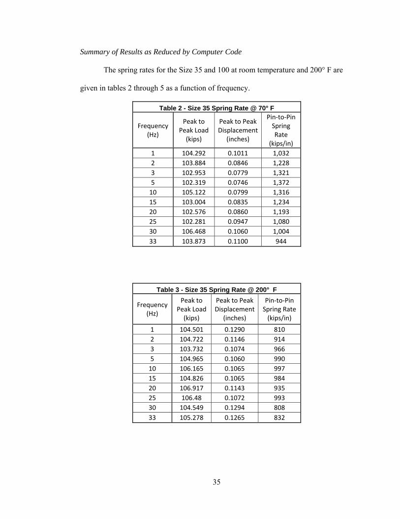
Summary of Results as Reduced by Computer Code

The spring rates for the Size 35 and 100 at room temperature and 200° F are

given in tables 2 through 5 as a function of frequency.

Table 2 - Size 35 Spring Rate @ 70° F

Frequency (Hz) 

Peak to Peak Load (kips) 

Peak to Peak Displacement 

(inches) 

Pin‐to‐Pin Spring Rate 

(kips/in) 

1  104.292  0.1011  1,032 

2  103.884  0.0846  1,228 

3  102.953  0.0779  1,321 

5  102.319  0.0746  1,372 

10  105.122  0.0799  1,316 

15  103.004  0.0835  1,234 

20  102.576  0.0860  1,193 

25  102.281  0.0947  1,080 

30  106.468  0.1060  1,004 

33  103.873  0.1100  944 

Table 3 - Size 35 Spring Rate @ 200° F

Frequency (Hz) 

Peak to Peak Load (kips) 

Peak to Peak Displacement 

(inches) 

Pin‐to‐Pin Spring Rate (kips/in) 

1  104.501  0.1290  810 

2  104.722  0.1146  914 

3  103.732  0.1074  966 

5  104.965  0.1060  990 

10  106.165  0.1065  997 

15  104.826  0.1065  984 

20  106.917  0.1143  935 

25  106.48  0.1072  993 

30  104.549  0.1294  808 

33  105.278  0.1265  832 

36

Table 4 - Size 100 Spring Rate @ 70° F

Frequency (Hz) 

Peak to Peak Load (kips) 

Peak to Peak Displacement 

(inches) 

Pin‐to‐Pin Spring Rate 

(kips/in) 

1  260.254  0.1452  1,792 

2  259.748  0.1257  2,066 

3  257.218  0.1187  2,167 

5  254.338  0.1280  1,987 

10  251.203  0.1318  1,906 

15  255.892  0.1441  1,776 

20  258.132  0.1568  1,646 

25  254.991  0.1632  1,562 

30  252.200  0.1587  1,589 

33  246.551  0.1557  1,584 

Table 5 - Size 100 Spring Rate @ 200° F

Frequency (Hz) 

Peak to Peak Load (kips) 

Peak to Peak Displacement 

(inches) 

Pin‐to‐Pin Spring Rate (kips/in) 

1  261.459  0.1390  1,881 

2  257.558  0.1228  2,097 

3  252.803  0.1181  2,141 

5  253.784  0.1222  2,077 

10  246.334  0.1239  1,988 

15  247.801  0.1306  1,897 

20  253.702  0.1471  1,725 

25  252.289  0.1466  1,721 

30  247.265  0.1720  1,438 

33  248.302  0.1714  1,449 

37

Fig. 18 – Snubber Spring Rate by Frequency, Sizes 35 and 100 from Anvil tests

Interpretation of Test Data

Figure 18 shows two separate sizes, the size 35 and 100, at two different

temperatures, 70° F and 200° F, for a total of four test sequences. Each test sequence

shows the same behavior; Spring rate reaches a maximum value somewhere between

3 Hz and 10 Hz, with declining values as a function of frequency. The Size 35 and 100

high temperature tests have a lower spring rate than the room temperature tests, as

expected. The working fluid, SF-1154, has a bulk modulus that decreases with

temperature.

Looking at Fig. 18 in more detail, each test plot shows a sharp increase in

spring rate from 1 Hz to 3 Hz. At lower frequencies, these valves spend a larger

38

percentage of time in the open position, allowing fluid to flow between the tension and

compression sides. This fluid flow causes larger displacements, reducing snubber

stiffness.

The test data shows a maximum stiffness value at approximately 3 Hz. At

frequencies greater than 3 Hz, fluid flow through the check valves is minimal, and it

can be assumed there is no fluid flow (aside from drift) between the tension and

compression sides. For the size 35, the values of spring rate are relatively constant

between 5 Hz – 15 HZ and appear to be independent of frequency in this region. As

frequency increases to 33 Hz, the values trend down, indicating a softening of the

snubber as frequency increases. For the size 100, this downward trend occurs

immediately after a maximum spring rate at 3 Hz.

39

CHAPTER 4

FEA Simulation of Dynamic Qualification Testing

To develop an analytical model that can be tested against experimental data, an

FEA simulation was created using ABAQUS version 6.13, published by the Simulia

Corporation. The objective of the simulation is to reproduce the spring rate values in

Fig. 18. To this end, both static and dynamic models were developed. The static model

is geometrically accurate and used to determine that the units are consistent, the

applied load does not grossly deform the cylinder, and the deflections are the expected

order of magnitude. The dynamic model is a simple axisymmetric representation of

the snubber used to isolate the fluid behavior.

Assumptions

1) No fluid exchange occurs between the tension and compression sides of the

cylinder

It is assumed that the poppet style check valves are in the closed

positon the entire length of the simulation, and there is no fluid transfer

between the tension and compression sides of the cylinder through the bleed

valves. The test data supports that the opening and closing of these valves only

has an impact for frequencies lower than 3 Hz, and the frequencies of interest

40

here are between 3 Hz – 33 Hz. This assumption was made to reduce the

number of elements and stay away from the realm of CFD simulations.

2) “Walking” does not occur

A consequence of Assumption 1 is that snubber drift does not occur.

The test data shows that this drift adjusts the deflection extrema at a linear rate,

and this has been taken into account in the experimental test data reduction. It

will not have any impact on the cycle to cycle values of deflection in the

simulation.

3) Fluid bulk modulus is not variable w/ pressure

During dynamic cycling, the internal pressure of a snubber will

increase above the value due to the applied load. For example, if the snubber

cycles first in tension, the compression fluid column will deflect, causing fluid

to flow into the tension side from the reservoir. As the snubber moves to a

neutral position, the pressure on the compression and tension sides balances at

a non-zero value. With no bleed valves, this value asymptotically approaches

the pressure that would be present at full load with each cycle. When the

snubber is now in a neutral position of zero deflection, it is pressurized in the

tension and compression sides at 1 X full load. When a load is applied, the

loaded side is at a pressure that is 2 X full load, and the unloaded side is at

zero.

In actuality, some of this pressure is bled off through the bleed valves

at a pressure dependent rate. There is no test data that shows what actual

pressure inside the cylinder is during a dynamic event, and it is assumed that

41

ΔP between the tension and compression sides is 2 X full load. In the

simulation, with Assumption 1, ΔP will still be 2 X full load, although the

loaded side will be pressurized to 1 X rated load and the unloaded side will in a

vacuum at – 1 X rated load.

4) Fluid deflection governs the response to load

In the dynamic model, it is assumed that steel deflections are orders of

magnitude smaller than the deflection of the fluid. This assumption is valid, as

Young’s modulus for steel is approximately 150 X the bulk modulus of the

hydraulic fluid.

Fluid Cavity Material Models

Two material behaviors were developed for the fluid cavity:

1) Fluid Cavity Interaction

This behavior models a fluid cavity as a linear elastic volumetric spring [18],

with properties of density and bulk modulus. A fluid cavity is defined by an

enclosed surface with normal pointing inward. The elements are surface

elements, but they are coupled to a cavity reference node that has properties of

pressure and volume. As the surface elements deform due to an external load

or internal pressure, the pressure and volume properties of the reference node

are updated to the new conditions. These properties are then applied to the next

step or increment. This interaction can be used with both implicit and explicit

static and dynamic procedures.

42

2) Hydrodynamic Equation of State

This material model can be used to simulate both compressible and viscous

behavior. ABAQUS provides several examples utilizing a linear Mie-

Grüneisen equation of state to model discretized fluid deformation [18].

Energy is dissipated either through volumetric or shear deformation. The user

must specify density, viscosity, and the speed of sound through the material,

which is a function of bulk modulus and density.

Output from the fluid cavity interaction and the equation of state model agree

within a few percentage points. The data presented in the output section uses the

cavity interaction for the static model, and equation of state for the dynamic model.

Discretizing the fluid as acoustic elements was also examined with very similar results

to the other two material models.

Choice of Procedures

The general/static procedure was chosen for the static model primarily for ease

of use in creating a complicated model of linear elastic behavior. Several iterations of

the model were developed, beginning with a very simple fluid cavity and cylinder with

an applied load that did not vary with time. The outputs of the simulation could then

be verified by hand. As more complicated elements were added to the model, the

model behaviors could be quickly compared to the test data or an expected result.

For the dynamic model, the explicit/dynamic procedure is used. This procedure

satisfies equations of motion at increment n, and uses the acceleration of that

increment to advance the model to the next n + 1 increment. The explicit dynamics

43

procedure allows for a time history of linear response to be modeled. It has been

verified through testing that the natural frequency of the size 35 and size 100 snubbers

does not exist in the frequencies of interest, therefore all load/deflection response is

expected be linear.

A consequence of using this procedure is the required time increment can be

very small compared to the static simulation and can lead to long run times for the

same model. The minimum time increment is the time required for the dilatation wave

to pass through the smallest element in the model [18]. Complicated geometries that

cause large elements to distort or require small elements for an accurate model can

decrease the time increment by orders of magnitude for the rest of the model, greatly

increasing run times. This drove some differences in the static and dynamic models to

keep run times on the order minutes. It is worth noting that implicit dynamic and

modal based procedures were also tried, with similar results.

Static Model Geometry

The first simplifying assumption in the model is recognizing that the hydraulic

cylinder is round, and the number elements can be reduced by using symmetry. The

pivot mount and rod eye are both rectangular in shape, and because of this ¼

symmetry was used in the XY and YZ planes. The cylinder is oriented so the Y axis is

parallel with the axis of the snubber cylinder. +Y is cylinder extension, and –Y is

cylinder retraction. The Fig. 3306 consists of hundreds of individual parts. In order to

reduce the number of contact interactions and elements, many subassemblies were

merged together to form continuous pieces. This model consists of 6 parts:

44

1) Cylinder – Modeled as a 3D solid. For the Size 35, the cylinder ID is 5”

and the wall thickness is .5”, and with a thickness to ID ratio of .1, a thin-

walled cylinder model could be used. However, the Size 100 has a ratio of

.125, and the assumption of a thin walled cylinder cannot be made. In order

to achieve consistency between the 35 and 100 simulations, they were

modeled as solids. Partitions to the internal diameter surface had to be

made to accurately describe the fluid cavities. There are also bolt holes at

the cylinder ends (Fig. 19).

2) Cylinder Head – Modeled as 3D solid. This part is part of the cavity

surface boundary and includes bolt holes (Fig. 20)

3) Cylinder End Cap – Modeled as a 3D solid. This piece is only modeled so

as to include bolts and the threaded connection of the pivot mount to the

cylinder. Included in the model are the bolt holes (Fig. 21)

4) Pivot Mount – Modeled as 3D solid. This piece is used for the boundary

conditions at the pin hole (Fig. 22).

5) Piston and rod assembly – Modeled as a 3D solid. A partition was made in

the rod eye to apply a load, and in the piston rods to describe the fluid

cavity (Fig. 23)

6) Bolts – Modeled as 2D wire features. These bolts were modeled as wires to

reduce the number of elements in the model. They are partitioned to

include a node for a bolt pre-load force.

45

Figure 19 - Cylinder

Figure 20 - Cylinder Head Figure 21 – Cylinder Endcap

Figure 22 Pivot Mount Figure 23 – Piston and Piston Rod Assembly

46

Figure 24 – Size 35 Assembly

Materials – Static Model

The steel parts were modeled as homogenous, isotropic materials. 4 different

grades of steel were used in the model. Density and Poisson’s ratio are the same for all

four, with Young’s modulus having slightly different values. The material properties

are as follows [17]:

Poisson’s Ratio: .3

Density: 7.35 10 ∙

Low Carbon Steel ( < .3%): 29.2 10

High Carbon Steel ( > .3%): 29.4 10

Low Chrome Alloy: 29.6 10

17-4 Stainless Steel: 28.5 10

A variation in Young’s modulus and density with temperature will have minimal

effect on the model, and was not considered.

47

The silicone hydraulic fluid has properties of density and bulk modulus in the

model. Assumption 3 states that for the purposes of the model, the bulk modulus is not

pressure dependent. The values used in each simulation are determined by the pressure

at rated load. These values are

Bulk Modulus @ 70° F = 1.98 10

Bulk Modulus @ 200° F = 1.46 10

Density @ 70° F = 9.822 10 ∙

Density @ 200° F = 8.949 10 ∙

The units of density are not in as is more commonly seen in literature and

reference books. This is a consequence of the choice of units of the applied load and

geometry. Inches were chosen as the fundamental unit of length for ease of solid

modeling, and units of lbf were chosen as units of force. From , units of mass

are now ∙

and density is ∙

. To convert to the correct units, divide by the

conversion factor

32.17 ∙12

Static Model Interactions and Constraints

For the static model, the master/slave surface contact definition was used for

all interactions of solid parts that come into contact. In this contact definition, pressure

is transmitted between the two surfaces. The slave surface is not allowed to penetrate

the master surface, although both surfaces are allowed to deform. Friction is not

48

expected to have a significant effect in the model, so frictionless behavior was used.

The fluid cavity interaction was used for both the tension and compression cavities.

The cavity reference nodes lie on the axis of the cylinder. There is also a tie constraint

between the pivot mount and the cylinder end cap. This constraint ties the movement

and rotation of the nodes on both surfaces together via the master/slave relationship.

To simulate the bolted connections of the cylinder head and endcap to the

cylinder, multi-point beam constraints were used. This constraint ties the displacement

and rotation of a single control point to the nodes that lie on a slave surface. They are

connected by an idealized rigid beam. The wire bolt features had two multipoint

constraints; One from the bolt “head” to the counter-bored surface, and a second from

the threaded end to the internal threads of the cylinder.

Static Model Boundary Conditions

There are four boundary conditions applied to the model

1) Symmetry in the XY plane

2) Symmetry in the ZY plane

3) Fixed surface at the pivot mount pin

4) Fixed X and Z translation at the rod eye exterior flat plane. This is to prevent

any moment developing around the fixed pivot mount surface. In actuality,

these nodes would be part of a pinned connection and no moment would

develop.

49

Static Model Applied Loads

1) Bolt preload

This load is applied to an internal node of the wire features used for bolts. This

load is applied during the first step after the initial step to determine the deformed

lengths of the bolts under the pre-load. This deformed length is then applied to step

2.

2) Primary Loading of the Cylinder

This load is the applied load to the rod eye and simulates a pin applying a

distributed load over 45° of the rod eye ID (Fig. 25). Due to ¼ symmetry, the

magnitude of the load will be ¼ the experimental test value. Because it is a

pressure distribution acting over 45°, the input magnitude will be greater than the

actual value according to the equation

4∙ cos

/

This amounts to an increase of 1.111 for the simulation input from the actual test

load. The portion of the load not directed down the axis of the snubber will cancel

due to symmetry. There is no input waveform for the static model. It is applied

instantaneously in compression in one step, and in tension in a second step.

Static Model Mesh

ABAQUS has a mesh generation algorithm that has a parameter known as seed

size. The algorithm places nodes on the model edges, and these nodes are the seed

nodes. Seed size refers to the spacing between these nodes, and when possible, node

spacing maintains this value throughout the model. ABAQUS suggests a default seed

50

size based on part geometry and element type. Contact models work best with

elements of similar size, so the smallest default seed size was used for the entire

model. This is governed by the cylinder head and endcap, which have a default seed

size of .42 for the size 35 model, and .71 for the size 100. General purpose continuum

elements were utilized. Due to the complex geometries, quadratic tetrahedral C3D10

elements were selected. Various seed sizes were tried, both larger and smaller, and the

default provided results that were good enough at a reasonable computational cost.

(Fig. 26). For the bolts, B31beam elements with a seed size of .062 and .069 were

used.

Figure 25 – Applied Pressure Load of Static Model

Figure 26 – Cylinder Endcap Mesh

51

Dynamic Model Geometry

To isolate the fluid behavior, a very simple axisymmetric model was created.

Because of Assumption 4, the rod eye and cylinder portion between the compression

cavity and the pivot mount could be neglected. This model consisted of three parts, all

modeled as planar shells:

1) Cylinder

Models the cylinder and head as one piece. The interior edge was partitioned to

specify cavity surfaces.

2) Piston and Rod Assembly

Models the piston and piston rods as one piece. To more accurately model the

mass of the part, the interior portion of the rear piston rod was removed for the

secondary reservoir cavity.

3) Fluid

Discretized rectangle.

Dynamic Model Materials

For simplicity, only one steel material was modeled. It has the following

properties:

Poisson’s Ratio: .3

Density: 7.35 10 ∙

@ 70° F: 29.0 10

@ 200° F: 28.0 10

52

Variations in Young’s modulus with temperature were applied in this model,

as it will change the speed of wave propagation through the steel parts. Density varies

less than 1% with from 70° F to 200° F, and this was neglected.

The fluid is modeled using the equation of state material model. It has the

following properties:

Wave Speed @ 70° F: 44773

Wave Speed @ 200° F: 39706

Viscosity @ 70° F: 9.827 10 ∙

Viscosity @ 200° F: 3.6 10 ∙

Density @ 70° F: 9.822 10 ∙

Density @ 200° F: 8.949 10 ∙

Dynamic Model Interactions, Constraints, Boundary Conditions, Loadings

The dynamic model contained no interactions. To enforce continuity between

the fluid and steel, a tie constraint between the nodes on the edge of the discretized

fluid cavities and the steel cavity surface was created. (Figure 27) The fluid edges

were the slave surface. This constraint models the no-slip condition of Newtonian

fluids, where the fluid nodes on the interface of the steel-fluid boundary share

displacement of the steel.

The only boundary condition needed to prevent rigid body motion is a fixed

cylinder base where it would extend to the pivot mount. (Figure 28). The load is

applied as a pressure on the main piston rod. It has a sinusoidal amplitude of the form

53

∙ sin

This load was applied for .5 seconds for 3 Hz to 5 Hz and .25 seconds for frequencies

between 10 Hz and 33 Hz.

Dynamic Model Mesh

The dynamic model is more sensitive to changes in mesh density. The fluid is a

much softer material than the steel, and must be a much finer mesh. For the size 35,

the piston rod had a seed size of .5, the cylinder .25, and the fluid .15. The size 100

had elements of .75, .5, and .3 respectively. The steel and fluid of both models used

axisymmetric solid CAX4R elements.

Figure 27 – Cavity Tie Constraint Figure 28 – Fixed Cylinder Edge

54

Figure 29 – Dynamic Model Assembly and Mesh

Output

The output of the static and dynamic models includes the deflection of the

piston rod and the reaction forces from the fixed axial constraint. These constrained

nodes lie on the pivot mount in the static model, and on the cylinder in the dynamic

model. In the static model, loading takes place over two steps of time increment 1. In

the dynamic model, values were written to the output database at time increments of

.0004 seconds for 3 Hz and 5 Hz and .0002 seconds for 10 Hz – 33 Hz. The deflection

of the piston rod relative to the fixed cylinder was measured from the motion of a

single node on the axis of symmetry.

In the Fig. 3306 qualification testing, there was not much variation cycle to

cycle of the input load. This is a consequence of the load controlled nature of the test.

55

Therefore, to determine spring rate, the maximum magnitude of the input load can be

doubled to obtain the peak to peak load. This is divided by the peak to peak deflection.

The reaction forces of the nodes fixed in the axial direction relative to the snubber can

be summed. The difference in the summed reaction forces and the input load show the

inertia effects of the piston/piston rod mass moving with high accelerations.

56

CHAPTER 5

Static and Dynamic Simulation Results

Static Results

The static spring rates from the ABAQUS models are shown in Table 6

Table 6 ‐ Static Spring Rate As Determined by Simulation 

   Temperature Input Load 

(kips) 

Peak to Peak Deflection (inches) 

Static Spring Rate (kips/in) 

% Deviation 3 Hz Experimental 

Size 35 70° F  52.210  0.0683  1,529  16% 

200° F  52.210  0.0874  1,195  24% 

Size 100 70° F  127.465  0.0676  3,771  74% 

200° F  127.465  0.0859  2,968  39% 

It was assumed in the experimental data that at 3 Hz, the activation valves were

closed and had no effect on piston deflection. The spring rate at 3 Hz is as close to

static as the experimental data can get. When measured against the static model, it

appears that the values are not in agreement. However, this discrepancy can be

explained by the configuration of the reservoir and compression cavity.

The low pressure primary fluid reservoir is sealed off from the high pressure

compression fluid cavity with elastomeric seals seated in concentric plates (Figure 30).

These concentric plates are held in place by internal retaining rings (Figure 31). On the

size 35, these retaining rings are .109 ± .003 inches thick, and the retaining ring

groove is .123 ± .002 inches wide. With no tolerances taken into account, with one

ring there would be a gap of .014”. The gap caused by two retaining rings plus the

tolerance stackups of the concentric seal seats creates uncertainty in the length of the

57

fluid reservoir. When the cylinder cycles in tension, the compression cavity goes to

zero pressure, and the primary reservoir spring pushes the seal seats towards the

tension cavity. As soon as the pressure in the compression side climbs above the

reservoir pressure, the seal seats move towards the pivot mount, which causes the

entire cavity to drift and adds lost motion to the cycle. On the size 100, the gap of one

ring is .026”

Figure 30 – Location of Concentric Seal Seats

Figure 31 – Retaining Ring Grooves

58

In the ABAQUS model, the seal gland disks were modeled rigidly connected to

the cylinder, and not floating between two retaining rings. When two gaps are added

to the peak to peak static deflection, the resulting static spring rate is shown in Table 7

Table 7 ‐ Static Spring Rate with Retaining Ring Gaps 

   Temperature Input Load 

(kips) 

Peak to Peak Deflection (inches) 

Static Spring Rate (kips/in) 

% Deviation 3 Hz Experimental 

Size 35 70° F  52.210  0.0963  1,084  ‐18% 

200° F  52.210  0.1154  905  ‐6% 

Size 100 70° F  127.465  0.1196  2,132  ‐2% 

200° F  127.465  0.1379  1,849  ‐14% 

These values are in much closer agreement with the experimental data. The

values of % Deviation at 3 Hz are negative because with the retaining ring gaps, the

simulated stiffness is less than the experimental data. Without measuring the actual

thickness and widths of the retaining rings, retaining ring grooves, and seal seat disk

thickness, the amount of lost motion cannot be known. To determine the minimum

static spring rate through simulation, the maximum gap width and minimum

thicknesses should be summed and included as lost motion. This lends further validity

to Assumption 4, that the deformation of the metal parts under load is minor compared

to the fluid behavior and now also the manufacturing tolerances and installation

clearances in the seal seat assembly and pinned connections.

59

Dynamic Simulation Results

The dynamic simulation results utilizing the equation of state material model

and a dynamic explicit procedure are as follows in Tables 8and 9

Table 8 ‐ Size 35 Dynamic Spring Rate 

Peak to Peak Input Load of 104.065 kips 

   70° F  200° F 

Frequency Peak to Peak Deflection (inches) 

Spring Rate (kips/in) 

Peak to Peak 

Deflection (inches) 

Spring Rate (kips/in) 

3  0.0776  1,341  0.1003  1,038 

5  0.0777  1,339  0.1006  1,034 

10  0.0783  1,329  0.1014  1,026 

15  0.0788  1,321  0.1022  1,018 

20  0.0795  1,309  0.1032  1,008 

25  0.0801  1,299  0.1040  1,001 

30  0.0805  1,293  0.1049  992 

33  0.0809  1,286  0.1053  988 

Table 9 ‐ Size 100 Dynamic Spring Rate 

Peak to Peak Input Load of 252.081 kips 

   70° F  200° F 

Frequency Peak to Peak Deflection (inches) 

Spring Rate (kips/in) 

Peak to Peak Deflection (inches) 

Spring Rate 

(kips/in) 

3  0.0702  3,591  0.0898  2,807 

5  0.0702  3,591  0.0903  2,792 

10  0.0709  3,555  0.0911  2,767 

15  0.0714  3,531  0.0917  2,749 

20  0.0719  3,506  0.0922  2,734 

25  0.0726  3,472  0.0932  2,705 

30  0.0730  3,453  0.0942  2,676 

33  0.0731  3,448  0.0949  2,656 

Mechanical gaps were not included in the peak to peak deflections.

Assumption 4 states that deformation of the steel cylinder is minor compared to the

larger fluid deflections, and can be ignored. This means that variations in geometry

60

between the axisymmetric dynamic model and the experimental test data can be

ignored as long as the fluid behavior is modeled accurately. Using 3 Hz as the

frequency where spring rate is near static, Table 10 shows that the values for “static”

spring rate are the correct order of magnitude and the axisymmetric model is realistic.

Arbitrarily adding mechanical gaps or altering geometries of the steel components will

not make the dynamic results any more or less valid.

Table 10 ‐ Snubber Dynamic Spring Rate @ 3 Hz 

Snubber Size 

Temperature (°F) 

Simulation Spring Rate (kips/in) 

Experimental Spring Rate (kips/in) 

% Difference 

35 70  1,341  1,321  2% 

200  1,038  966  7% 

100 70  3,591  2,167  66% 

200  2,807  2,141  31% 

To compare the effect of frequency on spring rate between the experimental

data and simulation outputs, dimensionless spring rates can be calculated, with 3 Hz

equal to 1. The data is presented in tabular form for the Size 35 and Size 100 in tables

11 and 12, and graphically in Figures 32 and 33

61

Table 11 ‐ Size 35 Dimensionless Spring Rates 

   Simulated  Experimental 

Frequency  70° F  200° F  70° F  200° F 

3  1.0000  1.0000  1.0000  1.0000 

5  0.9987  0.9966  1.0383  1.0251 

10  0.9911  0.9887  0.9966  1.0319 

15  0.9848  0.9810  0.9338  1.0187 

20  0.9761  0.9715  0.9029  0.9683 

25  0.9688  0.9640  0.8176  1.0282 

30  0.9640  0.9557  0.7603  0.8364 

33  0.9592  0.9521  0.7148  0.8615 

Figure 32 – Size 35 Dimensionless Spring Rate

62

Table 12 ‐ Size 100 Dimensionless Spring Rates 

   Simulated  Experimental 

Frequency  70° F  200° F  70° F  200° F 

3  1.0000  1.0000  1.0000  1.0000 

5  1.0000  0.9945  0.9169  0.9700 

10  0.9901  0.9858  0.8795  0.9286 

15  0.9832  0.9793  0.8195  0.8862 

20  0.9763  0.9740  0.7597  0.8056 

25  0.9669  0.9636  0.7210  0.8038 

30  0.9616  0.9533  0.7333  0.6715 

33  0.9603  0.9463  0.7307  0.6766 

Figure 33 - Size 100 Dimensionless Spring Rate

63

Discussion of Dynamic Test Results

The frequency dependence of spring rate in the experimental data is much

greater than the simulation. Experimentally, the difference in spring rate between 3 Hz

and 33 Hz is approximately 30%, and in the simulation is less than 6%. The 6%

deviation in the simulation is due to the inertia of the piston and piston rod assembly.

This inertia can be seen by measuring the reaction forces of the fixed nodes at the

cylinder wall. When the reaction forces in the direction of the applied load are

summed, the value is larger than the maximum value of the sinusoidal input.

Inertia should be seen in the experimental data. Under load control, the applied

force ramps up at a higher rate for each cycle, causing larger accelerations of the

actuator ram and thus larger inertial forces. The simulation data confirms this;

Maximum accelerations at 3 Hz for the size 35 room temperature simulation is 250 ,

and 2870 at 33 Hz. However, the experimental data shows no discernable increase

in input load as a function of frequency. Table 13 shows dimensionless load as

calculated from the reaction forces of the fixed nodes in the simulation, and as

measured from the load cell in the experimental data. Figure 34 shows this

graphically. There is a linear increase in reaction forces in the simulation, but no

pattern in the experimental data.

64

Table ‐ 13 Dimensionless Load 

   Size 35 @ 70° F  Size 100 @ 70° F 

Frequency  Simulated  Experimental  Simulated  Experimental 

3  1.0000  1.0000  1.0000  1.0000 

5  1.0018  0.9938  1.0009  0.9888 

10  1.0102  1.0211  1.0118  0.9766 

15  1.0196  1.0005  1.0206  0.9948 

20  1.0294  0.9963  1.0288  1.0036 

25  1.0350  0.9935  1.0411  0.9913 

30  1.0427  1.0341  1.0468  0.9805 

33  1.0487  1.0089  1.0487  0.9585 

Figure 34 – Dimensionless Load Vs. Frequency

65

The reaction forces in the simulation are measured at nodes that are fixed

relative to the moving piston assembly, and the load cell in the qualification tests was

mounted on a moving actuator ram. Under load control, feedback from the load cell

would cause the actuator to try to compensate for any inertial effects by increasing or

decreasing load to the pre-determined test value. Actual values of load applied to the

snubber are probably greater than the experimental test values. This would increase

the stiffness of the experimental values and reduce their frequency dependence.

The two fluid parameters modeled include bulk modulus and shear viscosity of

the hydraulic fluid. Experimentally, the bulk modulus of SF-1154 increases with

pressure. Working pressures inside the hydraulic snubbers are higher than the

simulated values, both due to the effect of the secondary reservoir adding fluid to the

unloaded side each cycle, and increased loads cause by inertia. At higher frequencies,

the pressure will be higher, stiffening the response. Also, altering the viscosity by

orders of magnitude does not have much effect on the results of the dynamic

simulations using the equation of state model. The hydrostatic response governs.

Consideration was also given to the possibility that the increase in deflection as a

function of frequency in the experimental data could be explained by the sinusoidal

input approaching a natural frequency. Examining the experimental plot in Fig. 18,

reduction in spring rate is approximately linear. If the snubber was approaching

natural frequencies, values of deflection would increase exponentially with frequency.

A key difference between the dynamic simulations and the experimental test

setup that has not yet been addressed is dead band, or lost motion. In the simulation,

66

there is no free movement due to manufacturing tolerances or clearances required for

assembly. In the experimental test setup, the linear transducer was mounted to

measure deflections between the cylinder and rod eye, and thus dead band was not

measured. This does not mean it did not exist. This alters the input wave form, from a

smooth sinusoid into the pumps controlling pressure in the actuator, to a sharp saw-

toothed wave form seen at the connection of the snubber rod eye to the actuating

bracket. The input wave form is now , where P is the maximum test

load and A(t) is a periodic coefficient that is a function of time. This wave form would

look similar to the one seen in Fig. 35.

Figure 35 – Modified Waveform to Simulate Lost Motion

67

In a sinusoidal waveform, load increases from 0 to , where T is the

period. From to , load is decreasing to the minimum, and at t = T, load is

zero. In Figure 35, from 0 to , it as assume there is no load applied to the

snubber due do lost motion. Deflections are on the magnitude of .04”, and dead band

is analytically determined to be .02”. Thus, it is a reasonable assumption that ½ of the

loading time interval is spent in free motion.

During the time when the snubber is unloaded due to deadband, pressure in the

actuating cylinder is increasing. By the time the actuating ram makes contact with the

snubber, the load applied is not zero, but a larger value. This impact load waveform

now looks like Figure 36

Figure 36 – Modified Waveform to Simulate Lost Motion and Impact Loading

68

In Fig. 36, it is assumed that the load applied at is ½ the maximum

magnitude. This wave form can be applied to the dynamic model to test the effects of

impact loading on dynamic response. The experimental value of the magnitude of the

applied load at impact cannot be known from the data given, but an assumption will be

made that it increases linearly with frequency, from 0 to .4. It will increase with

frequency because of larger actuator accelerations at higher frequencies. Table 14 and

Fig. 37 show simulated dimensionless spring rate plotted against actual dimensionless

spring rate.

69

Table 14 ‐ Dimensionless Spring Rate With Linearly Increasing Deadband Initial Load 

   Size 35  Size 100 

   Simulated  Experimental  Simulated  Experimental 

3  1.0000  1.0000  1.0000  1.0000 

5  0.9219  1.0382  0.9457  0.9170 

10  0.7647  0.9965  0.6985  0.8795 

15  0.5927  0.9338  0.8959  0.8195 

20  0.7187  0.9028  0.7358  0.7597 

25  0.7704  0.8175  0.4674  0.7210 

30  0.7022  0.7603  0.3203  0.7334 

33  0.6044  0.7148  0.5547  0.7307 

Figure 37 – Dimensionless Spring Rate w/ Simulated Deadband

70

The simulated dimensionless data trends downward, as does the actual

dimensionless spring rate. While this looks promising, the simulated data is not

predictable enough to say for certain that this is a trend or poor choice of modeling

parameters. A drawback of using tie constraints to simulate the Newtonian fluid no-

slip condition at media boundaries is that the internal fluid nodes can still drastically

deform. There is no interaction or constraint defined for the internal fluid elements

with respect to the metallic cavity surface. These elements are then allowed to deform

beyond the tie constraints, locating some of their nodes “outside” the fluid cavity. This

creates instabilities in the simulation. Adaptive meshing, a finer mesh, or a different

element choice may fix these instabilities and give more uniform data.

For comparison, the acoustic medium fluid model was used to check the

effects of simulated deadband on deflection. The interior nodes not subject to tie

constraints of the cavity walls are subject to hydrostatic behavior only, and will not see

the same excessive deformations due to shear forces that develop in the equation of

state material model. Deadband was increased linearly with frequency, up to a

maximum value of .4 of the initial load. The results are given in Table 15 and Figure

38. The simulation results for the Size 35 and 100 do show a more pronounced

downward trend with this material model.

71

Table 15 ‐ Dimensionless Spring Rate With Linearly Increasing Deadband Up to .4 Initial Load Utilizing the Acoustic Medium Fluid 

Model 

   Size 35  Size 100 

   Simulated  Experimental  Simulated  Experimental 

3  1.0000  1.0000  1.0000  1.0000 

5  0.9263  1.0383  0.9694  0.9169 

10  0.9298  0.9966  0.9404  0.8795 

15  0.8512  0.9338  0.9500  0.8195 

20  0.9006  0.9029  0.9273  0.7597 

25  0.7508  0.8176  0.9067  0.7210 

30  0.5836  0.7603  0.8505  0.7333 

33  0.5749  0.7148  0.7463  0.7307 

Figure 38 – Dimensionless Spring Rate with Simulated Deadband Utilizing the Acoustic Material Model

72

CHAPTER 6

Conclusion and Recommendations

Snubber dynamic spring rate is difficult to determine both experimentally and

analytically. The controlling parameters are fluid bulk modulus, manufacturing

tolerances, and assembly clearances. To reproduce the qualification test values on

production units would require the exact duplication of all three parameters on each

production model, which is impractical and cost prohibitive. An alternative might be

dynamic testing of production units, and in fact some manufacturers do just that for

smaller sizes. However, the experimentally determined value of spring rate on a

production unit is only valid for that test and those test conditions. This includes

parameters such as temperature, fluid bulk modulus, test load, pin clearances, piston

position etc… Piping snubbers are installed in a myriad of applications and

environmental conditions inside nuclear facilities, and the number of uncontrolled

variables quickly invalidates any production dynamic test.

Large bore equipment snubbers are more heavily scrutinized during the design

stage of the supported equipment. Their application is thoroughly studied and

environmental variables are specified with a higher degree of certainty. On the

manufacturer’s side, large bore snubbers are quite often made for a specific

application, so if the production unit is carefully studied all the dimensional

parameters can be known. Fluid bulk modulus can still be problematic, as the fluid is

usually replaced several times over a snubber’s life cycle, but can be mitigated

somewhat through quality control testing of each batch.

73

In conclusion, the FEA model showed only a 6% deviation from the static

spring rate due to inertia of the piston assembly inside the cylinder. This is in contrast

to the 30% deviation found in the experimental test values. However, the load control

nature of the dynamic test understates the actual load seen by the snubber, decreasing

the spring rate. It is also theorized that while the input of the hydraulic pumps into the

actuating cylinder is sinusoidal, the actual waveform seen by the snubber is a

combination of a step-function and sinusoid. This is a consequence of dead band, and

as the initial load seen by the snubber during the loading intervals of each cycle

increases, so too does deflection.

Further testing and study is required to say with certainty that an analytical

method has been found for determining snubber spring rate with no testing.

Specifically,

1) Conduct a similar analysis for the rest of the Fig. 3306 snubber product

line. These cylinders are of a single piston rod configuration and have the

same set of qualification test data available. There are 5 sizes of snubbers,

which is a larger sample size than the scope of this study.

2) Performing further dynamic testing on the Size 35 and 100 will be cost

prohibitive. If, after an analysis of the smaller sizes of Fig. 3306, the same

result is shown, dynamic testing should be conducted on a smaller size.

This time, instead of measuring load through a load cell in the load path,

pressure transducers should be placed in the tension and compression fill

ports. This way, the load seen by the snubber can be exactly measured

independent of lost motion or inertia effects. Valuable insight will also be

74

gained into when exactly the check valves close each cycle, and what the

working pressure of the snubber truly is.

3) Conduct dynamic testing at loads less than rated load on smaller sizes. In

the simulations, applying the same simulated deadband to both sizes will

not yield the same result. Testing at loads less than rated load could be

conducted to find the correct input waveform for the simulations at those

loads. It is possible that a trend can be found that can be found that can be

applied to the full rated load of the snubber. For example, if deadband is

accurately modeled against experimental tests conducted at 4% to 20% of

rated load, perhaps the result can be applied to a simulation at 100% load.

4) Refine the finite element model to remove instabilities due to simulated

dead band. The relationship between dead band and deflection of the

snubber under an impact load can be better explored, and applied to the

study of the smaller sizes.

Load controlled dynamic testing of hydraulic snubbers has always recorded the

values of load with a load cell in the load path of a hydraulic actuator to the snubber,

and has always been subject to the same limitations as discussed above. It may be that

load controlled testing in this fashion does indeed show some frequency dependence

that is overstated, and measuring loads through pressure transducers could show

different results. Were this to happen, it would not invalidate a piping analysis done

using the Anvil supplied stiffness as a minimum value as intended. In fact, if it could

be demonstrated that frequency dependent effects are smaller than earlier reported,

75

one less parameter is required to accurately describe the snubber as a spring element

on a piping system, and analytical models will become more accurate.

76

BIBLIOGRAPHY

[1] American Society of Mechanical Engineers Boiler and Pressure Vessel Code

Section III Subsection NF, 2011 Edition, New York, New York

[2] Bush, Heasler, and Dodge, 1986, “Aging and Service Wear of Hydraulic and

Mechanical Snubbers Used on Safety Related Piping and Components of Nuclear

Power Plants”, NUREG/CR-4279, Pacific Northwest Laboratory, Richland, WA

[3] Tagliamonte, M, Palmer, G.R., 1991 “Evolution of Snubber Testing”, 1991

Snubber Users Group, Lake George, New York.

[4] Nitzel, Ware, and Page, 1992 “Technical Evaluation of Generic Issue 113:

Dynamic Qualification and Testing of Large Bore Hydraulic Snubbers”, NUREG/CR

5416, Idaho National Laboratory, Idaho Falls, Idaho

[5] American Society of Mechanical Engineers Operation and Maintenance of

Nuclear Power Plants Subsection ISTD Preservice and Inservice Examination and

Testing of Dynamic Restraints (Snubbers) in Light-Water Reactor Nuclear Power

Plants, 2012 Edition

[6] Kumar, V, 1977 “A Parametric Study of the Effect of Locking Velocity and Bleed

Rate Settings on the Dynamic Performance of ITT Grinnell Fig. 200 and Fig. 201

Hydraulic Snubbers”, PHD 7579-S-1, Grinnell Corporation, Providence, RI

[7] “Design Response Spectra for Seismic Design of Nuclear Power Plants,”

Regulatory Guide 1.60 Revision 1, December 1973, US Atomic Energy Commission,

Washington, DC

77

[8] Kornegay, John, C, 1976 “Test Procedure Preliminary Reduction of Data Snubber

Environmental Test PHD-6507-1”, PHD-6507-1, Grinnell Corporation, Providence,

RI.

[9]– American Society of Mechanical Engineers Qualification of Mechanical

Equipment Code Subsection Qualification of Dynamic Restraints, 2007 Edition, New

York, New York

[10] Information Notice 84-67 “Recent Snubber Inservice Testing with High Failure

Rates”, August 1984, United States Nuclear Regulatory Commission Office of

Inspection and Enforcement, Washington, DC.

[11] Fard, M.R., 2011 “Resolution of Generic Safety Issues Item A-13: Sunbber

Operability Assurance (Rev. 2)”, NUREG-0933 Supplement 34, Division of Risk

Analysis, United States Nuclear Regulatory Commission, Washington, DC.

[12] The Other Dynamic Loads and Load Combinations Task Group, 1984 “Report of

the U.S. Nuclear Regulatory Commission Piping Review Committee Evaluation of

Other Loads and Load Combinations”, NUREG-1061 Volume 4, United States

Nuclear Regulatory Commission, Washington, D.C.

[13] Anderson, J, 1974 “Purchasing Specification for Shock Supressors” Document

No. 21A3502 Rev. 2, General Electric Nuclear Energy Division, Atomic Power

Equipment Department, San Jose, California.

[14] “Seismic Qualification of Electrical and Active Mechanical Equipment and

Functional Qualification of Active Mechanical Equipment for Nuclear Power Plants”,

Regulatory Guide 1.100 Revision 3, September 2009, United States Regulatory

Commission Office of Nuclear Regulatory Research, Washington, DC

78

[15] Richards, R, 2009 “Figure 3306N/3307N Hydraulic Snubbers – Size 35

Summary of Functional Qualification Test Data”, PE 9851-6-06, Anvil EPS, North

Kingstown, RI

[16] Richards, R, 2009 “Figure 3306N/3307N Hydraulic Snubbers – Size 100

Summary of Functional Qualification Test Data”, PE 9851-6-07, Anvil EPS, North

Kingstown, RI

[17] American Society of Mechanical Engineers Boiler and Pressure Vessel Code

Section II - Materials Part D, 2011 Edition, New York, New York.

[18] “Abaqus 6.13 Online Documentation”, Generated Tuesday, April 2, 1013 at

15:33:39, Dassault Systemes, 2013

[19] Eisenhut, Darrell, “Technical Specification Revisions For Snubber Surveillance”,

Generic Letter 80-99, September 1980. United States Nuclear Regulatory Commission

Division of Licensing, Washington, DC.

[20] Eisenhut, Darrell, “Technical Specification For Snubbers”, Generic Letter 84-13,

May 1984. United States Nuclear Regulatory Commission Division of Licensing,

Washington, DC.

[21] Richards, R, 2007 “Functional Qualification Test Procedure Fig. 3306N

Hydraulic Snubbers to Meet General Electric Requirements”, PE 9851-3, Anvil EPS,

North Kingstown, RI