Find a modern and quick method to determine the U value...
63
Thouvenel Julie 2011/2012 Supervisor Sweden: Joachim Claesson Supervisor France: Valérie Sartre Find a modern and quick method to determine the U value and the thermal characteristics of a building envelope using an IR camera Thouvenel Julie KTH number : 900826-T100 4 e year Environment and Energy department INSA de Lyon Master of Science Thesis KTH School of Industrial Engineering and Management Energy Technology EGI-2010-xxx SE-100 44 STOCKHOLM
Transcript of Find a modern and quick method to determine the U value...
Thouvenel Julie Sheet 1
2011/2012
Supervisor Sweden: Joachim Claesson
Supervisor France: Valérie Sartre
Find a modern and quick method to determine the U value and the thermal
characteristics of a building envelope using an IR camera
Thouvenel Julie
KTH number : 900826-T100
4e year Environment and Energy department INSA de Lyon
Master of Science Thesis
KTH School of Industrial
Engineering and Management
Energy Technology EGI-2010-xxx
SE-100 44 STOCKHOLM

Thouvenel Julie Sheet 2
Abstract
The overall heat transfer coefficient of a building wall, the U value, is an interesting parameter to deduce the heat loss rate through the wall. The current method to determine this U value is well known, but is requires a lot of time to be performed. In this work a new idea of methodology is presented to get an accurate idea of the U value in a really smaller time, using an IR camera. IR thermography is a non destructive method that is mainly used today to carry out qualitative observations. In this work it is used as a quantitative tool to determine the conductivity of a wall knowing the external heat transfer coefficient. The error obtained on homogeneous and heterogeneous walls are smaller than 10 %, which is accurate enough for a fast measurement. The thermal mass of the wall can also be estimated with errors between 5 and 20 %, but only if the user has a good first guess of the real value. Finally some ideas are proposed when the heat transfer coefficient is not known, leading to less reliable results. More work is necessary to transform it as a usable method in everyday life. A part of the report concerns some attempts done with a simulation of the experiment, leading to no concrete results but it is still presented as it took some time to be studied.
Le coefficient de déperdition thermique d’un mur (coefficient U) est un paramètre
intéressant à déterminer. La méthode actuelle pour déterminer cette valeur est bien connue, et nécessite un temps très long, multiple de 24 heures. Dans ce document une nouvelle idée de méthode est présentée, permettant d’obtenir une approximation précise de ce coefficient en une mesure plus rapide, avec une caméra infrarouge. La thermographie infrarouge est une méthode non destructive, utilisée aujourd’hui principalement pour des observations qualitatives. Dans ce projet cette méthode est utilisée quantitativement pour déterminer la conductivité d’un mur en connaissant le coefficient de transfert thermique. Les erreurs obtenues pour un mur homogène ou pour un mur hétérogène sont inférieures à 10 %, ce qui est satisfaisant pour une mesure rapide. La masse thermique du mur peut être estimée avec des erreurs comprises entre 5 et 20 %, mais seulement si l’utilisateur a une première idée assez précise du résultat. Enfin, quelques idées sont proposées lorsque le coefficient de transfert thermique n’est pas connu, amenant à des résultats moins exploitables. La méthode nécessite plus de recherche et doit être développée davantage pour être utilisée tous les jours avec une précision satisfaisante. Une partie du rapport concerne quelques essais avec une simulation de l’expérience. Celle-ci n’amène aucun résultat concret mais est quand même présentée car elle a nécessité beaucoup de temps.

Thouvenel Julie Sheet 3
Acknowledgements
First, I would like to thank my supervisor Joachim Claesson for accepting to do this
subject which was not planned at the beginning, helped me with the research, listened to my presentation and will correct the report.
Then I would like to thank all the other people that helped me during this project:
Björn Palm who received me and proposed me the subject, introducing me to my supervisor
Karl-Åke Lundin who helped me building the experimental box
Benny Sjöberg that also helped me for all that concerned the building of the experiment and any material question
Peter Hill that helped me with the thermocouples and some material questions, and explained me the tools and software I used
Jesper Oppelstrup that helped me understanding better Comsol Multyphysics
Jörgen Wallin that also listened to my presentation and gave me some comments
Thouvenel Julie Sheet 4
Content
Abstract ........................................................................................................................................................ 2
Acknowledgements ...................................................................................................................................... 3
Abbreviations and symbols .......................................................................................................................... 7
Introduction .................................................................................................................................................. 8
I. Literature survey ................................................................................................................................... 9
1. Current method for determining U value in buildings ......................................................................... 9
2. IR thermography ................................................................................................................................. 10
a. Description ................................................................................................................................. 10
b. Theory of thermography ............................................................................................................ 11
c. Applications ................................................................................................................................ 12
d. Advantages and disadvantages .................................................................................................. 12
3. Emissivity problem.............................................................................................................................. 12
4. Measurement of the camera .............................................................................................................. 13
5. Some experiments .............................................................................................................................. 14
6. Steady state heat conduction, one-dimensional analysis .................................................................. 14
7. Transient conduction .......................................................................................................................... 16
8. Thermal mass ...................................................................................................................................... 17
9. Laser flash analysis method ................................................................................................................ 17
II. Theory and approach .......................................................................................................................... 19
1. Model presentation ............................................................................................................................ 19
2. Simulation ........................................................................................................................................... 20
a. Flat plate ..................................................................................................................................... 20
b. Influence of the edges ................................................................................................................ 22
i. Without edges………………………………………………………………………………………………….……….…. 23
ii. With edges..…………………………………………………………………………………………………………….… 23
iii. Comparison………………………………………………….……………………………………………………….….. 24
c. Insulated box .............................................................................................................................. 25
i. Steady state………………….………………………………………………………………………………….……….…. 26
ii. Transient………………………………………………………………………………………………………………….… 27
d. Ideas of a better model .............................................................................................................. 29
e. Estimation of the heat source required ..................................................................................... 30
3. Nodal method ..................................................................................................................................... 32

Thouvenel Julie Sheet 5
a. Determining the wall characteristics knowing the heat transfer coefficient ............................. 32
i. Heat transfer coefficient ………………………………………………………………………………….……….…. 33
ii. Conductivity…………………………………………………………………………………………………………….… 33
iii. U value………………………………………………………….……………………………………………………….….33
iv. Thermal mass ……………………………………………………………………………………………………….……34
a. First method…………………………………………………………………………………………………… 34
b. Second method………………………………………………………………………………………………. 34
b. Heterogeneous wall ................................................................................................................... 35
c. Determining the wall characteristics without knowing the heat transfer coefficient ............... 36
III. Experimental study ......................................................................................................................... 38
1. Construction of the box ...................................................................................................................... 38
2. Equipment .......................................................................................................................................... 39
3. Preliminary experiments .................................................................................................................... 41
a. Initial adjustment ....................................................................................................................... 41
i. Results…………………………………………………………………………………………………………………….…. 42
ii. Analysis……..…………………………………………………………………………………………………………….… 42
b. Additional adjustments .............................................................................................................. 43
i. Results………………………… ………………………………………………………………………………….……….…. 43
ii. Analysis……..…………………………………………………………………………………………………………….… 44
iii.Correction…………………………………………………….……………………………………………………….….. 45
4. IR camera experiments on polystyrene .............................................................................................. 46
a. Results ........................................................................................................................................ 47
b. Modifications with ThermaCam researcher ............................................................................... 49
5. Tests on another material: gypsum .................................................................................................... 49
6. Experiments on a heterogeneous wall ............................................................................................... 51
IV. Interpretation of the results ........................................................................................................... 52
1. Parameters identification ................................................................................................................... 52
a. Heat transfer coefficient ............................................................................................................ 52
b. Conductivity ................................................................................................................................ 52
c. U value ........................................................................................................................................ 53
d. Thermal mass ............................................................................................................................. 53
e. Without knowing the heat transfer coefficient ......................................................................... 53
2. Homogeneous wall ............................................................................................................................. 54

Thouvenel Julie Sheet 6
a. Material: polystyrene ................................................................................................................. 54
b. Material: gypsum ........................................................................................................................ 55
c. Determining the characteristics without knowing the heat transfer coefficient....................... 57
3. Heterogeneous wall ............................................................................................................................ 57
Conclusion .................................................................................................................................................. 59
Annex 1 ....................................................................................................................................................... 61
References .................................................................................................................................................. 62

Thouvenel Julie Sheet 7
Abbreviations and symbols
Abbreviations
Bi= Biot number Fo= Fourier number IR = infrared ISO = International Organization for Standardization
Symbols
k = thermal conductivity [W/mK] q = heat flow per surface area [ ] Q = heat flow [W] T= temperature [K or °C] t= time [s] = density [kg/ ] Cp = specific heat capacity [J/kgK] α = diffusivity [ /s] h = heat transfer coefficient [W/ ] U = coefficient of heat transmission (rate of heat loss) [W/ ] = thermal conductance [W/ ] R = thermal resistance [ /W] W = emittance [W/ ] V = volume [ ] ɛ = emissivity coefficient = dimensionless temperature variable X= dimensionless space variable
Indices
amb = ambient in=indoor ext= exterior tot/t = total s = surface si = interior surface sext = exterior surface max = maximum obj = object refl = reflected atm = atmosphere norm = normalized λ = spectral w = wall ini = initial

Thouvenel Julie Sheet 8
Introduction
The utilization of IR thermography has increased a lot in the past years. This technique is mostly used for qualitative aspects rather than quantitative aspects. It can be useful in building diagnostics, to detect heat losses, moisture, thermal bridges, and allows studying the building surface’s temperature distribution, in a non destructive way. It can also be employed to determine the thermal characteristics of the wall under study.
The U value is an important parameter to determine in order to know the rate of heat
loss through a building wall and quantify the energy performance of the building. The current method to determine this value is the heat flow meter method, which gives reliable results but requires a long time to be performed.
The subject of this work is to see if the utilization of an IR camera to determine the U
value of a building envelope could be adopted and how reliable it would be. Other parameters that would be interesting to deduce with the IR camera are the wall thermal characteristics such as the conductivity and the thermal mass. But the applicability and the feasibility of the method is to be discussed in this work.
The main utilizations and applications of IR thermography are discussed at the beginning
and some examples are mentioned. In this study a simulation on Comsol Multiphysics has been performed as a preliminary
work before the realization of some experiments on a big box made of polystyrene, representative of a normal room.
The interpretation of the results is done under transient conditions, while applying a constant temperature on the interior surface of the wall and recording the instantaneous temperature evolution on the exterior surface with the IR camera.
In this work it is suggested that the interpretation of the IR images under transient
conditions can lead to some exploitable results for the conductivity and the rate of heat loss through the wall, even if the most difficult part is to determine the convective heat transfer coefficient of the building envelope. This parameter was found important to be guessed or determined with another method for the IR exploitation to give reliable results for the U value.
Moreover it was found that the determination of the thermal mass of the wall is more complex and requires a more developed model.
This work has been performed in the University of KTH, which is divided into several schools with different specialties. The department in which this project has been studied is the department of Energy technology, belonging to the Industrial Engineering and Management school.
The research within this department is divided into several fields: Applied thermodynamics and refrigeration, Energy system analysis, Heating and ventilation, Energy and climate studies and Heat and power technology.
The subject studied in this paper concerns building technology.

Thouvenel Julie Sheet 9
I. Literature survey
1. Current method for determining U value in buildings
ISO 7345 defines the transmittance of a building wall as “the heat flow rate in the steady state divided by area and by the temperature difference between the surroundings on each side of a system”. [1] This is also called the U-value of a building envelope.
The current method to determine the thermal properties of a building is called the heat flowmeter method.
It can be applied to plane buildings that have no lateral heat flow, with opaque layers which are perpendicular to the heat flow, but also for quasi homogeneous layers where the inhomogeneities are small close to the heat flowmeter.
This method allows determining the thermal conductance and thermal resistance R of the wall, considering surface to surface, but also the total thermal resistance Rt and the total thermal conductance U from environment to environment if the temperatures are well known.
For this purpose two main formulas are used, valid in the steady state:
Where R is the thermal resistance of the wall, is the thermal conductance, is the interior
surface temperature, is the exterior surface temperature, q is the density of the heat flow
rate. And
Where U is the thermal transmittance, Ti is the interior ambient temperature, Te is the exterior ambient temperature, Rt is the total thermal resistance, Rsi is the internal surface thermal resistance and Rse is the external surface thermal resistance.
The heat flowmeter is used to measure the heat flow rate through the wall under steady state. The heat flow meter gives a different electrical signal depending on the heat flux that it measures. It must have high enough sensitivity and low thermal resistance to have a good signal.
At least two temperature sensors are installed on both sides of the surface. For surface measurements to calculate thermal resistance or conductance the sensors can be flat resistance thermometers or thin thermocouples and for the ambient measurements to calculate the U value and the total resistance, the sensors have to be adjusted with the temperature measured (air temperature sensors, comfort temperature …).
There are several protocols to follow while calibrating the material (for example the heat flow meter has to be calibrated according to the thermal conductivity of the surface, the temperature and the heat flow, the installation of the equipment (location, dimensions, …) and is tested on several materials).
Even if steady state conditions never occur in reality, it can still be approached with several methods. The first one is to impose steady state with a cold and a hot box. But the method mainly used today is taking the mean value of the temperatures and the heat flow rate over a long period of time, which has to be a multiple of 24 hours. Then the thermal properties are assumed to be constant during the test and the heat stored by the element is considered negligible.
Thouvenel Julie Sheet 10
The measurements have to be continuously recorded or at fixed time periods, for a minimum of 72 hours if the temperatures are stable, and 7 days otherwise. The time periods are often around 30 minutes or 1 hour.
Two methods can be used to analyze the data after the experiment. The most sophisticated one is the dynamic method which needs an algorithm to solve for the results.
The other is called the average method which consists in taking the average values of the temperatures and the heat flow rate:
These calculations are estimations of the resistance, the conductance and the transmittance of the surface. Then these estimations are computed and converge to an asymptotical value, which is very close to the real value if good conditions were managed.
Measurements for light elements with a heat capacity of less than should
be performed at night, and for heavier elements, a multiple of 24 hours must be achieved to get an accurate result.
For measurements of materials with high thermal mass and high resistance for which data were not sufficiently recorded, some corrections are applied to correct for the storage of the wall, calculating the thermal mass of the surface and adjusting the heat flux measured at each point.
Then some corrections are added to the result, such as a correction for the heat flowmeter considering its thermal resistance and its finite dimension, and others. [1]
2. IR thermography
a. Description
Infrared thermography is a nondestructive method to determine the surface
temperature of an object. [3] IR thermography was first conducted in the early 1800’s with the English William
Herschel who discovered the infrared radiation. [9] Every object with a temperature different than zero radiates energy which is
transported as electromagnetic waves. The intensity depends on the object’s temperature and its nature. [2]
IR thermography requires the use of an IR camera that converts the infrared radiation of the object into an electric signal, and displays an image with the superficial surface temperature of the object. [3]
The emissivity is a value that defines how well a body radiates compared to a perfect black body (with an emissivity equal to 1). [6]

Thouvenel Julie Sheet 11
For non perfect bodies, the infrared radiation will be less than the one of the actual temperature. The emissivity is then the fraction of the real temperature that is radiated. The temperature recorded by the camera is then not the real temperature of the object but the radiant temperature.
To use the IR camera one has to know that on the thermographs, colors are used to represent high and low levels of temperatures, for example a white color represents a hot area whereas a dark color represents a cold area. The more the thermal contrast is pronounced, the more the temperature difference if huge, which is why it is better to have a sensible difference between the ambient temperature and the temperature of the body under study.
IR thermography can be considered in two ways: active or passive IR thermography. Passive thermography refers to a measure of an object which has a temperature sensibly different than the ambient temperature. It is mostly used for qualitative analysis. Then the IR camera can get differentiable colors.
On the contrary active thermography needs an external heater or heat impulse so that the camera can have differentiable thermal contrasts. [20] This last one will be used in this work.
b. Theory of thermography
The electromagnetic spectrum is divided into different wavelength bands. The band
situated between 2 and 13 is the one used for thermography. As said previously a black body absorbs all radiation at any wavelength. It is not difficult to construct a black body source: an isothermal cavity can be created.
But the source will not appear completely black if it is heated too much (more than a certain temperature).
The color temperature of an object is the temperature to which a black body would be heated to have the same appearance.
Three main equations characterize the emission from a black body: Max Planck described the radiation distribution of a black body as:
Where c is the light velocity, W is the blackbody spectral radiant emittance, k is the Boltzmann’s constant , h is the Plank constant , T is the temperature of the black body and λ is the wavelength. Then Wien used another formula, differentiating the previous one with respect to λ:
This expression explains that the color varies when the temperature of the body increases. Finally, the Stefan-Boltzmann’s law was derived integrating Plank’s formula:
The power emitted by a black body is proportional to its temperature to the fourth
power. For non black bodies, a part of the radiation is absorbed, some of the radiation is
reflected (fraction ) and some is transmitted (fraction ), with the sum of these fractions equal to 1.
The spectral absorptance the spectral reflectance and the spectral transmittance are considered:
Thouvenel Julie Sheet 12
The emissivity, explained later, has also to be considered. It can be seen as the spectral emittance of the object divided by the emittance of the black body:
A lot of objects are characterized as grey bodies, and emit a fraction of the emission that a black body would have, according to Kirchhoff’s low:
Grey bodies are used a lot since this theory approaches better reality than perfect blackbody.
c. Applications
IR thermography analysis has increased a lot in the last few years. It is nowadays used in building diagnostics. It is an important tool to inspect the building
and perform a non destructive testing. It can be used for measurements of the surface characteristics when heat transfer is involved.
It can be used to detect singularities in a building, such as missing thermal insulation in walls and roof, heat losses, air leakages, moisture in the building, or thermal bridges. Then these problems can be solved so that the heat losses are minimized and the consumption is lowered. [4]
IR thermography can be used in an audit of a building to reveal a source of problem before it happens and improve the maintenance, for example in electrical installations it allows knowing rapidly where the problem is situated, so that the repair cost is lowered. [2]
It can also be used in a lot of different fields. IR Thermography is used a lot in medicine for the study of the human body’s temperature, where it can detect superficial tumors, or in open heart surgery …
It is also used in the environment to detect water pollutions, in maintenance to prevent the material from breaking, in fluid dynamics and a lot of other fields. [9]
IR thermography is for the moment a qualitative method more than a quantitative method, and is mostly used to reveal trends or damages visible with a temperature anomaly. This is why its applicability for good qualitative results in building diagnostics is discussed. [20]
d. Advantages and disadvantages
Using an IR camera has a lot of advantages, since it is a fast measurement. It does not need any contact with the test material. The image obtained is easy to interpret and allows comparing rapidly a large area at the same time with the color contrasts. It can be useful to find deteriorating elements before they break and is a non destructive method.
However, an equipment of quality has an important cost, and it only measures what happens on the surface of the object, it is limited with the thickness.
Moreover a lot of things can interfere in the measurement and the thermal contrasts, and the camera gives a surface temperature depending on the emissivity.
Then the emissivity of the object has to be known to calibrate correctly the IR camera. IR thermography has less accuracy than a contact method. [3]
3. Emissivity problem
As said previously, a lot of parameters interfere with the IR camera measurements,
including the emissivity, the reflectivity, the environmental conditions and others. [3]

Thouvenel Julie Sheet 13
The radiation received by the camera is composed of three factors: the surrounding radiation which is reflected, the radiation directly emitted by the object, and the emission of the atmosphere between the object and the camera. The last one can be neglected if the camera is close enough to the building element. [5]
The emissivity can vary with the temperature, the surface condition, the viewing angle and others.
Then one of the most difficult things with the IR camera is to know how accurate the measurement is because the measured temperature is the radiant temperature and not the actual surface temperature.
For example the steel is less emissive than reflective, and if the transmission is zero then the camera will have a lower temperature than it is in reality. But when the surrounding is hot then the object appears hotter than it is in reality since it is reflective.
The IR camera has an algorithm that uses the emissivity entered by the user to correct the temperature that it measures for a more accurate temperature, closer to the real temperature of the object. Some techniques are used to get rid of the emissivity problem. One has the purpose to use a known emissivity, painting the surface with a black color which will have an emissivity of 0,96. A black electrical tape to the surface can be used instead of the painting.
Another solution is to use a probe to know the surface temperature, and adjust the emissivity of the infrared thermometer until it gives the same temperature as the probe. [6]
4. Measurement of the camera
As said previously the thermal camera receives radiation from the body, the surroundings and the atmosphere.
Fig 1: Radiation phenomenon between the camera and the object
(Source: User’s manual, ThermaCAM Researcher, December 21st, 2006, Flir Systems)
The radiation from a blackbody creates an output signal from the camera.
The object emits energy, reflects also energy it receives from the ambient, and the atmosphere also emits energy. If is the emittance of the object, (1- ) is the reflectance of the object, is the transmittance of the atmosphere and (1- ) is the emittance of the atmosphere, the total radiation received by the camera can be calculated as:

Thouvenel Julie Sheet 14
This equation can be transformed into a signal generated by the camera (multiplying each term by the constant C and replacing CW by U):
Flir system equipments use the formula below to deal with temperature measurements:
The user of the camera has to fix some values, which are the relative humidity and the
reflected ambient temperature, the object emittance, the atmosphere temperature , and the distance between the object and the camera.
Then the parameters set by the user of the camera are of a great importance for a correct measurement. It the parameters are uncertain, it can lead to huge errors, above all for low temperature objects. [17]
5. Some experiments
A lot of experiments regarding buildings using the IR camera have been studied. Many
of the experiments lead to good results for qualitative approaches. However quantitative results with the IR camera are rarer. One experiment has been performed, which has some similarities with the experiment done in this work. The purpose was an experimental testing of a wall, in a cold and a warm chamber.
The wall was composed of two layers, one of brick and the other of insulation material. The temperature of the wall and the air were measured with an IR camera and with thermocouples. A heat flow transducer measured the heat flow density.
The thermal images were taken every 30 minutes. The measurements were made with constant temperature in the chambers to approach stationary conditions. Then the chambers also allowed simulating transient evolution by applying a sinusoidal ambient air temperature.
This experiment showed that quantitative infrared inspection is possible, and can have reliable results, but it requires a lot of time (multiple of 24 hours) for the results to be exploitable, mostly for non steady state measurement.
Waiting a sufficient time and taking the mean values to calculate the thermal resistance of the wall were the main advices of this experiment lead in Quebec. The heat transfer coefficients must also be well determined with correlation from literature for the camera to give reliable results. [7]
6. Steady state heat conduction, one-dimensional analysis
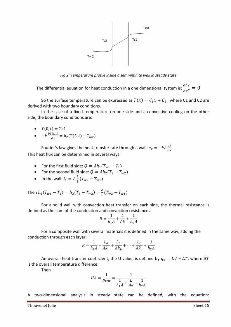
Heat conduction is considered in a semi infinite plane wall, under steady state conditions.
Thouvenel Julie Sheet 15
Fig 2: Temperature profile inside a semi-infinite wall in steady state
The differential equation for heat conduction in a one dimensional system is:
So the surface temperature can be expressed as , where C1 and C2 are derived with two boundary conditions.
In the case of a fixed temperature on one side and a convective cooling on the other side, the boundary conditions are:
Fourier’s law gives the heat transfer rate through a wall:
.
This heat flux can be determined in several ways:
For the first fluid side:
For the second fluid side:
In the wall:
Then
For a solid wall with convection heat transfer on each side, the thermal resistance is
defined as the sum of the conduction and convection resistances:
For a composite wall with several materials it is defined in the same way, adding the conduction through each layer:
An overall heat transfer coefficient, the U value, is defined by , where is the overall temperature difference.
Then
A two-dimensional analysis in steady state can be defined, with the equation:
Thouvenel Julie Sheet 16
Several methods are used to solve for the temperature such as the method of separation of variables or a finite difference method, which will not be described in this paper, because the idea is to understand the phenomena of heat conduction through a solid, and the one dimensional analysis is enough to get this idea. [8]
7. Transient conduction
Two major dimensionless numbers are used in the study of transient conduction:
The Fourier number is a dimensionless time representing the ratio of the heat conduction over the rate of thermal energy:
Where is the diffusivity of the material, t is the characteristic time and is the thickness through which conduction occurs in the material.
The Biot number represents the ratio of the heat transfer resistance inside and at the surface of a body:
Where h is the heat transfer coefficient, is the thickness through which conduction occurs in the material and k is the thermal conductivity of the material.
The differential equation for one dimensional heat conduction through a wall is:
This can be written in a non dimensional form as:
Where
is a dimensionless space variable and
is a dimensionless
temperature variable. [10] Several methods allow solving for transient heat conduction problem, such as the
lumped capacitance method which assumes a uniform temperature distribution through the object and which is applicable for .
The separation of variables is also used. For a plane wall, the problem can be considered as one dimensional if the height and
the width of the wall are large compared to the thickness. Constant physical properties of the wall and constant heat transfer coefficient are assumed.
Transient temperature charts exist for transient conduction through a plane wall. For example the Heisler charts represent the evolution of the central temperature for transient conduction in an infinite plane wall, an infinite cylinder and a sphere. [11]
Other charts show the temperature response of the front face of a plate with insulated back face after sudden exposure to a uniform-temperature convective environment.

Thouvenel Julie Sheet 17
These charts represent the evolution of a normalized temperature
, where To is
the initial temperature and Ta is the temperature of the convective environment, as a function of the Fourier number, depending on the Biot number.
A lot of graphs have then been studied for the evolution of the temperature under transient conduction; however graphs apply to a precise case and cannot be used for different shapes or boundary conditions.
8. Thermal mass
Thermal mass is really important in a building, and reflects its ability to store heat.
Material with good thermal mass can store the heat and release it after. It can allow some inertia against temperature variations. Thermal mass is more beneficial when the difference between day and night temperatures is quite high.
It is an important parameter to take into account for thermal comfort in a building, and it can reduce considerably the cooling and heating loads. For example in summer thermal mass absorbs the heat during the day and release it slowly at night so that cooling is reduced during the day and heating is not needed at night. Thermal mass has to be well placed and some parameters like coverings and colors can play a role on it. [12]
Materials with high specific heat capacity and high density are the best regarding thermal mass, since thermal mass can be seen as the volumetric heat capacity of a material.
Then if the volumetric thermal mass is noted it can be approximated with:
[13]
9. Laser flash analysis method
The laser flash method has been studied in 1961 by Parker et al., to measure the
diffusivity of various materials. The method consists of a laser which heats up one side of a parallel plate. Detectors
situated on the backside of the sample record the temperature evolution on this side. The sample is located in a furnace at constant temperature, since the diffusivity varies a lot with temperature. [15]
Fig 3: Scheme of the laser flash method
Some conditions for the experiment are that the material studied has to be considered
homogeneous, the experiment is a one-dimensional set up, and adiabatic boundaries are considered. Then the size of the sample is really small, which is not applicable in this work. [16]

Thouvenel Julie Sheet 18
The temperature distribution within an insulated material of uniform thickness L can be described (with the thermal diffusivity is expressed in ), according to Carslaw and Jaeger by:
If a heat impulse Q (in is imposed as an initial condition, and is absorbed in a
small depth g of the sample at the surface x=0, then the initial condition can be written:
C is the heat capacity in and is the density in . Then the temperature distribution becomes:
Since g is really small,
.
And then on the back surface the temperature can be determined:
If adiabatic conditions and one dimensional heat transfer are confirmed, the
temperature rise at the other side of the heated sample can be described:
Where is the temperature rise of the sample, for which the maximum value is , is the thermal diffusivity of the sample, is its thickness, and t is the time after the heat pulse. [18] The temperature evolution observed has the specific shape:
Fig 4: Temperature evolution recorded by the detector

Thouvenel Julie Sheet 19
For the particular value
, which correspond to the time for which the
sample has reached the half of the final temperature increase, the thermal diffusivity if the sample can be calculated with:
The laser flash method is nowadays used a lot for thermal conductivity measurements. The equipment allows achieving measures over a wide range of temperatures and different companies are in competition for the best performance. [14]
II. Theory and approach
1. Model presentation
The purpose of this paper is trying to determine the U value of a wall and its thermal
characteristics looking at the outside surface with an IR camera. Then the idea of the experiment is to test several materials of different characteristics
(conductivity, density, heat capacity) and record the evolution of the surface temperature with the IR camera.
The different results obtained can then allow drawing interesting conclusions.
For this purpose, an insulated box will be built, with 2,6 m length, 2,5m height and 2,1m depth. These dimensions are quite big so that it can be representative of a normal room.
As seen in the literature survey, the temperature difference between the ambient temperature and the wall under study has to be sufficient for the results to be visible on the IR camera.
Then a heater will deliver heat through the material, and the evolution of the surface temperature will be recorded.
The box will be built in polystyrene, since polystyrene has a low conductivity of
so it is a good insulated material. Then the heat delivered inside the box will not be lost to the environment.
In order to heat more the first surface than the entire box a smaller polystyrene box will be added against the front side, and a heater will be placed inside.
The box will be made of three layers of polystyrene everywhere, except on the front side. On this side only two layers of polystyrene will be added so that the third layer can be a layer of another material to study. The heater will be placed inside the box, against the front wall so that the heat will mostly spread on the front surface, which will be seen by the camera.
The first idea was to have the box in a cold chamber, so that the temperature of the room would be low and the box could be heated rapidly to have good resolution with the camera. However the cold chamber was already occupied with another experiment and the chamber free at that moment was not working.
However the box will be built inside this chamber with an average room temperature of 20 °C.

Thouvenel Julie Sheet 20
The method that is developed in this work is supposed to work on a normal building. For example in winter time the average building temperature is assumed to be about 20°C, the outside temperature is 0°C, and by applying even more heat on the surface (for example 40°C) and recording with the camera the temperature evolution on the outside would theoretically allow to determine some characteristics of the building wall.
Then the model will be set up so that it can be representative of such a case: the interior of the box will be heated 16°C more than the outside temperature and the small box against the front wall will be heated 16°C more than the box. 20°C more was not achievable because the polystyrene smelt burn and a higher temperature was difficult to obtain.
With a room temperature of 20 °C, the box will be heated to 36°C and the small box against the front wall will be heated to 52°C. Then similar temperature evolution can be experimented, even if the cold chamber does not work. For this purpose, not only one heater will be used, but three: one in the small box to apply heat against the front surface, and two others inside the big box to heat it 16°C more than the air temperature in the room. The type of heater chosen is described later.
2. Simulation
Before doing any experiment, some simulations have been performed on Comsol
Multiphysics 4.2a. Comsol Multiphysics is a finite element simulation software. It analyses and solves a lot
of different problems regarding various kinds of physics. Several choices of modules are proposed, covering a large range of physic problems.
The software is used to model the experiment that will be performed. It can help concerning the equipment required for the experiment, and get ideas of trends for the results that will be recorded by the camera.
a. Flat plate
The software has been discovered and tested first for simple cases. The first case
simulated is a flat plate in 2D, using the module heat transfer in solids, first in steady state and then in transient analysis.
The height is set up to be 20 meters, while the thickness is 0,15 m. The simulation is performed in 2D, and in 2D Comsol sets automatically the width to 1 meter. The height being really higher than the length and width, the model can be approximated to be close to a one dimensional plate, as referred in the literature survey.
Heat transfer in solids is the module chosen for this simulation. Several parameters for the material can be fixed: the heat capacity, the density and the conductivity.
The initial temperature is set to 60°C and the plate is cooled by natural convection. The heat transfer coefficient will be changed in order to simulate situations with different Biot
numbers
.
Both sides of the plate are cooled with the same heat transfer coefficient, so the problem can be symmetric, and the results can be similar to the curves obtained in the literature survey, where one side is cooled by natural convection and the other side is insulated.

Thouvenel Julie Sheet 21
However the thickness is then considered to be the half of the plate thickness, which is to say 0,075 m instead of 0,15m.
The evolution of the surface temperature is then run as a function of time. The varying
time will make the Fourier number changing also
.
A normalized temperature is set equal to:
Where Tini is the initial temperature of the plate (60°C in this case), and Ta is the temperature of the ambient which cools the plate (20°C).
This normalized temperature can be drawn as a function of the Fourier number, depending on the Biot number, curves similar to the ones seen in the literature survey. The Fourier number axis has a logarithmic scale. Different cases are tested: low Fourier numbers, low Biot numbers, high Fourier numbers, high Biot numbers, …
Fig 5a : Evolution of the temperature on the surface as a function of the Fourier number, for high
Biot numbers and low Fourier numbers
Fig 5b : Evolution of the temperature on the surface as a function of the Fourier number, for low Biot
numbers and high Fourier numbers

Thouvenel Julie Sheet 22
Fig 5c : Evolution of the temperature on the surface as a function of the Fourier number, for low Biot
numbers and low Fourier numbers
Fig 5d: Evolution of the temperature on the surface as a function of the Fourier number, for high
Biot numbers and high Fourier numbers
The curves obtained have a similar shape compared to the theoretical ones seen in the
literature survey. Then the simulation seems to be right and the software is better controlled. However the simulation seems correct since in each graph with different ranges of
Fourier and Biot numbers, the same normalized temperature and the same Biot number give the same Fourier number for each case.
Then a similar approach will be performed with not a flat plate any more, but the real
box that will be experimentally studied.
b. Influence of the edges
The theory based on is related to one dimensional heat transfer through a wall, so the wall is considered infinite.
In this case, the simulation is performed in two dimensions. The box is not infinite, however the height is huge compared to the thickness and the front wall could maybe approach the one dimensional theory so one might be interested of the results with such correlations.
One thing that differs is that the model is not symmetric any more since the convective cooling is not the same outside and inside the box.
Thouvenel Julie Sheet 23
Other things really different are the edges up and down that may influence the temperature profile on the front surface.
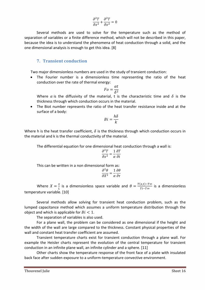
To see the influence of the edges, a simulation has been performed with just the front surface without the rest of the box.
i. Without edges
The conditions are the same: convective cooling with the exterior with a temperature
equal to 0°C, convective cooling on the interior with a temperature equal to 20°C. The bottom temperature is set equal to the floor temperature which is assumed to be the exterior temperature equal to 0 °C. The same small box is fixed to the surface, with the temperature set to 60°C to heat the box.
The simulation is performed in steady state, and then the temperature distribution obtained is computed as the initial condition for the transient analysis.
The simulation is tested with =500 kg/ , Cp=1500 J/kgK, and k=0.06 W/mK.
Fig 6: Simulation in transient without edges
A point is created at the center of the front surface (coordinates are x=0 and y=1,25). The temperature of this central point can be drawn in respect with time (see the result below).
ii. With edges
The first simulation with the entire box is performed again with the characteristics:
=500 kg/ , Cp=1500 J/kgK, and k=0.06 W/mK. The point at x=0 and y=1,25 m is created and the temperature profile of this point can be drawn also.

Thouvenel Julie Sheet 24
Fig 7: Simulation in transient with the edges
iii. Comparison
Fig 10 a-b: Central point temperature evolution, without edges (a) and with edges (b)
The temperature profiles of the two cases are really close. The temperatures are the same or slightly different so the presence of edges at the top and at the bottom of the front wall does not influence the temperature distribution at the middle of the wall.
Then it can be interesting to see the difference over the entire front surface. Another
point is created at x=0 and y=2,4 m. Then this point is situated very close to the top edge. The two cases are run again leading to the following result.
Fig 8 a-b: Central point temperature evolution (x=0 and y=1,25 m) first without edges (fig a) and then with edges (fig b)

Thouvenel Julie Sheet 25
The difference of temperature for this point is not negligible. The edges really influence
the temperature profile at a small distance, so the one dimensional approximation is not correct concerning the temperature of the entire surface.
However if one considers only the temperature at the center of the front wall then the approximation can perhaps be assumed. Then the temperature considered will be the central point temperature.
On Comsol, the box is tested: the first layer of the front surface is changed with several materials of different characteristics , Cp and k.
c. Insulated box
When the software has been more controlled, the insulated box is represented.
In Comsol Multiphysics, several modules can be chosen. After different tests, the heat transfer in solids seems to work the best for the simulation. The simulation is first run in steady state, as it is easier, and then in transient.
The box is constructed in 2 dimensions as it is easier to control than 3D and can be enough for the theory. The materials chosen are polystyrene for the big box and the box around the heater, air in the box where the heater is placed, and an unknown material for the first layer of the front side, with density, heat capacity and conductivity that can be changed. The polystyrene has been set with a density of 15,075 , a conductivity of 0,036 and a heat capacity of 1300 . The density has been calculated in the laboratory with the polystyrene received from the manufacturer. The heat capacity and the conductivity have been taken from literature.
The heat transfer in solids module is chosen. The initial temperature is set to 20 °C in the box. The exterior temperature is set to 0°C for the cooling of the box. Convective cooling is applied on the exterior of the box. The heat transfer coefficient is user defined so that the Biot number can be chosen. Another convective cooling is applied on the interior of the box with another heat coefficient defined by user. The temperature of the lower side of the box is assumed equal to the exterior temperature. A fixed temperature is set inside the small box to represent the heater.
Fig 9 a-b: temperature evolution for the point at x=0 and y=2,4 m first without edges (fig a) and then with edges (fig b)

Thouvenel Julie Sheet 26
As the box is built in polystyrene, it is better to work with a fixed temperature rather than a fixed power otherwise the polystyrene could burn or melt.
Fig 10: box in 2D in Comsol Multiphysics
i. Steady state
The model is meshed and run in steady state first. In steady state the theory says that
no heat is stored and all the heat that goes in the box goes out of the box. This verification can be done to see if the model can be considered correct.
Instead of setting the temperature on the small box, a heat source is placed inside this
box, with a power of 40 W. Then with Comsol one can know the total heat flux that passes through each wall. The
total heat flux that passes through the surfaces are 11,12 for surface 1, 1,88 for surface 2, 1,81 for surface 3, and 1,86 for surface 4.
Fig 11: Simulation in steady state
1
3
2
4
Heat source
IR camera
Material under study
, Cp, k
Polystyrene =15,075
kg/ Cp=1300 J/kgK K=0,036 W/mK

Thouvenel Julie Sheet 27
So the total heat loss through the surfaces of the box is:
The heat added into the small box is equal to the heat that leaves the box, so the simulation does not seem wrong at least for this point.
ii. Transient
The model is then computed depending on time. The box is the same as before. But one difference is that the steady state is first computed, and the surface distribution obtained is set to be equal to the initial condition of the transient state. Some graphs and correlations have been derived for a flat plate with convective cooling on both sides.
A similar approach can be tested on the front wall of the box. The heat flux is applied and the temperature evolution of a point situated on the middle
of the front surface (x=0 and y=1,25 m) is recorded for the different materials. For a particular combination of , Cp and k the simulation is run for different heat
transfer coefficients so different Biot numbers. The Fourier number changes as the time increases. The parameters are then changed to get curves for high Fourier number, low Fourier number, high Biot number and low Biot number to cover numerous different cases.
Some curves can be drawn, similar to the ones studied in the literature survey, of a
normalized temperature as a function of the Fourier number, depending on the Biot number. The normalized temperature is chosen as:
Where Ts is the surface temperature at the point measured and To is the initial temperature (20°C in this case).
Fig 12 a: Evolution of the temperature on the surface as a function of the Fourier number, for high
Biot numbers and high Fourier numbers

Thouvenel Julie Sheet 28
Fig 12 b: Evolution of the temperature on the surface as a function of the Fourier number, for low
Biot numbers and high Fourier numbers
Fig 12 c: Evolution of the temperature on the surface as a function of the Fourier number, for high
Biot numbers and low Fourier numbers
Fig 12 d: Evolution of the temperature on the surface as a function of the Fourier number, for low
Biot numbers and low Fourier numbers

Thouvenel Julie Sheet 29
Fig 12 e: Evolution of the temperature on the surface as a function of the Fourier number, for high
Biot numbers and medium Fourier numbers
Transient conduction depends most on the Fourier and the Biot numbers. Theoretically one graph should correspond to another one: for the same Biot number, the same normalized temperature should gives the same Fourier number, even if the parameters included in these numbers are not the same.
However in these graphs, it is not the case. Similar normalized temperatures do not have the same corresponding Fourier number in each graph. Then something must be wrong in the simulation, or some correction should be added for not having the same initial temperature profile in the wall; such correlations cannot be applied for the box that is in 3D and is not a one dimensional problem.
d. Ideas of a better model
Some things have been tested. However the model on Comsol is not precise enough to
give reliable correlations. A better model including convection and radiation inside the box should be performed in order to be able to deduce reliable results with only a simulation. Then another module was tried, giving heat transfer with conduction, convection and radiation.
Fig 13: Simulation taking into account convection and radiation
Thouvenel Julie Sheet 30
This picture gives an idea of what it could be. However the model is really difficult to be
run and a lot of errors appear. Such a model has not been totally finished and managed, because of too little time to deal with a new software, and correct all the errors. But this model tries to show a better representation of the air inside the box, and should be improved to be able to deduce results with more accuracy, using only the simulation.
Then, in the following of this work the model of heat transfer in solids in Comsol will be
used to get the trends and the idea of the heat required inside the box. However the results that will be taken into account will be those of the real experiment.
e. Estimation of the heat source required
The amount of heat necessary to heat up the box has to be determined in order to
choose the correct heater. The assumption that has been made for this first estimation is that the heat transfer in
the entire box is considered as heat transfer in solids. It is then an approximation of the heat required and not the real one, but it is accurate enough for an idea of the heater needed.
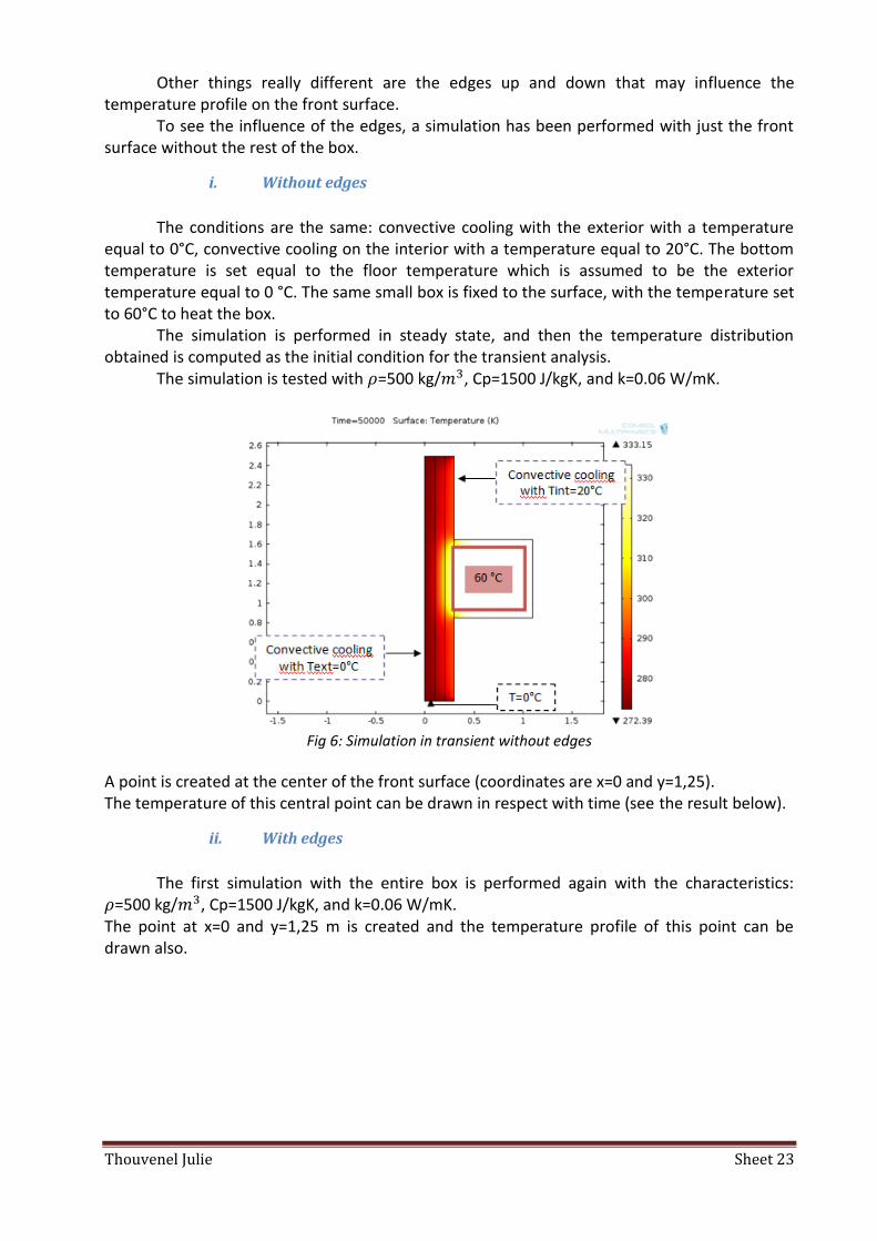
The heat transfer through a semi infinite plate or a plate which has a really bigger height than width can be approximated to be mono directional, and the heat flux in blue below can be calculated with:
Fig 14: Mono directional heat flow through each layer
Then the heat needed in the box could be calculated for each direction. However in reality the front layer of the box has a height of 2,5 meters and a thickness
of 0,3 meters, which is not negligible. So the heat flow cannot be calculated with this approximation because more heat will be dissipated.
Then to calculate more precisely the amount of heat needed in the box, the simulation in Comsol has been used in steady state. First the calculation has been made by hand with the mono directional hypothesis. The simulation has been run in Comsol and the result was higher. It can be logical since the 1D hypothesis is not justified in this case.
Then to be sure that one could be confident in the software, the front layer has been changed: instead of having a width of 0,3 meters, it has been changed to 1 centimeter. Then the width can be negligible compared to the height and the hypothesis of mono directional flux can be verified.
Thouvenel Julie Sheet 31
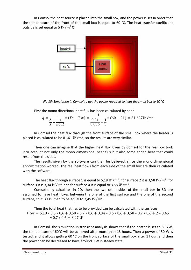
In Comsol the heat source is placed into the small box, and the power is set in order that the temperature of the front of the small box is equal to 60 °C. The heat transfer coefficient outside is set equal to .
Fig 15: Simulation in Comsol to get the power required to heat the small box to 60 °C
First the mono directional heat flux has been calculated by hand.
In Comsol the heat flux through the front surface of the small box where the heater is
placed is calculated to be 81,61 , so the results are very similar. Then one can imagine that the higher heat flux given by Comsol for the real box took
into account not only the mono dimensional heat flux but also some added heat that could result from the sides.
The results given by the software can then be believed, since the mono dimensional approximation worked. The real heat flows from each side of the small box are then calculated with the software.
The heat flux through surface 1 is equal to 5,18 , for surface 2 it is 3,58 , for
surface 3 it is 3,34 and for surface 4 it is equal to 3,58 . Comsol only calculates in 2D, then the two other sides of the small box in 3D are
assumed to have heat fluxes between the one of the first surface and the one of the second surface, so it is assumed to be equal to 3,45 .
Then the total heat that has to be provided can be calculated with the surfaces:
In Comsol, the simulation in transient analysis shows that if the heater is set to 8,97W,
the temperature of 60°C will be achieved after more than 13 hours. Then a power of 50 W is tested, and it allows getting 60 °C on the front surface of the small box after 1 hour, and then the power can be decreased to have around 9 W in steady state.

Thouvenel Julie Sheet 32
This simulation was a first approximation to know the type of heater to be used: the
conclusion is that a light bulb is enough to get the required temperature in the small polystyrene box.
A similar analysis has been performed to know which type of heater to use inside the big box. The result was the same: two light bulbs are enough to get around 36°C inside the big box.
3. Nodal method
In this work some relations related to one dimensional heat transfer analysis are used,
such as the nodal method to analyze the results given with the experiment.
a. Determining the wall characteristics knowing the heat transfer coefficient
A node can be considered at the surface, with convection and radiation boundary conditions:
Fig 16: node at the surface
(Source: John Richard Thome, Numerical techniques for conduction, March 2010, EPFL)
At this node, an energy balance can be done, giving:
In this case, Tin is the imposed temperature:
Then the temperature of the time t+1 can be deduced from the temperature of the time t with:
Thouvenel Julie Sheet 33
i. Heat transfer coefficient
If the formula is entered in Excel with these parameters, the unknown is the heat
transfer coefficient h because in the experiments the properties of the material tested will be known.
The temperatures at the time t+1 can be calculated from the first temperature given by the camera, depending on the h value.
Then the coefficient h, which is the only unknown in this equation, can be adjusted until the curve of the temperatures calculated fits perfectly the curve of the temperatures obtained with the experiment.
Knowing the heat transfer coefficient will lead to the determination of the material’s conductivity.
ii. Conductivity
The heat going out of the front surface will be estimated for the region where the measurement is stable (when the imposed temperature and the exterior temperature can be assumed constant):
An average of these heats deduced from each measurement will be calculated over the
entire range of the stable state. An average surface temperature will also be calculated for the same range of time. It leads to more accurate value since the temperatures in the stable region are supposed to be constant.
Then the thermal conductivity of the material is deduced with:
iii. U value
In theory, the U value can be calculated with:
Where Rsi is the resistivity of air on the inside surface, Rse is the resistivity of air on the
outside surface and are the resistivity of each material. Knowing the heat transfer coefficients on the inside and outside one can determine the
resistivities Rsi and Rse, and knowing the thicknesses and conductivities one can deduce the resistivities
Then

Thouvenel Julie Sheet 34
iv. Thermal mass
One parameter which could be interesting to deduce is the thermal mass. Two methods
are proposed to determine the thermal mass of the wall.
a. First method
The first uses the same formula below, this time knowing the temperatures, the heat
transfer coefficient and the conductivity.
Supposing that the conductivity k has been found with the method described before, now is the unknown, whereas the camera allows measuring
and .
Two constants appear in the equation:
The temperatures will be measured with the camera and placed in the first column. The temperature will then be calculated with the formula with the two constants that can change. The software calculates
Where x is the matrix of the temperatures measured and y is the matrix of the temperatures calculated. Then this value is minimized with C1 and C2 as the variables with the tool solver.
The minimized value corresponds to the point for which the curves
measured and calculated are the closest, giving a combination of C1 and C2.
b. Second method
The second method is tougher and longer, but could also work without knowing the
conductivity k. The power introduced in the small box is regulated so that it keeps the temperature
constant in this small box to 52°C. It is regulated with a transformer that delivers a certain percentage of the total power. Then the power of the light bulb in the small box is known at every time.
But the heat that goes on the front surface has to be known to be able to deduce the characteristics of the front wall. Then the heat losses through the other sides of the small box have to be estimated.
The heat that goes out of the small box can be estimated for each side with:

Thouvenel Julie Sheet 35
Where is the heat transfer coefficient, A is the area of the wall, is the temperature of the exterior surface, is the ambient temperature and is the temperature of the surroundings.
But some heat is also stored in the walls of the small box. This heat can be estimated with:
Where and are the known density and heat capacity of polystyrene since the small box is built in this material, V is the volume of the wall considered, is the temperature difference of the volume considered for the time interval . For the temperature of the volume, the mean value between the exterior and interior temperatures is calculated.
Then the heat that goes through the first layer can be estimated as the total power introduced in the small box reduced by the heat losses through the five other walls of the small box and the five heats stored in these walls:
The heat loss through the front wall can be known with the IR camera evaluating the
front surface temperature:
Then with , the heat stored in the front layer can be
estimated also, with one thermocouple measuring the interior temperature of the wall.
Where V is the volume of the front wall considered, is the temperature difference of the front surface for the time interval , and and are the unknown material characteristics of the front wall.
Then with these approximations it would be possible to estimate the thermal mass of the unknown material:
To get a higher accuracy, mean values over a range of measurements (for example 10
measurements) will be calculated. Then these mean values will be used in the calculations, for
example to calculate
the difference will be made between two mean values, each one
regrouping ten values of the experiment.
b. Heterogeneous wall
To be able to calculate the heat transfer coefficient at the surface, a thermocouple will
be placed between the two layers. Then the same method than for a homogeneous wall is performed to get the heat transfer coefficient (the interior temperature in this case being the temperature measured between the two layers).

Thouvenel Julie Sheet 36
When the coefficient h is computed, the heat going out of the front surface is calculated as before:
In theory the effective conductivity of a heterogeneous wall could be calculated as:
The U value of the wall would be:
In this work the heat is calculated for all the points over the stable region and then an
average value of these heats obtained is deduced. Then the effective conductivity of the wall can be determined over the stable region as:
The U value will be calculated in the same way as for a homogeneous wall, using this
effective conductivity:
c. Determining the wall characteristics without knowing the heat transfer
coefficient
The method described before took into account that the heat transfer coefficient was
known, or preliminary deduced. In reality this coefficient will not be known most of the times. The coefficient could
maybe be deduced from literature but it will not be very accurate for the real case. The heat transfer coefficient inside a normal house is a value which does not vary a lot
and is usually known. Then this value is not the most difficult to deduce. The U value has been calculated for some fixed parameters ( hin, k) while varying the
exterior heat transfer coefficient.
Thouvenel Julie Sheet 37
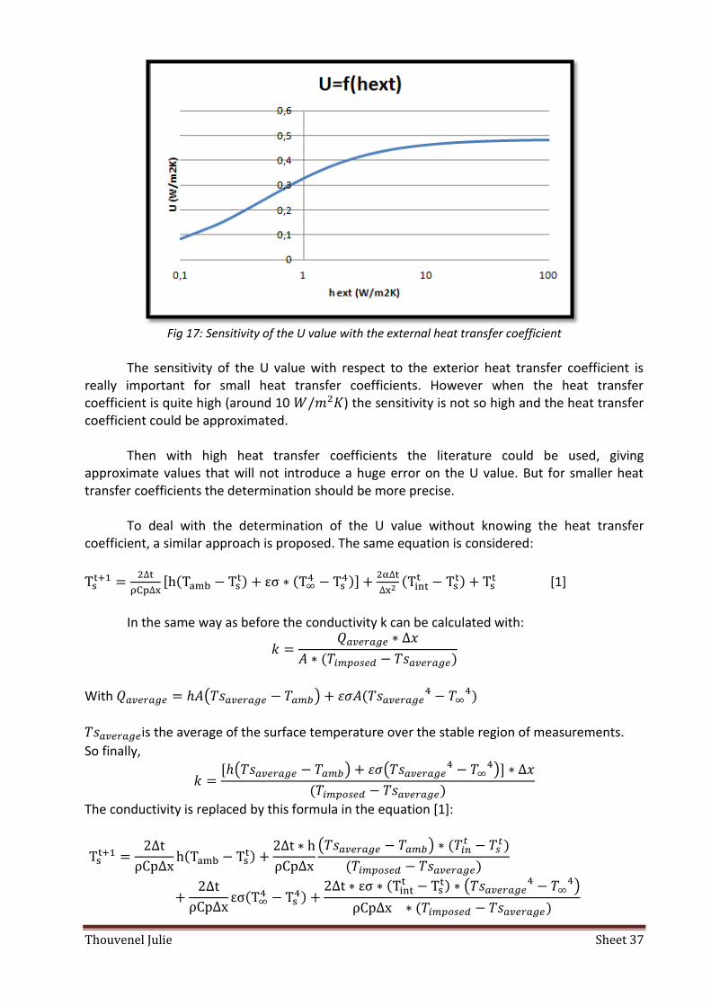
Fig 17: Sensitivity of the U value with the external heat transfer coefficient
The sensitivity of the U value with respect to the exterior heat transfer coefficient is
really important for small heat transfer coefficients. However when the heat transfer coefficient is quite high (around 10 ) the sensitivity is not so high and the heat transfer coefficient could be approximated.
Then with high heat transfer coefficients the literature could be used, giving
approximate values that will not introduce a huge error on the U value. But for smaller heat transfer coefficients the determination should be more precise.
To deal with the determination of the U value without knowing the heat transfer coefficient, a similar approach is proposed. The same equation is considered:
[1]
In the same way as before the conductivity k can be calculated with:
With
is the average of the surface temperature over the stable region of measurements.
So finally,
The conductivity is replaced by this formula in the equation [1]:
Thouvenel Julie Sheet 38
If the heat transfer coefficient and the conductivity are not known, two constants appear in the equations:
So the temperatures measured with the camera could be used to deduce first the
thermal mass with the second constant and then the heat transfer coefficient with the first constant.
In Excel the temperatures measured will be placed in the first column. The temperature will then be calculated with the formula with the two constants that can change. The software calculates
Where x is the matrix of the temperatures measured and y is the matrix of the temperatures calculated. Then this value is minimized with C1 and C2 as the variables with the tool solver.
The minimized value corresponds to the point for which the curves measured
and calculated are the closest, giving the combination C1 and C2.
III. Experimental study
1. Construction of the box
The box presented earlier in this paper has been built. The plans have been done for the
box to be built, and are represented in the annex (see annex A1).
Some thermocouples are added on the box to study the overall temperature evolution, and compare some temperatures with the camera.
One thermocouple is placed at the middle of each surface of the box:
Surface Left side Back side Right side Top Bottom
Thermocouple 3 5 9 12 15 Table 1: Thermocouples on the interior surfaces of the big box
Some thermocouples are placed in the box to measure the air temperature:
thermocouples 2,4,7 and 13. To measure the heat fluxes through the small box heating the front surface,
thermocouples are placed on the interior and on the exterior surfaces of this small box:
Thouvenel Julie Sheet 39
Interior Surface of the
small box
Left side Back side Right side Top Bottom
Thermocouple 17 19 22 24 21 Exterior
Surface of the small box
Left side Back side Right side Top Bottom
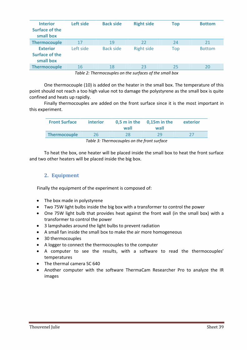
Thermocouple 16 18 23 25 20 Table 2: Thermocouples on the surfaces of the small box
One thermocouple (10) is added on the heater in the small box. The temperature of this
point should not reach a too high value not to damage the polystyrene as the small box is quite confined and heats up rapidly.
Finally thermocouples are added on the front surface since it is the most important in this experiment.
Front Surface interior 0,5 m in the wall
0,15m in the wall
exterior
Thermocouple 26 28 29 27 Table 3: Thermocouples on the front surface
To heat the box, one heater will be placed inside the small box to heat the front surface
and two other heaters will be placed inside the big box.
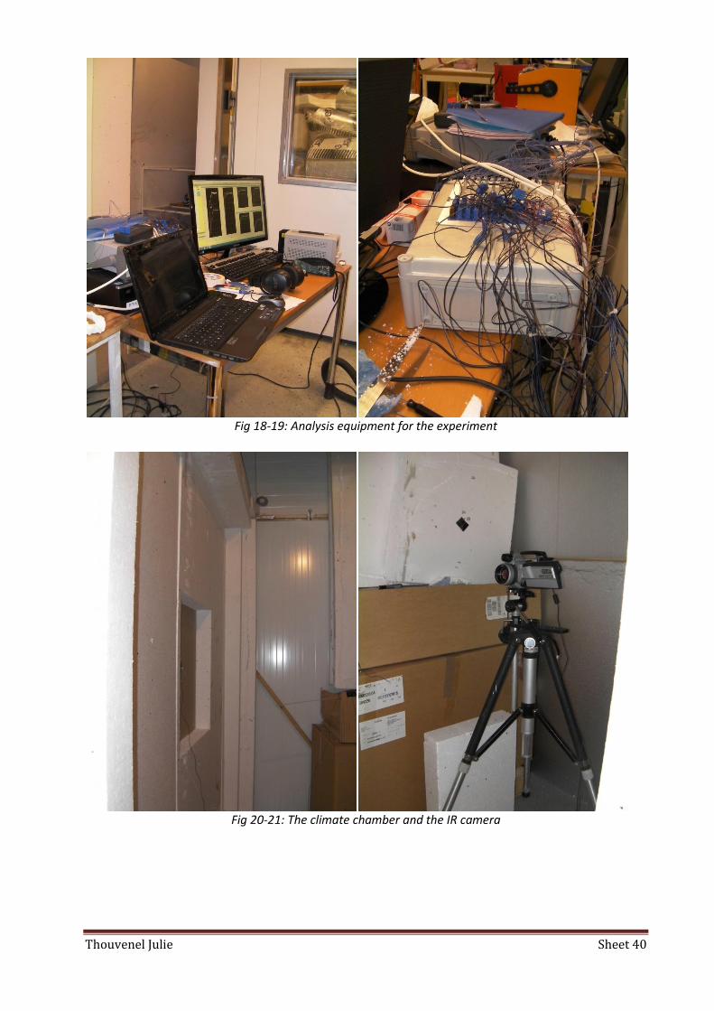
2. Equipment
Finally the equipment of the experiment is composed of:
The box made in polystyrene
Two 75W light bulbs inside the big box with a transformer to control the power
One 75W light bulb that provides heat against the front wall (in the small box) with a transformer to control the power
3 lampshades around the light bulbs to prevent radiation
A small fan inside the small box to make the air more homogeneous
30 thermocouples
A logger to connect the thermocouples to the computer
A computer to see the results, with a software to read the thermocouples’ temperatures
The thermal camera SC 640
Another computer with the software ThermaCam Researcher Pro to analyze the IR images
Thouvenel Julie Sheet 40
Fig 18-19: Analysis equipment for the experiment
Fig 20-21: The climate chamber and the IR camera
Thouvenel Julie Sheet 41
3. Preliminary experiments
a. Initial adjustment
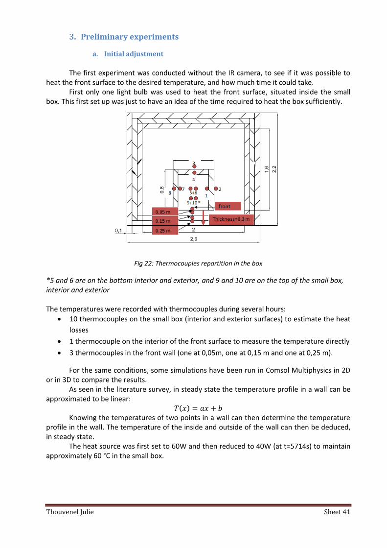
The first experiment was conducted without the IR camera, to see if it was possible to heat the front surface to the desired temperature, and how much time it could take.
First only one light bulb was used to heat the front surface, situated inside the small box. This first set up was just to have an idea of the time required to heat the box sufficiently.
Fig 22: Thermocouples repartition in the box
*5 and 6 are on the bottom interior and exterior, and 9 and 10 are on the top of the small box, interior and exterior The temperatures were recorded with thermocouples during several hours:
10 thermocouples on the small box (interior and exterior surfaces) to estimate the heat
losses
1 thermocouple on the interior of the front surface to measure the temperature directly
3 thermocouples in the front wall (one at 0,05m, one at 0,15 m and one at 0,25 m).
For the same conditions, some simulations have been run in Comsol Multiphysics in 2D or in 3D to compare the results. As seen in the literature survey, in steady state the temperature profile in a wall can be approximated to be linear:
Knowing the temperatures of two points in a wall can then determine the temperature
profile in the wall. The temperature of the inside and outside of the wall can then be deduced, in steady state. The heat source was first set to 60W and then reduced to 40W (at t=5714s) to maintain approximately 60 °C in the small box.

Thouvenel Julie Sheet 42
i. Results
Fig 23 a-b: Temperatures recorded on the surfaces of the small box (interior and exterior)
Fig 24a: temperatures recorded on the front surface fig24 b: temperatures recorded and calculated
with the steady state formula
ii. Analysis
The temperatures inside the small box evolve in the same way so the air can be
considered homogeneous in the small box. The thermocouples on the bottom interior surface, on the top interior surface and on the right interior surface do not work properly. The exterior surface temperatures also does not seem to work well, only the left side temperature seems correct since it evolves the same way as the other temperatures.
The time required to heat the interior of the small box to 60 °C is about 85 min.
This evolution is not satisfactory since the interior of the box has first the same temperature than the exterior. As the thickness of the small box is 0,1m and the thickness of the front layer is 0,3m, more heat will flow in the box than in the front layer. To simulate a real case of a house in winter that has an inside temperature of 20°C superior than the ambient temperature, two other light bulbs are added inside the box to heat it to 40°C.
0 10 20 30 40 50 60 70 80
0 100 200 300
T (°
C)
time (min)
Interior surface temperatures, small box
t1 left int
t4 back int
t6 bottom int
t7 right int
t9 top int
t11 front int 0
10 20 30 40 50 60 70 80
0 100 200 300
T (°
C)
time (min)
Exterior surface temperatures, small box
t2 left ext
t3 back ext
t5 bottom ext
t8 right ext
t10 top ext
0
20
40
60
80
0 100 200 300
Titr
e d
e l'
axe
Titre de l'axe
Front surface temperatures
t11 front int
t28 (0,05)
t29 (0,15)
t30 (0,25) 0
20
40
60
80
100
120
0 2000 4000 6000
T (°
C)
time (min)
Tfront simulated and experiment for P=60W
t11 front int
T (3d model)
T calculated
T (2D model)
T2D small source

Thouvenel Julie Sheet 43
b. Additional adjustments
The experiment is run again with three light bulbs inside the box. Two light bulbs will heat the inside of the box to 40°C and one light bulb will heat the small box and the front layer to 60°C.
More thermocouples are added. Three thermocouples on each surface of the big box measure the temperature of the inside surface, at 0,15m in the wall and at 0,25m in the wall.
Fig 25: New placement of the thermocouples: the purple ones are added.
In the middle the 6 points represent the thermocouples of the top surface and the bottom surface.
i. Results
Fig 26-27: Temperatures of the back side and the left side of the box recorded and calculated with the steady state formula
0
10
20
30
40
50
0 20 40 60
Titr
e d
e l'
axe
Titre de l'axe
Back side big box
t4 (0,25 back)
t5 (surf back)
t6 0,15 (back)
T back calcul 0
10
20
30
40
0 20 40 60
Titr
e d
e l'
axe
Titre de l'axe
Left side big box
t1 (0,15 left)
t2 (0,25 left)
t3 (surf left)
T surf left calculated

Thouvenel Julie Sheet 44
Fig 28-29: Temperatures of the right side and the bottom of the box recorded and calculated with the steady state formula
Fig 30: Temperatures of the top of the box recorded and calculated with the steady state formula
ii. Analysis
The interior temperatures of the big box seem to have the same evolution, except from
the right side. It can come from the fact that the right surface is farer from the light bulbs than the other surface, but most probably that the thermocouples do not work properly.
When the power is increased, an increase in the temperature is instantaneously recorded. However some delay should be noticed. This can reveal that radiation inside the box between the light bulbs and the surfaces is too high to be negligible and interferes in the temperature measurement. Then the temperature measured is the radiated temperature and not the real one.
The comparison of the surface temperatures revealed that the temperatures calculated with the steady state approximation (based on two temperatures inside the wall) do not work in this case, it is not even close. This is logical since the experiment is done in transient.
Then the thermocouples inside the walls will be placed at other places, and the temperature that will be believed is the temperature given by the thermocouples on the surfaces: radiation and other phenomenon that can interfere with these temperatures have to be minimized.
To see if the temperature is homogeneous in the big box so that one can assume the surface temperatures of the big box to be equal everywhere, some thermocouples will be placed in order to measure the air inside the big box at different places.
0
5
10
15
20
25
30
0 20 40 60
Titr
e d
e l'
axe
Titre de l'axe
Right side big box
t7 (0,25 right)
t8 (0,15 right)
t9 (surf right)
T right calcul 0
10
20
30
40
0 20 40 60
Titr
e d
e l'
axe
Titre de l'axe
Bottom big box
t13 (0,25 bottom)
t14 (0,15 bottom)
t15 (surf bottom)
T bottom calcul
0
20
40
60
80
0 20 40 60
Titr
e d
e l'
axe
Titre de l'axe
Top big box
t10 (0,25 top)
t11 (0,15 top)
t12 (surf top)
T top calcul

Thouvenel Julie Sheet 45
This experiment mainly showed that something was wrong with some thermocouples and that radiation was a problem to get rid of.
The thermocouples have been made by hand. The problem was that the steel wire and the copper wire touched before being connected to the logger, and the potential difference did not reveal the correct temperature. All the incorrect thermocouples were then modified.
Fig 31: Thermocouple
Some lampshades were added around the light bulbs to minimize the radiation effect. These lampshades are made of gold copper so that it does not burn even if it is really close to the light bulb.
iii. Correction
Then the simulation has been run again with the lampshades.
Fig 32-33: Temperature evolution of the air inside the box and temperature evolution of the surfaces of the big box
Fig 34-35: Temperature evolution of the interior surfaces of the big box and temperature evolution of the front surface
0
10
20
30
40
50
0 200 400 600
T (°
C)
time (min)
T air box
t2 (air left)
t4 air back
t7 air right
t13 air bottom 0
10
20
30
40
50
0 200 400 600
T (°
C)
time (min)
T surface big box
t3 surf left
t5 surf back
t9 surf right
t12 surf top
0
10
20
30
40
50
60
0 200 400 600
T (°
C)
time (min)
Surface interior small box
t17 left int small
t19 back int small
t21 bottom int small
t22 right int small
0
10
20
30
40
50
60
0 200 400 600
T (°
C)
time (min)
Front surface
t26 front int
t27 front ext
t28 front 0,05
t29 front 0,15
t30 front 0,25
The wires were in contact
before the blue holder

Thouvenel Julie Sheet 46
Fig 36: Temperature evolution of the exterior front surface
The experiment shows that the air temperatures measured inside the big box are similar, so one can guess that the air is homogeneous inside the box, giving the same temperatures to the surfaces of the big box. Thermocouple for the right surface has fallen which explains its different values, so this thermocouple is not considered in this experiment. The exterior front surface temperature has some sudden changes, which are due to people entering in the room during the experiment, changing the surface temperature for a few seconds.
When setting the power inside the small box, smell of burned appeared at high temperatures. To reach 60°C inside the small box was not possible with the set up, polystyrene smell bad. Then a thermocouple has been added on the lampshade, so directly on the heat source, and this temperature will be controlled also.
For the temperature difference to be kept, the small box will be heated only sixteen degrees more than the outside temperature, and the small box sixteen degrees higher than the big box, so for an ambient temperature of 20 °C, the big box is heated to 36°C and the small box to 52°C. Finally even if the front surface temperature increases while increasing the temperature inside the small box, the increase is not really significant: it gains one degree in at least five or six hours so the results are not really exploitable. Then one layer of polystyrene will be removed from the front.
After these first experiments without camera, the time and the power needed to increase the temperature of the front surface to 52°C is known. For the next experiments, the big box will be heated first, and then the power in the small box will be started.
4. IR camera experiments on polystyrene
The software needed to interpret the IR camera’s images is installed. The camera used
for the experiments is a Flir system camera, model SC 640. The camera is positioned approximately one meter far from the front wall of the box
and the parameters are entered, like the object distance or the reflected temperature. The ambient temperature is measured to be equal to 19°C. Then the power is set into
the big box to heat it to 35 °C. To set the emissivity of the material in the object parameters of the camera, the
temperature is seen on the camera and measured with a thermocouple. The emissivity of 0,95
19,5
20
20,5
21
21,5
22
22,5
0 200 400 600 T
(°C
) time (min)
t27 front ext
t27 front ext

Thouvenel Julie Sheet 47
was set to obtain the same temperature (after correction), which seems to be in a correct range since the polystyrene is a material close to the blackbodies, its emissivity is close to 1.
When the temperature inside the big box has reached 35°C, the light bulb in the small box is turned on with a constant power (45W) and then reduced when the temperature reaches 50°C to keep it stable.
a. Results
The camera recorded the temperatures of a central area of the front surface every two
minutes. Thermocouples were still placed inside the box to control the imposed temperatures.
Fig 37-38: Temperature evolution of the air inside the box and temperature evolution of the surfaces of the big box
Fig 39-40: Temperature evolution of the interior surfaces of the big box and temperature evolution of the front surface
The evolution of the central temperature of the front surface recorded with the camera
can be seen as an addition of pictures with the software ThermaCam researcher, but only the first and last pictures are presented below, with the same scale of temperatures.
There is no color contrast on one single picture since the area recorded is situated on the heated surface, and the temperature does not vary a lot between two points. However if the temperature scale is set equal for all the pictures, then watching the images successively as a film allows to see the color differences.
0
10
20
30
40
0 200 400 600
T (°
C)
time (min)
T air big box
t2 air left
t4 air back
t7 air right
t13 air bottom 0
10
20
30
40
0 200 400 600
T (°
C)
time (min)
T surface big box
t3 surf left
t5 surf back
t9 surf right
t12 surf top
0
10
20
30
40
50
60
0 200 400 600
T (°
C)
time (min)
Interior small box
t17 left int
t19 back int
t21 bottom int
t22 right int
t24 top int
t26 front int
0
10
20
30
40
50
60
0 200 400 600
T (°
C)
time (min)
T front wall
t26 front int
t27 front ext
t28 0,05 front
t29 0,15 front

Thouvenel Julie Sheet 48
Fig 41-42: Thermal images at the beginning and at the end of the experiment
The temperature evolutions recorded with the camera and with the thermocouple were
compared. The emissivity was set to 0,8 first and the reflected temperature was set to 21 °C.
Fig 43: Comparison between the temperatures measured by the camera and the temperatures given by
the thermocouple
The temperatures are close but it seems to have a difference between the curves. If the temperature measured with the camera is lowered with 0.5 °C (probably because of a small mistake in the selection of the object parameters in the camera set up and because of the thermocouple precision), the curves seem to fit.
Nevertheless the emissivity has been corrected first to have the same temperature given by the camera and by the thermocouple, which is visible on the graph above: at the beginning the temperatures are closer than at the end.
But the thermocouple was fixed with a black tape. The camera has been set up on the central point, so the black tape could interfere in the settings because its emissivity is different. Moreover it was difficult to set the camera and control the temperature given by the thermocouple at the same time.
Then the parameters entered in the camera should be determined carefully at the beginning of the experiment. To get an accurate value, the camera is pointing not on the thermocouple point because black tape is used to fix the thermocouple, but the camera is set up taking into account the temperatures around the black tape.
To get more accuracy a correction is applied with ThermaCam Reasercher, because setting the parameters perfectly at the beginning of the experiment was not easy.
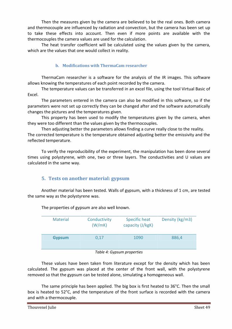
Thouvenel Julie Sheet 49
Then the measures given by the camera are believed to be the real ones. Both camera and thermocouple are influenced by radiation and convection, but the camera has been set up to take these effects into account. Then even if more points are available with the thermocouples the camera values are used for the calculation.
The heat transfer coefficient will be calculated using the values given by the camera, which are the values that one would collect in reality.
b. Modifications with ThermaCam researcher
ThermaCam researcher is a software for the analysis of the IR images. This software
allows knowing the temperatures of each point recorded by the camera. The temperature values can be transferred in an excel file, using the tool Virtual Basic of
Excel. The parameters entered in the camera can also be modified in this software, so if the
parameters were not set up correctly they can be changed after and the software automatically changes the pictures and the temperatures given.
This property has been used to modify the temperatures given by the camera, when they were too different than the values given by the thermocouples.
Then adjusting better the parameters allows finding a curve really close to the reality. The corrected temperature is the temperature obtained adjusting better the emissivity and the reflected temperature.
To verify the reproducibility of the experiment, the manipulation has been done several times using polystyrene, with one, two or three layers. The conductivities and U values are calculated in the same way.
5. Tests on another material: gypsum
Another material has been tested. Walls of gypsum, with a thickness of 1 cm, are tested the same way as the polystyrene was. The properties of gypsum are also well known.
Material Conductivity (W/mK)
Specific heat capacity (J/kgK)
Density (kg/m3)
Gypsum 0,17 1090 886,4
Table 4: Gypsum properties
These values have been taken from literature except for the density which has been
calculated. The gypsum was placed at the center of the front wall, with the polystyrene removed so that the gypsum can be tested alone, simulating a homogeneous wall.
The same principle has been applied. The big box is first heated to 36°C. Then the small
box is heated to 52°C, and the temperature of the front surface is recorded with the camera and with a thermocouple.
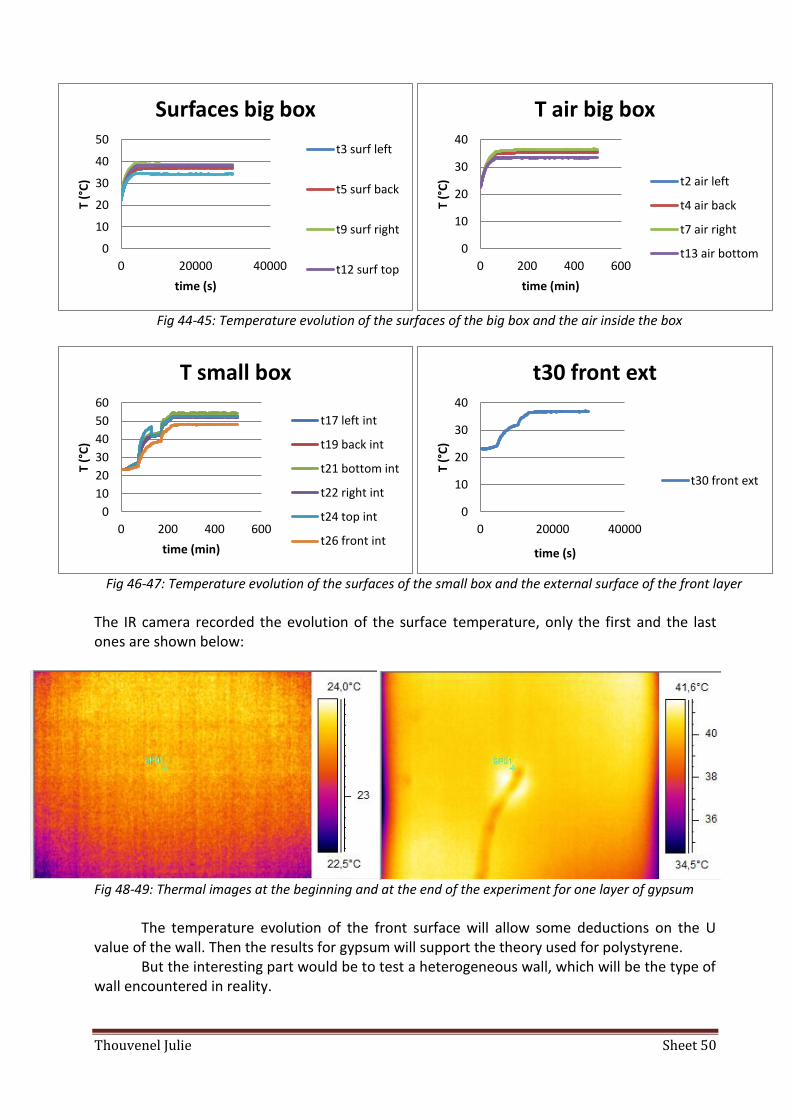
Thouvenel Julie Sheet 50
Fig 44-45: Temperature evolution of the surfaces of the big box and the air inside the box
Fig 46-47: Temperature evolution of the surfaces of the small box and the external surface of the front layer
The IR camera recorded the evolution of the surface temperature, only the first and the last ones are shown below:
Fig 48-49: Thermal images at the beginning and at the end of the experiment for one layer of gypsum
The temperature evolution of the front surface will allow some deductions on the U value of the wall. Then the results for gypsum will support the theory used for polystyrene.
But the interesting part would be to test a heterogeneous wall, which will be the type of wall encountered in reality.
0
10
20
30
40
50
0 20000 40000
T (°
C)
time (s)
Surfaces big box
t3 surf left
t5 surf back
t9 surf right
t12 surf top
0
10
20
30
40
0 200 400 600
T (°
C)
time (min)
T air big box
t2 air left
t4 air back
t7 air right
t13 air bottom
0
10
20
30
40
50
60
0 200 400 600
T (°
C)
time (min)
T small box
t17 left int
t19 back int
t21 bottom int
t22 right int
t24 top int
t26 front int
0
10
20
30
40
0 20000 40000
T (°
C)
time (s)
t30 front ext
t30 front ext

Thouvenel Julie Sheet 51
6. Experiments on a heterogeneous wall
After testing only homogeneous walls with one material, a heterogeneous wall consisting of layers of polystyrene and gypsum was tested.
The parameters of the materials are recalled below:
Material Conductivity (W/mK) Specific heat capacity (J/kgK)
Density (kg/
Gypsum 0,17 1090 866,4 Polystyrene 0,036 1300 22,2
Table 5: Material properties
The experiment shown below consists of one layer of gypsum with a thickness of 0,01 m and one layer of polystyrene of 0,03 m.
The same thermocouples as before measured the temperatures inside the big box,
inside the small box and at the surface of the wall. The IR camera was calibrated and recorded pictures every two minutes.
The results of the thermocouple on the exterior surface and the camera were compared.
Fig 50: Temperatures given by the camera and the thermocouple
The parameters were corrected using ThermaCam Researcher to get more accurate
values, calibrating the camera so that the first temperatures are the same with the camera and the thermocouple around the black tape.
The parameters used are those of polystyrene as the last layer is polystyrene (the one in contact with the air). So and are the values of polystyrene and is the thickness of only the last layer.
Several experiments have been done. The conductivity and the U value will be
compared with the theoretical value for each experiment.

Thouvenel Julie Sheet 52
IV. Interpretation of the results
1. Parameters identification
If the Nodal method is used, the temperatures can be expressed with:
a. Heat transfer coefficient
If the material properties are known, adjusting the curve of the temperatures calculated
and the curve of the temperatures obtained with the experiment, the coefficient of heat transfer h can be found. The first experiment is showed below, leading to a heat transfer coefficient equal to 2,4 .
Fig 51: Temperatures measured and calculated giving the real value of the heat transfer coefficient
b. Conductivity
Two calculations are made to calculate the conductivity:
One taking into account the temperature of the central point given by the camera, assumed representative of the total surface heated with an area of 0,6*0,6 .
One taking an average temperature of a certain area measured by the camera, taking this area into account in the calculations and not the total heated area. Then the thermal conductivity of the material is deduced with:

Thouvenel Julie Sheet 53
c. U value
As seen in the theory part, the U value can be calculated, after determining the heat
transfer coefficient and the conductivity:
This value will be compared to the theoretical one.
d. Thermal mass
The second method described in the theory part does not give reliable results, so the
first method is tested, taking the equation below:
With the two constants:
The software is used to find the two constants for which the curves of the temperatures
measured with the camera and the temperatures calculated with the formula are the closest.
The thermal mass can be deduced from the determination of the conductivity or with the heat transfer coefficient.
e. Without knowing the heat transfer coefficient
The equation changes if the heat transfer is supposed unknown:
With the two new constants:

Thouvenel Julie Sheet 54
The software is used to deduce the best combination of the two constants so that the curves of the temperatures measured and calculated are the closest.
Then the thermal mass can be deduced first with the second constant and then the heat transfer coefficient with the first constant.
2. Homogeneous wall
a. Material: polystyrene
The conductivities and U values found for the experiments on polystyrene are shown in
the table below:
Conductivity k (W/mK)
Experiment h (W/m2K)
Tamb (°C)
With T center
error With Tmean
error
1 2 layers polystyrene 2,4 19,7 0,037169 3,25 % 0,034048 5,42 %
2 3 layers polystyrene 1,9 19,3 0,036138 0,38 % 0,035822 0,49 %
3 2 layers polystyrene 2,2 20,8 0,035038 2,67 % 0,035571 1,19 %
4 2 layers polystyrene 3,5 21 0,035337 1,84 % 0,044433 23,4 %
5 2 layers polystyrene 2,5 19 0,036197 0,55% 0,039052 8,48 %
6 1 layer polystyrene 3 22 0,037284 3,57 % 0,034428 4,37 %
Material h ext (W/m2K)
h int (W/m2K)
Tamb (°C)
U value (W/m2K)
Using T central (A=0,6*0,6 )
Error compared with real value
1 2 layers polystyrene
2,4 5,75 19,7 0,167465 2,8 %
2 3 layers polystyrene
1,9 1,24 19,3 0,104 0,33 %
3 2 layers polystyrene
2,2 3,82 20,8 0,156 2,37 %
4 2 layers polystyrene
3,5 3,19 21 0,160 1,67 %
5 2 layers polystyrene
2,5 4,20 19 0,162 0,49 %
6 1 layer polystyrene
3 3,12 22 0,300 2,87 %
Table 6: Conductivities and U values obtained with other experiments
The experiments give all values for the conductivity really close to the real one (k=0,036 W/mK).

Thouvenel Julie Sheet 55
Moreover the real value of the polystyrene used might be slightly different than 0,036 W/mK since this value has been found in the literature. Properties are well defined for polystyrene so one can guess the real value to be this one, but small deviations can be possible. The results for the thermal mass are:
Thermal mass (J/kgK)
h (W/m2K)
Tamb (°C)
deduced with h
Error deduced with k
Error
1 2 layers polystyrene
2,4 19,7 20006,7 2,1% 19666,1 0,35 %
2 3 layers polystyrene
1,9 19,3 77506,1 295 % 20731,8 5,79 %
3 2 layers polystyrene
2,2 20,8 19904,9 1,57 % 18719,6 4,48%
4 2 layers polystyrene
3,5 21 19929,3 1,69 % 20426,0 4,23 %
5 2 layers polystyrene
2,5 19 19231,2 1,87 % 18852,6 3,80 %
6 1 layer polystyrene
3 22 20181,6 2,98 % 18099,0 7,65 %
Table 7: Thermal mass deduced from the experiments
The real value of is 19597,5 so some values obtained for the experiments
are quite close to the reality. However this method is not really accurate since the first guessed values must be really
close to the real ones, otherwise the solver does not give reliable results. So in the case of a totally unknown material it seems difficult to have a first guess of high accuracy.
Moreover the thermal mass obtained is not a precise number but an idea of the value,
since determining it with the heat transfer coefficient or the conductivity does not lead to the same result.
b. Material: gypsum
Another wall is tested to verify the results on a different material. The results are shown
in the tables below, with the same calculations as before.
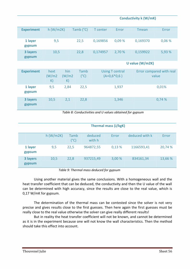
Thouvenel Julie Sheet 56
Conductivity k (W/mK)
Experiment h (W/m2K) Tamb (°C) T center Error Tmean Error
1 layer gypsum
9,5 22,5 0,169856 0,09 % 0,169370 0,06 %
3 layers gypsum
10,5 22,8 0,174957 2,70 % 0,159922 5,93 %
U value (W/m2K)
Experiment hext (W/m2
K)
hin (W/m2
K)
Tamb (°C)
Using T central (A=0,6*0,6 )
Error compared with real value
1 layer gypsum
9,5 2,84 22,5 1,937 0,01%
3 layers gypsum
10,5 2,1 22,8 1,346 0,74 %
Table 8: Conductivities and U values obtained for gypsum
Thermal mass (J/kgK)
h (W/m2K) Tamb (°C)
deduced with h
Error deduced with k Error
1 layer gypsum
9,5 22,5 964872,55 0,13 % 1166593,41 20,74 %
3 layers gypsum
10,5 22,8 937215,49 3,00 % 834161,34 13,66 %
Table 9: Thermal mass deduced for gypsum
Using another material gives the same conclusions. With a homogeneous wall and the
heat transfer coefficient that can be deduced, the conductivity and then the U value of the wall can be determined with high accuracy, since the results are close to the real value, which is 0,17 W/mK for gypsum.
The determination of the thermal mass can be contested since the solver is not very
precise and gives results close to the first guesses. Then here again the first guesses must be really close to the real value otherwise the solver can give really different results!
But in reality the heat transfer coefficient will not be known, and cannot be determined as it is in the experiment because one will not know the wall characteristics. Then the method should take this effect into account.

Thouvenel Julie Sheet 57
c. Determining the characteristics without knowing the heat transfer coefficient
The method presented in the theoretical part, using a software to solve two unknowns
leading to the thermal mass and the heat transfer coefficient, has been tested. However the solver does not give reliable values. The first guesses must be really close
to the real values, and sometimes another combination of C1 and C2 leads to a smaller minimized value. So this method is not accurate enough to be able to be used when nothing of the wall is known.
Matlab is also used to do the same calculation, because Excel is believed to have some
limits. A regression is done, leading to the values C1 and C2 found with Matlab. Here again Matlab does not give the right combination of the two constants C1 and C2.
Then the method proposed perhaps cannot work well or is not precise enough. In Matlab if the two constants are determined in a certain domain (which is the same that having a good first guess of the constants), maybe the software could give better value, but such a condition was not easy to add to the code so it has not been achieved.
As a first conclusion this method seems really difficult to be applied in a real situation. The uncertainty of the results obtained is not usable as it is developed today.
3. Heterogeneous wall
The heat transfer coefficient has been determined experimentally, so the calculations
performed in this part took into account that the heat transfer coefficient was known. The results and the error compared to the theoretical values are summarized in the
tables below:
Conductivity k (W/mK)
U value (W/m2K)
Experiment hext (W/m2K)
hin (W/m
2K)
Tamb (°C)
T center Error T center error
1 1
0,2 m polystyrene+0,0
1 m gyspum
2,3 4,28 21,7 0,038158 2,02 % 0,162 1,80 %
2 2
0,01 m gyspum+0,03 m
polystyrene
7 2,1 22,2 0,042795 4,55 % 0,644 2,74 %
3 3
0,03 m polystyrene+0,0
1 m gyspum
11 6 22,2 0,067307 23% 1,174 35,0%
4 4
0,01 m gyspum+0,03 m
polystyrene
6,1 3 20,5 0,04641198 3,52 % 0,736 2,23 %
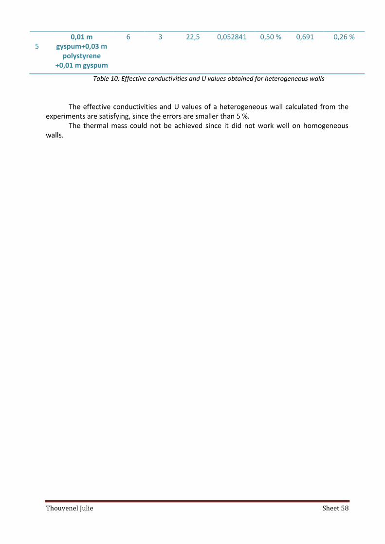
Thouvenel Julie Sheet 58
5 5
0,01 m gyspum+0,03 m
polystyrene +0,01 m gyspum
6 3 22,5 0,052841 0,50 % 0,691 0,26 %
Table 10: Effective conductivities and U values obtained for heterogeneous walls
The effective conductivities and U values of a heterogeneous wall calculated from the
experiments are satisfying, since the errors are smaller than 5 %. The thermal mass could not be achieved since it did not work well on homogeneous
walls.
Thouvenel Julie Sheet 59
Conclusion
Determining the U value of a building envelope is feasible using an IR camera. If the external heat transfer coefficient is determined, the thermal images allow determining the conductivity of a homogeneous wall and the effective conductivity of a heterogeneous wall with high accuracy (error less than 10 %).
When the heat transfer coefficient is determined with the camera, the method that
works the most is the method considering the central point temperature given by the camera, and using the entire area heated in the calculations. Then the central point can be representative of the area heated.
Taking the central point temperature to get the best result can be logical, since the formulas used to calculate all the values are taken for heat conduction in a one-dimensional wall. It is in the central point that this approximation is the most accurate. The experiment is normally in three dimensions and the heat flow is not only in the x direction but also in the other directions.
However the method proposed in this paper should be a quick method to determine the material’s properties, approaching the real values but it is not supposed to give the exact results. Then in this purpose the one-dimensional approximation could work, taking the temperature at the center of the wall to deduce reliable results.
Taking a mean value over a specific area seen by the camera works quite well also, giving results of less than 10% error, so the one-dimensional approximation is quite close and could be taken for a small area around the central point.
The thickness does not interfere a lot in the results. For one or three layers of material the conductivity found with the method is really close to the real one. This also confirms that the one-dimensional approximation is not so far from the real situation and can be applied in this case.
More accuracy is obtained with only one layer, which can be caused by the contact between the different layers. No contact resistance has been calculated in the case of several layers put together, which can lead to small errors compared to one layer. However the result stays accurate enough to be an approximate method for a first guess of the conductivity of the material. The thermal mass can then be approximated using the tool Solver, but the user must have a good guess of the value before running the solver. For this reason this application is limited, but the method could be developed more, since the thermal mass of a building is an interesting parameter to determine. For a heterogeneous material the U value can be also well defined, with really small errors if the heat transfer is determined.
The application of the method proposed is less relevant when the external heat transfer coefficient is not known.
The idea for determining the materials’ characteristics for a heterogeneous building wall was to make several nodes between the layers, similar to the surface node that was studied previously.
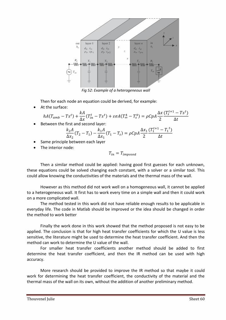
Thouvenel Julie Sheet 60
Fig 52: Example of a heterogeneous wall
Then for each node an equation could be derived, for example:
At the surface:
Between the first and second layer:
Same principle between each layer
The interior node:
Then a similar method could be applied: having good first guesses for each unknown,
these equations could be solved changing each constant, with a solver or a similar tool. This could allow knowing the conductivities of the materials and the thermal mass of the wall.
However as this method did not work well on a homogeneous wall, it cannot be applied
to a heterogeneous wall. It first has to work every time on a simple wall and then it could work on a more complicated wall.
The method tested in this work did not have reliable enough results to be applicable in everyday life. The code in Matlab should be improved or the idea should be changed in order the method to work better Finally the work done in this work showed that the method proposed is not easy to be applied. The conclusion is that for high heat transfer coefficients for which the U value is less sensitive, the literature might be used to determine the heat transfer coefficient. And then the method can work to determine the U value of the wall. For smaller heat transfer coefficients another method should be added to first determine the heat transfer coefficient, and then the IR method can be used with high accuracy. More research should be provided to improve the IR method so that maybe it could work for determining the heat transfer coefficient, the conductivity of the material and the thermal mass of the wall on its own, without the addition of another preliminary method.
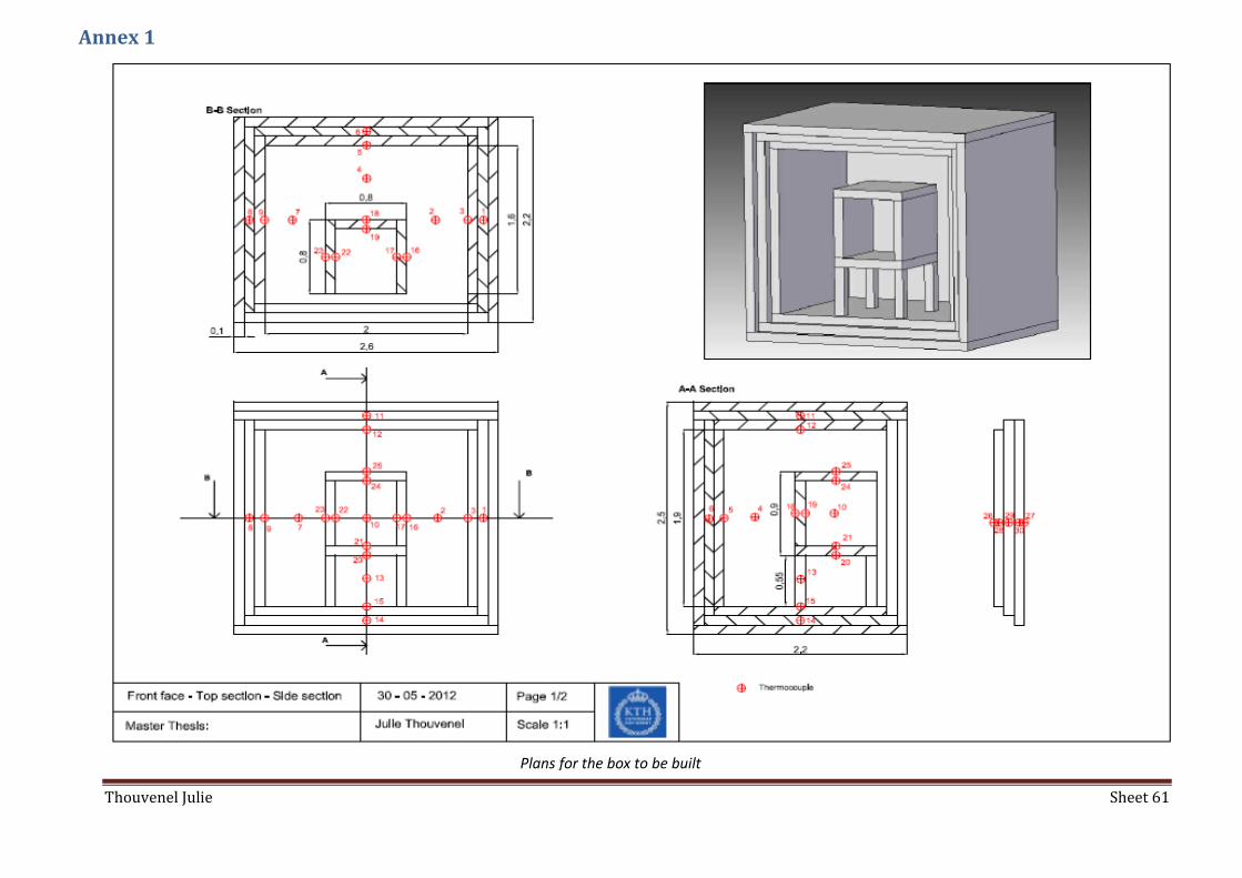
Thouvenel Julie Sheet 61
Annex A1
Plans for the box to be built
Annex 1

Thouvenel Julie Sheet 62
References [1] Organization for Standardization (ISO), ISO 9869: Thermal insulation! Building elements- In-situ measurement of thermal resistance and thermal transmittance, 1994 [2] C.A Balaras, A.A Argiriou, Infrared thermography for building diagnostics, 2002, Energy and Buildings 34, pp. 171-183 [3] Eva Barreira, Vasco P. de Freitas, Evaluation of building materials using infrared thermography, 2007, Construction and Building Materials 21, pp.218–224 [4] Paris A. Fokaides, Soteris A. Kalogirou, Application of infrared thermography for the determination of the overall heat transfer coefficient (U-Value) in building envelopes, 2011, Applied Energy 88, pp. 4358–4365 [5] Stefan Datcu,Laurent Ibos, et al., Improvement of building wall surface temperature measurements by infrared thermography, 2005, Infrared Physics & Technology 46, pp. 451–467 [6] L. Terry Clausing, Emissivity: Understanding the difference between apparent and actual infrared temperatures, 2005, Fluke corporation, Available from : http://support.fluke.com/educators/Download/Asset/2563251_6251_ENG_B_W.PDF [7] T. Kisilewicz, A. Wróbel, Quantitative infrared wall inspection, July 27-30, 2010, Cracow University of Technolog, 10th International Conference on Quantitative Infrared Thermography [8] Frank P. Incropera, David P. Dewitt, Introduction to heat transfer, 1996, John Wiley & Sons [9] Carosena Meola, Giovanni M. Carlomagno, Recent advances in the use of infrared thermography, 2004, Meas. Sci. Technol. 15, R27–R58, Available from : http://iopscience.iop.org/0957-0233/15/9/R01/pdf/0957-0233_15_9_R01.pdf [10] Yoav Peles, Transient Heat Conduction, The McGraw-Hill Companies, Inc, Available from : http://wwwme.nchu.edu.tw/Enter/html/lab/lab516/Heat%20Transfer/chapter_4.pdf [11] Dr. P.J. Schneider, Temperature response charts, 1963, John Wiley and Sons, Inc. [12] Sustainable energy authority, Thermal mass, Available from: http://www.sustainability.vic.gov.au/resources/documents/Thermal_mass.pdf, [31/05/12] [13] Chris Reardon, Thermal mass, 2010, Commonwealth of Australia, Available from: http://www.yourhome.gov.au/technical/pubs/fs49.pdf [14] Seog-Kwang Kim, Yong-Jin Kim, Determination of apparent thickness of graphite coating in flash method, 2008, Thermochimica Acta 468, pp.6–9

Thouvenel Julie Sheet 63
[15] Netzch, Laser Flash Analysis -LFA [16] Dr.-Ing. Wolfgang Hohenauer, Laser Flash Method to Determine Thermal Conductivity, Available from : http://www.phox.at/upload/Laser%20Flash%20Method%20to%20Determine%20Thermal%20Conductivity.pdf [17] User’s manual, ThermaCAM Researcher, December 21st, 2006, Flir Systems [18] W. J. Parker, R. J. Jenkins, et al., Flash Method of Determining Thermal Diffusivity, Heat Capacity, and Thermal Conductivity, American Institute of Physics, 1961, Journal of Applied Physics 32, 1679 [19] John Richard Thome, Numercial techniques for conduction, March 2010, EPFL, available from : http://ltcm.epfl.ch/files/content/sites/ltcm/files/shared/import/migration/COURSES/HeatAndMassTransfer/Num_conduction.pdf [20] Xavier Maldague, Application of infrared thermography in nondestructive evaluation, Université Laval, Available from: http://w3.gel.ulaval.ca/~maldagx/r_1123.pdf