Financial Stability Review (FSR) · The PDF format is downloadable from: ... [email protected] ......
168
Transcript of Financial Stability Review (FSR) · The PDF format is downloadable from: ... [email protected] ......


The preparation of the Financial Stability Review (FSR) is one of the avenues
through which Bank Indonesia achieves its mission “to safeguard the stability of the Indonesian
Rupiah by maintaining monetary and financial system stability for sustainable national
economic development”.
Publisher:
Bank Indonesia
Information and Orders:
This edition is published in September 2014 and is based on data and information available as of June 2014,unless stated otherwise.
Source: Bank Indonesia, unless stated otherwise.
The PDF format is downloadable from: http://www.bi.go.id
For inquiries, comments and feedback please contact:
Bank Indonesia
Macroprudential Policy Department (DKMP)
Jl.MH Thamrin No.2, Jakarta, Indonesia
Email: [email protected]
FSR is published biannually with the objectives:
To improve public insight in terms of understanding financial system stability.
To evaluate potential risks to financial system stability.
To analyze the developments of and issues within the financial system.
To offer policy recommendations to promote and maintain financial system stability.

Financial Stability Review( No.23, September 2014)
MACROPRUDENTIAL POLICY DEPARTMENT
ii
“Maintaining Financial Stabilityamid Economic Slowdown”

iii
Table of Contents ........... ................................................................................................................................................. iii
Glossary ............ ............................................................................................................................................................... vii
Foreword.......... ................................................................................................................................................................ ix
......................................................................................................................................................... 3 Chapter 1. Financial System Stability ................................................................................................................................ 9 1.1. Development of Risks on Global and Regional Financial Markets .................................................................. 9
........................................................................................... 12 1.3. Financial System Stability in Indonesia ........................................................................................................... 14 1.4. The Financial Cycle of Indonesia .................................................................................................................... 15 1.5. Sources of Financial Imbalances .................................................................................................................... 17 1.6. Sources of Vulnerability ................................................................................................................................. 24 Box 1.1. Financial Cycle of Indonesia ................................................................................................................... 32
........................................................................................ 36.......................................................... 38
Chapter 2. Financial Markets ........................................................................................................................................... 43 2.1. Financial Market Risks .................................................................................................................................... 43 2.2. The Financial Market as a Source of Non-Bank Financing ............................................................................. 55
.................................................................................... 59 Box 2.2. Shadow Banking in Indonesia ................................................................................................................. 63 Chapter 3. The Household and Corporate Sectors ........................................................................................................... 69 3.1. Household Sector Assessment ....................................................................................................................... 69 3.2. Corporate Sector Assessment ........................................................................................................................ 76
................................................................................. 85 ................................................................................. 86
............................................................................ 91 4.1. The Banking Sector ......................................................................................................................................... 91
......................................................................................................... 114 ........................................................................... 118
........................... 120
Chapter 5. Financial System Infrastructure ...................................................................................................................... 125 ....................................................................................................................... 126
................................................................................................... 127 ............................................................................................................................ 128
.................................................................................................. 130 .......................................................................................... 131
.............................................................................................................................................................. 133 .......................................................................................... 135
............................................................................................................... 145
Bibliography ..... ................................................................................................................................................................ 153
able ntent

iv
i t able a an Fi e
able1.1. . 101.2. .. 161.3. Stress/Crisis ........................................................ 171.4. Several Countries with the Strongest
............................ 28Box Table 1.1.1. Concordance Index of Financial Cycle Variables (Narrow Credit) ..................................... 33Box Table 1.1.2. Concordance Index of Financial Cycle Variables (Broad Credit) ..................................... 33
Business Cycle ................................................... 34
onset of Crisis/Stress ......................................... 34
2.1. 10-Year SBN Yield and Regional Yields ............. 482.2. .. 48
............. 512.4. Bank and Non-Bank Financing ......................... 552.5. .. 562.6. Volume of Bank Funding based on
........................... 57Box Table 2.1.1. Funding through the Capital Market
.................................... 60
......... 703.2. and Savings based on Monthly Income .............. 73
............................................ 733.4. .. 74
.................................... 793.6. by Sector ........................................................... 79
............ 823.8. Corporate Credit by Economic Sector .............. 82
Economic Sector ............................................... 83
Direct Investment by Economic Sector ............ 84Box Table
................ 87Box Table
................. 87
Box Table 3.2.3 Altman Z-score ................................... 88Box Table
Exchange Rates ................................................ 88
....................... 93 ............................... 93
........................ 94 ... 95
........................ 95 ............................... 96
.............. 98 ..................... 99
........................................ 101 ............. 101
4.11. Deposit Rates .................................................. 103 ......................... 104
the Banking Sector ........................................... 1054.14. SBN Holdings in the Banking Sector ................. 106
(in trillions of rupiah) ....................................... 1064.16. Breakdown of Income Accounts (in trillions of rupiah) ....................................... 1074.17. Breakdown of Cost Accounts (in trillions of rupiah) ....................................... 107
...................... 108 ............................... 110
........ 116 .......................... 117
Box Table 4.1.1. Granger Causality Test ....................... 118Box Table 4.1.2. Regression of MSME Credit Risk ............ 118
and Electronic Money ...................................... 127

v
a .......................... 11
............... 11 ......... 12
........................................ 131.5. External Debt ................................................... 131.6. Financial System Stability Index ....................... 14
in June 2014 ....................................................... 141.8. Financial Cycle of Indonesia ............................. 15
............................. 18 ........................... 18
...................... 19
............................ 19
.............................................. 201.14. ............ 20
................. 21 ..................... 23
1.17. Sources of Funds and Instruments of ..... 23
1.18. External Debt by Tenor ..................................... 231.19. External Debt by Economic Sector ................... 241.20. Fed Fund Survey: .................. 251.21. Growth in Emerging Market Countries ............ 251.22. CDS in Advanced Countries .............................. 261.23. CDS in Neighbouring Countries ........................ 261.24. CDS in Several Emerging Market Countries ...... 27
Emerging Market Countries ............................. 27
and SBN ............................................................ 281.27. Financial Account ............................................. 291.28. Current Account and Exchange Rate ............... 29
............................ 301.30. RI Counterpart Exports in 2013 ........................ 30
........................................... 311.32. Value of Bond Issuances ................................... 311.33. Growth of Deposits and Credit as well as
................................ 31Box Graph 1.1.1. A Common Cycle of the Financial Cycle (Narrow Credit) and Business Cycle ........ 33Box Graph 1.1.2. A Common Cycle of the Financial Cycle (Broad Credit) and Business Cycle .......... 33Box Graph 1.2.1.Macroeconomic Indicators of Indonesia during the 2008 Crisis and Current .. 36Box Graph 1.2.2 Credit Imbalances ............................. 37Box Graph 1.2.3 Deposit Imbalances ........................... 37
2.1. Non-Resident Flows: Shares, SBN & SBI .......... 442.2. .. 44
..................... 44....................... 45
...... 452.6. Foreign Exchange Interbank Money Market .... 45
.... 45 ...... 46
Behaviour ......................................................... 46 ........................... 46 ............................ 46
......... 47 ............................... 47
.... 47 ... 47
2.16. Foreign Net Flow to SBN and IDMA Index ....... 482.17. SBN Holdings .................................................... 40
..................................... 492.19. Rebased SBN Yield by Tenor ............................. 49
.................. 502.21. Rebased Corporate Bond Yield by Tenor .......... 502.22. Corporate Bond Yield Curve ............................. 50
.................... 502.24. Foreign Net Flow and Holdings of Corporate Bonds.. 50
............... 51 ...................... 51
2.27. Flow to Shares and JCI ...................................... 51 ............................... 52
............................. 52 ...................... 52
................. 522.32. Growth of Mutual Funds (yoy) ........................ 53
................................ 532.34. NAV trend of Mutual Funds by Type ............... 532.35. NAV of Mutual Funds by Type ......................... 54
............... 542.37. Nominal Value of Bonds ................................... 552.38. Capital Market Financing ................................. 56
..... 59 ..... 59
....... 60 ....... 60
2013-Semester I 2014 ........................................ 61
2013-Semester I 2014 ...................................... 61 ..................................... 61
................................... 61

vi
aBox Graph 2.1.9. JCI, Yield and the Rupiah in 2014 ..... 62Box Graph 2.1.10. Actual and Forecasted Indicators ... 62Box Graph 2.2.1. Exposure of Non-Bank Financial
Intermediaries .................................................. 64Box Graph 2.2.2. Growth of Non-Bank Financial
Intermediaries .................................................. 64
3.1. .. 70 .................................................... 70
3.3. Retail Sales Growth .......................................... 713.4. .. 723.5. .. 72
............... 73 ......................... 74
......... 75
(per June) ......................................................... 75 .......... 76
... 76 .... 76
3.13. Total Number of Companies ............................ 76 .... 77
................................. 77
..................................................... 783.17. .. 79
Z-score .............................................................. 80 ... 80
................................ 80 .... 81 .... 81
................................. 82Box Graph 3.1.1. Non-Regional Commercial Bank Credit
.............................. 85Box Graph 3.2.1 . 87
.................................................. 924.2. . 92
.... 924.4. Deposit Growth (yoy) ....................................... 944.5. .... 94
......................... 94 ..................... 96
4.8. Increases in Interest Rates ............................... 964.9. Credit Growth .................................................. 974.10. Credit Growth by Currency .............................. 97
............................. 974.12. Credit Growth by Economic Sector .................. 98
.............................. 99
4.14. Annual MSME Credit Growth by Economic Sector 99 ............... 100 ................ 100
......................... 100
............................................................ 101 ............ 102
Semester I-2014 ............................................... 104 ......................................................... 105
............ 108 .................... 108
........................................ 109 ......... 109
................................. 110 .................... 110
4.28. ...................... 111
................................................. 111 ................. 112
Higher Interest Rates ........................................ 112 .................. 112
......................................... 113 ....................... 113
.............................................. 1134.36. Finance Company Financing by Business Sector . 114
....................... 114 ..................... 114
4.39. Sources of Funds .............................................. 115 ...... 116
in Semester I-2014 ........................................... 1164.42. Share of Industry Assets by Business Sector (per December 2013) ....................................... 1164.43. Insurance Industry Assets and Investments ...... 1164.44. . 1164.45. Insurance Industry Growth and Density........... 117Box Graph 4.1.1. Credit Risk and Economic Growth .... 119
5.1. .. 128 ......................... 129
.......................... 129 ....................... 129
vii
GlossaryAFS: Available for SaleUS: United StatesAPMK: Card-based payment instrumentsASEAN: AssociationofSoutheastAsianNationsATM: AutomaticTellerMachineATMR: Risk-weightedassetsBCBS: BaselCommitteeonBankingSupervisionBIS: BankforInternationalSettlementsBI-RTGS: BankIndonesia–RealTimeGross
Settlement(BI-RTGS)systemBI-SSSS: BankIndonesiaScriplessSecurities
SettlementSystemBOPO: Efficiencyratioofoperatingcoststo
operatingincomeBPD: Regional bankBPR: Rural Bankbps: basis pointBUKU: Classificationofcommercialbanksbasedon
businessactivityBUS: Islamic bankCAR: CapitalAdequacyRatioCCB: CountercyclicalcounterbufferCDS: Credit Default SwapCPO: Crude palm oilDER: DebttoequityratioDTI: DebttoincomeratioDPK: DepositsD-SIB: Domestic–SystemicallyImportantBankDP: DownpaymentDRC: Disaster Recovery CentreDSR: DebtServiceRatioEM: EmergingMarketFDI: Foreign Direct InvestmentFKSSK: FinancialSystemStabilityCoordination
ForumFSAP: Financial Sector Assessment ProgramFSB: Financial Stability BoardFSI: Financial Stability IndexG20: TheGroupofTwentyGDP: GrossDomesticProductIDMA: InterdealerMarketAssociationIHK: ConsumerPriceIndex(CPI)IHSG: IDX Composite IndexIKK: ConsumerConfidenceIndex(CCI):IKNB: Non-bankfinancialinstitutionIMF: InternationalMonetaryFundISIK: FinancialInstitutionStabilityIndexISPK: FinancialMarketStabilityIndexISSK: Indonesia Financial Stability Index
KI: Investment CreditKIK: Consumer LoansKMK: Working Capital CreditKPMM: MinimumStatutoryCapitalRequirementKPR: MortgageloanLCR: LiquidityCoverageRatioLDR: LoantodepositratioLKD: Digital Financial ServicesLTV: Loan to valueLPS: TheDepositInsuranceCorporationL/R: Profit/lossMinerba: MineralandCoalMiningNAB: NetAssetValueNFA: NetForeignAssetsNFL: NetForeignLiabilitiesNII: NetInterestIncomeNIM: NetInterestMarginNPF: Non-performingfinancingNPI: Indonesia Balance of PaymentsNPL: Non-performingloansOJK: TheFinancialServicesAuthority(OJK)OTC: OverthecounterPUAB: TheInterbankMoneyMarketPD: Probability of DefaultPDB: GrossDomesticProductPDN: NetOpenPositionPMK: MinisterofFinanceRegulationPLN: External debtPP: Finance CompanyRBB: Bank Business PlanROA: Return on assetsROE: Return on equitySBDK: Prime lending rateSBI: BankIndonesiaCertificateSBN: TradeableGovernmentSecuritiesSBT: NetweightedbalanceSKDU: Business SurveySKNBI: BankIndonesia-NationalClearingSystemSUN: GovernmentbondTOR: TurnoverratioTPT: TextilesandtextileproductsUMKM: Micro,SmallandMediumEnterprises
(MSMEs)

viii
This page is intentionally left blank
ix
rd
2014. The Financial Stability Review represents one form of transparency and accountability to the public in terms of
an expansionary period as well as provide space to absorb risk during an economic downturn.
the forms of spiralling private external debt, uncertainty surrounding the economic recovery in advanced countries as
amongst others.
In closing, this 23rd
of the Financial Stability Review.
Foreword
Jakarta, September 2014
Martowardo o

This page is intentionally left blank

1
ec ve S ary

2

3
ec ve S ary

4


7
Chapter 1. Financial System Stability
Financial System Stability
Chapter 1

8
Chapter 1. Financial System Stability

9
Chapter 1. Financial System Stability
1.1 DEVELOPMENT OF RISKS ON GLOBAL AND
REGIONAL FINANCIAL MARKETS
Financial System StabilityChapter1

Chapter 1. Financial System Stability
Advanced Countries
United States 1.80 (16.44) (41.98) (43.65) 22.04 6.05 - -
UK 9.29 (11.65) (61.51) (31.85) 8.50 (0.08) (11.07) (3.53)
Japan -33.65 (23.62) (53.28) (7.11) 10.86 45.86 2.21 (3.63)
Germany -27.95 (35.46) (38.05) (19.74) 23.54 38.46 (4.97) 0.83
East Asia
China 13.30 (11.47) (44.32) (3.54) 3.49 (3.20) 1.07 2.32
Hong Kong -0.10 (12.63) - - 11.48 (0.50) (0.08) (0.06)
Indonesia 15.17 (2.83) (22.37) (32.15) 1.24 13.02 18.70 (2.74)
South Korea -6.72 (11.79) (50.84) (19.38) 7.45 (0.03) (11.40) (4.14)
Malaysia 12.58 (2.02) (28.45) (22.48) 6.16 0.84 1.60 (2.53)
the Philippines - - (30.91) (23.03) 5.86 16.78 1.21 (1.67)
Singapore -1.20 (9.68) - - 3.34 2.79 (1.68) (1.66)
Thailand 2.20 (2.31) (14.30) (13.84) 2.33 5.67 4.47 (1.14)
Source: Bloomberg
(%)
(%)
Exchange RateStock IndexYield of 10-yearGovernment
Bonds (%)
5-year CDS (%)
y-o-y y-t-d y-o-y y-t-d y-o-y y-t-d y-o-y y-t-d

Chapter 1. Financial System Stability
45
Dow Jones
40
35
30
25
20
15
10
5
0
Jan
-13
Feb
-13
Mar
-13
Ap
r-13
May
-13
Jun
-13
Jul-
13
Au
g-13
Sep
-13
Oct
-13
No
v-13
Dec
-13
Jan
-14
Feb
-14
Mar
-14
Ap
r-14
May
-14
Jun
-14
MSCI AsiaMSCI EuroMSCI World
160
150
140
130
120
110
100
90
80Jan-10 Jul-10 Jul-11Jan-11 Jul-12Jan-12 Jul-13Jan-13 Jul-14Jan-14
80
90
100
110
120
130Index
Composite Stock Index Performance(Rebased 1/1/2010=100)
EM Asia
World
G7
Asia P
Index
Chapter 1. Financial System Stability
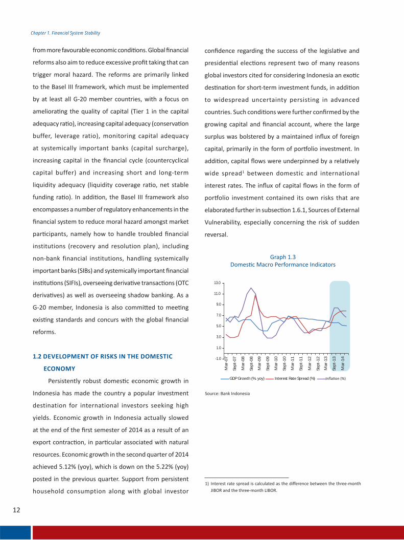
1.2 DEVELOPMENT OF RISKS IN THE DOMESTIC
ECONOMY
13.0
11.0
9.0
7.0
5.0
3.0
1.0
GDP Growth (%. yoy) Interest Rate Spread (%)
-1.0
Mar
-07
Sep
t-07
Mar
-08
Sep
t-08
Mar
-09
Sep
t-09
Mar
-10
Sep
t-10
Mar
-11
Sep
t-11
Mar
-12
Sep
t-12
Mar
-13
Mar
-14
Sep
t-13

Chapter 1. Financial System Stability
20.0M
ar-0
7
Sep
-07
Mar
-08
Sep
-08
Mar
-09
Sep
-09
Mar
-10
Sep
-10
Mar
-11
Sep
-11
Mar
-12
Sep
-12
Mar
-13
Mar
-14
Sep
-13
15.0
10.0
5.0
-5.0
0.0
-10.0
Current Account (billions of US$)
-15.0
Capital and Financial Account (billions of US$)
Overall Balance (billions of US$)
300.0
millions US$
Private – Non bank
250.0
200.0
150.0
100.0
50.0
0.02009 2010 2011 2012 2013 June 2014
Private – Bank Government andCentral Bank

Chapter 1. Financial System Stability
1.3. FINANCIAL SYSTEM STABILITY IN INDONESIA
nd
nd
3,0
2,5
1,5
0,5
2,0
1,0
2002
M01
2002
M05
2002
M09
2003
M01
2003
M05
2003
M09
2004
M01
2004
M05
2004
M09
2005
M01
2005
M05
2005
M09
2006
M01
2006
M05
2006
M09
2007
M01
2007
M05
2007
M09
2008
M01
2008
M05
2008
M09
2009
M01
2009
M05
2009
M09
2010
M01
2010
M05
2010
M09
2011
M01
2011
M05
2011
M09
2012
M01
2012
M05
2012
M09
2013
M01
2013
M05
2013
M09
2014
M01
2014
M05
1.2%
10.5%
2.6%6.4%
0.1%
0.5%
Banks
78.6%
Rural Banks
Insurers
Pension Funds
Finance Companies
Guarantors
Pawnbrokers
Chapter 1. Financial System Stability
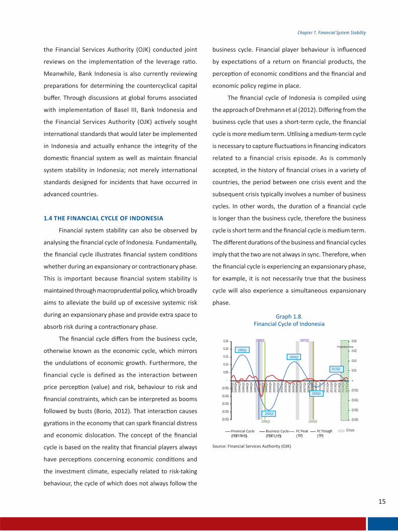
1.4 THE FINANCIAL CYCLE OF INDONESIA
0.25 0.02
0.02
0.01
0.01
(0.01)
(0.01)
(0.02)
(0.02)
2007Q2
0.20
0.15
0.10
0.05
-
(0.05)
19
92
Q1
19
93
Q4
19
94
Q3
19
95
Q2
19
96
Q1
19
96
Q4
19
97
Q3
19
98
Q2
19
99
Q1
19
99
Q4
20
00
Q3
20
01
Q2
20
02
Q1
20
02
Q4
20
03
Q3
20
04
Q2
20
05
Q1
20
05
Q4
20
06
Q3
20
07
Q2
20
08
Q1
20
08
Q4
20
09
Q3
20
10
Q2
20
11
Q1
20
11
Q4
20
12
Q3
20
13
Q2
20
14
Q1
20
14
Q4
20
15
Q3
(0.10)
(0.15)
(0.20)
(0.25)
1995Q1
2000Q2
2009Q4
2013Q3
2005Q2
1998Q2
1999Q2
(FBF/RHS)
2009Q3
(FBF/LHS) (TP)rough
(TP)
Chapter 1. Financial System Stability
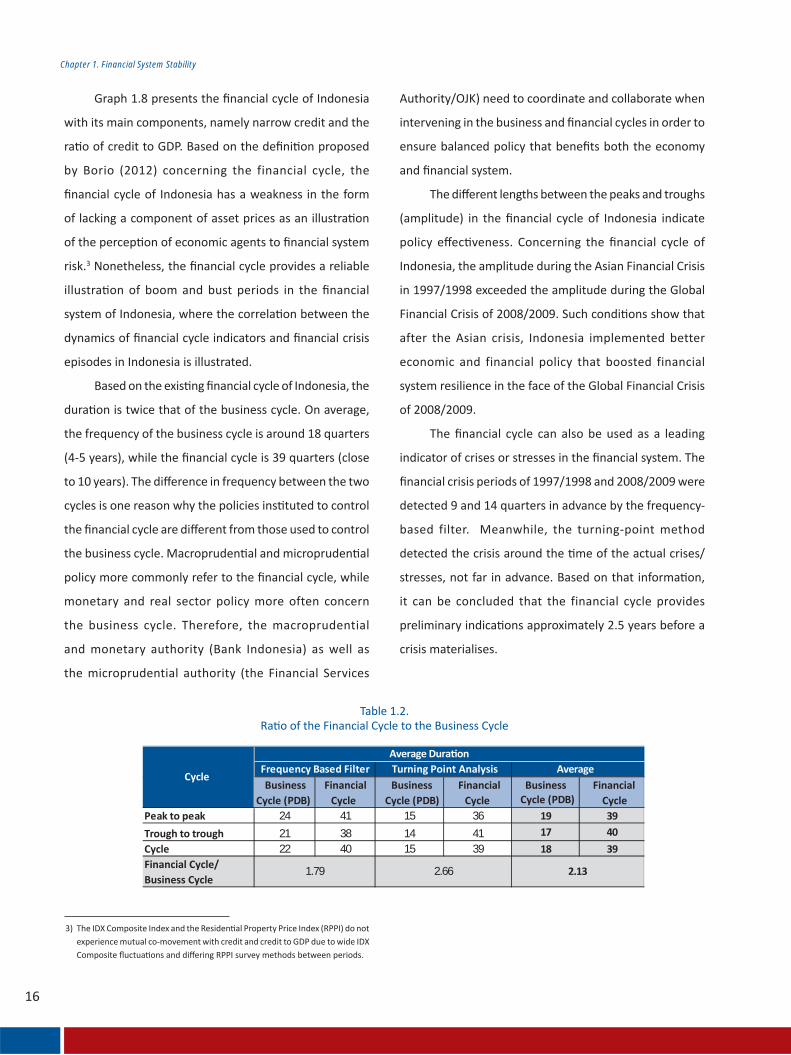
Peak to peak 24 41 15 36 19 39
Trough to trough 21 38 14 41 17 40
Cycle 22 40 15 39 18 39Financial Cycle/Business Cycle
BusinessCycle (PDB)
FinancialCycle
1.79 2.66 2.13
Cycle
Average Dura onFrequency Based Filter Turning Point Analysis AverageBusiness
Cycle (PDB)Financial
CycleBusiness
Cycle (PDB)Financial
Cycle

Chapter 1. Financial System Stability
7
8
Frequency based lter
Turning point
analysis
1997Q3 -10 3Economic crisis and
2005Q3 -1 - Mini economic crisis2008Q4 -14 -6 Economic crisis
Crisis Descrip on
Peak (Quarterly)
1.5 SOURCES OF FINANCIAL IMBALANCES
1.5.1 Banking Procyclicality

Chapter 1. Financial System Stability
40.0 8.0
7.0
5.0
4.0
3.0
2.0
1.0
6.0
35.0
30.0
25.0
20.0
15.0
10.0
5.0
0.0
Sep-
01M
ar-0
2Se
p-02
Credit Growth (%. yoy) GDP Growth (%. RHS)
Mar
-03
Sep-
03M
ar-0
4Se
p-04
Mar
-05
Sep-
05M
ar-0
6Se
p-06
Mar
-07
Sep-
07M
ar-0
8Se
p-08
Mar
-09
Sep-
09M
ar-1
0Se
p-10
Mar
-11
Sep-
11M
ar-1
2Se
p-12
Mar
-13
Sep-
13M
ar-1
4Se
p-14
1.5.2 Rising Property Prices
9
40.0 3.0
2.5
1.5
1.0
0.5
0.0
-0.5
-1.0
-1.5
-2.0
2.035.0
30.0
25.0
20.0
15.0
10.0
Sep-
01M
ar-0
2Se
p-02
Credit/GDP Gap (%. RHS) Credit/GDP (%) Trend
Mar
-03
Sep-
03M
ar-0
4Se
p-04
Mar
-05
Sep-
05M
ar-0
6Se
p-06
Mar
-07
Sep-
07M
ar-0
8Se
p-08
Mar
-09
Sep-
09M
ar-1
0Se
p-10
Mar
-11
Sep-
11M
ar-1
2Se
p-12
Mar
-13
Sep-
13M
ar-1
4Se
p-14
40%
Overheated Overheated
Overheated
Overheated
35
30
25
20
15
Sep-
01M
ar-0
2Se
p-02
Mar
-03
Sep-
03M
ar-0
4Se
p-04
Mar
-05
Sep-
05M
ar-0
6Se
p-06
Mar
-07
Sep-
07M
ar-0
8Se
p-08
Mar
-09
Sep-
09M
ar-1
0Se
p-10
Mar
-11
Sep-
11M
ar-1
2Se
p-12
Mar
-13
Sep-
13M
ar-1
4Se
p-14
Credit/GDP (%) Trend

Chapter 1. Financial System Stability
180.00
170.00
160.00
150.00
140.00
130.00
120.00
110.00
100.00
2007 2008 2009 2010 2011 2012 2013 2014
240.00
220.00
200.00
180.00
160.00
140.00
120.00
2007 2008 2009 2010 2011 2012 2013 2014
Bandung Jabotabek-Banten
220.00
200.00
180.00
160.00
140.00
120.00
100.00
2007 2008 2009 2010 2011 2012 2013 2014
Palembang Bandar Lampung
240.00
220.00
200.00
180.00
160.00
140.00
120.00
100.00
2007 2008 2009 2010 2011 2012 2013 2014
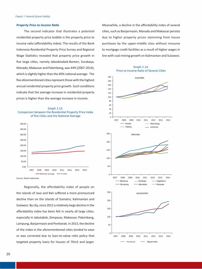
Chapter 1. Financial System Stability
0.00
50.00
100.00
150.00
200.00
250.00
300.00
350.00
400.00
2007 2008 2009 2010 2011 2012 2013 2014
200
180
SUMATERA
Medan
Padang
Palembang
Lampung
160
140
120
100
80
60
40
20
2007 2008 2009 2010 2011 2012 2013 2014
0
250
200
150
100
50
02007 2008 2009 2010 2011 2012 2013 2014
JAWA-BALI
Bandung
Semarang
Surabaya
Jabotabek
Yogyakarta
Denpasar
250
200
150
100
50
02007 2008 2009 2010 2011 2012 2013 2014
KALIMANTAN
Banjarmasin

Chapter 1. Financial System Stability
180
160
140
120
100
80
60
40
20
02007 2008 2009 2010 2011 2012 2013 2014
Menado Makasar
2007 2008 2009 2010 2011 2012 2013 2014
1.20
1.10
1.00
0.90
0.80
0.70
0.60
Tw I Tw II Tw IIITw IV Tw I Tw II Tw IIITw IV Tw I Tw II Tw IIITw IV Tw I Tw II Tw IIITw IV Tw I Tw II Tw IIITw IV Tw I Tw II Tw IIITw IV Tw I Tw II Tw IIITw IV Tw I Tw II
Jabodetabek
Chapter 1. Financial System Stability
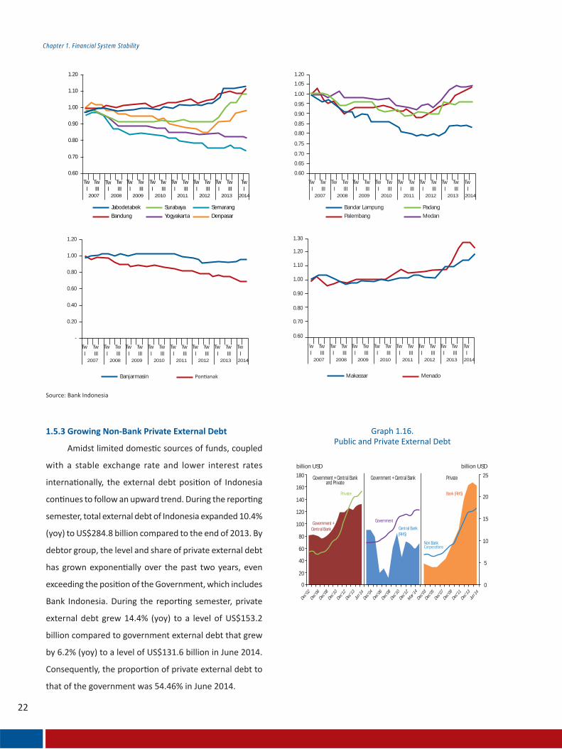
1.5.3 Growing Non-Bank Private External Debt
180
billion USD billion USD
25
20
15
10
5
0
Government + Central Bankand Private
Government + Central Bank
Private
Private
160
140
120
100
80
60
40
20
0
Government + Central Bank
Government
Central Bank (RHS)
Non Bank
Bank (RHS)
Dec’02
Dec’06
Dec’08
Dec’10
Dec’12
Dec’13
Jun’14
Dec’04
Dec’06
Dec’08
Dec’10
Dec’12
Mar
’14
Dec’03
Dec’05
Dec’07
Dec’09
Dec’11
Dec’13
Jun’14
2007
Jabodetabek
Bandung
Tw I
Tw III
2008
Tw I
Tw III
2009
Tw I
Tw III
2010
Tw I
Tw III
2011
Tw I
Tw III
2012
Tw I
Tw III
Tw I
Tw III
Tw I
1.20
1.10
1.00
0.90
0.80
0.70
0.60
2013 2014
Surabaya
Yogyakarta
Semarang
Denpasar
2007
Bandar Lampung
Palembang
Tw I
Tw III
2008
Tw I
Tw III
2009
Tw I
Tw III
2010
Tw I
Tw III
2011
Tw I
Tw III
2012
Tw I
Tw III
Tw I
Tw III
Tw I
1.20
1.05
1.00
0.95
0.85
0.90
0.80
0.70
0.75
0.60
0.65
2013 2014
Padang
Medan
2007
Banjarmasin
Tw I
Tw III
2008
Tw I
Tw III
2009
Tw I
Tw III
2010
Tw I
Tw III
2011
Tw I
Tw III
2012
Tw I
Tw III
Tw I
Tw III
Tw I
1.20
1.00
0.80
0.60
0.40
0.20
-
2013 2014
2007
Makassar Menado
Tw I
Tw III
2008
Tw I
Tw III
2009
Tw I
Tw III
2010
Tw I
Tw III
2011
Tw I
Tw III
2012
Tw I
Tw III
Tw I
Tw III
Tw I
1.30
1.20
1.10
1.00
0.90
0.80
0.70
0.60
2013 2014

Chapter 1. Financial System Stability
Government and Central Bank
100%
90%
80%
70%
60%
50%
40%
30%
20%
10%
0%
Dec
09
Dec
10
Dec
11
Dec
12
Dec
13
Jan
14
Feb1
4
Mar
14
Apr
14
May
14
Jun
14
Stocks16%
Bonds10%
ExternalDebt29%
Credit45%
LOANAGREEMENT
73.4%
BONDS19.9%
OTHERS0.4%
PAYABLES6.4%
Short Term20%
Long Term80%
24
Chapter 1. Financial System Stability
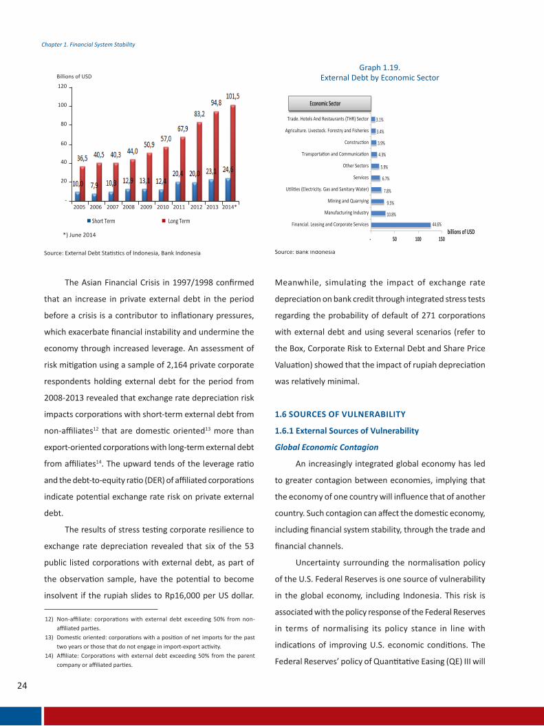
Source: External Debt Statistics of Indonesia, Bank Indonesia
*) June 2014
Source: Bank Indonesia
Graph 1.19.External Debt by Economic Sector
The Asian Financial Crisis in 1997/1998 confirmed
that an increase in private external debt in the period
before a crisis is a contributor to inflationary pressures,
which exacerbate financial instability and undermine the
economy through increased leverage. An assessment of
risk mitigation using a sample of 2,164 private corporate
respondents holding external debt for the period from
2008-2013 revealed that exchange rate depreciation risk
impacts corporations with short-term external debt from
non-affiliates12 that are domestic oriented13 more than
export-oriented corporations with long-term external debt
from affiliates14. The upward tends of the leverage ratio
and the debt-to-equity ratio (DER) of affiliated corporations
indicate potential exchange rate risk on private external
debt.
The results of stress testing corporate resilience to
exchange rate depreciation revealed that six of the 53
public listed corporations with external debt, as part of
the observation sample, have the potential to become
insolvent if the rupiah slides to Rp16,000 per US dollar.
12) Non-affiliate: corporations with external debt exceeding 50% from non-affiliated parties.
13) Domestic oriented: corporations with a position of net imports for the past two years or those that do not engage in import-export activity.
14) Affiliate: Corporations with external debt exceeding 50% from the parent company or affiliated parties.
Meanwhile, simulating the impact of exchange rate
depreciation on bank credit through integrated stress tests
regarding the probability of default of 271 corporations
with external debt and using several scenarios (refer to
the Box, Corporate Risk to External Debt and Share Price
Valuation) showed that the impact of rupiah depreciation
was relatively minimal.
1.6 SOURCES OF VULNERABILITY
1.6.1 External Sources of Vulnerability
Global Economic Contagion
An increasingly integrated global economy has led
to greater contagion between economies, implying that
the economy of one country will influence that of another
country. Such contagion can affect the domestic economy,
including financial system stability, through the trade and
financial channels.
Uncertainty surrounding the normalisation policy
of the U.S. Federal Reserves is one source of vulnerability
in the global economy, including Indonesia. This risk is
associated with the policy response of the Federal Reserves
in terms of normalising its policy stance in line with
indications of improving U.S. economic conditions. The
Federal Reserves’ policy of Quantitative Easing (QE) III will
120
Billions of USD
100
80
60
40
20
2005 2006 2007 2008 2009 2010 2011 2012 2013 2014*-
Short Term Long Term
- 50 100 150
44.6%
10.8%
9.5%
7.8%
6.7%
5.9%
4.3%
3.9%
3.4%
3.1%
billions of USD
Economic Sector
Trade. Hotels And Restaurants (THR) Sector
Agriculture. Livestock. Forestry and Fisheries
Construction
Transportation and Communication
Other Sectors
Services
Utilities (Electricity. Gas and Sanitary Water)
Mining and Quarrying
Manufacturing Industry
Financial. Leasing and Corporate Services
25
Chapter 1. Financial System Stability
14.0
12.0
10.0
8.0
6.0
4.0
2.0
-
INDI IND0 CHN KOR TUR
Q1 Q2
2010
Q3 Q4 Q1 Q2
2011
Q3 Q4 Q1 Q2
2012
Q3 Q4 Q1 Q2
2013
Q3 Q4 Q1 Q2
2014
Q3 Q4
2014 2015 2016
PercentAppropriate pace of policy firming
Target federal funds rate at year-end6
5
4
3
2
1
0
Longer Run
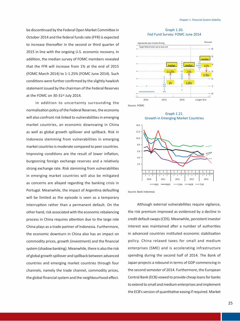
be discontinued by the Federal Open Market Committee in
October 2014 and the federal funds rate (FFR) is expected
to increase thereafter in the second or third quarter of
2015 in line with the ongoing U.S. economic recovery. In
addition, the median survey of FOMC members revealed
that the FFR will increase from 1% at the end of 2015
(FOMC March 2014) to 1-1.25% (FOMC June 2014). Such
conditions were further confirmed by the slightly hawkish
statement issued by the chairman of the Federal Reserves
at the FOMC on 30-31st July 2014.
In addition to uncertainty surrounding the
normalisation policy of the Federal Reserves, the economy
will also confront risk linked to vulnerabilities in emerging
market countries, an economic downswing in China
as well as global growth spillover and spillback. Risk in
Indonesia stemming from vulnerabilities in emerging
market countries is moderate compared to peer countries.
Improving conditions are the result of lower inflation,
burgeoning foreign exchange reserves and a relatively
strong exchange rate. Risk stemming from vulnerabilities
in emerging market countries will also be mitigated
as concerns are allayed regarding the banking crisis in
Portugal. Meanwhile, the impact of Argentina defaulting
will be limited as the episode is seen as a temporary
interruption rather than a permanent default. On the
other hand, risk associated with the economic rebalancing
process in China requires attention due to the large role
China plays as a trade partner of Indonesia. Furthermore,
the economic downturn in China also has an impact on
commodity prices, growth (investment) and the financial
system (shadow banking). Meanwhile, there is also the risk
of global growth spillover and spillback between advanced
countries and emerging market countries through four
channels, namely the trade channel, commodity prices,
the global financial system and the neighbourhood effect.
Although external vulnerabilities require vigilance,
the risk premium improved as evidenced by a decline in
credit default swaps (CDS). Meanwhile, persistent investor
interest was maintained after a number of authorities
in advanced countries instituted economic stabilisation
policy. China relaxed taxes for small and medium
enterprises (SME) and is accelerating infrastructure
spending during the second half of 2014. The Bank of
Japan projects a rebound in terms of GDP commencing in
the second semester of 2014. Furthermore, the European
Central Bank (ECB) vowed to provide cheap loans for banks
to extend to small and medium enterprises and implement
the ECB’s version of quantitative easing if required. Market
Source: FOMC
Graph 1.20.Fed Fund Survey: FOMC June 2014
Source: Bank Indonesia
Graph 1.21.Growth in Emerging Market Countries

Chapter 1. Financial System Stability
100
90
80
70
60
50
40
30
20
10
0
Jan-
13
Feb-
13
Mar
-13
Apr-
13
May
-13
Jun-
13
Feb-
14
Mar
-14
Apr-
14
May
-14
Jun-
14
Jul-1
3
Aug-
13
Sep-
13
Oct
-13
Nov
-13
Dec
-13
Jan-
14
USA UK GER JAP
i o n al
300
250
200
150
100
50
INDO
Jan-
13
Feb-
13
Mar
-13
Apr-
13
May
-13
Jun-
13
Feb-
14
Mar
-14
Apr-
14
May
-14
Jun-
14
Jul-1
3
Aug-
13
Sep-
13
Oct
-13
Nov
-13
Dec
-13
Jan-
14
THAI KOR PHI

Chapter 1. Financial System Stability
-150
-100
-50
0
50
100
150
200
250
20
05
Q1
20
05
Q2
20
05
Q3
20
05
Q4
20
06
Q1
20
06
Q2
20
06
Q3
20
06
Q4
20
07
Q1
20
07
Q2
20
07
Q3
20
07
Q4
20
08
Q1
20
08
Q2
20
08
Q3
20
08
Q4
20
09
Q1
20
09
Q2
20
09
Q3
20
09
Q4
20
10
Q1
20
10
Q2
20
10
Q3
20
10
Q4
20
11
Q1
20
11
Q2
20
11
Q3
20
11
Q4
20
12
Q1
20
12
Q2
20
12
Q3
20
12
Q4
20
13
Q1
20
13
Q2
20
13
Q3
20
13
Q4
Billion USD2
0000
8Q
1
20
08
QQ22
20
08
QQ33
20
08
Q4
20
12
Q4
20
13
Q1
20
13
Q2
20
13
Q3
GlobalFinancialCrisis
TaperingIssue
0
100
200
300
400
500
600
700
800
2005
Q1
2005
Q2
2005
Q3
2005
Q4
2006
Q1
2006
Q2
2006
Q3
2006
Q4
2007
Q1
2007
Q2
2007
Q3
2007
Q4
2008
Q1
2008
Q2
2008
Q3
2008
Q4
2009
Q1
2009
Q2
2009
Q3
2009
Q4
2010
Q1
2010
Q2
2010
Q3
2010
Q4
2011
Q1
2011
Q2
2011
Q3
2011
Q4
2012
Q1
2012
Q2
2012
Q3
2012
Q4
2013
Q1
2013
Q2
2013
Q3
2013
Q4
2014
Q1
2014
Q2
2014
Q3
BrazilSouth Africa
TurkeyIndonesia
MexicoSouth Korea
3 4 1 2
GlobalFinancialCrisis
TaperingIssue
2 3 4 1
TaperingIssue

Chapter 1. Financial System Stability
Period (T=Quarter) Country Sample
Prior to GlobalFinancial Crisis
T1 2007 –T2 2008 India, Hong Kong, South Korea Brazil, Russia, India,Hong Kong,South Africa,Turkey, Indonesia,Mexico andSouth Korea
Prior toTapering Issue
T1 2012 – T1 2013 India, South Korea, Turkey
T3 2013 – T4 2013 Indonesia, Hong Kong, Russia
50Trillions of Rp Shares
40
30
2010
2011
2012
2013
2014
20
10
0
-10
-20
2010
2011
2012
2013
2014
110
90
70
50
30
10
-10
Trillions of Rp

Chapter 1. Financial System Stability
Billions of USD
20
15
10
5
0
2010 2011 2012 2013-5
up to Q2 2014
Direct Investment
Other Investment
4,000
2,000
0
-2,000
-4,000
-6,000
-8,000
-10,000
-12,000
Current Account (million of US$) (LHS)
12,500
12,000
11,500
11,000
10,500
10,000
9,500
9,000
8,500
8,000
2010
Q1
2010
Q2
2010
Q3
2010
Q4
2011
Q1
2011
Q2
2011
Q3
2011
Q4
2012
Q1
2012
Q2
2012
Q3
2012
Q4
2013
Q1
2013
Q2
2014
Q1
2014
Q2
2013
Q3
2013
Q4
Exchange Rate (Rp/$) (RHS)

Chapter 1. Financial System Stability
1.6.2 Internal Sources of Vulnerability
130 rebased 1/1/2013
125
120
115
110
105
100
95
90
85
80
Indonesia
Jan-
13
Feb-
13
Mar
-13
Apr
-13
May
-13
Jun-
13
Feb-
14
Mar
-14
Apr
-14
May
-14
Jun-
14
Jul-1
3
Aug
-13
Sep-
13
Oct
-13
Nov
-13
Dec
-13
Jan-
14
Thailand South Korea the Philippines
Japan13.7%Others
44.4%
China15.0%
US9.0%
Europe8.8%
Singa-pore
Chapter 1. Financial System Stability
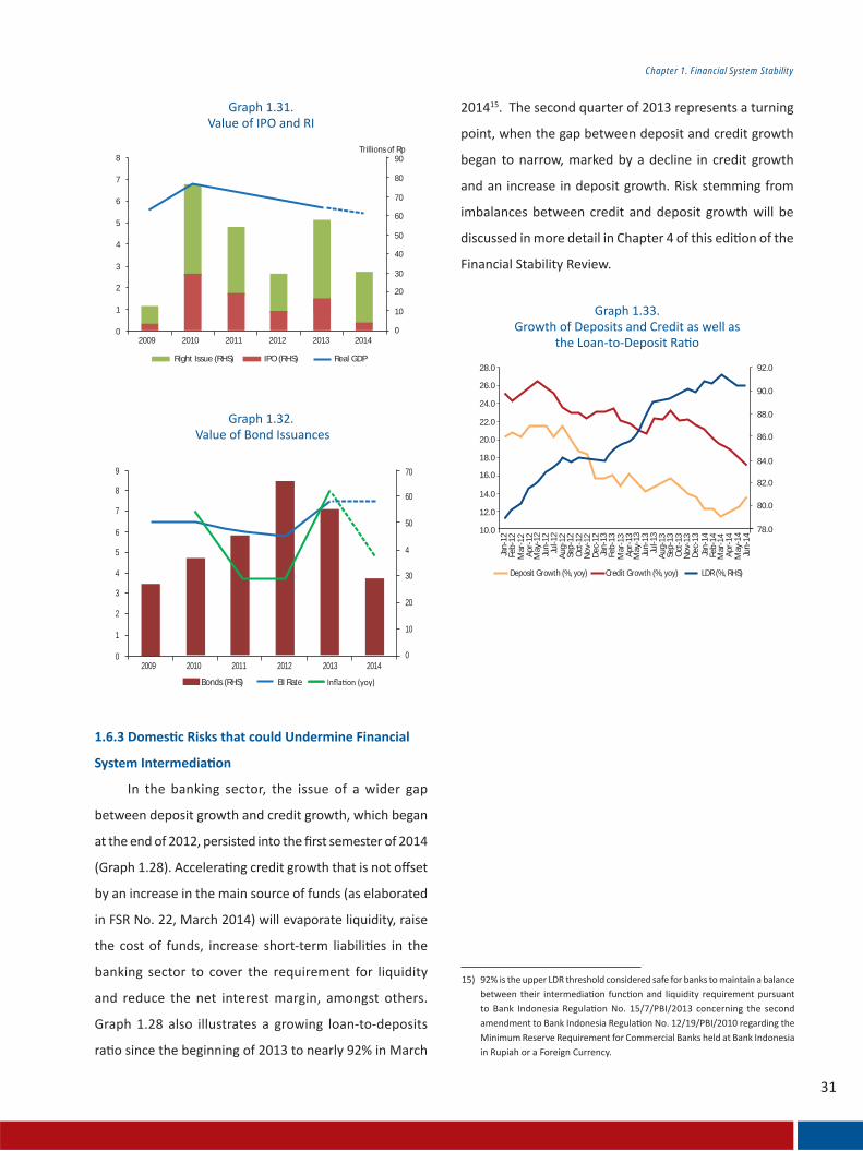
1.6.3 Domes c Risks that could Undermine Financial
System Intermedia on
8
7
6
5
4
3
2
1
02009
Right Issue (RHS) Real GDPIPO (RHS)
Trillions of Rp
2010 2011 2012 2013 2014
90
80
70
60
50
40
30
20
10
0
9
Bonds (RHS) BI Rate
8
7
6
5
4
3
2
1
02009 2010 2011 2012 2013 2014
70
60
50
4
30
20
10
0
28.0 92.0
90.0
88.0
86.0
84.0
82.0
80.0
78.0
26.0
24.0
22.0
20.0
18.0
16.0
14.0Ja
n-12
Feb-
12M
ar-1
2A
pr-1
2M
ay-1
2Ju
n-12
Jul-1
2A
ug-1
2Se
p-12
Oct
-12
Nov
-12
Dec
-12
Jan-
13Fe
b-13
Mar
-13
Apr
-13
May
-13
Jun-
13Ju
l-13
Aug
-13
Sep-
13O
ct-1
3N
ov-1
3D
ec-1
3Ja
n-14
Feb-
14M
ar-1
4A
pr-1
4M
ay-1
4Ju
n-14
12.0
10.0
Credit Growth (%, yoy)Deposit Growth (%, yoy) LDR (%, RHS)
Chapter 1. Financial System Stability
Box 1.1 Financial Cycle of Indonesia
= 1 [ + (1 )(1 )]=1
Chapter 1. Financial System Stability
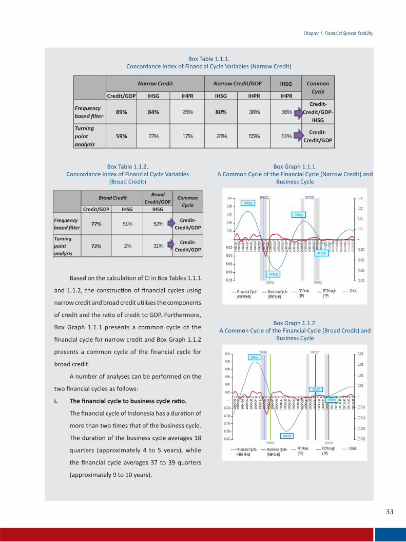
i. The nancial cycle to business cycle ra o.
IHSG
Credit/GDP IHSG IHPR IHSG IHPR IHPR
Frequency based lter
89% 84% 25% 80% 38% 36%Credit-
Credit/GDP-IHSG
Turning point analysis
59% 22% 17% 26% 55% 61%Credit-
Credit/GDP
Narrow Credit Narrow Credit/GDP Common Cycle
Broad Credit/GDP
Credit/GDP IHSG IHSG
Frequency based lter
77% 51% 52%Credit-
Credit/GDP
Turning point analysis
72% 2% 31%Credit-
Credit/GDP
Broad Credit Common Cycle
2007Q2
0.10
0.12
0.08
0.06
0.04
0.02
-
(0.02)
(0.04)
(0.06)
(0.08)
(0.10)
1996Q4
2002Q2
2007Q3
0.02
0.02
0.01
0.01
(0.01)
(0.01)
(0.02)
(0.02)
19
93
Q1
19
93
Q4
19
94
Q3
19
95
Q2
19
96
Q1
19
96
Q4
19
97
Q3
19
98
Q2
19
99
Q1
19
99
Q4
20
00
Q3
20
01
Q2
20
02
Q1
20
02
Q4
20
03
Q3
20
04
Q2
20
05
Q1
20
05
Q4
20
06
Q3
20
07
Q2
20
08
Q1
20
08
Q4
20
09
Q3
20
10
Q2
20
11
Q1
20
11
Q4
20
12
Q3
20
13
Q2
20
14
Q1
1998Q2
1999Q2 2009Q3
2009Q3
Financial Cycle(FBF/RHS)
Business Cycle(FBF/LHS)
FC Peak(TP)
FC Trough(TP)
Crisis
0.10 0.02
0.02
0.01
0.01
(0.01)
(0.01)
(0.02)
(0.02)
2007Q2
0.08
0.06
0.04
0.02
-
(0.02)
19
92
Q1
19
93
Q4
19
94
Q3
19
95
Q2
19
96
Q1
19
96
Q4
19
97
Q3
19
98
Q2
19
99
Q1
19
99
Q4
20
00
Q3
20
01
Q2
20
02
Q1
20
02
Q4
20
03
Q3
20
04
Q2
20
05
Q1
20
05
Q4
20
06
Q3
20
07
Q2
20
08
Q1
20
08
Q4
20
09
Q3
20
10
Q2
20
11
Q1
20
11
Q4
20
12
Q3
20
13
Q2
20
14
Q1
20
14
Q4
20
15
Q3
(0.04)
(0.06)
(0.08)
(0.10)
1995Q1
2000Q2
2009Q3
2005Q2
1998Q2
1999Q2 2009Q3
Financial Cycle(FBF/RHS)
Business Cycle(FBF/LHS)
FC Peak(TP)
FC Trough(TP)
Crisis

Chapter 1. Financial System Stability
ii. Financial cycle and nancial crisis/stress in the
nancial system.
iii. Financial cycle amplitude
Peak to peak 19 38 40Trough to trough 17 39 35Cycle 18 39 37Financial cycle/Business cycle
2.10 2.04
Average Dura on (in quarters)
Cycle BusinessCycle (GDP)
Financial Cycle(Narrow Credit)
Financial Cycle(Broad Credit)
FBF TP FBF TP
1997Q3 -9 3 -3 3 Economic Crisis and Financial Crisis
2005Q3 -1 - - - Mini Economic Crisis2008Q4 -14 -6 -5 -6 Economic Crisis
FBF = frequency-based ter , TP = turning-point
Crisis/Stress
Narrow CreditFinancial Cycle
Broad CreditFinancial Cycle Descrip on
Chapter 1. Financial System Stability
Chapter 1. Financial System Stability
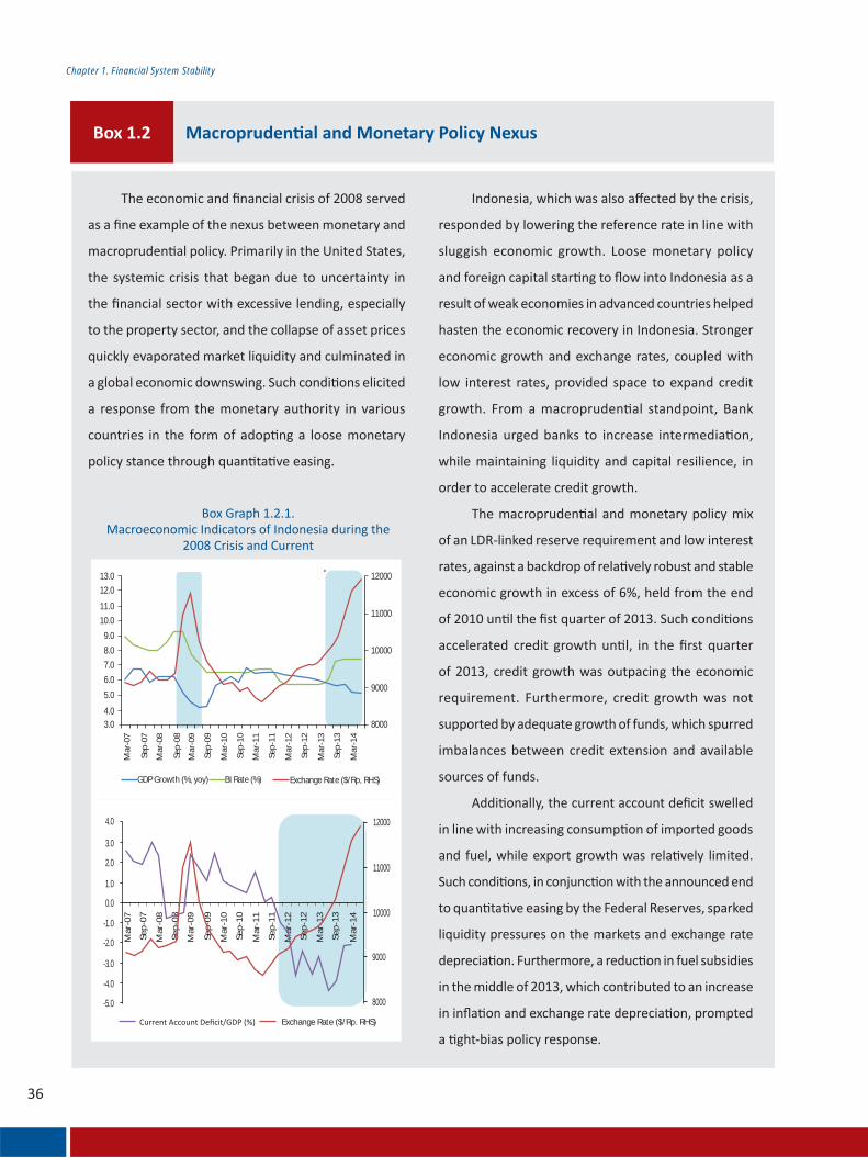
Box 1.2 Macropruden al and Monetary Policy Nexus
13.0 12000
11000
10000
9000
8000
12.0
11.0
10.0
9.0
8.0
7.0
6.0
5.0
4.03.0
GDP Growth (%, yoy) Exchange Rate ($/Rp, RHS)BI Rate (%)
Mar
-07
Sep-
07
Mar
-08
Sep-
08
Mar
-09
Sep-
09
Mar
-10
Sep-
10
Mar
-11
Sep-
11
Mar
-12
Mar
-13
Sep-
13
Mar
-14
Sep-
12
3.0
4.0
Exchange Rate ($/Rp. RHS)
Mar
-07
Sep
-07
Mar
-08
Sep
-08
Mar
-09
Sep
-09
Mar
-10
Sep
-10
Mar
-11
Sep
-11
Mar
-12
Mar
-13
Sep
-13
Mar
-14
Sep
-12
2.0
1.0
0.0
-1.0
-2.0
-3.0
-4.0
-5.0
12000
11000
10000
9000
8000

Chapter 1. Financial System Stability
40.0 3.0
2.5
1.5
1.0
0.5
0.0
-0.5
-1.0
-1.5
-2.0
2.035.0
30.0
25.0
20.0
15.0
10.0
Sep-
01M
ar-0
2Se
p-02
Credit/GDP Gap (%, RHS) Credit/GDP (%) Trend
Mar
-03
Sep-
03M
ar-0
4Se
p-04
Mar
-05
Sep-
05M
ar-0
6Se
p-06
Mar
-07
Sep-
07M
ar-0
8Se
p-08
Mar
-09
Sep-
09M
ar-1
0Se
p-10
Mar
-11
Sep-
11M
ar-1
2Se
p-12
Mar
-13
Sep-
13M
ar-1
4Se
p-14
218
6
4
2
0
-2
-4
-6
-8
16
11
6
Deposit Growth Gap (%, RHS) Deposit Growth (%, yoy) Tren
1
2002
Q1
2002
Q4
2003
Q3
2004
Q2
2005
Q1
2005
Q4
2006
Q3
2007
Q2
2008
Q1
2008
Q4
2009
Q3
2010
Q2
2011
Q1
2011
Q4
2012
Q3
2013
Q2
2014
Q1
2014
Q4

Chapter 1. Financial System Stability
Box 1.3 The Importance of Macropruden al Regula on and Supervision
Chapter 1. Financial System Stability

Chapter 1. Financial System Stability
st

41
Chapter 2. Financial Markets
Financial Markets
Chapter 2

42
Chapter 2. Financial Markets
This page is intentionally left blank
43
Chapter 2. Financial Markets
2.1 FINANCIAL MARKET RISKS
Domestic economic growth, which outpaced the
global economy, garnered investor confidence and
catalysed domestic financial market activity, coupled with
less intense financial market risks during the first semester
of 2014. Nonetheless, several potential risks continued to
demand vigilance in light of macroeconomic fundamentals
vulnerable to external imbalances. Furthermore,
uncertainty surrounding the global economy and domestic
political conditions affected near-term financial market
performance. Potential financial market risks emerged in
the guise of foreign capital flows as well as risks on the
money market, foreign exchange market, bond market,
stock market and mutual fund market.
National economic growth, which outperformed the global economy, helped stimulate domestic
financial market activity throughout the first semester of 2014. Such conditions were mirrored by a
maintained influx of foreign capital, greater transaction volume on the interbank money market (PUAB),
escalating interbank repurchase agreements (repo) and foreign exchange transactions, an increase in
outstanding tradeable government securities (SBN) and corporate bonds, gains on the IDX Composite
index as well as growth in managed investment funds. Furthermore, surging financial market activity
was accompanied by relatively well-mitigated risk, evidenced by declines in the interbank rate and its
volatility, a narrower spread between non-deliverable forwards and one-month onshore forwards,
lower SBN yields and volatility, less volatility on the stock market, an increase in net asset value
(NAV) as well as less volatility (beta coefficient) of mutual funds. Nevertheless, financial markets in
Indonesia remained vulnerable to potential risk stemming from external imbalances, primarily linked
to a possible sudden capital reversal.
2.1.1 Foreign Capital Flows
Growing investor confidence in the domestic
economy and financial markets was indicated by an
inflow of foreign purchases of domestic financial market
instruments, including Bank Indonesia Certificates (SBI),
tradable government securities (SBN), corporate bonds
and shares. On the SBI market, foreign holdings increased
from the beginning of the reporting semester to reach
Rp8.57 trillion in May 2014 before subsequently returning
to record an outflow of Rp3.87 trillion in June. In general,
however, foreign SBI holdings registered a net inflow
of Rp10.96 trillion. On the SBN market, foreign inflows
peaked at Rp20.15 trillion in May 2014, with a total value
for the reporting semester of Rp79.95 trillion. Concerning
the stock market, foreign inflows peaked in April 2014 at
Rp11.48 trillion, with a total inflow value of Rp48.07 trillion
Chapter2
Financial Markets
44
Chapter 2. Financial Markets
Source: Bloomberg, Bank Indonesia
Graph 2.1Non-Resident Flows: Shares, SBN & SBI
Source: Bank Indonesia
Graph 2.2Rupiah Interbank Money Market Performance
Source: Bank Indonesia
Graph 2.3Overnight Rupiah Interbank Rate
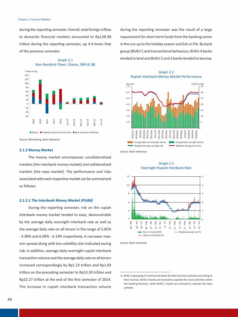
during the reporting semester. Overall, total foreign inflow
to domestic financial markets amounted to Rp138.98
trillion during the reporting semester, up 4.4 times that
of the previous semester.
during the reporting semester was the result of a large
requirement for short-term funds from the banking sector
in the run up to the holiday season and Eid-ul-Fitr. By bank
group (BUKU1) and transactional behaviour, BUKU 4 banks
tended to lend and BUKU 2 and 3 banks tended to borrow.
2.1.2 Money Market
The money market encompasses uncollateralised
markets (the interbank money market) and collateralised
markets (the repo market). The performance and risks
associated with each respective market can be summarised
as follows:
2.1.2.1 The Interbank Money Market (PUAB)
During the reporting semester, risk on the rupiah
interbank money market tended to ease, demonstrable
by the average daily overnight interbank rate as well as
the average daily rate on all tenors in the range of 5.85%
- 5.90% and 6.09% - 6.19% respectively. A narrower max-
min spread along with less volatility also indicated easing
risk. In addition, average daily overnight rupiah interbank
transaction volume and the average daily rate on all tenors
increased correspondingly by Rp1.23 trillion and Rp1.69
trillion on the preceding semester to Rp13.30 trillion and
Rp22.27 trillion at the end of the first semester of 2014.
The increase in rupiah interbank transaction volume
-60
-40
-20
0
20
40
60
80
100
120
140
2009
2010
2011
2012
2013
Jan-
14
Feb-
14
Mar
-14
Apr-
14
Mei
-14
Jun-
14
Trillion of Rp
Shares Tradeable Government Securities Bank Indonesia Certificates
7.0 35
30
25
20
15
10
5
--
6.0
5.0
4.0
3.0
2.0
1.0
2010
/Jan
2010
/Apr
2010
/Jul
2010
/Okt
2011
/Jan
2011
/Apr
2011
/Jul
2011
/Okt
2012
/Jan
2012
/Apr
2012
/Jul
2012
/Okt
2010
/Jan
2010
/Apr
2010
/Jul
2010
/Okt
2010
/Jan
2010
/Apr
Percent Trillion of Rp
Average Daily non-overnight volumeWeighted average overnight rate
Average Daily overnight volumeWeighted average of all rates
Ags - 08
Jan - 09
Jun - 09
Nov - 09
Apr - 10
Sep - 10
Feb - 11
Jul - 11
Dec - 11
Mar - 12
Oct - 12
Mar - 13
Ags - 13
Jan - 14
Jun - 14
512
10
8
6
4
2
4
3
2
1
0
Max-min Spread (RHS) Weighted average rate (%)Highest Lending Rate (%)
1) BUKU is grouping of commercial banks by their business activities according to their licenses. BUKU 4 banks are licensed to operate the most activities within the banking business, while BUKU 1 banks are licensed to operate the least activites.

45
Chapter 2. Financial Markets
foreign exchange interbank money market volume
increased moderately by US$3.3 million to US$492.22
million. The large decline in average daily transaction
volume on the foreign exchange interbank money market,
accompanied by an increase on the rupiah interbank
money market, demonstrated that the banking sector
favoured the rupiah interbank money market to manage
its short-term funds. By bank group and transactional
behaviour, BUKU 3 and 4 banks were lenders, while BUKU
2 banks were borrowers.
Source: Bank Indonesia
Graph 2.4Rupiah Interbank Rate Volatility
Source: Bank Indonesia
Graph 2.5Rupiah Interbank Transactional Behaviour
Source: Bank Indonesia
Graph 2.6Foreign Exchange Interbank Money Market
Source: Bank Indonesia
Graph 2.7Overnight Foreign Exchange Interbank Rate
Congruent with less risk on the rupiah interbank
money market, risk on the foreign exchange interbank
money market also eased, reflected by the average daily
overnight foreign exchange interbank rate and the average
daily rate on all tenors in the range of 0.12% - 0.15% and
0.14% - 0.18% respectively. Narrower spread between
the max-min overnight interbank rate, coupled with less
volatility, was also evidence of less risk. Average daily
foreign exchange interbank money market transaction
volume of all tenors dropped US$77.40 million on the
preceding semester to US$667.43 million at the end of the
first semester of 2014. Meanwhile, average daily overnight
Jan-
13Fe
b-13
Mar
-13
Apr-1
3
May
-13
Jun-
13Ju
l-13
Aug-
13
Sep-
13
Oct
-13
Nov
-13
Dec-
13
Jan-
14Fe
b-14
Mar
-14
Apr-1
4
May
-14
Jun-
14
90% 8.0
7.5
7.0
6.5
6.0
5.5
5.0
4.5
4.0
80%
70%
60%
50%
40%
30%
20%
10%
0%
BI Rate (RHS)
Lending Facility (RHS)
O/N Interbank Rate (RHS)O/N Rp Interbank VolatilityDeposit Facility (RHS)
2012/Jan
2012/Mar
2012/May
2012/Jul
2012/Sep
2012/Nov
2013/Jan
2013/Mar
2013/May
2013/Jul
2013/Sep
2013/Nov
2014/Jan
2014/Mar
2014/May
150
100
50
0
-50
-100
-150
Buku 4
Trillions of Rp
Buku 3 Buku 2 Buku 1
1,6000.35
Average Daily Non-O/N Volume
0.30
0.25
0.20
0.15
0.10
0.05
-
1,400
1,200
1,000
800
600
400
200
-
Millions of USDPercent
naJ/0102
rpA/0102
l uJ/0102
tgA/0102naJ/1102
r pA/1102
l uJ/1102
tgA/1102naJ/2102
r pA/2102
l uJ/2102
tgA/2102naJ/3102
r pA/3102
l uJ/3102
tgA/3102naJ/4102
r pA/4102
Weighted Average O/N RateAverage Daily O/N VolumeWeighted Average of All Rates
Max-min Spread (RHS) Weighted average rate (%)
0.50 1.8
1.6
1.4
1.2
1
0.8
0.6
0.4
0.2
0
0.45
0.40
0.35
0.30
0.25
0.20
0.15
0.10
0.05
0.00Nov - 08Feb - 09M
ay - 09Ags- 09Nov - 09Feb - 10M
ay - 10Ags- 10Nov - 10Feb - 11M
ay - 11Ags- 11Nov - 11Feb - 12M
ay - 12Ags- 12Nov - 12Feb - 13M
ay - 13
Feb - 14M
ay - 14
Ags- 13Nov - 13
Highest Lending Rate (%)
46
Chapter 2. Financial Markets
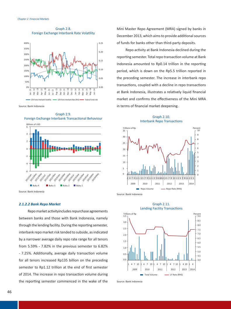
2.1.2.2 Bank Repo Market
Repo market activityincludes repurchase agreements
between banks and those with Bank Indonesia, namely
through the lending facility. During the reporting semester,
interbank repo market risk tended to subside, as indicated
by a narrower average daily repo rate range for all tenors
from 5.59% - 7.82% in the previous semester to 6.82%
- 7.25%. Additionally, average daily transaction volume
for all tenors increased Rp135 billion on the preceding
semester to Rp1.12 trillion at the end of first semester
of 2014. The increase in repo transaction volume during
the reporting semester commenced in the wake of the
Source: Bank Indonesia
Graph 2.8.Foreign Exchange Interbank Rate Volatility
Source: Bank Indonesia
Graph 2.9.Foreign Exchange Interbank Transactional Behaviour
Source: Bank Indonesia
Graph 2.10.Interbank Repo Transactions
Source: Bank Indonesia
Graph 2.11.Lending Facility Transactions
Mini Master Repo Agreement (MRA) signed by banks in
December 2013, which aims to provide additional sources
of funds for banks other than third-party deposits.
Repo activity at Bank Indonesia declined during the
reporting semester. Total repo transaction volume at Bank
Indonesia amounted to Rp0.14 trillion in the reporting
period, which is down on the Rp5.5 trillion reported in
the preceding semester. The increase in interbank repo
transactions, coupled with a decline in repo transactions
at Bank Indonesia, illustrates a relatively liquid financial
market and confirms the effectiveness of the Mini MRA
in terms of financial market deepening.
O/N Forex Interbank Rate (RHS) Federal Funds rateO/N Forex Interbank Volatility
Jan -
13
Feb -
13M
ar - 1
3
Apr -
13M
ay - 1
3
Jun -
13
Jan -
14
Feb -
14M
ar - 1
4
Apr -
14M
ay - 1
4
Jun -
14
Jul -
13
Aug -
13
Sep -
13Oc
t - 13
Nov -
13
Dec -
13
400% 0.25
0.20
0.15
0.10
0.05
0.00
350%
300%
250%
200%
150%
100%
50%
0%
6Billions of USD
4
2
0
-2
-4
-6
2012
/Jan
2012
/Mar
2012
/May
2012
/Jul
2012
/Sep
2012
/Nov
2013
/Jan
2013
/Mar
2013
/May
2014
/Jan
2014
/Mar
2014
/May
2013
/Jul
2013
/Sep
2013
/Nov
Buku 4 Buku 3 Buku 2 Buku 1
35Trillions of Rp Percent
9
10
8
7
6
5
4
3
2
1
0
30
25
20
15
10
5
0
2 4 7 9 11 1 3 5 7 9 11 1 3 5 8 1012 3 5 7 9 11 1 3 5 7 9 11 1 3 5
2009 2010 2011 2012 2013 2014
Repo Volume Repo Rate (RHS)
3.5Trillions of Rp Percent
9.0
8.5
8.0
7.5
7.0
6.5
6.0
5.5
5.0
4.5
4.0
3.0
2.5
2.0
1.5
1.0
0.5
0.0
1 4 7 10 1 4 7 10 1 4 7 10 1 4 7 10 1 4 10 1 4
2009 2010 2011 2012 2013 2014
Total Volume LF Rate (RHS)

47
Chapter 2. Financial Markets
3.1.3 Foreign Exchange Market
Risk also eased on the foreign exchange market,
amongst others reflected by a narrower spread between
non-deliverable forwards and one-month onshore
forwards. Furthermore, adequate liquidity on the foreign
exchange market also signalled less risk. Total foreign
exchange transaction volume increased from US$262.03
billion in the second semester of 2013 to USD322.17 in
the reporting period.
In terms of composition, spot transactions
dominated the domestic foreign exchange market with a
volume accounting for 67.31% of total foreign exchange
transactions. Meanwhile, the portion of forward and swap
transactions amounted to 5.45% and 27.24% respectively.
The relatively small share of forward and swap transactions
in comparison to spot transactions is an indicator of a
shallow domestic foreign exchange market that requires
further financial deepening efforts.
Source: Bank Indonesia, Bloomberg, processed
Graph 2.12.Foreign Exchange Market Risk Premium
Source: Bank Indonesia, Bloomberg, processed
Graph 2.13.Swap Transaction Volume
Source: Bank Indonesia
Graph 2.14.Domestic Foreign Exchange Market Volume
Source: Bank Indonesia
Graph 2.15.Foreign Exchange Transaction Volume Trend
800Point Rp
13,000
12,500
12,000
11,500
11,000
10,500
10,000
9,500
9,000
8,500
8,000
600
400
200
-200
-400
-600
-800
Jan-
12
Mar
-12
May
-12
Jul-1
2
Sep-
12
Nov
-12
Jan-
13
Mar
-13
May
-13
Jan-
14
Mar
-14
May
-14
Jul-1
3
Sep-
13
Nop
-13
0
Spread NDF-FWD 1B RRH 10D Spread NDF 1B (RHS)
8.0%
7.0%120
100
80
60
40
20
Jun-12 Dec-12 Dec-13Jun-13 Jun-14
6.0%
5.0%
4.0%
3.0%
2.0%
1.0%
0.0%
Total Vol. Semesteran (RHS) Premi Swap Broker O/N
Billions of USD
Premi Swap Broker 1B Premi Swap Broker 3BPremi Swap Broker 6B
70
60
50
40
30
20
10
OPTION
0
2010
/Jan
2010
/Mar
2010
/May
2010
/Jul
2010
/Sep
2010
/Nov
2011
/Jan
2011
/Mar
2011
/May
2011
/Jul
2011
/Sep
2011
/Nov
2012
/Jan
2012
/Mar
2012
/May
2012
/Jul
2012
/Sep
2012
/Nov
2013
/Jan
2013
/Mar
2013
/May
2013
/Jul
2013
/Sep
2013
/Nov
2014
/Jan
2014
/Mar
2014
/May
Billions of USD
FORWARD SWAP SPOT
65
60
55
50
45
40
35
301 2 3 4 5 6 7 8 9 10 11 12
Billions of USD
2011 2012 2013 2014

48
Chapter 2. Financial Markets
2.1.4 Bond Market
On the bond market, economic stimulus packages
and low interest rates in a number of advanced countries
were important factors leading to an influx of foreign
capital into government securities (SBN), increasing from
Rp44.46 trillion in the second semester of 2013 to Rp79.95
trillion in the reporting semester. Foreign purchases of SBN
occurred on the secondary market as well as issuances on
the primary market by the government. Accordingly, the
portion of foreign SBN holdings increased from 32.54% on
the preceding semester to 35.66%.
Source: Bank Indonesia
Graph 2.16.Foreign Net Flow to SBN and IDMA Index
Source: CEIC
Graph 2.17.SBN Holdings
The surge in foreign inflow to SBN prompted higher
SBN prices, with the IDMA index rallying to 96.65 points
from 95.46 points in the previous semester. Meanwhile,
SBN market risk eased as yield and volatility decreased.
SBN yield for tenors of 10 years dropped 28 bps to 8.09%,
accompanied by a 46 bps decline in volatility to 2.18%,
one of the lowest in Asia.
Source: Bloomberg, processed
Source: Bloomberg, processed
Table 2.1.10-Year SBN Yield and Regional Yields
Table 2.2.10-Year SBN Volatility and Regional Volatility (%)
INDO INDI THAI MAL PHILJun-13 7.06 7.69 3.63 3.72 4.07Jul-13 8.52 8.86 4.13 4.04 3.18
Aug-13 8.32 8.97 3.87 3.76 3.61Sep-13 5.93 8.31 3.50 3.55 4.65Oct-13 5.65 8.33 3.30 3.43 4.67
Nov-13 8.59 9.09 3.91 4.30 3.35Dec-13 8.37 9.17 3.80 4.20 3.42Jan-14 8.81 8.86 3.78 4.22 4.24Feb-14 8.34 9.06 3.54 4.10 4.38Mar-14 7.99 9.11 3.51 4.01 3.85Apr-14 7.86 9.02 3.42 3.95 3.98
May-14 7.95 8.77 3.57 3.96 3.61Jun-14 8.09 8.58 3.57 3.93 3.78
INDO IND THAI MAL PHIJun-13 8.69 5.36 9.56 8.19 16.13 Jul-13 17.47 26.20 3.16 7.53 8.99
Aug-13 11.78 10.63 7.24 2.78 1.77 Sep-13 12.97 5.38 8.23 6.41 6.51 Oct-13 17.04 2.81 3.02 4.22 6.46 Nov-13 4.22 8.23 5.78 6.88 2.74 Dec-13 2.64 7.95 2.62 3.03 14.06 Jan-14 9.93 8.78 1.77 4.91 12.75 Feb-14 5.23 5.66 3.22 2.41 3.70 Mar-14 4.03 3.11 3.37 2.65 5.74 Apr-14 1.64 5.19 3.35 1.39 2.09
May-14 2.17 6.12 3.20 3.31 2.82 Jun-14 2.18 5.32 1.50 0.98 3.23
90Trillions of Rp Point
115
80
70
60
50
40
30
20
10
2009
2010
2011
2012
2013
Jan-
14
Feb-
14
Mar
-14
Apr-1
4
May
-14
Jun-
14
0
110
105
100
95
90
85
80
SBN IDMA (RHS)
1200Trillions of Rp
1000
800
600
400
200
0Jun-11 Dec-11 Jun-12 Dec-12 Jun-13 Jun-14Dec-13
Others Securities Pension Funds Foreign
Insurers Mutual Funds Central Bank Banks
49
Chapter 2. Financial Markets
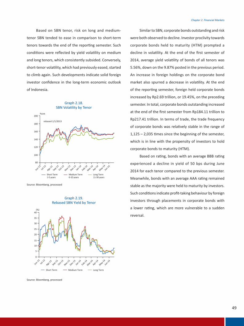
Based on SBN tenor, risk on long and medium-
tenor SBN tended to ease in comparison to short-term
tenors towards the end of the reporting semester. Such
conditions were reflected by yield volatility on medium
and long tenors, which consistently subsided. Conversely,
short-tenor volatility, which had previously eased, started
to climb again. Such developments indicate solid foreign
investor confidence in the long-term economic outlook
of Indonesia.
Source: Bloomberg, processed
Graph 2.18.SBN Volatility by Tenor
Source: Bloomberg, processed
Graph 2.19.Rebased SBN Yield by Tenor
Similar to SBN, corporate bonds outstanding and risk
were both observed to decline. Investor proclivity towards
corporate bonds held to maturity (HTM) prompted a
decline in volatility. At the end of the first semester of
2014, average yield volatility of bonds of all tenors was
5.56%, down on the 9.87% posted in the previous period.
An increase in foreign holdings on the corporate bond
market also spurred a decrease in volatility. At the end
of the reporting semester, foreign held corporate bonds
increased by Rp2.69 trillion, or 19.45%, on the preceding
semester. In total, corporate bonds outstanding increased
at the end of the first semester from Rp184.11 trillion to
Rp217.41 trillion. In terms of trade, the trade frequency
of corporate bonds was relatively stable in the range of
1,125 – 2,035 times since the beginning of the semester,
which is in line with the propensity of investors to hold
corporate bonds to maturity (HTM).
Based on rating, bonds with an average BBB rating
experienced a decline in yield of 50 bps during June
2014 for each tenor compared to the previous semester.
Meanwhile, bonds with an average AAA rating remained
stable as the majority were held to maturity by investors.
Such conditions indicate profit-taking behaviour by foreign
investors through placements in corporate bonds with
a lower rating, which are more vulnerable to a sudden
reversal.
200Point
rebased 1/1/2013
1-5 years 6-10 years 11-30 years
180
160
140
120
100
80
Jun-13Jul-1
3
Ags-13
Sep-13
Oct-13
Nov-13
Dec-13
Jan-14
Feb-14
Mar-14
Apr-14
May-14
Jun-14
Short Term Medium Term Long Term
40(%)
35
30
25
20
15
10
5
0
Ags-13
Sep-13
Oct-13
Nov-13
Dec-13
Jan-14
Feb-14
Mar-14
Apr-14
May-14
Jun-14Jun-13
Jul-13
Short Term Medium Term Long Term

50
Chapter 2. Financial Markets
2.1.5 Stock Market
On the stock market during the reporting period,
the JCI (Indonesian Stock Market composite index) rallied
while risk eased as volatility declined both as an aggregate
and by sector. Optimism surrounding a surge in economic
activity linked to the presidential election as well as sound
financial statements of domestic issuers helped stabilise
foreign capital inflows throughout the first semester.
Stock indices in Indonesia and the Philippines, which
share similar economic structures and issues in the eyes
of foreign investors, led gains on regional stock exchanges.
Source: Bloomberg, processed
Graph 2.20.Corporate Bond Volatility by Tenor
Source: Financial Services Authority (OJK)
Graph 2.23.Corporate Bond Trade Frequency
Source: Bloomberg, processed
Graph 2.21.Rebased Corporate Bond Yield by Tenor
Source: CEIC, processed
Graph 2.24.Foreign Net Flow and Holdings of Corporate Bonds
Source: Indonesia Bond Pricing Agency (IBPA)
Graph 2.22.Corporate Bond Yield Curve
40(%)
35
30
25
20
15
10
5
0
Ags-13
Sep-13
Oct-13
Nov-13
Dec-13
Jan-14
Feb-14
Mar-14
Apr-14
May-14
Jun-14Jun-13
Jul-13
Short Term Medium Term Long Term
Short Term: 1-5 yearsMedium Term: 6-10 yearsLong Term: 11-30 years
145Point
135
140
130
125
120
115
105
100
Jun-13Jul-1
3
Ags-13
Sep-13
Oct-13
Nov-13
Dec-13
Jan-14
Feb-14
Mar-14
Apr-14
May-14
Jun-14
110
Short Term Medium Term Long Term
16(%)
15
14
13
12
11
10
9
8
7
61
SBN Jun14
AAA Dec13
2 3 4 5 6 7 8 9 10
SBN Dec13
BBB Jun14
AAA Jun14
BBB Dec13
180 230Trillions of Rp
2007 2008 2009 2010 2011 2012 2013 2014
1 2 3 4 5 6
thousand times
Corporate Bond Frequency
210
190
170
150
130
110
90
70
50
30
160
140
120
100
80
60
40
20
0
SUN Frequency Outstanding Corporate Bonds (RHS)
7
2010 2011 2012 2013 2014
1 2 3 4 5 6
18
16
14
12
10
8
6
4
2
0
Trillions of Rp Trillions of Rp
6
5
4
3
2
1
0
(1)
Outstanding Foreign Holdings (RHS)Net Flow

51
Chapter 2. Financial Markets
Less risk on the domestic stock market was also
inextricably tied to less risk on regional and global stock
markets. As presented in subsection 1.1 concerning
Regional and Global Market Performance, the volatility of
several global stock market indices was observed to decline
at the end of the first semester compared to yearend 2013
despite escalating due to heightened political tensions
along the Russia-Ukraine border. A decrease in global
volatility primarily stemmed from improved investor
sentiment regarding the crisis in Europe after sources of
the crisis, such as Greece, Ireland, Spain, Portugal and Italy
enjoyed a bump in their respective credit rating. In the case
of Greece, government securities were reissuedfor the
first time since 2010. Meanwhile, stock market volatility
in Indonesia also eased in line with a number of other
markets in the region.
Source: Bloomberg, processed
Graph 2.25.Regional Stock Market Performance
Source: Bloomberg, processed
Graph 2.27.Flow to Shares and JCI
Source: Bloomberg, processed
Graph 2.26.Regional Stock Market Volatility
Source: Bloomberg, processed
Table 2.3.Heat Map of Index Volatility by Sector
2012TW 4 TW 1 TW 2 TW 3 TW 4 TW 1 TW 2
IDX Composite 9.39 12.78 22.75 31.04 17.63 18.13 14.30Financial 15.76 17.28 25.58 37.01 23.24 24.66 18.60Agriculture 16.65 14.65 22.79 32.19 19.01 24.91 17.13Basic Industry 14.06 17.20 28.94 43.96 25.15 25.30 22.35Consumption 19.56 16.57 30.87 40.22 21.32 18.81 15.28Property 12.90 22.29 31.57 43.93 23.11 28.19 20.16Mining 14.64 22.75 22.22 31.85 19.48 18.58 17.10Infrastructure 14.13 15.97 28.22 31.29 20.63 20.98 17.29Trade 11.15 14.61 23.40 27.69 13.76 12.99 14.18Miscellaneous Industries 28.06 23.78 37.45 45.79 31.39 31.02 22.14
2013 2014
Indonesia Thailand Malaysia the Philippines
Jan-
13
Feb-
13
Mar
-13
Apr
-13
May
-13
Jun-
13
Jul-1
3
Ags
-13
Sept
-13
Jan-
14
Feb-
14
Mar
-14
Apr
-14
May
-14
Jun-
14
Oct
-13
Nov
-13
Dec
-13
130Point
125
120
115
110
105
100
95
9085
80
Indonesia Thailand the PhilippinesMalaysia Singapore
Jun-
13
Jul-1
3
Aug-
13
Sep-
13
Jan-
14
Feb-
14
Mar
-14
Apr-
14
May
-14
Jun-
14
Oct
-13
Nov
-13
Dec
-13
90Trillions
80
70
60
50
40
30
20
10
0
5000PoinRp (T)
4500
4000
3500
3000
2500
2000
30
25
10
0
-10
-20
-30
Saham JCI (skala kanan)
2009
2010
2011
2012
2013
Jan-
14
Feb-
14
Mar
-14
Apr-
14
Mei
-14
Jun-
14

52
Chapter 2. Financial Markets
Based on share type, the role of non-LQ45 shares
expanded in comparison to the shares of LQ45 companies,
as demonstrated by the portion of LQ45 that shrank to 65%
in June 2014 from 80% at the end of 2009. Nevertheless,
compared to the portion at yearend 2013, little change
has occurred. As derivatives increasingly crowd the stock
market, for instance mutual funds, their contribution helps
extend the market share of non-LQ45 shares. Furthermore,
the expanding role of non-LQ45 shares is also attributable
to the market’s view that such shares are under-priced and
therefore attractive to foreign investors. Such conditions
demand vigilance in order to prevent a sudden reversal.
2.1.6 Mutual Funds
During the reporting period, risk on the three main
investment fund markets (money market, stock market and
SBN market) was observed to decline as the risk associated
with each respective underlying asset also eased, as
reflected by less volatility. Less risk was accompanied by
stronger growth of managed funds. On the other hand,
Net Asset Value (NAV) increased in the first semester by
9.06% to Rp209.98 trillion compared to Rp192.54 trillion in
the preceding period. Year on year, NAV growth remained
positive during the first semester of 2014.Source: Bloomberg, processed
Graph 2.28.JCI Share Trade Frequency
Source: Bloomberg, processed
Graph 2.29.JCI and LQ45 Capitalisation
Source: Financial Services Authority (OJK) report
Graph 2.31.Mutual Fund NAV Volatility by Type
Source: Bloomberg, processed
Graph 2.30.JCI and LQ45 Price Performance
100%
90%
80%
70%
60%
50%
40%
30%
20%
10%
0%
Feb-
08
Jun-
08O
ct-0
8Fe
b-09
Jun-
09O
ct-0
9Fe
b-10
Jun-
10O
ct-1
0Fe
b-11
Jun-
11O
ct-1
1Fe
b-12
Jun-
12O
ct-1
2Fe
b-13
Jun-
13O
ct-1
3Fe
b-14
Jun-
14
Non LQ45 LQ45
6.000Trillions of Rp
80%
75%
70%
65%
60%
55%
50%
45%
40%
5.000
4.000
3.000
2.000
1.000
IDX Composite Capitalisation
2004
2005
2006
2007
2008
2009
2010
2011
2012
2013
2014
LQ45 Capitalisation LQ45 Share (RHS)
1400
1200
1000
800
600
400
200
Spread (RHS) JCI
2004 2005 2006 2007 2008 2009 2010 2011 2012 2013 2014
0
rebased 1/1/2000 500bps
400
300
200
100
0
-100
-200
LQ45
60(%)
50
40
30
20
10
Fixed-income funds
0
Jan-13
Feb-13
Mar-13
Apr-13
May-13
Jun-13
Jan-14
Feb-14
Mar-14
Apr-14
May-14
Jun-14
Jul-1
3
Aug-13
Sep-13
Oct-13
Nov
-13
Dec-13
Discretionary funds Equity funds

53
Chapter 2. Financial Markets
50
48
46
44
42
40
38
36
34
32
30
1 2 3 4 5 6 7 8 9 10 11 12
2011 2012 2013 2014
Trillions of Rp45
40
35
30
25
20
1 2 3 4 5 6 7 8 9 10 11 12
2011 2012 2013 2014
Trillions of Rp
Total Mutual Funds (RHS) NAV (trillions of Rp) Units in Circulation (millions)
1 4 7 10
2008
250 900
800
700
600
500
400
300
200
100
0
200
150
100
50
01 4 7 10
2009
1 4 7 10
2010
1 4 7 10
2011
1 4 7 10
2012
1 4 7 10
2013
1 4
2014
A favourable mutual fund market was also evidenced
in the first semester by a tendency that followed seasonal
trends over the past three years. By type, equity funds
continued to dominate the NAV of mutual funds with a
43.39% share, followed by protected funds with 20.38%.
Source: Financial Services Authority (OJK) report
Graph 2.32.Growth of Mutual Funds (yoy)
Graph 2.34.NAV trend ofMutual Funds by Type
Source: Financial Services Authority (OJK) report
Graph 2.33.Position of Mutual Funds
40%
35%
30%
25%
20%
15%
10%
5%
0%
-5%
-10%
NAV Units in Circulation Total Mutual Funds
1 2 3 4 5 6 7 8 9 10 1112
2012
1 2 3 4 5 6 7 8 9 10 1112
2013
1 2 3 4 5 6
2014
Trillions of Rp100
90
80
70
60
50
40
1 2 3 4 5 6 7 8 9 10 11 12
2011 2012 2013 2014
16
15
14
13
12
11
10
9
8
7
6
1 2 3 4 5 6 7 8 9 10 11 12
2011 2012 2013 2014
Trillions of RpEquity funds Money market funds
Protected funds Fixed-income funds
The market share of equity funds increased compared to
the previous semester, indicating growing investor interest
in equity funds as share performance increased. Nominally,
the net asset value of nearly all types of investment funds
increased.
Source: Financial Services Authority (OJK) report, processed

54
Chapter 2. Financial Markets
pushing up returns on equity funds and balanced funds.
Such conditions were reflected in the majority of equity
funds with positive excess returns at the end of the first
semester. Maintained SBN prices offset further gains in
discretionary funds and ensured relatively stable returns
on fixed-income funds.
Concerning individual investment fund products, a
significant decline in risk was experienced by equity funds
as the beta coefficient for the majority of equity funds
dropped, which precipitated JCI gains along with less NAV
volatility. Concerning balanced funds, fixed-income funds
and money market funds, the majority of beta coefficients
remained below 1 in line with the natural characteristics of
short-term bonds and securities as underlying assets with
low price volatility compared to equity funds.
Sumber : Bloomberg, diolah
In general, mutual funds experienced higher
returns and less risk during the reporting semester. The
JCI rallied 12.7% during the first semester of 2014, hence
Graph 2.36.Risk Profile of Mutual Fund Products
Source: Financial Services Authority (OJK) report
Graph 2.35.NAV of Mutual Funds by Type
Trillions of Rp
220200
180160140120100
80
604020
0
Jan
Apr
Jul
Oct
2009
Jan
Apr
Jul
Oct
2010
Jan
Apr
Jul
Oct
2011
Jan
Apr
Jul
Oct
2012
Jan
Apr
Jul
Oct
2013
Jan
Apr
2014
Equity funds Money market funds Discretionary FundsFixed-income funds Protected funds Others
Money Market Funds Fixed-income Funds
Discretionary Funds Equity Funds

55
Chapter 2. Financial Markets
2.2 THE FINANCIAL MARKET AS A SOURCE OF NON-BANK FINANCING
Financing activity through non-bank financial
institutions, in general, increased from Rp65.77 trillion at
the end of the second semester of 2013 to Rp71.51 trillion
in the reporting period. The increase primarily affected the
capital market, which is observable from the number of
issuers instituting initial public offerings (IPO) and rights
issues in the first semester of 2014 with a nominal value of
Rp30.43 trillion. Correspondingly, issuances of corporate
bonds also increased during the first semester, totalling
Rp28.18 trillion compared to just Rp13.37 trillion in the
previous period.
Tenacious investor interest in domestic financial
market assets along with sustained economic growth
provided momentum for the corporate sector to seek
alternative sources of financing outside of the banking
sector. Furthermore, a wide spread between bank lending
rates and the reference rate also boosted corporate
interest in terms of issuing bonds. The government also
responded by implementing continuous bond policy in
2010, which simplified the issuance of bonds and reduced
dependence on bank financing.
Source: Financial Services Authority (OJK) report
Source: Financial Services Authority (OJK), Bank Indonesia, Bloomberg, processed
Graph 2.37.Nominal Value of Bonds
Trillions of RP2014
sem I sem II sem I
A. Bank Credit 327.92 434.25 507.77 251.26 333.75 175.29B. Non-Bank Financing 156.76 158.96 154.32 95.25 65.77 71.51 B1. Capital Market 112.95 100.01 97.57 76.48 38.56 58.61
- IPO and Rights Issues 76.35 54.28 30.10 32.35 25.19 30.43 - Corporate Bonds 36.60 45.74 67.46 44.13 13.37 28.18
B2. Finance Companies 43.81 58.95 56.75 18.77 27.21 12.90Total 484.68 593.21 662.09 346.51 399.52 246.79
2010 2011 20122013
Description
Table 2.4.Bank and Non-Bank Financing
Concerning initial public offerings (IPO), there are
typically between 12 and 30 new issuers each year. During
the first semester of 2014, however, share issuances only
totalled Rp16.75 trillion, less than half the total issued in
2013 (Rp57.54 trillion). On the other hand, slower bank
credit growth did not seem to trigger a substitution of bank
credit for shares, reflecting increasingly limited domestic
sources of funds.
14 30
25
20
15
10
5
0
(%)Trillions of Rp
12
10
8
6
4
2
0
-2
Corporate bonds (trillions of Rp)
BI Rate (%)
Working Capital Credit (%)
YOY Exchange Rate (RHS)
-4
Jan-13
Feb-13
Mar-13
Apr-13
May-13
Jun-13
Jan-14
Feb-14
Mar-14
Apr-14
May-14
Jun-14
Jul-1
3
Ags-13
Sep-13
Oct-13
Nov
-13
Dec-13
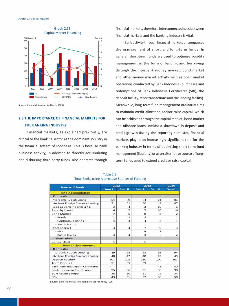
56
Chapter 2. Financial Markets
2.3 THE IMPORTANCE OF FINANCIAL MARKETS FOR
THE BANKING INDUSTRY
Financial markets, as explained previously, are
critical to the banking sector as the dominant industry in
the financial system of Indonesia. This is because bank
business activity, in addition to directly accumulating
and disbursing third-party funds, also operates through
Source: Financial Services Authority (OJK)
Graph 2.38.Capital Market Financing
60 8
7
6
5
4
3
2
1
0
50
40
30
20
10
02007 2008 2009 2010 2011 2012 2013 2014
Trillions of Rp Percent
IPORights Issues GDP (RHS)
Working Capital Credit (yoy)New Issuers
financial markets, therefore interconnectedness between
financial markets and the banking industry is vital.
Bank activity through financial markets encompasses
the management of short and long-term funds. In
general, short-term funds are used to optimise liquidity
management in the form of lending and borrowing
through the interbank money market, bond market
and other money market activity such as open market
operations conducted by Bank Indonesia (purchases and
redemptions of Bank Indonesia Certificates (SBI), the
deposit facility, repo transactions and the lending facility).
Meanwhile, long-term fund management ordinarily aims
to maintain credit allocation and/or raise capital, which
can be achieved through the capital market, bond market
and offshore loans. Amidst a slowdown in deposit and
credit growth during the reporting semester, financial
markets played an increasingly significant role for the
banking industry in terms of optimising short-term fund
management (liquidity) or as an alternative source of long-
term funds used to extend credit or raise capital.
Table 2.5.Total Banks using Alternative Sources of Funding
2014Sem I Sem II Sem I Sem II Sem I
Fund AccumulationI. DomesticInterbank Rupiah Loans 54 79 74 81 81 Interbank Foreign Currency Lending 51 51 50 48 47 Repo at Bank Indonesia / LF 3 4 3 10 1 Repo by banks 6 7 7 10 16 Bond Market 7 6 8 3 2 - Bonds 2 2 3 1 - Continuous Bonds 4 4 4 3 1 - Sukuk Bonds 1 1 Stock Market 3 4 7 9 3 - IPO 4 2 1 - Rights Issues 3 4 3 7 2 II. InternationalBonds (USD) 1 1
Fund DisbursementsI. DomesticInterbank Rupiah Lending 89 95 93 95 94 Interbank Foreign Currency Lending 48 47 48 49 45 Deposit Facility 107 105 110 100 107 Term Deposit 51 65 39 - - Bank Indonesia Deposit Certificates - - - 43 50 Bank Indonesia Certificates 95 86 91 98 98 SUN Reverse Repo 38 30 31 25 36 SBN 43 51 52 58 50
Source of Funds 2012 2013
Source: Bank Indonesia, Financial Services Authority (OJK)
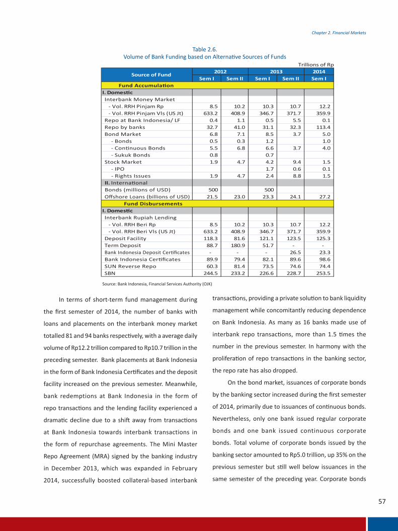
57
Chapter 2. Financial Markets
In terms of short-term fund management during
the first semester of 2014, the number of banks with
loans and placements on the interbank money market
totalled 81 and 94 banks respectively, with a average daily
volume of Rp12.2 trillion compared to Rp10.7 trillion in the
preceding semester. Bank placements at Bank Indonesia
in the form of Bank Indonesia Certificates and the deposit
facility increased on the previous semester. Meanwhile,
bank redemptions at Bank Indonesia in the form of
repo transactions and the lending facility experienced a
dramatic decline due to a shift away from transactions
at Bank Indonesia towards interbank transactions in
the form of repurchase agreements. The Mini Master
Repo Agreement (MRA) signed by the banking industry
in December 2013, which was expanded in February
2014, successfully boosted collateral-based interbank
transactions, providing a private solution to bank liquidity
management while concomitantly reducing dependence
on Bank Indonesia. As many as 16 banks made use of
interbank repo transactions, more than 1.5 times the
number in the previous semester. In harmony with the
proliferation of repo transactions in the banking sector,
the repo rate has also dropped.
On the bond market, issuances of corporate bonds
by the banking sector increased during the first semester
of 2014, primarily due to issuances of continuous bonds.
Nevertheless, only one bank issued regular corporate
bonds and one bank issued continuous corporate
bonds. Total volume of corporate bonds issued by the
banking sector amounted to Rp5.0 trillion, up 35% on the
previous semester but still well below issuances in the
same semester of the preceding year. Corporate bonds
Table 2.6.Volume of Bank Funding based on Alternative Sources of Funds
Trillions of Rp2014
Sem I Sem II Sem I Sem II Sem IFund Accumulation
I. DomesticInterbank Money Market - Vol. RRH Pinjam Rp 8.5 10.2 10.3 10.7 12.2 - Vol. RRH Pinjam Vls (US Jt) 633.2 408.9 346.7 371.7 359.9 Repo at Bank Indonesia/ LF 0.4 1.1 0.5 5.5 0.1 Repo by banks 32.7 41.0 31.1 32.3 113.4 Bond Market 6.8 7.1 8.5 3.7 5.0 - Bonds 0.5 0.3 1.2 1.0 - Continuous Bonds 5.5 6.8 6.6 3.7 4.0 - Sukuk Bonds 0.8 0.7 Stock Market 1.9 4.7 4.2 9.4 1.5 - IPO 1.7 0.6 0.1 - Rights Issues 1.9 4.7 2.4 8.8 1.5 II. InternationalBonds (millions of USD) 500 500 Offshore Loans (billions of USD) 21.5 23.0 23.3 24.1 27.2
Fund DisbursementsI. DomesticInterbank Rupiah Lending - Vol. RRH Beri Rp 8.5 10.2 10.3 10.7 12.2 - Vol. RRH Beri Vls (US Jt) 633.2 408.9 346.7 371.7 359.9 Deposit Facility 118.3 81.6 121.1 123.5 125.3 Term Deposit 88.7 180.9 51.7 - - Bank Indonesia Deposit Certificates - - - 26.5 23.3 Bank Indonesia Certificates 89.9 79.4 82.1 89.6 98.6 SUN Reverse Repo 60.3 81.4 73.5 74.6 74.4 SBN 244.5 233.2 226.6 228.7 253.5
Source of Fund 2012 2013
Source: Bank Indonesia, Financial Services Authority (OJK)

58
Chapter 2. Financial Markets
issued by the banking sector in the first semester of 2014
accounted for 22.70% of total corporate bond issuances,
which is a slightly larger portion than that recorded in
2013 at 20.45%.
Sources of long-term bank funding through the stock
market tended to decline as a result of escalating risk in
the run up to the presidential election, thus banks delayed
entering the capital market or expedited the issuance in
the previous semester. Share issuances by the banking
sector slumped significantly in the first semester of 2014,
namely by 84.04% to just Rp1.5 trillion. The dramatic
decline was attributed to merely one bank implementing
an initial public offering (IPO) and only two banks initiating
a rights issue. Such circumstances were the result of
general conditions on the Indonesia stock market, where
only 13 additional companies were listed as of the end of
June 2014 without any delisted. The total volume of IPO
and rights issues initiated by the banking sector accounted
for just 2.61% of total share issuances in the first semester
of 2014.
In addition to the aforementioned sources of
funding, the position of external (offshore) debt in the
banking industry also increased as elaborated in Chapter
1 concerning an increase in corporate exposure to external
debt. Total external debt in the banking sector jumped
significantly by Rp3 trillion in the reporting semester,
compared to just Rp800 billion in the preceding period, as
a consequence of a cheaper cost of funds internationally
despite exchange rate risk that must be mitigated by the
banking sector.

59
Chapter 2. Financial Markets
Box 2.1. Impact of the Election on Financial Market Risk
Financing and Financial Market Activity during the
Election Period
The periods prior to and after an election are
critical times for the economy of any country. Economic
contractions are often experienced in a number of
sectors and on financial markets as uncertainty mounts
amongst economic participants. Nonetheless, an
election can also trigger a proliferation of economic
and financial market activity if the winning candidate
is in line with expectations and expected to institute
policies conducive to economic growth.
Election periods in 2004 and 2009 indicated a
trend of increased trade activity on the stock market
and JCI in line with positive market perception
concerning the selected candidate. In terms of
funding, however, investor behaviour was mixed, with
an increase in initial public offerings but fewer rights
issues and issuances of corporate bonds. In general,
during both aforementioned election periods, pre-
election funding exceeded post-election funding,
which is indicative of risk aversion amongst investors
who sought funding earlier before uncertainty spread
in the post-election period.
Source: Bloomberg, processed
Box Graph 2.1.1.Stock Market Activity 2003-2005
Source: Bloomberg, processed
Box Graph 2.1.2.Aktivitas Pasar Saham 2008 - 2010
1,400Point Jt Lbr
12,000
10,000
8,000
6,000
4,000
2,000
1,200
1,200
1,200
1,200
1,200
1,200
Jan-03 Jul-04
Average Annual Volume (Jt Lbr)
Jan-04 Jul-04 Jan-05 Jul-05
JCI Transaction Volume (RHS)
7,000
6,000
5,000
4,000
3,000
2,000
1,000
Jan-08 Jul-08 Jan-09 Jul-09 Jan-10 Jul-10
30,000
25,000
20,000
15,000
10,000
5,000
Jt LbrPoint
Average Annual Volume (Jt Lbr) JCI Transaction Volume (RHS)
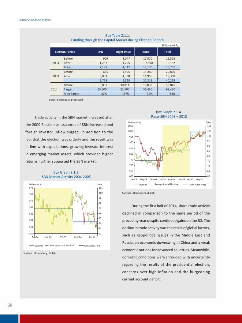
60
Chapter 2. Financial Markets
Trade activity in the SBN market increased after
the 2009 Election as issuances of SBN increased and
foreign investor inflow surged. In addition to the
fact that the election was orderly and the result was
in line with expectations, growing investor interest
in emerging market assets, which provided higher
returns, further supported the SBN market.
During the first half of 2014, share trade activity
declined in comparison to the same period of the
preceding year despite continued gains on the JCI. The
decline in trade activity was the result of global factors,
such as geopolitical issues in the Middle East and
Russia, an economic downswing in China and a weak
economic outlook for advanced countries. Meanwhile,
domestic conditions were shrouded with uncertainty
regarding the results of the presidential election,
concerns over high inflation and the burgeoning
current account deficit.
Box Table 2.1.1.Funding through the Capital Market during Election Periods
Billions of Rp
IPO Right Issue Bond Total
Before 909 3,047 11,570 15,525 After 1,287 1,295 7,600 10,182 Total 2,195 4,342 19,170 25,707 Before 635 4,995 15,260 20,890 After 3,083 4,330 11,955 19,368
3,718 9,325 27,215 40,258 Before 5,001 30,811 18,033 53,845 Target 13,500 22,500 56,430 92,430 % to Target 37% 137% 32% 58%
2014
Election Period
2004
2009
ource: Bloomberg, processed
Sumber : Bloomberg, diolah
Box Graph 2.1.3.SBN Market Activity 2004-2005
Sumber : Bloomberg, diolah
Box Graph 2.1.4.Pasar SBN 2008 – 2010
570
560
550
540
530
520
510
500Feb-04 Jun-04 Oct-04 Feb-050 Jun-05
101
100
99
98
97
96
95
94
93
92
Trillions of Rp Point
Average Annual Nominal IDMA index (RHS)Nominal
1,050
1,000
950
900
850
800
750
700
650
600Jan-08 May-08 Sep-08 Jan-09 May-09 Jan-10 May-10Sep-09
110
105
100
95
90
85
80
75
70
65
60
Trillions of Rp Point
Average Annual Nominal IDMA index (RHS)Nominal

61
Chapter 2. Financial Markets
Source: Bloomberg, processed
Box Graph 2.1.5.Stock Market Activity 2013-Semester I 2014
Source: Bloomberg, processed
Box Graph 2.1.7. JCI Volatility
Source: Bloomberg, processed
Box Graph 2.1.8.SBN Volatility
Source: Bloomberg, processed
Box Graph 2.1.6.SBN Market Activity 2013-Semester I 2014
On the SBN market, a slight drop in the majority
of yields occurred, averaging 17 bps, compared to the
end of 2013. Dissimilar to share trading, SBN trading
expanded as the government continuously issued SBN
from the beginning of the year as part of its front-
loading strategy.
Financial Market Risk during the 2014 Election
During the 2014 Election, risk on the stock market
and SBN market escalated temporarily as JCI volatility
and SBN yield increased. In addition, the increase in
risk was also observed in the yield of SBN auctioned
on the primary market by the government as well as
the coupon rate of corporate bonds. Nevertheless,
the increase in volatility on the stock market and SBN
market was relatively small compared to the period
when concerns arose over the Federal Reserve’s plan
to taper off its monetary policy in the second semester
of 2013 and at the beginning of 2014.
A continued upward JCI trend along with
lower SBN yields also reflected relatively limited
risk despite fluctuations in the wake of a downturn
5500Point Millions
5000
4500
4000
3500
3000
Jan-
13
Feb-
13M
ar-1
3Ap
r-13
May
-13
Jun-
13
Jan-
14
Feb-
14M
ar-1
4Ap
r-14
May
-14
Jun-
14
Jul-1
3
Ags-
13
Sep-
13
Oct
-13
Nov
-13
Dec-
13
14,000
12,000
10,000
8,000
6,000
4,000
2,000
0
Average Annual Volume (millions)JCI Volume (millions) (RHS)
1.500
Trillions of Rp Point
1.400
1.300
1.200
1.100
1.000
900
Jan-13
Mar-13
May-13
Jan-14
Mar-14
May-14
Jul-13
Sep-13
Nov-13
125
120
115
110
105
100
95
90
85
Nominal Trs IDMA Index
JCI (Rebased 1/1/11=100)
Mar
-12
Jun-
12
Sep-
12
Dec
-12
Mar
-13
Jun-
13
Sep-
13
Dec
-13
Mar
-14
Jun-
14
160Point (%)
50
45
40
3530
2520
15
10
50
JCI Volatility (RHS)
140
120
100
80
60
40
20
0
0
5
10
15
20
25
30
35
4(%)
0
Jan-
13Fe
b-13
Mar
-13
Apr-
13
May
-13
Jun-
13Ju
l-13
Aug-
13Se
p-13
Oct
-13
Nov
-13
Dec
-13
Jan-
14Fe
b-14
Mar
-14
Apr-
14M
ay-1
4Ju
n-14
Short Term Medium Term Long Term
Series Maturity Jk Pendek

62
Chapter 2. Financial Markets
during the legislative and presidential elections. The
implementation of an election that was in line with
market expectations bolstered investor confidence
in the increasingly positive economic outlook of
Indonesia.
Positive market perception and optimism were
reflected in the Consensus Forecast published by
Bloomberg regarding several improving domestic
economic indicators. In its Consensus Forecast,
Bloomberg projects inflation to drop to 4.8%, real
GDP at 5.55%, the rupiah at a level of Rp11,775 per
US dollar and the BI rate at 7.5% at the end of 2014.
The improved forecast supports a reduction in risk
on domestic financial markets, thereby prompting an
increase in trade activity.
Source: Bloomberg, processed
Box Graph 2.1.9.JCI, Yield and the Rupiah in 2014
Source: Bloomberg, processed
Box Graph 2.1.10.Actual and Forecasted Indicators
Jun-13Jul-1
3
Ags-13
Sep-13
Oct-13
Nov-13
Dec-13
Jan-14Fe
b-14
Mar-14
Apr-14
May-14
Jun-14
200Point
180
160
140
120
100
80
60
Rebased 1/1/2013
JCI5-year SBN IDR
9 14000
13000
12000
11000
10000
9000
8000
7000
6000
8
7
6
5
4
3
2 2012Q3
2012Q4
2013Q1
2013Q2
2013Q3
2013Q4
2013Q1
2013Q2
2014Q3
2014Q4
(%) (Rp)
BI Rate CPI Real GDP Exchange Rate (RHS)

63
Chapter 2. Financial Markets
Box 2.2 Shadow Banking in Indonesia
Shadow banking has recently come under the
spotlight in the financial systems of a number of
countries. The term ‘shadow banking’ itself was coined
at the G-20 Seoul Summit in 2010 and subsequently
defined by the Financial Stability Board (FSB) as the
system of credit intermediation that involves entities
and activities outside, or in ways only partially linked
to, the traditional system of regulated depository
institutions, with salient parameters including the
transformation of liquidity, maturity and credit risk
along with an element of leverage. Consensus among
all FSB members concerning that definition has not
yet been reached, however it is often referenced in
various publications. Furthermore, several publications
replacethe term shadow banking with non-bank
financial intermediaries (NBFI). Rapid unmonitored,
unregulated and unsupervised growth of shadow
banking was cited as a contributing factor to the
global financial crisis in 2008 in advanced countries,
at least in the United States. Concerns over a re-
escalation of systemic risk from the shadow banking
sector on financial stability re-emerged after the
publication of Basel III regulatory recommendations
for the banking sector that called for space for
regulatory arbitrage between banks and non-banks.
Consequently, G-20 leaders mandated the FSB to
cooperate with international standard setting bodies1
and formulate recommendations to strengthen
monitoring and supervision in order to mitigate system
risk stemming from shadow banking. Discussions and
recommendations remain an ongoing concern at a
number of committees and workstreams coordinated
by the FSB. Bank Indonesia, as a member of the
Financial Stability Board (FSB), continues to follow all
developments.
Fundamentally, shadow banking does not
necessarily have to be limited because in the majority
of developing countries, non-bank intermediation
helps broaden public access to the financial system. In
Indonesia, for instance, the presence of microfinance
institutions is considered crucial in the development
of micro, small and medium enterprises (MSMEs).
Nonetheless, shadow banking regulation and
supervision requires attention in line with its dynamics
within the financial system.
There are two main risk transmission channels
of shadow banking, through interconnectedness
with the banking system as well as direct exposure to
shadow banking by market participants. Regulatory
instruments to control interconnectedness can be
implemented through various methods, for example
by limiting exposure of bank funds and placements
to shadow banking or by expanding capital buffers
for bank exposure to shadow banking. Regulatory
instruments to control exposure to shadow banking
can be introduced directly for non-bank entities
and products in accordance with the nature and
characteristics of the products and entities.
There are numerous types of products and
entities that can be categorised as shadow banking,
particularly in countries with developed financial
markets. One classification approach is based on
similar characteristics, namely: (i) collective investment
contracts with the inherent risk of rush/runs, such
as mutual funds; (ii) funds that generally depend 1) BCBS, IOSCO

64
Chapter 2. Financial Markets
on short-term funding, such as financecompanies;
(iii) market activity intermediation, such as broker-
dealers; (iv) facilitators of credit creation, such as
guarantee companies; and (v) intermediation based
on securitisation trends, such as asset securitisation.
In the context of implementing macroprudential
supervision, Bank Indonesia routinely assesses potential
systemic risk emerging from non-bank financial
institutions. Complementing routine assessments, a
study conducted in 2013 showed that shadow banking
in Indonesia is still at the embryonic stage due to the
relative lack of variation in terms of shadow banking
products, activities and entities compared to practices
in advanced countries. Furthermore, regulation of
shadow banking in Indonesia is considered below
optimal condition with room for improvement for its
supervision. In general, insurers, finance companies,
mutual funds, pension funds and the corporate
sector have been identified as five large entities
with the largest assets. Other additional forms of
shadow banking have also been identified, including
pawnbrokers, venture capital firms and discretionary
funds that also contain transformation risk.
In broader terms, Indonesia has continually
participated in the Global Shadow Banking Monitoring
Exercise since 2012 under the auspices of the Financial
Stability Board (FSB) in order to compare conditions
in Indonesia with those in other countries. Monitoring
on a global scale is not a simple endeavour due to
constraints stemming from the variety of financial
systems, products, activities, data availability and
perceptions of authorities in respondent countries.
In addition to the non-bank financial intermediaries
approach, the FSB also uses the term ‘other financial
intermediaries’ (OFI) as a proxy of shadow banking
size. OFIs consist of NBFI, excluding insurers and
pension funds, namely two industries that are already
relatively well regulated and supervised. Based on
the parameters and survey template issued by the
FSB, relative shadow banking growth in Indonesia
is moderate and decelerating, accounting for a
comparatively small portion of total financial assets.
Source: Financial Stability Board (FSB), processed
Box Graph 2.2.1.Exposure of Non-Bank Financial Intermediaries
Source: Financial Stability Board (FSB), processed
Box Graph 2.2.2.Growth of Non-Bank Financial Intermediaries
0
200
400
600
800
1000
NL UK CH XM HK US KR FR CA ZA DE ES JP BR AU SG IT CL CN MX IN TR ID AR RU SA
Aver
age
Percentage of GDP
Respondent Countries
2011 2012 Bank Assets 2012
-20
-10
0
10
20
30
40
50
CN
AR IN ZA
RU
BR
MX
TR
KR ID US
HK
CA
SG
DE
CH
XM SA JP FR
AU
NL
CL IT
UK
ES
Percentage
2011 2012

65
Chapter 2. Financial Markets
Moving forward, Indonesia faces the challenge
of mitigating risk that emerges from shadow banking
activity, including potential additional complexity
and variation, as well as accurate and up-to-date
information for monitoring purposes. Notwithstanding,
optimism remains concerning additional guidelines
from the FSB and standard setting bodies that
will complement corrective measures in terms of
monitoring, regulation and supervision as well as
inter-authority coordination in Indonesia. In 2015,
the implementation of Act No 1 of 2013, concerning
micro, small and medium enterprises (MSMEs), will
also provide a little more substance to the development
of shadow banking in Indonesia.

This page is intentionally left blank

67
Chapter 3. The Household and Corporate Sectors
The Household and Corporate Sectors
Chapter 3

68
Chapter 3. The Household and Corporate Sectors
69
Chapter 3. The Household and Corporate Sectors
3.1 HOUSEHOLD SECTOR ASSESSMENT
3.1.1 Household Sector Pro le
In general, the performance of the household and corporate sectors improved despite a moderate
slowdown at the outset of the rst semester of as a result of a sluggish global economy, rupiah
deprecia on and soaring in a on Nevertheless, at the end of the rst semester, lower in a on along
with ac vi es associated with the presiden al elec on boosted household and corporate ac vity
ousehold consump on growth underpinned economic e pansion with mi gated ris denoted by low
leverage The gross N ra o of ban credit e tended to households was also rela vely low despite a
slight increase on the preceding semester oten al ris s that demanded a en on in the household
sector were found to a ect low income households with high leverage and no savings omes c
demand pic ed up in the corporate sector as a result of elec on ac vity as well as prepara ons for
the holy fas ng month of amadan, have s mulated business ac vity oo ing ahead, the corporate
sector will con nue to face poten al ris s emana ng from persistently wea prices of leading non
oil gas e port commodi es
The Household and Corporate SectorsChapter3
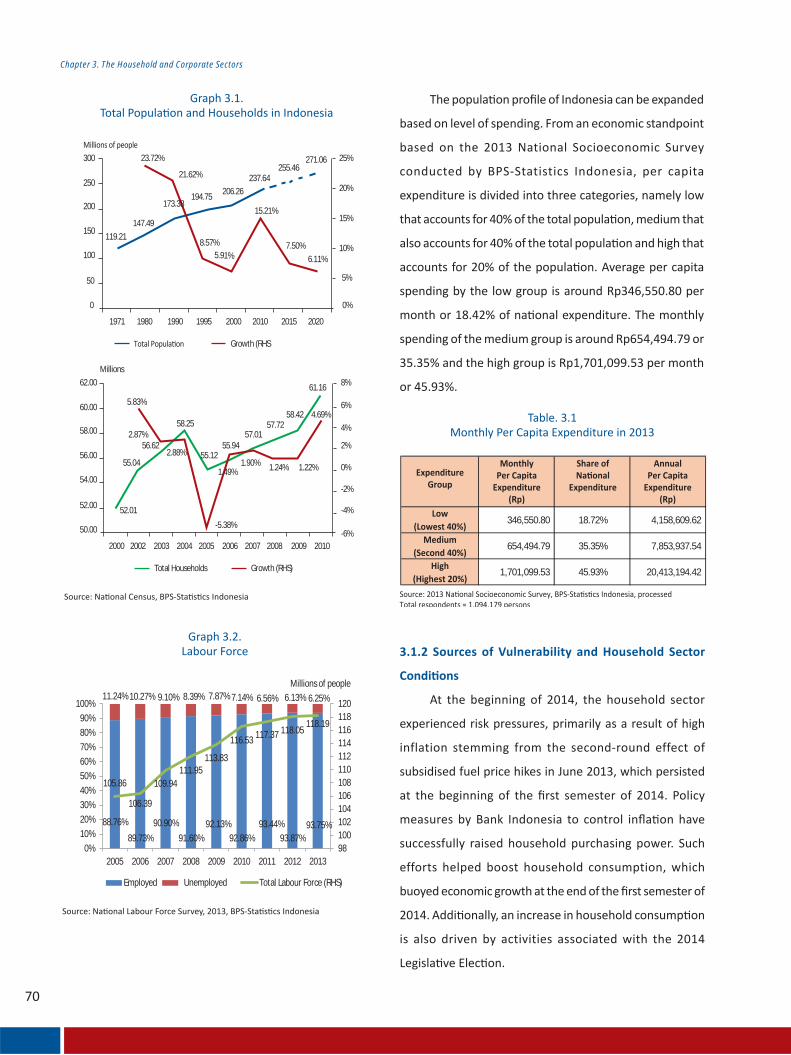
Chapter 3. The Household and Corporate Sectors
346,550.80 18.72% 4,158,609.62
654,494.79 35.35% 7,853,937.54
1,701,099.53 45.93% 20,413,194.42
Low(Lowest 40%)
Medium(Second 40%)
High(Highest 20%)
ExpenditureGroup
MonthlyPer Capita
Expenditure(Rp)
Share ofNa onal
Expenditure
AnnualPer Capita
Expenditure(Rp)
3.1.2 Sources of Vulnerability and Household Sector
Condi ons
1971
119.21
147.49
173.38194.75
206.26
237.64255.46
271.06
5.91%8.57%
21.62%
23.72% 25%
20%
15%
10%
5%
0%
300
250
200
150
100
50
0
6.11%
15.21%
7.50%
19901980 1995 2000 2010 2015 2020
Growth (RHS
Total Households
8%
6%
4%
-6%
2%
-4%
0%
-2%
62.00
Millions
60.00
58.00
56.00
54.00
52.00
50.00
2000
52.01
55.04
56.62
58.25
55.1255.94
57.0157.72
58.42
61.16
5.83%
2.87%
2.88%
-5.38%
1.49%1.90% 1.24% 1.22%
4.69%
201020092008200720062005200420032002
Growth (RHS)
88.76%
89.73%
90.90%
91.60%92.13%
92.86%93.44%
93.87%93.75%
11.24% 10.27% 9.10% 8.39% 7.87% 7.14% 6.56% 6.13% 6.25%
105.86
106.39
109.94111.95
113.83
116.53 117.37 118.05118.19
98100102104106108110112114116118120
0%
10%
20%
30%
40%
50%
60%
70%
80%
90%
100%
2005 2006 2007 2008 2009 2010 2011 2012 2013
Millions of people
Employed Unemployed Total Labour Force (RHS)
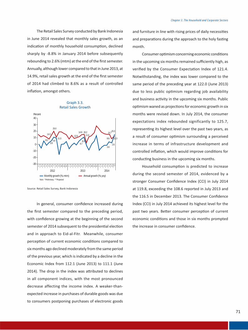
Chapter 3. The Household and Corporate Sectors
2012
Monthly growth (%, mtm)Note: *Preliminary; **Projected
20.0
14.3
8.011.3
14.9 14.715.3
12.38.6
3.62.6
12.0
15.211.6
4.78.3
2.85.6
Annual growth (%, yoy)
40Percent
30
20
10
-10
-20
-30
0
1 2 3 4 5 6 7 8 9 10 11 12 1 2 3 4 5 6 7 8 9 10 11 12 1 2 3 4 5 6 7**
2013 2014
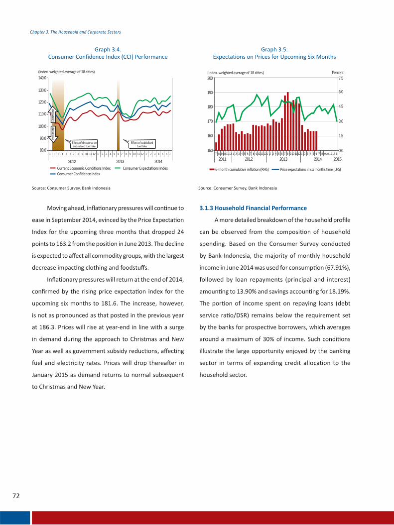
Chapter 3. The Household and Corporate Sectors
200 7.5
6.0
4.5
3.0
0.0
1.5
190
180
170
160
1501 2 3 4 5 6 7 8 9 10 11 127 8 9 10 11 12 1 2 3 4 5 6 7 8 9 10 11 12 1 2 3 4 5 6 7 8 9 10 11 12 1
2011 2012 2013 2014 2015
Percent
3.1.3 Household Financial Performance
2012
140.0
130.0
120.0
110.0
100.0
90.0
80.01 2 3 4 5 6 7 8 9 10 11 12 1 2 3 4 5 6 7 8 9 10 11 12 1 2 3 4 5 6 7
2013 2014

Chapter 3. The Household and Corporate Sectors
Income Rp 1.22-2.45 juta Rp 2.56-3.65 juta Rp 3.76-4.85 juta Rp 5.03- 6.26 juta > Rp 6.26 juta Average
70.3% 69.3% 68.5% 66.9% 64.3% 67.9%
Loanrepayments
11.6% 12.9% 14.0% 14.6% 15.6% 13.9%
Savings 18.1% 17.8% 17.5% 18.5% 20.1% 18.2%Total 100.0% 100.0% 100.0% 100.0% 100.0% 100.0%
Source: Consumer Survey. Bank Indonesia
0-10% 10%-20% 20%-30% >30%
Rp 1.22-2.45 juta 27.97% 17.38% 5.03% 3.44% 2.11%
Rp 2.56-3.65 juta 34.67% 19.64% 7.85% 4.69% 2.48%Rp 3.76-4.85 juta 20.81% 11.37% 4.73% 3.27% 1.44%Rp 5.03- 6.26 juta 8.64% 4.49% 2.03% 1.38% 0.74%
> Rp 6.26 juta 7.91% 4.02% 1.57% 1.35% 0.98%Total 100.00% 56.90% 21.21% 14.13% 7.75%
IncomeDSR
Total
Source: Consumer Survey, Bank Indonesia

Chapter 3. The Household and Corporate Sectors
Source: Consumer Survey. Bank Indonesia
c
0-10% 10%-20% 20%-30% >30% Inabilityto save
Rp 1.22-2.45 juta 27.97% 6.54% 5.94% 4.42% 4.37% 6.70%
Rp 2.56-3.65 juta 34.67% 9.96% 9.45% 5.67% 4.20% 5.38%Rp 3.76-4.85 juta 20.81% 7.71% 5.82% 3.30% 2.00% 1.99%Rp 5.03- 6.26 juta 8.64% 2.95% 2.58% 1.27% 1.03% 0.82%
> Rp 6.26 juta 7.91% 2.36% 2.44% 1.44% 1.03% 0.66%Total 100.00% 29.51% 26.23% 16.10% 12.62% 15.54%
IncomeSaving
TotalPercent
Property
100
2010
76.72 74.48 79.01 78.47
17.54 16.91 14.10 15.88
5.74 8.61 6.89 5.65
2011 2012 2013
90
80
70
60
50
40
30
20
10
0
Others (motor vehicles. householdequipment and clothing)
Financial Assets
Household Assets
PercentHousehold Financial Assets
Savings held at bank
100
2010
49.81 49.30 50.30 55.29
35.67 40.98 42.76 29.23
10.60 7.01
0.35 2.272.713.92
13.206.59
2011 2012 2013
90
80
70
60
50
40
30
20
10
0
Savings held at non bankInvestment Others (business and non-business receivables)

Chapter 3. The Household and Corporate Sectors
3.1.4 Bank Exposure to the Household Sector
19.5317.98
18.93
15.54
3.783.04 2.12 2.58
15.75 14.9516.80
12.9613.09 12.3813.46
9.97
0
5
10
15
20
25
2010 2011 2012 2013
Percent
Total debt/income Short-term debt/income
Long-term debt/income Bank debt/income
45.07%
15.25%
0.22%
34.80%
4.67%
43.64%
15.22%
0.22%
37.15%
3.77%
2014
2013
Percent
3.61
3.30
3.33
2.62
4.06
3.81
3.71
2.96
2.00
2.50
3.00
3.50
4.00
4.50
2010 2011 2012 2013
Total debt/total assets
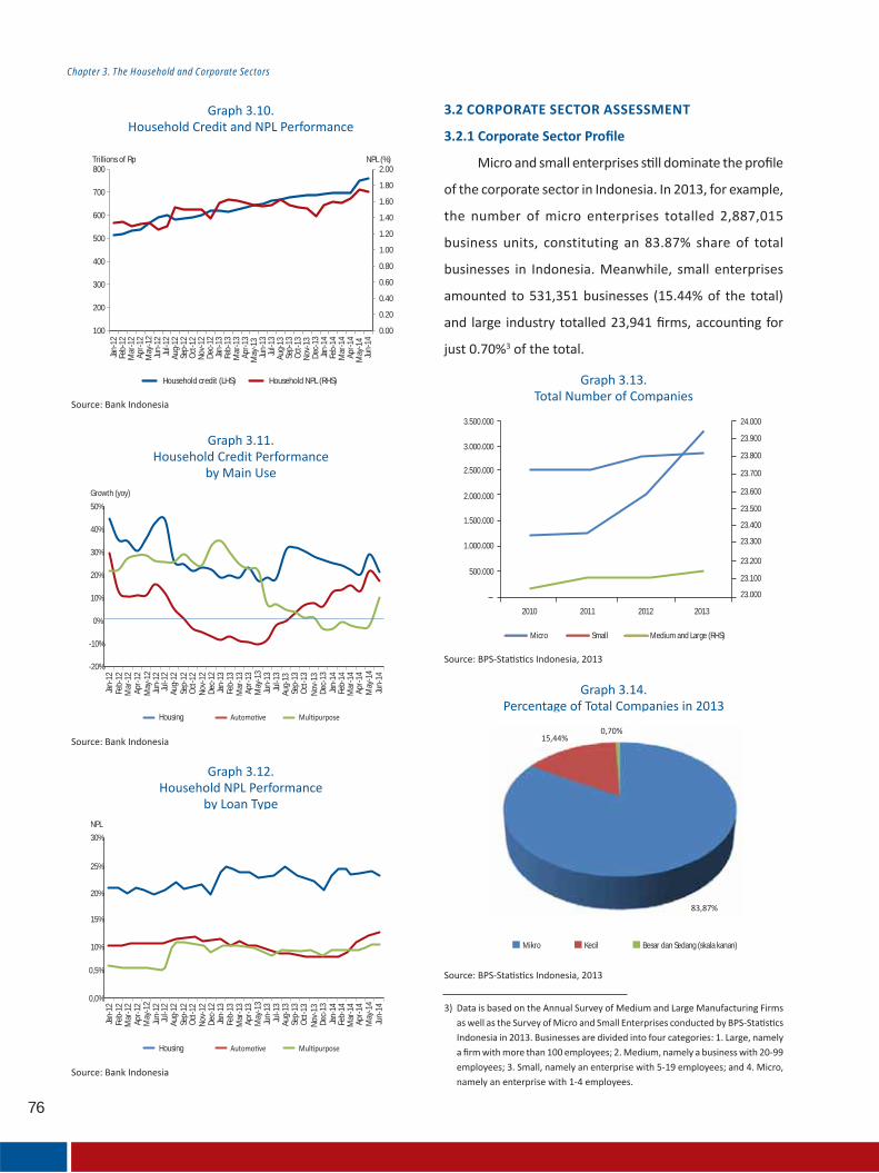
76
Chapter 3. The Household and Corporate Sectors
3.2 CORPORATE SECTOR ASSESSMENT
3.2.1 Corporate Sector Pro le
0.00
0.20
0.40
0.60
0.80
1.00
1.20
1.40
1.60
1.80
2.00
100
200
300
400
500
600
700
800
Jan-
12Fe
b-12
Mar
-12
Apr-
12M
ay-1
2Ju
n-12
Jul-1
2Au
g-12
Sep-
12O
ct-1
2N
ov-1
2De
c-12
Jan-
13Fe
b-13
Mar
-13
Apr-
13M
ay-1
3Ju
n-13
Jul-1
3Au
g-13
Sep-
13O
ct-1
3N
ov-1
3De
c-13
Jan-
14Fe
b-14
Mar
-14
Apr-
14M
ay-1
4Ju
n-14
NPL (%)Trillions of Rp
Household credit (LHS) Household NPL (RHS)
Jan-
12Fe
b-12
Mar
-12
Apr-
12M
ay-1
2Ju
n-12
Jul-1
2Au
g-12
Sep-
12O
ct-1
2N
ov-1
2De
c-12
Jan-
13Fe
b-13
Mar
-13
Apr-
13M
ay-1
3Ju
n-13
Jul-1
3Au
g-13
Sep-
13O
ct-1
3N
ov-1
3De
c-13
Jan-
14Fe
b-14
Mar
-14
Apr-
14M
ay-1
4Ju
n-14
-20%
-10%
0%
10%
20%
30%
40%
50%
Growth (yoy)
Housing
3.500.000
2010
Micro
2011 2012 2013
3.000.000
2.500.000
2.000.000
1.500.000
1.000.000
500.000
24.000
23.900
23.800
23.700
23.600
23.500
23.400
23.300
23.200
23.100
23.000
Small Medium and Large (RHS)
Jan-
12Fe
b-12
Mar
-12
Apr-
12M
ay-1
2Ju
n-12
Jul-1
2Au
g-12
Sep-
12O
ct-1
2N
ov-1
2De
c-12
Jan-
13Fe
b-13
Mar
-13
Apr-
13M
ay-1
3Ju
n-13
Jul-1
3Au
g-13
Sep-
13O
ct-1
3N
ov-1
3De
c-13
Jan-
14Fe
b-14
Mar
-14
Apr-
14M
ay-1
4Ju
n-14
0,0%
0,5%
10%
15%
20%
25%
30%
NPL
Housing
Mikro Kecil Besar dan Sedang (skala kanan)

77
Chapter 3. The Household and Corporate Sectors
3.2.2 Sources of Vulnerability in the Corporate Sector
16.000USD
14.000
12.000
10.000
8.000
6.000
4.000
2.000
Natural Gas (LHS) Crude Oil (RHS) Coal (RHS)
2007
Q1 Q2 Q3 Q420
08Q1 Q2 Q3 Q4
2009
Q1 Q2 Q3 Q420
10Q1 Q2 Q3 Q4
2011
Q1 Q2 Q3 Q420
12Q1 Q2 Q3 Q4
2013
Q1 Q2 Q3 Q420
14Q1 Q2
0
160USD
105,37USD/Barrel
60,05USD/Short Ton
4.461USD/MBTU
140
120
100
80
60
40
20
0
7.000USD
6.000
5.000
4.000
3.000
2.000
1.000
Rubber CPO (RHS)
2007
Q1 Q2 Q3 Q420
08Q1 Q2 Q3 Q4
2009
Q1 Q2 Q3 Q420
10Q1 Q2 Q3 Q4
2011
Q1 Q2 Q3 Q420
12Q1 Q2 Q3 Q4
2013
Q1 Q2 Q3 Q420
14Q1 Q2
1.400
1.200
1.000
800
600
400
200
USD
774,24USD/Metric Ton
2.330USD/Metric Ton
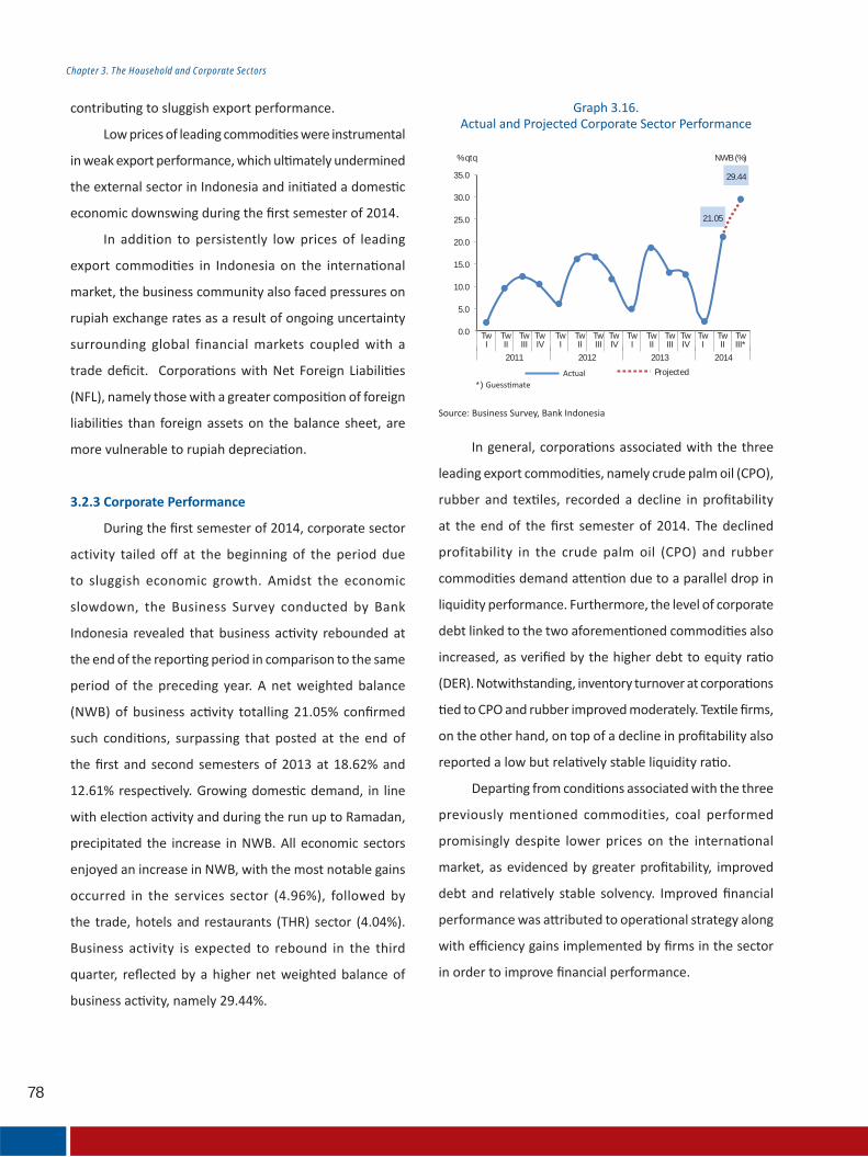
78
Chapter 3. The Household and Corporate Sectors
3.2.3 Corporate Performance
21.05
29.44
0.0
5.0
10.0
15.0
20.0
25.0
30.0
35.0
TwII
TwI
TwIII*
TwII
TwI
TwIII
TwIV
TwII
TwI
TwIII
TwIV
TwII
TwI
TwIII
TwIV
2011 2012 2013 2014
% qtq NWB (%)
*)
Projected
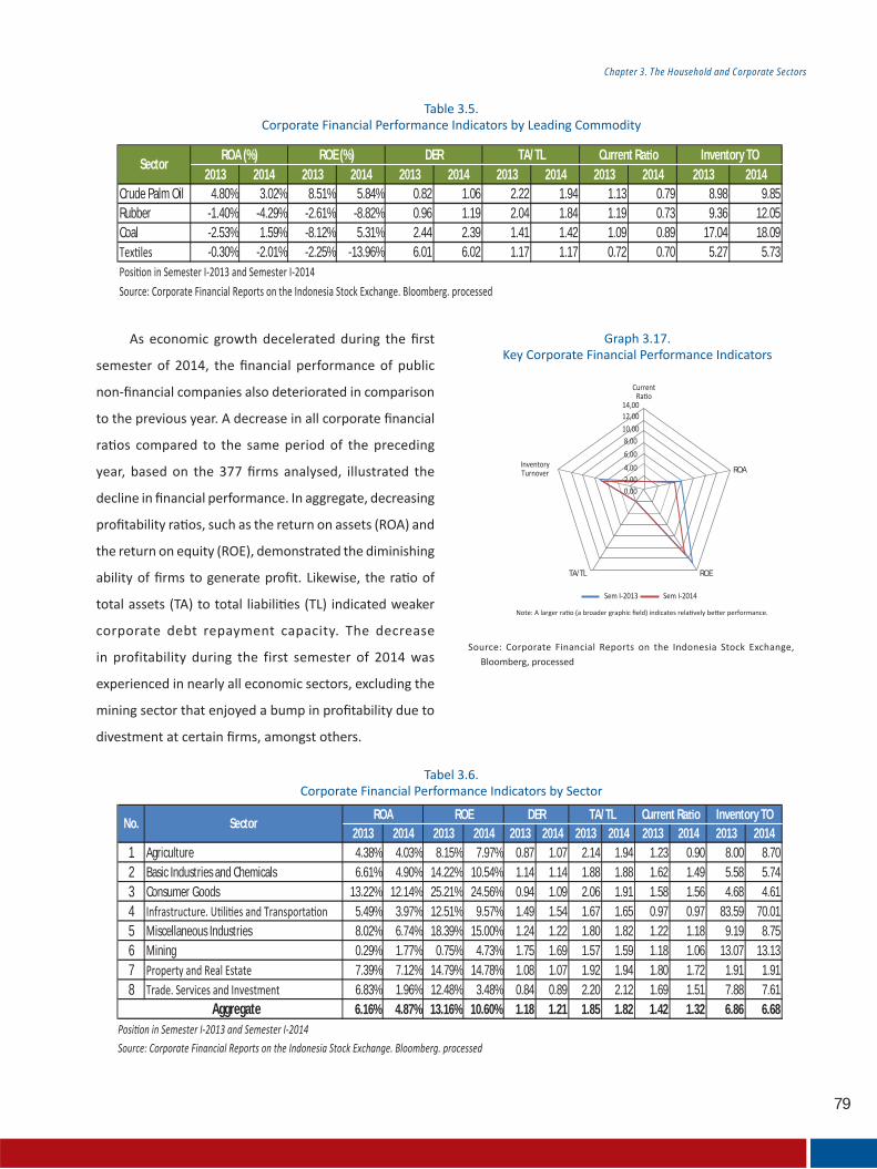
79
Chapter 3. The Household and Corporate Sectors
2013 2014 2013 2014 2013 2014 2013 2014 2013 2014 2013 2014Crude Palm Oil 4.80% 3.02% 8.51% 5.84% 0.82 1.06 2.22 1.94 1.13 0.79 8.98 9.85Rubber -1.40% -4.29% -2.61% -8.82% 0.96 1.19 2.04 1.84 1.19 0.73 9.36 12.05Coal -2.53% 1.59% -8.12% 5.31% 2.44 2.39 1.41 1.42 1.09 0.89 17.04 18.09
-0.30% -2.01% -2.25% -13.96% 6.01 6.02 1.17 1.17 0.72 0.70 5.27 5.73
Inventory TOSector
ROA (%) ROE (%) DER TA/TL Current Ra o
2013 2014 2013 2014 2013 2014 2013 2014 2013 2014 2013 20141 Agriculture 4.38% 4.03% 8.15% 7.97% 0.87 1.07 2.14 1.94 1.23 0.90 8.00 8.702 Basic Industries and Chemicals 6.61% 4.90% 14.22% 10.54% 1.14 1.14 1.88 1.88 1.62 1.49 5.58 5.743 Consumer Goods 13.22% 12.14% 25.21% 24.56% 0.94 1.09 2.06 1.91 1.58 1.56 4.68 4.614 5.49% 3.97% 12.51% 9.57% 1.49 1.54 1.67 1.65 0.97 0.97 83.59 70.015 Miscellaneous Industries 8.02% 6.74% 18.39% 15.00% 1.24 1.22 1.80 1.82 1.22 1.18 9.19 8.756 Mining 0.29% 1.77% 0.75% 4.73% 1.75 1.69 1.57 1.59 1.18 1.06 13.07 13.137 7.39% 7.12% 14.79% 14.78% 1.08 1.07 1.92 1.94 1.80 1.72 1.91 1.918 6.83% 1.96% 12.48% 3.48% 0.84 0.89 2.20 2.12 1.69 1.51 7.88 7.61
6.16% 4.87% 13.16% 10.60% 1.18 1.21 1.85 1.82 1.42 1.32 6.86 6.68Aggregate
TA/TL Current Ra o Inventory TONo. Sector
ROA ROE DER
ROA
ROETA/TL
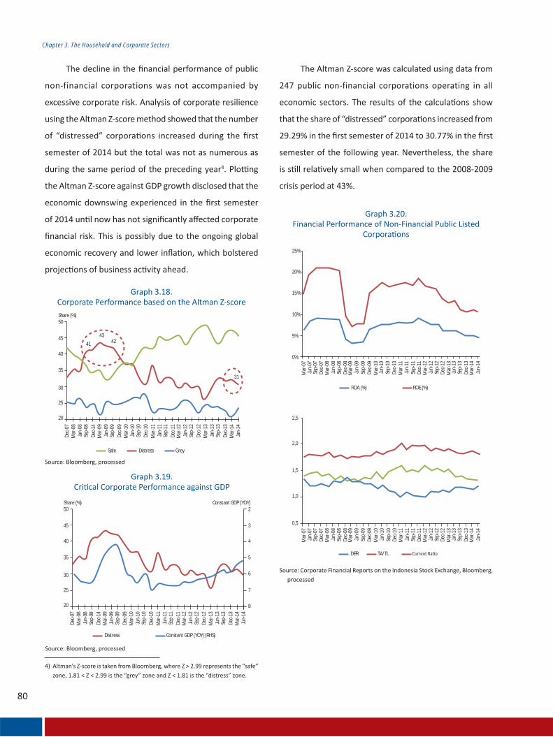
Chapter 3. The Household and Corporate Sectors
50Share (%) Constant GDP (YOY)
2
3
4
5
6
7
8
Distress Constant GDP (YOY) (RHS)
Dec-
07M
ar-0
8Ju
n-08
Sep-
08De
c-14
Mar
-09
Jun-
09Se
p-09
Dec-
09M
ar-1
0Ju
n-10
Sep-
10De
c-10
Mar
-11
Jun-
11Se
p-11
Dec-
11M
ar-1
2Ju
n-12
Sep-
12De
c-12
Mar
-13
Jun-
13Se
p-13
Dec-
13M
ar-1
4Ju
n-14
45
40
35
30
25
20
50Share (%)
41
43
31
42
DistressSafe Grey
Dec-
07M
ar-0
8Ju
n-08
Sep-
08De
c-14
Mar
-09
Jun-
09Se
p-09
Dec-
09M
ar-1
0Ju
n-10
Sep-
10De
c-10
Mar
-11
Jun-
11Se
p-11
Dec-
11M
ar-1
2Ju
n-12
Sep-
12De
c-12
Mar
-13
Jun-
13Se
p-13
Dec-
13M
ar-1
4Ju
n-14
45
40
35
30
25
20
ROA (%) ROE (%)
25%
20%
15%
10%
5%
0%
Mar
-07
Jun-
07Se
p-07
Dec-
07M
ar-0
8Ju
n-08
Sep-
08De
c-08
Mar
-09
Jun-
09Se
p-09
Dec-
09M
ar-1
0Ju
n-10
Sep-
10De
c-10
Mar
-11
Jun-
11Se
p-11
Dec-
11M
ar-1
2Ju
n-12
Sep-
12De
c-12
Mar
-13
Jun-
13Se
p-13
Dec-
13M
ar-1
4Ju
n-14
DER TA/TL
2,5
2,0
1,5
1,0
0,5
Mar
-07
Jun-
07Se
p-07
Dec-
07M
ar-0
8Ju
n-08
Sep-
08De
c-08
Mar
-09
Jun-
09Se
p-09
Dec-
09M
ar-1
0Ju
n-10
Sep-
10De
c-10
Mar
-11
Jun-
11Se
p-11
Dec-
11M
ar-1
2Ju
n-12
Sep-
12De
c-12
Mar
-13
Jun-
13Se
p-13
Dec-
13M
ar-1
4Ju
n-14

Chapter 3. The Household and Corporate Sectors
Buku 1 Buku 2 Buku 3 Buku 4
Mar Jun
2010
50.00%
45.00%
40.00%
35.00%
30.00%
25.00%
20.00%
15.00%
10.00%
5.00%
0.00%
2011 2012 2013 2014
Sep Dec Mar Jun Sep Dec Mar Jun Sep Dec Mar Jun Sep Dec Mar Jun
Corporate
Mar Jun
2010
100.00%
90.00%
80.00%
70.00%
60.00%
50.00%
40.00%
30.00%
20.00%
10.00%
0.00%
2011 2012 2013 2014
Sep Dec Mar Jun Sep Dec Mar Jun Sep Dec Mar Jun Sep Dec Mar Jun
Households and Individual Others
3.2.4 Bank Exposure to the Corporate Sector
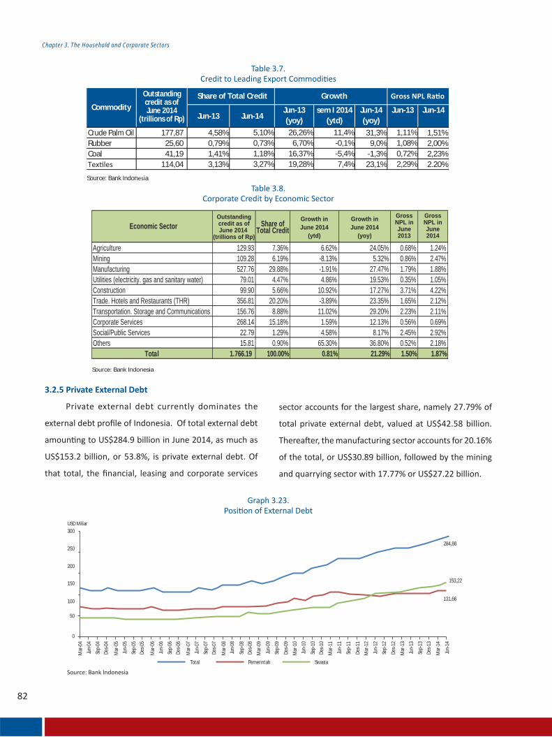
Chapter 3. The Household and Corporate Sectors
300USD Miliar
Total
284,88
153,22
131,66
250
200
150
100
50
0
Mar
-07
Jun-
07
Sep-
07
Des-
07
Mar
-06
Jun-
06
Sep-
06
Des-
06
Mar
-05
Jun-
05
Sep-
05
Des-
05
Mar
-04
Jun-
04
Sep-
04
Des-
04
Mar
-08
Jun-
08
Sep-
08
Des-
08
Mar
-09
Jun-
09
Sep-
09
Des-
09
Mar
-10
Jun-
10
Sep-
10
Des-
10
Mar
-11
Jun-
11
Sep-
11
Des-
11
Mar
-12
Jun-
12
Sep-
12
Des-
12
Mar
-13
Jun-
13
Sep-
13
Des-
13
Mar
-14
Jun-
14
Pemerintah Swasta
3.2.5 Private External Debt
Jun-13 Jun-14Jun-13 (yoy)
sem I 2014 (ytd)
Jun-14 (yoy)
Jun-13 Jun-14
Crude Palm Oil 177,87 4,58% 5,10% 26,26% 11,4% 31,3% 1,11% 1,51%Rubber 25,60 0,79% 0,73% 6,70% -0,1% 9,0% 1,08% 2,00%Coal 41,19 1,41% 1,18% 16,37% -5,4% -1,3% 0,72% 2,23%
114,04 3,13% 3,27% 19,28% 7,4% 23,1% 2,29% 2.20%
Commodity
Outstandingcredit as ofJune 2014
(trillions of Rp)
Share of Total Credit Growth
Source: Bank Indon ia
Outstandingcredit as ofJune 2014
(trillions of Rp)
Growth inJune 2014
(ytd)
Growth inJune 2014
(yoy)
GrossNPL inJune2013
GrossNPL inJune2014
Agriculture 129.93 7.36% 6.62% 24.05% 0.68% 1.24%Mining 109.28 6.19% -8.13% 5.32% 0.86% 2.47%Manufacturing 527.76 29.88% -1.91% 27.47% 1.79% 1.88%Utilities (electricity. gas and sanitary water) 79.01 4.47% 4.86% 19.53% 0.35% 1.05%Construction 99.90 5.66% 10.92% 17.27% 3.71% 4.22%Trade. Hotels and Restaurants (THR) 356.81 20.20% -3.89% 23.35% 1.65% 2.12%Transportation. Storage and Communications 156.76 8.88% 11.02% 29.20% 2.23% 2.11%Corporate Services 268.14 15.18% 1.59% 12.13% 0.56% 0.69%Social/Public Services 22.79 1.29% 4.58% 8.17% 2.45% 2.92%Others 15.81 0.90% 65.30% 36.80% 0.52% 2.18%
Total 1.766.19 100.00% 0.81% 21.29% 1.50% 1.87%
Share ofTotal CreditEconomic Sector
Source: Bank Indonesia

Chapter 3. The Household and Corporate Sectors
6
7
(Million of USD)
2014
Sem I Sem II Sem I1 Agriculture, Livestock, Fisheries and Forestry 4,063 4,637 4,969 5,744 6,454 7,414 7,720 5.04%
2 Mining and Quarrying 12,103 10,842 16,878 20,346 25,240 26,381 27,224 17.77%
3 Manufacturing 19,336 19,471 22,646 25,637 26,660 29,168 30,885 20.16%4 9,707 13,142 14,946 16,855 16,456 17,088 18,734 12.23%
5 291 320 755 667 661 968 1,010 0.66%6 3,744 3,157 4,919 6,565 6,787 7,632 8,185 5.34%
7 4,739 6,272 8,108 10,080 10,326 10,084 10,479 6.84%8 Financial, Leasing and Corporate Services 15,981 21,048 28,390 34,862 35,706 37,180 42,579 27.79%
9 Services 400 769 584 637 563 975 965 0.63%
10 Others 3,242 4,130 4,537 4,852 5,135 5,150 5,443 3.55%
TOTAL 73,606 83,789 106,732 126,245 133,988 142,041 153,224 100.00%
ShareSem I 2014
No Economic Sector 20122013
2009 2010 2011

Chapter 3. The Household and Corporate Sectors
(million of USD)
Sem I Sem II Sem I*
1, Parent Company 7,547 11,947 15,785 21,677 23,128 25,867 69.73%
Agriculture, Livestock, Fisheries and Forestry 703 1,044 992 1,826 2,763 2,735 7.37%Mining and Quarrying 887 1,190 1,368 2,718 2,061 2,716 7.32%Manufacturing 3,376 3,871 5,912 8,215 8,500 9,495 25.60%
409 827 899 826 1,892 1,928 5.20%155 204 332 175 391 368 0.99%588 788 1,234 1,428 1,262 1,731 4.67%486 2,496 3,046 4,293 4,072 4,320 11.64%
Financial, Leasing and Corporate Services 649 1,225 1,740 1,918 1,622 1,841 4.96%Services 133 127 43 39 37 38 0.10%Others
Agriculture, Livestock, Fisheries and ForestryMining and QuarryingManufacturing
Financial, Leasing and Corporate ServicesServicesOthers
160 174 221 239 528 694 1.87%2, 10,956 10,392 11,491 10,915 11,275 11,231 30.27%
211 163 - - 33 34 0.09%2,994 2,364 3,952 3,205 3,230 3,108 8.38%1,429 1,493 1,356 927 1,056 1,083 2.92%4,143 4,404 3,840 4,023 4,017 4,022 10.84%
- - 93 1 - - 0.00%928 157 546 740 737 745 2.01%712 1,053 1,160 1,187 1,187 1,192 3.21%433 242 188 458 823 854 2.30%
55 220 167 167 - - 0.00%52 295 189 206 193 193 0.52%
18,503 22,339 27,276 32,592 34,402 37,098 100.00%TOTAL (1+2)
Share ofSem I 2014
2009 2010No Economic Sector 20112013 2014

Chapter 3. The Household and Corporate Sectors
Box 3.1 Credit Risk Concentra on in the Corporate Sector
Share of Debtors

86
Chapter 3. The Household and Corporate Sectors
Box 3.2 Risk of increasing Nonbank Private External Debt
8
9
Creditor Status
Short
Stress Testof Bank Credit
Export
Domes c
PeriodLong
Corporate

87
Chapter 3. The Household and Corporate Sectors
Throughout2013
( USD ( USD
N t Supp y/
Short Domes c 662 102,895 7,353 (36,942) Export 177 37,278 3,593 1,397
Short-Term Total 839 140,173 10,947 (35,546
BorrowerStatus
A 19 7,319 34%Non A 94 13,940 66%Tot 113 21,259 100%
StatusTotal Total
US ) US )Share(%)
Share(%)
113 21,259 18%2,051 95,407 82%
Tot 2,164 116,666 100%
-0,2
0,3
0,8
1,3
1,8
2,3
2,8
3,3
-12,0%
-7,0%
-2,0%
3,0%
8,0%
13,0%
18,0%
23,0%
28,0%
Mar-0
8…
Des-0
8
Sep-0
9
Jun-10
Mar-1
1
Des-1
1
Sep-1
2
Jun-13
Jun-08
Mar-0
9
Des-0
9
Sep-1
0
Jun-11
Mar-1
2
Dec-1
2
Sep-1
3
Sep-0
8
Jun-09
Mar-1
0
Des-1
0
Sep-1
1
Jun-12
Mar-1
3
Mar-0
8…
Des-0
8
Sep-0
9
Jun-10
Mar-1
1
Des-1
1
Sep-1
2
Jun-13
Non A as
Non A as
Non A as
Non A as
A asA as
A as
A as
ROA DER (rhs) Current Ra o (rhs)

88
Chapter 3. The Household and Corporate Sectors
Safe
SectorGrey Safe Grey Safe Grey Safe Grey
Share (%)

89
The Banking Industry andNon-bank Financial Ins tu ons
Chapter 4

90

91
4.1 THE BANKING SECTOR
4.1.1 An Assessment of Liquidity and Risk
Against a backdrop of moderating economic growth, widespread uncertainty concerning the
presiden al elec on as well as ght macroeconomic policy, the banking sector, which dominates the
nancial system of Indonesia, con nued to improve with rela vely maintained levels of resilience
and risk uch condi ons were re ected by preserved liquidity and mi gated liquidity risk, improved
intermedia on performance with funding risk and credit risk maintained at safe levels despite a slight
escala on as well as mi gated market risk uring the repor ng semester, with the support of a solid
capital base, banks successfully increased pro tability Greater pro tability, coupled with liquid asset
growth and slower credit growth, evidenced greater bank prudence in an cipa on of poten al risk
The results of stress tests revealed that the Capital Adequacy a o CA of the banking industry is
su cient to an cipate shocks as well as moun ng poten al credit and market risks
Chapter4
The Banking Industry andNon-bank Financial Ins tu ons
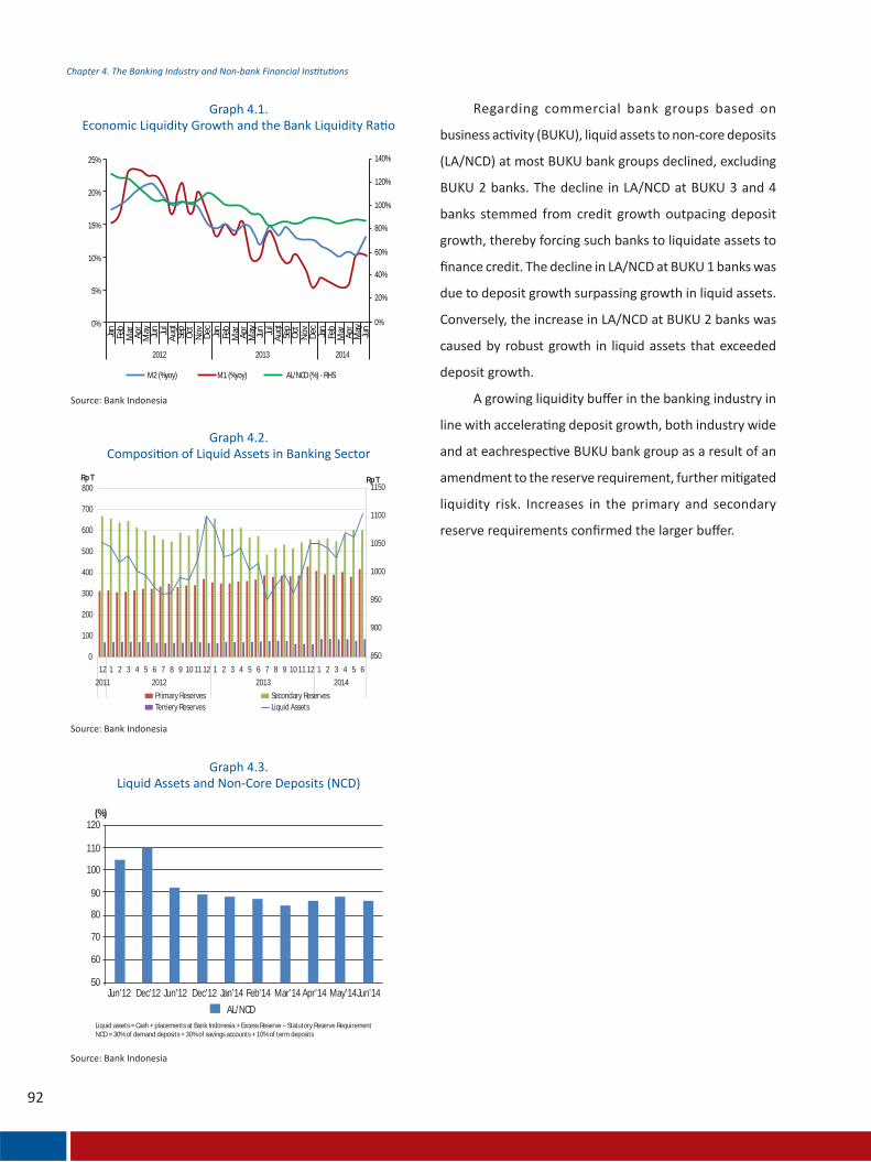
25% 140%
120%
100%
80%
60%
40%
20%
0%
20%
15%
10%
5%
2012 2013 2014
0%
Jan
Feb
Mar
Apr
May Jun Jul
Augt
Sep
Oct
Nov Dec Jan
Feb
Mar
Apr
May Jun Jul
Augt
Sep
Oct
Nov Dec Jan
Feb
Mar
Apr
May
Jun
M2 (%yoy) M1 (%yoy) AL/NCD (%) - RHS
850
900
950
1000
1050
1100
1150
0
100
200
300
400
500
600
700
800
12 1 2 3 4 5 6 7 8 9 10 11 12 1 2 3 4 5 6 7 8 9 10 11 12 1 2 3 4 5 6
2011 2012 2013 2014
Rp TRp T
Primary Reserves Secondary ReservesTer ery Reserves Liquid Assets
(%)
AL/NCD
Jun’12 Dec’12 Jun’12 Dec’12 Jun’14Jan’14 Feb’14 Mar’14 Apr’14 May’14
120
Liquid assets = Cash + placements at Bank Indonesia + Excess Reserve – Statutory Reserve RequirementNCD = 30% of demand deposits + 30% of savings accounts + 10% of term deposits
110
100
90
80
70
60
50

eposit erformance and isk4.1.2 An Assessment of Intermedia on and Risk
Sem II-2012 Sem I-2013 Sem II-2013 Sem I-2014
Credit (Rp T) 145.32 160.20 178.36 193.59Deposits (RP T) 171.32 197.92 196.45 233.23LDR (%) 84.82 80.94 90.79 83.01
Credit (Rp T) 699.44 771.02 871.79 924.04Deposits (RP T) 742.90 818.16 832.29 916.07LDR (%) 94.15 94.24 104.75 100.87
Credit (Rp T) 731.31 775.28 852.86 904.79Deposits (RP T) 820.13 836.03 958.89 970.11LDR (%) 89.17 92.73 88.94 93.27
Credit (Rp T) 1,131.80 1,252.62 1,389.86 1,445.75Deposits (RP T) 1,490.85 1,522.31 1,676.34 1,715.10LDR (%) 75.92 82.28 82.91 84.30
Credit (Rp T) 2,707.86 2,959.12 3,292.87 3,468.16Deposits (RP T) 3,225.20 3,374.42 3,663.97 3,834.50LDR (%) 83.96 87.69 89.87 90.45
BUKU 1
BUKU 2
BUKU 3
BUKU 4
Industri
Primary (%) 62.24 62.31 62.52 63.15 62.95 55.76 56.14Secondary (%) 19.45 19.47 19.54 19.73 19.67 27.88 28.07LDR (%) 4.90 3.87 3.42 2.38 1.71 0.76 0.48Foreign Exchange (%) 13.42 14.34 14.53 14.74 15.67 15.61 15.31Total GWM (%) 100.00 100.00 100.00 100.00 100.00 100.00 100.00
Statutory ReserveRequirement Sem I - 2011 Sem II - 2011 Sem I - 2012 Sem II - 2012 Sem I - 2013 Sem II - 2013 Sem I - 2014
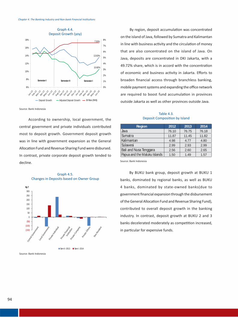
Region 2012 2013 2014Java 76.10 76.75 76.18Sumatra 11.87 11.45 11.82Kalimantan 4.98 4.77 4.80Sulawesi 2.99 2.93 2.99Bali and Nusa Tenggara 2.56 2.60 2.65Papua and the Maluku Islands 1.50 1.49 1.57
13.63%
10.60%
7.50%
0%
1%
2%
3%
4%
5%
6%
7%
8%
6%
8%
10%
12%
14%
16%
18%
Semester I Semester II Semester I
BI Rate (RHS)Adjusted Deposit GrowthDeposit Growth
(150)
(100)
(50)
0
50
100
150
200
250
300
Rp T
Sem II -2013 Sem I -2014
Centra
l Gov
ernm
ent
Loca
l Gov
ernm
ent
Priva
te-In
dividua
lPr
ivate
-Fina
ncial
Insti
tutio
nPr
ivate
-Com
pany
Priva
te-O
ther
s
Non-R
esiden
t

Market Share inSemester I 2014 (%)
BUKU 1 28.76 20.81 17.54 14.67 17.84 6.08BUKU 2 22.22 15.06 13.39 12.03 11.97 23.89BUKU 3 21.16 17.71 12.55 16.92 16.04 25.30BUKU 4 19.87 14.62 15.06 12.44 12.66 44.73Industry 21.24 15.81 14.16 13.60 13.63 100.00
Sem I 2014Deposits Growth (%) Sem I 2012 Sem II 2012 Sem I 2013 Sem II 2013
Industry(Rp T)
Sem I2012
Sem II2012
Sem I2013
Sem II2013
Sem I2014
Demand Deposits 718.26 767.07 827.40 846.78 911.98
Saving 939.20 1,076.83 1,066.01 1,212.71 1,167.02
Term Deposits 1,298.37 1,381.30 1,481.02 1,604.48 1,755.50
Total Deposits 2,955.83 3,225.20 3,374.42 3,663.97 3,834.50
0%
10%
20%
30%
40%
50%
60%
70%
80%
90%
100%
Smt I 2010 Smt II 2010 Smt I 2011 Smt II 2011 Smt I 2012 Smt II 2012 Smt I 2013 Smt II 2013 Smt I 2014
Demand deposits Savings Term deposits <= 2 billion Term deposits > 2 billion
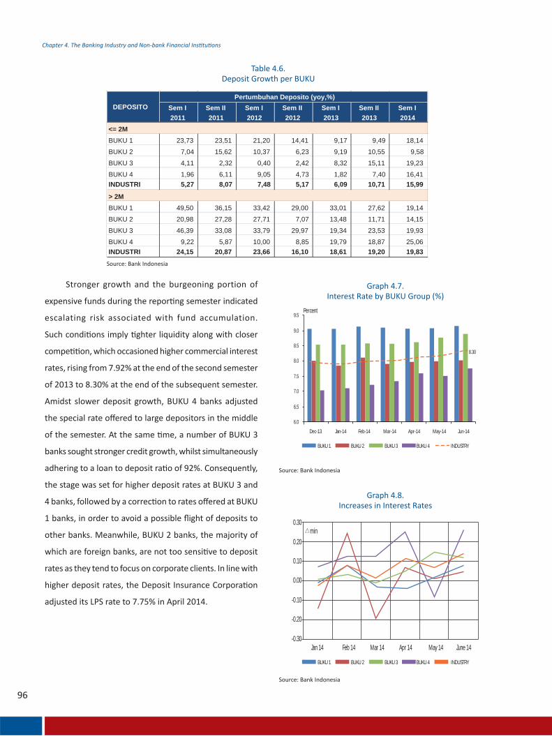
Sem I 2011
Sem II 2011
Sem I 2012
Sem II 2012
Sem I 2013
Sem II 2013
Sem I 2014
<= 2MBUKU 1 23,73 23,51 21,20 14,41 9,17 9,49 18,14
BUKU 2 7,04 15,62 10,37 6,23 9,19 10,55 9,58
BUKU 3 4,11 2,32 0,40 2,42 8,32 15,11 19,23
BUKU 4 1,96 6,11 9,05 4,73 1,82 7,40 16,41 INDUSTRI 5,27 8,07 7,48 5,17 6,09 10,71 15,99
> 2MBUKU 1 49,50 36,15 33,42 29,00 33,01 27,62 19,14
BUKU 2 20,98 27,28 27,71 7,07 13,48 11,71 14,15
BUKU 3 46,39 33,08 33,79 29,97 19,34 23,53 19,93
BUKU 4 9,22 5,87 10,00 8,85 19,79 18,87 25,06 INDUSTRI 24,15 20,87 23,66 16,10 18,61 19,20 19,83
DEPOSITOPertumbuhan Deposito (yoy,%)
9.5Percent
9.0
8.5
8.0
8.30
7.5
7.0
6.5
6.0
Dec-13
BUKU 1
Jan-14 Feb-14 Mar-14 Apr-14 May-14 Jun-14
BUKU 2 BUKU 3 BUKU 4 INDUSTRY
BUKU 1 BUKU 2 BUKU 3 BUKU 4 INDUSTRY
0.30min
0.20
0.10
0.00
-0.10
-0.20
-0.30Jan 14 Feb 14 Mar 14 Apr 14 May 14 June 14

Credit erformance
14.07%
Jul-13
Aug-1
3Se
p-13
Oct-1
3No
v-13
Dec-1
3Jan
-14Fe
b-14
Mar-14
Apr-1
4May-
14
Jun-14
17.20%
7.50%
10%
15%
20%
25%
6%
7%
8%
Semester II 2013 Semester I 2014
BI Rate Credit Growth (yoy. RHS) Adjusted Credit Growth (yoy. RHS)
40%
35
30
25
20
15
10
5
0
Rupiah
I-2013
15.81
24.80
17.20
Foreign Currency Total
II-2013 I-2014
40%
35
30
25
20
15
10
5
0
Working Capital Credit Investment Credit
I-2013
17.30
22.46
12.72
II-2013 I-2014

98
Region 2011 2012 2013 2014
BUKU 1 27.68 28.01 27.65 24.2 22.74 20.84 5.58BUKU 2 27.42 30.56 25.01 21.37 24.64 19.85 26.64BUKU 3 25.46 24.26 19.12 13.56 16.62 16.70 26.09BUKU 4 21.65 23.59 24.00 24.53 22.80 15.42 41.69Industry 24.44 25.75 23.08 20.64 21.60 17.20 100.00
Sem I-2014Credit Growth (%) Sem II-2011 Sem I-2012 Sem II-2012 Sem I-2013 Sem II-2013 Market Share on Semester I-2014 (%)
18.28
13.93
24.9028.61
17.54
25.44
6.18
14.31
6.97
19.53
17.20
05
10152025303540
I-2013 II-2013 I-2014
%
Trad
e
Othe
rsM
anuf
actu
ring
Agric
ultu
reCo
rpor
ate S
ervic
esSo
cial S
ervic
es
Min
ing
Elect
ricity
Tota
l
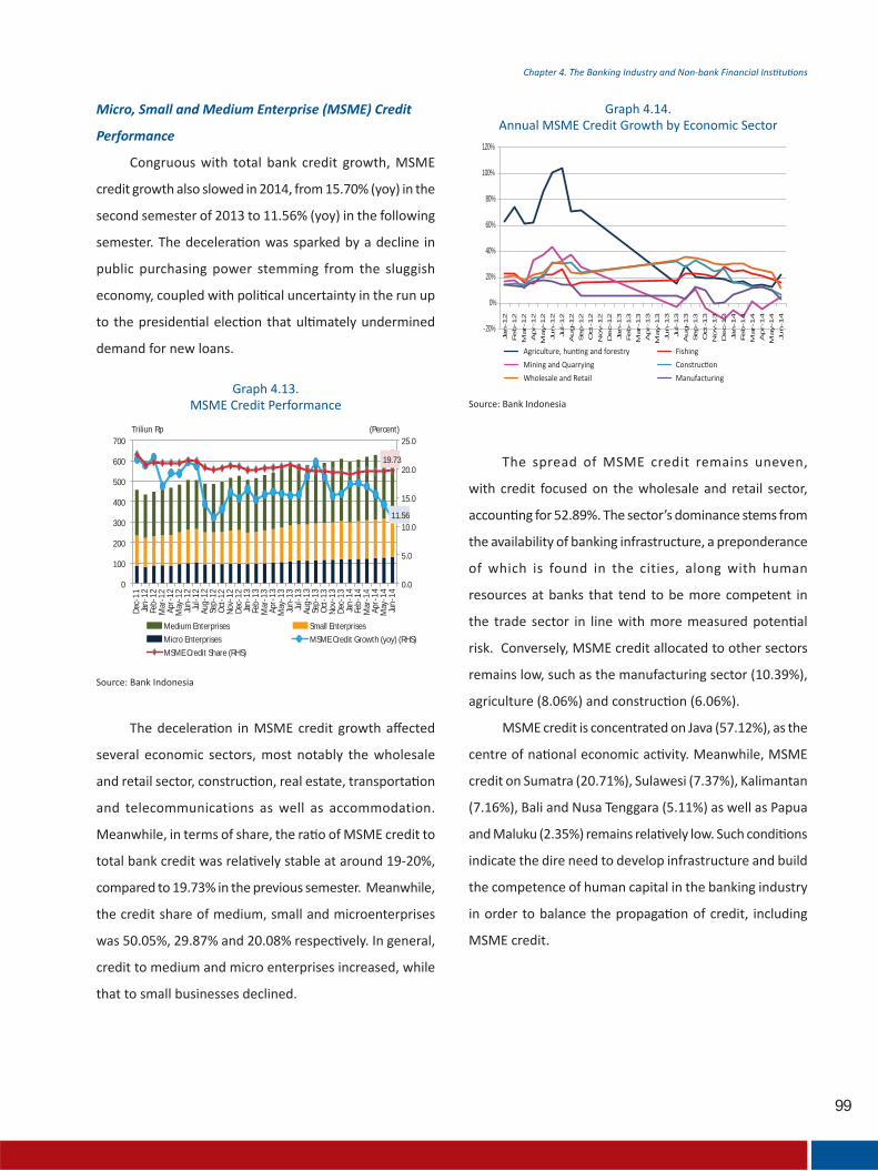
99
icro, mall and edium Enterprise E Credit
erformanceDe
cJa
nFe
bM
ar Apr
May Jun Jul
Aug
Sep
Oct
Nov De
cJa
nFe
bM
ar Apr
May Jun Jul
Aug
Sep
Oct
Nov De
cJa
nFe
bM
ar Apr
May Jun-1
1-1
2-1
2-1
2-1
2-1
2-1
2-1
2-1
2-1
2-1
2-1
2-1
2-1
3-1
3-1
3-1
3-1
3-1
3-1
3-1
3-1
3-1
3-1
3-1
3-1
4-1
4-1
4-1
4-1
4-1
4
11.56
19.73
0.0
5.0
10.0
15.0
20.0
25.0
0
100
200
300
400
500
600
700(Percent)Triliun Rp
Medium Enterprises Small Enterprises
Micro Enterprises MSME Credit Growth (yoy) (RHS)
MSME Credit Share (RHS)
-20%
0%
20%
40%
60%
80%
100%
120%
Jan
-12
Fe
b-1
2
Ma
r-1
2
Ap
r-1
2
Ma
y-1
2
Jun
-12
Jul-
12
Au
g-1
2
Se
p-1
2
Oct-
12
No
v-1
2
De
c-1
2
Jan
-13
Fe
b-1
3
Ma
r-1
3
Ap
r-1
3
Ma
y-1
3
Jun
-13
Jul-
13
Au
g-1
3
Se
p-1
3
Oct-
13
No
v-1
3
De
c-1
3
Jan
-14
Fe
b-1
4
Ma
r-1
4
Ap
r-1
4
Ma
y-1
4
Jun
-14
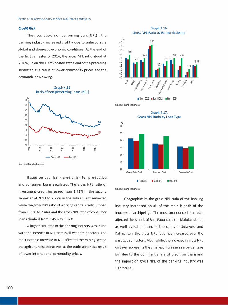
100
Credit isk
2.06
1.11
0.0
0.5
1.0
1.5
2.0
2.5
3.0
3.5
4.0
4.5
2008
2009
2010
2011
2012
2013
2014
%
Gross NPL Net NPL
Trad
e
Othe
rsM
anuf
actu
ring
Agric
ultu
reCo
rpor
ate S
ervic
esSo
cial S
ervic
es
Min
ing
Elect
ricity
Tota
l
2.92
2.002.46
4.24
1.29
2.132.48 2.49
1.06
1.66
0.00.51.01.52.02.53.03.54.04.5
%
Sem I 2013 Sem II 2013 Sem I 2014
0.0
0.5
1.0
1.5
2.0
2.5
3.0%
Sem I 2013 Sem II 2013 Sem I 2014
Working Capital Credit Investment Credit

101
Region Sem I - 2013 Sem II - 2013 Sem I - 2014
Jawa 2.05 1.60 1.67
Sumatera 2.58 2.43 2.87
Kalimantan 2.13 2.47 3.19
Sulawesi 2.60 2.62 3.27
Bali and
and the Islands
Nusa Tenggara 0.93 0.86 1.65
Papua Maluku 2.16 2.07 2.83
Gross NPL (%) Sem II-2011 Sem I-2012 Sem II-2012 Sem I-2013 Sem II-2013 Sem I-2014BUKU 1 2,36 2,38 2,26 2,15 2,41 2,68BUKU 2 2,11 2,14 1,92 2,02 2,02 2,22BUKU 3 2,32 2,3 1,99 2,11 1,94 2,50BUKU 4 2,08 2,09 1,89 1,62 1,43 1,63INDUSTRI 2,17 2,18 1,94 1,88 1,77 2,06
E Credit isk
7.5
13.86
6.7
3.88
-
2.00
4.00
6.00
8.00
10.00
12.00
14.00
16.00
18.00
Jan
-11
Feb
-11
Mar
-11
Apr
-11
May
-11
Jun
-11
Jul-
11A
ug-1
1Se
p-1
1O
ct-1
1N
ov-1
1D
ec-1
1Ja
n-1
2Fe
b-1
2M
ar-1
2A
pr-1
2M
ay-1
2Ju
n-1
2Ju
l-12
Aug
-12
Sep
-12
Oct
-12
Nov
-12
Dec
-12
Jan
-13
Feb
-13
Mar
-13
Apr
-13
May
-13
Jun
-13
Jul-
13A
us-1
3Se
p-1
3O
ct-1
3N
ov-1
3D
ec-1
3Ja
n-1
4Fe
b-1
4M
ar-1
4A
pr-1
4M
ay-1
4Ju
n-1
4
BI Rate MSME NPLLending Rate of MSME Credit
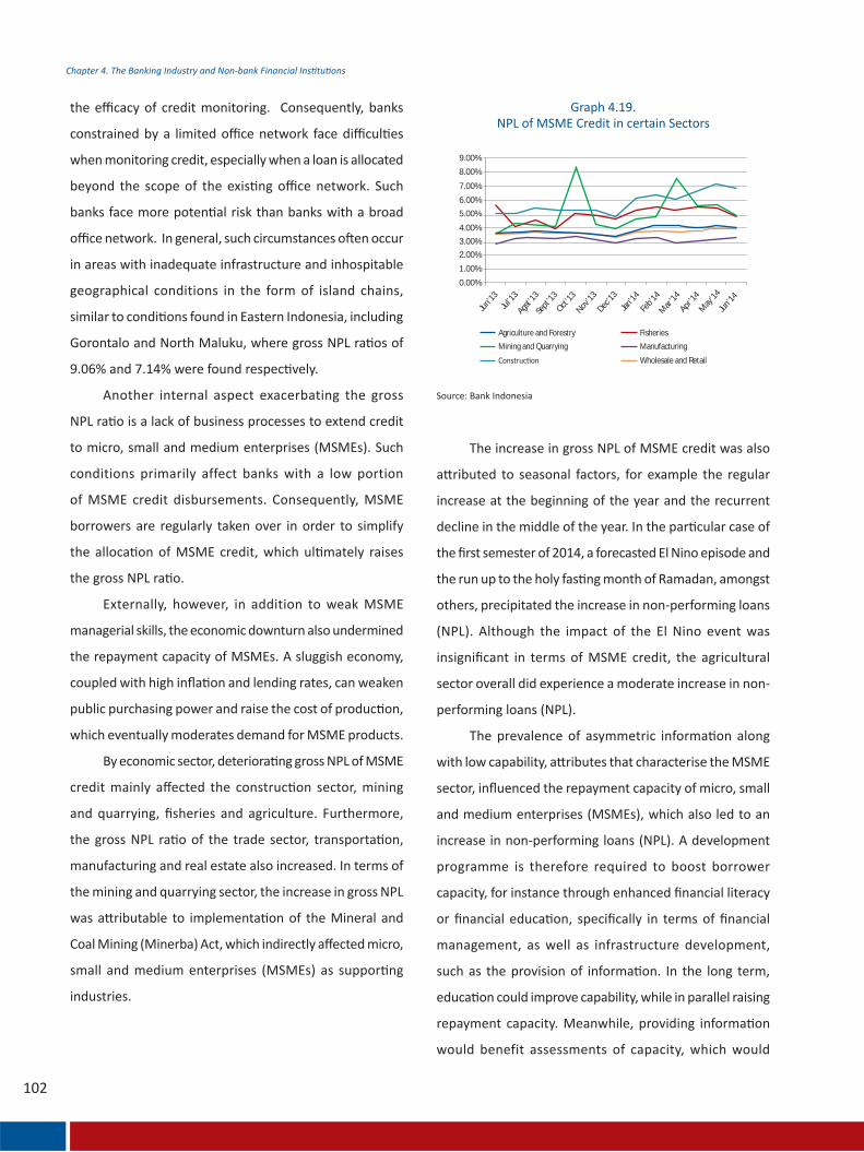
9.00%
8.00%
7.00%
6.00%
5.00%
4.00%
3.00%
2.00%
1.00%
0.00%
Jun’13
Jul’1
3
Sept’1
3Oct
’13Nov’1
3Dec
’13Ja
n’14Fe
b’14M
ar’14
Apr’14
May
’14Ju
n’14
Agst’1
3
Agriculture and Forestry
Mining and Quarrying
Fisheries
Manufacturing
Wholesale and Retail

4.1.3 Market Risk Assessment
Interest ate isk in the Banking Industry
Smt I 2012 Smt II 2012 Smt I 2013 Smt II 2013 Smt I 2014
BUKU 1 6.47 6.79 6.61 9.06 9.14BUKU 2 5.49 5.65 5.69 7.99 8.02BUKU 3 5.59 5.85 5.90 8.54 8.87BUKU 4 4.92 5.05 5.08 7.02 7.76INDUSTRY 5.39 5.58 5.60 7.92 8.30
Smt I 2012 Smt II 2012 Smt I 2013 Smt II 2013 Smt I 2014
BUKU 1 3.24 3.18 3.04 2.70 3.03BUKU 2 2.38 2.17 2.25 2.26 2.54BUKU 3 2.47 2.38 2.37 2.51 2.57BUKU 4 1.89 1.87 1.85 1.80 1.92INDUSTRY 2.27 2.12 2.17 2.12 2.32
Smt I 2012 Smt II 2012 Smt I 2013 Smt II 2013 Smt I 2014
BUKU 1 2.90 2.88 2.76 2.90 2.75BUKU 2 2.91 2.75 3.85 3.94 2.96BUKU 3 2.69 2.61 2.58 2.46 2.58BUKU 4 1.59 1.48 1.42 1.43 1.42INDUSTRY 2.02 1.91 1.99 2.01 1.88
1-month Rupiah Term Deposit Rate
Term Deposit Rate
Savings Deposit Rate
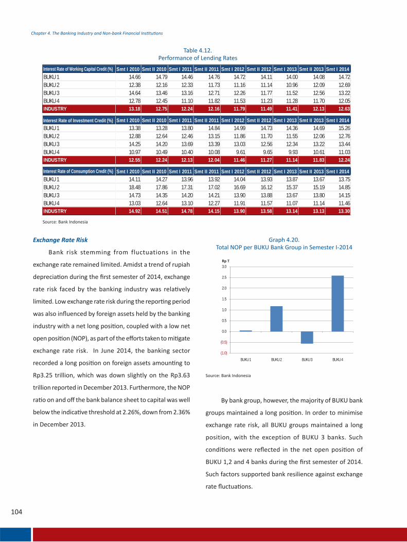
E change ate isk
Smt I 2010 Smt II 2010 Smt I 2011 Smt II 2011 Smt I 2012 Smt II 2012 Smt I 2013 Smt II 2013 Smt I 2014BUKU 1 14.66 14.79 14.46 14.76 14.72 14.11 14.00 14.08 14.72BUKU 2 12.38 12.16 12.33 11.73 11.16 11.14 10.96 12.09 12.69BUKU 3 14.64 13.46 13.16 12.71 12.26 11.77 11.52 12.56 13.22BUKU 4 12.78 12.45 11.10 11.82 11.53 11.23 11.28 11.70 12.05INDUSTRY 13.18 12.75 12.24 12.16 11.79 11.49 11.41 12.13 12.63
Smt I 2010 Smt II 2010 Smt I 2011 Smt II 2011 Smt I 2012 Smt II 2012 Smt I 2013 Smt II 2013 Smt I 2014BUKU 1 13.38 13.28 13.80 14.84 14.99 14.73 14.36 14.69 15.26BUKU 2 12.88 12.64 12.46 13.15 11.86 11.70 11.55 12.06 12.76BUKU 3 14.25 14.20 13.69 13.39 13.03 12.56 12.34 13.22 13.44BUKU 4 10.97 10.49 10.40 10.08 9.61 9.65 9.93 10.61 11.03INDUSTRY 12.55 12.24 12.13 12.04 11.46 11.27 11.14 11.83 12.24
Smt I 2010 Smt II 2010 Smt I 2011 Smt II 2011 Smt I 2012 Smt II 2012 Smt I 2013 Smt II 2013 Smt I 2014BUKU 1 14.11 14.27 13.96 13.92 14.04 13.93 13.87 13.67 13.75BUKU 2 18.48 17.86 17.31 17.02 16.69 16.12 15.37 15.19 14.85BUKU 3 14.73 14.35 14.20 14.21 13.90 13.88 13.67 13.80 14.15BUKU 4 13.03 12.64 13.10 12.27 11.91 11.57 11.07 11.14 11.46INDUSTRY 14.92 14.51 14.78 14.15 13.90 13.58 13.14 13.13 13.30
Interest Rate of Working Capital Credit (%)
Interest Rate of Investment Credit (%)
Interest Rate of Consumption Credit (%)
(1.0)
(0.5)
0.0
0.5
1.0
1.5
2.0
2.5
3.0
BUKU 1 BUKU 2 BUKU 3 BUKU 4
Rp T

isk of ower Tradeable Government ecuri es BN
rices
Period < 12 bulan > 12 bulanJun-12 -1.13 19.29Dec-12 -0.56 19.17Jun-13 0.97 80.09Dec-13 2.77 86.54Jun-14 4.92 83.72
(in trillions of rupiah)
0%
1%
2%
3%
4%
5%
6%
7%
Jun-10 Dec-10 Jun-11 Dec-11 Jun-12 Dec-12 Jun-13 Dec-13 Jun-14
BUKU 1 BUKU 2 BUKU 3 BUKU 4 Industry

4.1.4 Assessment of Pro tability E ciency and Capital
ro tability
BUKU 4 170.82 169.77 148.86 180.23 Trading 1.93 1.88 0.80 1.97 Trading 1.13 1.10 0.54 1.09 AFS 114.12 114.48 108.10 123.26 AFS 66.80 67.43 72.62 68.39 HTM 54.77 53.41 39.95 55.00 HTM 32.06 31.46 26.84 30.51
BUKU 3 32.03 30.97 46.05 51.18 Trading 3.86 4.91 4.46 11.63 Trading 12.05 15.87 9.69 22.73 AFS 23.02 21.00 35.02 30.80 AFS 71.86 67.80 76.05 60.18 HTM 5.15 5.06 6.56 8.75 HTM 16.09 16.33 14.25 17.09
BUKU 2 39.74 60.57 61.12 70.96 Trading 15.09 19.38 10.37 15.05 Trading 37.97 32.00 16.97 21.21 AFS 17.73 26.48 30.85 37.83 AFS 44.61 43.72 50.47 53.31 HTM 6.92 14.71 19.90 18.08 HTM 17.42 24.28 32.56 25.48
BUKU 1 4.22 4.88 5.24 5.81 Trading 0.56 0.34 0.24 0.27 Trading 13.23 7.03 4.55 4.62 AFS 2.16 2.65 2.27 2.09 AFS 51.22 54.31 43.20 35.94 HTM 1.50 1.89 2.74 3.46 HTM 35.55 38.66 52.25 59.45
Industri 246.82 266.20 261.27 308.19 Trading 21.44 26.52 15.88 28.93 Trading 8.69 9.96 6.08 9.39 AFS 157.03 164.61 176.23 193.98 AFS 63.62 61.84 67.45 62.94 HTM 68.35 75.07 69.16 85.28 HTM 27.69 28.20 26.47 27.67
BUKU 1
BUKU 2
BUKU 3
BUKU 4
INDUSTRI
Share of Total (%)
Dec-12 Jun-13 Dec-13 Jun-14
Trading 1.13 1.10 0.54 1.09 AFS 66.80 67.43 72.62 68.39 HTM 32.06 31.46 26.84 30.51
Trading 12.05 15.87 9.69 22.73 AFS 71.86 67.80 76.05 60.18 HTM 16.09 16.33 14.25 17.09
Trading 37.97 32.00 16.97 21.21 AFS 44.61 43.72 50.47 53.31 HTM 17.42 24.28 32.56 25.48
Trading 13.23 7.03 4.55 4.62 AFS 51.22 54.31 43.20 35.94 HTM 35.55 38.66 52.25 59.45
Trading 8.69 9.96 6.08 9.39 AFS 63.62 61.84 67.45 62.94 HTM 27.69 28.20 26.47 27.67
Nominal (Rp T)
Dec-12 Jun-13 Dec-13 Jun-14
BUKU 4 170.82 169.77 148.86 180.23 Trading 1.93 1.88 0.80 1.97 AFS 114.12 114.48 108.10 123.26 HTM 54.77 53.41 39.95 55.00
BUKU 3 32.03 30.97 46.05 51.18 Trading 3.86 4.91 4.46 11.63 AFS 23.02 21.00 35.02 30.80 HTM 5.15 5.06 6.56 8.75
BUKU 2 39.74 60.57 61.12 70.96 Trading 15.09 19.38 10.37 15.05 AFS 17.73 26.48 30.85 37.83 HTM 6.92 14.71 19.90 18.08
BUKU 1 4.22 4.88 5.24 5.81 Trading 0.56 0.34 0.24 0.27 AFS 2.16 2.65 2.27 2.09 HTM 1.50 1.89 2.74 3.46
Industri 246.82 266.20 261.27 308.19 Trading 21.44 26.52 15.88 28.93 AFS 157.03 164.61 176.23 193.98 HTM 68.35 75.07 69.16 85.28
Sem I-2013 Sem II-2013 Sem I-2014 Sem I-2013 Sem II-2013 Sem I-2014 Sem I-2013 Sem II-2013 Sem I-2014 Sem I-2013 Sem II-2013 Sem I-2014
BUKU 1 2.50 1.00 2.5 0.10 0.30 0.01 2.60 1.30 2.49 2.10 0.60 1.97
BUKU 2 13.40 15.90 18.01 1.10 0.70 1.92 14.50 16.50 16.09 11.20 12.10 12.71
BUKU 3 12.10 12.30 13.24 0.30 0.30 0.13 12.40 12.60 13.38 9.50 9.60 10.68
BUKU 4 34.10 40.20 40.46 0.80 2.00 1.06 34.90 42.20 41.52 28.30 33.30 33.07
Industry 62.00 69.50 74.21 2.30 3.30 0.74 64.40 72.70 73.47 51.10 55.60 58.43
Opera onal P/L Non-Opera onal P/L P/l before Tax P/L a er Tax

2014I II I II I II I
88.5 98.9 94.7 107.2 106.5 138.8 134.53.5 4.5 2.9 1.3 2.3 1.2 1.67.5 6.0 6.2 5.5 6.0 8.4 8.7
57.5 73.9 66.8 79.4 77.2 100.1 96.229.4 37.7 33.6 24.8 36.4 30.5 40.1
2.8 4.2 3.2 0.2 1.1 1.0 1.67.1 7.1 8.9 5.5 12.6 20.8 15.58.8 8.0 9.4 10.4 10.6 13.0 13.3
10.8 -1.7 5.3 5.9 5.5 9.4 6.4
Income Account2011 2012 2013
2014I II I II I
91.7 92.0 98.7 116.4 136.11.1 1.5 1.7 2.1 2.2
50.5 50.1 52.9 63.5 79.62.6 2.5 2.8 3.1 3.51.2 1.2 1.2 1.3 1.8
35.9 36.4 39.9 46.0 48.7109.1 109.3 124.9 126.2 138.9
4.5 1.2 2.0 1.0 1.715.2 10.8 21.7 27.0 27.2
3.6 4.0 4.3 4.5 4.824.0 20.3 27.0 14.7 27.429.6 33.4 35.0 36.8 39.616.2 20.0 17.1 20.3 19.4
4.2 13.0 4.4 16.1 6.8
Cost Account2012 2013
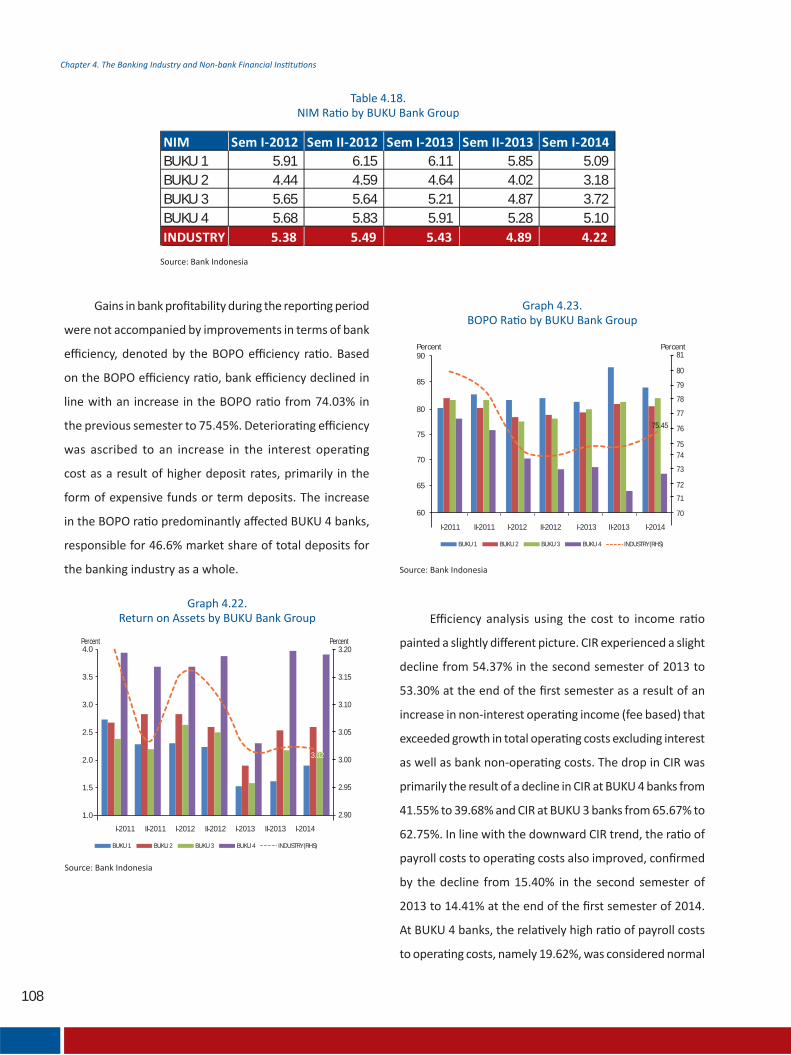
108
NIM Sem I-2012 Sem II-2012 Sem I-2013 Sem II-2013 Sem I-2014BUKU 1 5.91 6.15 6.11 5.85 5.09 BUKU 2 4.44 4.59 4.64 4.02 3.18 BUKU 3 5.65 5.64 5.21 4.87 3.72 BUKU 4 5.68 5.83 5.91 5.28 5.10 INDUSTRY 5.38 5.49 5.43 4.89 4.22
2.90
2.95
3.003.02
3.05
3.10
3.15
3.20
1.0
1.5
2.0
2.5
3.0
3.5
4.0
I-2011 II-2011 I-2012 II-2012 I-2013 II-2013 I-2014
BUKU 1 BUKU 2 BUKU 3 BUKU 4 INDUSTRY (RHS)
Percent Percent
I-2011 II-2011 I-2012 II-2012 I-2013 II-2013 I-2014
BUKU 1 BUKU 2 BUKU 3 BUKU 4 INDUSTRY (RHS)
Percent Percent81
80
79
78
77
75.45 76
7574
73
72
71
70
90
85
80
75
70
65
60

109
Capital
I-2011 II-2011 I-2012 II-2012 I-2013 II-2013 I-2014
BUKU 1 BUKU 2 BUKU 3 BUKU 4 INDUSTRY (RHS)
58.30
65
70Percent
60
55
50
45
40
35
I-2011
Percent
II-2011 I-2012 II-2012 I-2013 II-2013 I-2014
14.41
22
20
18
16
14
12
10
BUKU 1 BUKU 2 BUKU 3 BUKU 4 INDUSTRY

110
4.1.5 Stress Tes ng the Banking Industry
Capital esilience to Credit isk
19.48
15
16
17
18
19
20
0
500
1,000
1,500
2,000
2,500
3,000
3,500
4,000
I-2011 II -2011 I-2012 II -2012 I-2013 II -2013 I-2014
PercentRp T
Capital Risk-Weighted Assets CAR (RHS)
19.48
17.89
12
14
16
18
20
22
24
20
07
20
08
20
09
20
10
20
11
20
12
20
13
20
14
Percent
CAR Tier 1
Industry
Lowest CARHighest CAR Average CAR CAR

111
Capital esilience to arket isk
19.40% 19.33%
26.04%
16.54% 17.10%17.19% 14.11%
20.67%
10.63%
13.98
0%
5%
10%
15%
20%
25%
30%
Industry BUKU 1 BUKU 2 BUKU 3 BUKU 4
Initial CAR NPL of 5% (NPL at individual banks increases 2.32x)NPL of 10% (NPL at individual banks increases 4.63x)NPL of 15% (NPL at individual banks increases 6.95x)
NPL of 7.5% (NPL at individual banks increases 3.48x)NPL of 12.5% (NPL at individual banks increases 5.79x)
-40
-121
- 109
-- 122
-30
-222
-522
- 537
- 591
-312
-700 -600 -500 -400 -300 -200 -100 0
Industry
BUKU 1
BUKU 2
BUKU 3
BUKU 4
NPL of 15% (NPL at individual banks increases 6.95x) NPL of 12.5% (NPL at individual banks increases 5.79x)NPL of 10% (NPL at individual banks increases 4.63x) NPL of 7.5% (NPL at individual banks increases 3.48x)NPL of 5% (NPL at individual banks increases 2.32x)
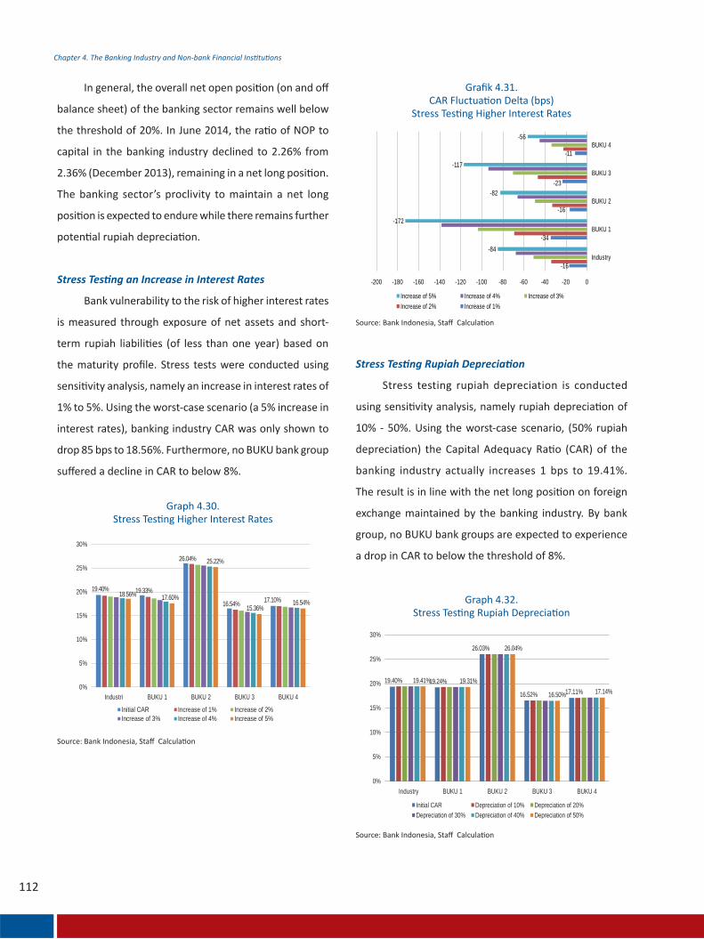
tress Tes ng an Increase in Interest ates
tress Tes ng upiah eprecia on
19.40% 19.33%
26.04%
16.54% 17.10%18.56% 17.60%
25.22%
15.36%16.54%
0%
5%
10%
15%
20%
25%
30%
Industri BUKU 1 BUKU 2 BUKU 3 BUKU 4
Initial CAR Increase of 1% Increase of 2%Increase of 3% Increase of 4% Increase of 5%
-16
-34
-16
-23
-11
-84
-172
-82
-117
-56
-200 -180 -160 -140 -120 -100 -80 -60 -40 -20 0
Industry
BUKU 1
BUKU 2
BUKU 3
BUKU 4
Increase of 5% Increase of 4% Increase of 3%Increase of 2% Increase of 1%
19.40% 19.24%
26.03%
16.52% 17.11%
19.41% 19.31%
26.04%
16.50% 17.14%
0%
5%
10%
15%
20%
25%
30%
Industry BUKU 1 BUKU 2 BUKU 3 BUKU 4
Initial CAR Depreciation of 10% Depreciation of 20%Depreciation of 30% Depreciation of 40% Depreciation of 50%
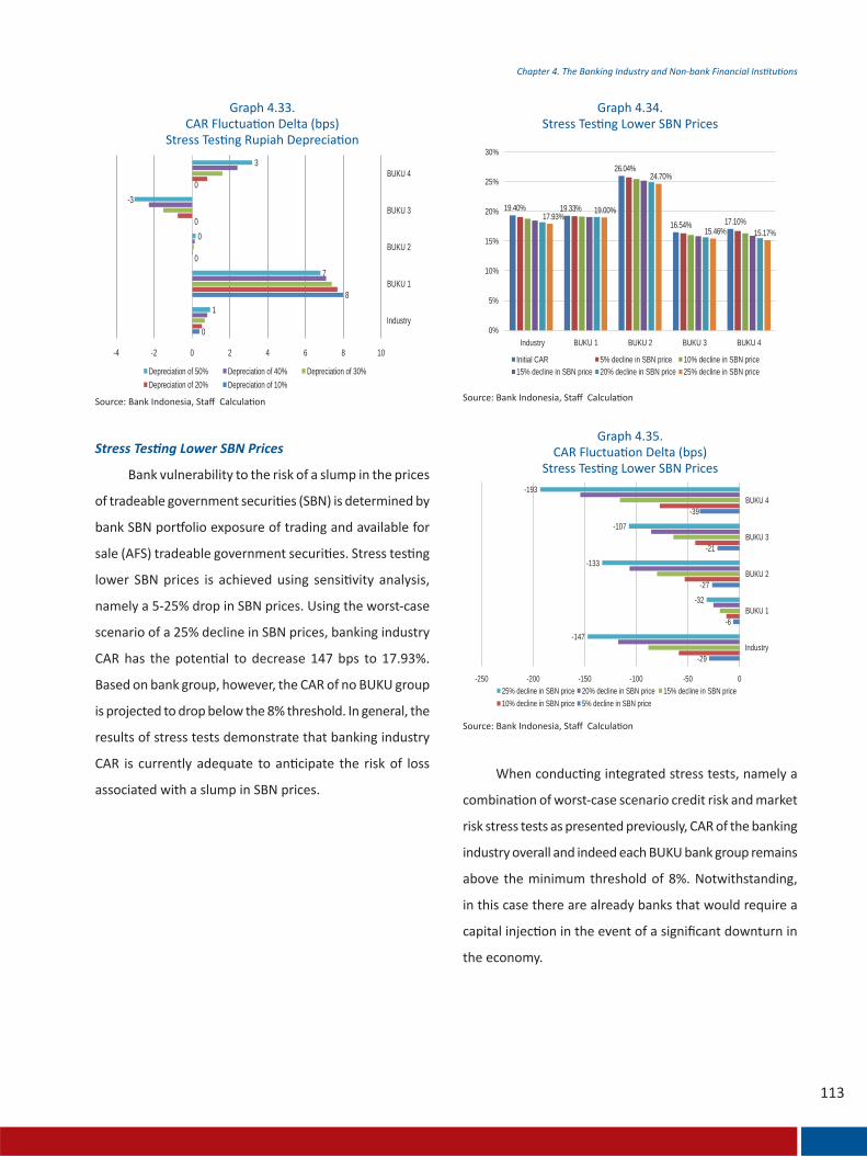
tress Tes ng ower BN rices
0
8
0
0
0
1
7
0
-3
3
-4 -2 0 2 4 6 8 10
Industry
BUKU 1
BUKU 2
BUKU 3
BUKU 4
Depreciation of 50% Depreciation of 40% Depreciation of 30%Depreciation of 20% Depreciation of 10%
19.40% 19.33%
26.04%
16.54% 17.10%17.93%19.00%
24.70%
15.46% 15.17%
0%
5%
10%
15%
20%
25%
30%
Industry BUKU 1 BUKU 2 BUKU 3 BUKU 4
Initial CAR 5% decline in SBN price 10% decline in SBN price15% decline in SBN price 20% decline in SBN price 25% decline in SBN price
-29
-6
-27
-21
-39
-147
-32
-133
-107
-193
-250 -200 -150 -100 -50 0
Industry
BUKU 1
BUKU 2
BUKU 3
BUKU 4
25% decline in SBN price 20% decline in SBN price 15% decline in SBN price10% decline in SBN price 5% decline in SBN price

4.2 NON BANK FINANCIAL INSTITUTIONS NBFI
4.2.1 Finance Companies (FC)
(Rp. T)
250 28
23
18
13
8
3
(2)
200
150
10077
165
102
179
105 106
192
210
117
223
116
237
50
Dec’11
Leasing
Jun’12 Dec’12 Jun’13 Dec’13 Jun’14
-
(Rp. T)
Consumer Financing Factoring
4 45 5
8 8
(Rp. T)
450
350
400
250
300
200
150
100
245
291
50
Dec’11
Assets
Jun’12 Dec’12 Jun’13 Dec’13 Jun’14-
Financing
284
322302
342321
359348
401
361
4133,00%
2,50%
2,00%
1,50%
1,99%
2,29%
2,00%
2,16%
2,03%
2,48%
2,29%
1,85%1,62%
1,33%1,47%
1,00%
0,50%
0,00%
Des’11
Mar
’12
Jun’
12
Sep’
12
Des’12
Mar
’13
Jun’
13
Sep’
13
Des’13
Mar
’14
Jun’
14
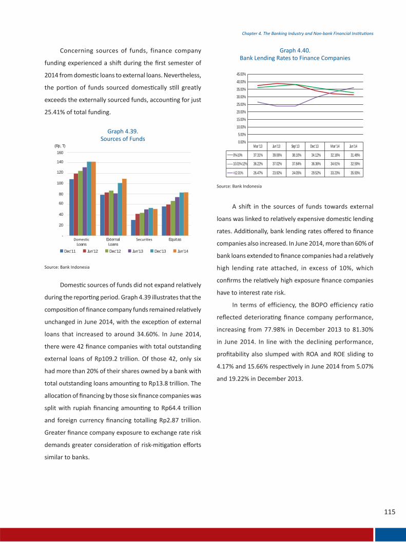
(Rp, T)
Dec'11 Jun'12
Loans
160
140
120
100
80
60
40
20
-External
LoansEquitas
Dec'12 Jun'13 Dec'13 Jun'14
45.00%
40.00%
35.00%
30.00%
25.00%
20.00%
15.00%
10.00%
5.00%
0.00%Mar’13
37.31%
36.22%
26.47%
39.06%
37.02%
23.92%
38.10%
37.84%
24.05%
34.12%
36.36%
29.52%
32.16%
34.61%
33.23%
31.48%
32.59%
35.93%
Jun’13 Sep’13 Dec’13 Mar’14 Jun’14
0%-10%
10.01%-12%
>12.01%

4.2.2 Insurers1
Licensed
PT Asuransi Jiwa Indosurya Sukses 11 September 2013
PT Asuransi Agrapana Aksata Januari 2013
PT Central Asia Financial March 2013
Company Name
25.00% 82.00%
81.00%
80.00%
79.00%
78.00%
77.00%
76.00%
75.00%
20.00%
15.00%
10.00%
5.00%
0.00%
ROA
Mar’13
4.96%
20.00%
78.34%
Jun’13
5.08%
19.83%
77.74%
Sep’13
5.16%
19.79%
77.40%
Des’13
5.07%
19.22%
77.98%
Mar’14
4.47%
16.78%
79.56%
Jun’14
4.17%
15.66%
81.30%
ROE
BOPO
25%
16%15%
44%
Life insurance General Insurance and Reinsurance
ocial Insurance Programmesand Social Insurance forPrivate Sector Workers
Insurers of Civil Servants,Army Personnel and the Police
481.75
569.32
652.9
419.7
497.03521.97
87.12% 87.30%
79.95%
50%
55%
60%
65%
70%
75%
80%
85%
90%
0
100
200
300
400
500
600
700
2011 2012 2013
Rp Trillion
Assets Investments
87.79
109.62121.67
153.13
178.07
198.53
57.33%
61.56% 61.29%
25%
30%
35%
40%
45%
50%
55%
60%
65%
0
20
40
60
80
100
120
140
160
180
200
2011 2012 2013*
Rp Trillion
Gross Claims Gross Premiums

Life Insurance
Total
State-Owned
PrivateNa onal
JointVenture
Insurance Pro le Total
Loss Insurance
Reinsurance
11 93 37 141
Social Insurance Programmes and Social Insurance for Private Sector Workers
Insurers of Civil Servants, Army Personnel and the Police
1 29 19 493 62 18 832 2 4
2
3
2
3
Thousand Rp800
2008 2009 2010 2011 2012 2013*
%25
25
15
10
5
0
700
600
500
400
300
200
100
0
Density Growth
19.6817.51
22.37
13.74
0.27
11.41
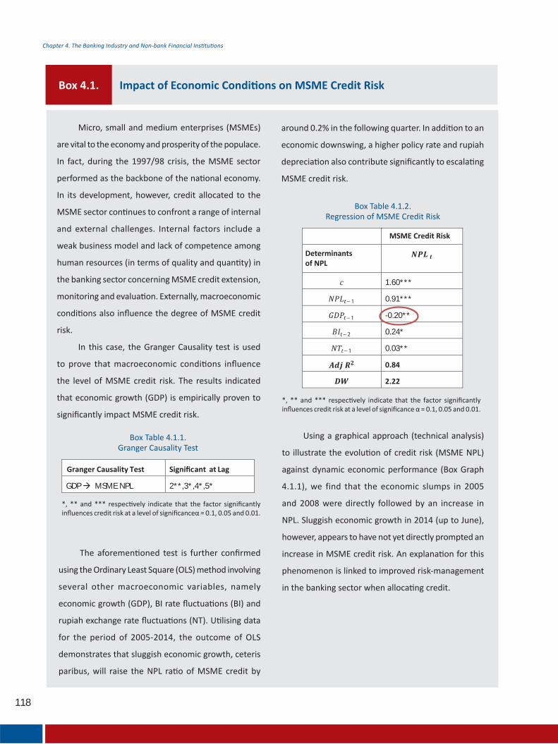
118
Box 4.1. Impact of Economic Condi ons on MSME Credit Risk
Test Granger Causality Signi cant at Lag
GDP NMSME PL 2**,3*,4*,5*
1.60***
− 1 0.91***
− 1 -0.20**
− 2 0.24*
− 1 0.03**
0.84
2.22
Determinantsof NPL
MSME Credit Risk

119
10.0
9.0
8.0
7.0
6.0
5.0
4.0
3.0
2.0
MSME NPL (%) on-MSME NPL (%) GDP (% yoy)
1.0
Mar
-03
Sept
-03
Mar
-04
Sept
-04
Mar
-05
Sept
-05
Mar
-06
Sep-
06M
ar-0
7Se
pt-0
7
Mar
-08
Sept
-08
Mar
-09
Sept
-09
Mar
-10
Sept
-10
Mar
-11
Sept
-11
Mar
-12
Sept
-12
Mar
-13
Sept
-13
Mar
-14

Box 4.2 The Role of Educa on and Provision of Informa on to derail the Upward NPL Trend
Financial Iden ty Number
Financial Educa on
Informa on System for Farmers and Fishermen
(SIPN)

123
Chapter 5. Financial System Infrastructure
Financial System Infrastructure
Chapter 5

124
Chapter 5. Financial System Infrastructure

125
Chapter 5. Financial System Infrastructure
5.1 PAYMENT SYSTEM PERFORMANCE
5.1.1 The Payment System Operated by Bank Indonesia
Financial System InfrastructureChapter5

Chapter 5. Financial System Infrastructure
5.1.2 The Industry-Operated Payment System
5.2 PAYMENT SYSTEM TRANSACTION PERFORMANCE
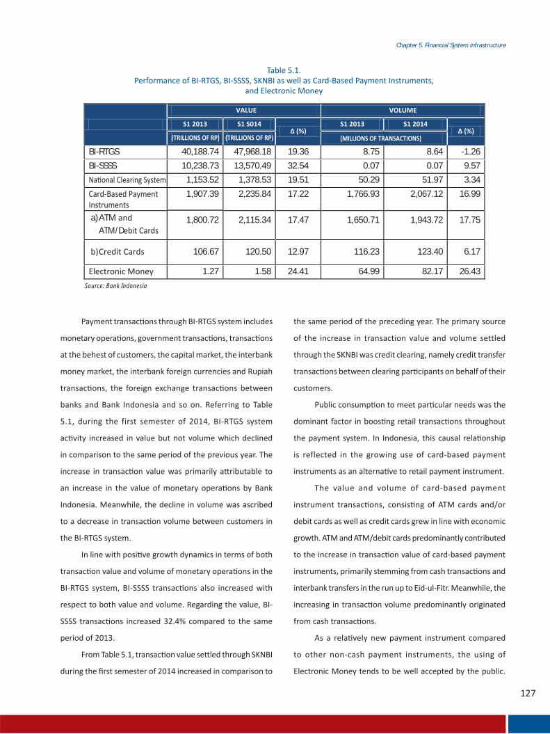
Chapter 5. Financial System Infrastructure
VALUE VOLUME
S1 2013 S1 S014 (%)
S1 2013 S1 2014 (%)
BI-RTGS 40,188.74 47,968.18 19.36 8.75 8.64 -1.26
BI-SSSS 10,238.73 13,570.49 32.54 0.07 0.07 9.57
1,153.52 1,378.53 19.51 50.29 51.97 3.34
1,907.39 2,235.84 17.22 1,766.93 2,067.12 16.99
a)ATM ATM/D
1,800.72 2,115.34 17.47 1,650.71 1,943.72 17.75
106.67 120.50 12.97 116.23 123.40 6.17
1.27 1.58 24.41 64.99 82.17 26.43
Source: Bank Indonesia
(TRILLIONS OF RP) (TRILLIONS OF RP) (MILLIONS OF TRANSACTIONS)
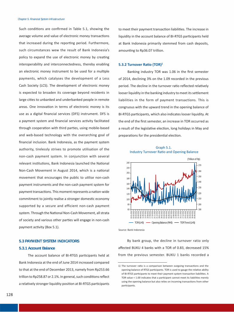
Chapter 5. Financial System Infrastructure
5.3 PAYMENT SYSTEM INDICATORS
5.3.1 Account Balance
1
(Trillion of Rp)
TOR (LHS)
240270
260
250
240
230
220
210
200
190
220
200
180
160
140
120
100
80
60
02-0
1-20
1202
-02-
2012
05-0
3-20
1205
-04-
2012
08-0
5-20
1211
-06-
2012
11-0
7-20
1210
-08-
2012
17-0
9-20
1217
-10-
2012
21-1
1-20
1221
-12-
2012
29-0
1-20
1228
-02-
2012
03-0
4-20
1203
-05-
2012
05-0
6-20
1208
-07-
2012
12-0
8-20
1211
-09-
2012
11-1
0-20
1215
-11-
2012
17-1
2-20
1222
-01-
2012
24-0
2-20
1226
-03-
2012
30-0
4-20
1205
-06-
2012
TOR Trend (LHS)Opening Balance (RHS)

Chapter 5. Financial System Infrastructure
0,00
0,50
1,00
1,50
2,00
2,50
BUKU 1 BUKU 2 BUKU 3 BUKU 4 Industri
2012 Sem I 2012 Sem II 2013 Sem I 2013 Sem II 2014 Sem I
2 2012 Sem I 2012 Sem II 2013 Sem I 2013 Sem II 2014 Sem I
0.00
0.50
1.00
1.50
2.00
2.50
BUKU 1 BUKU 2 BUKU 3 BUKU 4 Industry
Millions of Rp
2012 Sem I 2012 Sem II 2013 Sem I 2013 Sem II 2014 Sem I
0
4000
3000
2000
1000
BUKU 1 BUKU 2 BUKU 3 BUKU 4 Industry
Chapter 5. Financial System Infrastructure
5 5.4 PAYMENT SYSTEM RISK AND MITIGATION EFFORTS
3
5.4.2 Liquidity Risk4

131
Chapter 5. Financial System Infrastructure
Box 5.1
132
Chapter 5. Financial System Infrastructure

133
Ar cle1. Banking Model of Bank Indonesia - BAMBI
2. LDR-linked RR Policy to Support Countercyclicality in the Op misa on of Intermedia on and Minimisa on of Liquidity Risk

134

135
1. INTRODUCTION
4
2. MODEL STRUCTURE AND ESTIMATION RESULTS
2.1 Model Structure
Banking Model of Bank Indonesia - BAMBI1
Ar cle 1
Ndari Sur aningsih2 dan Tevy Chawwa3

a. Interac on between the Macroeconomic and
Banking Sector
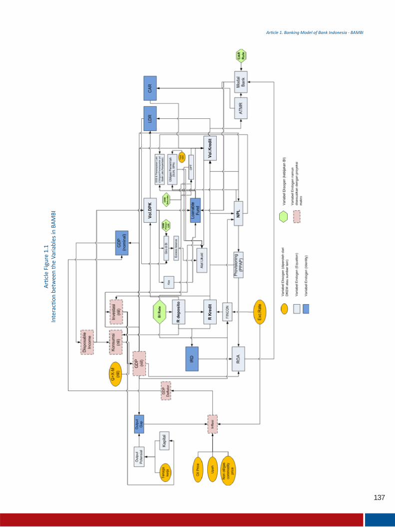
137

138
b. Interac on between Variables in the Banking Sector
2.2 METHODOLOGY
2.3 Es ma on Results
5 The
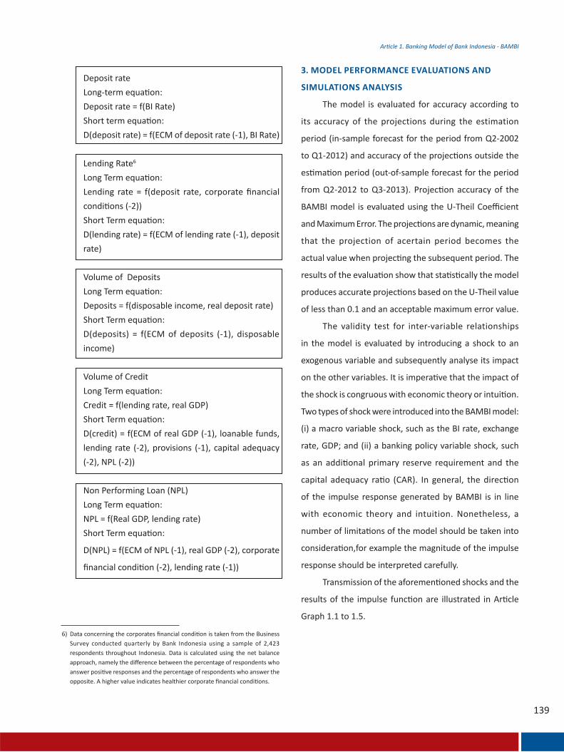
3. MODEL PERFORMANCE EVALUATIONS AND
SIMULATIONS ANALYSIS


141

4. MODEL LIMITATIONS
7

143
5. CONCLUSION REFERENCES

145
Article 2. KLDR-linked RR Policy to Support Countercyclicality in the Optimisationof Intermediation and Minimisation of Liquidity Risk
1. INTRODUCTION
In Indonesia, bank credit remains a key factor in terms
of funding corporate investment and working capital. The
banking system dominates 75-80% of assets in the financial
system, which leads authorities to ensure that bank credit
extension is constantly optimal in support of the economy.
From a macroprudential standpoint, the ratio of credit to
deposits, or the Loan-to-Deposit ratio (LDR), illustrates
liquidity conditions in the banking sector. In general, deposits
are short term and must be available for withdrawal at any
time by depositors. In contrast, credit is relatively long term,
nearly always longer term than deposits, requiring time to be
repaid. As more credit is disbursed in comparison to deposits,
liquidity risk can manifest when depositors withdraw their
funds.
2. ECONOMIC RATIONALE OF MACROPRUDENTIAL
POLICY
2.1. Economic Rationale
Bank management will always strive to maximise profit
in order to maximise shareholder value as the overarching
goal of providing value added to the shareholders and
minimisingthe possibility of losing managerial position
in the operating activity of the bank. On the other hand,
bank supervisors are in a position to assure operational
sustainability of the banks that fall under their supervisory
activities . In general, economic and financial policy
can be divided into four main areas: microprudential,
macroprudential, monetary and macroeconomic policy (refer
to Table 1).
In terms of microprudential, supervisors of financial
institutions tend to place safety factors higher in order to
ensure that a bank is adequately resilient in the face of future
financial disruption. That explains why bank management
tends to emphasise safety factors, which can be viewed as
imprudent behaviour or worse bordering on fraud. The main
aim of microprudential policy is to optimise operational
efficiency at a bank and concomitantly ensure that the bank
maintains its risk-taking capacity, supported by sound risk
management and good corporate governance. Typically, all
information concerning the operational soundness of a bank
is contained within the bank soundness rating report.
LDR-linked RR Policy to Support Countercyclicality in the Optimisation of Intermediation and
Minimisation of Liquidity Risk1
Article 2
Dadang Muljawan2, Cicilia Anggadewi Harun3, Aditya Anta Taruna4
1) The opinions expressed in this paper are those of the authors and not those of Bank Indonesia.2) Senior Economic Researcher, Macroprudential Policy Department, Bank Indonesia; Email:
[email protected]) Senior Economic Researcher, Macroprudential Policy Department, Bank Indonesia; Email:
[email protected]) Economic Researcher, Macroprudential Policy Department, Bank Indonesia; Email: aditya_at@
bi.go.id

146
Article 2. KLDR-linked RR Policy to Support Countercyclicality in the Optimisationof Intermediation and Minimisation of Liquidity Risk
Concerning macroprudential pol icy, deeper
consideration is required over the longer term.
Macroprudential policy not only deals with the operational
sustainability of a bank but also systemic stability that
correlates with other variables. Countercyclical policy at
times can be considered not to support bank management
efficiency because banks are required to maintain larger
reserves when economic conditions are actually favourable.
A similar perception is also found in terms of liquidity risk
management, where banks are encouraged to maintain a
larger buffer when profits from loans are higher.
Monetary policy aims to achieve price stability through
monetary operations and implement the function of Lender
of Last Resort (LOLR) in order to ensure an adequate
level of liquidity, thereby enabling effective monetary
operations. Macroeconomic policy, in general, is instituted
by the government to create aconduciveenvironment to the
production of goods and provision of services. Such policy
encompasses policy in the fiscal sector, minimum wages
and various other policies related to real sector activity. The
differences between macroeconomic and macroprudential
policy can be observed from two main perspectives, namely
the countercyclicality impact produced and sector-based
policy. The core of countercyclicality in financial policy is to
compile an appropriate incentive scheme for market players
in order that they might prepare themselves to confront
future uncertainty and to encourage them to contribute
to a national economic recovery. Sector-based policy is
policymaking that refers to the different dynamics in each
sector, which might require differing policy incentives, for
example variable LTV policy (loan-to-value) in each target
sector. In terms of monetary policy, sector-based policy can
be considered less effective as interest rate and exchange rate
policy is aggregate in nature and aims to impact the system
as a whole. Meanwhile, for banking supervisors, the core of
the policy taken is to ensure operational continuity at the
institutional level.
2.2. LDR-linked RR Policy
Originally, the reserve requirement (RR) was a monetary
instrument that aimed to control bank credit. The reserve
requirement functioned to provide bank liquidity in order
to reduce credit allocation. Notwithstanding, as sources of
deposits became more diverse, the reserve requirement
became less effective at reducing the banks’ ability to extend
credit. Despite losing power in terms of reducing credit
allocation, the reserve requirement remained a powerful
instrument for the authorities becauseits capability to impose
Area Target Remarks
Microprudential Risk absorption capacity and efficiency Optimise banking sector operations and risk absorption capacity, supported
by sound risk management practise and good corporate governance. Such
information is usually available from the bank soundness rating system.
Macroprudential Financial system stability Policy that encompasses microprudential and macroprudential policy.
Monetary Price Stability Optimise monetary instruments in order to achieve price stability through
interest rate and exchange rate policy..
Macroeconomic Growth and Unemployment Optimise infrastructure in order to achieve robust economic growth
through fiscal management, including tax policy, sectoral growth,
minimum wages, etc.
Article Table 2.1. Description of Regulatory Regimes

147
Article 2. KLDR-linked RR Policy to Support Countercyclicality in the Optimisationof Intermediation and Minimisation of Liquidity Risk
penalties that directly impact bank liquidity and can also
provide clear signals to the banking industry in support of
economic growth. Consequently, the RR was subsequently
supplemented with additional features aimed at controlling
bank credit growth. In this case, bank behaviour in terms
of extending credit is reflected by the loan-to-deposit ratio
(LDR). The correlation between the RR and LDR is illustrated
in Figure 1.
Lower Limit
In general, LDR is used to illustratesthe level of
efficiency at a bank in terms of the intermediation function.
In a traditional economic system, a low LDR level reflects
a low level of intermediation, implying that the economy
requires a capital injection to bolster activity and economic
growth. Hitherto, however, there is no instrument to maintain
intermediation at a level desired by the authority. During a
contractionary economic phase, the level of return of credit
might be lower than the level of return offered by financial
assets. Therefore, enforcing a high LDR is perceived as
inefficient by the banks and by the supervisory authority too
because the regulation encourages banks to extend more
credit that is, in fact, less profitable. From a macroprudential
standpoint, however, such regulations could save the
economic system from a deeper contraction, into a recession,
and provide an opportunity for economic recovery. The idea
behind applying a higher reserve requirement is to provide a
disincentive to banks with a low loan-to-deposit ratio5.
(E.1)
As shown in Equation 1, banks with a loan-to-deposit
ratio below the threshold, ( ), will be required to place
loanable funds at the central bank in the event they cannot
extend their funds to economic sectors. P0 represents primary
reserves and P1 is the increase in the reserve requirement
due to a bank’s inability to meet the minimum LDR (lower
limit). This can be considered an indirect penalty because
the bank will experience a higher cost of capital whilst their
funds remain idle at the monetary authority.
Upper limit
A high LDR (surpassing the upper limit) indicates
excessive lending, where credit disbursed exceeds the funds
accumulated from the customers. Such conditions imply
that a portion of the bank’s capital is also utilised in the
extension of credit. Excessive lending is undesirable to the
supervisory authority because it can undermine bank liquidity
conditions and bank infrastructure development. During an
5) Historically, the lowest level of LDR in Indonesia was 60% during the recovery period after the 1998 crisis. At that time, banks were unwilling to extend credit due to the perception of high credit risk.
Artikel 2. Kebijakan GWM-LDR Untuk Mendukung Countercyclicality…
𝑅𝑅𝑅𝑅𝑅𝑅𝑅𝑅 = 𝜌𝜌𝜌𝜌0 + 𝜌𝜌𝜌𝜌1 𝑑𝑑𝑑𝑑𝑙𝑙𝑙𝑙 , when 𝑙𝑙𝑙𝑙𝑑𝑑𝑑𝑑 < 𝑙𝑙𝑙𝑙𝑑𝑑𝑑𝑑 (P.1)
Sebagaimana ditunjukkan pada persamaan (P.1), bank yang memiliki LDR dibawah threshold 𝑙𝑙𝑙𝑙𝑑𝑑𝑑𝑑akan
diwajibkan untuk menyimpan loanable fund yang dimiliki di otoritas moneter jika mereka tidak dapat menyalurkan dananya ke dalam sektor ekonomi. 𝜌𝜌𝜌𝜌0merepresentasikanprimary RR dan 𝜌𝜌𝜌𝜌1merepresentasikan kenaikan RR karena bank tidak dapat memenuhi minimum LDR (batas bawah). Ini dapat dianggap sebagai bentuk indirect penaltykarena bank akan mengalami tingkat biaya capital yang lebih tinggi ketika dana mereka ditahan idle di otoritas meneter. Batas atas (Upper limit) Tingginya LDR (diatasbatas atas) menggambarkan excessive lendingdimana kredit yang diberikan melampaui dana yang dikumpulkan dari nasabah. Hal ini berarti sebagian modal yang dimiliki bank juga digunakan untuk mendukung pemberian kredit. Pemberian kredit yang berlebihan juga tidak diinginkan oleh otoritas pengawasan karena hal itu dapat berakibat buruk pada kondisi likuiditas bank dan proses pembangunan infrastruktur bank. Dalam kondisi economic boom, bank mungkin saja memaksimalkan pemberian kreditnya untuk mengoptimalkan keuntungan yang ingin dicapai. Dalam kondisi demikian, bank cenderung untuk meminimalkan likuiditas (termasuk instrumen likuiditas) karena tingkat return yang didapat dari kredit lebih tinggi. Pengawas bank akan menetapkan threshold tertentu sebagai posisi likuiditas minimum untuk memastikan bahwa bank selalu berada dalam kondisi yang sehat dalam memenuhi kewajiban jangka pendeknya. Regulasi seperti ini akan dianggap tidak efisien oleh manajemen bank karena berusaha untuk menekan ekspansi kredit. Hal ini menunjukkan bahwa, pada area tertentu, otoritas pengawasan dan manajemen bank selalu berada pada natural conflict guna mengoptimalkan pencapaian tujuan masing-masing.Otoritasmakroprudensial bahkan dapat berada pada posisi yang lebih berhati-hati lagi mengingat mereka tidak hanya memperhatikan masalah kesinambungan operasi bank sebagai institusi, namun juga kestabilan sistem keuangan yang dapat dirusak oleh gagalnya satu bank. Oleh karena itu, untuk mengisi kekosongan tujuan kebijakan, instrumen kebijakan makroprudensial diterapkan.
Gambar3 a) Probability of liquidity problem6 b) Total return of the bank
6Probability of Liquidity Problem (probabilitas masalah likuiditas) diasumsikan terdistribusi secara Poisson distribusi untuk menggambarkan behavioraldi pasar keuangan dan dampak terhadap bank akibat diskon harga yang berlaku.
144
Gambar1
Kerangka LDR-linked Reserve Requirement
RR
LDR
Primary RR
Optimal LDR
Theoretical FrameworkRR
LDR
Primary RR
Lowerlimit
Upperlimit
Framework Design
Article Graph 2.1. LDR-linked Reserve Requirement Framework
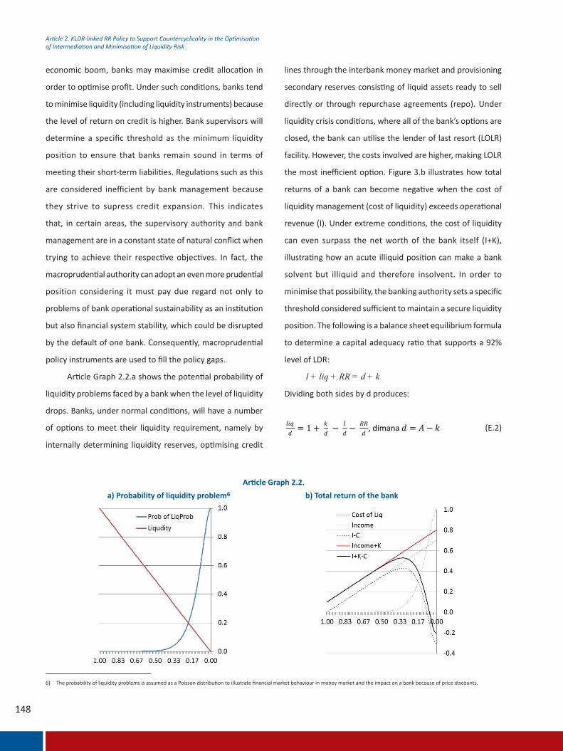
148
Article 2. KLDR-linked RR Policy to Support Countercyclicality in the Optimisationof Intermediation and Minimisation of Liquidity Risk
economic boom, banks may maximise credit allocation in
order to optimise profit. Under such conditions, banks tend
to minimise liquidity (including liquidity instruments) because
the level of return on credit is higher. Bank supervisors will
determine a specific threshold as the minimum liquidity
position to ensure that banks remain sound in terms of
meeting their short-term liabilities. Regulations such as this
are considered inefficient by bank management because
they strive to supress credit expansion. This indicates
that, in certain areas, the supervisory authority and bank
management are in a constant state of natural conflict when
trying to achieve their respective objectives. In fact, the
macroprudential authority can adopt an even more prudential
position considering it must pay due regard not only to
problems of bank operational sustainability as an institution
but also financial system stability, which could be disrupted
by the default of one bank. Consequently, macroprudential
policy instruments are used to fill the policy gaps.
Article Graph 2.2.a shows the potential probability of
liquidity problems faced by a bank when the level of liquidity
drops. Banks, under normal conditions, will have a number
of options to meet their liquidity requirement, namely by
internally determining liquidity reserves, optimising credit
lines through the interbank money market and provisioning
secondary reserves consisting of liquid assets ready to sell
directly or through repurchase agreements (repo). Under
liquidity crisis conditions, where all of the bank’s options are
closed, the bank can utilise the lender of last resort (LOLR)
facility. However, the costs involved are higher, making LOLR
the most inefficient option. Figure 3.b illustrates how total
returns of a bank can become negative when the cost of
liquidity management (cost of liquidity) exceeds operational
revenue (I). Under extreme conditions, the cost of liquidity
can even surpass the net worth of the bank itself (I+K),
illustrating how an acute illiquid position can make a bank
solvent but illiquid and therefore insolvent. In order to
minimise that possibility, the banking authority sets a specific
threshold considered sufficient to maintain a secure liquidity
position. The following is a balance sheet equilibrium formula
to determine a capital adequacy ratio that supports a 92%
level of LDR:
l + liq + RR = d + k
Dividing both sides by d produces:
(E.2)
6) The probability of liquidity problems is assumed as a Poisson distribution to illustrate financial market behaviour in money market and the impact on a bank because of price discounts.
Artikel 2. Kebijakan GWM-LDR Untuk Mendukung Countercyclicality…
Gambar3.amenunjukkan potensi probability of liquidity problem(probabilitas masalah likuiditas) yang akan dihadapi bank ketika tingkat likuiditas menurun. Bank, dalam kondisi normal, akan memiliki beberapa pilihan dalam memenuhi kebutuhan likuiditasnya yaitu dengan menetapkan cadangan likuiditas secara internal, mengoptimalkan credit line melalui pasar uang antar bank, membentuk secondary reserve yang terdiri dari liquid assetsyang siap untuk dijual secara langsung maupun melalui mekanisme repo.Dalam kondisi darurat likuiditas, dimana seluruh pilihan bank telah tertutup, bank bisa memanfaatkan fasilitas LOLR.Namun demikian, biaya yang dibutuhkan akan semakin tinggi sehingga menempatkan fasilitas LOLR sebagai opsi yang paling tidak efisien untuk didapat. Gambar3.bmenunjukkan bagaimana total returnsdari dari bank menjadi negatif ketika biaya yang ditimbulkan dari manajemen likuiditas (cost of liquidity) melebihi operational revenue (I). Dalam kondisi yang ekstrim,cost of liquiditymungkin saja melebihi networth bank (I + K) yang menggambarkan bagaimana posisi illikuid yang akut dapat membuat bank yang solvent namun tidak likuid menjadi tidak solvent. Untuk meminimalkan kemungkinan tersebut, otoritas perbankan menentukan threshold tertentu yang dipercaya dapat menjaga posisi likuiditasnya secara aman. Berikut adalah formulasi kesetimbangan balance sheet untuk mendapatkan angka Capital Adequacy Ratio (CAR)yang dapat menunjang 92% LDR: 𝑙𝑙𝑙𝑙 + 𝑙𝑙𝑙𝑙𝑙𝑙𝑙𝑙𝑙𝑙𝑙𝑙 + 𝑅𝑅𝑅𝑅𝑅𝑅𝑅𝑅 = 𝑑𝑑𝑑𝑑 + 𝑘𝑘𝑘𝑘 Membagi kedua sisi dengan d, kita mendapatkan 𝑙𝑙𝑙𝑙𝑙𝑙𝑙𝑙𝑙𝑙𝑙𝑙𝑑𝑑𝑑𝑑 = 1 + 𝑘𝑘𝑘𝑘𝑑𝑑𝑑𝑑 − 𝑙𝑙𝑙𝑙𝑑𝑑𝑑𝑑 − 𝑅𝑅𝑅𝑅𝑅𝑅𝑅𝑅𝑑𝑑𝑑𝑑 , dimana 𝑑𝑑𝑑𝑑 = 𝐴𝐴𝐴𝐴 − 𝑘𝑘𝑘𝑘 (P.2)
Menentukan posisi likuiditas aman sebesar 8%7dengan RR sebessar 8%, didapatkan nilai berikut:
0.13 = 𝑘𝑘𝑘𝑘𝐴𝐴𝐴𝐴−𝑘𝑘𝑘𝑘 atau 𝑘𝑘𝑘𝑘𝐴𝐴𝐴𝐴 = 0.115
Dengan rasio aktiva tertimbang menurut risikosebesar 80%, nilai optimum CAR yang dapat mendukung 92% percent LDR dengan pemenuhan 8% RR and 8% likuiditas adalah 14.38%.
Gambar4 Probability of liquidity problem8
7Analisa base line menunjukkan bahwa likuiditas optimal berarti bank memiliki kemampuan menyerap shock dengan mempertahan kan efisiensi berada di angka 8% (threshold oleh rasio AL/DPK). 8Simulasi di Gambar 3 dilakukan menggunakan (P.2)
0.0
0.2
0.4
0.6
0.8
1.0
1.2
1.4
0.00
0.10
0.20
0.30
0.40
0.14 0.19 0.23 0.27 0.31 0.34
liq/d
RR/d
k/d
l/d (RHS)
145
a) Probability of liquidity problem6 b) Total return of the bankArticle Graph 2.2.
Artikel 2. Kebijakan GWM-LDR Untuk Mendukung Countercyclicality…
𝑅𝑅𝑅𝑅𝑅𝑅𝑅𝑅 = 𝜌𝜌𝜌𝜌0 + 𝜌𝜌𝜌𝜌1 𝑑𝑑𝑑𝑑𝑙𝑙𝑙𝑙 , when 𝑙𝑙𝑙𝑙𝑑𝑑𝑑𝑑 < 𝑙𝑙𝑙𝑙𝑑𝑑𝑑𝑑 (P.1)
Sebagaimana ditunjukkan pada persamaan (P.1), bank yang memiliki LDR dibawah threshold 𝑙𝑙𝑙𝑙𝑑𝑑𝑑𝑑akan
diwajibkan untuk menyimpan loanable fund yang dimiliki di otoritas moneter jika mereka tidak dapat menyalurkan dananya ke dalam sektor ekonomi. 𝜌𝜌𝜌𝜌0merepresentasikanprimary RR dan 𝜌𝜌𝜌𝜌1merepresentasikan kenaikan RR karena bank tidak dapat memenuhi minimum LDR (batas bawah). Ini dapat dianggap sebagai bentuk indirect penaltykarena bank akan mengalami tingkat biaya capital yang lebih tinggi ketika dana mereka ditahan idle di otoritas meneter. Batas atas (Upper limit) Tingginya LDR (diatasbatas atas) menggambarkan excessive lendingdimana kredit yang diberikan melampaui dana yang dikumpulkan dari nasabah. Hal ini berarti sebagian modal yang dimiliki bank juga digunakan untuk mendukung pemberian kredit. Pemberian kredit yang berlebihan juga tidak diinginkan oleh otoritas pengawasan karena hal itu dapat berakibat buruk pada kondisi likuiditas bank dan proses pembangunan infrastruktur bank. Dalam kondisi economic boom, bank mungkin saja memaksimalkan pemberian kreditnya untuk mengoptimalkan keuntungan yang ingin dicapai. Dalam kondisi demikian, bank cenderung untuk meminimalkan likuiditas (termasuk instrumen likuiditas) karena tingkat return yang didapat dari kredit lebih tinggi. Pengawas bank akan menetapkan threshold tertentu sebagai posisi likuiditas minimum untuk memastikan bahwa bank selalu berada dalam kondisi yang sehat dalam memenuhi kewajiban jangka pendeknya. Regulasi seperti ini akan dianggap tidak efisien oleh manajemen bank karena berusaha untuk menekan ekspansi kredit. Hal ini menunjukkan bahwa, pada area tertentu, otoritas pengawasan dan manajemen bank selalu berada pada natural conflict guna mengoptimalkan pencapaian tujuan masing-masing.Otoritasmakroprudensial bahkan dapat berada pada posisi yang lebih berhati-hati lagi mengingat mereka tidak hanya memperhatikan masalah kesinambungan operasi bank sebagai institusi, namun juga kestabilan sistem keuangan yang dapat dirusak oleh gagalnya satu bank. Oleh karena itu, untuk mengisi kekosongan tujuan kebijakan, instrumen kebijakan makroprudensial diterapkan.
Gambar3 a) Probability of liquidity problem6 b) Total return of the bank
6Probability of Liquidity Problem (probabilitas masalah likuiditas) diasumsikan terdistribusi secara Poisson distribusi untuk menggambarkan behavioraldi pasar keuangan dan dampak terhadap bank akibat diskon harga yang berlaku.
144

149
Article 2. KLDR-linked RR Policy to Support Countercyclicality in the Optimisationof Intermediation and Minimisation of Liquidity Risk
Determining a safe liquidity position of 8% with a RR of 8%
produces the following value:
With a risk-weighted assets ratio of 80%, the optimal
value of CAR that can support a 92% LDR and meet an 8% RR
and an 8% liquidity ratio is 14.38%.
7) Base line analysis shows that optimal liquidity means a bank is able to absorb a shock while maintaining efficiency at 8% (threshold of LA/D).
8) The simulation in Article Graph 2.3. is conducted using (E.2).
the bank reaches a critical point. The terms for provisioning
secondary reserves are presented in Equation 3.
(E.3)
The discussion above shows that banks will operate
within a prudent corridor, which can accommodate concerns
surrounding the intermediation process and sound bank
liquidity management.
3. MODEL
This section discusses the analytical review of incentives
in the regulatory framework applied to each corridor, thereby
encouraging more prudent behaviour in the banking sector.
An appropriate incentive scheme can be interpreted as banks
incurring higher costs when their financial position moves
away from that desired by the authority. Therefore, a sound
incentive mechanism should encourage banks to always
return to the prudential corridor because that is where most
efficiency can be achieved.
Suppose a bank has a profit optimisation function, π,
as a function of loans (l), deposits (d) and liquidity (liq) as
expressed in the following equation:
(E.4)
With balance sheet constraints, where d plus equity
(k) is equal to 1. Ω represents the average gearing ratio to
substitute k with l.
Another constraint is found on the assets side, which
represents the types of assets that can be owned by a bank,
such as loans, liquid assets and the RR.
Artikel 2. Kebijakan GWM-LDR Untuk Mendukung Countercyclicality…
Gambar3.amenunjukkan potensi probability of liquidity problem(probabilitas masalah likuiditas) yang akan dihadapi bank ketika tingkat likuiditas menurun. Bank, dalam kondisi normal, akan memiliki beberapa pilihan dalam memenuhi kebutuhan likuiditasnya yaitu dengan menetapkan cadangan likuiditas secara internal, mengoptimalkan credit line melalui pasar uang antar bank, membentuk secondary reserve yang terdiri dari liquid assetsyang siap untuk dijual secara langsung maupun melalui mekanisme repo.Dalam kondisi darurat likuiditas, dimana seluruh pilihan bank telah tertutup, bank bisa memanfaatkan fasilitas LOLR.Namun demikian, biaya yang dibutuhkan akan semakin tinggi sehingga menempatkan fasilitas LOLR sebagai opsi yang paling tidak efisien untuk didapat. Gambar3.bmenunjukkan bagaimana total returnsdari dari bank menjadi negatif ketika biaya yang ditimbulkan dari manajemen likuiditas (cost of liquidity) melebihi operational revenue (I). Dalam kondisi yang ekstrim,cost of liquiditymungkin saja melebihi networth bank (I + K) yang menggambarkan bagaimana posisi illikuid yang akut dapat membuat bank yang solvent namun tidak likuid menjadi tidak solvent. Untuk meminimalkan kemungkinan tersebut, otoritas perbankan menentukan threshold tertentu yang dipercaya dapat menjaga posisi likuiditasnya secara aman. Berikut adalah formulasi kesetimbangan balance sheet untuk mendapatkan angka Capital Adequacy Ratio (CAR)yang dapat menunjang 92% LDR: 𝑙𝑙𝑙𝑙 + 𝑙𝑙𝑙𝑙𝑙𝑙𝑙𝑙𝑙𝑙𝑙𝑙 + 𝑅𝑅𝑅𝑅𝑅𝑅𝑅𝑅 = 𝑑𝑑𝑑𝑑 + 𝑘𝑘𝑘𝑘 Membagi kedua sisi dengan d, kita mendapatkan 𝑙𝑙𝑙𝑙𝑙𝑙𝑙𝑙𝑙𝑙𝑙𝑙𝑑𝑑𝑑𝑑 = 1 + 𝑘𝑘𝑘𝑘𝑑𝑑𝑑𝑑 − 𝑙𝑙𝑙𝑙𝑑𝑑𝑑𝑑 − 𝑅𝑅𝑅𝑅𝑅𝑅𝑅𝑅𝑑𝑑𝑑𝑑 , dimana 𝑑𝑑𝑑𝑑 = 𝐴𝐴𝐴𝐴 − 𝑘𝑘𝑘𝑘 (P.2)
Menentukan posisi likuiditas aman sebesar 8%7dengan RR sebessar 8%, didapatkan nilai berikut:
0.13 = 𝑘𝑘𝑘𝑘𝐴𝐴𝐴𝐴−𝑘𝑘𝑘𝑘 atau 𝑘𝑘𝑘𝑘𝐴𝐴𝐴𝐴 = 0.115
Dengan rasio aktiva tertimbang menurut risikosebesar 80%, nilai optimum CAR yang dapat mendukung 92% percent LDR dengan pemenuhan 8% RR and 8% likuiditas adalah 14.38%.
Gambar4 Probability of liquidity problem8
7Analisa base line menunjukkan bahwa likuiditas optimal berarti bank memiliki kemampuan menyerap shock dengan mempertahan kan efisiensi berada di angka 8% (threshold oleh rasio AL/DPK). 8Simulasi di Gambar 3 dilakukan menggunakan (P.2)
0.0
0.2
0.4
0.6
0.8
1.0
1.2
1.4
0.00
0.10
0.20
0.30
0.40
0.14 0.19 0.23 0.27 0.31 0.34
liq/d
RR/d
k/d
l/d (RHS)
145
Artikel 2. Kebijakan GWM-LDR Untuk Mendukung Countercyclicality…
Gambar4.menggambarkan hubungan antara CAR dan maximum capabilityuntuk menyalurkan kredit dengan menjaga RR and liquidity ratiosecara konstan pada8%.Secara alami, bank dengan CAR yang lebih tinggi akan memiliki kapasitas untuk mengekspansi kredit secara lebih kuat. Namun demikian, sebagaimana telah disebutkan sebelumnya, terdapat kemungkinan bank memaksakan ekspansi kredit diatas kapasitas maksimumnya untuk mendapatkan tingkat keuntungan yang paling tinggi yaitu dengan mencapai LDR yang lebih tinggi dari yang seharusnya. Jika LDR terlampau tinggi, bank akan memiliki keterbatasan likuiditas yang lebih intensifserta membahayakan kelangsungan operasinya dalam jangka panjang. Untuk memastikan bahwa bank beroperasi dalam area risk taking capacity-nya, regulator menerapkan disinsentif dengan memaksakan pembentukan secondary reserve jauh sebelum posisi likuiditas bank sampai pada kondisi kritis.Persyaratan untuk pembentukan secondary reserve diberikan pada persamaan (P.3). 𝑅𝑅𝑅𝑅𝑅𝑅𝑅𝑅 = 𝜌𝜌𝜌𝜌0 + 𝜌𝜌𝜌𝜌2 𝑙𝑙𝑙𝑙𝑑𝑑𝑑𝑑 − 𝑙𝑙𝑙𝑙𝑑𝑑𝑑𝑑 (P.3)
Pembahasan di atas menunjukkan bahwa bank akan beroperasi dalam prudential corridor yang dapat mengakomodasi concern proses intermediasi dan manajemen likuiditas perbankan yang sehat. 3. Model Bagian ini membahas tinjauan analitistentang insentif pada regulatory framework yang diterapkan untuk setiap koridor sehingga bank dapat berperilaku secara lebih berhati-hati.Skema insentif yang tepat dapat diartikan bahwa bank harus membayar biaya yang lebih tinggi ketika posisi keuangannya bergeser menjauhi area yang diinginkan oleh otoritas.Oleh karena itu, mekanisme insentif yang baik seharusnya dapat mendorong bank untuk selalu kembali ke dalam prudential corridor karena mereka merasakan tingkat efisiensi yang lebih tinggi. Misalkan sebuah bank memiliki fungsi optimisasi keuntungan sebagai fungsi dari loan (l), deposit (d)dan likuiditas(liq) seperti ditunjukkan dalam persamaan (P.4). max𝑙𝑙𝑙𝑙 ,𝑑𝑑𝑑𝑑 ,𝑙𝑙𝑙𝑙𝑙𝑙𝑙𝑙𝑙𝑙𝑙𝑙 𝜋𝜋𝜋𝜋 = 𝑟𝑟𝑟𝑟𝐿𝐿𝐿𝐿 𝑙𝑙𝑙𝑙 + 𝑟𝑟𝑟𝑟 𝑙𝑙𝑙𝑙𝑙𝑙𝑙𝑙𝑙𝑙𝑙𝑙 − 𝑟𝑟𝑟𝑟𝐷𝐷𝐷𝐷𝑑𝑑𝑑𝑑 − 𝑟𝑟𝑟𝑟𝐾𝐾𝐾𝐾 𝑘𝑘𝑘𝑘 (P.4) dengan kendala neraca (balance sheet constraint)dimana d ditambah dengan equity (k) sama dengan 1. merepresentasikan rata-rata gearing ratiountuk mensubstitusi k dengan l. 𝑑𝑑𝑑𝑑 + 𝑘𝑘𝑘𝑘 = 1,dimana 𝑘𝑘𝑘𝑘𝑙𝑙𝑙𝑙 = Ω 𝑑𝑑𝑑𝑑 + 𝑙𝑙𝑙𝑙 Ω = 1 Kendala yang lain adalah pada sisi aset yang merepresentasikan jenis-jenis aset yang mungkin dimiliki oleh bank seperti loan, liquid assetsdan RR. 𝑙𝑙𝑙𝑙 + 𝑙𝑙𝑙𝑙𝑙𝑙𝑙𝑙𝑙𝑙𝑙𝑙 + 𝑅𝑅𝑅𝑅𝑅𝑅𝑅𝑅 = 1
146
Article Graph 2.3. illustrates the relationship between
CAR and banks maximum capability to extend credit whilst
constantly maintaining the RR and liquidity ratio at 8%.
Naturally, banks with a higher level of CAR will have greater
capacity to expand credit. As mentioned previously, however,
there remains the possibility that a bank will force credit
expansion beyond maximum capacity in order to maximise
profit, namely by achieving a higher LDR than it should. If LDR
is too high, the bank will face more intense liquidity limitations
as well as threaten operational continuity in the long term.
To ensure a bank operates within its risk-taking capacity,
the regulator applies disincentives through the imposition
of secondary reserves well before the liquidity position of
Article Graph 2.3. Probability of liquidity problem8
0,0
0,2
0,4
0,6
0,8
1,0
1,2
1,4
0,00
0,10
0,20
0,30
0,40
0,14 0,19 0,23 0,27 0,31 0,34
liq/dRR/d
k/dl/d (skala kanan)
Artikel 2. Kebijakan GWM-LDR Untuk Mendukung Countercyclicality…
Gambar4.menggambarkan hubungan antara CAR dan maximum capabilityuntuk menyalurkan kredit dengan menjaga RR and liquidity ratiosecara konstan pada8%.Secara alami, bank dengan CAR yang lebih tinggi akan memiliki kapasitas untuk mengekspansi kredit secara lebih kuat. Namun demikian, sebagaimana telah disebutkan sebelumnya, terdapat kemungkinan bank memaksakan ekspansi kredit diatas kapasitas maksimumnya untuk mendapatkan tingkat keuntungan yang paling tinggi yaitu dengan mencapai LDR yang lebih tinggi dari yang seharusnya. Jika LDR terlampau tinggi, bank akan memiliki keterbatasan likuiditas yang lebih intensifserta membahayakan kelangsungan operasinya dalam jangka panjang. Untuk memastikan bahwa bank beroperasi dalam area risk taking capacity-nya, regulator menerapkan disinsentif dengan memaksakan pembentukan secondary reserve jauh sebelum posisi likuiditas bank sampai pada kondisi kritis.Persyaratan untuk pembentukan secondary reserve diberikan pada persamaan (P.3). 𝑅𝑅𝑅𝑅𝑅𝑅𝑅𝑅 = 𝜌𝜌𝜌𝜌0 + 𝜌𝜌𝜌𝜌2 𝑙𝑙𝑙𝑙𝑑𝑑𝑑𝑑 − 𝑙𝑙𝑙𝑙𝑑𝑑𝑑𝑑 (P.3)
Pembahasan di atas menunjukkan bahwa bank akan beroperasi dalam prudential corridor yang dapat mengakomodasi concern proses intermediasi dan manajemen likuiditas perbankan yang sehat. 3. Model Bagian ini membahas tinjauan analitistentang insentif pada regulatory framework yang diterapkan untuk setiap koridor sehingga bank dapat berperilaku secara lebih berhati-hati.Skema insentif yang tepat dapat diartikan bahwa bank harus membayar biaya yang lebih tinggi ketika posisi keuangannya bergeser menjauhi area yang diinginkan oleh otoritas.Oleh karena itu, mekanisme insentif yang baik seharusnya dapat mendorong bank untuk selalu kembali ke dalam prudential corridor karena mereka merasakan tingkat efisiensi yang lebih tinggi. Misalkan sebuah bank memiliki fungsi optimisasi keuntungan sebagai fungsi dari loan (l), deposit (d)dan likuiditas(liq) seperti ditunjukkan dalam persamaan (P.4). max𝑙𝑙𝑙𝑙 ,𝑑𝑑𝑑𝑑 ,𝑙𝑙𝑙𝑙𝑙𝑙𝑙𝑙𝑙𝑙𝑙𝑙 𝜋𝜋𝜋𝜋 = 𝑟𝑟𝑟𝑟𝐿𝐿𝐿𝐿 𝑙𝑙𝑙𝑙 + 𝑟𝑟𝑟𝑟 𝑙𝑙𝑙𝑙𝑙𝑙𝑙𝑙𝑙𝑙𝑙𝑙 − 𝑟𝑟𝑟𝑟𝐷𝐷𝐷𝐷𝑑𝑑𝑑𝑑 − 𝑟𝑟𝑟𝑟𝐾𝐾𝐾𝐾 𝑘𝑘𝑘𝑘 (P.4) dengan kendala neraca (balance sheet constraint)dimana d ditambah dengan equity (k) sama dengan 1. merepresentasikan rata-rata gearing ratiountuk mensubstitusi k dengan l. 𝑑𝑑𝑑𝑑 + 𝑘𝑘𝑘𝑘 = 1,dimana 𝑘𝑘𝑘𝑘𝑙𝑙𝑙𝑙 = Ω 𝑑𝑑𝑑𝑑 + 𝑙𝑙𝑙𝑙 Ω = 1 Kendala yang lain adalah pada sisi aset yang merepresentasikan jenis-jenis aset yang mungkin dimiliki oleh bank seperti loan, liquid assetsdan RR. 𝑙𝑙𝑙𝑙 + 𝑙𝑙𝑙𝑙𝑙𝑙𝑙𝑙𝑙𝑙𝑙𝑙 + 𝑅𝑅𝑅𝑅𝑅𝑅𝑅𝑅 = 1
146

150
Article 2. KLDR-linked RR Policy to Support Countercyclicality in the Optimisationof Intermediation and Minimisation of Liquidity Risk
The optimisation process that provides an optimal LDR
whilst paying due regard to the market rate can be written
as follows:
(E.5)
Equation 5 shows that the value of LDR increases as
the differential between the lending rate (rL) and the yield
of liquidity instruments (r) increases.
Lower Limit
Referring to Equation 5, the intermediation process
of the banking system will be suboptimal when the level of
return from productive sectors is lower than that provided
by financial assets. As mentioned previously, a low level of
intermediation is undesirable because it reflects a low level
of capital injection to support economic activity. As part of
the efforts to overcome a decline in capital for development,
the authority will apply a disincentive that requires banks
to place funds at the central bank if the minimum level of
intermediation is not achieved. The lower limit constraint
equation is as follows:
The outcome of the profit optimisation process
implemented by the bank in the form of credit, deposit and
liquidity volume demonstrates that the optimal level chosen
by the bank is based on the securities, deposit and credit
market rates available and disincentive factors as expressed
in Equations 6, 7 and 8.
(E.6)
(E.7)
(E.8)
Article Graph 2.4.a shows the bank’s response in the
form of the LDR level based on a change in the securities rate,
ceteris paribus(rL, rK, rD, Ω, ρ0 and ρ1 unchanged)9. It can be
observed that LDR declines if the return on credit decreases.
The disincentive applied, however, can hold the rate of LDR
decline. A thicker line shows that a higher level of disincentive
can maintain intermediation at a higher level.
Article Graph 2.4.a demonstrates that a decline in the
intermediation function in line with an increase in deposits
can be suppressed. This is evidenced when the LDR decline
slopes in line with the increase in deposits accumulated
by the bank. The incentive produced will encourage
Artikel 2. Kebijakan GWM-LDR Untuk Mendukung Countercyclicality…
Proses optimasi yang memberikan LDR optimal dengan mempertimbangkan suku bunga pasar diberikan dalam persamaan (P.5). 𝑙𝑙𝑙𝑙∗𝑑𝑑𝑑𝑑∗ = 𝑟𝑟𝑟𝑟𝐾𝐾𝐾𝐾−𝑟𝑟𝑟𝑟𝐷𝐷𝐷𝐷−𝑟𝑟𝑟𝑟𝑟𝑟𝑟𝑟𝐿𝐿𝐿𝐿−𝑟𝑟𝑟𝑟 (P.5)
Persamaan diatas menunjukkan bahwa nilai LDR meningkat sejalan dengan peningkatan perbedaan suku bunga kredit (rL) dengan yielddari instrumen likuiditas (r). Batas bawah (Lower limit) Mengacu pada persamaan (P.5), proses intermediasi dari sistem perbankan menjadi sub-optimal atau lebih rendah ketika tingkat return yang diberikan oleh sektor produktif lebih rendah dibandingkan dengan tingkat return yang diberikan oleh aset keuangan. Sebagaimana telah disebutkan sebelumnya, tingkat intermediasi yang rendah tidak diinginkan karena hal tersebut merefleksikan injeksi modal yang rendah dalam mendukung kegiatan ekonomi.Sebagai upaya untuk menanggulangi penurunan modal untuk pembangunan, otoritas menerapkan disinsentif yang mewajibkan bank untuk menempatkan dananya di bank sentral jika tingkat intermediasi minimum tidak tercapai. Persamaan kendala (constraint) batas bawah menjadi: 𝑙𝑙𝑙𝑙 + 𝑙𝑙𝑙𝑙𝑙𝑙𝑙𝑙𝑙𝑙𝑙𝑙 + 𝑅𝑅𝑅𝑅𝑅𝑅𝑅𝑅𝑃𝑃𝑃𝑃 = 1,dimana 𝑅𝑅𝑅𝑅𝑅𝑅𝑅𝑅𝑃𝑃𝑃𝑃 = 𝜌𝜌𝜌𝜌 𝑑𝑑𝑑𝑑, dan 𝜌𝜌𝜌𝜌 = 𝜌𝜌𝜌𝜌0 + 𝜌𝜌𝜌𝜌1
𝑑𝑑𝑑𝑑𝑙𝑙𝑙𝑙
Hasil dari proses optimisasi profit yang dilakukan oleh bank dalam bentuk volume kredit, deposit dan likuiditas menunjukkan tingkat optimum yang akan dipilih oleh bank berdasarkan tingkat suku bunga pasar kredit, deposit, securities yang tersedia di pasar dan faktor disinsentif ditunjukkan pada persamaan (P.6), (P.7), dan (P.8). 𝑙𝑙𝑙𝑙∗ = 𝑟𝑟𝑟𝑟𝜌𝜌𝜌𝜌1𝑟𝑟𝑟𝑟[1+𝜌𝜌𝜌𝜌1Ω2+𝑟𝑟𝑟𝑟𝐾𝐾𝐾𝐾Ω]− [𝑟𝑟𝑟𝑟𝑙𝑙𝑙𝑙+𝑟𝑟𝑟𝑟𝐷𝐷𝐷𝐷Ω+𝑟𝑟𝑟𝑟Ω𝜌𝜌𝜌𝜌0]1
2 (P.6)
𝑑𝑑𝑑𝑑∗ = 1 − Ω𝑙𝑙𝑙𝑙∗ (P.7) 𝑙𝑙𝑙𝑙𝑙𝑙𝑙𝑙𝑙𝑙𝑙𝑙∗ = 1 − 𝑙𝑙𝑙𝑙∗ + 𝜌𝜌𝜌𝜌0𝑑𝑑𝑑𝑑∗ + 𝜌𝜌𝜌𝜌1
𝑑𝑑𝑑𝑑∗2𝑙𝑙𝑙𝑙∗ (P.8)
Gambar5.amenunjukkan respon bank dalam bentuk tingkat LDR berdasarkan perubahan rate dari securities dengan tingkat suku bunga atau rasio yang lain dianggap konstan (rL, rK, rD, Ω,ρ0, dan ρ1)9.Terlihat bahwa LDR menurun jika return dari kredit bergerak turun. Namun disinsentif yang diterapkan dapat menekan laju penurunan LDR.Garis yang lebih tebal menunjukkan bahwa dengan tingkat disinsentif yang lebih tinggi, intermediasi dapat dipertahankan lebih tinggi.
9Parameter menggunakan data historis pasar (r= 8 pct, rK = 9 pct, rD = 5 pct, Ω = 0.1, ρ0 = 0.05, and ρ1 = 0.01)
147
9) The parameters use historical market data (r = 8 pct, rk = 9 pct, rD = 5 pct, Ω = 0.1, ρ0 = 0.05 and ρ1 = 0.01)
Article Graph 2.4.
Artikel 2. Kebijakan GWM-LDR Untuk Mendukung Countercyclicality…
Gambar5 a) LDR as a function of rate differential b) LDR as a function of deposit
Gambar5.bmenunjukkan bahwa penurunan fungsi intermediasi sejalan dengan kenaikan deposit dapat di tekan. Hal ini ini ditunjukkan ketika penurunan LDR menjadi melandai seiring dengan kenaikan deposit yang dihimpun oleh bank. Insentif yang dihasilkan akan mendorong countercyclicality dari proses penyaluran kredit walaupun hal ini harus didukung oleh kualitas governance yang baik yang dapat memastikan bahwa sound credit granting process dapat dipertahankan sehingga potensi peningkatan kredit bermasalah dapat ditekan khususnya dalam kondisi makroekonomi yang kurang baik10. Batas Atas (Upper Limit) Kebalikan dari batas bawah, penentuan batas atas dilakukan ketika ekonomi memasuki periode boom dimana tingkat return yang diberikan dari kredit lebih tinggi dari return yang diberikan financial asset yang juga dapat berfungsi sebagai alat-alat likuid (secondary reserve) bagi bank dalam mengelola likuiditasnya. Hal ini berarti bank akan mendorong kredit setinggi mungkin sehingga berpotensi untuk membahayakan kesinambungan kegiatan operasional bank. Sekarang, otoritas perbankan ingin membatasi ekspansi dalam area liquidity risktaking capacity yang baik. Disinsentif yang diberikan adalah: 𝜌𝜌𝜌𝜌 = 𝜌𝜌𝜌𝜌0 + 𝜌𝜌𝜌𝜌1𝑙𝑙𝑙𝑙, sehingga 𝑙𝑙𝑙𝑙(1 + 𝜌𝜌𝜌𝜌1) + 𝑙𝑙𝑙𝑙𝑙𝑙𝑙𝑙𝑙𝑙𝑙𝑙 + 𝑟𝑟𝑟𝑟𝑟𝑟𝑟𝑟 = 1 Menyelesaikan fungsi optimasi Lagrange, didapatkan tingkat LDR optimum bank sebagai fungsi ρ yang ditunjukkan dalam Gambar6. 𝑑𝑑𝑑𝑑∗ =
𝑟𝑟𝑟𝑟𝑟𝑟𝑟𝑟 + 𝑙𝑙𝑙𝑙𝑙𝑙𝑙𝑙𝑙𝑙𝑙𝑙1 + 𝜌𝜌𝜌𝜌 .
𝑟𝑟𝑟𝑟𝐿𝐿𝐿𝐿 − 𝑟𝑟𝑟𝑟𝑟𝑟𝑟𝑟𝐾𝐾𝐾𝐾 − 𝑟𝑟𝑟𝑟𝐷𝐷𝐷𝐷
𝑙𝑙𝑙𝑙∗ = 1 − 𝑟𝑟𝑟𝑟𝑟𝑟𝑟𝑟 − 𝑙𝑙𝑙𝑙𝑙𝑙𝑙𝑙𝑙𝑙𝑙𝑙
1 + 𝜌𝜌𝜌𝜌
Hal ini menunjukkan bahwa pada saat tingkat LDR menuju tingkatan yang dianggap membahayakan, pemberian disinsentif dalam bentuk portfolio restriction (bank dipaksa untuk membentuk secondary reserve) akan secara efektif membatasi tingkat LDR bank.
10Saat resesi, otoritas moneter cenderung untuk menahan suku bunga pada level tertinggi. Hal ini aka berdampak pada portofolio bank.
148
a) LDR as a function of rate differential a) LDR as a function of deposit

151
Article 2. KLDR-linked RR Policy to Support Countercyclicality in the Optimisationof Intermediation and Minimisation of Liquidity Risk
10) During a recession, the monetary authority tends to maintain interest rates at the highest level, which influences bank portfolio.
countercyclicality in the credit extension process, although
this must be buttressed by quality governance to ensure that
a sound credit granting process can be maintained, thereby
suppressing a potential increase in non-performing loans
(NPL) when macroeconomic conditions are unfavourable10.
Upper Limit
In contrast to the lower limit, the upper limit is
determined when the economy enters a boom period, when
the level of return provided by credit exceeds the return on
financial assets, which also function as secondary reserves
for the bank to manage liquidity. This suggests that banks will
expand credit as rapidly as possible, creating the potential to
endanger operational continuity. At this point, the banking
authority would like to limit credit expansion to the area of
sound liquidity risk-taking capacity. The disincentive imposed
will be as follows:
Resolving the Lagrange optimisation function produces
an optimal level of LDR as a function of p as shown in Article
Graph 2.5.
This shows that as LDR approaches a level deemed
unsafe, applying a disincentive in the form of portfolio
restrictions (banks are required to provision secondary
reserves) will effectively limit bank LDR.
Artikel 2. Kebijakan GWM-LDR Untuk Mendukung Countercyclicality…
Gambar5 a) LDR as a function of rate differential b) LDR as a function of deposit
Gambar5.bmenunjukkan bahwa penurunan fungsi intermediasi sejalan dengan kenaikan deposit dapat di tekan. Hal ini ini ditunjukkan ketika penurunan LDR menjadi melandai seiring dengan kenaikan deposit yang dihimpun oleh bank. Insentif yang dihasilkan akan mendorong countercyclicality dari proses penyaluran kredit walaupun hal ini harus didukung oleh kualitas governance yang baik yang dapat memastikan bahwa sound credit granting process dapat dipertahankan sehingga potensi peningkatan kredit bermasalah dapat ditekan khususnya dalam kondisi makroekonomi yang kurang baik10. Batas Atas (Upper Limit) Kebalikan dari batas bawah, penentuan batas atas dilakukan ketika ekonomi memasuki periode boom dimana tingkat return yang diberikan dari kredit lebih tinggi dari return yang diberikan financial asset yang juga dapat berfungsi sebagai alat-alat likuid (secondary reserve) bagi bank dalam mengelola likuiditasnya. Hal ini berarti bank akan mendorong kredit setinggi mungkin sehingga berpotensi untuk membahayakan kesinambungan kegiatan operasional bank. Sekarang, otoritas perbankan ingin membatasi ekspansi dalam area liquidity risktaking capacity yang baik. Disinsentif yang diberikan adalah: 𝜌𝜌𝜌𝜌 = 𝜌𝜌𝜌𝜌0 + 𝜌𝜌𝜌𝜌1𝑙𝑙𝑙𝑙, sehingga 𝑙𝑙𝑙𝑙(1 + 𝜌𝜌𝜌𝜌1) + 𝑙𝑙𝑙𝑙𝑙𝑙𝑙𝑙𝑙𝑙𝑙𝑙 + 𝑟𝑟𝑟𝑟𝑟𝑟𝑟𝑟 = 1 Menyelesaikan fungsi optimasi Lagrange, didapatkan tingkat LDR optimum bank sebagai fungsi ρ yang ditunjukkan dalam Gambar6. 𝑑𝑑𝑑𝑑∗ =
𝑟𝑟𝑟𝑟𝑟𝑟𝑟𝑟 + 𝑙𝑙𝑙𝑙𝑙𝑙𝑙𝑙𝑙𝑙𝑙𝑙1 + 𝜌𝜌𝜌𝜌 .
𝑟𝑟𝑟𝑟𝐿𝐿𝐿𝐿 − 𝑟𝑟𝑟𝑟𝑟𝑟𝑟𝑟𝐾𝐾𝐾𝐾 − 𝑟𝑟𝑟𝑟𝐷𝐷𝐷𝐷
𝑙𝑙𝑙𝑙∗ = 1 − 𝑟𝑟𝑟𝑟𝑟𝑟𝑟𝑟 − 𝑙𝑙𝑙𝑙𝑙𝑙𝑙𝑙𝑙𝑙𝑙𝑙
1 + 𝜌𝜌𝜌𝜌
Hal ini menunjukkan bahwa pada saat tingkat LDR menuju tingkatan yang dianggap membahayakan, pemberian disinsentif dalam bentuk portfolio restriction (bank dipaksa untuk membentuk secondary reserve) akan secara efektif membatasi tingkat LDR bank.
10Saat resesi, otoritas moneter cenderung untuk menahan suku bunga pada level tertinggi. Hal ini aka berdampak pada portofolio bank.
148
4. CONCLUSION
Macroprudential policy is formulated to fill the gaps that
emerge between microprudential and macroeconomic policy.
The policy formulated must accommodate bank operational
continuity at the institutional level and also financial system
stability to bolster economic sustainability. LDR-linked RR
policy can be utilised as a macroprudential policy instrument
to bridge the micro and macro concerns. Determining the
lower limit of the LDR-linked RR must accommodate the
interests of the banking system to support the intermediation
process, thereby ensuring capital allocation for developmentis
maintained, especially during a recession. An incentive
mechanism was shown to influence bank preferences away
from investments in securities towards credit extension,
hence demonstrating the countercyclical effect of the policy.
Similarly, when determining the upper limit, incentives can
persuade a bank to reduce excessive lending and expand an
adequate liquidity buffer.
Article Graph 2.5.LDR as a function Rho
Artikel 2. Kebijakan GWM-LDR Untuk Mendukung Countercyclicality…
Gambar6 LDR as a function rho
4. Kesimpulan Kebijakan makroprudensialdisusun untuk mengisi gap yang muncul antara kebijakan mikroprudensial dan kebijakan macroekonomi.Kebijakan yang disusun harus dapat mengakomodasi kesinambungan operasional bank pada tingkat institusi dan juga stabilitas system keuangan untuk mendukung kesinambungan pembangunan ekonomi. Kebijakan GWM-LDR dapat digunakan sebagai salah satu instrumen kebijakan makroprudensial yang dapat menjembatani concernmikro dan makro. Penetapan batas bawah GWM-LDR mengakomodasi kepentingan system perbankan untuk mendukung proses intermediasi sehingga pengalokasian modal untuk pembangunan khususnya pada kondisi resesi ekonomi dapat selalu dipertahankan. Ditunjukkan bahwa mekanisme insentif yang terbentuk dapat menggeser preferensi bank dari investasi di surat-surat berharga ke penyaluran kredit dan hal ini menunjukkan efek countercyclicality dari kebijakan yang dibentuk. Sama halnya dengan penetapan batas atas, insentif yang terbentuk dapat menggeser preferensi bank untuk mengurangi penyaluran kredit yang berlebihan kearah pembentukan liquidity buffer yang mencukupi.
149

152
Article 2. KLDR-linked RR Policy to Support Countercyclicality in the Optimisationof Intermediation and Minimisation of Liquidity Risk
REFERENCES
Basel Committee on Banking Supervision, (2010),
“Guidance For National Authorities Operating The
Countercyclical Capital Buffer”, Bank for International
Settlements.
Borio, Claudio, Craig Furfine and Philip Lowe (2001),
“Procyclicality of the financial system and financial
stability: issues and policy options,” BIS Papers No
1, Bank for International Settlements.
Claessens,Stijn, Swati R. Ghosh, and Roxana Mihet,
(2013),“Macro Prudential Policies to Mitigate
Financial Vulnerabilities in Emerging Markets”,
World Bank.
Elekdag, Selim, Yiqun Wu, (2011), “Rapid Credit Growth:
Boon or Boom-Bust?”, IMF Working Paper.
Fernandez de Lis, Santiago and Alicia Garcia-Herrero,
(2012),“Dynamic provisioning: A Buffer Rather Than
A Countercyclical Tool?”, BBVA Working Paper.
Gunadi, Iman and Cicilia A. Harun (2011), “Revitalising
Reserve Requirement in Banking Model: An Industrial
Organisation Approach”, SEACEN Occasional Paper
No. 51.
Gunadi, Iman and Advis Budiman, (2010), “Optimising
Bank Portfolio Composition in Indonesia”, Bank
Indonesia Research Paper.
Hubert Ron, (2011), “The Challenge of Sustainable
Economic Growth”, Board Sustainable Economic
Development Initiativeof Northern Arizona Research
Notes.
Bank Indonesia Regulation, (2010), “PBI No.12/19/
PBI/2010 concerning the Reserve Requirement
for Commercial Banks at Bank Indonesia in Rupiah
and Foreign Currencies”, Department of Banking
Research and Regulation, Bank Indonesia.
Repullo, Rafael, (2005), “Liquidity, Risk-taking, and The
Lender of Last Resort”, CEMFI Working Paper.
Osinski, Jacek, Seal and Katharine Seal, (2013),
“ M a c r o p r u d e n t i a l a n d M i c r o p r u d e n t i a l
Policies:Towards Cohabitation”, IMF Staff Discussion
Note.
Vinals, Jose, (2011), “Macroprudential Policy: An
Organizing Framework”, IMF Research Paper.
Vinnychuk, Olena et al, (2013), “ResearchOf Economic
Growth In The Context of Sustainable Development:
Neural Network Approach”, MykolasRomeri
University Research Paper.
153
Bibliography
Borio, C., 2012, “The Financial Cycle and Macroeconomics: What Have We Learnt?”, BIS Working Papers, 395.
C ris ano, . ., i gera , . ., 1999, “The Band Pass Filter”, e era eser e Bank o C e e an Working Paper, 990 .
re ann, ., C. Borio an . sa saronis, 2012,
BIS Working Paper, 380.
ar ing, ., Pagan, ., 200 , o rna o one ar ono i s, 9, 3 5 381.
ar ing, ., Pagan, ., 200 , o rna o ono e ri s, 132, 59 9.

is page is in en ona e ank
Financial Stability ReviewNo.23, September 2014
DIRECTOR
Halim Alamsyah Darsono Agusman Yati Kurniati
COORDINATOR & EDITOR
Cicilia A. Harun., Bambang Pramono, Butet Linda H.P.
ANALYSTS
Arlyana Abubakar, Ita Rulina, Ibrahim, Iman Gunadi, M. Firdaus Mutaqin, Dwityapoetra S. Besar,
Clarita Ligaya Iskandar, Koppa Kepler, Ndari Suryaningsih, Dadang Muljawan, Kurniawan Agung,
Rozidyanti, Danny Hermawan, Eka Vitaloka, Kartina Eka D., Risa Fadila, Elis Deriantino, Mestika
Widantri, Darmo Wicaksono, Bayu Adi Gunawan, Maulana Haris Muhajir, Harris Dwi Putra, Tevy
Chawwa, Justina Adamanti, Aditya Anta Taruna, Syaista Nur, Teguh Afriyanto, Yogi Ferdian Y, Hero
Wonida, Randy Cavendish, Syachman Perdymer, Veny Tamarind, Lestari Shitadewi, Dwiyanto Cahyo
Sumirat, Ratih Maharani, Inrayanto Ariandos, Fransiskus Xaverius Tyas Prasa, Santi Permatasari
OTHER DEPARTMENT CONTRIBUTION ON SELECTED ANALYSIS
Economic and Monetary Policy Department (DKEM)
Financial Access and SME Development Department (DPAU)
Financial System Surveillance Department (DSSK)
Statistics Department (DSta)
Payment System Policy and Oversight Department (DKSP)
Payment System Management Department (DPSP)
PRODUCTION AND DISSEMINATION TEAM
I Made Yogi, Saprudin, Arievtha Al K., Rio Akbar, Wandi Yanda S.