Financial Products and Markets

Lecture 7

Risk measurement

• The key problem for the construction of a risk measurement system is then the joint distribution of the percentage changes of value r1, r2,…rn.

• The simplest hypothesis is a multivariate normal distribution. The RiskMetrics™ approach is consistent with a model of “locally” normal distribution, consistent with a GARCH model.

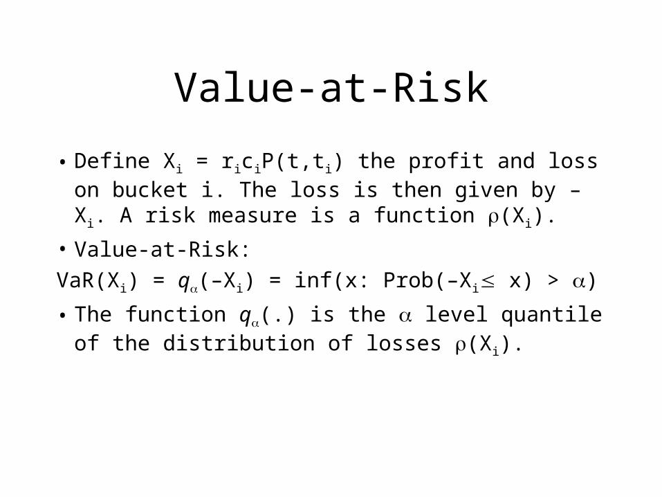
Value-at-Risk

• Define Xi = riciP(t,ti) the profit and loss on bucket i. The loss is then given by –Xi. A risk measure is a function (Xi).

• Value-at-Risk:

VaR(Xi) = q(–Xi) = inf(x: Prob(–Xi x) > )

• The function q(.) is the level quantile of the distribution of losses (Xi).

VaR as “margin”

• Value-at-Risk is the corresponding concept of “margin” in the futures market.

• In futures markets, positions are marked-to-market every day, and for each position a margin (a cash deposit) is posted by both the buyer and the seller, to ensure enough capital is available to absorb the losses within a trading day.

• Likewise, a VaR is the amount of capital allocated to a given risk to absorb losses within a holding period horizon (unwinding period).

VaR as “capital”

• It is easy to see that VaR can also be seen as the amount of capital that must be allocated to a risk position to limit the probability of loss to a given confidence level.

VaR(Xi) = q(–Xi) = inf(x: Prob(–Xi x) > ) = inf(x: Prob(x + Xi > 0) > ) =

= inf(x: Prob(x + Xi 0) 1 – )

VaR and distribution

• Call FX the distribution of Xi. Notice that

• FX(–VaR(Xi)) = Prob(Xi –VaR(Xi))

= Prob(– Xi >VaR(Xi)) = Prob(– Xi > F–X

–1())

= Prob(F–X (– Xi ) > ) = 1 – • So, we may conclude

Prob(Xi –VaR(Xi)) = 1 –

VaR in a parametric approach

• pi marking-to-market of cash flow i

ri, percentage daily change of i-th factor

Xi, profits and losses piri

• Example: ri has normal distribution with mean i and

volatility i, Take = 99%

Prob(ri i – i 2.33) = 1%

If i = 0, Prob(Xi = ri pi – i pi 2.33) = 1%

VaRi = i pi 2.33 = Maximum probable loss (1%)

VaR methodologies

• Parametric: assume profit and losses to be (locally) normally distributed.

• Monte Carlo: assumes the probability distribution to be known, but the pay-off is not linear (i.e options)

• Historical simulation: no assumption about profit and losses distribution.

VaR methodologies• Parametric approach: assume a distribution

conditionally normal (EWMA model ) and is based on volatility and correlation parameters

• Monte Carlo simulation: risk factors scenarios are simulated from a given distributon, the position is revaluated and the empirical distribution of losses is computed

• Historical simulation: risk factors scenarios are simulated from market history, the position is revaluated, and the empirical distribution of losses is computed.

Value-at-Risk criticisms

• The issue of coherent risk measures (aximoatic approach to risk measures)

• Alternative techniques (or complementary): expected shorfall, stress testing.

• Liquidity risk

Coherent risk measures

• In 1999 Artzner, Delbaen-Eber-Heath addressed the following problems

• “Which features must a risk measure have to be considered well defined?”

• Risk measure axioms:  Positive homogeneity: (X) = (X) Translation invariance: (X + ) = (X) –

 Subadditivity: (X1+ X2) (X1) + (X2)

Flaws of VaR

• Value-at-Risk is the quantile corresponding to a probability level.

• Critiques:– VaR does not give any information on the shape of the

distribution of losses in the tail– VaR of two businesses can be super-additive (merging

two businesses, the VaR of the aggregated business may increase

– In general, the problem of finding the optimal portfolio with VaR constraint is extremely complex.

Expected shortfall

• Expected shortfall is the expected loss beyond the VaR level. Notice however that, like VaR, the measure is referred to the distribution of losses.

• Expected shortfall is replacing VaR in many applications, and it is also substituting VaR in regulation (Base III).

• Consider a position X, the extected shortfall is defined as

ES = E(X: X VaR)

Elicitability

• A new concept is elicitability, that means that there exists a function such that one can measure whether a measure is better then another.

• In other words, a measure is elicitable if it results from the optimization of a function. For example, minimizing a quadratic function yields the mean, while minimizing the absolute distance yields the median.

• Surprise: VaR is elicitable, while ES is not. • A new class of measures, both coherent and

eligible? Expectiles!

Economic capital and regulation

• Since the 80s the regulation has focussed on the concept of economic capital, defined as the distance between expected value of an investment and its VaR.

• In Basel II and Basel III the banks are required to post capital in order to face unexpected losses. The capital is measured by VaR

• In Solvency II and Basel IV VaR will be substituted by expected shortfall.

Non normality of returns

• The assumption of normality of of returns is typically not borne out by the data. The reason is evidence of – Asimmetry – Leptokurtosis

• Other casual evidence on non-normality– People make a living on that, so it must exist– If nornal distribution of retruns were normal the crash

of 1987 would have a probability of 10–160, almost zero…

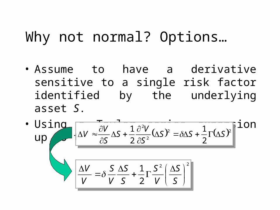
Why not normal? Options…

• Assume to have a derivative sensitive to a single risk factor identified by the underlying asset S.

• Using a Taylor series expansion up to the second order

22

2

2

2

1

2

1SSS

S

VS

S

VV

22

2

2

2

1

2

1SSS

S

VS

S

VV

22

2

1

S

S

V

S

S

S

V

S

V

V 22

2

1

S

S

V

S

S

S

V

S

V

V

Why non-normal? Leverage…

• One possible reason for non normality, particularly for equity and corporate bonds, is leverage.

• Take equity, of a firm whose asset value is V and debt is B. Limited liability implies that at maturity

Equity = max(V(T) – B, 0)• Notice that if at some time t the call option

(equity) is at the money, the return is not normal.

Why not normal? Volatility

• Saying that a distribution is not normal amounts to saying that volatility is constant.

• Non normality may mean that variance either– Does not exist– It is a stochastic variable

Dynamic volatility

• The most usual approach to non normality amounts to assuming that the volatility changes in time. The famous example is represented by GARCH models

ht = + shock2t-1 + ht -1

Arch/Garch extensions

• In standard Arch/Garch models it is assumed that conditional distribution is normal, i.e. H(.) is the normal distribution

• In more advanced applications one may assume that H be nott normally distributed either. For example, it is assumed that it be Student-t or GED (generalised error distribution). Alternatively, one can assume non parametric conditonal distribution (semi-parametric Garch)

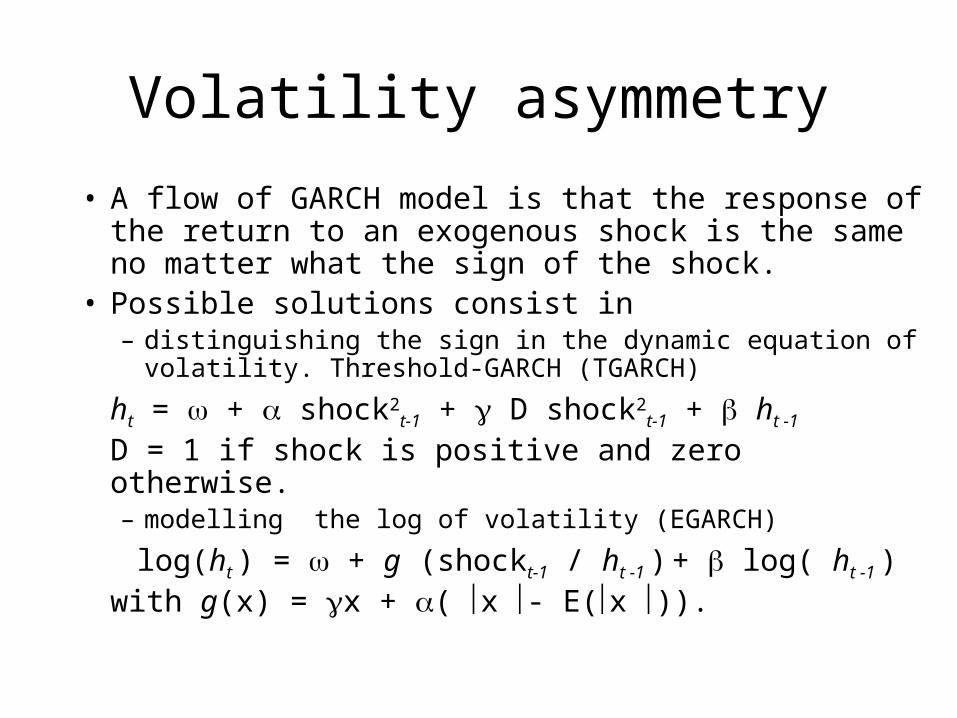
Volatility asymmetry

• A flow of GARCH model is that the response of the return to an exogenous shock is the same no matter what the sign of the shock.

• Possible solutions consist in– distinguishing the sign in the dynamic equation of volatility.

Threshold-GARCH (TGARCH)

ht = + shock2t-1 + D shock2

t-1 + ht -1

D = 1 if shock is positive and zero otherwise.– modelling the log of volatility (EGARCH)

log(ht ) = + g (shockt-1 / ht -1 ) + log( ht -1 )with g(x) = x + ( x - E(x )).

High frequency data

• For some markets high frequency data is available (transaction data or tick-by-tick).– Pros: possibility to analyze the price dynamics

on very small time intervals – Cons: data may be noisy because of

microstructure of financial markets. • “Realised variance”: using intra-day statistics to

represent variance, instead of the daily variation.

Subordinated stochastic processes

• Consider the sequence of log-variation of prices in a given price interval. The cumulated return

R = r1 + r2 +… ri + …+ rN

is a variable that depends on the stoochastic processes

a) log-returns ri.b) the number of transactions N.

• R is a subordinated stochastic process and N is the subordinator. Clark (1973) shows that R is a fat-tail process. Volatility increases when the number of transactions increases, and it is then correlated with volumes.

Stochastic clock

• The fact that the number of transactions induces non normality of returns suggest the possibility to use a variable that, changing the pace of time, could restore normality.

• This variable is called stochastic clock. The technique of time change is nowadays one of the most used tools in mathematical finance.

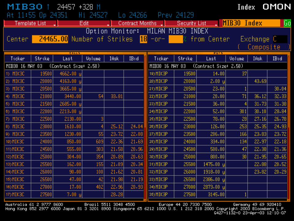
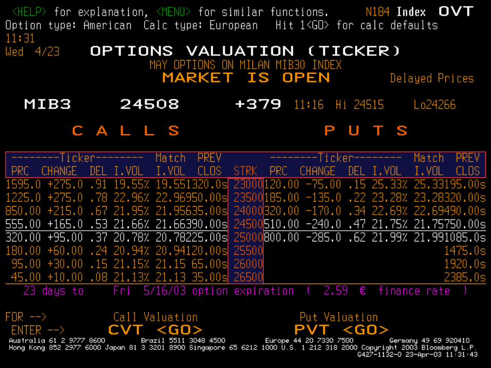
Implied volatility

• The volatility that in the Black and Scholes formula gives the option price observed in the market is called implied volatility.

• Notice that the Black and Scholes model is based on the assumption that volatility is constant.

The Black and Scholes model

• Volatility is constant, which is equivalent to saying that returns are normally distributed

• The replicating portfolios are rebalanced without cost in continuous time, and derivatives can be exactly replicated (complete market)

• Derivatives are not subject to counterpart risk.

Beyond Black & Scholes

• Black & Scholes implies the same volatility for every derivative contract.

• From the 1987 crash, this regularity is not supported by the data– The implied volatility varies across the strikes

(smile effect)– The implied volatility varies across different

maturities (volatility term structure)• The underlying is not log-normally distributed

Smile, please!Smiles in the equity markets

0

0,5

1

1,5

2

2,5

3

3,5

4

0,8 0,85 0,9 0,95 1 1,05 1,1 1,15 1,2 1,25 1,3

Moneyness

Imp

lied

Vo

lati

lity

Mib30

SP500

FTSE

Nikkei

Trading strategies with options

• Trade the skew: betting on a reduction of the skewness = flattening of the smile

• Trade of the fourth moment: betting on a decrease of out and in the money options and increase of the at-the-money options.

• Volatility surface: change of volatility across strike prices and maturities.