Financial Economics

Course requirements What is Finance? Course outline

Financial Economics

Peter Kondor

Fall 2012


Part

Course overview


Outline of Part 0

Course requirements

What is Finance?

Course outline


Contact

Office 404 Nador u. 9.Phone 2206E-mail [email protected] Hours by appointment


Financial Economics

• aim: Cutting edge rsearch in Finance• career objective: PhD/IMF/Central Banks• learn to read/write academic papers• high level maths is needed• main material: academic papers• background in finance is not necessary


• For MA: two finance courses• minimal overlap• different objectives

Investments Financial Economics

aimtheory behind practice

of financial investment

cutting edge

research in Finance

career objective business (public service) PhD / IMF/ Central Banks

”literacy” learn to read WSJ/FT, policy papers learn to read/write academic papers

maths decent, but undergrad level high level

materialstandard text book +

articles from financial pressacademic papers

background in finance? not neccessary not necessary


Course requirements

1. Presentation of a paper• chosen from a menu• 30 minutes• What is the main idea?• Which are the main ingredients?• How does it work?• How does it relate to the material of this course?

2. class participation (10%)3. Final exam (90%)


Basic notions

• What is an asset?• Price vs returns?• stocks/bonds/ contingent claims (derivatives)?• portfolio?• mutual fund/hedge fund?


What is Finance?• Structure of financial markets


• in the language of economics: Asset prices ensure thatsavings equal investment

• allocation of consumption and investment across statesand time

• risk-sharing among individuals• think of: insurance, investments in your pension, saving on

your deposit• has to match: firms production possibilities and decisions• if allocation works well: efficient production


• Two main approaches:• Consumption based asset pricing

• Suppose financial markets work smoothly: Can we build amodel of portfolio choice, which matches the factsquantitatively?

• no frictions: representative agent’s decision on optimalconsumption/investment

• in focus: relationship between aggregate consumption dataand returns of assets

• 60% in academic finance, 10% of this course

• Frictions in financial markets:• What can go wrong on financial markets?• frictions: asymmetric information, search frictions, capital

constraints, bubbles• ”changing liquidity”• 30% in academic finance, 90% of this course


Course outline

I Consumption based asset pricing1. The Euler-equation and classic issues in Finance2. Time series: predictability and the equity premium


II Frictions in financial markets4. Classic mdoels of asset pricing under asymmetric information5. Herding6. Delegated portfolio management7. OTC markets (search and networks)8. Capital constraints and limits to arbitrage9. Bubbles and crashes

10. Collateral requirement and asset prices11. Knightian Uncertainty

The problem Interpretations Classic issues in Finance Consumption based model in practice Alternative approaches

Part I

The Euler equation and the classic issues inFinance


Outline of Part I

The problem

Interpretations

Classic issues in Finance

Consumption based model in practice

Alternative approaches


The problem of the representative investor

• The problem: how much to consume/ how much to invest

maxξ

u(ct ) + βEt [u(ct+1)]

s.t .ct = et −ptξ

ct+1 = et+1 + xt+1ξ

• First-order condition / Euler-equation

ptu′(ct ) = Et [βu′(ct+1)xt+1]

pt = Et [βu′(ct+1)

u′(ct )xt+1]


Interpretations of the Euler condition

• rewrite Euler as

pt = Et [mt+1xt+1]

mt+1 = βu′(ct+1)

u′(ct )

• or p = E [mx ]

• m is the pricing kernel• prices any claim (as we will see)• for example: risk free rate• xt+1 = Rt ,pt = 1

Rt =1

Et [mt+1]


• m also determines the stochastic discount factor• suppose an asset paying the random dt in each t• problem in infinite time

max{ξj}∞

j=t

Et

[∞

∑j=0

βju(ct+j

)]ct = et −ξtpt

ct+j = dt+j

t+j−1

∑k=t

ξk + et+j −ξt+jpt+j for all j > 0


• from first order condition

pt+j = Et

(∞

∑k=t+j

βk−t u′ (ck+1)

u′ (ck )dk+1

)= Et

(∞

∑k=t+j

mt ,k+1dk+1

)

• Note that mt ,k+1 works as a discount factor (but it isstochastic, hence the name)

• check that this implies

pt = Et (mt+1 (pt+1 + dt+1))

• same condition as before


• m also determines the state price density• consider S states indexed by s = 1,2... and corresponding

Arrow-Debreu securities• if the price of the A-D security is pc(s) in state s, then the

price of our asset with pay-off x(s) must be

p =S

∑s=1

pc(s)x(s)

• ”Happy-meal theorem” (Cochrane)


• or

p =S

∑s=1

π (s)pc (s)

π (s)x (s) =

S

∑s=1

π (s)m (s)x (s) = E (mx)

• π(s)m(s) is the state-price density• transformed state-price


• m also determines risk-neutral probabilities• define risk neutral probabilities

π∗ (s)≡ m (s)

E (m)π (s) = Rf m (s)π (s)

• check that this implies

p =1

Rf

S

∑s=1

π∗ (s)x (s) =

1Rf E∗ (x)

• where we took expectations under the new probabilities• adjust probabilities to take into account the ”importance” of

the event• basis of risk-neutral pricing• extensively used on Wall Street to price derivatives


Classic issues in Finance: The risk free rate

• suppose no uncertainty in consumption growth• suppose CRRA utility:

u(c) =c1−γ

1− γ

• if no uncertainty in consumption growth thenRf = 1/E(m) = 1/Et [β (ct+1

ct)−γ ] implies

Rf =1β

(ct+1

ct)γ

• Risk free rate increases in...


• suppose consumption is lognormally distributed andr ft ≡ lnRf

t , δ ≡− lnβ

• using

E (ez) = eE(z)+ var(z)2

• gives

Rft =

[e−δ e−γEt (∆ lnct+1)+

γ2var(∆ lnct+1)2

]−1


• taking logarithm

r ft = δ + γEt (∆ lnct+1)− γ2var (∆ lnct+1)

2• similar comparative statics plus precautionary savings• can do the argument backwards: consumption growth

varies with the risk free rate• particulars of the CRRA: γ substitution across time, across

states, precautionary savings


Classic issues: Risk correction

• Let us turn to risky assets• Remember

cov(m,x)≡ E(mx)−E(m)E(x)

• Thus, p = E(mx) implies

p = E(m)E(x) + cov(m,x) =E(x)

Rf + cov(m,x)

• present value + risk adjustment


•

p =E(x)

Rf + cov(βu′(ct+1)

u′(ct ),xt+1)

• which asset has a high price?• why? (think about insurance)• why covariance and not variance?• idea: add a little (ξ ) to your portfolio, it has only

second-order effect on your consumption stream

σ2(c + ξx) = σ

2(c) + 2ξcov(c,x) + ξ2σ

2(x)


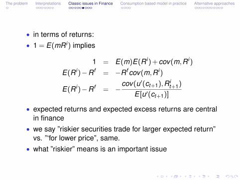
• in terms of returns:• 1 = E(mR i) implies

1 = E(m)E(R i) + cov(m,R i)

E(R i)−Rf = −Rf cov(m,R i)

E(R i)−Rf = −cov(u′(ct+1),R i

t+1)

E [u′(ct+1)]

• expected returns and expected excess returns are centralin finance

• we say ”riskier securities trade for larger expected return”vs. ”‘for lower price”, same.

• what ”riskier” means is an important issue


Classic issues: Expected Return-Beta Representation

• write the previous equation as

E(R i) = Rf +cov(m,R i)

var(m)(−var(m)

E(m))

E(R i) = Rf + βi ,mλm

• expected return=risk free rate+quantity of risk x price ofrisk

• β : regression coefficient of asset return on discount factor,asset specific,

• λ is market specific• one-factor model• how to get λ?


• assuming CRRA, lognormal consumption growth andtaking Taylor approximation (for small variance, problem1/5)

•

E(R i) = Rf + βi ,∆cλ∆c

λ∆c = γvar(∆c)

• expected return should increase linearly in consumptiongrowth

• λ depends on risk aversion and volatility of consumption• returns are larger if risk aversion is larger, or environment

is more volatile


Classic issues: idiosyncratic risk does not effect prices

• large variance, large return?• only risk correlated with m gets compensation: if

cov(m,x) = 0 then p = E(x)Rf

• decompose payoff as

x = proj(x |m) + ε

• no compensation for ε part as E(mε) = 0 by definition• the compensation for x is the same as the compensation

for x = proj(x |m)


Consumption based model in practice

• let us take the Euler-condition seriously• suppose that the representative agent solves our problem

with utility

u(c) =c1−γ

1− γ

• then m = β (ct+1ct

)γ thus any excess return has to obey

0 = Et [β (ct+1

ct)−γRe

t+1]

• orEt [Re

t+1] =−Rf cov(β (ct+1

ct)−γ ,Re

t+1]


• we have data on aggregate consumption and we have dataon returns. We can calculate the covariance on the lefthand side

• it should work for any asset (stocks, bonds, options)• Does returns line up with any γ?


Something is wrong


Something is wrong

• there is positive correlation• but pricing errors are same order of magnitude as the

spread across portfolios• also, risk aversion is too large


Alternative approaches

1. Different utility functions• nonseparabilities (stock of durable goods, past

consumption affects marginal utility)• micro data on individual consumption (cross-sectional

variance of income)• (more on this in next part)


2. Factor pricing models• connect pricing kernel directly to factors which we can

measure better• a significant part of the literature (Fama-French factors and

alike), but we have to skip this


3. General equilibrium models• we could close our economy• let us model the decision rule ct = f (yt , it ...)• we can connect pricing kernel or beta to other variables• perhaps, consumption data is bad• when you want to close the economy, without the

complications: Lucas’s asset-pricing model (Lucas, 1978)


The Lucas-tree model

• endowment economy:• large number of identical agents with log preferences• only durable good: a set of identical trees (”Lucas-tree”),

one for each person in the economy• at the beginning of each period tree gives a stochastic,

perishable fruit dt (aggregate risk)• fruit follows a Markov process: dt = ds,s = 1, ...S• one share per tree is traded, each agent starts with one tree• representative agent is fine• bonds are in zero-net supply


• problem with ξ shares and ψ bonds

V (ws) = maxξ ,ψ

u (cs) + βE(V(w ′s′))

w ′s′ = ξ (ds′ + ps′) + ψRs

ws = cs + ξps + ψ

• or

V (ws) = maxξ ,ψ

u (ws− (ξps + ψ))+βE (V (ξ (ds′ + ps′) + ψRs))


• The first order conditions are

u′ (cs)ps = βE(

V ′w ′s (ds′ + ps′))

u′ (cs) = βE(

V ′w ′sRs

)• and the envelope condition is

V ′ws(ws) = u′ (cs)


• giving

u′ (cs)ps = βE(u′ (cs′)(ds′ + ps′)

)u′ (cs) = βE

(u′ (cs′)Rs

)• with logarithmic utility and market clearing cs = ds

ps =β

1−βds

• note that price dividend ratio is constant across states


• In finance, it is more common to use the Mehra-Prescott(1985) version (this is the famous equity premium puzzlepaper)

• modify that growth rate of dt follows a markov process• that is dt

dt−1changes across λs,s = 1, ...,S and utility is

CRRA


u′ (dt )pt = βE(u′ (dt+1)(dt+1 + pt+1)

)pt

dt= βE

((dt

dt+1

)γ(dt+1

dt+

pt+1

dt

))pt

dt= βE

((dt

dt+1

)γ dt+1

dt

(1 +

pt+1

dt+1

))pt

dt= β

S

∑s=1

πss′ (λs′)1−γ

(1 +

pt+1

dt+1

)pds = β

S

∑s=1

πss′ (λs′)1−γ (1 + pds′)

• solve for price-dividend ratios in different states


• from price-dividend ratios returns are

Rss′ =ps′ + ds′

ps=

ds′

ds

ps′/ds′ + ds′

ps/ds=

= λs′pds′ + 1

pds

• why does this version fit better for calibration?


• In these versions production is not influenced byinvestment

• endowment economy• more sophisticated general equlibrium models include full

blown production functions• RBC models with twists:

• Jermann (1998), Boldrin, Chirstiano, and Fisher (2001)

Predictability and excess volatility The equity premium New models Lessons

Part II

Time series: predictability and the equitypremium


Outline of Part II

Predictability and excess volatility

The equity premium

New models

Lessons


Euler-equation and the time-series• pick one asset (e.g. market portfolio)• remember:

ptu′(ct ) = Et [βu′(ct+1)(pt+1 + dt+1)]

• if investors were risk-neutral or there were no variation inconsumption, no dividends, and β = 1, then Et (pt+1) = pt

• best predictor for future price is current price, prices aremartingales, they follow a random walk

• under the more general conditions: prices are martingalesif we adjust for dividends and scale by the marginal utility(remember: risk-neutral probabilities)

• random walk idea is a good approximation for day-to-daychanges (β close to one, consumption does not change)

• thus, technical analysis/systems/newspaper advice doesnot generate profit


• But: evidence that long-horizon excess returns are quitepredictable

• write

Et [Rt+1]−Rft =−covt (mt+1,Rt+1

Et [mt+1]=

=−σ(mt+1)

Et [mt+1]σt (Rt+1)ρt (mt+1,Rt+1)

≈ γtσt (∆ct+1)σt (Rt+1)ρt (mt+1,Rt+1)

• subscript of t :conditional on today’s information set: weshould have written it everywhere (we skipped it to simplifynotation only)


• possibilities1. conditional variance over return changes over time (does

not help too much in the data2. conditional correlation does not look very promising3. changing risk, σt (∆ct+1)4. changing risk aversion, γt

• think about the business cycle


Price to dividend ratio and returns


Predictability in the data

• in 1 year, not very impressive• but for longer periods, gets stronger• any similar ratios would work: earnings to price, current

price to moving average of past prices• many other variables forecast returns: term-spread long

and short bonds, default spread, investment/capital,consumption/wealth

• correlated with each other, correlated or forecast businesscycles

• expected returns change over the cycle


• persistence of d/p, small predictability in the short-termand large predictability on the long term are consistent

• think of: forecasting the weather overnight,forecasting itthrough 3 months

• estimates are consistent with small values of b,R2 andlarge values of ρ in

rt+1 = bxt + εt+1

xt+1 = ρxt + δt+1

• we are not ”increasing power” through increasing the termof the forecast


• also means that forecastability relies on few observations• high d/p in the 50s preceded the boom in the 60s• low d/p in the 60s preceded the poor returns in 70s• high d/p in mid-70s preceded the boom in 90s• three postwar data points• in 1990s d/p decrease but high returns, regression

coefficient is cut half• current downturn definitely helps


Time-series of e/p and 5-year ahead returnsChart4

Page 1

-0.1

-0.05

0

0.05

0.1

0.15

0.2

0.25

1945

1950

1955

1960

1965

1970

1975

1980

1985

1990

1995

2000

2005

2010

0

0.02

0.04

0.06

0.08

0.1

0.12

0.14

0.16

5-year returnE/P


Volatility


• Shiller (1981): huge volatility of prices compared todiscounted stream of dividends

• typical year 16% change in stock prices, 30% is notuncommon

• many times no apparent news• ”Thirty percent of capital stock of US vanished and no one

noticed?”• connected to predictability: too low prices today implies too

high returns in the future: as prices rebound to their correctlevel


• we will see that if prices are high relative to dividends theneither

1. investors expect dividends to rise2. investors expect returns to fall3. (investors expect prices to rise forever)

• it comes from an identity• Historically, virtually all variation comes from (2), varying

excess returns


• observe that

1 = R−1t+1Rt+1 = R−1

t+1Pt+1 + Dt+1

Pt

Pt

Dt= R−1

t+1

(1 +

Pt+1

Dt+1

)Dt+1

Dt

Pt

Dt= R−1

t+1

(1 + R−1

t+2

(1 +

Pt+2

Dt+2

)Dt+2

Dt+1

)Dt+1

Dt

Pt

Dt= Et

∞

∑j=1

j

∏k=1

R−1t+k

Dt+k

Dt+k−1

• high prices must come from high future dividend growth orlow future returns

• which is it?


• to get a linear version which we can easily estimate westart by taking logs of the second equation and taking theTaylor-expansion of ln(1 + ex ) around P/D = ep−d ,

pt −dt =−rt+1 + ∆dt+1 + ln(1 + ept+1−dt+1)

≈−rt+1 +∆dt+1 + ln(1+P/D)+P/D

1 + P/D[pt+1−dt+1−(p−d)]

=−rt+1 + ∆dt+1 + k + ρ(pt+1−dt+1)

= const +∞

∑j=1

ρj−1(∆dt+j − rt+j)

= const + Et [∞

∑j=1

ρj−1(∆dt+j − rt+j)]


• the one but last result implies (taking covariance withpt −dt )

var(pt −dt ) = cov(pt −dt ,∞

∑j=1

ρj−1(∆dt+j))

−cov(pt −dt ,∞

∑j=1

ρj−1(rt+j))

• right hand side are exponentially weighted numerators ofregression coefficients

• P/D can only vary if they forecast either dividend growth orreturns (or both)


Volatility decomposition


• estimate shows that high prices forecast lower dividendgrowth

• they forecast really low returns, variation in returns accountfor more than 100%

• forecasting power is not extremely strong, but we know thatit has to forecast one of them: choice is obvious

• Vuolteenaho (1999) did the same analysis to firms:• half of the variation in individual D/P is due to variation in

future cash flows• most of the cash flow variation is idiosyncratic• hence, in the index it washes out, and all that left is varying

expected returns


The equity premium puzzle

• upper bound on Sharpe-ratio

1 = E(

mR i)

= E (m)E(

R i)

+ ρm,R i σ

(R i)

σ (m)

E(

R i)

= Rf −ρm,R iσ(m)

E(m)σ(R i)

• observing that∥∥ρm,R i

∥∥≤ 1 gives∥∥∥∥∥E(R i)−Rf

σ(R i) ∥∥∥∥∥≤ σ(m)

E(m)


• Left hand side is Sharpe-ratio: return-per-risk, better thanreturn, you cannot improve it just by increasing yourleverage (borrowing a dollar and investing in the asset)

• for any frontier return the Sharpe-ratio or the slope of thefrontier: ∥∥∥∥E(Rmv )−Rf

σ (Rmv )

∥∥∥∥=σ(m)

E(m)= σ(m)Rf

• depends on the volatility of the discount factor


• with CRRA utility and lognormal consumption growth∥∥∥∥E(Rmv )−Rf

σ (Rmv )

∥∥∥∥=σ [(ct+1/ct )

−γ ]

E [(ct+1/ct )−γ ]

=√

eγ2σ2(∆ lnct+1)−1≈ γσ(∆ lnc)

• right hand side is large if consumption is volatile or riskaversion is large


• in the postwar U.S. data, the slope of the historicalmean-standard deviation frontier is much higher thanreasonable risk-aversion would suggest

• real stock returns: 9%• standard deviation of real returns: 16%• real returns on bonds: 1%• thus, Sharpe-ratio about 0.5• aggregate nondurable and services consumption mean

and standard deviation: 1%• for this, you need γ = 50, way too large• or, a log-utility investor should invest much more in the

stock market, to have a volatility of consumption of 50%


• Theoretically either1. people are much more risk-averse than we think or2. stock returns of last 50 years are due to good luck and not

compensation or3. something is wrong with the model (utility function,

aggregate consumption data)


• What is the problem with high risk aversion?• remember that

1/Rft = Et [mt+1] = Et [β

(Ct+1

Ct

)−γ

]

• large γ implies very large risk free rate• idea: very large risk aversion implies that they are unwilling

to substitute today’s consumption by tomorrow’sconsumption

• intertemporal elasticity of substitution is very large• shows: probably we want to separate preferences across

states, from preferences across time


Basic ideas

1. individual shocks• abandon representative agent assumption: uninsurable

individual income shocks implies more volatile individualconsumption than aggregate

• problem: might not be enough (you would need variance ofindividual consumption of 50%-250% and it is not durables)

• individual consumption growth will be less correlated withstock returns (the more it varies, the less is the correlation)


2. Luck• standard deviation of stock returns is very high• using σ/

√T , standard error for 50 years is 2.3% which

gives a 2-s.e. confidence interval for the equity premium of3% - 13%

• this could go either way• many argues (Brown,Goetzmann and Ross, 1995) that U.S.

data suffers selection bias: U.S. was lucky in the last50-100 years


• Campbell (1999) checks for other countries which there isdata for 1970-1995, but finds the same premium than U.S.

• However, other countries are Canada, Japan, Australia andWestern Europe: probably same luck

• we should check countries with less luck: Russia, LatinAmerica, Germany and Japan through wars, China etc

• but there is no data exactly because of the interruptions ofwars, revolutions etc.

• Fundamental question: Did investors in 1947 anticipate 8%equity premium and still did not invest?

• or was it a surprise? (the first is the equity premium)• However, even 3% equity premium is hard to explain


3. Rare disasters• Rietz (1988): small probability but large disasters can

explain the puzzle e.g. Great Depression, Wars• We rarely observe them, but average investor needs

compensation for them• Recently, renewed debate started by Barro (2005) and

followed by Gabaix (2007), Gosh and Julliard (2008), Martin(2008)


• Barro’s exercise:• Mehra-Prescott version of Lucas’s asset pricing model• dividend

logdt+1 = logdt + γ + ut+1 + vt+1

• γ ≥ 0• with probability e−p, vt+1 = 0• with probability 1−e−p, vt+1 = log(1−b) < 0• calibrate b,p from data of 20 OECD countries, GDP fall of

more than 15% during an event (not a year)• argues that rare disasters can explain equity premium


• many think that Barro’s calibration is wrong, e.g. Gosh andJuillard (2008):

• calibrates a yearly model using the cumulated multi-yearcontraction observed during disasters

• he assumes that the consumption drop during disasters isequal to the contraction in GDP.

• Gosh and Juillard argue that it is unlikely that disasters canwork

• Martin (2008) argues that a model with rare disasters isnecessarily very sensitive to calibration


New models

• coming up with a model which generates large equitypremium is not enough

• if it is the right model, it should account for all (most)stylized facts:

• high Sharpe-Ratio of market portfolio• high volatility of stock returns• low and relatively constant interest rates• i.i.d. consumption growth with small volatility• predictability: low prices compared to dividends today imply

high excess returns• cross-sectional variation in expected returns• time-varying volatility of stock returns• with reasonable risk-aversion


Campbell-Cochrane’s habit formation

• How to make the representative agent more risk-averse ina recession?

• by giving them habits: large marginal utility whenconsumption is low relative to trend

• instead of internal: getting used to consumption• they pick external: “Keeping up with the Joneses”


Model• consumption: δct+1 = g + vt+1• utility:

E

[∞

∑0

δt (Ct −Xt )

1−γ −11− γ

]• intuitively habit should do: xt = φxt−1 + λct , but that is too

messy• so, instead surplus consumption ratio follows something

like AR(1)

St =Ct = Xt

Ct

st+1 = (1−φ)s + φst + λst (ct+1−ct −g) (1)

• consumption is always above habit• also λ (s) = 1

S

√1−2(st − s)−1

• St is state variable• marginal utility is (StCt )

−γ

Marginal Utility

1. Marginal Utility with external habit

Mt+1 ≡ δuc (Ct+1,Xt+1)

uc (Ct ,Xt )=(

St+1

St

Ct+1

Ct)−γ

2. The local curvature of the utility function is related to the surplusconsumption ratio:

ηt ≡ −Ctucc (Ct ,Xt )uc (Ct ,Xt )

= γSt

Thus low consumption relative to habit (or a low surplus consumptionratio) implies a high local curvature of the utility function.

6 / 16

The risk free rate

1. Calculating the risk-free rate assuming lognormality of consumption growth

r ft = −ln(δ) + γg − γ(1− φ)(st − s)− λ2σ2

2[1 + λ(st)]2

The third term in the eq. reflects intertemporal substitution: if cons. islow relative to habit (eg. in recession) then consumers borrow which drivesup the interest rate. The last term is reflects the precautionary savingseffect: as uncertainty increases consumers are more willing to save whichdrives down the interest rate. Thus, the relatively constant risk-freeinterest rate is sustained.

2. The functional form choosen for λ(st) has to offset the two forcesmentioned before.

3. The habit model allows high ”risk aversion” with ”aversion tointertemporal substitution” and it is consistent with consumption andinterest rate data.

7 / 16

The Sharpe ratio

1. The Sharpe ratio is coming from the FOC, 0 = Et(Mt+1Ret+1), for an

excess return Ret+1:

Et (r)−r ft

σt (r)=ηtσtcorr(∆c, r)

2. High curvature,ηt , means that the model can explain the equity premium.Curvature ηt that varies over time as consumption rises in booms and fallstoward habit in recessions means that the model can explain atime-varying and countercyclical Sharpe-ratio, despite constantconsumption volatility, σt(∆c) and correlation corrt(∆c, r).

8 / 16

Pricing a consumption claim

1. Modelling stocks as a claim to the consumption stream:PtCt

(st)=Et [Mt+1Ct+1

Ct[1 +

Pt+1

Ct+1(st+1)]]

The surplus-consumption ratio st is the only state variable for theeconomy, so the price/consumption ratio is a function only of st .

2. Solution to this eq: We substitute for Mt+1 and consumption growth andsolve this functional eq. numerically on a grid for st using numericalintegration over the normally distributed shock vt+1.

3. We assume that there is an endowment process for the dividend growth.U.S. data suggests that consumption and stock market dividends areweakly correlated. Therefore it is crucial to model the dividends andconsumption separately. But there is some correlation betweenconsumption and dividend growth rates.

∆dt+1 = g + wt+1, wt+1 ∼ i .i .d .N(0, σ2w ), corr(wt , vt) = ρ

4. Calculating the price/dividend ratio is through the same eq. as above(instead of Ct we have Dt and the same solution method.)

9 / 16

Price Dividend ratio as a function of surplus-consumption ratio

10 / 16

Conditional Moments of Returns-Expected Return and the Risk-free Rate

11 / 16


Parameters in CC


Results in CC


Lessons from Consumption Based Asset Pricing

• assets are useful because they transfer our dollars acrossstates and time

• the valuation of an investor depends on her valuation of adollar across different states and time

• this information is summarized by the pricing kernel• target: have a simple model which validates this

relationship• seems that pricing kernel from standard utility functions

and with aggregate consumption does not do a good job


• in time-series• expected return is higher in recessions: marginal utility

increases more than validated by smaller consumption• consumption is too smooth• seems we need state-dependent marginal utility of some

type (habits, Epstein-Zin and long-run risk, idiosyncraticrisk)

Financial Economics

Documents

Transcript of Financial Economics