Final Report Submitted to the on
166
Final Report Submitted to the Second Strategic Highway Research Program (SHRP 2) on L38 Pilot Testing of SHRP 2 Reliability Data and Analytical Products Submitted by Washington State Department of Transportation In Association with: Smart Transportation Applications and Research Laboratory (STAR Lab) University of Washington July 30, 2014
Transcript of Final Report Submitted to the on
Final Report
Submitted to the
Second Strategic Highway Research Program
(SHRP 2)
on
L38
Pilot Testing of SHRP 2
Reliability Data and Analytical Products
Submitted by
Washington State Department of Transportation
In Association with:
Smart Transportation Applications and Research Laboratory (STAR Lab)
University of Washington
July 30, 2014

SHRP 2 Project L38D, WSDOT – University of Washington Final Research Report
Page II
ACKNOWLEDGMENT OF SPONSORSHIP
This work was sponsored by Federal Highway Administration in cooperation with the American
Association of State Highway and Transportation Officials, and it was conducted in the Second
Strategic Highway Research Program, which is administered by the Transportation Research
Board of the National Academies.
DISCLAIMER
This is an uncorrected draft as submitted by the research agency. The opinions and conclusions
expressed or implied in the report are those of the research agency. They are not necessarily those
of the Transportation Research Board, the National Academies, or the program sponsors.

SHRP 2 Project L38D, WSDOT – University of Washington Final Research Report
Page III
AUTHORS
John Nisbet, Daniela Bremmer, Shuming Yan, and Delwar Murshed
Washington State Department of Transportation
Yinhai Wang, Yajie Zou, Wenbo Zhu, Matthew Dunlap, Benjamin Wright, Tao Zhu, and Yingying
Zhang
University of Washington

Page I
Table of Contents
Final Report .................................................................................................................................... I
Table of Contents ........................................................................................................................... I
List of Figures .............................................................................................................................. IV
Executive Summary ................................................................................................................. VIII
Chapter 1 Introduction................................................................................................................. 1
1.1 General Background ........................................................................................................................... 1
1.2 Introduction of SHRP 2 Reliability Data and Analytical Products ..................................................... 2
1.3 Research Objectives .......................................................................................................................... 11
1.4 Final Report Organization ................................................................................................................. 11
Chapter 2 Research Approach .................................................................................................. 12
2.1 Steering Committee .......................................................................................................................... 12
2.2 Test Procedure .................................................................................................................................. 12
2.2.1 Methods or Procedure Testing .................................................................................................. 12
2.2.2 Computer Tool Testing ............................................................................................................... 14
2.2.3 Result Analysis and Feedback .................................................................................................... 15
Chapter 3 Data Compilation and Integration .......................................................................... 17
3.1 Test Site Selection ............................................................................................................................. 17
3.2 Dataset Creation ................................................................................................................................ 18
3.3 Data Quality Control ......................................................................................................................... 30
3.3.1 Loop Detector DQC Procedure................................................................................................... 30
3.3.2 ITS DQC Procedure ..................................................................................................................... 33
3.4 Speed and Travel Time Calculations ................................................................................................. 34
3.4.1 A Travel-Based Approach to Calculating Travel Time from Single Loop Detector Data ............ 35
3.4.2 Calculation of Free-Flow Speed ................................................................................................. 37
3.5 Final Dataset for Analysis .................................................................................................................. 37
3.6 Data Acquisition and Integration ...................................................................................................... 39
Chapter 4 Pilot Testing and Analysis on SHRP 2 L02 Product ............................................. 42

SHRP 2 Project L38D, WSDOT – University of Washington Final Research Report
Page II
4.1 Introduction ...................................................................................................................................... 42
4.2 Test Sites ........................................................................................................................................... 42
4.3 Data Description ............................................................................................................................... 44
4.4 Regime Characterization ................................................................................................................... 44
4.5 Testing Results and Discussion ......................................................................................................... 45
4.6 Practical Applications of the L02 Methodology ................................................................................ 54
4.7 Evaluation of the L02 Objectives ...................................................................................................... 59
Chapter 5 Pilot Testing and Analysis on SHRP 2 L05 Product ............................................. 61
5.1 Introduction ...................................................................................................................................... 61
5.2 SHRP 2 L01/L06 Early Implementation Project ................................................................................. 62
5.3 SHRP 2 L05 Project Comments.......................................................................................................... 63
Chapter 6 Pilot Testing and Analysis on SHRP 2 L07 Product ............................................. 65
6.1 Tool Introduction and Interface ........................................................................................................ 65
6.2 Tool Operability................................................................................................................................. 66
6.3 Tool Usability..................................................................................................................................... 68
6.4 Performance Test .............................................................................................................................. 72
6.5 Test Conclusions................................................................................................................................ 82
Chapter 7 Pilot Testing and Analysis on SHRP 2 L08 Product ............................................. 84
7.1 Introduction ...................................................................................................................................... 84
7.2 Tool Operability................................................................................................................................. 85
7.3 FREEVAL Introduction and Interface ................................................................................................. 86
7.4 Performance Test for FREEVAL ......................................................................................................... 90
7.5 Precision Testing for FREEVAL ........................................................................................................... 97
7.6 Test Conclusions for FREEVAL ........................................................................................................... 98
7.7 STREETVAL Introduction and Interface ............................................................................................. 98
7.8 Input Data Requirements for STREETVAL ....................................................................................... 109
7.9 Performance Test for STREETVAL ................................................................................................... 111
7.10 Test Conclusion for STREETVAL..................................................................................................... 123
Chapter 8 Pilot Testing and Analysis on SHRP 2 C11 Product ........................................... 125
8.1 Introduction .................................................................................................................................... 125
8.2 Description of the Test Site ............................................................................................................. 125
SHRP 2 Project L38D, WSDOT – University of Washington Final Research Report
Page III
8.3 Alternatives to Test ......................................................................................................................... 127
8.4 Input Data ....................................................................................................................................... 128
8.5 Output Data .................................................................................................................................... 129
8.6 Cost of Alternatives ......................................................................................................................... 132
8.7 Benefit-Cost Analysis ...................................................................................................................... 134
8.8 Validation of Outputs from the Travel Time Reliability Tool .......................................................... 136
8.9 Assessment of the Travel Time Reliability Tool .............................................................................. 138
8.10 General Observations ................................................................................................................... 139
8.11 Applicability ................................................................................................................................... 140
Chapter 9 Conclusions and Potential Improvements ............................................................ 142
9.1 Summary and Conclusions .............................................................................................................. 142
9.2 Suggestions and Potential Improvements ...................................................................................... 144
9.2.1 Potential Improvements on SHRP 2 L02 Product .................................................................... 144
9.2.2 Potential Improvements on SHRP 2 L07 Product .................................................................... 145
9.2.3 Potential Improvements on SHRP 2 L08 Product .................................................................... 146
9.2.4 Potential Improvements on SHRP 2 C11 Product .................................................................... 147
9.3 Future Works .................................................................................................................................. 149
References .................................................................................................................................. 151
SHRP 2 Project L38D, WSDOT – University of Washington Final Research Report
Page IV
List of Figures
Figure 2-1 General Approach for Pilot Testing of the SHRP 2 L38 Products ............................. 13
Figure 3-1 Loop detectors in Northwest Washington State .......................................................... 23
Figure 3-2 Traffic Flow Map Based on Loop Detector Data........................................................ 24
Figure 3-3 Traffic Detectors along the SR-522 Corridor .............................................................. 24
Figure 3-4: ALPR Cameras Mounted at the 61st and SR 522 Intersection .................................. 25
Figure 3-5 Traffic Speed Map Based on INRIX Data .................................................................. 27
Figure 3-6 Loop Data Quality Control Flow Chart (Wang et al. 2013) ....................................... 31
Figure 3-7 GUI for Freeway Data Quality Control ...................................................................... 34
Figure 3-9 DRIVE Net Interface with Color-Coded Traffic Flow Feed from WSDOT .............. 40
Figure 3-10 Data Acquisition Methods for the DRIVE Net System (Wang et al., 2013) ............ 41
Figure 4-1 Map of (a) Test Site A (I-5 Facility) and (b) Test Site B (I-405 Facility) .................. 43
Figure 4-2 Travel time index CDFs For All Test Facilities (a) I-5 North; (b) I-5 South; (c) I-405
North; (d) I-405 South. ................................................................................................................. 47
Figure 4-3 Relative Frequency of Each Regime on I-405 North .................................................. 48
Figure 4-4 Relative Contribution of Each Regime to Travel Delay on I-405 North .................... 49
Figure 4-5 Average Travel Delay for Each Regime on I-405 North ............................................ 50
Figure 4-6 Design and Layout of I-405 Braided Ramps Project .................................................. 51
Figure 4-7 Before and After TTI CDF for I-405 Braided Ramp Project under Normal Conditions
....................................................................................................................................................... 52
Figure 4-8 Before and After TTI CDF for I-405 Braided Ramp Project under Incident Conditions
....................................................................................................................................................... 53
Figure 4-9: TTI Standard Deviations for Each Regime Before and After I-405 Ramp Project ... 54
Figure 4-10 DRIVE Net Architecture (Wang et al., 2013) ........................................................... 56
Figure 4-11 Routes Available on the DRIVE Net Platform for L02 Reliability Analysis ........... 57
Figure 4-12: Travel Times for Varying Levels of Reliability for a Custom Route ...................... 58
Figure 4-13: Travel Distance with Varying Levels of Reliability ................................................ 59
Figure 6-1 SHRP 2 L07 Product Interface .................................................................................... 65
Figure 6-2 Warning Dialog for the 64-bit Windows 8 ................................................................. 67
Figure 6-3 Warning Dialog for the OS X 10.6.8 operation system .............................................. 67
SHRP 2 Project L38D, WSDOT – University of Washington Final Research Report
Page V
Figure 6-4 Warning Dialog for Windows 7 .................................................................................. 67
Figure 6-5 HCM 2010 Suggested Default Values for Heavy Vehicles Percentage for Highways68
Figure 6-6 HCM 2010 Suggested Default Values for Trucks and RVs Percentage for Freeways 69
Figure 6-7 Example Movable Cable Median Barrier ................................................................... 70
Figure 6-8 Suggested Thresholds for Movable Cable Median Barrier Treatment ....................... 70
Figure 6-9 Suggested Default Coefficients in L07 Guide ............................................................ 71
Figure 6-10 Output of DRVIE Net system and L07 tool .............................................................. 73
Figure 6-11 Traffic Volume for the Studied Site .......................................................................... 74
Figure 6-12 Comparison of Outputs from Single Loop Detector Data and L07 Tool .................. 75
Figure 6-13 Testing Procedure for L07 ........................................................................................ 76
Figure 6-14 Test site Location for L07 ......................................................................................... 77
Figure 6-15 Traffic Demand Before and After the Treatment ...................................................... 78
Figure 6-16 L07 Tool Crash When Inputting Crash Reduction Percentage ................................. 80
Figure 6-17 L07 Tool Otutput for Benefit-Cost Analysis ............................................................ 81
Figure 6-18 L07 Tool Output for TTI Analysis ............................................................................ 81
Figure 7-1 Methodology Components in SHRP 2 L08 (Kittelson and Associates, Inc., 2013) ... 84
Figure 7-2 Compilation Error Message for Windows 8 Test for STREETVAL .......................... 85
Figure 7-3 FREEVAL Segment Number Selection ...................................................................... 87
Figure 7-4 FREEVAL Ramp Metering Option Selection ............................................................. 88
Figure 7-5 FREEVAL Demand Multiplier ................................................................................... 89
Figure 7-6: Map of Two Study Locations (Pin located at Northgate Mall).................................. 91
Figure 7-7 Sample of Dual Loop Data on I-405 ........................................................................... 93
Figure 7-8 Distribution of Travel Times for I-405 Study Site ...................................................... 93
Figure 7-9 Comparison of Cumulative Distributions for TTI on I-405 ........................................ 94
Figure 7-10 Distribution of Travel Times for I-5 Study Site ........................................................ 95
Figure 7-11 Comparison of Cumulative Distributions for TTI on I-5 .......................................... 96
Figure 7-12 Comparison of Cumulative Distributions for TTI on Differet Seed Days ................ 97
Figure 7-14 Urban Streets Computation Engine (USCE). .......................................................... 102
Figure 7-15 STREETVAL Segment Schematic ......................................................................... 102
Figure 7-16 USRE 2010 HCM ................................................................................................... 103
Figure 7-17 Principal Inputs for Scenario Generation ................................................................ 104
SHRP 2 Project L38D, WSDOT – University of Washington Final Research Report
Page VI
Figure 7-18 Random seed numbers and PHF ............................................................................. 105
Figure 7-19 STREETVAL Scenario Generation ........................................................................ 106
Figure 7-20 Tool Testing Results .............................................................................................. 107
Figure 7-21 Tool results: List of Performance measures for each evaluated scenario ............... 108
Figure 7-22 Distracting floating numbers ................................................................................... 108
Figure 7-23 Malfunctioning Button circled in red ...................................................................... 109
Figure 7-24 Study site location along SR 522, Kenmore, WA. .................................................. 112
Figure 7-25 Study Site Location ................................................................................................. 113
Figure 7-26 Camera Captured Images of Studied Intersections ................................................. 117
Figure 7-27 Traffic Counter software user-interface .................................................................. 118
Figure 7-28: Ground Truth Data Distribution of Travel times. Note: this graph shows the
distrubtion of 15 minute average travel times as calculated from the ALPR data ..................... 121
Figure 7-29 Distribution of Travel Times from STREETVAL (gold) and ALPR (purple) ...... 121
Figure 7-30 Cumulative Distribution of Travel Times from STREETVAL (gold) and ALPR
(purple) ........................................................................................................................................ 122
Figure 7-31 Comparison of reliability performance measures between ground truth and test
results .......................................................................................................................................... 123
Figure 8-1 Map of Test Site – Interstate 5 through JBLM ......................................................... 126
Figure 8-2 INRIX Congestion Scan of I-5 JBLM Area .............................................................. 127
Figure 8-3 Data Input Screen of the Travel Time Reliability Tool ............................................ 128
Figure 8-4 Base Year (2012) Input Data ..................................................................................... 129
Figure 8-5 Corridor Performance Indicators ............................................................................... 130
Figure 8-6 Estimates of Annual Travel Delay ............................................................................ 131
Figure 8-7: Estimates of Annual Costs to Travelers Resulting from Congestion....................... 131
Figure 8-8 Main Menu of the PLCE Tool .................................................................................. 133
Figure 8-9 Estimated Costs of Alternatives ................................................................................ 133
Figure 8-10 Summary of B-C Analysis ...................................................................................... 135
Figure 8-11 Snapshot of INRIX Traffic Analytic Tools ............................................................. 136
Figure 8-12 TTI Values for 2012 Base Case – using HCM Capacity ........................................ 137
Figure 8-13 TTI Values for 2012 Base Case – using Congested Capacity ................................ 138
SHRP 2 Project L38D, WSDOT – University of Washington Final Research Report
Page VII
List of Tables
Table 1-1: SHRP 2 L02 Reliability Product Summary ................................................................... 3
Table 1-2: SHRP 2 L05 Reliability Product Summary ................................................................... 4
Table 1-3: SHRP 2 L07 Reliability Product Summary ................................................................... 6
Table 1-4: SHRP 2 L08 Reliability Product Summary ................................................................... 8
Table 1-5: SHRP 2 C11 Reliability Product Summary ................................................................ 10
Table 3-1 The Reliability Products Selected to Test and the Test Objectives .............................. 17
Table 3-2 20-Second Freeway Loop Data Description................................................................. 19
Table 3-3 5-Minute Freeway Loop Data Description ................................................................... 21
Table 3-4 Cabinet Data Description ............................................................................................. 22
Table 3-5 ALPR Data Description ................................................................................................ 26
Table 3-6 INRIX Data Description ............................................................................................... 27
Table 3-7 TMC Code Examples ................................................................................................... 28
Table 3-8 WITS Data Description ................................................................................................ 28
Table 3-9 Weather Data Description ............................................................................................ 29
Table 3-10: Segment Travel Time Table for Example Route....................................................... 36
Table 4-1 Determination of Congestion Levels for I-5 and I-405 ................................................ 44
Table 6-1 Incident Numbers for I-5 milepost 199-209 ................................................................. 79
Table 6-2 Effect of Fatal and Major Injury Incident Number on Treatment Benefit ................... 83
Table 7-1 Specifications of Computers Used in Installation Tests ............................................... 85
Table 7-2 Summary of Reliability Test on I-405 .......................................................................... 92
Table 7-3 Performance Measure comparison ............................................................................... 94
Table 7-4 Summary of Reliability Test on I-5 .............................................................................. 95
Table 7-5 Performance Measure Comparison on I-5 .................................................................... 96
Table 7-6 Test Result Comparison between Seed Days ............................................................... 98

Page VIII
EXECUTIVE SUMMARY
The second Strategic Highway Research Program (SHRP 2) addresses the challenges of moving
people and goods efficiently and safely on the nation’s highways. In its Reliability focus area, the
research emphasizes improving the reliability of highway travel time by reducing the frequencies
and effects of events that cause travel time to fluctuate in an unpredictable manner.
Washington State Department of Transportation (WSDOT), in association with the Smart
Transportation Applications and Research Laboratory (STAR Lab) at the University of
Washington (UW), is one of the four research teams for conducting the pilot testing of Project L38.
This research project mainly tested and evaluated SHRP 2 Reliability Data and Analytical Products,
specifically those produced by the SHRP 2 L02, L05, L07, L08, and C11 projects. These analytical
tools are designed to use for travel time reliability measurement, monitoring, enhancement, and
impact assessment:
Travel Time Reliability Measurement and Monitoring
o L02: Establishing Monitoring Programs for Travel Time Reliability
Travel Time Reliability Analysis and Project Impact Assessment
o L07: Evaluation of Costs and Effectiveness of Highway Design Features to Improve
Travel Time Reliability
o L08: Incorporation of Nonrecurrent Congestion Factors into Highway Capacity
Manual Methods
o C11: Development of Improved Economic Analysis Tools
Project Prioritization
o C11: Development of Improved Economic Analysis Tools
o L05: Incorporating Reliability Performance Measures into the Transportation
Planning and Programming Process
This research project has two major objectives:
To provide feedback to SHRP 2 on the applicability and usefulness of the reliability
products tested; and
To assist agencies in moving reliability into their business practices through testing of the
products developed by the five SHRP 2 Reliability projects.
To test the SHRP 2 Reliability Data and Analytical Products, the research team, also referred as
the SHRP 2 L38D research team, employed a research procedure that consists of three major steps:
a) data compilation, integration, and quality control; b) experiment design for testing different
products by SHRP 2; and c) test results evaluation and suggestions for possible improvements.
SHRP 2 Project L38D, WSDOT – University of Washington Final Research Report
Page IX
Through this research project, the L38D research team followed this procedure closely in
completing the research tasks. Specifically, the research team completed the following tasks for
the reliability projects listed for testing:
SHRP 2 L02: The L02 travel time reliability monitoring procedure was evaluated using data
collected from Washington freeways. To ensure the reliability of the tests, traffic detector data
were processed for quality control. The data quality control method developed by the UW STAR
Lab was used to identify erroneous data and correct the data whenever possible. This data quality
control approach is general and fills in an important gap in the L02 procedure. Additionally, the
data quality control procedure for travel time calculation used by WSDOT in the Gray Notebook
was applied. Furthermore, to integrate the L02 product into WSDOT practice, the Travel Time
Reliability Monitoring System (TTRMS) from L02 was implemented for monitoring the Puget
Sound area freeway network travel time reliability on the WSDOT data analytics system - Digital
Roadway Interactive Visualization and Evaluation Network (DRIVE Net). A new approach to
calculate travel time from real-time loop data for long saturated facilities was developed and
validated. Using the DRIVE Net tool, the travel time reliabilities for the I-5 and I-405 facilities
from Lynnwood to Tukwila (approximately 30 miles long for each facility) were compared as a
case study using the L02 methodology. Additionally, travel time reliability on a segment of I-405
was evaluated before and after a roadway improvement to measure the project’s effectiveness in
improving travel time reliability. The L02 methodology was then extended to several other routes
in the Puget Sound region to enable broad reliability analysis for WSDOT via the DRIVE Net
platform.
SHRP 2 L05: The research team studied the L05 products carefully and confirmed the value of
L05 products. WSDOT plans to test the SHRP 2 L05 tool together with WSDOT’s recently started
SHRP 2 L01/L06 project. A test plan has been developed and introduced. A list of preliminary
suggestions for L05 was summarized.
SHRP 2 L07: Various traffic data have been compiled for testing L07, which include WSDOT
DRIVE Net Gray Notebook capacity analysis, single-loop detector data, roadway geometrics,
treatments of construction projects on travel time reliability, traffic incident data, etc. The research
team evaluated the tool by studying the cost-effectiveness of geometric design treatments in
reducing non-recurrent congestion. A set of guidance for using the tool was developed. A median
barrier construction project on northbound I-5 in Marysville was applied to test the L07 tool.
Additionally, three other 1-mile long segments on I-5 were employed to evaluate the L07 tool.
Besides the simple input and output validation, usability of the tool was also examined. The test
results suggest that the L07 tool tends to underestimate travel time under high traffic volumes and
generate over-optimistic measure of effectiveness and travel time index curves. All test results
together with a list of potential tool refinements were summarized.
SHRP 2 Project L38D, WSDOT – University of Washington Final Research Report
Page X
SHRP 2 L08: Both the FREEVAL and STREETVAL software tools provided by the L08 project
were carefully studied. The usability of the tools was evaluated using data collected from different
study routes. For FREEVAL, tests were conducted to verify tool accuracy for two different study
sites in Seattle, WA: an urban section of I-5 with a high ramp density, and a less urban section of
I-405 with zero ramps. Travel times for each study site were calculated using speed data collected
from dual loop detectors. The Gray Notebook procedure employed by WSDOT for many years
was used to calculate segment level travel times from spot speeds. The comparisons between the
predicted travel time distributions from FREEVAL and the ground truth travel times suggest that
FREEVAL tends to be over-optimistic in its predictions of travel times. A second test comparing
results between different seed days showed that the seed day does have an influence on the effect
of the results. This suggests that multiple trial runs using several different seed days may be
necessary in order to achieve confidence in the test results. In summary, based on the testing results,
FREEVAL does provide a close estimation of the actual distribution on travel times which implies
that the main sources and factors influencing travel time reliability have been accounted for by the
tool. In order to assess the accuracy of the STREETVAL software, a test was performed on SR-
522, an urban arterial near Seattle, WA. Results from the test were obtained by comparing the
predicted travel times generated from the tool to the actual travel times obtained from Automatic
License Plate Readers (ALPRs). The results show that the tool tends to under-predict the dispersion
level of the travel time distribution. The predicted travel time distribution is less dispersed than the
actual travel time distribution from the ALPR data, although the tool can reasonably predict the
mean travel time. The discrepancy in travel times suggests that some other factors (not accounted
for) are influencing the travel times. All test results together with a list of potential tool refinements
for FREEVAL and STREETVAL were summarized in this report.
SHRP 2 C11: C11 accounts for travel time reliability as well as reoccurring congestion. It requires
minimal data for performing assessment of impacts of highway investments, and thus allows users
to perform quick assessment on the effects of highway investments. The tool comes with simple
and easy scenario management features. It facilitates analyses of multiple scenarios by allowing
creating and saving new scenarios with relative ease. The tool was evaluated using traffic data
collected from the I-5 facility through the Joint Base Lewis-McChord (JBLM), also known as the
I5-JBLM project. Six alternatives were compared using the tool. A benefit-cost analysis was
performed using benefits from the travel time reliability tool. The tool was also tested to assess if
it needs any further improvements for enhancing its potential for use by transportation agencies.
After extensive testing on different improvement options, the research team developed a set of
recommendations for further improving the tool.
In summary, the SHRP 2 Reliability Project products are clearly in need to address the practical
challenges in travel time reliability monitoring and analysis transportation agencies are facing.

SHRP 2 Project L38D, WSDOT – University of Washington Final Research Report
Page XI
However, most tools require significant improvements to the application level. Details of the test
data, test procedure, and test results are documented in this report.

Page 1
CHAPTER 1 INTRODUCTION
1.1 General Background
One of the purpose of the second Strategic Highway Research Program (SHRP 2) is to improve
the reliability of highway travel times by reducing the effects of non-recurrent traffic event,
including traffic incidents, work zones, demand fluctuations, special events, traffic control devices,
weather, and inadequate base capacity.
The following five research projects in the SHRP 2 Reliability area have produced guidelines and
analytical tools for travel time reliability measurement, monitoring, enhancement, and impact
assessment to be tested in this project:
L02: Establishing Monitoring Programs for Travel Time Reliability
L05: Incorporating Reliability Performance Measures into the Transportation Planning
and Programming Process
L07: Evaluation of Costs and Effectiveness of Highway Design Features to Improve Travel
Time Reliability
L08: Incorporation of Nonrecurrent Congestion Factors into Highway Capacity Manual
Methods
C11: Development of Improved Economic Analysis Tools
Specifically, these projects aid in quantifying the travel time reliability characteristics, identifying
possible solutions for reliability improvement, and also analyzing the potential effects of
implementing those solutions. The products from these five projects can be classified into three
categories: Travel Time Reliability Measurement and Monitoring (L02), Analysis and Impact
Assessment (L07, L08, and C11), and Project Prioritization (L05 and C11).
SHRP 2 L02 developed a Travel Time Reliability Measurement System (TTRMS) along with a
guide that is intended to show practitioners how to develop such systems. The analytical tool
produced by the SHRP 2 L07 project is used to evaluate the cost-effectiveness of geometric design
treatments for reducing non-recurring congestion. The Excel spreadsheet-based analytical tool has
incorporated SHRP 2 L03 methods, such as before/after analysis and a cross-sectional statistical
model (Cambridge Systematics, 2010). This tool can assist in estimating operational effectiveness
and economic benefits of a variety of design treatments for specific highway segments. SHRP 2
L08 developed a procedure to estimate travel time reliability and the impacts of non-recurrent
congestion factors in the highway capacity context. Two Excel spreadsheet tools, FREEVAL and
STREETVAL, have been developed to evaluate the change in travel time reliability associated
with a variety of traffic characteristics utilizing a scenario generator for freeways and signalized

SHRP 2 Project L38D, WSDOT – University of Washington Final Research Report
Page 2
roadways, respectively. SHRP 2 C03 developed a case study-based economic impacts estimation
web tool called T-PICS. The new tool developed by the SHRP 2 C11 project is also an Excel
spreadsheet-based tool, serving as an extension of the SHRP 2 C03 toll to enable a wider range
economic analysis. The tool utilizes separate sketch methods to predict the incident induced delay,
and combines with the recurring delay to obtain mean travel time index (TTI), which serves as the
predictor variable to measure all types of variations. SHRP 2 L05 provides a guide with five steps
for incorporating reliability into planning and programming in order to generate support for
funding to improve reliability. The primary audience groups are managers and decision makers. It
also includes a technical reference for practitioners that describes the tools and data needed (recipes)
to calculate performance measures.
Effective transportation is critical for maintaining Washington’s economy, environment, and
quality of life. Therefore, the Washington State Department of Transportation (WSDOT) has long
been promoting a reliable, responsible, and sustainable transportation system. WSDOT’s
economic vitality and renowned livability plan also targets reliability improvement as the state’s
primary transportation goal for planning, operations, and investment. “Moving Washington” is a
proven approach as well as investment principle for creating an integrated, 21st century
transportation system. It is also the framework for making transparent, cost-effective decisions that
keep people and goods moving and support a healthy economy, environment, and communities.
The Puget Sound area in Washington State has several ideal sites for testing the SHRP 2 Reliability
research products. The various kinds of traffic data collected on the freeway and highway network
in this area can be used for evaluating the analytical tools. Through this research project, the
research team has made solid moves toward accomplishing the following objectives: 1)
incorporate the analysis products into the business and decision-making process; 2) improve the
capability of analyzing travel time reliability at facility, corridor, and network levels, and 3) test
the validity and usability of the SHRP 2 Reliability products.
1.2 Introduction of SHRP 2 Reliability Data and Analytical Products
SHRP 2 L38 focuses on testing products from five research projects: SHRP 2 L02, L05, L07, L08,
and C11. An overview of these research project products below introduces the main features of
each product and the relevant specifications.
SHRP 2 L02: Establishing Monitoring Programs for Travel Time Reliability
SHRP 2 L02 focuses on measuring reliability, identifying factors affecting systems’ reliability,
and proposing solutions for reliability enhancement (Institute for Transportation Research and
Education, 2013). Products developed through this effort are summarized in Table 1-1.

SHRP 2 Project L38D, WSDOT – University of Washington Final Research Report
Page 3
Table 1-1: SHRP 2 L02 Reliability Product Summary
Products 1. A guide and supporting methodologies
2. Travel time reliability monitoring system (TTRMS)
3. Approach on synthesizing route travel time distribution from segment travel time
distributions
Research
team
North Carolina State University, Kittelson & Associates, Inc., Berkeley Transportation
Systems, Inc., National Institute of Statistical Sciences, University of Utah, and Rensselaer
Polytechnic Institute
Input 1. Infrastructure-based sources
Loop detectors;
Video image processors;
Wireless magnetometer detectors;
Radar detectors
2. Vehicle-based sources
Vehicle-based detectors collect data about specific vehicles, either when they pass by a
fixed point (AVI data) or as they travel along a path (AVL data).
Automated Vehicle Identification (AVI) data collection includes Bluetooth readers and
License Plate Readers (LPR), radio-frequency identification, vehicle signature matching
data.
Automated Vehicle Location (AVL) data include data from Global Positioning Systems,
Connected Vehicles, and Cellular telephone network.
3. Non-recurring event data
Incident, Weather data, Work Zones, Special Events
Output 1. Segment travel time including its distribution;
2. Route travel time including its distribution;
3. Sources of unreliability;
4. The impact of the sources of unreliability.
Description The project team conducted five case studies using various data collection technologies to
develop methods for assembling and visualizing travel time reliability information.
Memo This work builds on data generated by current traffic monitoring systems to provide a long-
term picture of travel time reliability.
Test
locations
San Diego, California; Northern Virginia; Sacramento–Lake Tahoe, California; Atlanta,
Georgia; and New York–New Jersey.
Accuracy Accuracy may be limited by quality of data sets for travel times, weather, incidents, etc.
Strength An agency that implements a TTRMS will understand much better the reliability
performance of its systems and monitor how its reliability improves over time:
What is the distribution of travel times in their system?
How is the distribution affected by recurrent congestion and non-recurring events?
How are freeways and arterials performing relative to performance targets set by the
agency?
Are capacity investments and other improvements really necessary given the current
distribution of travel times?
Are operational improvement actions and capacity investments improving the travel
times and their reliability?
Weakness Not considered that non-recurring events can have large variances in severity
Roadway improvements targeting reliability are more likely to happen at segment-level
than route level, but segment-level reliability analysis is not addressed
SHRP 2 Project L38D, WSDOT – University of Washington Final Research Report
Page 4
SHRP 2 L05: Incorporating Reliability Performance Measures into the
Transportation Planning and Programming Processes
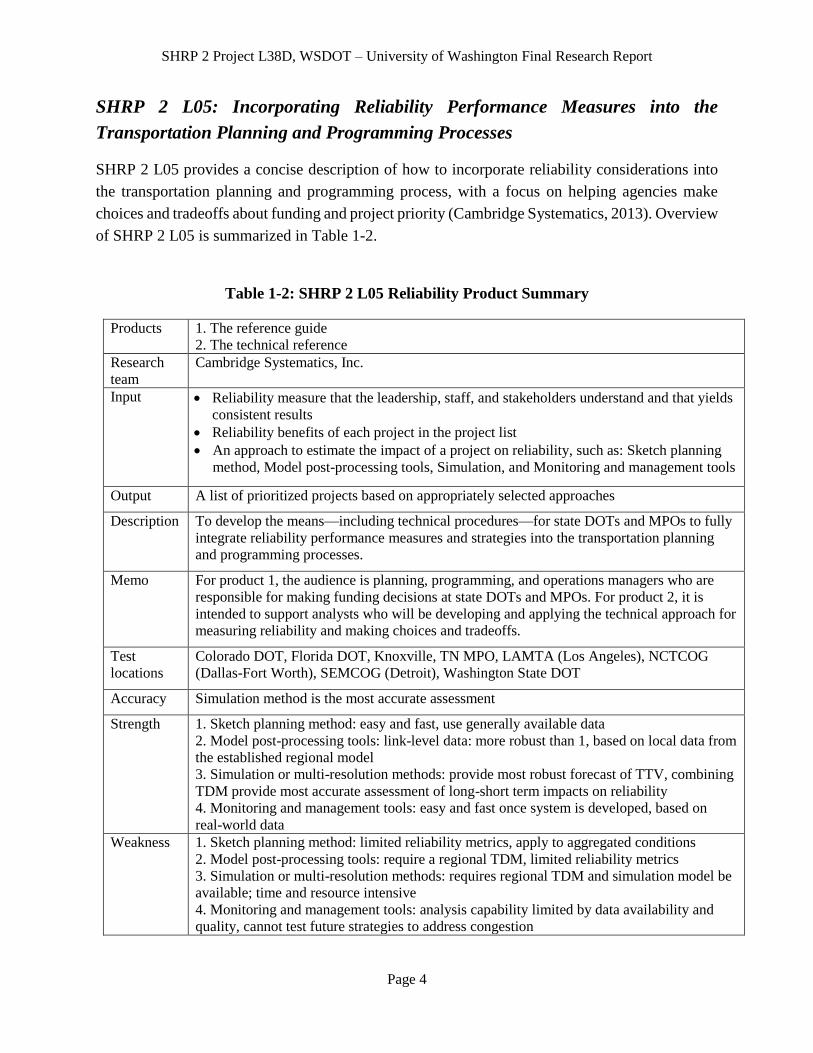
SHRP 2 L05 provides a concise description of how to incorporate reliability considerations into
the transportation planning and programming process, with a focus on helping agencies make
choices and tradeoffs about funding and project priority (Cambridge Systematics, 2013). Overview
of SHRP 2 L05 is summarized in Table 1-2.
Table 1-2: SHRP 2 L05 Reliability Product Summary
Products 1. The reference guide
2. The technical reference
Research
team
Cambridge Systematics, Inc.
Input Reliability measure that the leadership, staff, and stakeholders understand and that yields
consistent results
Reliability benefits of each project in the project list
An approach to estimate the impact of a project on reliability, such as: Sketch planning
method, Model post-processing tools, Simulation, and Monitoring and management tools
Output A list of prioritized projects based on appropriately selected approaches
Description To develop the means—including technical procedures—for state DOTs and MPOs to fully
integrate reliability performance measures and strategies into the transportation planning
and programming processes.
Memo For product 1, the audience is planning, programming, and operations managers who are
responsible for making funding decisions at state DOTs and MPOs. For product 2, it is
intended to support analysts who will be developing and applying the technical approach for
measuring reliability and making choices and tradeoffs.
Test
locations
Colorado DOT, Florida DOT, Knoxville, TN MPO, LAMTA (Los Angeles), NCTCOG
(Dallas-Fort Worth), SEMCOG (Detroit), Washington State DOT
Accuracy Simulation method is the most accurate assessment
Strength 1. Sketch planning method: easy and fast, use generally available data
2. Model post-processing tools: link-level data: more robust than 1, based on local data from
the established regional model
3. Simulation or multi-resolution methods: provide most robust forecast of TTV, combining
TDM provide most accurate assessment of long-short term impacts on reliability
4. Monitoring and management tools: easy and fast once system is developed, based on
real-world data
Weakness 1. Sketch planning method: limited reliability metrics, apply to aggregated conditions
2. Model post-processing tools: require a regional TDM, limited reliability metrics
3. Simulation or multi-resolution methods: requires regional TDM and simulation model be
available; time and resource intensive
4. Monitoring and management tools: analysis capability limited by data availability and
quality, cannot test future strategies to address congestion

SHRP 2 Project L38D, WSDOT – University of Washington Final Research Report
Page 5
SHRP 2 L07: Evaluation of the Costs and Effectiveness of Highway Design
Features to Improve Travel Time Reliability
The objective of SHRP 2 L07 is to evaluate the cost-effectiveness of geometric design treatments,
such as alternating shoulders, emergency pull-offs, etc., in reducing non-recurrent congestion
(Potts et al., 2013). Products of SHRP 2 L07 are summarized in Table 1-3.

SHRP 2 Project L38D, WSDOT – University of Washington Final Research Report
Page 6
Table 1-3: SHRP 2 L07 Reliability Product Summary
Products Spreadsheet-based analysis tool
Research
team
Midwest Research Institute (MRI)
Input 1.Treatments
2. Data:
1). Geometric data:
Number of lanes /– Lane width
Right/ Left shoulder width
Number of interchanges per mile
2). Traffic data:
Free-flow speed
Demand volume (by hour of day)
Peak hour factor (by hour of day)
Percent of trucks (by hour of day) and Percent of RVs (by hour of day)
3). Crash statistics for roadway segment:
Total annual property damage only (PDO) crashes
Total annual minor-injury crashes
Total annual serious-and fatal-injury crashes
4). Information about typical crash duration (time until cleared) :
Average crash duration (min) for PDO crashes
Average crash duration (min) for minor-injury crashes
Average crash duration (min) for serious- and fatal-injury crashes
5). Other:
Information about special events (e.g., number, percent increase in volume)
Information about work zones
3. Benefits and Costs
Output Evaluation results of cost-effectiveness for a treatment, such as travel time index (TTI),
reliability Measures of Effectiveness (MOEs).
Description What does the tool do?
Implements Project L03 models
Computes cumulative travel time index curve for untreated and treated conditions
Estimates traffic operational effectiveness of design treatments at specific locations
Compares economic benefits of various design treatments at specific locations
Memo In addition to the defined treatments available for analysis in the tool, users are also able to
evaluate any other treatment they wish, provided treatment’s effect on the three model
variables can be ascertained.
Test
locations
Seattle, WA
Accuracy The tool tends to underestimate the vehicle travel time when traffic flow is high.
Strength The tool can be used to measure the operational effectiveness as well as the economic
benefit of design treatments for a freeway segment of interest. The tool allows highway
agencies to compare the benefits and costs of implementing various nonrecurrent congestion
treatments at specific locations.
Weakness The tool interface is not very user friendly. It runs into crash sometimes
Detailed output information is not applicable, which limit the tool usability

SHRP 2 Project L38D, WSDOT – University of Washington Final Research Report
Page 7
SHRP 2 L08: Incorporation of the Non-Recurrent Congestion Factors into the
Highway Capacity Manual Methods
SHRP 2 L08 develops methods and guidance on incorporating travel time reliability into Highway
Capacity Manual (HCM) analyses. The main product of L08 is a guide that 1) describes travel time
reliability concepts for the HCM audiences, 2) provides step-by-step processes for predicting travel
time reliability for freeway and urban street facilities, and 3) illustrates sample applications of the
procedures (Kittelson and Associates, Inc., 2013). The summary of SHRP 2 L08 products is
presented in Table 1-4.

SHRP 2 Project L38D, WSDOT – University of Washington Final Research Report
Page 8
Table 1-4: SHRP 2 L08 Reliability Products Summary
Products 1. Guide describing travel time reliability concepts for HCM audience, provides step-by-step
processes for predicting travel time reliability for freeway and urban street facilities, and
illustrates example applications of the procedures.
2. FREEVAL and STREETVAL Computational Engine
Research
team
Kittelson & Associates, ITRE, Cambridge Systematics
Input Main source of travel time variability, given scenario (time of day, road condition, severity,
etc.), demand, capacity
Output HCM performance measure, the impacts of variability on performance over a year
Description determining how data and information on the impacts of differing causes of nonrecurrent
congestion (incidents, weather, work zones, special events, etc.) in the context of highway
capacity can be incorporated into the performance measure estimation procedures contained
in the HCM
Memo The methodologies contained in the HCM for predicting delay, speed, queuing, and other
performance measures for alternative highway designs are not currently sensitive to traffic
management techniques and other operation/design measures for reducing non-recurrent
congestion. A further objective is to develop methodologies to predict travel time reliability
on selected types of facilities and within corridors
Test
locations
Three locations were selected for testing in the Puget Sound Region: I-5, I-405, and SR 522
Accuracy STREETVAL: Large discrepancy between software output and ground truth data
FREEVAL: Software provides a reasonable estimation of the travel time reliability
Strength STREETVAL: Employs a powerful random scenario generation process which is a
powerful method for accounting for all possible likely scenarios
FREEVAL: Tool is able to provide a reasonable estimate of the travel time reliability. This
suggests that the principal factors affecting reliability have been accounted for.
Weakness FREEVAL: weather event with marginal impact are excluded; assume incident occurrence
and traffic demand are independent of weather condition;
STREETVAL: the methodology does not address the events: e.g. signal malfunction,
railroad crossing, signal plan transition, and fog dust storms, smoke, high winds or sun
glare.
Overall: The power in a prediction model lies in the idea that with limited information, an
outcome can be deduced. A major drawback of these tools is that they require a large
quantity of input data before they are able to make their predictions (this is especially true
of STREETVAL) and this makes these tools both difficult and costly to implement from a
practitioner’s point of view. It begs the question of whether these tools be simplified,
lessening the amount of input data requirements, and still give reasonable reliability
estimates?

SHRP 2 Project L38D, WSDOT – University of Washington Final Research Report
Page 9
SHRP 2 C11: Development of Improved Economic Analysis Tools Based on
Recommendations from SHRP 2 L03
SHRP 2 C11 provides a sketch-level planning tool based on SHRP 2 L03 research that estimates
the benefits of improving travel time reliability for use in benefit/cost analysis (Economic
Development Research Group, 2013). The SHRP 2 C11 products are summarized in Table 1-5.

SHRP 2 Project L38D, WSDOT – University of Washington Final Research Report
Page 10
Table 1-5: SHRP 2 C11 Reliability Product Summary
Products 1. Analytical tools
2. User Guide
Research
team
Economic Development Research Group, Cambridge Systematics
Input 1. Travel time reliability
Scenario data and Traffic data
Time/travel cost and reliability ratio
2. Market access
Facility type, such as marine, freight rail, air passenger, air cargo, passenger rail, etc.
Roadway improvements
3. Intermodal connectivity
Impedance decay factor and impedance data
Productivity elasticity
Impact zones and activity data
Output 1. Travel time reliability (result for base year and forecast year)
Congestion Metrics
Total annual weekday delay (veh-hrs)
Total annual weekday congestion cost for passenger and commercial vehicles,
respectively
2. Market access (result for project/policy baseline and alternative )
Accessible employment
Concentration index
Commuter costs
Effective density/potential access ‘scores’
3. Intermodal connectivity
Facility connectivity raw value
Value of time savings for facility
Weighted connectivity
4. Final result
Value of traditionally measured benefits and wider economic benefits in target year for
passenger trips and commercial (Freight delivery) trips, respectively.
Description Development of improved economic analysis tools based on recommendations from Project
C03.
Memo T-PICS is a web-based sketch planning tool that allows state departments of transportation
(DOTs), metropolitan planning organizations (MPOs), and other agencies involved in
highway capacity planning to quickly estimate the likely range of impacts of proposed
projects.
Test
locations
Uses the L03 Data Poor models as the basis
Accuracy As a sketch planning tool, it provides good enough accuracy
Strength With minimal data input, the tool adds value by incorporating change in travel time
reliability into project economic analyses
Weakness The calculation methodology is designed to capture the benefits of major capacity projects.
It is not sensitive to the travel time reliability changes associated with improvements at
roadway intersections, interchanges and freeway ramps.

SHRP 2 Project L38D, WSDOT – University of Washington Final Research Report
Page 11
1.3 Research Objectives
This research project has two major objectives:
To provide feedback to SHRP 2 on the applicability and usefulness of the products tested;
and
To assist agencies in moving reliability into their business practices through testing of the
products developed by the five SHRP 2 Reliability projects.
For testing the SHRP 2 Reliability Data and Analytical Products, the research procedure consists
of three major steps: a) data compilation, integration and quality control; b) experiment design for
testing different products; and c) test results evaluation and possible improvements. The L38D
research team has followed the proposed procedure through the pilot testing of all the committed
research products.
1.4 Final Report Organization
This report comprises of nine chapters. Chapter 1 introduces the general background for the SHRP
2 L38 project and hence summaries the objectives of the research project. The general testing
approach is presented in Chapter 2. Chapter 3 describes the data compilation and quality control
process applied to the data used for this study. Chapters 4-8 provide the details of the research in
analyzing reliability and improvement strategies, including site selection, case description, testing
results, comparisons, and discussions of the L38 tools. Based on the testing results, Chapter 9
concludes the research and offers potential improvement directions for the tested SHRP 2
Reliability products.

SHRP 2 Project L38D, WSDOT – University of Washington Final Research Report
Page 12
CHAPTER 2 RESEARCH APPROACH
Given the complexity in each transportation project’s design, construction, evaluation, and
decision making and the small sample possible to use for testing the selected products, the research
team made effort to ensure the reliability of the test results in two aspects: (1) setting up a dedicated
steering committee to provide guidance and advice to the research team and (2) developing a
thorough testing procedure for different types of products.
2.1 Steering Committee
A steering committee for the SHRP 2 L38D research project was formed upon the start of this
research project. The committee members include Daniela Bremmer, Director of WSDOT’s
Strategic Assessment Office and chair of the TRB Committee on Performance Measurement,
Patrick Morin, Operations Manager of the WSDOT Capital Program Development and
Management Office, Bill Legg, Washington State Intelligent Transportation System Operations
Engineer, Shuming Yan, Deputy Director of the WSDOT Urban Planning Office, etc. They are
from all relevant fields including transportation planning, traffic operations, urban corridor
management, performance measurement and economic impacts, and project prioritization, and are
very familiar with the past and ongoing projects suitable for this study.
Principal Investigator (PI) and the Washington State Traffic Engineer, John Nisbet, calls regular
meetings of the research team to check progress and collaborates research efforts between the UW
and WSDOT. He also organizes quarterly steering committee meetings to review research
activities, suggest new research actions, and coordinate research efforts.
2.2 Test Procedure
A systematic procedure for testing the SHRP 2 Reliability products was developed based on
foreseeable needs in WSDOT’s practice. Please see Figure 2-1 for details. Our test procedure
covers both types of products: (1) models or procedures and (2) software tools. As shown in Figure
2-1, the test processes of the two types of products interact with each other because the computer
software tools are typically the implementations of the methods or procedures.
2.2.1 Methods or Procedure Testing
Models or procedures are typically developed based on assumptions. The reasonableness of these
assumptions are critical to the applicability of the methods. Specific mathematical equations
employed are also important and a tradeoff between complexity and applicability must be made
carefully in developing a model or procedure. Thus the accuracy of the model or procedure needs

SHRP 2 Project L38D, WSDOT – University of Washington Final Research Report
Page 13
to be evaluated. Considering that the data used in calibrating the model may not be representative
to all locations and time periods, both temporal and spatial transferability must be tested.
Excel Based Tool Test(Application Test)Technical Model or Procedure Test
Experimental Design
Test Site Selection
Data Compilation
Test Objectives
Data & Analysis Meth
Data Compilation
Testbed Installation
Data Quality Control
Testing
Assumptions
Spatial Transferability
Temporal
Transferability
Test-bed DesignCompare
Interface
User-friendly
Necessary
Guidance
Help Documents
Default Setup
Layout
Installation
SuccessfulValidation
Algorithm
Theory
Calculation
Scalability
Various Scales
Analysis and Feedback
Result Analysis Conclusions Feedback/Potential Refinements
Figure 2-1 General Approach for Pilot Testing of the SHRP 2 L38 Products
Following such a logic, the research team developed a three step procedure for testing model or
procedure type of products:
1. Experiment Design.
(1) Test objectives. This step is driven by the test objectives or the key questions to answer by the
experiment. Test objectives must be clearly set as the first step of the experiment design. In
designing the test details, the following factors are important to consider:
(2) Test site selection. Random sampling from those qualified project sites is important in avoiding
bias. It also allows uses of general probability theory in data analysis. Test sites should offer

SHRP 2 Project L38D, WSDOT – University of Washington Final Research Report
Page 14
observations for comparative analysis. The SHRP 2 Reliability models or procedure products may
include numerous control variables. To evaluate the impact of a particular variable, the conditions
with and without the variable needs to be observed. Also, a specific condition is better replicable
to reduce the effect of uncontrolled variation and quantify uncertainty when needed.
(3) Test-bed configuration design. Depending on the kinds of data needed and whether or not they
are observable, further instrumentation of sensors for the desired types of data may be needed.
(4) Data collection and proposed analytical approach. Data collection location and time period
need to be determined to support the planned tests. Given the nature of the model or procedure
products to be tested in this research, simple validation of the model predicted results using field
data and before-and-after analysis of specific highway treatments are sufficient in this study.
2. Data Compilation
This step focuses on all the technical details in collecting and storing data, and make the data sets
ready to use. A wide range of urban freeway and arterial data are compiled. The data collected for
this study include 1) traditional static sensor data (loop, camera, etc.); 2) roadway geometric profile
data; 3) incident and crash data (Washington Incident Tracking System data); 4) weather data; and
5) traffic operation and management data (such as Active Traffic Management (ATM) control
data).
Data quality control is an important component as low quality data will interfere the test procedure
and may mislead the research. Data quality control procedures developed by WSDOT and the
University of Washington are used to enhance data quality for the pilot testing. Data fusion and
mining are performed to integrate traffic data with weather and incident data on a regional map
basis to investigate travel time reliability under recurring and non-recurring congestion conditions.
More details of the data collection and quality control procedure are described in Chapter 3.
3. Testing
In this testing step, accuracy and transferability, including both temporal and spatial transferability,
of the model or procedure products will be evaluated using the data collected from our study sites.
2.2.2 Computer Tool Testing
All the computer tool products were Microsoft Excel-based applications. The key of the tests of
such products is whether an application meets the requirements that guided its design and
implementation. Specifically, the requirements may include operability, usability, performance,
and scalability.
SHRP 2 Project L38D, WSDOT – University of Washington Final Research Report
Page 15
Operability test includes compatibility test of the commonly used operating systems. If the
software application cannot be installed or operated in a specific operating system or Excel version,
then it fails the operability test.
Usability test evaluates if the software is easy to understand and use. User interface is important
for user-computer interactions and thus plays an important role in usability. Evaluation of usability
is based on the following factors: (1) user interface’s level friendliness, (2) sufficient guidance and
help information accessible when using the software, (3) default configurations and explanation
of the input parameters needed to start the software, and (4) layout of the modules and data output.
Performance test focuses on correctness and efficiency. If a software application does not
implement the correct logic or method, then it fails the performance test. Even if the method or
procedure is correctly implemented, an application may still fails its performance test if the
efficiency is beyond tolerable range.
Scalability test for this research project refers to whether the software tool can be applied to a much
smaller or much bigger project than the ones used to develop them. Scalability is important for
future applications to transportation projects with varying scales.
2.2.3 Result Analysis and Feedback
A set of measures of effectiveness (MOEs) is carefully selected for each test. The computed MOEs
will be compared with those used by WSDOT in practice. Over the past decades, WSDOT has
completed a number of projects that are appropriate for testing and before-and-after analysis on
travel time reliability. Specifically, the following projects are chosen as study projects for SHRP
2 L38:
Corridors used for the WSDOT Gray Notebook production are used to test SHRP 2 L02
products. WSDOT has been monitoring corridor travel time for the quarterly Gray
Notebook performance evaluation report since 2001. The Gray Notebook provides updates
on system performance and project delivery on the corridor and statewide levels.
Additionally, the Gray Notebook is used for testing and evaluating products of SHRP 2
L02.
Among the Moving Washington projects, corridors along I-5 and I-405, and State Route
522 are used for testing the methods and analytical tools from SHRP 2 L08.
I-5 JBLM is chosen as a case study for testing the effectiveness and usability of the products
from SHRP 2 L05 and C11. To test the five-step procedure from SHRP 2 L05, a couple of
projects in this region have been prioritized within the 10-year investment strategy. By
applying the SHRP 2 C11 tool on I-5 JBLM projects, both traditionally measured benefits
and wider economic benefits over the past years can be analyzed, and the tool’s usability
and effectiveness can be tested.

SHRP 2 Project L38D, WSDOT – University of Washington Final Research Report
Page 16
At the end of each test, problems identified through the test and recommended improvements are
made to help the SHRP 2 Reliability program make these tool more useful in future practice.

SHRP 2 Project L38D, WSDOT – University of Washington Final Research Report
Page 17
CHAPTER 3 DATA COMPILATION AND INTEGRATION
3.1 Test Site Selection
Table 3-1 shows all the reliability products selected to test and their test objectives. Following the
needs of testing all the products, the SHRP 2 L38D research team and its steering committee met
and generated a list of candidate test sites. Among those qualified candidate sites, a number of test
sites are selected and considered representative to normal roadway conditions in Washington. A
brief description of each site is given below:
Test Site A: I-5 between the interchanges with I-405. This facility operates in over saturated
conditions during both morning and afternoon peak periods near downtown Seattle. Loop detectors
are deployed every half a mile on the main stream lanes and on the on and off ramps. This test site
is used for testing products of L02, L07, and L08.
Test Site B: I-405 between the interchanges with I-5. This facility also operates in over saturated
conditions during both morning and afternoon peak periods near downtown Bellevue. Loop
detectors are deployed every half a mile on the main stream lanes and on the on and off ramps.
This test site is used for testing products of L02 and L08.
Table 3-1 The Reliability Products Selected to Test and the Test Objectives
Products Description Test objectives
L02 Establishing monitoring programs for travel time
reliability.
Effectiveness
L05 The guide for state DOTs and MPOs to fully
integrate reliability performance measures and
strategies into the transportation planning and
programming processes.
Usability, Performance
L07 Evaluation of the cost-effectiveness of geometric
design treatments, such as alternating shoulders,
emergency pull-offs, etc., in reducing non-recurrent
congestion.
Operability, Usability,
Performance
L08 Guidance on incorporating travel time reliability
into Highway Capacity Manual (HCM) analyses.
Operability, Usability,
Performance
C11 Development of improved economic analysis tools
based on recommendations from Project C03.
Usability, Performance
SHRP 2 Project L38D, WSDOT – University of Washington Final Research Report
Page 18
Test Site C: I-5 Joint Base Lewis-McChord (JBLM). As the single largest employer in Pierce
County and the third largest in Washington State, JBLM plays an important role in our
communities. I-5 JBLM is the major thoroughfare for freight and commuter traffic in this region.
In recent years, significant increases in traffic congestion have been witnessed due to the regional
growth, with longer commute times, longer duration of congestion, impacts to freight movement,
military operations, and the overall economy. This test site is used for testing products of L05 and
C11.
Test Site D: SR-522 between the intersections with 68th AVE NE and 83rd PL NE. This is a busy
signalized corridor serving as an alternative of I-90 and SR-520 for traffic crossing Lake
Washington. It also connects I-5 and I-405. It gets congested during the peak hours and carries
relatively low demand during night time. This test site is used for testing products of L08.
3.2 Dataset Creation
Based on the selected test sites and the needs of data for the tests, the L38D research team reviewed
available traffic data in each site and developed further data collection plans to ensure the coverage
and quality of data. In general, our study data are collected from two types of facilities: urban
freeways and signalized arterials.
Urban Freeway Data – WSDOT maintains a loop detector station approximately every half a
mile in the central Puget Sound area freeways. Urban freeway traffic volume and occupancy data
are obtained from the WSDOT loop detector network via the STAR Lab fiber connections to the
WSDOT Northwest Region’s traffic system management center (TSMC), where loop data are
stored and disseminated. In addition to the loop detector data, INRIX probe vehicle speed data,
traffic incident data, weather data, and roadway geometric data are also archived and used for
urban freeway analysis.
Signalized Arterial Data – Signalized arterial traffic data are acquired from two sources: in-road
loop detectors and Automatic License Plate Readers (ALPRs). Loop detectors provide volume and
occupancy data. ALPRs offer travel time measurements. Besides these two data sets, weather and
roadway geometric data are also obtained and used in the analysis of signalized arterials. However,
these existing data sets are not sufficient for arterial analysis. Video-based onsite data collection
was conducted to obtain directional vehicle movements at signalized intersections on this corridor.
Specifically, the following data sets are created for this research project:

SHRP 2 Project L38D, WSDOT – University of Washington Final Research Report
Page 19
Dataset A: Loop Detector Data
Dataset A consists of direct loop detector measurements (volume and occupancy for single loops
and traffic speed and bin volumes for dual loops) and delay estimates based on loop detector data
for Test Sites A (I-5), B (I-405), and D (SR-522). Dataset creation involves obtaining, cleaning,
and integrating data collected by the research team. There are several challenges within this
process. Among them are processing, reviewing, and reducing raw data into summaries suitable
for analysis and conflating traffic data with geospatial data.
Inductive loop detectors are widely deployed in Washington State for the purpose of monitoring
traffic conditions and freeway performance. WSDOT maintains and manages loop detectors on
Washington state highways as well as those on Interstate freeways within Washington State. For
the purpose of traffic management, the State of Washington is divided into six regions: Northwest,
North Central, Eastern, South Central, Southwest, and Olympic. Relevant to this project, there are
approximately 4200 single or dual loop detectors installed in the Northwest Region, which are
used to monitor traffic condition around the Seattle metropolitan area.
There are two general types of loop detectors in Washington State, single loop and dual loop.
Single loop detectors are only capable of detecting whether a vehicle is present or absent, which
allows volume and occupancy to be measured directly. Dual loop detectors, on the other hand, are
composed of two single loop detectors placed a short distance apart, thereby allowing travel speed
to be estimated from the difference in arrival time between upstream and downstream detectors.
Vehicle length can also be estimated from dual loop detector data, based on the estimated speed
and measured detector occupancy.
Loop detector data in Washington State is available at both 20-second and 5-minute aggregation
intervals. Note that all data is collected at the 20-second aggregation level, and is further
aggregated into 5-minute periods. The key information for the 20-second and 5-minute aggregation
intervals is listed in Table 3-2 and Table 3-3, respectively. WSDOT primarily uses the 5-minute
aggregation level loop data for freeway performance monitoring and reporting (Wang et al., 2008).
The “LoopID” field in Table 3-2 and Table 3-3 is a unique identifier for each loop detector which
can be matched to a detector cabinet, and multiple loop detectors can be connected to a given
cabinet. A Cabinets table contains descriptive and location information for each cabinet, and so
associating loops with the cabinets they are connected to facilitates locating the loops using cabinet
milepost and route. The key information contained in the cabinets table is listed in Table 3-4.
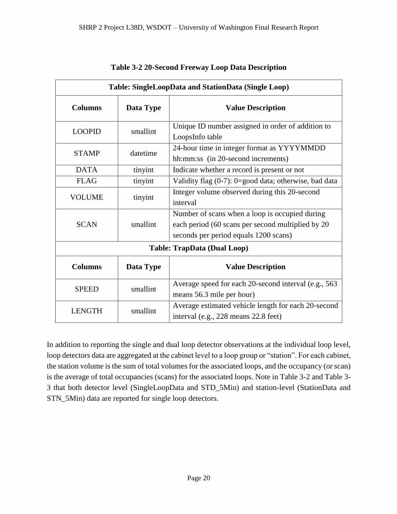
SHRP 2 Project L38D, WSDOT – University of Washington Final Research Report
Page 20
Table 3-2 20-Second Freeway Loop Data Description
Table: SingleLoopData and StationData (Single Loop)
Columns Data Type Value Description
LOOPID smallint Unique ID number assigned in order of addition to
LoopsInfo table
STAMP datetime 24-hour time in integer format as YYYYMMDD
hh:mm:ss (in 20-second increments)
DATA tinyint Indicate whether a record is present or not
FLAG tinyint Validity flag (0-7): 0=good data; otherwise, bad data
VOLUME tinyint Integer volume observed during this 20-second
interval
SCAN smallint
Number of scans when a loop is occupied during
each period (60 scans per second multiplied by 20
seconds per period equals 1200 scans)
Table: TrapData (Dual Loop)
Columns Data Type Value Description
SPEED smallint Average speed for each 20-second interval (e.g., 563
means 56.3 mile per hour)
LENGTH smallint Average estimated vehicle length for each 20-second
interval (e.g., 228 means 22.8 feet)
In addition to reporting the single and dual loop detector observations at the individual loop level,
loop detectors data are aggregated at the cabinet level to a loop group or “station”. For each cabinet,
the station volume is the sum of total volumes for the associated loops, and the occupancy (or scan)
is the average of total occupancies (scans) for the associated loops. Note in Table 3-2 and Table 3-
3 that both detector level (SingleLoopData and STD_5Min) and station-level (StationData and
STN_5Min) data are reported for single loop detectors.

SHRP 2 Project L38D, WSDOT – University of Washington Final Research Report
Page 21
Table 3-3 5-Minute Freeway Loop Data Description
Table: STD_5Min and STN_5Min (Single Loop)
Columns Data
Type Value Description
LOOPID smallint Unique ID number assigned in order of addition to
LoopsInfo table
STAMP datetime 24-hour time in integer format as YYYYMMDD
hh:mm:ss (increased by 5 minutes)
FLAG tinyint Good/bad data flag with 1 = good and 0 = bad (simple
diagnostics supplied by WSDOT)
VOLUME tinyint Integer volume observed during each 5-minute interval
OCCUPANCY smallint Percentage of occupancy expressed in tenths to obtain
integer values (6.5% = 65)
PERIODS smallint
The number of 20-second readings incorporated into
this 5-minute record (15 is ideal, less than 15 almost
always indicates that volume data are unusable unless
adjusted to account for missing intervals).
Table: TRAP_5Min (Dual Loop)
Columns Data
Type Value Description
SPEED smallint Average speed for each 5-minute interval (e.g., 563
means 56.3 mile per hour)
LENGTH smallint Average estimated vehicle length for each 5-minute
interval (e.g., 228 means 22.8 feet)
WSDOT makes both 20-second and 5-minute loop detector data available for download using an
online FTP website. Detector data are periodically retrieved from the posted FTP website,
formatted, and stored in the STAR Lab Microsoft SQL Server databases using an automated
computer program written in Microsoft Visual C#. For the pilot testing of SHRP 2 L02, L07, L08
and C11 products, traffic volume data along the Test Sites A, B, and D corridors were collected.
Figure 3-1 illustrates most of the loop locations along I-5 and I-405 in the northwest region of
Washington State. 5-min traffic volume data was collected for the time period from January 2009
to June 2013. Figure 3-2 illustrates the traffic flow map based on the 5-min loop data collected at
5:30 p.m. December 11, 2012. Loop detectors along SR-522 are shown together with the other
available sensors in Figure 3-3.
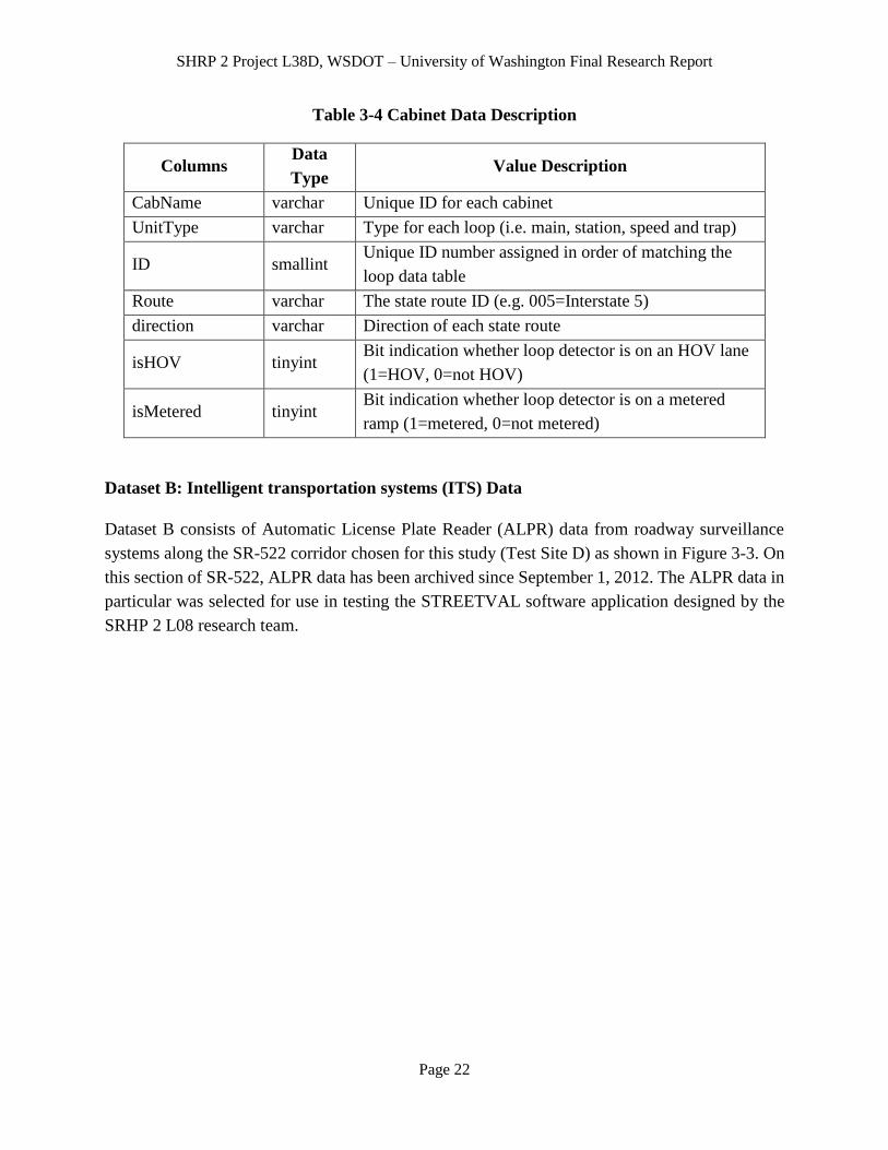
SHRP 2 Project L38D, WSDOT – University of Washington Final Research Report
Page 22
Table 3-4 Cabinet Data Description
Columns Data
Type Value Description
CabName varchar Unique ID for each cabinet
UnitType varchar Type for each loop (i.e. main, station, speed and trap)
ID smallint Unique ID number assigned in order of matching the
loop data table
Route varchar The state route ID (e.g. 005=Interstate 5)
direction varchar Direction of each state route
isHOV tinyint Bit indication whether loop detector is on an HOV lane
(1=HOV, 0=not HOV)
isMetered tinyint Bit indication whether loop detector is on a metered
ramp (1=metered, 0=not metered)
Dataset B: Intelligent transportation systems (ITS) Data
Dataset B consists of Automatic License Plate Reader (ALPR) data from roadway surveillance
systems along the SR-522 corridor chosen for this study (Test Site D) as shown in Figure 3-3. On
this section of SR-522, ALPR data has been archived since September 1, 2012. The ALPR data in
particular was selected for use in testing the STREETVAL software application designed by the
SRHP 2 L08 research team.
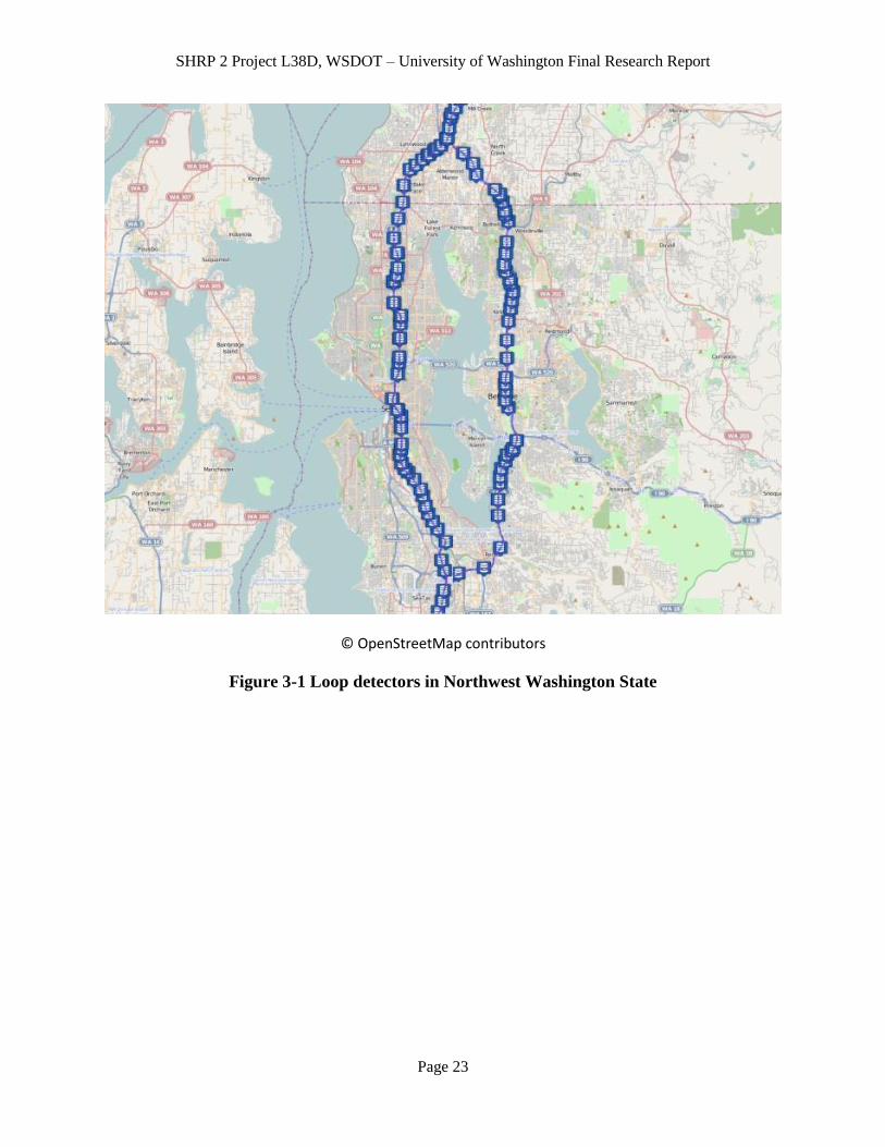
SHRP 2 Project L38D, WSDOT – University of Washington Final Research Report
Page 23
© OpenStreetMap contributors
Figure 3-1 Loop detectors in Northwest Washington State
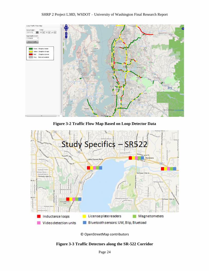
SHRP 2 Project L38D, WSDOT – University of Washington Final Research Report
Page 24
Figure 3-2 Traffic Flow Map Based on Loop Detector Data
© OpenStreetMap contributors
Figure 3-3 Traffic Detectors along the SR-522 Corridor
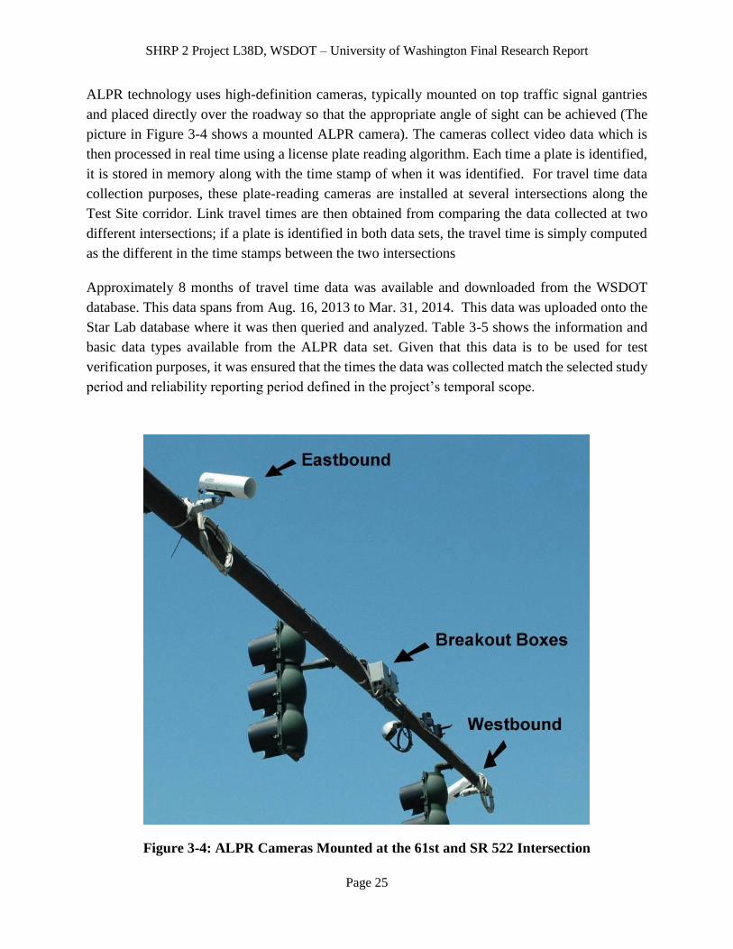
SHRP 2 Project L38D, WSDOT – University of Washington Final Research Report
Page 25
ALPR technology uses high-definition cameras, typically mounted on top traffic signal gantries
and placed directly over the roadway so that the appropriate angle of sight can be achieved (The
picture in Figure 3-4 shows a mounted ALPR camera). The cameras collect video data which is
then processed in real time using a license plate reading algorithm. Each time a plate is identified,
it is stored in memory along with the time stamp of when it was identified. For travel time data
collection purposes, these plate-reading cameras are installed at several intersections along the
Test Site corridor. Link travel times are then obtained from comparing the data collected at two
different intersections; if a plate is identified in both data sets, the travel time is simply computed
as the different in the time stamps between the two intersections
Approximately 8 months of travel time data was available and downloaded from the WSDOT
database. This data spans from Aug. 16, 2013 to Mar. 31, 2014. This data was uploaded onto the
Star Lab database where it was then queried and analyzed. Table 3-5 shows the information and
basic data types available from the ALPR data set. Given that this data is to be used for test
verification purposes, it was ensured that the times the data was collected match the selected study
period and reliability reporting period defined in the project’s temporal scope.
Figure 3-4: ALPR Cameras Mounted at the 61st and SR 522 Intersection
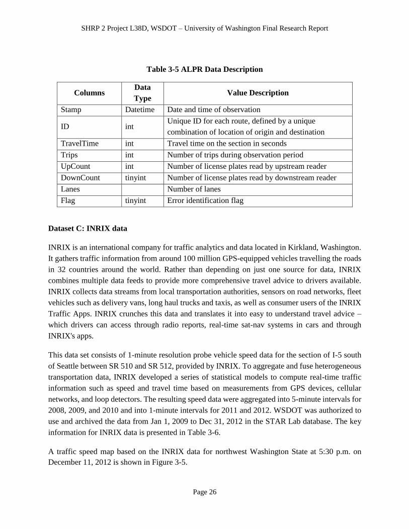
SHRP 2 Project L38D, WSDOT – University of Washington Final Research Report
Page 26
Table 3-5 ALPR Data Description
Columns Data
Type Value Description
Stamp Datetime Date and time of observation
ID int Unique ID for each route, defined by a unique
combination of location of origin and destination
TravelTime int Travel time on the section in seconds
Trips int Number of trips during observation period
UpCount int Number of license plates read by upstream reader
DownCount tinyint Number of license plates read by downstream reader
Lanes Number of lanes
Flag tinyint Error identification flag
Dataset C: INRIX data
INRIX is an international company for traffic analytics and data located in Kirkland, Washington.
It gathers traffic information from around 100 million GPS-equipped vehicles travelling the roads
in 32 countries around the world. Rather than depending on just one source for data, INRIX
combines multiple data feeds to provide more comprehensive travel advice to drivers available.
INRIX collects data streams from local transportation authorities, sensors on road networks, fleet
vehicles such as delivery vans, long haul trucks and taxis, as well as consumer users of the INRIX
Traffic Apps. INRIX crunches this data and translates it into easy to understand travel advice –
which drivers can access through radio reports, real-time sat-nav systems in cars and through
INRIX's apps.
This data set consists of 1-minute resolution probe vehicle speed data for the section of I-5 south
of Seattle between SR 510 and SR 512, provided by INRIX. To aggregate and fuse heterogeneous
transportation data, INRIX developed a series of statistical models to compute real-time traffic
information such as speed and travel time based on measurements from GPS devices, cellular
networks, and loop detectors. The resulting speed data were aggregated into 5-minute intervals for
2008, 2009, and 2010 and into 1-minute intervals for 2011 and 2012. WSDOT was authorized to
use and archived the data from Jan 1, 2009 to Dec 31, 2012 in the STAR Lab database. The key
information for INRIX data is presented in Table 3-6.
A traffic speed map based on the INRIX data for northwest Washington State at 5:30 p.m. on
December 11, 2012 is shown in Figure 3-5.
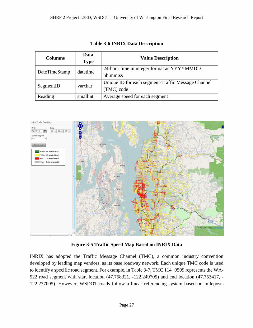
SHRP 2 Project L38D, WSDOT – University of Washington Final Research Report
Page 27
Table 3-6 INRIX Data Description
Columns Data
Type Value Description
DateTimeStamp datetime 24-hour time in integer format as YYYYMMDD
hh:mm:ss
SegmentID varchar Unique ID for each segment-Traffic Message Channel
(TMC) code
Reading smallint Average speed for each segment
Figure 3-5 Traffic Speed Map Based on INRIX Data
INRIX has adopted the Traffic Message Channel (TMC), a common industry convention
developed by leading map vendors, as its base roadway network. Each unique TMC code is used
to identify a specific road segment. For example, in Table 3-7, TMC 114+0509 represents the WA-
522 road segment with start location (47.758321, -122.249705) and end location (47.753417, -
122.277005). However, WSDOT roads follow a linear referencing system based on mileposts
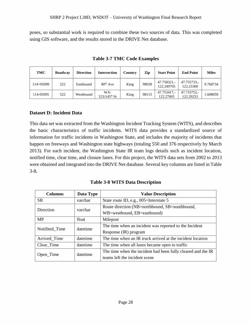
SHRP 2 Project L38D, WSDOT – University of Washington Final Research Report
Page 28
poses, so substantial work is required to combine these two sources of data. This was completed
using GIS software, and the results stored in the DRIVE Net database.
Table 3-7 TMC Code Examples
TMC Roadway Direction Intersection Country Zip Start Point End Point Miles
114+05099 522 Eastbound 80th Ave King 98028 47.758321,-
122.249705
47.755733,-
122.23368 0.768734
114-05095 522 Westbound WA-
523/145th St King 98115
47.753417,-
122.27005
47.733752,-
122.29253 1.608059
Dataset D: Incident Data
This data set was extracted from the Washington Incident Tracking System (WITS), and describes
the basic characteristics of traffic incidents. WITS data provides a standardized source of
information for traffic incidents in Washington State, and includes the majority of incidents that
happen on freeways and Washington state highways (totaling 550 and 376 respectively by March
2013). For each incident, the Washington State IR team logs details such as incident location,
notified time, clear time, and closure lanes. For this project, the WITS data sets from 2002 to 2013
were obtained and integrated into the DRIVE Net database. Several key columns are listed in Table
3-8.
Table 3-8 WITS Data Description
Columns Data Type Value Description
SR varchar State route ID, e.g., 005=Interstate 5
Direction varchar Route direction (NB=northbound, SB=southbound,
WB=westbound, EB=eastbound)
MP float Milepost
Notifited_Time datetime The time when an incident was reported to the Incident
Response (IR) program
Arrived_Time datetime The time when an IR truck arrived at the incident location
Clear_Time datetime The time when all lanes became open to traffic
Open_Time datetime The time when the incident had been fully cleared and the IR
teams left the incident scene

SHRP 2 Project L38D, WSDOT – University of Washington Final Research Report
Page 29
Dataset E: Weather Data
This data set consists of weather data from stations in Washington State. Weather data was sourced
from a website maintained be the University of Washington Atmospheric Sciences Department,
which provides access to hourly observations from 209 weather stations through the National
Oceanic and Atmospheric Administration (NOAA). Weather data is automatically fetched from
the website and stored in a STAR Lab database using a JAVA-based computer program written
for this purpose. Several key pieces of information are shown in Table 3-9. Weather data is
visualized geographically on the DRIVE Net system using the latitude and longitude information
associated with each weather station, and can be viewed at www.uwdrive.net.
Table 3-9 Weather Data Description
Columns Data Type Value Description
name Varchar The weather station identifier
timestamp Datetime 24 hour time in integer format as YYYYMMDD hh:mm:ss
visibility Smallint Visibility in miles
temp Smallint Temperature in degrees Fahrenheit
dewtemp Smallint Dew point temperature
wind_direction Smallint Direction wind is coming from in degrees; from the south is
180
wind_speed Smallint Wind Speed in knots
pcpd Smallint Total 6 hr precipitation at 00z, 06z, 12z and 18z; 3hr total for
other times. Amounts in hundredths of an inch.
Dataset F: Roadway Geometric Data
This data set contains roadway geometry sourced from WSDOT’s GIS and Roadway Data Office
(GRDO). The GeoData Distribution Catalog is maintained by GRDO to promote data exchange,
and can be accessed online at http://www.wsdot.wa.gov/mapsdata/geodatacatalog/. This data is
made available in the form of ESRI shape files, which is an industry standard digital format for
geospatial data. Available geometric data sets include lane count, roadway widths, ramp locations,
shoulder widths, and surface types. In order to allow geometric elements to be located using the
WSDOT linear referencing systems, State Route ID and milepost information are included in this
data set. A substantial quantity of such geometric data have been obtained and stored in a spatial
database as part of the STAR Lab DRIVE Net system, and made available for this project.

SHRP 2 Project L38D, WSDOT – University of Washington Final Research Report
Page 30
3.3 Data Quality Control
For this project, a great deal of emphasis has been placed on Data Quality Control (DQC).
Fortunately, much of the necessary data quality assurance procedure has previously been
developed and implemented in the DRIVE Net System. Most notably, a two-step data quality
control procedure for loop detector data is developed as illustrated in Figure 3-6. The raw loop
data are first subjected to a series of error detection tests to identify missing and erroneous data.
These data are flagged for further corrections and remedies. Several statistical algorithms are
developed to estimate the missing data and replace those erroneous records. The corrected data is
periodically stored in the database for use in further analysis.
The 20-second and 5-minute loop data, as well as the ALPR data are all processed for quality
control purposes.
3.3.1 Loop Detector DQC Procedure
Figure 3-6 shows how incoming loop detector data is processed in the DQC procedure. Error
detection algorithms identify and remove erroneous observations based on controller hardware
diagnostics and value thresholding, and then sensitivity issues are detected and corrected using a
Gaussian mixture model algorithm. All loop detector quality control is completed according to the
methodologies outline in (Wang et al., 2013). Raw (unadjusted) loop detector data is retained
throughout the process as back up as well as to quantify the efficacy of the quality control
algorithms. This raw data also serves as a benchmark for comparison purposes in performance
measurements and in the effectiveness of data quality control algorithms (Wang et al., 2013).
When data is retrieved from the WSDOT FTP site, basic error detection results are already present
in the form of simple hardware diagnostics error flags. This process is run at the cabinet level, and
reports the presence of common loop detector quality issues such as short pulses, loop chatter, and
values outside of allowable volume/occupancy ranges as well as whether or not the loop has been
manually deactivated. (Ishimaru and Hallenbeck, 1999). Based on these flags, a loop reporting at
least 90% “good” data is considered acceptable for use in analysis (with erroneous data removed).
A series of additional error detection procedures are performed on the data prior to uploading into
the DRIVE Net platform, primarily based on value thresholding. These procedures are outline
below, for further information see Wang et al. (2013).
Values outside the established thresholds are marked as missing, though in many cases this does
not mean the observations are the result of a hardware malfunction. For example, when no vehicles
pass over the detector in a given interval (which frequently happens during low volume time
periods), the volume, occupancy, and speed will all be reported as zero. This simply means that no
data are available for that interval, and in this case data must be marked as missing. The
thresholding criteria (based on Chen et al. (2003)) are listed below.
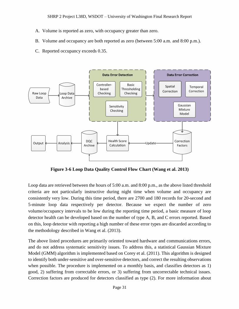
SHRP 2 Project L38D, WSDOT – University of Washington Final Research Report
Page 31
A. Volume is reported as zero, with occupancy greater than zero.
B. Volume and occupancy are both reported as zero (between 5:00 a.m. and 8:00 p.m.).
C. Reported occupancy exceeds 0.35.
Figure 3-6 Loop Data Quality Control Flow Chart (Wang et al. 2013)
Loop data are retrieved between the hours of 5:00 a.m. and 8:00 p.m., as the above listed threshold
criteria are not particularly instructive during night time when volume and occupancy are
consistently very low. During this time period, there are 2700 and 180 records for 20-second and
5-minute loop data respectively per detector. Because we expect the number of zero
volume/occupancy intervals to be low during the reporting time period, a basic measure of loop
detector health can be developed based on the number of type A, B, and C errors reported. Based
on this, loop detector with reporting a high number of these error types are discarded according to
the methodology described in Wang et al. (2013).
The above listed procedures are primarily oriented toward hardware and communications errors,
and do not address systematic sensitivity issues. To address this, a statistical Gaussian Mixture
Model (GMM) algorithm is implemented based on Corey et al. (2011). This algorithm is designed
to identify both under-sensitive and over-sensitive detectors, and correct the resulting observations
when possible. The procedure is implemented on a monthly basis, and classifies detectors as 1)
good, 2) suffering from correctable errors, or 3) suffering from uncorrectable technical issues.
Correction factors are produced for detectors classified as type (2). For more information about
Spatial
Correction

SHRP 2 Project L38D, WSDOT – University of Washington Final Research Report
Page 32
this algorithm and the specifics of implementation, see Wang et al. (2013). Based on the three
quality control procedures described above, a health score for each loop detector observation is
computed as an indicator of reliability and stored in the loop detector database.
For loop detectors reporting a sufficient number of non-missing observations, corrections are
applied to recover the records flagged by the error detection algorithm. Different corrections are
applied based on the scenario and the availability of adjacent observations, listed below:
1. Replacement by spatial interpolation
2. Replacement by temporal interpolation
3. GMM sensitivity correction
Each of these correction approaches will be discuss briefly below.
(1) Spatial Interpolation
For loop detector records flagged by the error detection algorithm or simply missing from the data
set due to hardware malfunction, records from adjacent detectors are used to replace the missing
observations when possible. There are two ways in which this is done, the selection of which
depends on the availability of nearby detector observations marked as “good”.
In scenario 1, interpolation is performed using data from lanes adjacent to that of the missing or
erroneous record. This is the preferred approach, as there is in general a high correlation between
speed, volume, and occupancy in adjacent lanes at any given location. However, this is not always
possible, because certain error types (e.g. communications failure) often impact all detectors on a
given cabinet. In this case, multiple detectors at the cabinet of interest will report missing or
erroneous records for one or more intervals.
In scenario 2, interpolation is performed using data from detectors positioned upstream and
downstream of the missing or erroneous record. This approach is applied when the method applied
in scenario 1 is impossible due to lack of adjacent lane records.
(2) Temporal Interpolation
Temporal interpolation is used to fill in missing values when only a single consecutive observation
is missing. That is, it is only applied when records are present both before and after the missing or
erroneous observation in the time series. This method is preferable to spatial interpolation, but
cannot be applied when multiple consecutive observations are marked missing. Note that, if a
detector has been marked as malfunctioning due to a high number of observations flagged as “bad”,
spatial interpolation cannot be performed.
Spatial and temporal interpolation are imputation processes for filling in missing values, where
data is not present in the data set due either to hardware malfunction or to having been removed

SHRP 2 Project L38D, WSDOT – University of Washington Final Research Report
Page 33
by the error detection algorithms. What is presented here is a very brief summary; refer to the
Wang et al. (2013) for more thorough description of the methodology and implementation.
(3) GMM Correction
The Gaussian Mixture Model (GMM) algorithm simulates the distribution of occupancy as a
mixture of Gaussian distributions. This allows the ratio of between normal and biased occupancy
to be calculated and used to correct records from over-sensitive or under-sensitive loops. As
mentioned previously, produces a flag assigned to each detector by month, designating the detector
as one of the following: 1) good, 2) suffering from correctable errors, or 3) suffering from
uncorrectable technical issues. For those detectors classified as (2), a correction factor is estimated
based on the ratio between normal and biased occupancy. The correction factor is computed based
on knowledge of vehicle length distributions, and is estimated monthly using intervals during
which only a single vehicle passed over the detector (i.e. during low volume periods). For a
thorough description of the GMM procedure, refer to Wang et al. (2013) and Corey et al. (2011).
The GMM algorithm is implemented in a software package written in SQL, JAVA, and R
programing languages. A Graphical User Interface has been developed to ease execution, shown
in Figure 3-7.
3.3.2 ITS DQC Procedure
While ALPR travel time estimates are in general reliable, some unrealistically high travel times
are recorded due to the opportunity for vehicles to make incomplete trips through a corridor.
Typically, this happens when a vehicle stops along the corridor for a period of time (such as at a
local business) and then continues along the route. The ALPR quality control methodology, then,
is primarily focused on identifying and eliminating these outlying travel times. Based on the
FHWA’s Mobility Monitoring/Urban Congestion Program (Turner et al., 2004), the following
quality control criterion is defined for probe data: any two consecutive travel times cannot differ
by more than 40 percent. Another criterion, based on methods proposed by UW researchers, is to
restrict travel times to not more than one standard deviation above or below the moving average
of the 10 previous entries. However, these methods were not designed for the sparse data coverage
typical of arterial ALPR data, and so without a sufficient number of immediate adjacent
observations, many outliers are able to pass through this method undetected. In response, an
additional arterial data quality control methodology was developed that focuses on the overall
spread of the data. Based on an examination of the arterial data, the following QC procedures
were developed and conducted on the ALPR data:
Any extremely low or high travel times are removed based on visual inspection.
After ranking of all travel times for a section, any value greater than the 75th percentile
plus 1.5 times the interquartile distance or less than the 25th percentile minus 1.5 times the
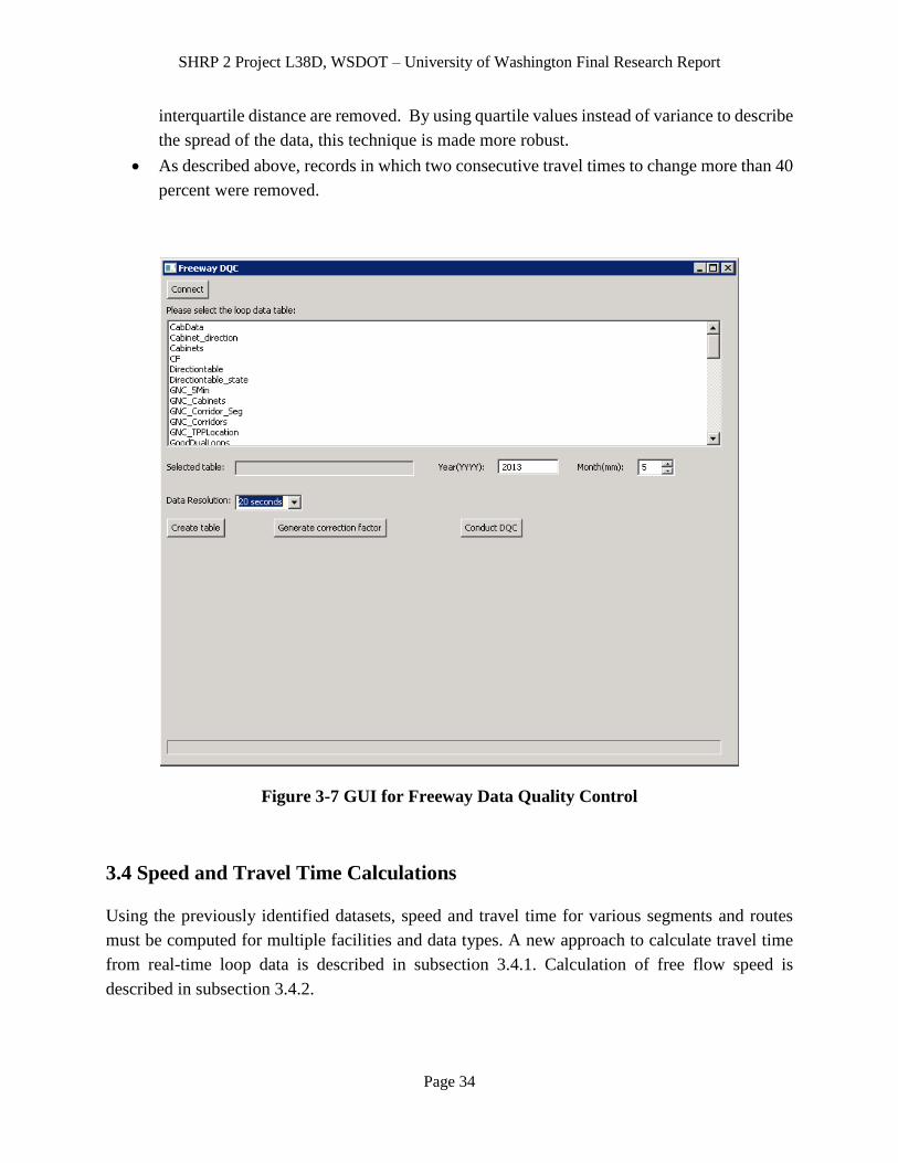
SHRP 2 Project L38D, WSDOT – University of Washington Final Research Report
Page 34
interquartile distance are removed. By using quartile values instead of variance to describe
the spread of the data, this technique is made more robust.
As described above, records in which two consecutive travel times to change more than 40
percent were removed.
Figure 3-7 GUI for Freeway Data Quality Control
3.4 Speed and Travel Time Calculations
Using the previously identified datasets, speed and travel time for various segments and routes
must be computed for multiple facilities and data types. A new approach to calculate travel time
from real-time loop data is described in subsection 3.4.1. Calculation of free flow speed is
described in subsection 3.4.2.

SHRP 2 Project L38D, WSDOT – University of Washington Final Research Report
Page 35
3.4.1 A Travel-Based Approach to Calculating Travel Time from Single Loop Detector Data
For testing the SHRP 2 products, route-level travel time data are needed. The research team
developed a new approach to calculate travel time from single loop data as described below.
In many locations, single loop detectors are one of the most convenient data sources for travel time
calculation. They collect volume and occupancy data that can be converted to an average speed.
By dividing the distance between detectors by the average speed, segment travel times can be
calculated. From here, the simplest and most common way to calculate a route travel time at a
specific time is to calculate all of the segment travel times along the route at that time the route
starts and sum them together to get the route travel time. This method requires minimal calculation
effort, and is often very accurate when the level of congestion remains stable. However, when the
level of congestion changes quickly, the predicted segment travel times at the end of the route will
be quite inaccurate. The travel-based approach described in this section aims to address this
shortcoming.
The first step in calculating a travel-based route travel time begins with the raw data from single
loop detectors. These detectors measure volume and occupancy in each lane which can then be
converted to a speed using the g-factor formula (Equation 3-1).
1flowSpeed
occupancy g (3-1)
The g-factor is a parameter based on the average length of vehicles passing over the detector, and
generally ranges from 2.0-2.5. Before calculating travel times, the average vehicle length for a
route should be studied and an appropriate g-factor should be chosen. Since the travel time
calculation relies on spot speeds, a greater density of detectors along a route will yield more
accurate travel times. At minimum, the density should be greater than one per mile, but a density
closer two per mile is preferable. Once speeds have been determined for each lane, they can be
averaged together at each location. If an HOV lane exists, it should be excluded from this average
in order to get the travel time for general vehicles. Quality control procedures can then be applied
to the speed data. For this study, the following procedures were used, adopted from WSDOT travel
time calculation methods:
If occupancy is less than 12 percent, the speed is set to 60 mph
If occupancy is greater than 95 percent the speed is set to 0 mph
If the calculated speed is less than 10 mph it is set to 10 mph
If the calculated speed is greater than 60 mph it is set to 60 mph
After cleaning up the data, the segment travel time between two adjacent detectors can then be
calculated by taking the distance between the detectors and dividing them by the average of the

SHRP 2 Project L38D, WSDOT – University of Washington Final Research Report
Page 36
speeds they record (Equation 3-2). This result will be referred to as the segment travel time. Once
these segment travel times have been calculated, they can be summed together over large distances
to obtain the travel time for entire routes or corridors.
𝑆𝑒𝑔𝑚𝑒𝑛𝑡 𝑇𝑟𝑎𝑣𝑒𝑙 𝑇𝑖𝑚𝑒 (𝑚𝑖𝑛) = 60 ∗𝑀𝑃2−𝑀𝑃1
(𝑆1+𝑆2)/2 (3-2)
where: MP = Milepost of the detector, S = Speed from detector in mph
As mentioned earlier, the simplest and most common way to calculate a travel time at a specific
moment is to calculate all of the segment travel times along the route (using Equations 3-1 and 3-
2) at that time and sum them together to get the route travel time. However, this method often
yields travel times that vary significantly from ground truth times when a route’s congestion is in
flux (especially on either end of peak travel periods). To overcome this problem, when calculating
travel times from previously collected data (as opposed to real time results) the segment travel
times can be calculated when vehicles actually reach that segment, rather than when they begin
the route. This is clarified by an example below. Consider Table 3-10, which lists segment travel
times (STT) for eight segments and how they change over a 25-minute period as congestion
increases.
Table 3-10: Segment Travel Time Table for Example Route
Time STT 1-2 STT 2-3 STT 3-4 STT 4-5 STT 5-6 STT 6-7 STT 7-8 STT 8-9
3:50 p.m. 1.8 2.0 2.2 4.4 4.6 1.8 2.0 4.2
3:55 p.m. 2.0 2.2 2.4 4.6 4.8 2.0 2.2 4.4
4:00 p.m. 2.2 2.4 2.6 4.8 5.0 2.2 2.4 4.6
4:05 p.m. 2.4 1.6 2.8 5.0 4.2 2.4 2.6 4.8
4:10 p.m. 2.6 1.8 2.0 5.2 4.4 2.6 2.8 4.9
4:15 p.m. 1.8 2 2.2 4.4 4.6 2.8 3 5.2
Using the simple method, the calculated travel time for a vehicle beginning this route at 3:50 p.m.
would be the sum of the first row of the table: 23 minutes. However, using the travel-based method,
the travel time for a vehicle starting at 3:50 p.m. would be calculated as follows. Segment 1-2 is
completed in 1.8 minute, which is before 3:55 p.m.. Thus, segment 2-3 is assumed to be completed
in 2.0 minute. The elapsed time is still before 3:55, and segment 3-4 is assumed to be completed
in 2.2 minute for a running total of 6 minutes. Now the elapsed time is between 3:55 and 4:00, so
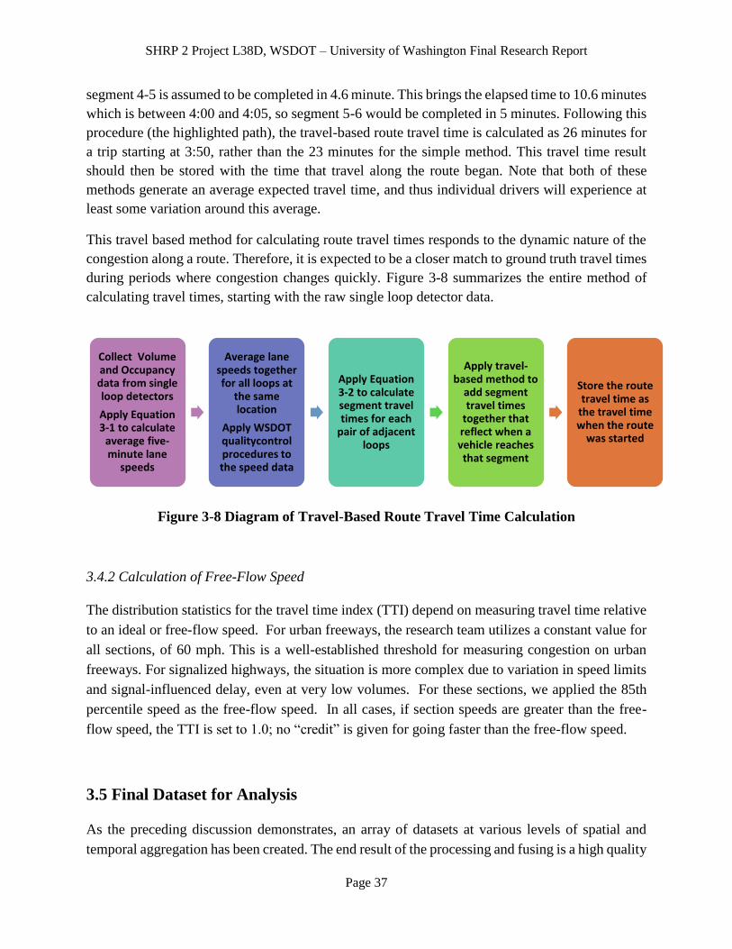
SHRP 2 Project L38D, WSDOT – University of Washington Final Research Report
Page 37
segment 4-5 is assumed to be completed in 4.6 minute. This brings the elapsed time to 10.6 minutes
which is between 4:00 and 4:05, so segment 5-6 would be completed in 5 minutes. Following this
procedure (the highlighted path), the travel-based route travel time is calculated as 26 minutes for
a trip starting at 3:50, rather than the 23 minutes for the simple method. This travel time result
should then be stored with the time that travel along the route began. Note that both of these
methods generate an average expected travel time, and thus individual drivers will experience at
least some variation around this average.
This travel based method for calculating route travel times responds to the dynamic nature of the
congestion along a route. Therefore, it is expected to be a closer match to ground truth travel times
during periods where congestion changes quickly. Figure 3-8 summarizes the entire method of
calculating travel times, starting with the raw single loop detector data.
Figure 3-8 Diagram of Travel-Based Route Travel Time Calculation
3.4.2 Calculation of Free-Flow Speed
The distribution statistics for the travel time index (TTI) depend on measuring travel time relative
to an ideal or free-flow speed. For urban freeways, the research team utilizes a constant value for
all sections, of 60 mph. This is a well-established threshold for measuring congestion on urban
freeways. For signalized highways, the situation is more complex due to variation in speed limits
and signal-influenced delay, even at very low volumes. For these sections, we applied the 85th
percentile speed as the free-flow speed. In all cases, if section speeds are greater than the free-
flow speed, the TTI is set to 1.0; no “credit” is given for going faster than the free-flow speed.
3.5 Final Dataset for Analysis
As the preceding discussion demonstrates, an array of datasets at various levels of spatial and
temporal aggregation has been created. The end result of the processing and fusing is a high quality
Collect Volume and Occupancy data from single loop detectors
Apply Equation 3-1 to calculate
average five-minute lane
speeds
Average lane speeds together for all loops at
the same location
Apply WSDOT qualitycontrol procedures to the speed data
Apply Equation 3-2 to calculate segment travel times for each
pair of adjacent loops
Apply travel-based method to
add segment travel times
together that reflect when a vehicle reaches that segment
Store the route travel time as
the travel time when the route
was started

SHRP 2 Project L38D, WSDOT – University of Washington Final Research Report
Page 38
preprocessed data set to be used in the analyses. A relatively high level of aggregation is required
because reliability is defined over a long period of time to allow all pertinent factors to exert
influence on it. Each observation in the analysis data set is for an individual section for an entire
year for each of the daily time slices studied: peak hour, peak period, mid-day, weekday, and
weekend/holiday. Dataset characteristics under consideration include the following attributes that
are intended to capture characteristics for an entire year on the study sections:
Reliability Metrics
o Mean, standard deviation, median, mode, minimum, and percentiles (10th, 80th,
95th, and 99th) for both travel time and travel time index.
o Buffer indices (based on mean and median), planning time index, skew statistic,
and misery index.
o On-time percentages for thresholds of: median plus 10 percent, median plus 25
percent; and average speeds of 30 mph, 45 mph, and 50 mph.
Operations Characteristics
o Area-wide and section-level service patrol trucks (average number of patrol trucks
per day).
o Area-wide and section-level service patrol trucks per mile (average number of
patrol trucks per day divided by centerline mile).
o Traffic Incident Management Self-Assessment scores.
o Quick clearance law (yes/no).
o Property damage only move-to-shoulder law (yes/no).
o Able to move fatalities without medical examiner (yes/no).
o IRT staff per mile covered.
o Number of ramp meters, DMSs, and CCTVs.
Capacity and Volume Characteristics
o Start and end times for the peak hour and the peak period.
o Calculated and imputed VMT.
o Demand-to-capacity and AADT-to-capacity ratios:
o Average of all links on the section
o Highest for all links on the section
o AADT-to-capacity ratios for downstream bottlenecks as segregated by ramp merge
area.
Incident Characteristics
o Number of incidents (annual).
o Incident rate per 100 million vehicle-miles.
o Incident lane-hours lost (annual).
o Incident shoulder-hours lost (annual).
o Mean, standard deviation, and 95th percentile of incident duration.

SHRP 2 Project L38D, WSDOT – University of Washington Final Research Report
Page 39
Work Zone Characteristics
o Number of work zones (annual).
o Work zone lane-hours lost (annual).
o Work zone shoulder-hours lost (annual).
o Mean, standard deviation, and 95th percentile of work zone duration.
Weather Characteristics
o Number of annual hours with precipitation amounts greater than or equal to 0.01
inches, 0.05 inches, 0.10 inches, 0.25 inches, and 0.50 inches.
o Number of annual hours with measurable snow.
o Number of annual hours with frozen precipitation.
o Number of annual hours with fog present.
3.6 Data Acquisition and Integration
As described in the previous subsections, several sizable data sets from a variety of sources were
archived for this project. To address the challenges of integrating and fusing these diverse data
sets, the STAR Lab DRIVE Net platform is used as a data repository, visualization, and analysis
tool. Figure 3-9 shows an interface snapshot of DRIVE Net Version 3.0.
DRIVE Net is an online e-science platform for data access, analysis, visualization, and quality
control, and is already home to a great deal of public and private transportation data. In addition
to its utility as a data storage and integration tool, DRIVE Net was applied in employed in both
analysis and visualization roles at various stages of this project. DRIVE Net is currently housing
multiple data sources through various methods of data retrieval, for example, traditional flat file
exchange, passive data retrieval, active data retrieval and direct data archival. A variety of data
sources are digested and archived into the STAR Lab server from WSDOT and third party data
providers through different data acquisition methods, as depicted in Figure 3-10.
All of the aforementioned data quality procedures are implemented in the DRIVE Net system,
allowing analysts access to a variety of high quality data sources in an integrated environment.
Quality control is performed on data before it is made available on the platform, removing the need
for substantial preprocessing work and providing a high level of confidence for researchers and
practitioners.
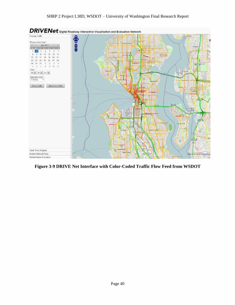
SHRP 2 Project L38D, WSDOT – University of Washington Final Research Report
Page 40
Figure 3-9 DRIVE Net Interface with Color-Coded Traffic Flow Feed from WSDOT
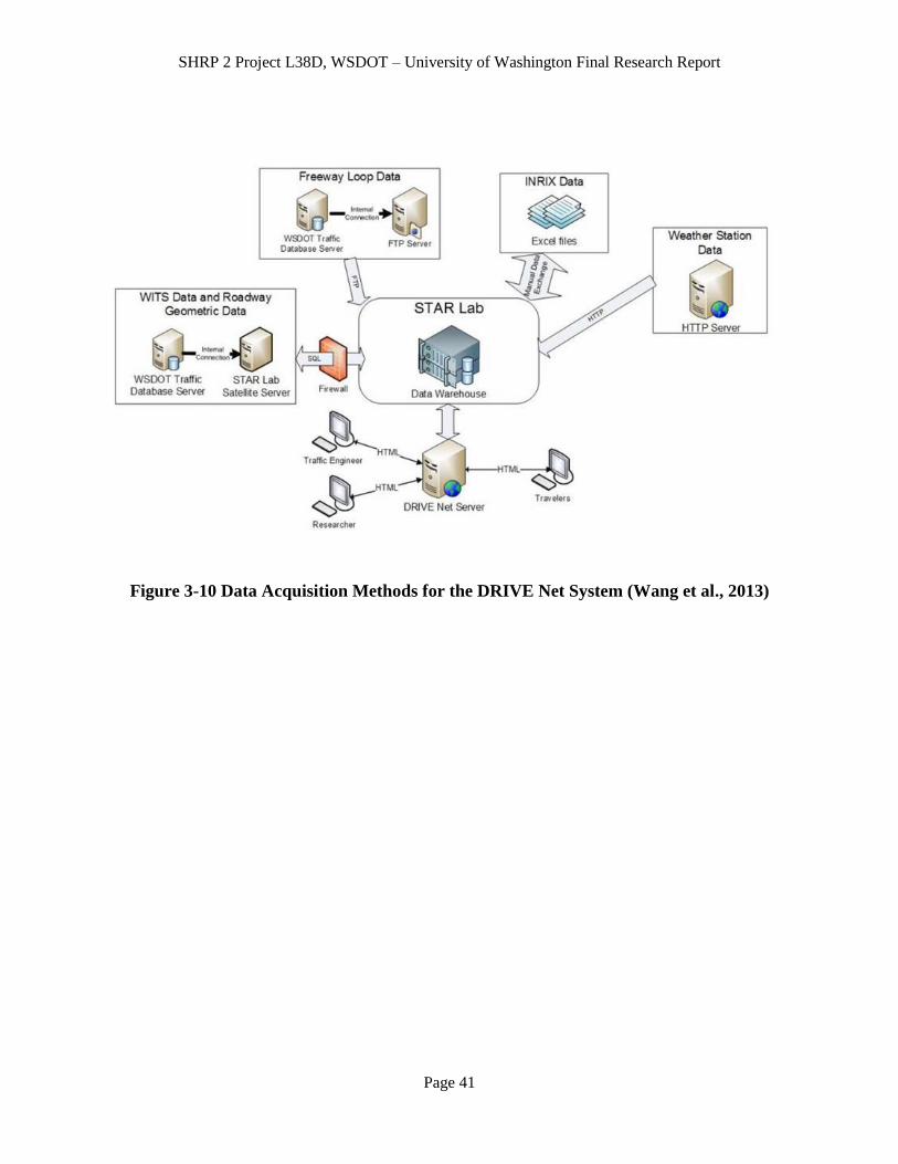
SHRP 2 Project L38D, WSDOT – University of Washington Final Research Report
Page 41
Figure 3-10 Data Acquisition Methods for the DRIVE Net System (Wang et al., 2013)

SHRP 2 Project L38D, WSDOT – University of Washington Final Research Report
Page 42
CHAPTER 4 PILOT TESTING AND ANALYSIS ON SHRP 2 L02
PRODUCT
4.1 Introduction
The L02 project aims at developing tools and procedures for creating a system that monitors travel
time reliability and quantifies the impact of varying conditions on the reliability. Ultimately, the
L02 tools are intended to help transportation agencies answer five basic questions:
1. What is the distribution of travel times in their system?
2. How is the distribution affected by recurrent congestion and non-recurring events?
3. How are freeways and arterials performing relative to performance targets set by the agency?
4. Are capacity investments and other improvements really necessary given the current
distribution of travel times?
5. Are operational improvement actions and capacity investments improving the travel times
and their reliability?
The L02 project’s effectiveness at answering each of these questions was evaluated and any
solutions to any shortcomings are recommended. The three L02 products were also tested by
applying them to a travel time reliability monitoring system (TTRMS). The three products tested
include the guide and its methodology, the TTRMS and its effectiveness in monitoring reliability,
and the approach to synthesizing of route-level travel times from segment-level travel times. This
system helps quantify travel time reliability for a relatively large scale network, visualize the
causes of congestion, and identify segments where a performance improvement is desired.
4.2 Test Sites
Test Sites A and B are selected for L02 product testing. Test Site A includes I-5 northbound and
southbound from Lynnwood to Tukwila and Test Site B covers the entirety of I-405 northbound
and southbound. Test Site A runs 26.5 miles between the southern and northern termini of I-405,
and experiences a peak Annual Average Daily Traffic (AADT) of 228,000 vehicles near milepost
163, just south of the I-5/I-90 interchange. Similarly, the I-405 route (Test Site B) is 29.4 miles
long and experiences a peak AADT of 200,000 vehicles near milepost 12, just north of the I-405/I-
90 interchange. These routes are illustrated in Figure 4-1.
Data was not collected for the I-5 Reversible Express Lanes, which on weekdays run southbound
from approximately 5 am to 11:00 am and northbound from approximately 11:15 am to 11:00 pm.
However these time periods are often delayed or modified due to incidents and special events.
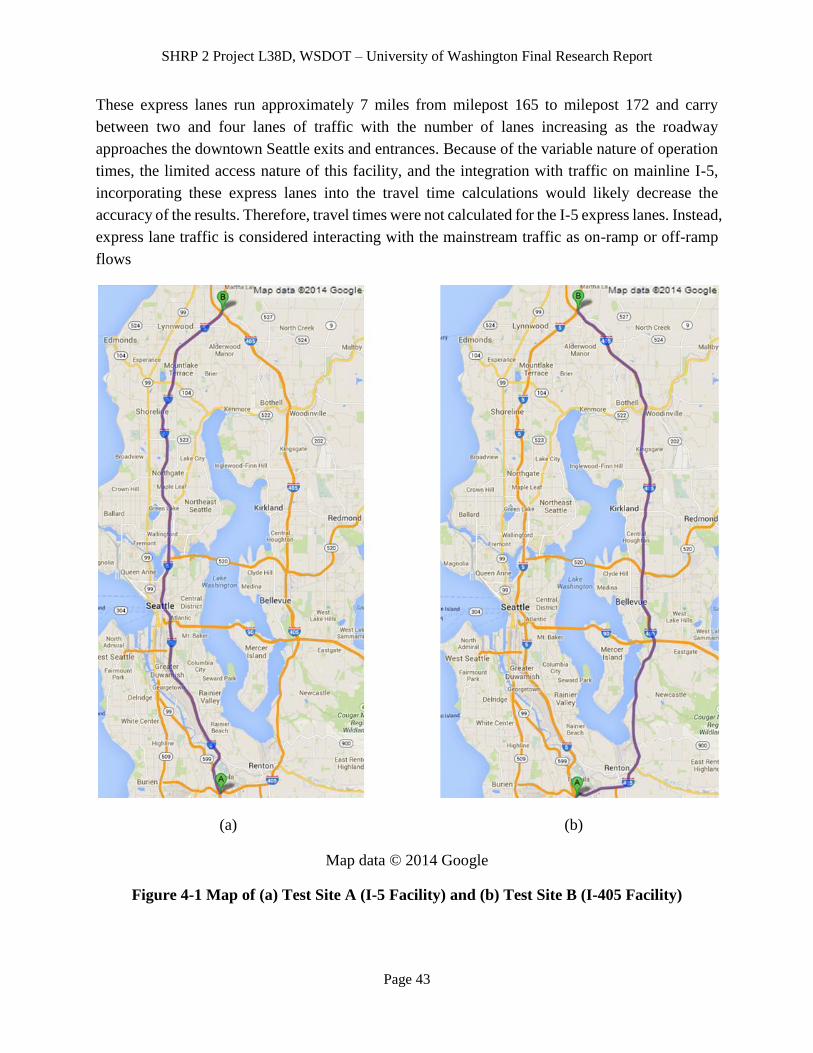
SHRP 2 Project L38D, WSDOT – University of Washington Final Research Report
Page 43
These express lanes run approximately 7 miles from milepost 165 to milepost 172 and carry
between two and four lanes of traffic with the number of lanes increasing as the roadway
approaches the downtown Seattle exits and entrances. Because of the variable nature of operation
times, the limited access nature of this facility, and the integration with traffic on mainline I-5,
incorporating these express lanes into the travel time calculations would likely decrease the
accuracy of the results. Therefore, travel times were not calculated for the I-5 express lanes. Instead,
express lane traffic is considered interacting with the mainstream traffic as on-ramp or off-ramp
flows
(a) (b)
Map data © 2014 Google
Figure 4-1 Map of (a) Test Site A (I-5 Facility) and (b) Test Site B (I-405 Facility)

SHRP 2 Project L38D, WSDOT – University of Washington Final Research Report
Page 44
4.3 Data Description
In this test, 5-minute loop data serve as the basis for the travel time calculations. The procedure
follows the L02 guide for travel time monitoring, in which five-minute interval is stated as the
minimum resolution to accurately capture the effects of weather and incidents on travel time
reliability (TTR). The timeframe of interest is the entire 24-hour day with data from Jan-Dec 2012.
We chose to analyze data for the weekdays of Tuesday through Thursday. Some studies separated
Monday and Friday from other weekdays when predicting traffic patterns, because traffic patterns
during Monday and Friday may deviate from other weekdays. This way, we were able to capture
the most and least congested periods of the day while eliminating the traffic inconsistencies that
are frequently observed on Mondays, Fridays, and weekends. Data from any existing HOV lanes
was also excluded. This single loop data was then converted to speed using Athol’s method (Athol,
1965) with a g-factor of 2.2. The WSDOT travel time estimation methodology specifies the
minimum and maximum speeds to use for travel time calculation. Speeds higher than the
maximum speed are truncated to the maximum speed value of 60 mph. Those lower than the
minimum speed threshold are replaced with the minimum speed of 10 mph. Segment travel times
were then generated by measuring the distance between two adjacent loop locations and dividing
that by the harmonic mean of the speeds measured at these locations. Finally, route-level travel
times are calculated using a piecewise trajectory algorithm that sums the segment-level travel times
along the route.
4.4 Regime Characterization
According to the L02 Guide, a regime is defined as a pair of conditions that consists of a recurring
congestion level and a nonrecurring condition. For the recurring congestion, each travel time
measurement is tagged with a congestion level, i.e., Freeflow, Low, Moderate, and High based on
the time of day and average travel time based on the entire year, as defined in Table 4-1.
Table 4-1 Determination of Congestion Levels for I-5 and I-405
Congestion Level Average Annual Travel Time
Freeflow < 30 min
Low 30-35 min
Moderate 35-40 min
High > 40 min

SHRP 2 Project L38D, WSDOT – University of Washington Final Research Report
Page 45
It is important to note that the times for congestion levels are not determined day to day but rather
reflect the annual average conditions as specified in the L02 Guide.
For the nonrecurring condition, data is tagged as Normal (no nonrecurring event occurred),
Weather (a weather event is occurring that negatively affects traffic), Incident (there is a lane-
blocking incident affecting the study facility), and Overlap (if Weather and Incident occur
simultaneously).
Incidents are tagged using data from the WITS system. Data are tagged as having an incident in
progress if there is an incident blocking a lane or lanes on the route or within 2 miles downstream
of the route, during the five-minute period. Data are tagged as Weather if there is measurable
precipitation during a one-hour period or fog was recorded. The data is taken from local weather
stations, which only reported every hour. Once all data are tagged with a recurring congestion level
and a nonrecurring condition, it could be plotted as a cumulative distribution function (CDF) chart,
the key visual output of the L02 methodology.
4.5 Testing Results and Discussion
After categorizing all the travel time data into the appropriate regimes, many useful charts can be
drawn in analyzing each facility’s travel time reliability and comparing the reliability between the
facilities. The Travel Time Cumulative Distribution Function (CDF) is the key output of L02 and
the most information-rich chart. Figure 4-2 shows each facility’s travel time index CDF (developed
following the L02 procedure).
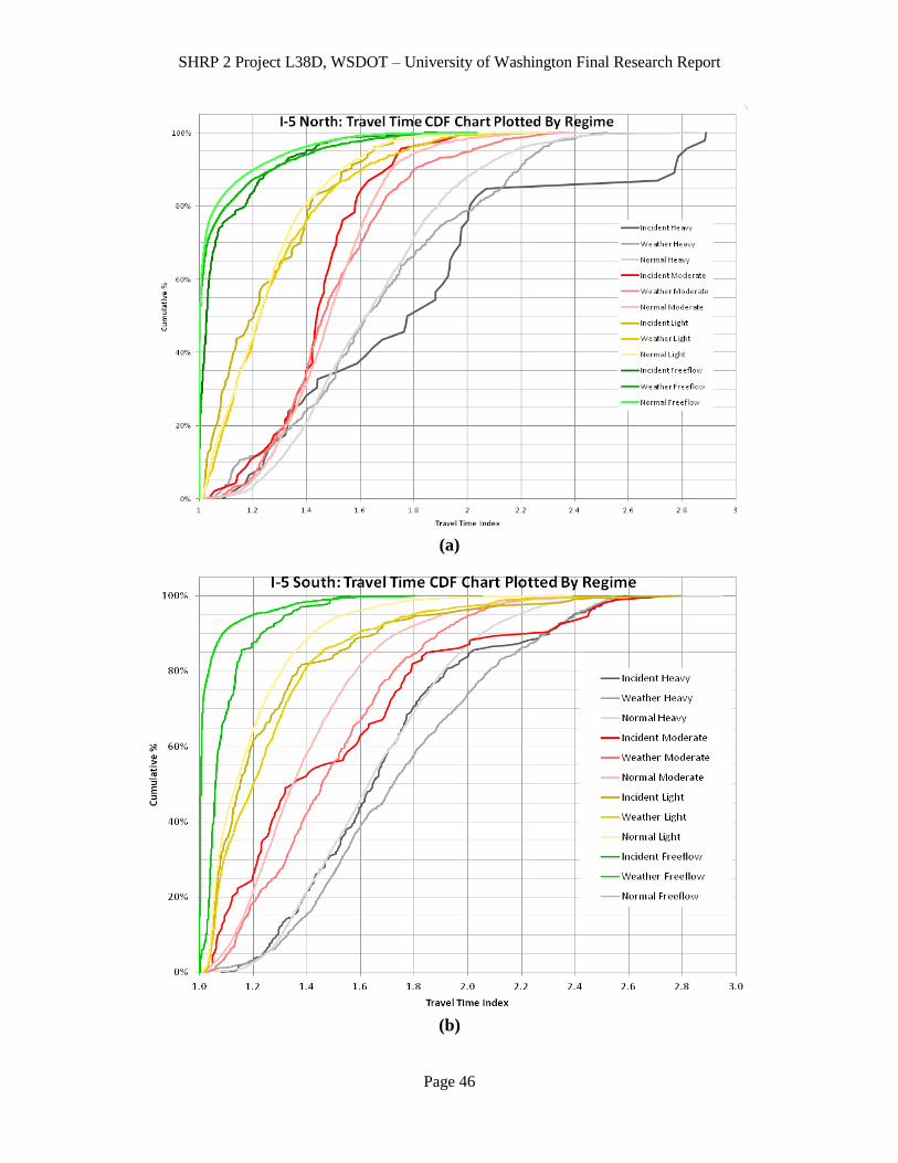
SHRP 2 Project L38D, WSDOT – University of Washington Final Research Report
Page 46
(a)
(b)
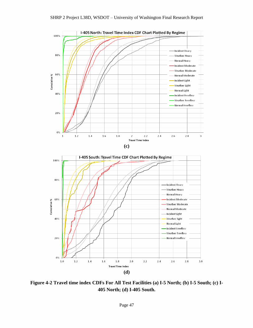
SHRP 2 Project L38D, WSDOT – University of Washington Final Research Report
Page 47
(c)
(d)
Figure 4-2 Travel time index CDFs For All Test Facilities (a) I-5 North; (b) I-5 South; (c) I-
405 North; (d) I-405 South.
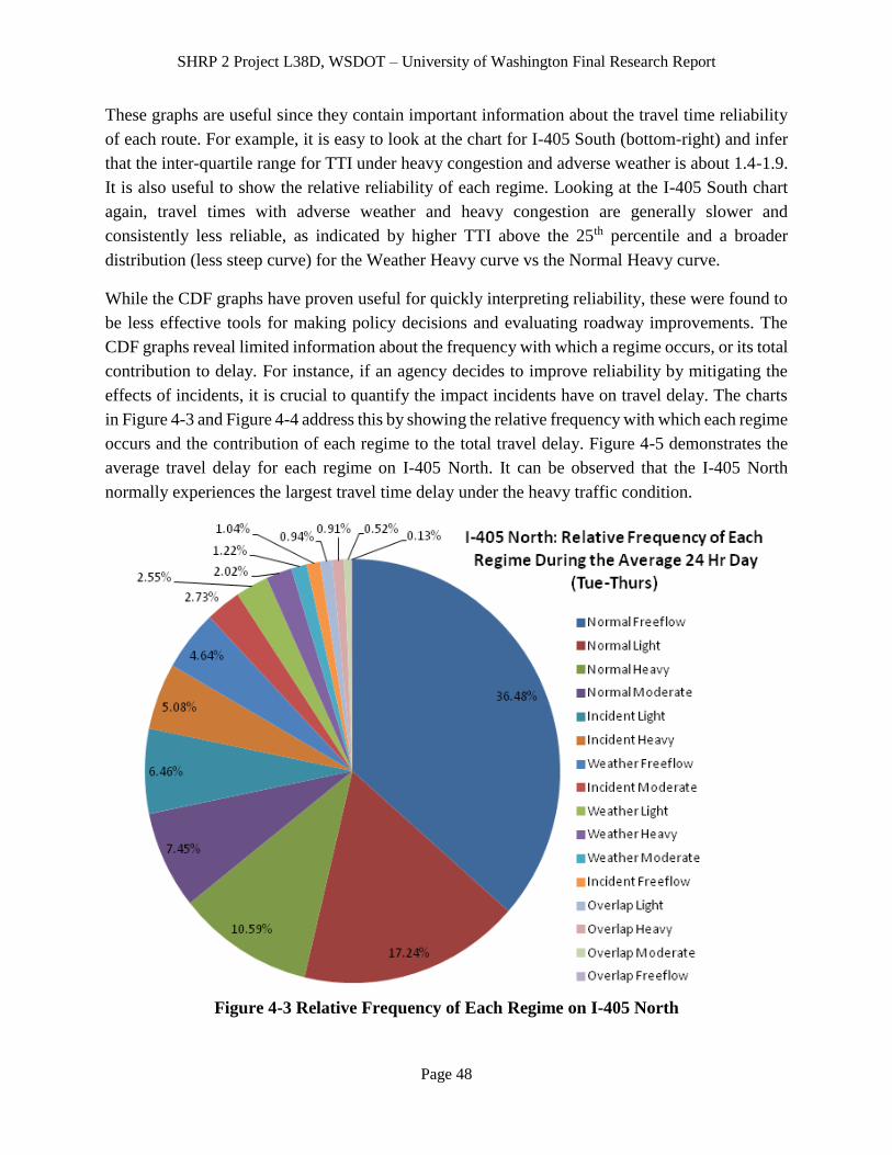
SHRP 2 Project L38D, WSDOT – University of Washington Final Research Report
Page 48
These graphs are useful since they contain important information about the travel time reliability
of each route. For example, it is easy to look at the chart for I-405 South (bottom-right) and infer
that the inter-quartile range for TTI under heavy congestion and adverse weather is about 1.4-1.9.
It is also useful to show the relative reliability of each regime. Looking at the I-405 South chart
again, travel times with adverse weather and heavy congestion are generally slower and
consistently less reliable, as indicated by higher TTI above the 25th percentile and a broader
distribution (less steep curve) for the Weather Heavy curve vs the Normal Heavy curve.
While the CDF graphs have proven useful for quickly interpreting reliability, these were found to
be less effective tools for making policy decisions and evaluating roadway improvements. The
CDF graphs reveal limited information about the frequency with which a regime occurs, or its total
contribution to delay. For instance, if an agency decides to improve reliability by mitigating the
effects of incidents, it is crucial to quantify the impact incidents have on travel delay. The charts
in Figure 4-3 and Figure 4-4 address this by showing the relative frequency with which each regime
occurs and the contribution of each regime to the total travel delay. Figure 4-5 demonstrates the
average travel delay for each regime on I-405 North. It can be observed that the I-405 North
normally experiences the largest travel time delay under the heavy traffic condition.
Figure 4-3 Relative Frequency of Each Regime on I-405 North
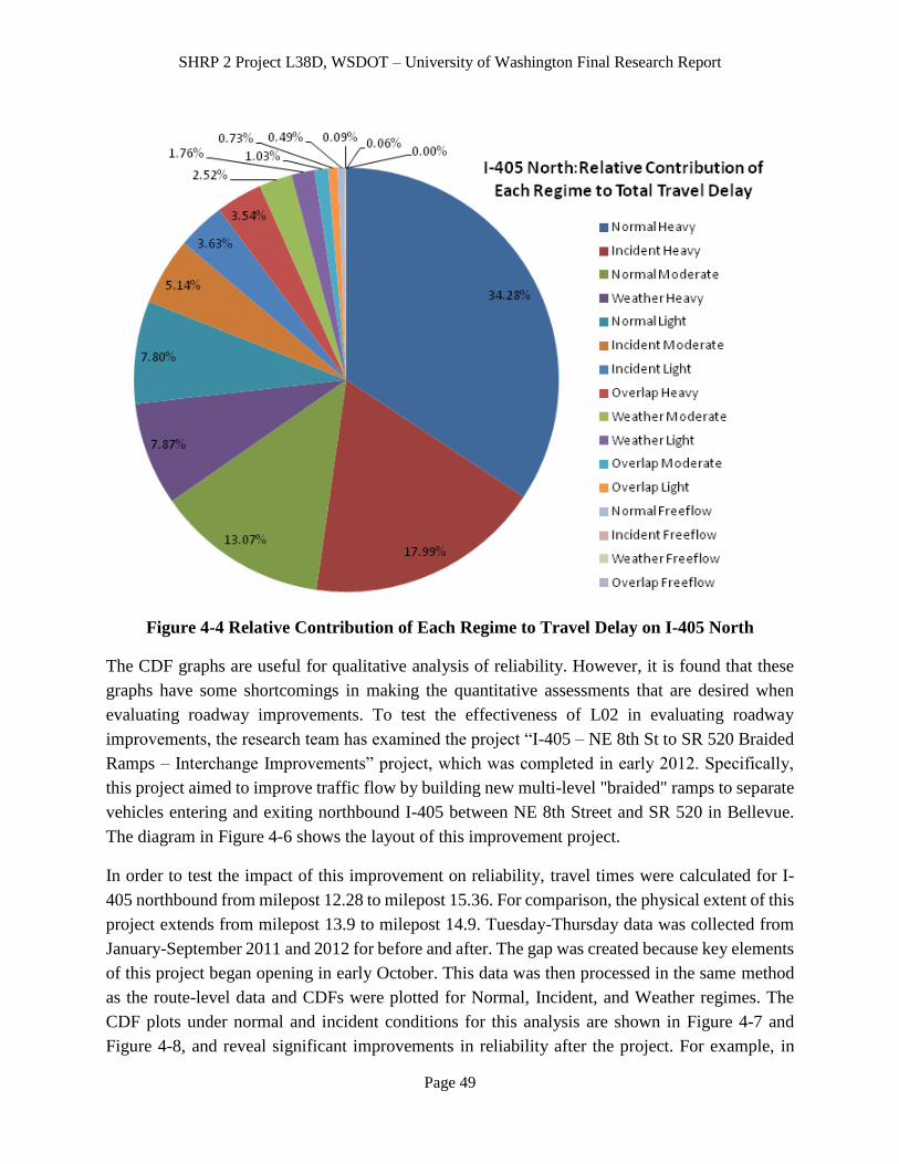
SHRP 2 Project L38D, WSDOT – University of Washington Final Research Report
Page 49
Figure 4-4 Relative Contribution of Each Regime to Travel Delay on I-405 North
The CDF graphs are useful for qualitative analysis of reliability. However, it is found that these
graphs have some shortcomings in making the quantitative assessments that are desired when
evaluating roadway improvements. To test the effectiveness of L02 in evaluating roadway
improvements, the research team has examined the project “I-405 – NE 8th St to SR 520 Braided
Ramps – Interchange Improvements” project, which was completed in early 2012. Specifically,
this project aimed to improve traffic flow by building new multi-level "braided" ramps to separate
vehicles entering and exiting northbound I-405 between NE 8th Street and SR 520 in Bellevue.
The diagram in Figure 4-6 shows the layout of this improvement project.
In order to test the impact of this improvement on reliability, travel times were calculated for I-
405 northbound from milepost 12.28 to milepost 15.36. For comparison, the physical extent of this
project extends from milepost 13.9 to milepost 14.9. Tuesday-Thursday data was collected from
January-September 2011 and 2012 for before and after. The gap was created because key elements
of this project began opening in early October. This data was then processed in the same method
as the route-level data and CDFs were plotted for Normal, Incident, and Weather regimes. The
CDF plots under normal and incident conditions for this analysis are shown in Figure 4-7 and
Figure 4-8, and reveal significant improvements in reliability after the project. For example, in
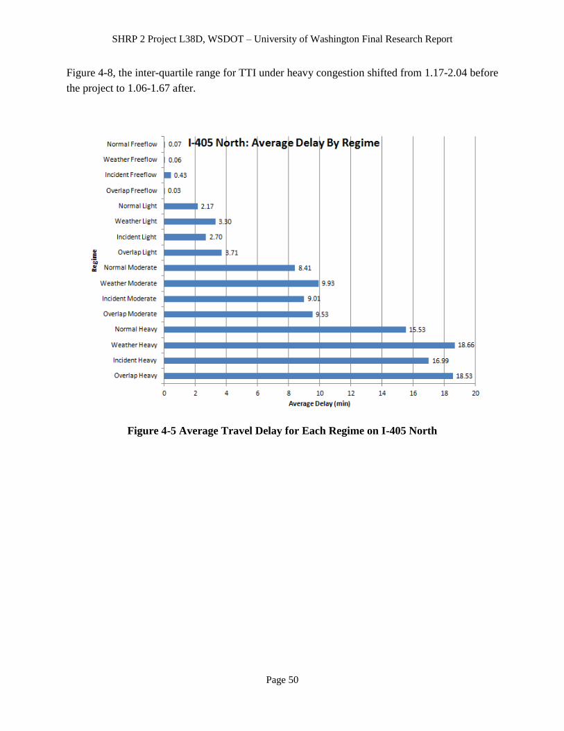
SHRP 2 Project L38D, WSDOT – University of Washington Final Research Report
Page 50
Figure 4-8, the inter-quartile range for TTI under heavy congestion shifted from 1.17-2.04 before
the project to 1.06-1.67 after.
Figure 4-5 Average Travel Delay for Each Regime on I-405 North
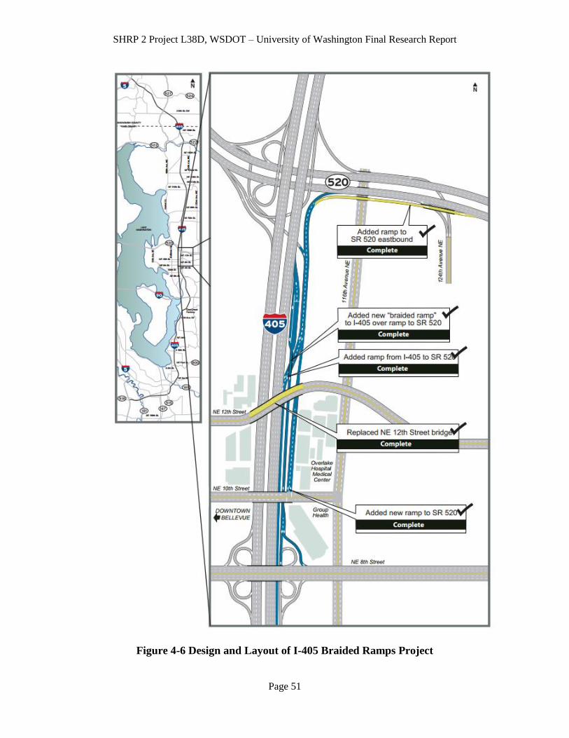
SHRP 2 Project L38D, WSDOT – University of Washington Final Research Report
Page 51
Figure 4-6 Design and Layout of I-405 Braided Ramps Project
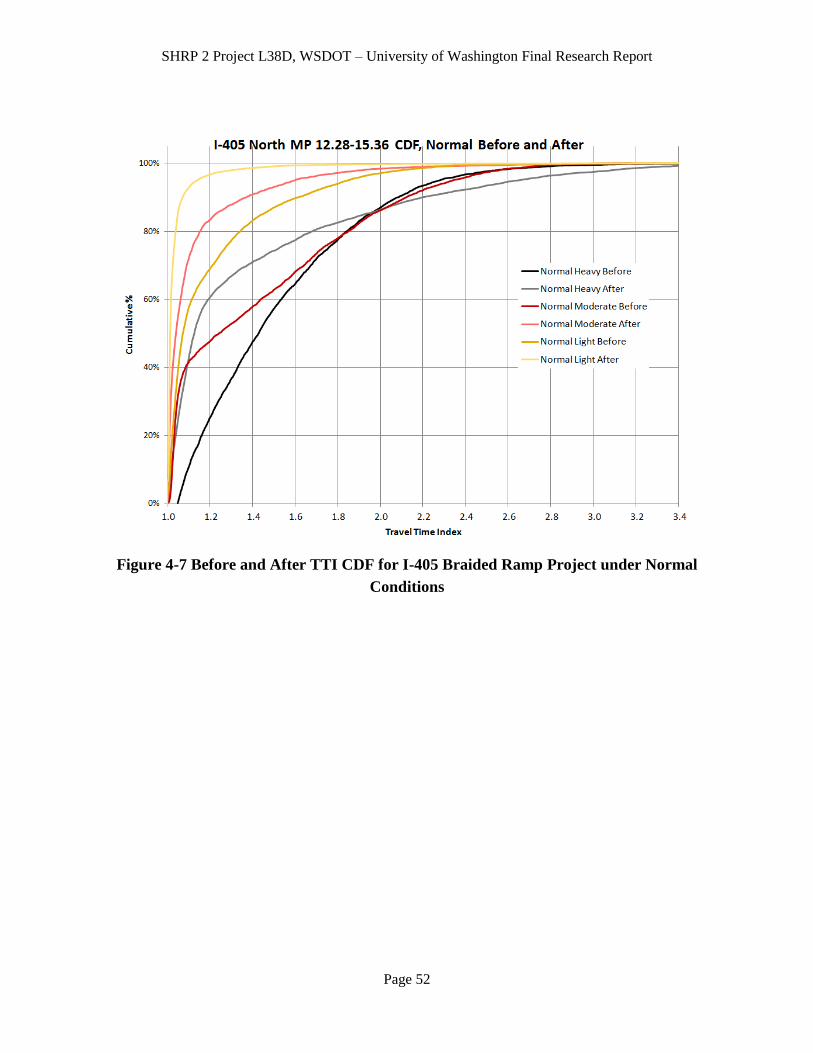
SHRP 2 Project L38D, WSDOT – University of Washington Final Research Report
Page 52
Figure 4-7 Before and After TTI CDF for I-405 Braided Ramp Project under Normal
Conditions
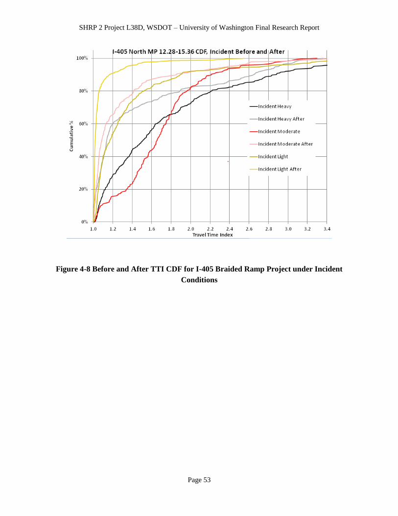
SHRP 2 Project L38D, WSDOT – University of Washington Final Research Report
Page 53
Figure 4-8 Before and After TTI CDF for I-405 Braided Ramp Project under Incident
Conditions

SHRP 2 Project L38D, WSDOT – University of Washington Final Research Report
Page 54
Figure 4-9: TTI Standard Deviations for Each Regime Before and After I-405 Ramp
Project
However, the research team found that the CDF graph makes it somewhat difficult to extract
quantitative values for reliability. In addition, graphing all regimes simultaneously would require
plotting 18 curves on a single graph, which makes the charts less useful. Plotting the standard
deviations by regime as a bar graph was found to be more effective for this application. The results
are shown in Figure 4-9. This graph shows clear reliability improvement in 8 out of 9 regimes,
with only the Normal Heavy regime getting less reliable. An examination of the CDF graph reveals
TTI in this regime actually improved up to the 85th percentile, proving that the CDF is still a
valuable tool for understanding the whole picture.
4.6 Practical Applications of the L02 Methodology
The L02 project’s Travel Time Reliability Monitoring System was implemented on the Digital
Roadway Interactive Visualization and Evaluation Network platform, which is currently being
developed as the WSDOT’s data analytics system. DRIVE Net is a framework for region-wide
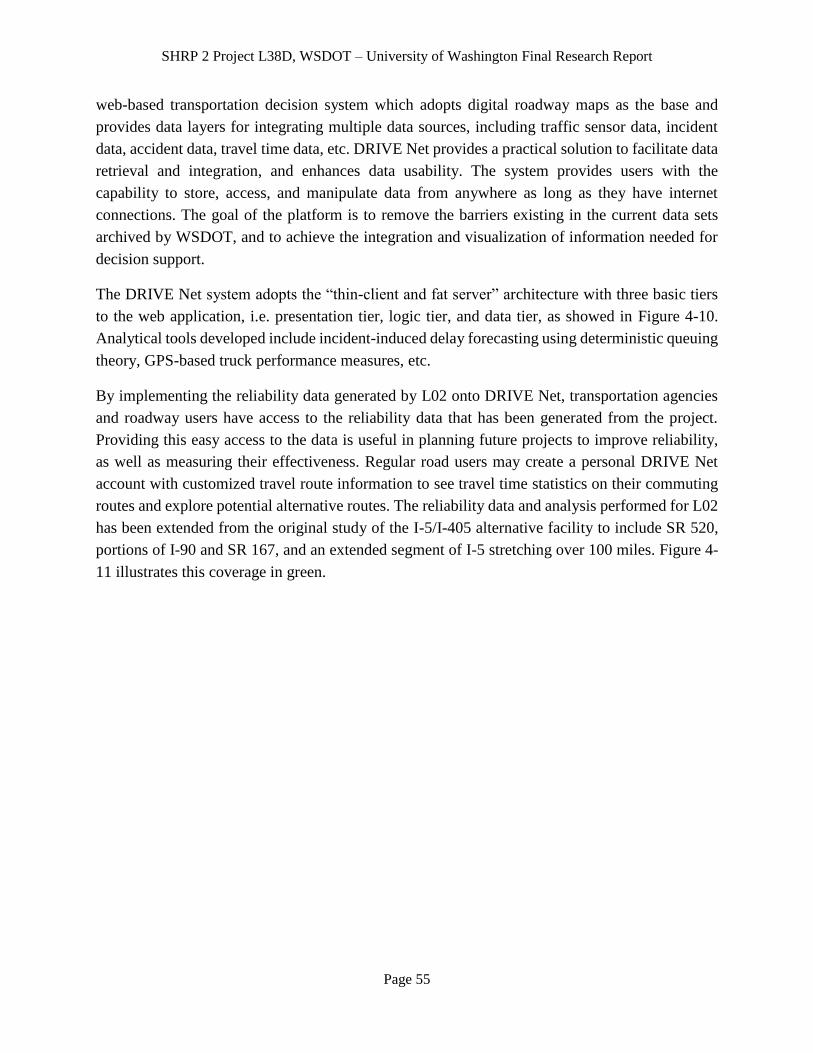
SHRP 2 Project L38D, WSDOT – University of Washington Final Research Report
Page 55
web-based transportation decision system which adopts digital roadway maps as the base and
provides data layers for integrating multiple data sources, including traffic sensor data, incident
data, accident data, travel time data, etc. DRIVE Net provides a practical solution to facilitate data
retrieval and integration, and enhances data usability. The system provides users with the
capability to store, access, and manipulate data from anywhere as long as they have internet
connections. The goal of the platform is to remove the barriers existing in the current data sets
archived by WSDOT, and to achieve the integration and visualization of information needed for
decision support.
The DRIVE Net system adopts the “thin-client and fat server” architecture with three basic tiers
to the web application, i.e. presentation tier, logic tier, and data tier, as showed in Figure 4-10.
Analytical tools developed include incident-induced delay forecasting using deterministic queuing
theory, GPS-based truck performance measures, etc.
By implementing the reliability data generated by L02 onto DRIVE Net, transportation agencies
and roadway users have access to the reliability data that has been generated from the project.
Providing this easy access to the data is useful in planning future projects to improve reliability,
as well as measuring their effectiveness. Regular road users may create a personal DRIVE Net
account with customized travel route information to see travel time statistics on their commuting
routes and explore potential alternative routes. The reliability data and analysis performed for L02
has been extended from the original study of the I-5/I-405 alternative facility to include SR 520,
portions of I-90 and SR 167, and an extended segment of I-5 stretching over 100 miles. Figure 4-
11 illustrates this coverage in green.
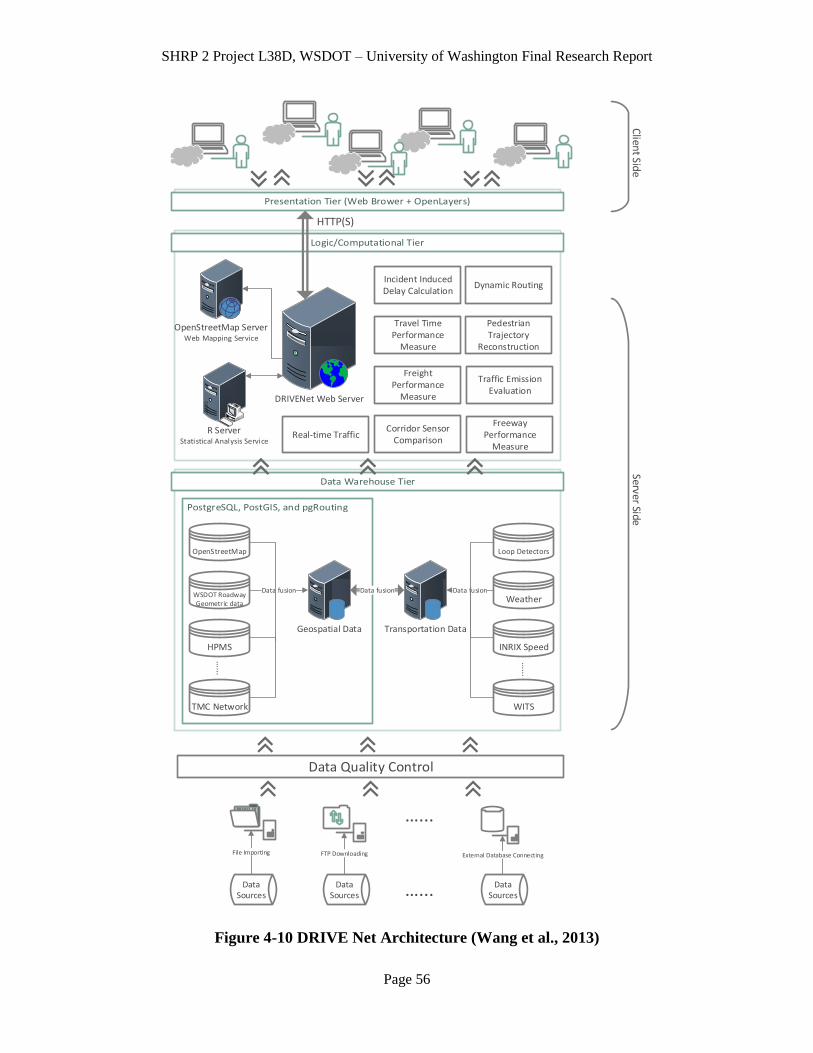
SHRP 2 Project L38D, WSDOT – University of Washington Final Research Report
Page 56
Figure 4-10 DRIVE Net Architecture (Wang et al., 2013)
DRIVENet Web Server
Geospatial Data Transportation Data
Data Sources
Data Quality Control
OpenStreetMap ServerWeb Mapping Service
OpenStreetMap
WSDOT Roadway Geometric data
HPMS
TMC Network
…...
Data fusion
Data Sources
Data Sources
Data fusion
Loop Detectors
Weather
INRIX Speed
WITS
…...
Data fusion
Dynamic RoutingIncident Induced Delay Calculation
Travel Time Performance
Measure
Real-time Traffic
Freight Performance
Measure
Corridor Sensor Comparison
Pedestrian Trajectory
Reconstruction
Traffic Emission Evaluation
Freeway Performance
Measure
Clien
t Side
Server Side
HTTP(S)
R ServerStatistical Analysis Service
File Importing FTP Downloading External Database Connecting
…...
…...
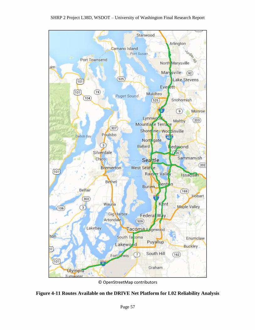
SHRP 2 Project L38D, WSDOT – University of Washington Final Research Report
Page 57
© OpenStreetMap contributors
Figure 4-11 Routes Available on the DRIVE Net Platform for L02 Reliability Analysis

SHRP 2 Project L38D, WSDOT – University of Washington Final Research Report
Page 58
Utilizing this new data, transportation agencies and roadway users can explore reliability anywhere
along these implemented routes, simply by inputting mileposts or clicking on the map. Travel time
reliability information is available in two different forms:
1) Users can directly view the travel times for varying levels of reliability for a custom route
by specifying a starting and ending milepost. A snapshot of this feature is shown in Figure
4-12.
2) Users can specify a starting milepost along with a given amount of travel time and DRIVE
Net can determine how far the user can travel with varying levels of reliability. A snapshot
of this feature is shown in Figure 4-13.
© OpenStreetMap contributors
Figure 4-12: Travel Times for Varying Levels of Reliability for a Custom Route
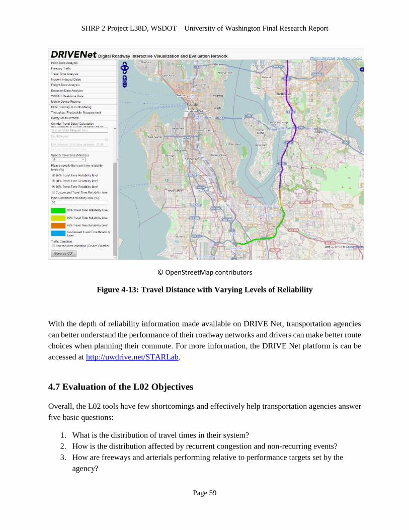
SHRP 2 Project L38D, WSDOT – University of Washington Final Research Report
Page 59
© OpenStreetMap contributors
Figure 4-13: Travel Distance with Varying Levels of Reliability
With the depth of reliability information made available on DRIVE Net, transportation agencies
can better understand the performance of their roadway networks and drivers can make better route
choices when planning their commute. For more information, the DRIVE Net platform is can be
accessed at http://uwdrive.net/STARLab.
4.7 Evaluation of the L02 Objectives
Overall, the L02 tools have few shortcomings and effectively help transportation agencies answer
five basic questions:
1. What is the distribution of travel times in their system?
2. How is the distribution affected by recurrent congestion and non-recurring events?
3. How are freeways and arterials performing relative to performance targets set by the
agency?

SHRP 2 Project L38D, WSDOT – University of Washington Final Research Report
Page 60
4. Are capacity investments and other improvements really necessary given the current
distribution of travel times?
5. Are operational improvement actions and capacity investments improving the travel
times and their reliability?
The distribution of travel times and how it is affected by recurrent congestion and non-recurring
events is clearly and efficiently shown by creating the CDF charts using the L02 methodology.
Comparing performance targets to actual freeway performance is then easily accomplished, as
long as targets are expressed in a way that is compatible with the L02 output. For example,
agencies should express desired performance in terms of performance at various percentiles, or as
the standard deviation of travel time. The need for capacity investments and other improvements
is not perfectly addressed by the L02 tools. The research team felt it was necessary to analyze the
relative contribution of each regime to the overall reliability and delay. This could not be directly
taken from the L02 methods; however it did provide a strong foundation for such analysis. Finally,
the L02 methodology and CDFs were helpful in determining the effectiveness of improvements
and investment. However, it is important to note that L02 specifies route-level analysis, which is
a much larger scale than most improvements. The research team chose to examine improvements
near the segment level, and found that plotting standard deviations of travel times could be more
helpful for detailed analysis.

SHRP 2 Project L38D, WSDOT – University of Washington Final Research Report
Page 61
CHAPTER 5 PILOT TESTING AND ANALYSIS ON SHRP 2 L05
PRODUCT
5.1 Introduction
SHRP 2 L05 provides a concise description of “how-to” incorporate reliability considerations into
the transportation planning and programming process, with a focus on helping agencies make
choices and tradeoffs about funding and project priority.
Through the development of this guide for incorporating reliability into the planning process,
WSDOT, along with the Moving Washington initiative, has been mentioned several times as an
example to illustrate how agencies incorporated the notion of reliability into their policy statements.
From the Gray Notebook, to the Annual Congestion Report, WSDOT has been using different
performance measures to convey reliability trends at corridor and statewide levels. It is without a
doubt that WSDOT has already considered reliability as one of the top priorities in the strategic
planning process.
WSDOT has been in the process of defining an investment philosophy and framework that is
intended to incorporate operational, demand management, and traditional capacity approaches to
produce integrated and incremental corridor investment plans. WSDOT recognizes that
accomplishing this requires the ability to work across organizations and ensure individual program
activities, processes, and expertise are aligned and integrated toward common system performance
objectives and outcomes.
The SHRP 2 L01 (Integrating Business Processes to Improve Reliability) (Kimley-Horn and
Associates, 2011) / L06 (Institutional Architectures to Advance Operational Strategies) (Parsons
Brinckerhoff, & Delcan Corporation, 2012) project focuses on organizational structure and
capabilities associated with integration of reliability and deployment of operational strategies from
a transportation agency perspective. WSDOT was selected as an early implementer and intend to
focus our effort on integrating operations and operational strategies into the planning,
programming, and project development processes. This project has since been refined to focus
specifically on operations program capabilities, processes and products, and the level of maturity
relative to what is necessary to engage effectively in planning processes. Associated with this and
incorporating L05 products would be an assessment of key planning processes to consider how to
incorporate reliability from a performance perspective, and ensure integration of operational and
demand management strategies within planning processes. Performance measurement as it relates
to reliability will be part of this effort. Through this effort, WSDOT intends to identify gaps in
methods, process, organization, and competencies, with the outcome of this effort including the
development of a work plan delineating steps to improve organizational capabilities. The initial

SHRP 2 Project L38D, WSDOT – University of Washington Final Research Report
Page 62
project kick off meeting was held on Oct 29, 2013, with the workshop scheduled for mid-June of
2014.
5.2 SHRP 2 L01/L06 Early Implementation Project
Given that traffic congestion associated with weather, crashes, and special events creates more
than 50 percent of all motorist delay, processes to better manage traffic operations and leverage
existing capacity will make the highway system more reliable and reduce the cost of congestion
for drivers, freight operators, and other users. Several new tools to help agencies advance their
business practices and their organizational structures are now available from SHRP 2. Taken
together, they provide a structure to modernize current practices; mainstream traffic operations in
the state or local department of transportation, and, ultimately, help agencies better plan for and
address non-recurrent congestion on their systems.
A new suite of guides and tools will assist transportation agencies in evaluating and improving
their organizational capabilities to conduct effective and efficient operations. This includes
integrating travel-time reliability into planning, programming, and project delivery processes
while overcoming interdepartmental and interagency barriers to improving highway operations.
The tools for an agency to conduct an assessment of their organizational structure and
business practices for effectiveness in managing travel-time reliability through traffic
operations.
Case studies that show how other states have adjusted their business processes to better
handle traffic incident management, work zone management, and other business functions
related to travel-time reliability.
A system and templates for advancing an agency’s ability to improve systems operations
and management.
The first product, Integrating Business Processes to Improve Travel Time Reliability (L01),
focuses on integrating business processes to allow DOTs to improve reliability through
management of incidents, weather, work zones, special events, traffic control devices, fluctuations
in demand, and bottlenecks.
The second product, Institutional Architectures to Advance Operational Strategies (L06), provides
a comprehensive and systematic examination of ways agencies can be more effectively organized
to successfully execute operations programs that improve travel-time reliability. It includes a self-
evaluation guide, and identifies all the elements needed to improve activities for business processes,
systems and technology, performance management, culture, organization and workforce, and
collaboration.

SHRP 2 Project L38D, WSDOT – University of Washington Final Research Report
Page 63
The focus of this effort will be internal to WSDOT. However, there will be opportunity for MPO
and local agency involvement at various stages of development, such as: at the concept stage as
we refine objectives associated with our Moving Washington framework; and as we develop and
refine strategies, methodologies, processes, and roles necessary to integrate reliability and
operations into to the broader context of overall investment planning.
5.3 SHRP 2 L05 Project Comments
Recognizing that of much of the implementation focus for WSDOT will occur with the deployment
of the L01/L06 Capability and Maturity workshop, a cursory level of review of the “Guide to
Incorporating Reliability Performance Measures into the Transportation Planning and
Programming Processes” was conducted. From this review, WSDOT offers the following
comments:
Overall, the Guide provides a very sound comprehensive approach to incorporating reliability into
planning and programming processes. The descriptions aimed at explaining the various forms the
measure might take, how to communicate the measures in clear understandable terms, and the
significance of the measure as an importance gap filling process to comprehensively considering
system performance was very well presented.
Recognizing that Reliability is a rapidly evolving term, there will be opportunities to continue to
refine how this is presented. These may include:
There are likely limitations to how Reliability can be estimated using existing tools. The
guide suggests existing micro-simulation models as a way that this may be accomplished.
Our experience would indicate that there are challenges with these approaches both from
the level of intensity required to conduct an analysis using these tools, but also from the
potential unknowns that may factor into actual performance. Model calibration would be
a challenge. This would make associating the value of different potential improvement
strategies challenging as well.
Other opportunities for further development could also focus on when in planning horizon
of a facility Reliability and the ability to estimate outcomes of different improvement
alternatives best fit. It seems clear the application and value when considering existing
performance and near term implementation of improvement strategies. How Reliability
can be considered as longer term forecasted and estimated performance measure seems less
clear.
There also seems to be potential for the use of Reliability measures as leading performance
indicators for corridors with emerging congestion. When and how to apply this measure

SHRP 2 Project L38D, WSDOT – University of Washington Final Research Report
Page 64
in developing corridors may provide benefit from the perspective of the timing of when to
begin considering operational strategies ahead of the onset of routine congestion.

SHRP 2 Project L38D, WSDOT – University of Washington Final Research Report
Page 65
CHAPTER 6 PILOT TESTING AND ANALYSIS ON SHRP 2 L07
PRODUCT
6.1 Tool Introduction and Interface
The objective of SHRP 2 L07 is to evaluate the cost-effectiveness of geometric design treatments
in reducing non-recurrent congestion. The L07 products help estimate traffic operational
effectiveness and measure economic benefits of various design treatments. In addition to the
research report, L07 produced an Excel-based software tool to automate the analysis process.
A snapshot of the tool interface is shown in Figure 6-1.
Figure 6-1 SHRP 2 L07 Product Interface
The design treatments considered in the L07 product can be put into four categories as follows:
Shoulder-related treatments
o Accessible Shoulder (for removal of vehicles)
o Alternating Shoulder (for work zones)
o Drivable Shoulder (for diversion of vehicles)

SHRP 2 Project L38D, WSDOT – University of Washington Final Research Report
Page 66
Crash-related treatments
o Crash Investigation Site (urban area)
o Emergency Pull-off (rural area)
o Extra High Median Barrier (eliminate rubbernecking)
o Incident Screen (at the roadside)
Emergency treatments
o Emergency Access (for emergency vehicles)
o Emergency Crossovers (keep open to all vehicles)
o Control (Gated) Turnarounds (used in emergency for all vehicles)
Treatments for special sites
o Runaway Truck Ramp (used in steep downgrade roads)
o Wildlife Crash Reduction
o Anti-icing Systems
o Snow Fence
o Blowing Sand
6.2 Tool Operability
The research team has installed the L07 tool on different operating systems (i.e., 32-bit and 64-bit
Windows 7, 64-bit Windows 8 and the OS X 10.6.8 operation system for Mac computers) with
different versions of Microsoft Office (i.e., Microsoft Office 2010 and Office 2011 for Mac). The
tool can be installed and run successfully for most operating systems. Except for the 64-bit
Windows 8 and the OS X 10.6.8, the installation is unsuccessful and a warning textbook popped
up as shown in Figure 6-2 and Figure 6-3.
In addition, the L07 tool occasionally fails to operate when it was installed on 32-bit and 64-bit
Windows 7. The warning message is shown in Figure 6-4. We found that this run-time error ‘1004’
problem can be solved in Excel 2010 by manually selecting “Trust access to the VBA object model”
and then choosing “Enable all macros” in the Excel’s trust center.
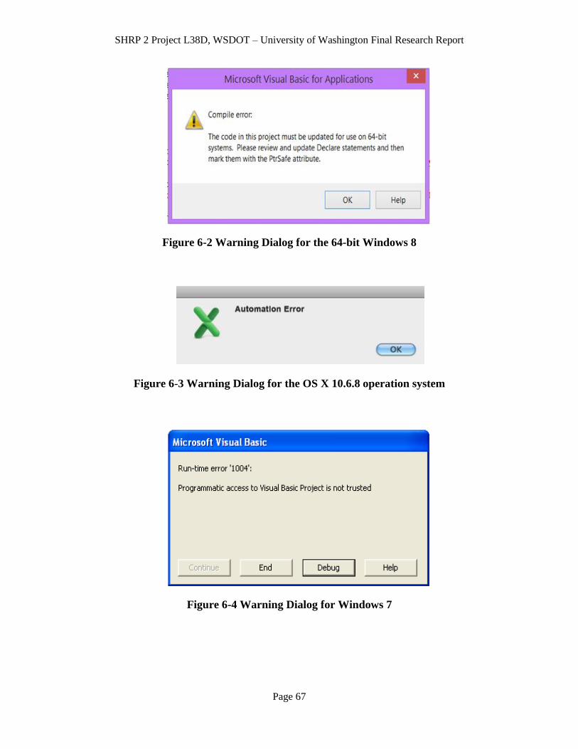
SHRP 2 Project L38D, WSDOT – University of Washington Final Research Report
Page 67
Figure 6-2 Warning Dialog for the 64-bit Windows 8
Figure 6-3 Warning Dialog for the OS X 10.6.8 operation system
Figure 6-4 Warning Dialog for Windows 7
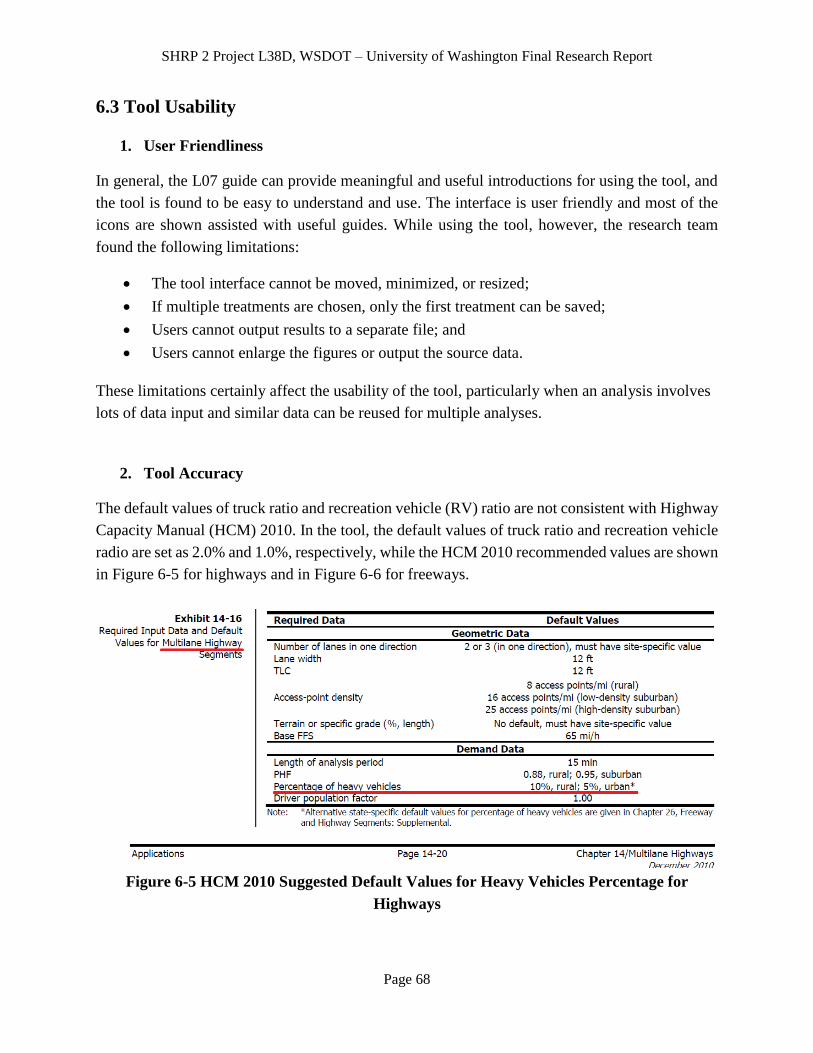
SHRP 2 Project L38D, WSDOT – University of Washington Final Research Report
Page 68
6.3 Tool Usability
1. User Friendliness
In general, the L07 guide can provide meaningful and useful introductions for using the tool, and
the tool is found to be easy to understand and use. The interface is user friendly and most of the
icons are shown assisted with useful guides. While using the tool, however, the research team
found the following limitations:
The tool interface cannot be moved, minimized, or resized;
If multiple treatments are chosen, only the first treatment can be saved;
Users cannot output results to a separate file; and
Users cannot enlarge the figures or output the source data.
These limitations certainly affect the usability of the tool, particularly when an analysis involves
lots of data input and similar data can be reused for multiple analyses.
2. Tool Accuracy
The default values of truck ratio and recreation vehicle (RV) ratio are not consistent with Highway
Capacity Manual (HCM) 2010. In the tool, the default values of truck ratio and recreation vehicle
radio are set as 2.0% and 1.0%, respectively, while the HCM 2010 recommended values are shown
in Figure 6-5 for highways and in Figure 6-6 for freeways.
Figure 6-5 HCM 2010 Suggested Default Values for Heavy Vehicles Percentage for
Highways
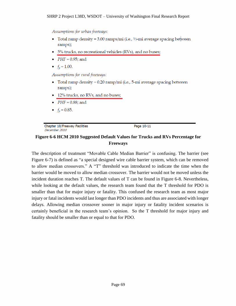
SHRP 2 Project L38D, WSDOT – University of Washington Final Research Report
Page 69
Figure 6-6 HCM 2010 Suggested Default Values for Trucks and RVs Percentage for
Freeways
The description of treatment “Movable Cable Median Barrier” is confusing. The barrier (see
Figure 6-7) is defined as “a special designed wire cable barrier system, which can be removed
to allow median crossovers.” A “T” threshold was introduced to indicate the time when the
barrier would be moved to allow median crossover. The barrier would not be moved unless the
incident duration reaches T. The default values of T can be found in Figure 6-8. Nevertheless,
while looking at the default values, the research team found that the T threshold for PDO is
smaller than that for major injury or fatality. This confused the research team as most major
injury or fatal incidents would last longer than PDO incidents and thus are associated with longer
delays. Allowing median crossover sooner in major injury or fatality incident scenarios is
certainly beneficial in the research team’s opinion. So the T threshold for major injury and
fatality should be smaller than or equal to that for PDO.
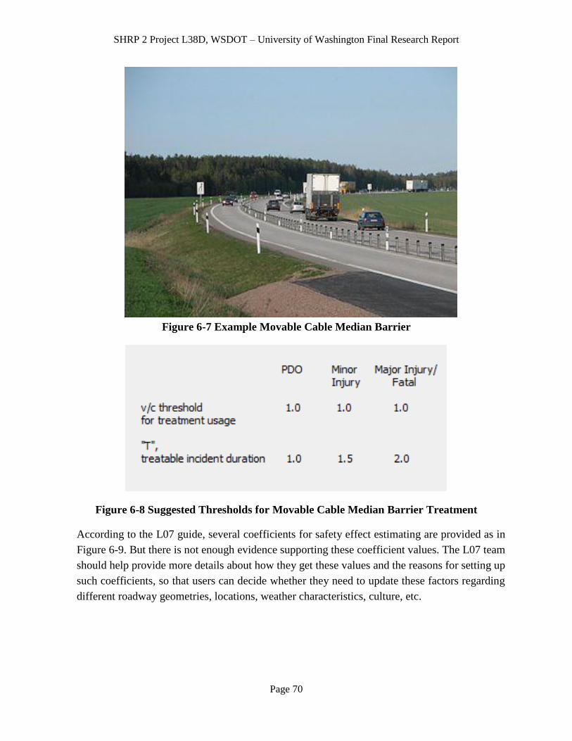
SHRP 2 Project L38D, WSDOT – University of Washington Final Research Report
Page 70
Figure 6-7 Example Movable Cable Median Barrier
Figure 6-8 Suggested Thresholds for Movable Cable Median Barrier Treatment
According to the L07 guide, several coefficients for safety effect estimating are provided as in
Figure 6-9. But there is not enough evidence supporting these coefficient values. The L07 team
should help provide more details about how they get these values and the reasons for setting up
such coefficients, so that users can decide whether they need to update these factors regarding
different roadway geometries, locations, weather characteristics, culture, etc.

SHRP 2 Project L38D, WSDOT – University of Washington Final Research Report
Page 71
Figure 6-9 Suggested Default Coefficients in L07 Guide

SHRP 2 Project L38D, WSDOT – University of Washington Final Research Report
Page 72
6.4 Performance Test
Testing of L07 tool performance is conducted in three folds: 1) a comparison study is made with
the DRIVE Net system to test the measure of effectiveness (MOE) sub-output; 2) a comparison
study is made with on-site single loop detector data to test the tool’s production of the TTI curve
and 3) a case study is conducted to test the benefit-cost sub-output.
1) Output Comparison with DRIVE Net
The key feature of the L07 tool is to estimate the travel time index (TTI) curves both before and
after the design treatment. As the DRIVE Net system can also calculate the same MOE for
WSDOT’s productions of the Gray Notebooks, the research team compared TTI curves produced
by the DRIVE Net and the L07 tool.
Gray Notebook capacity analysis includes a travel time analysis method using both loop and
INRIX data. The procedure for calculating travel time distribution is quite similar to the
methodology recommended by L07. Vehicle average travel time is calculated and updated for each
five minute period. Then the travel time cumulative distribution is summarized for each time slot
in all weekdays throughout the year. The results are more accurate than the travel time estimation
results based solely on the output from loop detector, since travel time is calculated using real-
time vehicle speed collected from GPS devices when possible. Gray Notebook has been published
for many years. The travel time estimates for the selected corridors have been verified through
different means in WSDOT. So the Gray Notebook travel time data is a great benchmark dataset
to compare with calculation results from the SHRP 2 Reliability products.
A Gray Notebooks data source facility within the L07 test sites is an I-5 segment from milepost
184 to milepost 185.5. DRIVE Net computes two sets of TTI for morning peak (8:20 a.m.) and
afternoon peak (5:30 p.m.), respectively. Figure 6-10 shows the outputs of DRIVE Net (left) and
L07 Tool (right).
According to Figure 6-10, it’s difficult to tell whether the L07 tool gives accurate estimation of
the TTI curve because the L07 tool does not allow users to resize/enlarge the output graphs nor
output the source data. However, when looking at the 50 percentile TTI values for the afternoon
period, the research team finds that DRIVE Net reports larger TTI values than those from the L07
tool. Since the selected I-5 facility is very congested during evening peak, and DRIVE Net system
is based on daily data over an entire year (work days), the research team believes that the DRVIVE
Net output is closer to the ground truth.
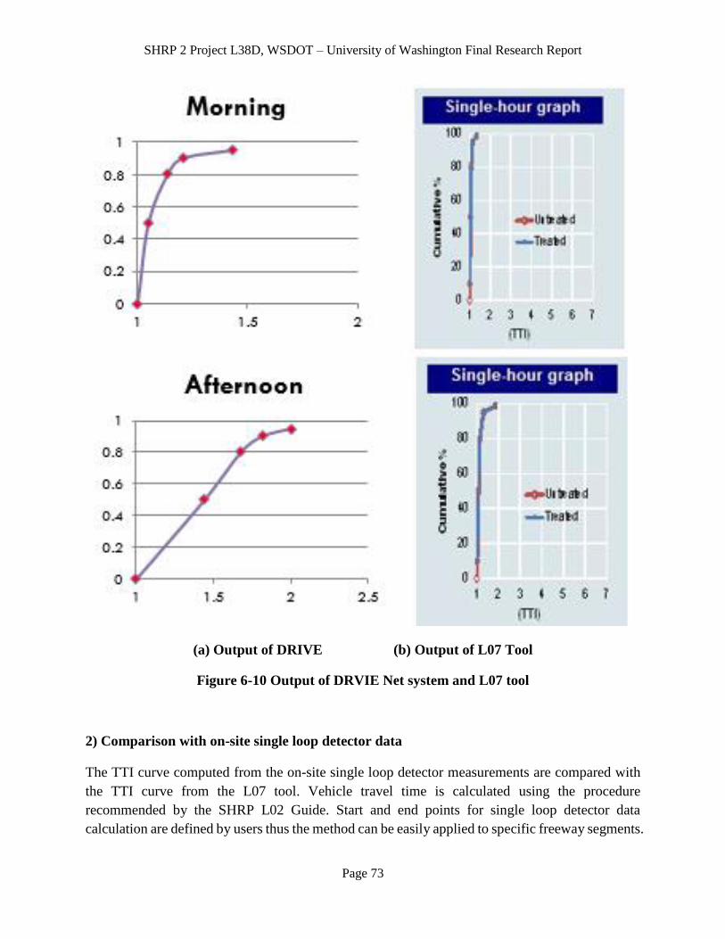
SHRP 2 Project L38D, WSDOT – University of Washington Final Research Report
Page 73
(a) Output of DRIVE (b) Output of L07 Tool
Figure 6-10 Output of DRVIE Net system and L07 tool
2) Comparison with on-site single loop detector data
The TTI curve computed from the on-site single loop detector measurements are compared with
the TTI curve from the L07 tool. Vehicle travel time is calculated using the procedure
recommended by the SHRP L02 Guide. Start and end points for single loop detector data
calculation are defined by users thus the method can be easily applied to specific freeway segments.
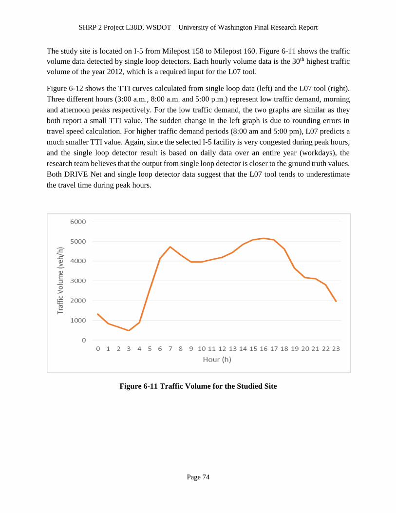
SHRP 2 Project L38D, WSDOT – University of Washington Final Research Report
Page 74
The study site is located on I-5 from Milepost 158 to Milepost 160. Figure 6-11 shows the traffic
volume data detected by single loop detectors. Each hourly volume data is the 30th highest traffic
volume of the year 2012, which is a required input for the L07 tool.
Figure 6-12 shows the TTI curves calculated from single loop data (left) and the L07 tool (right).
Three different hours (3:00 a.m., 8:00 a.m. and 5:00 p.m.) represent low traffic demand, morning
and afternoon peaks respectively. For the low traffic demand, the two graphs are similar as they
both report a small TTI value. The sudden change in the left graph is due to rounding errors in
travel speed calculation. For higher traffic demand periods (8:00 am and 5:00 pm), L07 predicts a
much smaller TTI value. Again, since the selected I-5 facility is very congested during peak hours,
and the single loop detector result is based on daily data over an entire year (workdays), the
research team believes that the output from single loop detector is closer to the ground truth values.
Both DRIVE Net and single loop detector data suggest that the L07 tool tends to underestimate
the travel time during peak hours.
Figure 6-11 Traffic Volume for the Studied Site
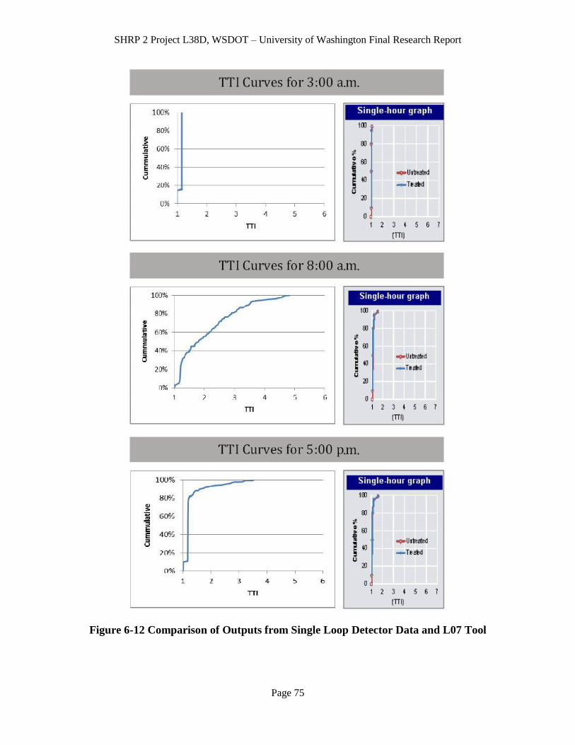
SHRP 2 Project L38D, WSDOT – University of Washington Final Research Report
Page 75
Figure 6-12 Comparison of Outputs from Single Loop Detector Data and L07 Tool
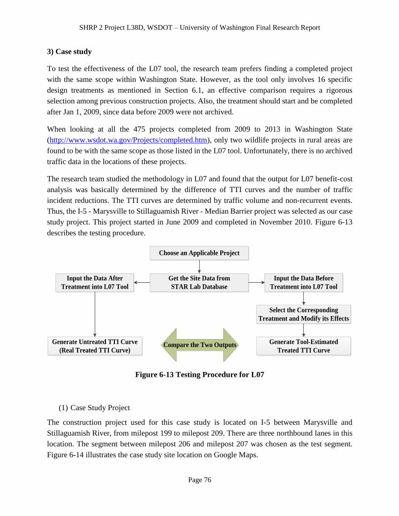
SHRP 2 Project L38D, WSDOT – University of Washington Final Research Report
Page 76
3) Case study
To test the effectiveness of the L07 tool, the research team prefers finding a completed project
with the same scope within Washington State. However, as the tool only involves 16 specific
design treatments as mentioned in Section 6.1, an effective comparison requires a rigorous
selection among previous construction projects. Also, the treatment should start and be completed
after Jan 1, 2009, since data before 2009 were not archived.
When looking at all the 475 projects completed from 2009 to 2013 in Washington State
(http://www.wsdot.wa.gov/Projects/completed.htm), only two wildlife projects in rural areas are
found to be with the same scope as those listed in the L07 tool. Unfortunately, there is no archived
traffic data in the locations of these projects.
The research team studied the methodology in L07 and found that the output for L07 benefit-cost
analysis was basically determined by the difference of TTI curves and the number of traffic
incident reductions. The TTI curves are determined by traffic volume and non-recurrent events.
Thus, the I-5 - Marysville to Stillaguamish River - Median Barrier project was selected as our case
study project. This project started in June 2009 and completed in November 2010. Figure 6-13
describes the testing procedure.
Choose an Applicable Project
Get the Site Data from
STAR Lab Database
Input the Data Before
Treatment into L07 Tool
Select the Corresponding
Treatment and Modify its Effects
Generate Tool-Estimated
Treated TTI Curve
Input the Data After
Treatment into L07 Tool
Generate Untreated TTI Curve
(Real Treated TTI Curve)Compare the Two Outputs
Figure 6-13 Testing Procedure for L07
(1) Case Study Project
The construction project used for this case study is located on I-5 between Marysville and
Stillaguamish River, from milepost 199 to milepost 209. There are three northbound lanes in this
location. The segment between milepost 206 and milepost 207 was chosen as the test segment.
Figure 6-14 illustrates the case study site location on Google Maps.
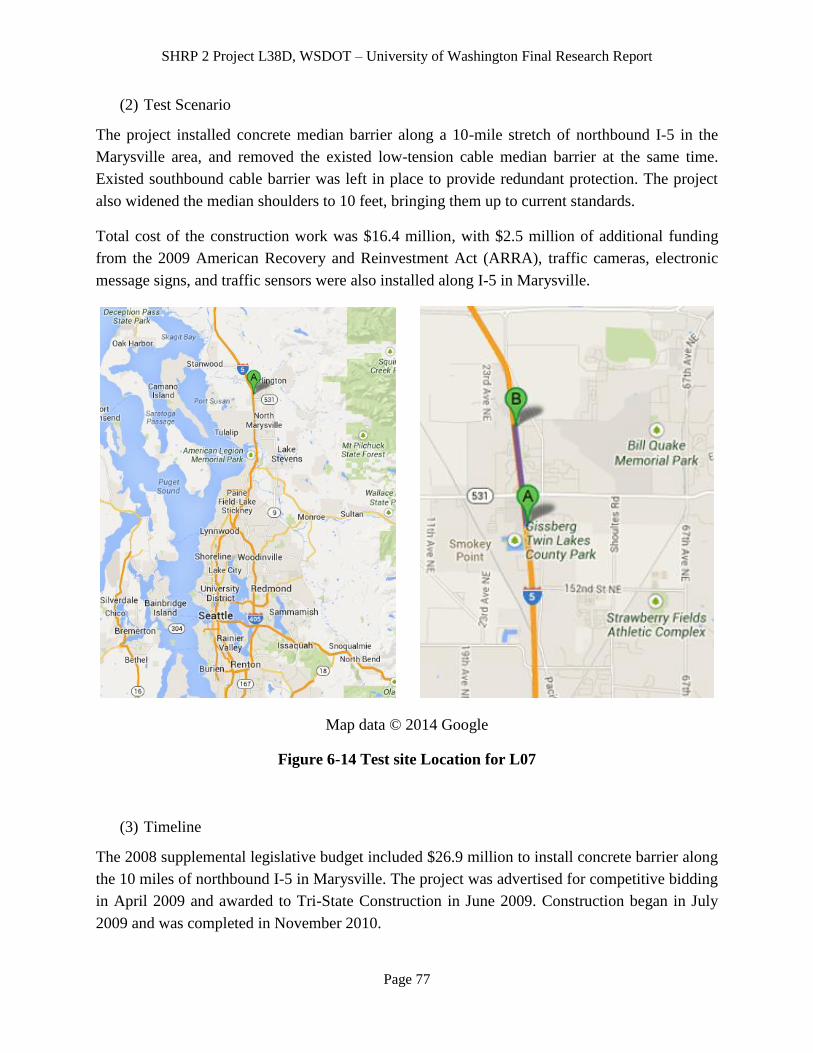
SHRP 2 Project L38D, WSDOT – University of Washington Final Research Report
Page 77
(2) Test Scenario
The project installed concrete median barrier along a 10-mile stretch of northbound I-5 in the
Marysville area, and removed the existed low-tension cable median barrier at the same time.
Existed southbound cable barrier was left in place to provide redundant protection. The project
also widened the median shoulders to 10 feet, bringing them up to current standards.
Total cost of the construction work was $16.4 million, with $2.5 million of additional funding
from the 2009 American Recovery and Reinvestment Act (ARRA), traffic cameras, electronic
message signs, and traffic sensors were also installed along I-5 in Marysville.
Map data © 2014 Google
Figure 6-14 Test site Location for L07
(3) Timeline
The 2008 supplemental legislative budget included $26.9 million to install concrete barrier along
the 10 miles of northbound I-5 in Marysville. The project was advertised for competitive bidding
in April 2009 and awarded to Tri-State Construction in June 2009. Construction began in July
2009 and was completed in November 2010.
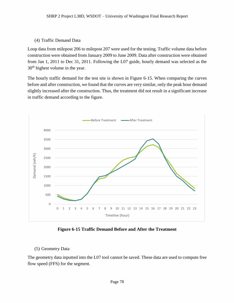
SHRP 2 Project L38D, WSDOT – University of Washington Final Research Report
Page 78
(4) Traffic Demand Data
Loop data from milepost 206 to milepost 207 were used for the testing. Traffic volume data before
construction were obtained from January 2009 to June 2009. Data after construction were obtained
from Jan 1, 2011 to Dec 31, 2011. Following the L07 guide, hourly demand was selected as the
30th highest volume in the year.
The hourly traffic demand for the test site is shown in Figure 6-15. When comparing the curves
before and after construction, we found that the curves are very similar, only the peak hour demand
slightly increased after the construction. Thus, the treatment did not result in a significant increase
in traffic demand according to the figure.
Figure 6-15 Traffic Demand Before and After the Treatment
(5) Geometry Data
The geometry data inputted into the L07 tool cannot be saved. These data are used to compute free
flow speed (FFS) for the segment.
0
500
1000
1500
2000
2500
3000
3500
4000
0 1 2 3 4 5 6 7 8 9 10 11 12 13 14 15 16 17 18 19 20 21 22 23
Dem
and
(ve
h/h
)
Timeline (hour)
Before Treatment After Treatment

SHRP 2 Project L38D, WSDOT – University of Washington Final Research Report
Page 79
(6) Traffic Incident Data
Incidents for the segment can be found from the WITS database. Numbers of different types of
incidents before and after treatment are listed in Table 6-1. Incident numbers before the treatment
are estimated as the average number for 2006 through 2008; incident numbers after the treatments
are estimated as the average number of year 2011 and 2012.
Table 6-1 Incident Numbers for I-5 milepost 199-209
Before After Decrease
Year 2006 2007 2008 Mean 2011 2012 Mean %
Property damaged only 17 23 30 23.3 2 8 5 78.6
Minor Injury 6 3 7 5.3 3 2 2.5 53.1
Fatality 1 1 2 1.3 0 0 0 100
Non-crash 575 625 627 609 136 130 133 78.2
Total 599 652 666 639 141 140 140.5 78.0
Summarizing Table 6-1, the conclusion can be drawn that the treatment had a significantly positive
effect on reducing traffic incidents, especially severe incidents. Looking at the data in Table 6-1,
all kinds of crash-incidents were reduced by 50% or more after the concrete median barrier was
built.
For the tool testing purpose, actual incident numbers for the test site are applied to replace default
values. For crash costs, the default values suggested by the L07 guide are used.
(7) Weather, Event, and Work Zone Data
For weather data, defaults provided by the tool are used. The nearest location to provide the
weather data is selected as Seattle. No event or work zone happened on the segment during the
testing period.
(8) Treatment Selection
In choosing the proper treatment, the research team tried ‘Extra High Med Barrier’ treatment
within the tool first, because the definition of it seems to be the closest to the actual treatment.
However, the ‘Extra High Med Barrier’ treatment in the tool only targets on gawk-inducing
incidents, which only contribute a small proportion to all the incidents. At the same time, if the
input value for incident reduction is close to 100%, the software crashes (see Figure 6-16).
To make the testing more precise, the research team chose another treatment called ‘Anti-icing
Systems’ for the testing. Though the definition of treatment does not close to the actual median
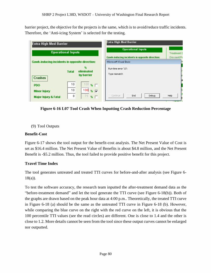
SHRP 2 Project L38D, WSDOT – University of Washington Final Research Report
Page 80
barrier project, the objective for the projects is the same, which is to avoid/reduce traffic incidents.
Therefore, the ‘Anti-icing System’ is selected for the testing.
Figure 6-16 L07 Tool Crash When Inputting Crash Reduction Percentage
(9) Tool Outputs
Benefit-Cost
Figure 6-17 shows the tool output for the benefit-cost analysis. The Net Present Value of Cost is
set as $16.4 million. The Net Present Value of Benefits is about $4.8 million, and the Net Present
Benefit is -$5.2 million. Thus, the tool failed to provide positive benefit for this project.
Travel Time Index
The tool generates untreated and treated TTI curves for before-and-after analysis (see Figure 6-
18(a)).
To test the software accuracy, the research team inputted the after-treatment demand data as the
“before-treatment demand” and let the tool generate the TTI curve (see Figure 6-18(b)). Both of
the graphs are drawn based on the peak hour data at 4:00 p.m.. Theoretically, the treated TTI curve
in Figure 6-18 (a) should be the same as the untreated TTI curve in Figure 6-18 (b). However,
while comparing the blue curve on the right with the red curve on the left, it is obvious that the
100 percentile TTI values (see the read circles) are different. One is close to 1.4 and the other is
close to 1.2. More details cannot be seen from the tool since these output curves cannot be enlarged
nor outputted.
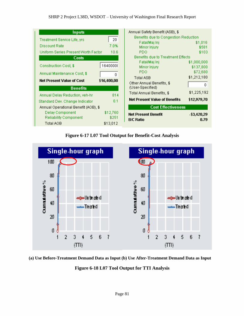
SHRP 2 Project L38D, WSDOT – University of Washington Final Research Report
Page 81
Figure 6-17 L07 Tool Otutput for Benefit-Cost Analysis
(a) Use Before-Treatment Demand Data as Input (b) Use After-Treatment Demand Data as Input
Figure 6-18 L07 Tool Output for TTI Analysis

SHRP 2 Project L38D, WSDOT – University of Washington Final Research Report
Page 82
6.5 Test Conclusions
The research team believes that the L07 methodology on computing TTI curves should be further
studied and compared. Neither the output comparison between L07 and DRIVE Net nor the
software accuracy comparison between L07 “before-treatment” curve (see Figure 6-18 (b), red
curve) and L07 “after-treatment” curve (see Figure 6-18 (a), blue curve) yield a positive conclusion.
At the same time, the research team suggests the L07 project team help revise the tool and allow
the user to obtain more detailed output information from it.
In the L07 tool, the treatment “Extra High Med Barrier” only deals with gawk-inducing incidents.
However, such treatment in reality can also help prevent other types of incidents. For example,
some high concrete median barrier can also prevent vehicles from running into the opposite
direction, so that some severe accidents can be prevented. Therefore, more potential effects of the
proposed design treatments in L07 are recommended for consideration.
In the case study, the test project did not provide meaningful results in cost/benefit analysis. It may
be due to an underestimation of the project effect on preventing major injury and fatal incidents.
According to the default values set in the L07 tool, crash cost for fatal and major injury incidents
are much more than minor injury incidents (crash cost for fatal and major injury incident is about
40 times of that for minor incident) and PDO incident (crash cost for fatal and major injury incident
is about 200 times of that for PDO incident), reducing the number of fatal and major injury
incidents is a critical for safety-related benefit. Thus, the change in the number of fatal and major
injury incidents is tested. The result can be found in Table 6-2, where the average incident
reduction effect is set as 70% (according to Table 6-1).
It can be concluded that the Net Present Benefit is sensitive to the number of fatal and major injury
incidents. This is consistent with the fact that fatal and major injury contributes the most to total
cost. For most fatal injuries, the cost mostly depends on the number of deaths during the crash;
however, the L07 tool suggests using uniform cost values for incidents with the same severity level.
Thus, the research team recommends that the L07 tool should allow users to modify the cost of
incidents and provide a modification factor for user to input location-specific cost values for
different severity levels of incidents.

SHRP 2 Project L38D, WSDOT – University of Washington Final Research Report
Page 83
Table 6-2 Effect of Fatal and Major Injury Incident Number on Treatment Benefit
Number of Fatal and Major
Injury Incidents Per Year 0 1 2 3
Net Present Benefit
(million $) -13.6 -3.4 7.6 18.3
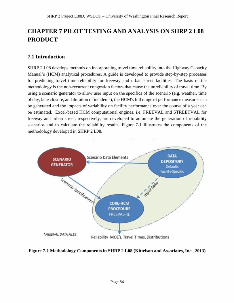
SHRP 2 Project L38D, WSDOT – University of Washington Final Research Report
Page 84
CHAPTER 7 PILOT TESTING AND ANALYSIS ON SHRP 2 L08
PRODUCT
7.1 Introduction
SHRP 2 L08 develops methods on incorporating travel time reliability into the Highway Capacity
Manual’s (HCM) analytical procedures. A guide is developed to provide step-by-step processes
for predicting travel time reliability for freeway and urban street facilities. The basis of the
methodology is the non-recurrent congestion factors that cause the unreliability of travel time. By
using a scenario generator to allow user input on the specifics of the scenario (e.g. weather, time
of day, lane closure, and duration of incidents), the HCM's full range of performance measures can
be generated and the impacts of variability on facility performance over the course of a year can
be estimated. Excel-based HCM computational engines, i.e. FREEVAL and STREETVAL for
freeway and urban street, respectively, are developed to automate the generation of reliability
scenarios and to calculate the reliability results. Figure 7-1 illustrates the components of the
methodology developed in SHRP 2 L08.
Figure 7-1 Methodology Components in SHRP 2 L08 (Kittelson and Associates, Inc., 2013)

SHRP 2 Project L38D, WSDOT – University of Washington Final Research Report
Page 85
7.2 Tool Operability
Both of the L08 reliability tools, STREETVAL and FREEVAL, were tested on Windows 7 and
Windows 8 operating systems as well as a Mac computer running on the most current operating
system, OS X 10.9. The specifications of the computers tested: operating system, system type,
and version of MS office installed, are listed in Table 7-1.
Table 7-1 Specifications of Computers Used in Installation Tests
Operating system Windows 8 Windows 7 Windows 7 OS X 10.9
System type 64-bit 32-bit 64-bit N/A
MS Office version MS Office 2010 MS Office 2010 MS Office
2010
Office 2011
for Mac
Both STREETVAL and FREEVAL ran successfully on Windows 7 operating system for both 32
and 64 bit system types. In attempting to run STREETVAL on Windows 8, the program gave the
following error message shown in Figure 7-2. FREEVAL on the other hand ran on Windows 8
with no problems.
Figure 7-2 Compilation Error Message for Windows 8 Test for STREETVAL

SHRP 2 Project L38D, WSDOT – University of Washington Final Research Report
Page 86
Neither STREETVAL nor FREEVAL was able to run on the Mac computer. When attempting to
run FREEVAL, the interface was responsive, enabling the user to enter the name and general
project information for Step 1, however, when progressing to Step 2, the program would crash.
The results of running STREETVAL were equally disappointing; the USCE macro buttons were
unresponsive to the user’s actions. The research team believes these errors are due to compatibility
issues between the Macintosh operating system, which is Unix based, and the Windows operating
system that software was created with. Given that the vast majority of computers used today are
Windows based, this incompatibility is not a major concern.
7.3 FREEVAL Introduction and Interface
Learning to use the FREEVAL tool is challenging due to the complexity of the tool itself and the
lack of clear instruction on how help information can be obtained. Although a user manual on
FREEVAL exists, the user manual requires knowledge that borrows from several other chapters
of the HCM which may not be available when using the tool.
Use of the tool itself can be broken down into five steps that a user must follow in order to conduct
a reliability assessment of a freeway section.
Step 1: Enter project summary Info
Step 2: Create SEED file
Step 3: Scenario Management
Step 4: Create FREEVAL Input file
Step 5: Generate Scenarios and Results
Step 1 is straightforward; the user enters their name and gives a brief summary of the project for
informational purposes.
In Step 2, the user must enter in the study period, start and end times of the reliability reporting
period, the demand seed day, the number of HCM segments, terrain type, and whether there is
ramp meter control in the study section. It should be noted that when specifying the number of
HCM segments, the user must select 3 or more to make the tool work. If the user selects 2 segments
(as shown in Figure 7-3) the program will seem fine and then once you get to the last step it will
give you an error and the user will have to start all over again. Also, if the user forgets to specify
the ramp meter control (as shown in Figure 7-4), the program does not warn the user that something
is wrong until the last step. Fixing these issues would make this tool much more user friendly.
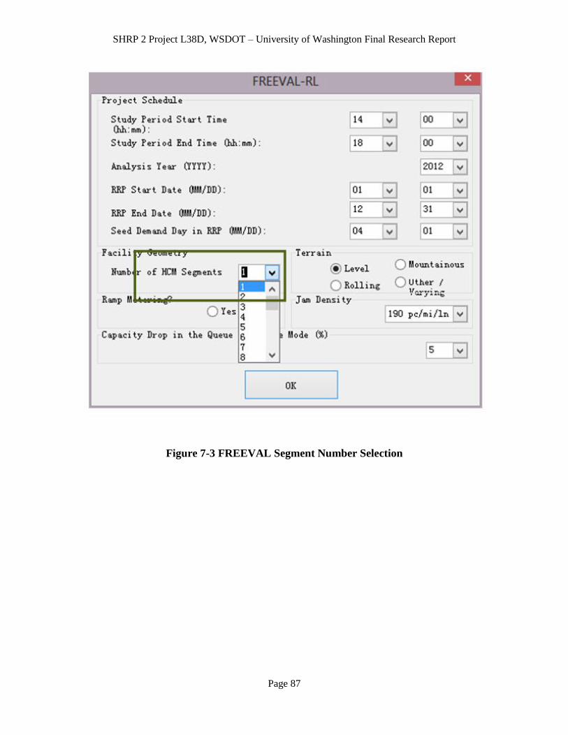
SHRP 2 Project L38D, WSDOT – University of Washington Final Research Report
Page 87
Figure 7-3 FREEVAL Segment Number Selection
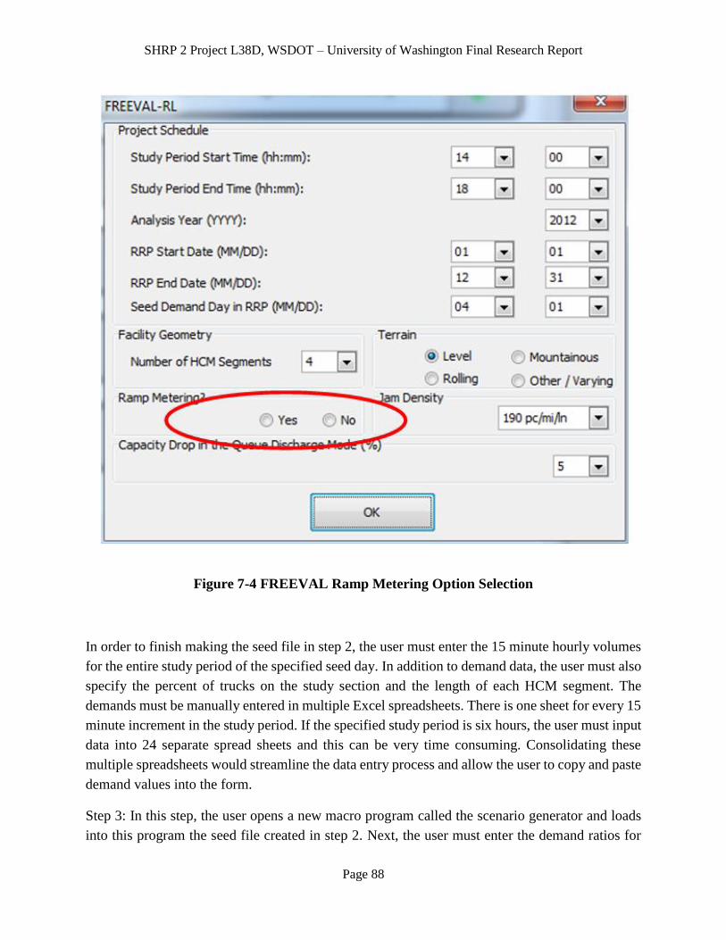
SHRP 2 Project L38D, WSDOT – University of Washington Final Research Report
Page 88
Figure 7-4 FREEVAL Ramp Metering Option Selection
In order to finish making the seed file in step 2, the user must enter the 15 minute hourly volumes
for the entire study period of the specified seed day. In addition to demand data, the user must also
specify the percent of trucks on the study section and the length of each HCM segment. The
demands must be manually entered in multiple Excel spreadsheets. There is one sheet for every 15
minute increment in the study period. If the specified study period is six hours, the user must input
data into 24 separate spread sheets and this can be very time consuming. Consolidating these
multiple spreadsheets would streamline the data entry process and allow the user to copy and paste
demand values into the form.
Step 3: In this step, the user opens a new macro program called the scenario generator and loads
into this program the seed file created in step 2. Next, the user must enter the demand ratios for
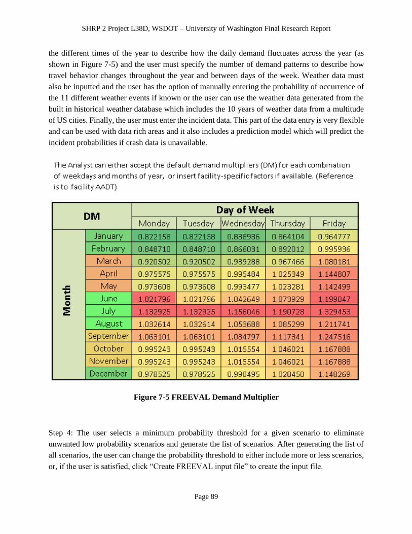
SHRP 2 Project L38D, WSDOT – University of Washington Final Research Report
Page 89
the different times of the year to describe how the daily demand fluctuates across the year (as
shown in Figure 7-5) and the user must specify the number of demand patterns to describe how
travel behavior changes throughout the year and between days of the week. Weather data must
also be inputted and the user has the option of manually entering the probability of occurrence of
the 11 different weather events if known or the user can use the weather data generated from the
built in historical weather database which includes the 10 years of weather data from a multitude
of US cities. Finally, the user must enter the incident data. This part of the data entry is very flexible
and can be used with data rich areas and it also includes a prediction model which will predict the
incident probabilities if crash data is unavailable.
Figure 7-5 FREEVAL Demand Multiplier
Step 4: The user selects a minimum probability threshold for a given scenario to eliminate
unwanted low probability scenarios and generate the list of scenarios. After generating the list of
all scenarios, the user can change the probability threshold to either include more or less scenarios,
or, if the user is satisfied, click “Create FREEVAL input file” to create the input file.

SHRP 2 Project L38D, WSDOT – University of Washington Final Research Report
Page 90
Step 5: The final step in the program involves the user loading the input file created in step 4 back
into the original FREEVAL macro and evaluating the scenarios by clicking “Click generate
scenarios”. This part of the program takes the longest to complete and each scenario in the input
file may take 20-60 seconds to be evaluated.
The primary issues identified with tool use were those addressed in step 2; Warning messages
displayed by the program would alert the users of their mistakes for them to fix. Also, consolidating
the demand input sheets would definitely streamline the data entry process of this program which
can easily take several hours depending on the length of study period and number of HCM
segments.
One issue not addressed in any of the literature regarding FREEVAL is how long of a study section
is good for a particular reliability test. It would seem intuitive that for urban areas with more access
ramps, longer study sections would be preferred, and for more rural areas, a shorter study section
might suffice. More guidance on selecting the appropriate study period would be helpful. In
addition, the software does not address causes of congestion that may occur outside of the study
section; a weaving section located upstream of the test site might be a source of recurring
congestion and will be ignored in an analysis. Because of this, the results of the reliability test may
be skewed.
7.4 Performance Test for FREEVAL
Tests were completed to determine the accuracy of the FREEVAL reliability software by
comparing the outputted travel time reliability from the software to the actual travel time reliability
computed from historical dual-loop detector data. The tests were conducted for two separate study
locations in Seattle, WA and are circled in the map (Figure 7-6). The green circle shows the I-5
study site, which goes from the Northgate Mall to Shoreline (roughly 3 miles long), and the red
circle indicates the I-405 study site (roughly 2 miles long) , which is located just outside the city
in a less urban environment.
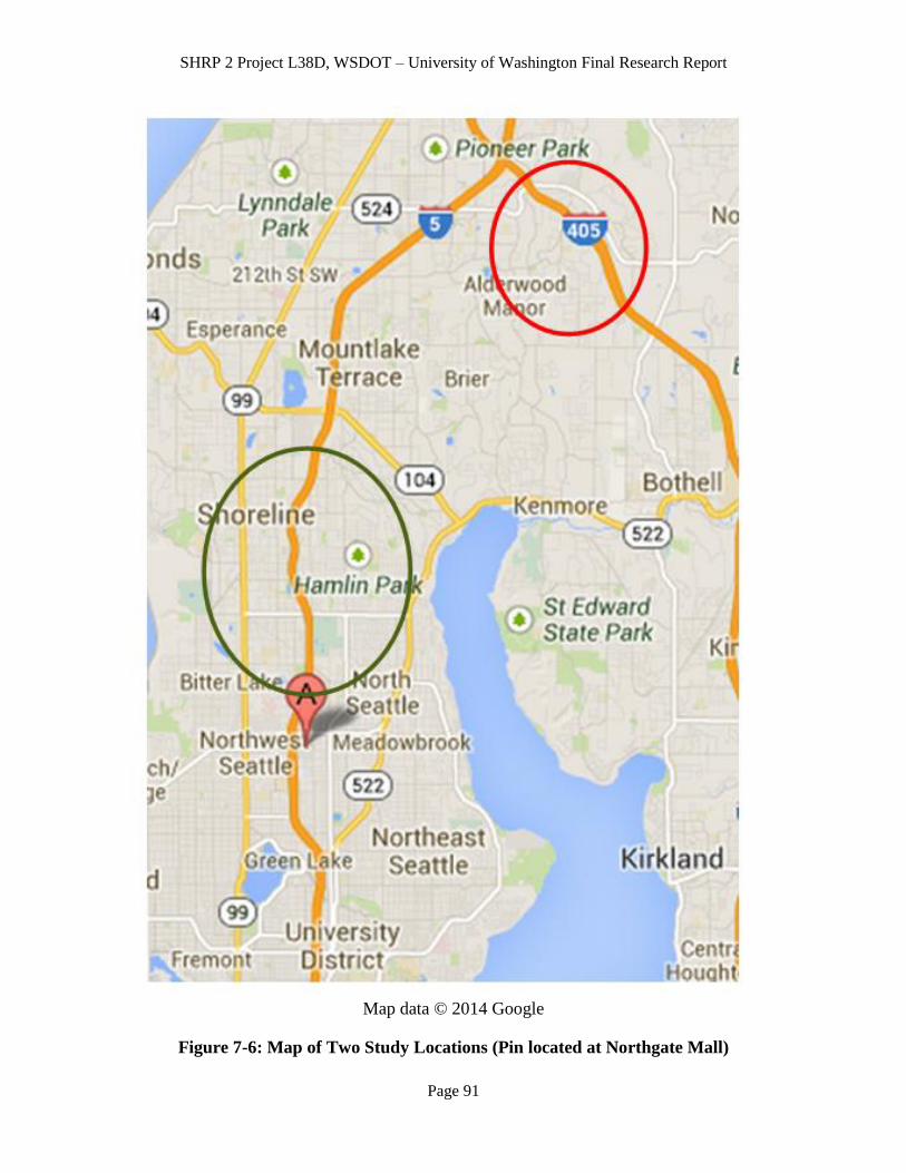
SHRP 2 Project L38D, WSDOT – University of Washington Final Research Report
Page 91
Map data © 2014 Google
Figure 7-6: Map of Two Study Locations (Pin located at Northgate Mall)
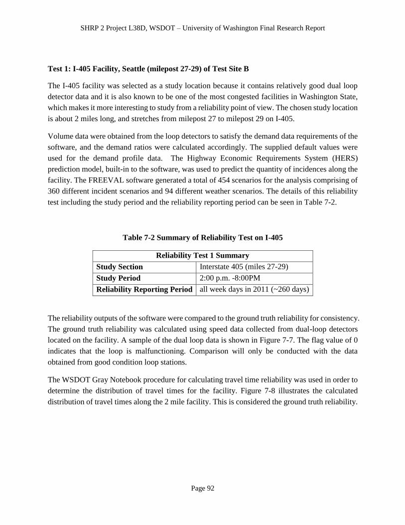
SHRP 2 Project L38D, WSDOT – University of Washington Final Research Report
Page 92
Test 1: I-405 Facility, Seattle (milepost 27-29) of Test Site B
The I-405 facility was selected as a study location because it contains relatively good dual loop
detector data and it is also known to be one of the most congested facilities in Washington State,
which makes it more interesting to study from a reliability point of view. The chosen study location
is about 2 miles long, and stretches from milepost 27 to milepost 29 on I-405.
Volume data were obtained from the loop detectors to satisfy the demand data requirements of the
software, and the demand ratios were calculated accordingly. The supplied default values were
used for the demand profile data. The Highway Economic Requirements System (HERS)
prediction model, built-in to the software, was used to predict the quantity of incidences along the
facility. The FREEVAL software generated a total of 454 scenarios for the analysis comprising of
360 different incident scenarios and 94 different weather scenarios. The details of this reliability
test including the study period and the reliability reporting period can be seen in Table 7-2.
Table 7-2 Summary of Reliability Test on I-405
Reliability Test 1 Summary
Study Section Interstate 405 (miles 27-29)
Study Period 2:00 p.m. -8:00PM
Reliability Reporting Period all week days in 2011 (~260 days)
The reliability outputs of the software were compared to the ground truth reliability for consistency.
The ground truth reliability was calculated using speed data collected from dual-loop detectors
located on the facility. A sample of the dual loop data is shown in Figure 7-7. The flag value of 0
indicates that the loop is malfunctioning. Comparison will only be conducted with the data
obtained from good condition loop stations.
The WSDOT Gray Notebook procedure for calculating travel time reliability was used in order to
determine the distribution of travel times for the facility. Figure 7-8 illustrates the calculated
distribution of travel times along the 2 mile facility. This is considered the ground truth reliability.
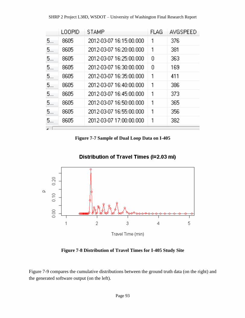
SHRP 2 Project L38D, WSDOT – University of Washington Final Research Report
Page 93
Figure 7-7 Sample of Dual Loop Data on I-405
Figure 7-8 Distribution of Travel Times for I-405 Study Site
Figure 7-9 compares the cumulative distributions between the ground truth data (on the right) and
the generated software output (on the left).

SHRP 2 Project L38D, WSDOT – University of Washington Final Research Report
Page 94
(a) FREEVAL Output (b) Dual Loop Data
Figure 7-9 Comparison of Cumulative Distributions for TTI on I-405
According to Table 7-3, it is evident that the FREEVAL estimate of reliability tends to be overly
optimistic; its TTI values are almost all smaller than the ground truth. The semi standard deviation
(the standard deviation taken about the free flow travel time instead of the mean) estimated by
FREEVAL is more or less the same with the ground truth value while the 80th percentile TTI and
95th percentile TTI values for the ground truth data are larger than FREEVAL outputs.
Table 7-3 Performance Measure comparison
Performance Measure FREEVAL Ground Truth
Mean TTI 1.11 1.16
50th Percentile TTI 1.08 1.03
80th Percentile TTI 1.14 1.30
95th Percentile TTI 1.25 1.55
Semi Standard Dev. 0.45min 0.46min
Test 2: I-5 Facility, Seattle (milepost 173-176) on Test Site A
The second study facility is I-5 near the Northgate Mall. This site is chosen because it is a well-
known congested section of roadway and it has a high density of access ramps that makes it
different from the I-405 test site, which had no access ramps. The on-ramps and off-ramps for the
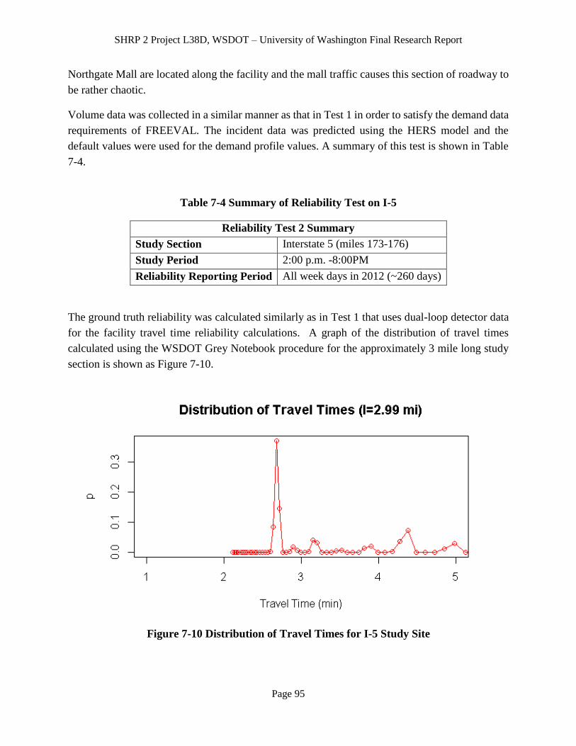
SHRP 2 Project L38D, WSDOT – University of Washington Final Research Report
Page 95
Northgate Mall are located along the facility and the mall traffic causes this section of roadway to
be rather chaotic.
Volume data was collected in a similar manner as that in Test 1 in order to satisfy the demand data
requirements of FREEVAL. The incident data was predicted using the HERS model and the
default values were used for the demand profile values. A summary of this test is shown in Table
7-4.
Table 7-4 Summary of Reliability Test on I-5
Reliability Test 2 Summary
Study Section Interstate 5 (miles 173-176)
Study Period 2:00 p.m. -8:00PM
Reliability Reporting Period All week days in 2012 (~260 days)
The ground truth reliability was calculated similarly as in Test 1 that uses dual-loop detector data
for the facility travel time reliability calculations. A graph of the distribution of travel times
calculated using the WSDOT Grey Notebook procedure for the approximately 3 mile long study
section is shown as Figure 7-10.
Figure 7-10 Distribution of Travel Times for I-5 Study Site
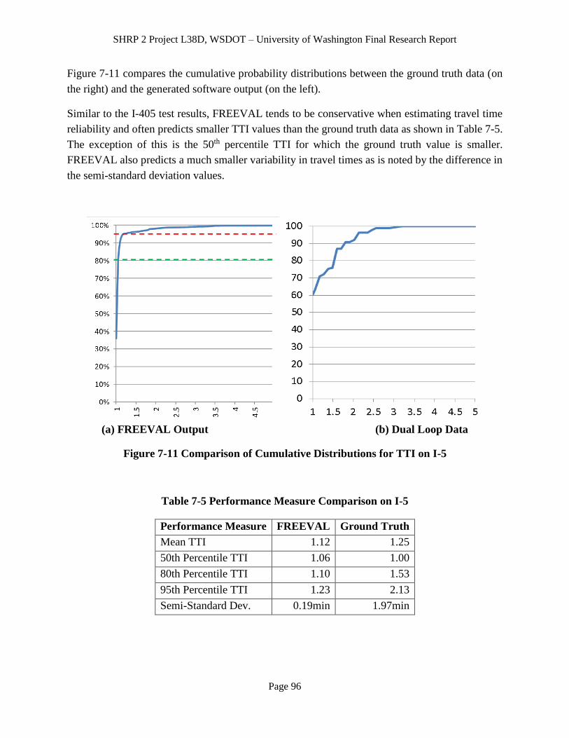
SHRP 2 Project L38D, WSDOT – University of Washington Final Research Report
Page 96
Figure 7-11 compares the cumulative probability distributions between the ground truth data (on
the right) and the generated software output (on the left).
Similar to the I-405 test results, FREEVAL tends to be conservative when estimating travel time
reliability and often predicts smaller TTI values than the ground truth data as shown in Table 7-5.
The exception of this is the 50th percentile TTI for which the ground truth value is smaller.
FREEVAL also predicts a much smaller variability in travel times as is noted by the difference in
the semi-standard deviation values.
(a) FREEVAL Output (b) Dual Loop Data
Figure 7-11 Comparison of Cumulative Distributions for TTI on I-5
Table 7-5 Performance Measure Comparison on I-5
Performance Measure FREEVAL Ground Truth
Mean TTI 1.12 1.25
50th Percentile TTI 1.06 1.00
80th Percentile TTI 1.10 1.53
95th Percentile TTI 1.23 2.13
Semi-Standard Dev. 0.19min 1.97min
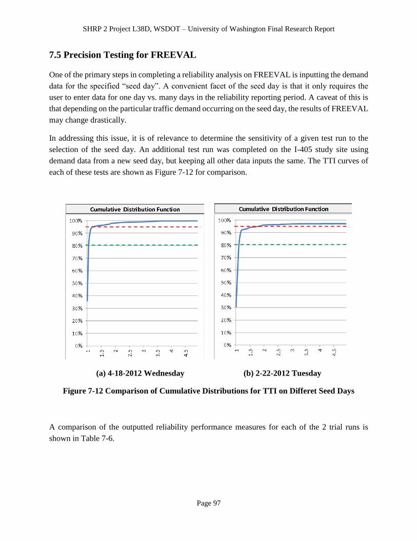
SHRP 2 Project L38D, WSDOT – University of Washington Final Research Report
Page 97
7.5 Precision Testing for FREEVAL
One of the primary steps in completing a reliability analysis on FREEVAL is inputting the demand
data for the specified “seed day”. A convenient facet of the seed day is that it only requires the
user to enter data for one day vs. many days in the reliability reporting period. A caveat of this is
that depending on the particular traffic demand occurring on the seed day, the results of FREEVAL
may change drastically.
In addressing this issue, it is of relevance to determine the sensitivity of a given test run to the
selection of the seed day. An additional test run was completed on the I-405 study site using
demand data from a new seed day, but keeping all other data inputs the same. The TTI curves of
each of these tests are shown as Figure 7-12 for comparison.
(a) 4-18-2012 Wednesday (b) 2-22-2012 Tuesday
Figure 7-12 Comparison of Cumulative Distributions for TTI on Differet Seed Days
A comparison of the outputted reliability performance measures for each of the 2 trial runs is
shown in Table 7-6.
SHRP 2 Project L38D, WSDOT – University of Washington Final Research Report
Page 98
Table 7-6 Test Result Comparison between Seed Days
Performance Measures
Run 1
4-18-2012 Wednesday
Run 2
2-22-2012 Tuesday
Mean TTI 1.11 1.12
50th Percentile TTI 1.08 1.08
80th percentile TTI 1.14 1.15
95th Percentile TTI (PTI) 1.25 1.27
Misery Index 1.90 1.96
Semi-Standard Deviation 0.45 0.45
Reliability Rating 95.75% 90.30%
Percent VMT at TTI > 2 1.04% 1.27%
According to Figure 7-12 and Table 7-6, the difference on MOEs between the two trial runs is not
large nonetheless the selection of the seed day can affect the results. Also, it is not sufficient to
only complete one trial run. Doing so may grossly misrepresent the actual reliability of a facility.
Multiple runs must be completed and the results must be analyzed statistically in order to be
confident in the results of a FREEVAL reliability test.
The only instructions given to the user for selecting the seed day are that the seed day should be
included in the reliability reporting period, and that it should be a day in which no special events,
such as big sports games, are occurring. There is no indication that multiple runs should be
completed using the demand data from several different seed days in order for a test to be reliable.
This should be clearly addressed in the L08 documents.
7.6 Test Conclusions for FREEVAL
In summary, although it is impossible to evaluate the accuracy of FREEVAL based on the results
of two tests, it is fair to say that the reliability estimates of the software seem reasonable compared
to the ground truth reliability determined from the dual-loop detector data. Overall, FREEVAL
tends to be over-optimistic in its estimates and produced consistently smaller TTI values and
smaller semi-standard deviations.
7.7 STREETVAL Introduction and Interface
The Urban Streets Reliability Engine tool (STREETVAL) was developed for the purpose of
assessing the long term travel time reliability along a signalized arterial. In order to carry out its

SHRP 2 Project L38D, WSDOT – University of Washington Final Research Report
Page 99
procedure for predicting long term travel time reliability, two specific methodologies are
implemented and are referred in the literature as the reliability methodology, and the HCM
methodology. These two methodologies are described briefly below, however, a more detailed
description can be found in the in the STREETVAL user guide.
Reliability Methodology: The reliability methodology uses a random statistical procedure, guided
by an inputted base data set, to simulate the traffic demand, weather and incident conditions over
each of many small time periods (analysis periods) within the study period and for each day in the
reliability reporting period. This process is also referred in the literature as the scenario generation
procedure.
HCM Methodology: This methodology predicts the travel times on the specified corridor, given
the predetermined traffic, weather and incident conditions from the reliability methodology, for
each of the analysis periods within the study period and for each day in the reliability reporting
period. Note: this methodology also includes procedures for estimating travel times during work
zones and special events
The flow chart shown in Figure 7-13 illustrates how these two methodologies interact in order to
perform a reliability assessment.
To further elaborate on the STREETVAL reliability procedure from a software analyst perspective,
use of the tool has been broken down into five main actions as follows: action 1: selection of
project purpose, location, and scope; action 2: HCM input data file creation; action 3: scenario
generation; action 4: scenario evaluation; action 5: result interpretation.
Step 1:
Prior to beginning an analysis, it is recommended that the user has a clear idea of what is to be
gained in doing such an analysis, namely what is the project purpose. There are many possible
motivations for using STREETVAL, which are discussed in the literature. These include:
Evaluating potential improvements (i.e., signal retiming, infrastructure improvements, etc.);
Determining key sources of travel time unreliability;
Quantifying problems.

SHRP 2 Project L38D, WSDOT – University of Washington Final Research Report
Page 100
Figure 7-13 STREETVAL methodology flowchart
A manageable project scope must be selected which consists of both the project study site and
temporal scope. In selecting the study location the user is constrained on the length of roadway
that can be evaluated. The study location must contain no more than 9 signalized intersections
(eight analysis segments). For the temporal scope, the user must specify three parameters: analysis
period, study period, and reliability reporting period. These parameters are briefly defined below:
Study Period:
It is recommended that the study period for a given project be a maximum of 6 hours, and no less
than 1 full hour. The study period should be selected such that the first analysis period within the
study period is uncongested.
Analysis Period:
The analysis period essentially defines the resolution analysis that will be performed by the
software. This period can range anywhere from 15 minutes to 1 hour. It is however recommended
for operational analyzes, that a 15 minute period be selected. The selection of a longer period may

SHRP 2 Project L38D, WSDOT – University of Washington Final Research Report
Page 101
cause incident and weather events lasting only a short period of time (such as a brief hard hailstorm)
to be ignored.
Reliability Reporting Period:
The reliability reporting period (RRP) should be relatively long (not less than 200 days). The
analyst may choose which days of the week to be included in the RRP (for example exclude
weekends, or all Mondays, etc.).
Step 2: HCM Input data file creation
This step requires the user to input the required input data into the Urban Streets Computational
Engine program, which is an excel macro, in order to create an input file of type .txt which can be
read by the Urban Streets Reliability Engine. (A screen shot of this tool is shown in Figure 7-14.)
The necessary input data required includes:
1) demand data for each intersection and access point located;
2) study section roadway geometric data;
3) signal timing data for each intersection.
These sources of data will be further discussed in the following section. The USCE divides the
study location into analysis segments, bounded on either end by a signalized intersection and
allocates an excel sheet for each analysis segment as well as one sheet for the first segment
intersection (as shown in Figure 7-15). The three previously listed types of data must be entered
for each individual segment along the study section.

SHRP 2 Project L38D, WSDOT – University of Washington Final Research Report
Page 102
Figure 7-14 Urban Streets Computation Engine (USCE).
Figure 7-15 STREETVAL Segment Schematic
After entering all the necessary data, the user writes the data to a file which is saved to a user-
specified directory. He/she is then prepared for the next step.
Step 3: Scenario Generation

SHRP 2 Project L38D, WSDOT – University of Washington Final Research Report
Page 103
The scenario generation step is carried out using the Urban Streets Reliability Engine (USRE),
which is also an excel macro program.
Figure 7-16 USRE 2010 HCM
The user must first upload the HCM input file created in Step 2, specify the time and date of the
seed demand data specified in the input file (1 hour of collected volume data), as well as enter the
three temporal scope variables for the project. These values are entered in the “Set up” layer of the
tool. In addition to these values, crash data, peak hour factors for traffic (if using 15 analysis period
and wish to randomize demand within 15 minute periods), and work zones and special event input
files if they are deemed necessary and relevant. As previously mentioned, the scenario generation
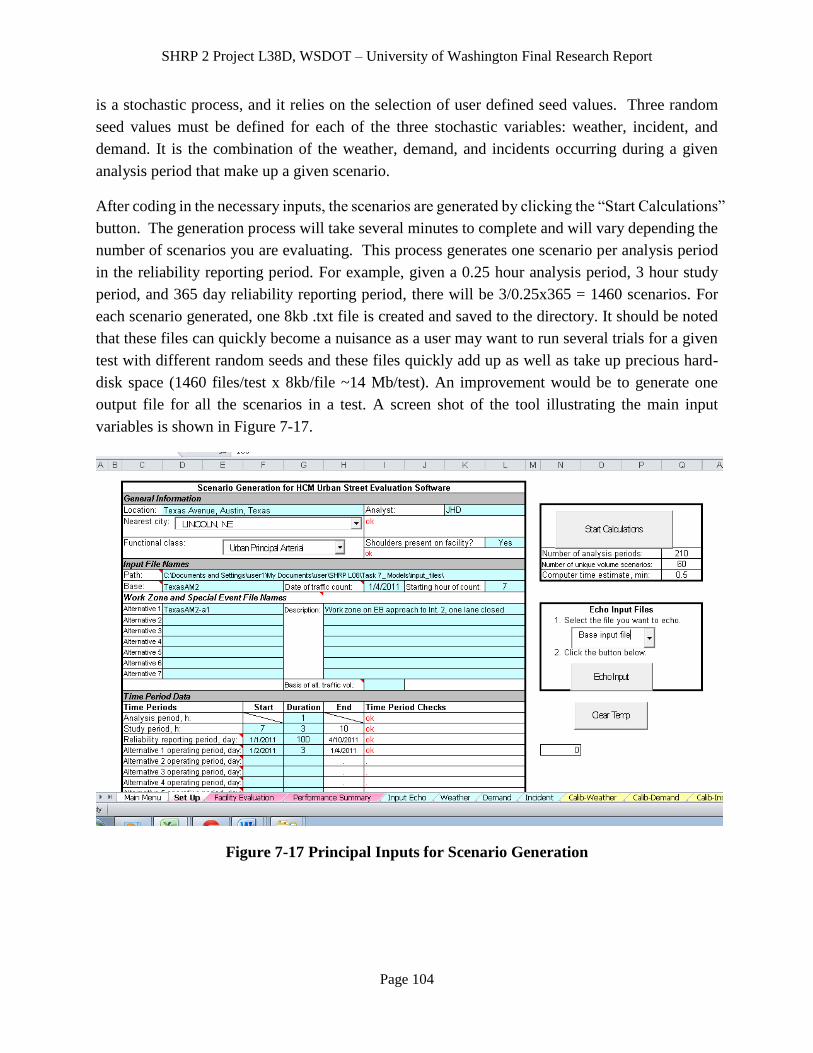
SHRP 2 Project L38D, WSDOT – University of Washington Final Research Report
Page 104
is a stochastic process, and it relies on the selection of user defined seed values. Three random
seed values must be defined for each of the three stochastic variables: weather, incident, and
demand. It is the combination of the weather, demand, and incidents occurring during a given
analysis period that make up a given scenario.
After coding in the necessary inputs, the scenarios are generated by clicking the “Start Calculations”
button. The generation process will take several minutes to complete and will vary depending the
number of scenarios you are evaluating. This process generates one scenario per analysis period
in the reliability reporting period. For example, given a 0.25 hour analysis period, 3 hour study
period, and 365 day reliability reporting period, there will be 3/0.25x365 = 1460 scenarios. For
each scenario generated, one 8kb .txt file is created and saved to the directory. It should be noted
that these files can quickly become a nuisance as a user may want to run several trials for a given
test with different random seeds and these files quickly add up as well as take up precious hard-
disk space (1460 files/test x 8kb/file ~14 Mb/test). An improvement would be to generate one
output file for all the scenarios in a test. A screen shot of the tool illustrating the main input
variables is shown in Figure 7-17.
Figure 7-17 Principal Inputs for Scenario Generation

SHRP 2 Project L38D, WSDOT – University of Washington Final Research Report
Page 105
Figure 7-18 Random seed numbers and PHF
Step 4: Scenario Evaluation
This is the start of the HCM methodology and it consists evaluating the scenarios that were
previously generated. In order to evaluate each scenario, the scenario engine is utilized. The
scenario engine, which has not yet been mentioned in this report, is a .zip file that contains the
operational procedures based on previously conducted research to estimate travel time
performance measures for a given scenario. This step is the second most computationally intensive
step after scenario generation and typically takes 3-6 minutes depending on the number of
scenarios being evaluated.
An “evaluation interval” parameter gives the user the choice to either evaluate all the generated
scenarios or a subset of them. This can greatly reduce the required computation time however at
the cost of an overall smaller sample size.
Figure 7-19 shows a screen show of the scenario evaluation sheet of USRE. Two sources of data
are entered in this sheet: they are the “Engine Path”, which is the location of the scenario
generator .zip file, and the evaluation interval that has just been discussed.
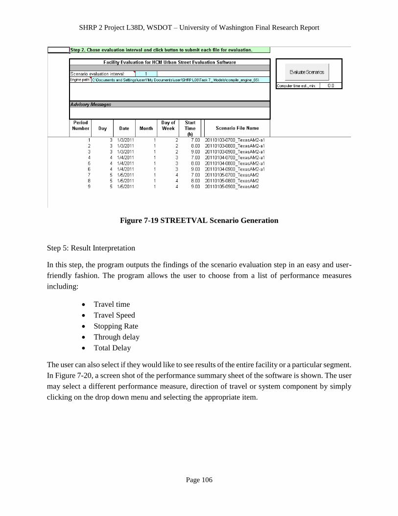
SHRP 2 Project L38D, WSDOT – University of Washington Final Research Report
Page 106
Figure 7-19 STREETVAL Scenario Generation
Step 5: Result Interpretation
In this step, the program outputs the findings of the scenario evaluation step in an easy and user-
friendly fashion. The program allows the user to choose from a list of performance measures
including:
Travel time
Travel Speed
Stopping Rate
Through delay
Total Delay
The user can also select if they would like to see results of the entire facility or a particular segment.
In Figure 7-20, a screen shot of the performance summary sheet of the software is shown. The user
may select a different performance measure, direction of travel or system component by simply
clicking on the drop down menu and selecting the appropriate item.
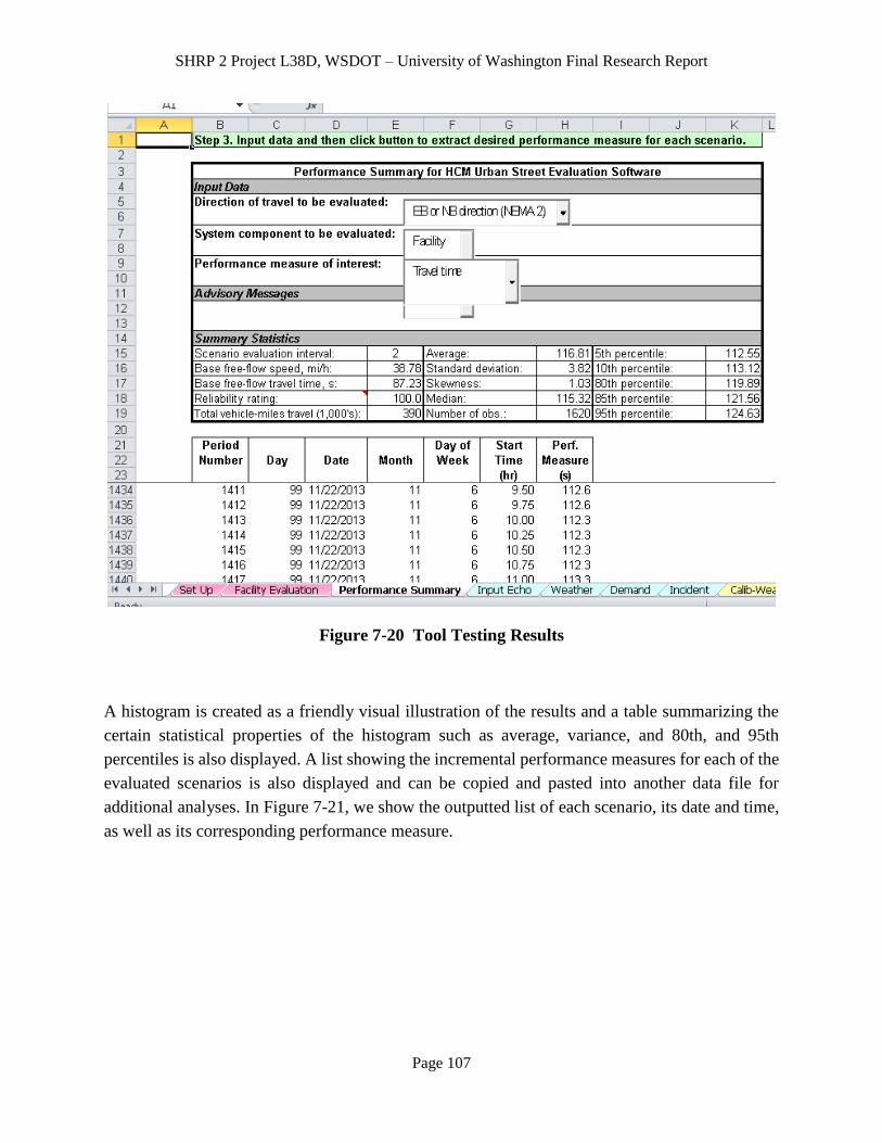
SHRP 2 Project L38D, WSDOT – University of Washington Final Research Report
Page 107
Figure 7-20 Tool Testing Results
A histogram is created as a friendly visual illustration of the results and a table summarizing the
certain statistical properties of the histogram such as average, variance, and 80th, and 95th
percentiles is also displayed. A list showing the incremental performance measures for each of the
evaluated scenarios is also displayed and can be copied and pasted into another data file for
additional analyses. In Figure 7-21, we show the outputted list of each scenario, its date and time,
as well as its corresponding performance measure.
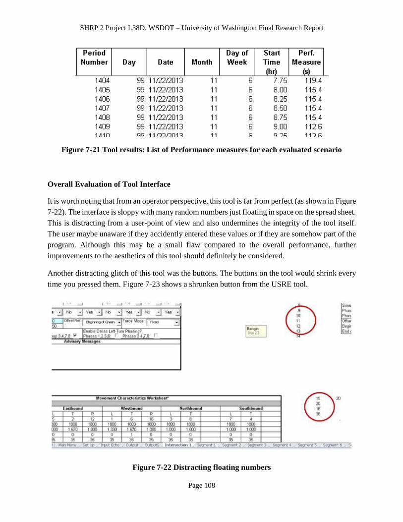
SHRP 2 Project L38D, WSDOT – University of Washington Final Research Report
Page 108
Figure 7-21 Tool results: List of Performance measures for each evaluated scenario
Overall Evaluation of Tool Interface
It is worth noting that from an operator perspective, this tool is far from perfect (as shown in Figure
7-22). The interface is sloppy with many random numbers just floating in space on the spread sheet.
This is distracting from a user-point of view and also undermines the integrity of the tool itself.
The user maybe unaware if they accidently entered these values or if they are somehow part of the
program. Although this may be a small flaw compared to the overall performance, further
improvements to the aesthetics of this tool should definitely be considered.
Another distracting glitch of this tool was the buttons. The buttons on the tool would shrink every
time you pressed them. Figure 7-23 shows a shrunken button from the USRE tool.
Figure 7-22 Distracting floating numbers
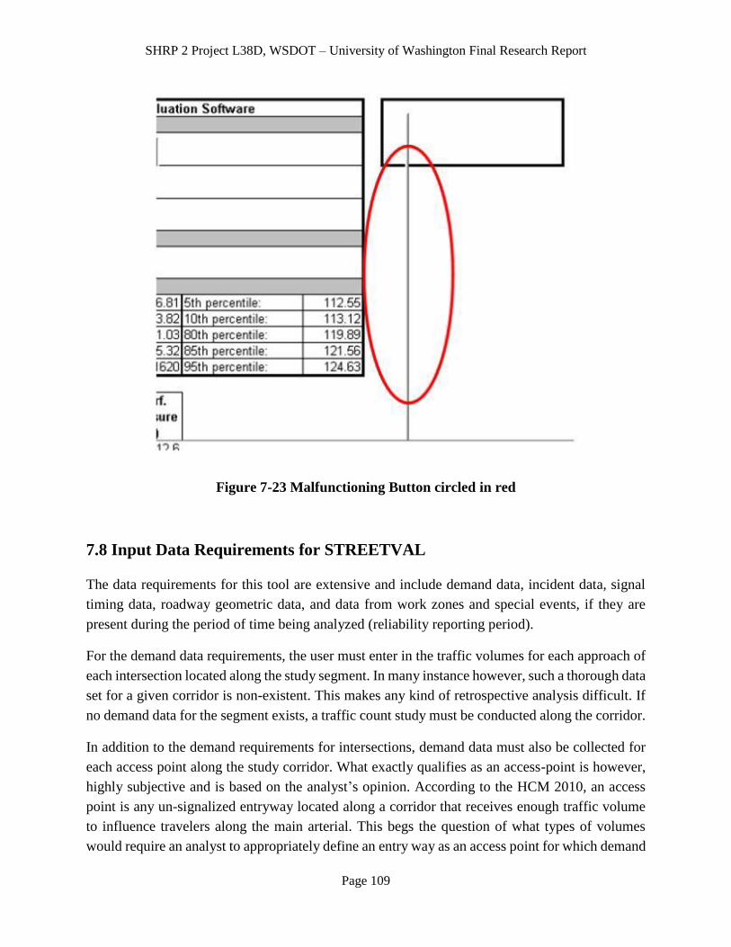
SHRP 2 Project L38D, WSDOT – University of Washington Final Research Report
Page 109
Figure 7-23 Malfunctioning Button circled in red
7.8 Input Data Requirements for STREETVAL
The data requirements for this tool are extensive and include demand data, incident data, signal
timing data, roadway geometric data, and data from work zones and special events, if they are
present during the period of time being analyzed (reliability reporting period).
For the demand data requirements, the user must enter in the traffic volumes for each approach of
each intersection located along the study segment. In many instance however, such a thorough data
set for a given corridor is non-existent. This makes any kind of retrospective analysis difficult. If
no demand data for the segment exists, a traffic count study must be conducted along the corridor.
In addition to the demand requirements for intersections, demand data must also be collected for
each access point along the study corridor. What exactly qualifies as an access-point is however,
highly subjective and is based on the analyst’s opinion. According to the HCM 2010, an access
point is any un-signalized entryway located along a corridor that receives enough traffic volume
to influence travelers along the main arterial. This begs the question of what types of volumes
would require an analyst to appropriately define an entry way as an access point for which demand

SHRP 2 Project L38D, WSDOT – University of Washington Final Research Report
Page 110
data will need to be collected. If multiple smaller access points are located along the corridor, the
tool recommends combining these access points into one single access point that is located at the
average distance of each smaller access point from the upstream intersection and that receives the
combined volumes of each of the smaller access. In most cases, where access point demand data
is unavailable, a traffic count study is required and this process is labor intensive and costly to an
agency.
One improvement to the tool might be to provide a method to estimate access point data along an
urban arterial based on a number of built-environmental factors that are likely to be of influence,
such as: land type, population density, parking lot size, time of day, and distance from Central
Business District (CBD).
For the incident data requirements, crash segment frequencies must be specified for each
intersection and each segment. Crashes are considered to be intersection-related if they occur
within the bounds of the intersection itself, if they occur as a result of a queue formed from the
intersection bottleneck, or if they are caused by a traffic signal controller malfunction. If an
incident cannot be classified as intersection-related, it is classified as segment-related. In most
cases, the cause of the incident can be used to deduce the type of crash (intersection-related or
segment-related).
The user manual suggests two methods to calculate the crash segment frequencies (expected
number of crashes at given location (crashes/year)). The first method requires the user to have
access to at least three years’ worth of crash data. This data may then be used to calculate the crash
frequencies, based on the average crash frequency during the three years of collected data. The
second method involves using the 2010 Highway Safety Manual (HSM) methodology, which is
described in Chapter 12.
Signal timing data must be acquired from each of the traffic signals located along the study corridor
and is a crucial component in the estimation of segment level travel times. STREETVAL software
is capable of accommodating both pre-timed control, and actuated/semi-actuated control operating
under coordinated conditions, where several adjacent intersections are in-sync and timed to a
master controller or isolated control, where adjacent intersections have no communication with
one another and act as independent entities.
In addition to the previously described data types, STREETVAL also requires weather data for the
given study location including: average monthly rainfall, days with rainfall greater than 0.01 inches,
average monthly snowfall, and average monthly temperatures. The STREETVAL tool contains to
a large databank with ten years of weather data for many prominent US cities and towns. This
eliminates the need to acquire adequate weather data and streamlines the overall reliability testing
procedure.
SHRP 2 Project L38D, WSDOT – University of Washington Final Research Report
Page 111
Prior to collecting and gathering this data (signal timing, demand, crash, and weather data) from
multiple various sources, the user must first determine when is the best time to collect or gather
this data. The analyst must be certain that the demand data (collected for the 1 hour period during
the study period) is collected at an appropriate time. Before this can be done, the analyst must
appropriately define the temporal scope of the project. In STREETVAL, the temporal scope is
defined equivalently as it was for FREEVAL. The user must choose the study period, analysis
period and reliability reporting period. These three parameters were defined previously.
7.9 Performance Test for STREETVAL
Test Site Location: In order to test the accuracy of this tool, a test was conducted on an urban
arterial using real traffic data. The test location selected is a roughly 1 mile stretch of SR 522, an
urban arterial located in Kenmore, WA, just outside of Seattle. This site, shown in the map (Figure
7-24), provides traveler’s access to both Interstate 5 and Interstate 405 and serves as a major route
around Lake Washington for those commuting into the city from the neighboring suburbs. This
particular site location was selected both because it acts as a major daily commute route for
intercity travel and because of the abundance of sensor infrastructure that is currently installed
along it, including automated license plate reader (ALPR) cameras, which collect very accurate
travel time data. The travel time data gathered from these cameras served as a ground truth base
from which to assess the accuracy of STREETVAL.

SHRP 2 Project L38D, WSDOT – University of Washington Final Research Report
Page 112
Map data © 2014 Google
Figure 7-24 Study site location along SR 522, Kenmore, WA.
As mentioned previously, testing the reliability of a corridor using the STREETVAL tool requires
that a large amount of data first be gathered. Even though the research team currently has access
to all of the loop detector data and live video feeds from several gantry-mounted video cameras
along the study site, not to mention, an array travel time data obtained from Bluetooth sensors and
automated-license plate reader cameras, the demand data requirements of the tool could not be
satisfied using data collected from the existing sensors. The reason for this was that the tool
requires demand data for each movement of each intersection and the rich sensor infrastructure
installed along the study site only gave us complete demand data for the main SR 522 arterial and
not the side streets. When we became aware of this problem we had one of two choices: 1) try to
find another urban arterial with more complete demand data, or 2) manually collect the missing
demand data for SR 522. After some debate, it was decided that SR 522 would stay as our test
sight and that we would collect the missing data for the other intersections approaches manually.
There were two primary reasons for this decision. The first reason is that we were not able to find
complete demand data for all signalized intersection approaches on an urban arterial. The second

SHRP 2 Project L38D, WSDOT – University of Washington Final Research Report
Page 113
reason is that SR 522 was the only known arterial in Seattle which had accessible ground truth
travel time data.
Volume Data Collection: Due to limited resources for the manual data collection, the originally
proposed study site of roughly 4 miles in length, was shrunk down to a manageable 1 mile section,
stretching along SR 522 from 68th Ave to 83rd Pl (see Figure 7-25).
Map data © 2014 Google
Figure 7-25 Study Site Location
To satisfy the traffic volume data input requirements of the tool, one-hour traffic volumes were
simultaneously captured for all five intersections located along the study site using 7 tripod-
mounted video cameras for 2 one-hour periods. The complexity of the intersections and high rate
of vehicle arrivals made it necessary to capture the volume data with a camera. This camera data
was later viewed at a slower more convenient pace and the traffic volumes for each direction were
obtained. Images captured from each of the 7 tripod-mounted cameras are shown directly in Figure
7-26. These cameras were situated so that all traffic from each individual approach could be
observed.

SHRP 2 Project L38D, WSDOT – University of Washington Final Research Report
Page 114
(a) 68th Ave Camera captured images from video of four-way intersection (EB/WB (upper
figure) and NB/SB (lower figure) approaches)

SHRP 2 Project L38D, WSDOT – University of Washington Final Research Report
Page 115
(b) 73rd Ave Camera captured images of four-way intersection (EB/WB (upper figure) and
NB/SB (lower figure) approaches)
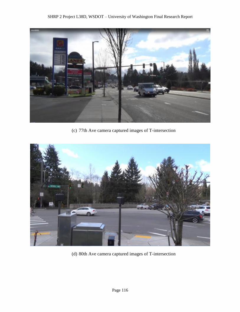
SHRP 2 Project L38D, WSDOT – University of Washington Final Research Report
Page 116
(c) 77th Ave camera captured images of T-intersection
(d) 80th Ave camera captured images of T-intersection

SHRP 2 Project L38D, WSDOT – University of Washington Final Research Report
Page 117
(e) 83rd Pl camera captured image of T-intersection
Figure 7-26 Camera Captured Images of Studied Intersections
To further aid in the traffic counting process, a software program, Traffic Counter (shown in Figure
7-27), was developed by STAR Lab members which allows the user to count traffic on the
computer by pressing the appropriate key for a given direction. The advantage of this software is
that the user can touch type the keys and thereby. And the user does not have to take their eyes off
the video and risk missing a count. This was crucial because traffic is often running at or near the
saturation flow rate at the startup of the green phase, which requires a high level of visual attention
to count.
Volume data was also collected via manual counting at all of the major access points along the
study site. To aid with the data collection, a team of ten volunteers were needed. Each volunteer
was given a particular task: either manually counting cars at an access point, or filming vehicles
passing through an intersection using a tripod-mounted camcorder. In total, approximately 67 man
hours were spent both collecting data at the sight and counting vehicles from the videos that were
recorded This is worth mentioning because any agency that will, in the future, be using this tool,
will want to consider the potential costs of collecting the data to use it. The cost of 67 hours of
labor is not trivial, and that’s not considering the opportunity cost of sending 10 trained engineers
from an agency or consulting firm to count cars.
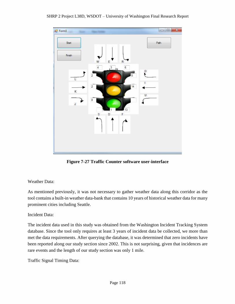
SHRP 2 Project L38D, WSDOT – University of Washington Final Research Report
Page 118
Figure 7-27 Traffic Counter software user-interface
Weather Data:
As mentioned previously, it was not necessary to gather weather data along this corridor as the
tool contains a built-in weather data-bank that contains 10 years of historical weather data for many
prominent cities including Seattle.
Incident Data:
The incident data used in this study was obtained from the Washington Incident Tracking System
database. Since the tool only requires at least 3 years of incident data be collected, we more than
met the data requirements. After querying the database, it was determined that zero incidents have
been reported along our study section since 2002. This is not surprising, given that incidences are
rare events and the length of our study section was only 1 mile.
Traffic Signal Timing Data:
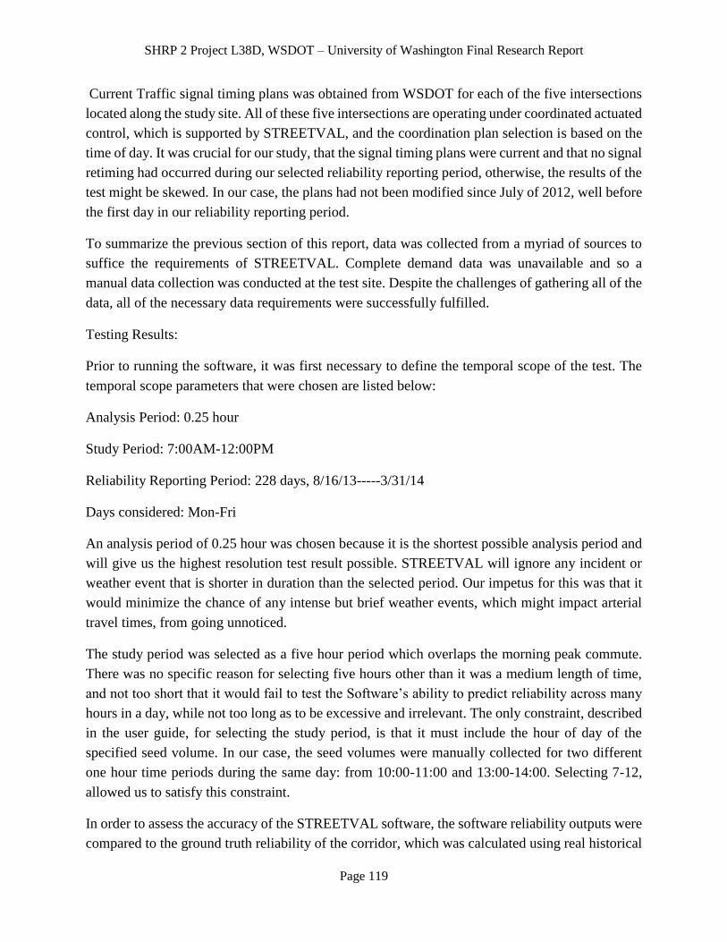
SHRP 2 Project L38D, WSDOT – University of Washington Final Research Report
Page 119
Current Traffic signal timing plans was obtained from WSDOT for each of the five intersections
located along the study site. All of these five intersections are operating under coordinated actuated
control, which is supported by STREETVAL, and the coordination plan selection is based on the
time of day. It was crucial for our study, that the signal timing plans were current and that no signal
retiming had occurred during our selected reliability reporting period, otherwise, the results of the
test might be skewed. In our case, the plans had not been modified since July of 2012, well before
the first day in our reliability reporting period.
To summarize the previous section of this report, data was collected from a myriad of sources to
suffice the requirements of STREETVAL. Complete demand data was unavailable and so a
manual data collection was conducted at the test site. Despite the challenges of gathering all of the
data, all of the necessary data requirements were successfully fulfilled.
Testing Results:
Prior to running the software, it was first necessary to define the temporal scope of the test. The
temporal scope parameters that were chosen are listed below:
Analysis Period: 0.25 hour
Study Period: 7:00AM-12:00PM
Reliability Reporting Period: 228 days, 8/16/13-----3/31/14
Days considered: Mon-Fri
An analysis period of 0.25 hour was chosen because it is the shortest possible analysis period and
will give us the highest resolution test result possible. STREETVAL will ignore any incident or
weather event that is shorter in duration than the selected period. Our impetus for this was that it
would minimize the chance of any intense but brief weather events, which might impact arterial
travel times, from going unnoticed.
The study period was selected as a five hour period which overlaps the morning peak commute.
There was no specific reason for selecting five hours other than it was a medium length of time,
and not too short that it would fail to test the Software’s ability to predict reliability across many
hours in a day, while not too long as to be excessive and irrelevant. The only constraint, described
in the user guide, for selecting the study period, is that it must include the hour of day of the
specified seed volume. In our case, the seed volumes were manually collected for two different
one hour time periods during the same day: from 10:00-11:00 and 13:00-14:00. Selecting 7-12,
allowed us to satisfy this constraint.
In order to assess the accuracy of the STREETVAL software, the software reliability outputs were
compared to the ground truth reliability of the corridor, which was calculated using real historical
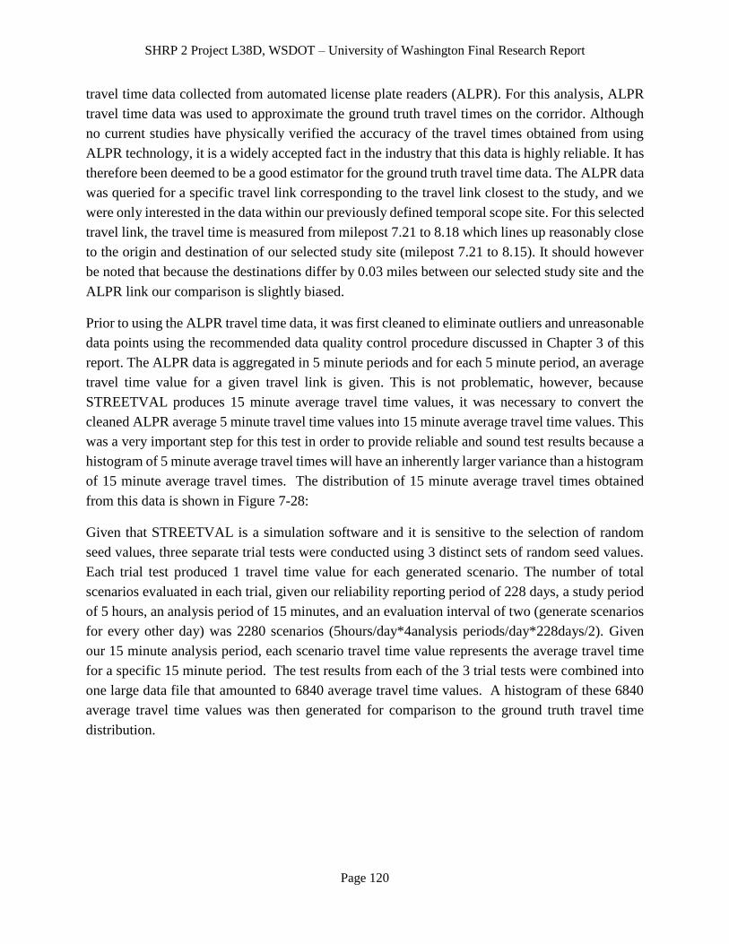
SHRP 2 Project L38D, WSDOT – University of Washington Final Research Report
Page 120
travel time data collected from automated license plate readers (ALPR). For this analysis, ALPR
travel time data was used to approximate the ground truth travel times on the corridor. Although
no current studies have physically verified the accuracy of the travel times obtained from using
ALPR technology, it is a widely accepted fact in the industry that this data is highly reliable. It has
therefore been deemed to be a good estimator for the ground truth travel time data. The ALPR data
was queried for a specific travel link corresponding to the travel link closest to the study, and we
were only interested in the data within our previously defined temporal scope site. For this selected
travel link, the travel time is measured from milepost 7.21 to 8.18 which lines up reasonably close
to the origin and destination of our selected study site (milepost 7.21 to 8.15). It should however
be noted that because the destinations differ by 0.03 miles between our selected study site and the
ALPR link our comparison is slightly biased.
Prior to using the ALPR travel time data, it was first cleaned to eliminate outliers and unreasonable
data points using the recommended data quality control procedure discussed in Chapter 3 of this
report. The ALPR data is aggregated in 5 minute periods and for each 5 minute period, an average
travel time value for a given travel link is given. This is not problematic, however, because
STREETVAL produces 15 minute average travel time values, it was necessary to convert the
cleaned ALPR average 5 minute travel time values into 15 minute average travel time values. This
was a very important step for this test in order to provide reliable and sound test results because a
histogram of 5 minute average travel times will have an inherently larger variance than a histogram
of 15 minute average travel times. The distribution of 15 minute average travel times obtained
from this data is shown in Figure 7-28:
Given that STREETVAL is a simulation software and it is sensitive to the selection of random
seed values, three separate trial tests were conducted using 3 distinct sets of random seed values.
Each trial test produced 1 travel time value for each generated scenario. The number of total
scenarios evaluated in each trial, given our reliability reporting period of 228 days, a study period
of 5 hours, an analysis period of 15 minutes, and an evaluation interval of two (generate scenarios
for every other day) was 2280 scenarios (5hours/day*4analysis periods/day*228days/2). Given
our 15 minute analysis period, each scenario travel time value represents the average travel time
for a specific 15 minute period. The test results from each of the 3 trial tests were combined into
one large data file that amounted to 6840 average travel time values. A histogram of these 6840
average travel time values was then generated for comparison to the ground truth travel time
distribution.
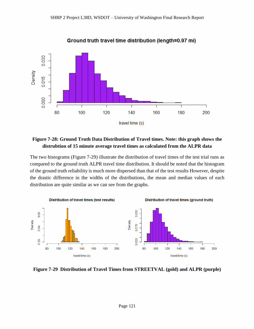
SHRP 2 Project L38D, WSDOT – University of Washington Final Research Report
Page 121
Figure 7-28: Ground Truth Data Distribution of Travel times. Note: this graph shows the
distrubtion of 15 minute average travel times as calculated from the ALPR data
The two histograms (Figure 7-29) illustrate the distribution of travel times of the test trial runs as
compared to the ground truth ALPR travel time distribution. It should be noted that the histogram
of the ground truth reliability is much more dispersed than that of the test results However, despite
the drastic difference in the widths of the distributions, the mean and median values of each
distribution are quite similar as we can see from the graphs.
Figure 7-29 Distribution of Travel Times from STREETVAL (gold) and ALPR (purple)
SHRP 2 Project L38D, WSDOT – University of Washington Final Research Report
Page 122
To further illustrate these results, Figure 7-30 shows the cumulative distribution of travel times for
the ground truth (shown in purple) compared to the test results (shown in gold). From this graph,
it can clearly be seen the test results tend to over predict the travel time for the lower probability
range, and under-predict travel times for the higher probability range (0.9 and greater). In addition,
the steepness of each curve is a good indicator of the travel time reliability. In this case, the slope
of the ground truth curve (gold) is much steeper than the purple curve which denotes a significantly
greater reliability than the actual reliability (purple). These results indicate that STREETVAL
provides an overoptimistic prediction of reliability.
Figure 7-30 Cumulative Distribution of Travel Times from STREETVAL (gold) and
ALPR (purple)
Figure 7-31 compares several common reliability performance measures, derived from the travel
time distributions for the ground truth travel time data, and the predicted test results.

SHRP 2 Project L38D, WSDOT – University of Washington Final Research Report
Page 123
Figure 7-31 Comparison of reliability performance measures between ground truth and
test results
From the results presented, it is clear that there is a large disparity between the predicted reliability
of STREETVAL and the actual reliability obtained from the ALPR data. There are many potential
explanations for this disparity. However, we believe that this error is most likely a result of a bias
in the estimation of the travel demand for each scenario. In STREETVAL, the travel demand is
estimated for each scenario using two main sources of information 1) 1 hour seed volumes 2)
AADT volume factors for each month, day of week, and hour of day. It is possible that the demand
from the seed day is not representative of the average demand on a given day and this may
introduce a small to very large bias in the software’s prediction. Another possibility for the large
discrepancy is that there is an additional factor that has not been accounted for which, if included,
would significantly decrease the prediction error. It is possible that better accounting
unpredictable driver behavior, accounting for variability in driver speed due to the presence of
traffic lights, or the glare caused by the reflection of the sun through the wind shield would improve
the prediction accuracy. It is also worth noting that this software was originally tested and shown
to work well for traffic in North Carolina, however, Seattle traffic and its drivers may be very
different. Additional model calibration may be necessary to see if for example, adjusting the
average headway or driver acceleration will significantly improve our results and help explain our
discrepancy.
7.10 Test Conclusion for STREETVAL
Based on our test results, it was shown that STREETVAL was unable to provide a reasonable
travel time reliability prediction for our urban arterial test site. The difference in variance and
widths of the ground truth travel time distribution, and the predicted travel time distribution from
STREETVAL is significant. Although our assessment of the software is biased due to a 0.03 mile
difference in the lengths of travel time links between the ground truth data and STREETVAL
Performance
Measure Ground Truth Test Results
5th percentile 90.3 110.8
10th percentile 93.0 112.2
80th percentile 117.7 123.0
85th percentile 121.3 124.4
95th percentile 133.7 127.6
mean 107.7 118.3
standard deviation 13.6 5.2
median 105.0 117.5

SHRP 2 Project L38D, WSDOT – University of Washington Final Research Report
Page 124
results, an only 3% margin of error is not sufficient to explain this large of a discrepancy. This
error is likely a result of both inaccurate demand prediction and not accounting for some principal
factor influencing travel times. A redeeming quality of the software, is that it was able to provide
a reasonable prediction for the mean and median travel times, differing by less than 10 percent.

SHRP 2 Project L38D, WSDOT – University of Washington Final Research Report
Page 125
CHAPTER 8 PILOT TESTING AND ANALYSIS ON SHRP 2 C11
PRODUCT
8.1 Introduction
Most benefit-cost analysis tools incorporate recurring congestion impacts and exclude non-
recurring (resulting from incident/weather/work zone/demand fluctuation) congestion impacts.
This is probably due to the difficulty of estimating non-recurring congestion impacts. The SHRP
2 program developed the C11 Reliability tool to facilitate estimating both recurring and non-
recurring congestion delays and their associated costs. The tool was applied to analyze the I-5
facility through the Joint Base Lewis-McChord (JBLM), also known as JBLM project.
8.2 Description of the Test Site
The research team has selected I-5 facility through the JBLM located between SR 510 (Marvin
Road NE) in Lacey and SR 512 in Lakewood for testing the travel time reliability tool. The test
site is in Pierce County, Washington State and is shown in Figure 8-1 (interchange locations are
indicated by green circles).
This portion of I-5 experiences congestion in both directions of travel particularly during evening
peak demand period. A congestion scan from INRIX is shown in Figure 8-2. INRIX data indicates
peak period congestion in both directions of travel between Dupont-Steilacoom Road and Thorne
Lane. Travel speed drops to as low as 35 mph in northbound direction during part of the evening
peak period.
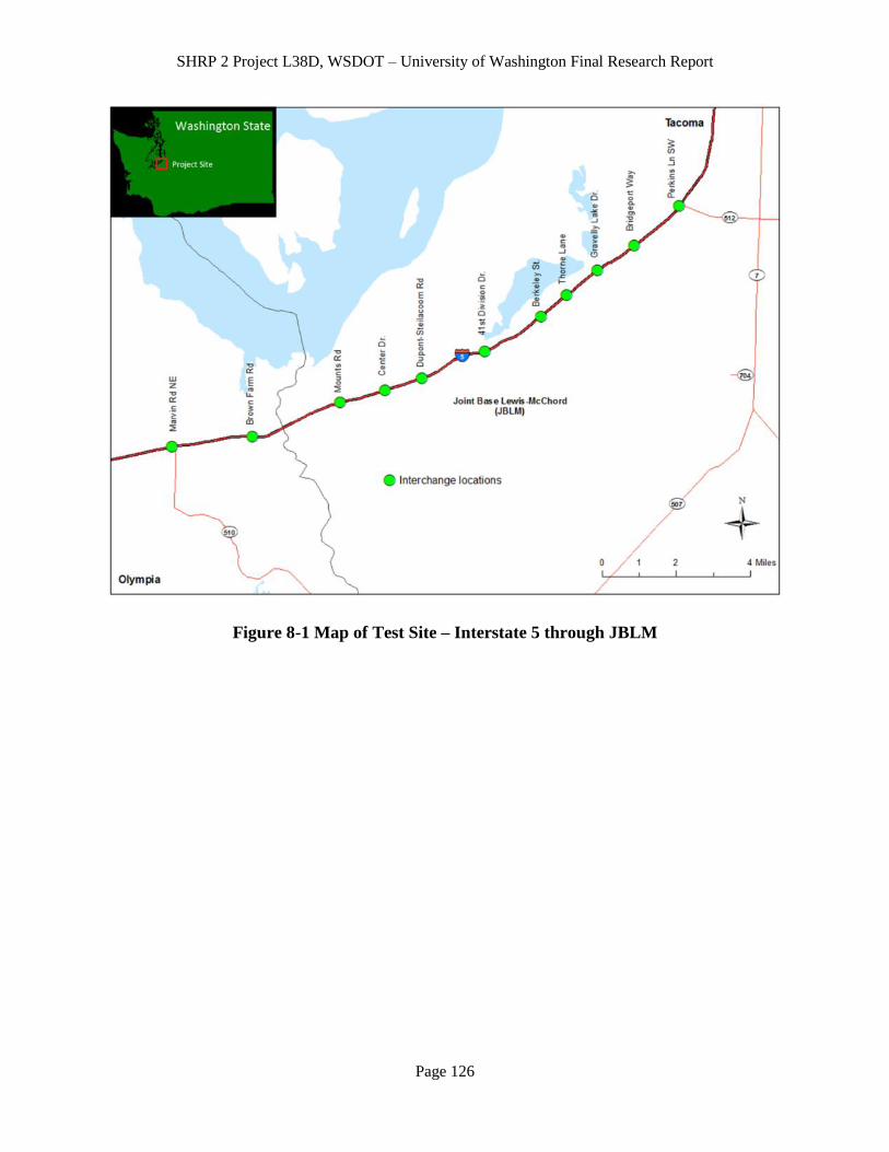
SHRP 2 Project L38D, WSDOT – University of Washington Final Research Report
Page 126
Figure 8-1 Map of Test Site – Interstate 5 through JBLM

SHRP 2 Project L38D, WSDOT – University of Washington Final Research Report
Page 127
Figure 8-2 INRIX Congestion Scan of I-5 JBLM Area
8.3 Alternatives to Test
To test the travel time reliability tool, existing condition (base case) and six conceptual alternative
improvements (scenarios) have been evaluated. These scenarios are:
1. Hard shoulder running between 41st Division Drive and Thorne Lane; and ramp metering
with HOV bypass at all interchanges between SR 510 and SR 512.
2. Extend 8 lanes from Berkeley Street interchange to Thorne Lane interchange; and
provide hard shoulder running between Mounts Road and Berkeley Street interchanges.
3. Add one lane each direction from Mounts Road to Thorne Lane.
4. Hard shoulder running from Mounts Road to Thorne Lane.
5. Ramp metering/increased incident response.
6. Ramp metering/increased incident response in combination with Option 4.
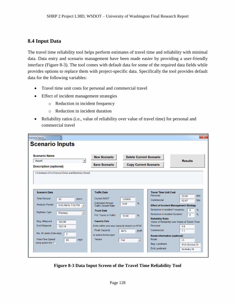
SHRP 2 Project L38D, WSDOT – University of Washington Final Research Report
Page 128
8.4 Input Data
The travel time reliability tool helps perform estimates of travel time and reliability with minimal
data. Data entry and scenario management have been made easier by providing a user-friendly
interface (Figure 8-3). The tool comes with default data for some of the required data fields while
provides options to replace them with project-specific data. Specifically the tool provides default
data for the following variables:
Travel time unit costs for personal and commercial travel
Effect of incident management strategies
o Reduction in incident frequency
o Reduction in incident duration
Reliability ratios (i.e., value of reliability over value of travel time) for personal and
commercial travel
Figure 8-3 Data Input Screen of the Travel Time Reliability Tool

SHRP 2 Project L38D, WSDOT – University of Washington Final Research Report
Page 129
The reliability tool allows evaluation of freeway mainline segments between interchanges. For this
pilot study, I-5 through JBLM area has been divided into 10 segments (Figure 8-4). Necessary
input data for these segments has been collected and/or generated using other tools. Reliability
ratios for personal and commercial travel are the default values from the travel time reliability tool.
Figure 8-4 Base Year (2012) Input Data
8.5 Output Data
The travel time reliability tool provides different performance metrics in an easy to understand
format which aids the users to interpret and communicate the results of analyses. For example, the
tool generates overall mean travel time index (TTI), 95 percentile TTI, 80 percentile TTI, 50
percentile TTI as well as proportion of trips below 45 and 30 mph speed (an example of output is
shown in Figure 8-5). Also performance measures are generated for base year and a future year
assuming an analysis period of 20 years.
In addition to performance metrics, the study team developed estimates of travel delay under each
conceptual scenario (Figure 8-6). The tool helps estimate congestion delays separately for both
personal and commercial travel. All improvement options show reduced congestion delays
compared to the base case indicating the tool is sensitive to roadway improvements. “Hard
shoulder running with ramp metering and increased incident response” provided most benefits in
terms of congestion delay reduction.
Begin End NB SBPersonal
Travel
Commercial
Travel
Reduction in
Incident
Frequency
Reduction in
Incident
Duration
Personal
Travel
Commercial
Travel
(mile) (mph) (%) (%) (pcph) (pcph) ($/hour) ($/hour) (%) (%)
I-5 Marvin Rd NE (SR 510) to Brown Farm Rd NE 112.01 114.18 2.17 3 3 60 99,000 1.21% 12.06 4875 4875 Level $22.66 $62.87 2.75 55 0.8 1.1
I-5 Brown Farm Rd NE to Mounts Rd 114.18 116.77 2.59 3 3 60 111,000 1.21% 11.77 4875 4875 Level $22.66 $62.87 2.75 55 0.8 1.1
I-5 Mounts Rd to Center Dr 116.77 118.02 1.25 3 3 60 120,000 1.21% 11.77 4875 4875 Level $22.66 $62.87 2.75 55 0.8 1.1
I-5 Center Dr to Dupont-Steilacoom Rd 118.02 119.07 1.05 3 3 60 121,000 0.84% 11.77 4875 4875 Level $22.66 $62.87 2.75 55 0.8 1.1
I-5 Dupont-Steilacoom Rd to 41st Division Dr 119.07 120.96 1.89 3 3 60 117,000 0.94% 11.77 4875 4875 Level $22.66 $62.87 2.75 55 0.8 1.1
I-5 41st Division Dr to Berkeley St 120.96 122.74 1.78 3 3 60 126,000 0.84% 10.08 4875 4875 Level $22.66 $62.87 2.75 55 0.8 1.1
I-5 Berkeley St to Thorne Lane 122.74 123.64 0.90 3 3 60 134,000 0.94% 10.08 4875 4875 Level $22.66 $62.87 2.75 55 0.8 1.1
I-5 Thorne Lane to Gravelly Lake Dr. 123.64 124.71 1.07 4 4 60 143,000 0.94% 10.08 6500 6500 Level $22.66 $62.87 2.75 55 0.8 1.1
I-6 Gravelly Lake Dr. to Bridgeport Way 124.71 125.92 1.21 4 4 60 140,000 0.94% 10.08 6500 6500 Level $22.66 $62.87 2.75 55 0.8 1.1
I-5 Bridgeport Way to SR 512 125.92 127.54 1.62 4 4 60 141,000 0.94% 10.08 6500 6500 Level $22.66 $62.87 2.75 55 0.8 1.1
I-5 Corridor - Marvin Rd to SR 512 112.01 127.54 15.53
Effect of Incident Mgt Reliability Ratio
Route LengthPosted
Speed
Annual
Traffic
Growth
Rate
Truck
Base Year
(2012)
AADT
Travel CostLanesARM
SegmentTerrain
Type
SB
Capacity
NB
Capacity

SHRP 2 Project L38D, WSDOT – University of Washington Final Research Report
Page 130
Scen
ari
o
Co
ng
es
tio
n
Me
tric
s
SR
510 t
o B
row
n
Fa
rm R
d
Bro
wn
Fa
rm R
d
to M
ou
nts
Rd
Mo
un
ts R
d t
o
Ce
nte
r D
r
Ce
nte
r D
r to
Du
po
nt-
Ste
ilaco
oo
m R
d
Du
po
nt-
Ste
ilaco
om
Rd
to
41st
Div
isio
n D
r
41st
Div
isio
n D
r to
Be
rkele
y S
t
Be
rke
ley
St
to
Th
orn
e L
an
e
Th
orn
e L
an
e t
o
Gra
velly L
ake D
r
Gra
velly L
ake D
r to
Bri
dg
ep
ort
Wa
y
Bri
dg
ep
ort
Wa
y
to S
R 5
12
2012
Base C
ase
Overall mean TTI 1.12 1.10 1.21 1.22 1.16 1.37 1.56 1.18 1.17 1.18
TTI95 1.37 1.34 1.66 1.67 1.51 1.99 2.39 1.53 1.51 1.51
TTI80 1.16 1.13 1.31 1.32 1.23 1.56 1.85 1.27 1.26 1.26
TTI50 1.07 1.05 1.15 1.15 1.10 1.29 1.48 1.14 1.13 1.13
% trips less than 45 mph 13.9% 13.3% 24.0% 24.5% 19.3% 32.6% 41.9% 18.4% 17.6% 17.7%
% trips less than 30 mph 2.3% 1.4% 4.5% 4.6% 2.7% 12.8% 23.1% 5.7% 5.5% 5.5%
Overall mean TTI 1.07 1.08 1.13 1.13 1.10 1.04 1.06 1.10 1.10 1.10
TTI95 1.25 1.29 1.42 1.43 1.34 1.14 1.21 1.32 1.31 1.31
TTI80 1.10 1.11 1.18 1.18 1.13 1.05 1.08 1.14 1.13 1.13
TTI50 1.04 1.04 1.07 1.08 1.05 1.02 1.03 1.06 1.06 1.06
% trips less than 45 mph 9.7% 11.3% 16.3% 16.5% 13.3% 5.4% 8.1% 12.2% 11.8% 12.0%
% trips less than 30 mph 1.2% 1.2% 1.8% 1.8% 1.4% 0.8% 1.0% 1.8% 1.7% 1.7%
Overall mean TTI 1.37 1.64 1.87 1.65 1.64 1.77 2.06 1.35 1.33 1.34
TTI95 1.99 2.58 3.06 2.60 2.58 2.86 3.42 1.96 1.92 1.93
TTI80 1.56 1.98 2.33 1.99 1.97 2.18 2.60 1.53 1.51 1.51
TTI50 1.29 1.55 1.77 1.56 1.55 1.68 1.94 1.28 1.26 1.27
% trips less than 45 mph 32.6% 47.6% 58.6% 48.0% 47.6% 54.1% 67.1% 31.9% 30.5% 30.9%
% trips less than 30 mph 12.7% 24.8% 33.5% 25.0% 24.8% 29.7% 37.0% 12.9% 12.5% 12.6%
Overall mean TTI 1.19 1.58 1.68 1.57 1.56 1.18 1.11 1.22 1.17 1.18
TTI95 1.60 2.44 2.68 2.42 2.39 1.52 1.36 1.64 1.54 1.56
TTI80 1.28 1.89 2.04 1.88 1.85 1.27 1.14 1.32 1.25 1.25
TTI50 1.13 1.49 1.59 1.49 1.48 1.13 1.06 1.16 1.11 1.12
% trips less than 45 mph 22.2% 43.4% 50.1% 43.0% 41.9% 18.2% 13.9% 22.9% 20.3% 20.8%
% trips less than 30 mph 3.7% 23.4% 25.9% 23.3% 23.0% 5.6% 1.5% 5.9% 3.0% 3.1%
2012
Base C
ase
2012
Scen
ari
o 1
2032
Base C
ase
2032
Scen
ari
o 1
Figure 8-5 Corridor Performance Indicators
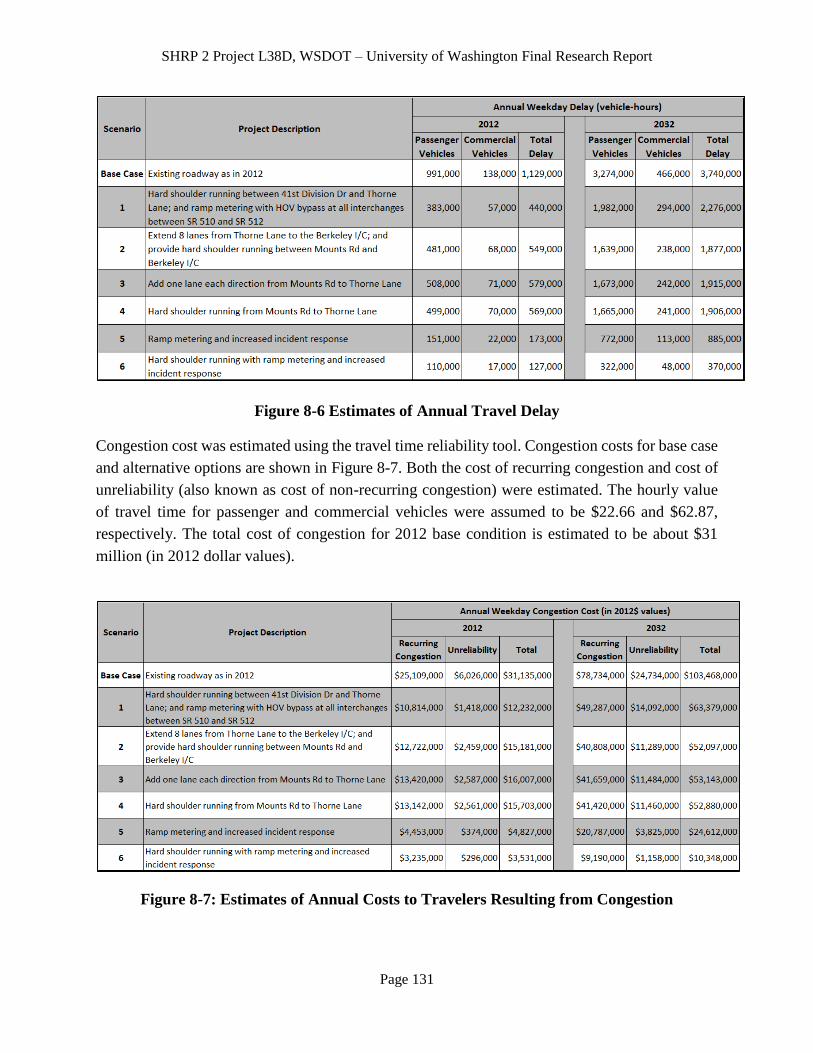
SHRP 2 Project L38D, WSDOT – University of Washington Final Research Report
Page 131
Figure 8-6 Estimates of Annual Travel Delay
Congestion cost was estimated using the travel time reliability tool. Congestion costs for base case
and alternative options are shown in Figure 8-7. Both the cost of recurring congestion and cost of
unreliability (also known as cost of non-recurring congestion) were estimated. The hourly value
of travel time for passenger and commercial vehicles were assumed to be $22.66 and $62.87,
respectively. The total cost of congestion for 2012 base condition is estimated to be about $31
million (in 2012 dollar values).
Figure 8-7: Estimates of Annual Costs to Travelers Resulting from Congestion

SHRP 2 Project L38D, WSDOT – University of Washington Final Research Report
Page 132
8.6 Cost of Alternatives
To perform economic analyses and compare project alternatives, it is necessary to estimate both
benefits and costs of alternatives. The travel time reliability tool help estimate travel time and
reliability benefits. Cost estimation of alternatives has been performed using WSDOT’s Planning
Level Cost Estimation (PLCE) tool.
PLCE is a database tool to perform cost estimation for projects that are very conceptual, often with
minimum or no design. The tool has been developed to estimate costs for varieties of projects
namely widening existing roadways or bridges, building new roads or bridges, modifying existing
interchanges or building new ones, improving intersections, and installing intelligent
transportation system (ITS).
PLCE utilizes unit price approach that accounts for regional differences as well as differences in
land use types and development density within a region. Since unit prices vary by geographic area,
separate unit prices are used in the estimate depending on where the project is located. Within each
geographic area, unit prices are again function of density of development such as rural, suburban,
urban, and dense urban.
The tool comes with default quantities per lane-mile for common items such as grading, drainage,
pavement, traffic control, etc. The underlying assumption of the methodology is that little or no
geotechnical data is known at the time of planning level estimate.
Furthermore, the tool comes with default unit costs obtained from historical data of WSDOT’s
past projects. Some unit prices were adjusted for differences in area prices, terrain (i.e., level,
rolling, or mountainous), ground conditions, and design assumptions. These unit costs can be
easily edited through user-friendly interfaces. An example of selecting project components to be
included in the estimation is shown in Figure 8-8.
A summary of estimated costs of alternatives is presented in Figure 8-9. Ramp metering and
incident response (Scenario 5) would cost the least while adding a lane each direction between
Mounts Road and Thorne Lane (Scenario 3) would cost the most. Scenario 3 requires addition of
two new lanes and reconstruction of a few interchanges and bridges resulting in much higher cost
compared to other scenarios.
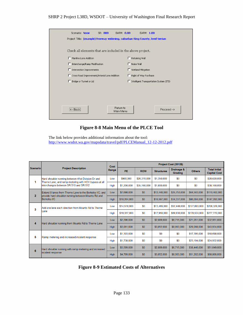
SHRP 2 Project L38D, WSDOT – University of Washington Final Research Report
Page 133
Figure 8-8 Main Menu of the PLCE Tool
The link below provides additional information about the tool:
http://www.wsdot.wa.gov/mapsdata/travel/pdf/PLCEManual_12-12-2012.pdf
Figure 8-9 Estimated Costs of Alternatives

SHRP 2 Project L38D, WSDOT – University of Washington Final Research Report
Page 134
8.7 Benefit-Cost Analysis
The travel time reliability tool performs an estimation of travel benefits. However, it does not
facilitate performing benefit-cost analysis incorporating project costs and benefits. This analysis
has been conducted outside the reliability tool using methodology in WSDOT’s benefit-cost
analysis tool (known as MP3B-C tool). This tool was found to be suitable for conducting benefit-
cost analysis for the type of projects being analyzed and available data.
A summary of the benefit-cost analysis is shown in Figure 8-10. The analysis was performed with
a set of assumptions that include:
An analysis period of 20 years
Annual discount rate of 4% (used to convert future costs and benefits to present values)
Benefits include travel time savings and reduction of unreliability
Personal and commercial travel time values are $22.66 and $62.87 per hour, respectively
Residual values were used to adjust the benefit/cost ratio to account for the value of the
improvement remaining after 20 years (the residual value methodology is based on work
done for AASHTO by the Texas Transportation Institute), and was done by applying the
following factors to the project’s estimated costs:
o Right of way - 0.45
o Grading and drainage - 0.40
o Structures - 0.43
o All other costs (including PE) – 0.00
Annual roadway O&M cost is $16,500 (in 2012$ values) per lane-mile
Annual IRT cost is $7,000 (in 2012$ values) per lane-mile
Annual signal/ramp meter O&M cost is $1,200 (in 2012$ values)

SHRP 2 Project L38D, WSDOT – University of Washington Final Research Report
Page 135
Figure 8-10 Summary of B-C Analysis
To prepare TIGER III Grant Application for I-5 JBLM project, WSDOT conducted an economic
analysis using TREDIS software. The total project benefit-cost ratio, based on anticipated project
design and construction costs, as well as all monetized benefits, including travel time, vehicle
operating costs, reliability, safety, freight and environmental, were estimated to range from 5.67
to 8.38. Travel time and reliability benefits were estimated to amount to $123.8 million
(undiscounted) for 24 years.
The travel time reliability tool provides estimates of benefits that include recurring congestion
reduction and reliability improvements. When analyzed the same JBLM project using the travel
time reliability tool with roadway capacity (2,190 pcphpl) from Highway Capacity Manual (as
suggested by the tool), benefit-cost ratio ranged from 1.96 to 2.43. Given this tool is considering
only direct benefits from travel time and reliability improvements, the values are expected to be
somewhat lower than those from analyses for TIGER III Grant Application (using TREDIS
software). However, the benefit-cost ratios from the travel time reliability tool seem to be too low
when compared with the values from TIGER III Grant Application.
When we analyzed the same JBLM project using the travel time reliability tool with reduced
roadway capacity (1,625 pcphpl), benefit-cost ratio ranged from 22.23 to 27.56. In this case, the
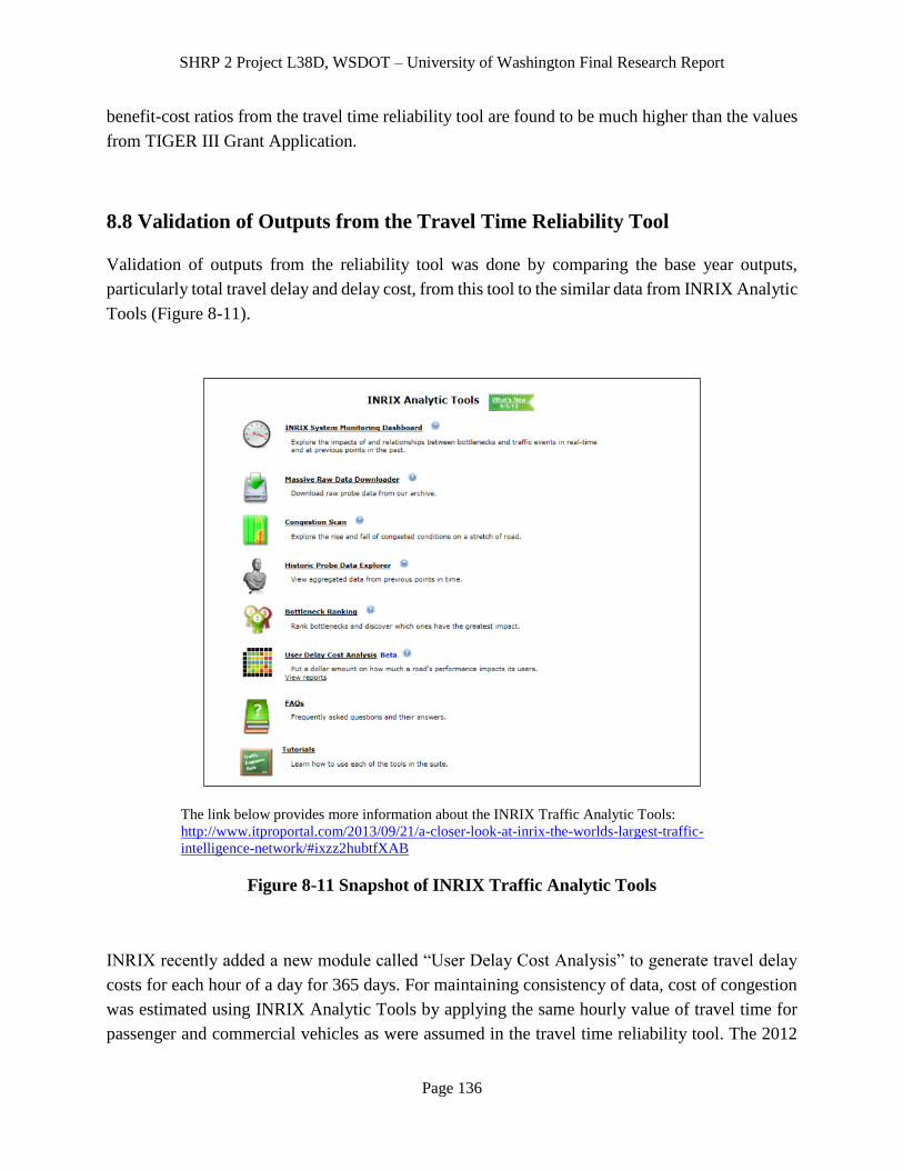
SHRP 2 Project L38D, WSDOT – University of Washington Final Research Report
Page 136
benefit-cost ratios from the travel time reliability tool are found to be much higher than the values
from TIGER III Grant Application.
8.8 Validation of Outputs from the Travel Time Reliability Tool
Validation of outputs from the reliability tool was done by comparing the base year outputs,
particularly total travel delay and delay cost, from this tool to the similar data from INRIX Analytic
Tools (Figure 8-11).
The link below provides more information about the INRIX Traffic Analytic Tools:
http://www.itproportal.com/2013/09/21/a-closer-look-at-inrix-the-worlds-largest-traffic-
intelligence-network/#ixzz2hubtfXAB
Figure 8-11 Snapshot of INRIX Traffic Analytic Tools
INRIX recently added a new module called “User Delay Cost Analysis” to generate travel delay
costs for each hour of a day for 365 days. For maintaining consistency of data, cost of congestion
was estimated using INRIX Analytic Tools by applying the same hourly value of travel time for
passenger and commercial vehicles as were assumed in the travel time reliability tool. The 2012
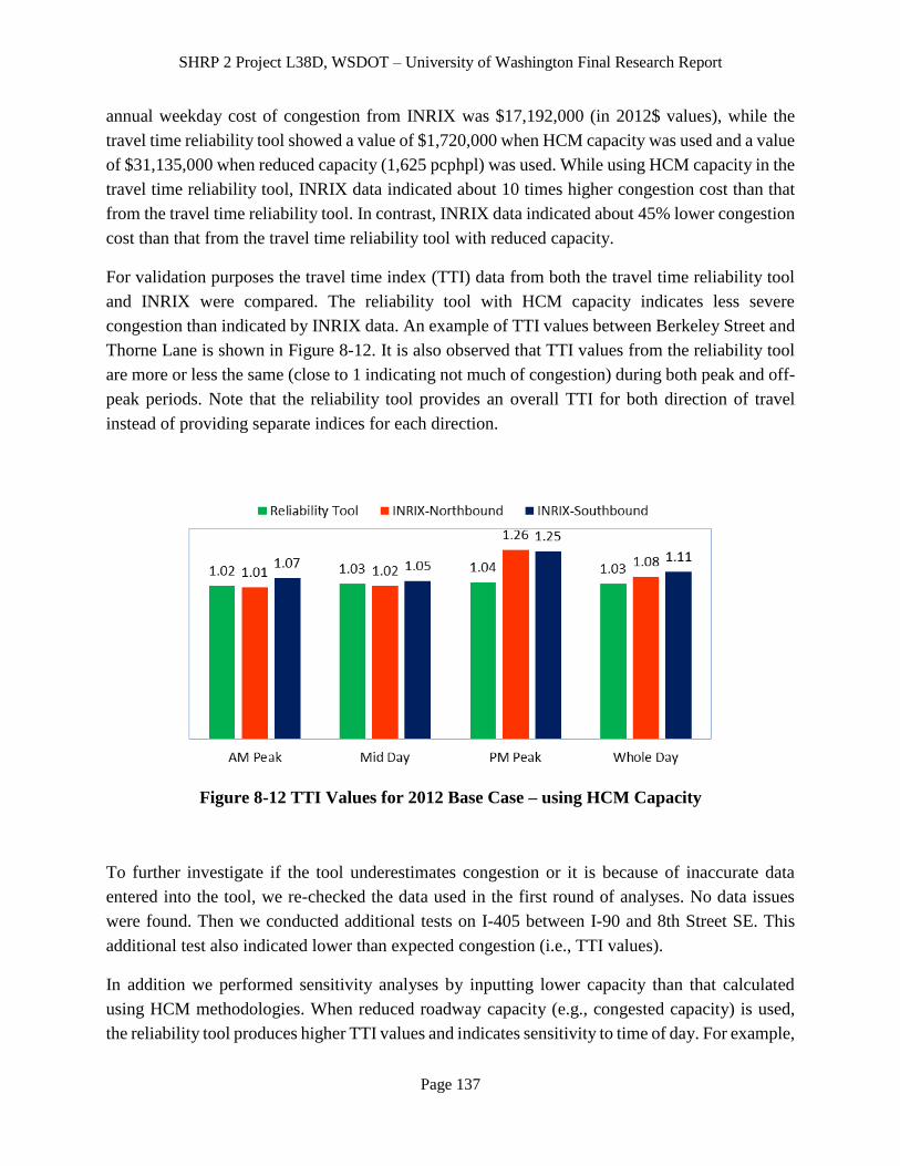
SHRP 2 Project L38D, WSDOT – University of Washington Final Research Report
Page 137
annual weekday cost of congestion from INRIX was $17,192,000 (in 2012$ values), while the
travel time reliability tool showed a value of $1,720,000 when HCM capacity was used and a value
of $31,135,000 when reduced capacity (1,625 pcphpl) was used. While using HCM capacity in the
travel time reliability tool, INRIX data indicated about 10 times higher congestion cost than that
from the travel time reliability tool. In contrast, INRIX data indicated about 45% lower congestion
cost than that from the travel time reliability tool with reduced capacity.
For validation purposes the travel time index (TTI) data from both the travel time reliability tool
and INRIX were compared. The reliability tool with HCM capacity indicates less severe
congestion than indicated by INRIX data. An example of TTI values between Berkeley Street and
Thorne Lane is shown in Figure 8-12. It is also observed that TTI values from the reliability tool
are more or less the same (close to 1 indicating not much of congestion) during both peak and off-
peak periods. Note that the reliability tool provides an overall TTI for both direction of travel
instead of providing separate indices for each direction.
Figure 8-12 TTI Values for 2012 Base Case – using HCM Capacity
To further investigate if the tool underestimates congestion or it is because of inaccurate data
entered into the tool, we re-checked the data used in the first round of analyses. No data issues
were found. Then we conducted additional tests on I-405 between I-90 and 8th Street SE. This
additional test also indicated lower than expected congestion (i.e., TTI values).
In addition we performed sensitivity analyses by inputting lower capacity than that calculated
using HCM methodologies. When reduced roadway capacity (e.g., congested capacity) is used,
the reliability tool produces higher TTI values and indicates sensitivity to time of day. For example,
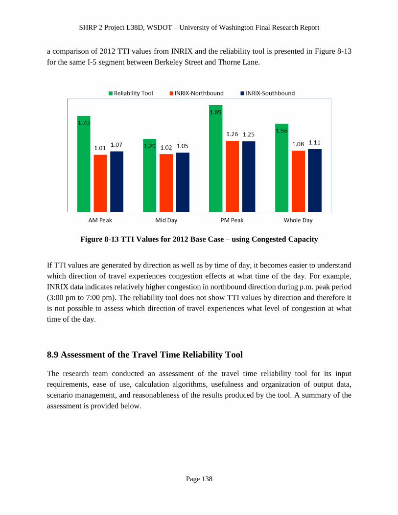
SHRP 2 Project L38D, WSDOT – University of Washington Final Research Report
Page 138
a comparison of 2012 TTI values from INRIX and the reliability tool is presented in Figure 8-13
for the same I-5 segment between Berkeley Street and Thorne Lane.
Figure 8-13 TTI Values for 2012 Base Case – using Congested Capacity
If TTI values are generated by direction as well as by time of day, it becomes easier to understand
which direction of travel experiences congestion effects at what time of the day. For example,
INRIX data indicates relatively higher congestion in northbound direction during p.m. peak period
(3:00 pm to 7:00 pm). The reliability tool does not show TTI values by direction and therefore it
is not possible to assess which direction of travel experiences what level of congestion at what
time of the day.
8.9 Assessment of the Travel Time Reliability Tool
The research team conducted an assessment of the travel time reliability tool for its input
requirements, ease of use, calculation algorithms, usefulness and organization of output data,
scenario management, and reasonableness of the results produced by the tool. A summary of the
assessment is provided below.

SHRP 2 Project L38D, WSDOT – University of Washington Final Research Report
Page 139
8.10 General Observations
The travel time reliability tool requires minimal data and appears to be easy to use. The tool has
been designed to require data that can be easily collected or assembled by those conducting a
sketch planning study. The required data can be acquired from widely used data sources.
The tool comes with simple and easy scenario management features. The tool facilitates analyses
of multiple scenarios by allowing creating and saving new scenarios with relative ease. The tool
displays results of the base and alternative scenarios side by side for ease of comparison.
This tool allows users to perform quick assessment of the effects of highway investments. It allows
conducting assessment of transportation investment benefits in terms of reducing recurring delay
as well as improving travel time reliability. Most of the existing economic analysis tools consider
only recurring delay, while exclude the effects of travel time reliability. Since this tool accounts
for this additional benefit from travel time reliability, it is expected to show more positive effects
of a highway investment on the economy than typical estimates using traditional tools and
methodologies.
The tool was tested on a wide range of improvement options. A few observations regarding the
analysis results are:
The tool estimates travel delay that is about one-tenth of the values from INRIX traffic
analysis tool. It seems like the tool underestimates travel impacts. This could be due to the
fact that the tool does not account for impacts from traffic volume other than mainline
volume, although ramp spacing and ramp traffic volume may have considerable effect on
freeway operations. Particularly the I-5 ramp traffic volume along JBLM is thought to be
the primary cause of congested condition along this stretch of the facility, but the tool does
not analyze the freeway mainline and ramps together as a system.
The travel time reliability tool uses three sets of hourly traffic distribution factors for peak
travel direction of a roadway. The tool selects one of these three sets based on
AADT/capacity ratio – less than 7.0, 7.1 to 11.0, and greater than 11.0. Base case and an
improvement option could sometimes have different AADT/capacity ratio leading to usage
of different set of hourly distribution factors, and thus an improvement option might
sometimes show worse traffic congestion than the base case.
For example, we had a 6-lane freeway segment with AADT of 111,000. The roadway
capacity (in this case we used congested capacity) for the base case was 9,750 pcph and
that of the improvement option was 10,285 pcph (assuming 5.5% increase of capacity
because of ramp meters and HOV bypass lanes). This combination of AADT and capacity
generates AADT/capacity ratios of 11.38 and 10.79 for the base case and the alternative.
These ratios lead to use of different hourly distribution sets for the base case and alternative
SHRP 2 Project L38D, WSDOT – University of Washington Final Research Report
Page 140
option resulting in higher TTI values for the alternative option (overall mean TTI values of
1.10 for the base case and 1.22 for the alternative option) even though the alternative option
has higher capacity and expected to reduce congestion. In this case, the tool indicates
congestion would increase even though traffic carrying capacity of the freeway is being
increased.
When used roadway capacity based on HCM (as suggested by the tool), the non-recurring
congestion delay appeared to be much higher than that of recurring congestion for all
improvement scenarios. However, when reduced roadway capacity was used, the tool
produced non-recurring congestion delay ranging from 8% to 19% for the scenarios which
is more in line with the expectation. Note that a 2003 report by Washington Transportation
Center (TRAC) titled “Measurement of Recurring versus Non-Recurring Congestion:
Technical Report” shows non-recurring congestion ranging from 5% to 58% depending on
type of estimate (e.g., conservative or liberal). This report is found at
http://www.wsdot.wa.gov/research/reports/fullreports/568.1.pdf.
8.11 Applicability
In assessing the tool a special attention was given to the applicability of the tool to evaluate various
improvement scenarios. An overview of our assessment follows:
The travel time reliability tool requires minimal data for performing assessment of impacts
of highway investments. Most of the data the tool requires seem to be relatively easy to
gather. So the tool can easily be used as a sketch planning tool for analysis of travel time
and reliability effects of some of the conceptual improvements typically analyzed as part
of planning studies.
In assessing travel benefits, the travel time reliability tool accounts for impacts of reduced
incident frequency and duration resulting from incident management strategies. However,
it does not provide any default input values or any sources/references to get help in
developing input data. The effects of incident management strategies have to be estimated
outside this tool and then entered as input into this tool.
The calculation methodology is directly applicable only to a roadway mainline (segments
between interchanges/intersections), not to improvements at roadway intersections,
interchanges and freeway ramps. Therefore it may not provide a comprehensive assessment
of transportation options because it does not perform analysis on a system of freeway
mainline, ramps and connecting roads accounting for vehicle interactions at the junctions.

SHRP 2 Project L38D, WSDOT – University of Washington Final Research Report
Page 141
The tool has been designed to evaluate roadway capacity improvements (e.g., adding lanes).
It does not come with a methodology to estimate benefits from varieties of transportation
improvement types including ITS improvements, demand management strategies, etc.
Therefore this tool does not seem to be applicable to analysis of all sorts of transportation
improvements typically considered by an agency.
This tool does not perform any benefit-cost analysis; it just produces travel time and
reliability benefits that can be used in a benefit-cost analysis. So for comparing alternatives,
further economic analyses need to be performed using other appropriate tools.
SHRP 2 Project L38D, WSDOT – University of Washington Final Research Report
Page 142
CHAPTER 9 CONCLUSIONS AND POTENTIAL
IMPROVEMENTS
9.1 Summary and Conclusions
In sum, the research team has tested and evaluated the analytical products from the SHRP 2
projects. The major conclusions for each product are summarized as follows:
The L02 methodology builds a strong foundation for travel time reliability monitoring. In this
project, travel time calculations and congestion data were acquired from single loop detectors at
five minute intervals. Non-recurring condition data for incidents and weather was taken from the
Washington Incident Tracking System and local weather stations. Plotting this data with
cumulative distribution functions provided a clear diagnosis for each route by analyzing
performance under congestion and non-recurring conditions and provides a strong framework for
comparison between routes. For example, comparing distributions for the alternative routes of
Interstate 5 and Interstate 405 in the Seattle Metro Area clearly highlighted that I-405 was more
reliable across various levels of congestion and non-recurring conditions. The use of L02 to
analyze reliability performance of roadway improvements was also tested and found to be quite
effective. However, this analysis was found to be most effective at a smaller scale than the route
level since these improvements often affect a much smaller portion of roadway. For example, the
I-405 Braided Ramps project that was tested modified approximately one mile of roadway.
Therefore, reliability performance measurement was scaled down to a three-mile segment, where
improvement in reliability across most conditions was clearly observed. Additionally, research
revealed that the cumulative distribution charts provided primarily qualitative reliability
information. The use of pie charts to show regime breakdown, and standard deviation of travel
time index to measure reliability improvements, were helpful in converting reliability information
to quantitative results. The most practical application for the L02 methodology and results was to
upload them to the DRIVE Net platform. DRIVE Net is an online tool where transportation
agencies and everyday commuters can view travel time reliability information for any route or
combination of routes. This accessible information can aid roadway improvement planning and
evaluation, and help drivers find the best commute routes.
For the pilot test of L07, various traffic data have been used, which include WSDOT DRIVE Net
Gray Notebook capacity analysis, single-loop detector data, traffic accident data and WSDOT
projects information. This study compared the measure of effectiveness, travel time index curve
and the benefit-cost analysis with the results computed based on empirical data. The test results
suggest that the tool tends to underestimate travel time under high traffic volumes and generate
over-optimistic measure of effectiveness and travel time index curves. The major findings are: 1)
the classification of treatment types is trivial and inefficient and the 15 types of very specific
SHRP 2 Project L38D, WSDOT – University of Washington Final Research Report
Page 143
treatments are unable to address actual projects; 2) it is difficult to define some parameters for the
treatment (e.g., the reduction of average accident clearance time) for the benefit-cost analysis; 3)
travel time reliability improvement only takes up a small portion of the total treatment benefit; 4)
the major benefits result from the reduction of number of accidents and the accuracy in estimating
the future accident number is the key factor influencing the benefit-cost analysis results; 5) the
detailed results and travel time index curves are inaccessible, which limits further comparison.
For FREEVAL, tests were conducted to verify tool accuracy for two different study sites in Seattle,
WA: an urban section of I-5 with a high ramp density, and a less urban section of I-405 with zero
ramps. Ground truth travel times for each study site were calculated from spot speed data collected
from dual loop detectors. The Gray Notebook procedure was used to calculate segment level travel
times from spot speeds. The results obtained from this study by comparing the predicted travel
time distribution outputted from FREEVAL to the ground truth travel times show that FREEVAL
tends to be over-optimistic in its predictions of travel times. A second test comparing results
between different seed days showed that the seed day does have an influence on the effect of the
results. This suggests that multiple trial runs using several different seed days may be necessary in
order to be confident in the test results. In sum, based on the testing results, FREEVAL does
provide a decent ballpark estimation of the actual distribution on travel times and hints that the
main sources and factors influencing travel time reliability have been accounted for by the tool.
In order to assess the accuracy of the STREETVAL software, a test was performed on an urban
arterial in Seattle, WA. Results from the test were obtained by comparing the predicted travel
times for the study facility outputted by the tool, to the actual travel times obtained from ALPR
data. The results show that the tool tends to under-predict the dispersion level of the travel time
distribution. The predicted travel time distribution is less dispersed than the actual travel time
distribution from the ALPR data, although the tool can reasonably predict the mean travel time.
The discrepancy in travel times suggests that some other factors (not accounted for) are influencing
the vehicle travel times. A few possible unaccounted factors are: 1) vehicle speeds may be different
than the posted speed limit and need to be properly calibrated for in the model; 2) vehicles slowing
down or speeding up to catch traffic lights; 3) vehicles may be blinded by the sun during the sunrise
and sunset hours and this could have an influence on the driver speed and segment travel times.
C11 accounts for travel time reliability as well as reoccurring congestion. It requires minimal data
for performing assessment of impacts of highway investments, and thus allows users to perform
quick assessment of the effects of highway investments. The tool comes with simple and easy
scenario management features. It facilitates analyses of multiple scenarios by allowing creating
and saving new scenarios with relative ease. The tool was tested to assess if it needs any further
improvements for enhancing its potential for use by transportation agencies. After extensive testing
on different improvement options, the project team developed a set of recommendations for further
improvement of the tool.

SHRP 2 Project L38D, WSDOT – University of Washington Final Research Report
Page 144
Detailed suggestions and potential improvements for each tool can be found in section 9.2.
9.2 Suggestions and Potential Improvements
9.2.1 Potential Improvements on SHRP 2 L02 Product
In general, the L02 is useful for outlining specifications for the data needed to create a TTRMS
system, guiding how to organize different conditions for the CDF, helping understand how to read
the CDF for impacts on delay, and identifying congestion sources for different corridors.
By testing the L02 procedure, the research team finds that there are limitations within the guide.
The events classified in the guide are listed as either weather or incident. However, there
is no category for “weather+incident” events. Because sometimes the cause of incidents
can be attributed to and exacerbated by adverse weather conditions, we believe that the
addition of a third “weather+incident” category is necessary. Guidance should also be
provided for when an event should be considered a combined “weather+incident” and
when these events should be considered separately.
The unique impact of each incident and weather event on travel time is hard to show by
grouping large amount of data into the CDF curves. It is certainly possible to make a large
number of curves and more specific nonrecurring conditions, such as collisions vs. disabled
vehicles and light rain vs. snow vs. fog. However, the data can only provide meaningful
curves if there are sufficient data points to plot for each regime. Thus, the guide should
help provide guides on when and how to establish TTRMS for different weather/incident
severities. The recommendations on the minimum sample size for drawing meaningful
curves are also needed.
The guide does not provide guides on the determination of route ends. For example, if
traffic design treatments are implemented on a segment, how should engineers choose the
length/boundary of the corridor for travel time reliability monitoring/analyzing relevant to
the design treatments?
The guide may consider including recommended methods to analyze the duration of the
impact of incidents, weather events (especially winter storm events), and other non-
recurring conditions and recognize that their impacts on travel reliability can extend past
the duration of the condition.
The guide should recommend using additional charts beyond the CDF for evaluating
reliability, especially where they can provide clearer quantitative information and help
guide policymakers in planning future roadway improvements.
The guide suggests analyzing for improvements at the route level; however improvements
are not generally implemented along the entire route, but rather in “hot spots” or
bottlenecks. Therefore, it is also necessary to analyze segment CDFs in addition to route-
SHRP 2 Project L38D, WSDOT – University of Washington Final Research Report
Page 145
level CDF’s when considering roadway modifications to improve reliability.
Recommended methods for TTRMS at the segment level would help identify areas
contributing the most to unreliability so that improvements can be targeted more precisely.
As a final note, the guide assumes the existence of a highly intelligent data collection system to
synthesize the data and make a TTRMS work effectively. For example, the I-5 facility could be
much better analyzed with a more extensive network of weather stations, especially those closer
to the roadway. Then this weather needs to be efficiently paired to each loop observation. Weather
conditions, such as brief downpours, can be very local in nature, and investing in a higher
resolution of weather data would make this system much more effective. Additionally, a system
with traffic detector data and incident data temporally and spatially connected can make it much
easier to analyze true impact of incidents. We expect that regions having data collection systems
with these (or similar) features will have the easiest time implementing the L02 methodology and
derive the greatest benefit from its results. Nevertheless, we have found it an effective guiding tool
for examining the travel time reliability in a greater detail of a region’s transportation network.
9.2.2 Potential Improvements on SHRP 2 L07 Product
The L07 tool has friendly interface and is easy to use. However, the software currently only
considers less commonly used design treatments for roadway segments. Based on the testing
results, the research team suggests the following potential tool/guide refinements for L07:
Add a COMPUTE button to allow the user to choose when to start the computation, so
that the software does not need to spend time computing every time when user changes a
single value.
Make the interface fit different computer resolutions. For example, if an 800*600
resolution screen is used (for most projectors), only the rows on the right and in the middle
can be shown.
Be able to predict travel time during peak hours more precisely, as the tool tends to
underestimate the effect of congestion.
Enable software to save results to a separate file and include more details about the results.
Consider the effect of combining multiple design treatments because in some instances 2
or more treatments may be implemented on the same site.
Present more detailed guidance for some default values such as event and work zone
characteristics, treatment effects.
Investigate further about the treatment effects including potential effects, and make the
coefficients in Figure 6-9 more open for modification.
Further consider effects of ramp metering on mainline flow. Due to its definition of
solutions, L07 may not be an ideal tool to estimate the effect of ramp metering. However,
it is possible for L07 to provide MOEs for these situations:

SHRP 2 Project L38D, WSDOT – University of Washington Final Research Report
Page 146
o Whether and how mid interchange off-ramps will affect traffic.
o How on-ramp design features will affect traffic flow. For example, different ramp
lengths and lane numbers will have different effects on mainline traffic condition.
o Effects of ramp spacing and interchange type on mainline flow.
9.2.3 Potential Improvements on SHRP 2 L08 Product
In general, the FREEVAL tool is a powerful simulation tool for evaluating different reliability
alternatives in association with various non-recurrent traffic events. However, because the tool
intends to cover as many aspects as possible, it requires multiple data sources and the input
procedure is complex. Below are potential improvements the research team found to be critical for
improving the FREEVAL tool.
Put all the tool guide information together for user reference. For now, users need to refer
to multiple reference documents that L08 provided to make sure all the steps are correctly
followed.
Disable the unnecessary options for the selection of the number of HCM segments and
disable the option of selecting non-basic segment types for the beginning and ending
segments.
Show alerts when steps are missing. For example, the software will keep working if user
fails to choose the ramp metering method. Another alternative is to show data input
summary, the model run will not be executed until user has confirmed the data entry is
complete.
Allow more flexible data input. Though using “seed day demand + demand multiplier table”
would save the user a lot of time inputting the data, it is time consuming for most engineers
to get the demand multiplier table.
Because the urban and rural defaults for the selection of demand ratios in the freeway
scenario generator are based on data from I-40, it is not accurate to apply these values to
other study locations because demand patterns are location-specific. Either this default data
option should be removed or it should be clearly noted that these values may not be valid
because they are based on one particular study location.
Most national holidays are on Mondays and Fridays. When we calculate the demand
multiplier, we found a large travel demand variation on these days. Our research team is
not sure whether we should use the holiday data to compute the multipliers or we just
consider these days as outliers and exclude them for the multiplier computing. Because of
this issue, we are unsure whether it will still be useful to include Mondays and Fridays. A
potential improvement to the software would be allowing users to select which work days
are included in the analysis.
To make the tool easier to use, there are a few aspects that could be improved for STREETVAL.
SHRP 2 Project L38D, WSDOT – University of Washington Final Research Report
Page 147
STREETVAL requires a large range of data input, we were unable to meet the necessary
data requirements demanded from using our multiple sources of loop and camera data.
Even if a complete set of demand data is available (most likely provided by imbedded loop
detectors) for each approach, and at each intersection along the study site, additional access
point demand data is still required to complete an analysis and this probably means
collecting data manually which is both a time consuming and a costly procedure. To avoid
this costly manual data collection procedure, the tool should offer a method to estimate
access point demand data and seed demand data.
Other improvements could be made to the procedure itself since this can be confusing for
a first time user. Providing the user with steps with clearly defined tasks would make this
tool much easier and friendly to the user. The FREEVAL software is good in this respect;
each task was a specific task that the user could follow consecutively in order to complete
an analysis. Also, the aesthetics of the interface require some touch-ups and a few glitches
such as the malfunctioning buttons and floating spreadsheet numbers.
9.2.4 Potential Improvements on SHRP 2 C11 Product
The travel time reliability estimation tool was tested to assess if the tool needs any further
improvements for enhancing its potential for use by transportation agencies. After extensive testing
on different improvement options, a set of recommendations have been developed for further
improvement of the tool. These are:
All three sub-tools - the travel time reliability, market access and intermodal connectivity
tools - could be designed as a coordinated suite with provisions to use them individually,
if desired. This would allow easily combining the benefits from all these tools for use in
further economic analyses. It would be more useful if the tool performs benefit-cost
analysis by taking necessary information from a user about project’s capital and O&M
costs, and other benefits calculated outside this tool.
The tool is found to underestimate TTI values. We recommend revisiting the calculation
methodology and assumptions. We also recommend modifying the tool to provide TTI and
other performance metrics by direction of travel and time of day.
The tool takes input for incident reduction frequency and duration, instead of helping
estimate or suggesting values for these inputs. The tool does not suggest which
tools/methodologies to use to estimate incident reduction frequency and duration. The
study team recommends adding some suggestions about what tool can be used to generate
these inputs or providing a set of default values to choose from depending on improvement
types being analyzed.

SHRP 2 Project L38D, WSDOT – University of Washington Final Research Report
Page 148
The input to the tool does not distinguish between types of trucks (e.g., light, medium and
heavy trucks). Instead of using proportion of different truck types, the tool uses an overall
percent of trucks in the vehicle mix. To capture travel impacts more accurately, the study
team recommends performing analysis by taking truck classification into accounts. It is
also recommended to use the values of time for light, medium and heavy trucks. These
modifications would improve quality of assessment of travel time reliability and congestion
costs.
For all multilane and signalized highways, the tool derives two-way capacity from one-
way capacity (input by users) by assuming symmetrical geometry on both directions of
travel. Two directions of a highway segment are not always similar in terms of geometry
and other characteristics affecting capacity. Therefore it may not be always appropriate to
derive two-way capacity from one-way data. We recommend modifying the tool to
accommodate input for both directions of travel and perform calculations by directions.
The study team recommends allowing input of hourly traffic volume in addition to AADT
to facilitate calculation of travel delay and its economic impacts for any desired time of
day (e.g., a.m. or p.m. peak hour). This will help assess travel impacts for any time period
of a day.
Hourly traffic volume plays an important role in calculating 24-hour delay and associated
costs to travelers. The temporal distribution of traffic varies by corridor (and even by
specific locations within a corridor) based on land use type, employment, etc. We suggest
modifying the tool to allow making changes to the default hourly factors that comes with
the tool. Thus users would have two options – either use the default values or enter project
specific temporal distribution data (if available).
The tool provides an option to select an analysis period (i.e., time of day) from four
exclusive options (6:00 a.m. to 9:00 a.m., 9:00 a.m. to 3:00 p.m., 3:00 p.m. to 7:00 p.m.
and 6:00 a.m. to 7:00 p.m.). It does not include night in the analysis. Also it does not allow
selecting two or more time periods (for example both a.m. and p.m. peak periods) for
analysis. To analyze peak demand periods, the tool needs to be run separately for each of
the peak periods (e.g., a.m. peak or p.m. peak periods). We suggest expanding the list of
analysis periods to include “Night” and “Daily” as options as well as allowing selecting
multiple time periods for a single run.
The tool provides options to either directly enter capacity calculated based on HCM
methodology or simply selecting a terrain type (i.e., flat, rolling or mountainous)
representing the project. When terrain is selected, the algorithm in the tool estimates peak
capacity assuming values for other parameters needed for calculations. This capacity
calculation could be made more rigorous by taking lane width, shoulder width and other
necessary data from users.

SHRP 2 Project L38D, WSDOT – University of Washington Final Research Report
Page 149
The tool comes with analysis capability of only a uniform segment of a roadway between
two interchanges or signals. It would be more useful if the scope of the tool is expanded to
include multiple segments containing interchanges/signals in-between or network of
roadways with different geometric and traffic conditions.
For a relatively long stretch of a roadway, the tool’s architecture requires dividing the
roadway into a number of segments within the scope of a scenario because the tool analyzes
only segments between two adjacent interchanges and/or signal controls. In such cases, the
tool takes inputs and produces outputs for each segment separately. It would be helpful if
the tool summarizes the outputs by combining the data from all the segments.
The current version of the tool provides annual weekday delays and congestion costs. The
project team recommends modifying the tool to provide annual output for weekdays and
weekends. It is also recommended to produce output by hour of day. This will allow
performing analyses by time of day (peak hour, peak period, daily, etc.), if necessary.
The tool comes with default values of reliability ratios (i.e., value of reliability over value
of travel time) for personal and commercial travel. These ratios may vary by geographic
location (e.g., state, region, county, city, or a subarea) of the project. It is suggested to
provide links to references (if any research materials are available) with possible range of
default values so that a user can choose values appropriate for the geographic location of
the project to analyze.
The tool does not take any input to specify which the base year is, instead the tool assumes
the current year as the base year. This assumption may not hold for all cases. The study
team recommends modifying the input screen to allow users to enter the base year of
analysis.
9.3 Future Works
After completing this project, the research team has found that there are some opportunities for
future testing and work on SHRP 2 reliability products. The future works are listed below.
Evaluate alternative sources of travel time data such as INRIX and Bluetooth tracking.
Other accurate sources of travel time data (i.e., INRIX and Bluetooth detection data) can
be used as alternatives of the travel times generated from single loop detectors, although
these new travel time data are not as readily available for L02. INRIX provides travel time
data collected from motorists that are using its navigation services. Bluetooth detection
technology also has the ability to measure travel times by tracking cell phones and other
devices. Although detectors are currently not widespread enough for network-level travel
SHRP 2 Project L38D, WSDOT – University of Washington Final Research Report
Page 150
time calculation, this is an excellent emerging technology that can be applied for reliability
research.
Apply L02 methodology to signalized highways and arterials to evaluate travel time
reliability. Travel time data from single loop detectors does not transfer well from freeways
to signalized highways and arterials, as it uses two point speeds and assumes an average
speed to calculate segment travel times. This assumption is invalid for the signalized
highways and arterials. However by using INRIX or Bluetooth data for travel time
calculation, travel time reliability can easily be measured for roadways other than freeways.
Expand access to travel time reliability information by advancing the DRIVE Net platform.
Access to reliability information for transportation agencies and drivers can be expanded
by increasing the quality and quantity of the data provided on online platforms such as
DRIVE Net. By acquiring travel time data from Bluetooth detectors and/or INRIX, the data
may be more accurate, reliable, and available for many more roadways. This will enable
much more personalized reliability data. Making this additional data available on DRIVE
Net and expanding the reliability visualization tools available to users will help create a
more reliable, efficient transportation network.
The testing of L07 tool mainly focuses on freeways since the loop detector data is available
for calculating travel time reliability. Many roadway treatments provided in the L07 tool
are designed for highways, where the required traffic data is not available for this project.
Thus, the findings and results generated from the analysis for freeway systems are not
directly applicable to highways. By acquiring appropriate traffic data, the benefit-cost
analysis of roadway treatments for highways can be conducted. Moreover, if L07 can
provide more details about the tool results, the effectiveness of the algorithm can be also
examined.
For testing of FREEVAL, ground truth travel times were calculated from spot speed data
generated from loop detector sensors. Travel times collected from automated license plate
reader cameras were used as the source of ground truth data for STREETVAL. For the
future work, other sources of data might also be used for the same purpose such as
dedicated short range communication device data such as Wi-Fi and Bluetooth as well as
a probe vehicle data source.
SHRP 2 Project L38D, WSDOT – University of Washington Final Research Report
Page 151
References
ASTM E2665-08. Standard Specification for Archiving ITS-Generated Traffic Monitoring Data.
ASTM International, West Conshohocken, PA, 2008.
Athol, P., Interdependence of certain operational characteristics within a moving traffic stream.
Highway Research Record 72, Transportation Research Board, Washington, DC, 58–87,
1965.
Cambridge Systematics. Analytical Procedures for Determining the Impacts of Reliability
Mitigation Strategies, Transportation Research Board. 2010.
Cambridge Systematics. Incorporating Reliability Performance Measures into the Transportation
Planning and Programming Processes. SHRP 2 Reliability Project L05. 2013.
Chen, C., J. Kwon, J. Rice, A. Skabardonis, and P. Varaiya. Detecting Errors and Imputing Missing
Data for Single-Loop Surveillance Systems. Transportation Research Record: Journal of the
Transportation Research Board, No. 1855. Transportation Research Board of the National
Academies, Washington, D.C., 2003, pp. 160-167.
Corey, J., Y. Lao, J. Wu and Y. Wang, Detection and Correction of Inductive Loop Detector
Sensitivity Errors Using Gaussian Mixture Models, Transportation Research Record:
Journal of the Transportation Research Board, No. 2256, pp.120-129, 2011.
Economic Development Research Group . Development of Tools for Assessing Wider Economic
Benefits of Transportation. SHRP 2 Reliability Project C11. 2013.
INRIX, INRIX Traffic Data Services: Tapping into Real-time Traffic Flow, Accessed online
http://cta.ornl.gov/TRBenergy/trb_documents/2012_presentations/192_%20T%20Trepanier
%20-%20INRIX%20LeeSchipper%20Data%20Workshop%20TRB2012.pdf on August, 14,
2013.
Institute for Transportation Research and Education. Establishing Monitoring Programs for Travel
Time Reliability. SHRP 2 Reliability Project L02. 2013.
Ishimaru, J. M., and M. E. Hallenbeck.. FLOW Evaluation Design Technical Report., WA.RD
466.2, 1999.
Kimley-Horn and Associates, Inc. Integrating Business Processes to Improve Travel Time
Reliability. Transportation Research Board, 2011.
Kittelson and Associates, Inc. Incorporation of Travel Time Reliability into the HCM. SHRP 2
Reliability Project L08 Final Report, 2013.

SHRP 2 Project L38D, WSDOT – University of Washington Final Research Report
Page 152
Parsons Brinckerhoff, & Delcan Corporation. Institutional Architectures to Improve Systems
Operations and Management. Transportation Research Board, 2012
Potts, I. B., Harwood, D. W., Hutton, J. M., Fees, C. A., Bauer, K. M., Kinzel, C. S., and Frazier,
R. J. Identification and Evaluation of the Cost-Effectiveness of Highway Design Features to
Reduce Nonrecurrent Congestion. No. SHRP 2 Reliability Project L07. 2013.
Texas Transportation Institute, Quality Control Procedures for Archived Operations Traffic Data:
Synthesis of Practice and Recommendations – Final Report, Prepared for Office of Highway
Policy Information, FHWA, March 2007
Turner, S., R. Margiotta, and T. Lomax. Monitoring Urban Freeways in 2003: Current Conditions
and Trends from Archived Operations Data, Report No. FHWA-HOP-05-018, December
2004
Wang Y., M. Hallenbeck, and P. Cheevarunothai. Quantifying incident-induced travel delays on
freeways using traffic sensor data. Technical report, Transportation Northwest, University of
Washington, 2008.
Wang, Y., X. Ma, S. Xiao, Y. Malinovskiy, J. Corey, and K. Henrickson. Digital Roadway
Interactive Visualization and Evaluation Network Applications to WSDOT Operational Data
Usage. Technical report. 2013