Fiber Optical Communication - ttu.ee 1.pdf · Fiber Optical Communication Lecture 1, Slide 2...
35
Fiber Optical Communication Lecture 1, Slide 1 Fiber Optical Communication Examiner/lectures: Prof. Peter Andrekson [email protected] , +372 – 5558 7388; +46 – 70 3088 606 Laboratory exercises: Egon Astra [email protected] , +372 – 5560 2230
Transcript of Fiber Optical Communication - ttu.ee 1.pdf · Fiber Optical Communication Lecture 1, Slide 2...

Fiber Optical Communication Lecture 1, Slide 1
Fiber Optical Communication
Examiner/lectures:
Prof. Peter Andrekson
[email protected], +372 – 5558 7388; +46 – 70 3088 606
Laboratory exercises:
Egon Astra
[email protected], +372 – 5560 2230
Fiber Optical Communication Lecture 1, Slide 2
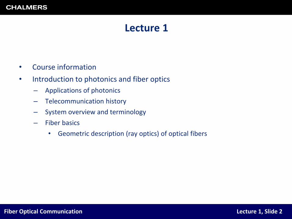
Lecture 1
• Course information
• Introduction to photonics and fiber optics
– Applications of photonics
– Telecommunication history
– System overview and terminology
– Fiber basics
• Geometric description (ray optics) of optical fibers

Fiber Optical Communication Lecture 1, Slide 3
• The book that is used is very well known…
• …and in the fourth edition
• Govind P. Agrawal: Fiber-Optic Communication Systems, ISBN: 9780470505113
Course outline• Lectures:
- ca 13 in total + repetition
• Lab exercises
• Home assignments
• Exam on xxx

Fiber Optical Communication Lecture 1, Slide 4
Course objectivesAfter completion of this course, the student should be able to
• Describe the fundamental properties and limitations of fiber-optic systems
• Describe and analyze the most important system components and their limitations: transmitters, fibers, receivers, optical amplifiers
• Evaluate a proposed system design and understand the trade-offs
• For optical transmitters: Understand different implementations, primarily using external modulators
• For optical fibers: Quantify dispersion, attenuation, and to some extent nonlinearities as well as their impact on signal transmission
• For optical receivers: Analyze receivers with and without optical pre-amplifier, know all relevant noise mechanisms, evaluate the bit error rate
• For optical amplifiers: Understand the fundamental properties of erbium-doped fiber amplifiers and quantify the impact of using them
• For systems: Evaluate different implementations such as wavelength division multiplexing and time division multiplexing.
Fiber Optical Communication Lecture 1, Slide 5
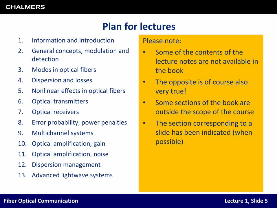
Plan for lectures1. Information and introduction
2. General concepts, modulation and detection
3. Modes in optical fibers
4. Dispersion and losses
5. Nonlinear effects in optical fibers
6. Optical transmitters
7. Optical receivers
8. Error probability, power penalties
9. Multichannel systems
10. Optical amplification, gain
11. Optical amplification, noise
12. Dispersion management
13. Advanced lightwave systems
Please note:
• Some of the contents of the lecture notes are not available in the book
• The opposite is of course also very true!
• Some sections of the book are outside the scope of the course
• The section corresponding to a slide has been indicated (when possible)

Fiber Optical Communication Lecture 1, Slide 6
Information about the homepage
• There is a course homepage http://lr.ttu.ee/irm0120/
• Will eventually contain
– News
– Lecture notes
– Home assignments
– Lab instructions

Fiber Optical Communication Lecture 1, Slide 7
Some photonic applications
LED-TV
LED light bulb
Blu-Ray disc
Solar cellOptical communication
Fiber-optic gyroscope
Environmental monitoring

Fiber Optical Communication Lecture 1, Slide 8
Some photonic applications• Telecommunication
– Lasers, modulators, fibers, detectors for communication systems
– Free-space optical links
• Information and Communication Technology
– CCD and CMOS sensors for imaging
– Data storage and retrieval (CD, DVD, BluRay)
– Optical interconnects (mainly in high performance computing context today)
• Sensors and spectroscopy
– ”Smart cameras” for image processing/machine vision
– Many, many applications, including sensors for measuring:
• Position, distance, thickness etc.
• Angular rate (ring laser/fiber gyroscopes)
• Gas concentration (using absorption)

Fiber Optical Communication Lecture 1, Slide 9
Some photonic applications• Security
– Intrusion detection
– Laser radar (LIDAR)
• Lighting
– LEDs for indoor lighting
– LEDs and Lasers for artistic lighting
• Energy
– Solar cells
• Biophotonics
– Optical tweezers, optical scalpels
– Optical tomography
• Military
– Surveillance
– Weapon guidance
– Countermeasures and laser guns

Fiber Optical Communication Lecture 1, Slide 10
The motivation: the Internet• Figure shows number of hosts connected to the Internet
– Around 109 hosts...
• Traffic grows quickly
– How to keep up with the increasing demand?
Fiber Optical Communication Lecture 1, Slide 11
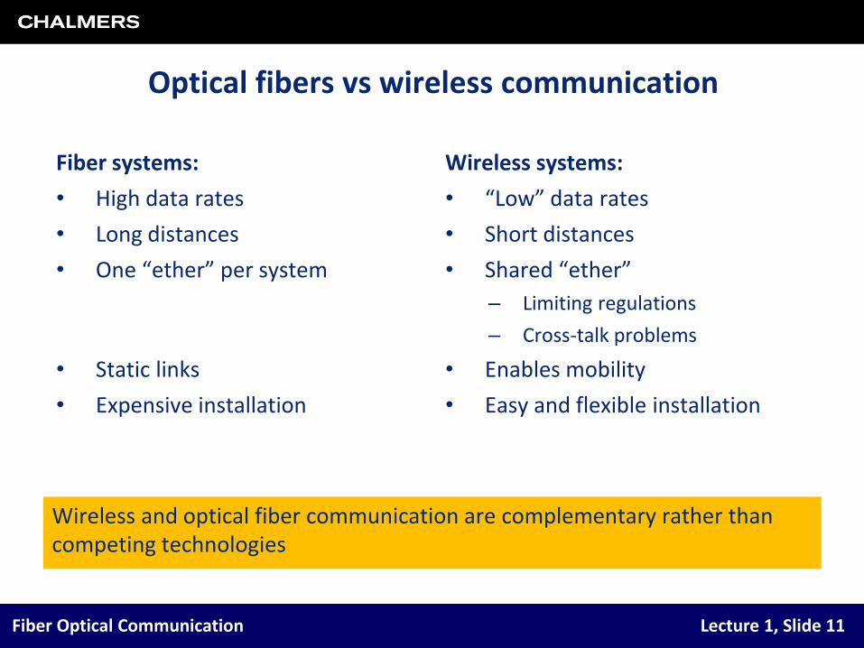
Optical fibers vs wireless communication
Fiber systems:
• High data rates
• Long distances
• One “ether” per system
• Static links
• Expensive installation
Wireless systems:
• “Low” data rates
• Short distances
• Shared “ether”
– Limiting regulations
– Cross-talk problems
• Enables mobility
• Easy and flexible installation
Wireless and optical fiber communication are complementary rather than competing technologies

Fiber Optical Communication Lecture 1, Slide 12
Transatlantic cables
Fibers are used for high speed, long haul communication, but also for:
• Intercity connects and city networks
• Providing high speed connections to terminals providing wireless services
• High speed (100 Mbit/s and above) services FTTx, where x = home etc.
A submarine cable1. Polyethylene2. Mylar tape3. Stranded steel wires4. Aluminum water barrier5. Polycarbonate6. Copper or aluminum tube7. Petroleum jelly8. Optical fibers
The continents are today connected by fiber-optical communication links

Fiber Optical Communication Lecture 1, Slide 13
The electromagnetic spectrum
Frequency: ν ≈ 200 THz
Wavelength: λ, typ. 1.55 μm
Light velocity in vacuum:
c ≈ 2.998×10⁸ m/s
The carrier frequency is much higher in lightwave systems than in microwave systems
Lightwave systems typically use infrared light
Frequency Wavelength
1018 Hz
1 THz
1 GHz
1 MHz
1 µm
1 nm
1 mm
1 m
1 km
Photon energy
1 eV
1 keV
1 meV
10-6 eV
10-9 eV
ultra-violet
infrared
x-ray
mm-waves
microwaves
radio waves
1015 Hz visible

Fiber Optical Communication Lecture 1, Slide 14
Properties of optical fibersAdvantages:
• Low attenuation (0.2 dB/km)
• Large bandwidth (1.55 μm–1.3 μm = 250 nm > 30 THz)
• Low weight, compact, flexible
• Isolated from the environment
– No crosstalk from other fibers or microwave sources
• Low sensitivity to environmental conditions
– Can operate on the ocean floor
– Immune to electromagnetic interference
• Provides electrical isolation between terminals
– No ground loops, damage cannot cause sparking
Disadvantages:
• Not wireless, installation is costly and slow
• Hardware is expensive compared to mass-produced electronics
Fiber Optical Communication Lecture 1, Slide 15
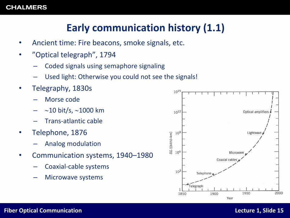
Early communication history (1.1)• Ancient time: Fire beacons, smoke signals, etc.
• ”Optical telegraph”, 1794
– Coded signals using semaphore signaling
– Used light: Otherwise you could not see the signals!
• Telegraphy, 1830s
– Morse code
– 10 bit/s, 1000 km
– Trans-atlantic cable
• Telephone, 1876
– Analog modulation
• Communication systems, 1940–1980
– Coaxial-cable systems
– Microwave systems

Fiber Optical Communication Lecture 1, Slide 16
Optical Communication History
1962 First semiconductor laser (GE, IBM, Lincoln Lab)
1966 First optical fiber, loss: 1000 dB/km (Corning Glass)
1970 Fiber with an optical attenuation of 20 dB/km (Corning Glass)
1970 AlGaAs-lasers operating at room temperature
1982 0.16 dB/km (theoretical limit) single-mode fiber
1986 First erbium-doped fiber optical amplifier
1988 Trans-Atlantic and trans-Pacific cable systems (565 Mbit/s)
1995 Repeaterless trans-oceanic systems (5 Gbit/s)
1997 Commercial WDM systems
2004 Multiple band transmission (S + C + L)
2007 “Advanced” nonbinary formats; 40 Gbit/s systems

Fiber Optical Communication Lecture 1, Slide 17
Optical Communication History• First generation, 1980
– GaAs lasers, 0.8 μm, 45 Mbit/s, using electrical repeaters
• Second generation
– InGaAsP lasers, 1.3 μm (minimum dispersion), 100 Mbit/s
– Single-mode fibers, 2 Gbit/s over 44 km in 1981
• Third generation, 1.55 μm (minimum loss)
– Dispersion-shifted fibers
– Single longitudinal mode lasers
– Still using electrical repeaters
• Fourth generation
– Optical amplification
– Wavelength-division multiplexing (WDM)
• Fifth generation
– Increased spectral range
– Increased spectral efficiency

Fiber Optical Communication Lecture 1, Slide 18
Progress in lightwave communication
The bit rate-distance product has increased eight orders of magnitude

Fiber Optical Communication Lecture 1, Slide 19
Progress in lightwave communication
Efforts have been made to:
• Increase the data rate per channel
• Increase the number of channels
• Increase the distance between repeaters
– Or at least keep it from shrinking when increasing other parameters
Rapid progress has been made, laboratory systems show the way forward

Fiber Optical Communication Lecture 1, Slide 20
A fiber-optic communication link
optical pre- amplifier
photo- detector
semiconductor laser
optical modulator
optical fiber
electrical signal
optical signal
optical receiver
electronicsoptical
transmitter
optical amplifier
optical fiber
optical fiber
optical transmitter
optical receiver
repeater
information receiver
receiver electronics
information source
drive electronics
Fiber Optical Communication Lecture 1, Slide 21
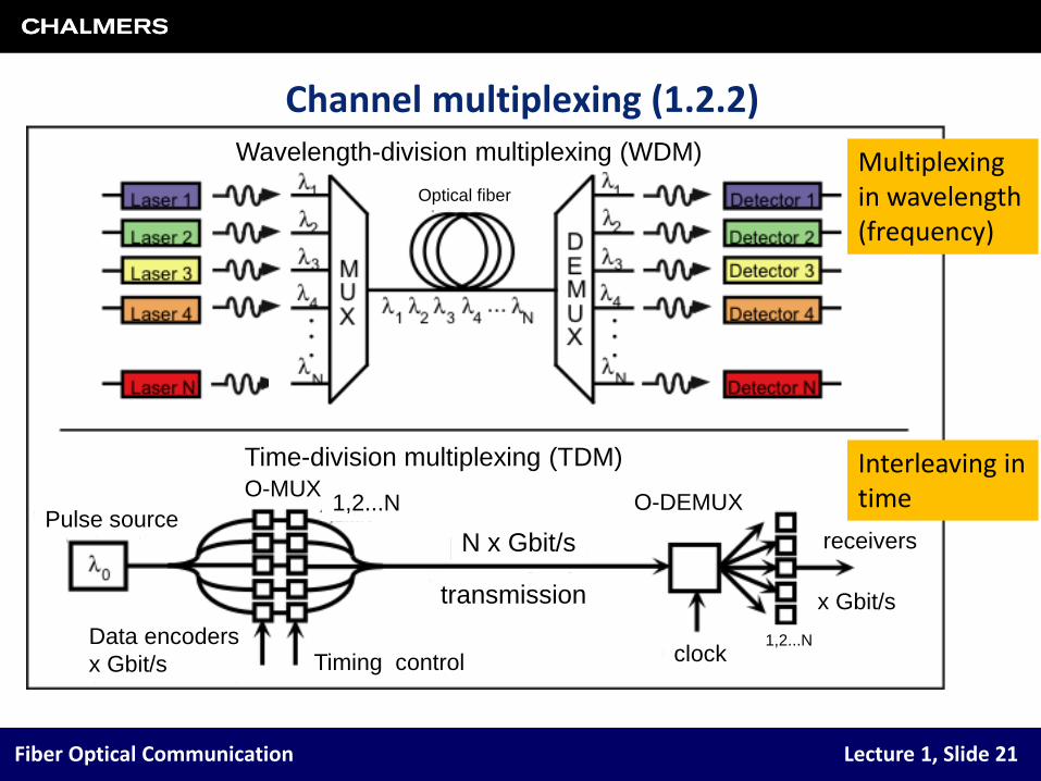
Channel multiplexing (1.2.2)Wavelength-division multiplexing (WDM)
Time-division multiplexing (TDM)
Optical fiber
Pulse source
O-MUX1,2...N
Data encoders
x Gbit/s Timing control clock1,2...N
receivers
x Gbit/s
O-DEMUX
N x Gbit/s
transmission
Multiplexing in wavelength (frequency)
Interleaving in time
Fiber Optical Communication Lecture 1, Slide 22
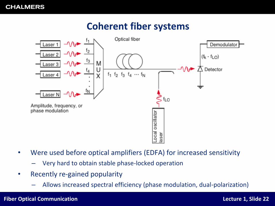
Coherent fiber systems
• Were used before optical amplifiers (EDFA) for increased sensitivity
– Very hard to obtain stable phase-locked operation
• Recently re-gained popularity
– Allows increased spectral efficiency (phase modulation, dual-polarization)

Fiber Optical Communication Lecture 1, Slide 23
The dB units (1.4.2)• Decibel (dB) expresses a power ratio according to
• The photo current is proportional to the optical power
– Idet Popt ⇒ Pel Popt2
– dBopt ≠ dBel (3 dB optical power diff. ⇒ 6 dB electrical power diff.)
• dBm expresses the absolute power on a log scale relative to 1 mW
• Examples:
– 1 mW = 0 dBm, 2 mW = 3 dBm, 4 mW = 6 dBm, 8 mW = 9 dBm
– 0.5 mW = –3 dBm, 1 μW = –30 dBm
– 100 mW = 20 dBm, 400 mW = 26 dBm
2
110log10
P
P
mW1
W][log10 10dBm
PP

Fiber Optical Communication Lecture 1, Slide 24
Optical fibers (2.1)Typical core sizes:
• Single-mode fibers: d ≈ 5–10 µm
• Multi-mode fibers: d ≈ 50–200 µm
• Typical attenuation:
– 0.2 dB/[email protected] µm
– 4% power loss per [email protected] µm
• Available bandwidth:
– >30 THz in modern fibers
1.3 1.55Wavelength (µm)
Att
enuat
ion (
dB
/km
)0.2
15 THz 20 THz
n1 > n2
cladding, n2
core, n1d

Fiber Optical Communication Lecture 1, Slide 25
Fiber basics• Wave-guiding: n1 > n2
• A finite number of modes can propagate in the fiber
• Modes are solutions to Maxwell's equations + boundary conditions
– One mode: single-mode fiber
– Several modes: multi-mode fiber
• Most commonly used fiber material is silica (SiO2)
• To change index of refraction dopants are added
– Dopants can increase or decrease the index of refraction
– Can dope either the core or the cladding
core cladding protective coating
2a2b
n1 n2
refr
active
ind
ex
dopant addition [mol %]
1.44
1.46
1.48
5 10 15 200
F
GeO2
B2O3

Fiber Optical Communication Lecture 1, Slide 26
Geometrical-optics description• The fractional index change is
– Δ ≈ 1–3% for MM fibers
– Δ ≈ 0.1–1% for SM fibers
– n2 = n1(1 – Δ)
• Apply Snell's law at input
• Minimum critical angle φc for total internal reflection
• Relate to maximum entrance angle
cladding, n2
core, n1
unguided ray
ir guided ray
n0(normally = 1)
1/)( 121 nnn
ri nn sinsin 10
1221 /sin)2/sin(sin nnnn cc
2
2
2
1
2
111max,1max,0 sin1cos)2/sin(sinsin nnnnnnn cccri

Fiber Optical Communication Lecture 1, Slide 27
Numerical aperture• The numerical aperture (NA) is a measure of the light-gathering power of
an optical system
– The term originates from microscopy
• For fibers, we have
• Clearly, a higher NA is always better!?!
– No, we get problems with dispersion
cladding, n2
core, n1
unguided ray
ir guided ray
n0(normally = 1)
2sinNA 1
2
2
2
1max,0 nnnn i

Fiber Optical Communication Lecture 1, Slide 28
• Compare the propagation times along the slowest and the fastest path
• For this approximate model, use the condition TB = 1/B > ΔT
– Means: Propagation time difference < bit slot
• We get a limit on the bit rate-distance product
– Do not confuse ΔT with Δ
Modal dispersion (multi-mode fiber)
cladding, n2
core, n1
i,max
c
fastest ray path
slowest ray path
2
2
11
2
11
1
fastslow 1sin/ n
n
c
L
c
n
n
nL
c
nL
L
nc
LLT
c
c
n
nBL
2
1
2
Fiber Optical Communication Lecture 1, Slide 29
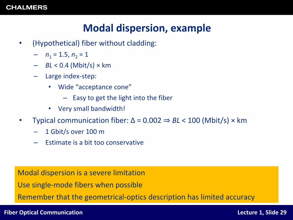
Modal dispersion, example
Modal dispersion is a severe limitation
Use single-mode fibers when possible
Remember that the geometrical-optics description has limited accuracy
• (Hypothetical) fiber without cladding:
– n1 = 1.5, n2 = 1
– BL < 0.4 (Mbit/s) × km
– Large index-step:
• Wide “acceptance cone”
– Easy to get the light into the fiber
• Very small bandwidth!
• Typical communication fiber: Δ = 0.002 ⇒ BL < 100 (Mbit/s) × km
– 1 Gbit/s over 100 m
– Estimate is a bit too conservative

Fiber Optical Communication Lecture 1, Slide 30
Basic fiber typesSingle-mode step-index:
• No intermodal dispersion gives highest bandwidth
• Small core radius, difficult to launch light
Multi-mode step-index:
• Large core radius, easy to launch light
• Intermodal dispersion reduces the bandwidth
Multi-mode graded-index:
• Reduced intermodal dispersion increases bandwidth
n
2a: 5-12 m
2b: 125 m
n
a b
n2
n1
2a: 50-200 m
2b: 125-400 m
n
2a: 50-100 m
2b: 125-140 m

Fiber Optical Communication Lecture 1, Slide 31
Other types of fiberPolarization preserving fibers
• Using birefringence
Photonic crystal fibers
• Air capillaries inside fiber

Fiber Optical Communication Lecture 1, Slide 32
Fiber fabrication (2.7)• Preform is made from glass (2–20 cm thick cylinder)
• Heated and pulled to 125 µm diameter
• Adding coating for mechanical protection

Fiber Optical Communication Lecture 1, Slide 33
A 2 inch wafer with optical components

Fiber Optical Communication Lecture 1, Slide 34
Optical modulator (LiNbO3)

Fiber Optical Communication Lecture 1, Slide 35
A complete transponder