A definition of Fiber Optics - ttu.ee 11.pdf · Fiber Optical Communication Lecture 11, Slide 5...

Fiber Optical Communication Lecture 11, Slide 1

Lecture 11

• Noise from optical amplifiers

– EDFA noise

– Raman noise

• Optical SNR (OSNR), noise figure, (electrical) SNR

• Amplifier and receiver noise

– ASE and shot/thermal noise

• Preamplification for SNR improvement


Amplifier noise• All amplifiers add noise

– To amplify (make a larger copy), a physical device must ”observe” the signal

– Cannot be done without perturbing the signal

• Assured by the Heisenberg uncertainty principle

• Lumped and distributed amplification have different performance

• Noise comes from spontaneously emitted photons

• These have random

– direction

– polarization

– frequency (within the band)

– phase

• Some of these add to the signal

– Causes intensity and phase noise


• Optical signals are often characterized by the optical SNR (OSNR)

– Easily measured with an optical spectrum analyzer (OSA)

• Makes signal monitoring in the lab easy ⇒ is very popular

• The definition of the OSNR is

– The index X and Y denote the two polarizations

• The OSNR is related to the SNR, Q, and BER

• OSNR is usually normalized to a 0.1 nm bandwidth

– Entire signal power is included, noise is measured over 0.1 nm

– Implies required OSNR (for given BER) is bit rate-dependent

Definition of the optical SNR

OSNR

ASE

signal

Ynoise,Xnoise,

Ysignal,Xsignal,

2}signalonpolarizatisingleFor{OSNR

P

P

PP

PP


EDFA noise (7.2.3)• The noise is called amplified spontaneous emission (ASE)

– Is being amplified since there is gain

– Will reach the receiver (remaining optical path is amplified)

• The ASE power at the output of the EDFA

– Δν0 is the effective bandwidth of the optical filter used to suppress noise

– SASE is the (onesided) noise power spectral density (PSD)

– This is the power per polarization

• nsp is the spontaneous-emission factor also known as the population-inversion factor

– For an EDFA

oo GhnSP )1(0spASEASE

112

2

12

2sp

NN

N

NN

Nn

a

s

e

s

e

s


OSNR due to EDFA noise (7.4.1)• The OSNR is reduced each time a signal is amplified

– Each EDFA add to the noise PSD due to the generation of more ASE

• After NA amplifiers in a link with span loss equal to the gain in each amplifier and with identical EDFA noise performance, we have

• In dB and dBm at 1550 nm and Δν0 = 0.1 nm, we have

Ps

EDFALA

1 2 NAPs

dBm58dB][dB][2dB][dBm][OSNR spindB GnNP A

GhnN

P

GhnN

P

PN

P

oAooAA 1.0sp

in

sp

in

ASE

in

2)1(22OSNR


What is the max. transmission distance with 100 km or 50 km EDFA spacing?

– A 10 Gbit/s system with a OSNR requirement of 20 dB

– The loss is 0.25 dB/km and 2nsp = 5 dB

– The launched power into each span is 1 mW per WDM channel

– LA = 100 km ⇒ NA = 8 dB = 6.3 ⇒ 6 amps ⇒ 700 km

– LA = 50 km ⇒ NA= 20.5 dB = 112.2 ⇒ 112 amps ⇒ 5650 km

• The amplifier spacing plays a critical role for the OSNR

– Short LA: Noise accumulates slowly ⇒ high OSNR at receiver

– Long LA: Few EDFAs are needed ⇒ system cost is lower

• Shows trade-off between cost and performance

– Techniques that enable cost reduction are desirable

• This can, for example, be error correction or distributed amplification

• Hints that distributed amplification may perform better

OSNR due to EDFA noise, example

dBm58dB][dB][2dB][dBm][OSNR spindB GnNP A


OSNR due to EDFA noise, amplifier spacing• We can express the number of amplifiers as

– LT is the total system length

– This gives the OSNR

• We see that

• Figure shows maximum system length = ”system reach”

– OSNR = 20 dB

– α = 0.2 dB/km

– nsp =1.6

– Δν0 = 100 GHz

G

LN T

Aln

)1(2

lnOSNR

1.00sp

in

GLhn

GP

T

G

GP

ln

1ASE


Raman amplifier noise (7.3.4)• Noise is generated by spontaneous Raman scattering

• The noise PSD per polarization after an amplified fiber is

– Depends on the net power gain, G(L)

• Observe: This is net gain, for a transparent system G(L) = 1

– Depends on the distribution of gain g0(z)

• nsp has a different definition for Raman amplification

– h is Planck’s constant

– νR is the Raman shift

• Maximum gain at 13.2 THz

– kB is Boltzmann’s constant

– T is the temperature, ≈ 293 K

• This gives nsp = 1.13, nsp → 1 as T → 0

L

dzzG

zgLGhnS

0

00spASE

)(

)()(

p

pR

a

zPgzg

)()(0

z

s dgzG0

0 ])([exp)(

)/exp(1

1sp

Tkhn

BR


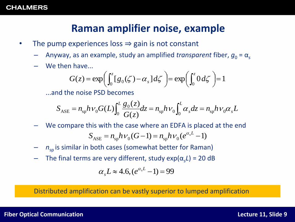
Raman amplifier noise, example• The pump experiences loss ⇒ gain is not constant

– Anyway, as an example, study an amplified transparent fiber, g0 = αs

– We then have...

...and the noise PSD becomes

– We compare this with the case where an EDFA is placed at the end

– nsp is similar in both cases (somewhat better for Raman)

– The final terms are very different, study exp(αsL) = 20 dB

10exp])([exp)(00

0

zz

s ddgzG

LhndzhndzzG

zgLGhnS s

L

s

L

0sp0

0sp0

00spASE

)(

)()(

)1()1( 0sp0spASE LsehnGhnS

99)1(,6.4 L

sseL

Distributed amplification can be vastly superior to lumped amplification


OSNR due to Raman noise (7.4.2)• Pump stations are set up spaced by LA

– Gain is designed to make Ps(z = nLA) = Pin

• The OSNR is given by

– SASE must be found using the general expression

– Depends on pumping; forward, backward, or both

• Figure shows ASE PSD and OSNR, fiber is 100 km long

– Pumping is bidirectional to varying degree

– System is transparent at 0 dB net gain

– Forward pumping is better than backward pumping

• Nonlinearities are not considered

1.0ASE

in

2OSNR

SN

P

A


Raman amplifier performance• In general, it is preferable to amplify a strong signal

– For a given gain (and added noise PSD), the (O)SNR decrease is smaller

– Forward pumping is better than backward pumping

– Unfortunately, signal power must be limited due to nonlinearities

• The Raman amplifier is affected by several phenomena:

– Double Rayleigh scattering occurs

• Light scattered back is scattered again

– Pump-noise transfer decreases the SNR

• The gain changes with the pump intensity fluctuations

– The amplifier is polarization dependent

• Is counteracted using polarization scrambling


Electrical signal-to-noise ratio (SNR) (7.5.1)• The Q and BER are determined by the SNR in the detected current

– Agrawal calls this ”electrical signal-to-noise ratio” to separate from OSNR

• An EDFA can improve the sensitivity of a thermally noise limited receiver

– A preamplified optical receiver

– The added optical noise can be much smaller than the thermal noise

• The generated photocurrent in the receiver is

– Ecp = ASE co-polarized with signal

– Eop = ASE orthogonal with signal

– is = Shot noise

– iT = Thermal noise

• The ASE has a broad spectrum, and can be written

– The magnitude square is a multiplication ⇒ new frequenciesare generated ⇒ “beating”

Gnsp

PinBPF

receiver

Tssd iiEEEGRI

2

op

2

cp

M

m

mms tiiSE1

2/1

ASEcp )exp()(


Electrical signal-to-noise ratio (SNR)• The received electrical current is

– isig-sp = signal-ASE beat noise term

– isp-sp = ASE-ASE beat noise term

• The variance of the noise terms are

– Δν0 is bandwidth of optical bandpass filter (rejects out-of-band noise)

• The SNR is here defined as

Tssd iiiiGPRI spspspsig

fSGPR sd ASE

22

spsig 4 )2/(4 0

2

ASE

22

spsp ffSRd

fPGPRq sds )(2 ASE

2 fRTk LBT )/4(2

222

spsp

2

spsig

2

2

2

)(SNR

Ts

sdGPRI


Impact of ASE on SNR (7.5.2)• Let us compare the SNR without and with amplification by an EDFA

– Amplifier and bandpass filter is inserted before the receiver

– Notice that σs are different in the two cases (σT stays the same)

– We neglect σsp-sp and the noise current contribution to shot noise to get

– We use the PSD and the ideal responsivity

– We get

• Notice: kT is ratio (thermal noise)/(shot noise) without amplification

• All quantities in the denominator (2qRdPsΔf) are kept constant!

222

spsp

2

spsig

2

amp22

2

amp no

)(SNR,

)(SNR

Ts

sd

Ts

sd GPRPR

2

2

2

ASE

2

2

amp no

amp

)(

)2(

)2()4(

)(

SNR

SNR

sd

Tsd

Tsdsd

sd

PR

fPqR

fGPqRfSGPR

GPR

GhnGGhnS 0sp0spASE }1{)1( )/( 0hqRd

2

spamp no

amp

//12

1

SNR

SNR

GkGn

k

T

T

fPqRk

sd

TT

2

2


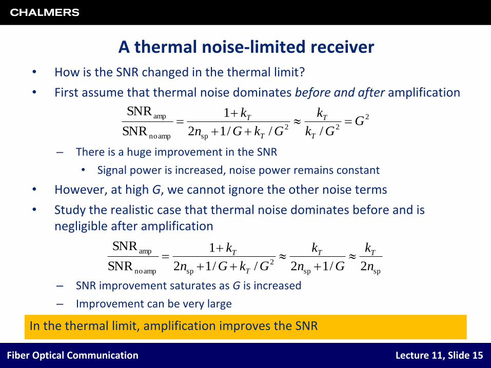
A thermal noise-limited receiver• How is the SNR changed in the thermal limit?

• First assume that thermal noise dominates before and after amplification

– There is a huge improvement in the SNR

• Signal power is increased, noise power remains constant

• However, at high G, we cannot ignore the other noise terms

• Study the realistic case that thermal noise dominates before and is negligible after amplification

– SNR improvement saturates as G is increased

– Improvement can be very large

2

22

spamp no

amp

///12

1

SNR

SNRG

Gk

k

GkGn

k

T

T

T

T

spsp

2

spamp no

amp

2/12//12

1

SNR

SNR

n

k

Gn

k

GkGn

k TT

T

T

In the thermal limit, amplification improves the SNR


A shot noise-limited receiver, noise figure (7.2.3)• Now instead assume that the optical signal has high power

– Thermal noise is negligible

– The SNR is decreased by the amplification

• The noise figure is defined

• The SNR values are what you would obtain by putting an ideal receiver before and after an EDFA, respectively

– Ideal means shot noise-limited, 100% quantum efficiency

• Our study above has provided us with the (inverse) minimum value

spsp

2

spamp no

amp

2

1

/12

1

//12

1

SNR

SNR

nGnGkGn

k

T

T

EDFA amplification of a perfect signal decreases the SNR by > 2nsp (> 3dB)

out

in

)SNR(

)SNR(NF nF

22 sp nFn


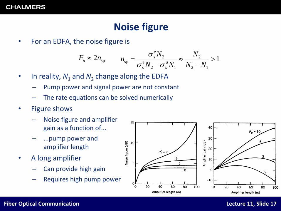
Noise figure• For an EDFA, the noise figure is

• In reality, N1 and N2 change along the EDFA

– Pump power and signal power are not constant

– The rate equations can be solved numerically

• Figure shows

– Noise figure and amplifier gain as a function of...

– ...pump power and amplifier length

• A long amplifier

– Can provide high gain

– Requires high pump power

sp2nFn 112

2

12

2sp

NN

N

NN

Nn

a

s

e

s

e

s


Noise figure• The noise figure is increased

– If the population inversion is incomplete (somewhere in the amplifier)

– If there are coupling losses into the amplifier

• Pumping is facilitated by pumping at 980 nm

– No stimulated emission caused by pump photons (σpe ≈ 0)

• Corresponding energy level is almost empty (short-lived)

– Noise figure ≈ 3 dB is possible, 3.2 dB has been measured

• With 1480 nm pumping σpe ≠ 0

– Ground state will always be populated by some ions

• Some excited ions will be stimulated by pump photons to relax

– Noise figure is larger for this case

• Coupling into and out of an EDFA is efficient

• Typical EDFA modules have Fn = 4–6 dB


SNR/OSNR relation• In general, there is no simple relation between the OSNR and the SNR

– OSNR is prop. to the optical power, SNR is prop. to the electrical power

– Electrical power is proportional to the (optical power)2

• Not true in a coherent receiver

• When signal–ASE noise is dominating we have

• For a single-polarization signal, we can use

– Es is the energy per symbol, fs is the symbol rate (in baud)

– Es/SASE is often written Es/N0 is digital communication literature

– The relation between Es/N0 and the BER depends on the type of receiver, modulation format and more

OSNR244

)(SNR 1.0

ASE

1.0

ASE

2

2

ffP

GP

fSGPR

GPR s

sd

sd

1.0ASE1.0ASE 22OSNR

sss f

S

E

S

P


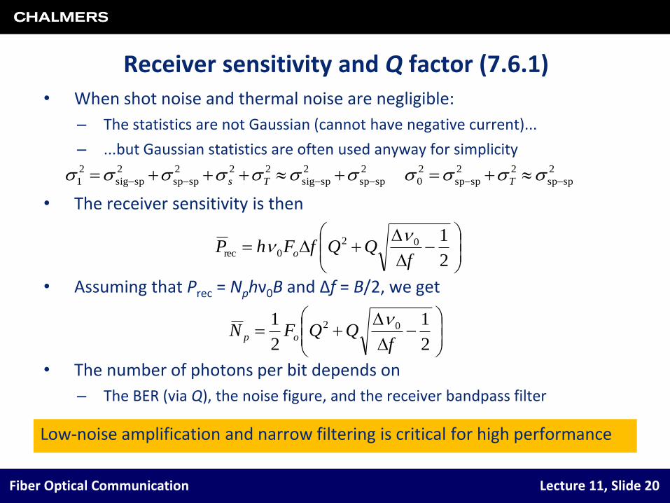
Receiver sensitivity and Q factor (7.6.1)• When shot noise and thermal noise are negligible:

– The statistics are not Gaussian (cannot have negative current)...

– ...but Gaussian statistics are often used anyway for simplicity

• The receiver sensitivity is then

• Assuming that Prec = Nphν0B and Δf = B/2, we get

• The number of photons per bit depends on

– The BER (via Q), the noise figure, and the receiver bandpass filter

2

spsp

2

spsig

222

spsp

2

spsig

2

1 Ts

2

spsp

22

spsp

2

0 T

2

102

0recf

QQfFhP o

2

1

2

1 02

fQQFN op

Low-noise amplification and narrow filtering is critical for high performance


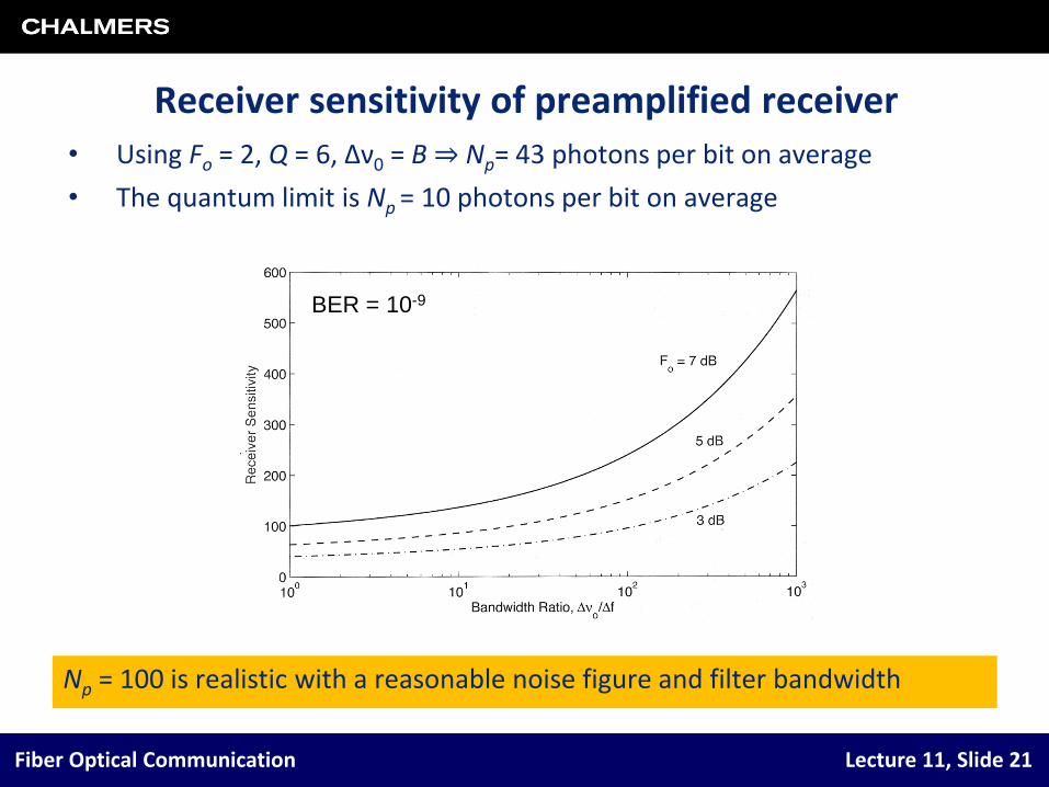
Receiver sensitivity of preamplified receiver• Using Fo = 2, Q = 6, Δν0 = B⇒ Np= 43 photons per bit on average

• The quantum limit is Np = 10 photons per bit on average

BER = 10-9

Np = 100 is realistic with a reasonable noise figure and filter bandwidth


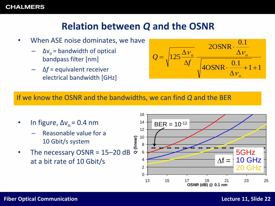
Relation between Q and the OSNR• When ASE noise dominates, we have

– Δνo = bandwidth of optical bandpass filter [nm]

– Δf = equivalent receiver electrical bandwidth [GHz]

• In figure, Δνo = 0.4 nm

– Reasonable value for a 10 Gbit/s system

• The necessary OSNR = 15–20 dBat a bit rate of 10 Gbit/s

111.0

OSNR4

1.0OSNR2

125

o

oo

fQ

0

2

4

6

8

10

12

14

16

13 15 17 19 21 23 25OSNR (dB) @ 0.1 nm

Q (

lin

ear)

f =5GHz10 GHz20 GHz

BER = 10-12

If we know the OSNR and the bandwidths, we can find Q and the BER


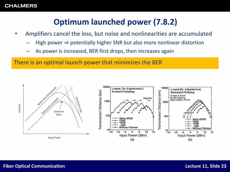
Optimum launched power (7.8.2)• Amplifiers cancel the loss, but noise and nonlinearities are accumulated

– High power ⇒ potentially higher SNR but also more nonlinear distortion

– As power is increased, BER first drops, then increases again

There is an optimal launch power that minimizes the BER

A definition of Fiber Optics - ttu.ee 11.pdf · Fiber Optical Communication Lecture 11, Slide 5...

Documents

Transcript of A definition of Fiber Optics - ttu.ee 11.pdf · Fiber Optical Communication Lecture 11, Slide 5...