TECHNICAL REPORT 0-90-1

ANALYSIS OF WIDEBAND BEAMFORMERSDESIGNED WITH ARTIFICIAL NEURAL NETWORKS

by

Cary Cox

Instrumentation Services Division

DEPARTMENT OF THE ARMY00 Waterways Experiment Station, Corps of Engineersco 3909 Halls Ferry Road, Vicksburg, Mississippi 39180-6199

" ~ jCa.*

FEE 0O6 9i1

OUTPUTST)

OUTPUTS

OUTPUTS 'f)

December 1990Final Report

Approved for Public Release; Distribution Unlimited

c Prepared for DEPARTMENT OF THE ARMYAssistant Secretary of the Army (R&D)

Washington, DC 20315

Under Work No. A91 D-LR-006

0j 06 042

Destroy this report when no longer needed. Do not returnit to the originator.

(

The findings in this report are not to be construed as an officialDepartment of the Army position unless so designated

by other authorized documents.

The contents of this report are not to be used foradvertising, publication, or promotional purposes.Citation of trade names does not constitute anofficial endorsement or approval of the use of

such commercial products.

Form ApprovedREPORT DOCUMENTATION PAGE [ OMB No. 0704-0188

Pubic reporrrr burden for this ollectlon of nformaton ,s estnated to aleraqe 1 hour Der resOc,'se, iluding the trme tot reviewinq instructiOns. Searc inq existlng data sourcesgathfernq and marnta'nng the data needed. and comoletlnq and reviewnq the (ollection of information Send comments regarding this Ourden estnimate or anV other aspect of thiscOlol'rtion of informat on. ncludn suggeittons for reducing thns Ourden to Vashnqton Headuarterl Services. Directorate for information Operations and Report$, 12 15 JeffersonOa qfwa . uite 1204. A ington. 4A 22202-4302, and to the Office of Management and Budget. Paperwork Reduction Project (0704-0188). Washington DC 20503

1. AGENCY USE ONLY (Leave blank) 2. REPORT DATE T3. REPORT TYPE AND DATES COVEREDDecember 1990 Final report

4. TITLE AND SUBTITLE 5. FUNDING NUMBERS

Analysis of Wideband Beamformers Designed with Artificial NeuralNetworks

6. AUTHOR(S)

Cary Cox

7. PERFORMING ORGANIZATION NAME(S) AND ADDRESS(ES) 8. PERFORMING ORGANIZATION

REPORT NUMBER

USAE Waterways Experiment StationInstrumentation Services Division Technical Report 0-90-13909 Halls Ferry RoadVicksburg, MS 39180-6199

9. SPONSORING / MONITORING AGENCY NAME(S) AND ADDRESS(ES) 10. SPONSORING/ MONITORINGAGENCY REP,,ST NUMBER

Assistant Secretary of the Army

Washington, DC 20315

11. SUPPLEMENTARY NOTES

Available from National Technical Information Service, 5285 Port Royal Road, Springfield, VA 22161

12a. DISTRIBUTION fAVAILABILITY STATEMENT 12b. DISTRIBUTION CODE

Approved for public release; distribution unlimited

13. ABSTRACT (Maximum2Onworcas)

The ability Lo determine the direction of an approaching wave is demonstrated by using an artificialneural network and a beamformer array. To demonstrate the ability of a neural network to learn a satisfac-tory solution to this problem, simulations were performed to test the system's sensitivity to several variables.These variables include amplitude range, noise level, frequency bandwidth, linear and nonlinear inputs, thenumber of sensor inputs, and the number of hidden units used in the network. Simulations are provided forboth narrowband and wideband signals. An empirical test and a comparison between ANN beamformers andFFT beamformers are also used to demonstrate the strengths and weaknesses of the system. A design ex-ample and a description of the simulation program are also included. A briel tutorial on beamformers andneural networks is also provided.

14. SUBJECT TERMS 15, NUMBER OF PAGESArtificial neural networks Fecdforwa:,l rietworks 244Backpropag- z'cz Direction of arrival 16. PRICE CODEBeam formers

17. SECURITY CLASSIFICATION 18. SECURITY CLASSIFICATION 19. SECURITY CLASSIFICATION 20. LIMITATION OF ABSTRACTOF REPORT OF THIS PAGE OF ABSTRACT

UNCLASSIFIED UNCLASSIFIED INSN 7540-01-280-5500 Sandard Form 298 (Rev 2-89)

P,"-red bv ANSI Std 139.18

298-102

PREFACE

This investigation was performed by personnel of the US

Army Engineer Waterways Experiment Station (WES) under the

In-House Laboratory Independent Research Program (ILIR). The

work was performed under Work Number A91D-LR-006, "Analysis

of Wideband Beamformers Designed with Artificial Neural

Networks".

The study was conducted under the general supervision of

Messrs. George P. Bonner, Chief, Instrumentation Services

Division and Leiland M. Duke, Chief, Operations Branch. This

report was written by Dr. Cary B. Cox, Data Reduction and

Digital Support Section, Instrumentation Services Division.

This study was also published as a dissertation for Mississippi

State University under the direction of Dr. F. M. Ingels of

the Electrical Engineering Department.

The Commander and Director of WES during preparation of

this report was COL Larry B. Fulton. Technical Director was

Dr. Robert W. Whalin.A',2-Ion For

II r, -q . . ./' I~- C ) ' \.

A'.. ... .. .

1Ii tt

Table of Contents

List of Figures......................................... Vi

List of Tables........................................... x

Chapter 1 Introduction................................... 11.1 Artificial Neural Networks........................i11.2 Beamformer Arrays................................. 51.3 Purpose of Dissertation........................... 61.4 Outline of Dissertation........................... 8

Chapter 2 Tutorial On Artificial Neural Networks ....... 132.1 Artificial Neuron Models......................... 13

2.1.1 Adaptive Linear Element..................... 132.1.2 Perceptrons................................. 152.1.3 Backpropagation Perceptrons .................15

2.2 Types of Artificial Neural Networks ..............212.2.1 Feedforward Networks........................ 222.2.2 Recurrent Networks.......................... 242.2.3 Bi-directional Associative Memory .......... 262.2.4 Adaptive Resonance Theory ...................27

2.3 Training......................................... 282.3.1 The Delta Rule.............................. 292.3.2 Backpropagation............................. 302.3.3 Statistical Training........................ 37

2.4 Linearly Separable Regions....................... 38

Chapter 3 Beamformer Fundamentals....................... 413.1 Basic Types of Beamformers....................... 413.2 Narrowband Beamformer............................ 413.3 Wideband Beamformers............................. 453.4 Previous Work.................................... 47

3.4.1 Fast Fourier Transform Wideband Beamformer.473.4.2 Adaptive Beamformers with ADALINES ......... 533.4.3 Beamforming with Hopfield Networks ......... 54

Chapter 4 Model of Narrowband Beamformer ................614.1 Beamformer Array Processing with ANN's .......... 614.2 Design of Narrowband Beamforner ..................624.3 Mathematical Analysis of Beamformer ............. 644.4 Results of Mathematically Designed Beamforner. ...694.5 Delta Rule Training of Narrowband Beamfornier .... 744.6 Results '-f Tr'P'ing with the DQ~ta Rule ......... 75

4.7 Backpropagation Training of Beamformer .......... 774.8 Results of Training with Backpropagation ........ 824.9 Narrowband Beamformers with Nonlinear Inputs .... 944.10 Results of Beamformer with Nonlinear Inputs .... 964.11 The Network's Dependency on Time ............... 97

Chapter 5 Model of Wideband Beamformer ................ 1095.1 Design of Wideband Beawformer .................. 1095.2 Mathematical Analysis of Wideband Beamformer... 1095.3 Wideband Beamformers Using Backpropagation ..... 1125.4 Results of Beamformers Trained with

Backpropagation ................................. 112

Chapter 6 Empirical Demonstration and Comparison ofFFT and ANN Beamformers ..................... 126

6.1 Seismic Test Description ....................... 1266.2 Results of Seismic Test ........................ 1296.3 Comparisons between FFT Beamformers and

ANN Beamformers ................................ 1386.3.1 Simulation Comparisons of FFT and

Beamformers ................................ 1406.3.2 Results of the Comparison of ANN and

FFT Beamformers ........................... 1546.3.3 Processing Requirements for FFT and

ANN Beamformers ........................... 1556.3.4 Summary of FFT and ANN Beamformer

Comparison ................................. 157

Chapter 7 Proposed Design Criteria .................... 1617.1 Summary of Beamformer Design Criteria .......... 1617.2 Description of Simulation Program .............. 1657.3 Examples of Beamformer Design .................. 168

Chapter 8 Survey of ANN Hardware ...................... 1728.1 Artificial Neural Network Hardware ............. 1728.2 ANN Integrated Circuits ........................ 173

8.2.1 Available Integrated Circuits ............. 1758.3 Artificial Neural Network Computers ............ 1778.4 Best ANN Options for Feedforward Networks ...... 180

Chapter 9 Conclusions and Recommendations ............. 1829.1 Conclusions ..................................... 1829.2 Recommendations................................ 183

References ............................................ 186

iv

Appendix I Wideband Beamformer Simulation Program ..... 189

Appendix II Time History Plots of Seismic Data ....... 222

v

List of Figures

Figure 1 Biological Neurons ............................. 3Figure 2 Ideal Response of an ANN Beamformer ........... 12Figure 3 Diagram of ADALINE ............................ 14Figure 4 Model of Perceptron ........................... 15Figure 5 Backpropagation Perceptron .................... 16Figure 6 Multilevel ANN ................................. 17Figure 7 Fully Connected Neural Network ................ 23Figure 8 Recurrent Network .............................. 25Figure 9 Model of BAM ................................... 27Figure 10 Error Curve ................................... 31Figure 11 Error Curve with Local Minima ................ 36Figure 12 Example of Linearly Separable Region ......... 39Figure 13 Beamformer Array ............................. 42Figure 14 Wideband Beamformer .......................... 46Figure 15 DFT Narrowband Beamformer Response ........... 51Figure 16 DFT Wideband Beamformer Response ............. 52Figure 17 Hopfield Network for Beamforming ............. 54Figure 18 Angle Response of Hopfield Net ANN ........... 59Figure 19 Hopfield Network Detection of 3 Angles ...... 60Figure 20 Graph of 2 Signal System ..................... 63Figure 21 Segmented Network ............................ 64Figure 22 Mathmatically Designed Response .............. 68Figure 23 Mathmatical Designed ANN Using 2

Hidden Units .................................. 71Figure 24 Mathmatically Designed ANN Using 3

Hidden Units .................................. 72Figure 25 Mathmatically Designed ANN Using 20

Hidden Units ................................. 73Figure 26 Narrowband Beamformer for One Arrival

Angle ........................................ 74Figure 27 Delta Rule Trained ANN with 2

Hidden Units .................................. 78Figure 28 Delta Rule Trained ANN with 3

Hidden Units ................................. 79Figure 29 Delta Rule Trained ANN with 20

Hidden Units .................................. 80Figure 30 Narrowband Beamformer ........................ 81Figure 31 Average Output of Backpropagation ANN

with 2 Hidden Units .......................... 84Figure 32 Average Output of Backpropagation ANN

with 3 Hidden Units .......................... 85

vi

Figure 33 Average Output of Backpropagation ANNwith 20 Hidden Units ......................... 86

Figure 34 ANN with 2 Hidden Units and AmplitudeRange of .5-2 ................................ 88

Figure 35 ANN with 3 Hidden Units and AmplitudeRange of .5-2 ................................ 89

Figure 36 ANN with 20 Hidden Units and AmplitudeRange of .5-2 ................................ 90

Figure 37 ANN with 2 Hidden Units and Noise of .2 .... 91Figure 38 ANN with 3 Hidden Units and Noise of .4 .... 92Figure 39 ANN with 20 Hidden Units and Noise of .8 .... 93Figure 40 Separation of Angles ......................... 95Figure 41 Separation of Angles and Amplitudes .......... 96Figure 42 Exact Simulation; I0 Inputs;

Amplitude Range .5-1.0 ....................... 99Figure 43 Exact Simulation; 20 Inputs;

Amplitude Range .5-1 ........................ 100Figure 44 Exact Simulation; 10 Inputs;

Amplitude Range .5-2 ........................ 101Figure 45 Exact Simulation; 20 Inputs;

Amplitude Range .5-2 ........................ 102Figure 46 Elliptical Simulation; 10 Inputs;

Amplitude Range of .5-1 ..................... 103Figure 47 Elliptical Simulation, 20 Inputs;

Amplitude .5-1.0 ............................ 104Figure 48 Elliptical Simulation; 10 Inputs;

Amplitude Range of .5-2 ..................... 105Figure 49 Elliptical Simulation, 20 Inputs;

Amplitude Range .5-2 ........................ 106Figure 50 Simulation with Linear Inputs ............... 107Figure 51 Simulation with Nonlinear Inputs ............ 108Figure 52 Two Dimensional Beamformer ................... 110Figure 53 Linear Wideband ANN, 3x3 Hidden Units ....... 114Figure 54 Exact Wideband ANN, 3x3 Hidden Units ........ 115Figure 55 Elliptical Wideband ANN, 3x3 Hidden

Units ....................................... 116Figure 56 Linear Wideband ANN, 6x6 Hidden Units ....... 117Figure 57 Exact Wideband ANN, 6x6 Hidden Units ........ 118Figure 58 Elliptical Wideband ANN, 6x6 Hidden

Units ....................................... 119Figure 59 Linear Wideband ANN, 10xlO Hidden Units ..... 120Figure 60 Exact Wideband ANN, 10xl0 Hidden Units ...... 121Figure 61 Elliptical Wideband ANN, 10xl0 Hidden Units.122Figure 62 Linear Wideband ANN, 1 Frequency

Component ................................... 123

vii

Figure 63 Linear Wideband ANN, 2 FrequencyComponents .................................. 124

Figure 64 Linear Wideband ANN, 7 FrequencyComponents .................................. 125

Figure 65 Siesmic Test Diagram ........................ 127Figure 66 First Simulation with Training Data as

Input ....................................... 131Figure 67 First Simulation with Similar Data as

Input ....................................... 132Figure 68 First Simulation with Different Range

of Data as Input ............................ 133Figure 69 Second Simulation with Different Range

of Data as Input ............................ 134Figure 70 Simulation with Similar Data as Input ....... 135Figure 71 Simulation with Different Range of Data

as Input .................................... 136Figure 72 Narrowband DFT Beamformer; No Noise ......... 142Figure 73 Narrowband DFT Beamformer; Noise

Level 1.0 ................................... 143Figure 74 Narrowband ANN Beamformer; No Noise ......... 144Figure 75 Narrowband ANN Beamformer; Noise

Level 1.0 ................................... 145Figure 76 Wideband DFT Beamformer; 3 Sub-arrays;

No Noise .................................... 146Figure 77 Wideband DFT Beamformer; 3 Sub-arrays;

Noise Level 1.0 ............................. 147Figure 78 Wideband DFT Beamformer; 4 Sub-arrays;

No Noise .................................... 148Figure 79 Wideband DFT Beamformer; 4 Sub-arrays;

Noise Level 1.0 ............................. 149Figure 80 Wideband ANN BEamformer; 2 Arrays;

No Noise .................................... 150Figure 81 Wideband ANN Beamformer* 2 Arrays;

Noise Level 1.0 ............................. 151Figure 82 Wideband ANN Beamformer; 3 Arrays;

No Noise .................................... 152Figure 83 Wideband ANN Beamformer; 3 Arrays;

Noise Level 1.0 ............................. 153Figure 84 Number of Sensors Versus % Good ............. 163Figure 85 Number of Hidden Units Versus % Good ........ 163Figure 86 Amplitude Range Versus % Good ............... 164Figure 87 Frequency Range Versus % Good ............... 164Figure 88 Noise Level Versus % Good .................... 165Figure 89 Design Example Simulation with 10

Sensors ..................................... 169

viii

Figure 90 Design Example Simulation with 20Sensors...................................... 170

Figure 91 Design Example Simulation with 30Sensors...................................... 171

ix

List of Tables

Table 1 Bandwidth of Arrival Angles .................... 49Table 2 Comparison between Beamformers ................. 70Table 3 Comparison of Delta Rule Beamformer ............ 77Table 4 Comparison with Backpropagation

Beamformers .................................... 83Table 5 Comparison of Wideband Beamformer

Networks ...................................... 113Table 6 Percent Error in Seismic Test .................. 137Table 7 Comercially Available Neuro Computers ......... 178Table 8 Computer Execution Times ...................... 179

x

Chapter 1

Introduction

1.1 Artificial Neural Networks

Artificial Neural Networks (ANN) is a term used to describe

single or multilevel networks that use an artificial neuron

as the main processing element. These artificial neurons are

designed to emulate the functions performed by the biological

neurons found in the cerebral cortex. It is obvious to most

computer scientists that there are many classes of problems

that are extremely difficult to solve on a standard sequential

von Neumann computer but are very easy for the mammalian brain

to process. Pattern recognition is one example of these

problems. Programming a von Neumann computer to recognize

objects or patterns is very difficult and minor changes in the

object being recognized can easily cause the programs to fail.

The developing mind of a 2 year old child however can easily

recognize faces of parents, siblings, or hundreds of objects.

These recognitions can easily be made when distortions or

modifications such as changes in scale, rotation, or translation

1

2

occur. Even lower forms of animal life such as dogs and cats

can recognize sounds, objects, and smells.

In recent years an effort has been made to solve such

problems by emulating the functions of the cerebral cortex.

The cerebral cortex is composed of around 10 billion to 100

billion cells known as neurons. [14] These neurons are

connected in hierarchical networks with over 10,000 billion

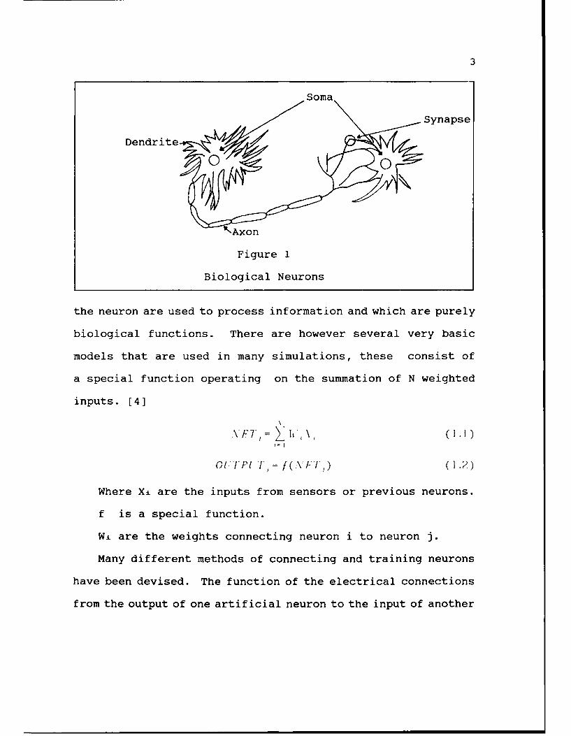
to 100,000 billion connections. A diagram of a biological

neuron is shown in Figure 1 [9]. There are four major parts

of the neuron.

(1) The "Soma" which is the main body of the neuron cell.

(2) An "Axon" which is attached to the soma and produces

an electrical pulse to be transmitted to other neurons.

(3) The "Dendrites" which receive these electrical signals.

(4) The "Synapses" which form the connections where two

dendrites meet.

In order to emulate these cells, mathematical models of

biological neurons have been devised. The sophistication of

these models ranges from very simple to extremely complex.

Detailed mathematical models of the biological neuron can be

very complex. Some researchers believe that these detailed

models should be used, while others believe that only the very

basic functions of the neuron should be included in a model.

This controversy can be partially explained by the uncertainty

that many neurologists have as to exactly which functions of

3

Synapse

Dendrite

Figure 1

Biological Neurons

the neuron are used to process information and which are purely

biological functions. There are however several very basic

models that are used in many simulations, these consist of

a special function operating on the summation of N weighted

inputs. [4]

V\FT,= \ (IIt)

Ol.( T 1 -,=f(..\ l,) (1.2)

Where X, are the inputs from sensors or previous neurons.

f is a special function.

Wi are the weights connecting neuron i to neuron j.

Many different methods of connecting and training neurons

have been devised. The function of the electrical connections

from the output of one artificial neuron to the input of another

4

artificial neuron (Xi) is analogous to the function of the

synapses that connect biological neurons to one another. The

strength of the connection that the synapse has with the neuron

influences the ability of the neuron to respond. The strength

of these synapses is analogous to the weights (Wi) in the

numerical model and the values assigned to these weights

determine the function the artificial neuron will perform.

One of the important characteristics of ANNs is that they

can be trained instead of programmed. Training can be

accomplished in a variety of ways. Weights can be preset based

on a numerical analysis of the problem and the network's

configuration or they can be taught acceptable values. This

teaching process is an iterative process performed by presenting

the inputs to the network with a set of patterns to be recognized

and adjusting weights in order to provide the desired output

response. This later method is of great importance in neural

network design since a formal mathematical analysis of many

problems can be extremely difficult.

An impressive amount of research which utilizes ANNs is

currently being conducted. There is an expectation that

integrated circuits can be designed which implement ANNs

using large scale integration. By designing dense ANN circuits

a large number of problems such as pattern recognition, verbal

word distinction, robotic controls, and signal processing may

be solved.

5

1.2 Beamformer Arrays

A beamformer array is an array of sensors that is used to

process signals in which direction is an important variable.

In some applications, in which the direction of thre source

of a signal is known, a beamformer array can be steered to

pickup the desired signal and filter out the noise being

transmitted from other directions. Another important

application is one in which the direction from which the

information being transmitted is not known. In this case the

direction can be determined by analyzing the data received

by the array. Several different methods of determining the

direction of a wavefront can be employed. If the signal being

transmitted has a narrow bandwidth, analog or digital techniques

can be used to analyze the array's output. From this analysis

the direction of the wavefront can be determined. However

when the signal being transmitted is composed of a wideband

of frequencies more complex methods must be employed to filter

the information in time in order to process only narrow bands

of frequencies. The processing of this information from

wideband beamformers can require the use of many filters and

operational amplifiers or a substantial digital signal

processing effort in order to discern the direction of the

wave.

6

1.3 Purpose of Dissertation

The purpose of this dissertation is to design and analyze

methods of determining the direction of arrival of a wideband

waveform using a beamformer array and an artificial neural

network. Recent research with neural networks has demonstrated

their ability to distinguish between different patterns. These

patterns consist of events such as sonar signals [10], alphabet

characters [11], and radar signals [12]. Many of these efforts

use preprocessing such as frequency analysis or filtering to

extract important features from the data that would be difficult

for the neural network to process. This preprocessing is

performed on the input signal prior to insertion into the

neural network. In this dissertation outputs from arrays of

sensors are used with little or no preprocessing to demonstrate

how the phase information received from these arrays can be

used to train ANNs to distinguish direction. Comparisons will

be made to demonstrate ANN's sensitivity to the following

variables.

Design variables:

(1) The number of hidden units.

(2) The number of sensor inputs.

(3) Preprocessing of inputs.

Input variables:

(4) The noise level.

(5) The amplitude range.

7

(6) The signal's bandwidth

Other variables:

(7) The network's dependency on time.

(8) The different training methods being used.

When trying to determine a suitable problem to be worked

with ANNs as opposed to von Neumann computers, two important

criteria should be considered.

(1) Does the problem present computational difficulties

on a von Neumann computer?

(2) Is the problem one that the human brain can easily

process?

The first criteria is definitely met for this problem. The

filtering of the sensor's outputs into narrowband signals will

require either analog circuits or analog to digital converters

and a microprocessor or special digital signal processing

hardware. If a digital solution is used it will require many

multiplications and additions for each band of directions to

be tested. The second criteria is also met. When viewing a

smooth surface wave on a lake or ocean it is easy to visually

determine the approximate direction from which the wave

approaches. The human brain can process this information in

realtime with very little effort when only one wave is present.

However more effort is required to determine this direction

if the surface is turbulent or if waves from multiple directions

8

are present. Since both of these criteria are met the problem

is assumed to be one in which ANNs could provide a quick and

reasonably accurate result.

1.4 Outline of Dissertation

In this dissertation the second and third chapters contain

a tutorial on ANNs and beamformer arrays. The information

contained in them is a summary of applicable information

concerning ANNs and Beamformers, such as might be found in a

text or reference book such as (2], [3], (4], [5], [6], [16].

Chapter 2 discusses artificial neuron models, different types

of neural networks, and the evolution of learning algorithms.

Mathematical and graphic examples showing how ANNs are used

to separate linearly separable patterns are also presented.

In Chapter 3 methods of determining a wave's direction from

a beamformer array are presented for both narrowband and

wideband signals. The classical method of solving the problem

is presented along with some simulation results. A discussion

of previous work is also included. Chapter 4 provides a design

and analysis of an ANN narrowband beamformer. The learning

methods are discussed and a mathematical analysis is used to

calculate the weights and expected output of the network.

Plots for both learned weights and calculated weights are

presented that demonstrate the networks ability to learn and

its sensitivity to amplitude and noise. Chapter 5 provides

9

a design and analysis of an ANN wideband beamformer. A

mathematical analysis similar to the one provided for narrow

band beamformers is presented in Chapter 5 for wideband

beamformers. Chapter 6 presents a demonstration of ANN wideband

beamformers on an empirical test using seismic data. First

some of the acquired data is used to train a network. After

the network is trained additional test signals are passed

through the network to test its accuracy. In Chapter 6 a

comparison between ANN beamformers and FFT beamformers is

presented. This comparison is made for both narrowband and

wideband beamformers. Chapter 7 presents so-me design criteria

and instructions on how the simulation program can be used to

help test a design's configuration. Chapter 8 presents a brief

summary on the types of neural computing hardware that are

available commercially at the time of this writing. Chapter

9 presents the conclusions and recommendations for further

research.

The data for most plots contained in this dissertation

were calculated using a program called "VARIABLE WIDEBAND

BEAMFORMER NEURAL NETWORK" (VWBBFNN). This program was written

specifically for this dissertation. A complete listing of the

program is included in Appendix A along with instructions for

its use and a sample input and output listing. This program

can be used to train networks of 1, 2, 3, or 4 levels of ANNs.

It can process wideband or narrowband signals. The amplitude,

10

frequency, and noise ranges are adjustable. The number of

inputs and the location of sensors and the network's

configuration of hidden units can also be designated. After

a network is trained simulated data is used to test the network.

The output response of this simulated data with arrival angles

of 0 to 90 degrees is recorded on a disk file for further

analysis or plotting. The ideal response of a network will

produce a 1 when the angle is within the desired band and a

0 clsewhere. A plot of an ideal response is shown in Figure

2.

It is desirable to design or train networks that are

independent of both time and signal frequency so the network

will work in realtime with wideband signals. It is also

desirable for the network to be as insensitive to noise and

amplitude changes as possible. When reviewing the outputs of

these networks it is found that they can almost always be

improved by performing some output averaging. Therefore several

of the plots are presented in two forms. In the first form

both the maximum and minimum values of the network over the

period of one cycle are presented. In the second form the

average values of the network are presented. These averages

are found by evaluating the network at 20 random times and

averaging the results. This improvement can easily be

implemented by shunting the output of the final neuron with

a capacitor.

11

The time required to train these networks can become quite

lengthy. The simulations were performed on a variety of

computers from PCs to a CRAY Y-MP. In Chapter 8 some of these

times are documented to help explain the advantages that might

be gained by using neural computer boards to train and simulate

neural networks.

12

'ARRIVAL ANGLES 80.0 - 90.0

ST 1.i. 32 40. 0 S. 8z. SANGLE b EGREES 0 1.

SARRIVAL ANGLES 70.0 - 80.0 ___

7 lo 0 0 .J. 70. 80. GO. iz0.ANGLE -DEGREES

AR!,PRIVAL ANGLES 60.0 - 72.0

~1 I

RNGLE -DEGREES

~ARRIVAL ANGLES 50.0 - 0.0

A2Li0NGLE -DEGREES

SARRIVAL ANGLES 2.0 - 320

~tf32.0 40. 50. 6i. 0. d. ~ . 20ANGLE - DEGREES

~ARRIVAL ANGLES 10.0 2 0.81

A NGLE - DEGREES'!ARRIVAL ANGLES 2.0 1 0.8

10-.~ ~ . do. 10. do. do. 12M.ANGLE DEGREES

"!-PRRVFigur 2NLS 100 2.

Ida epns fa NNBafre

Chapter 2

Tutorial On Artificial Neural Networks

2.1 Artificial Neuron Models

There are many different models of the basic neuron

processing elements. Three of the more important and common

ones are: the Adaptive Linear Element, the Perceptron, and the

Backpropagation Perceptron. Each of these has played an

important role in the history of artificial neural networks.

2.1.1 Adaptive Linear Element

The Adaptive Linear Element (ADALINE) or the Multiple

Adaptive Linear Element (MADALINE) are al early form of

artificial neurons developed by Widrow [7] in the early 1960's.

ADALINEs primarily act a: adaptive filters. They can be

implemented by using an operational amplifier, a feedback

resistor, and variable resistors connected to its inputs. An

example is show in Figure 3.

These ADALINEs cannot be used to separate regions in a

pattern recognition problem, since they qive analog rather

than discrete answers to a problem. ADALINEs are one of the

oldest forms of artificial neurons.

13

14

They have been used in nulling radar jammers and adaptive

equalizers in telephone lines. They can be modeled with the

equation I it , which is the same form used in a convolution

filter. Therefore ADALINEs can be viewed as adaptive filters.

When multinle ADALINEs are used to map a vector representation

into anot,.-r domain the result can be written as a matrix

multiplication V = WX. It is important to note that multiple

network levels of MADALINES can always be represented in only

one level. For example a three level network V = WiX, X =

W2Y, Y = W3Z can be represented as V = WxW 2W 3 Z or V = WZ

where W is the product of the three matrices, W1, W2 , and

W3. Since the network can be represented in just one level,

training is greatly simplified.

VAR RESISTO

VAR RESISTORINPUTS --- P-AMR-- OUTPUT

VAR RESISTOP

VAR RESIFTOR

Figure 3

Diagram of ADALINE

15

2.1.2 PercePtrons

Perceptrons are also an early form of artificial neurons.

They were designed by Rosenblat in 1956. They are also made

from operational amplifiers and resistors, but a comparator

is connected to the output of the amplifier in order to yield

a binary 1 or 0 output when the signal is above or below a

specified threshold value respectively. The threshold values

can be implemented by using a constant voltage applied to one

of the inputs. A diagram of a Perceptron is shown in Figure

4.

VAR PESISTO

TES:STOEVAR RESIS: OTPU

OP-AMPjOOMPA PA OP

VAR PES:ST3 + 7

INPU--S

THRESHOLD

VAR REES57P

Figure 4

Model of Perceptron

2.1.3 Backpropagation Perceptrons

One commonly used model for the artificial neuron is

the backpropagation perceptron. It can be implemented with

16

an operational amplifier, a feedback resistor, N variable input

resistors, and a nonlinear function module. When the nonlinear

function is a simple comparator the model is equivalent to a

Rosenblat perceptron. However this comparator is usually

replaced by the function /(\')_ to aid in the training

of the network with the backpropagation algorithm. This model

of the neuron is usually designated as shown in Figure 5 and

is connected in hierarchical networks as shown is Figure 6.

INPUTS Xa OUTPUTX,,.

x,,4

Figure 5

Backpropagation Perceptron

In addition to these inputs known as excitatory inputs

many neurons contain an inhibitory input. When exerted the

inhibitory input will cause the neuron to be turned off

regardless of the excitatory inputs. These inhibitory inputs

are sometimes used on all neurons in one level of a network,

17

so that one and only one neuron in that level will turn on.

These levels are know as "winner take all" levels. [4] This

form of competition between neurons is very similar to the

operation of biological networks and helps to develop contrast

between results.

INPUTS Lxx0x OUTPUTS

SENSORS LEVEL I LEVEL 2

HIDDEN UNITS

Figure 6

Multilevel ANN

These perceptrons are very similar to threshold elements

[13] and can perform simple logical functions. The inputs to

a perceptron can be either analog or digital. Its outputs

however are digital. This means that the later levels of a

neural network can be used to perform logical functions.

Consider the following three examples.

18

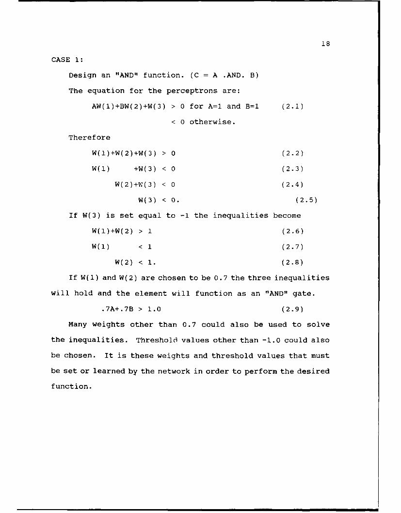
CASE 1:

Design an "AND" function. (C = A .AND. B)

The equation for the perceptrons are:

AW(1)+BW(2)+W(3) > 0 for A=1 and B=1 (2.1)

< 0 otherwise.

Therefore

W(1)+W(2)+W(3) > 0 (2.2)

W(1) +W(3) < 0 (2.3)

W(2)+-W(3) < 0 (2.4)

W(3) < 0. (2.5)

If W(3) is set equal to -1 the inequalities become

W(1)+W(2) > 1 (2.6)

W(1) < 1 (2.7)

W(2) < 1. (2.8)

If W(1) and W(2) are chosen to be 0.7 the three inequalities

will hold and the element will function as an "AND" gate.

.7A+.7B > 1.0 (2.9)

Many weights other than 0.7 could also be used to solve

the inequalities. Threshold values other than -1.0 could also

be chosen. It is these weights and threshold values that must

be set or learned by the network in order to perform the desired

function.

19

CASE 2:

Design an "OR" function. (C = A .OR. B)

The equation for the Perceptrons are:

AW(1)+BW(2)+W(3) > 0 (2.10)

AW(1) +W(3) > 0 (2.11)

BW(2)+W(3) > 0 (2.12)

W(3) < 0. (2.13)

If W(3) is set equal to -1 the inequalities becomes

W(1)+W(2) > 1 (2.14)

W(1) > 1 (2.15)

W(2) > 1. (2.16)

If W(1) and W(2) are chosen to be 1.5 the three inequalities

will hold and the element will function as an "OR" gate.

1.5A + 1.5B > ! (2.17)

If negative weights are allowed an inverter can be

implemented with a single weight equal to -1. Since the

functions AND, OR, and INVERT can be implemented with

perceptrons any logical function can be implemented with them.

It is very important to note that even though all logical

functions can be implemented with perceptrons they cannot all

be implemented in one level. It was demonstrated by Minsky

and Papert [1] in their book "Perceptrons" that the EXCLUSIVE-OR

function can only be implemented with two or more levels of

perceptrons. Consider the following problem.

20

CASE 3

Design an "EXCLUSIVE-OR" function (C=A .XOR. B)

The equations for the perceptron are:

AW(1) + BW(2) + W(3) < 0 (2.16)

AW(l) + W(3) > 0 (2.19)

BW(2) + W(3) > 0 (2.20)

W(3) < 0. (2.21)

Combining (2.19) & (2.20) yields

AW(1) + BW(2) > -2W(3). (2.22)

Combining (2.22) & (2.18) yields

AW(1) + BW(2) > -W(3) + AW(1) + BW(2) (2.23)

0 > -W(3) OR W(3) > 0. (2.24)

Since it is known from Equation (2.21) that W(3) < 0, the

problem will not have a solution with one perceptron.

The property of perceptrons not inability to perform the

EXCLUSIVE-OR function in one level is of much importance

historically and practically. This function is required in

many problems. If the problems are complex it will be desirable

to train the network rather than design it mathematically.

Until recently it has been extremely difficult to train these

multilevel networks. New advances in training using

backpropagation have greatly enhanced the ability to train

multilevel ANNs.

21

2.2 Types of Artificial Neural Networks

When studying the biological neural networks that comprise

the cerebral cortex, it is found to be able to perform many

functions. Among their basic functions are pattern recognition,

sound recognition, speech comprehension, logic, associative

memory, generalization, and interpretation of sensory input.

[17] Different neuron models and different network

configurations have been proposed to provide the best emulation

of different neural functions.

Some of the most common network configurations are:

Feedforward Networks, Hopfield Nets, Bidirectional Associative

Memory, Adaptive Resonance Theory, and Counter Propagation.

Some of these configurations require special training

procedures or special neuron models. The weights in these

networks are adjusted in one of two major ways:

(1) by calculation or

(2) by training.

Training is also divided into two main categories:

(1) supervised training and

(2) non-supervised training.

In supervised training known inputs are applied to the network

and the outputs are observed. Adjustments are then made to

the weights in order to change the prevailing outputs into the

desired outputs. After many training sets have been applied

and weights have been adjusted, the network will respond in

22

the desired manner. In non-supervised learning various training

sets are applied to the input of the network. As different

features are recognized by the network it will adjust its

weights so different input patterns can be categorized. When

new input patterns are applied the nearest category to the

input will be indicated by the output.

There is some concern among researchers as to whether

certain network configurations or learning paradigms should

be used based on how realistically they actually model

biological neural networks. Some researchers believe that

when designing a machine that emulates human brain functions,

it is best to remain as close as possible to an accurate

biological neural network. Others contend that as many

liberties as are required should be taken in order to best

solve the problem being studied. The latter philosophy will

be used in the dissertation.

2.2.1 Feedforward Networks

Feedforward networks or nonrecurrent networks are one of

the most common neural networks used today. A feedforward

network consist of one or more rows of artificial neurons.

The inputs to the first layer come from the sensory outputs.

If more than one level is incorporated in the network design

the outputs from each element of a previous level are fed

forward into the inputs of each element of the next level.

23

The connections can be fully connected or sparsely connected.

With fully connected networks each neuron takes its inputs

from every neuron or sensor in the preceding level. In a

feedforward network no neuron is allowed to feedback to a prior

level. An example of a fully connected feedforward network

is shown is Figure 7.

INPUTS OUTPUTS

SENSORS LEVEL i LEVEL 2

HIDDEN UNITS

Figure 7

Fully Connected Neural Network

The neurons in the network that precede the output level

are referred to as "hidden units". These hidden units can

pose difficulties in training since their outputs cannot be

measured directly. Feedforward networks have some important

attributes. One of these attributes is their ability to be

unconditionally stable. There is no feedback in the network.

An input vector will simply propagate through the network and

24

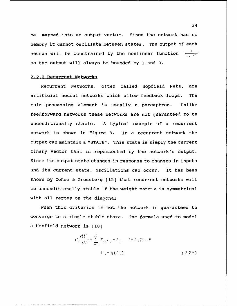
be mapped into an output vector. Since the network has no

memory it cannot oscillate between states. The output of each

neuron will be constrained by the nonlinear function -

so the output will always be bounded by 1 and 0.

2.2.2 Recurrent Networks

Recurrent Networks, often called Hopfield Nets, are

artificial neural networks which allow feedback loops. The

main processing element is usually a perceptron. Unlike

feedforward networks these networks are not guaranteed to be

unconditionally stable. A typical example of a recurrent

network is shown in Figure 8. In a recurrent network the

output can maintain a "STATE". This state is simply the current

binary vector that is represented by the network's output.

Since its output state changes in response to changes in inputs

and its current state, oscillations can occur. It has been

shown by Cohen & Grossberg [15] that recurrent networks will

be unconditionally stable if the weight matrix is symmetrical

with all zeroes on the diagonal.

When this criterion is met the network is guaranteed to

converge to a single stable state. The formula used to model

a Hopfield network is [18]

-- I l~ + i= 1 .2...I'd, I I

V (1(L 1).(2 .25)

25

Where C is the input electrical Capacitance of the

operational amplifier used to model the

artificial neuron.

V, is the neuron output.

Ui= the neuron input.

Tij are the weights (synapse strength).

(For the network to be guaranteed stable

T:i=O and Tij=Tj,).

g is a nonlinear function.

The energy of the network that converges to a minimum value

is given by the Liapunov function [18]

FEEDBACK LOOPS

OUTPUTSINPUTS

SENSORS

Figure 8

Recurrent Network

26

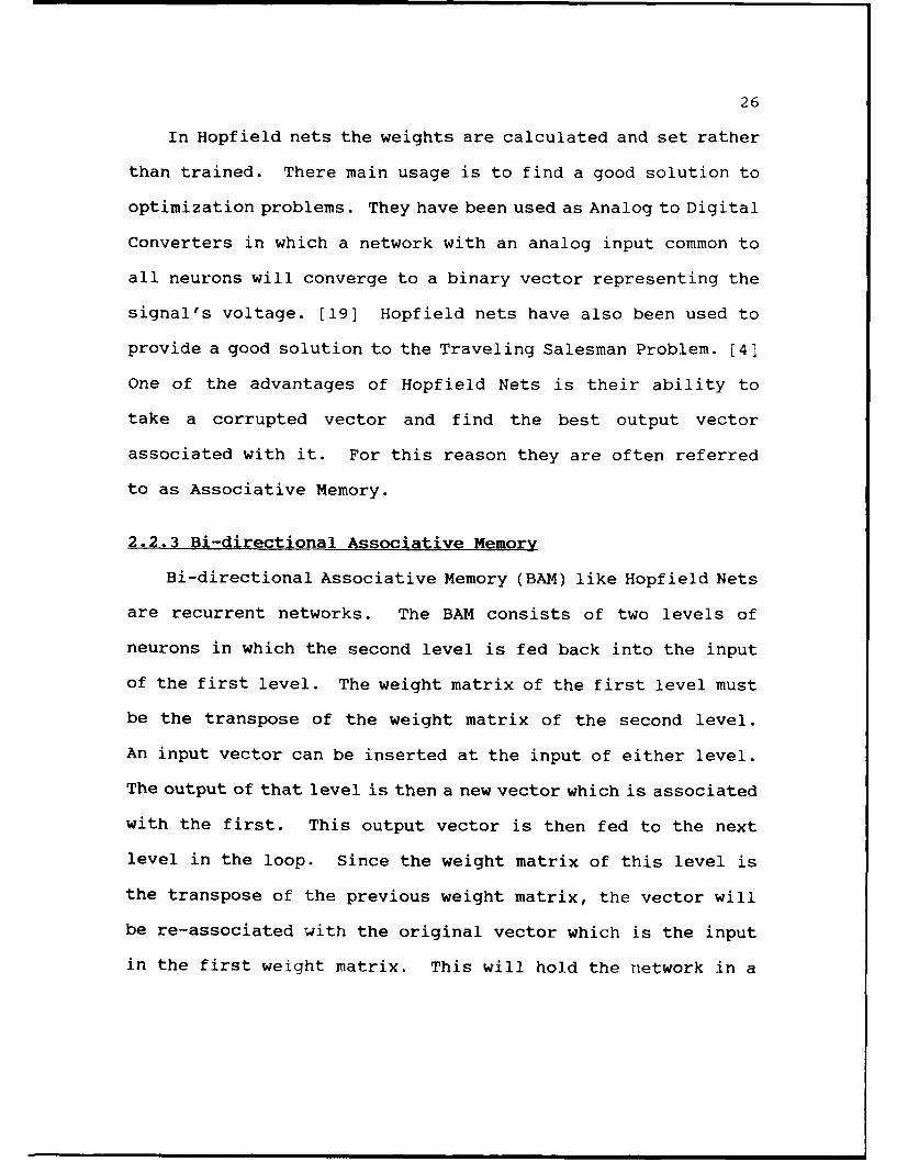
In Hopfield nets the weights are calculated and set rather

than trained. There main usage is to find a good solution to

optimization problems. They have been used as Analog to Digital

Converters in which a network with an analog input common to

all neurons will converge to a binary vector representing the

signal's voltage. [19] Hopfield nets have also been used to

provide a good solution to the Traveling Salesman Problem. [4]

One of the advantages of Hopfield Nets is their ability to

take a corrupted vector and find the best output vector

associated with it. For this reason they are often referred

to as Associative Memory.

2.2.3 Bi-directional Associative Memory

Bi-directional Associative Memory (BAM) like Hopfield Nets

are recurrent networks. The BAM consists of two levels of

neurons in which the second level is fed back into the input

of the first level. The weight matrix of the first level must

be the transpose of the weight matrix of the second level.

An input vector can be inserted at the input of either level.

The output of that level is then a new vector which is associated

with the first. This output vector is then fed to the next

level in the loop. Since the weight matrix of this level is

the transpose of the previous weight matrix, the vector will

be re-associated with the original vector which is the input

in the first weight matrix. This will hold the network in a

27

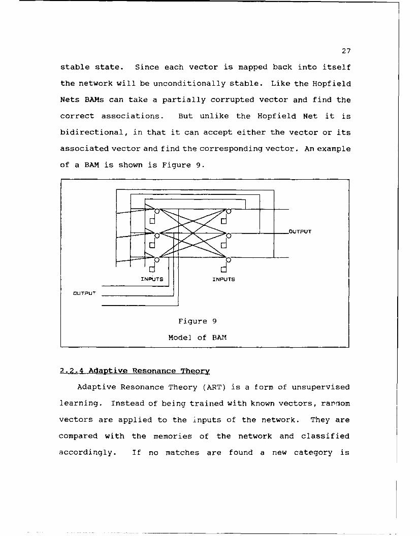
stable state. Since each vector is mapped back into itself

the network will be unconditionally stable. Like the Hopfield

Nets BAMs can take a partially corrupted vector and find the

correct associations. But unlike the Hopfield Net it is

bidirectional, in that it can accept either the vector or its

associated vector and find the corresponding vector. An example

of a BAM is shown is Figure 9.

H 0 0 OUTPUT

INP6TS INPUTS

OLJTPUT

Figure 9

Model of BA14

2.2.4 Adaptive Resonance Theory

Adaptive Resonance Theory (ART) is a form of unsupervised

learning. Instead of being trained with known vectors, rar'om

vectors are applied to the inputs of the network. They are

compared with the memories of the network and classified

accordingly. If no matches are found a new category is

28

generated. This network model has the advantage of not requiring

that an associated output vector be known for each input vector.

It learns to classify vectors based on similarities recognized

in the training set. This model is similar to biological

neurons, in that it does not require a supervisor in order to

learn. This ability to learn without supervision can be

disadvantageous. In many cases the features being extracted

from the input vector may not be the most obvious. In these

cases supervised learning could provide a solution while ART

would fail.

2.3 Training

Training is the method by which the weights of a neuron

are modified in order to learn the correct network response.

There are two major ways of training networks; statistical and

deterministic. Deterministic training has evolved from the

Delta Rule to more useful me~-hods such as Backpropagation.

In order to train a neural network using supervised

training, a set of known vectors must be input into the network

and the outputs must be compared with the known results. Based

on the correctness or error in the result the weights of the

network are adjusted. Training can be a very time consuming

process. One problem, that is common to both biological and

artificial neural networks, is their tendency to forget. When

a set of patterns are presented to a network and weights are

29

adjusted to provide correct results, it is found that the first

patterns will usually be forgotten by the time the later

patterns are presented. This problem can be partially solved

by repeatedly presenting all the patterns many times.

2.3.1 The Delta Rule

One of the most important training methods is the Delta Rule.

With the Delta Rule the weights of each neuron are adjusted

by using the following algorithm:

( I I') h +(n)+K ,\ INPUT (2.27)

A.7 AkCF7 - , 1. (2.28)

where W(n+l) is the new adjusted weight.

W(n) is the old weight.

K is the training rate.

(usually between 0.1 and 1.0)

X ARET is the known result that corresponds to the input.

Xxwxu1 is the input to the neuron.

Xou1 is the output response to input XxmvuT with

weights W(n).

It can be noted from the above formula that when the error

term (XRG - Xou-r) is zero, no weight modification will

occur. When this term is not zero, training will occur in the

direction and strength that is proportional to it. It should

also be noted that when no input from Xxtu- excites the neuron

30

no modifications are made to the weight associated with this

input. This means that if this input did not contribute to

the error, its weight should not be modified. This algorithm

can be used to train perceptrons in single level networks or

multilevel networks in which desired outputs for each level

are known. However, multilevel networks in which the outputs

for the hidden units are not known present serious problems.

In 1969 Minsky & Papert proved in their book "Perceptrons" [1]

that many important functions such as EXCLUSIVE-OR or Parity

could not be solved in a single level of perceptrons. This

combined with the difficulties encountered in training

multilevel networks did much to deter research on neural

networks during the 1970's. However in 1986 several

researchers, Rumelhart, Hinton, and Williams developed a

training method for training multilevel networks known as

backpropagation or the Generalized Delta Rule. Backpropagation

was also discovered by Werbos in 1974, and Parker in 1982, but

a book by Rumelhart and McClelland [3] gave a particularly

detailed explanation of these training rules. This discovery

has done much to rekindle interest in neural networks in the

1980's.

2.3.2 Backropagat on

Backpropagation or the Generalized Delta Rule provides a

method of training all of the weights in a multilevel feedforward

31

neural network. The method of training the weights is a

gradient descent method. The change in th- error of the network

is calculated with respect to each weight. This value is the

slope of an error curve like the example shown in Figure 10.

F 1

Global Minmum4k i

is

N

7E T (2.29)

F, = (-T - Or) (2.30)

where Erork is the total error from the N patterns,

32

Er- is the error from pattern P,

T is the target output value,

0 is the output value.

It should be noted that when only one pattern is presented

the total error will equal (T-0)', which will form a parabolic

curve similar to the example in Figure 10. This parabola has

a minimum value known as the "global minimum".

The equations modeling neuron (j) are

Q -,f \ 1+1,) (221

~ = \~ h ,,_ (2.32)0I1

where wij is the weight connecting the output of

neuron (i) to neuron (j).

NET is the internal summation of the weighted inputs

to neuron (j).

and f is the nonlinear function

For the output level of the network the error slope can

be calculated as follows.

aF~ ~ F Fp P___ - ___ = \_ p (2.33)

ah, alli ,al

By using the chain rule the derivative of the error due to one

pattern with respect to any weight can be expressed as:

33

a a 1J, ao0 ahN

I)1 d ) dA - ) 3 1"

Carrying out these differentiations will yield:

S =- 2(1-- 0) /(.ET). . (2.3)

al '

The derivative of the nonlinear function f(.-)= is.(2.36)

So the formula for adjusting the weights is

=--2.( -(T 0,).(f(0 , FT)).(I-/f(.A FT)) .0,. (2.37 )af 11

Since the correction to weight Wij is proportional to the

negative derivative of the error, the correction formula will

be

A , ,, l ( :-o,) f[( \FT)(i-/( \ FT)).O0. (2.3B)

Where K is the learning rate.

The real power of backpropagation is its ability to train

the hidden units of the network. The training equation must

be modified since the target values, Ti, are not known fora F

hidden units. First b is defined as ". In terms of the

output units it can be expressed as

bf,, = - 2" (I -0)/( \ "( .T). (2.39)

The training formula is \h =k.bO,. From the chain rule the

definition of 6p, can be modified to be

34

dEFpdP, = Opl . '(NETP,). (2.40)

By using the chain rule again, E can be rewritten in terms

of the previous level's NETs

b) 1 7 Ep dNETPk. f'(NETPJ) (2.41)

= aNETpk bOp,

OR

bP = 3E ."hkI" f'(. ET P ) " (2.42)

K aNETpk

From the definition of 6 for an arbitrary level the formula

can be rewritten as

k

6 / 6 ,pk hkJ f(%'ET P) (2.13)

OR

k

bpj= f'(NETP,) I6,k " ',I (2.44)

The training formula for hidden units is then

AIV,J= K '60 ,= K 'O ," f'(NETp,) E bpk'h 'kI. (2.45)K

The weights are adjusted by adding the correction to the current

weight values.

4/,,(n + I )W= i,(n)+ Avi, (2.46)

The weight changes are often modified by adding a momentum

term. The momentum term acts as a low pass filter to limit

35

oscillations in the training session. It is applied to the

equation as follows.

A[",,= K'6"O+ "Ah' "'M (2.47)

Where M is the momentum term.

The choice of a momentum term, M, and a learning rate term,

K, is very important when training a network. If K is too

small the training can take a tremendous amount of time to

converge. If K is too large oscillations can occur and prevent

conversion. Extreme values of M can also affect the time of

convergence. Good values for these constants are usually 0.1

to 1.0. The best values to which the weights should be

initialized are small random values. Care should be taken to

ensure that all weights are not set to the same value. If

they are set to the same value and a fully connected network

is used, all weight change calculations will yield the same

value and all weights will remain equal to one another throughout

the training session. During a training session the weights

could possibly fall into a state with all equal wieghts, but

this would be extremely rare. Adding extremely small amounts

of noise to the weights after each training iteration can

prevent this state from developing.

There is a very important problem that often counteracts

the improvements gained by using backpropagation. This problem

is the ability to fall into a "local minimum". These "local

36

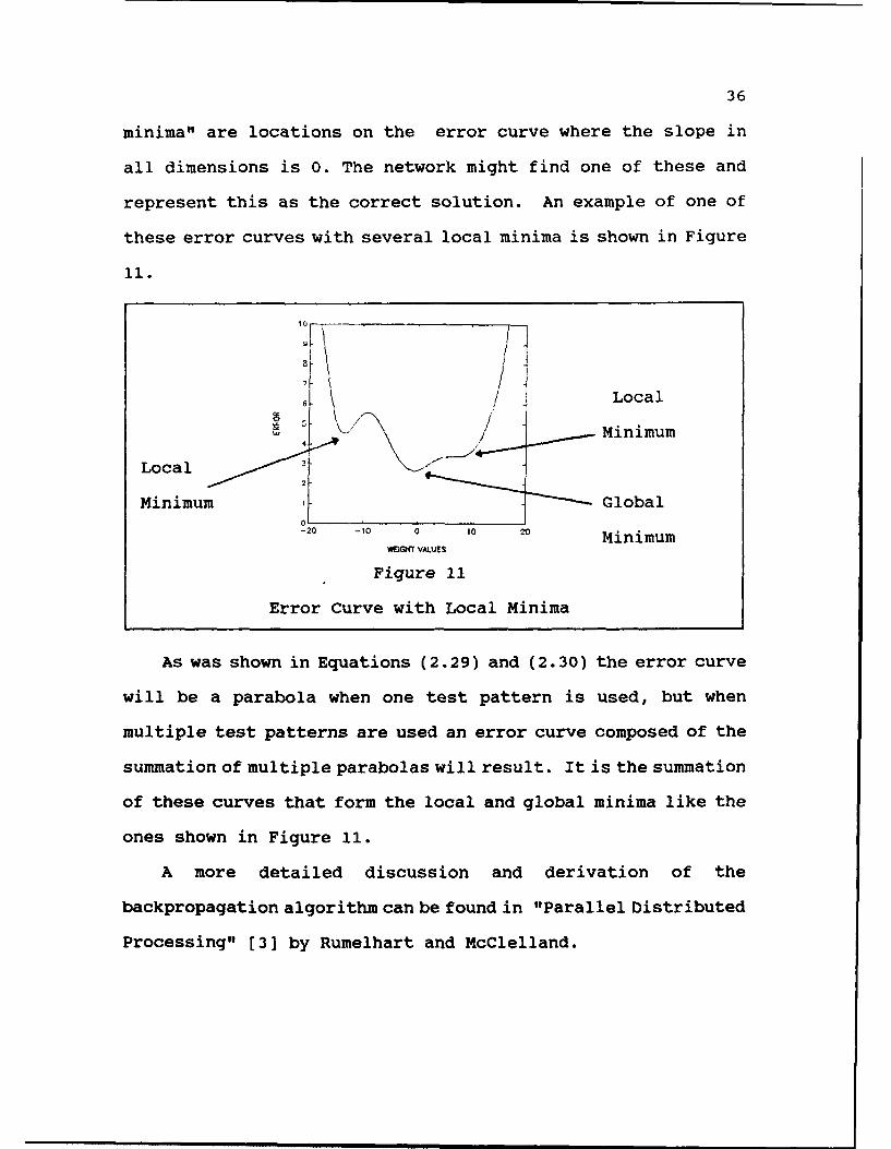
minima" are locations on the error curve where the slope in

all dimensions is 0. The network might find one of these and

represent this as the correct solution. An example of one of

these error curves with several local minima is shown in Figure

11..

6 1 ILocal

/ minimum

Local

Minimum Global

-20 -10 0 ,0 2 Minimum

Figure 11

Error Curve with Local Minima

As was shown in Equations (2.29) and (2.30) the error curve

will be a parabola when one test pattern is used, but when

multiple test patterns are used an error curve composed of the

summation of multiple parabolas will result. It is the summation

of these curves that form the local and global minima like the

ones shown in Figure 11.

A more detailed discussion and derivation of the

backpropagation algorithm can be found in "Parallel Distributed

Processing" [3] by Rumelhart and McClelland.

37

2.3.3 Statistical Training

Statistical training is a method of randomly adjusting

weights that eliminates many of the local minima. The basic

procedure is: [4]

(1) Place a vector on the input of the network.

(2) Measure the total error in the output.

(3) Select a weight at random.

Change its value a small random amount.

(4) Re-measure the error.

(5) If the error is decreased keep the change.

Otherwise retain the original weight.

(6) Repeat the procedure until a suitable solution is

reached.

This procedure is analogous to the annealing of metals in

the way it moves from a high energy state to a minimum energy

state. Therefore it is often referred to as "simulated

annealing". Another form of statistical learning is known as

Boltzmann's Training. In this form the changes, C, are

determined by the formula

/AI (2.48)

where K is the Boltzmann constant.

T is an artificial temperature determined by

1(I) = 0 /Ioql(I +1). (2.49)

To is the initial temperature,

38

and t is time.

2.4 Linearly Separable Regions

It has been demonstrated in an earlier section how the

perceptron can be used to perform simple logic by using one

level of perceptrons. These perceptron equations with variables

A and B take the form:

WxA + W2B + W3 > 0 or (2.50)

WxA + W2B + W3 < 0. (2.51)

The equation WxA + W2B + W3 = 0 describes a straight line.

The perceptron therefore can be used to separate points above

the line from those below it. If three inputs are used in the

perceptron this line will become a plane in three dimensional

space. If N inputs are used it will be expanded into N

dimensions and define an N-i dimensional hyperplane that divides

an N dimensional hypervolume. When additional levels of

perceptrons are used the complexity of the pattern being

distinguished can be increased. A two-level network for

example can be used to separate any convex region from its

background. Three levels of neurons can be used to separate

any regions regardless of their geometry. Consider the

following example shown in Figure 12.

39

C

NPUT2

E \D

INPUT I

Figure 12

Example of Linearly Separable Region

One perceptron could be used to separate points above line

AB, another to separate points to the left of line CD and

another to separate points below EF. If a second level of

perceptrons is used to "AND" the outputs of the first three

perceptrons, the convex region can be separated from all other

points. An example of a convex region is shown in the shaded

area of Figure 12. Any region or set of regions can be divided

into a set of convex regions. A third level of perceptrons

can then be used to "OR" together the convex regions and thus

separate any regions from all other points.

This provides a very powerful tool for use in pattern

recognition problems. With this ability a network can be

designed and trained to separate any pattern from its background

40

or another pattern. The network will be unconditionally stable

and its output will be bounded by 1 and 0. It can be implemented

in only three levels of perceptrons and will operate in realtime

with a propagation delay of only three delay units. Where a

delay unit is the propagation delay per level of perceptrons.

There are however several major problems with this form

of network:

(1) Training times can be extremely long when backpropagation

is used.

(2) The number of hidden units required to work difficult

geometries can be very high.

(3) The training solution can fall into a "local minimum".

Chapter 3

Beamformer Fundamentals

3.1 Basic Types of Beamformers

Beamformer arrays are used in a variety of different

applications. The array can be of any size, but the basic

operation is usually one of two functions. Either the

information received by the array is processed in order to

indicate the direction from which a wave is approaching or if

the direction is already known, the information is processed

by steering the beamformer in the direction oi the wave. If

the wave is steered toward the source of the signal, noise

from other sources will partially cancel and an improved signal

to noise ratio of the signal of interest will be realized.

3.2 Narrowband Beamformer

When a wavefront approaches an array of sensors like the

one shown in Figure 13, the array will sample the wave in space

as well as in time. If instantaneous measurements are recorded

on all N sensors, and if the wave is a single frequency sinusoid

41

42

the resulting vector can be represented by the following

equation

I, =SIN(wt + i). (3.1)

2r. -I SIN(0)where a =

and 21i is the wvav'e number.

cu is the waves f requency.

d is the distance between sensors.

X is the wavelength.

0 is the arrival angle

and t is time.

WAVE

W% .A. \

'S ' 'S% S .V , "

ISENSORStf

Figure 13

Beamformer Array

Therefore at any instantaneous point is time with the

signal frequency held constant, the output, Vi, viewed over

space will be a sinusoid whose phase is determined by the

43

arrival angle, 0, 'he distance between sensors, d, and the

wavelength, A.

The angle of approach, 0, can be determined by analyzing

the space sampled information. The output of this analysis

will be a function of both the angle of approach, the frequency

of the wave being studied, and the propagation speed of the

media through which the wave is traveling. If the propagation

speed and the wave frequency are known, the angle of approach

can be determined from the space sampled data.

One implementation often used to process the output of a

beamformer array consist of an operational amplifier used to

sum the output. If N sensors are summed the resulting output

will be:

0! fF1 T= ,= \(ct ± ) (3.2)

0! /f [ I COS ( (A\-1) 1') fo oI\ 7a ,

01 /!I I \ 'SI\(cl) for c=0. (3.3)

The amplitude of this output is the term

I t= \ 10 (=0 (3.4)

This output will be a maximum when a =0 (when the wave is

parallel to the line of sensors and perpendicular to the

44

boresight). This is known as the steered direction. Depending

on the number of sensors, N, the output may have several

sidelobes which can allow noise from directions other than 0

degrees to interfere with the received signal.

If it is desired to know the direction from which a signal

propagates, multiple beamformer arrays could be used. These

arrays could each be aligned in the direction perpendicular

to the direction it was designed to observe. The array with

the highest output would indicate the direction from which the

wave was approaching. A more practical method would be to

process the information from the same array through multiple

operational amplifiers each of which is designed to respond

to a different angle of arrival. This steering can be

accomplished by placing an appropriate time delay at each input

to the operational amplifier so the summation equation will

be

N-iY= S IN (w(t-,A,) + a ). (3.5)1.0

Where A, is the time delay.

If w, is equal to ai the beamformer will be steered toward

angle 0. Since a= the delay should therefore be set

for

45

2nidSIN(O) (3.6)(A

dSIN(0)

PROPAGATION VELOCIY (3)

Another way of accomplishing beamformer steering is by

multiplying the signal by P-1" in order to shift it by the

appropriate phase. (i is the sensor index and j is \<-).

1'-0I = [sl\((t+a)]K- ' ° ' (3.8)

N'- I -j

= 2- [SIX(w t)+jCOS(wt)] (3.9)

The phase of the sine wave will no longer be a function of the

wavenumber, <Y. Therefore the steering can be accomplished by

multiplying the sensor's output by the weight h ,=o - a'. This

phase adjustment seems to be the simpler of the two methods

but the weight's value will be a function of (). This will

not present a problem if (k) is a constant, but if (A) varies

and covers a large bandwidth additional processing will be

required.

3.3 Wideband Beamformers

When the operation of a beamformer over a large bandwidth

is desired, changes to the beamformer processing must be made.

Since the frequency of the wave is not constant the resulting

sensor output will be a function of CAk as well as 0.

46

', = SN(g(w,1)+ f(O.i)) (3.10)

From equation 3.1

Implementation of wideband beamformers is sometimes

accomplished by bandpass filtering the output of each sensor

into narrow bands and then processing each band through a

narrowband beamformer. An example is shown in Figure 14.

INPUTSSENSORS

BANOPASSFILTERS

NARROW-BANDBEAMFORMERS

OUTPUTS DIRECT ON I DIRECT ON 2 DIRECTION 3 DIRECTION 4

Figure 14

Wideband Beamformer

When the direction of a wavefront is known and it is desired

to focus on the signal source, steering can be accomplished

by placing time delays in the lines. This can be performed

just as was done with narrowband beamformers. However, a phase

delay cannot be used to shift the phase since the phase is a

function of frequency and the frequency is not constant. In

47

order to process these wideband signals they must be filtered

into narrow bands and processed separately. One novel method

of implementing this filtering and subsequent phase shifting

has been reported by Follett [5]. This method incorporates

the use of Discrete Fourier Transforms or Fast Fourier

Transforms to process the digitized sensor outputs.

3.4 Previous Work

An extensive amount of literature has been published over

the past two decades on beamformer arrays. Specialized systems

for seismic, sonar, radar, and radio telescope arrays have

been reported and analyzed. [16] Three of these systems which

represent the progress in beamformer arrays and Neural Networks

are described below. First one system using an FFT beamformer

is described. Another form of these beamformers which uses

the earliest form of artificial neuron, the ADALINE, is also

discussed. Lastly some more recent research combining both

beamformers and Hopfield Networks is presented.

3.4.1 Fast Fourier Transform Wideband Beamformer

One method f processing wideband beamformer arrays is

with a Fast Fourier Transform (FFT) Beamformer. [5] With such

a system an FFT or Discrete Fourier Transform (DFT) is performed

on the output of the sensor data. This first DFT filters the

data into narrowbands. The output of each frequency band is

then routed to another Fourier Transform where the space sampled

48

data is transformed into a domain which represent the wave

number of the space sampled signal. It should be noted that

the equation used to add the phase delay to the sensor outputs

is

V -

V = N\ - . (3.1!1)

t-I

This equation is mathematically equivalent to the Discrete

Fourier Transform which is

V-I

Fk = VfIIek (3.12)1-0

If the number of time samples and the number of sensors are

a power of two an FFT can be used to calculate these shifts.

The data can then be re-routed to an Inverse Fourier Transform

where it can be transformed back into the time domain.

To demonstrate the use of Fourier Transforms in processing

beamformer arrays, the angle response of a narrow band signal

was plotted for 9 bands. The DFT was evaluated at equal phase

increments which translated into arrival angles of 0.0, 7.18,

14.48, 22.02, 30.00, 38.68, 48.59, 61.04, and 90.00 degrees.

These values were calculated from Equation (3.1).

2ndSIN(O) (3.13)

or

o=SI( i d(3.14)

011,

49

If the sensor distance, d, is set equal one half the

wavelength, I>, the formula reduces to 0 = SIX'N . As the phase

varies from 0 to if the arrival angle, 0, will vary from 0 to

90 degrees.

The bandwidth can be determined by the following formula

taken from Follet [5].

B -~ .886y-s ( ). .i [V /Iijli (3.15)

01"

1\\ =2 .8 (> n(ar endkir 8j (3.1 Y)

A table that shows the relationship between phases arrival

angles and bandwidth is shown is Table 1.

Phase Arrival Angle BandwidthDegrees Degrees Degrees

0 0.00 5.0820 6.38 5.1140 12.84 5.2160 19.47 5.3880 26.39 5.67

100 33.75 6.11120 41.81 6.81140 51.06 8.08160 62.73 11.08180 90.00 34.00

Table 1

Bandwidth of Arrival Angles

It should be noted that the spacing of d was set equal to

one half the wavelength of the wave. This wavelength is a

50

function of the frequency of the wave and the velocity at which

it travels. This selection of sensor spacing, d, tunes the

array to work at a specific frequency. If wideband signals

are to be detected, modifications to the system must be made.

One solution to this problem can be achieved by using multiple

arrays of sensors known as sub-arrays. The output of each

sensor in each array is converted into the frequency domain

with a DFT or FFT. When the data is routed to the next level

of the FFT beamformer only the frequencies corresponding to

the sub-array's tuned frequency will be included in the routing.

There are several problems that should be noted with the

DFT method of processing. First there are sidebands that

could be mistaken for the main signal. Secondly, when equal

phase increments are used, (which is a requirement for FFTs)

the resulting arrival angles will be defined sharply for lower

angles and very coursely for higher angles. When the wave

direction is not known it will be more useful to have equal

arrival angle detection. An FFT narrowband beamformer example

is shown in Figure 15. The angle response of a wideband

beamformer is shown in Figure 16. In this example 20 sub-arrays

were used to analyze data with a bandwidth of 30 to 300 Hz.

This wideband example is clearly inferior to the narrowband

example. FFT beamformers have several important advantages.

They have the capability of detecting signals from different

51

SARRIVAL ANGLES 67.6 - 90.0

C-2

3, o a- s . do. io. do. doT. 100'@.w. 1. ~0 do. ANGLE - EGREES

SARRIVAL ANGLES 54~.5 67.6

A .NGLE -D EGREES5 0 o o ,0

' ARRIVAL ANGLES 43.8 - 53.4

0 C9 .1,20.4. do o ~ d. do .

ANGLE - DEGREES

_ARRIVAL ANGLES 34.6 -42.7

10. o. 30. 40. 0.4 0. 0o. 0 . 10

RRRP4ALGL ANGES .6. - 5.

~ RBRIVAL ANGL ES 11.2 - 25.4

do. 40. do. do.~o. do. do. 100.ANGLE- ERES

-ARVLANGLES 41.0 17.8

Jo o. Jo. 40. o o. voo. --- o. 1 aoANGLE - DEGREEL

ARR~IVAL ANGLES 4.0 103.2

- 3 N

Jo 0 . 40 0. )w . do. 0o. 100.

Figure 15

DFT Narrowband Beamformer Resporse

52

SARRIVAL ANGLES 67.6 - 90.0

QOJ. 10 o2. 30. ,40. ).m. . T. . 100.ANGLE -DEGREES

~ARRIVAL ANGLES t4.5675.6

ANGLE - EGREES

~ARRIVAL ANGLES 34.6 42.7

4. 10. do. .4o. d. 0.ANGLE DEGREES

MAIVAL ANGLES 26.3 -33.7

ARRIVAL ANGLES 18.6 -25.4

~J 1.1.@. 40. qO. do. To.do . 100.ANGLE DEGREES

ARRIVAL ANGLES 4.0 10.4

1 10@. TO 00.. i laANGLE -DEGREES

ARRIVAL ANGLES .0 - 3.2

Figure 16

DFT Wideband Beamformer Response

53

directions concurrently. They also can provide a time history

output. This can be of great importance in determining not

only the direction of the signal but its signature as well.

The FFT beamformer plots are presented with the appropriate

3 db passband superimposed on each plot. The 3 db passband

is the band between the half power points. These half power

points are the locations where the signal is attenuated by a

factor of 0.707.

3.4.2 Adaptive Beamformers with ADALINES

Artificial Neural Networks have been used in the form of

ADALINES in numerous applications. Many of these have been

reported by Widrow, the inventor of the ADALINE, and Stearns.

[7] The ADALINE is primarily an adaptive filter. In beamformer

arrays they can be used to adapt for noise cancelation or array

steering. In many of these applications the least-mean-square

(LMS) algorithm is used. This is the algorithm on which the

Delta Rule was based. In this algorithm the square of the

error is minimized by adjusting weights on the ADALINE until

an optimum filter has been adapted. A pilot signal is often

used to provide a source with which to train the network.

These networks provide an analog output just as the FFT

beamformer method does. When a pilot signal is used to train

the network, it will allow the network to adapt to interference

or noise signals that can be unique to a particular environment.

54

3.4.3 Beamforming with Hopfield Networks

Methods of using Hopfield Networks to determine the angle

of arrival have been reported by Park [20], Rastogi, et al

[21], and Goryn and Kaveh [28]. A summary taken from their

work follows. In these efforts the wave number of a narrowband

signal or the frequency of a time sampled signal can be

determined. Multiple frequencies can be determined with the

network shown in Figure 17.

INPUT (I)___________________________JWEIGHTS7 7 DETWEEN

I OUTPUT & INPUTS

RESIS-0P PESI TOP PES TOP

CAPACITOR CAPACITOR JAPACITOR

OUTPUT (V)

HOPFIELO AND TANK NEURAL NETWORK MODEL

(FROM GORYN & KAVEH 12B]

Figure 17

Hopfield Network for Beamforming

In this network the input is a function of frequency,

phase, and amplitude. The output is a 1 or a 0, which corresponds

to the presence or absence of a signal in the form: ( taken

from Rastogi's derivation [21])

55

jO /0 w 12w ;.V w

S = [0,1 ...... P e o ] for frequency detection (3.17)

or

12- I( )f I(l-1) SIN(n)flSi , .'n-SR ),s (3.18)..... i ............. V

for ri l an le detection.

The error to be minimized in the network is

: = Y -I , S ..... 3 19

Where y is the analog input

Si is the signal vector described above.

V is the binary output vector.

Manipulation of this formula can be shown to yield

F ='y+l I' SI-yS -1 -S . (3.20)

Since Equation (3.20) is being minimized with respect to V,

terms without V can be removed.

/-,-=I 'SIS[-2 . (y'Sl ) (3.21)

Since Tii=0 for stability the term must be subtracted

This equation can be further manipulated to become

. s2(< ,)I. I , - (2 '.,+Ss,) I . (3.2;3)F<>1

56

(t is the transpose conjugate & T is the transpose)

Comparison of this formula with the energy function for the

Hopfie'd Net,

F I /,I I)

shows that the feedback weights, T, should be equal to

/, = -2 l , i (3.2u5)

and the input weight should be

I I .1 1J .16i, =X S - " } 11'2s

The weights for the feedback can be calculated from the known

values of Si. However the weights for the inputs must be

calculated from the input vector and the Si vector. When the

network converges, each output neuron will take on an output

value of 1 or 0 indicating the presence or absence of a wave

of the corresponding amplitude, phase, and frequency.

Simulations made by Rastini, et a] [21] were very successful

in detecting the input's frequency spectrum when the SNR was

5 db.

This network has a very important advantage when used to

detect angles of arrival, in that it can detect multiple arrival

angles. The network can also provide very fine accuracy in

the angle being resolved. There are however several important

disadvantages. One is the problem of setting the weights for

57

the network. The inputs weights are a function of the input,

yL. This means that the vector multiplication between y and

S must be performed for each input set. The network also

requires a large quantity of neurons. One for each combination

of angle, phase, and amplitude to be detected. Park and Rastogi

have both reported ways of reducing this number of neurons,

but considerable preprocessing is still required. Goryn and

Kaveh have extended the procedure to include wideband signals,

but preprocessing is still required including a DFT on the

input data. An example of the angle response of a narrowband

beamformer designed with an Hopfield net is shown in Figure

18. This network was designed using 50 gages and 90 neurons

for 90 evenly spaced arrival angles. The network was tested

by generating a signal of each angle and processing it through

the network with 12 iterations of the following formula.

S/ ( )' [ (f)10 '; Ic() ll oll l lll l i (1 1 ) I.

This formula is a discrete version of Equation (2.25) which

models the Hopfield network.

In Figure 19 an example is shown in which three different

arrival ngles are presented to the network. These angles

were 10, 50, and 62 degrees. After 6 iterations all three

angles were correctly identified.

58

When training examples can be submitted to a network in

order to teach it the proper response, an important improvement

can be realized. All of the beamformer algorithms presented

so far consider a situation in which the propagation speed is

constant and the wave is approaching from one direction. This

may be accurate for some applications but for many others the

propagation speed will vary if the media through which it

travels is not homogeneous. Reflections and echos are of a

considerable consequence in both seismic and sonar

applications. To address these problems more thoroughly

feedforward networks can be trained with known signals to

provide beamformers which adapt to the environmental

characteristics and provide a more accurate response.

59

ARRIVAL ANGLES 80.0 - 90.w

A. RI .A. . .70. o. 6o. AG. E. DGE.ANGLE DEGREES

ARRIVAL ANGLES 760.0 - 70.0

w..10. 40, d.. . 10.ANGLE DEGREES

SARRIVAL NGLE5 0.0 - 70.0

tiAVR NGE 5 .1- 6 .

-4I

. 20. o. 4 . . .. .

ANGLE DEGREES

ARRIVAL ANGLES 0.0 0.0.4

6!

~~. 10. 0. do3. 4 0. 0 0. 7. d. d. i

ANGLE OE(tREES

ARRIVAL ANGLES 20.0 - 30.0

0. 40. . --0 . S . . so. do. ,00.

ANGLE - EGREES

ARRIVAL ANGLES 10.0 20.0

0 1. l. - 30. 40. 50. 0.-- .

100.

ANGLE DEGREES

. ARRIVAL ANGLES 2 ,0 - 0.0

40.. to. W do . - - . 0. ... . 20.

ANGLE GEGREES

Figure 18

Angle Response of Hopfield

Net ANN

60

ITERATION 9

(L'

J. , . . . A. do. )o. do. do. io.ANGLE - DEGREES

5!-ITERATION a

Q. . . Jo. . q. do. o. do. 0. wo0.ANGLE - DEGREES

ITERATION 7

Jo. 40. do. )W. do. do. too.ANGLE "DEGREES

-ITERATION 6

iTR. IO 1'0 dO.ERS o 9. do. do. ?00.ANGLE -wDEGREEo

ITERATION 5

.-1

1.it. oo. 09. do. do. 'lea.

ANGLE " DEGREES

ITERATION 3

I. do. do. aO.GL d.. DEGESo" 90. do. do. i'0.

ANGLE .DEGREES".

ITERATION 2

ANGLE ObErAEH )0'

ITERATION I

ANGLE - DEGREES

Figure 19

Hopfield Network Detection of 3 Angles

Chapter 4

Model of Narrowband Beamformer

4.1 Beamformer Array Processing with ANNs

Artificial Neural Networks provide an interesting way of

processing the information received from beamformer arrays.

When the desired application is one of determining the direction

of the received signal, ANNs offer several advantages over

digital signal processing networks. Rather than requiring

special processing modules such as analog to digital converters

or special digital signal processing circuits the ANN provides

a system which will accept the sensor's analog output and

produce a digital output that represents the presence or absence

of a wave received from a designated direction. ANNs operate

in realtime with very small propagation delays. However, ANNs

lack the precision and qualitative results that can be provided

with conventional methods of signal processing. As will be

demonstrated, ANNs offer good performance in the presence of

both random and correlated noise. They also offer good immunity

to variations in amplitude.

61

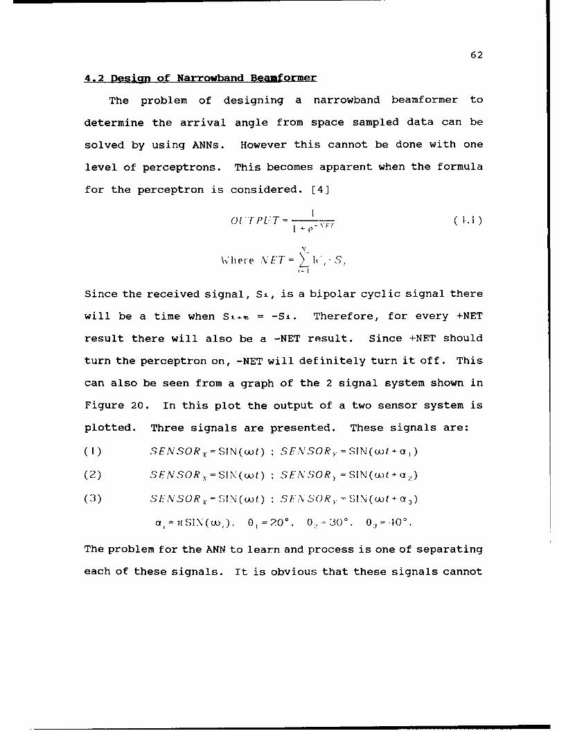
62

4.2 Design of Narrowband Beamformer

The problem of designing a narrowband beamformer to

determine the arrival angle from space sampled data can be

solved by using ANNs. However this cannot be done with one

level of perceptrons. This becomes apparent when the formula

for the perceptron is considered. [4]

OUTPUT -= I V T ( .1)

N

_

\khere \.' T= Ih ,. S,

Since the received signal, S±, is a bipolar cyclic signal there

will be a time when S±t-o- = -Si. Therefore, for every +NET

result there will also be a -NET result. Since +NET should

turn the perceptron on, -NET will definitely turn it off. This

can also be seen from a graph of the 2 signal system shown in

Figure 20. In this plot the output of a two sensor system is

plotted. Three signals are presented. These signals are:

(1) SENSORx=SIN(wt) : SENSORY SIN(ut+a 1 )

(2) SFNSOR,=SIN(t) , SENSOR,.=SIN(ckt+ 2)

(3) SENSORx=SI\N(cwt) SE ,NSOR = SIN(ooit+cf

a , = TiS IN ( u,), 0 , =2 0 °0, 0 ;?= '30 0. 03 = 40 .

The problem for the ANN to learn and process is one of separating

each of these signals. It is obvious that these signals cannot

63

be linearly separated. There is no way one straight line can

be drawn separating any of the curves into two linearly separable

regions.

ARRIVAL ANGELS

40 DEGREES

30 DEGREES

20 DEGREES

Figure 20

Graph of 2 Signal System

In order to design a narrowband beamformer multiple

perceptrons will be required. It is suggested that this can

be done by dividing the waveform to be analyzed into segments

and then designing each perceptron in the first level of the

network to key on one and only one segment of the waveform.

The segments which make up the desired response are then OR'ed

together with a final perceptron. An example of such a network

is shown is Figure 21.

64

4 SEGMENToDEN UNITS

INPUT I3NPUTa [ OUTPUT I

INPUT 2

INPUT 3

OUTPUT 2INPUT 4

INPUT M OUTPUT N

Figure 21

Segmented Network

In this chapter four methods are used to demonstrate how

the weights for the network can be found. These methods are:

(1) By Mathematical Analysis.

(2) By training each level of the network separately with the

Delta Rule and knowledge of what the output of each level

should be.

(3) By Backpropagation training.

(4) By using preprocessing of the sensor inputs and

Backpropagation.

4.3 Mathematical Analysis of Beamformer

When the approximate formula of the input signal is known,

a mathematical analysis can be performed and values for the

weights can be calculated. The basic conditions to be sqtisfied

65

for each of the arrival angle bands, 0, and time segment, t,

are:

(1) OiTPLT = f(NET)= I for 02>0>01 ald 11 >1>t2

(2) OUTPUT = f(NET) = 0 for 02<0 and for all t

(3) OUTPUT f(\FET) - 0 for 0 >0 and for all t

(4) OUTPUT = (N ET) - Don t Care OtherwNise.

Since the sigmoid function, /(AFT)=I , is monotonically

increasing and bounded by 0 and 1, it will approach 1 as NET

becomes very large and 0 as NET becomes very small.

Therefore for f(NET) to equal 1 the following inequality

must be satisfied.

\/:l>*>0: \I'T=>h,,S-TI tlOID" S =.SI\(ut+ia,)

01"

\ 1 B./ K.';Il\Qut+ ici) >> IttI~hSIIOI.D (-t.2)

For f(NET) to equal 0, the opposite of the above inequality

must be solved.

VI, B • CI\( t + IcR) <lfllIfOI. (1.3)

2ii d S I \ (0)Q' =

A

Where 0 is the arrival angle,

N is the wave length.

B is the amplitude of the waveform.

d is the distance between sensors.

66

To minimize the error, the formula

' 0+i2ndSIN(O) >> THRES H I D (, 4.1)

should be maximized for 0 1<0<02, and the formula

SV B SI\(I + 21(dSIN(O)}<<THRESIHIOD I.)

should be minimized for 02<0<900 and 0OO<O, for all t.

The expected values of these formulas are found to be

0 2 t 2

E 1 - J 1(0) /(t) V,. B SIN(ut+ia)dtd0 (1.6)'Il

(2n ci)a = SIN(O).X

where f(o) and (t) are probability density I u nctions.

The probability of any arrival angle, 0, or time segment, t,

of the sine wave is usually a uniform distribution. The result

of the integration yields

(4.7)

011 1 ' ' f!:'I,]=o~2_ )02-01 1". WI B(COS('t 2 +ic*)-COS(u't +ia))dO"

This formula can be solved by composite numerical integration.

The maximum values for the function OUTPUT VLIsC,f(i) should

occur when they are fully correlated with f(i)=Wi. Therefore

the weights are calculated to be equal to the above formula.

67

To demonstrate the effect of these weights the equation

can be tested with the known signal, -.I S1\(it+at). The output

of the neuron can be expressed as

O1 T-P1 T1 (\ / .( .8)

uhoro \l=l> X..i.Si\(uIt-ai).h,.

Substituting the calculated values for W, into this formula

and writing tx and t2 in terms of the width of the time segment

and the center of the time segment yields:

2iu/

Ot-TPtT- -: (1.9)

I +B

0 - . 0 .9 5 l \ ( t ,) . l ~ / t ) I / + 1 ) O ( .10 )

\ /"1! O,-()))b

1

Qt It (). t,

It can be noted that this formula will provide high values

proportional to A, and ' \((u!,). Therefore the more hidden

neurons that are used to subdivide the waveform into small

time segments, ti, the higher the neuron's NET output will be.

A plot of this formula's response is shown in Figure 22.

In this example the formula is evaluated with 0 aii 0 equal

to 20 and 30 degrees respectively. The time segment was

centered at zero, (t-=0). The phase can be calculated from

68

the arrival angle by the formula This plot of the

perceptron's output as a function of time and arrival angle

demonstrates that the neuron fires when the signal is in both

the correct angle bin and time segment bin. The plot also

demonstrates that when the signal is outside the correct angle

bin the result will be zero.

'/ -. ' Z.. -- • -' - -".\ --------.- ------ -- --

.-

Figure 22

Mathematically Designed Response

One problem should be noted. No matter what angle is being

applied to the perceptron, there can be times when the amplitude,

A, can be high enough to cause the neuron to excite.

After the outputs of each segment are calculated, they are

OR'ed together using one perceptron to provide the desired

output. The plot in Figure 22 does not necessarily represent

69

the optimum solution to the problem. It represents only one

of many possible solutions and could be one of the local minima

into which a backpropagation routine can fall.

4.4 Results of Mathematically Designed Beamformer

Several simulations were made using the weights derived

with Equation (4.7). Each simulation set consist of 9

simulations for 9 different arrival angles. These arrival

angles were 0-10, 10-20, 20-30, ... 80-90 degrees. The

simulations were made using 10 sensor inputs and 2, 3, and 20

hidden units. Plots of these simulations are shown in Figures

23, 24, and 25. Simulations were also run for networks with

4,5 and 10 hidden units. These networks showed very little

difference to the ones with 3 and 20 hidden units.

These plots demonstrate that when the number of hidden

units is incieased to around 4 the network's ability to determine

the correct direction is greatly improved. The plots also

demonstrate that the lower arrival angles can be identified

more accurately than higher arrival angles. A comparison was

made between the FFT narrowband beamformer shown is Figure 15

and the mathematically designed beamformer in Figure 25. The

percent of correct responses for the FFT beamformer was 97%

while the mathematically designed beamformer was only 76%.

This was primarily due to the mathematically designed

beamformers poor performance for high arrival angles. A

70

comparison itemized by arrival angle is shown in Table 2. It

should be noted that the mathematically designed beamformer

is designed to detect equal arrival angles but the DFT beamtormer

detects equal phases.

Arrival % Correct, % Correct,Angle DFT Math

Beamformer Beamformer(20 Hidden Units)

0 to 10 92.750.0 to 3.17 98.33

10 to 20 86.813.98 to 10.38 96.67

20 to 30 87.3611.2 to 17.75 97.22

30 to 40 84.6318.6 to 25.45 97.22

40 to 50 71.6926.3 to 33.66 97.22

50 to 60 68.4234.6 to 42.75 96.66

60 to 70 61.5843.7 to 53.38 96.11

70 to 80 63.9254.4 to 67.59 96.67

80 to 9O 66.8367.6 to 90. 99.44

Table 2

Comparison between Beamformers

71

2 RRRIVAL ANGLE5 80.0 - 90.0

10. 20. 30. ,0. : . d0. 0. Bo. ..ANGLE DEGREES

I V9, HN6LE5 70.0 - 60,0

-- I101 i' . 2,0. 30. , _. 0 Q) . ' .

ANGLE DEGREF5

-.PRR!VRL FIGS E. 70.0

ANGLE - DEGREES

.RR 2VA0 NGLE5 t .0 F0 ..

L.0. ." ,,. d,,

II

50. 60. . -E 5E

• / /

.. - ~~~~. , . , : :

. . . ' . ,, ' 2. ',. - . '77VN - " ,F 1 '

Figure 23

Mathematically Designed ANN Using 2 Hidden Units

72

SARRIVAL ANGLES 0. 90.

CLAAViLAGE 7iz

ANGLE DEGREES~ ARMIVAL ANGLES 7zi.z 60.0

o7 ~. 0. q. doi. To dzi .zANGLE - DEGAEES

SAAAIVAL ANGLES z0.0z 70.

ANGLE -DEGREES

~ARRIVAL ANGLES 50i.0 60.0~z

ANGLE b EGAEESSAAAIVAL ANGLES MO 50.0

ARIA ANLS 300 4.

ANGLE -DEGREES

~AAAIVAL ANGLES 20i.2 30i.0

CA-I

ANGLE - DEGREES2 RAIVRL ANGLES 10i.0 20.

2*4 'k__. __.

ANGLE -DEGREES

SfIAR I VAL ANGLES .0 10.0~z

IT0. o. 0. A NGLE D EGAFFS 0 o10

Figure 24

Mathematically Designed ANN Using 3 Hidden Units

73

. ARRIVAL ANGLES 80.0 - 90.0

ANGLE DEGREES

ARRIVAL ANGLES 70.0 - 0.0

ANGLE - DEGREES.ARRIVHL ANGLE5 60.0 - 70.0

1. 'o. Jo J . .. 0. d.o 1,00.62 RRIVA.L ANGLES 50.0 -6.0

ANGLE - DEGREESARRIVAL ANGLES 40.0 - 50.0

0. 10. 20. 30. 40. 5. 5. 7. 6. 2. 10

ANGLE DEGREESARAIVAL ANGLE5 30.0 - t0.0

0. 1. 20. 30. 40. to.S 0. 70. 60. 9. 10

aNGLE CEGREESARRIVAL ANGLES 20.0 - 30.0

*= _. _._ _ --,... .0. a. 30. 40 . S . - . 0. 2. 7oz.

ANGuS - 2.A3EE.

NGL5 10.0 20.0

o -:z. 0. ,.so. 70. ?2. 2. 100.HNG.E DEREES

" i~ P %.CS .a ;.

40. . 0. 0. 0. .0. J 9. 00.PN;i DEGREES

Figure 25

Mathematically Designed ANN Using 20 Hidden Units

4.5 Delta Rule Training of Narrowband Beamformer

74

The first training method that will be used to train the

narrowband beamformer is the Delta Rule. When using the Delta

Rule each level is trained independently based on knowledge

of what that level's output should be. The network shown in

Figure 26 is used.

INPUT I 4 SEGMENT HIDDEN

UNITS

INPUT 2 FIRST LEVEL

SECOND LEVEL

INPUT 3

INPUT 4OUTPUT 2

INPUT M

Figure 26

Narrowband Beamformer for One Arrival Angle

Many neural network models are divided into two main

sections. The first section performs "feature extraction" to

separate the data's important characteristics needed by the

second level. The second level is the network that learns to

process these features and learns the correct response to

different stimuli. The networks in Figure 26 can be considered

to be such a system. The first level extracts the features

which are the different time segments of the angle to be

75

detected and the second level is trained to give the proper

response.

To implement this model each arrival angle band is trained

separately. Every input sensor is connected to every hidden

level neuron. Each hidden level neuron is designed to respond

to the presence of one segment of one arrival angle band. The

outputs of the hidden units within a segment are then combined

in the second level to provide an output that represents the

presence of a signal within the arrival band at any time. The

following procedure is used to train each of the networks.

(1) Equation (4.7) is used to calculate the weights for

each secment of the first level.

(2) The last level is trained using the Delta Rule to

provide an optimum set of weights for the final level.

This method is a very practical method of training the

network. When the output of the hidden units can be determined

by training or analysis, the Delta Rule will provide a fast

method of calculating optimum weights for the final level.

4.6 Results of Training with the Delta Rule.

The network designed in the previous section was used to

simulate the same three configurations presented in the previous

section. The first level was trained using Equation (4.7).

Tie network was implemented using 2, 3, and 20 hidden units.

Simulations using 5 and 10 hidden units were also implemented,

76

but they were almost identical to the simulations conducted

with 3 and 20 hidden units. The final level was trained with

the Delta Rule. A learning rate between .1 and .3 and a

momentum term of .9 were used in the learning algorithm. These

values were chosen by trying various sets and noticing which

ones caused the network to converge faster. The rate of

convergence and the minima, local or global, to which the

network converges is a function of the input patterns used to

train the network and the random values to which the weights

are initially set. Since the values are not deterministic,

they must be approximated from experimental results.

Adjustments to the weights were made after every pattern was

presented to the network.

The results of these three simulations are shown in Figures

27 through 29. These plots indicate that when the final

perceptrons are trained to find optimum weights for this last

level the results will be improved. These plots are still far

from ideal. The highest angles are still very erroneous and

the transition bands are not sharp. When the weights for the

first level of perceptrons were calculated, it was assumed

that each element should represent an equal time segment. This

was not a good assumption. It would be desirable to allow the

first level of perceptrons to train also so they could find

values that were more near the optimum level. A comparison

between the mathematically designed beamformer and the Delta

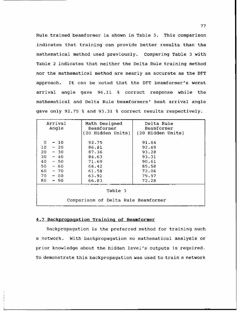
77

Rule trained beamformer is shown in Table 3. This comparison

indicates that training can provide better results than the

mathematical method used previously. Comparing Table 3 with

Table 2 indicates that neither the Delta Rule training method

nor the mathematical method are nearly as accurate as the DFT

approach. It can be noted that the DFT beamformer's worst

arrival angle gave 96.11 % correct response while the

mathematical and Delta Rule beamformers' best arrival angle

gave only 92.75 % and 93.31 % correct results respectively.

Arrival Math Designed Delta RuleAngle Beamformer Beamformer

(20 Hidden Units) (20 Hidden Units)

0 - 10 92.75 91.6410 - 20 86.81 92.6920 - 30 87.36 93.2830 - 40 84.63 93.3140 - 50 71.69 90.6150 - 60 68.42 85.5860 - 70 61.58 72.0670 - 80 63.92 79.9780 - 90 66.83 72.28

Table 3

Comparison of Delta Rule Beamformer

4.7 Backpropagation Training of Beamformer

Backpropagation is the preferred method for training such

a network. With backpropagation no mathematical analysis or

prior knowledge about the hidden level's outputs is required.

To demonstrate this backpropagation was used to train a network

78

ARRIVAL ANGLES 80.0 90.0

O k ~ 0.r 4 10 .. Q ~

ANGLE - DEGREES-"ARRIVAL ANGLES 60.0 - 0.0

6000

'R RRIVAL ANGLES 5I0.@ 7 0.0

1. 7 . TO 4.0. 0. 0. 1060.

ARRIVAL ANGLES 5W0.0 - 60.0 NL ERE

ANGLE -DEGREES

SARRIVAL ANGLES 40.0 5 '0.0

Q. 0.ANGLE bFDGREES~ARRIVAL ANGLES 30.0 - 0.0

* 7 7~i~ .(a.~ Ia. lot.ANGLE D)EGREES

~ARRIVAL ANGLES 20.0 30.0

ANGLE bDCEF5E

'2ARRIVAL ANGLES .0 10.0

ANGIE SER-

Figure 27

Delta Rule Trained ANN with 2 Hidden Units

79

SARRIVAL ANGLES 80.0 - 90.0

0. 1. 20. o. 40. )0 0.~ . do. do. 0.oANGLE -DEGREES

~ARRIVAL ANGLES 70.0 -601.0

loI. do. 4o. '0o . din. )0. do. 40. 1 01D.ANGLE -DEGREES

89 RRIVAL ANGLES 60.0 70.10

i'O. do. Jo. 40. qO. d. 0- -7 o. -do. do. 100.ANGLE -DEGREES

SARRIVAL ANGLES 40.0 - 6OJ.0

10O. 20 0. 40. do. 6 )2o. . do. 1,o0.ANGLE -DEGREES

_HARHIVAL ANGLES 40.0 - 4.0

0. 1. 20. 0. 40. SO. doo0. 6. do. 100.ANGLE DEGREES

HRRIVAL ANGLES 20.0 - 3.0

0. 10. 20. 30j o. do0~ . do. do. 100.ANGLE DEGREES

~ IRVtANGLES 10.0 - 30.0

ANGLE DOEGREEs* RHIVA. FNGLE 1.0 2 0.0

0. 10. Q. Io . q0. do. dz. do. '100.ANGLE DEGREES

Figure 28

Delta Rule Trained ANN with 3 Hidden Units

80

SARRIVAL ANGLES 80.0 -90.@

3.0J. 40qo o. d. ioAINGLE DEgREAS

M RRIVAL ANGLES 70.0 8 0.10

=I

~ d. d. 'o. s. o. o. do. do. 7210.ANGLE O EGREES

~ARRIVAL ANLEIC 60.0 70.0

-- ----------- T-- ------- r- -- - -T-- ______o. 1 . 0 . 4. . 0. . 7 io. ioz.ANGLE DEGREES

SARRIVAL ANGLES 50.0 -60.0

ANGLE -DEGREES

'!ARRIVAL ANGLES 40.0 -50.0

ANGLE - DGRE L

SARRIVAL ANGLES 30.0 -40.2

:0.T -o o o d. d. 9. Yo-- . ,30.ANGLE DEGREES

~ARRIVAL ANGLES 20.0 -30.0

ANGLE - DEGRE 5

~ARRIVAL ANGLES !0.0 .20.0

1. 1. 0o. Jo. a0 di 0.~ . do . do. :MoANGLE bEGREH

SARRIVAL ANGLES .0 10.0

ANGLE bEGREE

Figure 29

Delta Rule Trained ANN with 20 Hidden Units

81

comparable to Figure 26. In this network two levels of neurons

were used as shown in the network of Figure 30.

4 SEGMENT HIDDEN UNITS

INPUT I M INPUT UNITS

INPUT 2PUT UNIT

INPUT 2

OUT PUTINPUT 4 L

INPUT M

Figure 30

Narrowband Beamformer

Two levels were used since it is known that any convex

pattern can be separated from its background in two levels.

Backpropagation can be especially important for several

reasons. The input signal is not always one for which a simple

algebraic formula is known. There can also be nonlinearities

in the media through which the data propagates. Mechanical

or electrical noise can also add complexity to the problem.

Problems emanating from sensor coupling, calibration,

linearity, or placement can also complicate a formal analysis

of the problem. When the problem is very difficult, the use

of a mathematical analysis for determining weights is arduous.

82

However when data from known sources are used to train the

network, it will learn the effect of the nonlinearities and

adjust the weights accordingly.

4.8 Results of Training with Backpropagation

Backpropagation was used to train the same network used

in the Delta Rule Training section and the Mathematical

Simulation Section. Again 2, 3, and 20 hidden units were used.

In these simulations the average value of the network output

is plotted. This average is taken over an entire cycle. This

is accomplished by evaluating the network output at 20 random

times and computing the average. These results also demonstrate

that performance is improved when more hidden units are used.

They also indicate aqgin that the response at higher arrival

angles is poor. Since the phase is related to the arrival

angle by the formula - the phase difference will be

much smaller for higher angles bands that lower ones. This

would require a much sharper separation for the higher angles.

The results of these simulations are shown in Figure 31 through

33. Since the highest two arrival angles are the most difficult

to train, an inaccurate response was learned in the 70 to 80

degree angle bin. The results of these simulations are shown

in Figure 31 through 33.

A comparison of the backpropagation trained network, the

Delta Rule trained network, and the mathematically trained

83

network is shown in Table 4. This comparison shows that the

backpropagation method and the DFT method are very similar

when used as a narrowband beamformer. The DFT beamformer

outperformed the backpropagation beamformer is 3 of the 9

arrival angle bins. It shoud be noted that the DFT beamformer's

arrival angle bins were approximately 5 degrees wide compared

to 10 degrees for the backpropagation beamformer.

Arrival Math Delta Backpro- DFTAngle System Rule pagation System

System System

0 - 10 92.75 91.64 99.22 98.33 beam 110 - 20 86.81 92.69 98.33 96.67 beam 220 - 30 87.36 93.28 98.39 97.22 beam 330 - 40 84.63 93.31 98.25 97.22 beam 440 - 50 71.69 90.61 97.69 97.22 beam 550 - 60 68.42 85.58 97.00 96.66 beam 660 - 70 61.58 72.06 94.44 96.11 beam 770 - 80 63.92 79.97 90.42 96.67 beam 880 - 90 66.83 72.28 97.11 99.22 beam 9

Table 4

Comparison with Backpropagation Beamformer

Simulations were also made in which wider ranges of amplitudes

were used. In these simulations backpropagation was used to

train the same three networks used in the previous simulations.

Amplitude ranges of .5 to 2.0 were used to test the network

more stringently. The plots of these simulations are shown

84

~ARRIVAL ANGLES 80.0 -90.0

sJ 10. 0.. 0.100. !.

0.. i. 0.. 100.ANGLE -DEGREES

ARIVAL ANGLES 70.0 8 0.0

10.Y~ 20. 0. 40. qo. do. o o ~~10ANGLE -DEGREES

'2 ARI1V1L ANGLES 50.0 76.

AR IA0AG E . ( 6 ..

Jo10. !O. d . )@ o o 100.ANGLE - DEGREES

SARRIVAL ANGLES 40.0 !j

4,.d . o o . 2

ANGLE DEGREES

ARRIVAL ANGLES 30.0 -40.0

9. 0'. 0. lo. 40. . do. )@. do. do. ' 100.ANGLE DEGREES

'!-ARRIVAL ANGLES 20.0 - 30.0

~~ ~ANGLE lobFGRE o. o'--~. 10

-ARRIVAL ANGLES 10.0 - 20.0

Q. .0 . o 40. d. do. 0. 0. .ANGLE DEGREES

~ARRIVAL ANGLES .0 10.0

ANGLE -DEGAFES

Figure 31

Average Output of Backpropaqation ANN with 2 Hidden Unitsi

85

~ARRIVAL ANGLES 80.0 -90.0

0. 1. 20. 30. 40. )0 o. 9. do. do. 100.ANGLE -DEGREES

SARRIVAL ANGLES 70.0 - 0.0

0. lo o. Jo. do. )0ERES 9. do. do. 10

SARRIVAL ANGLES 60.0 -70.0

J0 o. do. qo. do. . 9o d.ANGLE -DEGAEES

SARAIVAL ANGLES 50.0 - 60.0

10o. )0 o o d. d. 9. do. d. £oANGLE - DGREES5

'. ARRIVAL ANGLES 4l0.0 t0.0

i'o. Jo. 10. 40. E. o. 9o. do: (D. Oo.ANGLE - EGREES

do. 4'0. d. d. o do. 1100.ANGLE -DEGREES

6 ARRIVAL ANGLES 20.0 - 30.0

0. o. 20. Jo. 0. qo. do 9. do o. I'MoANGLE - DEGREES

2 ARRIVAL ANGLES 10.0- 20.0

t'o. )o. do. '0 . d. ~ . 9. d. ~ . 1ANGLE -DEGREkt

H9ARIVAL ANGLES .0 10.0

0. 10. 0. 0. '0. .. 0. d0. 0. 0.

Figure 32

Average Output of Backpropagation ANN with 3 Hidden Units

86

ARRIVAL ANGLES 80.0 9.

4. ~ ~ ~ ~ 10 0.0 0 0

ARRIVAL ANGLES 70.0 -IGE bGE

-IL

aa-

ANGLE -DEGREES' 0 0ARRIVAL ANGLES 50. 7@@ ANL

ANGLE DEGREESARRIVAL ANGLES 50g.0 0.

RRItVAL ANGLES 40.@ 5@Q-NL ERE

IU. ~ 0. ~ g. NGLE 'a bEGREE'S' ~

ijRRIVAL ANGLES WZ~ - .Z

ARRIVAL ANGLES 2 .e 2 30.2 ANGLE T E A~ g g

a.. ae. 'b EG

A4WNGLE -EGRE ES '

Figure 33

Average output of Backpropagation ANN with 20 Hidden Units

87

in Figure 34 through 36. These plots indicate that a network

will perform better, if an automatic gain control is used to

restrict its amplitude to a narrow range.

The network was also tested for its sensitivity to noise.

The peak to peak noise level was set for .2, .4, and .8 on the

simulations shown in Figure 37 through 39. These networks

used 5 hidden units and an amplitude range of .5 to 1.0. This

amplitude choice was taken from a uniform distribution. The

uncorrelated noise level was also taken from a uniform2

distribution. By using the formula S\R= 10 .0O0 .' these

noise levels will correspond to a SNR of 19.42 db, 13.34 db,

and 7.38 db respectively. These three simulations provided

results that were 93.46%, 91.03%, and 81.52% correct. These

results show a very serious degradation in response as the

signal to noise is decreased from 13.34 db to 7.38 db.

DFT beamformers also degrade as the SNR is decreased. Since

the DFT beamformer is an analog system, its performance can

be measured by comparing the input SNR to the output SNR. Both

the DFT beamformer and conventional beamformers have an array

gain improvement on the order of 10log(N), where N is the

number of sensors. [5]

88

SARRIVAL ANGLES 80.0 - 90.0

ANGLE - DEGREE .~ARRIVAL ANGLES 7C.10 - 0.0

,*0.ANGLE O EGREVS

~ARRIVAL ANGLES 60.0 -70.0

110. 0 0. 40. do d '. do. do. ilia.

~ARRIVAL ANGLES 50.0 -60.0

~~~~.NL AMUVL NGES 400 35.

ARRIVAL ANGLES 40.0 5 '0.0

im0.~ . Ia. 40. To. do. )@. do. do. 100.ANGLE - EGRE ES

'! ARRIVAL ANGLES 20.0 - 3.0

~~~-C ARIVA ANLE 10.,300.

4~bERE 10)0 o o. d. d. 9. do. do. fe0.ANGLE - EREt

SARRIVAL ANGLES 1.0 2 0.0

do ). do. do. 'iw

Figure 34

ANN with 2 Hidden Units and Amplitude Range of .5-2.

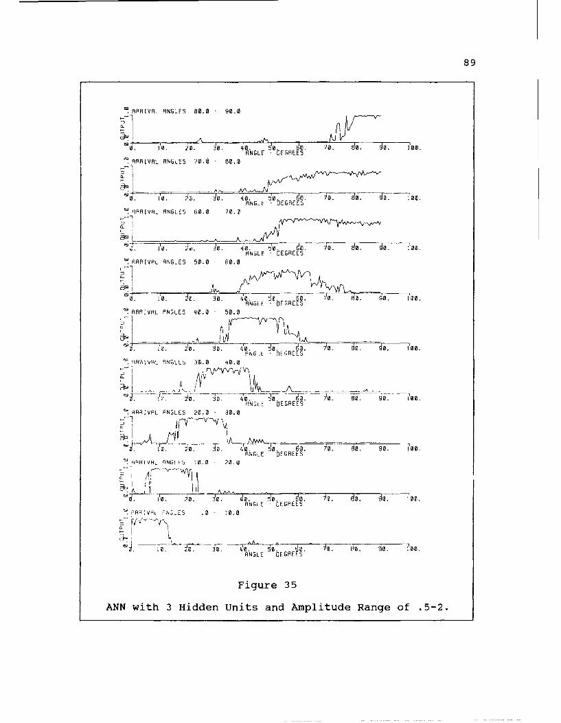
89

ARRIVAL ANGLES 80.0 90.0

S . .- .NGLE . DEGREES 90 . .

do.10. )0. .. do. 100.ANGLE - DEGREES

ARRIVAL ANGLES 60.0 70.0

. j. do. 40. . do. )o. do. do. 1o.

ANGLE DEGREES

ARRIVAL ANGLES 50.0 70.0

.. ['0. 0. 0,. 4. ?0. 0. 0. 80. 0. 100.ANGLE -DEGREESAR IVAL ANLE 0. 00.

ANGLE rGREES'

ARRIVAL ANGLES 40.0 50.0

I ____ _______

0. 10. 0 . do. )o. do. do. 'o.ANGLE DEGREES

. RR! L SLE U.2 4z@

PNGLE - DEGREESARRIVAL ANGLES 20.0 - 30.0

ANGLE DEGREES! ARRIVAL ANGLES 10.0 - 20.0

0. 0 qo d. )o. do. do. 00o.

RNGLE DEGREESSARHIVRL ANGLES ,. - 10.0

(00.

ANGLE DEGREES

Figure 35

ANN with 3 Hidden Units and Amplitude Range of .5-2.

90

'ARRIVAL ANGLES 80.0 -90.0

~ 1. 10 0. )W.'1. do. do 0 . too.ANGLE - EGRE S

HHAHIVML riNGLE3 70.0 69.0

ANGLE -DEGREES*. ARRIVAL ANGLES 60.0 70.0

Al

0. M. 10 . 4 40. do. )M. do. do . o00.ANGLE -DEGREES

RRIVAL ANGLES 50.0 -60.0

d '. 10. 0. ;0. d10 0. D. 02. do. do. 'o.

~ RRIVAL ANGLES 4T0.0 -50.0

a. .t o o.'. d oo. Todo do. ?00o.ANGLE -DEGREES

ARRIVAL ANGLES 30.0 4 '0.0

~o o 4. d. do. )2. do. do. 100.ANGLE -DEGREES

ARRIVAL ANGLES 20.0 -30.0

iw.~o d. to. do d. o. do. -do. 'loc.ANGLE - DEGREKE

ARRIVAL ANGLES 10.0 20.0

ANGLE - EGREfES'ARRIVAL ANGLES .0 -10.0

0Jo

HNGLE DoEGREES- @ o e

Figure 36

ANN with 20 Hidden Units and Amplitude Range of .5-2.

91

ARRIVAL ANGLES 80.0 90.0

0. 10. 0. ~ ANGLE DEGREES d

AAIVAL ANGLES 70.0 60.0

. 21. 10 4Q. ,. do. (10.

ANGLE DEGRELS

ARRIVAL ANGLES 60.2 70.0

Q 'o. . 4. o. do. 9o. d . 'o. 10'.ANGLE - DEGREES

ARRIVAL ANGLES 50.0 60.0

4o. 0~. d. Mo od. do. 1,20.ARRIVAL ANGLES 40.0 50.0

I.O 20." . 40. 5o. d 0. do. do. 100.ANGLE DEGREES

ARRIVAL ANGLES 30.0 40.0

'O. )0 10 4--- 40. o. do. do. do. '100.ANGLE DEGREES

AR' IVAL ANGLES 20.0 30.0

- I

to. j. 4 .H d. )o. do. do. 1oo.ANGLE DEGREES

HRRIVRL HNGLES I.0 - 20.0

S -. o. 3 . o. do. . do. ,. 1'00.ANGLE -DEGREES

"HHVRL AV 6 LE5 .0 10.0

J. Y. do. do. -0. d,. do. -o. do.- do. to.ANGLE DEGREES

Figure 37

ANN with 2 Hidden Units and Noise of .2

92

ARVLANGLES 80.0 - 90.WqW

1W 2. W. ANGLE - EGREk go' aW. loo'. W

~ARRIVAL ANGLES 70.0 - O.0

ep RVLANLS E. -7

ANGLE - EGREESHHRRIVRL ANGLES 60. - 70.0 . W . 0. . 0. L.

10. ~ W. ~ W. 40. 2. do. )3. ~ . ~ . IANGLE -DEGREES

~ARRIVAL AN'GLES 50.0 6 0.o

ANGLE -DEGREESdo

HHRHRVAlL ANGLES 40.0 5 0.0

~W. ~ W 40 di ~ W. ~ . dO. do. LWANGLE -DEGRE S

SARRIVAL ANGLES 20.0 40.0

1Wlo W W ~ W o W . d~o. l~~~~.IL ARRIVA ANLS 1.5-2.

~.ARRIVAL ANGLES 2.0 3 0.8

0-

1W. )a. Ia. ri. m0~. do. 9. I'm.

FiGuE 38GAANVA NGE with 3 HidnUnt0ndNie f.

93

SARRIVAL ANGLES 80.0 - 90.0

0. 10.REE 20)0 O. U .~ . do. do. 1,20.

SARRIVAL ANGLES 70.0 - 0.0ANL DERE

1,20

ANGLE DEGREESR RRIVAL ANGLES 60.0- 70.0

10 o 0.~ . d. )@ 9. do. do. 1,00.

ANGLE - DEGREES

SARRIVAL ANGLES 50.0 60.0

407o . 7 . 50 0 do 0. do. 100AINGLE -DEGREES

.R: YR.L FINGLLS 40.0 b0.0

0. --- 7 ) do o o loo0.ANGLE - DEGREES

-,RIV.'AL ANGLES 20.0 3 0.0

i. 0.I.

o

0. 1. )0. 0o. 40. 50. bO. 10. 6W. . 100.ANGLE -DEGREES

9qRIVR4, ANGLES 20.0 2 0.0

4ANGLE - DEGREES lo

~~~~~F g r 39~A l.LE 00 2.

AN ih20Hde-nisadNosIf.

94

4.9 Narrowband Beamformers with Nonlinear Inputs

Another method of processing narrowband ANN beamformers

can be derived from the beamformer's input formula

S I, Kl(u + (fl) ( 1I )

21 i •t -d " \ (0)

Let (Y -() and the formula for the first two sensors of a

system will be

1 o= , SI\(ut) ( II; )

<i H (I

l \ .! -I (it t+ a ,)=.l..1 \ (1t)('()<;(a ,) It'COS3(11t).<;I \(a j

These two equations can then be combined to form one equation

independent of time. This equation is

I ~-2. I I CO, (a)+l - .1 " (a)= 0. (1 1)

If this equation is compiled for each sensor and the sensor

next to it, they can be summed into the following form

N N-' 1 P.• COS( Z ', , \•.1: .7N (a) =0 (t1I

OR

I (I, ., I', + i 2.,1',1 .1 + 7=0 (~ 'J

which is the form used by the perceptron model if I ' ,iil I

are available as inputs.

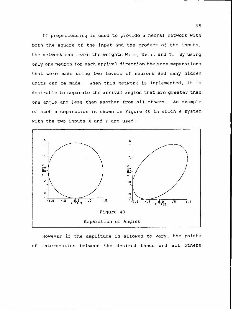
95

If preprocessing is used to provide a neural network with

both the square of the input and the product of the inputs,

the network can learn the weights Wx.i, W2, , and T. By using

only one neuron for each arrival direction the same separations

that were made using two levels of neurons and many hidden

units can be made. When this network is implemented, it is

desirable to separate the arrival angles that are greater than

one angle and less than another from all others. An example

of such a separation is shown in Figure 40 in which a system

with the two inputs X and Y are used.

.- In

- X- -I, -i ' 5 , .'5

Figure 40

Separation of Angles

However if the amplitude is allowed to vary, the points

of intersection between the desired bands and all others

96

increase. Therefore additional hidden units to separate

amplitude above or below specified amplitude thresholds are

required. Figure 41 shows an example.

m

.~~~ ~5 1.0 -. ~ . ~

Figure 41

Separation of Angles and Amplitudes

4.10 Results of Beaniformer with Nonlinear Inputs

To define the area shown in Figure 41 four neurons can be

used to define points within the two curves. An example of

the results made with 4 hidden units and 10, and 20 inputs and

amplitudes ranges of 0.5 to 1.0 and .5 to 2.0 are shown in

Figures 42 through 45. In these simulations that use 20 input

sensors a two dimensional beamformer is used. This beamformer

had 10 sensors in one line and 10 sensors in a line perpendicular

to it.

This method provides superior results to the methods which

97

use only linear inputs. It also requires fewer neurons.

Multiplying and squaring inputs is a reasonable modification

to make, since the multiplication function is required when

ANNs are implemented. Those simulations that are derived from

the exact formula for the input will be referred to as "exact"

solutions.

A compromise between these two methods can also be

demonstrated. By using linear inputs and squared inputs

elliptical patterns which closely resemble the exact solution

can be realized. An example of the same four trials tested

with the exact solution are tested with the elliptical network

in Figures 46 through 49. These simulations will be referred

to as "elliptical" solutions. No noise was used in either the

elliptical or the exact simulations.

4.11 The Network's Dependency on Time

It was shown in Equation (4.7) that the networks using

linear inputs are dependent on time and must rely on subdividing

the network into segments or output averaging to provide

acceptable results. The networks with nonlinear inputs

described by Equation (4.15) demonstrate that these networks

can be independent of time. However even though the network

can be expressed in a formula which is independent of time,

there is no guarantee that the solution learned by the network

will be completely independent of time. To demonstrate the

98

effect that time has on these networks two simulations are

presented using both linear and nonlinear inputs. Figures 50

and 51 present the same two simulations as were shown in Figures

36 and 42. These plots demonstrate that when the linear input

systems are used output averaging must be employed to improve

the systems response. Figure 50 represents one of the best

linear networks and Figure 51 represents one of worst exact

simulations.

99

ARRIVAL ANGLES 80.0 -90.0

0. 10. ~ 0 . 30. 40. to. do. )07 dIo. do. 120.ANGLE -DEGREES

SARRIVAL ANGLES 70.0 80.0

ANGLE -DEGREESSARRIVAL ANGLES 50.0 -70.0

0. 10. 0. Jo. 57. 0. 0. do.ANGLE DEGREES

SARRIVAL ANGLES 50.0 -60.0

T- - ------

0. - - ANGLE~~ DEGREES d. d. -,0

RARIJVAL HN6LES 40.0 - 0.

0. 10. 4'0 o. o. 50. 67 0. 0. -o'. I oo.P -'L DEGREES

OR~RIVRL ANGLES 30.0 '40.0

FtN GL E DFEREE

h AAIVA RNGLES 10.0 )0.0

0. 20. 30. '40. 60 s. 7 77 10NJ ~H1V ES .0 0.0ANCLE -DEGREES

ANGLE DEGREES

Figure 42

Exact Simulation; 10 Inputs; Amplitude Range .5-1.0

100

SARRIVAL ANGLES 80.0 - 90.0

9 10. 21) 3'0 4"ANGLE - DEGRES- 0 o I@*ARRIVAL AGE 00 8.

ANGLE - DEGRE -ES 10SARAIVAL ANGLES 60.0 -70.0

io. o. o. 4o. o. do. )a. do. d. 10ANGLE - DEGREES

~ARRIVAL ANGLES 50.0 - 60.0

ANGLE -DEGREES

~ ARIVAL ANGLES 40.0 -50.0

ai. . o . :. o. d. o. d. d. i.ANGLE -DEGREES

SARAIVAL ANGLES 30.0 40.0

1i i. Q, o. qo d. do. )a. do. do. ?00.ANGLE -DEGREES

~ARRIVAL ANGLES 20.0 -30.0

ANGLE !'bEGAEH-7 ARRIVAL ANGLES 10.0 -20.0

6; ~~ANL -. DEGAEESi --

' ARAIVAL ANGLES .0 - 10.0 NL ERH. a d- d' 1@o

ANGLE - DEGREES a @ D' 'o

Figure 43

Exact Simulation; 20 Inputs; Amplitude Range .5-1.

101

ARRIVAL ANGLES 80.0 -90.0

ED

0. 10. 20. 30. 40. R.. . . 130.ANGLE D EGREES

HHfRAIVAL ANGLESC 70.- 80.0

.

. 10. )0. 0. 40. . 60. )0. do. do. 100.

SARRIVAL HNGLES 80.0 -70.0

0. J-. 0.~ . 400. q@ go o. do. do. ?Mo.ANGLE - bEGREE5

SARAIVAL ANGLES 50.0 - 60.0

I. 10. . 40. 40. 5. . . 0. do. 00o.ANGLE - DEGREES

_J ffHIVRL HNGLES 40.0 bO~.0

10. 10 40. 0. 0. 0. 0. 0. IM0

9RRIRL %GL5 -3.2 z~zANCLE bfQEAE5

P AR1AL ANGLES 20.0 3 0.@0 N IE E R E

10. Jo. 30. 40. o. 60. )o o do. '100.ANGLE DEGREES

~ RAIVA. ANGLES 10.0 3 0.0

0. 0. 0 40 . 0 o. . do. do. M0.ANGLE D EGREES

HH ARI VAL P'NLLES 0.0 1 0.0

~o. ~ o ~0 40 ~ o ?~0. o do. do. '120.ANGLE b EGREES

Figure 44

Exact Simulation; 10 Inputs; Amplitude Range .5 to 2.

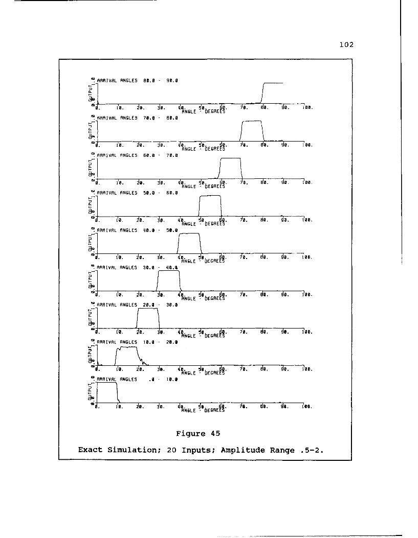
102

ARAIVAL ANGLES 80.0 -90.0

ANGLE - OEGRA E* ARHRIVAL ANGLES 70.0 8 0.0

ANGLE - EGRE ESSARRIVAL ANGLES 60.0 -70.0

L.I0 a.d. 40. qo. do. h. do. do. ?00.ANGLE -DEGREES

ARRIVAL ANGLES 50.0 - 60.0

LI o.~. Ia4. o o.Iao . d o o 0.

ANGLE- GESSARRIVAL ANGLES 40.0 5 0.0

ANL1.FRES to o o. 'o o.a.~ . do. do. 1100.

ANGLE - GRE SSARRIVAL ANGLES 20.0 -30.0

9I fa0. Ia. 0a. 40. q8. 2 ). do. do. 'oo.ANGLE - DEGREKL

'! ARRIVAL ANGLES 10.0 - 20.0

ANGLE - DEGREK '@ 'a

'!ARRIVAL ANGLES .0 - 10.0

. o ... .o .0 ..... ... o d . t

ANGLE - DEGREK )@ d' @

Figure 45

Exact Simulation; 20 Inputs; Amplitude Range .5-2.

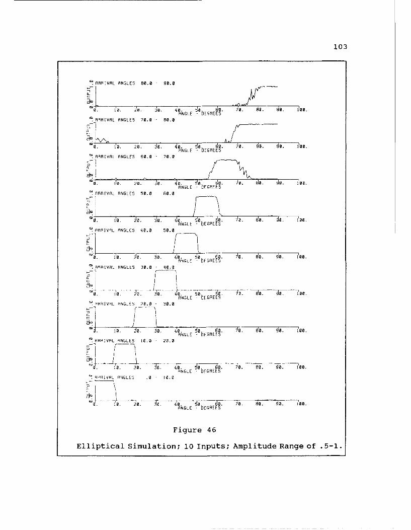
103

ARRIVAL ANGLES 80.0 90.0

0. 10. 2-0- . 30.. i dO. E o. do. do. i,1.S a.,,~ ,,O - ANG( E - DEGREES

ARRIVAL ANGLES 70.@ 80.0

VA ANE 0 .0 70.). do. d@.ANGLE DEGREES

. ARRIVAL ANGLES 60.0 - 70.0

ANGLE DEGREES

.ARRIVAL ANGLS 5.0 60.0

1-.'o 0. Jo. 40q o d E . o do. do. 'oo.ANGLE DEGREES

.HRRIVAL ANGLES 40.0 - 50.0

so.J - i'. o 40. o. o. o. do. do. 1'0.

ANGLE DEGREESARRIVAL ANGLES 30.0 410.

. .o. . 57. --7. )o. do. -2. 10e.ANGLE DEGREES

'~ARRIVAL ANGLES 20.0 -30.0

10. jo. jo. o. 0o 0o . d. o o.

ANGLE -DEGREES

H RRIVRL AN6LES 10.0 - 20.0

ANGLE OFDGREES

HHH1VAL ANGLES .0 10.0

0. 10. ) . do. -do. ,30.AGE-DEGREES

Figure 46

Elliptical Simulation; 10 Inputs; Amplitude Range of .5-1.

104

6ARPIVAL ANGLES 80.0 - 90.0

10.RIVAL.ANGLES0. .. 100.

SARRIVAL ANGLES 70.0 7 0.0

SARRIVAL ANGLES n0.@ - 00@ NL -@EA

:AAAIWRL71LES5E0 60. o do. '100o.

ANGLE EM DEGEE

A RRVA ANLS 4.I o

3

i.To. ~. do.4. o . h0. do. do. ?00o.ANGLE - EGREE S

~AAAIVAL ANGLES 20.0 3 0.0

-1

im0.~ . I@. 40. di do. . do. do. 10ei.ANGLE - EGREES

_RARIVAL ANGLES 10.0 - 2&0.0

C1

Q0. do. do o. d. o t0. 1'. ~ 0 ~ 0. ANGLE - bEGREES

'!-ARRIVAL ANGLES 2.0 1 0.0

a-.-I

CO. a i . o ~ . d. .~. do. d. toANGLE - EGREES

Ellitial ANLSimltos 10. Inus Amliue.0-.

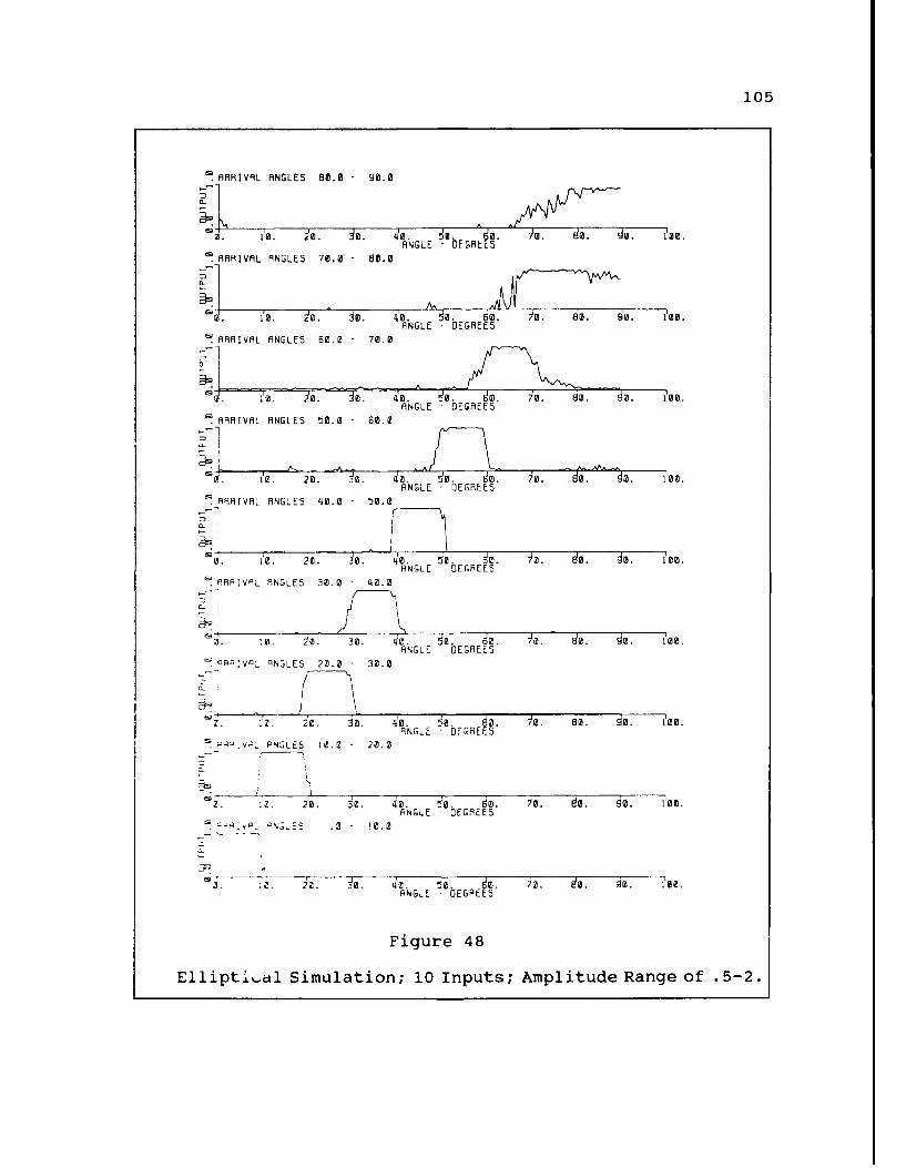
105

ARRIVAL ANGLES 80.0 -90.0

ANGLE - DEGRE SSARRIVAL ANGLES 70.0 80.0

So o. M. do. so. ioANGLE - DEGREES

SARRIVAL ANGLES 60.2 - 70.0

20~ 0 d.o. do. 1o.ANGLE -DEGREES

.JARRIVAL ANGLES 50.0 -60.0

ANGL - DEGREE

0 d.^ 4'0 do. do. )0. do. dO. 11oo.ANGLE - DEGREES

PRAAIVAL ANGLES 30.0 - 4Z.0

ANGLE b EGREE'SP ARRIVP ANGLES 30.0 2.

0. 3 . 1 19 E l u9 ES

o. 0. iz. 30. 40. t50. SdO.* 0. doa. de. 1,oo.ANGLE DERE

~~RAVAFiur ANLS2.8-3.

Elit0 a iuaio;1 nus mliueRneo 52

106

~ARRIVAL ANGLES 80.0 - go.0

ANGLE -DEGREESARRIVAL ANLE 7 500.0

ARRVHLANGES 0. 7 0.

ANGLE O EGRE ESARRIVAL ANGLES 60.0 - 7.

1q. 5. T.4.-. . Ao do. 100.ANGLE -DGES

~ARRIVAL ANGLES 40.0 5 0.0

10. 0.o. 40. ?.020 . . 10.ANL ERE

ARRIVAL ANGLES 30.0 - 0.0

9. 1. 'M- A0 ~ . . d. )I. die do. 100.ANGLE -DEGREE

ARRIVAL ANGLES 10.0 2 0.0

10.~ o ~ 0 4. ~ . o. o. do. do. 'I@@.ANGLE - DEGREES

ARRIVAL ANGLES 2.0 1 0.0

i'o. o AID. 40o. N EGR Qo . do. d. io

ANgLe 49GEE

ElAiVial ANLSiuaon 10. Inus 2mliue.0e.52

107

ARRIVAL ANGLES 80.0 - 90.0

4"' do. Ioo, 0. io .j 30 0GER .d. 40. d. do. {00.

ANGLE - DEGREES'2ARRIVAL ANGLES 70.0 - 80.0

1o. 10. )WGL[ " do. 4. do. do. ''oo.- DEGREES

ARRIVAL ANGLES 50.0 - 70.0

ii 10 0.4 0. 0o go. )0. do. do. 10ANGLE DEGREES

ARRIVAL ANGLES 50.0 - 60.0

&1. qo. do. 40 do do 00o do 10.ANGLE - DEGREES

ARRIVAL ANGLES 40.0 - 50.0

10o.- 0. 0. 10. d, o 0o. . 100.-NGL - DEGREES

ARIVAL ANGLES 30.0 - 40.0

.T - -- 0. 40. o. do. o. do . do.i o'o.

ANGLE DEGREESARRIVAL ANGLES 20.0 - 30.0

iA I ~vANGLE DEGREES

ARRIVAL ANGLES 10.0 - 20.0

10 .o. do. 4.. do. do. 100.NGLE -DEGREE5

ARRIVAL ANGLES .0 10.0

)0 J. 0 IcAN A/,/

10. 4 . do. 40. do. do. ioo.ANGLE -DEGREES

Figure 50

Simulation with Linear Inputs

108

SARRIVAL ANGLES 80.0 90.0

1@. 20. 30. 40. )o 0 . do. 90. '1@@.ANGLE b EGREES

ARRIVAL ANGLES 60.0 - 70.0

do. do lmeANGLE DEGREES

SARRIVAL ANGLES 60.0 7 0.0

do 0~. do. do. lea.ANGLE -DEGREES

'!HARRIVAL ANGLES 40.0 50.0

ia. it. do Ic

ARRIVAL ANGLES 30.0 -40.0AGE-DGRS

ANGLE DEGAESSAAAIVAL ANGLES 20.0 -30.0

~ J. o )a~. 30. )0 s d.~ . do. do. 'lee.ANGLE -DEGRE E

'!AHAIVAL ANGLES 10.0 - 20.0

ANGLE DEGREE

-ARIVAL ANGLES .0 10.2

it. qv. . ~o. do. do. Illg.

Figure 51

Simulation with Nonlinear Inputs

Chapter 5

Model of Wideband Beamformer

5.1 Design of Wideband Beamformer

When designing a wideband beamformer more information must

be input into the network in order to determine direction

correctly. This can be done in one of two ways. Temporal

data can be saved and applied to another dimension of neurons

in the network, or a two dimensional array of sensors can be

used. The choice may depend on the price of sensors versus

the price of analog circuits to store analog outputs. For

this discussion the two dimensional beamformer array will be

used. An example of a typical array is shown in Figure 52.

To determine direction from this array it can be viewed

as two arrays, one in each direction. It was shown in Chapter

3 that a wideband beamformer is a function of both (A and 0.

Since two variables are involved two linearly independent

equations in the two unknowns are required.

5.2 Mathematical Analysis of Wideband Beamformer

An analysis of a wideband beamformer is similar to that

of a narrowband beamformer. For the units in one dimension

109

110

HORIZONTAL NARROWBANO BEAMFORMERr- - - - -----------.

--I -_J - - - - - - - -

VERTZCAL 0NARROWBANDREAMFORME WIDEBAND BEAMFORMER

Figure 52

Two Dimensional Beamformer

the beamformer is the same as before.

1', =A. SIN(wt +ia) ( .)

2ndSIN(O) 2Tia= and N-x it

Where C is the propagation \elocit/.

In the direction perpendicular to this line the formula will

be

I'=A . SIN(ut+j) (.2)

2ndCOS(0)

As was shown in Equation 4.3 the equations for Vo and Vx can

be combined to form an equation that is independent of time.

1 -2 1 L0 I C+l 1 2 SIN (g ,)=000 2 I (5 .3 )

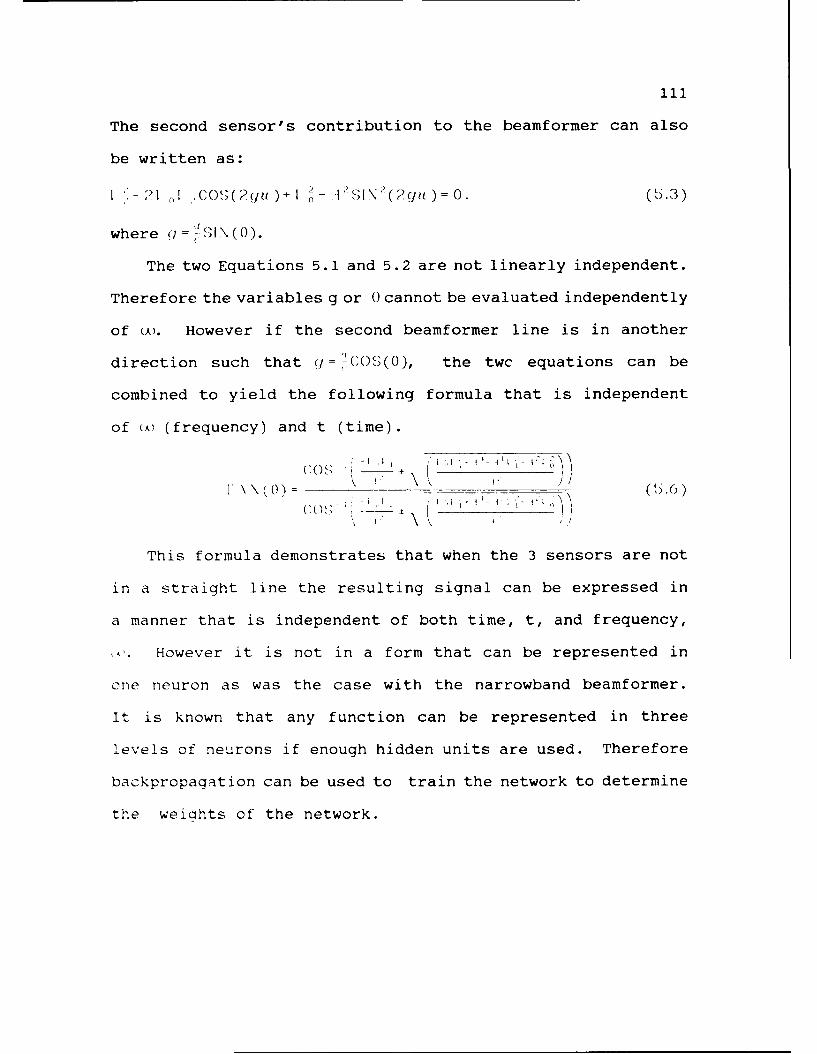
il1

The second sensor's contribution to the beamformer can also

be written as:

I - ,Cw;(2Yt)+I -. I "SI\ '(2m )=0. (5.3)

where (/=-I3\(0).

The two Equations 5.1 and 5.2 are not linearly independent.

Therefore the variables g or 0 cannot be evaluated independently

of (A). However if the second beamformer line is in another

direction such that (/=1( OS(0), the twc equations can be

combined to yield the following formula that is independent

of coQ (frequency) and t (time).

( j '- -1L - __

v (0) = - \ ,. \ ,. (S.)(' , - --- i ,,

This formula demonstrates that when the 3 sensors are not

in a straight line the resulting signal can be expressed in

a manner that is independent of both time, t, and frequency,

*,. However it is not in a form that can be represented in

one neuron as was the case with the narrowband beamformer.

It is known that any function can be represented in three

levels of neurons if enough hidden units are used. Therefore

backpropagation can be used to train the network to determine

the weights of the network.

112

5.3 Wideband Beanformers Using Backpropagation

Wideband Beamformers can be trained in several ways. Just

as with the narrowband beamformer these networks can be trained

by using the Delta Rule where the output of each level is

known. However unlike the narrow band beamformer the

appropriate values for the hidden units are not easy to

approximate. Mathematical calculations of the weight would

also be very difficult. This makes backpropagation the best

choice for training the network.

5.4 Results of Beamformers Trained with Backpropagation

Several sets of plots are presented in which Backpropagation

was used to train the network. The backpropagation required

over 60,000 iterations of training.

These plots are shown in Figures 53 through 61. In these

simulations three levels of perceptrons were used to form the

network. The simulations are made in sets of three to provide

an example of linear, exact and elliptical networks. These

sets of simulations are performed for networks with three

hidden units in each level (3x3) , 6x6 hidden units, and 10xlO

hidden units. These simulations indicate that linear networks

actually outperform the elliptical and exact networks. The

nonlinear inputs helped when simple narrowband cases were used,

but as the complexity of the input signal increased the linear

model proved to be the best. The advantage of using more

113

hidden units is also demonstrated. A comparison between these

three types of networks and the number of hidden units is shown

in Table 5.

Network Linear Exact EllipticalHidden Network Network NetworkUnits % Correct % Correct % Correct

3x3 91.87 81.08 80.966x6 94.29 93.40 87.121Oxl0 96.62 96.02 96.04

Table 5

Comparison of Wideband Beamformer Networks

All of the previous plots were made using a single frequency

component that was allowed to vary over a wideband as the

system was trained. To better demonstrate the networks wideband

abilities simulations were made in which two frequency

components of random amplitude were allowed to vary as the

network was trained. After training, simulations were made

in which 1, 2, and 7 frequency components were used to determine

whether the network was sensitive to the spectra of the waveform.

These simulations are shown in Figures 62 through 64. These

plots demonstrate that the network is sensitive to phase and

not the spectra of the waveform.

114

ARRIEVAL ANGLES 80.2 - 0.

0-

ANGLE - DEGREESARRIVA9L 19GE 00 6.

lo. ~~ANGLE - DEGRE95 doES' LeSARRIVAL ANGLES 60.0 0.

ANGLE - DEGREESSARRIVAL ANGLES 50. - 6.

a_

.k.jA A A

ANGLE - DEGREESSARRIVAL ANGLES 0.0A 50.

ANGLE - DbEGREES

-ARRIVAL ANGLES 30.0 4 0.eJ 0 .- A

ANGLE -DEGREES

~ARRIVAL ANGLES 20.2 3 0.0

10. q41. 'bEGRE S o. doSARRIVAL ANGLES 1.0 2 0.0

a-

~0. 0. do. r40. 01. 0 . d d. 10

Figure 53

Linear Wideband ANN, 3x3 Hidden Units

115

SARRIVAL ANGLES 80.0 - 90.0

-A t\ AA0. 10 0. a. 's0 q@ di. ho. do. do. 10.

ANGLE - DEGREES

R.fHIVML ANGLES 7 -. 70.0

0. 10. 20. Ia 0d. do). ho. Fe. o'. I a a.AINGLE b EGREES

R2 RRIVAL RNGLE56.0-70

* 1. ~ 1@d. 40 o .~. do. do. 'oM.

'~ARRIVAL ANGLES 50.0 - 60.0

* 1. o. o. '~o d. d. o. do. do. 1,00.

'!RRHIVAL ANGLES 40.0 -50.0

RRRIYAL RNGLES 3%.% 4. d . ~ . d. d. 10

a-

MARRIA ANGLES.. 20.0-'-30.0

20. Ia. qo. qO. do do. do. to20.ANGLE -DEGREES

ARRIVAL ANGLES 20.0 2 0.0

7T 7 ~ . d. 40. do. do. )M. do. do. 10@@.ANGLE - DEGREES

SARRIVAL ANGLES 0.0 1 0.0

~d. to. )a. Io@ o o. .~. do. do. ioo0.ANGLE - DEGREES

Figure 54

Exact Wideband ANN, 3x3 Hidden Units

116

ARRIVAL ANGLES 80.0 - 90.0

LJAV

. I0. i0. .0 0. L d R ES- . i0. do. do. I la.ANGLE A A L EG.EES

ARRIVAL ANGLES 60.0 7.0

,A - A. 10. do. 0.' 40. ao. do. 0. do. do. 100.

ANGLE DEGREESARRIVAL ANGLES 50.0 70.0

A A A . A(S ' .o .. do. a. do. 1o . '0 .

ANGLE DEGREESARRIVAL RNGLES 50.0 - 50.0

0 . q@ . do. )m. do. do. 'o.

ANGLE DEGREESARRIVAL ANGLES 40.0 - @.@

.d. J I. do. . 100.

ANGLE DEGREESARRIVAL ANGLES 0.0 - 30.

C9 . 0 . Ia.. )a. d . do . 1', 0.ANGLE - EGREES

SARRIVAL ANGLES 20.0 3 0.0

Ellptc. deA AA A A AUi

qo. A. Ia 4 . do. 9. do. do. I'oo.ANGLE -DEGREE S

SARRIVAL ANGLES 1.0 - 10.0

0. it. 0a. 40. do. . . 0o. 100.

Figure 55

Elliptical Wideband ANN, 3x3 Hidden Units

117

ARRIVAL ANGLES 80.0 90.0

C0

.- AA A A A AA. .10. 40.. 0. do. do. i0o.

ANGLE - DEGREES

ARRIVAL ANGLES 70.0 80.0

. 0 0. o. 0. . . do. 130

ANGLE - DEGREES

ARRIVRL ANGLES 60.0 70.0

A.A A A A

0. o. lo. W 2 o a o o 100.

{0. $e. 0. ANGLE -8. DEGREESO- . . . {0

SARRIVAL ANGLES 50. 60.0

. t. . .do. . .

ANGLE - DEGREES

SARRIVAL ANGLES 30.0 50.

10". 0. Ia. 8. do. )o. 0o. o. i@o.

ANGLE - EGREES.-ARRIVALANGL-ES 30.0 2 0.0

ANGLE DEGREES

SARRIVAL ANGLES 2.0 3 0.0

0. ~ .~ . . 40. 0". do. 0o. do. do. 1,00.

ANGLE DEGREES

ARRIVALFgur 56LS100 2.

Linea WidbandANN, x6 HddenUnit

118

ARRIVAL ANGLES 80.0 - 90.0

3! A A-A

ANGLE - EGREKE

ARRIVAL ANGLES 70.0 - 0.0

" ARRIVAL ANGLES 60.0 -70.0

i'o ~ . ~ . o.do. do. --- , a a.ANGLE DEGREES

~AR81VAL ANGLES 50.0 - 60.0

CL

ANGLE - DEGREES

~ARRIVAL ANGLES 4~0.@ 50.0

/A--A A A AA AM&~

19. 0'. A o t. d di.~ do. do. 100o.ANGLE - DEGREES

R2ARIA NGLES 20.0 4%3.%

ANGLE -D EGREE

~ARRIVAL ANGLES 20.0 - 0.0

ANGLE l'bEGRES. )0' do. d. IS'.

'!ARRIVLAL E~S 10. 20.0 AA A10

9. I'. it e. 4. dOb GRHS )M d ' d@ .ANGLE -DGE

Figure 57

Exact Wideband ANN, 6X6 Hidden Units

119

~ARRIVAL ANGLES 80.0 - 90.0

A . I A

0. 1. 20 30. 40. 0. d o. )@. d. d. 10ANGLE - DEGREES

ARRIVAL ANGULES 60.0 0.

A Ao. .A A o. d. )o. do. do. 1100.

ANGLE - DEGREESSARRIVAL ANGLES 60.0 6 0.0

MMARIVAL ANGLES 40.0 - 6.0

ANGLE - EGREE5

R ARIVAL ANGLES 30.0 9 0.0

2,

10. 50. T. )0o .Ado 100.

AIRRIVAL ANGLES 20.0 40.0

a-T

ANGLE - DEGREES

10. '40. o. - o. 0o. 100.

~ARAIVAL ANGLES 2.0 - 30.0

1 o. JO. doVV A. ).~ do. do. 1020.ANGLE - DEGREES

~~~~F g r 58IA AGE .0-2.

Elitia 2ie n AN, x6Hide Uit

120

SARRIVAL ANGLES 80.0 - 90.0

AAI.'@. 20. Jo. 40. 0. do. )@. do . do. 1,00.

ANGLE b EGREESSARRIVAL ANGLES 70e 80.0

I1

~ :~ . t.~ . do. 9w-o. d. (-.aooANGLE -DEGREES

'. ARRIVAL ANGLES 60.@ 6 0.0

(1

~. o.~o ~. 'o.~o d. .do. do. 10ANGLE D EGAEES

SARRIVAL ANGLES 40.0 5 0.0

-d. o ~.~ .~o o o do. ;0. 100.ANGLE - EGREES

*ARRIVAL ANGLES 30.0 4 0.0

C1

ANGLE -bEGRE ES~ARRIVA9L AN~GLES 20.@ 3 0.0

Q. A . Jo 1@.- 4o. lbE do. )M' do. o.' 100.ANGLE - ERES

'J ARRIVAL ANGLES 20.0 30.0

1@ 0.~ . 411. bEGRES )W. d@. lee10.

'!ARRIVAL ANGLES 1.0 - 20.0

7

----- - A A .o-- i'o2 0. 1@. 40. do. do. )m. . do. Me.

ANGLE - DEGREES

ARRIVALFgur ANLS .091.

LierWdbndAN 0l Hde nt

121

~ARRIVAL ANGLES 80.0 90g.0

7~T o. o. M o. d. )OA o o 'oANGLE -DEGREES

~ARRIVAL ANGLES 70.0 -80.0

Jio.10 d. '0o d. go o. do. I'M.

ANGLE -DEGREES

~ARRIVAL ANGLES 60.0 - 70.0

9 10. D. A0. 40. do. (a. a.AINGLE -ODEGREES51

~ARRIVAL ANGLES 40.0 - 50.0

Qi 10. do. 40. 0 o d.~ . do. Do. ioo.AINGLE -ODFGREES

~ARRIVAL ANGLES 30.0 5 0.0

a. IJo A o - 0. 40.~ E . -0 ). do. do. 'leSARRIVAL ANGLES 20.Z - Z It.

10 d. 0. 40 o. 0. ho. do. do. 100.RINGLE b EGREES

~ARRIVAL ANGLES 10.0 20.0

ANGLE - EGREES'- RRIVAL ANGLES 1.0 20.0

Q. 0 . do. 140. 0 o do. do. 1 00.

AGE-DEGREE S

Figure 60

Exact Wideband ANN, lOxiG Hidden Units

122

SARRIVAL ANGLES 80.0 - 90.0

-1do

a-- A,

Jo . do o 4. d. 7 o0. 10 ~0. do. NGLE - EGREES

'!ARRIVAL ANGLES 71.0 - 70.0

A A l

ANGLE -DEGREES

SARRIVAL ANGLES 50.0 6 0.0

'ANGL - EGREES

~ARRIVAL ANGLES 50.0 506.0

A 1 AA* A A

ANG.LE-DERS6ARRIVAL ANGLES '4b.0 13 0.0

ANGLE - DEGREES'!-RRIV'AL ANGLES 10.0 - 20.0

10. ~ ~ AGL -o do o O do. . do. d. 10

6ARRIVAL ANGLES 2.0 - 0.0

to.~do M. o.~. oANGLE - DEGREES

Elitia RRIVALd ANGLE 10.0 Hide Unit0

123

ARRIVAL ANGLES 80.0 - 90.0

,-A&,, A A A-A A \ AlN- J A UI0. 1. 2 0. J0 4. 50 d . . 0.

ANGLE - DEGREES

PARRIVAL ANGLES 70.0 - 80.0

0. 10. 70. 30. L. 0' d. h0. do. do. 100.ANGLE• DEGREES

ARRIVAL ANGLES 60.0 - 70.0

ANGLE OEGREESARRIVAL ANGLES 50.0 6.0

9NGLE - a';REES

SRAIVAL NGLE5 40.0 10.0

oz . 0. 60. loo..€- "";EE,

'0. no.R 60.! go.. -1

.NS 100.

- - ^ -,

2. :0. 2 . 3 . qZ. 0. 52. 72. 82. 90. 100.

. 3C. . 0o. S. 62. 7o. 80. go. M00.

-- A 'V\ AA~ A1

., 0, 22z. 1z. . to. 6 . '0. 82. 90. :20.r , -E _',-,qE

Figure 62

Linear Wideband ANN, 1 Frequency Component

124

SARRIVAL ANGLES 82.2 90.0

ANGLE - EGREES

ARRIVAL ANLE 7 6.2.0

~ARRIVAL ANGLES 60.0 70.0

i0e.ANGLE - EGREES*

SARRIVAL ANGLES 40.0 50A.0

2.. 4. 70 2) 100.

ARRIVAL ANGLES 3Z.t 4Z.

2s.-TM 9. * . toO.A'NGLE -ODEGREES05

SARRIVAL ANGLES 20.2 30.2

ARRIVAL ANGLES 10.0 20.2

4~ do.. rANGLE DEGREES

i ilHIV'IL ANGLES .2 10.2

0.

a~. 1 ).o. 0. & ~ W do. do. too.ANGLE DEGREES

Figure 63

Linear Wideband ANN, 2 Frequency Components

125

ARPiVAL ANGLES 80.0 - 90.0

0 10. 2. o. 40 0. do. )0. do. .o 100.ANGLE -DEGREES

ARRIVAL ANGLES 70.0 80.0

i . to. _o. o. 40. do o. ~o. d. do oo.ANGLE - DEGREES

ARRIVAL ANGLES 60.0 70.0

.O. Jo. Jo. 4 o. .o. do. do. i00.ANGLE - DEGREES

ARRIVAL ANGLES 50.0 60.0

'. to. Jo. do. i o. d:. o. do. 10. .10.ANGLE - DEGRFEb

'!ARRIVAL ANGi ES 40.0 50.0

'.. 0. 0. 0. 0o. 0. 1..ANGLE - FEGREE5

ARRIVAL ANGLE5 30.0 - .0

0-i

V. 10. 0. A. 40. O o. 7o0 do. do. 1oo.

ANGLE DEEREES

ARRIV9L ANGLES 20.0 30.0

J. a 40. 0. . ... 0. 100.ANGLE - DFGREES

A RRIVAL ANGLES 10.0 20.0

. 70. ANGLE 0 0FGREE5 0. 0. 0. 100.

HAH IVAL ANFL E5 .0 i1.0

..0. 20. 0. 40. q@. do. )o. do. do. 10o.ANGLE DEGREES

Figure 64

Linear Wideband ANN, 7 Frequency Components

Chapter 6

Empirical Demonstration and

Comparison of FFT and ANN Beamformers

6.1 Seismic Test Description

To demonszzate how the direction of arrival of a signal

can be determined from a trained ANN, the following experiment

was performed. A seismic array was arranged in a three

dimensional pattern with twelve geophones. A movable signal

source was used to transmit a wideband wave from three different

directions. The received signals were corrupted by the presence

of a crane at a fixed position in the vicinity of the geophones.

In addition to this mechanical noise, 60 HZ electrical noise

also corrupted the data. Several tests in which the signal

source was moved to different ranges in the three directions

were recorded and digitized. A diagram of the test is shown

in Figure 65.

The task for the neural network to perform is one of

determining the direction of the signal while rejecting the

mechanical and electrical noise in the system. One of the

advantages which neural networks have over conventional signal

126

127

3-D SENSOR LOCATION

I"• CRAN

I %

%% *

S S

I S

I S

I S

Figure 65

Seismic Test Diagram

128

processing is the small amount of information required to

train the network. For example the exact directions are not

known but are labeled A, B, C for convenience. The array's

configuration is known to be three dimensional but the order

and exact location of the gages need not be known. The

calibration of the gages in inches per second is known to be

sufficient to acquire the signal of interest but the output

is passed through an automatic gain control routine to provide

the network with an input with a narrow amplitude range. The

exact output level of the AGC is not known or required. The

exact frequency spectra of the noise source and signal source

are not known. However the data was digitized at a sampling

rate greater than twice the bandwidth of the velocity gages

used to acquire the data. This prevents aliasing of the time

sampled data. Since the frequency spectra is not known, it

was assumed to be a wideband signal. In order to prevent

aliasing in the spatial dimension the spacing of some of the

geophones were placed closer than one half of the minimum

wavelength to be received. The minimum wavelength is equal

to the propagation velocity divided by the maximum frequency

that the gages can receive. With only a brief (20 seconds)

time history of the output of the geophones the network can

be trained to recognize the direction of the desired signal

and ignore all other interference. A time history plot of the

129

data used to train the network is shown in Appendix II. These

plots show an example of one second of data at all three

directions and two different ranges.

6.2 Results of Seismic Test

Once the network was trained samples of both the time

signals used to train the network and the other recorded signals

were processed through the network. The results are shown in

Figures 66-71. Figure 66 is a simulation in which the input

data was the same data that was used to train the network.

This data was 20 seconds in duration and represented the data

closest to the geophones. In Figure 67 another sample of data

recorded at the same range was used for the input to the

simulation. In Figure 68 through 71 samples of data from other

ranges were used for the simulations. Each of the plots

presents the three network outputs as a function of time.

Ideally an output of one represents the presence of a signal

from the direction associated with that output, and a zero

represents the absence of a signal. Since only one signal was

present in each of the tests, one output should predominate

the other two.

These plots indicate that the response is much better for

the data that trained the network than for other data sets.

The expected reason for this is that the data used to train

the network was not very representative of the data in the

130

other data sets. The spectral characteristics of the data can

easily change with distance or with the intermittent operation

of the crane. It was demonstrated in Chapter 5 that when a

wideband signal is used to train the network it will be able

to recognize signals with different spectra. It is however

imperative that training signals be wideband signals that

encompass all the frequencies to be received by the ANN.

The output of the ANN was analyzed as if the output level

was connected in a winner-take-all configuration. In such a

configuration only the output with the highest amplitude is

asserted. The results can then be compared with the known

direction to determine the percent error in the simulation.

Thirteen segments of data were analyzed. The error for each

of the thirteen segments is shown in Table 6.

It should be noted that the results ranged from very good

(0 % error) to rather bad (31 % error). The 0 % error occurred

when the training set was used as the input to the network.

The high errors however occurred at both ranges and at all

three angles. This indicated that range was not as an important

factor as were other temporal phenomena. This can be seen

rather clearly from Figure 69. It can be seen that during the

first twelve seconds the network functioned very well, but

something happened during the last eight seconds that alters

the networks result. This could easily have been a modification

131

TRAINED FOR DIRECTION C NETWORK C

~ . i ~12. 14. 1IS. 18. 2.

TRAINED FOR DIRECTION 8

-A-,

1~.1 0 40 .0~I ~ 2. 1. 17 7 T .TI ME -SEC

TRAINED FDR DIRECTION ANEWR A

NETWORK A

\J NETORK C

Figure 66

First Simulation with Training Data as Input

132

TRAINED FOR DIRECTION C

TRAINEDETOR AO IETO

4. . IN C 12 ' '. 18

TRAINED FOR DIRECTION R

NEWR

NETWORK C

STIM16tEC 1. I. 1. 8. .

TRAIFigur 67 IRCIO

First ~ ~ ~ ~ ~ ~ NTWR Si uai n wtAiia aa a n u

133

\..FA A ,4TV fRK 9- v

IA r,' 1 Nt 140A

-- -- --T r 0TIME 5FC

THFINE C FA DIREC TION 9

NE IWORK A

VV

NETWORK, C0 .0 -J .0 - 4 . . 1 0 . 1 2 .--4. . 7 6 e - .

TIME-SEC

Figure 68

First Simulation with Different Range of Data as Input

134

TRAINED FOR DIRECTION B

TIME-SEC

TAH[NEO FOS DIRECTION R

66. 1.0 4.6 d.0 d.0 N EC . I. 8 18.TIMESE

Figure 69

Second Simulation with Different Range Of Data as Input

135

RR NE2 IR UIR I@TN

P,

~VvV~f' A ANETWORK A

AAPA \WjVv/ v v'N\ V Vv

A-(IM

VV

A ,A v~\ A jI~ J NET WORK

TIME SE-

CPRIFigur 70 IEC O

Siuato wit Siilar Dat NETWORKut

136

TRAINEO FOR DIRECTION 8

/A~vv~f"' \/vAAf~\I~JVVNETWORK 8

NETWORK C

0. o L . 0 1@. 12. 14. I's. ,8. io.TIME-SEC

TRRINEO FOR DIRECTION A

S * o .. d, .0 14. 1'2. 14. 16. 1,8. Jo.TIME- SEC

Figure 71

Simulation with Different Range of Data as Input

137

Test and Direction Direction DirectionRange A B C

Test 1 0 % 0 % 0 % Training SetRange 1

Test 2 2 % 0 % 27 %Range 1

Test 3 31 % 1 % -

Range 2

Test 4 17% 10 %Range 2

Test 5 5 % -

Range 2

Test 6 3 % -

Range 2

Test 7 -0 %Range 3

Table 6

Percent Error in Seismic Test

in the operation of the crane that introduced a type of noise

into the system that was not present in the training set.

Another important characteristic to notice is that when the

signal is sent from direction A or C the distinction from the

most distant sensor, C or A, is almost perfect and very distinct.

This demonstrates that the three angles could be too close to

distinguish with the twelve sensors. The overall success rate

for simulations not in the training set was 90.4%. The success

rate for the training set was 100%.

138

The quality of performance of a neural network can best

be determined by the networks success with data not contained

in the training set. The success rate of 90.4% indicates

excellent performance for a system containing large amounts

of interference and noise. Correlated noise such as that

produced by the crane can cause particularly severe difficulties

since the network must be trained to process one signal while

ignoring another.

6.3 Comparisons between FFT Beamformers and ANN Beamformers

When comparing FFT beamformers and ANN beamformers several

major differences should be considered. These differences

are:

(1) FFT beamformers are programmed using DSP hardware and

programming languages, while ANN beamformers are taught using

modifiable artificial neurons and training algorithms. When

the mathematics and programming are simple as is the case with

the narrowband beamformer, the FFT method has an advantage.

However when the programming becomes more difficult and

trade-offs between design complexity and performance are to

be made an adaptive system such as ANNs offers advantages.

(2) FFT beamformers require considerably more hardware

than ANN beamformers, but since ANNs are trained, training

examples must be available for the system to use. Training

139

can require many iterations for even simple problems.

(3) The steered beams of the FFT beamformer are at arrival

angles determined by the formula 0Since the phases,

a, are spaced at equal increments due to the symmetry of the

FFT algorithm, the arrival angle beam wil. be at spacings that

are a function of the arcsin of these phases. ANNs, however,

can be trained to distinguish any band of angles from any

others.

(4) The FFT beamformer is a linear system. The FFT

beamformer accepts analog signals digitizes them, processes

them and produces analog output signals from a digital to

analog converter. As in all linear systems doubling or tripling

the input will double or triple the output. The property of

superposition will also assure that if two inputs signals are

applied, the output will be the sum of the outputs of the two

signals applied separately. ANNs however are not linear

systems. They accept analog inputs but have outputs that

approximate discrete digital levels.

(5) ANNs can be taught to ignore correlated interference

that may be present in the environment. FFT beamformers will

report correlated interference as a received signal.

(6) FFT beamformers provide an output that varies with

time. Since the information is returned to the time domain

in the last stage of the beamformer a time history is provided

to indicate both the direction of the wave and its signature

140

as well. The ANN beamformer provides only the directional

information.

There are also several similarities between the two

beamformers:

(1) The performance degrades as SNR is decreased.

(2) The performance is poorer for wideband signals

compared to narrowband signals.

(3) The performance can be improved by increasing the

number of sensors and the number of processing elements.

6.3.1 Simulation Comparisons of FFT and ANN Beamformers

In order to compare FFT and ANN beamformers the following

simulations were made:

(1) Narrowband beamformers were simulated. Both

beamfotmers used 9 beams. The FFT beams were at equal phase

angles and the ANN beams were at equal arrival angles. A

narrow amplitude band of .95 to 1.05 was used, and 18 sensors

were used. A simulation with no noise and one with a SNR of

7.78 db was made. 20 time samples for the FFT beamformer were

used and 20 samples were averaged with the ANN beamformer.

( A DFT was actually used since the number of samples was not

a power of 2.) The ANN beamformer used four neurons in an

elliptical network. The results are shown in Figure 72 through

75.

141

(2) Wideband beamformers were simulated. The FFT

beamformer used 3, 4, and 20 sub-arrays of 18 sensors each.

The ANN used multiple arrays in 2, 3, and 4 lines. Each line

contained 18 sensors. The spacing for each sub-array of the

FFT beamformer was tuned to a frequency half way between the

maximum and minimum frequencies for that array. The spacing

for each line of the ANN beamformer was set equal to one half

the wavelength of the highest frequency to be received. The

ANN beamformers were simulated using 20x5 hidden units in a

linear style network. Simulations with no noise and simulations

with SNRs of 7.78 db were made for both ANN and FFT beamformers.

A frequency range of 30 to 300 Hz was used. The results of

several of these simulations are shown in Figures 76-83.

In order to compare the results of the two beamformers the

outputs were evaluated by comparing their outputs to a specific

threshold. Outputs greater than the threshold were considered

true and outputs less that the threshold were considered false.

For the FFT beamformer a threshold of 0.5 (3 db) was used.

The ANN beamformer used 0.7 for the true threshold and 0.2 for

the false threshold. Twenty points were averaged on the ANN

beamformer to produce the average output. The absolute maximum

of the 20 sample time chip was used for the output of the FFT

beamformer.

142

SARRIVAL ANGLES 67.6 90.

ANGLE 1'bEGRE91.

SRARIVAL ANGLES 54.5 -67.6

~o. ~ o ~ m. do. 'l o d. Toc.ANGLE -DEGREES

ARRIVAL ANGLES 413.8 53.4

Jo. 40 .~. do. do 1,o I.

)a 'o .d. do. iwo.ANGLE -DEGREES

ARRIVAL ANGLES 246 - 42.7

0%

a. . 1o 0. 6D. qe. do. )'o. do. do. 1,20.ANGLE -DEGREES

ARRIVAL ANGLES 26.6 - 33.74

a . 'I Ia o do a do. do. 00I ANGLE b0EGREES

SARR1IVAIL ANGLES 11.2 - 15.6

io. o. o. 40. IdEGREM.- w do. d. iu

'ARRIVAL ANGLES 11.2 - 17.8

~J. ~ .ANGLE bEGRE'!.RRRIVAL ANGLES 4.0 103.2

1'o. A~1NGLE bEGRE~ w do. d. io

Figure 72

Narrowband DFT Beamformer; No Noise

143

SARRIVAL ANGLES 67.6 - 90.0

a-

I 10 h . , . do.ANGLE - DEGREES

*ARRIVAL ANGLES 54.5 - 67.6

i . . jo. -40 do do. )0I s. do. 70.ANLa ERE

*ARRIVAL ANGLES 43.0 - 53.4

ANGLE - DAEES

SARRIVAL ANGLES 34.6 -42.7

"w"

A NGLE -DEGREES

ARRIVAL ANGLES 26.3 - 33.7

ANGLE - DEGREESaARRIVAL ANGLES 18.6 -25.4

ANGLE -DEGREES

9 RRIVAL ANGLES 11.2 -17.8

ANGLE - DEGREES* M

SARRIVAL ANGLES 4. - 10.4

ANGLE b EGREES

Figure 73

Narrowband DFT Beamformer; Noise Level 1.0

144

ARRIVAL ANGLES 80.0 - 90.0

Joe~. jo. 'to do. do J o do. do. too.-- A~~NGLE -DGE

SARRIVAL ANGLES 70.0 - 80.0

-1-

aJ. mo Joo. 11. 470 . do. )0. do. do. '100.ANGLE -DEGREES

~ARRIVAL ANGLES 60.0 - 70.0

~ t. o. o.~o q@o do. o. do. do. 'le0.ANGLE -DEGREES

SARRIVAL ANGLES 50.0 -60.0

13

ED .'o . JIBo .. 0o. to.

ANGLE - EGREESARRIVAL AGE S% 4.

ANGLE - EGREK So~ARRIVAL ANGLES 20.0 3 '0.0

IJ 'o. )a. do Ef.t- d. o do. 90. leo.ANGLE b-EGREE

'!ARRIVAL ANGLES 20.0 2a3.0

C9 o. 10. . !o. E. d .ko do. do' 1 o 'ANGLE -DGEE

~~~~~Fgr ARIA7NLS400-2.

NarwadAN emome;N os

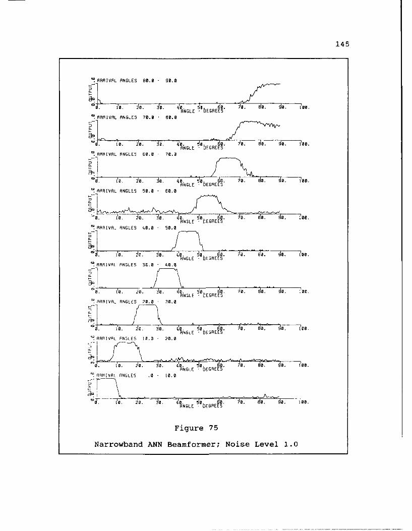
145

SARRIVAL ANGLES 80.0 90.2

ANGLE - DEGREES~ARRIVAL ANGLES 60.0 70B.3

ANGLE DERSARRIVAL ANGLES 50.0 - 60.0

aI

10. E 0ANGLE - DEGREES5

ARRIVAL ANGLES 30.W Q At.Q

0-

ANGLE - DEGREESARRIVAL ANGLES 20.0 3 0.0

ANGLE - DEGREESARRIIVAL ANGLES 10.0 20.

Q 1'o. )@. Jo. ANGLE - DEGREES I . lt

ARRIVAL ANGLES 2.0 - 30.0

0. . 0.d.o. do. 120.ANGLE - DEGREES

Figure 75

Narrowband ANN Beamformer; Noise Level 1.0

146

SARRIVAL ANGLES 67.6 - 90.0

ANGLE - DEGREES- ). d. d. t

ARARIVAL ANGLES 54.5 - 67.6

9s ARRVA ANLE 43.8 - m

ANGLE - EGAEES

n-*ARRIVAL ANGLES 436-20.8 0 . 40 . 0 . 0 . 1

* ANLES 6.3 3.7ANGLE -DEGRE ES

d .A. Ia. -4 1 q 0. )0 d d 4. ?m0ANGLE DEGRE S

SARRIVAL ANGLES 2.3 33.7

eg. 9. i2 o o . do. do. ioe.

-1RRIVAL ANGLES lbIr 2 5.4 AGE DERE

0IL

ag I'.4O o. q. q@. do. )w. do. TeO. 1 a0.ANGLE - EGREE S

' ARRIVAL ANGLES 11.2 10.e

10 0 o.q.d. o g do. do. coo.ANGLE - EGREES

ARRIVAL ANGLES .0 - 3.2

0.

ANGLE -DEGRE E

Figure 76

Wideband DFT Beamformer; 3 Sub-arrays; No Noise

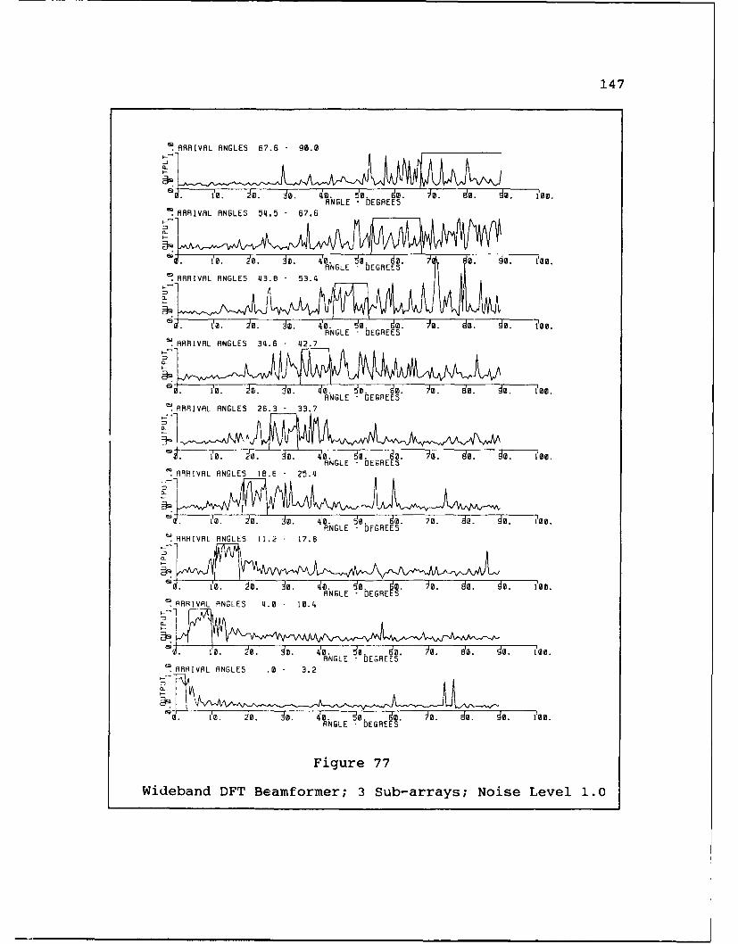
147

ARRIVAL ANGLES 67.6 - 90.0

ANGLE - EGREES~ ARRIVAL ANGLES 54.5 -67.6

a. 0'. 0.4 0 40. q. 0o. 0. . 0. 1 .ANGLE - DEGREES

'ARRIVAL ANGLES 431.8 -42.

a.T . -T. q, do. )Q. do. do. 1,00.ANGLE - DEGREES

ARI VAL ANGE 46 - 4.

ANGLE -DEGREES

ARRIVAL ANGLES 16.6 -25.4

do 0 ~o do d. o. do. do. 100.ANGLE - DbEGRES'

SARRIVAL ANGLES 11.2 17.8

do.o do. iooANGLE - DJEGREES

~ARRIVAL ANGLES 4.0 3 1.2

ANGLE - DIEGREES_

Figure 77

Wideband DFT Beamformer; 3 Sub-arrays; Noise Level 1.0

148

5! ARRIVAL ANGLES 67.6 - 90.0

tn II-

~ 0 0. Io. 40. 61. . do. do. 1,26.

SARRIVAL ANGLES 54.5 - 67.6

o. ANGLE 'bOEGR E o. d. d. i.SARRIVAL ANGLES 43.8 - 53.4

ad. J'. do O. 4. b0 o o die. do. oo0.ANGLE -DEGREES

ARRIVAL ANGLES 34.6 -42.7

ai. ea I@. I@. do. 8m d. I~a. do. do. IBM.ANGLE - EGREES

SARRIVAL -NGLE2 2e.3 33.7

~o~i'w do do 'o. o. o. o. o. do. eoo.ANGLE - EGAEES

ARRIVAL ANGLES 16.6 -25.q

~ 'o d. o 'o.~ '. do. )II do. I. I 0wo.ANGLE -DEGREES

-JARRIVAL ANGLES 11.2 - 17.8

5-I

ANGLE - EGRE SSARIAAIYL ANGLES 4.0 110.4

nIL

NGL. do . oo w a. . do. do. 100.

'!-ARRIVAL ANGLES .0 - 3.2

a-

ew. To. Ia. lbw.R hw o . do. do. Im.ANGLE - DGEL

Figure 78

Wideband DFT Beamformer; 4 Sub-arrays; No Noise

149

ARRIVAL ANGLES 67.6 -90.0

ANGLE -DEGREESARRIVAL ANGLES 43.8 536.4

0. t. g o 0 o o.~ . d. d. io.ANGLE -DEGREES

ARRIVAL ANGLES 343.6 425.7

d.

ANGLE -DEGREES

ARRIVAL ANGLES 2534. 33.7

a-

Q. ANGLE -DEGREES

ARRIVAL ANGLES 286 253.7

Q-

do. 40.do. )m. do. do. ?ea.ANGLE -DEGREES

~J. to. ~ o d 41~. do. do. H o. do. do. ioANGLE-DERS

SARRIVAL ANGLES 11.20 17.4

AINGLE - DEGRES' )' d a aM~AR RIVAL ANGLES 40-t.

ANGLE - DEGREES-

Figure 79

Wideband DFT Beamformer; 4 Sub-arrays; Noise Level 1.0

150

RIVH fiNGCS 8?.0 9@.?

II. 10. 20. 30. 40. W~ 5. 7. 2. 1? 7"?.'i E EG EF

P.N7Lf bEGFHE_5

10.lAR,: E0 . @ 76. 2I -

:0 30. 40. 6f,. a. 2P. (L r1GFE S

,!Pn~p H NG. ES 40. 50S.2

a. A. 23. 40. -5c. 5a 9?. JO 1. 12z.F-%StE (IE w 5*

9PFH[Vr'% RNI,. 5 32.0 40.?

M~ 5RI FSN~r 22.0 30.? I.Lf hGE

20. 30. 4@. 0). 2.6 . 2. I.f~ lf nrr S

LI 0 0. 30. 40. 30 . 2. 11: %,E blEAFEES

Figure 80

Wideband ANN Bearnformer; 2 Arrays; No Noise

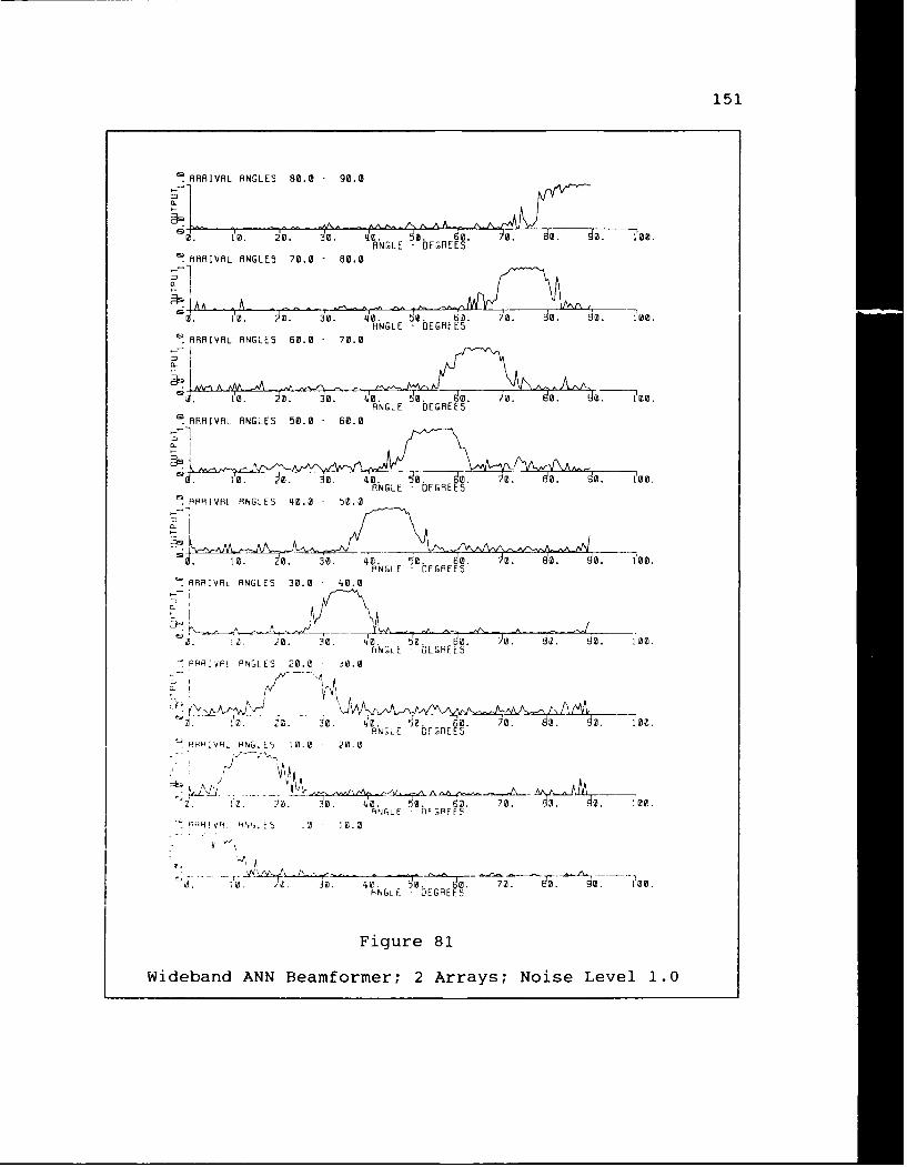
151

'! ARRIVAL ANGLES 80.0 - 90.0

Q. 10. 2Q) 30. leeS d. ). o o. io.ANGLE -DEGREES

ARRIVAL AGE 00 6.

0. 3. 0 0 bI0 . . d. O. 100o.ARRVALANGLE -DEGHEES

ARIA ANGLES 60.0 - 70.0

AA AAA -U. 100 . . 0. 401. q@. do. )0. do. Ia. Too

ANGLE -DEGREES

SARRIVAL ANGLES 50.0 -60.0

10 o JD rm 0 d. )0. do. 0o. 100.ANGLE - DGREES

H. ARIVAL ANGLES 40.0 - t0.0

10. 0. 310. 40. - 2. 80. 0M. 80. 0o. 100.ANGLE - DEGREES

RRIVAL ANGLES 30.0 - 40.0

-

0. 2 0. 3. 4.70 . 0. 50. . 100.ANGLE DE&REES

rRRfVFL ANG ES 20.0 jib. 0

A . 6.40. 50 0 0. o. go. 100.HNGE - DEGREES

Wiebn ANNL 0.0frr 22ray;Nos.Lvl0.

152

ARRIVAL ANGLES 8a.0 90.0

0. 10. 20. 30. 40. d. d.~ . 0 . 10ANGLE - DEGREES

ARRIVAL ANGLES 70.0 - 80.0

S.T . jo. 40. 0. . . . 0. 100.ANGLE DEGREES

ARRIVAL ANGLES 60.0 70.0

40.. . do. o0. 70. 80. do. i0o.ANGLE - DEGREES

ARRIV9L ANGLES 50.2 - 60.0

.i.".-- o .- 4. 0. 0.- 70. do. !a. 100.ANGLE DEGREES

ARRIVAL ANGLES 40.0 50.0

J. 40. ao d-O. 0 0 10ANGLE - DEGREES

ARIVAL ANGLES 30.Z 4%.Q

S1. o. d. o. d. do^ )o. do. do 100.ANGLE DEGREES

-ARRIVAL ANGLES 20.0 30.0

M1 AA AP' .

10., A0. do bEGodo do. 10.

ARRIVAL ANGLES It.M 20.0

ANGLE - DEGREE5ARRIVAL ANGLES .0 10.0

i0. q1 do ). do. do. 130.

ANGLE - OEGREES

Figure 82

Wideband ANN Beamformer; 3 Arrays; No Noise

153

p2 RRIVlL ANGLES 80.0 90.0

6. 10. 20. 30. 40. t . )o. do d .. ,ZANGLE - DEGRSEES

.-9M3VHL HNGLE5 70.0 aO8.0

0. 1. 2Z. . 40. 0. do. 0. do. do. 'lee.

Fi~RRVRL f9NGL5 60.0 70.0

30 e 410 t. 3. 70B. do.a - . 120.

ANCE GEREESRPRIAL FNGES 5.2 0.0

(Z. 10 .0 . 4 . 6z. 70. 80. 90. 00e.

3N FGREES

0. :z. 2z. 30. Z0. 50. S2 )o. 80. go. :00.

'N TSE !F-PEE--

0. . 22. 303. 4Z. !5o. 50. 70. 90. 90. :00.

80. I' iz

;.:0 0. j2 0 2 . 4 . 0. 12. 620 2 i* 20.

Figure 83

Wideband ANN Beamformer; 3 Arrays; Noise Level 1.0

154

6.3.2 Results of the Comparison of ANN and FFT Beamformers

The results indicate that both systems provide excellent

results for narrowband beamformers. The percent of correct

results were 98.5% for the ANN beamformer and 97.2% for the

FFT beamformer. Both systems provide good immunity to noise.

With an SNR of 7.78 db the ANN beamformers gave 94.3% correct

results and the FFT beamformer gave 96.72% correct results.

The wideband results indicate that when a small number of

sub-arrays are used the ANN beamformer gives superior results

to the FFT beamformer. The results from the simulations

indicate that when 3 sub-arrays are used the ANN beamformer

gives 96.47% correct results (88.73% correct with 7.78 db SNR

noise) and the FFT beamformer gives only 85.11% correct results

(84.87% correct with 7.78 db SNR noise). However the results

also indicate that the response of the FFT beamformer greatly

improve as the number of sub-arrays is increased. When the

number of sub-arrays is increased to 20 the performance is

improved to give 92.09% correct results (91.10% correct with

7.78 db SRN). However the FFT's response leveled out when at

least 2 arrays were used. Each array contained 18 sensors.

When more sensors are added no more improvement is realized.

This limit in performance was caused by the finite size of the

network. It was shown in Chapter 2 that any pattern can be

separated from another if enough neurons are used in a three

level network. However, when a finite size network is used,

155

only a finite number of separable regions can be distinguished.

Additional limitations could be due to the presence of the

noise present in the training set.

6.3.3 Processing Requirements for FFT and ANN Beamformers

The amount of time required to process data with an ANN

beamformer or an FFT beamformer will be dependent on the exact

implementation being used. Systems which employ large amounts

of parallelism will give much faster results that pure

sequential implementations. The processing requirements for

these beamformers can be measured approximately by the number

of addition-multiplication operations required to complete the

analysis of one cycle of the acquired data. In addition to

addition-multiplication operations a non-liner function

calculation will be required for each neuron of an ANN beamformer

and SIN dnd COS calculations or fetches will be required for

the FFT beamformer. Since these calculations are different

for the two beamformers, the following comparison must be

considered to be only approximate.

The number of addition-multiplication operations for an

ANN beamformer can be calculated as follows:

G*N*( S*Hl+Hl*H2+H2*H3). (6.1)

Where N is the number of Networks (one for each angle bin).

S is the number of input sensors.

G is the number of iterations averaged.

156

Hi is the number of hidden units in level 1.

H2 is the number of hidden units in level 2.

H3 is the number of hidden units in level 3.

The number of addition-multiplication operations for an

FFT beamformer can be calculated as follows:

B*((l+K)*S*T*log2(T)+T*S*log2(S)). (6.2)

Where B is the number of addition-multiplication operations

required for one complex butterfly operation. (B=4 will be

used for this comparison).

K is the number of sub-arrays.

S is the number of input sensors.

T is the number of time samples.

Using these formulas the following comparison can be made:

Narrowband ANN beamformer with 9 angle bins,

20 iterations averaged.

18 sensors

4 hidden units on level 1

1 hidden unit on level 2

Addition-multiplication operations = 13,680

Narrowband FFT beamformer with 9 angle bins,

18 sensors (1 sub-array)

20 time samples

Addition-multiplication operations = 18,446

Several items should be noted about these comparisons.

(1) The FFT is designed to be used with a power of two.

157

The 20 time sawoles and 18 sensors were used for comparison

with the ANN beamformer.

(2) A complex FFT was used in the above calculations. When

real data is used, modifications to the FFT algorithm can be

made that improve speed by nearly 50%.

(3) No allowance was made for the SIN and COS calculations

in the FFT beamformer or the nonlinear function calculations

in the ANN beamformer.

These results indicate that for small narrowband arrays

the processing requirements of the two systems are very similar.

However, as more and more sub-arrays are required for processing

FFT wideband beamformers, the number of addition-multiplication

operations will increase proportionately.

6.3.4 Summary of FFT and ANN Beamformer Comparison

Throughout this dissertation the response of ANN

beamformers to several design and input characteristics has

been noted. The following itemized list is a comparison between

ANN and FFT beamformers for these characteristics.

Design variables for ANN Beamformers:

(1) Number of Hidden Units.

No further improvement in the response of an ANN beamformer

is achieved when the number of hidden units is increased past

approximately 4 for narrowband beamformers with preprocessing

or approximately 20 for wideband beamformers.

158

(2) Number of Sensors.

No further improvement is the response of an ANN beamformer

is achieved when the number of sensors is increased past

approximately 36. The sensors for wideband ANN beamformers

must be in two different directions, preferably at 90 degree

angles. Two dimensional beamformers improve the response of

narrowband beamformers as well.

(3) Preprocessing.

When narrowband signals are used providing the square of

the sensor output to the network improves the response

considerably. A network with this modification to the inputs

can produce results with 4 hidden units that would require

roughly 20 hidden units when used with non-preprocessed inputs.

Design variables for FFT Beamformers:

The main design variables for the FFT beamformer are the

number of sensors, the number of time samples used in each

time chip, the number of sub-arrays, the sampling rate and the

gage placement distance. These variables can be used to produce

the desired level of response, but when wideband signals are

to be detected many sub-arrays can be required. Details on the

design of FFT beamformers can be found in Follett [5].

Input Variables:

(1) Signal to Noise Ratio.

ANN beamformers provide very good immunity to noise, but FFT

beamformers are much better. Increasing the noise from no

159

noise to an SNR of 7.78 db will change the accuracy of an ANN

beamformer from 96.47% to 88.73%, but the FFT beamformer will

change from 85.11% to 84.87%. Even though the performance of

this FFT beamformer was inferior to that of the ANN beamformer,

the effect of adding noise was much more harmful to the ANN

beamformer.

(2) Amplitude Changes.

ANN beamformers can be trained to be very tolerant of

amplitude changes, but examples of all amplitudes to be detected

must be included in the training set. FFT beamformers are

designed to operate at a given amplitude. If the input is

decreased the output will be decreased proportionately.

(3) Variations in Bandwidth.

ANN beamformers can be trained to be tolerant of wideband

signals. Three levels of perceptrons will be required due to

the complexity of the patterns to be distinguished. FFT

beamformers are not as tolerant of wideband signals. Designs

must be modified to include many sub-arrays in order to furnish

all of the tuned frequencies needed to analyze the wideband

of frequencies. One general rule suggested by Follett [5] is

to only allow one sub-array's bandwidth to expand 20% of the

tuned frequency.

Other Variables:

(1) Dependency on Time.

Both ANN and FFT beamformers are very dependent on time.

160

The number of samples used by an FFT beamformer is one of the

design variables that determines the size of the first and

last level of FFTs. Time is also very important in the ANN

beamformer. As was shown in Figures 50 and 51, the network

produces many outputs over the course of a cycle that are

erroneous. Time averaging greatly reduces these errors. The

period over which the average is taken should be at least that

of the lowest frequency being received by the beamformer.

(2) Training Methods.

Backpropagation is the best training method for training

ANNs studied in this work. It can train networks with any

level of perceptrons. It can also train a network to ignore

unwanted signals and adapt to the environment in which it is

trained. FFT beamformers must be programmed rather than

trained.

Chapter 7

Proposed Design Criteria

7.1 Summary of Beamformer Design Criteria

It has been demonstrated in the preceeding chapters that

ANNs can be used successfully to determine the angle of arrival

of a wavefront using a beamformer array. Either narrowband

or wideband systems can be implemented. When designing a

feedforward neural network to process information from an array

of sensors the main considerations are:

(1) The number of sensors used.

(2) Then configuration of the sensors.

(3) The number of neurons in the network.

(4) The configuration of the network.

The sensor configuration must be two dimensional and the ANN

must have three levels if wideband signals are to be processed.

Narrowband signals can be processed with one dimensional arrays

and only two level ANNs. However two dimensional arrays will

improve the response of a narrowband signal especially in the

higher angle bands.

It was demonstrated in previous chapters that the

successfulness of these networks varies directly with the

161

162

number of sensors, the number of hidden units, and inversely

with the noise level, the amplitude range, and the frequency

range. To demonstrate the degree of effect that these variables

have on the network five plots are presented that show the

result of additional simulations that were performed. These

plots are shown in Figures 84 through 88. In these simulations

each output was evaluated by the following criteria. If the

target value was 1.0 and the result was greater than 0.7, the

result is considered correct. If the target value was 0.0 and

the result was less than 0.2, the result was considered correct.

Results between 0.2 and 0.7 were considered erroneous. The

average of correct results of all angle bands was calculated

for the following plots. These plots are presented only to

demonstrate the trend that is caused by the variable in question.

An accurate evaluation should be made by examining the

simulation outputs generated by the program VWBBFNN in Appendix

I.

It should be noted that the desired output for each of the

9 simulation bands is zero for 89% of the arrival angles and

one for 11% of the arrival angles. Sometimes a network will

converge to a local minimum which produces a constant result

of zero, one or 0.5 for all angle bands. It is important to

view the output listings of these simulations to ensure that

one of these erroneous local minima has not been reached.

163

100 - _ _ _ _ _ _ _ _ _ _ _ _ _ _ _ _ _ _

00 go

zwOf 80-w

70

6.60 8.00 10.00 12.00 14.00) 16.'00 18.00 20.00 22.'00

NUMBER OF SENSORS

Figure 84

Number of Sensors Versus % Good

100-

0E

0o 90-

zwJUw 80-

702.0 4.0 6.0 8.0 10.0 12.0) 14.C 16.0 18.0 20.0 22.00

NUMBER OF HIDDEN UNITS

Figure 85

Number of Hidden Units Versus % Good

164

100

0o 90

z

80

7070 , , ,

0.00 0.50 1.00 1.50 2.00 2.50 3.00 3.50 4.00 4.50 5.00AMPLITUDE RANGE

Figure 86

Amplitude Range Versus % Good

100

00 90

zwx 80Li0-

700.00 50.00 100.00 150.00 200.00 250.00 300.00 350.00

FREQUENCY RANGE - HZ

Figure 87

Frequency Range Versus % Good

165

00o 90UI-zwUW 80-

70

.00 .10 .20 ,30 .40 .50 .60 .70 .80 .901.001610NOISE LEVELFigure 88

Noise Level Versus % Good

For each of these plots all variables remained constant

except the one being tested. The program VWBBFNN in Appendix

I can be used to simulate any combination of these variables.

By using this program various simulations can be processed to

determine the best simulation for a potential problem.

7.2 Description of Simulation Program

The Variable Wideband Beamformer Neural Network program

VWBBFNN was designed to train and simulate feedforward neural

networks connected to beamformer arrays. The training algorithm

used is backpropagation with momentum. Two, three, or four

levels of neurons can be used in the simulation. The program

must be supplied with the following information:

(1) Sensor locations.

(2) Arrival angles that are to be learned.

166

(3) Training Rate.

(4) Training momentum.

(5) The number of training iterations.

(6) The number of hidden units on each level.

(7) The number of frequency components that make up a wide

band signal.

(8) The frequency range to be used.

(9) The zero to peak amplitude range to be used.

(10) The peak to peak noise level to be used.

(11) The type of input preprocessing (if any).

Different training rates and momentum values can be used

throughout a training session. The program supplies the user

with the learned weights and a simulation of the learned

network. A simulation is performed for each angle band that

was specified. These simulations are conducted over a range

of 0 to 90 degrees at intervals of 0.5 degrees. At each

interval twenty random times are chosen and the maximum,

minimum and average output values for the network at these ten

time samples were calculated and saved. The output is scaled

as integers between 0 and 100. At the end of a simulation the

number of correct, erroneous, and ambiguous results are

recorded. The same environmental parameters for frequency

range and noise level that were used in the training session

are used in the simulation. The training amplitude range is

reduced by 10 % for the simulation.

167

The training session begins by inquiring if the network

has already been through previous training sessions. If another

training session exist, the weights are read into memory; if

not, the weights are preset to small random values. When

training starts the input patterns are presented at random in

the following way. For each iteration a sample of each angle

band is presented once except for the two on either side of

the target angle band. These two are presented twice. The

pattern within the target band is presented N times where N

is the number of angle bands in the network. For example if

nine bands were being used and the network is being trained

to detect angles within band 4, the patterns in band 4 would

be presented nine times, the patterns within band 5 and 3 would

be presented two times and bands 1,2,6,7,8 and 9 would be

presented once each. Many modifications to this method were

attempted and this method worked best to emphasize training

at the locations where it is required the most.

The instructions are supplied to the program in three ASCII

files. The first file is named "WB.INS" and contains the

training and simulation parameters discussed above. In addition

to these parameters the names of the other two input files and

a base name for an output file are included. These two

additional files contain the sensor's X and Y coordinates and

the angle ranges for each arrival angle to be learned. The

output files are labeled with the base output name and the

168

extension ".LOG" for the simulation log and the extension

".Wnn" on each of the weight files. ("nn" is the number of the

band for each angle).

7.3 Examples of Beamformer Desiqn

Consider the sample problem,

A wideband beamformer is to be designed with a frequency

range of 100 to 300 HZ, an amplitude range of 1. to 3. and a

noise level of 0.5. A first attempt was made by instructing

the program to use ten sensors in a straight line configuration.

The result of this simulation is shown in Figure 89. The

response indicates that the 100 to 300 Hz bandwidth is too

wide to be processed with a one dimensional array. A second

simulation was made with a two dimensional array of ten sensors

in each direction. This simulation is shown in Figure 90.

These results showed a tremendous improvement. A third

simulation was made with 30 sensors in which a third row was

placed at a 45 degree angle with the other two sensor lines.

The results of this simulation are shown in Figure 91. These

results showed little improvement in the response of the

network. This indicates that 20 sensors should be near the

optimum for this problem. Further simulations could be made

to increase or dereas the number of hidden units to further

optimize the neamformr' 's response to the desired level..

169

6ARRIVAI. ANGLES 80.0 - 90.0

2040 '0. q1. )Q ~ . do. do. 1,00.ANGLE -DEGREES

MHRf9IIVAL ANGLES 70.0 - 60.0

6 -0. 10 ~0. ~0 40. To 7-30 '. 1 oo 0o i.ANGLE -DEGREES

RRRIVL ANLS 6. 70.0

ANGLE -DEGREES

6ARRIVAL ANGLES 50.0 60e.0

0. T10, 20. 40. 50 . O 0. O 0. O o. @ 0o 10.ANGLE DEGREES

MH ARIVA9L 1.GLE5 40.0 50.0

i. 20. 30. ' q. o. do. 0 8. d.PRRVIR PNLES 20. - 0.0 ANGLE - DEGREES

0. 0. 20. 30 40 d. do. 0. . 0. 100.ANGLE -DEGREES

I PRHIVHR ANGLES 200 30 0o

Z. 10. 2 Z. H. 40. dO. do.Uo.H?0 0. 10

7AHV9R. PNGS 10,.0 10.0

2. 1. ;Z. j30. 4. dO. go o. d;. do. 100.ANGLE OFGAri"

Figure 89

Design Example Simulation with 10 Sensors

170

J' vz.

- l -, " " Senor--

Ii. A A,< +. ................ ... -. _ . _I.,L, _ sP," . . .

urV ..4,. , . : , d '4 . >T . D

IIY.,' -a. 2 . U

- ." , ,: . -- <V j t : , 9 0 ~ . - . y : . i ¢

" / ir"W h2Sn~r

171

ARRIVAL ANGLES 80.0 - 0.0

A A A &~A

0. do. )W. dIo d. Igo.ANGLE -DEGREES

~ARRIVAL ANGLES 70.0 - 0.0

10. do 30 40. ,0ANGLE DEGRE

' ARRIVAL ANGLES 60.0 - 70.0

110 '0 0 0. ). odo d. 0. d. o. ~0. 12 d. 'lot.

ANGLE b EGREE5.ARRIVAL ANGLES 5b.0 -60.0

a. 10. 0. 0. 40. d0. 0. 0 . o T o

~ARRIVAL PNGLES 410.0 - 5.0

* 0.7 20. 30. 40. d.o 0 . 0o. M0.

SARRIVAL ANGLE5 30.02 40.02AGE FAE

0. .q. do 0 100.ANGLE - DEGREES

A~RRI!VAL ANGLES 20.0 30.0

-20.0ANGL -0E~do. ' §@. . o~~o

0. 1.-d0 0 0 .. do. 1o 0w.ANGLE DEGAEES

6 RIVAL ANGLFi5 1.0 20.0

FINGLF DEGAFFS*

Figure 91

Design Example Simulation with 30 Sensors

Chapter 8

Survey of ANN Hardware

8.1 Artificial Neural Network Hardware

Research in Neural Networks is being performed on a variety

of hardware. Conventional computers from PCs to supercomputers

are used to process training sessions and output simulations.

In addition to these conventional computers several vendors

manufacture add-on processors to aid a host computer in

processing ANN computations. These add-on processors are

usually digital and take the form of a Floating-point Processor.

One of the main hopes for Neural Networks is that they can

be produced in a very dense package. Very primitive integrated

circuits with only a few analog neurons are currently available.

If integrated circuits can be produced which enable networks

of 100's or 1000's of neurons to be incorporated in a single

package, many difficult cugnitive problems can be solved that

are currently very difficult to solve on von Neumann Computers.

These inteqrated circuits could be either digital or analog

or a combination of the two.

i 72

173

8.2 ANN Integrated Circuits

ANN integrated circuits are divided into two main groups,

analog and digital. There is some controversy as to which way

the industry should evolve. Digital implementations have the

advantage of being deterministic and able to be designed to

any degree of accuracy. However the extreme complexity of

multipliers, adders, and nonlinear function evaluators make

the implementation of large feedforward networks unfeasible

in digital technologies. Analog implementations seem to be

the most promising for large networks on a single chip. They

provide improved speed; they are much more conservative with

silicon space; they require fewer pins; and they can

consequently be connected in more elaborate architectures.

Some of the criteria that should be considered when choosing

an implementation of ANNs are:

(1) Does the chip perform on or off chip learning?

(2) What algorithms will the network work with?

(Backpropagation, Hopfield Nets, A7T, etc)

(3) Are the interconnections programmable?

(4) Are the interconnections analog or digital and

what is their precision?

(5) Can neurons be connected globally?

(6) What is the chip's speed?

(7) What is the price per neuron?

(8) What is the power consumption per neuron?

174

(9) What is the chip size?

(10) What are the input/output characteristics?

(11) Does the chip guarantee stability?

(12) How easily is the chip reproduced?(13) What is the chip's

temperature of operation?

(14) How expandable are networks with this chip?

(Summarized from [22])

High marks on all these criteria describe an ideal chip.

These requirements will definitely need to be relaxed. This

is especially true for backpropagation algorithms. The

complexity that would be required to implement feedforward

networks using backpropagation will be especially difficult.

These difficulties are due to the high computational

requirements required when training networks with

backpropagation.

There are several basic problems that have hindered

successful large scale integration of ANNs. The most severe

are:

(1) The inability to implement variable resistors on an

integrated circuit to serve as the weights that emulate the

synapses.

(2) The connections problem.

In fully connected networks every neuron in one level is

connected to every neuron in the following level. The number

of connecti, r- that must be routed becomes extremely large for

175

even moderate size networks. Some implementations try to solve

this problem by limiting each neuron's connections to its

nearest neighbor. Limiting the connections to severely can

degrade the network's response.

Some researchers have had limited success with these

problems, but most have used switching between fixed resistors

or hybrid methods such as multiplying digital to analog

converters to accomplish this end.

8.2.1 Available Integrated Circuits

At this time several companies have announced plans to

market a neural network chip or have made one commercially

available. Three of these are INTEL, Fujitsu, and Syntonics.

The Syntonics is commercially available at this time. It is

available on an evaluation board known as the DENDROS-l and

has the following specifications [23]:

(1) ART-i Network Model (Adaptive Resonance Theory, Section

2.2.4)

(2) Connection is to the second nearest neighbor

(the nearest neurons in the following level)

(3) Self-adaptive programmability

(4) On-chip learning

(5) Fully Parallel

(6) Analog implemented in CMOS

(7) Continuous operation with 10 to 20 msec settling time

176

(8) Synapses are implemented with capacitors

(9) 8 Neurons

(10) There are 58 Synapses

30 Modifiable

5 All-or-none

23 Fixed

This IC is one of the first to become commercially available.

It is primitive in that it has few neurons and synapses, but

it implements an ART-l architecture which is a complicated

model involving non-supervised adaptive learning.

Another neural network chip has been announced by INTEL.

With the proposed design proposed by INTEL 64 neurons will be

implemented in an analog design on each chip. The output of

each neuron will be routed to the input of every other neuron

on the chip. Variable synaptic weights can be set on the chip,

but no on chip learning will be provided. External hardware

must be used to train the chip, but this will allow any algorithm

including backpropagation to be used.

Another way of implementing neural networks is with digital

signal processing integrated circuits which can be incorporated

on printed circuit boards to implement complex networks. One

example was reported by [24] in which 32 transputers were used

in a 4 by 8 ir-ay to implement a feedforward ANN with

backpropaqation. M4ultiple neurons were sometimes mapped onto

a sinqe tran-:vt<!, . Since the network was to be fully

177

connected, the communication problem was a serious concern.

Other experimental analog and digital designs have been

simulated or implemented. They usually involve diminishing

some aspects of this ideal neural network in order to exploit

another aspect needed to solve a particular application. One

such example by [25] is a feedforward network in which the

synapse weights are restricted to powers of two. In this

experiment a simulation model with real values is trained and

then the power of 2 weights nearest to the real-value weights

is used in the final implementation. Excellent results were

obtained when at least nine bits were used in the power of two

weights. This method removes the need for multiplications in

the simulation process, thereby improving the speed

considerably.

8.3 Artificial Neural Network Computers

The majority of hardware that is available at this time

is in specialized computers or add-on printed circuit boards.

These systems can be either digital or analog. A list of

commercially available electronic neural computers compiled

by Hect-Nielsen [26] is shown in Table 7.

One of the newer Neuro-Computers, the Delta FPP-2, is

primarily an add-on printed circuit card for the IBM-XT/AT and

compatible computers. [29] It is a floating point processor

that operates at 22 MFLOPS. It uses a Harvard architecture

178

DATE NEURONS CONNECTS SPEED C/SEC

ADALINE 1960 1 16 1.0*104

MADALINE 1962 8 128 1.0*104

MARK III 1985 8.0*10' 4.0*10' 3.0*10

ODYSSEY 1986 8.0*10 2.5*105 2.0*106

ANZA 1987 3.0*104 5.0*105 2.5*104

ANZA PLUS 1988 1.0*106 1.5*166 1.5*10'

PARALLON 2 1987 1.0*104 5.2*104 1.5*104

PARALLON 2X j987 9.1*104 3.0*10- 1.5*104

DELTA FPP 1987 10*106 1.0*106 2.0*106

DELTA FPP-2 1989 3.1*106 3.1*106 2.7*10r

Table 7

Commercially Available Neuro Computers

and is heavily pipelined. IEEE 32/64 bit floating point and

32/64 bit integer arithmetic is implemented on this product.

Additional software and ixterface hardware is available to run

neural network aJgorithms and input information from frame

grabbers. When Simulating an already trained network the speed

is increased to JiM connects/second. To demonstrate the

importance of u,- iqj -tch products the computation time required

to train a network using the training and simulation program

in Appendix r ;; ! hown in Table 8 for various computers.

179

Computer Time

AT 286 @ 10Mhz & Copr( essor 1840 Sec

Micro Vax II 700 Sec

AT 386 @ 25MHz & Coprocessor 389 Sec

Cray Y-MP 5 Sec

Delta FPP-2 .1 Sec (Does not include

(estimated from Spec) training signal Generation)

Table 8

Computer Execution Times

These results indicate that when research is being conducted

on large neural networks, Floating Point Processors or

supercomputers provide a great time savings. This is of

particular importance when new networks or new algorithms are

being considered. Minor changes in the training rate, momentum,

or the method of selecting patterns to be presented to the

training algorithm can cause considerable changes in the

convergence time or the network tendency to find local instead

of global minimum. To find the best parameters to use in the

problem considerable testing is required. If fast computing

equipment is not used, the time to find good solutions can be

prohibitive. These results also demonstrate the importance

180

that realtime analog implementations could play, if they are

developed and implemented in commercially available integrated

circuits.

8.4 Best ANN Opticns for Feedforward Networks

When considering the best options for the implementation

of a project such as this, several auditional cosiderations

should be made:

(1) How portable must the system be?

(2) Must the system include local training capability?

(3) How much design effort is required?

(4) What propagation speed are required?

(5) The cost of the system.

If portability, price and speed are not of paramount concern

a system such as the DELTA FPP-2 would provide a satisfactory

solution. This system can be contained in a portable PC

chassis; it can be trained locally, but the cost is over

$20,000. This system is already commercially available and

operates fast enough for many seismic or sonar applications.

If portability is of importance, a greater design effort

will be required to incorporate neural network chips or

transputers into an overall design. At the time of this writing

network chips that could be used in a feedforward desigr with

backpropagation are just becoming available. Digital

implementations using transputers can also provide a suitable

181

solution to most problems, if the price for development is

allowable. Since the technology for these transputers is well

known and is available with development systems, it could be

the preferred method for many systems. However, in the near

future analog neural network chips should surpass the digital

implementations.

Chapter 9

Conclusions and Recommendations

9.1 Conclusions

The objective of this dissertation has been to demonstrate

how narrowband and wideband beamformers can be implemented

using artificial neural networks. This objective has been

demonstrated through the use of a FORTRAN simulation program

and an empirical test which measured seismic data. These tests

demonstrate the network's sensitivity to noise, frequency

cont-nt, amplitude, network topology and sensor topology. A

comparison between ANN beamformers and FFT beamformers was

also performed.

The empirical data presented in Chapter 6 demonstrates

that when the data used to train the network is used to test

the same network the success rate is nearly 100%. This success

was realized in the presence of both mechanical noise and

electrical noise. The network's ability to learn to ignore

such noise sources and adhere to the correct signal is one of

its strongest attributes. It is however very important to

make certain that the training set is representative of all

types of signals to be detected. When signals from different

182

183

distances are used, it is important to train the network using

all locations which might effect the spectra of the signal.

In Chapter 6 the comparison between ANN beamformers and

FFT beamformers indicated several strengths and limitations

for each system. The FFT beamformers are more tolerant of

high noise levels than ANN beamformers. FFT beamformers can

also be designed to detect arrival angles from multiple sources.

However, ANN beamformers are more tolerant of wideband signals

and variations in the amplitude of the signal. Both systems

gave excellent results when used as narrowband beamformers.

The processing effort for both beamformers was similar for

simple configurations, but as additional sub-arrays were added

to the FFT beamformer to improve its wideband capability the

processing effort increased proportionately.

The proper selection of the number of hidden units and the

number of input sensors to use are two of the main considerations

in the design of a feedforward ANN. Chapter 7 presents and

examples of the design criteria for a simulated wideband

beamformer. Several plots are also presented to aid future

researchers in determining the approximate number of inputs

and hidden units required to meet a specific level of acceptance.

9.2 Recommendations

For future study several recommendations are made:

(1) A major problem in training networks with backpropagation

184

is their convergence to local minima. Many researchers report

that by using statistical training methods, such as simulated

annealing, the local minima problem can be avoided. If the

training times are found to be reasonable, statistical methods

could prove to be very useful when actual implementations are

made. (27]

(2) There are several additional neural network parameters

that should be addressed. One of these parameters is the width

of the angle bands. All of the simulations presented in this

dissertation used angle bands of 10 degrees. This was chosen

to be the maximum size that might be of interest. Using smaller

angles will most likely require more sensors and hidden units

but a finer resolution could also increase the number of

applications for which these networks could be used.

Another important parameter that might be modified in

future studies is the number of output neurons in the network.

In this study a separate network was used to detect the presence

or absence of a signal for each angle. In the early stages

of this study it wa- observed that networks with multiple

outputs could be used and trained so different outputs within

one network would respond to different angles. These networks

require many more hidden units. If the number of hidden units

in a systen with N outputs is less than N times the number of

hidden units in a network with one output, a savings in the

nLumber of hidden units could be realized.

185

(3) Additional tests should be made using actual data and

hardware evaluation circuits. An actual implementation can

help identify problems that may not be evident from the simulated

studies.

(4) Applications should be investigated which involve both the

determination of direction and the recognition of a specified

target with a fixed spectral pattern. Since the networks were

sensitive to changes in the spectra of the transmitting source

and were very good at rejecting noise, the combination of these

two approaches seems promising.

References

1. Marviin Minsky and Seymore Papert, "Perceptrons anIntroductio-n to Computational Geometry", The MIT Press, 1969.

2. James McClelland and David Rumelhart, "Explorations inParallel Distributed Processing", The MIT Press, 1988.

3. David Rumel hart and James McClelland, "Parallel DistributedProcessing, Vo1ume 1 and Volume 2", The MIT Press, 1986.

4. Phil ip Wasser-man, "Neural Computing, Theory and Practice",Van Nostrand ,elnhold, 1.989.

5. Randolph Fo] lett and Frank Ingels, "Wideband FFT BeamformerNumerical Simulator", Costal Systems Center Report, Code 4230,1988.

6. William Knight, Rodger Pridham, and Steven Kay, "DigitalSignal Proc2essing for Sonar", Proceedings of the IEEE, Vol.69, No. ]-], November, 1981.

7. Bernard Widrow and Samuel Stearns, "Adaptive SignalProcossing"l, Prentice-Hall, 1985.

8. Carver Me-d, "Analog VLSI and Neural Systems",Addison-Wes] ey, 1989.

9. DARPA iNot-W 'a Network Study, AFCEA International Press,19)88.

10. R. i "'t and Terrence Sejnowski, "Analysis of HiddenUnits in a Ti-yrred Network Trained to Classify Sonar Targets",NeruaL Networks, Vol 1, 1988.

1. KunihiIko iEukushima, Sei Miyake, and Takayukl Ito,"Neocoqnitron: A Neural Network Model for a Mechanism of VisualPattern P''otmntion", IEEE Transactions of Systems, Man, andCybornet- I - (5, September/October 1983, pp826-34.

1.2. Sh n ji Mi yahara, "Automated Radar Target Recognition Basedon Moet; o. .leur i. Nets", PhD. Dissertation, University ofPennsylvani a, 1987.

vi. 7v 1 lv L , "Switching and Finite Automata Theory",MncGriw-Hi I]

186

187

14. James Anderson, "Cognitive and Psychological Computationwith Neural Models", IEEE Transactions on Systems, Man, andCybernetics 13(5), September/October, 1983, pp799-815.

15. Michael Cohen and Stephen Grossberg, "Absolute Stabilityof Global Pattern Formation and Parallel Memory Storage byCompetitive Neural Netwoks", IEEE Transactions on Systems,Man, and Cybernetics, 3(5), September/October 1983, pp815-26.

16. J. H. Justice, N. L. Owsley, J. L. Yen, and A. C. Kak,"Array Signal Processing", Prentice-Hall, 1985.

17. Teuvo Kohonen, "An Introduction to Neural Computing",Neural Networks, Vol 1, 1988, pp3-16.

18. J. J. Hopfield, "Neurons with Graded Response HaveCollective Computational Properties Like Those of Two-StateNeurons", Proceedings of the National Academy of Sciences USA81, Nay 1984, pp 3088-92.

19. David Tank, John Hopfield, "Simple 'NEURAL' OptimizationNetworks: An A/D Converter, Signal Decision Circuit, and aLinear Programming Circuit", IEEE Transactions on Circuits andSystems 33(5), May 1986, pp533-41.

20. Sung-Kwon Park, "Hopfield Nerual Network for AR SpectralEstimator", IEEE International Symposium on Circuits andSystems, 1990.

21. R. Pastogi, R. K. Gupta, R. Kumaresan, "Array SignalProcessing with Interconnected Neuron-like Elements,"Proceedings of International Conference on Acoustics, Speech,and Signal Processing, April 1987.

22. Dean R. Collins, P. Andrew Penz, and J. Brock Barton,"Neural Networks Algorithms and Implementations", IEEEInternational Symposium on Circuits and Systems, 1990,pp2437-40.

23. SYNTONICS Specifications on Dendros-l.

24. I. C. Jou, Y. C. Tsai, "Transputer Based Back-PropagationNeural Net Emulation System", IEEE International Symposium onCircuits and Systems, 1990, pp1879- 8 2.

25. N. Benvenuto, M. Marchesi, F. Piassa, and A. Uncini, "Designof Multi-Layer Neural Networks with Power-of-Two Weights",IEEE International Symposium on Circuits and Systems, 1990,pp 2951-4.

188

26. Robert Hecht-Neilsen, "Neurocomputing: Picking the HumanBrain", IEEE Spectrum 25(3), March 1988, pp36-41.

27. G. K. Atkin, J. E. Bowcock, and N. M. Queen, "Solution ofa Distributed Deterministic Parallel Network Using SimulatedAnnealing", Pattern Recognition, Vol. 22, No. 4, 1989,pp461-466.

28. D. Goryn, M. Kaveh, "Neural Networks fo .. Narrowband andWideband Direction finding", Proceedings of InternationalConference on Acoustics, Speech, and Signal Processing, April1988.

29. Delta II Plus Specifications, Science ApplicationsInternational Corporation.

Appendix I

Wideband Beamformer Simulation Program

The following program was written to train and simulate

an artificial neural network. The program uses three user

supplied files as inputs and provides two sets of files as

outputs. The three inputs files are: (1) instruction file,

(2) sensor location file, and (3) arrival angle file. The

input file contains the names of the sensor file, the arrival

angle file, the base name for output files, and all other

constants required to train and simulate the network. These

constants include; training rate, momentum value, number of

training iterations, number of hidden units in each level of

the network, the number of frequencies to sum together in

training the network, the frequency range of the signal used

to train the network, the number of levels in the network, and

the amplitude range of the signal that trains the network.

The output files consists of a ".log" file that list the

maximum, minimum, and average values of the neuron output when

simulated at each arrival angle between 0. And 90. degrees in

steps of .5 degrees. The other output files are files that

contain the weights of the network and are named ".WO1, .W02,

... " to specify which of the arrival angle outputs it represents.

189

190

Sample of Input files

Listing of file "WB.INS"

LINEIO.SENFREQ9.BANSUN130.5 1.0 .8 5 0 0 1 300. 300. 130000 0.3 0.9-30000 0.1 0.90 1.0 .9

Listing of file "LINEI0.SEN"

1.0 0.02.0 0.03.0 0.04.0 0.05.0 0.06.0 0.07.0 0.08.0 0.09.0 0.010. 0.0

Listing of file "FREQ9.BAN"

90.0 10.10. 20.20. 30.30. 40.40. 50.50. 60.60. 70.70. 80.80. 90.

191

Sample Output Files

"Instluction information"FREQ9.BANLINEI0.SEN

1 10 5 0 0 60000 1300.00000000 300.00000000 0.10000000

0.900000000.00000000 10.00000000 1.00000000

0.500000000.80000000 0.80000000 0.97500000

0.5250000077 99 685 99 694 99 6 "Average, maximum and minimum values"81 99 698 99 8197 99 7593 99 7777 99 692 99 797 99 7698 99 8195 99 8192 99 7096 99 8197 99 8183 99 799 99 9195 99 8196 99 8180 99 688 99 1065 99 649 99 647 92 656 99 642 99 623 90 613 65 66 8 67 18 68 33 66 7 68 46 6

10 47 613 75 69 64 619 91 6

192

6 9 610 87 619 82 610 72 622 81 623 89 6

8 28 619 95 620 80 614 91 6

7 17 68 34 6

13 75 616 99 6

9 58 610 85 6

8 42 66 7 6

10 81 67 11 68 43 69 57 69 30 66 6 69 57 66 6 67 19 69 40 68 40 6

11 95 612 98 611 76 6

7 16 613 74 6

9 58 67 8 6

16 93 66 9 6

11 65 68 27 68 34 66 6 68 41 69 38 67 12 6

14 90 66 6 67 10 66 7 67 10 6

193

10 78 66 6 66 8 66 7 66 6 6

10 86 67 21 69 42 66 6 66 6 68 21 67 11 6

10 72 67 19 66 6 6

12 82 67 11 69 48 6

10 48 611 76 614 90 611 87 613 78 610 70 6

7 11 67 20 69 57 67 12 66 9 67 10 68 39 67 13 66 6 67 28 68 25 66 6 6

11 39 66 7 66 6 68 33 6

10 76 67 23 66 7 67 9 67 23 66 8 67 19 66 7 66 6 6r 6 6

194

6 8 66 6 6

10 88 66 6 66 9 66 6 66 6 66 6 6

11 72 66 7 67 10 69 64 610 71 66 6 66 7 67 15 66 6 67 12 66 7 66 6 66 6 67 26 66 6 66 7 69 54 66 9 6

10 79 67 9 66 8 66 7 6

12 80 66 8 66 9 66 7 66 7 68 36 67 14 68 48 66 6 66 7 66 6 6

10 81 66 8 6

-1 158 85 "Statiscical information"-22998 359 "End of first angle band"

FREQ9.BAN "Start of next angle band"LINEl0.SEN

1 10 5 0 0 60000 1300.00000000 300.00000000 0.10000000

0.90000000

195

10.00000000 20.00000000 1.000000000.50000000

0.80000000 0.80000000 0.975000000.52500000

5 28 06 52 06 35 07 35 05 35 0

"letc. t

196

CCCCCCCCCCCCCCCCCCCCCCCCCCCCCCCCCCCCCCCcCCCCCCCCCCCCcC CC Variable Wideband Beamformer Neural Network CC CC VWBBFNN CC CC BY CARY COX CC CCCCcCCCCccCCcccccccccccccCCCCccccCccCCCcCccCCCCCCCcCC SET NUMBER OF SENSORS ANDC NUMBER OF ANGELS TO DETECTC

PARAMETER (NOS=l00, NOF=50)C

REAL XIN(NOS),AA(l0),F(l0)C

REAL ANGLO(NOF) ,ANGHI(NOF)C

REAL D(NOS),SX(NOS),SY(NOS)C

LOGICAL EXIST, DOSTATC

CHARACTER*4 EXTCHARACTER*20 NAMEBCHARACTER* 20 NAME, NAMES, NAMEF, NAMEOCHARACTER* 20 NAMEX, NAMESX ,NAMEFX

CCOMMON TRATE,XMO,NIN,NJ,NK,NL,NOUT,OUT,OUTT,XIN

CC CONSTANT DATA USED IN PROGRAMC

DATA NNN167151DATA VEL/600./DATA P12/6.283185307/DATA DT/.l/

CNOUT=1

CCCCCCCCCCCCCCCCCCCCCCCCCCCCCCCCCCCCCCCCCCCCCCCCCCCCCCCCCCCC OPEN MAIN INPUT AND OUTPUT UNITSCC

OPEN(UNIT=ll,FILE='WB.INS' ,FORM='FORMATTED')CC OPEN AND READ ARRAY FILEC1111 READ(ll,2220,END=1717) NAMES

197

2220 FORMAT(A20)OPEN(UNIT=10 ,FILE=NAMES,FORM='FOR4ATTED')REWIND( 10)INDEX=1

44 READ(10,*,END=1414) SX(INDEX),SY(INDEX)INDEX=INDEX+ 1GO TO 44

1414 NIN=INDEX-1CLOSE(UNIT=10)

CC OPEN FILTER FILEC

READ(11,2220,END=1717) NAMEFOPEN(UNIT=10 ,FILE=NAMEF,FORM='FORMATTED')REWIND( 10)READ(10,*) NFILTZINDEX=1

45 READ(10,*,END=1515) ANGLO(INDEX),ANGHI(INDEX)INDEX=INDEX+1GO TO 45

1515 NFILT=INDEX-1CLOSE(UNIT=10)

CC READ NAME-BASE & NETWORK AND NOISE INSTRUCITONSC

READ(11,2220,END=1717) NAMEBREAD( 11 ,*,END=1717) ATMIN,ATMAX,AN,NJ,NK,NL,

& ITYPE,FMIN,FMAX,NFCIF((ITYPE.EQ.2).OR.(ITYPE.EQ.3)) NIN=NIN*2

CC OPEN "LOG" OUTPUT FILEC

NAMEO=NAMEB( 1:5)//' .LOG'OPEN (UNIT=1 2, FILE=NAMEO, FORM=' FORMATTED',

& STATUS='NEW')CC READ NUMBER OF TRAINING ITERATIONS,C TRAINING RATE AND MOMENTUM TERMC

NUMTOT= 02222 READ(JJ,*,END=1717) NUM1,TRATE,XMO

IF(NUM1.EQ.0) GO TO 1111IF(NUM1.LT.0) THEN

NUMI =-NUM1DOSTAT=. TRUE.

ELSEDOSTAT=. FALSE.

ENDIFCC CALCULATE TOTAL NUMBER OF ITERATIONS DONE

198

CNUMTOT=NUMTOT+NUM1

CC TRAIN NETWORK FOR EACH FILTERC

DO 9999 NF=1,NFILTCC DESIGN THE WEIGHT FILE NAMEC

WRITE(EXT,3311) NF3311 FORMAT('.W',I2.2)

NAME=NAMEB(1:5)//EXT(1 :4)CC CHECK TO SEE IF THIS IS A NEW FILEC OR AN UPDATEC

INQUIRE (FILE=NAME, EXIST=EXIST)C

IF(.NOT.EXIST) THENC

IF((NK.EQ.0).AND.(NL.EQ.0)) CALL FIXW2IF((NK.NE..0).AND.(NL.EQ.0)) CALL FIXW3IF((NK.NE.O).AND.(NL.NE.0)) CALL FIXW4

CC OPEN THE NEW WEIGHT FILEC

OPEN(UNIT=10 ,FILE=NAME,FORM='FORMATTED',& STATUS='NEW')

CC WRITE INSTRUCTION INFO TO WEIGHT FILEC

WRITE(10,101O) TRATE,XMO,NIN,NJ,NK,NL,NUMTOT,& ITYPE,NFC,& FMIN,FMAX,& ANGLO(NF),ANGHI(NF),ATMAX,ATMIN,AN,& NAME, NAMEF ,NAMES

1010 FORMAT (2F8.4,7I6,7F8.4,3A20)C

ELSECC OPEN OLD FILE AND READ OLD INSTC

OPEN(UNIT=1O ,FILE=NAME,FORM=I'FORMATTED',& STATUS='OLD')

READ(10,1010) TRATEX,XMOX,NINX,NJX,NKX,NLX,& NUMX, ITYPEX,NFCX,FMINX,FMAXX,& ANGLOX, ANCHIX, ATMAXX ,ATMINX, ANX,& NAMEX, NAMEFX, NAMESX

CC CK FOR COMPATABILITY

199

CIF( (NINX.NE.NIN) .OR. (ANGLOX.NE.ANGLO(NF)) .OR.

& (ANGHIX.NE.ANGHI(NF)).OR.(ANX.NE.AN).OR.& (ATMINX.NE.ATMIN).OR.(ATMAXX.NE.AT4AX).OR.& (NAMEFX.NE.NAMEF).OR.(NAMESX.NE.NAMES).OR.& (ITYPEX.NE.ITYPE).OR.(NL.NE.NLX).OR.& (NJ.NE.NJX).OR.(NK.NE.NKX).OR.& (FMIN.NE.FMINX).OR.(FMAX.NE.FMAXX)) THEN

WRITE(*,*) NINX,NINWRITE(*,*) NJX,NJWRITE(*,*) NKX,NKWRITE(*,*) NLX,NLWRITE(*,*) NFCX,NFCWRITE(*,*) FMINX,FMINWRITE(*,*) FMAXX,FMAXWRITE(*,*) ANGLOX,ANGLO(NF)WRITE(*,*) ANGHIX,ANGHI(NF)WRITE(*,*) ANX,ANWRITE(* ,*) ATMINX,ATMINWRITE(*,*) ATMAXX,ATMAXSTOP 'ERR #1'

ENDIJ'CC READ IN WEIGHTS FOR 2, 3, OR 4 LEVEL ANNC

IF((NL.NE.0).AND.(NK.NE.0)) CALL READW4(10)IF((NL.EQ.0).AND.(NK.NE.0)) CALL READW3(1O)IF((NL.EQ.0).AND.(NK.EQ.0)) CALL READW2(10)

CC REOPEN THE WEIGHT FILE & REWIND ITC

OPEN (UNIT=1 0,FILE=NAME, FORM=' FORMATTED',& STATUS='OLD')

REWIND(1O)CC WRITE THE WEIGHT FILE ID INFORMAl'IONC

NUMTOT=NUMX+NUM1WRITE( 10,1010) TRATE,XMO,NIN,NJ,NK,NL,NUMTOT,

& ITYPE,NFC,& FMIN,FMAX,& ANGLO(NF),ANGHI(NF),ATMAX,ATMIN,AN,& NAME,NAMEF,NAMES

ENDIFCC WRITE INSTRUCTION INFO TO OUTPUT FILEC

ANGMAX=ANGHI (NF) *P12/3 60.ANGMIN=ANGLO(NF) *PI2/360.

200

CTIME=0.

C WRITE(*,*) 'DO ',NUM1,' ANG =',ANGHI(NF),ANGLO(NF)

DO TRAINING FOR "INUMi"1 ITERATIONSC

DO 987 JJJ=1,NUM1CC SET RANDOM AMPLITUDE WITHIN LIMITSC & SET RANDOM FREQ WITHIN LIMITSC FOR "INC" DIFFERENT FREQUENCIESC

DO 877 NC=l,NFCAA (NC) =ATMIN+ (ATMAX-ATMIN) *RAND (NNN)F(NC)=FMIN+(FMAX-FMIN) *RAND(NNN)

877 CONTINUECC PICK A RANDOM ANGLE BAND TO TRAINC

NUMIT=NFILTZ*2 .0+2DO 923 IT=1,NUMIT

CITIT=NUMIT*RAND (NNN) +1IZZ=NFIF(ITIT.LE.NFILTZ) IZZ=ITITIF(ITIT.EQ.NUMIT) IZZ=NF-lIF(ITIT.EQ.NUMIT-l) IZZ=NF+lIF(IZZ.GT.NFILTZ) IZZ=1IF(IZZ.LE.0) IZZ=NFILTZ

CC SET A RANDOM ANGLE WITHIN THE BANDC

RANGE=ANGHI (IZZ )-ANGLO (IZZ)RANGE=RANGE*P12/3 60.ANGR=(FLOAT( IZZ-1)-iRAND(NNN) ) *RANGE

CC SET THE TARGET VALUESC

OUTT=0 .0IF((ANGR.GT.ANGMIN).AND.(ANGR.LT.ANGMAX)) OUTT=1.0

CC CALCULATE X & Y COORDINATES OF THIS ANGLEC (RANGE=1000 FEET)C

X=1000. *SIN(ANGR)Y=1000.*COS(ANGR)

CC GET THE SELECTED TYPE OF INPUTSCC DO A LINEAR SELETCION IF ITYPE=1

201

CIF(ITYPE.EQ.1) THEN

CCALL WAVSET(D, SX, SY ,NIN,X,Y,VEL)

CDO 11 IS=1,NINXIN(IS)=WAVE(IS,D,AA,F,NFC,AN,TIME)

11 CONTINUEENDIF

CC DO AN ELIPTICAL SELECTION IF ITYPE=2C

IF(ITYPE.EQ.2) THENC

NIN2=NIN/2CALL WAVSET(D,SX,SY,NIN2,X,Y,VEL)

CDO 117 IS=1,NIN2XIN(IS)=WAVE(IS,D,AA,F,NFC,AN,TIME)XIN(IS+NIN2)=XIN( IS)*XIN( IS)

117 CONTINUEENDIF

CC DO A X=S1N(A); Y=SIN(A+P); ETC.C SELECTION IF ITYPE=3C

IF(ITYPE.EQ.3) THENC

NIN2=NIN/2CALL WAVSET(D,SX,SY,NIN2 ,X,Y,VEL)

CDO 116 IS=1,NIN2XIN(IS)=WAVE(IS,D,AA,F,NFC,AN,TIME)XIN(IS+NIN2)=XIN( IS)*XIN(IS)IF(IS.EQ.1) THENX1=XIN(1)

ELSEXIN(IS-1)=XIN(IS-1)*XIN( IS)

ENDIF116 CONTINUE

XIN(NIN2 )=XIN(NIN2 ) *,XENDIF

CCCCCCCCCCCCCCCCCCCCCCCCCCCCCCCCCCCCCCCCCCCCC CC TRAIN THE NETWORK CC CCCCCCCCCCCCCCCCCCCCCCCCCCCCCCCCCCCCCCCCCCCC

202

IF((NK.EQ.0).AND.(NL.EQ.0)) THENC

CALL ANN2CALL LEARN 2CALL ADJUST2

ENDIFC

IF((NK.NE.0).AND.(NL.EQ.0)) THENC

CALL ANN3CALL LEARN3CALL ADJUST3

CENDIF

CIF((NK.NE.0).AND.(NL.NE.0)) THEN

CCALL ANN4CALL LEARN 4CALL ADJUST 4

CENDIF

C CCCCCCCCCCCCl--CCCCCCCCCCCCCCCCCCCCCCCCCCCCCCC923 CONTINUECC PICK A RANDOM TIME FOR TEXT ITERATIONC

TIME=TIME+DT*RAND (NNN)C987 CONTINUECCCCCCCCCCCCCCCCCCCCCCCCCCCCCCCCCCCCCCCCCCCC CC TRAINING IS COMPLETE CC CCCCCCCCCCCCCCCCCCCCCCCCCCCCCCCCCCCCCCCCCCCCC SAVE WEIGHTSC

IF((NK.EQ.0).AND.(NL.EQ.0)) CALL SAVEW2(10)IF((NK.NE.O).AND.(NL.EQ.O)) CALL SAVEW3(1O)IF((NK.NE.0).AND.(NL.NE.0)) CALL SAVEW4(10)

C9999 CONTINUECC DO STATISTICS IF REQUESTEDC

IF(DOSTAT) THEN

203

CALL STATS(NFILT,NAMEB,D,SX,SY ,NFC)ENDIF

CC GO DO ANOTHER TESTC

GO TO 2222CC ALL TEST ARE DONE -- EXITC1717 CLOSE(UNIT=11)

CLOSE(UNIT=12)STOP 'DONE'END

CCCCCCCCCCCCCCCCCCCCCCCCCCCCCCCCCCCCCCCCCCCCCCCCCCCCCCC SUBROUTINE TO SIMULATE THE TRAINEDc NETWORK AND COMPILE SOME STATISTICSCCCCCCCCCCCCCCeccccccccccccccccccccccccccccccccccccccC

SUBROUTINE STATS(NFF,NAMEB,D,SX,SY ,NFC)C

PARAMETER (NOS=100, NOF=50)CC

REAL XIN(NOS)C

REAL ANGLO(NOF) ,ANGHI(NOF)C

REAL D(NOS),SX(NOS),SY(NOS),AA(1Q),F(10)C

CHARACTER*4 EXTCHARACTER*20 NAMEBCHARACTER* 20 NM, NAMES, NAMEF

CCOMMON TRATE, XMO,NIN,NJ,NK,NL,NOUT,OUT,OUTT,XIN

CC CONSTANT DATA USED IN PROGRAMC

DATA NNN/6715/DATA VEL/600./DATA P12/6.283185307/DATA DT/.1/

CNOUThi

CC LOOK FOR ALL VERSIONS OF THE BASE FILEC

DO 9999 NF=1,NFF

204

CC DESIGN THE WEIGHT FILE NAME

CWRITE(EXT,331-1) NF

3311 FORMA7.W',12. 2NAME=NAMEB(] :5)//EXT(1:4)

CC OPEN OLD FILE AND READ OLD INSTC

WRITE(*,2211) NA14E2211 FORMAT (, PrRY '20 OPEN 1,A20)

OPEN(UNIT1=10,FILE-=NAME,FORM='FORMATTED',& STATIJS / OLD')

PEWTN,-D( 1 0)READ( 10,:!13-10) TRATE,XMO,NIN,NJ,NK,NL,NUM,ITYPE,NFC,

& FMIN,FMAX,& ANGLO(NF),ANGHI(NF),ATMAX,ATMIN,AN,& NA14E,NAMEF,NAMES

1010 FORMAT (2F8 4,716,7F8.4,3A20)CC READ- WETGHTS FOR 2, 3, OR 4 LEVEL ANNC

IF((NK.EQ.0).AND.(NL.EQ.0)) CALL READW2(1O)IF(jNK. NF.0).AND.(NL.EQ.0)) CALL READW3(10)IF'(NK.E,0v',.N.i?r.NL.NE.0)) CALL READW4(10)

CC GG--Ei' AN,:LE (IN RAD)C

ANGM4AX7-1,NGHT(~N7)*P12/360.ARGMIN=AN.TGLO ,'(N4) *PI2 /3 60.

CTIMDE-0.

CC SET AMPLITUDE RANGE TOC 90' OF TRAINED AMPLITUDEC

EGI .. 'ATI AX-ATMIN) )/2.SATIMAX=~ATMAX- RANGESATT411N ,TMTLN-'t1ANG FSAN=AN

CC WRTEl I.IPORTRAN VARIABLES TO "LOG" FILE

WRTTE(12,12J2) NAMESV ;R IT E( I ), 1.2 A -') NFC,NIN,NJ,NK,NL,NUM,ITYPEWPITL(12,1214'; FMIN,FMAX,TRATE,XMOWTITiE(12,12141 ANGLO(NF),ANGHI(NF).EATMAX,ATMINWRIT*E(12,;/'i~ AN,SAN,SATMAX,SATMIN

1212 FORMAT(A20)

205

1213 FORMAT (716)1214 FORMAT (4F16.8)C

IERRT=OIXLOT=0IXHIT=OIAMBT=0

CC TEST THE NETWORK FROM 1 TO 90 DEGREES INC STEPS OF .5 DEGREESC

DO 987 JJJ=1,180C

ANGR=FLOAT(JJJ)*PI2/(2.*360.)CC SET RANDOM AMPLITUDE ANDC RANDOM FREQUENCY WITHIN LIMITSC

DO 571 NC=1,NFCAA(NC)=SATMIN+(SATMAX-SATMIN)*RAND(NNN)F(NC)=FMIN+(FMAX-FMIN)*RAND(NNN)

571 CONTINUECC SET THE TARGET VALUEC

AVG=0.XMAX=O.XMIN=I.IXLO=0IXHI=0IAMBIG=0

CC FOR EACH ANGLE TEST THE NETWORKC AT 20 RANDOM TIMESC

DO 923 IT=1,20CC SET TARGET VALUESC

OUTT=0.0IF((ANGR.GT.ANGMIN).AND.(ANGR.LT.ANGMAX)) OUTT=1.0

CC CALCULATE X & Y COORDINATES OF THIS ANGLEC

X=1000.*SIN(ANGR)Y=1000.*COS(ANGR)

CC GET THE SELECTED TYPE OF INPUTSCC DO A LINEAR SELETCION IF ITYPE=I

206

CIF(ITYPE.EQ.1) THEN

C

C ~CALL WAVSET(D,SX,SY,NIN,X,Y,VE.,)

DO 11 IS=1,NINXIN(IS)=WAVE(IS,D,AA,F,NFC,AN,TIME)

11 CONTINUEENDIF

CC DO AN ELIPTICAL SELECTION IF ITYPE=2C

IF(ITYPE.EQ.2) THENC

NIN2-=NIN/2CALL WAVSET(D,SX,SY,NIN2 ,X,Y ,VEL)

CDO 117 IS=1,NIN2XIN( IS)=WAVE(IS,D,AA,F,NFC,AN,TIME)XIN( IS+NTN2 )=XIN( IS) *XIN( IS)

117 CONTINUEENDIF

CC DO A X=SIN(A); Y=SIN(A+P); ETC.C SELECTION IF ITYPE=3C

IF(ITYPE.EQ.3) THENC

N IN 2=N IN /2CALL WAVSET(D,SX,SY,NIN2 ,X,Y,VEL,)

CDO 116 IS=1,NIN2XIN(IS)=WAVE(IS,D,AA,F,NFC,AN,TIME)XIN (IS+NIN2 ) XINI IS )*XIN(IS)IF(IS.EQ.1) THENXl=XIN( 1)

ELSEXIN( IS-1)=XIN( IS-1)*XIN( IS)

ENDIF116 CONTINUE

XIN(NIN2)=XIN(NIN2 )*X1ENDIF

CC DO SIM4ULATION FOR 2, 3, OR 4 LE'EL ANNC

IF((NK.EQ.0).AND.(N~L.EQ.0)) CALL ANN2IF((NK.NE.0).AND.(NL.EQ.0)) CALL ANN3IF((NK.NE.0).AND.(NL.NE.0)) CALL ANN4

CC FIND AVG, MAX, & MIN OUTPUT

207

CAVG=AVG+OUTIF(OUT.GT.XMAX) XMAX=OUTIF(OUT.LT.XMIN) XMIN=OUT

CC FIND STATISTICS ON GOOD, BAD,C & AMBIGUOUS RESULTSC

IK'(OUTT.LT.O.2).AND.(OUT.LT.0.2)) IXLO=IXLO+1I .OUTT.GT.0.7).AND.(OUT.GT.O.7)) IXHI=IXHI+1IF((OUT.GT.O.2).AND.(OUT.LT.0.7)) IAMBIG=IAMBIG+1IERROR=20-IXLO-IXHI-IAMBIG

CC SET RANDOM TIME FOR NEXT ITERATIONC

TIME=TIME+DT*RAND (NNN)923 CONTINUECC COMPUTE AVERAGEC

AVG=AVC/20.CC WRITE RESULTS TO "LOG" FILE SCALED BY 100C

IAVG=AVG* 100.MAX=XMAX* 100.MIN=XMIN* 100.WRITE(12,1233) IAVG,MAX,MIN

1233 FORMAT (314)CC COMPUTE STATISTICSC

I ERRT= IERRT+ IERRORIXLOT=IXLOT+IXLOIXHIT=IXHIT4 IXHIIAMBT=IAMBT+IAMBIG

C987 CONTINUEC

WRITE( 12,1233) -1, IERRT, IAMBTWRITE(12,1233) -2,IXLOT,IXHIT

CCC9999 CONTINUECC ALL ANGLE BANDS ARE FINISHEDC

208

RETURNC

ENDCCCCCCCeccCCcCcCCccccccccCCCCCCccCCcCCCCCCCCCCCCcCC SUBROUTINE TO SET UP THE PROPOGATIONC TIME FOR ALL "NIN" SENSORSCcCCccCCCCCCCCCCCCCCCcCCCCCCCCCccccCcCCCCCCCCCccC

SUBROUTINE WAVSET,(D,SX,SY,NS,X,Y,VEL)REAL D(NS),SX(NS),SY(NS)

CDO 1 II,NS

CC CALCUALTE DISTANCES FORM SENSORSC

XX=SX( I)-XYY=SY (I )-Y

CC CALCULATE TIME DELAY TO SENSORC

D(I) = XX*XX + ~YY*YYD(I) =SQRT(D(I))/VEL

1 CONTINUERETURNEND

CCCCCCCCCCCCCCCCCCCCCCCCCCCCCCCCCCCCCCCCCCCCCCCCCCCCCCCCCCCCC CALCULATE THE VALUE AT SENSOR "IS" AT TIME "TIME"C AND FREQUENCY "F"' AND AMPLITUDE "AllC AND NOISE LEVEL "ANCCCCCCCCCCCCCCCCCCCCCCCCCCCCCCCCCCCCCCCCCCCCCCCCCCCCCCCCCCCC

FUNCTION WAVE(IS,D,A,F,NC,AN,TIME)REAL D(1),A(NC),F(NC)DATA P12,N/6.283185307,6713/

CC GET TOTAL TIMEC (PROPAGATION TIME + REAL TIME)C

T = TIME + D(IS)CC CALCJUTATE WAVE AMPLITUDE AT THIS SENSORC (NOISE + ALL FREQUENCY COMPONENTS)C

WAVE- AN-(RAND(N)-.5)

209

DO 33 I=1,NCW=F( I) *PI2WAVE = A(I)*SIN(W*T) + WAVE

33 CONTINUERETURNEND

Ccccc~CcccCccCCCCCCCCCCCccccccccCCCCCCcCccCCcCC FIRST DERIVATIVE OF PERCEPTRON'SC NONLINEAR FUNCTIONCCCCCCCCCCCCCCCCCCCCCCCCCCCCCCCCCCCCCCCCCCCCCCCCCCCC

FUNCTION FUNP(XX)FUNP=XX*(1 .-XX)RETURNEND

CCCCCCCCCCCCCCCCCCCCCCCCCCCCCCCCCCCCCCCCCCCCCCCCCCCC PERCEPTRON'S NONLINEAR FUNCTIONCCCCCCCCCCCCCCCCCCCCCCCCCCCCCCCCCCCCCCCCCCCCCCCCCC

FUNCTION FUN(X)FLN=1./(I.+EXP(-X))RETURNEND

CCCCCCCCCCCCCCCCCCCCCCCCCCCCCCCCCCCCCCCCCCCCCCCCCCC RANDOM NUMBER GEN.CCCCCCCCCCCCCCCCCCCCCCCCCCCCCCCCCCCCCCCCCCCCCCCCCC

FUNCTION RAND(N)K=3 1627N=N*KN=MOD(N, 32768)RN=NRN=RN/3 2767.RAND=ABS(RN)RETURNEND

210

CcccCCCcCCCCCCCCCCCCCCCCCCCCCCCCCCCCCCCCCCCCCcCC FOR 4 LEVEL ANNCccccccCCCcCCcccCCCCCCCCCCCCCCCCCCCCCCCCCCCC SET RANDOM INITIAL WEIGHTSC

SUBROUTINE FIXW4C

PARAMETER (NOS=100 ,NOF=50)C

REAL WIJ(NOS,NOS),WJK(NOS,NOS)REAL WKL(NOS,NOS),WLO(NOS,l)REAL BIASJ(NOS) ,BIASL(NOS) ,BIASK(NOS) ,BIASO(1)REAL OUTJ(NOS),OUTK(NOS),OUTL(NOS),OUT(1)REAL EL(NOS),EK(NOS),EJ(NOS),EO(l)REAL DKL(NOS,NOS),DJK(NOS,NOS)REAL DIJ(NOS,NOS),DLO(NOS,1)RZAL DBIASL(NOS) ,DBIASK(NOS) ,DBIASJ(NOS) ,DBIASO(1)REAL OUTT(l),XIN(NOS)

CCOMMON/STUFF/WIJ ,WJK, WKL, WL , BIASJ, BIASL,

& BIASK,BIASO,OUTL,OUJTJ,OUTK,EL,EK,EJ,EO,DKL,& DJK,DIJ,DLO,DBTASL,DBIASK,DBIASJ,DBIASO

CCOMMON TRATE,XMO,NIN,NJ,NK,NL,NOUT,OUT,OUTT,XIN

CDATA DDD/50./DATA NNN/6713/

CDO 444 II=1,NINDO 44 JJ1 ,NJWIJ(II,JJ)=-.5±PAND(NNN)WIJ( II ,JJ)=WTJ( I,JJ)/DDD

44 CONTINUE444 CONTINUEC

DO 445 ,J=1,NJBI ASJ (,J =-.5 +RAND (NNN)BTASJ (JJ ) BIASJ ( JJ )/DDD[)O 45 KK=1,NKWJK(JJ,KK)=-. 5A-RAND(NNN)WJK(JJ ,KK)=WJK(37J,KK) /DDD

45 CONTINUE445 CONTINUEC

DO 446 KK I,NKBTASK'KK')=- .lRAND(NNN)

211

BIASK (KK) =BIAS( (KK) /DDDDO 46 LL=1,NL

WKL(KK,LL)=-. 5+RAND(NNN)WKL(KK,LL)=WKL(KK,LL)/DDD

46 CONTINUE446 CONTINUEC

DO 546 LL=1,NLBIASL(LL) -- 5+RAND(NNN)BIASL (LL) :BIASL (LL) /DDDDO 54 MM=1,NOUTWLO(LL,MM)=-. 5+RAND(NNN)WLO( LL,MM)-WLO( LL,MM) /DDD

54 CONTINUE546 CONTINUEC

DO 47 MM=1,NOUTBIASO(iMt)=. 5+RAND(NNN)BTASO (MM) =BIASO (MM) /DDD

47 CONTINUERETURN

CC SAVE WEIGHTSC

ENTRY SAVEW4 (-IUNIT)WRITE(IUNIT,1010) ((WIJ(II,JJ),II=1,NIN),JJ=1,NJ),

& (BIASJ(JJ),JJ=1,NJ)WRITE(IUNIT,1O10) ((WJK(JJ,KK),JJ=1,NJ),KK=1,NK),

& (BIASK(KK),KK=1,NK)WRITE(IUNIT,i010) ((WKL(KK,LL),KK=1,NK),LL=1,NL),

& (BIASL(LL),LL=1,NL)WRITE(IUNIT,1O10) ((WLO(LL,MM),LL=1,NL),MM=1,NOUT),

& (BIASO(MM),MM=1,NOUT)1010 FORMAT (F16.8)

CLOSE (UNIT=IUNIT)RETURN

CC READ WEIGHTSC

ENTRY READW4(IUNIT)C

& (BIASJ(JJ),JJ=1,NJ)READ(IUNIT,1010) ((WJK(JJ,KK),JJ=1,NJ),KK=1,NK),

& (BIASK(KK),KK=1,NK)READ(IUNIT,1010) ((WIL(KK,LL),KK=1,NK),LL=1,NL),

& (BIASL(LL),LL=1,NL)READ(IUNIT,1010) ((WLO(LL,MIM),LL=1,NL),MM=1,NOUT),

& (BIASO(MM),MM=1,NOUT)CLOSE (UNIT=IUNIT)

212

RETURNCC ROUTINE TO SIMULATE ANNC

ENTRY ANN4CC SIMULATE LEVEL 1C

DO 10 J=1,NJS=BIASJ(J)DO 11 I=1,NINS=S+XIN( I)*WIJ(I ,J)

11 CONTINUEOUTJ(J)=FUN(S)

10 CONTINUECC SIMULATE LEVEL 2C

DO 20 K=1,NKS=BIASK(K)DO 21 J=1,NJS=S+OUTJ(J) *WJK(J,K)

21 CONTINUEOUTK(K)=FUN(S)

20 CONTINUECC SIMULATE LEVEL 3C

DO 30 L=1,NLS=BIASL(L)DO 31 K=1,NKS=S+OUTK(K) *WKL(KL)

31 CONTINUEOUTL(L)=FUN(S)

30 CONTINUECC SIMULATE LEVEL 4C

DO 40 M=1,NOUTS=BIASO(M)DO 41 L=11NLS=S+OUTL(L) *WLO(L,M)

41 CONTINUEOUT(M)=FUN(S)

40 CONTINUEC

RETURNCC LEARNING ROUTINEC

213

ENTRY LEARN 4CC TRAIN LEVEL 4C

DO 110 M=1,NOUTEL(M)=FUNP(OUT(M) )*(OUTT(M)-OUT(M))DBDASO( 'AN-TATEIE (M)iXMO*DBIASO(M)DO 110 L=1,NLDLO(L,M)=TRATE*EO(M)*OUTL(L)+XMO*DLO(L,M)

110 CONTINUECC TRAIN LEVEL 3C

DO 115 L=1,NLs=0.DO 116 M=1,NOUTS=S+WLO(L,M) *EO(M)

116 CONTINUEEL(L)=FUNP(OUTL(L) )*SDBIASL( L )=TRATE*EL( L )+XMO*DBIASL( L)DO 117 K=1,NKDKL (K ,L) =TRATE* EL (L) *OUTK (K) +XMO *DKL (K, L)

117 CONTINUE115 CONTINUECC TRAIN LEVEL 2C

DO 120 K- 1,NKs=0.DO 121 L=1,NLS=S±WKL( K,L) *EL,(L)

121 CONTINUEEK(K)-FUNP(OUTK(K) )*SDBIASK (K) =TRATE*EK (K) +XMO*DBIASK( K)DO 120 J=1,NJDJK(J ,K) =TRATE*EK(K) *OUTJ(J)+XMO*DJK(J,K)

120 CONTINUECC TRAIN LEVEL 1C

DO 130 3=1,NJs=0.DO 131 K=1,NKS=S+WJK(J,K) *hKj(K)

131 CONTINUEEJ(J)=FUNP(OUTJ(J) )*SDBIASJ (J )=TRATE*EJ (J) +XMO*DBIASJ (J)DO 130 I=1,NINDIJ( I,J)=TRATE*EJ(J)*XIN(I)+XMO*DIJ(I ,J)

130 CONTINUE

214

CRETURN

CC ROUTINE TO ADJUST WEIGHTSC

ENTRY ADJUST4CC ADJUST BIAS WEIGHTSC

DO 229 M=1,NOUT229 BIASO(M)=BIASO(M)+DBIASO(M)C

DO 230 L=1,NL230 BIASL(L)=BIASL(L)+DBIASL(L)C

DO 220 K=1,NK220 BIASK(K)=BIASK(K)+DBIASK(K)C

DO 210 J=1,NJ210 BIASJ(J)=BIASJ(J)+DBIASJ(J)CC ADJUST WEIGHTSC

DO 239 M=1,NOUTDO 239 L=1,NL

239 WLO(L,M)=WLO(L,M)+DLO(L,M)C

DO 240 L=1,NLDO 240 K=1,NK

240 WKL(K,L)=WKL(K,L)+DKL(K,L)C

DO 250 K=1,N(DO 250 J=1,NJ

250 WJK(J,K)=WJK(J,K)+DJK(J,K)C

DO 260 J=1,NJDO 260 I=1,NIN'

260 WIJ(I,J)=WIJ(I,J)+DIJ(I,J)

CRETURNEND

CCCCCCCCCCCCCCCCCCCCCCCCCCCCCCCCCCCCCCCCCCCCCCCCCCCCCCC 3 LEVEL ANNCCCCCCCCCCCCCCCCCCCCCCCCCCCCCCCCCCCCCCCCCCCcCCCCCCCCcCC SET RANDOM INITIAL WEIGHTS

215

CSUBROUTINE FIXW3

CPARAMETER (NOS=100 ,NOF=50)

CREAL WIJ(NOS,NOS),WJK(NOS,NOS),WKL(NOS,1)REAL BTASJ(NOS) ,BIASL(1) ,BIASK(NOS)REAL OUTJ(NOS) ,OUTK(NOS) ,OUT(1)REAL EL(l),EK(NOS),EJ(NOS)REAL DKL(NOS,1),DJK(NOS,NOS),DIJ(NOS,NOS)REAL DBIASL(l) ,DBIASK(NOS) ,DBIASJ(NOS)REAL OUTT(1),XIN(NOS)

CCOMMON/STUFF/WIJ, WJK, WKL, BIASJ, BIASL, BIASK,

& OUTJ,OUTK,EL,EK,EJ,DKL,DJK,DIJ,& DBIASL, DBIASK, DBIASJ

CCOMMON TRATE, XNO,NIN,NJ,NK,NL,NOUT,OUT,OUTT,XIN

CDATA DDD/50../DATA NNN/6713/

CDO 444 II=1,NINDO 44 JJ=1,NJWIJ(II,JJ)=-.5+RAND(NNN)WIJ(II ,JJ)=WIJ(II ,JJ)/DDD

44 CONTINUE444 CONTINUEC

DO 445 JJ=1,NJBIASJ(JJ)=-. 5+RAND(NNN)BIASJ(JJ)=BIASJ(JJ)/DDDDO 45 KK=1,NKWJK(JJ,KK)=-. 5+RAND(NNN)WJK(JJ ,KK)=WJK(JJ,KK) /DDD

45 CONTINUE445 CONTINUEC

DO 446 KK=1,NKBIASK(KK)=-.5+RAND(NNN)BIASK(KK)=BIASK(KK)/DDDDO 46 LL=1,NOUTWKL(KK,LL)=-.5+RAND(NNN)WKL(KK,LL)=WKL( KK,LL) /DDD

46 CONTINUE446 CONTINUEC

DO 47 LL=1,NOUTBIASL(LL)=-. 5+RAND(NNN)BIASL(LL)=BIASL(LL) /DDD

216

47 CONTINUERETURN

CC SAVE WEIGHTSC

ENTRY SAVEW3 (IUNIT)WRITE(IUNIT,1O10) ((WIJ(II,JJ),II=l,NIN),JJ=1,NJ),

& (BIASJ(JJ),JJ=1,NJ)WRITE(IUNIT,101O) ((WJK(JJ,KK),JJ=1,NJ),KK=1,NK),

& (BIASK(KK),KK=1,NK)WRITE(IUNIT,101O) ((WKL(KK,LL),KK=1,NK),LL=1,NOUT),

& (BIASL(LL) ,LL=1,NOUT)1010 FORMAT (F16.8)

CLOSE (UNIThIUNIT)RETURN

CC READ WEIGHTSC

ENTRY READW3 (IUNIT)C

READ(IUNIT,1010) ((WIJ(II,JJ),II=1,NIN),JJ=1,NJ),& (BIASJ(JJ),JJ=1,NJ)

READ(IUNIT,101O) ((WJK(JJ,KK),JJ=1,NJ),KK=1,NK),& (BIASK(KK),KK=1,NK)

READ(IUNIT,1010) ((WKL(KK,LL),KK=1,NK),LL=1,NOUT),& (BIASL(LL) ,LL=1,NOUT)

CLOSE(UNIT=IUNIT)RETURN

CC ROUTINE TO SIMULATE ANNC

ENTRY ANN3CC SIMULATE LEVEL 1C

DO 10 J=1,NJS=BIASJ(J)DO 11 I=1,NINS=S+XIN( I)*WIJ( I,J)

11 CONTINUEOUTJ(J)=FUN(S)

10 CONTINUECC SIMULATE LEVEL 2C

DO 20 K=1,N(S=BIASK(K)DO 21 J=1,NJS=S+OUTJ(J) *WJK(J,K)

21 CONTINUE

217

OUTK(K)=FUN(S)20 CONTINUECC SIMULATE LEVEL 3C

DO 30 L=1,NOUTS=BIASL(L)DO 31 K=1,NKS=S+OUTK(K) *WKL(K,L)

31 CONTINUEOUT(L)=FUN(S)

30 CONTINUEC

RETURNCC LEARNING ROUTINEC

ENTRY LEARN3CC TRAIN LEVEL 3C

DO 110 Lrzl,NOUTEL(L)=FUNP(OUT( L) ) *(OUTT(L)-OUT(L))DBIASL (L) =TRATE*EL (L) +XMO*DBIASL (L)DO 110 K=1,NKDKL (KL) =TRATE* EL (L) *OUTK (K) XMO*DKL (K,L )

110 CONTINUECC TRAIN LEVEL 2C

DO 120 K=1,NKs=0.DO 121 L=1,NOUTS=S+WKL(K,L) *EL(L)

121 CONTINUEEK(K)=FUNP(OUTK(K) )*SDBIASK( K)=rTRATE*EK(K)+XMO*DBIASK(K)DO 120 J=1,NJDJK(J,K)=TRATE*EK(K) *OUTJ(J) XMO*DJK(J,K)

120 CONTINUECC TRAIN LEVEL 1C

DO 130 J=1,NJS=0.DO 131 K=1,NKS=S+WJK(J,K)*EK(K)

131 CONTINUEEJ(J)=FUNP(OUTJ(J) )*SDBIASJ ( J)=TRATE*EJ (J) +XMO*DBIASJ( J)

218

DO 130 I=1,NIN

DIJ( I,J)=TRATE*EJ(J) *XIN( I)+XMO*DIJ( I,J)130 CONTINUEC

RETURNCC ROUTINE TO ADJUST WEIGHTSC

ENTRY ADJUST3CC ADJUST BIAS WEIGHTSC

DO 230 L=1,NOUT230 BIASL(L)=BIASL(L)+DBIASL(L)C

DO 220 K=1,NK220 BIASK(K)=BIASK(K)+DBIASK(K)C

DO 210 J=1,NJ210 BIASJ(J)=BIASJ(J)+DBIASJ(J)CC ADJUST WEIGHTSC

DO 240 L=1,NOUTDO 240 K=1,NK

240 WKL(K,L)=WKL(K,L)+DKL(K,L)C

DO 250 K=1,NKDO 250 J=1,NJ

250 WJK(J,K)=WJK(J,K)+DJK(J,K)C

DO 260 J=1,NJDO 260 I=1,NIN

260 WIJ(I,J)=WIJ(I,J)+DIJ(I,J)C

RETURNEND

CccCcccccCccccCccccCCcccccccCCCCCccCcCccCC 2 LEVEL ANNCcccCCCCCcCCCcccCcCCccccccccCcCccccccccCCCcCC SET RANDOM INITIAL WEIGHTSC

SUBROUTINE FIXW2C

PARAMETER (NOS=100 ,NOF=50)C

219

REAL WIJ(NOS,NOS) ,WJL(NOS,1)REAL BIASJ(NOS) ,BIASL(1)REAL OUTJ(NOS)REAL EL(1),EJ(NOS)REAL DJL(NOS,1) ,DIJ(NOS,NOS)REAL DBIASL(1) ,DBIASJ(NOS)REAL OUTT(1),XIN(NOS),OUT(1)

CCOMMON/STUFF/WIJ, WJL, BIASJ, BIASL,

& OUTJ,EL,EJ,DJL,DIJ,& DBIASL,DBIASJ

CCOMMON TRATE,XMO,NIN,NJ,NK,NL,NOUT,OUT,OUTT,XIN

CDATA NNN/6713/DATA DDD/50./

CDO 444 II=1,NINDO 44 JJ=1,NJWIJ(II,JJ)=-.5+RAND(NNN)WIJ(II ,JJ)=WIJ( II,JJ)/DDD

44 CONTINUE444 CONTINUEC

DO 446 JJ=1,NJBIASJ(JJ)=-.5+RAND(NNN)BIASJ(JJ)=BIASJ(JJ)/DDDDO 46 LL=1,NOUTWJL(JJ,LL)=-.5+RAND(NNN)WJL(JJ,LL)=WJL(JJ,LL)/DDD

46 CONTINUE446 CONTINUEC

DO 47 LL=1,NOUTBIASL(LL)=-. 5+RAND(NNN)BIASL(LL)=BIASL(LL) /DDD

47 CONTINUERETURN

CC SAVE WEIGHTSC

ENTRY SAVEW2 (IUNIT)

& (BIASJ(JJ),JJ=1,NJ)WRITE(IUNIT,1O1O) ((WJL(JJ,LL),JJ=1,NJ),LL=1,NOUT),

& (BIASL(LL) ,LL=1,NOUT)1010 FORMAT (F16.8)

CLOSE (UNIT=IUNIT)RETURN

C

220

C READ WEIGHTSC

ENTRY READW2 (IUNIT)C

READ(IUNIT,1010) ((WIJ(II,JJ),II=1,NIN),JJ=1,NJ),& (BIASJ(JJ),JJ=1,NJ)

READ(IUNIT,1O10) ((WJL(JJ,LL),JJ=1,NJ),LL=1,NOUT),& (BIASL(LL),LL=1,NOUT)

CLOSE (UNIT=IUNIT)RETURN

CC ROUTINE TO SIMULATE ANNC

ENTRY ANN2CC SIMULATE LEVEL 1C

DO 10 J=1,NJS==BIASJ(J)DO 11 I=1,NINS=S+XIN(I)*WIJ( I,J)

11 CONTINUEOUTJ(J)=FUN( 5)

10 CONTINUECC SIMULATE LEVEL 2C

DO 30 L=1,NOUTS=BIASL( L)DO 31 J=1,NJS=S+OUTJ(J) *WJL(J,L)

31 CONTINUEOUT(L)=FUN(S)

30 CONTINUEC

RETURNCC LEARNING ROUTINEC

ENTRY LEARN2CC TRAIN LEVEL 2C

DO 110 L=1,NOUTEL(L)=FUNP(OUT(L) )*(OUTT(L)-OUT(L))DBIASL( L) =TRATE*EL( L) +XMO*DBIASL( L)DO 110 J=1,NJDJL(J, L)=TRATE*EL(L) *OUTJ(J)+XMO*DJL(J,L)

110 CONTINUEC

221

C TRAIN LEVEL 1C

DO 130 J=1,NJs=0.DO 131 L=1,NOUTS=S+WJL(J,L) *EL(L)

131 CONTINUEEJ(J)==FUNP(OUTJ(J) )*SDBIASJ (J) =TRATE*EJ (J) +XMO*DBIASJ (J)DO 130 I=1,NINDIJ(I,J)=TRATE*EJ(J)*XIN(I)+XMO DIJ(I,J)

130 CONTINUEC

RETURNCC ROUTINE TO ADJUST WEIGHTSC

ENTRY ADJUST2CC ADJUST BIAS WEIGHTSC

DO 230 L=1,NOUT230 BIASL(L)=BIASL(L)+DBIASL(L)C

DO 210 J=1,NJ210 BIASJ(J)=BIASJ(J)+DBIASJ(J)CC ADJUST WEIGHTSC

DO 240 L=1,NOUTDO 240 J=1,NJ

240 WJEL(J,L)=WJL(J,L)+DJL(J,L)C

DO 260 J=1,NJDO 260 I=1,NIN

260 WIJ(I ,J)=WIJ(I ,J)+DIJ(I ,J)C

RETURNEND

CCCCCCCCCCCCCCCCCCCCCCL cccccccccccccccccccccccccccccccccCC END OF VWBBFNNCCCCCCCCCCCCCCCCCCCCCCCCCCCCCCCCCCCCCCCCCCCCCCCCCCCCCCCCC

Appendix II

Time History Plots of Seismic Data

The following data was acquired on analog magnetic tape

and digitized for processing. Neither amplitude or time scaling

was required to train the network.

222

223

Cfiannels 1-6 Seismic Data Direction ACHANNEL 6 FILE: M21.SCL

-. ' . .'2 .'3 .,4 .'5 .'6 .7 .8 .'9 1.0CHANNEL 5 FILE: M21.SCL TIME-SEC

I.

CHANNEL ' FILE: M21.SCL TIME-EC

-.0 .'i .'2 .'3 ,'4 .5 .6 .'7 .8B .'9 1.0CHANNEL 3 FILE: M21.SCL TIE-SEC

CHANNEL 2 FILE: M21.SCL T[MESEC I.

i-

7 .1. .'2 .'3 .1 5 .'6 .'7 .8 .9

CHANNEL I FILE: M21.SCL TIME-SEC

o-J

Si

> |

224

ChbnnelS 7-12 Seismic Data Direction A

CHANNEL 12 FILE: M21.SCL

,CHANNEL 11 FILE: M21.SCL TIME-SEC

f4

uj

CHANNEL 10 FILE: M21.SCL TIME-SEC

a.- .' ' '

CHANNEL 9 FILE: M21.SCL TIME-SEC

q-

L~4- x

.CHANNEL 7 FILE: M21.SCL TIM~E

0 .'1 .'2 3 4 SEC '

225

CHannels 1-6 Seismic Data Direction B

.CHANNEL 6 FILE: M51.SCL

C-

CHANNEL 5 FILE: M5I.SCL TIME-SEC

-0 .'1 .'2 .3 .5 .6 .7 .8 ..

~CHANNEL 4 FILE: M51.SCL TIME-SEC

55

- 0 .'1 .2 .'3 .'I .5 . 7 8CHANNEL 3 FILE: M51.SCL TIME SEC

cI-0 .'1 .'2 .3 .4 .5 .6 .'7 .80 .,9 I.0

CHANNEL 2 FILE: M5I.SCL TIME-SEC

w

-0 .1 .2 .3 .4 5 '6 .'7 .80 .9q .0

CHANNEL 1 FILE: M5I.SCL TIMt-SEC

T7.0 .'1 .'2 .'3 .4 IMt 5SEC 6 .7 0

226

Chhnnels 7-12 Seismic Data Direction B

.CHANNEL 12 FILE: M51.SCL

CHANNEL 11 FILE: M51.SCL TIME-SEC

-J

CHANNEL 19) FILE: M51.SCL TIME-SEC

LU

CHANNEL 9 FILE: A51.SCL TIMtkSEC

CHANNEL 8 FILE: M51 .SCL T[E C

*CHRNNEL 7 FILE: M51.SCL TIMOSEC

I l .'2 .'3 A TIMk-SEC ' .8 A

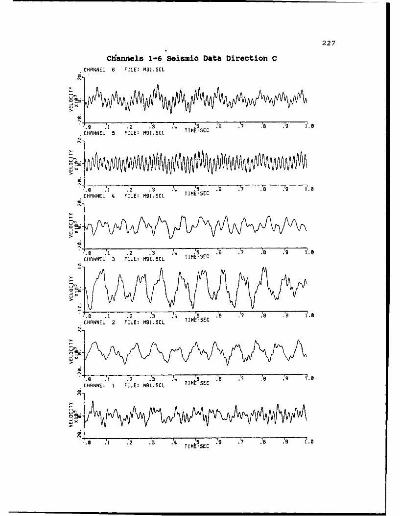
227

Channels 1-6 Seismic Data Direction CCHANNEL 6 FILE: M91.SCL

0 .'1 .'2 .'3 .14 .,5 .'6 7 .'s .,9 li. a

CHANNEL 5 FILE: Mgl.SCL TIME-SEC

G

CN

.'1 .2 .3 .q .5 .6 .7 .8 1.0CHANNEL 4 FILE: M9I.SCL TIME-SEC

L.. -.0 .'1 .'2 .'3 .4 .5 " 6 .'7 .'8 1'.,CHANNEL 3 FILE: M91.SCL TIME-SEC

o-Ujx

' .0 .1 .'2 .'3 ,' - .6 7 .'8 ..9 .

CHANNEL 1 FILE: M91.SCL TIME-SEC

lx

. . .'2 .'3 . t '5 EC 6 .7 .,8 A.9

.' .' .'3 .,q 567 .0 .

228

Cfinnels 7-12 Seismic Data Direction CCHANNEL 12 FILE: M91.SCL

.0 .'1 .2 .3 .q .5 .6 .' 9

CHANNEL 1I FILE: M9I.SCL TIMES3EC

CHANNEL 10 FILE: M91.SCL TIMESEC

-j

CHANNEL 8 FILE: M91.SCL TIME-SEC

CHANNEL 7 FILE: M91.SCL TIMESEC

TIMO-SEC

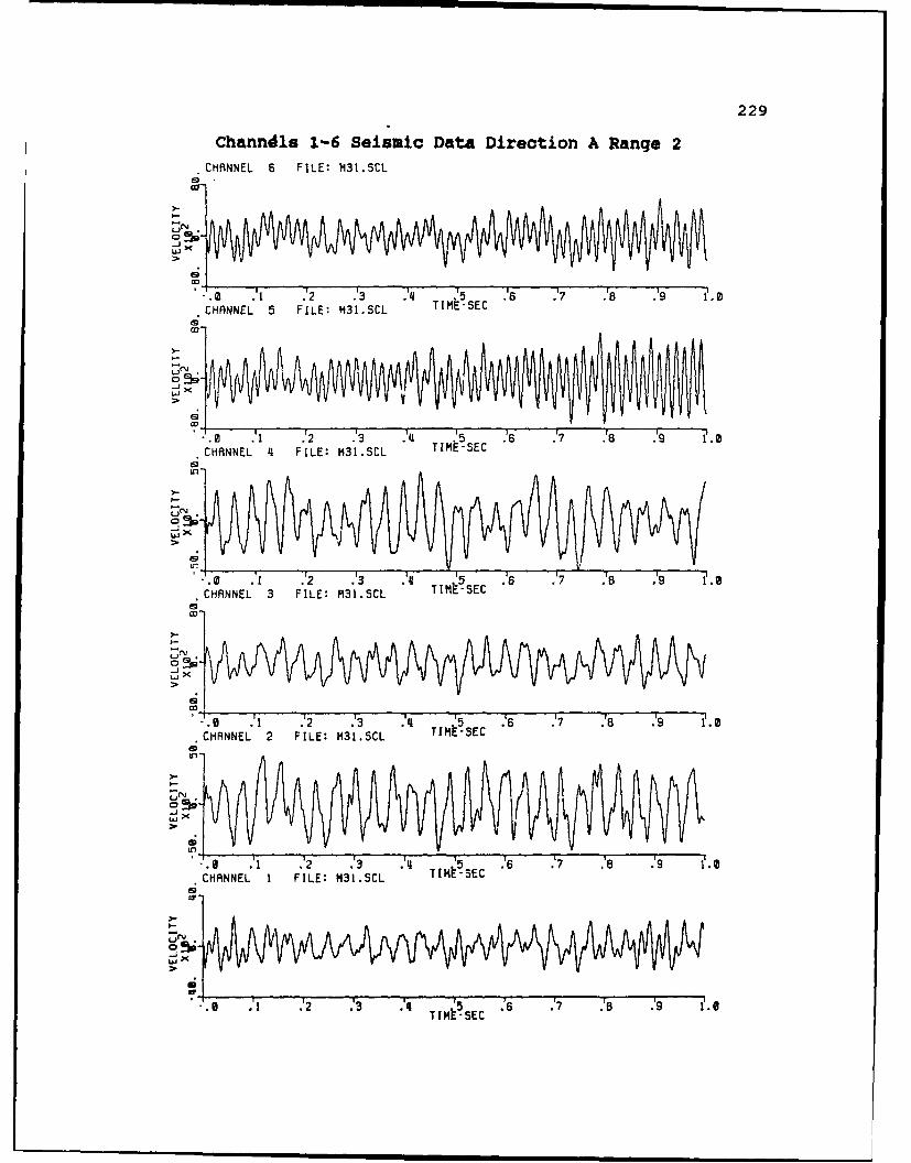
229

Channdl. 1-6 Seismic Data Direction A Range 2CHANNEL 6 FILE: M31.SCL

Lu

* . .1 .'2 .,3 A' .'5 .'s .'7 a *' ie

CHANNEL 2 FILE: M31.SCL TIME-SEC

W-

CHANNEL 1 FILE: M31.SCL TIMt-SEC

U)

.CHANEL3 FIE: 31 .SCL TI~t-SEC

230

Ch~annels 7-12 Seismic Data Direction A Range 2

CHANNEL 12 FILE: M31.SCL

In

- 1 .'2 .'3 .,q .5 : .7 .'8 A9 LCHANNEL 11 FILE: M31.SCL TIME-SEC

7 . .11 .'2 .'3 .,4 T .5 .,6 .'7 ' 'CHANNEL 90 FILE: M31.SCL TIM-SEC

CHNE FL:M1SC I E

CHANNEL 7 FILE: M31.SCL TIMt-SEC

-. 1 .'2 .3 .'4 5 .'6 .'7 .'a A9 1.CHANEL 8 FILE M31SCL TIMt-SEC

231

Channels 1-6 Seismic Data Direction B Range 2

CH ANNEL 6 FILE: M61.SCL

CHANNEL 5 FILE: M61.SCL TIME-SEC

u

-.0 .2 .'3 ,4 .5 .6 .7 .a .g 1.a

CHANNEL q FILE: M61.SCL TIME-SEC

CHANNEL 3 FILE: K61.SCL TIME-SEC

cvJ

-.0 .'1 .2 .'3 4 .5 26 .'7 .8s A' 1

CHANNEL 2 FILE: M61.SCL TIME-SEC

-J

CHANNEL I FILE: M61.SCL TIMt-SEC

Ix

.'1 .'2 .'3 .,q TIMO-5EC . '

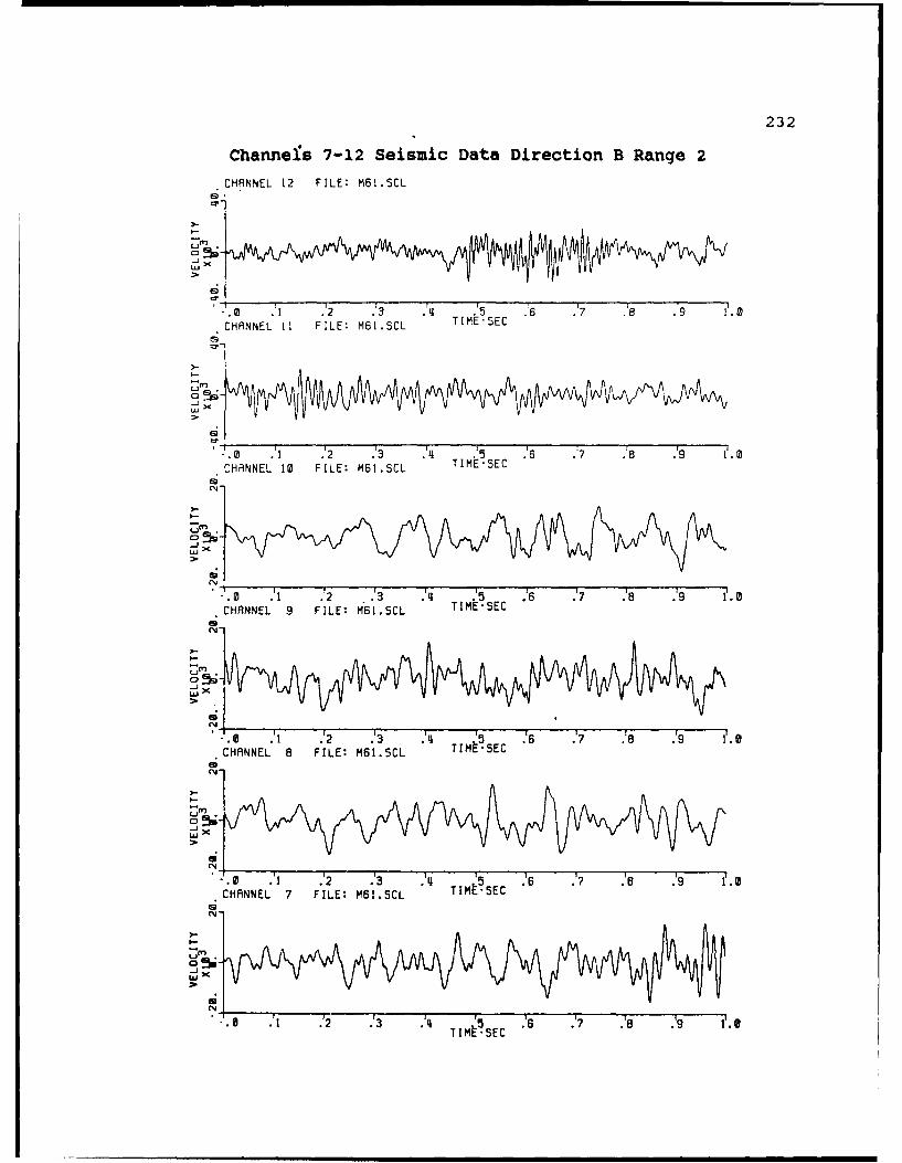
232

Channels 7-12 Seismic Data Direction B Range 2

CHANNEL 11 FILE: M61.SCL TIME-SEC

.CHANNEL 19 FILE: M61.SCL TIME-SEC

I-)

-.0 .'1 .'2 .3 .4 .'5 .6 .'7 .8s .,q .0CHANNEL 9 FILE: M61.SCL TIME-SEC

04I

CHANNEL 8 FILE: M61.SCL TmIESEC

. .'1 .'2 .'3 .A 5 .6 .'7 .'e .A f.0CHANEL 7 FILE M61SCL TIMt-SEC