Real-Time Implementation of a Near eld Broadband Acoustic Beamformer

Real -Time Implementation

of a Nearfield Broadband

Acoustic Beamformer

Eric Andre Lehmann

Dipl. El.-Ing. ETHZ

A thesis submitted for the degree of Master of

Philosophy of the Australian National University

Department of Engineering

Faculty of Engineering and Information Technology

The Australian National University

November 2000

Declaration

The contents of this work are the result of original research and have not been submitted

for a similar or higher degree to any other university or institution.

This thesis is the result of my own work and all sources used in it have been furthermore

acknowledged.

Eric Andre Lehmann

November 2000

i

Abstract

The domain of array signal processing constitutes a field of study where many interesting

and challenging projects can be undertaken. The work presented in this thesis is motivated

by the implementation of a nearfield broadband beamformer using an array of acoustic

sensors, which can be typically used for applications in speech acquisition. The objective

of this work is to practically test this beamformer, and to create a fully integrated system

that can be used to develop and implement similar designs.

Based on theoretical principles, several software simulations performed with this type of

array application have shown that it is possible to successfully implement the beamformer.

However, several problems generally arise when considering a real-hardware realization of

such a design, mainly related to the development of specific signal processing tasks. The

work presented here aims to provide efficient solutions to these various problems. It focuses

mainly on the design of the digital filters required for the beamformer, considering different

aspects related to a specific implementation using digital signal processors.

Different filter types and coefficient computation methods are considered for this imple-

mentation. The final design has to be furthermore developed in keeping with the different

limitations implied by the hardware and software tools used to perform the digital pro-

cessing of the sensor signals.

An array consisting of 15 microphones and using an FIR filtering principle is then prac-

tically realized, and different experiments are finally performed in an anechoic environment

with such a device. This thesis also presents some practical measurements obtained with

this beamformer, which shows some promising results.

ii

Acknowledgments

The year I have spent in Australia working on the Master project presented in this thesis

has been probably one of the most eventful so far in my life. Not only from an educational

point of view with the completion of this thesis, but also from a social and cultural point

of view after having lived far away from home and in such an amazing country for more

than one year.

I owe a great deal to my supervisor, Dr. Robert Williamson, who personally gave me

this opportunity to live such an exciting and unique experience, and who has showed such

a strong support for me throughout my stay.

My family, and specifically my parents, also deserve a very special thank you for having

given me their “approval” before I left them for such a long period of time. I know my

departure has been really difficult for them and hope that they realize now how important

their assent was for me.

Also, I would particularly like to thank Cressida for her kind and loving support, and

for having contributed to make my stay in Australia so enjoyable. Many thanks are also

addressed to her family for having given me literally a second home away from home.

All my friends in Switzerland, together with my new Australian acquaintances, have

also played an important role in the successful completion of my studies, through their

company and supportive friendship.

Last but not least, I would like to acknowledge gratefully all the staff members in the

Department of Engineering of the ANU who helped me in many ways during my work.

This concerns notably Bruce Mascord who made a great effort in order to finish assembling

the anechoic chamber as quickly as possible, for me to be able to use it before the due

date of my thesis.

iii

Contents

1 Introduction 1

2 Beamformer Theory Background 5

2.1 Beamformer Design Theory . . . . . . . . . . . . . . . . . . . . . . . . . . . 5

2.2 Other Beamformer Considerations . . . . . . . . . . . . . . . . . . . . . . . 9

2.2.1 Reduction of the Array Size . . . . . . . . . . . . . . . . . . . . . . . 9

2.2.2 Number of Modes to Consider . . . . . . . . . . . . . . . . . . . . . 9

2.2.3 Implications on the Operating Frequency Range . . . . . . . . . . . 10

2.2.4 Other Beamformer Improvements . . . . . . . . . . . . . . . . . . . . 11

2.3 Summary . . . . . . . . . . . . . . . . . . . . . . . . . . . . . . . . . . . . . 11

3 Hardware and Software Setup 12

3.1 Description of the SCOPE System . . . . . . . . . . . . . . . . . . . . . . . 12

3.1.1 The SCOPE System: Hardware Part . . . . . . . . . . . . . . . . . . 13

3.1.2 The SCOPE System: Software Part . . . . . . . . . . . . . . . . . . 14

3.2 Other Tools Used . . . . . . . . . . . . . . . . . . . . . . . . . . . . . . . . . 17

3.2.1 The A/D and D/A Converter . . . . . . . . . . . . . . . . . . . . . . 17

3.2.2 Other Software . . . . . . . . . . . . . . . . . . . . . . . . . . . . . . 18

3.3 Typical Experimental Setup . . . . . . . . . . . . . . . . . . . . . . . . . . . 18

4 Digital Filter Design 21

4.1 Digital Filter Types . . . . . . . . . . . . . . . . . . . . . . . . . . . . . . . 21

4.1.1 FIR vs. IIR Filters . . . . . . . . . . . . . . . . . . . . . . . . . . . . 22

4.1.2 Conclusion . . . . . . . . . . . . . . . . . . . . . . . . . . . . . . . . 24

4.2 Other General Considerations . . . . . . . . . . . . . . . . . . . . . . . . . . 24

4.2.1 Beamformer Structure . . . . . . . . . . . . . . . . . . . . . . . . . . 25

iv

4.2.2 Restrictions from the SCOPE System . . . . . . . . . . . . . . . . . 29

4.3 FIR Filter Design . . . . . . . . . . . . . . . . . . . . . . . . . . . . . . . . . 33

4.3.1 The Frequency Sampling Method . . . . . . . . . . . . . . . . . . . . 33

4.3.2 Further Developments Based on the Frequency Sampling Method . . 38

4.3.3 Conclusion . . . . . . . . . . . . . . . . . . . . . . . . . . . . . . . . 44

4.3.4 Last Filter Design Considerations . . . . . . . . . . . . . . . . . . . . 44

4.4 Processor Related Considerations . . . . . . . . . . . . . . . . . . . . . . . . 47

4.4.1 Fixed Point vs. Floating Point Representation . . . . . . . . . . . . 47

4.4.2 Finite-Wordlength Effects . . . . . . . . . . . . . . . . . . . . . . . . 48

4.4.3 Conclusion . . . . . . . . . . . . . . . . . . . . . . . . . . . . . . . . 49

4.5 Summary . . . . . . . . . . . . . . . . . . . . . . . . . . . . . . . . . . . . . 50

5 Practical Implementation and Results 51

5.1 Software Implementation . . . . . . . . . . . . . . . . . . . . . . . . . . . . . 51

5.1.1 FIR Coefficients Handling . . . . . . . . . . . . . . . . . . . . . . . . 52

5.1.2 Filter Module Structure . . . . . . . . . . . . . . . . . . . . . . . . . 53

5.1.3 General Beamformer Project . . . . . . . . . . . . . . . . . . . . . . 57

5.2 Hardware Implementation . . . . . . . . . . . . . . . . . . . . . . . . . . . . 59

5.3 Results . . . . . . . . . . . . . . . . . . . . . . . . . . . . . . . . . . . . . . . 60

5.3.1 Transfer Function Measurements . . . . . . . . . . . . . . . . . . . . 61

5.3.2 Practical Beamformer Result . . . . . . . . . . . . . . . . . . . . . . 62

5.4 Conclusion . . . . . . . . . . . . . . . . . . . . . . . . . . . . . . . . . . . . 63

6 Conclusion and Future Research 64

A Filter and Coefficient Modules under SCOPE 67

A.1 General Module Principle . . . . . . . . . . . . . . . . . . . . . . . . . . . . 67

A.2 Dynamically Updatable Filters . . . . . . . . . . . . . . . . . . . . . . . . . 69

A.2.1 The Filter Module . . . . . . . . . . . . . . . . . . . . . . . . . . . . 70

A.2.2 The Coefficient Module . . . . . . . . . . . . . . . . . . . . . . . . . 71

A.3 Summary . . . . . . . . . . . . . . . . . . . . . . . . . . . . . . . . . . . . . 72

B Beamformer Design Interface 73

B.1 Low-Pass Filter Section . . . . . . . . . . . . . . . . . . . . . . . . . . . . . 73

v

B.2 Beamformer Section . . . . . . . . . . . . . . . . . . . . . . . . . . . . . . . 76

B.3 Common General Features . . . . . . . . . . . . . . . . . . . . . . . . . . . . 79

B.4 Other Useful Matlab Function . . . . . . . . . . . . . . . . . . . . . . . . . . 80

B.5 Conclusion . . . . . . . . . . . . . . . . . . . . . . . . . . . . . . . . . . . . 81

C Signal Gain Calibration 82

C.1 Calibration Principle . . . . . . . . . . . . . . . . . . . . . . . . . . . . . . . 82

C.2 Controller Simulation with Matlab . . . . . . . . . . . . . . . . . . . . . . . 84

C.3 SCOPE Calibration Module . . . . . . . . . . . . . . . . . . . . . . . . . . . 87

C.4 Calibration Method for an Array of Microphones . . . . . . . . . . . . . . . 92

C.5 Results . . . . . . . . . . . . . . . . . . . . . . . . . . . . . . . . . . . . . . . 93

D Room Reverberation Measurements 94

D.1 Reverberation Time Measurements . . . . . . . . . . . . . . . . . . . . . . . 94

D.2 Software Developments . . . . . . . . . . . . . . . . . . . . . . . . . . . . . . 96

D.3 Octave-Band Analysis . . . . . . . . . . . . . . . . . . . . . . . . . . . . . . 99

E SCOPE “Troubleshooting” 102

E.1 SCOPE Related Problems . . . . . . . . . . . . . . . . . . . . . . . . . . . . 103

E.2 Assembler Language Hints . . . . . . . . . . . . . . . . . . . . . . . . . . . . 105

F CD Contents 107

F.1 Matlab Files . . . . . . . . . . . . . . . . . . . . . . . . . . . . . . . . . . . . 107

F.2 SCOPE Files . . . . . . . . . . . . . . . . . . . . . . . . . . . . . . . . . . . 108

F.3 Miscellaneous Folders . . . . . . . . . . . . . . . . . . . . . . . . . . . . . . 110

Bibliography 111

vi

Glossary of Definitions and

Abbreviations

Several specific terms are used in this thesis in conjunction with some special hardware

and software components, or related to the general theory of digital signal processing.

These different definitions and abbreviations are listed and briefly explained below.

A16 16 channel A/D and D/A converter from CreamWare

A/D Analog to Digital

AX-490 Power audio amplifier from Yamaha

BPF Band-Pass Filter

D/A Digital to Analog

DFT Discrete Fourier Transform

DSP Digital Signal Processing or Digital Signal Processor

ESIB Elementary Shape Invariant Beamformer

FFT Fast Fourier Transform

FIR Finite Impulse Response

Flops Floating Operations

IDFT Inverse Discrete Fourier Transform

IIR Infinite Impulse Response

I/O Input – Output

LPF Low-Pass Filter

M80 8 channel microphone pre-amplifier and power amplifier from PreSonus

MLA7 8 channel microphone pre-amplifier from Yamaha

PID Proportional – Integral – Derivative

vii

SNR Signal to Noise Ratio

Windows Computer operating system

The work presented in this thesis also makes use of the SCOPE system, a powerful

development platform for DSP-based applications. Throughout the thesis, this special

device will be always referred to with capital letters in order to differentiate it from the

common English word. The list below presents different specific terms used in conjunction

with this application and its use. More details can be found in [15] and [14] if needed.

Project Audio or DSP design developed in software with SCOPE

Module Basic building block in a project

Surface Graphical user interface of a module

DSP Dev. DSP Developer’s Kit: a second version of the SCOPE application allow-

ing the programming of custom modules

viii

Chapter 1

Introduction

The field of array signal processing has been subject to a great deal of engineering and

technical research over the past few decades (see e.g. [8, 9, 10, 20, 1]). This topic is still

being intensively studied, and new theories are constantly being published and tested

in several laboratories around the world. However, although most of these theoretical

considerations attempt to solve problems related to real-world applications and are clearly

motivated by practical implementations, many of them only report results obtained from

pure software simulations. Very few of them have actually considered the various problems

and restrictions involved in a real hardware implementation of the proposed acoustic array

principles.

There exist many different application areas where an array of microphones could be

efficiently implemented as a replacement of the technology currently in use. As a typical

example, let’s consider the problem of speech signal acquisition. In many cases, it is neither

practical nor desirable to have a microphone very close to the talker’s mouth (such as e.g.

for hands-free phones [2], teleconferencing systems [3, 4], auditoria sound systems [5], etc.),

implying the acquisition of a rather reverberant signal in many environments. A general

approach to acquiring a “cleaner” signal is to use an array of microphones [2]. This is

directly analogous to a phased-array radio antenna [6], but there are several features of

the microphone array problem that distinguish it from classical radio phased-arrays. The

relative bandwidths are much larger and the operating frequencies much lower than for

radio arrays. These differences both require and allow more sophisticated digital signal

processing techniques to be used.

The implementation of a general broadband beamformer typically designed for speech

CHAPTER 1. INTRODUCTION 2

processing is presented in this work, which focuses principally on the various DSP factors

to take into account when developing and testing such a design on real hardware. This

beamformer has been developed mainly according to the theory presented in the journal

article Nearfield Broadband Array Design Using a Radially Invariant Modal Expansion, by

T. Abhayapala, R. Kennedy and R. Williamson [1]. This paper presents a new method of

designing a beamformer with a desired broadband beampattern and focusing capability in

order to operate at virtually any radial distance from the sound source. A typical example

of a microphone array used for speech acquisition is also given in this article and will be

used as a reference model throughout the thesis.

The practical results obtained with the array will also be presented at the end of the

thesis. However, it should be specially noted at this point that the main purpose of this

work is not a detailed and deep investigation of the array efficiency, and no specific analysis

will be performed for a possible improvement of the beamformer. Instead, this thesis will

consider the more subjective aspects of the array, and will answer questions like: “Consid-

ering the targeted application, does the beamformer generate a result that sounds good?”.

Chapter 2 briefly describes the different theoretical aspects of the beamformer imple-

mentation as they are presented in [1]. This chapter only contains the basic beamforming

theory needed to understand the developments made in this thesis, and the reader is

referred to [1] for more specific information if required.

Processing the signals from a microphone array, which can be made up of a sub-

stantial number of sensors, usually requires a significant computing power. A high-end

and professional development system for DSP-based audio applications, the SCOPE from

CreamWare, has been used to implement the different signal processing tasks needed for

this work. This relatively novel device requires some specific knowledge to operate cor-

rectly, and also implies some restrictions on the design implemented. These different issues

are described in detail in Chapter 3.

The beamformer is implemented using a relatively simple structure: an array of acoustic

sensors fed into digital filters and then combined additively. Several filtering methods can

be used to process the signals from the sensors. The different issues concerning the design

of these filters are carefully considered in Chapter 4.

Chapter 5 then deals with the practical realization of the beamformer on the basis of


the previous considerations. It also presents the results obtained during the test phase of

the microphone array.

Finally, some general and concluding comments concerning possible future research on

this topic are given in Chapter 6, based on the work presented in this thesis.

This thesis also contains a consistent appendix section describing in detail various

principles and implementations that have been used for the practical development of the

beamformer. It also presents a full description of the most important programs and files

created to this purpose. The theory of microphone arrays, and more generally the field of

digital signal processing, constitutes an important part of the research and development

work in the Department of Engineering of the ANU. Therefore, it is likely that many

students and academics are going to make use of the SCOPE system in the future. Due to

the relative novelty of this product and the very specific way it is used, it was important

to thoroughly document the different program codes and modules developed for this work

in order to make them fully understandable for other researchers in this domain.

Appendix A presents two special filter modules created under SCOPE and used in

conjunction with the beamformer implementation using an array of acoustic sensors. A

detailed description of their respective functionality and parameters is also given in order

to easily integrate them into other DSP applications developed with the SCOPE system.

Appendix B describes a graphical user interface that can be used to interactively

simulate different types of beamformer design according to the theory presented in [1].

This development tool has been programmed as a specific function under Matlab, and it

also allows the user to download new beamformer characteristics into a SCOPE project,

where the resulting beamformer signal can be generated and “acoustically assessed” in

real-time.

An important task to accomplish before undertaking the practical test of the beam-

former with an array of microphones is to accurately calibrate the different signal paths.

Appendix C describes in detail the method used to achieve this task and the corresponding

SCOPE module implementing it.

The reverberation time of a room constitutes an important acoustic parameter and has

been practically estimated in the different environments used for the experimental test of

the array. Appendix D presents the method that has been used for these measurements


together with the different practical results obtained with it.

Appendix E aims to provide some useful information concerning several common errors

that can occur during the creation of custom modules for the SCOPE DSP Dev. applica-

tion. Since a relatively time-consuming process is generally needed in order to track down

the problem causing a SCOPE module not to function properly, this appendix has been

included as a help for developers not having worked with the SCOPE system before.

A data CD has been included as well in this thesis. It contains the most important

files created and mentioned in this work for further possible developments based on them.

Appendix F gives a content listing of this CD and also describes briefly each file, un-

less a specific section of the thesis is devoted to them. In this case, a reference to this

corresponding section is provided instead.

Chapter 2

Beamformer Theory Background

This chapter aims to provide enough beamforming theory background for the reader to

completely understand the theoretical developments of the coming chapters.

The basic principles and equations of the beamformer design given in [1] are reproduced

and explained in the first part of this chapter. It also highlights the most important points

to consider in view of a practical DSP implementation of the beamformer described in this

paper. If more information on this topic is required, the interested reader is referred to [1]

for the complete theoretical developments.

The second section discusses some design modifications necessary to yield a more

relevant beamformer, notably from the point of view of a practical approach using the

hardware and software tools at disposal.

2.1 Beamformer Design Theory

The problem of designing a uniformly spaced array of sensors for farfield operation at a

single frequency (or within a narrow band of frequencies) is well understood from general

array theory [18, 19]. However when it is desired to receive signals over a wide band of

frequencies the problem of broad banding a sensor array arises. Works like [20, 21] deal

with this problem and give different ways to solve it.

Most of the array processing literature assumes a farfield source having only plane

waves impinging on the sensor array. However, in many practical situations, such as mi-

crophone arrays in car environments [7], the source is well within the nearfield. The use

of farfield assumptions to design the beamformer in these situations may severely degrade

the beampattern.

CHAPTER 2. BEAMFORMER THEORY BACKGROUND 6

The theory given in [1] presents a new method of designing a beamformer having a

desired broadband beampattern as well as a focusing capability to operate at any radial

distance from the array origin. It is based on writing the solution to the wave equation

in terms of spherical harmonics and allowing a nearfield beampattern specification to be

transformed to the farfield. The nearfield beamformer is then designed with the subsequent

use of well understood farfield theory [22].

An important result of the beamforming theory developed in [1] is that it describes a

systematic way of designing nearfield broadband sensor arrays by decomposing the beam-

former into three levels of filtering as follows:

1. A beampattern independent filtering block consisting of elementary beamformers.

2. Beampattern shape dependent filters.

3. Radial focusing filters, where a single parameter can be adjusted to focus the array

to a desired radial distance.

According to this principle, the basic block diagram of a general one-dimensional broad-

band beamformer can be easily built as depicted in Figure 2.1. Table 2.1 gives the corre-

sponding definitions for the symbols and variables used in this figure.

k Wave number: k = 2πf/c

zi Position of i-th sensor

r Focusing distance from array origin

Si i-th sensor

gi Spatial weighting term

Fn(zi, k) Elementary filter of mode n

αn(k) Beam shape filter of mode n

Gn(r, k) Radial focusing filter of mode n

ESIBn Elementary Shape Invariant Beamformer of mode n

Table 2.1: Beamformer definitions.

As in [1], the parameter k will be simply referred to as frequency in this thesis. The

equations for the computation of the different filters given in the lowest part of Table 2.1


0 g

L g -

L g

) , ( 0 k z F L -

) , ( 0 0 k z F

) , ( 0 k z F L

) , ( 0 k r G +

+ +

0 ESIB

) , ( k z F L N -

) , ( 0 k z F N

) , ( k z F L N

+

+ +

N ESIB

+

+

L S -

0 S

L S

0 .

) , ( k r G N N .

) ( k

) ( k

Figure 2.1: Block diagram of a general one-dimensional broadband beamformer.

are defined in [1] and reprinted here for convenience.

Fn(zi, k) = (−j)nJn+ 1

2(kzi)

√kzi

, (2.1)

Gn(r, k) αn(k) = βn(−j)n+1

π

√

k

r

ej(k−k0)

H(1)

n+ 12

(kr), (2.2)

where:

Jn+ 12(·) is the half odd integer order Bessel function,

βn is a mode dependent constant,

k0 is an arbitrarily chosen nominal frequency in the considered beamformer frequency

range,

H(1)

n+ 12

(·) is the half odd integer order Hankel function of the first kind.


When considering the design of a specific broadband beamformer, the following equa-

tions can be used to determine the minimum number L of sensors needed per one array

side, as well as the number Q of uniformly spaced sensors in one side of the array:

Q =

⌈aN (1 + γ)

π

⌉

, (2.3)

L = Q +

log(

aN (1+γ)Qπ

ku

kl

)

log(

1 + πaN

)

, (2.4)

where:

γ is an additional parameter introduced to reduce the effect of spatial aliasing in case of

a nearfield beamformer design,

aN corresponds to the upper cut-off frequency of the elementary filter of the highest

considered mode N ,

ku, kl are respectively the upper and lower limits of the considered beamformer frequency

range.

Further information (concerning e.g. the spacing of the sensors, the computation of

the weighting terms gi, the values of the different constants mentioned above, etc.) can be

found in [1] if required.

To conclude and validate this new theory, the example of a one-dimensional broadband

beamforming design using the techniques described above is given at the end of [1]. This

array implementation is suitable for speech acquisition with a beampattern that is invariant

over an operating frequency range of 1:10 (set in [1] from 300 to 3000 Hz). The maximum

mode index N is limited to a value of 15 for this practical design, and the beamformer is

developed from a constant Chebyshev beampattern with an attenuation of 25 dB outside

the main lobe.

From these parameter settings and according to the different equations given above

and in [1], the resulting microphone array needs a total number of 41 sensors and an overall

length of approximately 5 meters in order to completely match the desired specifications.


2.2 Other Beamformer Considerations

The developments made in [1] and given in the previous section have been verified from

a purely theoretical point of view. According to the example design described in the last

section of the paper, the results obtained from a software simulation show that a satisfac-

tory beamforming ability can be achieved with an implementation of this array. However,

the work presented in this thesis focuses on the practical aspects of the beamformer re-

alization, and some of the assumptions made in [1] need to be modified or re-defined in

order to yield more realistic and relevant specifications.

2.2.1 Reduction of the Array Size

The size and complexity of an array of microphones mainly depend on the targeted “real-

life” application. For example, the length of an array developed for auditoria systems will

be obviously different from one used for hands-free phones in car environments, where

smaller distances have to be taken into account.

Independently of the targeted application and for obvious practical reasons, it is how-

ever technically neither optimal nor desirable to implement and test a beamformer design

the size of that described in [1]. The testing methods and environments used for this work

do not allow the implementation of such a large design. Besides, the total number of sen-

sors at disposal for the testing phase was limited to 15 at the time of the submission of

this thesis. It is then clear that this considerable reduction of the number of sensors will

not allow an array implementation with beamforming capability as it is ideally described

in [1]. The consequences of this restriction implied on the beamformer performance will

be considered later in this section.

2.2.2 Number of Modes to Consider

Another question arises concerning the total number of modes to consider for the imple-

mentation. The theory described in [1] is based on the fact that every arbitrary beampat-

tern br(θ, φ; k) can be formed by appropriately choosing the frequency-dependent param-

eters αn(k) in the following expression:

br(θ, φ; k) =∞∑

n=0

αn(k) · ESIBn ,


where ESIBn corresponds to the Elementary Shape Invariant Beampattern of n-th mode,

which is independent of the current beamformer design.

Limiting this sum to the first N + 1 termsa reduces the number of practically real-

izable beampatterns. It is hence desirable to maximize the index N of the highest mode

considered when designing a beamformer according to this theory. However, it is stated in

[1] that for most practical beampatterns, the characteristic coefficients αn(k) are typically

zero for n > 15, and hence higher order filters need not be considered. As a consequence

of these observations, the design implemented in this work has made use of a maximum

number of 16 modes (that is N = 15).

2.2.3 Implications on the Operating Frequency Range

An important consequence of maximizing the index N of the highest mode considered

for the design is a corresponding increase of the variable aN used in the computation of

the minimum number of sensors needed in the array. In fact, it can be quickly seen that

Equation 2.3 cannot be satisfied with the current parameter settings chosen: a value of

7 is obtained for Q,b requiring more than 15 sensors in the array, which is already in

contradiction with the number of microphones at hand. This is despite the fact that the

numerical value for the constant aN is not uniquely defined for the elementary filters, and

that another cut-off frequency than the one given in [1] can also be chosen.

Likewise, Equation 2.4 defining the total number of microphones cannot be satisfied

either, and as the only free parameter in this equation, it is impossible to match the desired

operating frequency range ku/kl. However, the array is still developed for a general appli-

cation in speech acquisition and has to be operated over a frequency range of 1:10 or so.

As it will be seen later on, the result will be a beamformer that is not frequency-invariant

anymore, but that shows a degradation of its beampattern for certain frequencies. The

width of the main beam will also be larger than theoretically expected. The exact impli-

cation on the beamformer performance is difficult to predict, and it will be only during

the practical and subjective tests of the array that it can be decided whether it offers

satisfactory beamforming results despite this deterioration.

As a result of these considerations, the array that will be practically implemented in

aThat is summing the terms from n = 0 to n = N .bWith the worst case setting γ = 0.


this work will consist of 15 equally spaced microphones.

2.2.4 Other Beamformer Improvements

Several other parameters can be adjusted in the array design described in [1], and different

tests and simulations with these variables have been accomplished in an attempt to opti-

mize the beamformer performance under the practical restrictions of all kind mentioned

previously.

However, the influence of these parameter and design changes on the beamformer qual-

ity have shown to be rather insignificant, and none of the tested parameters has proved to

have as much impact on a possible design improvement as the variable representing the

number of sensors (L). Increasing the value of this latter would obviously be the only way

to radically improve the beamforming ability of the array.

A specific design tool (BDIgui.m, standing for Beamformer Design Interface) has been

implemented with Matlab in the frame of this work to offer a considerable help in the

development of beamformers based on the theory presented in [1]. This interface allows the

user to freely “play” with the different beamformer design parameters, and to dynamically

see the different variations resulting in the beampattern over the desired frequency range.

This program can also be used to compute the different filters required to implement the

array. More information on this development tool can be found in Appendix B.

2.3 Summary

The background beamformer theory has been presented in this chapter. First, the main

design equations and principles as given in [1] have been described in conjunction with the

beamformer implemented in this work, followed by slight changes in the design proposed

according to more relevant practical considerations.

The remainder of this thesis, and especially Chapter 4 which specifically deals with

the design of the different filter blocks of the beamformer implementation, will constantly

refer to the theory presented in this section of the thesis.

Chapter 3

Hardware and Software Setup

Since the different beamforming filters will be ultimately implemented on real hardware, it

is important to be aware of the various constraints this implies on the beamformer design

described in Chapter 2. This section of the thesis briefly describes the general working

principles of the most important hardware and software tools used in this work. It is not

meant to provide full and thorough details about these tools. If needed, more specific

technical data can be accessed through different sources like operating manuals, online

documentation, etc.

This chapter is organized as follows. A description of the main tool used in this work

(the SCOPE system) is given in the first section, followed by a quick listing of several

other devices of lesser importance. Finally, a general overview of a typical experimental

setup is depicted in the last section of this chapter.

After having read this part of the thesis, the reader should be aware of the most

important factors to consider concerning the hardware and software setup used in this

work, and hence have the necessary knowledge for a full understanding of the further

developments made in this thesis.

3.1 Description of the SCOPE System

In order to implement digital signal processing tasks, the use of a DSP-based system over

other dedicated-hardware solutionsa is motivated by several reasons, the most important

of which being probably the high degree of flexibility of DSP programming [31, 35, 36].

aRanging from programmable logic devices to full custom designs like standard cells and gate arrayASICs.

CHAPTER 3. HARDWARE AND SOFTWARE SETUP 13

The short implementation and test times, as well as the low development costs are also

valuable advantages in favor of such DSP-based solutions.

The work presented in this thesis has made an intensive use of a professional device

recently introduced on the market of the high-end development systems for DSP-based

audio applications: the SCOPE system, developed by the German company CreamWare

Datentechnik GmbH. This product roughly consists of a DSP board with audio and PCI

bus interfaces, driven by an intuitive and dynamic software interface. These two major

parts are described below.

3.1.1 The SCOPE System: Hardware Part

The hardware part of the SCOPE system consists of a computer PCI board containing

fifteen of one of the fastest general-purpose floating-point DSPs currently available: the

32-bit ADSP-2106x SHARC DSP from Analog Devices. Figure 3.1 shows a picture of the

SCOPE board.

Figure 3.1: The SCOPE board.

A SHARC DSP allows a maximum of three floating-point operations per clock cycle

at a working frequency of 60 MHz. Hence, the SCOPE board is capable of delivering

a peak performance of 2.7 GFlops/s. As it will be seen later on, this device provides

enough computing power to process the audio signals from a medium-sized microphone

array sampled with a relatively high frequency. If more processing power happens to be


necessary, the SCOPE system also allows up to five such boards to be easily cascaded via

an additional external bus interface.

For the communication of audio signals with other external devices, the SCOPE board

has at its disposal a total of 24 digital I/O channels, implemented with three ADAT-

compatible optical interfaces.

Details concerning the specific architecture of the ADSP-2106x DSP chip (computation

units, memory organization, registers, etc.) and its programming (instruction set reference,

numeric formats, etc.) can be accessed in the product documentation provided by Analog

Devices (see e.g. [11, 12, 13]).

3.1.2 The SCOPE System: Software Part

To complete the SCOPE system, the DSP board is driven by a modular graphical user

interface [14] installed on a computer running a Windows operating system. Figure 3.2

gives an overall view of a typical SCOPE user interface. It is subdivided into several dif-

Figure 3.2: Typical user interface of the SCOPE system.

ferent areas, including the project window (largest window in Figure 3.2), which contains

the different modules currently downloaded and running in the DSPs. These modules can

be dynamically “dragged and dropped” into the current project (from the file browser


window nearby) and connected to each other as desired in order to construct arbitrarily

complex audio DSP applications.

An audio signal connected to one of the 24 digital input channels of the SCOPE board

can be easily accessed within the SCOPE project through one of the Scope ADAT source

modules. In the same way, audio signals inside the project can be made available on one of

the 24 output channels by means of one of the three Scope ADAT destination modules.

Likewise, the internal audio signals inside the SCOPE project can also be accessed by

any other application running under Windows (like e.g. Matlab, or any other digital audio

authoring software) for further processing and analysis by simply connecting the desired

signals to a specific pre-existing module in the project.

The sampling frequency of the SCOPE project can be set to different values, depending

on the status currently defined for the system (clock master or slave). In master mode,

the working frequency can be set from within SCOPE to either 32, 44.1, 48 or 96 kHz.

When the SCOPE board is operated as a clock slave, it accepts an external wordclock

signal ranging from 30 to 100 kHz.

This sample rate is globally defined for the whole SCOPE project. It is identical for

all the modules and audio signals comprised in it, as well as all the input and output

signals from or to external devices or Windows applications. As it will be seen later on in

this work, this fact implies a substantial restriction for the development of special signal

processing implementations, such as for instance multirate filters.

More information about this basic version of the SCOPE application software can be

found in the product documentation of the SCOPE system [14].

Custom Module Creation

The basic SCOPE software is delivered with a certain number of pre-existing modules,

many of which are specifically targeted for recording studio or music authoring applications

(the selection includes modules for high-quality mixing, effects processing and synthesis,

as well as a number of different MIDI controllers). Whereas these modules are of great

interest for the professional audio industry, they fail to be really helpful for the developer


of differently oriented digital signal processing tasks.

Another version of the software, the so-called SCOPE DSP Developer’s Kit [15], has

been used on top of the basic SCOPE installation to provide the programmer with a

method of creating custom modules for more specific signal processing implementations.

With the help of this application, the creation of custom modules comes down to the direct

programming at a low level of the custom routines executed by the DSPs. The process that

has to be followed for the creation of new modules can then be divided into the following

three simple steps:

1. Development of the different program routines that will be executed by the DSPs

and implementing the desired signal processing tasks, using the Analog Devices

ADSP-21000 Assembler language [11].

2. Pre-processing of the written program code (including code compilation and encryp-

tion) using executable files provided by Analog Devices and CreamWare.

3. Making the resulting compiled files available for the SCOPE software (by placing

them into the correct directory) and simply loading them as new modules into a

project.

The programming of the DSP code (first step in the list above) has to be carefully

developed in accordance with strict restrictions implied by the SCOPE system, notably

concerning the usage of the different DSP registers, the number of available DSP clock

cycles, or the different ways to access the module inputs and outputs (see [15]).

The SCOPE software also allows the developer to design a graphical interface for the

newly created module, which provides user-friendly access to the module settings and ad-

justable parameters.

A further relatively important feature of this second SCOPE version is the ability to

update the Assembler code of a module from within the SCOPE project by means of the

Reload DSP File command. This option allows a new program code to be downloaded

into an existing and running module in the project without the need to restart the whole

application. Even though no structural changes are allowed with this method (like e.g.

adding or removing module inputs or outputs), it still provides the programmer with a


quick way to make progressive changes to the code of a module under development, and

also to implement some more specific functions taking advantage of this feature.

The process described here allows an easy and quick development of relatively complex

digital signal processing implementations, the only implication for the developer of new

modules being a careful programming of the Assembler code realizing the desired tasks.

More information on the different subjects described here in relation with the SCOPE

system can be found in [15] if required.

Parallel Processing

One of the most important features of the SCOPE system is its ability to execute the

developed DSP applications on several or all of the fifteen DSPs in parallel. This multi-

processing is completely controlled by the SCOPE software that decides itself which DSPs

are going to be loaded with the different routines to execute. However, this decision is made

on a relatively simple basis by the SCOPE operating system, which simply downloads a

module code into one of the DSPs after having checked that enough memory and processing

power are available in it. The SCOPE is furthermore unable to subdivide the program code

of a module into several smaller routines that would be distributed evenly over the fifteen

DSPs.

These facts are relatively important to note because they imply that it is impossible

to create a module which would require more memory or processing power than it can be

provided by one single DSP.

3.2 Other Tools Used

Several other devices have been used for the developments and tests described in this work,

including different types of microphones and microphone pre-amplifiers. In this section, it

is most important to provide the reader with some information concerning the A/D and

D/A converters that have been used for these practical experiments.

3.2.1 The A/D and D/A Converter

This work has made use of the A16 developed by CreamWare, which is a compact multi-

channel A/D and D/A converter. It is capable of converting simultaneously a total of

sixteen analog audio channels to digital and sixteen digital audio channels to analog.


The multi-channel digital connections are implemented using two ADAT-compatible I/O

interfaces. This allows a direct audio data communication through optical fibers with the

SCOPE board.

Even though the operating manual describes the A16 as an 18-bit converter, a quick

look at the other technical data shows that this device cannot completely meet this per-

formance. The typical THD+N for the A/D conversion is 0.003%, corresponding to a

dynamic range of approximately 90 dB. According to the basic rule of a dynamic range

increase of 6 dB per bit, this in turn corresponds to approximately fifteen bits. Conse-

quently, only the first fifteen bits of the audio samples provided by the A16 are relevant.

As a result, the audio data appears in the SCOPE project as 16-bit signed fractional values

(two’s-complement representation).

The A16 can also be defined by the user as a wordclock master or slave. As a master

device, the sampling frequency of the A16 can be set to either 44.1 or 48 kHz, and it

accepts a minimum and maximum frequency of 38 and 50 kHz respectively when operated

as slave. With the description of the SCOPE system given previously in Section 3.1.2, it

can be deduced then that the minimal clock frequency that can be set up for the SCOPE

board connected to the A16 is 44.1 kHz. This fact will have some implications on the

developments made later in this thesis.

3.2.2 Other Software

Several other software applications have been used in conjunction with the different devices

mentioned above. These include mainly a couple of digital audio authoring programs,

Cakewalk Pro Audio and Cool Edit Pro, used for signal recording and analysis purposes.

More information concerning their respective characteristics and functionality can be found

in the manuals provided with these products (see [16] and [17]). The mathematical package

Matlab 5.3 has been also intensively used for simulation purposes throughout this work.

3.3 Typical Experimental Setup

A brief technical description of the various devices and applications used for the array im-

plementation has been given in this chapter. It has also reviewed the different implications

and restrictions they might have on the beamformer design that will be presented in the


coming sections of the thesis.

For the reader to gain an even better understanding of the different interactions of

these tools with each other, the block diagram of a typical hardware and software setup

is presented in Figure 3.3 on the basis of the descriptions given previously. This figure

depicts the different parts of the system and their interactions with each other. The plain

arrows represent streams of audio data, either analog or digital. The dashed white arrows

symbolize how this data is made available from one component to the other through

system-specific communications. The different modules and blocks enclosed in the area

labeled SCOPE Software Application define the general project currently running under

SCOPE.


(Mat

lab,

Cak

ewal

k Pr

o A

udio

, Coo

l E

dit P

ro, e

tc...

)

Mic

roph

one

Prea

mp.

(M

80, M

LA

7, e

tc...

)

A/D

- D

/A C

onve

rter

(A

16)

Pow

er A

mpl

ifie

r (M

80, A

X49

0, e

tc...

)

Ana

log

In

Ana

log

Out

ADAT Digital I/O

Cus

tom

DSP

A

pplic

atio

n D

efin

ed in

a

SCO

PE P

roje

ct

Oth

er W

indo

ws9

8 So

ftw

are

SCO

PE

Sof

twar

e A

pplic

atio

n

Opt

ical

I/O

Win

98 C

ompu

ter:

Pen

tium

III

500

MH

z, 5

12M

B R

AM

, 19

GB

Har

d D

isk

24 24

AD

AT

Des

t. M

odul

e

AD

AT

Sou

rce

Mod

ule

Wav

e D

estin

atio

n M

odul

e

Wav

e So

urce

Mod

ule

SCO

PE

Boa

rd

Figure 3.3: Typical setup used for the practical beamformer experiments.

Chapter 4

Digital Filter Design

This chapter deals with the practical realization of the filters needed for the beamformer

described in Chapter 2. A first section discusses different types of digital filters that can

be used to this purpose, and gives the motivations concerning the filter type chosen in

this work. The second section is concerned with the details of the filter implementation

in conjunction with the SCOPE system and the beamformer design theory described in

Chapter 2. Finally, the last section presents and compares different ways of computing the

desired filter coefficients. It also considers various problems that can be encountered during

the implementation of a digital filter on real DSP hardware, and presents the solutions

adopted here to efficiently deal with them.

4.1 Digital Filter Types

The first step in the design process of a digital filter is to determine the desired response

H(ω) = |H(ω)| · ej arg[H(ω)] it should present in the frequency domain. Having determined

this so-called transfer function, the designer is then confronted by the problem of imple-

menting it in software or hardware, and notably has to make a decision concerning the

type of digital filter that is going to be used.

There are three basic classes of digital filters [26]: fast transform filters (FFT scalar fil-

ters, fast transform vector or scalar filters, etc.), recursive and non-recursive filters. Other

digital principles include sub-band and block filtering. Most of the existing literature on

this topic (see e.g. [27, 28, 29, 30]) remains mainly focused on two types of digital fil-

ter realization: finite impulse response (FIR, non-recursive) and infinite impulse response

(IIR, recursive) filters. These two realization principles will also be the main objects of

CHAPTER 4. DIGITAL FILTER DESIGN 22

consideration in this section, precisely because the theory for the development and imple-

mentation of such filters has been extensively studied already and is now fully understood.

FIR and IIR filters are also the most common filter types encountered in real-life digital

applications.

4.1.1 FIR vs. IIR Filters

The general Z-transform of any causal (and consequently implementable in real-time)

digital filter with a rational transfer function H(z) can be given as:

H(z) =Y (z)

X(z)=

∑M−1m=0 amz−m

∑N−1n=0 bnz−n

, (4.1)

where:

z is the complex variable of the Z-transform,

Y (z) is the Z-transform of the filter output signal,

X(z) is the Z-transform of the filter input signal.

The realization of non-recursive FIR filters contains only feed-forward paths and rep-

resents a special case of Equation 4.1 in which all bn coefficients are zero, except for b0

which is equal to 1. In other words, the filter output is a sum of linearly weighted present

and previous samples of the input signal. In recursive IIR filter structures, some of the bn

coefficients are non-zero for n > 2, implying the existence of feed-forward as well as feed-

back paths. The output signal of IIR filters depends both on the input and the previous

output samples.

The choice of one of these two types of digital filter implementation is an important

question in the design of DSP-based applications. In the literature, the works presenting

the theory of these two filter types usually also discuss which one is more appropriate to

use. Both IIR and FIR realizations have a number of specific advantages and drawbacks

that must be carefully considered in conjunction with the targeted application rather than

from a general point of view. A relatively exhaustive listing of the different properties of

FIR and IIR filters compared to each other is given in [26].

IIR filters have several undeniable advantages and desired properties. The most impor-

tant of them is probably the ability to implement transfer functions having sharp cut-off


or high selectivity with only a small number of coefficients, thus allowing small storage

requirements, short delays, and a small number of arithmetic computations. FIR filters

usually present a low selectivity, unless high order filters are implemented. It takes on

average 5 to 10 times more coefficients (and hence more computations) for an FIR design

to achieve the same level of performance as a low order IIR filter [26].

Despite this apparent lower efficiency, FIR filters offer the important property of being

stable under any circumstances. The development process for IIR filtering on the contrary

has to carefully consider instability problems, which makes it consequently more compli-

cated. FIR filter design methods hence offer the further advantage of being usually easy

and well-defined. Another advantage of FIR filters is that they allow the implementation of

transfer functions presenting a linear phase characteristic, which is particularly important

for the beamformer considered in this work. The implementation of a filter with constant

group delay using IIR filtering would imply the development of a first filter block to ap-

proximate the desired amplitude response, followed by an all-pass correcting the phase

according to the desired specifications.

Required Filter Order

Contrary to the IIR filter development, where an exact order requirement can be evaluated

for certain filter types, the FIR order needed to obtain a given specification can only be

approximated [31]. Different such approximation methods can be found in the literature:

[32] and [33] present a series of equations for a relatively simple approximation, whereas

a more computationally complex form is given in [34]. These equations are rather compli-

cated however, and they are often only valid for pre-defined filter specifications (low-pass,

band-pass, band-stop, etc.).

The method chosen in this work to determine the number of coefficients required for an

FIR filter is based on a more subjective principle: the order of the filter is simply increased

until a satisfactory response is achieved. Two main criteria can be used in order to decide

when to stop this iterative process. First, the resulting frequency response can be analyzed

in order to determine whether it constitutes a good approximation of the desired transfer

function. A second possibility is to consider the filter behaviour in the time domain and

see if an important part of its impulse response is truncated, in which case the filter order

has to be increased more.


By using this method to determine the length of a filter, it is relatively difficult at this

stage to make sure that it is practically possible to implement the beamformer with FIR

filters. As it will be seen in a later chapter however, the SCOPE system can easily provide

the processing power and memory space required to implement accurate FIR filters for

the beamformer realization.

Longer delays of the input signals in the processing path do not constitute an issue

for the quality of the acoustic array either. These are quite small for the design presented

in this thesis anyway (in the order of size of a few milliseconds), and at this stage of

the development it is neither necessary nor important to try to reduce them. For a later

implementation where these delays may become undesirable, a different filtering method

can be used instead.

4.1.2 Conclusion

From the different considerations presented previously in this section, an implementation

of the acoustic array using FIR filtering has been chosen. This decision was also motivated

by simplicity reasons concerning a first beamformer design using the recently introduced

SCOPE system. Some more knowledge needed to be gained concerning the exact way to

operate this tool. Therefore, a simpler and more stable filter structure has been preferred

in order to avoid any further complication during the implementation of the array design.

4.2 Other General Considerations

The general Z-transform resulting from Equation 4.1 for an M -th order FIR filter is now

simply given as:

H(z) =Y (z)

X(z)=

M−1∑

m=0

hmz−m . (4.2)

The exact computation of the transfer function H(z) is determined by the different

equations given in Chapter 2 and in [1]. But before dealing with the problem of how

to compute the coefficients, some other design considerations concerning the filter struc-

ture and its transfer function must be studied. These will be considered in the following

subsections.


4.2.1 Beamformer Structure

Having opted for FIR filters, the next problem to solve is the choice of the general structure

that should be used for the beamformer realization. Figure 2.1 gives a block diagram of

the design considered in this work showing all the basic filters to realize, namely Fn(zi, k),

αn(k) and Gn(r, k). The implementation as separate filter blocks would take better advan-

tage of the modular interface of the SCOPE system and would allow an easy development

of further types of beamformer, for example by implementing and using the same ESIBs

from one design to another (see [1]).

However, the development of an array containing a large number of sensors could be-

come quite complicated. The SCOPE project resulting from using such a technique would

be rather complex and may be even disorganized.

By re-arranging and combining together the different filter blocks in the diagram of

Figure 2.1, it is possible to obtain a much simpler and “cleaner” beamformer structure

(see Figure 4.2).

Suppose that an arbitrary digital signal has to be processed with two different FIR

filters with transfer function H1(z) and H2(z), and with length L1 and L2 respectively.

Independently of whether these filters have to be executed in parallel or in series, their

computation “one after the other” implies the processing of the input signal with a total

of L1 + L2 coefficients.

Another way of implementing this filtering stage is to first merge these two filters

together, and then process the input signal with only one filter block. Depending on

whether the two FIR filters are executed in parallel or in series, two different ways of

combining them must be taken into account. Table 4.1 shows the filter characteristics (in

time and frequency) as well as the filter length resulting from this combination for both

the parallel and series structures.a

It can be seen from this table that in both cases, the combination of the two filters

into a single block results in an FIR filter which does not contain more coefficients to pro-

cess than the original structure. In the parallel structure case, the filter order is decreased

from L1 + L2 to max(L1, L2), which can reduce the processing power and memory stor-

age requirements by a maximum factor of two if both impulse responses h1(z) and h2(z)

aIn this table, ~ is used to denote the convolution in time of two discrete sequences.


Structure Filter characteristics Resulting order

) ( 1 k H ) ( 2 k H

) ( k H S

Hs(k) = H1(k) · H2(k)

hs[m] = h1[m] ~ h2[m]L1 + L2 − 1

) ( 2 k H

) ( 1 k H +

+

) ( k H P

Hp(k) = H1(k) + H2(k)

hp[m] = h1[m] + h2[m]max(L1, L2)

Table 4.1: Resulting characteristics for serial and parallel filters.

have the same length (that is L1 = L2). At first sight, the difference seems to be rather

negligible in the case of a series structure. However, for most of the filters encountered in

practice (as well as for those dealt with in this work), the convolution usually results in

an FIR impulse response that can be still further truncated by a certain amount without

significantly altering the resulting filter characteristics. Consequently, it is worth changing

the filtering structure for both cases where possible in order to reduce the length of the

implemented filters.

These two merging methods can be used to simplify the beamformer structure given in

Figure 2.1. By taking the second filter blocks αx(k)·Gx(r, k) to the left of the first summing

stage, a new and easily reducible structure can be achieved, as shown in Figure 4.1 for

one single sensor path Si. It should be noted that this process is not optimal from a

) , ( 0 k z F i

) , ( k z F i n

) , ( k z F i N

+

+ +

i g

i S To second summing stage ) , ( k r G n n

.

) , ( 0 k r G 0 .

) , ( k r G N N . ) ( k

) ( k

) ( k

Figure 4.1: Re-arranged filter blocks (one single sensor path).

computational point of view, as the filtering blocks αx(k) ·Gx(r, k) are implemented 2L+1

times with this new structure instead of just once as in Figure 2.1. As a consequence, more


processing power will be needed in order to implement this new design.

However, the advantage of the structure obtained in Figure 4.1 is that the parallel

merging method can be used to reduce the beamformer design to a simple series of sensors

fed into a single filtering block and then combined additively, as shown in Figure 4.2.

Combining the N + 1 blocks of Figure 4.1 also results in a significant reduction of the

L S -

0 S

L S

) ( k H L -

) ( 0 k H

) ( k H L

+

+ +

BPF

Figure 4.2: Simplified block diagram of theone-dimensional beamformer.

implementation requirements, since these filters are operating in parallel (see Table 4.1).

The band-pass filter (labeled “BPF” in Figure 4.2) is used to select the desired fre-

quency band of the resulting signal, and hence to get rid of the frequencies that are not

comprised in the beamformer operating band. It is also possible to take this filter on the

left-hand side of the summing element and to combine it with each one of the sensor filters.

Finally, it is now possible to consider the total number of FIR coefficients that have

to be processed with the new structure obtained in Figure 4.2, and to compare it to the

number of coefficients that are needed with the original design (see Figure 2.1). To this end,

denote by Qn,i the length of the filters Fn(zi, k) and Pn that of the blocks αn(k) ·Gn(r, k).

From Figure 2.1, it can be easily seen that the total number C1 of FIR coefficients in

the original design is given by:

C1 =N∑

n=0

Pn +N∑

n=0

L∑

i=−L

Qn,i . (4.3)

From Figure 4.2 and the above developments, the number C2 of FIR coefficients ob-

tained in the simplified design is given as follows:

C2 =L∑

i=−L

(

maxn

[Qn,i + Pn − 1

])

. (4.4)

Since no deterministic way exists in order to compute the exact filter order required

given a specific transfer function, it is not possible to have a precise idea of the different


values to define for the variables Qn,i and Pn. Hence, it is also relatively difficult to

determine which one of C1 or C2 is smaller. However, it is relevant to admit that all filters

of the same kind will be implemented using the same number of coefficients, and thus we

make the following assumptions:

∀ m, n, i, j : Qn,i ≡ Qm,j =: Q ,

and:

∀ m, n : Pn ≡ Pm =: P .

The result of these considerations still depends at this stage on the number N + 1 of

modes chosen and the number 2L + 1 of sensors used in the array, and on their influence

on each other in equations 4.3 and 4.4. It can be noticed however that for the beamformer

design considered in this thesis, these two values are relatively close to each other (see

Sections 2.2.2 and 2.2.3). Hence, in order to finally obtain a relevant approximation, these

two values are set to be equal:

2L + 1 ≡ N + 1 =: M .

With these assumptions, equations 4.3 and 4.4 now become:

C1∼= M(MQ + P ) , (4.5)

and:

C2∼= M(Q + P − 1) . (4.6)

By furthermore taking account of the fact that the impulse response resulting from

the convolution of two filters can be further truncated by a certain amount, the term

Q + P − 1 in Equation 4.6 for C2 can be furthermore reduced as well. It now becomes

clear that the relation C2 < C1 should be verified, and that the simplified beamformer

design of Figure 4.2 should be computationally less consuming than the original one. Even

though it is not possible to formally prove this result, this second beamformer structure

has been chosen and implemented here. This choice also offers the advantage of a cleaner

and simpler design in the SCOPE project.

The resulting frequency response Hi(k) of the i-th filter as it appears in Figure 4.2 can

be now determined in a straightforward way from Figure 4.1, and is easily computed as


follows from the different filter functions described in Chapter 2:b

Hi(k) = gi ·N∑

n=0

Fn(zi, k) αn(k) Gn(r, k) . (4.7)

4.2.2 Restrictions from the SCOPE System

As previously mentioned already, the SCOPE system offers a significant processing power

for the implementation of the FIR filters of the beamformer design. In order to avoid

potentially bad surprises, it is good practice however to determine the limits of the system

before actually starting with the practical realization. This section deals with this type of

considerations.

Total Computing Power

Two main tasks need to be accomplished by each DSP of the SCOPE board [15]:

1. Processing of synchronous (audio) signals sampled at the chosen frequency FS (input

and output signals to and from the SCOPE project, as well as internal signals inside

the project).

2. Processing of asynchronous data and messages from the DSP operating system.

The second task (asynchronous data) is constantly processed in an infinite loop, the ex-

ecution of which is periodically interrupted by the first task (synchronous data processing).

The total number of cycles available in each DSP between two audio sample interrupts de-

pends on the chosen sampling frequency FS and is given by the simple following equation

(the ADSP-2106x chip works with an operating frequency of 60 MHz):

DSP Cycles =6 · 107

FS

. (4.8)

For the example sampling frequency FS = 44.1 kHz,c a total number of 1360 DSP

cycles results from Equation 4.8. The exact number of DSP cycles allocated to each one of

the two tasks mentioned above depends on the different routines (represented by modules

in the SCOPE project) that have been downloaded into the considered DSP. However,

the processing of synchronous data (task nr. 1) is not allowed to use all the DSP cycles

bReminder: k corresponds to the wave number (k = 2πf/c) and is referred to as “frequency” throughoutthis thesis, assuming the wave propagation speed is independent of its frequency.

cWhich is the lowest sampling rate that can be chosen with the current hardware system, according toSection 3.2.1.


potentially available within one sampling period. An approximate number of 200 DSP

cycles is reserved by the operating system in order to run the asynchronous routines and

to process system messages. Hence, the number of cycles per DSP and per audio sample

available for the implementation of the FIR filters is reduced to approximately 1160 for a

sampling frequency of 44.1 kHz.

Another important point to consider for a filter implementation in conjunction with

the SCOPE system is the total memory available per DSP in order to store the FIR

coefficients. To this end, consider the code extract given in Figure 4.3, which shows a

typical FIR filter routine in Assembler (see [11] for more details on this programming

language).

fir: I0 = DM(coefptr);

// I0: pointer to first coefficient.

M0 = 1; // Modify register for coefficient buffer.

B8 = audatabuf;

// B8: base address of audio data buffer.

I8 = PM(audataptr);

// I8: pointer to most recent audio sample.

L8 = @audatabuf;

// L8: length register for circular addressing.

M8 = -1; // Modify register for audio data.

MRF = 0; // Initialize result register.

R0 = DM(I0,M0), R4 = PM(I8,M8);

// R0: first filter coefficient.

// R4: first audio sample.

LCNTR = R1, DO macs UNTIL LCE;

// R1: number of coefficients - 1!

macs: MRF = MRF+R0*R4 (SSF), R0 = DM(I0,M0), R4 = PM(I8,M8);

// FIR filter loop.

MRF = MRF+R0*R4 (SSF);

// Last computation -- 80bit result in MRF.

R8 = RND MRF (SF);

// Rounded 32bit result in R8.

Figure 4.3: Typical FIR filter computation loop in DSP Assembler.

As shown in this code, the dual multiply/add operation needed for the filter compu-

tation can be executed in one single DSP cycle with the ADSP-2106x. Hence, apart from

about ten instructions before and after the filter loop (macs-loop) needed to initialize the

different registers and to store the final result, it can be seen that one single instruction


is executed per filter coefficient. As a result, the basic rule of thumb of one DSP cy-

cle executed per filter coefficient stored will be assumed throughout this work. The

number of coefficients that can be stored in the DSP memory is consequently as important

a restriction for the filter implementation as the number of DSP cycles available between

two audio samples (as given by Equation 4.8). This also shows that the length of the filter

implemented is directly proportional to the computing power required for its execution.

From [15], it can be noted that the processors used for this work provide 6000 words

of program memory (48 bit) and 8000 words of data memory (32 bit), a certain amount of

which is reserved for the DSP operating system. An approximate number of 5000 words of

program memory and 6000 words of data memory is finally left for user-developed routines

[15].

These two important factors, the number of synchronous DSP cycles and the total

amount of memory available per DSP, will have to be carefully taken into account for

the practical implementation of the filters and will be considered with more details in

Chapter 5.

Downsampling and multirate filtering

The methods of decimation and interpolation are often applied in a variety of digital

processing applications in order to reduce the complexity and increase the efficiency of the

filters implemented. More specifically in the domain of acoustic array processing, various

studies have been presented on how to efficiently implement the needed sensor filters using

the advantages of these multiple sampling rate methods [23, 21]. Several books like e.g.

[24] exist on how to practically implement these multi-rate principles for different types

of application.

Likewise, in the practical array realization considered in this thesis, it can be seen that

a reduction of the sampling frequency used could be a great benefit from a DSP point

of view. As mentioned in Section 3.2.1, the minimum sampling rate that can be chosen

for the overall system at disposal is 44.1 kHz, and according to the considerations made

in Section 2.1, the operating frequency range of the array is typically comprised between

300 and 3000 Hz. Hence, the audio data stream is oversampled more than 7 times and

as a result, the interesting frequency range of the filters will only constitute a relatively


small fraction of the Nyquist frequency 22050 Hz. According to the uncertainty principle

between the time and frequency domains,d it can be deduced that unnecessarily long FIR

filters and high processing power consumption will result from this oversampling. In this

case, a downsampling would offer two major advantages. This would result not only in a

decrease of the implemented FIR filter order (less coefficients), but would also allow more

computing time between each audio sample in order to process them and to accomplish

different other synchronous or asynchronous tasks.

These considerations have been thoroughly studied during the filter design phase of this

work. The question was notably to know whether and how it would be possible to adopt a

multi-rate method, for example as that depicted in the block diagram of Figure 4.4. Such

Decimation Anti-Aliasing Low-Pass Filter

FIR Filter Interpolation Reconstruction

Low-Pass Filter

1 2 S S F F <

1 S F 1 S F

M M

Figure 4.4: Filtering using multiple sampling frequencies.

a design could be efficiently implemented in this work in order to reduce by a factor M the

working frequency of the FIR filter blocks, thus taking advantage of the different benefits

mentioned above.

Unfortunately, multiple sampling rate principles are not appropriate for the SCOPE

system and would be relatively difficult to implement on this development platform. It

would be conceivable to design the blocks of Figure 4.4 implementing a basic decimation

and interpolation by an integer factor M , for example by means of a simple counter dis-

carding all samples but one every M samples. However, all modules in the SCOPE project

(including the FIR filter block in Figure 4.4) will still be triggered with the same origi-

nal sampling frequency FS1, as mentioned in Section 3.1.2. The implemented synchronous

routines consequently still have to be executed during a maximum period of 1/FS1, that

is before the next triggering occurs, otherwise a DSP overload is generated. Since the

SCOPE cannot deal with routines carried out over several sampling periods, it is hence

virtually impossible to take advantage of the additional processing time at disposal that

would result between each sample.

Furthermore, the use of a design as depicted in Figure 4.4 implies the implementation

dStating that one cannot jointly localize a signal in time and frequency arbitrarily well, see e.g. [37].


of anti-aliasing or reconstruction low-pass filters for all the input and output signals in the

SCOPE project. As a result, this would increase the processing power consumption and

add another source of errors to the general design.

According to the considerations given in this section and for simplicity reasons con-

cerning a first beamformer implementation with the help of the SCOPE system, it has

been decided that multi-rate filtering methods would not be used in this work.

4.3 FIR Filter Design

Non-recursive FIR filters can be implemented using a variety of techniques. Some of the

most popular methods include the design using Fourier series, frequency sampling, and

numerical-analysis formulas (see e.g. [26, 27, 29]). However, most of the literature on this

topic generally only focuses on the design of some prototype filters with a predefined

amplitude response (low-pass, band-pass, etc.). Furthermore, there seems to be hardly

any information in this literature on designing filters that simultaneously approximate

both a desired magnitude and phase response. A relatively recent book (see reference

[25]) has been published with the aim of filling this void, but unfortunately only considers

the design of recursive IIR filters.

As the phase characteristic of the sensor filters (given by Equation 4.7 in Section 4.2.1)

is also critical for a correct beamformer functionality, a method of approximating both

the specific amplitude and phase responses of the desired transfer functions was required

for this work. Therefore, the computation of the FIR filter coefficients using the relatively

basic frequency sampling method has been used in this thesis.

4.3.1 The Frequency Sampling Method

This method provides a technique to design a causal and stable FIR filter approximating a

desired transfer function H(ω) [26, 29, 30]. It makes use of a principle similar to the discrete

Fourier transform (DFT) and is derived from the general non-recursive filter formula as

given in Equation 4.2 in Section 4.2. From this equation, the general transfer function

H(ω) in the frequency domain can be obtained by evaluating H(z) along the unit circle


in the z-domain:

H(ω) = H(z)

z=ejωT =M−1∑

m=0

h[m]e−jmωT , (4.9)

where:

ω is the angular frequency: ω = 2πf ,

T is the sampling period: T = 1/FS ,

h[m] is used instead of hm to designate the m-th coefficient of the filter impulse response.

Equation 4.9 shows the correspondence between the coefficients h[m] and the desired

frequency response H(ω) of the M -th order FIR filter. It should be furthermore noted that

since Equation 4.9 yields a complex value for H(ω), the amplitude and phase responses

of this transfer function can both be approximated with an appropriate choice of the co-

efficients h[m].

The sampling frequency method consists of choosing a number L of points ωl, l =

0, 1, . . . L− 1 along the frequency axis from 0 to FS where the filter response H(ω) can be

evaluated:

Hd[ l ] := H(ω)

ω=ωl=

M−1∑

m=0

h[m]e−jmωlT . (4.10)

With this “sampling” of the filter frequency response, Equation 4.9 can now be written

in matrix form as follows:

e−j0ω0T · · · e−j(M−1)ω0T

.... . .

...

e−j0ωL−1T · · · e−j(M−1)ωL−1T

︸︷︷︸

A

·

h[0 ]...

h[M − 1]

︸︷︷︸−→

h

=

Hd[0 ]...

Hd[L − 1]

︸︷︷︸−→

Hd

. (4.11)

By choosing the L frequency points uniformly spaced from 0 to the sampling frequency

FS as follows:

ωl = l · 2πFS

L, (4.12)

and by also setting L and M to be equal, it can be seen that Equation 4.11 is similar

the discrete Fourier transform equation, and that the matrix A is identical to that used

in order to compute the DFT of a discrete-time sequence [26]. This equation highlights

the fact that the impulse response (and hence the coefficient sequence) of an FIR filter

corresponds to the IDFT of its sampled frequency response.


Consequently, a first way of computing the FIR coefficients is provided by sampling

the desired transfer function and then solving the equation system given by Equation 4.11.

This constitutes the so-called frequency sampling filter design. This method produces an

approximation of the transfer function with zero point-error at the L chosen frequency

locations, but an error that is usually non-zero for all other frequencies. The quality of

this approximation depends on several design factors (number of coefficients, locations of

the sampled frequency points, etc.), and it will be by considering the performance of the

resulting beamformer that a decision can be made concerning the degree of quality of this

approximation.

Furthermore, care must be taken when choosing the L frequency values Hd[ l ] so that a

real coefficient sequence h[m] is obtained.e According to one of the many properties of the

Fourier transform, a signal s(t) in the time domain is real when the following characteristic

for its transform S(ω) applies in the frequency domain:

S(ω) ≡ S ∗(−ω) , (4.13)

where (·)∗ denotes the conjugation of a complex value. Hence, real FIR coefficients can

be obtained if the lower half of the vector−→Hd in Equation 4.11 (i.e. the samples of the

transfer function comprised in the frequency range [0. . . FS/2]) is equal to the complex

conjugated of the upper part (frequencies in the range [FS/2. . . FS ]). In other terms, it is

sufficient to define−→Hd so that the following property is respected:

Hd[ l ] = H ∗

d [L − l ] for:

l =0, 1, . . . L/2 if L even

l =0, 1, . . . (L − 1)/2 if L odd. (4.14)

Typical Example

A practical example of FIR coefficients computation using the frequency sampling method

is now given to demonstrate this principle. A typical transfer function used in the beam-

former design considered in this work (see Equation 4.7) is approximated using a 201-st

order FIR filter. Figure 4.5 shows the amplitude response of such a filter (with a sampling

frequency FS = 44.1 kHz) as well as the frequency locations where this transfer func-

tion has been sampled. The grey curve represents the approximation obtained with the

FIR filter. As it can be seen in this figure, the 201 frequency points ωl have been choseneEven though the implementation of a complex FIR filter would be conceivable with the SCOPE system.


0 0.5 1 1.5 2

x 104

−130

−120

−110

−100

−90

−80

−70

−60

−50

Am

plitu

de [d

B]

Frequency [Hz]

Figure 4.5: Theoretical and practical amplituderesponses of a typical beamformer sensor filter.

uniformly between 0 Hz and the sampling frequency FS , as defined in Equation 4.12.

Figure 4.6 shows the details of the FIR approximation in the frequency range of interest

for the current beamformer design, that is from 300 to 3000 Hz (typically for applications

in speech acquisition). The amplitude and phase responses of the FIR filter obtained from

the frequency sampling approximation are plotted with a grey line, together with the ideal

filter response (black line). Finally, the corresponding impulse response (coefficients) of the

FIR filter is also given at the bottom of this figure.

This example shows the approximation quality that can be obtained with a 201-st

order FIR filter designed using the frequency sampling method. As mentioned previously

in this section, it can be seen that the approximation error in the amplitude response is in

general non-zero between the sampled frequency locations. However, this degree of error

is not significant for the current beamformer design, as shown in Figure 4.7.

The upper part of this plot represents the theoretical beamformer shape over the op-

erating frequency range, i.e. the beamformer computed with the sensor filters having an

ideal response as given in Equation 4.7 (represented with a black line in Figures 4.5 and

4.6). The lower part shows the practical beamformer shape computed from the frequency

responses of the resulting FIR filters (grey line in Figures 4.5 and 4.6). A quick comparison

between these two plots shows that the amplitude difference in the practical beamformer

shape compared to the ideal one is relatively negligible. The practical beampattern shows


0 500 1000 1500 2000 2500 3000

−100

−80

−60

Am

plitu

de [d

B]

Frequency [Hz]

0 500 1000 1500 2000 2500 3000−30

−20

−10

0

Frequency [Hz]

Pha

se [r

ad]

0 50 100 150 200

0

10

20x 10

−5

Coefficient Index

Am

plitu

de

Figure 4.6: FIR filter characteristics (frequencysampling method).

a slightly different behaviour outside the main lobe, but the attenuation for these frequen-

cies and angles remains practically the same as in the ideal case (approximately -35 dB).

This demonstrates the fact that the beamformer design technique provided in [1] and used

in this work is not very sensitive to small errors in the filter approximation, and hence

that the design of the sensor filters using the frequency sampling method is already good

enough for the array implementation.

As discussed in Section 2.2.3, the plots given in Figure 4.7 show that the beamformer

obtained with a restricted number of sensors is not frequency-invariant anymore. The

response for low frequencies does not show any beamforming ability anymore, and as a

result of spatial aliasing, this ability is also disturbed for higher frequencies where signals

originating from the side of the array are not attenuated anymore.

To conclude these practical considerations concerning the frequency sampling method,

the plot of the complete beamformer response from 0 Hz to the Nyquist frequency is

given in Figure 4.8. The lower part of Figure 4.7 shows the portion of this plot comprised

between 0 and 3000 Hz.

It can be seen with Figure 4.8 that the beamformer does not filter out the input signal


01000

20003000

050

100150

−50

0

Frequency [Hz]Angle [deg]

Bea

mfo

rmer

[dB

]

01000

20003000

050

100150

−50

0


Bea

mfo

rmer

[dB

]

Figure 4.7: Theoretical and practical beam-former in the interesting frequency range.

00.5

11.5

2

x 104

050

100150

−60

−40

−20

0


Bea

mfo

rmer

[dB

]

Figure 4.8: Overall beamformer behaviour.

for frequencies above the considered operating range, which would considerably disturb

the expected functionality of the practical array implementation. The band-pass filter

introduced in the simplified block diagram of the beamformer (Figure 4.2 in Section 4.2.1)

is designed to provide an attenuation in the beamformer response at these frequencies. In

fact, due to the high-pass characteristic already present in the beamformer response for

the very low frequencies, a low-pass filter with a cut-off frequency of approximately 3 kHz

has been implemented in this work instead of the band-pass as discussed above.

4.3.2 Further Developments Based on the Frequency Sampling Method

It can be seen from Figure 4.5 that in order to approximate the filter specifications, many

points are sampled on its ideal response, most of which are actually located outside the

considered frequency range of the beamformer design (from 300 to 3000 Hz). In an attempt


to reduce the complexity and length of the implemented FIR filters, two different methods

have been further developed and studied in this work on the basis of the frequency sampling

design described in the previous section.

Reduction of the Sampled Frequency Points

A first step consists in reducing the number of frequency points used in the IDFT to those

comprised inside and in the close vicinity of the frequency range of interest only. The

rest of the sampled points are discarded and left as free parameters in the design process.

According to this new hypothesis, let’s assume that the FIR filter is now developed in a

frequency range comprised between ωl1 and ωl2 , two arbitrarily chosen frequency limits

for the FIR design satisfying:

0 6 ωl1 < ωl2 6 πFS .

Equation 4.11 can then be re-written as follows:

e−j0ωl1T · · · e−j(M−1)ωl1

T

.... . .

...

e−j0ωl2T · · · e−j(M−1)ωl2

T

e−j0ωl3T · · · e−j(M−1)ωl3

T

.... . .

...

e−j0ωl4T · · · e−j(M−1)ωl4

T

︸︷︷︸

A′

·

h[0 ]...

h[M − 1]

︸︷︷︸−→

h

=

Hd[l1 ]...

Hd[l2 ]

Hd[l3 ]...

Hd[l4 ]

︸︷︷︸−→

Hd′

, (4.15)

where ωl3 , ωl4 , Hd[ l3 ] and Hd[ l4 ] are respectively the frequencies and transfer function

values obtained from a symmetry of the corresponding l1 and l2 values over the Nyquist

frequency, that is:

ωl3 = 2πFS − ωl2 ,

ωl4 = 2πFS − ωl1 ,

Hd[l3 ] = H ∗

d [l2 ],

and Hd[l4 ] = H ∗

d [l1 ].

Equation 4.15 defines an under-determined equation system that can be easily solved

using e.g. a QR factorization or least squares algorithm (for example with the help of the

“\” command in Matlab: hVec = AMat\HdVec, see [38]).


With this new method, the sampling of the ideal transfer function need not be ac-

complished exclusively inside the beamformer operating range. The number of frequency

points chosen inside and outside this range actually constitutes a free parameter and can

be used to slightly influence the filter design. The example below shows a FIR design where

ωl1 and ωl2 have been set to respectively 0 and 2π ·4000 Hz. The same ideal filter response

as in the previous section has been approximated using a 201-st order filter again, but

now designed with this second method. Figure 4.9 shows the amplitude response function

of the resulting FIR filter (grey line).

Am

plitu

de [d

B]

Frequency [Hz]0 0.5 1 1.5 2

x 104

−130

−120

−110

−100

−90

−80

−70

−60

−50

Figure 4.9: Theoretical and practical amplituderesponses of a sensor filter.

It can be seen that the FIR filter provides a relatively accurate approximation of

the ideal transfer function in the beamformer operating range (300 to 3000 Hz), and

presents a quasi-random behaviour at other frequencies. The exact progression of the

FIR filter response outside the range of interest is determined by the algorithm used to

solve the under-determined equation system (Equation 4.15) in order to compute the FIR

coefficients (vector−→h ).

As shown previously, Figure 4.10 presents the different filter characteristics achieved

with this method in the time and frequency domains. It should be noted here that the odd

behaviour shown by the different phase curves in the middle axis of this figure is only due

to the inaccuracy of the Matlab functions angle and unwrap, which is also what explains

the differences between the ideal and approximated phase values at the sampled frequency

locations.


0 500 1000 1500 2000 2500 3000

−100

−80

−60

Am

plitu

de [d

B]

Frequency [Hz]

0 500 1000 1500 2000 2500 3000

−40

−30

−20

−10

0

Frequency [Hz]

Pha

se [r

ad]

0 50 100 150 200−5

0

5

10

15x 10

−3

Coefficient Index

Am

plitu

de

Figure 4.10: FIR filter characteristics.

The resulting impulse response of Figure 4.10 shows that by forcing some coefficients

to zero, this technique actually provides an “artificial” way of implementing some kind

of downsampling method. In fact, by appropriately choosing the frequency range of the

FIR design, an exact downsampling can be emulated. Figure 4.11 shows such an example

where the frequency range of the FIR filter has been defined as one eighth of the Nyquist

frequency. The resulting transfer function is a periodic repetition of the filter specifications

given at the sampled frequency locations, and exactly one coefficient out of eight is non-

zero.

Am

plitu

de [d

B]

Frequency [Hz]0 0.5 1 1.5 2

x 104

−120

−100

−80

−60

0 50 100 150 200−0.02

0

0.02

0.04

Coefficient Index

Am

plitu

de

Figure 4.11: Special case of FIR approximation.


It should be noted here however that this special fact does not reduce in any way the

filter length or the computing power requirement. Even though a significant number of

coefficients are zero, the corresponding multiplications will still be carried out in the FIR

routine executed by the DSPs. However, since so many values on the sides of the impulse

response are zero or close to zero, this design technique offers a possibility to further trun-

cate the obtained coefficients sequence by a noticeable percentage without generating an

important deterioration of the resulting transfer function. This particular characteristic

constitutes a relatively big advantage compared to the basic frequency sampling method.

To conclude this example, the beamformer response resulting from this second FIR

approximation method is plotted again as in the previous section, over the beamformer

operating range in Figure 4.12 and over the whole Nyquist frequency range in Figure 4.13.

01000

20003000

050

100150

−50

0


Bea

mfo

rmer

[dB

]

01000

20003000

050

100150

−50

0


Bea

mfo

rmer

[dB

]

Figure 4.12: Theoretical and practical beam-former response in the considered frequencyrange.

It can be noticed from Figure 4.12 that the current method also provides a relatively

accurate approximation of the desired beamformer response in the frequency range of

interest. Even the side lobes and side zeros can be implemented quite precisely with this

filter design technique.

Reduction of the Number of Coefficients

A way to decrease the number of coefficients during the design of the filter is by reducing

the horizontal length of the matrix A′ in Equation 4.15 in order to make it square. This


00.5

11.5

2

x 104

050

100150

−60

−40

−20

0


Bea

mfo

rmer

[dB

]

Figure 4.13: General beamformer response.

results in a number of coefficients equal to the chosen number of frequency points sam-

pled over the whole frequency range (from 0 to FS). This principle actually implements

a non-uniform sampling of the desired filter transfer function. This method has been also

considered for the implementation of the FIR filters considered in this work, and Fig-

ure 4.14 shows a typical result obtained for an 18-th order FIR filter designed with this

technique.

0 0.5 1 1.5 2

x 104

−100

0

100

200

Am

plitu

de [d

B]

Frequency [Hz]

0 500 1000 1500 2000 2500 3000

−100

−80

−60

Am

plitu

de [d

B]

Frequency [Hz]

0 2 4 6 8 10 12 14 16

−5

0

5

x 1010

Coefficient Index

Am

plitu

de

Figure 4.14: FIR filter amplitude response andcoefficients.

As it can be seen on the middle plot of this figure, the resulting amplitude response

of the FIR filter provides a relatively poor approximation of the ideal transfer function in

the beamformer operating range. However, even an approximation showing this degree of


error has proved to generate a relatively good beamformer response. The main drawback

of this method is that the resulting FIR transfer function literally explodes outside the

considered frequency range as depicted in the upper plot, and even a relatively complex

low-pass filter cannot manage to reduce such a high amplification down to a usable level.

Furthermore, if too many points are sampled on the transfer function in a relatively

small frequency range, the elements e−jmωlT in Equation 4.15 will be almost identical from

one ωl to the other. Hence, the matrix A′ will result in having similar rows, consequently

making it badly conditioned for a successful solving of the corresponding equation system.f

4.3.3 Conclusion

According to the different factors considered in this section, it finally appears that the best

method found for a practical computation of the FIR filter coefficients is the first variant of

the frequency sampling technique, as described at the beginning of Section 4.3.2. Therefore,

this method has been chosen in this work for the realization of the beamformer.

As it can be seen from Figure 4.12, this method actually provides a good approximation

of the beamformer response with no noticeable beampattern degradation compared to the

ideal case. Thus, it can be deduced that the quality of the FIR filters computed with this

method is already satisfactory for the current array processing application, and that this

filter design need not necessarily be improved, like e.g. by further increasing the number

of coefficients.

4.3.4 Last Filter Design Considerations

Equalizing the Filters Group Delay

Depending on different factors such as e.g. the chosen number of coefficients, the FIR filter

obtained by solving the equation system given by Equation 4.15 may not be optimal due

to a non-appropriate group delay of the resulting impulse response (see [37]). This problem

can be easily solved by delaying the input samples by D · T seconds,g where D represent

the number of samples that must be used in order to re-center the impulse response in the

coefficients sequence. This can be achieved simply by adding a linear-phase component

fThis remark is also valid for the previous developments based on the frequency sampling method.gReminder: T represents the sampling period: T = 1/FS .


to the approximated filter transfer function. The general equation of a sensor filter (see

Equation 4.7) can be then re-written as follows:h

Hi(k) = e−jckDT · gi ·N∑

n=0

Fn(zi, k) αn(k) Gn(r, k) . (4.16)

The additional term e−jckDT does not disturb the general beamformer response as long

as the same value D is used for all the sensor filters. A way to ensure this is to first have

a look at the different group delays resulting for each sensor filter, and then determine a

suitable average value to adopt for D. This correction of the group delay has been already

carried out in the different FIR filter examples given above in Sections 4.3.1 and 4.3.2.

Low-Pass Filter

The last step for the practical beamformer implementation with an array of acoustic

sensors is the design of the band-pass filter shown in Figure 4.2. As previously mentioned

in Section 4.3.1, this band-pass filter has been actually replaced with a low-pass filter in

this work, due to the high-pass characteristic already present in the beamformer response.

A linear-phase FIR filter design using least-squares error minimization (see [39]) has been

used for the implementation of this low-pass filter. Figure 4.15 shows the results obtained

for a 200-th order design using this method.

0 20 40 60 80 100 120 140 160 180

0

0.05

0.1

Time Index

Am

plitu

de

0 0.5 1 1.5 2

x 104

−40

−20

0

Frequency [Hz]

Am

plitu

de [d

B]

0 0.5 1 1.5 2

x 104

−40

−30

−20

−10

0

Frequency [Hz]

Pha

se [r

ad]

Figure 4.15: Low-pass filter characteristics.

hReminder: c corresponds to the wave propagation speed, and hence: ck ≡ ω.


As already mentioned in Section 4.2.1, this filter can be combined with each one of

the sensor filters, even though this process increases the computing power required.i Fig-

ure 4.16 shows the result obtained from the convolution of the 200-th order low-pass filter

depicted in Figure 4.15 with a 201-st order sensor FIR filter typically computed with the

help of the first variant of the frequency sampling method, as described in the first part

of Section 4.3.2 (see Figures 4.9 and 4.10). The overall FIR filter has a length of 401 co-

0 0.5 1 1.5 2

x 104

−150

−100

−50

Am

plitu

de [d

B]

Frequency [Hz]

0 500 1000 1500 2000 2500 3000

−100

−80

−60

Am

plitu

de [d

B]

Frequency [Hz]

0 50 100 150 200 250 300 350

−1

0

1

2

3x 10

−3

Coefficient Index

Am

plitu

de

Figure 4.16: Impulse response resulting from theconvolution of a low-pass filter with a sensor fil-ter.

efficients, but it can be seen from Figure 4.16 that the resulting impulse response can be

further truncated by at least 200 coefficients without generating a big degradation of the

filter characteristics.

General Beamformer Design Tool

As already mentioned in this thesis, a beamformer design tool (called BDIgui) has been

programmed with Matlab in order to simplify the development and simulation of different

beamformer designs. This application allows the user to have a complete control of the

FIR implementation of the sensor filters by freely defining the different design parameters

like frequency ranges, number of coefficients, etc. It uses then the first variant of the

frequency sampling method to compute the filter coefficients and plots the resulting FIR

iSince this filter block would be implemented 2L + 1 times instead of just once.


transfer functions and overall beamformer response. This program also takes account of

the different considerations made in this chapter concerning the general FIR filter design,

like e.g. the group delay correction or the convolution of the low-pass filter with the sensor

filters.

With the help of this development tool, different other tasks can also be accomplished,

notably in conjunction with the SCOPE system. The reader is referred to Appendix B for

a more detailed description of this tool and its working principles.

4.4 Processor Related Considerations

When implementing any digital filter on real hardware, a number of different factors

influencing the design must be further taken into account [29, 27, 28]. The FIR coefficients

are normally evaluated to a high degree of accuracy during the approximation step. With

the tools usually used for a hardware implementation, the filter numbers are ultimately

stored in finite-length registers. Consequently, the coefficient values must be quantized by

rounding or truncation before they can be stored, which constitutes the main source of

error in the transfer function of the filter actually implemented. This section discusses

different ways of dealing with the errors introduced by such hardware constraints.

4.4.1 Fixed Point vs. Floating Point Representation

The DSP chips used in this project allow an easy handling of the different signal and

coefficient values using a floating-point representation. Although the use of floating-point

arithmetic offers many advantages (like e.g. an increased dynamic range and improved

processing accuracy), it also usually leads to increased hardware costs and to a reduced

processing speed in case of a hardware real-time implementation [27].

Also, as previously mentioned in Section 3.2.1, the samples of the digital audio stream

generated by the A/D-D/A converter A16 are already coded in a fixed-point two’s-

complement format. It is furthermore relatively easy to carefully implement the FIR fil-

tering code so that the various problems related to this reduced dynamic range (such as

e.g. computation overflows or truncation inaccuracy) can be avoided.

As a result, and also in order to simplify a first implementation of the filters using the

SCOPE system, fixed-point processing has been preferred for the Assembler programming

of the different filter routines. Since the different registers and memory locations used to


store the filter data in the ADSP-2106x processor are 32-bit wide, all filter coefficients will

furthermore have to be truncated to this length.

4.4.2 Finite-Wordlength Effects

If the amplitude of any internal signal in a fixed-point implementation is allowed to exceed

the representable dynamic range, overflows will occur and the output signal will be severely

distorted. On the other hand, if all the signal amplitudes throughout the filter are unduly

low, the filter will be operating inefficiently and the signal-to-noise ratio will be poor. An

optimization of the SNR while trying to keep the likelihood of a computation overflow as

low as possible can be achieved by scaling all the coefficients with the factor λ [27, 28]. The

transfer function actually implemented this way is hence λ ·H(k), where the scaling factor

λ can be appropriately chosen in order to ensure that the overall filter gain in the worst

case is not bigger than unity. Depending on the norm function used to compute this filter

gain (see e.g. [28]), different methods can be used to determine the scaling factor λ. In

this thesis, the method proposed in [27] has been used in order to determine an optimum

λ value, which can be defined as follows for an arbitrary FIR coefficient sequence h[m]:

λ 61

∑M−1m=0

∣∣h[m]

∣∣, (4.17)

where |·| denotes the absolute value function.

This scaling process furthermore makes the filter coefficients suitable for a representa-

tion in the two’s-complement format, since they are all divided by a factor that is evidently

bigger than the maximum absolute value in the impulse response. The resulting FIR coef-

ficients are consequently all comprised between −1 and +1,j i.e. in the range of the values

representable in the two’s-complement format.

It is clear that in order to obtain the same overall beamformer behaviour (except for

a constant gain difference of 20 · log(λ) in dB), the same factor must be chosen for the

scaling of all the sensor filters. Equation 4.17 must hence be updated as follows in order

to take into account the different λ values obtained for each sensor filter:

jAnd more precisely from −1 to 1 − 2−31 in the case of a 32-bit two’s-complement representation, asfor the ADSP-2106x (see [11]).


λ 6 mini

[

1∑M−1

m=0

∣∣hi[m]

∣∣

]

, (4.18)

where i represents the sensor identifier, i.e. i = −L, . . . , L.

4.4.3 Conclusion

The error introduced in the design due to quantization and computation overflows is a

non-linear effect, and there exist other more accurate means of analyzing the problem.

When the data wordlength used is relatively large however, the simplified considerations

presented in this section are sufficient. With the use of DSP chips such as the ADSP-2106x,

which has a large wordlength and even offers additional “headroom” to handle larger num-

bers, the impact of these non-linear phenomena, while not completely eliminated, can be

greatly reduced with a careful scaling. More information can be found in [11, 12] concern-

ing the different hardware number representations in the ADSP-2106x chip series, as well

as the exact working principles of its computation units and the different methods used

in order to handle computation overflows.

In the implementation process of the beamformer considered in this work, the FIR

coefficients obtained from the design method presented in Section 4.3.2 have been first

of all scaled according to Equation 4.18, and then truncated to the first 32 bits in their

corresponding two’s complement representation. The effects of this additional processing of

the FIR coefficients have been taken into account during the beamformer simulation phase,

and the different filter figures given previously in Sections 4.3.2 and 4.3.1 are actually the

results obtained from the scaled and quantized coefficients. For an obvious comparison

purpose, the constant gain introduced by the coefficient scaling has been removed from

the resulting FIR filter response in these plots.

From the beamformer responses depicted in Figures 4.7 and 4.12, it is clear that these

hardware constraints do not generate a noticeable degradation of the beamformer func-

tionality, and it is quite difficult to distinguish between these effects and those produced by

other non-ideal factors of the design process (badly conditioned matrix, coarse frequency

sampling, impulse response truncation, etc.). Consequently, it can be deduced that the

use of a fixed-point coefficient representation already offers satisfactory results, and that

a floating-point processing can effectively be avoided for the considered application.


4.5 Summary

Based on the beamforming theory presented in Chapter 2, this section of the thesis has

presented a complete way of computing the filters required for the considered beamformer

implementation and in conjunction with the hardware tools described in Chapter 3. First,

a decision has been made concerning the type and the structure of the sensor filters. Some

other restrictions related to the hardware have also been mentioned and explained. Based

on these different considerations, Section 4.3 has presented a way of computing the filter

coefficients implementing the desired transfer functions, and finally, the last section of this

chapter has dealt with some more important factors to take into account concerning the

specific use of DSPs to realize the signal filtering.

Having now at disposal all the necessary computation methods for the design of the

beamformer filters, the array can be practically implemented and finally tested. This topic

will constitute the main object of consideration in the next chapter.

Chapter 5

Practical Implementation and

Results

The current chapter is concerned with the practical implementation of the beamformer

based on the filter design considerations given in the previous chapter. It also discusses

the specific issues that have to be taken into account for the digital processing routines

implemented for this application and in conjunction with the tools described in Chapter 3.

The first part of this section focuses on the software implementation of the beamformer

with the help of the SCOPE system. It describes the last restrictions that must be consid-

ered before the actual programming of the different SCOPE modules. Different hardware

issues are then considered in view of a test of the beamformer using an array of acoustic

sensors, the practical and subjective results of which are then described in a following

section. Some concluding remarks are finally given in the last section of this chapter.

5.1 Software Implementation

This section presents various beamformer design problems and the solutions adopted in

this work for a practical implementation under SCOPE. The reader is referred to the

previous Section 3.1 for a review of some important and general concepts regarding this

DSP development platform, and to the literature if more details are needed [15, 14].

CHAPTER 5. PRACTICAL IMPLEMENTATION AND RESULTS 52

5.1.1 FIR Coefficients Handling

One of the many reasons why a DSP-based system like the SCOPE has been chosen

instead of a custom hardware solution is the higher degree of flexibility provided during

the design and test phases of the desired application. The practical implementation of the

beamformer design has been developed with the same concern for flexibility in order to

take full advantage of the potential offered by the SCOPE system from this point of view.

One of the main motivations during the beamformer realization was to find a way

to dynamically download new coefficients into the FIR filters, and hence to update the

whole beamformer design currently under test. This update process was also required to

be as smooth as possible in order to avoid any disturbing or uncomfortable transient audio

bursts.

Dynamic Coefficient Update

A relatively important disadvantage of the SCOPE system used for development purposes

is that a direct access to general purpose data in the SCOPE modules is not possible from

the host PC [15]. Only the communication of audio signals in wave or MIDI formats is

permitted between this application and other Windows-based software. With this signifi-

cant restriction, the only remaining possibility to implement the desired coefficient update

feature was to create a custom module specifically dedicated to this task.

Such a module has been developed in the frame of this work and can be used to store

the coefficients of all the filters currently defined in the SCOPE project. This fact allows

the easy update of the beamformer design with another Windows application (like the

BDIgui developed under Matlab, see Appendix B) by writing the new values into the

program code of one single module and then re-compiling it. This principle also makes

use of the Reload DSP File command provided by the SCOPE DSP Dev. system (see [15]

or Section 3.1.2): this custom module has been programmed to automatically update the

coefficients of each FIR filter with new values each time its code is reloaded. The source

Assembler code of this module can be accessed by editing the file CoefMod.asm, and a full

description of its working principles and parameter settings can be found in Appendix A

if required.


Smooth Transition

This method of dynamically downloading the new FIR coefficients into the filter modules

in a running SCOPE project may still generate a glitch in the audio stream, since the

coefficient set of the filter module could be in use (computation of the current output

sample) when the user decides to update it. In order to avoid this undesirable effect, a

double buffering of the coefficients has been implemented in the code of the filter modules.

Two different buffers are defined for the storage of the filter coefficients, allowing one to

be freely updated as the second one is used to compute the output signal of the FIR filter.

With a simple “mouse click”, the user can then freely decide when to switch between these

two sets. The actual swapping process is then handled by the filter module itself, which

determines the appropriate moment to change sets (for example when all the filters are

finished with the computations of the current sampling period).

Results

The coefficients download method described in this section not only allows a dynamic and

smooth update of the characteristics of an FIR filter module in a running SCOPE project,

but also provides the developer with a way to easily compare two different beamformer

designs by simply swapping between the two coefficient sets defined in each filter module.

5.1.2 Filter Module Structure

This section describes the most important design parameters that have to be taken into

account for the development of the FIR filter modules under SCOPE. This mainly concerns

the various hardware constraints limiting the implementable length of these filters.

Several important characteristics concerning the use of the SCOPE system for a beam-

former implementation have been already mentioned in the previous sections of this thesis.

The following considerations will make use of some of them and in order to make every-

thing as clear as possible for the reader, these different facts and definitions are summarized

again below.

1. As mentioned in Section 4.2.2, the basic rule of thumb of one synchronous DSP cycle

executed per filter coefficient stored will be assumed here.

2. The chosen sampling frequency of the SCOPE project has been set to 44.1 kHz,


since this represents the lowest working frequency that can be used with the current

hardware tools (see Section 3.2.1). According to Section 4.2.2, this assumption results

in approximately 1160 synchronous cycles per DSP and per sampling period available

for the filtering routines.

3. The total memory space available in each DSP for user-defined programs is roughly

6000 words in Data Memory and 5000 words in Program Memory (see Section 4.2.2

or [15, 11]).

4. Finally and as highlighted in Section 3.1.2, it is reminded here that the SCOPE

system is not able to divide and distribute the execution a module over several

DSPs. In other words, a filter module loaded into the SCOPE project will always be

executed in one single DSP chip.

Furthermore, the following two assumptions have been adopted for the next consider-

ations.

1. The SCOPE board is developed with a total number of 15 DSP chips. However, from

the DSP-meter feature provided in software within the SCOPE interface (see [14]),

it can be seen that independently of the current running project, at least half the

processing power of the first DSP (called DSP0) is constantly utilized by the DSP

operating system. Furthermore, by using the method described in Section 5.1.1 for

the coefficients update, a highly memory-consuming module has to be created in

order to store the coefficients of all the different FIR filters defined in the project.

Consequently, the following considerations will be based on a worst case assumption

of only NDSP = 13 DSPs fully available for filtering purposes.

2. The number NFiltPerDSP representing the number of filters downloaded per DSP is

also crucial for the design. Evidently, the more filters per DSP, the less processing

time and memory space available for each of them. The parameter NFiltPerDSP has

been set to 2 in this work, which allows the design of an array with a maximum

number of 26 sensors.a This already constitutes a good average value, suitable for

both the beamformer design considered in this work as well as a further possible

update thereof.

aWith the previous assumption of NDSP = 13.


On the basis of these assumptions and in conjunction with the different restrictions

implied by the hardware tools, it is now possible to give a more accurate approximation

of the total number of coefficients implementable for each FIR filter (NCoefMax).

DSP Memory

One important practical implication resulting from the coefficients update technique de-

scribed previously is that twice as many coefficients must be stored in each filter module.

If NCoef denotes the number of coefficients of the FIR filter, this results in a total of

3 ·NCoef locations that must be reserved in the DSP memory space for the corresponding

filter module: two coefficient buffers of length NCoef (double buffering) and one audio data

buffer of same length.

Also, in order to implement a filter loop as a single-cycle multi-function operation (see

code extract in Section 4.2.2), it is necessary to store the coefficient buffers and the audio

sample buffer in a different DSP memory. As for the allocation of these different buffers to

one of the two DSP memory spaces, it seems straightforward to store the two coefficient

sets in the Data Memory, which offers more space than the Program Memory. Hence, from

the point of view of the memory requirements, the total number of coefficients per filter

is limited as follows:

NCoef 66000

2 · NFiltPerDSP, (5.1)

which results in a maximum number of NCoefMax = 1500 implementable coefficients, from

the assumptions made previously. As it can be seen here, this condition is not really

restrictive for the current beamformer design and the filters already developed in this

thesis are well within this limit.

Number of Synchronous DSP Cycles

The length of the filters practically implementable with the SCOPE system is of course

also limited by the number of synchronous cycles per audio sample available in each DSP.

This constraint can be expressed as follows:

NCoef 61160

NFiltPerDSP. (5.2)

With a maximum number of two filters per DSP, this results in NCoefMax = 580

coefficients. Here again, the filters already developed in a previous section are not affected

by this restriction.


Coefficient Module Constraint

The filter update method chosen in Section 5.1.1 implies the creation of a module con-

taining the coefficients of all the FIR filters in the SCOPE project, which can also be a

problem from a memory space point of view. The current implementation of this module

(CoefMod.asm, see Appendix A) only makes use of the Data Memory to store the filter

coefficients. The resulting restriction implied on the length of the FIR filters is:

NCoef 66000

NFilt, (5.3)

where NFilt denotes the total number of FIR filters defined for the array design. Whereas

this third restriction is once again not a problem with the current beamformer implemen-

tation (Equation 5.3 results in NCoefMax = 400 for only 15 sensors), it may be a problem

with a design using 26 sensors. The maximum number of coefficients per filter in this case

is limited to NCoefMax = 230. However, if some problems are experienced from this point

of view with such a design, it is relatively easy to update the code CoefMod.asm of the

coefficient module to store part of the coefficients in the Program Memory as well, thus

resulting in a total usable memory space of 11000 words. Also, the beamformer implemen-

tation considered in this work makes use of filters showing an identical transfer function

on each side of the array.b If required, the memory space needed for the coefficients can

be hence reduced almost by half by taking advantage of this characteristic.

Results

From the different considerations given in this section, it can be deduced that the beam-

former design developed so far can be easily implemented with the SCOPE system, and

that no problem of DSP overload should occur during the execution of the corresponding

FIR filters.

The Assembler code of both the coefficient and filter modules developed in the frame

of this work can be accessed for further study in the files CoefMod.asm and FiltMod.asm

respectively. Full details concerning the working principles and parameter settings of these

modules as well as the specific way they interact with each other are provided in the

Appendix section of the thesis (see Appendix A).

bThis fact may not be verified for further developments with this type of beamformer though.


5.1.3 General Beamformer Project

Figure 5.1 gives an overview of the beamformer design as it appears in a typical project de-

veloped under SCOPE (see the appendix section for a description of the different modules

used in this project). It mainly represents the block diagram depicted in Figure 4.2, further

updated with some modules related to a practical implementation of the beamformer.

The different microphone signals are made available in the project through the two

Scope ADAT Source modules, and are first multiplied by specific gains in the module

labeled G15, which implements 15 gain blocks in parallel. These different values are stored

in the module GBank, which is used in conjunction with the module PIDCal for signal

calibration purposes (see Section 5.2 for more details concerning this calibration process).

The main module in the middle of Figure 5.1 contains the 15 FIR filter blocks in

parallel, the coefficients of which can be dynamically modified with the help of the module

CoefMod.asm. The resulting filtered signals are then added together by means of the block

labeled +15 to generate the beamformer signal, which in turn is sent to the filter module

genfir.asm implementing the band-pass depicted in Figure 4.2. The signal obtained this

way is then typically sent to a monitoring loudspeaker or a pair of headphones via the

module Scope ADAT A Dest. This latter also allows the playback of two or more audio

signals in the vicinity of the array, typically a speech signal located in front of the sensors

and a noise signal impinging on the array with a certain angle.

A direct path is also implemented in this project for comparison purposes with the

signal resulting from the beamformer. This “direct” signal corresponds to the audio signal

picked up by the sensor located in the middle of the array, and then filtered by the same

band-pass as that implemented in the beamformer path. This is done in order to be able

to compare two signals with identical frequency contents.

The general surface developed for this beamformer project is also depicted on the right-

hand side of Figure 5.1. The main part of this interface provides information concerning

the current internal state of the different FIR filter blocks. The lower part of the surface

contains various controls linked to the modules VolAtten.asm and switch, allowing the

user to change the current output signal and modify its volume. Several flags are finally

also provided in order to detect possible overflows occurring in the DSP computation units.


Figure 5.1: Beamformer project under SCOPE.


5.2 Hardware Implementation

The experimental setup used in this work for the beamformer implementation using an

array of acoustic sensors roughly corresponds to the block diagram depicted previously in

Figure 3.3. Different practical factors had to be taken into account before the array could

be actually constructed and tested, and these are described in this section.

Calibration of the Signal Gains

For a practical audio implementation such as that considered in this thesis, as well as for

obvious hardware-related reasons, it is not possible to assume an ideal behaviour of the

tools at disposal. Among other things, the overall frequency response of the signal paths

from the microphones to the processing modules under SCOPE cannot be expected to be

ideally flat. However, since the different analog and digital audio tools used for the current

implementation are of a relatively high quality and make use of a high-end technology, it

has been decided not to perform a full frequency analysis prior to the implementation of

the beamformer design.

Instead, a more important factor to consider from this point of view is the overall gain

difference from one sensor path to another,c which could possibly lead to a degradation

of the beamformer performance (see [21]). Hence, a calibration method for the different

signal gains had to be implemented and included as well in the final beamformer design

in order to solve this problem.

Several different calibration principles have been simulated and tested in the frame

of this work, and the one offering the most accurate results has been implemented as a

specific SCOPE module (Assembler source code in PIDcal.asm). The chosen calibration

process makes use of an audio source generating white noise in the vicinity of the sensor

under calibration, and a PID controller is then used to adjust a software gain in the

corresponding signal path so that the average long-term power of the recorded signal is

as close as possible to a pre-defined value. Appendix C provides a full description of this

working principle and precisely describes the way this module can be used to calibrate the

different microphones of an array.

cAll the more because the microphone pre-amplifiers usually provide the user with an independentsetting of the signal gain for each channel.


Reverberation Problems

For the practical test of the microphone array, another important parameter not depicted

in the typical experimental setup of Figure 3.3 is the influence of the testing environment,

and especially the reverberation time of the room in which the test is performed. The

first experiments with the beamformer were performed in a big laboratory with relatively

poor acoustics: the reverberation time RT60 in this first testing environment amounted

to an average of 0.8 s (more information concerning this characteristic room value and the

method used to measure it can be found in Appendix D and in [40]). Whereas this value

may be appropriate for specific audio applications like those found in recording studios or

auditoriums for speech, it leads to a degradation of the results obtained for the current

array tests, which in turn makes difficult the task of determining the exact contribution

of the beamformer.

Fortunately, an anechoic chamber was built in the Department of Engineering of the

ANU in the course of this work and could also be used for the last experimental phase.

This new facility provided a much better testing environment with a lower reverberation

time of approximately 0.1 s (see Appendix D for more detailed results).

5.3 Results

According to the different development factors considered so far in this work and with

the help of the tools at disposal for this purpose, a general broadband beamformer has

been implemented using an array of microphones, and then practically tested in the ane-

choic room mentioned above. This array was consisting of 15 sensors equally spaced with

a distance of 8.6 cm, thus resulting in a total array length of approximately 1.2 m. It

was designed to operate in the nearfield with a focusing distance of 4 m and with an

operating frequency range comprised between 300 and 3000 Hz. The overall sampling fre-

quency was 44.1 kHz, and the total number of coefficients implemented in each FIR filter

of the SCOPE project was set to 300. Figure 5.2 depicts the amplitude response that the

implemented beamformer should theoretically present according to these different settings.

As mentioned in the introductory chapter of this thesis, the aim of this work is not

to provide a complete and meticulous analysis of the resulting beamformer. However,


500 10001500 2000 2500

3000

050

100150

−60

−40

−20

0


Bea

mfo

rmer

[dB

]

Figure 5.2: Theoretical amplitude response ofthe tested beamformer.

in order to make sure that no mistake has been made during its implementation, it is

necessary to find a way of ascertaining that the implemented design represents at least

an approximation of the desired beamformer. The next section describes the method that

has been used to measure the practical beamformer response.

5.3.1 Transfer Function Measurements

The principle used in this work to the purpose of practically estimating the amplitude

response of an unknown system is based on the use of a broadband signal, like e.g. white

noise, as input of this system. By assuming that this input signal presents a constant

amplitude spectrum over the considered frequency range, the system transfer function can

be then measured simply by computing the Fourier transform of the output signal. The

advantage of such a method is that white noise equally excites all the frequencies in the

considered range at once.d Compared to other methods, such as e.g. a single frequency

analysis, this principle hence provides a much quicker and less computationally demanding

way of generating the transfer function of an arbitrary signal processing unit.

The Matlab function wavTF.m has been implemented to realize this method and to

automatically determine a system frequency response over a desired band from a general

.wav file passed as parameter. In order to obtain a better statistical picture of the result,

this function first computes a certain number of FFTs, the envelopes of which are then

approximated. The amplitude response is finally returned as an average over all these en-

velope functions. More information concerning the different input and output parameters

dOr at least theoretically.


can be obtained by calling the on-line help for this function in the Matlab command win-

dow (help wavTF).

With the help of this program, the process of approximating a frequency response

comes down to a simple recording of the output signal of the considered system, which

can be done for any signal path outside as well as inside the SCOPE project. For example,

this method has been successfully utilized to make sure that the different FIR filters of

the beamformer project were all correctly implementing the desired transfer functions.

5.3.2 Practical Beamformer Result

The beamformer response measured by using the principle described above for different

angles from 0 to π rad is presented over the operating frequency band in Figure 5.3.

Considering that a loudspeaker does not represent an ideal sound source, the result ob-

5001000

15002000

25003000

0

50

100

150

−40

−30

−20

−10

0


Bea

mfo

rmer

[dB

]

Figure 5.3: Practical amplitude response of thetested beamformer.

tained is far from being disappointing. In fact, the noticeable dip occurring in the upper

half of the main lobe is a consequence of the Genelec loudspeaker used for the measure-

ments. This latter presents a bass-treble crossover frequency of 2.2 kHz (see [42]), which

is precisely where the hollow is located. It is hence not a result of the beamformer design

itself.

Compared to the expected theoretical beamformer shown in Figure 5.2, this practical

result also offers the certainty that all the developments made under SCOPE and Matlab

are effectively implementing the desired functionality.


As mentioned previously in Section 5.1.3, the beamformer project developed under

SCOPE (see Figure 5.1) allows a comparison in real-time between the unprocessed signal

from a single array microphone and the signal resulting from the beamforming modules.

This feature has been used with a setup consisting of a voice signal emitted from the

desired source location, and a music signal impinging from different angles comprised

between 0 and π/2 rad. From a subjective comparison between the two signals resulting in

the SCOPE project, a distinct improvement can be noticed with the beamformer enabled,

which produces a signal with an attenuated music component while keeping the voice level

unchanged. This effect is even more pronounced with a person talking in front of the array

and then progressively walking sideways, resulting in the voice signal being attenuated

little by little.

Due to the high-pass characteristic of the designed beamformer however (see e.g. Fig-

ure 4.12), the frequencies below a limit of approximately 250 Hz are cut, resulting in the

direct signal having a more pronounced bass content than the beamformer signal. This fact

may also indirectly influence a test of the beamformer based on a subjective comparison.

5.4 Conclusion

This chapter has described how the beamformer design was implemented with the help of

the hardware tools at disposal. The result is a project under SCOPE providing the user

with a way of testing different beamformers developed according to the theoretical model

of [1] (see also the Appendix section for more information about the different modules

included in this project). Different hardware-related issues have also been discussed in

this chapter and taken into consideration during the experimental testing phase.

The practical results obtained with the overall system have shown that the desired

beamformer response can be realized relatively accurately with the help of a DSP im-

plementation with the SCOPE system. This highlights the fact that all the assumptions

made previously were correct and offer satisfying results in practice, notably concerning

the number of filter coefficients considered for the FIR approximation of the sensor transfer

functions.

Chapter 6

Conclusion and Future Research

This thesis has been motivated by the practical realization of a beamformer using an array

of microphones, starting from a purely theoretical design description. When considering

such an implementation on real hardware, several problems related to different practical

issues arise.

First, the theoretical beamformer must be adapted to the various technical specifica-

tions of the tools at disposal in order to allow a more realistic practical design. A decision

must also be made concerning the beamformer structure that is going to be used, as it has

a direct implication on the real-time processing power required from the hardware tools

used.

Several other specific signal processing issues must be accounted for. These concern

principally the development of the different digital filtering units required for the sensor

signals, such as e.g. the chosen type and complexity of the filters. Following these consid-

erations, an adequate method of computing the filter coefficients must be found in order

to provide a satisfying approximation of the desired transfer functions. Different restric-

tions for the coefficients implied by an implementation of the filters using specific DSP

chips also have to be carefully considered, mainly concerning non-ideal effects related to

finite-wordlength and computation overflows.

Prior to the final construction and test of the beamformer using an array of micro-

phones, several hardware-related factors must be considered, mainly concerning the nec-

essary calibration of the sensors. The acoustic effects of the testing environment on the

practical beamformer measurements have also been analyzed to a certain extent.

This work has described and made use of specific ways to efficiently deal with these

CHAPTER 6. CONCLUSION AND FUTURE RESEARCH 65

problems while keeping the implementation within the design limitations implied by the

hardware. Several important design tools have also been programmed under Matlab and

SCOPE in order to allow a quick and easy development and test of other beamformers with

different parameter settings. This results in a fully functional system that can be used for

development purposes, from the simulation phase to the final real-time array processing

implementation, where the effects of the beamformer can be heard and subjectively tested.

As mentioned in the introduction chapter, the theory of array signal processing consti-

tutes a field where intensive research is still being conducted, in many engineering laborato-

ries around the world and especially at the Australian National University. Consequently,

the different programs and modules presented in this work have been all developed with

the constant care of trying to make them easy to use for other researchers who might need

them in conjunction with the hardware described here.

The availability of a powerful signal processing tool such as the SCOPE system has

been an undeniable advantage during the realization of the array. However, this product

remains mainly oriented towards the different needs encountered in recording studios and

digital music authoring applications. It has been clearly “only” updated in order to provide

some further facilities for developers of custom DSP applications. Several restrictions of

this system hence make it quite difficult to use for the development of some DSP tasks.

This concerns for example the issues related to the sampling frequency that cannot

be set up as freely as desired. This latter is notably limited to a minimum of 32 kHz,a

which makes the implementation of certain filter types quite complicated. It is not possible

either to use different sampling rates within the same SCOPE project, hence preventing

the easy implementation of several important filtering methods such as downsampling and

multi-rate designs.

Another drawback of this system is that it does not offer a possibility for external soft-

ware applications to directly access and modify non-audio data found within the SCOPE

application, such as module parameters or filter coefficients for instance. This generally

implies the implementation of special and complex tricks in order to be able to accom-

plish the desired operation without having to re-start the SCOPE application each time

a parameter has to be modified.

aOr even 44.1 kHz if a communication of audio data with external devices such as the A16 is required,which is usually what the SCOPE is used for.

CHAPTER 6. CONCLUSION AND FUTURE RESEARCH 66

One of the most time-consuming tasks encountered in the course of this Master project

was the original learning phase spent with the SCOPE DSP Dev. system. Due to a cer-

tain lack of documentation provided with this new product, many modules had to be

implemented for the single purpose of testing the exact functionality and programming

principles of this tool in order to efficiently make use of its substantial processing power.

Several decisions concerning the beamformer design presented in this thesis have been also

influenced by simplicity reasons regarding a first use of the SCOPE system.

It is clear that the possibility to use such a powerful tool has also allowed several de-

sign decisions that may need to be modified for further implementations. Among others,

it will be necessary to reduce the complexity of the implemented filters, e.g. by using an

IIR filtering method, in order to allow a beamformer implementation on a less powerful

and consequently cheaper platform.

The measurements presented in Section 5.3.2 obtained with the array implementation

show that the practical results are relatively close to the expectations. Considering that

the original design has been substantially “truncated”, especially by reducing the number

of sensor from 41 to 15 and the overall array length from 5 m down to 1.2 m, the resulting

beamformer offers quite a promising performance. The question of determining whether

it is good enough actually depends on the targeted application, and it is the ultimate use

of the product that determines its suitability. The efficiency of the beamforming can be

undoubtedly increased by implementing more microphones in the design, which at the

same time restricts the domains of application where such an array can be used, mainly

due to its dimensions.

One also has to keep in mind that the different results depicted in this work originate

from experiments performed in an anechoic environment with high-quality equipment. A

next step in the test of the beamformer would be for example to analyze the effects of the

non-ideal behaviour of cheaper microphones and more reverberant rooms. Other fields of

research based on the beamformer design considered in this work include for example the

implementation of a beam steering feature or the development of adaptive algorithms for

moving sound sources.

Appendix A

Filter and Coefficient Modules

under SCOPE

This appendix provides information about the different SCOPE modules specifically pro-

grammed for the microphone array application described in this work. Their basic working

principles and parameter settings will be described here in order to make them easy to

understand and to upgrade for possible further designs made by other system users.

It is assumed here that the reader already possesses a certain background knowledge

concerning the way to operate the different development tools used for the implementation

of these modules. If necessary, more details on the ADSP-2106x and its Assembler pro-

gramming can be found in [13, 12, 11], and [15, 14] provide some important information

concerning the specific use of the SCOPE system and the SCOPE DSP Dev. application.

A.1 General Module Principle

In order to make the different filtering modules developed under SCOPE easy to use and

as universal as possible, a specific module structure has been developed as described in the

following. Independently of the order of the FIR design currently implemented with the

filter modules, a fixed number of memory locations is defined in the DSP memory space for

the storage of the coefficients. This number is defined by the parameter numfiltcoefmax

in the Assembler code of the filter modules. The FIR coefficient values are stored in an

external data file, which is included into the Assembler code during the compilation process

of the corresponding module.

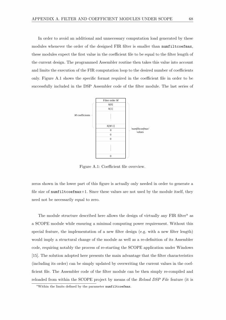
APPENDIX A. FILTER AND COEFFICIENT MODULES UNDER SCOPE 68

In order to avoid an additional and unnecessary computation load generated by these

modules whenever the order of the designed FIR filter is smaller than numfiltcoefmax,

these modules expect the first value in the coefficient file to be equal to the filter length of

the current design. The programmed Assembler routine then takes this value into account

and limits the execution of the FIR computation loop to the desired number of coefficients

only. Figure A.1 shows the specific format required in the coefficient file in order to be

successfully included in the DSP Assembler code of the filter module. The last series of

Filter order M

h [0]

h [1]

h [ M -1]

0

0

0

0

M coefficients

'numfiltcoefmax' values

Figure A.1: Coefficient file overview.

zeros shown in the lower part of this figure is actually only needed in order to generate a

file size of numfiltcoefmax+1. Since these values are not used by the module itself, they

need not be necessarily equal to zero.

The module structure described here allows the design of virtually any FIR filtera as

a SCOPE module while ensuring a minimal computing power requirement. Without this

special feature, the implementation of a new filter design (e.g. with a new filter length)

would imply a structural change of the module as well as a re-definition of its Assembler

code, requiring notably the process of re-starting the SCOPE application under Windows

[15]. The solution adopted here presents the main advantage that the filter characteristics

(including its order) can be simply updated by overwriting the current values in the coef-

ficient file. The Assembler code of the filter module can be then simply re-compiled and

reloaded from within the SCOPE project by means of the Reload DSP File feature (it is

aWithin the limits defined by the parameter numfiltcoefmax.


not necessary to re-start the whole application in this case).

The Assembler code programmed in the file GenFir.asm implements a basic FIR fil-

tering module under SCOPE. Besides the straightforward audio input and output, this

module also presents an overflow monitoring flag output. As mentioned in Section 4.4, a

proper scaling of the FIR coefficients strongly reduces the likelihood of computation over-

flows during the execution of the filter loop. However, in order to obtain a general-purpose

FIR filter module that can be used for any application, this additional flag output has

been also implemented in the code. It is set to a logical 1 whenever one or more multiplier

overflows occurred in the current sampling period.

During the compilation of the Assembler code in GenFir.asm, the coefficient values

are downloaded from the file fircoefs.dat, which is expected to present a format similar

to that depicted in Figure A.1.

A.2 Dynamically Updatable Filters

As highlighted in Section 5.1.1, one of the goals of the work presented in this thesis was

to develop a fully functional system allowing the user to easily design, test and compare

different beamformer types. The Matlab function BDIgui.m presented in Appendix B has

been implemented in order to provide a quick way to accomplish the first part of this task,

that is the design and simulation of the desired beamformer, as well as the computation

of the needed FIR coefficients.

The second part of this task regarding the test and compare side has been implemented

with the help of the SCOPE system. One of the main problems encountered was to find a

way of smoothly updating the beamformer characteristics, and therefore the coefficients of

the FIR filters within the SCOPE project. As described in Section 5.1.1, the solution of a

double buffering of the filter coefficients has been chosen for the Assembler programming

of these FIR filter modules. This section describes various other considerations taken

into account during the development of the filter modules used in conjunction with the

microphone array.


A.2.1 The Filter Module

The module described in this section is obtained from the compilation of the Assembler

code contained in the file FiltMod.asm. It presents a functional principle similar to that

of the module GenFir.asm, which has been briefly described at the end of Section A.1.

This latter has been simply updated with new input and output pads, including especially

a new input labeled CoeffsIn that can be used to download the new FIR coefficients into

the filter module.

As described in Section 4.2.2, the program code of a SCOPE module is divided into two

main routines used for the processing of synchronous and asynchronous data respectively.

The downloading process of the new coefficients into the filter module has been typically

implemented using an asynchronous protocol, due to the non-time-critical nature of this

task. The new values are simply transmitted serially to the filter module which receives

them whenever the execution of its synchronous routine is terminated for the current

sampling period.

In order to allow a “single-wire” transmission in the SCOPE project, this communica-

tion process is initiated by first sending a specific sequence of start values to this module,

which constantly scans its CoeffsIn input pad in order to detect these ignition values.

When such a sequence has been received, it then begins to read the values corresponding

to the new filter impulse response and writes them into the coefficient buffer that is not

currently used in the synchronous routine.

In order to monitor the internal state of this filter module, a series of additional inputs

and outputs have also been implemented besides the audio signal pads. These are described

below.

1. Outputs:

UsedSet: flag set to a logical 1 or 0 depending on which coefficient set is currently

used in the FIR filter computation loop.

LastUpdatedSet: flag set to a logical 1 or 0 depending on the coefficient buffer that

was last updated with new values. The initial value of this flagb is equal to −1,

bI.e. when the module is loaded into the SCOPE project.


indicating that no valid coefficients have been downloaded into either of the

two buffers yet.

MultOverflow: flag set to a logical 1 whenever one or more multiplier overflows

occurred during the FIR filter computation loop.

2. Inputs:

SwapRequest: a falling edge signal applied to this input can be used to arbitrarily

change the coefficient set used for the filter computations.

These different input and output pads have been typically connected to the corre-

sponding displays and buttons of the surface created for the general beamformer project

shown in Figure 5.1.

As already mentioned in Section A.1, the Assembler code of this module also makes use

of the user-definable parameter numfiltcoefmax, which allows to determine the maximum

DSP memory space reserved for the storage of the coefficients.c If this design parameter

needs to be modified, it must be done in accordance with the limits determined by the

number of available synchronous cycles and memory locations in each DSP, as specifically

described in Section 5.1.2.

A.2.2 The Coefficient Module

The module created from the Assembler code CoefMod.asm is the complementary part

of the filter block described in the previous section. This coefficient module presents a

series of outputs corresponding to the total number of filter blocks defined in the SCOPE

project. Each one of these outputs can be simply connected to the CoeffsIn input of the

corresponding filter, allowing a transmission of the new FIR coefficients on the basis of

the asynchronous protocol described in the previous section.

The module defined in CoefMod.asm expects the new coefficient values to be given

in a data file labeled filtbank.dat, where the impulse responses of the different filters

can be simply written one after the other according to the format depicted in Figure A.1.

The parameter corresponding to the current filter length is only needed once at the very

beginning of this file though.

cAnd hence also determines the maximum order of the filter implementable with this module.


The Assembler code developed for this module also allows a change of the parameter

numfiltcoefmax, which corresponds here to the total number of FIR coefficients down-

loaded into each filter module. Furthermore, the additional Assembler parameter numfilt

is used in this code to determine the number of filter blocks that need to be updated

in the SCOPE project. By modifying this value and re-compiling the Assembler code, it

is possible to generate a similar coefficient module with a different number of outputs.

However, care must be taken to ensure that the number of locations reserved this way for

the coefficientsd does not exceed the total memory space available in a single DSP.

This Assembler program has been developed in such a way that the coefficient module

will first update the different filter blocks with the new FIR coefficients, and then enter an

infinite idle state. Hence, a new coefficient download process can be initiated at any time

by means of the Reload DSP File feature provided by the SCOPE DSP Dev. application.

A.3 Summary

The two modules defined in CoefMod.asm and FiltMod.asm, and presented in this chapter

of the appendices have been developed in order to allow a dynamic and parallel update of

the filtering characteristics of one or more FIR blocks present in a SCOPE project. To this

end, the user simply has to overwrite the coefficient values defined in the file filtbank.dat,

after which the Assembler code of the corresponding module CoefMod.asm can be re-

compiled in order to make the new impulse responses available to the SCOPE system.

Finally, by using the Reload DSP File command on the coefficient module in the SCOPE

project, the new FIR coefficients are then automatically downloaded into the different

filter modules, filling the coefficient buffer not currently in use in the filter computation

routine (double buffering). The user can then arbitrarily decide when the new FIR design

should be considered by applying a falling-edge signal to the SwapRequest input of the

different FiltMod.asm modules.

The first two tasks of this filter update processe are automatically carried out by the

Matlab function BDIgui.m. The reader is referred to Appendix B for more information

concerning this beamformer design tool.

dCorresponding roughly to the parameter numfiltcoefmax multiplied by the numfilt value.eI.e. the computation and storage of the new coefficients in the data file filtbank.dat, as well as the

re-compilation of the corresponding CoefMod.asm module.

Appendix B

Beamformer Design Interface

Based on the beamforming theory presented in [1], the Matlab function BIDgui.m has been

programmed in order to provide the user with a tool allowing the easy design and quick

development of different beamformer types for the SCOPE system. It actually represents

a summary of the different principles presented in this thesis and has been created on

the basis of the theoretical developments of Chapter 2 and filter design considerations of

Chapter 4 and Section 5.1.

Figure B.1 presents a general overview of this specific Matlab interface and will be

referenced throughout this appendix section, which describes in detail its two main design

parts, namely the low-pass filter and the beamformer areas.

B.1 Low-Pass Filter Section

The low-pass filter design area is located on the left-hand side of the user interface depicted

in Figure B.1 and it allows the development of a linear-phase FIR filter using a least-squares

error minimization process, as described in Section 4.3.4. The user has the possibility to

adjust a number of settings regarding this low-pass design as described below.

Number of Coefficients: used to determine the desired order of the resulting FIR low-

pass filter.

Attenuation SB: defines the minimum attenuation in dB in the stop-band of the filter.

Ripple PB: defines the maximum desired pass-band ripple in dB.

Frequency PB: desired cut-off frequency of the low-pass filter.

AP

PE

ND

IXB

.B

EA

MFO

RM

ER

DE

SIG

NIN

TE

RFA

CE

74

0 0.5 1 1.5 2

x 104

−140

−130

−120

−110

−100

−90

−80

−70

−60

Am

plitu

de [d

B]

Sensor nr.7

0 50 100 150 200 250

−2

−1

0

1

2

3

4

x 10−4

Am

plitu

de

Blue: real scaled quantized / Red: imaginary

0 500 1000 1500 2000 2500 3000 3500 4000

−110

−100

−90

−80

−70

−60

Frequency [Hz]A

mpl

itude

[dB

]

0 500 1000 1500 2000 2500 3000 3500 4000

−150

−100

−50

0

50

100

150

Frequency [Hz]

Pha

se [d

eg]

20 40 60 80 100 120 140 160 180 200

0

0.02

0.04

0.06

Am

plitu

de

LPF characteristics (200 coefficients, scaled and quantized)

0 0.5 1 1.5 2

x 104

−50

−40

−30

−20

−10

0

Mag

nitu

de [d

B]

0 0.5 1 1.5 2

x 104

−2500

−2000

−1500

−1000

−500

0

Frequency [Hz]

Pha

se [d

eg]

Figu

reB

.1:G

raphical

user

interface

forgen

eralbeam

former

design

.

APPENDIX B. BEAMFORMER DESIGN INTERFACE 75

Frequency SB: frequency from which the specification for the stop-band attenuation

should be met.

By clicking on the button labeled Compute Filter, the low-pass FIR design is realized

according to the various parameter values entered by the user. As a result of this compu-

tation process, the different characteristics of the low-pass filter in the time and frequency

domains are then plotted in the three axes located above the parameter configuration

panel.

Compilation of the Filter Module

The low-pass filter developed within this section of the interface can be typically imple-

mented as a SCOPE module by means of the file GenFir.asm (see Section A.1). In order

to make the resulting FIR coefficients available to this module, they must be written first

into a specific data file (like e.g. fircoefs.dat) that will be then processed during the

compilation of the filter module. The function BIDgui.m has been programmed to auto-

matically scale, quantize and translate the resulting filter coefficients into a format directly

usable for this process by the Assembler compiler. These values are then written into the

data file given by the user in the field Filter Bank File, and the corresponding filter module

(given as Filter Module File) is finally re-compiled by the BIDgui in order to update its

code with the new filter characteristics. The full access path of the directory containing

these two specific filter files must also be passed to the Matlab function via its interface

by the user.

In order to ensure a successful completion of this compilation process, several other

system files must be also present in this working directory. These include notably the files

m.bat and mnot.bat, as well as different other files required for the specific compilation

of SCOPE modules (encryption, translation files, etc., see folder Include in Section F.2).

During the final stage of its compilation, the filter module will be encrypted with the

help of the program cryptdsp.exe (see [15] for more information). This special process

requires a hardware key attached to the serial port of the computer, which also limits

the total number of encryptions available to the user before a new hardware key must

be ordered from CreamWare Datentechnik. Since this number of “crypts” seems to rep-

resent such a sensitive resource, the user is specifically asked to allow this encryption


during compilation by enabling the option Crypting Enabled.a Resulting from the compi-

lation process with this option enabled, the status line of the BIDgui will provide some

information regarding the total number of encryptions left on the current hardware key.

B.2 Beamformer Section

The area reserved for the various beamformer settings and results occupies the main part

of the design interface on the right-hand side of Figure B.1. As already mentioned in the

introduction of this appendix, this section allows the development of a beamformer based

on the model presented in [1]. The user-definable parameters listed below are corresponding

directly to those presented in this reference as well as in Chapter 2, and are not explained

any further in this section.

N: number of modes considered for the beamformer design.

L: minimum number of sensors needed per one array side.

Q: number of uniformly spaced sensors on one side of the array.

Focusing radius: focusing distance in meters from the array origin.

fl, fu: design frequency range of the beamformer.

The function BIDgui computes an FIR approximation of the different sensor filters

using the first variant of the frequency sampling method as described in Section 4.3.2.

The following parameters are available to the user in order to control this FIR filter

design.

Number of coefficients: desired order of the resulting sensor filters implemented with

an FIR approximation.

ffir,l, ffir,u: frequency range considered for the FIR design, defining where the ideal filter

transfer function will be sampled (frequency sampling method).

τobs: this parameter is used in conjunction with the group delay correction that needs to

be accomplished in order to optimize the response of the resulting FIR approximation

(see Impulse Response Only feature later in this section).

aNote that in order to generate a fully functional SCOPE module, this option must be enabled.


The additional parameters fop,l and fop,u provide the user with a possibility to define

the alternate frequency rangeb in which the beamformer is going to be operated. These

variables also define the frequency range used for the different plots of the beamformer

response.

During the computation of the sensor filters, the area labeled Beamformer Info pro-

vides some important characteristics regarding the current beamformer design, like e.g.

the array length or the values L and Q theoretically required according to the different pa-

rameters defined by the user. Of particular importance is the parameter Current τ which

is also displayed in this text field (below the label Beamformer Info). This value gives an

approximation of the group delay of the FIR filter currently plotted on screen and can

be directly entered in the τobs parameter field in order to correct the group delay of the

different sensor filters (see Impulse Response Only feature below).

Sensor Filters Characteristics

Computing the whole beamformer response from the sensor filters with BIDgui.m is a

relatively time-consuming process and is not required as long as the parameters of the

FIR approximation are not completely optimized. By using the button Impulse Response

Only, only the characteristics of the sensor filters and their FIR approximation will be

computed. The execution of the function BIDgui will be then automatically terminated

after having plotted these results instead of going on with the computation of the overall

beamformer response.

This feature allows the user to investigate an FIR filter design resulting from a specific

setting of the parameters, and to quickly correct it if required without having to wait until

the whole “non-ideal” beamformer is computed and eventually plotted.

By means of the “tick-box” Group Delay Correction, the further option is given to the

user to determine whether a correction of the group delay of the sensor filters must be

carried out or not. By un-ticking this box, the impulse responses of the different sensor fil-

ters will be plotted as obtained from the FIR approximation method (frequency sampling

technique) without modification of their phase functions (as described in Section 4.3.4).

bTheoretically equal to the design band, that is from fl to fu.


By observing the different group delays resulting this way in each impulse response (Cur-

rent τ in the Beamformer Info text field), an average value for all the sensor filters can

be determined. This observed average value can be then directly entered into the τobs

parameter field, which will be used by the function BIDgui to automatically compute the

exact phase correction term to use in order to optimize the group delay of the resulting

FIR filters.

Beamformer Computation

After having found an optimum setting of the different user-definable parameters, the

overall beamformer response can be finally computed and plotted by clicking on the button

labeled Compute Beamformer. When doing so, the tick-box Plot Filters can be used to

disable the plots of the different sensor filters if these are not required or in order to speed

up this process. If this option is enabled, the plot area in the beamformer section (upper

right corner of the interface) will show the results obtained for each sensor filter one after

the other, presenting namely the responses in the time and frequency domains. Following

these individual plots, the ideal and practical responses of the beamformer are depicted

in the considered operating frequency range, together with the plots of the theoretical

and practical frequency-invariant beampattern. Finally, the last plot shows the overall

beamformer response over the whole Nyquist frequency range.

These three results are plotted in three different sets of axes which can be individually

displayed on screen after the completion of the computations by means of the tick-boxes

in the upper left corner of the beamformer settings panel.

When computing the whole beamformer response, the feature Use LPF allows the

optional convolution of the sensor filters with the impulse response currently displayed in

the low-pass section of the interface. If the user decides to combine these two filter responses

together, the further Truncate option allows the reduction of the resulting convolutions to

a variable number of coefficients.

In order to speed up the drawing process for the different results, the option Resolution

at the top of the beamformer design panel allows a variable setting of the accuracy of

the plots. The value given in this parameter field corresponds in fact to the number of

frequency points added for the plots in between each frequency location sampled for the


FIR approximation of the sensor transfer functions (frequency sampling method).

Compilation of the Sensor Filters

The button labeled Compile Beamformer on the user interface allows the compilation of

the sensor filters based on the same principle described previously for the low-pass section.

The main difference here is that the BIDgui stores the FIR coefficients of all the

resulting sensor filters in a single data file, ready to be used then for the compilation of a

coefficient module similar to the CoefMod.asm described in Section A.2.2.

B.3 Common General Features

A few features are common to both the low-pass and beamformer design areas of the

BIDgui interface, or are working according to the same principle. For example, the different

resulting plots can be all either rotated or zoomed in and out, depending on whether a two

or three dimensional graph is considered. Zooming in or rotating a figure is initiated by

simply clicking down and dragging the mouse cursor on the considered plot, while zooming

out is performed by a simple click on it.

The Save and Exit button implements a simple way to store the different user-definable

parameters of the interface until a next session, where these settings will be automatically

restored. If this is not desired, the BIDgui figure can be simply closed by means of the

usual Close button in the upper right corner of the window.

The Status line at the bottom of the interface is used to display some important

information regarding the current computation process as well as various error messages

in case of problems. The user should regularly have a look at this text field in order to be

aware of the current state of the function BIDgui.

Special Parameters

Some special parameters of the beamformer design need only be changed or altered in

some rare circumstances. This is the case for example for the Matlab variable fsamp,

which defines the sampling frequency of the digital audio stream. This value must be

set in accordance with the SCOPE project that is going to make use of the different

filter modules developed with the function BIDgui.m. Likewise, the Matlab parameters


numfiltcoefmaxLPF and numfiltcoefmaxc must always be in keeping with the corre-

sponding values defined in the Assembler code of the modules that are automatically

compiled from the BIDgui interface. These two parameters represent the maximum num-

ber of coefficients implementable with the different FIR filter modules programmed under

SCOPE (see Appendix A for more information).

These three special parameters are to be modified only with a complete understanding

of their interactions with the different modules used in the SCOPE project of the beam-

former. Consequently, their value can be accessed and modified only by editing the Matlab

code implementing the function BIDgui.

B.4 Other Useful Matlab Function

The development tool BDIgui.m provides the user with an easy way of downloading the FIR

coefficients of a new beamformer design into the different filter blocks of a SCOPE project.

However, some specific DSP applications require the implementation of a single custom

FIR module under SCOPE. The Matlab function SCOPEcompile.m has been implemented

in order to be able to create such a filter block from an arbitrary impulse response obtained

with Matlab. This custom function is defined as follows:

function [] = SCOPEcompile(FIRCoefs,WDir,ASMFile,DATFile, ...

ScaleCheck,CryptCheck)

This function accepts several parameters that are identical to those defined on the

BDIgui interface. This is the case for the variables WDir, ASMFile and DATFile, represent-

ing respectively the working directory, and the .asm and .dat files that have to be used

for the compilation of the SCOPE module. The input parameter CryptCheck can be used

to enable or disable the encryption of this module as well.

The input variable FIRCoefs defines a vector of values corresponding to the desired

FIR impulse response, which can be additionally scaled if desired (by setting ScaleCheck

to a non-zero value).

cDefined respectively for the low-pass filter and the sensor filters.


B.5 Conclusion

The Matlab function BIDgui.m described in this appendix represents an ideal tool for the

development of a beamformer based on the theory presented in this thesis. With the help

of this user interface, the complete implementation of such a beamformer under SCOPE

comes down to three simple steps only, as described below.

1. Development and simulation of the desired beamformer design with the Matlab

function BIDgui, as described in this appendix.

2. When a desired setting of the design parameters has been found, the different filter

modules can be compiled from the BIDgui interface by clicking on the Compile

Beamformer (respectively Compile Filter) button.

3. Finally, the FIR coefficients (and consequently the whole beamformer design) can be

updated in the SCOPE project by simply making use of the Reload DSP File feature

on the concerned filter modules (see Appendix A and [15] for more information

concerning this process).

Appendix C

Signal Gain Calibration

The use of the hardware tools at disposal and described in Chapter 3 does not allow an ac-

curate gain adjustment for the different microphones used in the array. More importantly,

it is practically not possible to ensure that all the signal paths of the different sensors

present the same overall gain. A signal calibration must therefore be implemented in soft-

ware in order to make sure that the gain difference from one signal to another is not too

significant and will not induce a noticeable degradation of the beamformer functionality.

This chapter of the appendices deals with a specific SCOPE module that has been

developed to this purpose. It first presents the theoretical principle used to accomplish

this calibration. According to this method, the results obtained from a Matlab simulation

performed with a real microphone input signal are then depicted in a second section.

Since the Matlab function developed for this simulation is needed in the final calibration

process, its different inputs and outputs are also described with more details. Then follows

a full description of the SCOPE module itself and of its different parameter settings

and working principles. To sum up, the last section of this appendix presents a complete

method that can be followed step-by-step to calibrate the different signal paths of an array

of microphones.

C.1 Calibration Principle

The basic idea of such a calibration was to use a “stable” sound source emitting in the

vicinity of the sensor under test and to adjust a software gain in the SCOPE project

according to a pre-defined specification to satisfy for the modified signal. The next sensor

can then be placed at the exact same location and its corresponding gain adjusted so that

APPENDIX C. SIGNAL GAIN CALIBRATION 83

the same specification is met again.

Several different sound sources and methods have been studied and tested in order to

obtain an accurate gain adjustment under SCOPE. The best results for this calibration

have been achieved with a white noise sound source. A random signal literally excites all

modes in a room and generates a more regular and stable acoustic field than other sound

sources, like for example a single frequency tone [40]. The average power of the recorded

signal is then computed and a basic PID controller (see e.g. [43, 44]) is used to adjust

the corresponding signal gain until a pre-defined power level is reached. Figure C.1 shows

a block diagram representing the calibration principle developed for the practical tests

described in this thesis.

i K

+

+

+

p K

d K

Random Noise Generator

?

G

Sensor under calibration

Input signal of unknown power

Gain G

Output signal with desired

power

Current signal power

C P D P

1 S 2 S

Error +

_

PID Controller

“Plant”

Desired signal power

T

1 T

0

( ) dt 2 .

( ) dt .

d ( ) . dt

Figure C.1: Microphone calibration principle.

According to [28], the power of a digital signal X[n] is equivalent to its variance σ2X .

For a zero-mean stationary gaussian process like white noise, this value can be computed

according to Equation C.1 (see [41]), which will be used in the following instead of the

continuous-time formula given in Figure C.1.

σ2X =

1

N·

N∑

n=1

X2[n] . (C.1)


Figure C.1 represents a unity feedback system comprising a “plant” driven by a con-

troller. In our case, this plant consists of the adjustable gain G influencing the level of

the input signal S1, and a unit computing the power PC of the resulting signal S2. This

value is then fed back to determine the tracking error, that is the difference between the

desired power value PD and the current signal power PC . This error function constitutes

the input of the controller, which in turn adjusts the gain value G so that the error func-

tion progressively decreases to zero. Figure C.1 also shows the internal working principle

of the PID controller, consisting of three different paths with parameters Kp, Ki and Kd

respectively. The characteristics and effects of each of the proportional (P), the integral

(I), and the derivative (D) controls are summarized as follows (see [45, 46]).

The proportional control (Kp) will have the effect of reducing the rise time and will

reduce, but never eliminate, the steady-state error.

The integral control (Ki) will have the effect of eliminating the steady-state error, but

it may make the transient response worse.

The derivative control (Kd) will have the effect of increasing the stability of the sys-

tem, reducing the overshoot, and improving the transient response.

It must be noted here that these correlations may not be exactly accurate, because the

parameters Kp, Ki and Kd are dependent of each other. In fact, modifying one of these

variables can change the effects of the other two.

From a quick consideration of the block diagram given in Figure C.1, it can be seen

that an open-loop unit step response of the “plant” would present a negligible rise time

and overshoot, but will show a relatively consequent steady-state error (depending on the

actual input signal power). Consequently, the most significant parameter to consider is

the gain Ki of the integral path, which will help eliminate completely this kind of error.

The other two parameters Kp and Kd are of lower importance for this controller design.

C.2 Controller Simulation with Matlab

Prior to the implementation as a module under SCOPE, the calibration and controller

principles presented so far have been simulated and tested with a real signal recorded from


within the SCOPE application. Figure C.2 shows the results obtained with the specifically

developed Matlab function PIDcal.m using a 150 second white noise sample. The com-

putation of the different signal power values is done according to Equation C.1 over 30

periods of 5 s duration each.

0 50 100 150

0

0.02

0.04

0.06

0.08

Power Functions (Input and Calibrated Signals)

Time [s]

0 50 100 150

0

0.2

0.4

0.6

0.8

Controller Values

Time [s]

Gain I−Part

P−Part

D−Part

Figure C.2: Simulation of the PID controller forgain calibration purposes.

The upper part of Figure C.2 shows the relatively constant power of the input white

noise signal, as well as the power progression of the resulting calibrated signal. The lower

plot shows the different internal controller values, as well as the resulting gain. As this

gain value is progressively adjusted by the controller, it can be seen that the power of the

resulting signal eventually reaches a steady-state corresponding to the pre-defined desired

power (grey line in the upper plot), set in this example to 70% of the average power of the

input signal. These plots are resulting from a controller parameters setting of 1, 3 and 0

for Kp, Ki and Kd respectively. A faster settling time than that depicted in Figure C.2 can

be obtained by further increasing the value for Ki, resulting in an even faster calibration

process.

The lower plot also allows to make sure that all the internal controller signals are rep-

resentable in the DSP two’s-complement format.a This fact also implies another important

restriction for the calibration process: since the signal gain G is restricted to a value smaller

than one and consequently can only implement an attenuation, it is necessary to specify

the desired signal power value smaller than the average power of the current

input signal.

aI.e. comprised in the range[−1 . . . 1 − 231

].


It can be seen from Figure C.1 that the efficiency of the PID controller, and especially

its convergence time, strongly depends on the power of the actual input signal. Since this

power value will usually differ from one calibration process to another, it is good practice

to check the different controller settings first with a software simulation prior to starting

the actual calibration of the microphones under SCOPE. This guarantees a satisfactory

controller behaviour with fast settling time and no oscillation errors. The Matlab function

PIDcal.m can be used to this purpose and its working principle will hence be described in

detail in the following.

Matlab Simulation Function

The file PIDcal.m contains a custom Matlab function defined as follows:

function [] = PIDcal(Kp,Ki,Kd,NrAvVal,Perc,IntTime,WavFile)

and accepts the different parameters described below.

Kp, Ki, Kd: correspond to the respective PID controller parameters.

NrAvVal: the function PIDcal offers the possibility to average the final PID gain over a

variable number of values following the moment when the power of the controlled

signal reaches the desired level (after a settling time of approximately 60 s in the

example given in Figure C.2). The parameter NrAvVal corresponds to the desired

number of values to consider for this average.

Perc: defines the desired power level as a percentage of the input signal power. This value

must be given as a fractional number comprised between 0 and 1.

IntTime: integration time in seconds to consider for the computation of the different signal

power values (corresponds to the value N in Equation C.1 divided by the current

sampling frequency).

WavFile: file name of the desired white noise sample with full access path.

More information can be obtained by calling the on-line help text for this function

from the Matlab command prompt (e.g. by entering help PIDcal).


The result of this function is a plot similar to that depicted in Figure C.2. The Matlab

window will also contain a function output which typically looks as follows:

### Audio sample length: 150.39 [s]

### Number of 5sec. power integration periods: 30

*** Direct signal average power: 178930806

*** Desired Power (70%): 125251564

*** Average resulting gain: 1795504378

First, the function displays some basic results concerning the length or the selected audio

sample and the number of power values obtained from the chosen integration time. The

last three lines give information about the average power of the input sample, the desired

power selected by the user as well as the resulting gain that has to be implemented in order

to match this desired power level. These data are all in a format that is directly usable

with the calibration module developed under SCOPE (see module PIDcal.asm later in

Section C.3).

It is also possible that after the completion of this function, a similar error message

appears:

### PID gain cannot be averaged over the last 5 gain values!

meaning that the controller did not reach a complete steady state before the completion

of the simulation. In this case, the function has to be restarted again with a longer audio

sample or a setting of the controller parameters allowing a faster convergence time.

C.3 SCOPE Calibration Module

The SCOPE module PIDcal.mdl (with source code in PIDcal.asm) has been developed

for the microphone calibration process described in this appendix. It simply consists of the

audio input called AuIn and the output PIDG where the resulting gain of the controller can

be accessed. More important than the module itself though is its surface, which contains all

the controller settings and values resulting from the calibration. Figure C.3 gives a typical

outlook of this module interface. As it can be seen in this figure, this user interface is

subdivided into five main areas. In order to completely understand the working principles

of this module, a detailed description of the different parameters and features available in

each one of them is provided in the following subsections.


Figure C.3: Surface of the sensor gain calibration module.

Power Estimates Section

This section of the surface contains two user-definable parameters used for the computa-

tion of the different signal power values. The input field labeled Computation Time can

be used to enter a value corresponding to the integration time to use for the power com-

putations. This parameter is similar to the variable IntTime of the function PIDcal.m

described in the previous Section C.2, except that it must be given here as the number N

of audio samples to consider for the sum given in Equation C.1.

The module described in this appendix also computes the long-term averages of the

different power values according to the following recursive equation:

PowerAverage[ i ] = α·PowerAverage[ i − 1 ] + (1 − α)·Power[ i ] . (C.2)

This formula corresponds to a moving average where the past values are progressively

attenuated with a rate depending on the chosen factor α, as shown in Figure C.4.


Averaging Function (with Parameter α)

Number of Samples0 10 20 30 40 50

0

0.1

0.2

0.3

0.4

α = 0.95α = 0.9

α = 0.8

α = 0.7 α = 0.6

Figure C.4: Moving average functions.

The surface variable Average Parameter corresponds to the parameter α in Equa-

tion C.2. If the power integration time is set to a relatively high value, it can be seen

that quite a long time must be considered before this moving average process reaches a

steady state. For example, with an integration time of 10 s and an averaging parameter α

set to 0.95, the user will have to wait for a period of approximately 10 minutes before a

relevant power average is obtained with Equation C.2,b according to Figure C.4. Conse-

quently, the Average Parameter is only relevant for relatively small integration time values

(Computation Time).

PID Controller Section

Several input parameters in this section of the surface correspond directly to those used in

the Matlab function PIDcal.m described previously and do not need further explanations

at this stage. This is the case for the parameters Kp, Ki, Kd and Number of Average

Values. The input variable Desired Power corresponds to the used-defined signal power

that should be ultimately reached by the attenuated signal and can be directly imported

from the results obtained from a simulation with the function PIDcal.m (see Section C.2).

The module PIDcal offers the additional feature compared to the corresponding Mat-

lab function that the resulting PID gain is averaged over a certain number of gainsc only

if the resulting signal power is constantly comprised within a tolerance band around the

desired power level. If a computed power value is found to be outside this band, this av-

eraging process is automatically reset and only re-started when the power value lies in

the tolerance band again. This feature avoids corrupted results due to parasitic noises

bAnd this after the controller itself has reached its own steady state as well.cAs defined by the user with the parameter Number of Average Values.


or to oscillations in case the controller has been badly designed. The surface parameter

Tolerance allows the user to define such a value (see Direct Signal Section below to see

how to determine a suitable value for this parameter).

The flag Ready/Calibration done can also be found in this surface subdivision and is

turned on each time a calibration process has been successfully accomplished. The different

results obtained from the PID controller can then be read in the right-hand side fields,

which notably show the final PID gain obtained (same value as the module output PIDG).

The field Number of Iterations shows the total number of power computations that

were necessary during the last calibration. The value labeled Gain Average Counter can

be read during the process; it is equal to Number of Average Values at the beginning of the

calibration, and then decreased each time the resulting signal power is found to be within

the tolerance band around the desired power level. As described earlier, it might also be

reset to Number of Average Values during this gain averaging process if the power value

suddenly jumps out of the tolerance band for some reason. Consequently, the parameter

Gain Average Counter will be equal to zero when the calibration process is over and the

flag Ready is on.

Direct Signal Section

This interface area is giving some basic information about the different characteristics of

the input signal, based on the current settings of the Power Estimates section. The Cur-

rent Power is computed according to Equation C.1 and the Average Power corresponds

to the moving average value defined by the recursive formula C.2. The field ALU Overflow

will show a non-zero value if one or more overflows occurred during the different power

computations. In this case, the calibration results may be corrupted and the whole process

should be re-started again with a lower-level input signal.

The top and middle values on the right-hand side of the surface (Current Maximum

Value and Current Minimum Value) show the respective maximum and minimum results

obtained from the power computations for the current input signal. The last field labeled

(Max-Min)/2 is determined by these two values and gives some information about the

power “variance” of the input signal, which in turn can be used as a reference in order


to determine the Tolerance parameter. If the power of the input signal oscillates with a

maximum amplitude of (Max-Min)/2 around its average, then the resulting calibrated

signal should oscillate around the desired power level with an amplitude smaller than

(Max-Min)/2.d However, since the power of the output signal also depends on the current

value of the PID controller gain,e this relation might not be constantly verified.

Hence, a basic rule of thumb is to set the parameter Tolerance slightly bigger than

the resulting (Max-Min)/2. Such a Tolerance value has proved to provide an accurate

calibration without resetting the gain averaging process too often.

Calibrated Signal Section

This section gives information about the power characteristics of the resulting calibrated

signal, the computation of which is similar to the principles used for the corresponding

direct signal values. After a successful calibration process, the results shown in the two

output fields of this section will be close to the desired signal power given as specification

in the PID Controller area.

General Commands Section

Two more features are provided by the PIDcal module. The first one allows the user to

reset the internal values of the controller to zero, especially the different average power

computations as well as the parameters ALU Overflow, Current Minimum Value, Current

Maximum Value and (Max-Min)/2.

The button on the right-hand side provides a way to “freeze” the different outputs of

the surface for a further analysis. If a calibration is in progress, the different controller

outputs will still be updated, but the surface will enter the frozen mode again as soon as

the calibration is over. This feature is quite practical when using a long power integration

time (and hence a long calibration time): it allows the user to start the calibration in a

stand-alone mode and to come back at a later time to study the results obtained, even

though the calibration process may have terminated in the meantime.

dReminder: the PID gain implementable with the DSPs has a value comprised in the range[−1 . . . 1 − 231

]and is hence smaller than unity.

eThe power of the output signal is equal to that of the input signal multiplied by the squared value ofthe PID gain, see Figure C.1.


In order to provide some more general information about the characteristics of the

input and calibrated signals, two level-meters have also been included on the top right

corner of the surface.

C.4 Calibration Method for an Array of Microphones

Based on the developments presented in this appendix, the method described below has

been used in order to calibrate the different signal paths in the microphone array applica-

tion considered in this thesis.

1. First, a coarse setting of the different “hardware” signal gains can be undertaken to

ensure that all the resulting sensor gains under SCOPE will be in the same order

of size. This minimizes the effects of a variable quantization error due to different

software gain magnitudes.f This can be done by setting all the “volume” knobs of the

pre-amplifier channels to the same position. This unfortunately does not ensure that

the gains are identical from one sensor to the other however, and a better way to

proceed is to use the PIDcal module under SCOPE. By choosing a relatively short

power computation time (e.g. half a second or so), the knob of each channel can be

adjusted by hand so that the Current Power field (or even the Average Power) of

the direct signal is showing a similar result for each sensor.

2. The first sensor under calibration can be placed then in front of the white noise

source and a sample of the signal generated this way in the SCOPE project (typically

originating from a SCOPE ADAT Source module) can be recorded in a .wav file.

3. With the help of this audio sample, the PID controller can be simulated with the

Matlab function PIDcal.m with various parameter settings until a satisfactory con-

troller behaviour is achieved. The controller parameters obtained this way can then

be copied to the corresponding surface input fields of the SCOPE module PIDcal,

also including the desired signal power value resulting from the simulation.

4. By observing the characteristics of the input signal for a few seconds (parameter

(Max-Min)/2 ), an appropriate Tolerance value can be determined as well according

to the basic rule of thumb given in Section C.3.

fThe percentage error produced by truncation or rounding tends to increase as the magnitude of thenumber to represent is decreased, see [27].


5. The calibration can then be started by simply clicking on the corresponding button

of the PIDcal module surface. When this process is finished, the resulting PID gain

value can be stored either from the module output, or by copying it from the surface

field labeled PID Gain.

6. The next sensor can be placed then at the exact same location in front of the sound

source, and after having re-connected the input of the PIDcal module to the new in-

put signal under SCOPE, the calibration process can be restarted again as described

in point 5.

The series of signal gain values obtained from the process described above for the dif-

ferent sensor paths can be implemented finally by using the modules GainBank15 and G15

(with Assembler code in Gain15.asm), which is a module containing 15 parallel multiplier

blocks (see Figure 5.1). These modules can be easily updated and re-compiled to accept a

different number of input signals.

C.5 Results

This appendix has presented a complete way of compensating in software for the hardware

gain difference generally present from one signal path to another in an array of micro-

phones. Two main program codes have been developed to this purpose under Matlab and

SCOPE, and have been described here in detail. The function PIDcal.m constitutes an

ideal way to quickly test the different parameter settings of the PID controller, and the

SCOPE module obtained from the Assembler code PIDcal.asm provides a way to accu-

rately calibrate the sensors. The implementation of the additional Tolerance feature for

this module makes it entirely stand-alone since in case of a calibration disturbance due to

accidental external noise, the whole calibration process is reset and suspended until the

controller reaches a steady state again.

A complete calibration process to follow step-by-step has finally been presented on the

basis of these developments, and has been used successfully for the different microphone

calibrations performed in this work. This method can be used for virtually any signal

calibration task in further projects developed with the SCOPE system.

Appendix D

Room Reverberation

Measurements

This appendix describes the practical setup used to measure the reverberation time RT60

of the testing environments used during the experimental phase of this work. It also

presents and explains the different functions developed with Matlab to easily and automat-

ically determine this value in case the measurements of another room is to be performed

later on.

D.1 Reverberation Time Measurements

When a loudspeaker arranged to emit random noise into a room is switched on, it will

produce a sound that quickly builds up to a certain level. This latter constitutes the

equilibrium point at which the sound energy radiated from the loudspeaker is just enough

to supply all the losses in the air and a the boundaries of the room. When the loudspeaker

switch is opened, it takes a finite length of time for the sound level in the room to decay to

inaudibility. This “hanging-on” of the sound in a room after the exciting signal has been

removed is called reverberation and it has an important bearing on the acoustic quality of

the room.

The characteristic value used in this work to give a basic information about the rever-

beration of a testing room is the RT60 [40]. This value is defined as the time required for

the sound in a room to decay 60 dB, and it can be practically measured as described in

the following. Figure D.1 shows the practical setup used in this work to this purpose.

APPENDIX D. ROOM REVERBERATION MEASUREMENTS 95

Random Noise Generator

Power Amplifier

To the SCOPE system Microphone Pre-

Amplifier

Figure D.1: Equipment for room reverberation measurements.

A loudspeaker is emitting a random signal coming from an amplified white or pink

noise generator, filling the room with a very loud sound. Aiming the loudspeaker into a

corner of the room allows the excitement of all resonant modes (see [40]). A non-directional

microphone is then positioned randomly in the room in order to provide a signal charac-

terizing the resulting acoustic field. By opening the switch, the sound is made to quickly

decay according to the reverberation characteristics of the room. The microphone picks

up this decay and transmits it to the SCOPE system and other applications for further

analysis. In order to determine a better statistical picture of the sound field behaviour in

the room, several such measurements should be accomplished at different positions and

with different bands of random noise.

In order to measure the RT60 of a room according to this principle, the SPL value

(Sound Pressure Level) of the recorded signal can be computed as follows:

SPL [dB] = 10 · log10

(p

p0

)2

, (D.1)

where:

p is the sound pressure in Pascals (typically provided by condenser microphones like those

used in this work),

p0 is a chosen reference pressure (set here to 20·10−6 Pa).

As described in [40], a relatively high background noisea is not a real problem for re-

verberation measurements according to the method described above. The straight portion

aI.e. a poor signal-to-noise ratio.


of the sound decay can simply be interpolated in order to obtain a difference of 60 dB

compared to the average noise level.

D.2 Software Developments

The Matlab function RT60.m has been programmed in order to automatically compute the

reverberation time of a room from a real sample of audio data. The declaration of this

function is as follows:

function [] = RT60(MaxLen,WavFile,IndexVec)

The three parameters expected by this function are described below.

WavFile: a two channel file in .wav format. The first vector must contain the sample of

audio data starting during the noise period and finishing with silence. The second

channel must be a binary signal consisting of a series of non-zero values followed

by a sequence of zeroes, in order to give information to the function concerning the

exact moment at which the noise source has been switched off.

MaxLen: in order to compute an average sound level during the noise and silence periods

respectively, this function determines the SPL envelope of the input signal by taking

one maximum level value in each period of MaxLen samples.

IndexVec: this optional two element parameter defines the start and end indices of the

desired audio sample in WavFile to be considered by this function (call the on-

line help for the built-in Matlab function wavread.m for more information about

this parameter). If IndexVec is omitted, the function wavscan.m (see later in this

section) is called in order to allow the user to define the appropriate limits to consider

in the audio sample for the reverberation measurements.

Figure D.2 shows a typical plot that can be obtained with this custom function. It

is the result of a reverberation measurement performed with white noise in one of the

laboratories in the Engineering Department of the ANU. The next three lines show a

typical output to the Matlab command window presenting the different results obtained

from this function:

### Mean SPL during noise: 90.29[dB]

### Mean SPL during silence: 56.72[dB]

### Reverberation time = 0.85[s] (time period [s]: 1.73...2.58)


Time [s]

SP

L [d

B]

SPLnoise

= 90.3dB

SPLnoise

−60dB

SPLsilence

= 56.7dB

0 0.5 1 1.5 2 2.5 3 3.5 410

20

30

40

50

60

70

80

90

100

Figure D.2: Typical plot resulting from the func-tion RT60.m.

Since the transition between the end of the sound decay and the beginning of the

silence period is generally not clearly defined, the function asks the user to interactively

set these limits on screen (corresponding to the two vertical lines on the right-hand side

of the plot in Figure D.2).

As already shown, this function also allows the computation of the average SPL during

the silence period, giving this way some interesting information concerning the SNR and

dynamic range in the testing environment.

The audio samples recorded from such measurements are usually quite long and me-

mory-consuming. Furthermore, only a small portion of them is of interest from a rever-

beration point of view.b Since the processing of the whole sound sample generally leads to

unnecessarily long computation times, the specific Matlab function wavscan.m has been

programmed in order to allow an easy handling of such audio samples. It provides the

user with a quick way to visually “edit” .wav files and determine the start and end indices

of the portion of interest, which can be then directly passed to the function RT60.m as

the parameter IndexVec. Type help wavscan at the Matlab command prompt for more

information on this custom function and its different features.

To conclude this section, an overview of a typical SCOPE project used for reverberation

measurements is depicted in Figure D.3. The module VolAtten.asm in this project is used

bTypically a period of 2 or 3 seconds around the source stop time.


Figure D.3: Typical SCOPE project for reverberation measurements.

for two different purposes. Via its input Volume, it allows a modification of the noise signal

level produced by the loudspeaker. This volume value can be increased until slightly before

the loudspeaker starts to overload in order to generate the largest dynamic range without

obtaining corrupted results. Furthermore, the noise signal can be suddenly cut by means

of the Mute input of this module for the reverberation measurements.

The resulting signal picked up by the microphone in the tested environment is then sent

to the module Wave Dest 1, which also receives the signal corresponding to the current

state of the sound source (on or off). The .wav file passed as WavFile parameter to

the Matlab functions wavscan.m or RT60.m can be then generated by simply recording the

signal inputs of this module into a single stereo file with the help of a digital audio software

(like e.g. Cakewalk Pro Audio or Cool Edit Pro). The module labeled Async mult integer

is implemented in order to make the change of the noise source state fully detectable for

the Matlab function RT60. The output value of the On/Off button in the SCOPE project

is either 1 or 0 and would not appear in the recorded sample otherwise.


D.3 Octave-Band Analysis

The value returned by the Matlab function RT60 described above constitutes the average

reverberation time over all the frequencies in the spectrum.c In order to obtain an even

better idea of the acoustics of a room, this value can also be computed for different

frequency bands of the input signal. A common practice in the acoustics domain is to

divide the spectrum into separate octave bands with middle frequencies fm, with a fixed

reference frequency fm,0 = 1000 Hz. The relation between the middle frequencies of two

adjacent octave bands is defined as follows:

fm,n+1 = 2 · fm,n .

Likewise, the upper and lower frequencies of the n-th band (respectively fu,n and fl,n)

can be computed from its middle frequency fm,n according to the following equations:

fu,n = fm,n ·√

2 ,

fl,n =fm,n√

2.

According to these definitions, a total of 9 different octave bands have been defined for

the current measurements.d Table D.1 presents respectively the lower, middle and upper

frequency of each one of them.

Results

The new function RT60oba.m has been implemented with Matlab. It presents the same

features as the original RT60.m but has been updated to first process the input sample

with the current octave filter before computing its reverberation time. It hence returns

such a value for each one of the octave bands listed in Table D.1 (see on-line Matlab help

on this function for more information). Figure D.4 shows the different results obtained

with this Matlab function for two different tested environments, namely a general purpose

engineering laboratory room and the newly built anechoic chamber.

A total of 10 audio samples (5 different microphone positions with 2 measurements

each) have been analyzed in the laboratory, the resulting average of which is represented

cLimited practically by the quality of the loudspeaker and the current sampling rate.dFor a sampling frequency of either 44.1 or 48 kHz.


fl fm fu

0 62.5 88.4

88.4 125 176.8

176.8 250 353.6

353.6 500 707.1

707.1 1000 1414.2

1414.2 2000 2828.4

2828.4 4000 5656.9

5656.9 8000 11313.7

11313.7 16000 FNyquist

Table D.1: Octave band frequencies (in Hertz).

by the upper curve in Figure D.4. In the anechoic chamber, 6 microphone positions with

4 measurements each have been used, resulting in 24 different values for each octave

(lower curve). Pink noise has been used for both environments in order to obtain a better

approximation of the reverberation time for the low frequencies.

Frequency [Hz]

Rev

erbe

ratio

n T

ime

[s]

102

103

104

0.1

0.2

0.3

0.4

0.5

0.6

0.7

0.8

0.9

1

1.1

Figure D.4: Reverberation time measurementswith octave-band analysis.

The results depicted in Figure D.4 show the distinct acoustic improvement offered for

the tests in the anechoic chamber, which presents an average reverberation time below

0.1 s for frequencies above 400 Hz.


An interesting acoustic behaviour in the anechoic room has been observed when com-

puting its reverberation time for the different octave bands. Figure D.5 gives an exam-

ple of such a measurement, corresponding to the octave band centered on the frequency

fm = 1000 Hz of a pink noise sample.

Time [s]

SP

L [d

B]

SPLnoise

= 72.6dB

SPLnoise

−60dB

0 0.2 0.4 0.6 0.8 1 1.2 1.4

0

10

20

30

40

50

60

70

80

90

Figure D.5: Reverbatory decay with doubleslope.

In this example, one can distinctly notice two different slopes during the noise decaying

period, which is a result typically obtained for acoustically coupled spaces (see [40]). The

anechoic chambere presents three ventilation openings in its walls that have not been

completely covered, thus acoustically coupling it with the outside room it has been built

in. This in turn generates a noise decay as that depicted in Figure D.5. The shorter

reverberation time in this plot, represented by the first slope (black line), corresponds to

that of the anechoic room. The second slope represents the noise decay in the acoustically

coupled room. With these measurements, the shape of the reverberation decay has pointed

to this particular acoustical problem, which is most probably going to be solved in the

future.

ePreviously a radio frequency shielded room.

Appendix E

SCOPE “Troubleshooting”

One of the drawbacks of the SCOPE system is that when an error occurs in the project or

a module does not work properly, there exists no specific way to determine exactly what

causes the problem. Even the different error prompts appearing sometimes in the SCOPE

software usually fail to point out where the problem is really coming from. It is then not

uncommon to have to spend a relatively long time trying to track down the code error to

eventually be able to correct it.

This appendix aims to give some help with different error types that have occurred dur-

ing the development of the SCOPE modules required for the work presented in this thesis.

It gives a list of the most frequent problems encountered and the possible errors causing

them. It also gives some basic rules to keep in mind when programming in Assembler for

the SCOPE DSP Dev. application.

However, the information given in this appendix is generally the result of a trial and

error process used to debug a program code. Therefore, this section does not pretend to

provide an exhaustive list of all the different problems that may arise and of their solution.

It can be used however in order to get an idea concerning different kind of programming

errors that are more likely to be made and what symptoms they generate under SCOPE.

The solution of a problem related to a custom module not behaving correctly under

SCOPE is to be found exclusively in the Assembler code that has generated it. In relation

with this code, two main types of programming error can be defined:

1. Errors related to the Assembler language itself and to the compiler used to generate

the opcode for the DSPs.

APPENDIX E. SCOPE “TROUBLESHOOTING” 103

2. Errors related to the specific way the code is interpreted by the SCOPE system, and

to the different restrictions implied by this system on the development of Assembler

programs.

This appendix is subdivided into two different sections discussing these two different

subjects. It is furthermore assumed here that the reader possesses a certain background

knowledge concerning the Assembler language and the SCOPE application.

E.1 SCOPE Related Problems

The most important thing to keep in mind when programming in Assembler for the SCOPE

DSP Dev. is to always adopt a rigorous programming: a single flag set to a wrong value can

make the whole application crash without notice when trying to use the created module.

The developer should therefore always be aware of all the different programming subtleties

described in the user’s manual of this product [15]. Below is furthermore a list of the most

common problems encountered during the work presented in this thesis.

1.) Symptoms: when trying to load or re-load a module under SCOPE, the following

error messages appear on the screen:

Timeout waiting for acknowledge from DSP0. Do you want to reload the DSPs?

and:

Unexpected DSP overload: increase the SafetyCycles setting in CSET.INI and

restart SCOPE or try reloading the DSPs using the current settings.

Solutions: these error prompts probably appear as a consequence of different types of

error. In this work however, this problem was generated by a buffer of variables declared

with the .var directive before the synchronous routine in .segment /pm seg-sync. In

case a variable or buffer has to be defined in the program memory of a DSP, it can be

done in this segment but the buffer must be defined after the end of the synchronous

routine.

2.) Symptoms: some sort of double buffering problem occurs in the synchronous outputs,

for instance an output appears sometimes on the display of the previous one; or the

synchronous procedure simply does not seem to return meaningful results.


Solutions: due to the specific way the SCOPE system handles the communication of

synchronous data from one module output to another module input, it is important to

update all synchronous outputs of a module during each call of the synchronous routine,

even though these values may not have been modified.

3.) Symptoms: some outputs of the created module are working correctly, and some

other are not; or the SCOPE application crashes when trying to connect a module pad to

another module.

Solutions: the line .var flags=0 was missing in .segment /dm seg-desc, which was

producing the fatal error. Also, the blank spaces in the different pad names were removed,

which probably contributed to the success of the debugging as well.

4.) Symptoms: the input of a module expecting a rising or falling edge signal regis-

ters several hundred changes each time such an event occurs when this trigger signal is

generated for instance with the “On/Off” button under SCOPE.

Solutions: the cause of the problem could not be precisely determined. However, a specific

module (with Assembler code in AG.asm) has been implemented in order to avoid these

parasitic impulses in the input signal. This module presents one input and one output.

Each time a change of the input state is detected, the output is modified accordingly,

following which a counter is started and prevents the output to change again during a

certain number of cycles. The value of this counter can be easily modified by editing the

file AG.asm.

5.) Symptoms: an output displayed on a Text Range shows a correct value and then

changes to zero whenever the user clicks somewhere else in the SCOPE project.

Solutions: here again, this odd behaviour still remains somewhat obscure, but this prob-

lem could be fixed by switching the SCOPE application to Move Mode (see [14], where

the output of the module was constantly showing a correct value.

6.) Because of the way the SCOPE handles the different segments of the program code,

care must be taken when handling variables declared in certain segments that are not

loaded only once for all instances of the same module in the project. For example, if a


buffer is defined in program memory together with a pointer variable, it is not possible to

initialize this pointer value as follows:

.segment /pm seg_sync;

sync: ...

[synchronous routine code]

...

JUMP ret_sync; // End of sync code.

.var buffer[512];

.var bufpointer = buffer; // Doesn’t work!

.endseg;

The value in bufpointer will not point onto the base address of buffer because during

compilation, it is not known exactly where the segment .segment /pm seg-sync will be

located in the DSP memory. Consequently, the base address of the variable buffer is not

determined at this stage either. The only way to go round this problem is to initialize

the pointer in .segment /pm seg-init, which is executed each time the module code is

loaded into a DSP. As an example, the following statements could be used instead:

.segment /pm seg_init;

init: I8 = buffer;

// I8 loaded with base address of "buffer".

PM(bufpointer) = I8;

// "bufpointer" now points onto "buffer".

RTS;

.endseg;

E.2 Assembler Language Hints

The development of program code in Assembler language is made by using a relatively

small set of pre-defined commands. The only way to ensure a correct programming of

the desired routines is hence to fully understand the syntax related to this programming

language as described for example in [13, 11]. The following list only gives a few important

points that a first programmer may be unaware of, and which may lead to misbehaving

SCOPE modules.

1.) The Assembler compiler does not handle correctly zero-length buffer declarations. For

instance the expression

.var asyncOut[2*ASYNCOUT];


will not be compiled correctly if the variable ASYNCOUT is set to zero, in which case this

line must be removed or put in comments instead.

2.) The Assembler compiler is case sensitive. Hence be sure to write for example syncOut

and not syncout, otherwise the module will not work properly. Also, the compiler does

not manage filenames and labels with more than 8 letters in it, which can lead to serious

problems if the some of the code labels or variables begin with the same 8 letters.

3.) The compiler can only evaluate one symbol in each expression. If for instance the two

variables are defined in the code as follows:

#define val1 5

#define val2 4

then the Assembler command R0 = val1+val2 is not executed correctly. A single symbol

expression must be found instead.

Appendix F

CD Contents

A data CD is included with this thesis in order to make the most important files developed

for this work available to any other person willing to use them. This appendix gives a brief

overview of the different files contained in this CD together with a short explanation of

their respective function. If a more detailed description has been already provided in a

previous section of this thesis, a reference to this section is given instead.

F.1 Matlab Files

BDIgui.m: graphical user interface for the development and simulation of different types

of beamformer, see Appendix B.

BDI2.m, BDI2.mat: machine-generated files for the representation of the Matlab figure

used by the function BDIgui.m. Note: these files must be present in the Matlab path

when calling the function BDIgui.m.

PIDcal.m: program simulating the behaviour of a PID controller used in order to calibrate

the gains of different microphones, see Appendix C.

RT60.m: functions used to measure the reverberation time of a room from a recorded audio

sample, see Appendix D.

RT60oba.m: same function as RT60.m updated for an octave-band analysis of the input

sample, see Appendix D.

SCOPEcompile.m: function allowing to compile an arbitrary FIR filter impulse response

and to download it into any SCOPE filter module, see Section B.4.

APPENDIX F. CD CONTENTS 108

wavscan.m: allows a visual “editing” of an arbitrary audio sample, see Section D.2.

wavTF.m: automatically determines the frequency response of an unknown system over a

desired band from a general .wav file, see Section 5.3.1.

Folders

AudioSamples: this folder contains several example samples of different audio signals

that can be used for demonstration purposes in conjunction with the different Matlab

functions mentioned above. For some of these functions, the Matlab on-line help

contains a typical command call that can be used in order to demonstrate their

functionality, with one of these audio samples passed as input parameter.

CustomFuns: this folder contains a series of custom functions of lower importance. Since

the different Matlab programs listed above make use of some of them, this folder

should be present in the path of the current Matlab installation.

F.2 SCOPE Files

With the SCOPE system, Assembler files actually define specific modules under this appli-

cation and hence, both the .asm file and the resulting .mdl file represent the same version

of a custom DSP task. However, the same .asm file can be compiled to generate several

identical modules with different names, and a module can also be saved under SCOPE

with a name differing from that used during its compilation. Consequently, it is sometimes

relatively difficult to determine exactly the function implemented by a SCOPE module,

regardless of whether its name has been modified or not. The only way to be absolutely

certain concerning the program code defining an arbitrary module is by providing the

.asm file that generates it instead of the module itself. This is what has been done in this

section: all the modules created in this work are given as .asm files, and the user is then

free to recompile them and change the name of the generated modules if desired.

The different .mdl files given in the second subsection (Module Files) correspond to

modules not created from a specific Assembler code, or to modules with a special surface

that cannot be re-created from the original Assembler file.


Assembler Files

adder15.asm: module implementing a simple adder block capable of mixing up to 15

synchronous inputs together. A monitoring output is also available to detect possible

overflows occurring in the DSP computation unit.

AG.asm: module implemented in order to filter a binary signal from parasitic impulses, see

Section E.1.

CoefMod.asm, filtbank.dat: files used to generate a module containing the coefficients

of several FIR filter blocks in a SCOPE project, see Section A.2.2.

FiltMod.asm: FIR filter module with updatable coefficient set, see Section A.2.1.

GenFir.asm, fircoefs.dat: files used to generate a general FIR filtering module, see

Section A.1.

Gain15.asm: module implementing 15 multiplier blocks in parallel. It presents 15 audio

inputs as well as 15 corresponding gain inputs, and 15 audio outputs.

PIDcal.asm: original file used to generate a microphone gain calibration module (see

Section C.3). Note: since a specific surface has been created in order to receive the

different input parameters of this module, the file PIDCal.mdl should be used instead

of recompiling this .asm file.

VolAtten.asm: audio volume attenuator presenting a volume and a mute input.

Module Files

Display16.mdl: basic module with 16 inputs and a surface presenting 16 level-meters.

Useful to test for the correct connections of different microphones in an array.

GainBank15.mdl: basic module that can be used to store 15 different gain values. Can be

used in conjunction with the module Gain15.asm.

PIDcal.mdl: module defining a PID controller used for microphone calibration purposes,

see Section C.3.


Project Files

Beamf15.pro: general beamformer project used in conjunction with an array of 15 micro-

phones, see Figure 5.1.

reverb.pro: project used to measure the reverberation time of a room, see Figure D.3.

Folders

Include: this folder contains all the files required during the compilation of a .asm file.

The compilation process can be started by executing the system file m.bat. Note that

these files must be present in the directory containing the modules being compiled

by the Matlab function BDIgui.m.

F.3 Miscellaneous Folders

ThesisDoc: contains electronic copies (PostScript files) of this thesis and the main pa-

per referenced in this work, namely the article Nearfield Broadband Array Design

Using a Radially Invariant Modal Expansion by T. Abhayapala, R. Kennedy and

R. Williamson.

TechDoc: contains a copy of some important technical documents and manuals con-

cerning the SCOPE system and the SCOPE DSP Dev. application, as well as the

ADSP-2106x DSP chip and the Assembler programming language.

Bibliography

[1] T. Abhayapala, R. Kennedy and R. Williamson, Nearfield Broadband Array Design

Using a Radially Invariant Modal Expansion, Journal of the Acoustical Society of

America, vol. 107(1), pp. 392-403, 2000

[2] G. Elko, Microphone Array Systems for Hands-Free Telecommunication, Speech Com-

munication, vol. 20, pp. 229-240, 1996

[3] J. Flanagan, D. Berkeley, G. Elko, J. West and M. Sondhi, Autodirective Microphone

Systems, Acustica, vol. 73, pp. 58-71, 1991

[4] F. Kahlil, J. Jullien and A. Gilloire, Microphone Array for Sound Pickup in Tele-

conference Systems, Journal of the Audio Engineering Society, vol. 42, pp. 691-700,

1994

[5] J. Flanagan, J. Johnston, R. Zahn and G. Elko, Computer Steered Microphone Arrays

for Sound Transduction in Large Rooms, Journal of the Acoustical Society of America,

vol. 78, pp. 1508-1518, 1985

[6] R. Mailloux, Phased Array Antenna Handbook, Artech House, Boston, 1994

[7] Y. Grenier, A Microphone Array for Car Environments, Speech Communication,

vol. 12, pp. 25-39, March 1993

[8] O. Frost, An Algorithm for Linearly Constrained Adaptive Array Processing, Proceed-

ings of the IEEE, vol. 60, pp. 926-935, 1972

[9] J. Allen, D. Berkley and J. Blauert, Multimicrophone Signal Processing Technique to

Remove Room Reverberation from Speech Signals, JASA, vol. 62, pp. 912-915, 1977

BIBLIOGRAPHY 112

[10] Q.-G. Liu, B. Champagne and P. Kabal, A Microphone Array Processing Technique

for Speech Enhancement in a Reverberant Space, Speech Communication, vol. 18,

pp. 317-334, 1996

[11] Analog Devices, Inc., ADSP-2106x SHARC User’s Manual, Second Edition, product

documentation, 1996

[12] Analog Devices, Inc., ADSP-2106x Family Data Sheet, product documentation, 1996

[13] Analog Devices, Inc., ADSP-21000 Family Assembler Tools and Simulator Manual,

Third Edition, product documentation, 1995

[14] CreamWare GmbH, The SCOPE Manual, product documentation

[15] CreamWare GmbH, The SCOPE DSP Developer’s Guide, product documentation

[16] Twelve Tone Systems, Inc., Cakewalk Pro Audio 9, User’s Guide, product documen-

tation, 1999

[17] Syntrillium Software Corporation, Cool Edit Pro Version 1.2 User’s Guide, product

documentation, 1998

[18] H. Bach and J. Hansen, Uniformly Spaced Arrays in Antenna Theory, New York:

McGrawHill Inc., 1969

[19] M. Ma, Theory and Application of Antenna Arrays, New York: John Wiley and Sons

Inc., 1974

[20] D. Ward, R. Kennedy and R. Williamson, The Theory of Broadband Sensor Arrays

with Frequency Invariant Far-Field Beam Patterns, Journal of the Acoustical Society

of America, vol. 97, pp. 1023-1034, February 1995

[21] D. Ward, Theory and Application of Broadband Frequency Invariant Beamforming,

Ph.D. thesis, The Australian National University, July 1996

[22] R. Kennedy, T. Abhayapala and D. Ward, Broadband Nearfield Beamforming Using

a Radial Beampattern Transformation, IEEE Trans. Sig. Proc., 1996

[23] D. Ward, R. Kennedy and R. Williamson, FIR Filter Design for Frequency Invariant

Beamformers, IEEE Signal Processing Letters, vol. 3, pp. 69-71, March 1996

BIBLIOGRAPHY 113

[24] R. Crochiere and L. Rabiner, Multirate Digital Signal Processing, New Jersey:

Prentice-Hall, 1983

[25] B. Shenoi, Magnitude and Delay Approximation of 1-D and 2-D Digital Filters, Berlin,

Heidelberg: Springer-Verlag, 1999

[26] C. Lindquist, Adaptive and Digital Signal Processing, Miami: Steward and Sons, 1989

[27] A. Antoniou, Digital Filters: Analysis and Design, New York: McGraw-Hill Inc., 1979

[28] K. Shenoi, Digital Signal Processing in Telecommunications, New Jersey: Prentice-

Hall, 1995

[29] N. Bose, Digital Filters, Theory and Applications, New York: Elsevier Science Pub-

lishing Co., 1985

[30] S. Bozic, Digital and Kalman Filtering, London: Edward Arnold, 1979

[31] A. Dempster, Digital Filter Design for Low-Complexity Implementation, Ph.D. thesis,

University of Cambridge, 1995

[32] J. Kaiser and R. Hamming, Sharpening the Response of a Symmetric Nonrecrusive

Filter by Multiple Use of the Same Filter, IEEE Trans. ASSP, vol. 25(5), pp. 415-422,

October 1977

[33] J. Kaiser and K. Steiglitz, Design of FIR Filters with Flatness Constraints, ICASSP

83, pp. 197-199, 1983

[34] O. Herrman, L. Rabiner and D. Chan, Practical Design Rules for Optimum FIR

Lowpass Digital Filters, Bell System Technology Journal, vol. 52(6), pp. 769-799,

July-August 1973

[35] S. Heath, Microprocessor Architectures and Systems: RISC, CISC, and DSP, Jordan

Hill, Oxford: Newnes, 1991

[36] P. Lapsley, J. Bier, A. Shoham and E. Lee, DSP Processor Fundamentals: Architec-

tures and Features, Berkeley Design Technology Inc., 1996

[37] A. Papoulis, Signal Analysis, New York: McGraw-Hill, 1977

BIBLIOGRAPHY 114

[38] The MathWorks Inc., MATLAB Function Reference, Volume 1: Language, product

documentation, 1999

[39] T. Parks and C. Burrus, Digital Filter Design, John Wiley and Sons, 1987

[40] F. Everest, The Master Handbook of Acoustics, 3rd Edition, TAB Books, 1994

[41] P. Peebles, Probability, Random Variables, and Random Signal Principles, New York:

McGraw-Hill, 1987

[42] Genelec Active Monitoring, Genelec 1031A: Bi-Amplified Monitoring System, Data

Sheet, 1997

[43] C. Phillips and R. Harbor, Feedback Control Systems, New Jersey: Prentice Hall, 1996

[44] G. Hostetter, C. Savant and R. Stefani, Design of Feedback Control Systems, New

York: Saunders College, 1989

[45] T. Kuo, Automatic Control Systems, New Jersey: Prentice-Hall, 1991

[46] C. Phillips and H. Nagle, Digital Control System: Analysis and Design, New Jersey:

Prentice-Hall, 1995

Real-Time Implementation of a Near eld Broadband Acoustic Beamformer

Documents

Transcript of Real-Time Implementation of a Near eld Broadband Acoustic Beamformer