Feasibility study on Subsea Power Generation from...
152
Feasibility study on Subsea Power Generation from Wellstream Heat using a Binary Organic Rankine Cycle Roger Jakobsen Gleditsch Petroleum Geoscience and Engineering Supervisor: Milan Stanko, IGP Department of Geoscience and Petroleum Submission date: June 2018 Norwegian University of Science and Technology
Transcript of Feasibility study on Subsea Power Generation from...

Feasibility study on Subsea PowerGeneration from Wellstream Heat using aBinary Organic Rankine Cycle
Roger Jakobsen Gleditsch
Petroleum Geoscience and Engineering
Supervisor: Milan Stanko, IGP
Department of Geoscience and Petroleum
Submission date: June 2018
Norwegian University of Science and Technology


i
Preface
This master’s thesis “Feasibility study on Subsea Power Generation from Wellstream Heat us-
ing a Binary Organic Rankine Cycle” was written to fulfill the graduation requirement of the
Petroleum Engineering program at the Norwegian University of Science and Technology. The
idea of using the selected topic as basis for my thesis came while working an internship at
Equinor ASA, after seeing how committed the company is to finding new, innovative and en-
vironmental friendly technological solutions. The research objectives were formulated based
on input from my main faculty supervisor Milan Stanko, my company contact Lars Brenne and
my personal requests. Work on the project was conducted during my final semester at the uni-
versity, from middle of January 2018 to start of June 2018.
Performing work and writing the thesis were some of the most challenging tasks I have expe-
rienced, but as I find the research topic highly interesting I was able to enjoy every minute of
the endeavor. The investigation resulted in answers to the main research objectives, and I want
to take this opportunity to thank my supervisors who helped in making this thesis possible by
giving their input, guidance and providing access to real field data.
It is my hope that the reader will find reading this thesis interesting. As the author I have truly
enjoyed my part in this project, and I am optimistic and looking forward to starting as a graduate
employee in Equinor ASA this summer.
Trondheim, 2018-06-11
Roger Gleditsch

ii
Acknowledgment
My biggest thanks go out to my thesis advisor Associate Professor Milan Stanko of the Norwegian
University of Science and Technology. He made it possible for me to spend my final semesters
working on a topic that has really piqued my interest for a long time. Finding a way of utilizing
waste heat offshore has been a personal dream of mine, which led to my request of doing my
specialization project fall 2017 dealing with this field of science. The specialization project was
titled “Thermal Energy Conversion Methods for Subsea Power Generation1” and involved look-
ing into existing technologies for thermal energy conversion, such as thermoelectric materials
and different power cycles, and it was found that binary organic Rankine cycles had very high
potential for thermal energy conversion using oil-based wellstreams. The specialization project
laid ground work for much of the thermodynamic theory presented in this thesis.
I especially appreciate how my supervisor allowed me to work very independently and was still
able to quickly respond to any question I have had, and his excellent guidance when it came
to define the research objectives and how to fulfill them. I would also like to extend my thanks
to my external contact in Equinor ASA, Lars Brenne. The research would not have been feasible
without the field data he provided, and I am thankful that he made it possible for me to conclude
my education at NTNU by doing research for the company I will be working for in the future.
My peers at NTNU, my family and my friends also deserve a special thank you for making the
last five years in Trondheim not only possible, but also engaging and fun. As I am typing this
I only have two more weeks in Trondheim before moving to Northern Norway to work, and I
am sure I will be looking back at my time at the university as some of the best years of my life.
Looking forward, I can almost not wait to kick-off my career in Equinor ASA as I am sure the
next coming years will be great too.
R.G.
1TPG4560 Petroleum Engineering, Specialization Project. Roger Gleditsch, December 2017.

iii
Executive Summary
Geothermal heat from the subsurface can potentially be used as a clean energy source for off-
shore oil and gas producing facilities in the future. This thesis investigates the feasibility of ther-
mal energy conversion by the use of a binary organic Rankine cycle offshore, with the aim to see
if on-site power generation based on waste heat may be viable for utilization. This study uses
wellstream data from the Tordis and Midgard fields to evaluate the energy conversion potential
from oil- and gas-based reservoirs, respectively. A comparison of the raw power potential be-
tween the two reservoirs at different wellhead temperatures have been quantified, to investigate
which reservoir type is more suitable for geothermal energy exploitation. It was found that the
liquid-based Tordis wellstream has larger thermal potential than Midgard saturated gas for any
wellhead temperature when production mass rates and other conditions were equalized. A large
amount of fluids were screened as potential working fluids for a thermodynamic cycle operating
at the Tordis field. The working fluid selection criteria were based on performance, accessibility
and environmental impact. The fluids R134a and butane were found to be the most suitable for
an organic Rankine cycle placed topside at Tordis. For a cycle placed on the sea floor, a binary
mixture of 10 mol-% propane and 90 mol-% ethane performed well at the high-pressure subsea
ambient. The necessary operating conditions for optimal net power output have been defined
using a subsea cycle at Tordis as a base case. This involved estimating the pressure and tem-
perature requirements for each stage of the cycle along with optimizing the working fluid mass
flow rate, which was performed using the thermodynamic software Aspen HYSYS. The simula-
tion of the subsea power generation system involved using a rigorous model for the shell and
tube evaporator heat exchanger, to get a realistic estimate for the heat transfer potential from
wellstream to cycle. The highest thermal energy transfer was achieved using a series of five dual-
pass heat exchangers totalling an effective heat transfer area of 1397.8 m2, which would transmit
23.2 MW of heat to the cycle. The cycle thermal efficiency was 9%, effectively producing approx-
imately 2.1 MW worth of power. Rough basic design features of the cooling system and turbine
were also determined. It was opted to use a passive system for working fluid cooling by making
use of natural convection with the surrounding sea water, and the required effective heat trans-
fer area of the passive cooling manifold was estimated to a minimum of 950.0 m2. Sizing of the
turbine was performed based on the energy state of the working fluid to calculate the optimum
lengths of the rotor blades to produce electricity at the Norwegian grid frequency of 50 Hz. The
unit was modelled as a simple axial turbine, and it was found that with inlet binary working fluid
velocity at 260.8 m/s, using initial rotor blade lengths of 0.19 meters, grid frequency is achieved.
The outlet velocity was calculated to 98.1 m/s, yielding an overall maximum energy utilization
efficiency of 85.8% for the proposed turbine. It was investigated which control requirements are
necessary to run a subsea organic Rankine cycle, and the following elements were found as the
most efficient actuators for output optimization and cycle supervision. Installation of a by-pass

iv
valve circumventing the heating train for pressure control, a turbine by-pass that can be opened
to route the working fluid in case of condensate droplets occurring, pump speed control and a
gear box for the generator to ensure energy production at constant frequency. The thermody-
namic feasibility of a power generation unit at the Tordis field has been assessed qualitatively
after an extensive literature review, and is deemed as plausible. The energy requirement for
subsea boosting at the field was used as evaluation criteria. Tordis requires approximately 4
MW of power supply for its boosters, and the results from the literature study suggested that a
net energy output of up to 4.65 MW is achievable based on a realistic cycle thermal efficiency
factor. When the thermodynamic feasibility was assessed quantitatively based on the proposed
dynamic model for subsea cycle, it is deemed non-viable. The calculated net energy output of
2.1 MW from the rigorous model does not suffice to cover the boosting power requirement.
v
Executive Summary in Norwegian
Geotermisk varme fra undergrunnen kan potensielt brukes som en ren energikilde for frem-
tidige olje- og gassproduksjonsanlegg. Denne masteroppgaven undersøker muligheten for å
konvertere termisk energi til elektrisitet ved bruk av en binær organisk Rankine syklus installert
offshore, med formål om å se om kraftproduksjon på sokkelen basert på spillvarme kan være
bærekraftig. Studien bruker brønnstrømdata fra Tordis og Midgard-feltene for å evaluere en-
ergikonverteringspotensialet fra henholdsvis olje- og gassbaserte reservoarer. En sammenlign-
ing av det rå kraftpotensialet mellom de to reservoarene ved forskjellige brønnhodetempera-
turer er blitt kvantifisert for å undersøke hvilken reservoartype som er best egnet for utnyttelse
av geotermisk energi. Det ble funnet at den væskebaserte Tordis-brønnstrømmen har større ter-
misk potensial enn Midgard mettet gass for en hvilken som helst brønnhodetemperatur når pro-
duksjonsmasseratene og andre parametere var satt til samme verdi. En stor mengde fluider ble
undersøkt som potensielle arbeidsfluider for en termodynamisk syklus som opererer på Tordis.
Fluidene ble sammenlignet basert på ytelse, tilgjengelighet og miljøpåvirkning for å finne et eg-
net arbeidsmedium for bruk i en syklus installert på feltet. Fluidene R134a og butan ble funnet
til å være de mest hensiktsmessige mediene for en organisk Rankine-syklus som opererer ved
Tordis når syklusen er installert på overflaten. For en syklus plassert på sjøbunnen ble det vist
at en binær blanding av 10 mol-% propan og 90 mol-% etan fungerte godt under operasjon
ved det høye trykket og de lave temperaturene som er tilfellet 250 meter under havoverflaten.
De nødvendige driftsforholdene som vil gi optimal netto ytelse av elektrisitetsproduksjonen er
definert for en undersjøisk syklus ved Tordis. Dette innebar estimering av trykk- og temper-
aturforhold for hvert trinn i syklusen samt optimalisering av arbeidsfluidets massestrømning-
shastighet, kalkulasjoner som ble utført ved hjelp av den anerkjente termodynamiske program-
varen Aspen HYSYS. Simuleringen av det subsea kraftgenereringssystemet inkluderer en detal-
jert modell for skall og rør-varmeveksler, da dette var spesielt viktig for å få et realistisk estimat
for varmeoverføringspotensialet fra brønnstrømmen til syklusen. Den høyeste termiske ener-
gioverføringen ble oppnådd ved bruk av en serie bestående av fem varmevekslere, som totalt
utgjorde et effektivt varmeoverføringsområde på 1397.8 m2, en konfigurasjon som overfører 23.2
MW varmeenergi til syklusen. Syklusens termiske effektivitetsfaktor var 9 %, og den produserte
effektivt omtrent 2.1 MW strøm. Grunnleggende designfunksjoner av kjølesystemet og turbinen
ble også bestemt ved hjelp av matematiske modeller. Det ble valgt å bruke et passivt system for
kjøling av arbeidsmediet for å utnytte naturlig konveksjon med det kalde omkringliggende sjø-
vannet, og det nødvendige effektive varmeoverføringsområdet for en passiv kjølemanifold ble
estimert til minimum 950.0 m2. Dimensjonering av turbinen ble utført på grunnlag av energitil-
standen til arbeidsfluidet for å beregne optimal lengde av rotorblad for å produsere elektrisitet
på den norske nettfrekvensen på 50 Hz. Enheten ble modellert som en enkel to-stegs aksial-
turbin, og det ble funnet at grensefrekvensen oppnås ved innløpshastighet av arbeidsmediet på

vi
260.8 m/s når rotorbladene ved innløpet er 0.19 meter lange. Utløpshastigheten fra turbinen ble
beregnet til 98.1 m/s, hvilket ga en total maksimal energiutnyttelse på 85.8 % for den foreslåtte
turbinen. Det ble undersøkt hvilke former for kontroll som er nødvendige for å drive en subsea
organisk Rankine-syklus, og følgende elementer ble funnet som de mest effektive aktuatorene
for optimalisering samt syklustilsyn. En bypassventil som omgår oppvarmingsvarmeveksler for
å kunne benyttes til utførelse av trykkregulering samt et turbinbypass som kan åpnes for å lede
arbeidsfluidet forbi turbinen (i tilfelle det oppstår kondensatdråper) vil måtte være integrert i
syklusen subsea. I tillegg vil hastighetsregulering av pumpe og girkasse for generatoren være
nødvendig for å sikre energiproduksjon ved konstant frekvens på 50 Hz. Den termodynamiske
gjennomførbarheten av en kraftgenereringsenhet på Tordis-feltet har blitt vurdert kvalitativt et-
ter en omfattende litteraturgjennomgang, og anses som plausibel. Energibehovet for subsea
boosting på feltet ble brukt som evalueringskriterie for å dømme om elektrisitetsutbyttet er godt
nok eller ikke. Tordis krever omtrent 4 MW strømforsyning for å drive boosting, og resultatene
fra litteraturstudien antydet at en nettoproduksjon på opptil 4.65 MW er oppnåelig basert på en
realistisk effektivitetsfaktor. Når den termodynamiske gjennomførbarheten ble vurdert kvanti-
tativt basert på den foreslåtte dynamiske modellen for undersjøisk syklus, anses den ikke å være
levedyktig. Nettoeffekten på 2.1 MW kalkulert med den detaljerte modellen er ikke tilstrekkelig
til å dekke strømforbruket som kreves til subsea boosting.
Contents
Preface . . . . . . . . . . . . . . . . . . . . . . . . . . . . . . . . . . . . . . . . . . . . . . . . i
Acknowledgment . . . . . . . . . . . . . . . . . . . . . . . . . . . . . . . . . . . . . . . . . . ii
Executive Summary . . . . . . . . . . . . . . . . . . . . . . . . . . . . . . . . . . . . . . . . iii
Executive Summary in Norwegian . . . . . . . . . . . . . . . . . . . . . . . . . . . . . . . . v
1 Introduction 7
1.1 Background . . . . . . . . . . . . . . . . . . . . . . . . . . . . . . . . . . . . . . . . . . 7
1.2 Objectives . . . . . . . . . . . . . . . . . . . . . . . . . . . . . . . . . . . . . . . . . . . 10
1.3 Approach . . . . . . . . . . . . . . . . . . . . . . . . . . . . . . . . . . . . . . . . . . . . 10
1.4 Contributions . . . . . . . . . . . . . . . . . . . . . . . . . . . . . . . . . . . . . . . . . 11
1.5 Limitations . . . . . . . . . . . . . . . . . . . . . . . . . . . . . . . . . . . . . . . . . . . 11
1.6 Outline . . . . . . . . . . . . . . . . . . . . . . . . . . . . . . . . . . . . . . . . . . . . . 12
2 Theory 13
2.1 Heat Transfer in General . . . . . . . . . . . . . . . . . . . . . . . . . . . . . . . . . . . 14
2.2 Potential Heat Energy in a Produced Hydrocarbon Mixture . . . . . . . . . . . . . . 17
2.2.1 Early Evaluation of Tordis Raw Heat Potential . . . . . . . . . . . . . . . . . . 19
2.3 Binary Organic Rankine Cycle . . . . . . . . . . . . . . . . . . . . . . . . . . . . . . . . 21
2.3.1 Turbine Function and Analytic Thermodynamic Description . . . . . . . . . 24
2.3.2 S&T Condenser Function and Analytic Thermodynamic Description . . . . 30
2.3.3 Other Types of Subsea Cooling Equipment . . . . . . . . . . . . . . . . . . . . 32
2.3.4 Pump Function and Analytic Thermodynamic Description . . . . . . . . . . 36
2.3.5 Boiling System Function and Analytic Thermodynamic Description . . . . . 37
2.3.6 Exchanger Tube Patterns and Baffles . . . . . . . . . . . . . . . . . . . . . . . 42
2.3.7 Binary Cycle Working Fluid Selection . . . . . . . . . . . . . . . . . . . . . . . 43
2.4 Literature Review on Low Temperature ORC Working Fluids . . . . . . . . . . . . . . 45
2.4.1 Introduction . . . . . . . . . . . . . . . . . . . . . . . . . . . . . . . . . . . . . . 45
2.4.2 Annotated Bibliography . . . . . . . . . . . . . . . . . . . . . . . . . . . . . . . 45
2.4.3 Annotated Bibliography Result Summary and Conclusion . . . . . . . . . . . 52
vii

CONTENTS viii
3 Methodology 54
3.1 Model for calculation of Raw Power Available . . . . . . . . . . . . . . . . . . . . . . 54
3.2 The Subsea ORC Model for Tordis . . . . . . . . . . . . . . . . . . . . . . . . . . . . . 58
3.3 Evaluation of Potential Working Fluids . . . . . . . . . . . . . . . . . . . . . . . . . . 59
3.4 Shell and Tube Evaporator Model . . . . . . . . . . . . . . . . . . . . . . . . . . . . . 63
3.5 Passive Cooling Manifold Model . . . . . . . . . . . . . . . . . . . . . . . . . . . . . . 64
3.5.1 Forced Convective Heat Transfer . . . . . . . . . . . . . . . . . . . . . . . . . . 64
3.5.2 Natural Convective Heat Transfer . . . . . . . . . . . . . . . . . . . . . . . . . 66
3.5.3 Equivalent Thermal Resistance . . . . . . . . . . . . . . . . . . . . . . . . . . . 67
4 Results 69
4.1 Tordis Raw Power Potential Variation with Time . . . . . . . . . . . . . . . . . . . . . 69
4.2 Comparing Oil and Gas Producers . . . . . . . . . . . . . . . . . . . . . . . . . . . . . 75
4.3 General ORC Working Fluid Screening . . . . . . . . . . . . . . . . . . . . . . . . . . . 78
4.4 Subsea ORC Working Fluid Screening . . . . . . . . . . . . . . . . . . . . . . . . . . . 81
4.5 Subsea ORC Operating Conditions . . . . . . . . . . . . . . . . . . . . . . . . . . . . . 86
4.6 Design Standards and Cycle Control Requirements . . . . . . . . . . . . . . . . . . . 88
4.6.1 Subsea Heat Exchangers . . . . . . . . . . . . . . . . . . . . . . . . . . . . . . . 88
4.6.2 Subsea Pump and Turbine . . . . . . . . . . . . . . . . . . . . . . . . . . . . . . 89
4.7 Approximate Component Sizes . . . . . . . . . . . . . . . . . . . . . . . . . . . . . . . 91
4.7.1 Subsea ORC Component Sizing . . . . . . . . . . . . . . . . . . . . . . . . . . . 91
5 Conclusions 106
5.1 Summary and Conclusions . . . . . . . . . . . . . . . . . . . . . . . . . . . . . . . . . 106
5.2 Discussion . . . . . . . . . . . . . . . . . . . . . . . . . . . . . . . . . . . . . . . . . . . 110
5.3 Recommendations for Further Work . . . . . . . . . . . . . . . . . . . . . . . . . . . . 115
A Code associated with the Raw Power Model 117
A.1 Introduction . . . . . . . . . . . . . . . . . . . . . . . . . . . . . . . . . . . . . . . . . . 117
A.1.1 Tordis power potential over its lifetime VBA . . . . . . . . . . . . . . . . . . . 117
A.1.2 Code for quick heat transfer calculation based on ∆T and fluid composition 123
A.1.3 Code for quick heat transfer calculation based on∆T and fluid composition
over entire WHT range . . . . . . . . . . . . . . . . . . . . . . . . . . . . . . . . 125
B Code associated with the Subsea ORC Model 127
B.1 Introduction . . . . . . . . . . . . . . . . . . . . . . . . . . . . . . . . . . . . . . . . . . 127
B.1.1 Code for calculation of basic ORC properties . . . . . . . . . . . . . . . . . . . 128
B.1.2 Code for calculation of basic ORC properties when WHT is varied. . . . . . . 129
B.1.3 Code used for calculation of basic subsea model ORC properties. . . . . . . 132

CONTENTS 1
B.1.4 Code used for calculation of basic ORC properties at higher pressure levels. 135
C Heat Exchanger Design Illustration 139
Bibliography 141

List of Tables
2.1 Tordis oil and water flashed at 75◦C and 20◦C. . . . . . . . . . . . . . . . . . . . . . . 20
2.2 Net power output potential based on probable ORC efficiencies. . . . . . . . . . . . 20
2.3 Shell and tube heat exchanger geometric data. Triangular 25mm tube and 32mm
pitch. . . . . . . . . . . . . . . . . . . . . . . . . . . . . . . . . . . . . . . . . . . . . . . 40
2.4 ORC working fluid decision parameters. . . . . . . . . . . . . . . . . . . . . . . . . . 44
2.5 Low Temperature ORC thermal efficiencies for different working fluids. Estimated
with BACKONE EOS. . . . . . . . . . . . . . . . . . . . . . . . . . . . . . . . . . . . . . 49
2.6 Critical properties of working fluids used in optimization model by Dong et al.
(2017). . . . . . . . . . . . . . . . . . . . . . . . . . . . . . . . . . . . . . . . . . . . . . 50
2.7 ORC cycle thermal efficiencies of pure fluids versus zeotropic mixes. . . . . . . . . 51
3.1 Aspen recommended fluids for heat transfer. . . . . . . . . . . . . . . . . . . . . . . . 61
3.2 Working fluids especially suited for low temperature ORC. . . . . . . . . . . . . . . . 62
4.1 Tordis molar composition. . . . . . . . . . . . . . . . . . . . . . . . . . . . . . . . . . . 70
4.2 Properties of the Tordis hypotheticals. . . . . . . . . . . . . . . . . . . . . . . . . . . . 70
4.3 Three stage separator train conditions. . . . . . . . . . . . . . . . . . . . . . . . . . . 71
4.4 Midgard molar composition. . . . . . . . . . . . . . . . . . . . . . . . . . . . . . . . . 75
4.5 Properties of the Midgard hypotheticals. . . . . . . . . . . . . . . . . . . . . . . . . . 76
4.6 Subsea ORC operating conditions. . . . . . . . . . . . . . . . . . . . . . . . . . . . . . 87
4.7 Input for component size calculations. . . . . . . . . . . . . . . . . . . . . . . . . . . 91
4.8 Assumptions made as the evaporator design basis. . . . . . . . . . . . . . . . . . . . 93
4.9 Proposed evaporator design. . . . . . . . . . . . . . . . . . . . . . . . . . . . . . . . . 93
4.10 Approximate evaporator weight and cost using carbon steel as building material. . 94
4.11 Thermal performance related to the considered evaporator and chosen working
fluid. . . . . . . . . . . . . . . . . . . . . . . . . . . . . . . . . . . . . . . . . . . . . . . 94
4.12 Technical specification of FSCC cooler. . . . . . . . . . . . . . . . . . . . . . . . . . . 97
4.13 Siemens SST-060 technical data, dimensions and general features. . . . . . . . . . . 105
2

List of Figures
2.1 Conduction heat transfer in metal discs. . . . . . . . . . . . . . . . . . . . . . . . . . 13
2.2 Relation between heat transfer, thermal conductivity and travel distance. . . . . . . 15
2.3 Energy conservation. Cooling process using a box as control volume. . . . . . . . . 18
2.4 Pressure-enthalpy diagram of a subcritical binary thermal conversion process. . . 23
2.5 Single pressure binary cycle with subcritical configuration. . . . . . . . . . . . . . . 23
2.6 Simple sketch of a turbine. . . . . . . . . . . . . . . . . . . . . . . . . . . . . . . . . . 25
2.7 Siemens SGT-400, 14.3 MW industrial gas turbine. . . . . . . . . . . . . . . . . . . . 26
2.8 Amarinth U Series industrial centrifugal pump. . . . . . . . . . . . . . . . . . . . . . 26
2.9 Turbine pressure and velocity profiles. . . . . . . . . . . . . . . . . . . . . . . . . . . 27
2.11 Simple sketch of condenser. Heat exchange between working fluid and sea water. . 30
2.12 Passive Manifold Cooler principle illustration. . . . . . . . . . . . . . . . . . . . . . . 33
2.13 A Future Technology AS passive subsea cooler. . . . . . . . . . . . . . . . . . . . . . . 33
2.14 Principle illustration of a sectioned passive manifold cooler. . . . . . . . . . . . . . 34
2.15 A Future Technology AS 5-100% controllable subsea cooler. . . . . . . . . . . . . . . 34
2.16 Principle illustration of a by-pass cooler. . . . . . . . . . . . . . . . . . . . . . . . . . 35
2.17 Simple illustration of a pump. . . . . . . . . . . . . . . . . . . . . . . . . . . . . . . . . 36
2.18 Simple sketch of heating process of the working fluid . . . . . . . . . . . . . . . . . . 37
2.19 Illustrated shell and tube heat exchanger with two passes. . . . . . . . . . . . . . . . 41
2.20 Overview of common tube patterns geometry. . . . . . . . . . . . . . . . . . . . . . . 42
2.21 Thermal Products UC series shell and tube heat exchanger, 3/8” tubes. . . . . . . . 44
2.22 b1 configured ORC . . . . . . . . . . . . . . . . . . . . . . . . . . . . . . . . . . . . . . 46
2.23 b3 configured ORC . . . . . . . . . . . . . . . . . . . . . . . . . . . . . . . . . . . . . . 47
2.24 o2 configured ORC . . . . . . . . . . . . . . . . . . . . . . . . . . . . . . . . . . . . . . 48
2.25 s1 configured ORC . . . . . . . . . . . . . . . . . . . . . . . . . . . . . . . . . . . . . . 48
2.26 Effect of using binary working fluid on heat exchanger design. . . . . . . . . . . . . 52
3.1 Flowchart for raw power model that estimates raw power potential over time based
on a fields production history using monthly data. . . . . . . . . . . . . . . . . . . . 55
3.2 Raw power model. Snapshot from Aspen HYSYS. . . . . . . . . . . . . . . . . . . . . 56
3
LIST OF FIGURES 4
3.3 Flowchart for thermal modeling of S&T heat exchangers. . . . . . . . . . . . . . . . 63
3.4 Illustration of equivalent thermal resistance for passive cooler made in Super Du-
plex. . . . . . . . . . . . . . . . . . . . . . . . . . . . . . . . . . . . . . . . . . . . . . . . 64
3.5 Forced convective heat transfer between the working fluid and inner side of pipe
wall. . . . . . . . . . . . . . . . . . . . . . . . . . . . . . . . . . . . . . . . . . . . . . . . 64
3.6 Illustration of complete heat transfer process through super duplex pipe wall. . . . 66
4.1 Tordis production data used as input in the raw power model. . . . . . . . . . . . . 71
4.2 Tordis GOR data used as input in the raw power model. . . . . . . . . . . . . . . . . 72
4.3 Tordis WC data used as input in the raw power model. . . . . . . . . . . . . . . . . . 73
4.4 Lifetime raw heat potential of Tordis field. . . . . . . . . . . . . . . . . . . . . . . . . 74
4.5 HYSYS snapshot of simple cooler. . . . . . . . . . . . . . . . . . . . . . . . . . . . . . 76
4.6 Raw power potential versus cycle inlet temperature. . . . . . . . . . . . . . . . . . . 77
4.7 Net power output versus wellhead temperature for different working fluids. . . . . 78
4.8 Cycle thermal efficiency versus wellhead temperature for different working fluids. 79
4.9 Expander inlet pressure versus wellhead temperature for different working fluids. . 80
4.10 Phase diagram. Natural pressure is around 26 bar where the subsea ORC operates
inside temperature interval 14 - 70◦C. . . . . . . . . . . . . . . . . . . . . . . . . . . . 82
4.11 Net power output plotted versus expander inlet pressure. . . . . . . . . . . . . . . . 83
4.12 Binary mixture as working fluid subsea. Net power output plotted versus expander
inlet pressure. . . . . . . . . . . . . . . . . . . . . . . . . . . . . . . . . . . . . . . . . . 84
4.13 Phase diagram. 18 mol-% propane mixed with ethane. . . . . . . . . . . . . . . . . . 85
4.14 Selected cycle configuration of subsea ORC. . . . . . . . . . . . . . . . . . . . . . . . 86
4.15 The main actuators for subsea ORC control. . . . . . . . . . . . . . . . . . . . . . . . 90
4.16 Single pass evaporator with 6 baffles seen in profile. . . . . . . . . . . . . . . . . . . 92
4.17 25mm tubes with 31.25mm pitch in triangular tube pattern. . . . . . . . . . . . . . 92
4.18 Temperature profile inside the evaporator system plotted against length of appa-
ratus. . . . . . . . . . . . . . . . . . . . . . . . . . . . . . . . . . . . . . . . . . . . . . . 95
4.19 Control volume for thermodynamic analysis of the proposed subsea ORC turbine. 98
4.20 Velocity triangles for thermodynamic analysis of the subsea ORC turbine. . . . . . 102
4.21 Illustration of the Siemens SST-060. . . . . . . . . . . . . . . . . . . . . . . . . . . . . 105
B.1 The scripts in Appendix B references the variables in this figure. . . . . . . . . . . . 127
C.1 Full cross section of the evaporator with 692 tubes installed using triangular pat-
tern. Illustration generated using Aspen EDR. . . . . . . . . . . . . . . . . . . . . . . 140

Acronyms
Acronyms referenced in Text
BP Bubble Point
CGR Condensate Gas Ratio
DP Dew Point
FSCC Future Subsea Controllable Cooler
GOR Gas Oil Ratio
GHG Greenhouse Gas
ID Inner Diameter
IHE Internal Heat Exchanger
NCG Non-Condensable Gas
NCS Norwegian Continental Shelf
OD Outer Diameter
ORC Organic Rankine Cycle
PT Pressure Temperature
ROV Remotely Operated underwater Vehicle
SPE Society of Petroleum Engineers
UNFCCC United Nations Framework Convention on Climate Change
VBA Visual Basic for Applications
WC Water Cut
5

LIST OF FIGURES 6
WF Working Fluid
WHP Wellhead Pressure
WHT Wellhead Temperature
Abbreviations referenced as subscripts in Equations
CMTD Corrected Mean Temperature Difference
H Horizontal
LMTD Logarithmic Mean Temperature Difference
SD Super Duplex
SS Shell Side
TS Tube Side
V Vertical
e Empty
f Full
g Gravity
hf-i Heating Fluid-i
i Inner
o Outer
qua quadratic or square tube pattern
t Turbulent
tc Turbulence Correction
tri Triangular tube pattern
w Wavy
wf-i Working Fluid-i

Chapter 1
Introduction
1.1 Background
One of the most significant challenges for our modern world is to find ways to cover a rapidly
increasing need for energy, without harming the environment that surrounds us. At 12th of De-
cember 2015, The Paris Agreement was signed by 194 United Nations Framework Convention
on Climate Change (UNFCCC) members. The agreement sent a strong message to people all
over the world that the involved countries want to battle greenhouse gas (GHG) emissions and
climate change together, through an increased global effort. The oil industry is often portrayed
by the media as the biggest hindrance to achieving long term climate goals. Equinor ASA is a
Norwegian oil company that has set strict CO2 intensity goals to reduce the carbon footprint
from their operations at the Norwegian continental shelf (NCS) and other locations around the
world. Research and development of new technology that increase operational efficiency while
reducing GHG emissions is unequivocally supported and heavily funded, with the aim for a
greener energy future. A large part of the emissions coming from the oil industry is in relation
to offshore combustion of fuels for energy production, which means GHG output on the NCS
can be directly influenced by increasing the energy conversion efficiency. As it is challenging
to improve modern power generators to significant effect, more companies have started look-
ing for alternative energy sources to cover their offshore energy requirements. Green electricity
produced onshore is a possibility for some fields, but for very remote installations it would im-
ply very high umbilical costs. To find cost-efficient ways of producing clean energy on-site is a
dream for many. Wind and wave energy is often talked about as potential energy sources, but
also thermal energy from the reservoirs represents possibilities. This thesis evaluates the feasi-
bility of using an organic Rankine cycle (ORC) installed subsea to generate a net power output
from the raw thermal energy in the wellstream. The research objectives were developed in joint
effort by a cooperation agreement between Equinor ASA and NTNU.
7

CHAPTER 1. INTRODUCTION 8
Problem Formulation
High amounts of thermal energy are wasted to the environment on daily basis in relation to hy-
drocarbon production offshore. The energy is mainly lost as the fluids flow from reservoir to
surface by heat transfer to the surroundings or in processing when the fluids are cooled for stor-
age and/or transportation. Using waste heat for electricity generation offshore can potentially
serve as a means of reducing GHG output from the oil industry in the future. As fields grow old
they often tend to produce more and more water, which is a fluid with very high thermal heat
capacity. In addition, the need for subsea boosting is generally larger over time as reservoirs get
more depleted. As the increasing water cut could lead to more thermal energy potential over
time, a positive synergy effect would be if the energy could be used to supply duty to the sub-
merged boosters or other equipment, and lessen the need for the company to burn fuels for
electricity. This master’s thesis aim is to look at the already proven energy conversion technol-
ogy organic Rankine cycle (ORC) to see if it may be considered viable for offshore installation
and to get an idea of its potential net power output. The scope is to do the thermodynamic
feasibility evaluation based on fields producing mainly oil, but a comparison between the raw
thermal heat potential of both gas and oil producers is also analyzed.
Related work
A literature study was performed in relation to working on this project, and an annotated bib-
liography of papers concerning low temperature ORCs has been written to be included in the
thesis. The annotated bibliography is found in Section 2.4 and gives the reader insightful infor-
mation on the effectiveness of applying the thermodynamic cycle energy conversion technology
on geothermal resources with temperatures lower than 130◦C. Since an overview of some of the
key papers from the literature research is reviewed in detail in the theory chapter, this section
will only contain a summary of the work and honorable mentions of other authors that also have
been referenced in the thesis.
• The published textbook Organic Rankine cycle (ORC) power systems: Technologies and Ap-
plications by Astolfi and Macchi (2017) provided helpful information of details regard-
ing the thermodynamic cycle on a general level, and showed many examples of real ORC
power plants around the world utilizing brine as a geothermal resource.
• DiPippo (2016) authored the book Geothermal Power Plants: Principles, Applications, Case
Studies and Environmental Impact which deals with ORCs at a high technical level, and
has served as a very useful resource for the thesis in multiple aspects.
• It is shown by Dong et al. (2017) that the performance of low temperature ORCs can be
improved using mixtures as cycle working fluid as opposed to running the cycle with a

CHAPTER 1. INTRODUCTION 9
pure fluid. In light of the finds, this thesis investigates the use of both singular component
and binary working fluids for the subsea cycle.
• In the paper Geometry Optimization of Power Production Turbine For A Low Enthalpy
(≤ 100◦C) ORC System Efstathiadis et al. (2015) developed a turbine optimization model
that was run under the assumption of extreme conditions. The internal geometry and
required turbine volume was compared between using pure and binary working fluids,
and it was found that a binary mixture of i-butane and i-pentane could outperform R134a
significantly without having a large impact on turbine dimensions.
• Hettiarachchi et al. (2007) presents a cost-effective design criterion for low temperature
ORC. The developed model uses a function of the ratio between required heat exchanger
area to net power output to estimate the most efficient cycle operating conditions. Special
emphasis is made on optimizing condensation and evaporation temperatures.
• The recently published textbook Turbomachinery Concepts, Applications, and Design by
Murty (2018) is a great resource for information on how to determine required design fea-
tures of turbines and other rotating equipment.
• Rudh et al. (2016) gives detailed review of different kinds of subsea cooling equipment,
both state of the art technology and recently explored concepts.
• In the paper Working fluids for low-temperature organic Rankine cycles Saleh et al. (2007)
screens a large amount of working fluids using cycles with and without internal heat ex-
changer. A table summarizing some of the most important results have been included in
the annotated bibliography of this report, and the calculated cycle efficiencies from the
Saleh et al. (2007) screening gave useful information on what fluids are of high potential.
• Toffolo et al. (2014) used a multi-criteria approach to optimize cycle design parameters.
The paper evaluates a large amount of working fluids at different cycle configurations and
answers which cycle designs are usually most fitting to specific fluids.
What Remains to be Done?
Geothermal plants are outputting power with ORC technology all over the world by production
of brine from the subsurface as an energy source. The working fluids used in the industry today
are generally pure substances, but studies suggest that the thermal efficiency of plants built in
the future can be increased by using working fluids based on multiple components. This thesis
investigates the implications of using ORC subsea exploiting thermal energy in hydrocarbon
wellstreams, which is an unexplored application area so far. The potential for using a binary
working fluid composition for the subsea cycle is also assessed.

CHAPTER 1. INTRODUCTION 10
1.2 Objectives
The main objective of this master’s project is to perform a feasibility study on subsea power
generation with ORC technology using heat from reservoir fluids produced at the Tordis field.
The secondary objectives are:
1. To determine the difference in raw heat potential between fields producing mainly oil or
mainly gas, using Tordis and Midgard compositional data for comparison.
2. To screen suitable working fluids for the Tordis field thermodynamic cycle and select one.
3. To define flow rates, temperatures and pressures as operating conditions for the thermo-
dynamic cycle.
4. Determine control requirements for the subsea power generation unit.
5. To perform a rough pre-design of the heat exchangers and other elements of the thermo-
dynamic cycle.
6. To evaluate qualitatively and quantitatively the thermodynamic feasibility of a subsea
power generation unit based on extracting heat using a thermodynamic cycle.
1.3 Approach
A literature review of general thermodynamic phenomena and low temperature organic Rank-
ine cycles have been performed. The reasoning behind the review was not only to understand
the core concepts, but also to help determine the qualitative feasibility of a subsea ORC by find-
ing answers to ‘if’, ‘how’ and ‘why’ it would work. A quantitative feasibility analysis of subsea
ORC was performed using the Tordis field as a base case for study. This involved creating several
numerical models which helped estimate the raw thermal potential, evaluate the thermal effi-
ciency of eligible working fluids, calculate the cycle net power output and roughly estimate the
necessary component sizes. Two computational routines where the software Aspen HYSYS was
interlinked with Excel VBA were used for the raw thermal potential estimation, one investigating
the effect on heat flow potential when the wellhead temperature changes and the other calculat-
ing the raw thermal heat potential through field lifetime using data from NPD. The methodology
for the working fluid screening was to create a basic cycle ORC with the Tordis field constraints
and limitations, linking it with an Excel spreadsheet that allowed for changing cycle working
fluid. This way it was possible to use a macro for iteration through the eligible fluids, calculating
cycle thermal efficiencies and net power outputs for the entire realistic Tordis wellhead temper-
ature range, and write the data back to Excel. The cycle component sizing was performed using

CHAPTER 1. INTRODUCTION 11
known equations for convective and conductive heat transfer, with a precise model for the shell
and tube heat exchanger designed using Aspen EDR. With the rigorous model for the evaporator
it was possible to calculate realistic heat transfer from the Tordis wellstream to the cycle working
fluid, and the ORC operating conditions were determined based on this state of enthalpy. Cycle
control requirements were determined based in part on specifications in NORSOK P-002 (2014)
and the main cycle control elements were chosen based on the limited amount of actuators
present in a subsea ORC.
1.4 Contributions
The main contributions from this thesis is determining the operational requirements for a sub-
sea power generation plant using ORC technology with the Tordis wellstream as an energy source.
The potential net power output of the system has been estimated and the necessary minimum
sizes of various cycle elements have been assessed. Code implemented in Excel VBA to com-
municate with the thermodynamic software program Aspen HYSYS has been tested extensively,
and used for cycle optimization and working fluid selection.
1.5 Limitations
This work evaluates the thermodynamic feasibility of a subsea power generation unit. Other
factors that have not been evaluated play a significant role in a complete feasibility study con-
cerning establishing a power plant offshore. These are things as cost analysis and payback pe-
riod calculation, environmental risk assessment, energy conversion technology reassessment,
detailed component design, geothermal resource analysis to name some of the most important
ones. This study aims to answer if the wellstream as an energy source is of sufficient size for
meaningful power generation, and not evaluate if it is the commercially correct thing to do so.

CHAPTER 1. INTRODUCTION 12
1.6 Outline
• Chapter 2. Theory:
This chapter includes an introduction to the base principles of heat transfer and energy conver-
sion using low temperature organic Rankine cycles. The heat transfer part is based on widely
known thermodynamic theory which makes the following chapters more easily understand-
able, and the part about low temperature organic Rankine cycles is based on a literature review
of published papers.
• Chapter 4. Methodology:
This chapter presents models that have been made to compute raw thermal power potential of
a wellstream, to screen potential working fluids for the thermodynamic cycle and to evaluate
equipment design requirements.
• Chapter 5. Results:
Here key results from the numerical simulations and calculations are presented, along with in-
formation about the inputs used to generate them.
• Chapter 6. Conclusions:
This chapter summarizes the main findings from the master’s project, and discusses what con-
clusions that can be safely drawn from them.
• Appendix A. Code associated with the Raw Power Model:
The scripts written for the raw power numerical calculations have been included here.
• Appendix B. Code associated with the Subsea ORC Model:
The scripts written for the simulations of subsea organic Rankine cycle to generate optimum
properties for maximum cycle net power output have been included here.
• Appendix C. Heat Exchanger Design Illustration:
Figure of cross section of the proposed shell and tube evaporator is included here.
• Bibliography:
List of references to the sources used for this report.
Chapter 2
Relevant Thermodynamic and Heat Transfer
Theory
In this report several models are presented that estimate a variety of thermodynamic proper-
ties, depending on user input and what process is being investigated. Thermodynamic software
packages make it easy to produce numbers for a process, but that does not automatically mean
that the user understands what is going on and what calculations are taking place. One of the
scopes of this master’s project is to develop and show understanding of the core concepts at
work in thermal energy conversion processes, and a natural way of doing so is to start by mak-
ing a description. Most of the theoretical physics in this chapter is referenced to the specializa-
tion project work leading up to this thesis, contained in the unpublished paper “Thermal Energy
Conversion Methods for Subsea Power Generation” by Gleditsch (2017).
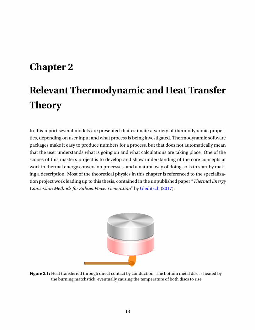
Figure 2.1: Heat transferred through direct contact by conduction. The bottom metal disc is heated bythe burning matchstick, eventually causing the temperature of both discs to rise.
13

CHAPTER 2. THEORY 14
2.1 Heat Transfer in General
The amount of thermal energy that is added to or removed from a system is what we call heat.
Heat can be defined as the energy that is transferred between systems, when they are at different
temperatures. It is common to label heat with the letter Q, and use the SI unit Joules. The flow of
heat changes the temperature of a system, but how much it is changed depends on two things.
The first thing it is dependent on is the systems mass; if the mass is increased more heat is
required to change its temperature. The second thing it is dependent on, is the specific heat
of the system. The specific heat is defined as a measure of how well a substance stores heat,
and every substance has its own value. When the specific heat of a substance is increased, it
means that more energy transfer in the form of heat is required to induce a temperature change.
Equation (2.1) defines heat for an in-compressible substance, and shows that the amount of
thermal energy transferred is equal to the mass multiplied with specific heat cp and temperature
change. A positive Q means that the energy is flowing into the system, and a negative prefix
would indicate that heat is flowing out. For gases it must be taken into account that pressure-
volume work in addition to heat transfer affects the internal energy of a substance, which can
be expressed by the first law of thermodynamics (Equation (2.2)). During a phase change the
internal energy of a substance will change even as its temperature is held fixed (∆T = 0). A
way to calculate how much heat is flowing in or out of a system during phase changes is to use
an entity called latent heat. Latent heat reflects the changes in internal energy during a phase
change, and in Equation (2.3) it is labelled with the letter L.
Q = m · cp ·∆T (2.1)
∆U =W +Q = P∆V +Q (2.2)
Q = m ·L (2.3)
Heat spreads in three different ways, by conduction, convection or by radiation. These occur
depending on the circumstances that are taking place, and several of these types of heat trans-
fer can happen simultaneously. In the remainder of this section conduction and convection will
be explained, as they are phenomena of great importance to the topics of this thesis.
Conduction is the heat transfer related to direct contact between atoms or molecules, where
kinetic energy is transferred as they vibrate. A good example of conduction would be when solid
metal discs are in contact with each other, here illustrated in Figure 2.1 where the bottom disc
is heated due to some source of energy. Because of direct contact between the discs, both discs
are expected to become of higher temperature. In metals the phenomenon of conduction is
especially prominent, because the atoms sit very neatly packed together and allows the kinetic

CHAPTER 2. THEORY 15
A
l
Figure 2.2: Cross-section and travel distance related to heat flow by conduction. If both discs are madeof the same metal, they possess the same κ.
energy to spread rapidly from one atom to the next. In thermodynamics, the letter κ is com-
monly used for thermal conductivity and represents how fast a material is at conducting heat.
Equation (2.4) shows how rate of heat transfer between two points by the means of conduction
can be calculated. In the equation, the letter A means cross sectional area, t is time and the
letter l is the distance between two points, see it illustrated in Figure 2.2.
Q
t= κ · A ·∆T
l(2.4)
Convection is another type of heat transfer mechanism, which has some similarities to conduc-
tion in the sense that it also is dependent on molecular contact. In conduction the molecules
collide because they are closely packed nearby each other, but in the case of convection they
tend to travel much greater spatial distances. The typical example of convection is when a tea
kettle is warmed on the stove. Since the kettle is warmed from below, the tea water at the bot-
tom will become warm first which causes the arrangement of molecules to expand to a lower
density and make them spread away from the heat source. As soon as the warm molecules have
moved, cooler molecules from higher up in the kettle will move downwards and take their place,
thus creating heat transfer in the kettle. Another example of convection is when hot fluids from
a reservoir below the ground come towards the surface through a production well, effectively
moving away from the heat source to a cooler environment. The basic relationship for heat
transfer by convection is given in Equation (2.5), where λ is the heat transfer coefficient, t is time
and As is the surface area of the substance. It should be noted that convection can be divided
into two types, forced convection and natural convection. Forced convection is heat transfer
that happens when a substance is forced into contact with another substance, like when a liquid
is forced to flow through a pipe. Natural convection happens naturally, for example when sea
water comes into contact with stationary subsea equipment. To perform calculations on con-
vection, one must rely on empirical Nusselt number-correlations to determine the heat transfer

CHAPTER 2. THEORY 16
coefficient λ. There are many different correlations to choose from depending on the situation,
and in Sections 2.3.5 and 3.5 of this thesis some are shown. For natural convection, the geome-
try of the contact surface becomes of importance and must be determined. If we are looking at
forced convection like flow through a pipe, one must determine the flow conditions possibly by
calculating the Reynolds number manually. If the convection happens naturally or forced under
laminar conditions, the heat transfer coefficient would be determined by the use of the Prandtl,
Grashof and Rayleigh numbers along with an empirical correlation fitting to the situation. The
Prandtl, Grashof and Rayleigh numbers are defined by Equations (2.6)-(2.8). If the convection
happens forced but under turbulent conditions, one would have to estimate the friction coeffi-
cient for the interface as well, and rely on a different correlation for λ.
Q
t=λ · As ·∆T (2.5)
Ra =Gr ·Pr (2.6)
Gr =g L3
g rβ∆T
ν2(2.7)
Pr = µcp
κ(2.8)
Nomenclature for Chapter 2.1
Q Heat (J)
m Mass (kg)
cp Specific heat (J/kg ·K)
∆T Temperature differential (K)
L Latent heat (J/kg)
t Time (s)
κ Thermal conductivity (W/m ·K)
A Cross-sectional area (m2)
∆U Change in internal energy (J)
W Pressure volume work (J)
l Distance (m)
λ Heat transfer coefficient (W/m2 ·K)
As Surface area (m2)
g Gravity (m/s2)
Lg r Flat plates: Vertical length (m)
Pipes: Diameter (m)
β Coefficient of thermal expansion (1/K)
ν Kinematic viscosity (m2/s)
µ Dynamic viscosity (Pa · s)

CHAPTER 2. THEORY 17
2.2 Potential Heat Energy in a Produced Hydrocarbon Mixture
In Section 3.1, an Aspen HYSYS routine that estimates the raw thermal power potential from a
fluid stream that is cooled is presented. The goal in that exercise is to see how much thermal
energy that has to transfer out of a fluid stream if the core temperature of the stream is reduced
by a set amount. This section will show why HYSYS is used for the numerical calculation with
an example that shows how difficult it is to solve accurately manually. Kindly find the nomen-
clature for the equations in the table at the end of the section.
The enthalpy H of a system is a measure of its internal energy U plus the product of its pres-
sure and volume, as defined by Equation (2.9). If we assume that a fluid has constant pressure,
an enthalpy change can be induced by heat, work or a volume change. If we make another as-
sumption that all the work done in the system is what the pressure does to change the volume,
then we end up with Equation (2.12) that shows that the change in enthalpy is effectively equal
to heat. When doing thermodynamic analysis often the letter h for specific enthalpy is used as
opposed to H . The specific enthalpy is defined as enthalpy divided by mass, and is convenient
because it changes the value into an intensive property, here given by Equation (2.13).
H =U +P ·V (2.9)
∆H =Q +W +∆(P ·V ) (2.10)
∆H =Q +−∆(P ·V )+∆(P ·V ) (2.11)
∆H =Q (2.12)
h = H
m(2.13)
Below are equations necessary to analytically express heat flow from a fluid stream that passes
through a cooler, as illustrated by Figure 2.3. Equations (2.14), (2.15) and (2.17) are derived from
the first law of thermodynamics, which states that the energy of an isolated system is constant.
The internal energy u and enthalpy h have here been expressed as intensive properties, there-
fore lower-case letters have been used.
∑Ei n =∑
Eout +∆Estor ag e (2.14)
W +mi n(ui n +Pi nVi n + v2i n
2+ g zi n) = Q +mout (uout +Pout Vout +
v2out
2+ g zout ) (2.15)
h = u +PV (2.16)

CHAPTER 2. THEORY 18
mi n(ui n +Pi nVi n + v2i n2 + g zi n) mout (uout +Pout Vout + v2
out2 + g zout )
Q W
Figure 2.3: Cooling process illustrated by a box that acts as control volume for energy conservationconsiderations.
W +mi n(hi n + v2i n
2+ g zi n) = Q +mout (hout +
v2out
2+ g zout ) (2.17)
Equation (2.17) shows that the difference in enthalpy between inlet and outlet streams of a
cooler can be used to calculate a value for heat. With constant rates, no work and no elevation
difference between the sides of the cooler, the terms for kinetic and potential energy will cancel
out and leave heat solely as a function of enthalpy difference. The enthalpy of a mixture of dif-
ferent fluids can then be expressed based on the mass fraction of each phase times its enthalpy.
The enthalpy of liquid (and solid) phase is equal to the product of cp and∆T , but the enthalpy of
gases is not as easily expressed. When we are dealing with a hydrocarbon mixture, the total heat
flux will be the sum of the contribution from each fluid, see Equation (2.18). Equation (2.19)
shows the expression for the total heat flux based on the mass fraction and enthalpy change of
each phase of a fluid stream consisting of water, oil and gas.
Q
t= Q = Qg +Qo +Qw (2.18)
Q = (mg∆hg +mo∆ho +mw∆hw ) (2.19)
To make numeric estimations by hand it is found convenient to write the mass flow rate in terms
of density and volumetric flow rate, as shown in Equation (2.20). Here the product of heat ca-
pacity and temperature difference has been substituted in for enthalpy change for the liquid
phase, but the same simplification can not be done for the gas.
Q = (mg∆hg +ρoVocp,o∆T +ρw Vw cp,w∆T ) (2.20)
There are multiple reasons that the simplifications done in the equations above could cause
large errors, and manual calculation of Equation (2.20) is never performed in this report be-
cause of these. In the previous section it was mentioned that if a substance was subject to phase
change, a property called latent heat is necessary to perform the calculation of heat and that

CHAPTER 2. THEORY 19
its temperature would remain unchanged during the transition. And as we now have seen, the
thermal potential of the hydrocarbon flow is a combination of multiple fluids in two different
phases. Further expressing the rate of heat transfer analytically quickly becomes very tedious,
as it must be taken into account that phase change may occur in one of the fluids while oth-
ers stay within their current phase. In theory, phase changes between hydrocarbons in gaseous
and liquid state could occur, thus keeping the temperature constant between them, whilst a
temperature drop indeed could take place for the water simultaneously. When it comes to the
energy calculation of heat from the gaseous phase, it also has to be taken into account that as
heat is transferred to the surroundings the gas will have a tendency to contract in volume, which
means the surroundings will do pressure-volume work on the system. Aspen HYSYS will be used
for further analysis as it is an extremely powerful tool that can predict thermodynamic proper-
ties based on equation of state, and makes it easier to detect enthalpy changes in a system and
get realistic estimates for the rate of heat transfer.
2.2.1 Early Evaluation of Tordis Raw Heat Potential
In Sections 4.1 and 4.2 the results from calculations on raw thermal heat potential from the
Tordis produced fluids are presented, where Aspen HYSYS was used to model the duty. This sec-
tion is included mainly to give the reader early understanding on the magnitude of the power
potential that is dealt with, which is done using relationships we have seen so far.
The heat source at Tordis is a fluid in mainly liquid state, which means Equation (2.21) can be
used to calculate an approximate of the heating potential. A more precise expression is given
in Equation (2.22) that requires knowledge of the enthalpy values of the wellstream at inlet and
outlet states, and can be used to calculate the potential accurately when a fraction of the well-
stream is in gaseous state. Table 2.1 contains the necessary data to calculate the raw thermal
heat potential of Tordis with the given conditions, here shown in Equation (2.23). The enthalpy
values were generated by flashing the brine and hydrocarbons at 75◦C and 20◦C in PVTsim and
among the data supplied by Equinor. As shown in the calculation, the Tordis raw thermal power
potential is approximately 46.5 MW.
Q = mCp∆T (2.21)
Q = m∆h (2.22)

CHAPTER 2. THEORY 20
Table 2.1: Mass rates and wellstream enthalpy values at possible cycle inlet and outlet conditions
Mass rate Enthalpy at 40 bara and 75◦C Enthalpy at 37 bara and 20◦C
Water 161 kg/s -2320.56 kj/kg -2585.4 kj/kgHC fluid 31.5 kg/s -176.44 kj/kg -299.86 kj/kg
Q = mw ater∆hw ater +mHC∆hHC
Q = mw ater (hw,i n −hw,out )+mHC (hHC ,i n −hHC ,out )
Q = 161 · (−2320.56−−2585.4)+31.5 · (−176.44−−299.86)
Q = 46.5 MW
(2.23)
Approximate Power Output Potential
Without going into the implications involving Tordis specifically, one can make an approxima-
tion for the net power output potential from ORC thermal heat conversion by multiplying the
raw power available with realistically achievable thermal efficiency factors. According to Het-
tiarachchi et al. (2007), possible cycle efficiency for power generation based on low tempera-
ture geothermal resources (in the 70-100◦C range) is approximately 5-10%. Equation (2.24) was
therefore calculated for cycle efficiency within the realistic range, in order to give an idea of the
plausible power output from Tordis thermal heat conversion. Realistic figures for net power
output for an ORC system at the field are seen to be between 2.33 MW and 4.65 MW. The energy
requirements for boosting at Tordis are approximately 4 MW, so a cycle with 9% or higher ther-
mal efficiency would cover a target output of this figure.
W = Q ×ηther mal (2.24)
Table 2.2: Tordis power output potential based on raw power availiable and cycle efficiencies from5-10%
Q 46.5 MW 46.5 MW 46.5 MW 46.5 MW 46.5 MW 46.5 MWηther mal 0.05 0.06 0.07 0.08 0.09 0.10
W 2.33 MW 2.79 MW 3.26 MW 3.72 MW 4.19 MW 4.65 MW

CHAPTER 2. THEORY 21
2.3 Binary Organic Rankine Cycle
In power plants all around the world geothermal resources are exploited by producing hot water
from the subsurface and using it as an energy source to generate power. Many of these facilities
are using an organic Rankine cycle for converting thermal energy into electricity, and to look at
how the geothermal plants are operating onshore would be a good idea before attempting any-
thing subsea. The plants that are using ORC can be further divided into two main groups; those
that are operating with a direct cycle and those that run a binary cycle. The binary cycle method
will be reviewed in detail in this chapter since it is directly relevant to the Tordis field which
produces mainly liquids, but both methods are highly relevant when it comes to hydrocarbon
thermal energy conversion in general. In fact, geothermal energy conversion companies deal
with limitations and challenges some of which are very similar to those of oil companies. As an
example of the similarities it is referred to DiPippo (2016) that lists the following five necessary
features that should be present in order to have a commercially viable geothermal resource.
• A large heat source
• Permeable reservoir
• Water supply
• Overlaying impervious rock
• A reliable recharge mechanism
As seen from the list, the hydrothermal reservoir characteristic requires many of the qualities
similar to what is expected of a hydrocarbon reservoir with the main difference being the com-
position of the hot fluid. The hot fluid can be referred to as the geothermal resource, and accord-
ing to Astolfi and Macchi (2017) the enthalpy is the most important parameter for geothermal
resource classification. The in-situ phase of the resource is also important when different de-
velopment options for the geothermal plants are considered. If dealing with mainly vapor it is
common to use direct expansion in a steam turbine for energy conversion, but if the water is
mainly liquid phase or 2-phases there is a range of binary configurations that needs to be con-
sidered. When thermal heat is converted to electricity with a binary subcritical cycle, that entails
having the hot fluid heat exchange with a secondary working fluid that has a low boiling point,
thus making the working fluid evaporate within a closed cycle. The evaporated working fluid is
then passed through a turbine to extract energy, before it is cooled back to liquid state by heat
exchanging with a coolant. As mentioned in the previous section, the binary cycle solution is
common when dealing with a geothermal resource that is in the in-situ state of liquid or a com-
bination of liquid and vapor, such as Tordis. But the specific configuration of the binary cycle
varies between power plants, so it is necessary to have a look on the design options and main
factors determining the design choice.

CHAPTER 2. THEORY 22
Astolfi and Macchi (2017) states that the thermodynamic analysis of a thermal fluid is based
mainly on the amount of non-condensable gases (NCG) and its enthalpy, which has to be con-
sidered in combination with the WH conditions to determine cycle configuration and an opti-
mal working fluid. A typical example of a NCG found in a geothermal resource is CO2, which
is not easily condensed by cooling unless the pressures are very high. Due to the detailed de-
scription by Astolfi and Macchi (2017), it acts as the main source of the theoretical information
contained further in this section, unless stated otherwise.
The main parameters affecting the binary cycle design are the following
• Enthalpy of the geothermal fluid at bottom hole conditions
• Amount of non-condensable gases
• Pressure at wellhead
• Phase at wellhead
• Fluid composition
• Size of the reservoir
The binary power plants are mainly characterized by what working fluids are in the cycles, what
cycle configurations are actually run, cooling media used and turbine technology applied. In
fact, there are five common binary cycle system configurations that can be used to extract heat
from resources in both gaseous and liquid phase. Three of these configurations are variations of
subcritical systems, and the other two are supercritical and combined cycles. The single pres-
sure level subcritical cycle (see Figure 2.5) is the least complex configuration of them all, and
will be of the main focus here due to its simplicity, it being very common in the industry and its
low amount of required parts.
The next few pages show how one would conduct thermodynamic analysis on such a cycle,
by going through each component and describing the flow of energy by equations. The main
goal is to give the reader an overview of how the binary cycle works, and what part the individ-
ual components play in the energy conversion system. This analysis begins with looking at the
material and energy flow through and from the turbine, and then moves clockwise through the
cycle as it is shown in Figure 2.5, and analysing every component in a similar manner.

CHAPTER 2. THEORY 23
P
h
Pump
Preheater
Evaporator
Turbine
CondenserIdealRealSat. curve
Figure 2.4: Pressure-enthalpy diagram of a subcritical binary thermal conversion process.
mw f , hw f −2
Ptur b
mw f , hw f −1
mw f , hw f −3
msw , hsw−1
msw , hsw−2
mw f , hw f −4
Ppump
mw f , hw f −5
mh f , hh f −1
mh f , hh f −2
mh f , hh f −3
Figure 2.5: Single pressure binary cycle with subcritical configuration.

CHAPTER 2. THEORY 24
2.3.1 Turbine Function and Analytic Thermodynamic Description
For an ORC application such as this it is necessary to have a turbine that can convert vapor
energy into mechanical energy that can do work. Three forms of energy associated with the va-
por are of interest, namely energy associated with kinetic movement, pressure and temperature.
The vapor enters the turbine through the main inlet valve from the evaporator. The turbine con-
sists of multiple sets of blades with alternating shapes. The odd number of bladerows counting
from the first set in axial direction are called rotors and can rotate, and even numbers are called
stators and are stationary. Figure 2.7 shows an industrial scale gas turbine. The rotor parts of the
turbine has airfoil shaped blades, that are located in spatially increasing sizes. The vapor energy
induces rotation onto the blades, because of lift force due to the pressure difference between
each side of every blade. After passing through a rotor, the velocity of the vapor is reduced.
Therefore, the stator that follows acts as a nozzle to increase vapor velocity and kinetic energy,
thus decreasing vapor pressure and temperature due to the laws of energy conservation. As
the reader may be well aware of, pressure is inversely proportional to volume when it comes to
gases which leads to a necessity of a volumetric expanding shape as pressure goes down since
the vapor will occupy more space. The reader is referred to Figure 2.4 to see conceptual turbine
pressure decrease effect on specific enthalpy. So, as the vapor moves through the multiple com-
partments it expands as it transfers energy onto the rotor blades, and each rotor stage has bigger
blades than the previous to ensure capture of more energy. The expanding shape also helps in
regard to the efficiency, because the gas expands as the pressure is reduced, and if the blade
length span was left unchanged the velocities would be too high and cause increased frictional
losses. Since the potential energy from a geothermal ORC system can not be considered con-
stant in time, but instead varies, it is smart to install a vapor flow governing mechanism before
the vapor inlet. This means that the rates into the turbine can be regulated, keeping the rotor
rpm close to constant. As a matter of fact, the frequency of electric power produced is directly
proportional to the generator speed. Once the vapor has passed through all stages, it can be
exhausted into the condenser for regeneration.
When it comes to turbine (and pump) engineering, an entity called the isentropic efficiency is
often used to convert from ideal to real conditions. It is defined as the ratio between real work
and isentropic work, and is given by Equation (2.25). The turbine power can be expressed as
by Equation (2.26), but note that this value represents mechanical power and needs to be con-
verted to grid power by multiplication by generator efficiency. When performing calculations,
one must be careful to consider the real turbine operating conditions, specifically making a note
of the working fluid phase. Even though the fluid has undergone preheating and evaporation
processes before passing through the turbine, it is possible that it retains some liquid in form of
droplets. The presence of liquid has a negative effect on the turbine efficiency, and also leads to

CHAPTER 2. THEORY 25
increased wear of the physical equipment. According to Baumann (1921) it is relatively simple
to take the presence of moisture into account when calculating turbine efficiency. His rule is
still considered as valid, and it states that one percent moisture leads to one percent lower tur-
bine efficiency, in general. The rule was given by Equation (2.27) as a function of wetness yw f ,
but can easily be expressed as a function of dryness by multiplication of the dry isentropic effi-
ciency value with average dryness of the working fluid xw f . The constant a can vary, but in most
cases it can safely be assumed equal to one. That gives Equations (2.28) and (2.29). In Figure 2.6
blue arrows represents the material streams composed of the working fluid, while the red arrow
represents turbine energy output.
mw f , hw f −2
Ptur b
mw f , hw f −1
Figure 2.6: Simple sketch of a turbine.
ηtur b = hw f −1 −hw f −2
hw f −1 −h2,i deal(2.25)
Ptur b = mw f (hw f −1 −hw f −2) = mw f ηtur b(hw f −1 −h2,i deal ) (2.26)
ηtur b,wet = ηtur b · (1−a · yw f −1 + yw f −2
2) (2.27)
ηtur b,wet = ηtur b · (1− yw f −1 + yw f −2
2) (2.28)
ηtur b,wet = ηtur b ·xw f −1 +xw f −2
2(2.29)

CHAPTER 2. THEORY 26
Figure 2.7: Siemens SGT-400, 14.3 MW industrial gas turbine. Photo taken from Siemens.com
Figure 2.8: Amarinth U Series industrial centrifugal pump, rated for 10 bar. Photo taken fromamarinth.com

CHAPTER 2. THEORY 27
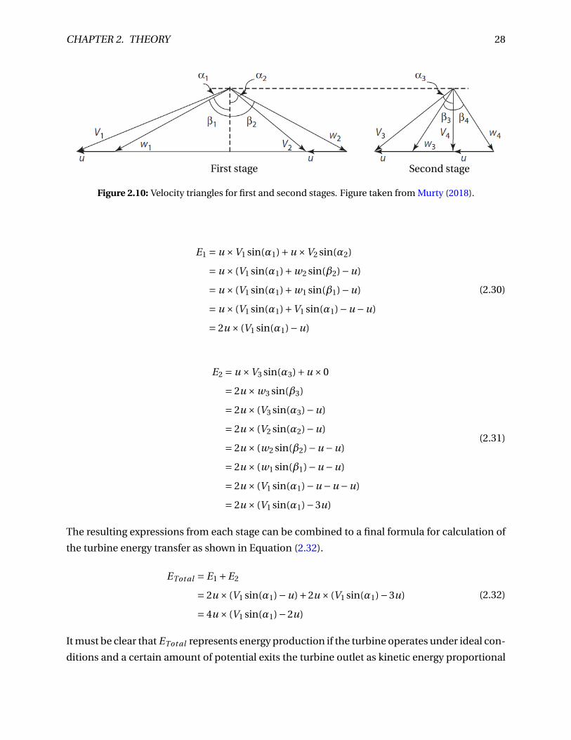
Figure 2.9: Turbine pressure and velocity profiles shown for initial two stages. Figure taken from Murty(2018).
Velocity Compounding in Turbine Design
The ORC turbine must be designed such that the required energy transfer can be achieved by
having a sufficiently high isentropic efficiency factor. Velocity compounding is an alternative
design method commonly used in modern turbines to obtain high enthalpy drop and reason-
able rotor tip speeds, by compounding the energy generation process into multiple smaller
stages. An illustration of the method is shown in Figure 2.9 and it can be seen how the entire
pressure drop happens when the gas passes through the nozzle, then flow velocity is decreased
with every rotor row until the kinetic energy becomes negligible at the final stage (Murty (2018)).
The physical setup guides the working fluid through the stages after the nozzle without making
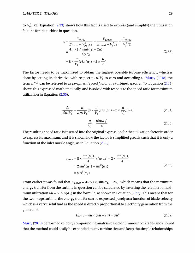
impact on the pressure state, and the corresponding velocity diagrams are shown in Figure 2.10.
These diagrams are very useful because equations can be derived for calculation of the energy
transfer related to each stage based on the changes in fluid velocity. Equation (2.30) shows how
the energy transfer of the first stage E1 can be simplified to an expression which is only based on
blade velocity u, absolute fluid velocity V and nozzle inlet angle α1. A similar derivation can be
done for the second stage, here shown in Equation (2.31). For following the derivation, it should
be noted that the following relationships holds true; relative velocities w1 = w2 and w3 = w4,
blade angles β1 =β2 and β3 =β4, fluid velocities V2 =V3 and nozzle angles α2 =α3.
CHAPTER 2. THEORY 28
First stage Second stage
Figure 2.10: Velocity triangles for first and second stages. Figure taken from Murty (2018).
E1 = u ×V1 sin(α1)+u ×V2 sin(α2)
= u × (V1 sin(α1)+w2 sin(β2)−u)
= u × (V1 sin(α1)+w1 sin(β1)−u)
= u × (V1 sin(α1)+V1 sin(α1)−u −u)
= 2u × (V1 sin(α1)−u)
(2.30)
E2 = u ×V3 sin(α3)+u ×0
= 2u ×w3 sin(β3)
= 2u × (V3 sin(α3)−u)
= 2u × (V2 sin(α2)−u)
= 2u × (w2 sin(β2)−u −u)
= 2u × (w1 sin(β1)−u −u)
= 2u × (V1 sin(α1)−u −u −u)
= 2u × (V1 sin(α1)−3u)
(2.31)
The resulting expressions from each stage can be combined to a final formula for calculation of
the turbine energy transfer as shown in Equation (2.32).
ETot al = E1 +E2
= 2u × (V1 sin(α1)−u)+2u × (V1 sin(α1)−3u)
= 4u × (V1 sin(α1)−2u)
(2.32)
It must be clear that ETot al represents energy production if the turbine operates under ideal con-
ditions and a certain amount of potential exits the turbine outlet as kinetic energy proportional
CHAPTER 2. THEORY 29
to V 2out /2. Equation (2.33) shows how this fact is used to express (and simplify) the utilization
factor ε for the turbine in question.
ε= Etot al
Etot al +V 2out /2
= Etot al
Etot al +V 24 /2
= Etot al
V 21 /2
= 4u × (V1 sin(α1)−2u)
V 21 /2
= 8× u
V1(si n(α1)−2× u
V1)
(2.33)
The factor needs to be maximized to obtain the highest possible turbine efficiency, which is
done by setting its derivative with respect to u/V1 to zero and according to Murty (2018) the
term u/V1 can be referred to as peripheral speed factor or a turbine’s speed ratio. Equation (2.34)
shows this expressed mathematically, and is solved with respect to the speed ratio for maximum
utilization in Equation (2.35).
dε
du/V1= d
du/V1[8× u
V1(si n(α1)−2× u
V1)] = 0 (2.34)
u
V1= sin(α1)
4(2.35)
The resulting speed ratio is inserted into the original expression for the utilization factor in order
to express its maximum, and it is shown how the factor is simplified greatly such that it is only a
function of the inlet nozzle angle, as in Equation (2.36).
εmax = 8× sin(α1)
4(si n(α1)−2× sin(α1)
4)
= 2sin2(α1)− sin2(α1)
= sin2(α1)
(2.36)
From earlier it was found that ETot al = 4u × (V1 sin(α1)−2u), which means that the maximum
energy transfer from the turbine in question can be calculated by inserting the relation of maxi-
mum utilization 4u =V1 sin(α1) in the formula, as shown in Equation (2.37). This means that for
the two-stage turbine, the energy transfer can be expressed purely as a function of blade velocity
which is a very useful find as the speed is directly proportional to electricity generation from the
generator.
EM ax = 4u × (4u −2u) = 8u2 (2.37)
Murty (2018) performed velocity compounding analysis based on n amount of stages and showed
that the method could easily be expanded to any turbine size and keep the simple relationships
CHAPTER 2. THEORY 30
for energy transfer calculation that was found for two stages, and the formulas are given here
by Equation (2.38) and Equation (2.39). With the turbine energy transfer being proportional to
the number of stages squared, it is clear that every added stage gives a significant benefit to its
overall efficiency.
En = 2n2u2 (2.38)
u
V1= sin(α1)
2n(2.39)
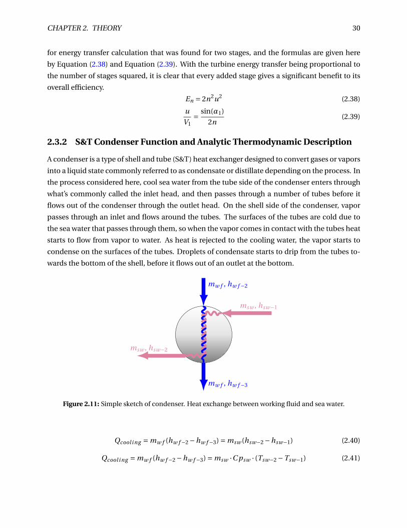
2.3.2 S&T Condenser Function and Analytic Thermodynamic Description
A condenser is a type of shell and tube (S&T) heat exchanger designed to convert gases or vapors
into a liquid state commonly referred to as condensate or distillate depending on the process. In
the process considered here, cool sea water from the tube side of the condenser enters through
what’s commonly called the inlet head, and then passes through a number of tubes before it
flows out of the condenser through the outlet head. On the shell side of the condenser, vapor
passes through an inlet and flows around the tubes. The surfaces of the tubes are cold due to
the sea water that passes through them, so when the vapor comes in contact with the tubes heat
starts to flow from vapor to water. As heat is rejected to the cooling water, the vapor starts to
condense on the surfaces of the tubes. Droplets of condensate starts to drip from the tubes to-
wards the bottom of the shell, before it flows out of an outlet at the bottom.
mw f , hw f −2
mw f , hw f −3
msw , hsw−1
msw , hsw−2
Figure 2.11: Simple sketch of condenser. Heat exchange between working fluid and sea water.
Qcool i ng = mw f (hw f −2 −hw f −3) = msw (hsw−2 −hsw−1) (2.40)
Qcool i ng = mw f (hw f −2 −hw f −3) = msw ·C psw · (Tsw−2 −Tsw−1) (2.41)
CHAPTER 2. THEORY 31
A good illustration of a shell and tube heat exchanger is given in Figure 2.21. It is worth men-
tioning that as the vapor condenses a low pressure is created inside the condenser, which means
that the engineer must make sure the vapor entry pressure is sufficiently high at all times to en-
sure inflow. Since the heat that leaves the hot vapor is equal in amount to the heat received to
the cool water, the rate of heat transfer can be expressed as in Equation (2.40). If we consider a
case where the specific heat capacity of the sea water is not changing, the heat flow can be ex-
pressed in terms of the corresponding temperature increase which is easily measured, as shown
in Equation (2.41). The working fluid material stream is illustrated in blue color as in previous
figures, and the sea water material stream is shown in pink in Figure 2.11.
Condensation
When the organic Rankine cycle is designed based on using a working fluid operating on a sub-
critical pressure condition it means that phase change of the fluid will occur in the heating and
cooling systems. To calculate realistic values for the heat transfer coefficients when the work-
ing fluid condenses or evaporates one needs to use some additional empirical correlations to
accommodate the latent heat involved in these processes. The Kern equations for heat transfer
coefficient to be used for condensation processes are shown below. For an ORC with access to
cooling brine the heat sink is to be considered isothermal and Equation (2.42) is used for gravi-
tation driven isothermal condensation. The value for G in the Kern method is dependent on the
condenser geometric configuration of which there are four main choices, horizontal tubes, hor-
izontal tube bundle, vertical tubes and vertical tube bundle which are shown in their respective
order in Equations (2.43)-(2.46). If the condensation is vertical under turbulent and wavy flow,
the correction factor ftc defined in Equation (2.47) is multiplied with the initial heat transfer co-
efficient as seen in Equation (2.48). If vertical condensation happens under conditions of very
high turbulence, Kern proposes Equation (2.49) for the heat transfer coefficient.
αg =0.925κρ2g
ηG(2.42)
Gt s,H = Ml i qui d
1800nπltube(2.43)
Gss,H = Ml i qui d
3600n0.66ltube(2.44)
Gt s,V = Ml i qui d
3600nπDi(2.45)
Gss,V = Ml i qui d
3600nπDo(2.46)
ftc = 0.8(Re
4)0.11 = 0.8(
GV
η)0.11, 40 < Re (2.47)

CHAPTER 2. THEORY 32
αw = ftcαg (2.48)
αt = 0.0076(κ3ρ2g
η2)1/3 × (
4GV
η)0.4, 2100 < Re (2.49)
Nomenclature for the Kern equations
List of variables:
αg Heat transfer coeff. for grav.-driven
isothermal cond. (W/m2 ·k)
κ Thermal conductivity (W/m ·K)
g Gravity (m/s2)
ρ Density (kg/m3)
η Dynamic viscosity (Pa · s)
Ml i qui d Mass rate (kg/h)
n Number of tubes (−)
ltube Tube length (m)
Di Inner diameter (m)
Do Outer diameter (m)
ftc Turbulence correction factor (−)
Re Reynolds number (−)
αw Corrected heat transfer coeff. (W/m2 ·k)
αt High turb. flow heat transfer coeff.
(W/m2 ·k)
2.3.3 Other Types of Subsea Cooling Equipment
A traditional flow assurance challenge has been to maintain a certain level of temperature in
the flow lines in order to ensure that problems related to things like wax, asphaltenes and hy-
drates do not occur. But sometimes an opposite problem needs solving for optimum field de-
velopment, the problem of cooling the wellstream subsea to accommodate a certain need. An
example situation is when compression subsea is performed and subsea cooling is required to
counteract the corresponding temperature rise, or when very high temperature crude is cooled
to the point where less expensive piping is applicable due to less corrosion. Because of chal-
lenges such as these, a number of subsea cooling systems have been developed by oil service
companies in the later years. In this section an overview of some of these systems and their
main principles are shown, since the systems potentially could be applied in subsea organic
Rankine cycles in place of a regular condenser.
In the SPE published paper Subsea Cooling; Passive, Active or Sea Current Controlled? Rudh
et al. (2016) has listed passive manifold coolers, sectioned passive coolers, by-pass coolers, sea
current controlled coolers and shell and tube coolers as the main cooling technologies to be
used subsea. Shell and tube coolers are not reviewed in this section due to having been intro-
duced earlier in this thesis and neither is sea current controlled coolers because of not yet being
commercially available.

CHAPTER 2. THEORY 33
Figure 2.12: Passive Manifold Cooler principle illustration. Fluid enters the coils from main pipeline andsea water cools it down by means of natural convection.
Passive Manifold Cooler
A passive manifold cooler is illustrated in Figure 2.12. It is based on splitting the main flow line
into numerous smaller less isolated tubes that are coiled in parallel. A high degree of natural
convection will occur to cool the medium inside the coils while requiring no powering of the
apparatus. The main reason behind splitting the stream into multiple channels is to deal with
potential multi-phase flow, and when the passive cooler is applied in a traditional manner one
needs to be aware that the temperature distribution will not be completely even between the
different coils. This means that certain local temperature minimums may cause flow assurance
issues, but this would be less of a concern when the unit is run in a ORC since no deposits are to
be expected from the working fluid. According to Rudh et al. (2016) the size of the coils used are
usually between 1 and 2 inches and usually made of super duplex stainless steel with no coating.
Figure 2.13 show a passive manifold cooler that is developed by Future Technology AS.
Figure 2.13: A Future Technology AS passive subsea cooler. Cools up to 50 MW and can be scaled tocustomer needs. Image taken from http://futuretechnology.no/fscc/.

CHAPTER 2. THEORY 34
Figure 2.14: Principle illustration of a sectioned passive manifold cooler. Operator can control thecooling duty by routing the working fluid through the chosen coils based on need.
Figure 2.15: A Future Technology AS 5-100% controllable subsea cooler. Cools up to 50 MW and can bescaled to customer needs. Image taken from http://futuretechnology.no/fscc/.

CHAPTER 2. THEORY 35
Figure 2.16: Principle illustration of a by-pass cooler. Outlet temperature can be controlled with highaccuracy using the choke.
Sectioned Passive Cooler
Figure 2.14 shows the principle behind the sectioned passive cooling manifold, red colored ar-
rows here represents a fluid of original temperature and blue arrows represents the cooled fluid
that leaves the heat exchanger. As seen from the illustration, a setup like this allows for some
control of the condition of the outlet fluid. The isolation valves can be operated by ROV or simi-
lar to adjust the area of heat transfer and hence the heat duty of the cooler. Since having accurate
cooling duty is very important for any thermodynamic cycle, using a sectioned cooler would be
preferable as compared to basic passive cooling. Future Technology AS developed the FSCC -
Future Subsea Controllable Cooler that is shown in Figure 2.15, and it is suited to transfer up to
50 MW worth of thermal energy.
By-pass Cooler
Figure 2.16 illustrates the concept of the by-pass cooler. Rudh et al. (2016) states that even
though this setup allows the temperature to be controlled with very high accuracy, there are po-
tential problems if operation is under high turn-down and most of the fluid is directed through
the choke. This is because the minor fraction of fluid that actually passes through the cooling
system will be very cold and can pose a flow assurance challenge.
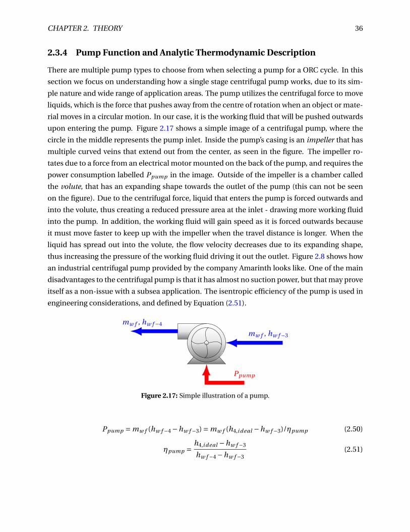
CHAPTER 2. THEORY 36
2.3.4 Pump Function and Analytic Thermodynamic Description
There are multiple pump types to choose from when selecting a pump for a ORC cycle. In this
section we focus on understanding how a single stage centrifugal pump works, due to its sim-
ple nature and wide range of application areas. The pump utilizes the centrifugal force to move
liquids, which is the force that pushes away from the centre of rotation when an object or mate-
rial moves in a circular motion. In our case, it is the working fluid that will be pushed outwards
upon entering the pump. Figure 2.17 shows a simple image of a centrifugal pump, where the
circle in the middle represents the pump inlet. Inside the pump’s casing is an impeller that has
multiple curved veins that extend out from the center, as seen in the figure. The impeller ro-
tates due to a force from an electrical motor mounted on the back of the pump, and requires the
power consumption labelled Ppump in the image. Outside of the impeller is a chamber called
the volute, that has an expanding shape towards the outlet of the pump (this can not be seen
on the figure). Due to the centrifugal force, liquid that enters the pump is forced outwards and
into the volute, thus creating a reduced pressure area at the inlet - drawing more working fluid
into the pump. In addition, the working fluid will gain speed as it is forced outwards because
it must move faster to keep up with the impeller when the travel distance is longer. When the
liquid has spread out into the volute, the flow velocity decreases due to its expanding shape,
thus increasing the pressure of the working fluid driving it out the outlet. Figure 2.8 shows how
an industrial centrifugal pump provided by the company Amarinth looks like. One of the main
disadvantages to the centrifugal pump is that it has almost no suction power, but that may prove
itself as a non-issue with a subsea application. The isentropic efficiency of the pump is used in
engineering considerations, and defined by Equation (2.51).
mw f , hw f −4
mw f , hw f −3
Ppump
Figure 2.17: Simple illustration of a pump.
Ppump = mw f (hw f −4 −hw f −3) = mw f (h4,i deal −hw f −3)/ηpump (2.50)
ηpump = h4,i deal −hw f −3
hw f −4 −hw f −3(2.51)
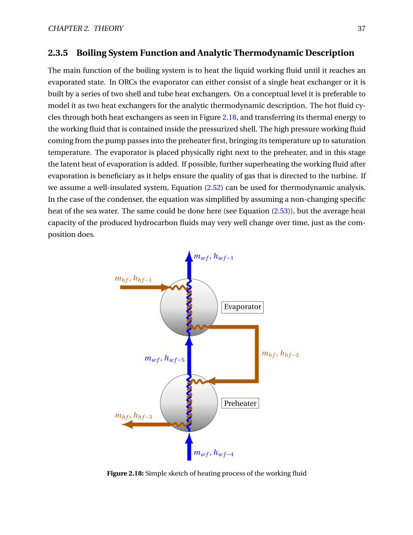
CHAPTER 2. THEORY 37
2.3.5 Boiling System Function and Analytic Thermodynamic Description
The main function of the boiling system is to heat the liquid working fluid until it reaches an
evaporated state. In ORCs the evaporator can either consist of a single heat exchanger or it is
built by a series of two shell and tube heat exchangers. On a conceptual level it is preferable to
model it as two heat exchangers for the analytic thermodynamic description. The hot fluid cy-
cles through both heat exchangers as seen in Figure 2.18, and transferring its thermal energy to
the working fluid that is contained inside the pressurized shell. The high pressure working fluid
coming from the pump passes into the preheater first, bringing its temperature up to saturation
temperature. The evaporator is placed physically right next to the preheater, and in this stage
the latent heat of evaporation is added. If possible, further superheating the working fluid after
evaporation is beneficiary as it helps ensure the quality of gas that is directed to the turbine. If
we assume a well-insulated system, Equation (2.52) can be used for thermodynamic analysis.
In the case of the condenser, the equation was simplified by assuming a non-changing specific
heat of the sea water. The same could be done here (see Equation (2.53)), but the average heat
capacity of the produced hydrocarbon fluids may very well change over time, just as the com-
position does.
mw f , hw f −1
mw f , hw f −5
mh f , hh f −1
mh f , hh f −2
mw f , hw f −4
mh f , hh f −3
Evaporator
Preheater
Figure 2.18: Simple sketch of heating process of the working fluid
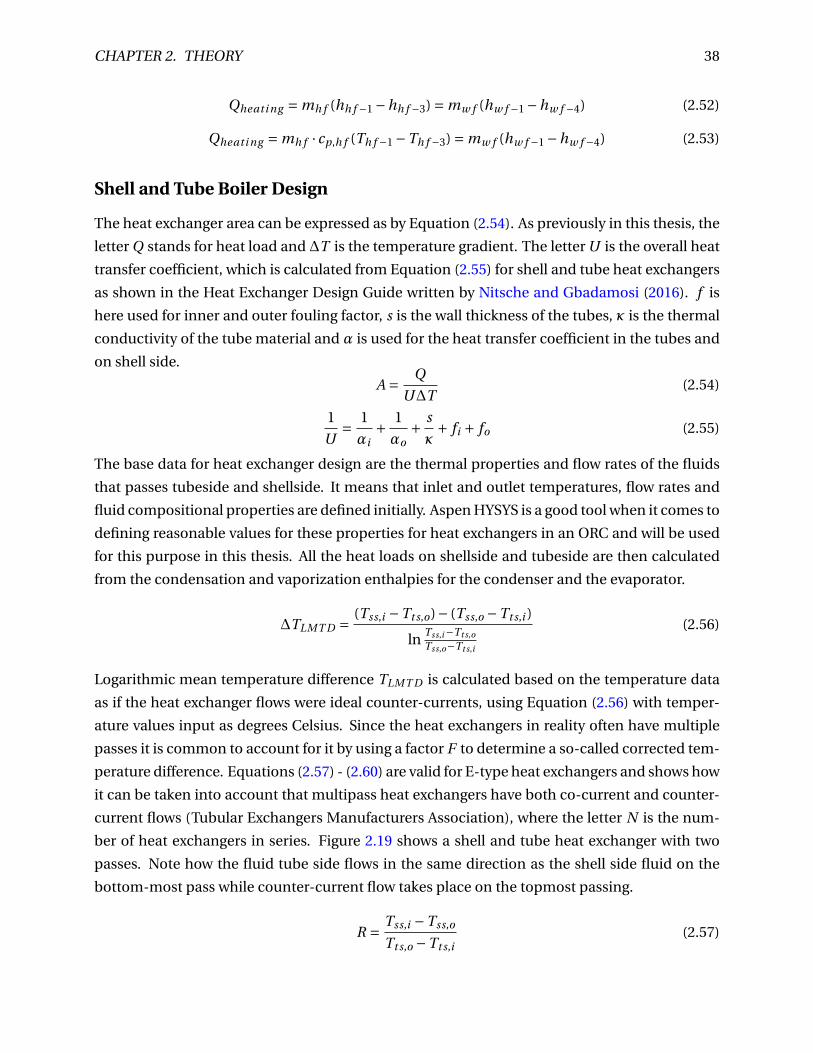
CHAPTER 2. THEORY 38
Qheati ng = mh f (hh f −1 −hh f −3) = mw f (hw f −1 −hw f −4) (2.52)
Qheati ng = mh f · cp,h f (Th f −1 −Th f −3) = mw f (hw f −1 −hw f −4) (2.53)
Shell and Tube Boiler Design
The heat exchanger area can be expressed as by Equation (2.54). As previously in this thesis, the
letter Q stands for heat load and ∆T is the temperature gradient. The letter U is the overall heat
transfer coefficient, which is calculated from Equation (2.55) for shell and tube heat exchangers
as shown in the Heat Exchanger Design Guide written by Nitsche and Gbadamosi (2016). f is
here used for inner and outer fouling factor, s is the wall thickness of the tubes, κ is the thermal
conductivity of the tube material and α is used for the heat transfer coefficient in the tubes and
on shell side.
A = Q
U∆T(2.54)
1
U= 1
αi+ 1
αo+ s
κ+ fi + fo (2.55)
The base data for heat exchanger design are the thermal properties and flow rates of the fluids
that passes tubeside and shellside. It means that inlet and outlet temperatures, flow rates and
fluid compositional properties are defined initially. Aspen HYSYS is a good tool when it comes to
defining reasonable values for these properties for heat exchangers in an ORC and will be used
for this purpose in this thesis. All the heat loads on shellside and tubeside are then calculated
from the condensation and vaporization enthalpies for the condenser and the evaporator.
∆TLMT D = (Tss,i −Tt s,o)− (Tss,o −Tt s,i )
lnTss,i−Tt s,o
Tss,o−Tt s,i
(2.56)
Logarithmic mean temperature difference TLMT D is calculated based on the temperature data
as if the heat exchanger flows were ideal counter-currents, using Equation (2.56) with temper-
ature values input as degrees Celsius. Since the heat exchangers in reality often have multiple
passes it is common to account for it by using a factor F to determine a so-called corrected tem-
perature difference. Equations (2.57) - (2.60) are valid for E-type heat exchangers and shows how
it can be taken into account that multipass heat exchangers have both co-current and counter-
current flows (Tubular Exchangers Manufacturers Association), where the letter N is the num-
ber of heat exchangers in series. Figure 2.19 shows a shell and tube heat exchanger with two
passes. Note how the fluid tube side flows in the same direction as the shell side fluid on the
bottom-most pass while counter-current flow takes place on the topmost passing.
R = Tss,i −Tss,o
Tt s,o −Tt s,i(2.57)

CHAPTER 2. THEORY 39
P = Tt s,o −Tt s,i
Tss,i −Tt s,i(2.58)
Pz =1− ( RP−1
P−1 )1/N
R − ( RP−1P−1 )1/N
(2.59)
F =p
R2 +1
R −1
ln[(1−Pz)/(1−RPz)]
ln[ (2/Pz )−1−R+p
R2+1
(2/Pz )−1−R−p
R2+1]
(2.60)
Nitsche and Gbadamosi (2016) states that the temperature efficiency factor F should always be
higher than 0.75 and it is simply multiplied with the logarithmic mean temperature difference to
get a more realistic gradient, as shown in Equation (2.61). ∆TC MT D can then be substituted into
Equation (2.54) for calculation of the heat exchanger surface area based on assumed value for
U . Once the required area is found one needs a data table like the one shown in Table 2.3 which
is used to select a heat exchanger with sufficient size and volume flow rates. Once a specific
configuration has been selected one calculates the real flow velocities in tubes and the shell,
and use the result to determine the Reynolds number for the flow with Equation (2.62).
∆TC MT D = F∆TLMT D (2.61)
Re = v ×D
ν(2.62)
Pr = 3600νC pρ
κ(2.63)
The heat transfer coefficients αt s and αss for the tube- and shellside has to be determined, and
as seen by Equations (2.69)-(2.70), it can be defined by the Nusselt number Nu, the pipe di-
ameter D and the thermal conductivity of the fluid κ. A value for the diameter can be selected
based on the heat exchanger under consideration, and finding the thermal conductivity of the
hot fluid mixture can be done with the thermodynamic modeling software. The Nusselt number
has to be calculated with empirical correlations, and there exists a number of Nu-correlations
valid for a range of different applications. The definitions given by Equation (2.64), (2.65) and
(2.66) are suitable for tube side heat transfer according to the Nitsche method and Equations
(2.67) - (2.68) can be used for calculations shellside. The heat transfer coefficient for tubeside
should always be converted to outer tube diameter because heat exchangers are specified based
on outer area, and such conversion is easily done by multiplication with the fraction of inner to
outer diameter, as shown in Equation (2.71).
Nut s = 1.86Re ×Pr ×D
l, Re < 2300 (2.64)

CHAPTER 2. THEORY 40
Table 2.3: Geometric data of heat exchangers according to DIN 28,184, part 1, for 25 × 2 tubes with 32mm triangular pitch. Data taken from Nitsche and Gbadamosi (2016).
Type DN Z Da B n AE AR AS fw VR VMnr. [-] [-] [mm] [mm] [-] [mm2] [mm2] [m2/m] [-] [m3/h] [m3/h]
1 150 2 168 30 14 1770 2425 1.1 0.251 8.73 6.372 200 2 219 40 26 2288 4503 2 0.366 16.21 8.243 250 2 273 50 44 5520 7620 3.5 0.259 27.43 19.874 300 2 324 60 66 5088 11,430 5.2 0.375 41.15 18.325 350 2 355 70 76 6230 13,162 6 0.397 47.38 22.436 350 4 355 70 68 6230 5888 5.3 0.381 21.20 22.437 400 2 406 80 106 11,072 18,357 8.3 0.319 66.09 39.868 400 4 406 80 88 9072 7620 6.9 0.382 27.43 32.669 500 2 508 100 180 14,600 31,172 14.1 0.360 112.22 52.5610 500 4 508 100 164 12,100 14,201 12.9 0.430 51.12 43.5611 600 2 600 120 258 19,560 44,681 20.3 0.389 160.85 70.4212 600 8 600 120 232 22,560 10,044 18.2 0.348 36.16 81.2213 700 2 700 140 364 22,260 63,038 28.6 0.456 226.94 80.1414 700 8 700 140 324 25,760 14,028 25.4 0.395 50.50 92.7415 800 2 800 160 484 29,440 83,819 38 0.454 301.75 105.9816 800 8 800 160 432 37,440 18,703 33.9 0.367 67.33 134.7817 900 2 900 180 622 41,400 107,718 48.9 0.407 387.79 149.0418 900 8 900 180 556 41,400 24,072 43.7 0.416 86.66 149.0419 1000 2 1000 200 776 46,000 134,388 61 0.452 483.80 165.6020 1000 8 1000 200 712 56,000 30,826 55.9 0.373 110.97 201.6021 1100 2 1100 220 934 55,220 161,750 73.4 0.460 582.30 198.7922 1100 8 1100 220 860 60,720 37,234 67.5 0.420 134.05 218.5923 1200 2 1200 240 1124 72,240 194,655 88.3 0.416 700.76 260.0624 1200 8 1200 240 1048 78,240 45,373 82.3 0.390 163.34 281.66
DN = Nominal shell diameter; Z = number of tube passes; Da = shell diameter [mm]; B = baffle spacing[mm]; n = number of tubes; AE = shell-side flow cross section [mm2]; AR = tube-side flow cross section[mm2]; AS = Heat exchanger area per m tube length [m2/m]; VR = Required flow rate for 1 m/s flowvelocity on the tube side [m3/h]; VM = Required flow rate for 1 m/s flow velocity at the shell side [m3/h].
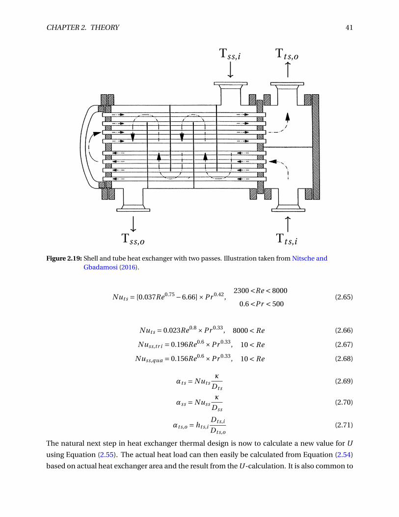
CHAPTER 2. THEORY 41
Tss,i Tt s,o
Tt s,iTss,o
Figure 2.19: Shell and tube heat exchanger with two passes. Illustration taken from Nitsche andGbadamosi (2016).
Nut s = [0.037Re0.75 −6.66]×Pr 0.42,2300 <Re < 8000
0.6 <Pr < 500(2.65)
Nut s = 0.023Re0.8 ×Pr 0.33, 8000 < Re (2.66)
Nuss,tr i = 0.196Re0.6 ×Pr 0.33, 10 < Re (2.67)
Nuss,qua = 0.156Re0.6 ×Pr 0.33, 10 < Re (2.68)
αt s = Nut sκ
D t s(2.69)
αss = Nussκ
Dss(2.70)
αt s,o = ht s,iD t s,i
D t s,o(2.71)
The natural next step in heat exchanger thermal design is now to calculate a new value for U
using Equation (2.55). The actual heat load can then easily be calculated from Equation (2.54)
based on actual heat exchanger area and the result from the U -calculation. It is also common to

CHAPTER 2. THEORY 42
see how much area your selected configuration has to spare and also check the excess fouling.
These values can be estimated by application of Equation (2.72) and Equation (2.73).
Aexcess,[%] = (100Uactual
Ur equi r ed)−100 (2.72)
fexcess,[m2K /W ] =Uactual −Ur equi r ed
Uactual ×Ur equi r ed(2.73)
2.3.6 Exchanger Tube Patterns and Baffles
The engineers need to make some decisions of the geometry of the unit before the thermal per-
formance of a shell and tube heat exchanger design can be estimated. The most important ge-
ometric consideration is deciding on what tube pattern will be used in the exchanger, a choice
that has direct influence on the temperature profile which will be achieved. Performance-wise,
using a triangular pattern as seen in Figure 2.20a is very good since the fluid shell side is forced
"onto" the tubes when it flows towards the shell-side outlet. This means that the heat transfer
coefficient when using a triangular pattern is higher than when a square pattern is used. Figure
2.20b shows how flow through a shell with tubing in a square pattern does not force the work-
ing fluid onto the tubes in the same way, hence performing worse. The positive side of using a
square pattern is that it is much easier to clean, so in cases where deposits of wax, asphaltene
or similar will occur then using square pattern tubing is convenient. It should be noted that
in a ORC the working fluid is always run shell-side, so these types of flow assurance issues are
not present except possibly inside the tubes where the heat source flows. In cases where square
pattern has to be used in the exchanger, it is often opted to rotate the squares as seen in Figure
2.20c to improve the heat transfer coefficient.
(a) Triangular tube pattern. (b) Square tube pattern. (c) Rotated square tube pattern.
Figure 2.20: Overview of common tube patterns geometry. Red arrow represents flow direction fromshell-side inlet at the bottom towards shell-side outlet at the top.
A baffle is another physical object installed on the shell side of the S&T exchanger and it func-
tions as an obstacle to the flow of the working fluid, effectively forcing it into a certain direction.
In practice multiple baffles are usually installed, thus creating a sinusoidal flow pattern as seen
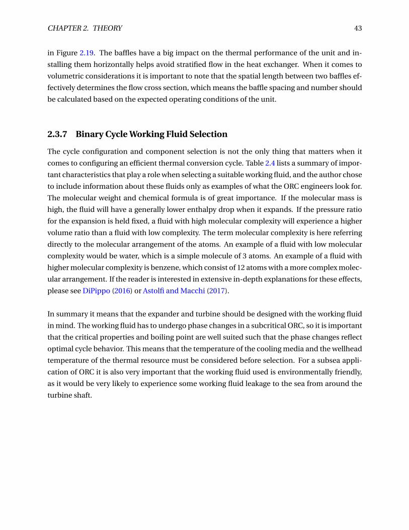
CHAPTER 2. THEORY 43
in Figure 2.19. The baffles have a big impact on the thermal performance of the unit and in-
stalling them horizontally helps avoid stratified flow in the heat exchanger. When it comes to
volumetric considerations it is important to note that the spatial length between two baffles ef-
fectively determines the flow cross section, which means the baffle spacing and number should
be calculated based on the expected operating conditions of the unit.
2.3.7 Binary Cycle Working Fluid Selection
The cycle configuration and component selection is not the only thing that matters when it
comes to configuring an efficient thermal conversion cycle. Table 2.4 lists a summary of impor-
tant characteristics that play a role when selecting a suitable working fluid, and the author chose
to include information about these fluids only as examples of what the ORC engineers look for.
The molecular weight and chemical formula is of great importance. If the molecular mass is
high, the fluid will have a generally lower enthalpy drop when it expands. If the pressure ratio
for the expansion is held fixed, a fluid with high molecular complexity will experience a higher
volume ratio than a fluid with low complexity. The term molecular complexity is here referring
directly to the molecular arrangement of the atoms. An example of a fluid with low molecular
complexity would be water, which is a simple molecule of 3 atoms. An example of a fluid with
higher molecular complexity is benzene, which consist of 12 atoms with a more complex molec-
ular arrangement. If the reader is interested in extensive in-depth explanations for these effects,
please see DiPippo (2016) or Astolfi and Macchi (2017).
In summary it means that the expander and turbine should be designed with the working fluid
in mind. The working fluid has to undergo phase changes in a subcritical ORC, so it is important
that the critical properties and boiling point are well suited such that the phase changes reflect
optimal cycle behavior. This means that the temperature of the cooling media and the wellhead
temperature of the thermal resource must be considered before selection. For a subsea appli-
cation of ORC it is also very important that the working fluid used is environmentally friendly,
as it would be very likely to experience some working fluid leakage to the sea from around the
turbine shaft.
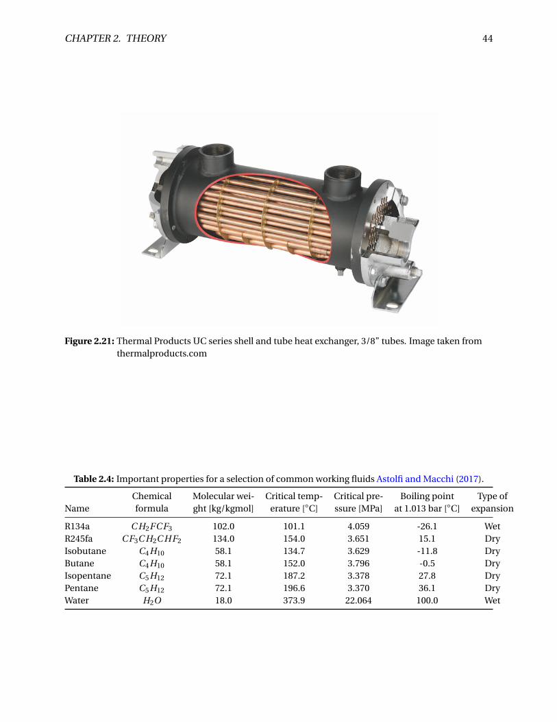
CHAPTER 2. THEORY 44
Figure 2.21: Thermal Products UC series shell and tube heat exchanger, 3/8” tubes. Image taken fromthermalproducts.com
Table 2.4: Important properties for a selection of common working fluids Astolfi and Macchi (2017).
Chemical Molecular wei- Critical temp- Critical pre- Boiling point Type ofName formula ght [kg/kgmol] erature [◦C] ssure [MPa] at 1.013 bar [◦C] expansion
R134a C H2FC F3 102.0 101.1 4.059 -26.1 WetR245fa C F3C H2C HF2 134.0 154.0 3.651 15.1 DryIsobutane C4H10 58.1 134.7 3.629 -11.8 DryButane C4H10 58.1 152.0 3.796 -0.5 DryIsopentane C5H12 72.1 187.2 3.378 27.8 DryPentane C5H12 72.1 196.6 3.370 36.1 DryWater H2O 18.0 373.9 22.064 100.0 Wet
CHAPTER 2. THEORY 45
2.4 Low Temperature Organic Rankine Cycle Working Fluids:
An Annotated Bibliography
2.4.1 Introduction
Following this introduction two texts related to Low Temperature Organic Rankine Cycles Work-
ing Fluids are summarized with short evaluations to underpin their usefulness to this master’s
thesis. The main goal of this annotated bibliography is to give a brief overview of some of the
literature that has been used and referenced in the report on the topic of working fluid selec-
tion, which is commonly considered as the most vital cycle parameter. It should be noted that
work presented by other authors also serve as a basis for answering the thesis objective of eval-
uating thermodynamic feasibility of a power cycle at Tordis qualitatively, specifically by looking
at results from using ORC technology at other application areas with similar thermodynamic
traits as the Tordis wellstream. The summary also gives the reader better context on how other
researchers analyze various ORC applications in regard to working fluid selection. As in any
standard annotated bibliography, a reflection on the texts’ relevance to the project has been
included for each paper that has been reviewed, and the chapter is finalized with a conclusion.
2.4.2 Annotated Bibliography
Saleh, B. et al (2007). Working fluids for low-temperature organic Rankine cycles. In Energy
32 1210-1221. Elsevier.
Saleh, B. et al performed thermodynamic screening of 31 ORC eligible working fluids using
BACKONE equation of state. Their screening process evaluated performance when the cycle
operating conditions were varied from 30◦C to 100◦C. Supercritical pressures were used in a few
cases, but usually the cycle pressure conditions were 20 bars or lower. For subcritical pressures
the working fluid evaluation process proposed includes checking the curvature of the saturated
vapor line in a temperature vs. specific entropy diagram and checking the state of the fluid going
into the turbine inlet. The list of screened fluids includes alkanes and ethers, sometimes fluo-
rinated. The authors have made an effort to match the different working fluids with the most
optimal cycle configuration in order to maximize performance, which means that by example
the cycle configuration used includes an internal heat exchanger when it is seen that the turbine
outlet phase is superheated. The paper points out that the shape of the saturated vapor line in
a Ts-diagram is one of the most important characteristics of an ORC. The operating pressures
are pointed to as another important parameter when it comes to evaluating ORCs, and it is es-
pecially important to identify if the operation is subcritical or supercritical. When an ORC is
operating in the supercritical pressure range it means that the working fluid does not undergo

CHAPTER 2. THEORY 46
phase changes from liquid to vapor, but instead stays in singular state throughout the cycle.
Figure 2.22 shows what Saleh, B. et al calls a b1 cycle. The "b" is used because the curve is bell
T3
T1
s
Figure 2.22: b1 configured ORC
shaped. The initial state shows a working fluid which is saturated at the condenser outlet. It is
then brought from minimum to maximum cycle pressure using the cycle pump, here shown as
state point 2. The working fluid is next heated by heat exchanging with a source fluid under con-
stant pressure condition until gaseous state (3) is reached. The saturated gas is then expanded
down to condenser pressure (4) which is in the liquid-gas region for this working fluid. The
working fluid passes through the condenser at constant pressure, bringing it back to saturated
liquid state at point 1. If a cycle like this has its state point 4 in the superheated vapor region
while keeping everything else the same as before, the configuration is called a "b2"-cycle. A
"b3"-cycle is shown in Figure 2.23. The initial points are at the same states as the previous con-
figurations, but the working fluid is here superheated in the evaporator until state point 3 is
reached. The expansion ends in the gaseous region, just as in cycle configuration b2. Figure
2.24 shows what Saleh, B. et al calls an "o2" cycle. The "o" is here used because the curve shape
is overhanging. The states of the o2 cycle are generally the same as in b2, as seen in the figure.
"o3" is a configuration not shown by figure here, and is an overhanging shaped curve with state
points as in b3. Figure 2.25 shows a supercritical pressure cycle called "s1". Note that no phase
change happens between state point 2 and 3 in this configuration. The end point (4) in Figure
2.25 is in the liquid-vapor region, and in cases where point 4 is in the superheated vapor region
the cycle is called "s2". Equation (2.74) calculates cycle thermal efficiency unless an extra inter-
nal heat exchanger (IHE) is used in the configuration. IHE has been added in cases where the
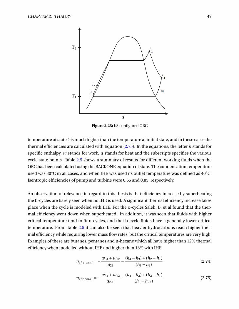
CHAPTER 2. THEORY 47
T3
T1
s
Figure 2.23: b3 configured ORC
temperature at state 4 is much higher than the temperature at initial state, and in these cases the
thermal efficiencies are calculated with Equation (2.75). In the equations, the letter h stands for
specific enthalpy, w stands for work, q stands for heat and the subscripts specifies the various
cycle state points. Table 2.5 shows a summary of results for different working fluids when the
ORC has been calculated using the BACKONE equation of state. The condensation temperature
used was 30◦C in all cases, and when IHE was used its outlet temperature was defined as 40◦C.
Isentropic efficiencies of pump and turbine were 0.65 and 0.85, respectively.
An observation of relevance in regard to this thesis is that efficiency increase by superheating
the b-cycles are barely seen when no IHE is used. A significant thermal efficiency increase takes
place when the cycle is modeled with IHE. For the o-cycles Saleh, B. et al found that the ther-
mal efficiency went down when superheated. In addition, it was seen that fluids with higher
critical temperature tend to fit o-cycles, and that b-cycle fluids have a generally lower critical
temperature. From Table 2.5 it can also be seen that heavier hydrocarbons reach higher ther-
mal efficiency while requiring lower mass flow rates, but the critical temperatures are very high.
Examples of these are butanes, pentanes and n-hexane which all have higher than 12% thermal
efficiency when modelled without IHE and higher than 13% with IHE.
ηther mal =−w34 +w12
q23− (h4 −h3)+ (h2 −h1)
(h3 −h2)(2.74)
ηther mal =−w34 +w12
q2a3− (h4 −h3)+ (h2 −h1)
(h3 −h2a)(2.75)

CHAPTER 2. THEORY 48
T3
T1
s
Figure 2.24: o2 configured ORC
T3
T1
s
Figure 2.25: s1 configured ORC

CHAPTER 2. THEORY 49
Table 2.5: Selection of numerical results taken from Saleh et al. (2007) for different working fluidsubstances. Both basic ORC and ORC with IHE calculated using BACKONE EOS.
Substance Cycle Tc pc T3 T4 pmi n pmax m ηther mal ηther mal
type [◦C] [bar] [◦C] [◦C] [bar] [bar] [kg/s] [%] (IHE)[%]
R125 b1 66.18 36.30 40.06 30.0 15.64 20.0 400.37 2.32 —R125 b3 66.18 36.30 100.0 91.92 15.64 20.0 246.30 2.36 3.36R218 o2 71.89 26.80 58.99 33.68 10.04 20.0 238.23 5.22 —R218 o3 71.89 26.80 100.0 82.86 10.04 20.0 151.55 5.15 7.50R143a b1 72.73 37.64 43.59 30.0 14.40 20.0 197.92 3.14 —R143a b3 72.73 37.64 100.0 87.37 14.40 20.0 127.89 3.31 4.36R32 b1 78.11 57.83 31.36 30.0 19.31 20.0 1062.6 0.36 —R32 b3 78.11 57.83 100.0 97.75 19.31 20.0 682.78 0.42 0.53RE125 b2 81.34 33.51 57.67 31.50 10.11 20.0 145.17 5.67 —RE125 b3 81.34 33.51 100.0 79.04 10.11 20.0 103.11 5.77 7.34R1270 b1 92.42 46.65 48.54 30.0 13.09 20.0 69.334 4.28 —R1270 b3 92.42 46.65 100.0 81.28 13.09 20.0 49.109 4.53 5.51R290 b1 96.65 42.50 57.14 30.0 10.79 20.0 48.776 5.91 —R290 b3 96.65 42.50 100.0 76.02 10.79 20.0 36.100 6.11 7.32R134a b1 101.03 40.56 67.75 30.0 7.722 20.0 68.55 7.74 —R227ea o2 101.74 29.29 83.88 44.19 5.331 20.0 81.523 9.20 —R152a b1 113.5 44.95 72.59 30.0 6.888 20.0 38.503 8.82 —R152a b3 113.5 44.95 100.0 53.84 6.888 20.0 31.987 9.22 9.71RC318 o2 115.23 27.78 98.93 54.72 3.68 20.0 66.828 10.97 12.09RC318 o3 115.23 27.78 100.0 56.38 3.68 20.0 68.694 10.55 11.75CF3I b1 123.29 39.53 85.24 30.0 5.652 20.0 97.043 10.63 —CF3I b3 123.29 39.53 100.0 39.60 5.652 20.0 86.917 10.93 —RC270 b3 124.65 54.90 100.0 41.63 8.227 20.0 24.713 8.86 —R236fa o2 125.55 32.00 100.0 48.61 3.240 19.35 47.313 11.63 12.14RE170 b1 126.85 52.40 75.10 30.00 6.733 20.0 63.068 9.38 —RE170 b3 126.85 52.40 100.0 53.03 6.733 20.0 54.488 9.68 10.13RE245mc o2 133.68 28.87 100.0 54.50 2.416 14.88 42.549 11.84 12.72R600a o2 135.05 36.50 100.0 45.33 4.038 19.98 20.423 12.12 12.43R236ea o2 139.22 34.12 100.0 53.92 2.438 15.74 41.361 12.02 12.83RE134 o2 147.1 42.28 100.0 41.04 2.501 16.66 32.149 12.56 —C5F12 o2 148.85 20.40 100.0 72.76 1.037 7.66 67.15 10.49 13.10R600 o2 152.05 38.00 100.0 48.43 2.850 15.29 17.746 12.58 13.04R245fa o2 154.05 36.40 100.0 50.70 1.801 12.67 33.424 12.52 13.07R338mccq o2 158.8 27.26 100.0 63.08 1.117 8.428 46.486 11.84 13.30neo-C5 H12 o2 160.65 32.00 100.0 58.92 2.001 11.16 20.426 12.20 13.37RE347mcc o2 164.55 24.76 100.0 66.98 0.959 7.103 45.263 11.72 13.49RE245 o2 170.88 30.48 100.0 58.47 1.040 8.198 42.549 12.59 13.59R245ca o2 174.42 39.25 100.0 53.75 1.230 9.343 30.548 12.79 13.47R601a o2 187.75 33.86 100.0 58.47 1.098 7.223 17.439 12.75 13.76R601 o2 196.5 33.70 100.0 57.74 0.828 5.963 16.331 12.91 13.84n-hexane o2 234.67 30.10 100.0 61.89 0.250 2.481 15.853 13.00 14.14
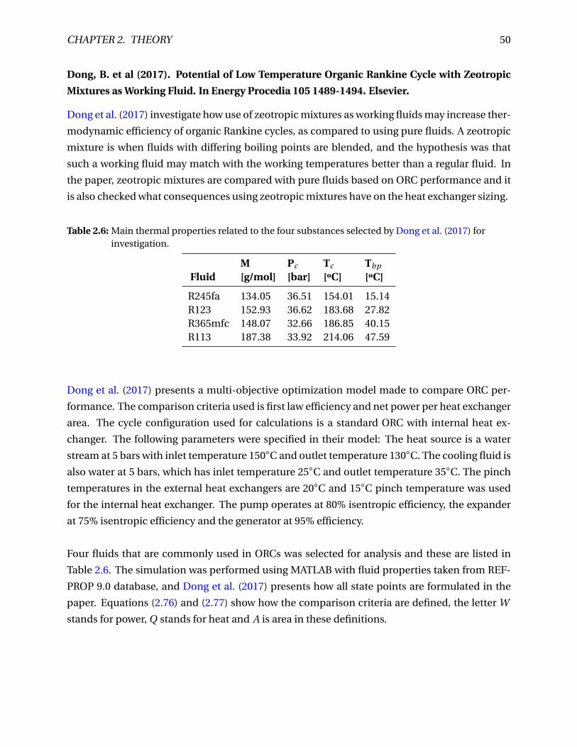
CHAPTER 2. THEORY 50
Dong, B. et al (2017). Potential of Low Temperature Organic Rankine Cycle with Zeotropic
Mixtures as Working Fluid. In Energy Procedia 105 1489-1494. Elsevier.
Dong et al. (2017) investigate how use of zeotropic mixtures as working fluids may increase ther-
modynamic efficiency of organic Rankine cycles, as compared to using pure fluids. A zeotropic
mixture is when fluids with differing boiling points are blended, and the hypothesis was that
such a working fluid may match with the working temperatures better than a regular fluid. In
the paper, zeotropic mixtures are compared with pure fluids based on ORC performance and it
is also checked what consequences using zeotropic mixtures have on the heat exchanger sizing.
Table 2.6: Main thermal properties related to the four substances selected by Dong et al. (2017) forinvestigation.
M Pc Tc Tbp
Fluid [g/mol] [bar] [ºC] [ºC]
R245fa 134.05 36.51 154.01 15.14R123 152.93 36.62 183.68 27.82R365mfc 148.07 32.66 186.85 40.15R113 187.38 33.92 214.06 47.59
Dong et al. (2017) presents a multi-objective optimization model made to compare ORC per-
formance. The comparison criteria used is first law efficiency and net power per heat exchanger
area. The cycle configuration used for calculations is a standard ORC with internal heat ex-
changer. The following parameters were specified in their model: The heat source is a water
stream at 5 bars with inlet temperature 150◦C and outlet temperature 130◦C. The cooling fluid is
also water at 5 bars, which has inlet temperature 25◦C and outlet temperature 35◦C. The pinch
temperatures in the external heat exchangers are 20◦C and 15◦C pinch temperature was used
for the internal heat exchanger. The pump operates at 80% isentropic efficiency, the expander
at 75% isentropic efficiency and the generator at 95% efficiency.
Four fluids that are commonly used in ORCs was selected for analysis and these are listed in
Table 2.6. The simulation was performed using MATLAB with fluid properties taken from REF-
PROP 9.0 database, and Dong et al. (2017) presents how all state points are formulated in the
paper. Equations (2.76) and (2.77) show how the comparison criteria are defined, the letter W
stands for power, Q stands for heat and A is area in these definitions.

CHAPTER 2. THEORY 51
Table 2.7 displays how the use of mixtures can improve cycle performance, note that the bi-
nary mixtures presented are the optimal mass fractions of each fluid combination. It is however
apparent that because of a bigger portion of the heat transfer from the heat source happens dur-
ing working fluid phase change, the required heat exchangers must be a lot larger and especially
so for the IHE. Figure 2.26 shows the results from the heat exchanger calculations graphically,
and looking to the rightmost plot it is clear that the most cost-effective performance is when
pure fluids are used as working fluid. In other words it means that you cannot reach the highest
cycle efficiency and cost-effective performance simultaneously.
η= Wg ener ator −Wpump
Qevapor ator(2.76)
ε= Wnet
Atot al= Wg ener ator −Wpump
Aevapor ator + Acondenser + AI HE(2.77)
The findings are of significant interest to this master’s thesis, because it shows that zeotropic
mixtures could be used to get higher cycle efficiency if a certain output threshold can not be
reached with pure fluids. On the other hand, it will be a bad idea if the threshold can already
be met, since the heat exchangers will be more expensive. A practical example related to Tordis
ORC would be if pure fluids used as working fluids made for lower net power output than re-
quired for a specific purpose, for example boosting. In such a scenario zeotropic mixtures can
be considered as a substitute to meet the output requirement, despite the fact that the heat
exchangers needs to be sized up.
Table 2.7: Results taken from Dong et al. (2017). Shows how cycle efficiency can be improved usingzeotropic (binary) mixtures.
Mass Pevap Pcond Pr ati o T g r adevap
T g r adcond
Wg en Wpump η
Fluid fraction [bar] [bar] [-] [°C] [°C] [W] [W] [%]
R245fa 1 19.0 3.9 4.9 0 0 210.1 15.3 9.10R123 1 11.3 2.4 4.7 0 0 212.1 9.0 9.48R365mfc 1 8.7 1.6 5.3 0 0 214.2 7.2 9.67R113 1 6.3 1.3 5.0 0 0 214.4 5.2 9.77R123/R365mfc 0.32/0.68 9.7 1.9 5.2 0.62 1.13 216.3 7.9 9.73R245fa/R123 0.21/0.79 14.0 2.8 5.0 2.84 3.00 219.9 11.4 9.74R365mfc/R113 0.40/0.60 7.2 1.4 5.2 0.81 0.47 216.2 6.0 9.82R123/R113 0.26/0.74 8.2 1.6 5.3 3.75 4.19 225.5 6.9 10.21R245fa/R365mfc 0.30/0.70 12.4 2.1 5.8 5.02 6.34 229.2 10.3 10.23R245fa/R113 0.32/0.68 12.4 2.1 5.8 12.43 13.00 240.3 10.6 10.73

CHAPTER 2. THEORY 52
Figure 2.26: Effect of using binary working fluid on heat exchanger design. Taken from Dong et al.(2017).
2.4.3 Annotated Bibliography Result Summary and Conclusion
Saleh et al. (2007) investigated the thermal efficiencies of using various fluids as working fluids
in low temperature ORCs with BACKONE EOS. The results varied from ηther mal = 0.36% for R32
to ηther mal = 14.14% for n-hexane. The model used the most fitting cycle configuration for every
investigated fluid and added internal heat exchanger in cases where the gas at expander outlet
was superheated. Comparing results with and without IHE it can be seen that the efficiency
increase is usually less than a percent when IHE is added. Dong et al. (2017) showed that using
multi-component working fluids may improve thermal efficiencies of low temperature Rankine
cycles, proposing that the wide usage of singular component fluids in the present industry may
be inefficient. The analysis focused on investigating possible issues with heat exchanger sizing
when diverging from standard working fluids to see if it would pay off or not. It was shown that
using binary mixtures as working fluids could increase the thermal efficiency of the cycles with
around one percent, but the effective heat exchanger areas would be increased by significant
margin. It was concluded that usage of pure fluids would be more cost effective in general, es-
pecially in cases when IHE is used.
The literature review of low temperature ORC working fluid screening showed that even for
"bad" heat sources it is possible to get a reasonable thermal energy conversion efficiency. This is
seen as a very promising find, as the Tordis wellstream poses a large energy potential due to the
high mass rates, despite its low average temperature of around 75◦C. The results from the other
researchers showed that conversion efficiencies of 8-12% can be reasonably expected from low
temperature sources, if the right fluid is chosen as working media. Covering the requirements
for boosting is defined as a criterium for determining if use of ORC at Tordis is viable. If it is
assumed that the wellstream cools from 75◦C to 20◦C by heat exchange with a working fluid, the

CHAPTER 2. THEORY 53
total energy transfer was shown earlier as 46.5 MW. If the ORC converts with 9% or better thermal
efficiency it will be able to cover the Tordis boosting power consumption at 4MW, which means
it is plausible that usage of ORC may be feasible, from a qualitative standpoint. Further on in
this thesis it is investigated whether energy transfer of 46.5 MW would be realistically possible
or not, by the use of more rigorous models.

Chapter 3
Methodology and Model Descriptions
3.1 Model for calculation of Raw Power Available
The model for the raw power estimation consists of multiple parts, all of which will be explained
in detail in this section. Figure 3.2 is a picture taken of the Aspen HYSYS portion of the model,
that is behind all the calculations and estimated results. In addition, Excel VBA code has been
written to efficiently run the model with varying inputs for sensitivity analysis, see Appendix A.
It should be noted that the VBA is a modified version of a script used in Gleditsch (2017) for
sensitivity analysis of the phase effect on raw power available. The necessary inputs to run the
model are hydrocarbon composition, flow rates, wellhead and surface process PT conditions.
The surface process PT conditions are required to estimate GOR, WC and produced volume
rates at standard conditions. Since Excel VBA can communicate with HYSYS, it was found con-
venient to limit all inputs to be made in a spreadsheet, keeping the manual work in HYSYS to a
minimum.
54

CHAPTER 3. METHODOLOGY 55
StartExcel
macro
Load inputsfrom Excel toAspen HYSYS
Value for GORloaded into SS_GOR
WH and surfaceprocess pressuresand temperaturesloaded to streamsInitialComp, 1 and2Composition and
initial flow rateloaded to the ma-terial stream Initial-Comp
Determine gas andoil compositionat wellhead P/T.
Setting determined WHcompositions as input to
the surface processing.
Streams g-0 and o-0becomes copies ofstreams g-i and o-i
This step is only required ifgas and oil compositions arenot separately available, thenseparator V-102 makes an esti-mation from combined comp.
Flow rates are de-termined to match
specified GOR
HYSYS changes flowrate of g-0 itera-tively using adjust
Raw heat potential isestimated based on the
resulting composition andflow rate of Inlet stream.
Specified tempera-ture drop dT loadedto cooler E-104
Stream FEED-1 be-comes a copy ofstream Inlet stream.
Output HYSYS esti-mates back to Excel
Volumetric flow rate,raw heat flow rate,mass enthalpy andZ-factor correspond-ing to the specifiedGOR and dT aresaved.
Is simulationfinished?
Update all valuescorrespondingto next month.
Endprogram
No
Yes
Figure 3.1: Flowchart for raw power model that estimates raw power potential over time based on afields production history using monthly data.

CHAPTER 3. METHODOLOGY 56
Figu
re3.
2:R
awp
ower
mo
del
.Sn
apsh
otf
rom
Asp
enH
YSY
S.
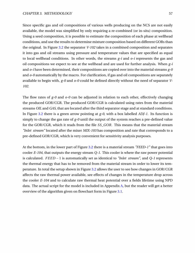
CHAPTER 3. METHODOLOGY 57
Since specific gas and oil compositions of various wells producing on the NCS are not easily
available, the model was simplified by only requiring a re-combined (or in-situ) composition.
Using a seed composition, it is possible to estimate the composition of each phase at wellhead
conditions, and use the results to determine mixture composition based on different GORs than
the original. In Figure 3.2 the separator V-102 takes in a combined composition and separates
it into gas and oil streams using pressure and temperature values that are specified as equal
to local wellhead conditions. In other words, the streams g-i and o-i represents the gas and
oil compositions we expect to see at the wellhead and are used for further analysis. When g-i
and o-i have been determined, their compositions are copied over into the material streams g-0
and o-0 automatically by the macro. For clarification, if gas and oil compositions are separately
available to begin with, g-0 and o-0 could be defined directly without the need of separator V-
102.
The flow rates of g-0 and o-0 can be adjusted in relation to each other, effectively changing
the produced GOR/CGR. The produced GOR/CGR is calculated using rates from the material
streams OIL and GAS, that are located after the third separator stage and at standard conditions.
In Figure 3.2 there is a green arrow pointing at g-0, with a box labelled ADJ-1. Its function is
simply to change the gas rate of g-0 until the output of the system reaches a pre-defined value
for the GOR/CGR, which it reads from the file SS_GOR. This means that the material stream
"Inlet stream" located after the mixer MIX-103 has composition and rate that corresponds to a
pre-defined GOR/CGR, which is very convenient for sensitivity analysis purposes.
At the bottom, in the lower part of Figure 3.2 there is a material stream "FEED-1" that goes into
cooler E-104, that outputs the energy stream Q-1. This cooler is where the raw power potential
is calculated. F EED − 1 is automatically set as identical to "Inlet stream", and Q-1 represents
the thermal energy that has to be removed from the material stream in order to lower its tem-
perature. In total the setup shown in Figure 3.2 allows the user to see how changes in GOR/CGR
affects the raw thermal power available, see effects of changes in the temperature drop across
the cooler E-104 and to calculate raw thermal heat potential over a fields lifetime using NPD
data. The actual script for the model is included in Appendix A, but the reader will get a better
overview of the algorithm given on flowchart form in Figure 3.1.

CHAPTER 3. METHODOLOGY 58
3.2 The Subsea ORC Model for Tordis
A model has been made to determine the net output power potential of a subsea organic Rank-
ine cycle based on the produced fluids from Tordis, and to get a rough overview of the equip-
ment sizes necessary. The following constraints apply. Tordis is currently producing 31.5 kg /s
of condensate and 161 kg /s of water. The wellhead temperature ranges between 50 - 75 ◦C,
and the wellhead pressures are kept between 20 - 50 bara. The ambient sea water tempera-
ture ranges between 6 - 9 ◦C at the wellheads, which are located roughly 250 meters below the
surface of the sea. Since specific details related to the cycle components are yet to be deter-
mined, typical values for the unknowns have to be assumed to get an approximate model that
will give a larger understanding of which cycle components are necessary and their sizes. The
basic ORC configuration consisting of an expander, turbine, pump, condenser and an evapora-
tor has been presented earlier in this thesis, and is used as the starting point for this evaluation.
The following common assumptions for ORC modelling has been taken from peer-reviewed lit-
erature and can be found at multiple sources. It is assumed that the cycle operates at steady
state, that the isentropic efficiency of the expander is 85%, an isentropic efficiency of the pump
of 80% and mechanical efficiency of the turbine is 98%-100%. In thermal analysis, the point
where the temperature difference between hot and cold fluid is at its minimum is called a pinch
point. It is common to model heat exchangers in ORCs with 5◦C at pinch points, as it is assumed
that the temperature difference between the streams needs to be at least 5◦C to get meaningful
heat transfer. When it comes to the cycle pressure it is always ensured that the expander outlet
pressure is at a level where the vapor fraction of the working fluid is 100%, since having liquid
droplets in the expander will erode the turbine blades. The pressure and temperature at the
condenser outlet are adjusted to a level where the vapor fraction of the working fluid is zero, so
that no gas passes through the pump and also to ensure that the cycle operates below the critical
point. This means that the pump duty will be adjusted accordingly and have direct effect on the
cycle net power output.
The most important part for any ORC model is to select a fitting working fluid to run in the cycle.
The methodology for selecting a proper working fluid for the model is explained in Section 3.3,
and the fluid screening process is based upon the restraints of the model presented here. Since
the Tordis wellhead temperatures are reported as ranging between 50 - 75◦C, it would make
sense to at least include the entire interval in the analysis as a minimum. It is also interesting
to look into the effects of higher cycle inlet temperatures since other fields produce fluids with
higher enthalpy than Tordis, so the temperature interval from 50 to 115 ◦C is therefore exam-
ined for the working fluid selection. As mentioned, the sea water temperature in the area is
reported as ranging between 6 - 9 ◦C, so the ORC is modeled with a fixed value of 9 ◦C ambient
temperature for cooling purposes.

CHAPTER 3. METHODOLOGY 59
3.3 Evaluation of Potential Working Fluids
The working fluids used for comparison are chosen from the Aspen HYSYS components list in
the Basis Environment, which contains in total 37 fluids that are suitable for removing heat by
evaporation close to the normal boiling point. To make the initial working fluid comparison ef-
ficient, an Excel VBA that interacts with Aspen HYSYS was written to help with the process. The
VBA makes it possible to choose a working fluid substance and run a Rankine cycle simulation
using HYSYS while saving data to an Excel spreadsheet, working only from the Excel interface.
As an example, the author could select n-Butane as a working fluid and by the press of a button
HYSYS would calculate Rankine cycle solutions for the temperature pre-defined range 50 to 115◦C and save the parameters of interest for each iteration. The VBA can be found in Appendix B,
and was used to get data points for several of the trend plots contained in the results section.
For a low temperature organic Rankine cycle, it is possible to either use a hydrocarbon or re-
frigerant substance as the working fluid. Refrigerants are sometimes chosen due to being non-
flammable, but the potential environmental impact is much larger than for hydrocarbon work-
ing fluids. The working fluid selection has been performed based on two primary criteria, being
performance and level of environmental risk. The HYSYS model is based on the constraints
listed in Section 3.2 and was used to vet the heat transfer fluids contained in the HYSYS basis
environment component list, computing net power output and thermal efficiency over the heat
source temperature interval 50-115◦C. After seeing the performance of each fluid ranked from
best to worst, the environmentally harmful ones have been removed until we have a ranking
with less environmental risk. Table 3.1 contains an overview over candidate refrigerant fluids
that have low boiling points and could possibly work in the ORC. Additional fluids proposed by
the paper Working fluids for low-temperature Rankine cycles by Saleh et al. (2007) were added
to the list of potential candidates, here listed in Table 3.2. Note that some of the fluids in Table
3.2 could not be found in the Aspen HYSYS component list, and was therefore simulated using
a basic ORC model in Aspen Plus V9 instead.
Some of the boundary conditions for the fluid selection model affect the various working flu-
ids differently. Since the model assumes heat exchangers with 5◦C pinch, some fluids may be at
the point of saturation and others may be completely dry or wet depending on the critical points
of the fluid. In practice this will for example mean that the working fluid leaving the condenser
will be at 14 ◦C when the sea water temperature is 9 ◦Celsius, no matter what the working fluid is.
The working fluid gas leaving the evaporator is defined in the same way, being 5 ◦Celsius lower
than wellhead temperature. Because of these specifications it should be noted that some poten-
tial fluids will be superheated when passing through the expander and some will be subcooled
when passing through the pump, since all the fluids have different phase curves. The pressure

CHAPTER 3. METHODOLOGY 60
changes across the heat exchangers on the working fluid side were defined as fixed values of
1 bara shell side in this analysis and the isentropic efficiencies of pump and turbine are equal
to unity for the fluid screening only. The wellstream supplying the raw thermal energy has the
composition shown in Table 4.1 and the tube side pressure drop in the evaporator was defined
as 3 bara.

CHAPTER 3. METHODOLOGY 61
Table 3.1: Possible heat transfer fluids contained in the HYSYS database.
Full Name Formula Norm. TBP [◦C]Refrig-11 CCl3F 24Refrig-12 CCl2F2 -30Refrig-13 CClF3 -81Refrig-14 CF4 -128Refrig-22 CHClF2 -41Refrig-23 CHF3 -82Refrig-50 CH4 -162Refrig-113 C2Cl3F3 48Refrig-114 C2Cl2F4 4Refrig-170 C2H6 -89Refrig-290 C3H8 -42Refrig-500 - -34Refrig-502 - -45Refrig-503 - -88Refrig-600 C4H10 -1Refrig-702 H2 -253Refrig-704 He -269Refrig-717 NH3 -33Refrig-718 H2O 100Refrig-720 Ne -246Refrig-728 N2 -196Refrig-729 - -195Refrig-732 O2 -183Refrig-740 Ar -186Refrig-744 CO2 -79Refrig-1150 C2H4 -104Refrig-1270 C3H6 -48Refrig-13B1 CBrF3 -58Refrig-142b C2H3ClF2 -10Refrig-152a C2H4F2 -25Refrig-600a C4H10 -12Refrig-702a H2 -253Refrigerant_113 C2Cl3F3 48Refrigerant_125 C2HF5 -48Refrigerant_152 C2H4F2 11Refrigerant_133a C2H2ClF3 6Refrigerant_134a C2H2F4 -26Refrigerant_216ca C3Cl2F6 36

CHAPTER 3. METHODOLOGY 62
Table 3.2: Possible working fluids especially suited for low-temperature ORCs, presented in Saleh et al.(2007).
Full Name FormulaR32 CH2F2R41 CH3FR125 C2HF5R134a C2H2F4R143a C2H3F3R152a C2H4F2R218 C3F8R227ea C3HF7R236ea C3H2F6R245ca C3H3F5R245fa C3H3F5RC-270 Cyclo-PropaneR290 PropaneRC318 Cyclo-C4F8R338mccq C4H2F8R600 n-butaneR600a Iso-butaneR1270 C3H6CF3I CF3IC5F12 C5F12R601 n-pentaneR601a Iso-pentaneneo-C5H12 Neo-pentanen-C6H14 n-hexaneRE125 C2HF5ORE134 C2H2F4ORE170 C2H6ORE245 C3H3F5ORE245mc C3H3F5ORE347mcc C4H3F7O

CHAPTER 3. METHODOLOGY 63
3.4 Shell and Tube Evaporator Model
Calculating the heat exchanger properties should be performed using an iterative process. This
is mainly because the heat transfer coefficients are a function of the Reynolds numbers, which
means the flow velocities and hence the cross sectional areas have to be specified initially. Figure
3.3 shows the algorithm that is used for thermal design of a shell and tube evaporator.
Read base inputs
Geometric specifi-cations of tube OD,tube pitch and tub-ing pattern is de-fined up front.
TEMA type, buildmaterial and baffleconfiguration mustbe chosen initially.
Determine heatload Q tubeside
and shellside.
Calculate effective cor-rected temperaturedifference TC MT D
Pick heat exchangerconfiguration based
on value for U .
Output cur-rent estimates
Number of shells,tubing and theirsizes. Number ofbaffles, passes, ex-cess fouling and ex-cess area is of spe-cial interest.
Have resultsconverged?
Checking if currentheat exchanger se-lection satisfies theinitial data input.
Calculate new val-ues for heat transfercoefficients α and U
End
No
Yes
Figure 3.3: Flowchart for thermal modeling of S&T heat exchangers. Based on the algorithm shown inNitsche and Gbadamosi (2016).

CHAPTER 3. METHODOLOGY 64
3.5 Passive Cooling Manifold Model
In order to estimate an approximate size of a passive cooling system, a simple model for calcu-
lating the natural convection effect between the sea and cycle working fluid has been developed.
The aim is to see how much piping would be needed to get the required cooling duty, and note
that pipe bends are not accounted for in this model. Figure 3.4 illustrates the expected thermal
resistance for single wall-section of tubing when it is made of super duplex with no coating.
T∞, w f
RW F RSE A
T∞, SE A
RSD
Ti To
W or ki ng f lui d Super Dupl ex Sea
Figure 3.4: Illustration of equivalent thermal resistance for the modeled system. Red color points toconvective thermal resistance of the fluid-solid interfaces. Thermal resistance of the solidtube material Super Duplex is shown in black.
3.5.1 Forced Convective Heat Transfer
Forced convective heat transfer from the working fluid can be expressed with Newton’s Law of
Cooling, here formulated in Equation (3.1). Figure 3.5 illustrates convection happening at the
contact surface between the working fluid and the super duplex tube. The convection coeffi-
cient α1 is a function of surface geometry, fluid properties and velocity. A term for the convec-
tive thermal resistance is shown in Equation (3.2), which can be used to express the heat flow in
terms of temperature difference and thermal resistance as in Equation (3.3).
Q =α1 A1(T∞, w f −Ti ) (3.1)
TiMoving fluid
T∞, w f Q
Figure 3.5: Convection on interface between the working fluid and inner side of pipe wall.
RW F = 1
α1 A1(3.2)

CHAPTER 3. METHODOLOGY 65
Q = T∞, w f −Ti
RW F(3.3)
The heat transfer coefficient α1 has to be determined, and as seen by Equation (3.4), it can be
defined by the Nusselt number Nu1, the pipe diameter D and the thermal conductivity of the
fluid κ1. A value for the pipe diameter can be selected based on available process drawings or
assumed, and finding the thermal conductivity of the working fluid can be done with Aspen
HYSYS. The Nusselt number has to be calculated with empirical correlations, and as mentioned
earlier in the thesis, there exists a number of Nu-correlations valid for a range of different ap-
plications. The definitions given by Equation (3.5) and Equation (3.6) are suitable for laminar
flow within a circular tube with constant wall temperature according to the publication Sub-
sea Pipeline Design, Analysis, and Installation by Bai and Bai (2014). If the internal pipe flow
conditions are turbulent, the Gnielski empirical formula given in Equation (3.7) can be used.
α1 = Nu1κ1
D(3.4)
Nu1 = 3.66+ 0.0668RePr (D/L)
1+0.04[RePr (D/L)]2/3,
Re < 2300
Pr ≥ 5(3.5)
Nu1 = 1.86(RePr
L/D)1/3(
µb
µw)0.14,
Re < 2300
0.6 < Pr < 5
0.0044 < µb
µw< 9.75
(3.6)
Nu1 = ( f /8)(Re −1000)Pr
1+12.7( f /8)1/2(Pr 2/3 −1),
3000 ≤Re ≤ 5 ·106
0.5 ≤Pr ≤ 2000(3.7)
f = (0.79l n(Re)−1.64)−2 (3.8)
Nomenclature for Chapter 3.5.1
Q Rate of heat flow (W)
α1 Heat transfer coefficient (W/m2 ·K)
A1 Pipe internal surface contact area (m2)
T∞, w f Working fluid temperature (K)
Ti Temperature on pipe internal surface (K)
RW F Working fl. thermal resistance (K/W)
κ1 Working fl. thermal conductivity
(W/m ·K)
Nu1 Nusselt number, forced convection [−]
D Pipe diameter (m)
L Pipe length (m)
Re Reynolds number [−]
Pr Prandtl number [−]
µb Viscosity at fluid temperature (Pa · s)
µw Viscosity at wall temperature (Pa · s)
f Friction factor [−]

CHAPTER 3. METHODOLOGY 66
Q
Ti
T∞, w f Q
RSD
To
α1
T∞, SE Aα2
Figure 3.6: Illustration of complete heat transfer process through super duplex pipe wall.
3.5.2 Natural Convective Heat Transfer
The thermal energy is then conducted through the solid pipe wall and is eventually transferred
to the surrounding sea water via natural convection, as illustrated in Figure 3.6. The expression
for the resistance to convective heat transfer on the interface between super duplex and water
on the outside of the pipe, RSE A, can be formulated in the same way as for the inner side, here
given by Equations (3.9)-(3.11).
Q =α2 A2(To −T∞, SE A) (3.9)
RSE A = 1
α2 A2(3.10)
Q = To −T∞, SE A
RSE A(3.11)
The convection on the interface between outer pipe and the sea happens naturally, which means
the expression for the Nusselt number is different from the equations given in Section 3.5.1. It is
also important to distinguish between horizontal and vertical systems when analyzing natural
convection, Equation (3.12) defines the heat transfer coefficient for vertical systems and Equa-
tion (3.13) defines it for horizontal systems. The Nusselt number correlation given in Equation
(3.14) is suitable for horizontal cylinders (Churchill and Chu (1975a)). For reference it can be
noted that for vertical systems a more accurate expression is given by Equation (3.15) (Churchill
and Chu (1975b)), but since we are modeling without bends this final correlation is not used in
our model.
α2 = Nu2κ2
L(3.12)

CHAPTER 3. METHODOLOGY 67
α2 = Nu2κ2
D(3.13)
Nu2 =√
0.60+0.387(Ra
[1+ (0.559/Pr )9/16]16/9)1/6 (3.14)
Nu2 =√
0.825+0.387(Ra
[1+ (0.437/Pr )9/16]16/9)1/6 (3.15)
Nomenclature for Chapter 3.5.2
Q Rate of heat flow (W)
α2 Heat transfer coefficient (W/m2 ·K)
A2 Pipe external surface contact area (m2)
T∞, SE A Average temperature of sea (K)
To Temperature on pipe external surface (K)
RSE A Brine thermal resistance (K/W)
κ2 Brine thermal conductivity (W/m ·K)
Nu2 Nusselt number, natural convection [−]
D Pipe diameter (m)
L Pipe length (m)
Pr Prandtl number [−]
3.5.3 Equivalent Thermal Resistance
To determine the equivalent thermal resistance of the system, we use the fact that the heat en-
ergy is conserved. Note that we look at the system as a whole, thus the expressions for heat flow
via conduction takes into account the cylindrical geometry of pipes, which is somewhat differ-
ent from when heat flow through flat plates is considered. In this regard note that the parameter
inside the natural log is the fraction between outer and inner pipe radius.
Q =α1 A1(T∞, w f −Ti )
= 2πLkSD(Ti −To)
l n( rori
)
=α2 A2(To −T∞, SE A)
(3.16)
With two steps, we formulate the expressions in Equation (3.16) into terms of thermal resistance
as shown by Equations (3.17)-(3.18). Since the resistances act as a series, we can calculate the
equivalent thermal resistance simply by adding each individual contribution, as in Equation
(3.19). Figure 3.4 visualizes how the different thermal resistances relate to each other as a series,
but the figure does not illustrate how significant the different resistances are in relation to each
other. For example, the resistance related to convection is often negligible in comparison to
the resistance to conduction. If one decides to ignore the resistance to convection when setting
up the equations, they become much easier to solve and knowledge of the temperature on the
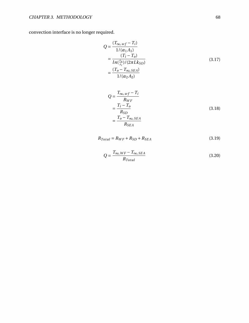
CHAPTER 3. METHODOLOGY 68
convection interface is no longer required.
Q = (T∞, w f −Ti )
1/(α1 A1)
= (Ti −To)
ln( rori
)/(2πLkSD )
= (To −T∞, SE A)
1/(α2 A2)
(3.17)
Q = T∞, w f −Ti
RW F
= Ti −To
RSD
= To −T∞, SE A
RSE A
(3.18)
RTot al = RW F +RSD +RSE A (3.19)
Q = T∞,W F −T∞, SE A
RTot al(3.20)

Chapter 4
Numerical Results
4.1 Tordis Raw Power Potential Variation with Time
The estimates from the raw power potential simulation over time have been made as realistic
as possible by using the Excel sheet 20170402_NCS_Production_Data.xls as prepared by Prof.
Milan Stanko, which summarizes production data from fields on the NCS. Table 4.1 contain
the mol percentages used to represent the composition of the fluid produced from Tordis and
compositional changes over time has been accounted for with a recombinational procedure to
match the field GOR and WC for each iteration of the simulation. Aspen HYSYS estimated the
properties of the hypotheticals based on molecular weight and density as specified in Table 4.2.
It should be noted that a big disadvantage of using hypotheticals estimated this way by equa-
tion of state is that one can not be 100% certain that the PVT properties are reproduced properly
unless laboratory measurements are performed. Higher accuracy would be achieved by per-
forming a fluid characterization study to estimate binary interaction parameters that reproduce
the experimental data.
As the excel sheet 20170402_NCS_Production_Data.xls contains information about monthly av-
erage GOR, WC and oil production, it was possible to perform the simulation with correct aver-
aged monthly fluid volumes. However, HYSYS struggled to reach convergence when adjusting
multiple parameters at once and in this case it was necessary to adjust both the GOR to be cor-
rect for each monthly input (one iteration) and the total amount of oil produced to match a
value. Therefore, it was opted to have the volume matching done by iterating through Excel
VBA in the form of two while-loops, and leaving GOR matching to HYSYS. Script is found in Ap-
pendix A.1.1. Once the model reaches match for both GOR and oil rate, the amount of water
was calculated based on the value for average WC for that month and the actual liquid volume
flow from HYSYS. The estimated amount of water was then added to and mixed with the hydro-
carbon rates at wellhead conditions, before a heat energy calculation was run with ∆T = 50◦C
69

CHAPTER 4. RESULTS 70
across the cooler. Note that the composition used for water was simply H2O, and not brine.
Table 4.1: Tordis hydrocarbon composition. Data supplied by Equinor ASA.
Ni tr og en 0.60 mol −%CO2 0.27 mol −%Methane 36.61 mol −%Ethane 7.07 mol −%Pr opane 6.89 mol −%i −But ane 1.19 mol −%n −But ane 3.49 mol −%i −Pent ane 1.28 mol −%n −Pent ane 1.79 mol −%n −Hexane 2.46 mol −%n −Hept ane 3.65 mol −%n −Oct ane 4.27 mol −%n −Nonane 2.73 mol −%C 10−C 12 6.46 mol −%C 13−C 15 4.95 mol −%C 16−C 18 3.80 mol −%C 19−C 22 3.73 mol −%C 23−C 25 2.05 mol −%C 26−C 30 2.41 mol −%C 31−C 36 1.79 mol −%C 37−C 46 1.50 mol −%C 47−C 80 1.01 mol −%
Table 4.2: Tordis hypothetical components properties estimated in Aspen HYSYS based on molecularweight and density.
Critical Properties
Molecular Density Normal Temper- Pressure Volume Acent-Hypothetical Weight [kg/m3] Boiling Pt [◦C] ature [◦C] [kPa] [m3/kgmole] ricity
C10-C12 146.56 799.40 181.78 373.60 2442.35 0.557 0.406C13-C15 189.44 825.30 231.65 423.42 2106.41 0.675 0.495C16-C18 235.83 846.00 286.52 473.90 1766.39 0.832 0.608C19-C22 281.98 865.80 334.87 517.69 1535.98 0.978 0.713C23-C25 330.56 882.90 380.80 557.86 1346.96 1.128 0.822C26-C30 385.36 899.00 428.48 598.32 1175.94 1.295 0.943C31-C36 461.50 917.90 489.96 649.20 988.25 1.524 1.111C37-C46 567.19 939.80 569.59 713.69 788.60 1.839 1.344C47-C80 783.00 974.50 721.35 834.86 500.50 2.485 1.770

CHAPTER 4. RESULTS 71
Table 4.3: Processing modelled as a simple three stage separator train
Wellhead Temperature 75 [◦C]Wellhead Pressure 40 [bar]1st Stage Temperature 75 [◦C]1st Stage Pressure 40 [bar]2nd Stage Temperature 74 [◦C]2nd Stage Pressure 31 [bar]3rd Stage Temperature 73 [◦C]3rd Stage Pressure 10 [bar]
01-06-1
994
25-02-1
997
22-11-1
999
18-08-2
002
14-05-2
005
08-02-2
008
04-11-2
010
31-07-2
013
26-04-2
016
0
2
4
6
8
10
12
14
16
·103
Date (day-month-year)
qo
[Sm
3/d
]
Figure 4.1: Tordis production data used as input in the raw power model.

CHAPTER 4. RESULTS 72
Tordis production history plots
Figure 4.1 is a graphical representation of the rates of oil qo that were produced from the Tordis
field between start-up in 1994 and 2017. It can be seen that production was ramped up fairly
quickly and plateau rates were held until approximately mid-2003. Post 2003 the oil production
decreased until 2011, then slightly enhanced since 2011. Figure 4.2 displays the gas oil ratio
development over the same period. It can be seen that the field gradually produced relatively
larger volumes of gas as it grew older. Post 2014 the average GOR decreased slightly, from a level
of around 120 Sm3/Sm3 to around 105 Sm3/Sm3. All data points are monthly averages from the
public NPD database, and the reasoning behind the various outliers has not been investigated.
01-06-1
994
25-02-1
997
22-11-1
999
18-08-2
002
14-05-2
005
08-02-2
008
04-11-2
010
31-07-2
013
26-04-2
016
90
95
100
105
110
115
120
125
Date (day-month-year)
GO
R[S
m3 /S
m3 ]
Figure 4.2: Tordis GOR data used as input in the raw power model.

CHAPTER 4. RESULTS 73
Tordis water production history plot
Figure 4.3 show the water cut of the fluids produced from the Tordis reservoir from 1994 to 2017.
It is clearly seen that water influx started at the end of 1999, around 5 years after initial opening
of the wells at the field for production. The water cut has generally shown to be increasing over
time, but some months have had lower water production. As in the previous plots, the data
is monthly averages of the field production as a whole from the public available database. The
(few) WC anomalies have not been investigated, and are likely an effect of varying the rates from
available wells due to the reservoir production strategy. From the plot it can be seen that the field
produced with around 70% WC early 2017, which is lower than some other fields at NCS that are
in a similar post plateau-tail production decline stage.
01-06-1
994
25-02-1
997
22-11-1
999
18-08-2
002
14-05-2
005
08-02-2
008
04-11-2
010
31-07-2
013
26-04-2
016
0
10
20
30
40
50
60
70
80
90
Date (day-month-year)
WC
[%]
Figure 4.3: Tordis WC data used as input in the raw power model.

CHAPTER 4. RESULTS 74
Tordis raw power potential plotted as function of time
In Figure 4.4 the Tordis raw power potential from June-1994 to December-2016 with ∆T = 50◦C
has been plotted. It is evident that the resulting data set has very scattered points, which is an
implication of the production history taken from NPD (and used as model input) being scattered
as well, as seen in Figure 4.1. After November-1999 a big increase in thermal potential is seen,
this is not surprising as influx of brine into the production stream happens at that time, as shown
in Figure 4.3.
01-06-1
994
25-02-1
997
22-11-1
999
18-08-2
002
14-05-2
005
08-02-2
008
04-11-2
010
31-07-2
013
26-04-2
016
0
5
10
15
20
25
30
35
Date (day-month-year)
Pow
er[M
W]
Figure 4.4: Raw heat potential of Tordis field, taking into account actual composition, WC, GOR andproduction. Assumed temperature drop of ∆T = 50◦C of the produced fluids, PW H = 40 bar,TW H = 75◦C and the separation processing shown in Table 4.3.
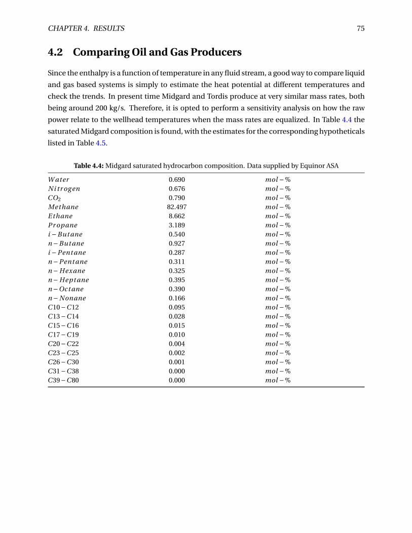
CHAPTER 4. RESULTS 75
4.2 Comparing Oil and Gas Producers
Since the enthalpy is a function of temperature in any fluid stream, a good way to compare liquid
and gas based systems is simply to estimate the heat potential at different temperatures and
check the trends. In present time Midgard and Tordis produce at very similar mass rates, both
being around 200 kg/s. Therefore, it is opted to perform a sensitivity analysis on how the raw
power relate to the wellhead temperatures when the mass rates are equalized. In Table 4.4 the
saturated Midgard composition is found, with the estimates for the corresponding hypotheticals
listed in Table 4.5.
Table 4.4: Midgard saturated hydrocarbon composition. Data supplied by Equinor ASA
W ater 0.690 mol −%Ni tr og en 0.676 mol −%CO2 0.790 mol −%Methane 82.497 mol −%Ethane 8.662 mol −%Pr opane 3.189 mol −%i −But ane 0.540 mol −%n −But ane 0.927 mol −%i −Pent ane 0.287 mol −%n −Pent ane 0.311 mol −%n −Hexane 0.325 mol −%n −Hept ane 0.395 mol −%n −Oct ane 0.390 mol −%n −Nonane 0.166 mol −%C 10−C 12 0.095 mol −%C 13−C 14 0.028 mol −%C 15−C 16 0.015 mol −%C 17−C 19 0.010 mol −%C 20−C 22 0.004 mol −%C 23−C 25 0.002 mol −%C 26−C 30 0.001 mol −%C 31−C 38 0.000 mol −%C 39−C 80 0.000 mol −%

CHAPTER 4. RESULTS 76
Table 4.5: Midgard hypothetical components properties estimated in Aspen HYSYS based on molecularweight and density.
Critical Properties
Molecular Density Normal Temper- Pressure Volume Acent-Hypothetical Weight [kg/m3] Boiling Pt [◦C] ature [◦C] [kPa] [m3/kgmole] ricity
C10-C12 178.97 145.81 804.81 372.84 25.17 0.542 0.394C13-C14 221.77 181.33 825.07 415.27 22.03 0.643 0.472C15-C16 259.99 212.28 837.70 450.32 19.32 0.750 0.550C17-C19 299.66 248.14 849.90 485.35 16.90 0.874 0.638C20-C22 341.08 289.22 863.84 521.48 14.82 1.010 0.733C23-C25 379.05 330.34 875.51 553.55 13.14 1.145 0.827C26-C30 425.45 384.70 888.61 591.66 11.35 1.323 0.950C31-C38 493.29 471.16 906.10 645.88 9.164 1.604 1.144C39-C80 628.75 662.46 936.20 751.22 5.947 2.223 1.566
Figure 4.5: HYSYS snapshot of simple cooler model used to calculate raw power potential.

CHAPTER 4. RESULTS 77
Raw Power Potential dependence of WHT
Figure 4.6 show how the raw potential from Tordis wellstream and regular water increases lin-
early with increased wellhead temperature. The Midgard discovery at the Åsgard field produces
with very high vapor fraction and it is seen that its raw potential is not directly proportional to
WHT. The data is generated from simulating the wellstreams in Aspen HYSYS as a simple cool-
ing system with 3 bara pressure drop tube side, and show that the Tordis raw thermal potential
is around 44 MW at 75◦C WHT (at the specified outlet temperature) while Midgard only has
around 30 MW. A snapshot of the HYSYS portion of the model used to generate the curves is
shown in Figure 4.5
50 60 70 80 90 100 110 120
20
30
40
50
60
70
80
·103
WHT [◦C]
Pow
er[k
W]
Pure WaterTordis FluidMidgard Fluid
Figure 4.6: Raw power potential versus cycle inlet temperature when outlet temperature is fixed at 20◦Cand total production kept at 192.5 kg/s for all cases.
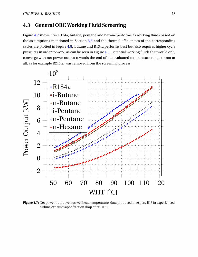
CHAPTER 4. RESULTS 78
4.3 General ORC Working Fluid Screening
Figure 4.7 shows how R134a, butane, pentane and hexane performs as working fluids based on
the assumptions mentioned in Section 3.3 and the thermal efficiencies of the corresponding
cycles are plotted in Figure 4.8. Butane and R134a performs best but also requires higher cycle
pressures in order to work, as can be seen in Figure 4.9. Potential working fluids that would only
converge with net power output towards the end of the evaluated temperature range or not at
all, as for example R245fa, was removed from the screening process.
50 60 70 80 90 100 110 120
−2
0
2
4
6
8
10
12·103
WHT [◦C]
Pow
erO
utp
ut[
kW]
R134ai-Butanen-Butanei-Pentanen-Pentanen-Hexane
Figure 4.7: Net power output versus wellhead temperature, data produced in Aspen. R134a experiencedturbine exhaust vapor fraction drop after 105◦C.
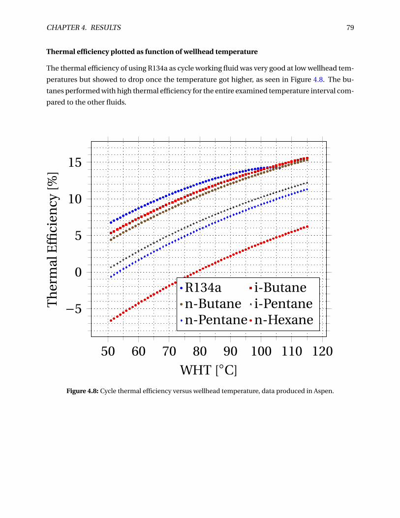
CHAPTER 4. RESULTS 79
Thermal efficiency plotted as function of wellhead temperature
The thermal efficiency of using R134a as cycle working fluid was very good at low wellhead tem-
peratures but showed to drop once the temperature got higher, as seen in Figure 4.8. The bu-
tanes performed with high thermal efficiency for the entire examined temperature interval com-
pared to the other fluids.
50 60 70 80 90 100 110 120
−5
0
5
10
15
WHT [◦C]
Th
erm
alE
ffici
ency
[%]
R134a i-Butanen-Butane i-Pentanen-Pentane n-Hexane
Figure 4.8: Cycle thermal efficiency versus wellhead temperature, data produced in Aspen.

CHAPTER 4. RESULTS 80
Expander inlet pressure plotted as function of wellhead temperature
When simulating cycles using heavier working fluids it was found that for these fluids less pres-
sure at expander inlet is possible since a large pressure ratio across the turbine would eventually
lead to condensation inside the expander. The effect is clearly seen in Figure 4.9 with butanes
and pentanes pressures being hugely different when reacting to the same cycle constraints.
50 60 70 80 90 100 110 120
0
10
20
30
40
WHT [◦C]
Pre
ssu
re[b
ara]
R134ai-Butanen-Butanei-Pentanen-Pentanen-Hexane
Figure 4.9: Expander inlet pressure versus wellhead temperature, data produced in Aspen.

CHAPTER 4. RESULTS 81
4.4 Subsea ORC Working Fluid Screening
A subsea cycle operates under higher natural pressure than other cycles due to the sea water
level. This means that the working fluids that are usually proposed for low temperature organic
Rankine cycles may not be suitable for operation, and that the potential for using lighter fluids
should be evaluated. It is also clear that selecting a fluid with low environmental risk is very
important, since a leak of the working fluid would directly pollute the ocean. Therefore, we opt
to evaluate light natural gases that are naturally present in the Tordis reservoir composition as
working fluids, since they are most easily accessible and involve less environmental harm po-
tential. Figure 4.10 shows phase curves for the fluids methane, ethane, propane, iso-butane and
CO2. Extra tick marks has been added to show where the cycle is expected to operate, especially
important since a subsea design is more constrained pressure wise than one topside. The nat-
ural pressure at 250 meters depth is around 26 bars. The first observation from Figure 4.10 is
that methane tends to stay in gaseous state for the entire operating range, and is therefore not
well suited for application in a sub-critical cycle. CO2 and ethane are in gaseous state at natu-
ral pressure and 14◦C, but can be compressed into liquid state by adding relatively few bars of
pressure. Propane is in liquid state at this temperature with a large pressure margin and stays
liquid when heated to 70◦C at natural pressure. Iso-butane is even less suited for operation than
propane because of its tendency to stay liquid for the entire operating range.
Since it is observed that CO2 and ethane are plausible choices as working fluids which both
require a highly pressurized system, a simulation has been run to see the effect of changing the
expander inlet pressure on net output potential. Figure 4.11 shows the simulation results and
it should be noted that a basic ORC system model was used for this analysis as well. From the
curves it is evident that while CO2 has a slightly higher net power output peak, it requires 40 bar
higher expander inlet pressure to achieve it. Ethane is therefore determined as the fluid with the
best suited properties for ORC application in this pressure and temperature range, but since it
is not perfectly suited a slight adaption of the working fluid is proposed. Figure 4.13 show phase
curves of ethane, propane and a binary mix of these two hydrocarbons. By experimenting in
Aspen it was found that adding 18 mol-% of propane to ethane would yield a binary fluid that
requires much less added pressure to condense compared to pure ethane. In addition, the re-
sulting fluid has its critical point only at a slightly higher temperature and would still allow the
binary mixture to stay in gaseous state at very high pressures when the working temperature is
70◦C.
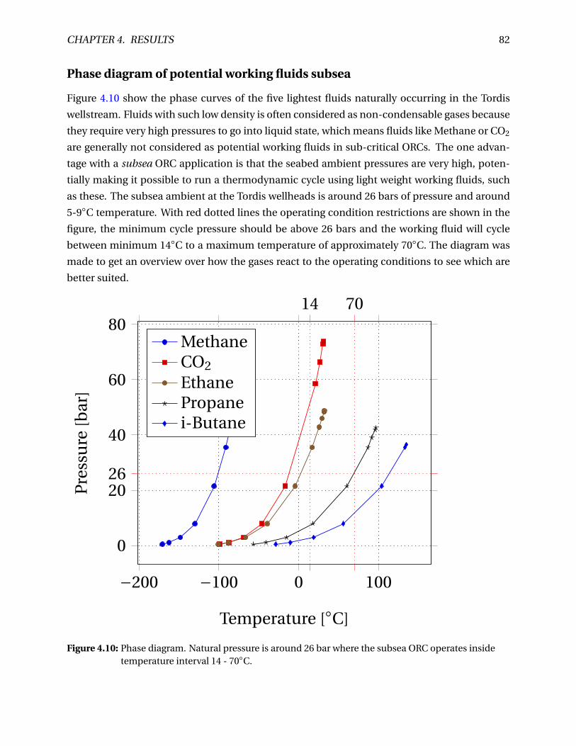
CHAPTER 4. RESULTS 82
Phase diagram of potential working fluids subsea
Figure 4.10 show the phase curves of the five lightest fluids naturally occurring in the Tordis
wellstream. Fluids with such low density is often considered as non-condensable gases because
they require very high pressures to go into liquid state, which means fluids like Methane or CO2
are generally not considered as potential working fluids in sub-critical ORCs. The one advan-
tage with a subsea ORC application is that the seabed ambient pressures are very high, poten-
tially making it possible to run a thermodynamic cycle using light weight working fluids, such
as these. The subsea ambient at the Tordis wellheads is around 26 bars of pressure and around
5-9◦C temperature. With red dotted lines the operating condition restrictions are shown in the
figure, the minimum cycle pressure should be above 26 bars and the working fluid will cycle
between minimum 14◦C to a maximum temperature of approximately 70◦C. The diagram was
made to get an overview over how the gases react to the operating conditions to see which are
better suited.
−200 −100 0 100
0
20
40
60
8014 70
26
Temperature [◦C]
Pre
ssu
re[b
ar]
MethaneCO2
EthanePropanei-Butane
Figure 4.10: Phase diagram. Natural pressure is around 26 bar where the subsea ORC operates insidetemperature interval 14 - 70◦C.

CHAPTER 4. RESULTS 83
Expander inlet pressure effect on performance sensitivity plot
Figure 4.11 show how increasing the cycle maximum pressure, which correspond to the ex-
pander inlet pressure, affects the calculation of net power output from the unit. The analysis
was performed for two different working fluids, ethane and CO2, and the script given in Ap-
pendix B.1.4 was used to iterate through all the pressure states. Both fluids peak at around 3
MW net power output, with CO2 giving a slightly higher output at the expense of requiring 40
bars higher cycle maximum pressure. The figure underpins how the choice of working fluid
directly affects the selection of other ORC components. For example, using CO2 will require a
more powerful pump that can boost the working fluid from the ambient to 111 bars, while using
ethane would require a lesser rated pump for boosting to 71 bars.
40 60 80 100 120 140 160
0
1
2
3
·103 71 111
Expander Inlet Pressure [bar]
Net
Pow
er[k
W]
EthaneCO2
Figure 4.11: Effect of increasing the highest cycle pressure point. After peak liquid droplets are seen inthe expander outlet.
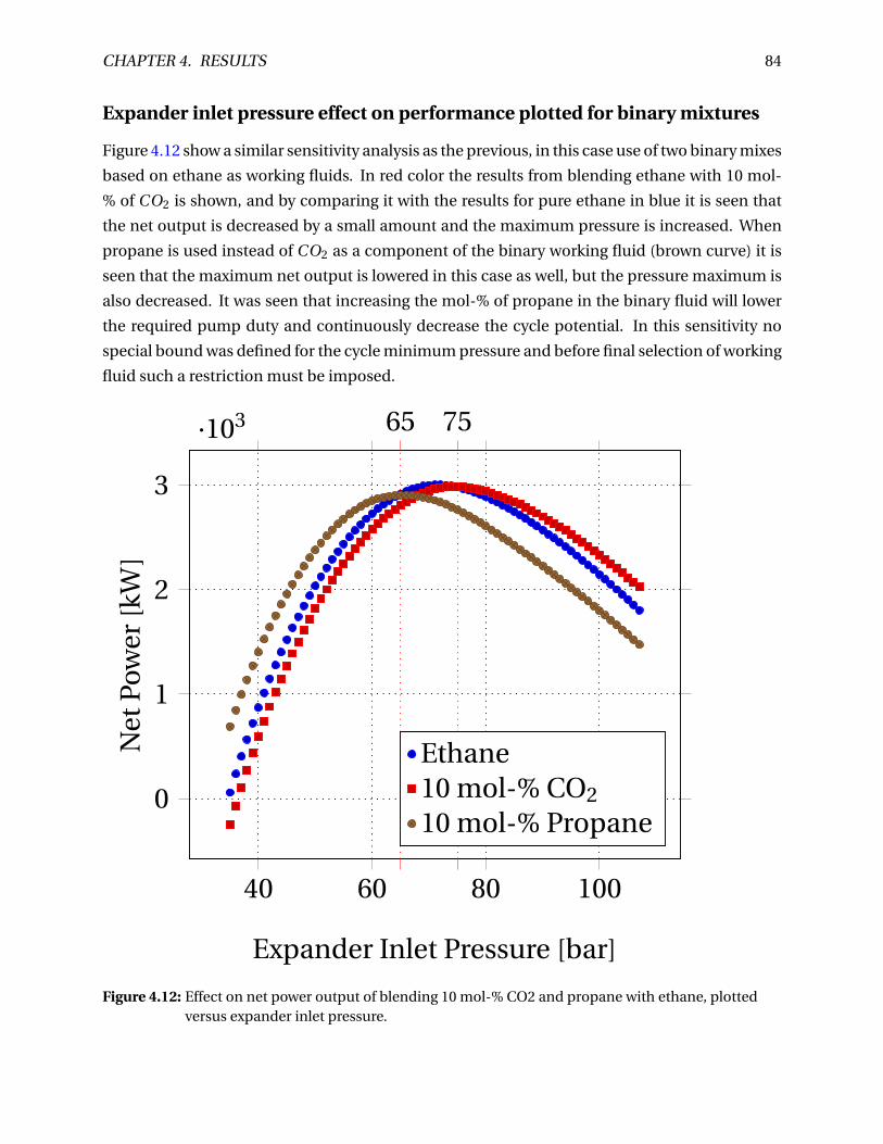
CHAPTER 4. RESULTS 84
Expander inlet pressure effect on performance plotted for binary mixtures
Figure 4.12 show a similar sensitivity analysis as the previous, in this case use of two binary mixes
based on ethane as working fluids. In red color the results from blending ethane with 10 mol-
% of CO2 is shown, and by comparing it with the results for pure ethane in blue it is seen that
the net output is decreased by a small amount and the maximum pressure is increased. When
propane is used instead of CO2 as a component of the binary working fluid (brown curve) it is
seen that the maximum net output is lowered in this case as well, but the pressure maximum is
also decreased. It was seen that increasing the mol-% of propane in the binary fluid will lower
the required pump duty and continuously decrease the cycle potential. In this sensitivity no
special bound was defined for the cycle minimum pressure and before final selection of working
fluid such a restriction must be imposed.
40 60 80 100
0
1
2
3
·103 65 75
Expander Inlet Pressure [bar]
Net
Pow
er[k
W]
Ethane10 mol-% CO2
10 mol-% Propane
Figure 4.12: Effect on net power output of blending 10 mol-% CO2 and propane with ethane, plottedversus expander inlet pressure.

CHAPTER 4. RESULTS 85
Bubble- and dew point lines of binary working fluid mixture
Figure 4.13 is a PT-phase diagram where the phase curves of ethane, propane and a binary mix
of the two is plotted. The composition of the binary fluid is 82 mol-% ethane and 18 mol-%
propane, and it can be seen that this composition has the bubble point line cross through the
point of 26 bar and 14◦C. This means that if the cycle minimum pressure at condenser outlet has
these conditions, the working fluid will be in a saturated liquid state. When selecting the final
working fluid for the subsea cycle it is therefore recommended to use a binary mix with max-
imum 18 mol-% propane, as any higher amount would inconvenience the condensation and
evaporation processes. For example, look to the phase curve for pure propane. Here it is seen
that at 14◦C the fluid is in liquid state at subsea ambient pressures and it barely starts to evapo-
rate when the temperature is increased to 70◦C. Considering that the pressure level is boosted at
evaporator outlet, the fluid needs to display a steeper curve within the cycle operating interval.
It should be noted that using less than 18 mol-% propane will imply a higher minimum pressure
in the cycle in order to condense the working fluid to zero vapor fraction before it is boosted
through the centrifugal pump.
−100 −50 0 50 100
0
20
40
14 70
26
Temperature [◦C]
Pre
ssu
re[b
ar]
EthaneBinary WF BPBinary WF DPPropane
Figure 4.13: Phase diagram. 18 mol-% propane mixed with ethane.

CHAPTER 4. RESULTS 86
4.5 Subsea ORC Operating Conditions
Pw f −2, Tw f −2
Ptur b
mw f , Pw f −1, Tw f −1
Pw f −3, Tw f −3
Pw f −4, Tw f −4
Ppump
Ph f −2, Th f −2
mh f , Ph f −1, Th f −1
Figure 4.14: The operating conditions of the evaluated subsea binary cycle are listed in Table 4.6.
According to Toffolo et al. (2014) an ORC should be modeled based on the following four key
decision parameters. The maximum pressure of the cycle, the flow rate of the working fluid,
degree of superheat and condensation pressure. An ORC placed subsea will however be even
more restricted in many ways, the cycle minimum pressure would for example be especially im-
portant. It were necessary to perform the design of an optimal cycle working condition based
on the literal bounds of the Tordis wellstream in combination with some realistic assumptions
and limitations. The design has to address the following two main concerns. The first concern
is that the wellstream represents a low enthalpy heat source due to its relatively low WH tem-
perature and mass rate, meaning heat has to be efficiently transferred to the cycle working fluid

CHAPTER 4. RESULTS 87
Table 4.6: Operating conditions for a ORC configuration as shown in Figure 4.14 based on the selectedbinary working fluid and subsea pressure and temperature conditions.
Parameter Operating condition [Unit]
Working fluid mass flowrate, mw f 81.0 [kg/s]Expander inlet pressure, Pw f −1 63.8 [bar]Expander inlet temperature, Tw f −1 70.8 [◦C]Expander outlet pressure, Pw f −2 31.0 [bar]Expander outlet temperature, Tw f −2 22.0 [◦C]Cooling manifold outlet pressure, Pw f −3 30.0 [bar]Cooling manifold outlet temperature, Tw f −3 14.4 [◦C]Pump outlet pressure, Pw f −4 65.0 [bar]Pump outlet temperature, Tw f −4 21.7 [◦C]Wellstream mass flowrate, mh f 192.5 [kg/s]Wellstream inlet pressure, Ph f −1 40.0 [bar]Wellstream inlet temperature, Th f −1 75.0 [◦C]Wellstream outlet pressure, Ph f −2 37.4 [bar]Wellstream outlet temperature, Th f −1 44.7 [◦C]
unless production is significantly increased. The second big concern that limits the cycle design
freedom of choice is that the pressures subsea are very high, effectively limiting the amount
of attractive working fluid substances. As mentioned in the annotated bibliography section of
this thesis, Saleh et al. (2007) calculated thermal efficiency for a large range of working fluids
suited for low temperature cycles and it was shown that the benefit of having an internal heat
exchanger was usually 1% or less. For this reason, it were not opted to use IHE for this cycle
evaluation as the added benefit is relatively modest. Earlier in this thesis the wellstream heat
potential has been evaluated using an arbitrary value of ∆T = 50◦C, but at this point it were
necessary to calculate the potential heat transfer using a real shell and tube heat exchanger and
the chosen working fluid. In the PT-diagram in Figure 4.13 it were shown how the bubble point
line of a ethane and 18 mol% propane crosses the 26 bar and 14 ◦C point, meaning this blend
could run a cycle with natural pressure as minimum pressure and 5◦C cooling pitch. It is not
optimal to be restrained to having natural pressure as minimum pressure, therefore a binary
working fluid of ethane and 10 mol% propane were used for actual cycle calculation, because it
allows for a higher cycle pressure minimum by a slight shift of the fluid mix phase curve. The
binary fluid composition and the Tordis wellstream conditions were used as input for the evap-
orator shell and tube heat exchanger calculation, and a realistic heat transfer of 23.3 MW were
estimated. This heat exchange put the wellstream outlet temperature to 44.78 ◦C, meaning a
real ∆T = 75−44.78 = 30.22◦C. The evaporator heat exchanger calculation is summarized with
results in Section 4.7. In order to maximize the thermal efficiency of the cycle it were opted to

CHAPTER 4. RESULTS 88
use a passive cooling manifold to avoid the duty that having an extra pump for a S&T cooler
would require. The passive cooling system would be required to transfer 21.8 MW worth of heat,
effectively condensing working fluid gas at 22◦C to sub-cooled liquid at 14.45 ◦C. The efficien-
cies related to individual equipment were defined based on common assumptions used when
ORCs are modeled. It is common to use a turbine with 85% isentropic efficiency, and a pump
operating at 80% isentropic efficiency. The mechanical efficiency of turbine is expected to be
very high and is therefore kept at 100% in this analysis. Additional common assumptions are
also to model the ORC with superheating, subcooling and pinch point approximately equal to
5◦C and less than 1 bar shell-side pressure drops in the heat exchangers, and these premises
are true also for the model presented here. Table 4.6 lists a summary of the chosen operating
conditions, but it should be noted that a slightly more efficient cycle is possible by reducing the
minimum pressure level from 30 bars towards natural pressure because a lesser duty would be
required from the pump.
4.6 Design Standards and Cycle Control Requirements
In a real application of a subsea ORC the operating conditions will not be steady state, which
means that the cycle has to have a system for both supervision and control, which as a main
purpose is used to ensure that the production of electricity is maximized at all times. This sec-
tion lists the main controllers in addition to PT-gauges which are necessary from an output op-
timization perspective and also informs on relevant physical requirements based on the Process
system design NORSOK standard. This review over the different necessary control elements is
split into two subsections, shell and tube heat exchangers in the first and rotating equipment in
the other.
4.6.1 Subsea Heat Exchangers
The content in that follows will be based on the NORSOK P-002 (2014) requirements for heaters
and coolers operating on the NCS. The shell and tube heat exchangers should be designed so
that both sides can withstand the maximum design temperature, it should also be ensured that
the temperature is kept at a level where hydrates and wax does not deposit. As an example, this
means that the tube side of the cooler in a subsea ORC should at least be rated for the temper-
ature of the working fluid at shell-side inlet and vice versa. If the heat exchanger is in an oil
train, such as the evaporator in the ORC is, it is required that it is designed with all realistic flow
rates and temperatures in mind. Once the heat exchanger area is determined it should be added
excess area to the design to account for fouling, which is referred to as design margin. The re-
quirement for the design margin is different in every case, and recommendations can be found

CHAPTER 4. RESULTS 89
at The Tubular Exchanger Manufacturers Association, Inc. (TEMA) for specific applications. In
cases where it is opted to use a different type of heat exchanger the engineers are referred to
NORSOK R-002 for recommendations. It is also required that nozzles are installed onto or in
close proximity to the heat exchanger, so that it can be flushed with chemicals for cleaning pur-
poses. A check valve or shut down valve can be installed upstream the S&T exchanger in case of
leakage or some kind of internal rupture, this is to minimize chances for contamination through
back flow into the side of lowest pressure. In cases where the shell side fluid is cycled with a very
high rate it is a possibility for vibration of the tubes inside the shell, therefore it must be taken
into account in the exchanger design that such vibrations shall not occur to the extent where
the apparatus may be damaged. When it comes to thermal optimization, a main actuator of the
cycle is a bypass valve that will be used to control the vapor fraction entering the evaporator.
The Tordis field produces a small amount of gas which is contained in the wellstream that is
channelled tube side with the oil in the evaporator. The bypass valve can then be used to let
a certain amount of gas and possibly condensate to be routed past the evaporator system, and
that way the engineers can control the evaporator pressure with high accuracy.
4.6.2 Subsea Pump and Turbine
The NORSOK standard does not include many special requirements for submerged pumps or
turbines in general, it is mainly the engineers job to select units that are rated for the realistic op-
erating conditions. For sub-cooled liquids and in relation to the discharge flow lines it is stated
that the pipe dimension should be designed with the centrifugal pump in mind, such that the
pressure drop will be a maximum of 0.25 bar per 100 meters of line. If a reciprocating pump is
used, the flow line sizing should be determined based on recommendations by ISO 13703. When
it comes to the thermal optimization of the ORC, the pump functions as another main actuator
because working fluid mass rate entering the evaporator can be directly controlled through the
pump speed. In practice this means that the pump is key for controlling the temperature (de-
gree of superheat) at evaporator outlet and expander inlet. A thing to think about when doing
the turbine design is to consider if the produced electricity from the ORC should match the Nor-
wegian power socket. Since the standard voltage in Norway is 230 V and the standard frequency
is 50 Hz this means that the rotational speed of the rotor has to be 3000 rounds per minute. It
might therefore be necessary to use a gear box to equalize the speed of the generator with grid
frequency. The turbine speed also has a direct effect on the energy contained in the fluid at ex-
pander outlet, and can therefore serve as another control element for cycle optimization. A final
main actuator for the subsea ORC is made by installation of a by-pass valve around the turbine,
which is mainly there as a safety measure. During normal cycle operation this by-pass will be
closed for flow, and it is only opened in the event where working fluid condensate is registered
in the expander. The by-pass valves were added to the illustration of the subsea ORC which now
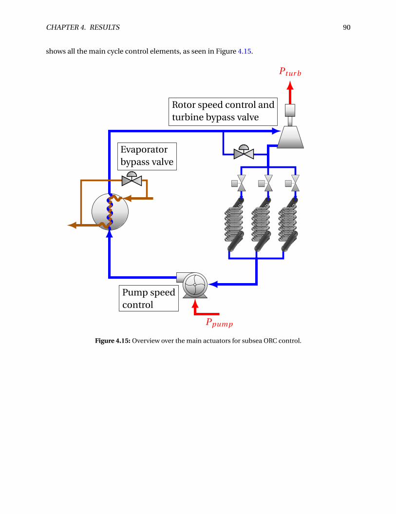
CHAPTER 4. RESULTS 90
shows all the main cycle control elements, as seen in Figure 4.15.
Ptur b
Rotor speed control andturbine bypass valve
Ppump
Pump speedcontrol
Evaporatorbypass valve
Figure 4.15: Overview over the main actuators for subsea ORC control.

CHAPTER 4. RESULTS 91
4.7 Approximate Component Sizes
In order to get an idea of the necessary sizing for an ORC installed at Tordis, a rough pre-design
has been made based on a subsea model. Special emphasis has been made on the design of
the heating system. Note that the numbers presented for evaporator cost should be regarded as
ballpark numbers which are mostly suited for financial comparison of different design options.
4.7.1 Subsea ORC Component Sizing
Results from the early evaluation of component sizes for the Tordis subsea ORC model are sum-
marized below. Calculations have been performed based on a binary working fluid consisting of
10 mol-% propane blended with ethane. Table 4.7 show input data for the calculations based on
using basic a ORC configuration without internal heat exchanger which has been fitted to have
as high net power output as possible while operating as a subcritical cycle.
Table 4.7: Input data used for component size calculations made in Section 4.7.1 with a binary blend ofethane and propane as working fluid using a basic ORC configuration.
Parameter Simulated Value [Unit]
Working fluid type Binary [-]Working fluid mass flowrate 81.0 [kg/s]Expander inlet pressure 63.8 [bar]Expander outlet pressure 31.0 [bar]Expander effciency 85.0 [%]Expander mechanical efficiency 100.0 [%]Gross power output 2384.0 [kW]Pump duty 283.1 [kW]Pump efficiency 80.0 [%]Geothermal fluid mass flowrate 192.5 [kg/s]Geothermal fluid temperature 75.0 [◦C]Geothermal fl. exit temperature 44.78 [◦C]Net plant power 2100.9 [kW]Thermal efficiency 9.034 [%]
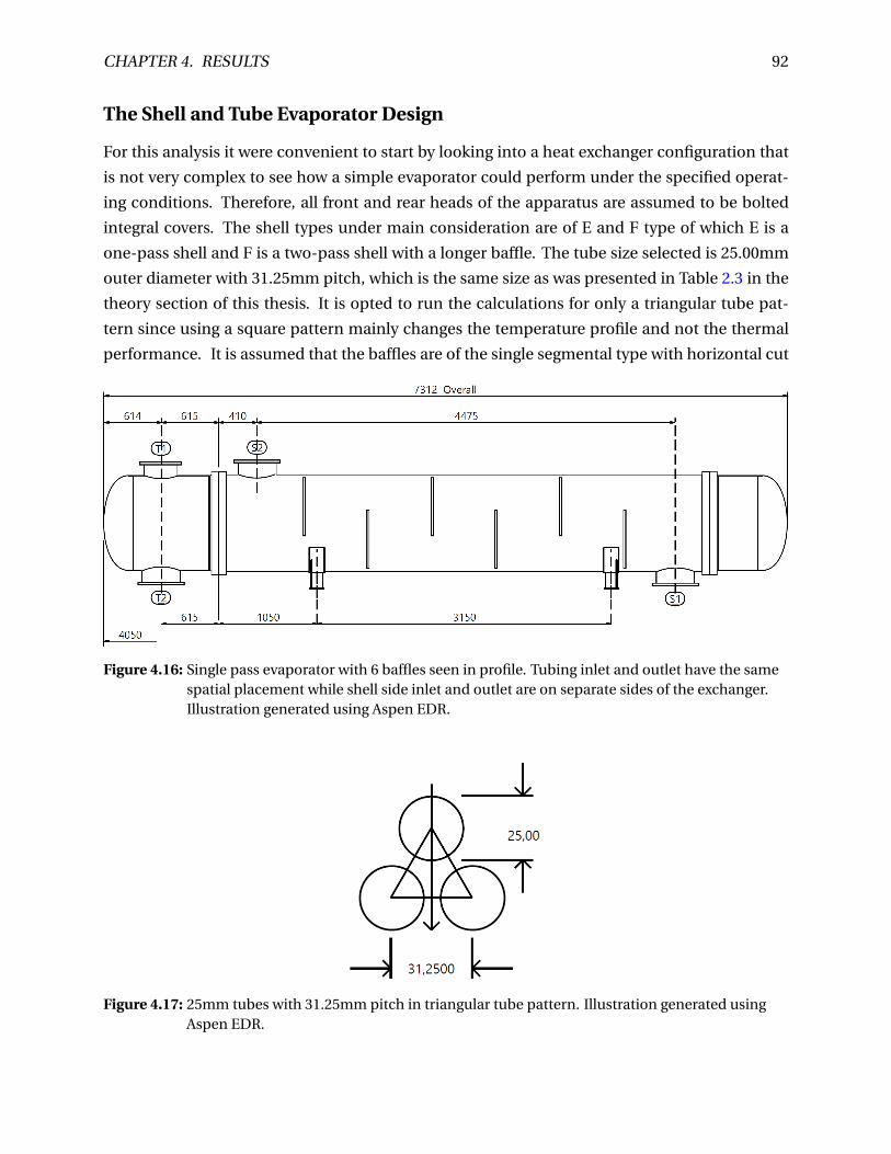
CHAPTER 4. RESULTS 92
The Shell and Tube Evaporator Design
For this analysis it were convenient to start by looking into a heat exchanger configuration that
is not very complex to see how a simple evaporator could perform under the specified operat-
ing conditions. Therefore, all front and rear heads of the apparatus are assumed to be bolted
integral covers. The shell types under main consideration are of E and F type of which E is a
one-pass shell and F is a two-pass shell with a longer baffle. The tube size selected is 25.00mm
outer diameter with 31.25mm pitch, which is the same size as was presented in Table 2.3 in the
theory section of this thesis. It is opted to run the calculations for only a triangular tube pat-
tern since using a square pattern mainly changes the temperature profile and not the thermal
performance. It is assumed that the baffles are of the single segmental type with horizontal cut
Figure 4.16: Single pass evaporator with 6 baffles seen in profile. Tubing inlet and outlet have the samespatial placement while shell side inlet and outlet are on separate sides of the exchanger.Illustration generated using Aspen EDR.
Figure 4.17: 25mm tubes with 31.25mm pitch in triangular tube pattern. Illustration generated usingAspen EDR.

CHAPTER 4. RESULTS 93
Table 4.8: Assumptions made as the evaporator design basis.
Parameter Assumption [Unit]
TEMA Type: BEMTube OD: 25.00 [mm]Tube pitch: 31.25 [mm]Tube Pattern: 30-TriangularTubes in baffle window: YesBaffle Type: Single sementalBaffle cut orientation: HorizontalExchanger material: Carbon Steel
Table 4.9: Proposed design based on assumptions made in Table 4.8 and thermal requirements.
Parameter Proposed size: [Unit]
Shell ID: 975.0 [mm]Shell OD: 1045.0 [mm]Tube length: 5250.0 [mm]Baffle spacing center: 685.0 [mm]Number of baffles: 6 [-]Number of tubes: 700 [-]Number of passes 2 [-]Shells in Series 5 [-]Shells in parallel 1 [-]Excess surface: 0 [%]
orientation, that the fouling resistance is zero as design margin can be added at later on, and that
the heat exchanger material used is carbon steel. An evaporator with E type shell is proposed
as seen in Figure 4.16. The tubes are installed using the triangular tube pattern shown in Figure
4.17 and the full crossectional geometry can be seen in Appendix C.1. All the main technical
assumptions made for the design is listed in Table 4.8 and Table 4.9 contain a summary of key
results for the proposed exchanger geometry. Using five shells of approximately 6-meter length
in series will cover the required heat transfer by installing a calculated number of 700 tubes
and 6 baffles in each. This evaporator design has no estimated excess surface, which means
any fouling will affect the thermal efficiency of the system. The temperature development spa-
tially can be seen graphically from the temperature profiles plotted in Figure 4.18. As previously
mentioned, the front and rear heads are assumed to be very simple in order to get the cheapest
possible solution. Table 4.10 show expected prices based on the Aspen cost correlation along
with a system mass estimate. The thermal performance of this design is listed in Table 4.11 and
the total heat exchange were shown to be 23260.7 kW with an effective area of 1397.8 m2.

CHAPTER 4. RESULTS 94
Table 4.10: Approximate evaporator weight and cost using carbon steel as building material.
Weights [kg] Cost approximation [USD]
Shell 5816.2 Labor 343 734Front head 1814.3 Tube material 59 655Rear head 1288.5 Other material 143 404Bundle 5764.2
Total weight - Empty 14683.0 Total (one shell) 109 359Total weight - Water filled 19149.9 Total (all shells) 546 795
Table 4.11: Summary of thermal performance related to the proposed evaporator using a binaryworking fluid.
Shell Side Tube Side
Parameter In Out In Out [Unit]
Vapor mass flow rate 0 81.0 2.49 2.10 [kg/s]Liquid mass flow rate 81.0 0 190.01 190.4 [kg/s]Vapor mass quallity 0 1 0.01 0.01 [-]Temperature 21.67 70.73 75.00 44.78 [°C]Pressure 65.0 63.76 40.0 37.40 [bar]
Film coefficient 3722.2 3936.4 [W/(m²-K)]Fouling resistance 0 0 [m²-K/W]Pressure drop 1.237 2.601 [bar]
Total heat exchanged 23260.7 [kW]Effective area 1397.8 [m²]Effective mean temp. difference 9.45 [°C]

CHAPTER 4. RESULTS 95
Temperature plotted as function of evaporator axial length
The expected temperature development of the working fluid and the Tordis wellstream in the
heating system can be seen in Figure 4.18. The reason behind the "bend" on each wellstream
segment in red is that the tube side inlets and outlets are on the same side of the shells, because
the heaters are designed as dual pass exchangers.
0 5 10 15 20 25 30
20
40
60
80
Tube length (shells in series) [m]
Tem
per
atu
re[◦
C]
Binary fluidWellstream
Figure 4.18: Temperature profile inside the evaporator system with shells as shown in Figure 4.16 withtriangular tube pattern. Tubing inlet and outlet have the same spatial placement while shellside inlet and outlet are on separate sides of the exchanger.
CHAPTER 4. RESULTS 96
Cooling System Selection
The working fluid is in gaseous state at 21.99◦C and 31 bars at the expander outlet. Cooling the
working fluid down to a condensed state at this pressure level and current rate requires a heat
transfer of 21826.37 kW , effectively putting the working fluid down to 14.45◦C at the cooling
system outlet. Using an active cooling system such as a shell and tube heat exchanger is an op-
tion, but it would imply an extra duty on the system due to pumping of the coolant brine. To
maximize the power output, it would seem convenient to use a passive subsea cooling system
instead that utilizes the natural convection effect seen subsea.
In Section 2.3.3 the concept of using a sectioned passive cooler manifold was introduced with
a short description. One of the companies providing this technology is Future Technology AS
and they use their in-house software SIMCOOL as a design tool to scale their exchangers to
proper sizing. Table 4.12 show the technical specification and limitations of the design and
judging from the list it is clear that the passive sectioned exchanger would cover the needs of
the proposed cycle. The size of the structure can not be estimated precisely at this point, but it
is known that sectioned passive heat exchangers are roughly four times the size of a tube and
heat exchanger with the same inlet and outlet conditions.
It is possible to make rough size approximations based on the passive cooler model presented
in Section 3.5. Since the required amount of heat transfer is known in this case, the calculations
can be simplified greatly if it is assumed that the inner and outer pipe walls have the same tem-
perature as their respective mediums. The biggest reason for making the simplification is the
fact that our passive cooler condenses the working fluid, which means the Kern heat transfer
equations for condensation processes would have to be used in addition to the standard mod-
elling of the sub-cooling of liquid. Because of this effect, it is opted to only calculate the amount
of outer pipe area required for the super duplex solid to conduct the 21826.37 kW of heat and
completely disregard the natural and forced convection that takes place in reality, effectively cal-
culating the minimum value for required area. Using the thermal properties of the duplex alloy
2507 UNS S32750 and assuming outer pipe radius of 0.025m with 0.005m thickness for the coils,
it was found that necessary outer pipe surface area is 949.9 m2. This was done by calculating the
pipe length with Equation (4.1) then multiplication with the pipe circumference based on the
assumed pipe radius as in Equation (4.2). Approximate minimum cooler weight is calculated in
similar manner, using Equation (4.3) for empty system and Equation (4.4) for system filled with
condensate. The density of the super duplex and the working fluid condensate is respectively
7750 kg /m3 and 385.1 kg /m3, which means the weight of an empty system is 33.12 tonnes and
condensate filled system is 36 tonnes.

CHAPTER 4. RESULTS 97
Table 4.12: Technical specification of available passive cooler compared with thermal requirements ofthe proposed subsea thermodynamic cycle.
Technical specification Limitations Subsea cycle
Process inlet temperature Up to 150◦C 21.99◦CCooling rate Up to 50 MW 22 MWPressure drop In accordance to client request 1 barOperating depth Down to 2000m 250m
Scalability HighControllability 5%-100%Material Pipes are super duplexDimensions and weight Depends on req. cooling rateControl valve AxialSensors 3 Dual P&T sensorsDesign life >25 years
Lpi pe = Q ln(ro/ri )
2πκSD (Ti −To)(4.1)
Api pe =2πro ×Lpi pe (4.2)
mpi pe, e =ρSDπ(r 2o − r 2
i )×Lpi pe (4.3)
mpi pe, f =mpi pe, e +ρw f πr 2i ×Lpi pe (4.4)

CHAPTER 4. RESULTS 98
Basic design features of the turbine
Since thermodynamic software has been used in the ORC modeling, the energy analysis consid-
eration is done using the computer. However, the resulting parameters from the Aspen HYSYS
estimation can be used to get an idea of the basic design features of the rotating equipment.
By basic design features of a turbine it is pointed to physical dimensions of the unit, required
blade angles and velocity ratios of all its stages. The gas turbine can be of radial or axial type,
and in this assessment it is assumed that a turbine of the axial type is selected for the subsea
ORC. Referring back to the theory related to the velocity diagrams of a two-stage turbine shown
in Figure 2.10, the ideal design features of an unit can be determined using the mass rate and
energy state of the ORC cycle working fluid along with well-known geometric relationships.
Figure 4.19 represents the control volume used for the assessment, where mass rate and en-
thalpy states of the working fluid at turbine inlet and outlet is known. In this case the numerical
value for enthalpy is taken directly from the thermodynamic modelling software, but it could
also have been determined using a Mollier diagram and the PT conditions on either side of the
unit, if the working fluid were not of binary type. It were mentioned earlier in this thesis that it
is possible to design a turbine using a velocity compounding technique where the entire pres-
sure drop happens in the inlet nozzle of the turbine, and assuming the turbine is of such type
makes the thermodynamic analysis easier as only one working fluid expansion stage needs to
be considered. Note that Ptur b is gross power and not the cycle net power output. It is opted to
perform the analysis by assuming that the working fluid expansion in the nozzle is an isentropic
process and that the gross power output requirement corresponds to a isentropic efficiency at
85%. When the nozzle expansion is isentropic it essentially means that there is no friction and
the working fluid entropy will be unchanged. The enthalpy after isentropic expansion of the bi-
nary working fluid (at nozzle outlet) is estimated to hw f −2 = −2855 kJ/kg by the software. This
makes calculating the necessary inlet diameter of the turbine a trivial task, and we assume ve-
locity compounding using two stages, just as was derived in the theory section of this thesis.
mw f = 81kg /s, hw f −2 =−2855k J/kg
Ptur b = 2366kW
mw f = 81kg /s, hw f −1 =−2821k J/kg
Figure 4.19: Control volume for thermodynamic analysis of the proposed subsea ORC turbine withisentropic pressure expansion.

CHAPTER 4. RESULTS 99
Finding the inlet velocity of the working fluid can be done by using the energy equilibrium
across the nozzle. It were explained in Section 2.3.1 that a certain amount of the energy po-
tential exits the turbine outlet as kinetic energy proportional to V 2out /2, and the same line of
thinking can be used here to solve for the inlet velocity. Since energy is conserved, the balance
can be expressed as with Equation (4.5) which states that the amount of energy before and after
expansion is the same.
hw f −1 = hw f −2 +V 2
1
2(4.5)
The equation can be solved for the working fluid velocity at the inlet V1 by rearranging the terms
as shown in Equation (4.6), please note that 1 kJ/kg = 1000 m2/s2 and that the V1 label corre-
sponds to the vector in the first stage velocity triangle diagram in Figure 4.20.
V1 =√
2hw f −1 −2hw f −2
=√
2(hw f −1 −hw f −2)
=√
2(−2821×1000 m2/s2 −−2855×1000 m2/s2)
=20p
170 m/s
=260.8 m/s
(4.6)
It was derived earlier (see Equation (2.37)) that the highest possible gross power output for a
two-stage turbine of this type would be E = 8u2, where u is the blade velocity. This result is
very useful because it allows for calculating the required radial size of the turbine at the nozzle.
Equation (4.7) relates blade velocity to turbine gross power and working fluid mass rate, and by
solving for u it is found that the blades will rotate at tip speed 65.5 m/s in the calculation shown
by Equation (4.8). After determining tip speed at the nozzle, it is possible to find the length of the
blades at the inlet. This is done in Equation (4.9), and it uses the fact that the standard electrical
grid frequency in Norway is 50 Hz, which means the rotor should revolve at 3000 rounds per
minute. It is easily shown that 3000 rounds per minute equals 314.16 radians per second, and
with that figure input in the equation it were found that the optimum radius ri at the turbine
inlet to match grid frequency is 0.19 meters.
ETot al =Ptur b
mw f
8u2 =Ptur b
mw f
(4.7)

CHAPTER 4. RESULTS 100
u =√
Ptur b
8×mw f
=√
2366×1000W
8×81 kg /s
=√
2366×1000 kg m2/s3
8×81 kg /s
=√
2366×1000 kg m2/s3
8×81 kg /s
=65p
70
9m/s
=60.4 m/s
(4.8)
Di =2× ri = 2× u
r evoluti ons
=2× 60.4 m/s
314.16 r ad/s
=2×0.19m
(4.9)
The velocity triangle method presented in Murty (2018) can be put to use for help calculating
the rest of the unknowns for both stages of the turbine. The working fluid exit velocity out the
turbine outlet can be determined using geometrical considerations of Figure 4.20, along with
figuring out what angles are most suitable for the turbine blades. The relation shown in Equa-
tion (4.10) was derived in the theory section, and is used for solving for optimum inlet nozzle
angle for maximum turbine efficiency, α1, as seen in Equation (4.11). Note that to simplify the
calculations in velocity compounding it is often assumed constant axial velocity through the
turbine stages, and that assumption is true for the calculations made here as well.
u
V1= sin(α1)
4(4.10)
α1 = arcsin4×u
V1
= arcsin(4×60.4 m/s
260.8 m/s)
=67.9◦
(4.11)
Earlier in this thesis it was shown that the maximum utilization factor for a two-stage setup such
as this could be simplified to the expression εM ax = sin2α1, which in this case would translate to

CHAPTER 4. RESULTS 101
εM ax = 0.858. This means that 14.2% of the kinetic energy potential entering the turbine will be
lost to friction, turbulence and other factors. Determining more of the required physical traits
of a unit before final turbine selection could potentially prove useful. The calculated maximum
utilization factor is of a typical order for an industrial turbine, and it is opted to determine the
rest of the related unknowns such as optimum positioning of the blades (blade angles), fluid rel-
ative velocities and the remaining nozzle angles. Referring to Figure 4.20, the assessment starts
with decomposing the first stage vectors into x- and y components in Cartesian coordinates as
seen in Equations (4.12)-(4.14). In Equation (4.15) the Pythagorean theorem is used to calculate
the absolute length of the relative velocity vector w , which is the relative velocity of the working
fluid after contact with rotor. The value is then used to calculate the blade angle β for the first
stage inlet in Equation (4.16), and it was shown that these blades should have 61.6◦ tilt.
Vy1 =V1 × sin(α1)
=260.8 m/s × sin(67.9◦)
=241.6 m/s
(4.12)
Vx1 =V1 ×cos(α1)
=260.8 m/s ×cos(67.9◦)
=98.1 m/s =Vx2
(4.13)
wy1 =Vy1 −u
=241.6 m/s −60.4 m/s
=181.4 m/s = wy2
(4.14)
w1 =√
w 2y1 +V 2
x1
=√
181.42 +98.12 m/s
=206.2 m/s
(4.15)
|β1| = arctan(wy1
Vx1)
= arctan(181.4 m/s
98.1 m/s)
=61.6◦ = |β2|
(4.16)

CHAPTER 4. RESULTS 102
First stage Second stage
Figure 4.20: Velocity triangles for first and second stages, used for explanation of the thermodynamicanalysis of the subsea ORC turbine. Figure taken from Murty (2018).
The same type of assessment is performed for the exit velocity triangle of the first stage. Using
the fact that the relative velocity vectors w1 and w2 are of same length, it is possible to deter-
mine the y-component of the exit velocity vector Vy2 as shown by Equation (4.17). Since the
axial velocity is assumed constant through all the turbine stages, finding the exit velocity V2 is a
trivial task as seen in Equation (4.18). It should be stated that even though the velocities inside
the turbine that have been calculated so far are not of particular interest by themselves, they are
still direct consequences of using a geometrical design that give the most optimum utilization
factor to minimize the energy state of the working fluid at turbine outlet. The most favorable
exit nozzle angle of stage one α2 was shown to be 51◦ by Equation (4.19).
Vy2 =wy2 −u
=181.4 m/s −60.4 m/s
=121 m/s
(4.17)
V2 =√
V 2y2 +V 2
x2
=√
1212 +98.12 m/s
=155.8 m/s
(4.18)
|α2| = arctan(Vy2
Vx2)
= arctan(121 m/s
98.1 m/s)
=51◦
(4.19)
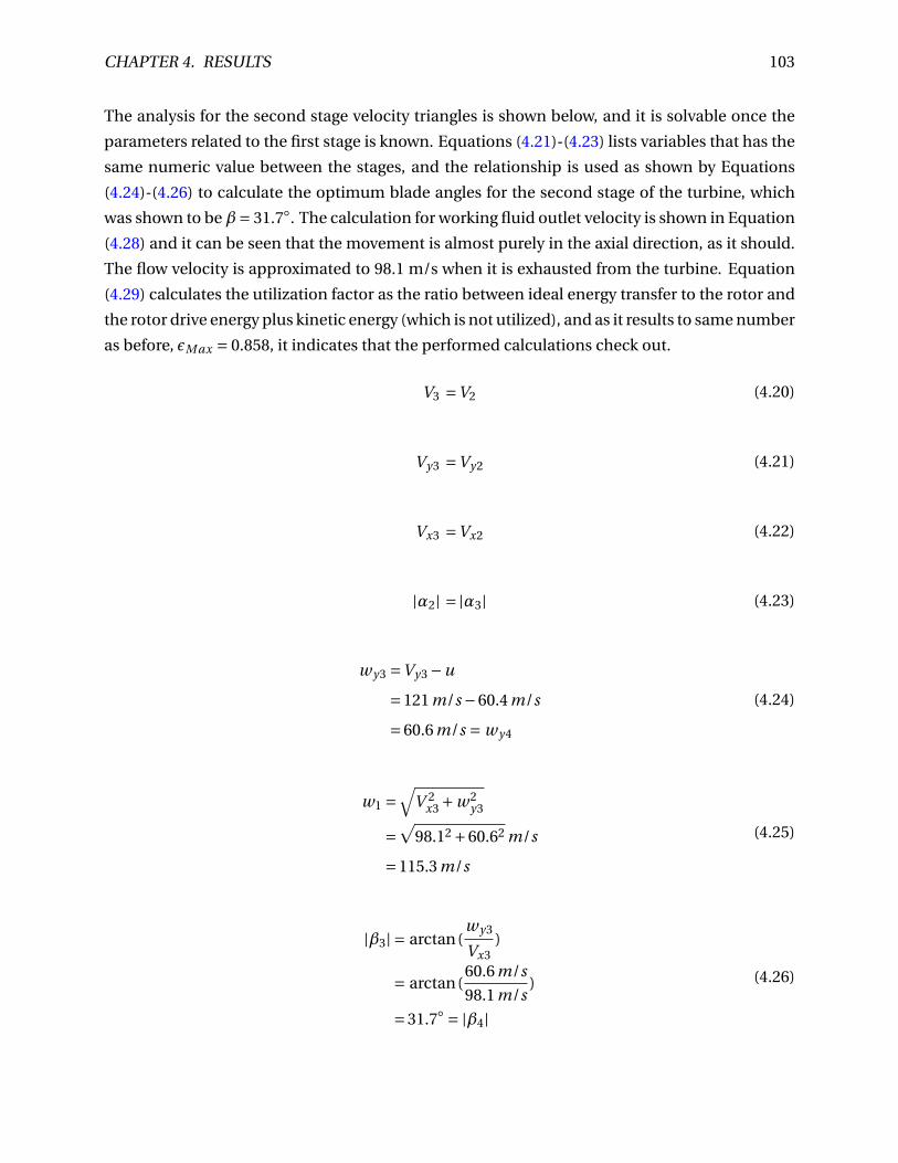
CHAPTER 4. RESULTS 103
The analysis for the second stage velocity triangles is shown below, and it is solvable once the
parameters related to the first stage is known. Equations (4.21)-(4.23) lists variables that has the
same numeric value between the stages, and the relationship is used as shown by Equations
(4.24)-(4.26) to calculate the optimum blade angles for the second stage of the turbine, which
was shown to beβ= 31.7◦. The calculation for working fluid outlet velocity is shown in Equation
(4.28) and it can be seen that the movement is almost purely in the axial direction, as it should.
The flow velocity is approximated to 98.1 m/s when it is exhausted from the turbine. Equation
(4.29) calculates the utilization factor as the ratio between ideal energy transfer to the rotor and
the rotor drive energy plus kinetic energy (which is not utilized), and as it results to same number
as before, εM ax = 0.858, it indicates that the performed calculations check out.
V3 =V2 (4.20)
Vy3 =Vy2 (4.21)
Vx3 =Vx2 (4.22)
|α2| = |α3| (4.23)
wy3 =Vy3 −u
=121 m/s −60.4 m/s
=60.6 m/s = wy4
(4.24)
w1 =√
V 2x3 +w 2
y3
=√
98.12 +60.62 m/s
=115.3 m/s
(4.25)
|β3| = arctan(wy3
Vx3)
= arctan(60.6 m/s
98.1 m/s)
=31.7◦ = |β4|
(4.26)

CHAPTER 4. RESULTS 104
Vy4 =wy4 −u
=60.6 m/s −60.4 m/s
=0.2 m/s ≈ 0
(4.27)
V4 =√
V 2y4 +V 2
x4
=√
0.22 +98.12 m/s
=98.1 m/s
(4.28)
ε= ETot al
ETot al +V 24 /2
= 8u2
8u2 +V 24 /2
= 8×60.42
8×60.42 +98.12/2
=0.858
(4.29)
The turbine selected for the subsea ORC at Tordis needs to be tailored to maximize the utiliza-
tion factor, and if it is opted to use a two-stage turbine with velocity compounding design then
the final design parameters will be of similar values to what has been estimated in this section.
Referring to SIEMENS (2014), an industrial ORC turbine that has standard design traits very sim-
ilar to the subsea cycle requirements is the Siemens SST-060. It is known for its high reliability
under tough working conditions and can produce up to 6 MW gross power. The base design is
pressure rated for up to 131 bara at the inlet side and 29 bara at the outlet, so the custom unit
for the Tordis ORC would have to be rated for slightly higher outlet pressure than the standard
design since it will be operating subsea. A summary of the SST-060 specifications is listed in
Table 4.13, and Figure 4.21 shows how the unit looks.

CHAPTER 4. RESULTS 105
Table 4.13: Siemens SST-060 technical data, dimensions and general features. Information taken fromSIEMENS (2014)
Power Output <6 MWInlet Pressure <131 baraOutlet Pressure <29 baraInlet Temperature <530◦ C
Length 1.5 mWidth 2.5 mHeight 2.5 m
Customizable YesControl valves YesSuitable for ORC YesSuitable for gas expansion Yes
Figure 4.21: Animated illustration of the Siemens SST-060. Figure taken from SIEMENS (2014).

Chapter 5
Conclusions, Discussion, and
Recommendations for Further Work
5.1 Summary and Conclusions
The raw thermal power potential of a well producing from an oil reservoir has been compared
to a well producing from a gas reservoir. Mol fractions from the Tordis field were used as com-
position for the oil and Midgard fluid composition were used for the gas producer. Both cases
were simulated using a production mass rate of 192.5 kg/s with wellhead temperatures ranging
between 50-115◦C. The results were plotted in Figure 4.6 and showed that the Tordis wellstream,
consisting of 31.5 kg/s of oil and 161 kg/s of water, has considerably higher raw thermal potential
than Midgard saturated gas for the entire wellhead temperature range. In fact, as WHT increases
it is increasingly more beneficiary to exploit heat from Tordis compared to Midgard.
In Section 4.1 it were investigated how the raw power potential of the Tordis field varies over
time, using monthly average NPD field data as input for the calculations. The results are shown
in Figure 4.4 and it can be seen that the raw thermal potential was around 14 MW between the
years 1994-1999, when the wells were still producing at zero water cut. After water influx the
potential were essentially doubled from year 2000 to year 2010, then followed the same trend as
the oil production as it decreased towards year 2012. Production increase were seen from year
2013 to 2017 and the calculated values for the raw thermal power potential have increased over
that period as well.
A literature review of general thermodynamic phenomena and on low temperature organic Rank-
ine cycles (LTORC) were performed to support a qualitative thermal feasibility assessment of
using ORC technology subsea at the Tordis field on the Norwegian continental shelf, to convert
geothermal waste heat to usable electricity. Several research articles involving LTORC were re-
106

CHAPTER 5. CONCLUSIONS 107
viewed, but none involving a subsea application specifically. The Tordis field is producing 31.5
kg/s of oil and 161 kg/s of water at approximately 75◦C wellhead temperature. Based on the lit-
erature review, the thermal efficiency of a system working with a heat source bounded by these
constraints is realistically 9-14% at the highest. The most efficient systems have easy access to
an effective coolant and use a cycle working fluid perfectly suited to operate between heat sink
and heat source. Dong et al. (2017) found that use of a suited zeotropic mixture as cycle working
fluid would increase the thermal efficiency compared to using a pure substance, but it would
require a larger heat exchanger area because a bigger portion of the heat transfer happens dur-
ing working fluid phase change. The author of this thesis received a data set containing thermal
properties of the Tordis wellstream from Equinor ASA, and as seen in Section 2.2.1 a PVTsim
flash showed a raw thermal heat potential at 46.5 MW. Under the assumption that 46.5 MW of
heat could be transferred from the wellstream to the cycle working fluid, 9% thermal efficiency
would mean a net power output of 4.19 MW from the generator which would be enough to cover
the fields boosting requirements at around 4 MW. In conclusion the qualitative thermal feasibil-
ity assessment showed that using ORC power generation for boosting can be viable, but would
require no thermal efficiency loss of subsea cycle application as compared to onshore, and that
46.5 MW of heat can be transferred by heat exchanger at these conditions.
A quantitative thermal feasibility assessment were performed to numerically determine the vi-
ability of a subsea ORC plant at Tordis. In order to get information on what heat transfer from
wellstream to cycle that can realistically achieved and to learn the consequence on thermal ef-
ficiency of placing the ORC subsea, a series of thermodynamic models have been used. Aspen
HYSYS were used to represent the Tordis ORC, using a basic cycle configuration consisting of
a pump, an evaporator, a turbine and a condenser. The condenser coolant were modelled as
an isothermal heat sink of water at 9◦C and the evaporator heat source were modeled using the
Tordis composition and rates, at wellhead temperatures ranging between 50-115◦C. In total 37
substances were evaluated as working fluids for the cycle. The fluids R134a and butane per-
formed with high thermal efficiency at onshore ambient pressures, respectively at 11.3% and
10%. When the potential working fluids were tested reacting to a subsea environment at 250m
depth, it were shown that the previously best performing substances could not be evaporated
efficiently at the present temperature and pressure level. The highest thermal efficiency were
achieved using a zeotropic mixture between ethane and propane, with up to 18 mol-% of the
blend being propane. A mixture of 10 mol-% propane and 90 mol-% ethane were chosen as final
composition for the subsea ORC working fluid, because it were opted to go for a slightly lighter
fluid to enable cycle operation at a higher minimum pressure than 250m subsea ambient.

CHAPTER 5. CONCLUSIONS 108
With the selected working fluid, it were possible to make a realistic subsea model of the ORC. To
take advantage of the isothermal heat sink which is the North Sea, a passive cooling manifold
were proposed as replacement for the shell and tube condenser that is generally used in ORCs
onshore. The cooling manifold effective area was estimated to be at least 950 m2 and weigh 36
tonnes when filled with working fluid condensate. The cooling manifold outlet pressure were
modelled as being 30 bars, a few bars higher than natural pressure at 26 bars. The working fluid
is modelled as being at 14.4◦C upon leaving the cooling system, and will be a sub-cooled liquid
at this level of pressure and temperature. The working fluid flows with a mass rate of 81.0 kg/s
through the pump working at 80% isentropic efficiency, which boosts the cycle pressure to 65.0
bars at 21.7◦C.
The heating system is modelled as a series of five dual pass shell and tube heat exchangers with
700 5.25-meter tubes in each. The effective area of the heating train is estimated to 1397.8 m2
before design margin is added to account for fouling. The total heat transferred from wellstream
to cycle with such configuration is 23.2 MW, effectively bringing the temperature of the working
fluid to 70.73◦C at 63.76 bars at evaporator outlet. As the reader may have noticed, this figure
for realistic heat transfer is only approximately half of the ideal heat transfer of 46.5 MW esti-
mated earlier. The working fluid is at a superheated state at these conditions and it is assumed
no energy loss until it flows into the expander inlet. The turbine is modelled as working at 85%
isentropic efficiency and a net total power output from the generator is calculated to 2.1 MW
corresponding to a cycle thermal efficiency of 9%. The chosen working fluid undergoes a rela-
tively high pressure and temperature drop across the expander while still being in gaseous phase
at expander outlet, this being respectively 31 bars and 22◦C. The required basic features of the
turbine were determined when it were assumed a two-stage unit of the axial type, designed us-
ing the velocity compounding technique. It was shown that the working fluid velocity at turbine
inlet should be 260.8 m/s for maximum utilization, which means the pipe leading from evap-
orator to turbine should be sized appropriately to suit this requirement. The rotor blades will
rotate at 60.4 m/s tip speeds and installing blade lengths of 0.19 meters at the turbine inlet side
will tune the production frequency to 50 Hz, in order to correspond with the Norwegian electri-
cal grid frequency. The nozzle angles for both turbine stages were determined to be 67.95◦ and
51◦, and the matching rotor blade angles should be designed as 61.6◦ for stage one and 31.7◦ for
stage two. The axial working fluid velocity leaving the turbine was calculated to 98.1 m/s, which
corresponds to an overall maximum energy utilization efficiency of 85.8%. An industrial tur-
bine that has basic design features rated similar to the subsea ORC requirements is the Siemens
SST-060, which can be customized by Siemens before delivery to adequately cover the needs. In
this case, the custom SST-060 has to be tailored with slightly higher exhaust pressure rating than

CHAPTER 5. CONCLUSIONS 109
the base design. The basic SST-060 is rated for 29 bara exhaust pressures, while the subsea ORC
application would require it to be rated to 31 bara before design margin is added.
Since the model assumes steady state conditions and this is not expected in reality, the following
cycle control elements were chosen as actuators for maximizing electricity production. It is pos-
sible to control the tube side pressure of the heating train using a by-pass valve to circumvent
hydrocarbon vapors and possibly a small fraction of condensate. This helps ensure operation
within the design pressures and will also be used to adjust the liquid fraction entering the heat
exchanger to control the transfer of energy. Since the sea is considered an isothermal heat sink
and abrupt operational changes are not expected, using isolation valves for the sectioned cool-
ing manifold will most likely suffice for regulating the condensation process. These can poten-
tially function as cycle actuators for the condenser outlet temperature if replaced with chokes
for precise day-to-day operational control, or it is possible to use a by-pass cooling system in-
stead for a similar result. It is required to have a high level of accuracy on the cycle pressure
state and working fluid mass rate, of which the main control element is the pump speed. By
controlling the duty supplied to the pump the boosting of the working fluid is actuated, and as
mentioned, pressure drops of the other cycle elements are controlled by the different by-passes.
The final two main control elements required for the subsea ORC are a turbine by-pass valve
and a rotor speed controller. The rotor speed is a direct way of controlling the energy state of the
working fluid at expander outlet and a gear box is also proposed for determining the frequency
of the produced electricity. The turbine by-pass is not meant to be regulated from day to day,
as it is there to be opened in the event of working fluid condensate droplets appearing in the
expander.
The quantitative thermal feasibility assessment showed that it is possible to achieve the same
thermal efficiency subsea as in onshore ORCs. The main challenge is to design an efficient heat-
ing system when the heat source is a low temperature geothermal resource. In the qualitative
analysis it was worked under the assumption that 46.5 MW worth of heat would be transferred
into the subsea power generation unit, which would bring the wellstream down to an evapora-
tor outlet temperature of 20◦C. During the quantitative work it was shown that a heat transfer
of 23.2 MW is a more realistic value for energy transfer between two fluids using an evaporator
at Tordis. With a net power output of 2.1 MW it can not sufficiently cover boosting duties at 4
MW, and the quantitative thermal feasibility is therefore deemed as low. There are possible im-
provements to the energy conversion system which can potentially increase the net output to
desired level. For example through the use of a dual in-line cycle, where the wellstream flows
from evaporator outlet into a secondary ORC that operates with a working fluid with even lower
boiling point.

CHAPTER 5. CONCLUSIONS 110
5.2 Discussion
The raw thermal power potential of the Tordis wellsteam over field lifetime were calculated
based on NPD data of monthly average oil production, GOR, WC and ∆T = 50◦C. The result
showed that a significant increase in thermal power potential took place as water started to flow
with the wellstream, which happened around year 1999. Up until that point, Tordis produced
with a relatively steady oil rate at approximately 12×103 Sm3/d while the gas oil ratio increased
from 91 to 105 Sm3/Sm3 during the same period. The results from the thermal potential calcula-
tion over the duration show a congregated data interval of similar valued data points (with very
few outliers), suggesting that the GOR increase has very little effect on the thermal potential.
A big impact on the potential calculation is seen once water influx takes place into the well-
stream. The water cut increases from 20% at the start of year 2000 to a value of approximately
70% at the beginning of 2008, and during the same time the raw potential is relatively stable
with a slight upwards slope from around 25 MW to 31 MW. One might have expected a higher
thermal power potential increase over the time period since the water cut increased immensely,
but total oil production were decreased from approximately 13×103 Sm3/d to around 3.5×10³
Sm3/d in 2008. This means that while WC were indeed very much increased, the total volumes
of heat energy carrying liquids were not increased by much. In the problem formulation of this
thesis it were mentioned that [...] as increasing water cut leads to more thermal energy potential
over time, a positive synergy effect would be if the heat energy could be used to supply duty to
submerged boosters [...], since boosting requirements increase as fields grow old. These results
point to that while that statement can be true, in reality the thermal potential is not necessar-
ily increasing much between the time of water break through and end of field life. It should be
noted that this assessment were based on past field data and the Tordis production engineers
has worked on minimizing the amount of water produced, as they have had no reason to pro-
duce more significant volumes of liquid water. This means that it is possible to produce more
water with the aim of harvesting geothermal energy, but doing so will most likely not be benefi-
cial due to depletion of the reservoir pressure. Another possibility is to make use of dry confined
wells in the area for geothermal energy production, instead of abandoning them.
In Figure 4.6 the raw power potential of the gas producer Midgard were compared with Tordis
oil and regular water, using the same mass rates, wellhead and outlet temperatures. At 75◦C
the relative difference were around 1.40, with the raw potential of Tordis being 42 MW while
Midgard is at 30 MW. As WHT is increased the benefit from using a liquid based wellstream
is enhanced. At 105◦C the relative difference is 1.44, which points to oil based reservoirs hav-
ing higher thermal potential for any wellhead temperature when the mass rates are equalized.
There are multiple reasons for the increase in energy potential, and it involves phenomena that
were discussed in the general theory chapter of this thesis. When the WHT is increased more of

CHAPTER 5. CONCLUSIONS 111
the water, hydrocarbon and non-condensable gas molecules become into an excited vibrational
and rotational state, making it possible to get a higher meaningful heat transfer upon cooling
the fluid. It should be noted that a gas in general has more entropy (and energy) than a liquid,
but it does not translate into a higher raw potential heat output in our model because it would
be required to condense the gas to harvest the energy as latent heat of condensation.
Selecting an appropriate working fluid in addition to suitable operating parameters for the ORC
is the most important and challenging tasks of all. The choice has a direct impact on the thermal
efficiency, environmental friendliness and final cost of the ORC. Since every application of an
ORC will have a certain amount of available waste heat based on its individual mass flow rates,
heating and cooling temperatures, it is necessary to design the ORC with working fluid and op-
erating parameters for each specific case. In Figure 4.7 the results from a general working fluid
screening based on the Tordis field parameters with ∆T = [TW HT −20◦C] are plotted. The well-
head temperatures that are examined ranges from 50◦C-115◦C, which essentially means that the
heat source can be classified as a low temperature geothermal resource. When WHT is as low
as this it means that certain substances can not function in a subcritical ORC, because it is not
possible to evaporate them with the heating system. The problem is not with the total amount
of raw heat energy since the mass rates are high, the problem is rather that we can not allow
a temperature cross in the evaporator. The plotted results show five fluids that performed well
in the fluid screening, meaning that they could be evaporated with no temperature cross in the
heat exchanger, would be condensed by heat exchange with brine at 9◦C and all this while keep-
ing a vapor fraction of 1 through the expander. R134a is a very commonly used working fluid in
LTORCs in the industry, and also performed with the highest thermal efficiency in this general
screening. When simulated at WH temperatures ranging from 105◦C-115◦C it was seen that the
thermal efficiency of R134a dropped, this because of the expander pressure becoming too high
due to the expansion of the substance, resulting in liquid droplets appearing at the expander
outlet. Therefore, R134a can be credited as the most suited working fluid if WHT is in the range
of 50◦C to 105◦C. i-Butane and n-Butane are easily accessible substances that are contained
in the natural Tordis wellstream, and it can be seen that these hydrocarbons performed really
well at these constraints. No problems occurred when the butanes were subjected to the entire
temperature range, and it can be seen that the butanes net power output curves are becoming
increasingly steep as WHT is increased. The pentanes and hexane also technically fit the ORC
model, but with considerably lower net power output potential.
The ORC thermal efficiency represents the relative fraction of generator energy output to pump
duty and is plotted in Figure 4.8 for the WHT range. At the real Tordis WHT at 75◦C it can be seen
that R134a operates with 11.4% thermal efficiency while i-Butane is at 10.1%, which are values

CHAPTER 5. CONCLUSIONS 112
that seem very good. The calculated thermal efficiencies in the plot should not be analyzed as
absolutes values, but instead only used for direct comparison between the fluids. The reason
is that it were not taken into account isentropic efficiencies of the pump and turbine when the
data was calculated, which means in an application real cycle efficiency would be lower. Figure
4.9 show how the expander inlet pressure reacts to varied WHT for the five potential working flu-
ids. It is easily seen that the pressure increase of R134a is much higher than the others as WHT
is increased, and as mentioned this eventually leads to condensation of liquid droplets from the
gaseous phase. An interesting observation is that the expander inlet pressure ratio over the tem-
perature range is very similar for the different working fluids. At 50◦C WHT it is seen that R134a
is at around 11.9 bars once evaporated and at 105◦C the pressure has increased to almost 40
bars, which equates to a pressure ratio of 3.36 over the WHT range. i-Butane is at 6 bars at 50◦C
WHT and almost 20 when subjected to 105◦C WHT, effectively 3.33 as its pressure ratio across
the temperature range. By looking at the expander inlet pressures at 75◦C WHT it can be seen
that for hexane, pentanes and butanes increasing the evaporator outlet pressure to higher than
10 bars would start forcing the working fluid back into liquid state, since they are saturated with
low degree of superheat. The Tordis wellheads are placed at approximately 250 meters depth,
which means the subsea ambient pressure is around 26 bars. No ORCs in the industry today are
exposed to such a level of natural pressure, and it was found that the recommended working flu-
ids for LTORC are not really suited for a subsea application. Since the cycle minimum pressure
subsea at Tordis should be at least 26 bars, the freedom of choice for subsea ORC is lower than
onshore, making finding a suited working fluid much more of a challenge. In the analysis for
ORC topside it was possible to adjust the pressure minimum using the pump duty to maximize
the thermal efficiency, but as we start looking at subsea specifically the mindset is changed. The
ORC working fluid selection can no longer be solely based on available waste heat, heat source
mass rate and temperature, but it has to be chosen based on how it suits subsea pressures as
well. In the subsea screening model, the pump speed adjusts working fluid mass rate and cycle
pressure minimum to a level above subsea ambient. A suited working fluid that would condense
when subjected to 9◦C coolant at [26 bar+∆Ppump ] while evaporating based on energy from the
Tordis wellstream has to be used in the ORC.
In Figure 4.10 the PT-phase curves of five light fluids present in the Tordis wellstream are plotted,
namely methane, CO2, ethane, propane and i-butane. Some extra tick points have been drawn
onto the plot, these being at 14◦C, 70◦C and 26 bars. An assumption here was that a condenser
heat exchanger would be able to cool the working fluid to within five degrees different from the
temperature of the coolant, so as the sea water is 9◦C the minimum working fluid temperature
of the cycle would potentially be 14◦C. Same assumption were made for the heating system,
the potential highest expected working fluid temperature would be around 70◦C since WHT is
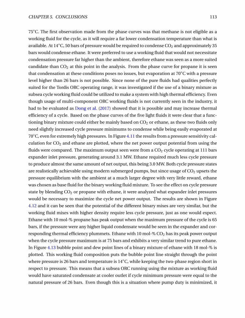
CHAPTER 5. CONCLUSIONS 113
75◦C. The first observation made from the phase curves was that methane is not eligible as a
working fluid for the cycle, as it will require a far lower condensation temperature than what is
available. At 14◦C, 50 bars of pressure would be required to condense CO2 and approximately 35
bars would condense ethane. It were preferred to use a working fluid that would not necessitate
condensation pressure far higher than the ambient, therefore ethane was seen as a more suited
candidate than CO2 at this point in the analysis. From the phase curve for propane it is seen
that condensation at these conditions poses no issues, but evaporation at 70◦C with a pressure
level higher than 26 bars is not possible. Since none of the pure fluids had qualities perfectly
suited for the Tordis ORC operating range, it was investigated if the use of a binary mixture as
subsea cycle working fluid could be utilized to make a system with high thermal efficiency. Even
though usage of multi-component ORC working fluids is not currently seen in the industry, it
had to be evaluated as Dong et al. (2017) showed that it is possible and may increase thermal
efficiency of a cycle. Based on the phase curves of the five light fluids it were clear that a func-
tioning binary mixture could either be mainly based on CO2 or ethane, as these two fluids only
need slightly increased cycle pressure minimums to condense while being easily evaporated at
70◦C, even for extremely high pressures. In Figure 4.11 the results from a pressure sensitivity cal-
culation for CO2 and ethane are plotted, where the net power output potential from using the
fluids were compared. The maximum output seen were from a CO2 cycle operating at 111 bars
expander inlet pressure, generating around 3.1 MW. Ethane required much less cycle pressure
to produce almost the same amount of net output, this being 3.0 MW. Both cycle pressure states
are realistically achievable using modern submerged pumps, but since usage of CO2 upsets the
pressure equilibrium with the ambient at a much larger degree with very little reward, ethane
was chosen as base fluid for the binary working fluid mixture. To see the effect on cycle pressure
state by blending CO2 or propane with ethane, it were analyzed what expander inlet pressures
would be necessary to maximize the cycle net power output. The results are shown in Figure
4.12 and it can be seen that the potential of the different binary mixes are very similar, but the
working fluid mixes with higher density require less cycle pressure, just as one would expect.
Ethane with 10 mol-% propane has peak output when the maximum pressure of the cycle is 65
bars, if the pressure were any higher liquid condensate would be seen in the expander and cor-
responding thermal efficiency plummets. Ethane with 10 mol-% CO2 has its peak power output
when the cycle pressure maximum is at 75 bars and exhibits a very similar trend to pure ethane.
In Figure 4.13 bubble point and dew point lines of a binary mixture of ethane with 18 mol-% is
plotted. This working fluid composition puts the bubble point line straight through the point
where pressure is 26 bars and temperature is 14◦C, while keeping the two-phase region short in
respect to pressure. This means that a subsea ORC running using the mixture as working fluid
would have saturated condensate at cooler outlet if cycle minimum pressure were equal to the
natural pressure of 26 bars. Even though this is a situation where pump duty is minimized, it

CHAPTER 5. CONCLUSIONS 114
is opted to design a cycle that operates on slightly higher pressure minimum than 250 meters
equivalent, so that there will be a safety margin between condensation pressure and the ambi-
ent.
The final operating conditions for the proposed subsea ORC is listed in Table 4.6. The working
fluid selected for modelling were a binary mix of ethane with 10 mol-% propane, which con-
denses at cooling manifold outlet pressure 30 bars and 14.4◦C. The model uses realistic values
for isentropic efficiencies of the rotating equipment and the duty from the heat exchangers are
now based on numerical models. The cycle operates at a thermal efficiency of 9%, with a net
power output of 23260.7 kW from the generator. As 9% thermal efficiency is decent for any ORC,
it is clear that it is not a high pump duty that is bottle necking the energy production. In fact, the
energy transfer from wellstream to working fluid was found to be the limiting factor once a de-
tailed evaporator model was implemented in the simulation. A shell and tube evaporator were
designed in detail in Section 4.7.1 based on the selected working fluid, the Tordis wellstream
and required inlet/outlet conditions. Initial assumptions for the evaporator design were to use
TEMA type BEM made of carbon steel with 25 mm tubes and 31.25 pitch, installed in triangular
tube pattern. Aspen EDR were used to optimize the design with respect to heat transfer, and
it was found that a series of 5 shells with 6 baffles, 2 passes and 700 tubes in each shell would
give the best result. As mentioned earlier, the proposed heating system would give a meaningful
heat transfer of 23.2 MW. This heating duty represents the highest achievable with this setup,
as fouling is likely to occur tube side over time. Net power output potential of the subsea cycle
is estimated to 2.1 MW, which is lower than the target output at 4 MW. To bring the net output
to target level using ORC technology, it would not be enough to change cycle configuration as
it would only slightly increase the thermal efficiency. Instead the engineers would need to in-
crease the amount of energy that flows from wellstream to cycle. When the wellstream flows
out of the evaporator outlet with the current ORC design, it has an estimated temperature of
44.78◦C. This means that it is still at an enthalpy level where the∆T between wellstream and the
sea is significant, meaning it is possible to induce additional heat transfer with a secondary cy-
cle, a so called dual in-line cycle. The secondary cycle would have Tordis field fluids at 44.78◦C
as a energy source and would require a well suited working fluid that can allow operation within
a very small temperature window, approximately between 14-39◦C. The design of a dual in-line
cycle has not been considered in this thesis, but it is plausible that the target output of 4 MW
could be met with such a system. In a feasibility analysis assessing reservoir fluids cooled to
such an extent a big focus should be on flow assurance, as things like hydrates, wax and silica
deposition pose big challenges in a real subsea build.

CHAPTER 5. CONCLUSIONS 115
5.3 Recommendations for Further Work
There is a lot of work remaining before one can determine whether ORC technology has a future
offshore or not. The analysis conducted in this thesis has shown that the amount of available
power is in the mega-watt range, and the potential power output may be acceptable for certain
applications. The author wishes to use this final section to recommend short-, medium- and
long-term extensions to the work presented in this thesis, that is needed to determine if the
thermal energy conversion project would be successful or not.
Short term
A fluid characterization study should be carried out as early as possible. Analyzing the fluid can
provide additional information that would give a more accurate description of the hypotethi-
cal components used in the thermodynamic models. An even more important reason to further
studying the resource (both brine and hydrocarbons) is to get an overview over how big of a tem-
perature drop that can be allowed before precipitation of solids occur. As petroleum engineers,
the focus is usually on staying above the hydrate formation curve or to avoid wax deposition,
but dealing with this technology it must also be ensured that silica, stibnite or similar solids do
not deposit from the chilling brine. If the results from the fluid analysis show that the wellstream
can be cooled the required amount without issues, it is proposed to approach dealers in the in-
dustry to get early cost estimates for the various components of the cycle. The Tordis wellstream
offer two things "for free", the energy potential and the chosen working fluid (can be separated
from the gaseous phase), all other equipment must be bought custom designed for the operat-
ing conditions. The information gathered at this point should suffice to determine costs related
to operation and annual maintenance, and finally estimate the payback period for the project.
Medium term
The medium-term objective recommendation is rather simple. After cooling capabilities of the
working fluid and rate of return have been estimated with acceptable degree of accuracy, one
can revisit the cycle configuration. If the wellstream fluid can be cooled to a larger extent than
the proposed ORC system is designed for, and the costs are reasonable, it is possible that a dual
in-line ORC can be considered. The dual in-line cycle operates in the same fashion as basic ORC,
but is really a series of two basic cycles. The added cycle uses a working fluid with lower boiling
point than the current and will make it viable to cool the Tordis wellstream to a lower value than
44.7◦C. The result would essentially be larger heat transfer from wellstream to the cycles, and
the net power output would increase.
CHAPTER 5. CONCLUSIONS 116
Long term
The final stage is to design everything in detail. The cost estimates from the short-term work
were approximates which helped decide final cycle configuration and get an idea of the pay back
period. Requesting tender offers from industrial providers for specific turbines, heat exchangers
and pumps will be part of determining the final costs. If willing to proceed with the project, a
risk assessment based on the proposed equipment design has to be performed. For example,
it has to be quantified how much working fluid is expected to leak from the turbine shaft and
which environmental impact the leak poses. The risk assessment also quantifies financial risks.
An example of a financial risk scenario could be to determine the impact of having a delay in
the delivery of a vital cycle component. If the ORC were expected to supply energy for boosting
a field, and installation is delayed, the impact could be massive. Once a detailed plan and risk
assessment for commercializing subsea ORC at Tordis is finalised, the true feasibility can be
accurately judged.

Appendix A
Code associated with the Raw Power Model
A.1 Introduction
The following Excel VBA programs was written to link Excel with Aspen HYSYS in order to cal-
culate raw thermal power potential from a fluid stream, to see effects of GOR and WHT changes
along with potential development over a fields lifetime.
A.1.1 Tordis power potential over its lifetime VBA
This script was only included for reference, and will be impossible to run without the corre-
sponding Excel document and HYSYS file. Therefore no "cleaning" of the code was performed
before attachment.
Listing A.1: Visual basic code used for Tordis field lifetime calculation.
1 Option Explicit2 Public hyApp As HYSYS.Application3 Public simCase As SimulationCase4 Public pStream As ProcessStream5 Public Stream_1 As ProcessStream6 Public Stream_2 As ProcessStream7 Public giStream As ProcessStream8 Public oiStream As ProcessStream9 Public g0Stream As ProcessStream
10 Public o0Stream As ProcessStream11 Public mixedStream As ProcessStream12 Public InletStream As ProcessStream13 Public waterStream As ProcessStream14 Public feed1Stream As ProcessStream
117

APPENDIX A. CODE ASSOCIATED WITH THE RAW POWER MODEL 118
15 Public out1Stream As ProcessStream16 Public q1Stream As ProcessStream17
18
19 Public filename As String20 Public ITEM As Integer21 Public SS As Object22 Dim hyPhase As FluidPhase23 Dim hyPhases As FluidPhases24 Dim hyFluid As Fluid25 Dim feed1hyFluid As Fluid26 Dim out1hyFluid As Fluid27 Dim hyPhaseOut As FluidPhase28 Dim hyPhasesOut As FluidPhases29 Dim hyFluidOut As Fluid30 Dim i As Integer31 Dim itr As Integer32 Public Sub StartHYSYS_SurfaceProcessing ()33 Dim filename As String34 Dim ITEM As Integer35 Dim Compositions As Variant36 Dim gasCompositions As Variant37 Dim oilCompositions As Variant38 Dim feedCompositions As Variant39 Dim GOR As Integer40 Dim rad As Integer41 Dim qo As Variant42 Dim qo_temp As Variant43 Dim factor As Variant44
45 ’Load HYSYS file46 Set hyApp = CreateObject("HYSYS.Application")47 hyApp.Visible = True48 Set simCase = hyApp.ActiveDocument49 If simCase Is Nothing Then50 filename = Worksheets("HYSYS_PowerVsTime_Norne").
Range("C4").Text51 If filename <> "False" And simCase Is Nothing Then

APPENDIX A. CODE ASSOCIATED WITH THE RAW POWER MODEL 119
52 Set simCase = GetObject(filename , "HYSYS.SimulationCase")
53 simCase.Visible = True54 End If55 End If56
57 ’Code to read data from Excel into HYSYS components58 Set pStream = simCase.Flowsheet.MaterialStreams.ITEM("
InitialComp")59 Set InletStream = simCase.Flowsheet.MaterialStreams.ITEM("Inlet
stream")60 Set Stream_1 = simCase.Flowsheet.MaterialStreams.ITEM("1")61 Set Stream_2 = simCase.Flowsheet.MaterialStreams.ITEM("2")62 Set giStream = simCase.Flowsheet.MaterialStreams.ITEM("g-i")63 Set oiStream = simCase.Flowsheet.MaterialStreams.ITEM("o-i")64 Set g0Stream = simCase.Flowsheet.MaterialStreams.ITEM("g-0")65 Set o0Stream = simCase.Flowsheet.MaterialStreams.ITEM("o-0")66 Set feed1Stream = simCase.Flowsheet.MaterialStreams.ITEM("FEED
-1")67 Set out1Stream = simCase.Flowsheet.MaterialStreams.ITEM("OUT -1"
)68 Set q1Stream = simCase.Flowsheet.EnergyStreams.ITEM("Q-1")69 Set waterStream = simCase.Flowsheet.MaterialStreams.ITEM("Water
")70
71 ’Feed fluid72 Set hyFluid = pStream.DuplicateFluid73 Set hyPhases = hyFluid.FluidPhases74
75 ’For Z factor retrieval76 Set feed1hyFluid = feed1Stream.DuplicateFluid77 Set out1hyFluid = out1Stream.DuplicateFluid78
79 ’Compositions = pStream.ComponentMolarFractionValue80 ’gasCompositions = g0Stream.ComponentMolarFractionValue81 ’oilCompositions = o0Stream.ComponentMolarFractionValue82 ’For ITEM = 0 To 11 ’collecting composition data as
variant

APPENDIX A. CODE ASSOCIATED WITH THE RAW POWER MODEL 120
83 ’ Compositions(ITEM) = Worksheets ("HYSYS_SurfaceProcessing ").Range("D" & ITEM + 7).Value
84 ’Next ITEM85
86
87 ’For ITEM = 0 To 11 ’collecting composition data asvariant
88 ’ Cells(ITEM + 7, 8) = giStream.ComponentMolarFractionValue(ITEM)
89 ’ Cells(ITEM + 7, 12) = oiStream.ComponentMolarFractionValue(ITEM)
90 ’ gasCompositions(ITEM) = Worksheets ("HYSYS_SurfaceProcessing ").Range ("H" & ITEM + 7).Value
91 ’ oilCompositions(ITEM) = Worksheets ("HYSYS_SurfaceProcessing ").Range ("L" & ITEM + 7).Value
92 ’Next ITEM93
94 ’ apply composition data95 ’pStream.ComponentMolarFraction.Values = Compositions96 ’g0Stream.ComponentMolarFraction.Values = gasCompositions97 ’o0Stream.ComponentMolarFraction.Values = oilCompositions98
99 ’g0Stream.MolarFlow.SetValue Cells (21, 8), "m3/d_(gas)"100 ’o0Stream.MolarFlow.SetValue Cells (21, 12), "m3/d_(gas)"101 ’g0Stream.MolarFlow.SetValue Cells (21, 8), "kgmole/h"102 ’o0Stream.MolarFlow.SetValue Cells (21, 12), "kgmole/h"103
104
105 ’WH Temperature and Pressure and flow rate from Excel106 pStream.TemperatureValue = Cells(23, 4)107 pStream.Pressure.SetValue Cells (24, 4), "bar"108
109 ’InletStream.TemperatureValue = Cells (23, 4)110 InletStream.Pressure.SetValue Cells (24, 4), "bar"111
112 g0Stream.TemperatureValue = Cells(23, 4)113 g0Stream.Pressure.SetValue Cells(24, 4), "bar"114 o0Stream.TemperatureValue = Cells(23, 4)

APPENDIX A. CODE ASSOCIATED WITH THE RAW POWER MODEL 121
115 o0Stream.Pressure.SetValue Cells(24, 4), "bar"116
117 Stream_1.TemperatureValue = Cells(25, 4)118 Stream_1.Pressure.SetValue Cells(26, 4), "bar"119 Stream_2.TemperatureValue = Cells(27, 4)120 Stream_2.Pressure.SetValue Cells(28, 4), "bar"121
122 feed1Stream.TemperatureValue = Cells(23, 4)123 feed1Stream.Pressure.SetValue Cells (24, 4), "bar"124 out1Stream.TemperatureValue = feed1Stream.TemperatureValue -
Cells(4, 16) ’Out Temp = In Temp minus dT125 out1Stream.Pressure.SetValue Cells (32, 4), "bar"126
127
128 feedCompositions = feed1Stream.ComponentMolarFractionValue129 Set SS = simCase.Flowsheet.Operations.ITEM("SS_GOR")130 ’Initial value for produced molerate of oil131 o0Stream.MolarFlow.SetValue 400, "kgmole/h"132 g0Stream.MolarFlow.SetValue 200, "kgmole/h"133 For rad = 40 To 296134 SS.Cell("C2").CellValue = Cells(rad , 3) ’Defining GOR in SS_GOR
in HYSYS135
136 ’Find qo137 SS.Cell("C5").CellValue = Cells(rad , 5)138 ’Find wc139 SS.Cell("D2").CellValue = Cells(rad , 4)140
141
142 While SS.Cell("A2").CellValue * 3600 < SS.Cell("C5").CellValue143 SS.Cell("A4").CellValue = o0Stream.MolarFlow.GetValue("kgmole
/h")144 o0Stream.MolarFlow.SetValue (SS.Cell("A4").CellValue + 10), "
kgmole/h"145 Application.Wait Now + 1 / (24 * 60 * 60# * 2)146 Wend147
148

APPENDIX A. CODE ASSOCIATED WITH THE RAW POWER MODEL 122
149 ’Store value for molerate of oil in spreadsheet150 For ITEM = 0 To 22 ’collecting composition data as
variant151 feedCompositions(ITEM) = InletStream.
ComponentMolarFractionValue(ITEM)152 Next ITEM153 Application.Wait Now + 1 / (24 * 60 * 60# * 2)154 waterStream.StdLiqVolFlow.Value = SS.Cell("D7").CellValue155 feed1Stream.ComponentMolarFraction.Values = feedCompositions156 feed1Stream.MolarFlow.Value = InletStream.MolarFlow.Value ’
Flow rate from "Inlet stream" to "FEED -1"157 Cells(rad , 6) = feed1Stream.MassFlow.GetValue("kg/h")158 Cells(rad , 7) = q1Stream.HeatFlow.GetValue("kJ/h")159 ’Enthalpy160 Cells(rad , 8) = feed1Stream.MassEnthalpyValue161 Cells(rad , 9) = out1Stream.MassEnthalpyValue162 ’Deviation factor (Z factor)163 Cells(rad , 10) = feed1hyFluid.VapourPhase.CompressibilityValue164 Cells(rad , 11) = out1hyFluid.VapourPhase.CompressibilityValue165
166 ’Reset to low production values to make sure while sentencewill work
167 While SS.Cell("A2").CellValue * 3600 > Cells(rad + 1, 5)168 ’While o0Stream.MolarFlow.GetValue (" kgmole/h") > 4500169 o0Stream.MolarFlow.SetValue (o0Stream.MolarFlow.GetValue("
kgmole/h") - 30), "kgmole/h"170 Application.Wait Now + 1 / (24 * 60 * 60# * 2)171 Wend172
173
174
175 Next rad176
177
178 ThisWorkbook.Save179
180 End Sub

APPENDIX A. CODE ASSOCIATED WITH THE RAW POWER MODEL 123
A.1.2 Code for quick heat transfer calculation based on ∆T and fluid com-
position
This script was only included for reference, and will be impossible to run without the corre-
sponding Excel document and HYSYS file. Therefore no "cleaning" of the code was performed
before attachment.
Listing A.2: Visual basic code for estimating raw power potential when WHT is fixed.
1 Option Explicit2 Public hysApp As HYSYS.Application3 Public simCase As SimulationCase4 Public filename As String5 Public Sub HYSYS_Raw_Potential ()6 Dim WATERinStream As ProcessStream7 Dim HCinStream As ProcessStream8 Dim WELLSTREAMinStream As ProcessStream9 Dim WELLSTREAMoutStream As ProcessStream
10 Dim RawPotentialStream As ProcessStream11
12 ’Code to load HYSYS simulation file13 Set hysApp = CreateObject("HYSYS.Application")14 hysApp.Visible = True15 Set simCase = hysApp.ActiveDocument16 If simCase Is Nothing Then17 filename = Worksheets("Raw_Potential_Tordis").Range("
B2").Text18 If filename <> "False" And simCase Is Nothing Then19 Set simCase = GetObject(filename , "HYSYS.
SimulationCase")20 simCase.Visible = True21 End If22 End If23
24 ’Code to specify input data from Excel into HYSYS components25 ’Material streams26 Set WATERinStream = simCase.Flowsheet.MaterialStreams.Item("HT -
Water")27 Set HCinStream = simCase.Flowsheet.MaterialStreams.Item("HT-HC"
)
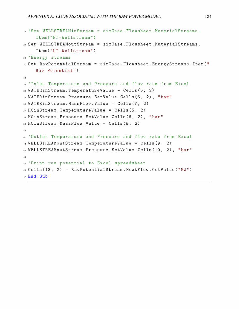
APPENDIX A. CODE ASSOCIATED WITH THE RAW POWER MODEL 124
28 ’Set WELLSTREAMinStream = simCase.Flowsheet.MaterialStreams.Item("HT-Wellstream ")
29 Set WELLSTREAMoutStream = simCase.Flowsheet.MaterialStreams.Item("LT-Wellstream")
30 ’Energy streams31 Set RawPotentialStream = simCase.Flowsheet.EnergyStreams.Item("
Raw Potential")32
33 ’Inlet Temperature and Pressure and flow rate from Excel34 WATERinStream.TemperatureValue = Cells(5, 2)35 WATERinStream.Pressure.SetValue Cells(6, 2), "bar"36 WATERinStream.MassFlow.Value = Cells(7, 2)37 HCinStream.TemperatureValue = Cells(5, 2)38 HCinStream.Pressure.SetValue Cells(6, 2), "bar"39 HCinStream.MassFlow.Value = Cells(8, 2)40
41 ’Outlet Temperature and Pressure and flow rate from Excel42 WELLSTREAMoutStream.TemperatureValue = Cells(9, 2)43 WELLSTREAMoutStream.Pressure.SetValue Cells(10, 2), "bar"44
45 ’Print raw potential to Excel spreadsheet46 Cells(13, 2) = RawPotentialStream.HeatFlow.GetValue("MW")47 End Sub

APPENDIX A. CODE ASSOCIATED WITH THE RAW POWER MODEL 125
A.1.3 Code for quick heat transfer calculation based on ∆T and fluid com-
position over entire WHT range
This script was only included for reference, and will be impossible to run without the corre-
sponding Excel document and HYSYS file. Therefore no "cleaning" of the code was performed
before attachment.
Listing A.3: Visual basic code for estimating raw power potential when WHT is varied.
1 Public Sub HYSYS_Raw_Potential_Sensitivity ()2 Dim WATERinStream As ProcessStream3 Dim HCinStream As ProcessStream4 Dim WELLSTREAMinStream As ProcessStream5 Dim WELLSTREAMoutStream As ProcessStream6 Dim RawPotentialStream As ProcessStream7 Dim i As Integer8
9 ’Code to load HYSYS simulation file10 Set hysApp = CreateObject("HYSYS.Application")11 hysApp.Visible = True12 Set simCase = hysApp.ActiveDocument13 If simCase Is Nothing Then14 filename = Worksheets("Raw_Potential_Tordis").Range("
B2").Text15 If filename <> "False" And simCase Is Nothing Then16 Set simCase = GetObject(filename , "HYSYS.
SimulationCase")17 simCase.Visible = True18 End If19 End If20
21 ’Code to specify input data from Excel into HYSYS components22 ’Material streams23 Set WATERinStream = simCase.Flowsheet.MaterialStreams.Item("HT -
Water")24 Set HCinStream = simCase.Flowsheet.MaterialStreams.Item("HT-HC"
)25 ’Set WELLSTREAMinStream = simCase.Flowsheet.MaterialStreams.
Item("HT-Wellstream ")26 Set WELLSTREAMoutStream = simCase.Flowsheet.MaterialStreams.

APPENDIX A. CODE ASSOCIATED WITH THE RAW POWER MODEL 126
Item("LT-Wellstream")27 ’Energy streams28 Set RawPotentialStream = simCase.Flowsheet.EnergyStreams.Item("
Raw Potential")29
30 ’Inlet Pressure and flow rate from Excel31 WATERinStream.Pressure.SetValue Cells(6, 2), "bar"32 WATERinStream.MassFlow.Value = Cells(7, 2)33 HCinStream.TemperatureValue = Cells(5, 2)34 HCinStream.Pressure.SetValue Cells(6, 2), "bar"35 HCinStream.MassFlow.Value = Cells(8, 2)36
37 ’Outlet Temperature and Pressure and flow rate from Excel38 WELLSTREAMoutStream.TemperatureValue = Cells(9, 2)39 WELLSTREAMoutStream.Pressure.SetValue Cells(10, 2), "bar"40
41 For i = 0 To (Cells(20, 3) - Cells(20, 2))42 Cells (23 + i, 1) = Cells(20, 2) + i ’Printing temperature range
from A2343 Cells (23 + i, 2) = i + 1 ’Printing iteration number from B2344 ’Inlet Temperature and Pressure and flow rate from Excel45 WATERinStream.TemperatureValue = Cells (23 + i, 1)46 HCinStream.TemperatureValue = Cells (23 + i, 1)47 ’Print raw potential to Excel spreadsheet48 Cells (23 + i, 3) = RawPotentialStream.HeatFlow.GetValue("MW")49 Next i50
51 End Sub

Appendix B
Code associated with the Subsea ORC Model
B.1 Introduction
The following Excel VBA programs was written to link Excel with Aspen HYSYS in order to cal-
culate ORC basic cycle properties based on specifications defined in the spreadsheet and print
the results. The code calls based on a lot of cell coordinates which correspond to those shown
in Figure B.1.
Cell coordinates referenced in code
Figure B.1: The scripts in Appendix B references the variables in this figure.
127

APPENDIX B. CODE ASSOCIATED WITH THE SUBSEA ORC MODEL 128
B.1.1 Code for calculation of basic ORC properties
This script was only included for reference, and will be impossible to run without the corre-
sponding Excel document and HYSYS file. Therefore no "cleaning" of the code was performed
before attachment.
Listing B.1: Visual basic code for estimation and print basic ORC properties
1 Public Sub HYSYS_Basic_Cycle ()2 Dim SS As Object3 Dim Compositions As Variant4 Dim WF As Integer5 Dim condensateStream As ProcessStream6
7 ’Code to load HYSYS simulation file8 Set hysApp = CreateObject("HYSYS.Application")9 hysApp.Visible = True
10 Set simCase = hysApp.ActiveDocument11 If simCase Is Nothing Then12 filename = Worksheets("Raw_Potential_Tordis").Range("
B2").Text13 If filename <> "False" And simCase Is Nothing Then14 Set simCase = GetObject(filename , "HYSYS.
SimulationCase")15 simCase.Visible = True16 End If17 End If18
19 Set condensateStream = simCase.Flowsheet.MaterialStreams.Item("Condensate (3)")
20 Compositions = condensateStream.ComponentMolarFractionValue21 For WF = 0 To 43 ’collecting composition data as variant22 Compositions(WF) = Worksheets("Raw_Potential_Tordis")
.Range("I" & WF + 23).Value23 Next WF24 ’ apply composition data25 condensateStream.ComponentMolarFraction.Values = Compositions26
27 Set SS = simCase.Flowsheet.Operations.Item("Cycle Summary")28 SS.Cell("B2").CellValue = Cells(6, 12)

APPENDIX B. CODE ASSOCIATED WITH THE SUBSEA ORC MODEL 129
29 SS.Cell("B4").CellValue = Cells(8, 12)30 SS.Cell("B8").CellValue = Cells(12, 12)31 ’SS.Cell("C4").CellValue = Cells(8, 13) * 10032 Cells(8, 13) = SS.Cell("C4").CellValue * 0.0133 SS.Cell("D2").CellValue = Cells(6, 14)34 SS.Cell("D4").CellValue = Cells(8, 14)35 SS.Cell("E8").CellValue = Cells(16, 14)36 SS.Cell("E9").CellValue = Cells(17, 14)37 Cells(7, 12) = SS.Cell("B3").CellValue38 Cells(9, 12) = SS.Cell("B5").CellValue39 Cells(13, 12) = SS.Cell("B9").CellValue40 Cells(6, 13) = SS.Cell("C2").CellValue * 0.0141 Cells(7, 13) = SS.Cell("C3").CellValue * 0.0142 Cells(9, 13) = SS.Cell("C5").CellValue * 0.0143 Cells(7, 14) = SS.Cell("D3").CellValue44 Cells(9, 14) = SS.Cell("D5").CellValue45 Cells(16, 12) = SS.Cell("D8").CellValue46 Cells(17, 12) = SS.Cell("D9").CellValue47 Cells(18, 12) = SS.Cell("D10").CellValue48 Cells(19, 12) = SS.Cell("D11").CellValue49 End Sub
B.1.2 Code for calculation of basic ORC properties when WHT is varied.
This script was only included for reference, and will be impossible to run without the corre-
sponding Excel document and HYSYS file. Therefore no "cleaning" of the code was performed
before attachment.
Listing B.2: Visual basic code for estimation and print basic ORC properties for a series of WHT values.
1 Public Sub HYSYS_Basic_Cycle_Sensitivity ()2 Dim SS As Object3 Dim j As Integer4 Dim Compositions As Variant5 Dim WF As Integer6 Dim condensateStream As ProcessStream7
8 ’Code to load HYSYS simulation file9 Set hysApp = CreateObject("HYSYS.Application")

APPENDIX B. CODE ASSOCIATED WITH THE SUBSEA ORC MODEL 130
10 hysApp.Visible = True11 Set simCase = hysApp.ActiveDocument12 If simCase Is Nothing Then13 filename = Worksheets("Raw_Potential_Tordis").Range("
B2").Text14 If filename <> "False" And simCase Is Nothing Then15 Set simCase = GetObject(filename , "HYSYS.
SimulationCase")16 simCase.Visible = True17 End If18 End If19
20 Set condensateStream = simCase.Flowsheet.MaterialStreams.Item("Condensate (3)")
21 Compositions = condensateStream.ComponentMolarFractionValue22 For WF = 0 To 43 ’collecting composition data as variant23 Compositions(WF) = Worksheets("Raw_Potential_Tordis")
.Range("I" & WF + 23).Value24 Next WF25 condensateStream.ComponentMolarFraction.Values = Compositions26
27 Set SS = simCase.Flowsheet.Operations.Item("Cycle Summary")28 SS.Cell("B2").CellValue = Cells(6, 12)29 SS.Cell("B4").CellValue = Cells(8, 12)30 SS.Cell("B8").CellValue = Cells (12, 12)31 ’SS.Cell("C4").CellValue = Cells(8, 13) * 10032
33 SS.Cell("D2").CellValue = Cells(6, 14)34 SS.Cell("D4").CellValue = Cells(8, 14)35 SS.Cell("E8").CellValue = Cells (16, 14)36 SS.Cell("E9").CellValue = Cells (17, 14)37
38 ’to reset39 SS.Cell("B4").CellValue = Cells(8, 12)40 Cells (23 + 0, 11) = Cells (20, 2) + 0 ’Printing temperature
range from A2341 Cells (23 + 0, 12) = 0 + 1 ’Printing iteration number from B2342 Cells (23 + 0, 13) = Cells (23 + 0, 3) * 1000 ’Boiler duty

APPENDIX B. CODE ASSOCIATED WITH THE SUBSEA ORC MODEL 131
43 Cells(12, 12) = Cells (23 + 0, 3) * 100044 Cells(8, 12) = Cells (23 + 0, 1) - Cells(21, 12) ’Pinch45 Application.Wait Now + #12:00:01 AM#46 Cells (23 + 0, 14) = SS.Cell("D10").CellValue47 Cells (23 + 0, 15) = SS.Cell("D11").CellValue48 Cells (23 + 0, 16) = SS.Cell("C4").CellValue * 0.01 ’Turbine
inlet pressure49 ’end reset50
51 For j = 0 To (Cells(20, 3) - Cells(20, 2))52 Cells (23 + j, 11) = Cells (20, 2) + j ’Printing temperature
range from A2353 Cells (23 + j, 12) = j + 1 ’Printing iteration number from B2354 Cells (23 + j, 13) = Cells (23 + j, 3) * 1000 ’Boiler duty55 Cells(12, 12) = Cells (23 + j, 3) * 100056 Cells(8, 12) = Cells (23 + j, 1) - Cells(21, 12) ’Pinch57 Application.Wait Now + #12:00:01 AM#58 Cells (23 + j, 14) = SS.Cell("D10").CellValue59 Cells (23 + j, 15) = SS.Cell("D11").CellValue60 Cells (23 + j, 16) = SS.Cell("C4").CellValue * 0.01 ’Turbine
inlet pressure61 Cells (23 + j, 17) = SS.Cell("D5").CellValue ’Turbine Exhaust
Vapor Fraction62 SS.Cell("B4").CellValue = Cells(8, 12)63 SS.Cell("B8").CellValue = Cells (12, 12)64 Next j65
66 Cells(8, 13) = SS.Cell("C4").CellValue * 0.0167 Cells(7, 12) = SS.Cell("B3").CellValue68 Cells(9, 12) = SS.Cell("B5").CellValue69 Cells(13, 12) = SS.Cell("B9").CellValue70 Cells(6, 13) = SS.Cell("C2").CellValue * 0.0171 Cells(7, 13) = SS.Cell("C3").CellValue * 0.0172 Cells(9, 13) = SS.Cell("C5").CellValue * 0.0173 Cells(7, 14) = SS.Cell("D3").CellValue74 Cells(9, 14) = SS.Cell("D5").CellValue75 Cells(16, 12) = SS.Cell("D8").CellValue76 Cells(17, 12) = SS.Cell("D9").CellValue

APPENDIX B. CODE ASSOCIATED WITH THE SUBSEA ORC MODEL 132
77 Cells(18, 12) = SS.Cell("D10").CellValue78 Cells(19, 12) = SS.Cell("D11").CellValue79
80 End Sub
B.1.3 Code used for calculation of basic subsea model ORC properties.
This script was only included for reference, and will be impossible to run without the corre-
sponding Excel document and HYSYS file. Therefore no "cleaning" of the code was performed
before attachment.
Listing B.3: Visual basic code for estimation and print properties subsea ORC model.
1 Public Sub HYSYS_Subsea_Cycle_Sensitivity ()2 Dim SS As Object3 Dim j As Integer4 Dim Compositions As Variant5 Dim WF As Integer6 Dim condensateStream As ProcessStream7
8 ’Code to load HYSYS simulation file9 Set hysApp = CreateObject("HYSYS.Application")
10 hysApp.Visible = True11 Set simCase = hysApp.ActiveDocument12 If simCase Is Nothing Then13 filename = Worksheets("Raw_Potential_Tordis").Range("
B2").Text14 If filename <> "False" And simCase Is Nothing Then15 Set simCase = GetObject(filename , "HYSYS.
SimulationCase")16 simCase.Visible = True17 End If18 End If19
20 ’Set condensateStream = simCase.Flowsheet.MaterialStreams.Item(" Condensate (3)")
21 ’Compositions = condensateStream.ComponentMolarFractionValue22 ’For WF = 0 To 41 ’collecting composition data as variant23 ’ Compositions(WF) = Worksheets (" Raw_Potential_Tordis

APPENDIX B. CODE ASSOCIATED WITH THE SUBSEA ORC MODEL 133
").Range ("I" & WF + 23).Value24 ’Next WF25 ’condensateStream.ComponentMolarFraction.Values = Compositions26
27 Set SS = simCase.Flowsheet.Operations.Item("Cycle Summary")28 SS.Cell("B2").CellValue = Cells (102, 2)29 ’SS.Cell("B4").CellValue = Cells (104, 2)30 SS.Cell("B8").CellValue = Cells (108, 2)31 ’SS.Cell("C4").CellValue = Cells(8, 13) * 10032
33 SS.Cell("D2").CellValue = Cells (102, 4)34 SS.Cell("D4").CellValue = Cells (104, 4)35 SS.Cell("E8").CellValue = Cells (108, 5)36 SS.Cell("E9").CellValue = Cells (109, 5)37
38 ’to reset39 SS.Cell("B4").CellValue = Cells (114, 1)40 ’Cells (114 + 0, 11) = Cells (20, 2) + 0 ’Printing temperature
range from A2341 ’Cells (114 + 0, 12) = 0 + 1 ’Printing iteration number from B2342 ’Cells (114 + 0, 13) = Cells (23 + 0, 3) * 1000 ’Boiler duty43 ’Cells (114, 12) = Cells (23 + 0, 3) * 100044 ’Cells(8, 12) = Cells (23 + 0, 1) - Cells(21, 12) ’Pinch45 Application.Wait Now + #12:00:01 AM#46 Cells (114 + 0, 2) = SS.Cell("D10").CellValue47 Cells (114 + 0, 3) = SS.Cell("B3").CellValue48 Cells (114 + 0, 4) = SS.Cell("B4").CellValue49 Cells (114 + 0, 5) = SS.Cell("C2").CellValue * 0.0150 Cells (114 + 0, 6) = SS.Cell("C3").CellValue * 0.0151 Cells (114 + 0, 7) = SS.Cell("C4").CellValue * 0.0152 Cells (114 + 0, 8) = SS.Cell("C5").CellValue * 0.0153 Cells (114 + 0, 9) = SS.Cell("D2").CellValue54 Cells (114 + 0, 10) = SS.Cell("D3").CellValue55 Cells (114 + 0, 11) = SS.Cell("D4").CellValue56 Cells (114 + 0, 12) = SS.Cell("D5").CellValue57 Cells (114 + 0, 13) = SS.Cell("E2").CellValue58 Cells (114 + 0, 14) = SS.Cell("B8").CellValue59 Cells (114 + 0, 15) = SS.Cell("B9").CellValue

APPENDIX B. CODE ASSOCIATED WITH THE SUBSEA ORC MODEL 134
60 Cells (114 + 0, 16) = SS.Cell("D8").CellValue61 Cells (114 + 0, 17) = SS.Cell("D9").CellValue62 Cells (114 + 0, 18) = SS.Cell("D11").CellValue63 ’Cells (114 + 0, 16) = SS.Cell("C4").CellValue * 0.01 ’Turbine
inlet pressure64 ’end reset65
66 For j = 0 To 76 ’ (Cells(20, 3) - Cells (20, 2))67 SS.Cell("B4").CellValue = Cells (114 + j, 1)68 ’Cells (114 + 0, 11) = Cells (20, 2) + 0 ’Printing temperature
range from A2369 ’Cells (114 + 0, 12) = 0 + 1 ’Printing iteration number from B2370 ’Cells (114 + 0, 13) = Cells (23 + 0, 3) * 1000 ’Boiler duty71 ’Cells (114, 12) = Cells (23 + 0, 3) * 100072 ’Cells(8, 12) = Cells (23 + 0, 1) - Cells(21, 12) ’Pinch73 Application.Wait Now + #12:00:01 AM#74 Cells (114 + j, 2) = SS.Cell("D10").CellValue75 Cells (114 + j, 3) = SS.Cell("B3").CellValue76 Cells (114 + j, 4) = SS.Cell("B4").CellValue77 Cells (114 + j, 5) = SS.Cell("C2").CellValue * 0.0178 Cells (114 + j, 6) = SS.Cell("C3").CellValue * 0.0179 Cells (114 + j, 7) = SS.Cell("C4").CellValue * 0.0180 Cells (114 + j, 8) = SS.Cell("C5").CellValue * 0.0181 Cells (114 + j, 9) = SS.Cell("D2").CellValue82 Cells (114 + j, 10) = SS.Cell("D3").CellValue83 Cells (114 + j, 11) = SS.Cell("D4").CellValue84 Cells (114 + j, 12) = SS.Cell("D5").CellValue85 Cells (114 + j, 13) = SS.Cell("E2").CellValue86 Cells (114 + j, 14) = SS.Cell("B8").CellValue87 Cells (114 + j, 15) = SS.Cell("B9").CellValue88 Cells (114 + j, 16) = SS.Cell("D8").CellValue89 Cells (114 + j, 17) = SS.Cell("D9").CellValue90 Cells (114 + j, 18) = SS.Cell("D11").CellValue91 Next j92
93 ’Cells(8, 13) = SS.Cell("C4").CellValue * 0.0194 ’Cells(7, 12) = SS.Cell("B3").CellValue95 ’Cells(9, 12) = SS.Cell("B5").CellValue

APPENDIX B. CODE ASSOCIATED WITH THE SUBSEA ORC MODEL 135
96 ’Cells(13, 12) = SS.Cell("B9").CellValue97 ’Cells(6, 13) = SS.Cell("C2").CellValue * 0.0198 ’Cells(7, 13) = SS.Cell("C3").CellValue * 0.0199 ’Cells(9, 13) = SS.Cell("C5").CellValue * 0.01
100 ’Cells(7, 14) = SS.Cell("D3").CellValue101 ’Cells(9, 14) = SS.Cell("D5").CellValue102 ’Cells(16, 12) = SS.Cell("D8").CellValue103 ’Cells(17, 12) = SS.Cell("D9").CellValue104 ’Cells(18, 12) = SS.Cell("D10").CellValue105 ’Cells(19, 12) = SS.Cell("D11").CellValue106
107 End Sub
B.1.4 Code used for calculation of basic ORC properties at higher pressure
levels.
This script was only included for reference, and will be impossible to run without the corre-
sponding Excel document and HYSYS file. Therefore no "cleaning" of the code was performed
before attachment.
Listing B.4: Visual basic code for estimation and print properties subsea ORC model, expander inlet
pressure varied.
1 Public Sub HYSYS_Subsea_Cycle_Pump_Sensitivity ()2 Dim SS As Object3 Dim j As Integer4 Dim Compositions As Variant5 Dim WF As Integer6 Dim condensateStream As ProcessStream7
8 ’Code to load HYSYS simulation file9 Set hysApp = CreateObject("HYSYS.Application")
10 hysApp.Visible = True11 Set simCase = hysApp.ActiveDocument12 If simCase Is Nothing Then13 filename = Worksheets("Raw_Potential_Tordis").Range("
B2").Text14 If filename <> "False" And simCase Is Nothing Then15 Set simCase = GetObject(filename , "HYSYS.

APPENDIX B. CODE ASSOCIATED WITH THE SUBSEA ORC MODEL 136
SimulationCase")16 simCase.Visible = True17 End If18 End If19
20 ’Set condensateStream = simCase.Flowsheet.MaterialStreams.Item(" Condensate (3)")
21 ’Compositions = condensateStream.ComponentMolarFractionValue22 ’For WF = 0 To 41 ’collecting composition data as variant23 ’ Compositions(WF) = Worksheets (" Raw_Potential_Tordis
").Range ("I" & WF + 23).Value24 ’Next WF25 ’condensateStream.ComponentMolarFraction.Values = Compositions26
27 Set SS = simCase.Flowsheet.Operations.Item("Cycle Summary")28 SS.Cell("B2").CellValue = Cells (197, 2)29 ’SS.Cell("B4").CellValue = Cells (104, 2)30 SS.Cell("B8").CellValue = Cells (203, 2)31 ’SS.Cell("C4").CellValue = Cells(8, 13) * 10032
33 ’SS.Cell("D2").CellValue = Cells (197, 4)34 ’SS.Cell("D4").CellValue = Cells (199, 4)35 ’SS.Cell("E8").CellValue = Cells (203, 5)36 ’SS.Cell("E9").CellValue = Cells (204, 5)37
38 ’to reset39 ’SS.Cell("B4").CellValue = Cells (209, 1)40 ’Cells (114 + 0, 11) = Cells (20, 2) + 0 ’Printing temperature
range from A2341 ’Cells (114 + 0, 12) = 0 + 1 ’Printing iteration number from B2342 ’Cells (114 + 0, 13) = Cells (23 + 0, 3) * 1000 ’Boiler duty43 ’Cells (114, 12) = Cells (23 + 0, 3) * 100044 ’Cells(8, 12) = Cells (23 + 0, 1) - Cells(21, 12) ’Pinch45 SS.Cell("C4").CellValue = Cells (209, 1) * 10046 Application.Wait Now + #12:00:01 AM#47 Cells (209 + 0, 2) = SS.Cell("D10").CellValue48 Cells (209 + 0, 3) = SS.Cell("B3").CellValue49 Cells (209 + 0, 4) = SS.Cell("B4").CellValue

APPENDIX B. CODE ASSOCIATED WITH THE SUBSEA ORC MODEL 137
50 Cells (209 + 0, 5) = SS.Cell("C2").CellValue * 0.0151 Cells (209 + 0, 6) = SS.Cell("C3").CellValue * 0.0152 Cells (209 + 0, 7) = SS.Cell("C4").CellValue * 0.0153 Cells (209 + 0, 8) = SS.Cell("C5").CellValue * 0.0154 Cells (209 + 0, 9) = SS.Cell("D2").CellValue55 Cells (209 + 0, 10) = SS.Cell("D3").CellValue56 Cells (209 + 0, 11) = SS.Cell("D4").CellValue57 Cells (209 + 0, 12) = SS.Cell("D5").CellValue58 Cells (209 + 0, 13) = SS.Cell("E2").CellValue59 Cells (209 + 0, 14) = SS.Cell("B8").CellValue60 Cells (209 + 0, 15) = SS.Cell("B9").CellValue61 Cells (209 + 0, 16) = SS.Cell("D8").CellValue62 Cells (209 + 0, 17) = SS.Cell("D9").CellValue63 Cells (209 + 0, 18) = SS.Cell("D11").CellValue64 ’Cells (114 + 0, 16) = SS.Cell("C4").CellValue * 0.01 ’Turbine
inlet pressure65 ’end reset66
67 For j = 0 To 100 ’ (Cells (20, 3) - Cells(20, 2))68 ’SS.Cell("B4").CellValue = Cells (209 + j, 1)69 SS.Cell("C4").CellValue = Cells (209 + j, 1) * 10070 ’Cells (114 + 0, 11) = Cells (20, 2) + 0 ’Printing temperature
range from A2371 ’Cells (114 + 0, 12) = 0 + 1 ’Printing iteration number from B2372 ’Cells (114 + 0, 13) = Cells (23 + 0, 3) * 1000 ’Boiler duty73 ’Cells (114, 12) = Cells (23 + 0, 3) * 100074 ’Cells(8, 12) = Cells (23 + 0, 1) - Cells(21, 12) ’Pinch75 Application.Wait Now + #12:00:01 AM#76 Cells (209 + j, 2) = SS.Cell("D10").CellValue77 Cells (209 + j, 3) = SS.Cell("B3").CellValue78 Cells (209 + j, 4) = SS.Cell("B4").CellValue79 Cells (209 + j, 5) = SS.Cell("C2").CellValue * 0.0180 Cells (209 + j, 6) = SS.Cell("C3").CellValue * 0.0181 Cells (209 + j, 7) = SS.Cell("C4").CellValue * 0.0182 Cells (209 + j, 8) = SS.Cell("C5").CellValue * 0.0183 Cells (209 + j, 9) = SS.Cell("D2").CellValue84 Cells (209 + j, 10) = SS.Cell("D3").CellValue85 Cells (209 + j, 11) = SS.Cell("D4").CellValue

APPENDIX B. CODE ASSOCIATED WITH THE SUBSEA ORC MODEL 138
86 Cells (209 + j, 12) = SS.Cell("D5").CellValue87 Cells (209 + j, 13) = SS.Cell("E2").CellValue88 Cells (209 + j, 14) = SS.Cell("B8").CellValue89 Cells (209 + j, 15) = SS.Cell("B9").CellValue90 Cells (209 + j, 16) = SS.Cell("D8").CellValue91 Cells (209 + j, 17) = SS.Cell("D9").CellValue92 Cells (209 + j, 18) = SS.Cell("D11").CellValue93 Next j94
95 ’Cells(8, 13) = SS.Cell("C4").CellValue * 0.0196 ’Cells(7, 12) = SS.Cell("B3").CellValue97 ’Cells(9, 12) = SS.Cell("B5").CellValue98 ’Cells(13, 12) = SS.Cell("B9").CellValue99 ’Cells(6, 13) = SS.Cell("C2").CellValue * 0.01
100 ’Cells(7, 13) = SS.Cell("C3").CellValue * 0.01101 ’Cells(9, 13) = SS.Cell("C5").CellValue * 0.01102 ’Cells(7, 14) = SS.Cell("D3").CellValue103 ’Cells(9, 14) = SS.Cell("D5").CellValue104 ’Cells(16, 12) = SS.Cell("D8").CellValue105 ’Cells(17, 12) = SS.Cell("D9").CellValue106 ’Cells(18, 12) = SS.Cell("D10").CellValue107 ’Cells(19, 12) = SS.Cell("D11").CellValue108
109 End Sub

Appendix C
Heat Exchanger Design Illustration
The design illustrations shown in Appendix C were generated using Aspen HYSYS. The opti-
mization was performed using the built in tool Aspen EDR Design and Rating. Component wise
a build as simple as possible was preferred, proposing models with a maximum of two passes.
139

APPENDIX C. HEAT EXCHANGER DESIGN ILLUSTRATION 140
Figure C.1: Full cross section of the evaporator with 692 tubes installed using triangular pattern.Illustration generated using Aspen EDR.

Bibliography
Astolfi, M. and Macchi, E. (2017). Organic rankine cycle (ORC) power systems: technologies and
applications. Number 107 in Energy. Woodhead Publishing, 1 edition.
Bai, Q. and Bai, Y. (2014). Subsea Pipeline Design, Analysis, and Installation. Gulf Professional
Publishing, 1 edition.
Baumann, K. (1921). Some recent developements in large steam turbine practice. I.E.E Journal,
59(302):565 – 623.
Churchill, S. W. and Chu, H. H. (1975a). Correlating equations for laminar and turbulent free
convection from a horizontal cylinder. International Journal of Heat and Mass Transfer,
18(9):1049 – 1053.
Churchill, S. W. and Chu, H. H. (1975b). Correlating equations for laminar and turbulent free
convection from a vertical plate. International Journal of Heat and Mass Transfer, 18(11):1323
– 1329.
DiPippo, R. (2016). Geothermal Power Plants, Fourth Edition: Principles, Applications, Case
Studies and Environmental Impact. Butterworth-Heinemann, 4 edition.
Dong, B., Xu, G., Luo, X., Zhuang, L., and Quan, Y. (2017). Potential of low temperature organic
rankine cycle with zeotropic mixtures as working fluid. Energy Procedia, 105:1489–1494.
Efstathiadis, T., Kalfas, A., Seferlis, P., Kyprianidis, K., and Rivarolo, M. (2015). Geometry opti-
mization of power production turbine for a low enthalpy (≤ 100◦c) orc system. Energy Proce-
dia, 75:1624 – 1630. Clean, Efficient and Affordable Energy for a Sustainable Future: The 7th
International Conference on Applied Energy (ICAE2015).
Gleditsch, R. (2017). Thermal Energy Conversion Methods for Subsea Power Generation. TPG4560
Petroleum Engineering, Specialization Project.
Hettiarachchi, H. M., Golubovic, M., Worek, W. M., and Ikegami, Y. (2007). Optimum design
criteria for an organic rankine cycle using low-temperature geothermal heat sources. Energy,
32(9):1698 – 1706.
141

BIBLIOGRAPHY 142
Murty, V. D. (2018). Turbomachinery Concepts, Applications, and Design. CRC Press, 1 edition.
Nitsche, M. and Gbadamosi, R. O. (2016). Heat Exchanger Design Guide: A Practical Guide for
Planning, Selecting and Designing of Shell and Tube Exchangers. Butterworth-Heinemann, 1
edition.
NORSOK P-002 (2014). Process system design. Standard, Standard Norge, Oslo.
Rudh, M., Fritz Jahnsen, O., and Hasan, Z. (2016). Subsea cooling; passive, active or sea current
controlled? SPE Asia Pacific Oil Gas Conference and Exhibition.
Saleh, B., Koglbauer, G., Wendland, M., and Fischer, J. (2007). Working fluids for low-
temperature organic rankine cycles. Energy, 32(7):1210 – 1221.
SIEMENS (2014). Pre-designed Steam Turbines. https://www.siemens.com/press/pool/de/feature/2014/energy/2014-04-orc/pre-designed-steam-turbines-10mw-e.pdf [Ac-
cessed: 2018-05-10].
Toffolo, A., Lazzaretto, A., Manente, G., and Paci, M. (2014). A multi-criteria approach for the
optimal selection of working fluid and design parameters in organic rankine cycle systems.
Applied Energy, 121:219–232.