FAULT TOLERANT VARIANTS OF THE FINE-GRAINED PARALLEL INCOMPLETELU FACTORIZATION

Evan ColemanNaval Surface Warfare Center

Dahlgren Division17320 Dahlgren RdDahlgren, VA, USAecole028@odu.edu

Masha SosonkinaDept. of Modeling, Simulationand Visualization Engineering

Old Dominion University5115 Hampton BlvdNorfolk, VA, USAmsosonki@odu.edu

Edmond ChowSchool of Computational Science and Engineering

Georgia Institute of Technology266 Ferst Drive

Atlanta, GA, USAechow@cc.gatech.edu

ABSTRACT

This paper presents an investigation into fault tolerance for the fine-grained parallel algorithm for computingan incomplete LU factorization. Results concerning the convergence of the algorithm with respect to theoccurrence of faults, and the impact of any sub-optimality in the produced incomplete factors in Krylovsubspace solvers are given. Numerical tests show that the simple algorithmic changes suggested here canensure convergence of the fine-grained parallel incomplete factorization, and improve the performance ofthe use of the resulting factors as preconditioners in Krylov subspace solvers if faults do occur.

Keywords: Fault tolerance, parallel preconditioning, incomplete factorization, GPU acceleration.

1 INTRODUCTION

Fault tolerance methods are devised to increase both reliability and resiliency of high-performance com-puting (HPC) applications. On future exascale platforms, the mean time to failure (MTTF) is projectedto decrease dramatically due to the sheer size of the computing platform (Cappello, Geist, Gropp, Kale,Kramer, and Snir 2014). There are many reports (Asanovic et al. 2006, Cappello et al. 2014, Snir et al.2014, Geist and Lucas 2009) that discuss the expected increase in the number of faults experienced by HPCenvironments. This is expected to be a more prevalent problem as HPC environments continue to evolvetowards larger systems. As the landscape of HPC continues to grow into one where experiencing faultsduring computations is increasingly commonplace, the software used in HPC applications needs to continueto change alongside it in order to provide an increased measure of resilience against the increased numberof faults experienced. Sparse linear solvers constitute one of the major computational areas for applicationsthat are run in HPC environments. These solvers are used in a variety of applications. In order to improvethe performance of these solvers, oftentimes a preconditioner is used in conjunction with the Krylov sub-

SpringSim-HPC 2017, April 23-26, Virginia Beach, VA, USA©2017 Society for Modeling & Simulation International (SCS)

Coleman, Sosonkina, and Chow

space solver. One of the most commonly used classes of preconditioners is incomplete LU factorization.Future HPC environments are likely to include a heterogeneous mixture of computing resources containingdifferent types of accelerators (e.g., GPUs and MICs), and therefore algorithms that can take advantage ofthe computing structure of accelerators naturally will be advantageous. The fine-grained parallel incompleteLU (FGPILU) algorithm proposed in (Chow and Patel 2015) is such an algorithm. The main contributionof this work is to analyze the ability of this algorithm to complete successfully despite the occurrence of acomputing fault, and to offer variants of the original algorithm that aid in this goal.

Typically, faults are divided into two categories: hard faults and soft faults (e.g., Bridges, Ferreira, Heroux,and Hoemmen 2012). Hard faults cause immediate program interruption and typically come from negativeeffects on the physical hardware components of the system or on the operating system itself. Soft faultsrepresent all faults that do not cause the executing program to stop; they are the focus of this work. Mostoften, these faults refer to some form of data corruption that is occurring either directly inside of, or as aresult of, the algorithm that is being executed. Currently, they often manifest as bit-flips. As the rate thatfaults occurring in HPC environments continues to increase, it becomes increasingly important to ensurethat these solvers are able to execute without suffering the negative consequences associated with a faultoccurring. In order to properly investigate the impact of soft faults, one needs to select a fault model thatfully encapsulates all of the potential impacts of a soft fault, implement the selected fault model into thealgorithm to be investigated, and conduct the necessary experiments to determine the potential impact ofa fault occurring during the selected algorithm. This paper examines the potential impact of soft faults onthe fine-grained parallel incomplete LU factorization, and also investigates the use of fine-grained parallelincomplete LU algorithm generated preconditioners on Krylov subspace solvers. The structure of this paperis organized as follows: in Section 2, a brief summary of some related studies is provided, in Section 3,details concerning the fault model that is used throughout this work are given, in Section 4, backgroundinformation is provided for the fine-grained parallel incomplete LU algorithm, in Section 5, a theoreticalexamination of the fine-grained parallel incomplete LU algorithm with respect to its stability in the presenceof faults is undertaken, in Section 6, a series of numerical results are provided, while Section 7 concludes.

2 RELATED WORK

The expected increase in faults is detailed in Asanovic et al. 2006, Cappello et al. 2014, Snir et al. 2014,Geist and Lucas 2009. The self-stabilizing variant of the FGPILU algorithm introduced here was inspiredby the self-stabilizing iterative solvers presented in Sao and Vuduc 2013, which in turn are built upon theideas of selective reliability Bridges et al. 2012. The work done in this study to show the effectiveness ofiterative methods when using a (possibly faulty) FGPILU preconditioner is done using the CG algorithmSaad 2003. The analysis of the potential performance of a Krylov subspace method using a potentially sub-optimal FGPILU algorithm is related to the analysis in Sao and Vuduc 2013. The results for the experimentsconducted for this effort are presented similarly to the results in Chow and Patel 2015, Chow, Anzt, andDongarra 2015, but with more of a focus on the impact that a soft fault can have on the execution of boththe FGPILU algorithm, and the performance of an FGPILU preconditioner in a linear solver.

3 FAULT MODEL

Soft faults typically manifest as bit-flips. However, for the purposes of this study, a more numerical approachwas taken to model the impact of a soft fault. It is important when looking forward towards producing faulttolerant algorithms for future computing platforms not to become too dependent on the precise mechanismthat is used to model the instantiation of a fault. Much of the current research (e.g., Bronevetsky andde Supinski 2008) treats faults exclusively as a bit flip; which reflects the current method in which faultsoccur. Regardless of how a fault manifests in future hardware, the result will be a corruption of the data thatis used by the algorithm. To this end, a more generalized, numerical scheme for simulating the occurrence

Coleman, Sosonkina, and Chow

of a fault is adopted. Several numerically based fault models have been utilized in recent studies. Theseinclude a perturbation-based fault model that injects a random perturbation into every element of a key datastructure (Coleman and Sosonkina 2016b), and a numerical fault model that is predicated on shuffling thecomponents of an important data structure (Elliott, Hoemmen, and Mueller 2015). Other numerical models,such as inducing a small shift to a single component of a vector have been considered as well Bridges,Ferreira, Heroux, and Hoemmen 2012. The fault model used in this paper is a modified version of the oneinitially developed in Coleman and Sosonkina 2016b and is related to the fault model developed in Elliott,Hoemmen, and Mueller 2015. Specifically, similar to Coleman and Sosonkina 2016b, the modified model(denoted here as mFTM) targets a single data structure and injects a small random perturbation into its eachcomponent only episodically, as opposed to doing so persistently contrary to in Coleman and Sosonkina2016b. For example, if the targeted data structure is a vector x and the maximum size of the perturbation-based fault is ε , then proceed as follows: Generate a random number ri ∈ (−ε,ε) for every componentxi, where i ranges over entire length of x. Then set x̂i = xi + ri for all i’s. The resultant vector x̂ is, thus,perturbed away from the original vector x. After a fault occurs, it is possible for an algorithm to detect theerror and correct it. It was shown in Elliott, Hoemmen, and Mueller 2015 that the numerical soft-fault modelproposed there corresponds to a “sufficiently bad” impact of a soft fault rather than tries to determine the“damage” exactly of a soft fault. By construction, the mFTM follows in the footsteps of the ones in Elliott,Hoemmen, and Mueller 2015. An exploration of the similarities and differences between the two modelsis presented in (Coleman and Sosonkina 2016a). Hence, simulating these numerical soft fault models foriterative algorithms may force them to run consistently through bad errors only. Furthermore, by varyingthe size of the perturbation in mFTM, it is possible to produce steadily impactful errors.

4 FINE-GRAINED PARALLEL INCOMPLETE LU FACTORIZATION

In the same manner as other incomplete LU factorizations, the fine-grained parallel incomplete LU (FG-PILU) factorization attempts to write an input matrix A as the approximate product of two factors L and Uwhere, A ≈ LU . In traditional incomplete LU factorizations (for an overview, see Saad 2003), the individualcomponents of both L and U are computed in a manner that does not lend itself naturally to parallelization.The recent FGPILU algorithm proposed in Chow and Patel 2015 allows each element of both of the factorto be computed asynchronously (i.e. independently), and progress towards the “true” incomplete LU factorsin an iterative manner. To do this, the FGPILU algorithm progresses towards the factors L and U by usingthe property (LU)i j = ai j for all (i, j) in the sparsity pattern S of the matrix A, where (LU)i j represents the(i, j) entry of the product of the current iterate of the factors L and U . This leads to the observation that theFGPILU algorithm (given in Algorithm 1) is defined by two non-linear equations:

li j =1

u j j

(ai j −

j−1

∑k=1

likuk j

)ui j = ai j −

i−1

∑k=1

likuk j . (1)

Following the analysis presented in (Chow and Patel 2015), it is possible to collect all of the unknownsli j and ui j into a single vector x, then express these equations as a fixed-point iteration x(p+1) = G

(x(p))

,where the function G implements the two non-linear equations described above. In a fault-free environment,it can be proven that the FGPILU algorithm is locally convergent in both the synchronous and asynchronouscases (see Section 3 in Chow and Patel 2015). The FGPILU algorithm is given in Algorithm 1. Keepingwith the terminology used in (Chow and Patel 2015, Chow, Anzt, and Dongarra 2015) each of the passesthat the algorithm makes in updating all of the li j and ui j elements is referred to as a “sweep”. After eachsweep of the algorithm, the L and U factors progress closer to the L∗ and U∗ factors that would be foundwith a traditional incomplete LU factorization. To do this, the factors L and U are first seeded with an initialguess. In this study, the initial L factor will be taken to be the lower triangular part of A and the initial Uwill be taken to be the upper triangular portion of A. Adopting the approach in both (Chow and Patel 2015,Chow, Anzt, and Dongarra 2015) a scaling of the input matrix is first performed on A such that the diagonal

Coleman, Sosonkina, and Chow

Algorithm 1: FGPILU algorithm as given in (Chow and Patel 2015)Input: Initial guesses for li j ∈ L and ui j ∈UOutput: Factors L and U such that A ≈ L U1 for sweep = 1,2, . . . ,m do2 for (i, j) ∈ S do in parallel3 if i > j then4 li j = (ai j −∑

j−1k=1 likuk j)/u j j

5 else6 ui j = ai j −∑

i−1k=1 likuk j

elements of A are equal to one. This can be accomplished by performing a similarity transformation withan appropriate scaling matrix D and using it to update A so that, A = DADT . As pointed out in (Chow andPatel 2015), this diagonal scaling is imperative to maintain reasonable convergence rates for the algorithm,so the working assumption throughout this paper is that all matrices have been scaled appropriately.

5 FAULT TOLERANCE FOR THE FGPILU ALGORITHM

In this section, some theoretical bounds on the impact of a fault on the FGPILU algorithm are developed,and these projected impacts are used to develop fault tolerant adaptations to the original FGPILU algorithm.Using the fault model described in Section 3, if a fault occurs at the computation of the kth iterate (affectingthe outcome of the (k+1)st vector, it is possible to write the corrupted (k+1)st iteration of x as

x̂(k+1) = G(

x(k))+ r , (2)

where the vector r accounts for the occurrence of a fault. Note that the magnitude of r corresponds only to thesoft fault that was injected (as implemented in mFMT) and is not a part of the FGPILU algorithm itself: Fora no-fault sweep, r = 0. To track the progression of the FGPILU algorithm, it was proposed in (Chow andPatel 2015) to monitor the non-linear residual norm. This is a value τ = ∑(i, j)∈S

∣∣∣ai j −∑min(i, j)k=1 likuk j

∣∣∣, whichdecreases as the number of sweeps progresses the algorithm closer to the conventional ILU factorization. Ifa fault occurs then one or both non-linear equations from the FGPILU algorithm will have some amount oferror. In particular, the update equations for li j and ui j will become

li j =1

u j j

(ai j −

j−1

∑k=1

likuk j

)+ ri j , ui j = ai j −

j−1

∑k=1

likuk j + ri j , (3)

where ri j represents the component of the vector r that maps to the (i, j) location of the matrix. This showsthat if a fault occurs during the computation of the incomplete LU factors that the non-linear residual normτ will be affected. In order to ensure that a fault does not negatively affect the outcome of the algorithm, asimple monitoring of the non-linear residual norm is proposed. In principle, since S ⊂ A, when the FGPILUalgorithm converges, the non-linear residual norm will be at a minimum. Further, since there is a contributionfrom every (i, j) ∈ S, the individual non-linear residual norms for each (i, j) ∈ S, denoted here by τi j, can be

defined as τi j =∣∣∣ai j −∑

min(i, j)k=1 likuk j

∣∣∣, where the total non-linear residual norm can always be recovered bytaking the sum of all the individual non-linear residual norms over all (i, j) ∈ S. To establish a baseline forfault tolerance, define individual non-linear residual norms τi j for each (i, j) ∈ S based on the initial guessthat is used to seed the iterative FGPILU algorithm. In particular, if L∗ and U∗ are the initial guesses for theincomplete L and U factors, then take l∗i j ∈ L and u∗i j ∈U and define baseline individual non-linear residualnorms τ∗

i j using the original values τi j and the values l∗i j ∈ L and u∗i j ∈U .

Coleman, Sosonkina, and Chow

Since for each sweep of the FGPILU algorithm, the components li j ∈ L and ui j ∈ U can be computed,by testing the individual non-linear residual norms it is possible to determine if a large fault occurred.Specifically, it is of interest to determine if a fault occurred that was large enough to cause a potentialdivergence of the algorithm. To do this, first a tolerance t is set and then a fault is signaled if τi j > t. Sincethe individual non-linear residual norms are generally decreasing as the FGPILU algorithm progresses, sett =max(τ∗

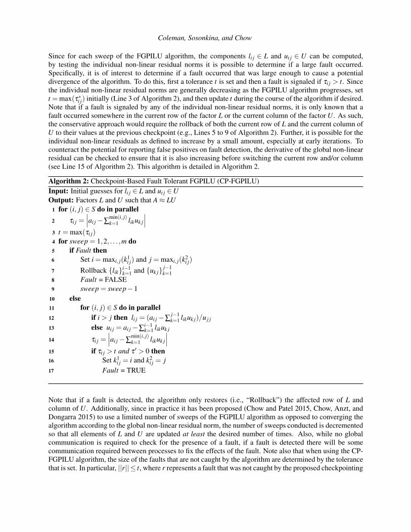
i j) initially (Line 3 of Algorithm 2), and then update t during the course of the algorithm if desired.Note that if a fault is signaled by any of the individual non-linear residual norms, it is only known that afault occurred somewhere in the current row of the factor L or the current column of the factor U . As such,the conservative approach would require the rollback of both the current row of L and the current column ofU to their values at the previous checkpoint (e.g., Lines 5 to 9 of Algorithm 2). Further, it is possible for theindividual non-linear residuals as defined to increase by a small amount, especially at early iterations. Tocounteract the potential for reporting false positives on fault detection, the derivative of the global non-linearresidual can be checked to ensure that it is also increasing before switching the current row and/or column(see Line 15 of Algorithm 2). This algorithm is detailed in Algorithm 2.

Algorithm 2: Checkpoint-Based Fault Tolerant FGPILU (CP-FGPILU)Input: Initial guesses for li j ∈ L and ui j ∈UOutput: Factors L and U such that A ≈ LU

1 for (i, j) ∈ S do in parallel2 τi j =

∣∣∣ai j −∑min(i, j)k=1 likuk j

∣∣∣3 t = max(τi j)4 for sweep = 1,2, . . . ,m do5 if Fault then6 Set i = maxi, j(k1

i j) and j = maxi, j(k2i j)

7 Rollback {lik}i−1k=1 and {uk j} j−1

k=18 Fault = FALSE9 sweep = sweep−1

10 else11 for (i, j) ∈ S do in parallel12 if i > j then li j = (ai j −∑

j−1k=1 likuk j)/u j j

13 else ui j = ai j −∑i−1k=1 likuk j

14 τi j =∣∣∣ai j −∑

min(i, j)k=1 likuk j

∣∣∣15 if τi j > t and τ ′ > 0 then16 Set k1

i j = i and k2i j = j

17 Fault = TRUE

Note that if a fault is detected, the algorithm only restores (i.e., “Rollback”) the affected row of L andcolumn of U . Additionally, since in practice it has been proposed (Chow and Patel 2015, Chow, Anzt, andDongarra 2015) to use a limited number of sweeps of the FGPILU algorithm as opposed to converging thealgorithm according to the global non-linear residual norm, the number of sweeps conducted is decrementedso that all elements of L and U are updated at least the desired number of times. Also, while no globalcommunication is required to check for the presence of a fault, if a fault is detected there will be somecommunication required between processes to fix the effects of the fault. Note also that when using the CP-FGPILU algorithm, the size of the faults that are not caught by the algorithm are determined by the tolerancethat is set. In particular, ||r|| ≤ t, where r represents a fault that was not caught by the proposed checkpointing

Coleman, Sosonkina, and Chow

scheme, since if ||r|| > t than the fault would be caught by the check on Line 15 of Algorithm 2. This, inturn, affects the update equations Eqs. (2) and (3).

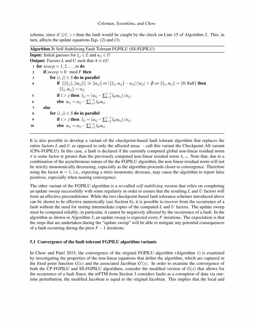
Algorithm 3: Self-Stabilizing Fault Tolerant FGPILU (SS-FGPILU)Input: Initial guesses for li j ∈ L and ui j ∈UOutput: Factors L and U such that A ≈ LU

1 for sweep = 1,2, . . . ,m do2 if sweep ≡ 0 mod F then3 for (i, j) ∈ S do in parallel4 if {∥li j∥,∥ui j∥}≫ ∥ai j∥ or |{li j,ui j}−ai j|/|ai j|> β or {li j,ui j}= {0,NaN} then

{li j,ui j}= ai j

5 if i > j then li j = (ai j −∑j−1k=1 likuk j)/u j j

6 else ui j = ai j −∑i−1k=1 likuk j

7 else8 for (i, j) ∈ S do in parallel9 if i > j then li j = (ai j −∑

j−1k=1 likuk j)/u j j

10 else ui j = ai j −∑i−1k=1 likuk j

It is also possible to develop a variant of the checkpoint-based fault tolerant algorithm that replaces theentire factors L and U as opposed to only the affected areas - call this variant the Checkpoint All variant(CPA-FGPILU). In this case, a fault is declared if the currently computed global non-linear residual normτ is some factor α greater than the previously computed non-linear residual norm τi−1. Note that, due to acombination of the asynchronous nature of the the FGPILU algorithm, the non-linear residual norm will notbe strictly monotonically decreasing, especially as the algorithm proceeds closer to convergence. Thereforeusing the factor α = 1, i.e., expecting a strict monotonic decrease, may cause the algorithm to report falsepositives, especially when nearing convergence.

The other variant of the FGPILU algorithm is a so-called self-stabilizing version that relies on completingan update sweep successfully with some regularity in order to ensure that the resulting L and U factors willform an effective preconditioner. While the two checkpoint-based fault tolerance schemes introduced abovecan be shown to be effective numerically (see Section 6), it is possible to recover from the occurrence of afault without the need for storing intermediate copies of the computed L and U factors. The update sweepmust be computed reliably; in particular, it cannot be negatively affected by the occurrence of a fault. In thealgorithm as shown in Algorithm 3, an update sweep is expected every F iterations. The expectation is thatthe steps that are undertaken during the “update sweep” will be able to mitigate any potential consequencesof a fault occurring during the prior F −1 iterations.

5.1 Convergence of the fault tolerant FGPILU algorithm variants

In Chow and Patel 2015, the convergence of the original FGPILU algorithm (Algorithm 1) is examinedby investigating the properties of the non-linear equations that define the algorithm, which are captured inthe fixed point function G(x) and the associated Jacobian G′(x). In order to examine the convergence ofboth the CP-FGPILU and SS-FGPILU algorithms, consider the modified version of G(x) that allows forthe occurrence of a fault Since, the mFTM from Section 3 considers faults as a corruption of data via one-time perturbation, the modified Jacobian is equal to the original Jacobian. This implies that the local and

Coleman, Sosonkina, and Chow

global convergence results from Chow and Patel 2015 hold for the modified equations that describe the faulttolerant variants of the FGPILU algorithm. Generally, convergence for all of the variants relies on theirproducing the elements in the original domain of the problem (using either checkpointing or a stabilizingstep); as the elements are updated convergence will eventually occur. For the proposed self stabilizingFGPILU, following Theorem 2 from Sao and Vuduc 2013, a result about the convergence may be stated as:

Theorem 1. For any state of li j ∈ L and ui j ∈U, if a correction is performed in the kth sweep, all subsequentiterations are fault-free, no elements in the final L and U factors differ by more than β percent from theoriginal factors in the matrix A, and β is chosen such that if a fault occurs a fault is signaled, then theSS-FGPILU algorithm will converge.

Proof. This follows from noticing that the correcting (or “stabilizing”) step (Lines 2 to 6 of Algorithm 3)ensures that the state li j ∈ L and ui j ∈ U of the incomplete L and U factors will be in the original domainof the problem and then invoking the convergence arguments for the original FGPILU algorithm (see Chowand Patel 2015) which rely upon the assumptions and base arguments from Frommer and Szyld 2000.

Note that finding an appropriate value for the the constant β may be difficult in practice in situations whereapproximate L and U factors cannot be determined by alternative means. The theorem only guarantees thatif such parameters exist and can be found that the algorithm will converge successfully. The convergence ofthe checkpoint-based variants of the FGPILU variants follows directly from the convergence of the originalFGPILU algorithm. Assuming that faults do not occur after a certain number of sweeps, the algorithm willconverge under the assumption that it was successfully returned to a state not affected by a fault. Note that ifa fault is detected, the state is restored to the last known good state - how recent that state is depends on thefrequency with which the checkpoint is stored. More frequent storage of a “good” state via checkpointingwill slow down the overall progression of the algorithm, but will provide a more recent fail-safe state if afault is detected.

Finally, note that for all variants of the FGPILU algorithm if a fault occurs that is not caught by either thestabilizing step in Algorithm 3, or by the checkpointing step in Algorithm 2 it is possible for the Jacobian tomove to a regime where the fixed point mapping that represents the FGPILU algorithm is no longer a con-traction. In this case, the fault tolerance mechanisms of the FPGILU variants will not help, and subsequentiterations of the algorithm will not aid in convergence. Since the application of the FGPILU preconditioneris effectively only an approximate application of the conventional, fault-free ILU preconditioner, the appli-cation of the generated preconditioners can be expressed as, z̃ j ≈ P−1v j. Both Chow and Patel 2015, Chow,Anzt, and Dongarra 2015 have shown that it is possible to successfully use the incomplete LU factoriza-tion resulting from the FGPILU algorithm before the algorithm has converged according to the progress ofthe non-linear residual. It is possible that any adverse affects that a fault may have on the convergence ofthe FGPILU generated incomplete LU factors will not have a meaningful impact on the convergence of theoverarching iterative method (e.g. CG, GMRES, etc). This impact will be explored numerically in Section 6.

6 NUMERICAL RESULTS

The experimental setup for this study is an NVIDIA Tesla K40m GPU on the Turing High PerformanceCluster at Old Dominion University. The nominal, fault-free iterative incomplete factorization algorithmsand iterative solvers were taken from the MAGMA open-source software library (Innovative Computing Lab2015). All of the results provided in this study reflect double precision, real arithmetic. The test matricesthat were used predominantly come from the University of Florida sparse matrix collection maintained byTim Davis (Davis 1994), and the matrices selected for this study are the same as the ones that were selectedfor the study (Chow, Anzt, and Dongarra 2015) that detailed the performance of the FGPILU algorithm on

Coleman, Sosonkina, and Chow

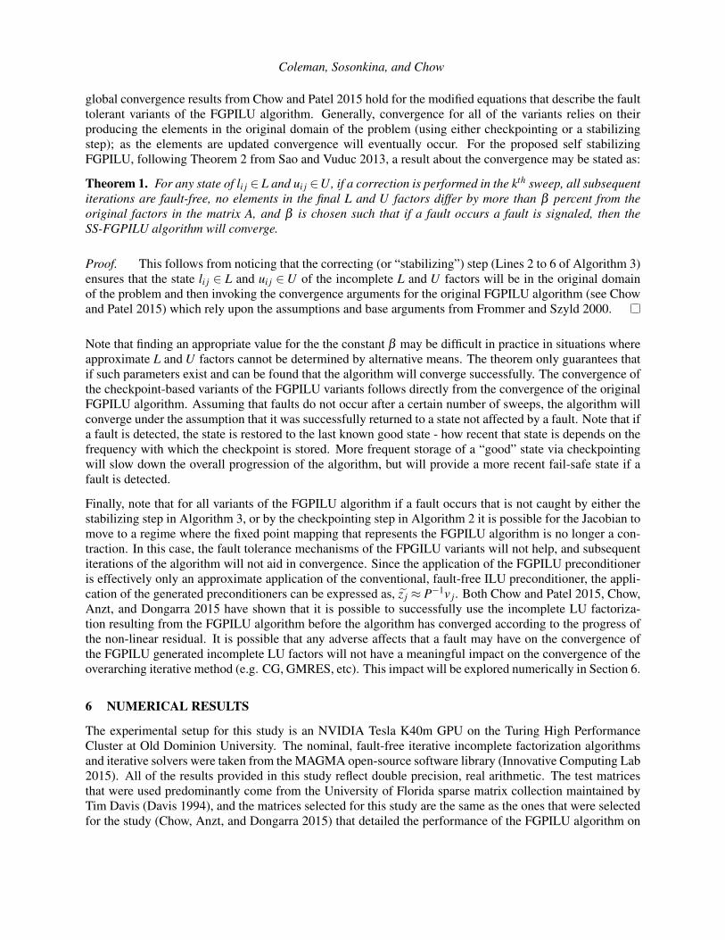
GPUs without the presence of faults. There are six matrices selected from the University of Florida sparsematrix collection, and mimicking the approach in Chow, Anzt, and Dongarra 2015, all six of these matriceswere reordered using the Reverse Cuthill-McKee (RCM) ordering in an effort to decrease the bandwidthand help to improve convergence. The two other test matrices that were used come from the finite differencediscretization of the Laplacian in both 2 and 3 dimensions with Dirichlet boundary conditions. For the 2Dcase, a 5-point stencil was used on a 500×500 mesh, while for the 3D case, a 27-point stencil was used on a50×50×50 mesh. All of the matrices considered in this study are symmetric positive-definite (SPD) and assuch the symmetric version of the FGPILU algorithm (i.e. the incomplete Cholesky factorization) was used.Also, recall from Section 4 that each of the eight matrices used in this study will be symmetrically scaled tohave a unit diagonal in order to help improve the performance of the FGPILU algorithm. A summary of allof the matrices that were tested is provided in Table 1.

Table 1: Summary of the 8 symmetric positive-definite matrices used in this study

Matrix Name Abbreviation Dimension Number of Non-zerosAPACHE2 APA 715,176 4,817,870

ECOLOGY2 ECO 999,999 4,995,991G3_CIRCUIT G3 1,585,478 7,660,826OFFSHORE OFF 259,789 4,242,673

PARABOLIC_FEM PAR 525,825 3,674,625THERMAL2 THE 1,228,045 8,580,313LAPLACE2D L2D 250,000 1,248,000LAPLACE3D L3D 125,000 3,329,698

The experiments are divided into two sets. This first set of experiments focuses on the convergence ofthe FGPILU algorithm despite the occurrence of faults and features comparisons of the L and U factorsproduced by the preconditioning algorithms. Faults are injected into the FGPILU algorithm following themethodology described in Section 3. Due to the relatively short execution time of the FGPILU algorithmon the given test problems, a fault is induced only once during each run, at a random sweep number beforeconvergence. Three fault-size ranges were considered: ri ∈ (−0.01,0.01), ri ∈ (−1,1), and ri ∈ (−100,100).Results for the three ranges are averaged and presented in Section 6.1. The second set of experimentsshows the impact of using in a Krylov subspace solver the preconditioners obtained from the first set ofexperiments. Note that in all of the experiments conducted, the condition u j j = 0 was never encountered.Since all the test matrices are SPD, the preconditioning algorithms are Incomplete Cholesky variants, andthe the solver is the preconditioned conjugate gradient (PCG), as implemented in the MAGMA library.

6.1 Convergence of FGPILU algorithm

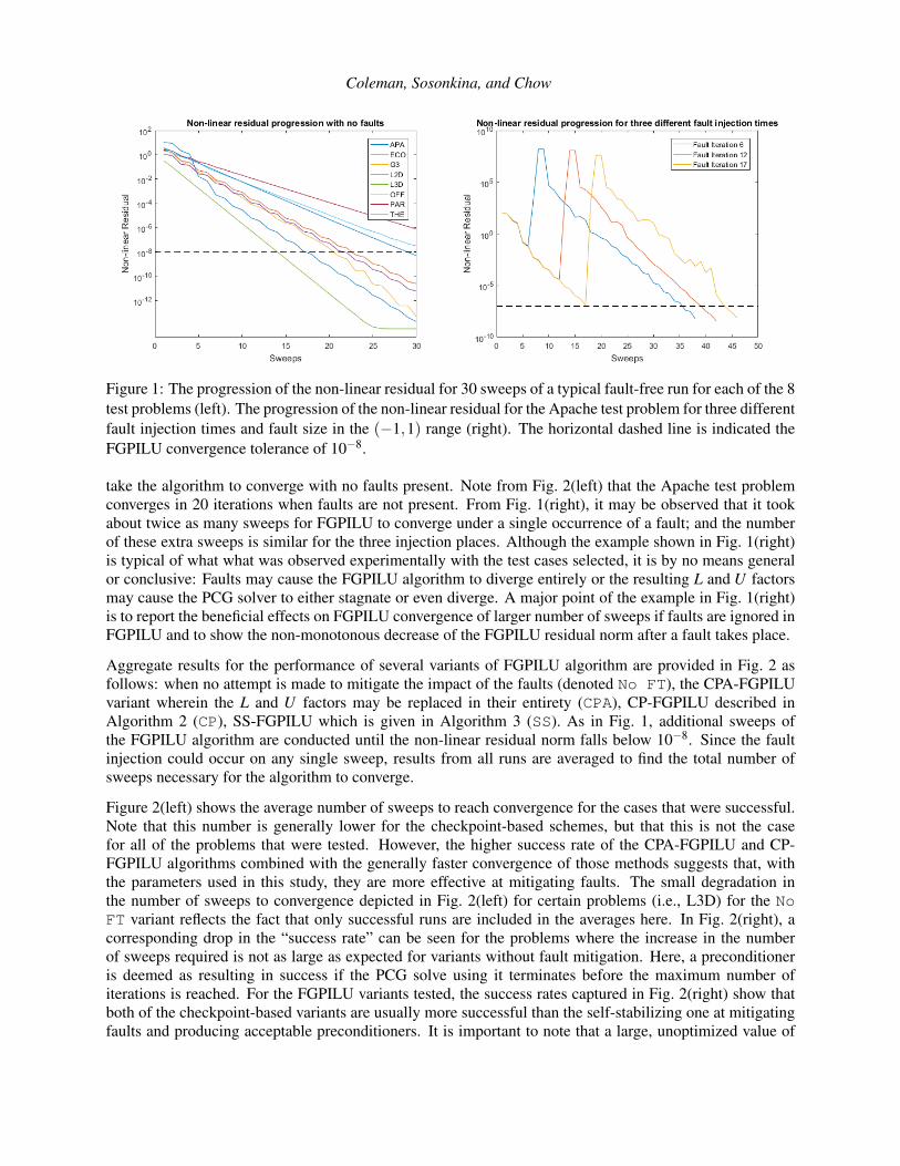
In order to obtain representative results, a fault from each range is injected once, on a single iteration and theresults are averaged over approximately 30–40 runs per problem, all of which are successfully convergedcases. For the purposes of this study, the FGPILU algorithm is said to have converged successfully if thenon-linear residual norm progresses below 10−8. Although this threshold is unnecessarily small from apractical point of view,—it is possible to achieve good performance from a preconditioner with a larger non-linear residual norm—it was chosen so that more sweeps would have to be conducted before the algorithmconverges to better judge the impact of faults. The progression of the non-linear residual norm for a singlefault-free run of each problem is depicted in Fig. 1(left), which is a as an example of the typical progressionof the non-linear residual norm as the algorithm progresses towards convergence.

To illustrate the potential impact of a fault, Fig. 1(right) shows the impact a fault can have on the FGPILUalgorithm when it is injected (and ignored) at the beginning, the middle, or near the end of how long it would

Coleman, Sosonkina, and Chow

Figure 1: The progression of the non-linear residual for 30 sweeps of a typical fault-free run for each of the 8test problems (left). The progression of the non-linear residual for the Apache test problem for three differentfault injection times and fault size in the (−1,1) range (right). The horizontal dashed line is indicated theFGPILU convergence tolerance of 10−8.

take the algorithm to converge with no faults present. Note from Fig. 2(left) that the Apache test problemconverges in 20 iterations when faults are not present. From Fig. 1(right), it may be observed that it tookabout twice as many sweeps for FGPILU to converge under a single occurrence of a fault; and the numberof these extra sweeps is similar for the three injection places. Although the example shown in Fig. 1(right)is typical of what what was observed experimentally with the test cases selected, it is by no means generalor conclusive: Faults may cause the FGPILU algorithm to diverge entirely or the resulting L and U factorsmay cause the PCG solver to either stagnate or even diverge. A major point of the example in Fig. 1(right)is to report the beneficial effects on FGPILU convergence of larger number of sweeps if faults are ignored inFGPILU and to show the non-monotonous decrease of the FGPILU residual norm after a fault takes place.

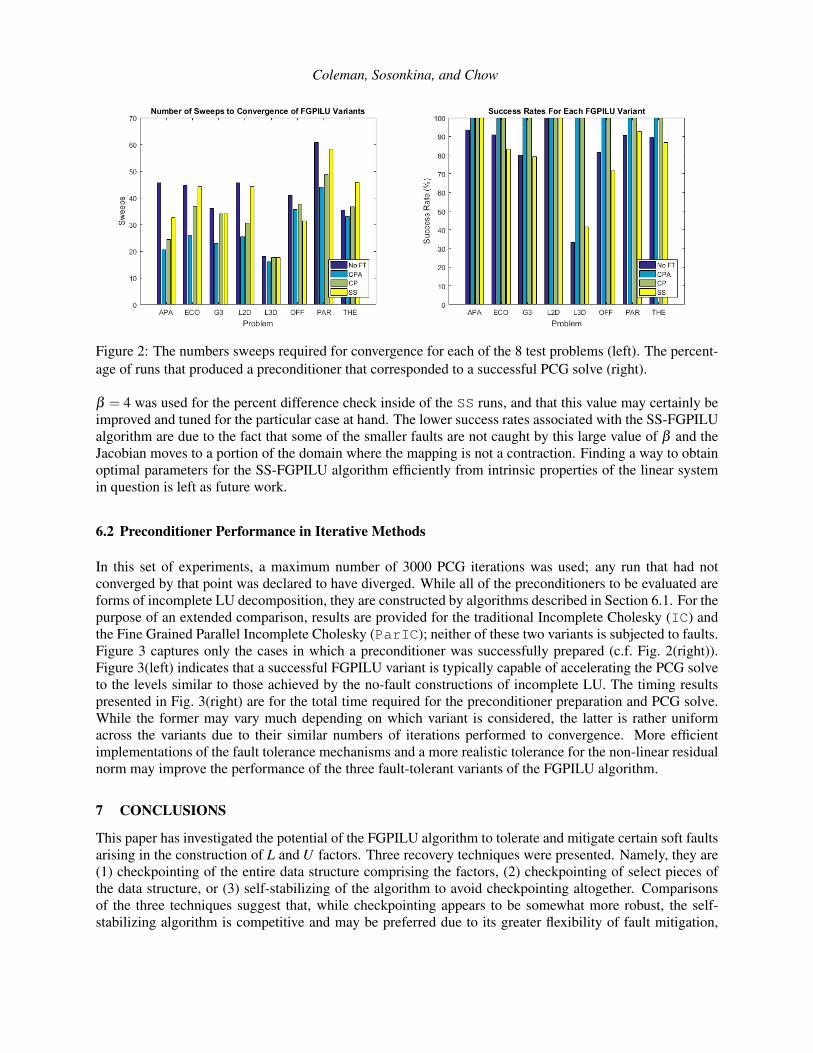
Aggregate results for the performance of several variants of FGPILU algorithm are provided in Fig. 2 asfollows: when no attempt is made to mitigate the impact of the faults (denoted No FT), the CPA-FGPILUvariant wherein the L and U factors may be replaced in their entirety (CPA), CP-FGPILU described inAlgorithm 2 (CP), SS-FGPILU which is given in Algorithm 3 (SS). As in Fig. 1, additional sweeps ofthe FGPILU algorithm are conducted until the non-linear residual norm falls below 10−8. Since the faultinjection could occur on any single sweep, results from all runs are averaged to find the total number ofsweeps necessary for the algorithm to converge.

Figure 2(left) shows the average number of sweeps to reach convergence for the cases that were successful.Note that this number is generally lower for the checkpoint-based schemes, but that this is not the casefor all of the problems that were tested. However, the higher success rate of the CPA-FGPILU and CP-FGPILU algorithms combined with the generally faster convergence of those methods suggests that, withthe parameters used in this study, they are more effective at mitigating faults. The small degradation inthe number of sweeps to convergence depicted in Fig. 2(left) for certain problems (i.e., L3D) for the NoFT variant reflects the fact that only successful runs are included in the averages here. In Fig. 2(right), acorresponding drop in the “success rate” can be seen for the problems where the increase in the numberof sweeps required is not as large as expected for variants without fault mitigation. Here, a preconditioneris deemed as resulting in success if the PCG solve using it terminates before the maximum number ofiterations is reached. For the FGPILU variants tested, the success rates captured in Fig. 2(right) show thatboth of the checkpoint-based variants are usually more successful than the self-stabilizing one at mitigatingfaults and producing acceptable preconditioners. It is important to note that a large, unoptimized value of

Coleman, Sosonkina, and Chow

Figure 2: The numbers sweeps required for convergence for each of the 8 test problems (left). The percent-age of runs that produced a preconditioner that corresponded to a successful PCG solve (right).

β = 4 was used for the percent difference check inside of the SS runs, and that this value may certainly beimproved and tuned for the particular case at hand. The lower success rates associated with the SS-FGPILUalgorithm are due to the fact that some of the smaller faults are not caught by this large value of β and theJacobian moves to a portion of the domain where the mapping is not a contraction. Finding a way to obtainoptimal parameters for the SS-FGPILU algorithm efficiently from intrinsic properties of the linear systemin question is left as future work.

6.2 Preconditioner Performance in Iterative Methods

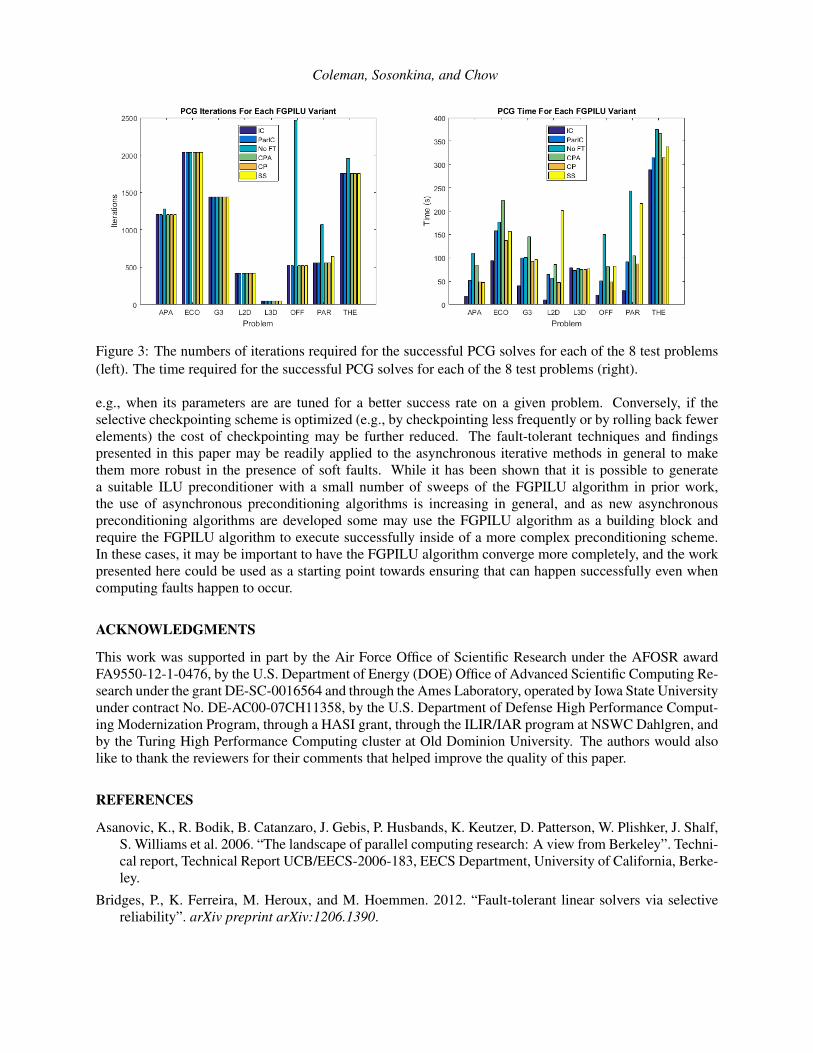
In this set of experiments, a maximum number of 3000 PCG iterations was used; any run that had notconverged by that point was declared to have diverged. While all of the preconditioners to be evaluated areforms of incomplete LU decomposition, they are constructed by algorithms described in Section 6.1. For thepurpose of an extended comparison, results are provided for the traditional Incomplete Cholesky (IC) andthe Fine Grained Parallel Incomplete Cholesky (ParIC); neither of these two variants is subjected to faults.Figure 3 captures only the cases in which a preconditioner was successfully prepared (c.f. Fig. 2(right)).Figure 3(left) indicates that a successful FGPILU variant is typically capable of accelerating the PCG solveto the levels similar to those achieved by the no-fault constructions of incomplete LU. The timing resultspresented in Fig. 3(right) are for the total time required for the preconditioner preparation and PCG solve.While the former may vary much depending on which variant is considered, the latter is rather uniformacross the variants due to their similar numbers of iterations performed to convergence. More efficientimplementations of the fault tolerance mechanisms and a more realistic tolerance for the non-linear residualnorm may improve the performance of the three fault-tolerant variants of the FGPILU algorithm.

7 CONCLUSIONS

This paper has investigated the potential of the FGPILU algorithm to tolerate and mitigate certain soft faultsarising in the construction of L and U factors. Three recovery techniques were presented. Namely, they are(1) checkpointing of the entire data structure comprising the factors, (2) checkpointing of select pieces ofthe data structure, or (3) self-stabilizing of the algorithm to avoid checkpointing altogether. Comparisonsof the three techniques suggest that, while checkpointing appears to be somewhat more robust, the self-stabilizing algorithm is competitive and may be preferred due to its greater flexibility of fault mitigation,

Coleman, Sosonkina, and Chow

Figure 3: The numbers of iterations required for the successful PCG solves for each of the 8 test problems(left). The time required for the successful PCG solves for each of the 8 test problems (right).

e.g., when its parameters are are tuned for a better success rate on a given problem. Conversely, if theselective checkpointing scheme is optimized (e.g., by checkpointing less frequently or by rolling back fewerelements) the cost of checkpointing may be further reduced. The fault-tolerant techniques and findingspresented in this paper may be readily applied to the asynchronous iterative methods in general to makethem more robust in the presence of soft faults. While it has been shown that it is possible to generatea suitable ILU preconditioner with a small number of sweeps of the FGPILU algorithm in prior work,the use of asynchronous preconditioning algorithms is increasing in general, and as new asynchronouspreconditioning algorithms are developed some may use the FGPILU algorithm as a building block andrequire the FGPILU algorithm to execute successfully inside of a more complex preconditioning scheme.In these cases, it may be important to have the FGPILU algorithm converge more completely, and the workpresented here could be used as a starting point towards ensuring that can happen successfully even whencomputing faults happen to occur.

ACKNOWLEDGMENTS

This work was supported in part by the Air Force Office of Scientific Research under the AFOSR awardFA9550-12-1-0476, by the U.S. Department of Energy (DOE) Office of Advanced Scientific Computing Re-search under the grant DE-SC-0016564 and through the Ames Laboratory, operated by Iowa State Universityunder contract No. DE-AC00-07CH11358, by the U.S. Department of Defense High Performance Comput-ing Modernization Program, through a HASI grant, through the ILIR/IAR program at NSWC Dahlgren, andby the Turing High Performance Computing cluster at Old Dominion University. The authors would alsolike to thank the reviewers for their comments that helped improve the quality of this paper.

REFERENCES

Asanovic, K., R. Bodik, B. Catanzaro, J. Gebis, P. Husbands, K. Keutzer, D. Patterson, W. Plishker, J. Shalf,S. Williams et al. 2006. “The landscape of parallel computing research: A view from Berkeley”. Techni-cal report, Technical Report UCB/EECS-2006-183, EECS Department, University of California, Berke-ley.

Bridges, P., K. Ferreira, M. Heroux, and M. Hoemmen. 2012. “Fault-tolerant linear solvers via selectivereliability”. arXiv preprint arXiv:1206.1390.

Coleman, Sosonkina, and Chow

Bronevetsky, G., and B. de Supinski. 2008. “Soft error vulnerability of iterative linear algebra methods”. InProceedings of the 22nd annual international conference on Supercomputing, pp. 155–164. ACM.

Cappello, F., A. Geist, W. Gropp, S. Kale, B. Kramer, and M. Snir. 2014. “Toward exascale resilience: 2014update”. Supercomputing frontiers and innovations vol. 1 (1).

Chow, E., H. Anzt, and J. Dongarra. 2015. “Asynchronous iterative algorithm for computing incompletefactorizations on GPUs”. In International Conference on High Performance Computing, pp. 1–16.Springer.

Chow, E., and A. Patel. 2015. “Fine-grained parallel incomplete LU factorization”. SIAM Journal on Scien-tific Computing vol. 37 (2), pp. C169–C193.

Coleman, E., and M. Sosonkina. 2016a. “A Comparison and Analysis of Soft-Fault Error Models usingFGMRES”. In Proceedings of the 6th annual Virginia Modeling, Simulation, and Analysis Center Cap-stone Conference. Virginia Modeling, Simulation, and Analysis Center.

Coleman, E., and M. Sosonkina. 2016b. “Evaluating a Persistent Soft Fault Model on Preconditioned Itera-tive Methods”. In Proceedings of the 22nd annual International Conference on Parallel and DistributedProcessing Techniques and Applications.

Davis, TA 1994. “The University of Florida Sparse Matrix Collection”. http://www.cise.ufl.edu/research/sparse/matrices/.

Elliott, J., M. Hoemmen, and F. Mueller. 2015. “A Numerical Soft Fault Model for Iterative Linear Solvers”.In Proceedings of the 24nd International Symposium on High-Performance Parallel and DistributedComputing.

Frommer, A., and D. Szyld. 2000. “On asynchronous iterations”. Journal of computational and appliedmathematics vol. 123 (1), pp. 201–216.

Geist, A., and R. Lucas. 2009. “Major computer science challenges at exascale”. International Journal ofHigh Performance Computing Applications.

Innovative Computing Lab 2015. “Software distribution of MAGMA”. http://icl.cs.utk.edu/magma/.

Saad, Y. 2003. Iterative methods for sparse linear systems. Siam.

Sao, P., and R. Vuduc. 2013. “Self-stabilizing iterative solvers”. In Proceedings of the Workshop on LatestAdvances in Scalable Algorithms for Large-Scale Systems, pp. 4. ACM.

Snir, M., R. Wisniewski, J. Abraham, S. Adve, S. Bagchi, P. Balaji, J. Belak, P. Bose, F. Cappello, B. Carlsonet al. 2014. “Addressing failures in exascale computing”. International Journal of High PerformanceComputing Applications.

AUTHOR BIOGRAPHIES

EVAN COLEMAN is a scientist with the Naval Surface Warfare Center Dahlgren Division. He holds anMS in Mathematics from Syracuse University and is working on a PhD in Modeling and Simulation fromOld Dominion University. His email address is ecole028@odu.edu.

MASHA SOSONKINA is a Professor of Modeling, Simulation and Visualization Engineering at Old Do-minion University. Her research interests include high-performance computing, large-scale simulations,parallel numerical algorithms, and performance analysis. Her email address is msosonki@odu.edu.

EDMOND CHOW is an Associate Professor in the School of Computational Science and Engineering atGeorgia Institute of Technology. His research interests are in numerical methods and high-performancecomputing for solving large-scale scientific computing problems. His email is echow@cc.gatech.edu.