FAST ALGORITHMS FOR DISTANCE-BASED SPATIAL … · Fast Algorithms for Distance-based Spatial...

FAST ALGORITHMS FOR DISTANCE-BASED SPATIAL QUERIES

A thesis submitted in confomiity with the requirements for the degree of Master of Science

Graduate Department of Cornputer Science University of Toronto

Copyright O 2001 by Jingjing Lu

National Library I * m of Canada Bibliothèque nationale du Canada

Acquisitions and Acquisitions et Bibliographie Services services bibliographiques 395 WeUington Street 395, rue Wellingtaci Ottawa ON KI A ON4 OttawaON KtAON4 Canada Canada

Y w N I vmm-

dur U. Nlae rdillrriu

The author has granted a non- exclusive Ycence dowing the National Library of Canada to reproduce, loan, distribute or sell copies of this thesis in microform, paper or electronic formats.

The author retains ownership of the copyright in this thesis. Neither the thesis nor substantial extracts kom it may be printed or othedse reproduced without the author's permission.

L'auteur a accordé une licence non exclusive permettant à la Bibliothèque nationale du Cmada de reproduire, prêter, distribuer ou vendre des copies de cette thèse sous la forme de microfiche/film, de reproduction sur papier ou sur format électronique.

L'auteur conserve la propriété du droit d'auteur qui protège cette thèse. Ni la thèse ni des extraits substantiels de celle-ci ne doivent être imprimés ou autrement reproduits sans son autorisation.

Abstract

Fast Algorithms for Distance-based Spatial Queries

Iingjing Lu

Master of Science

Graduate Department of Cornputer Science

University of Toronto

200 1

Spatial databases can be used in many computing-related disciplines to represent

objects in multi-dimensional spaces. One important type of query in such systems

involves retneving ail objects within a specified distance of a specified query point. In

sorne cases, the answers to such quenes are more usehl if they are presented to the user

with objects ordered by increasing distance fiom the query point.

in this thesis, we propose two algorithms for answering the Sphere Intersection Query

(SIQ) and the Distance Query (DQ). SIQ is a special case of the Range Query where the

query window is a sphere instead of an iso-oriented rectangle. Our DQ algorithm is

incremental in the sense that objects are reported one by one in ascending order of

distance. This way, a query processor can use the algorithm in a pipeline fashion for

complex queries. Both of these two algorithms make use of the Filrer Tree, a hierarchical

spatial data structure, as an index.

The performance of each of the two algorithms is evaluated through both analysis and

experimentation with a prototype implementation. Experiments are performed using

datasets consisting of both points and line segments.

Acknowledgements

1 wodd like to extend my sincere gratitude to my supervisor Professor Kenneth

Sevcik. I deem it a great pleasure to have the opportunity to work with Ken. 1 have

leamed a lot fiom his clarity of thought, his consistence and his charming personality.

Without his brilliant insights and strict analysis, I would never bring this project to

fruition. He is a true mentor.

I wouid also like to thank my second reader Professor Renee Miller, thank her for her

precious tirne and highly vaiued comments.

As a personal achievement, 1 dedicate this thesis to my dear parents. They have s h o w

me the power of having a spirit of generosity and unconditional love. Their continuous

support and encouragement have always been my impetus to accomplish my next goal in

life. Al1 1 have accomplished and I will ever be 1 owe to my loving mother and father.

1 also am gratefd to my friends at University of Toronto, thank al1 of them for sharing

the cherishable graduate life with me. Especially, 1 would like to thank George

Giakkoupis. George, highly intelligent, can aiways come up with a better solution to the

question that 1 have struggled for days. Brett Kennedy provides me with a lot of highly

insightful suggestions and help at the beginning of this project.

Last, but not the least, 1 would thank Cara for her moral support.

iii

Contents

1 . INTRODUCTION ......................................................................................................... 1

2 . RELATED WORK .....b.....b............~~............................................................................. 7

2.1 INCREMENTAL ALGORITHMS TO (K-) NEAREST NEIGHBOR QUERIES ..... .................... 7

2.1.1 The k-d Tree and Broder S Algorithm ................................................................ 7

2.1.2 The LSD-Tree and Henrich 's Algorithm ............................................................ 8

2.1.3 PMR Quadtree and Hjaltason & Samet 's Algorithm ........................................ 9

2.1.4 R-Tree Fami& ............................................................................................. 10

2.1.4.1 R-Tree ..................................................................................................... 10

2.1 .4.2 ~ + - ~ r e e ..................................................................................................... 1 1

2.1.4.2 R*-Tree ..................................................................................................... 12

2.2 OVERVIEW OF THE FILTER TREE .............................................................................. 13

2.2.1 Range Queries ................................................................................................ I S

2.2.2 Spatial Join Queries ......................................................................................... 17

3 . PROBLEM STATEMENT ........................................................................................ 19

3.1 MOTIVATION ............................................................................................................ 19

3.2 CRITEU FOR EFFICIENCY ....................................................................................... 20

3.3 SPHERE INTERSECTION QUERY AND DISTANCE QUERY ........................................... 2 1

3.3.1 Sphere Intersection Queries ............................................................................. 22

3.3.2 Distance Queries .......................................................................................... 23

3.4 ACCURACY M DISTANCE CALCULATION ................................................................. 25

3.4 l Dis fance for MBRF w itho ut Slope .................................................................... 25

3.4 1 Distance for MBRr with Slope ......................................................................... 26

4 . EXPERIMENTAL SETUP ...................................................................................... 29

.......................................................... 4.1 THE QUESTIONS AND ANTICIPATED RESULTS 29

4.2 SYNTHETIC DATA USED ........................................................................................... 29

4.3 REAL DATA USED .............................................................................................. 31

4.4 QUERY WINWWS USED ......................................................................................... 35

5 . EXPERIMENTAL RESULTS: SPHERE INTERSECTION QUERY ...... .. ......... 37

5.1 EXPERIMENTS 1 AND 2: VARYMG THE SIZE OF THE DATASET ................................. 37

................................. 5.2 EXPERIMENTS 3 AND 4: VARY MG THE QUERY WINDOW SIZE 45

5.3 EXPERIMENTS 5 AND 6: VARYMG THE QUERY WINDOW POSITION ......................... 50

5.4 EXPERIMENTS SUMMARY ......................................................................................... 53

6 . EXPERIMENTAL RESULTS: DISTANCE QUERY .... .. .................................. 54

6.1 EXPER~MENTS 1 AND 2: VARY~NG THE SIZE OF THE DATASET ................................. 55

6.2 EXPERIMENTS 3 AND 4: VARYMG THE QUERY WINDOW SIZE ................................. 57

.................................. 6.3 EXPERIMENTS 5 AND 6: VARYMG THE SIZE OF SORTED LIST 60

......................................................................................... 6.4 EXPERIMENTS SLJMMARY 65

7. CONCLUSIONS AND FUTURE WORK..... ........................................................... 66

.......................................................................................................... 7.1 CONCLUS t o ~ s 66

7.2 FUTURE WORK ......................................................................................................... 67

7.2.1 Data with Higher Dimenrionality .................................................................... 67

7.2.2 Distance Join and Semi-Distance Join ............................................................ 67

APPENDIX A .................................................................................................................. 72

APPENDIX B .................................................................................................................. 75

Chapter 1

Introduction

With an increasing nurnber of computer applications that rely heavily on spatial data,

more and more attention has been devoted to spatial data management. Besides the

original applications, like cartography, mechanical CAD and GIS (Geographic

Information System), nowadays spatial data are heavily used in the areas such as

robotics, visual perception, environmentai and medicai imaging. A great variety of spatial

access rnethods have been proposed in the past two decades to make the access to the

spatial data more efficient.

1.1 Spatial Data

Spatial data is the data that describes the space and its embedded objects including

points, lines, areas and volumes. Generally, we assume that the given objects are

embedded in d-dimensionai Euclidean space Ed or a suitable subspace thereof. Since

indices o h perform m m effÏciendy whni handlhg simple entries of a consistent fom,

we often abstract a simpler shape nom the actual shape of a spatial object before

inserthg it into an index. For example, in a city geographic database, buildings may be

stored as points; riven and roads can be stored as a set of line segments; and parking lots,

playgrounds and water areas can be stored as minimum bounding rectangles (MBRYs),

the mallest rectangles that are aligned with the axes of the two-dimensionai space and

enclose the entities' shapes. An index is defined to administrate the simplified shape of

each object while a pointer to the achial object database is maintained.

Differem techniques are used to represent the spatiaf data. For exampie: an MBR c m

be specified either by the coordinates of the lower left comer and the upper right comer,

or by the coordinate of the centroid of the MBR and the extent in each dimension.

1.2 Spatial Queries

Spatial queries are queries against one or more spatial datasets. Since there is neither

standard algebra nor a standard spatial query laquage defined on spatial data, we will

have to define severai commonly used spatial database operators, which will be

addressed in this thesis,

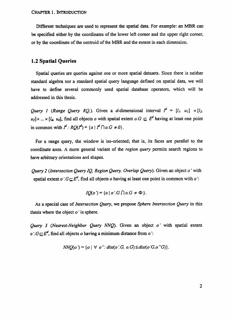
Quev I (Range Query RQ,). Given a d-dimensional interval f = [I l , u,] x [12#

UZ] x ... x [Id ud], find ail objects O with spatial extent o.G c lid having at least one point

incornmon withf: RQ(P)= ( O P f l o . ~ + O } .

For a range query, the window is iso-oriented; that is, its faces are parallel to the

coordinate axes. A more general variant of the region query permits search regions to

have arbitras) orientations and shapes.

Query 2 (Intersection Query IQr Region Query, Overlap Query). Given an object O ' with

spatial extent O '. G Ed, find al1 objects o having at least one point in common with O ':

As a special case of Intersection Q z i q we propose Sphere I ~ s e c t i u n pl.y in this

thesis where the object O ' is sphere.

Query 3 (Nearesi-Neighbor Query m). Given an object O ' with spatial extent

O '. G~ l?, h d dl objects O having a minimum distance from O ':

Query 4 (Distance Query DQ). Given an object o ' with spatial extect O '. G~ p, find up

to the nearest N objects 01, 02.. . ... ON having a distance between [disr,, disi-] fiom O ' in

the ascending order of distance:

DQ(o 7 = (O, 1 V i <]SN: distmin I dist(o '. G, 01. G) S dist(o '. G, O,. G) < dist(o '. G, O,. G)

< dist(o : G, ON. G) s dist-) .

The Nearest-Neighbor Query can be regarded as a special case of Distance Query,

where N (the nurnber of records in the result set) equals 1, and disr,, equais O and disi,,

is unlimited,

The distance between extended spatial data objects is usually defined as either the

distance between the centroids or the distance between the closest points. Cornmon

distance functions for points include the Euclidean and Manhattan distances. In thk

thesis, we will use the distance between the centroids under Euclidean metrics. A

discussion why this distance measure is more appropriate than the distance between the

closest points will be presented in Chapter 3.

Besides spatial selections, as exemplified by Quenes 1 through 4, the spatial join is one

of the most important spatial operations and can be defined as fo1lows [Gunther 19931:

Query 5 (Spatial Juin). Given two collections R and S of spatial objects and spatial

predicate 0 , find ail pa in of objects (o,o 7 E R x S where 0 (0.G. o '. G) evaiuates to true:

RDU OS= {(o,o? 1 OERAO'ESA 0(o.G, 03) ).

The spatial predicate 0 has a wide variety of possible interpretations, including

intersects(*), contaim(.), is-enclosed-bfi.), distance(.) O E { =. S. <, 2, > ) .

1 3 Spatial Access Methods

Spatial access methods (SAMs) are typically based on point access methods (PAMs)

which are designed to handle sets of data points. However, PAMs are not directly

applicable to databases containing objects with a spatial extension. The main problem

when designing the spatial access methods is that there exists no totaI ordering among

spafiaI objects that preserves spatid proximity. In other words, there is no mapping from

two- or higher-dimensional space such that any two objects that are spatially close in the

higher-dimensional space are dways close to each other in the one-dimensional sorted

sequence. Also, the fact that spatial data is usually complex and large and there is no

standard algebra defined on spatial data makes the spatial operations more expensive than

standard relational operations. Al1 these factors make the design of efficient access

methods in the spatial domain more chdlenging than the conventional database.

In order to deai with the specid properties of the extended objects, point access

methods have been modified using the following techniques: Transformation,

Overlapping Regions, Clipping and Multiple Layea [Kriegel et al. 19911. The idea of

Transfomation is to transfomi the objects into a different representation so that one-

dimensional access methods cm be applied to manage spatidly extended objects.

Essentially there are two options: one can either tmnsform each object into a higher-

dimensional point w i ~ c h s 1985; Seeger and Knegel 19881, or transform it into a set of

one-dimensional intervals by means of space-filling curves. The main idea of the

Overlapping Regions technique is to ailow different data buckets in an access method to

correspond to mutudly overlapping subspaces. Typical Overlapping Region methods

include the R-Tree [Gutcman 19841, the R*-Tree [Beckmann et al. 19901, the SKD-Tree

[Ooi et al. 1987; Ooi 19901 and the P-Tree [Jagadish 1 WOc, Schiwiets 19931. in Contrast

to Overlapping Regions, Clipping-based schemes such as the R'-Tree [Stonebraker et al.

1986; Sellis et al. 19871, do not allow any overlaps between bucket regions; they have to

be rnutually disjoint, which means that some objects may have to be represented in more

than one bucket region. The multiple layer technique can be regarded as a variant of the

overlapping regions approach, because data space of the hierarchical layers may overlap,

but the data regions within each layer are disjoint. The Multiloyer Grid File [Six and

Widrnayer 19881 and the R-File [Hutflesz et al. 19901 are the representative methods in

this category.

Besides the spatiai access methods we mentioned above, there are several methods that

take advantage of more than one technique, such as Hilbert R-Tree [Kamel and Faloutsos

19941, which uses both Overlapping Regions and Space-FiIling Cumes; and the Filter

Tree [Sevcik and Koudas 19961, which rnakes a use of a combmation of Mnttipfe Layers

and Space-Filling Curves.

Due to the cornplexity of the data, there are many different cnteria to address quality

and numerous parameten that determine performance. It is almost impossible to expect

one access method to outperfonn ail the competiton in every aspect, since every newly

proposed method is designed to attack some weakness of the previous ones, possibly at

the cost of being iderior with respect to other evaluation criteria.

in this thesis, the terms spatial data, spatial queries and spatial access methods refer to

data, quenes and access methods of two and three dimensions.

This thesis works with the Filter Tree, testing two new queries, Sphere Intersection

Query and Distance Query. In both queries, we wiII have to calculate the distance corn

query center to the cardidate objects to determine if the objects are inside the query

range. As we mentioned previously, the distance Functions are usually based on a

distance meûic for points. However, this is not necessarily dways the case. For example,

we can define the distance fiom a point p to a line 1 as dist @, 2) = min ,,/a 1 dist, (p. pl).

where diStp@, pl) denotes the distance between points p and pl, which is a point on the

line. In this case, the consistency of this distance function is guaranteed by the properties

of dist,, namely, non-negativity and the triangle inequality.

In this thesis, we implement two prototypes based on two different distance functions

under Euclidean metncs: the conventional point to point (PTP) and the point to line

segment (PTLS) metrics. For the PTLS metric, we try to make a more precise

approximation of the line segment. We not only keep the coordinates of the two corners

of the MBR around the line segment, but also the dope of the line. This is under the

assumption that the real object, such as roads and nven will be best represented as a line

between diagonally opposite corners of the MBR. In order to differentiate the line being

either h m the upper right comer to the lower left comer, or h m the upper left comer to

the lower right comer, we use I and -1 to indicate the sign of the slope. The point to line

segment metric will be based on the distance between the center of the query range and

the line segment. We compare the m b e r of V û s , the pmcessor time and the resutt sets

fiom the same input data sets.

1.4 Thesis Organization

The remainder of the thesis is organized as follows:

Chapter 2, Related Work, presents related work in the area of spatial indexing

techniques for new data types. We mainly focus on distance queries and other distance

related operations on other file structures.

Chapter 3, Problem Statement, describes the problem we are going to address in this

thesis. We first compare the two different representations of the spatial data, and then we

state our motivation for the Sphere Intersection Query and Distance Query based on the

two different representations of the data.

Chapter 4, Experimental Setup, explains the data used in the experiments, the position

and the radius used in the Sphere Intersection Query and the Distance Query, the

environment under which we conduct our experiments and a discussion over which data

structure to choose follows.

Chapter 5, Experimental Results for Sphere Intersection Query, presents the

experimentai results on number of VOS and processor time for different datasets. The

anaiysis of the results follows.

Chapter 6, Experirnental Results for Distance Query, provides the results for both VO

costs and processor costs for different datasets. At the end of the chapter, we discuss the

r e d t s that we obtained.

Chapter 7, Conclusions and Future Work, provides a summary of the work done for the

thesis and the significance of the results. It also addresses the possible extensions for this

research in the future-

Chapter 2

Related Work

2.1 Incremental Algorithms for (kg) Nearest Neighbor Queries

Motivated by their relevance to the field of GIS, pattern recognition, learning theory and

image processing, nurnerous algorithms have been proposed to answer nearest neighbor

and k-nearest neighbor quenes. Arnong the algorithms, incremental solutions play an

important role in this literature [Broder 1990; Henrich 1994; Hjaltason and Samet 1995,

19991. Pnority queues are employed in the incremental algorithms for k-d Tree, LSD-

Tree, PMR Quadtree and R-Tree respectively.

2.1.1 The k-d Tree and Broder's Algorithm

A k-d Tree [Bentley 19751 is a binary search tree structure that stores and operates on

records by recursively subdividing the univese into k-dimensionai subspaces using iso-

oriented hyperplanes. Each subspace is represented as a node in the tree containing a

subset of the collection of records. The position of the hyperplane is chosen so that each

of the children contains approximately half of the parent's records.

Broder's algorithm proder 19901 makes use of the k-d Tree as the index structure to

answer the k-nearest neighbor query. It stores oniy the data objects in the priority queue

and takes advantage of a stack to keep track of the subtrees of the spatial data structure

that need to be processed.

This incremental search algorithm contains two functions: search-init and search-next.

The fiuiction semch-inib recursiveiy descends the tree to locate the leaf node that contains

the query point. A Iist of pointers to the non-terminal nodes that were traversed during the

descent is then stored in a stack. Then the search-next function will use the information in

the stack to discover the nearest neighbor to the search point. The distance needs to be

computed between the query point and each of the records contained in the le& node

pointed to by the head of the stack. The pointers to the records become elernents of a

queue, which is ordered by distance to the query center. The record at the head of the

queue is a candidate result for the nearest neighbor and the distance serves as the upper

bound for the distance to the actual nearest neighbor. Al1 the records within the leaf will

be examined to ensure that the first record has the minimum distance to the query point.

Afler that, the tree is ascended one level by popping out the top element fiom the stack.

New candidate records are determined by recursively descending the other child of the

new non-terminal node. This process is repeated until al1 the elements in the stack have

been examined.

2.1.2 The LSD-Tree and Henrich's Algorithm

LSD-Tree [Henrich et al. 19891 is a data structure for multi-dimensionai points, it divides

the data space into painvise disjoint data cells, namely bucket regions. In each bucket

region, a fixed number of objects can be stored. Each time when the threshold for any

region is reached, an attempt to insert an additional object will cause a bucket split. For

this purpose, a split line is detennined through the bucket and the objects are stored in

two buckets according to the split line. This process is repeated whenever the capacity of

a bucket is exceeded.

The split lines of the LSD-Tree are maintained in a directory, which is a generalized k-

d Tree. For each split, a new node containing the position and the dimension of the split

line is Uiserted into the directory tree. The leaves of the directory tree reference the

buckets in which the actual objects are stored.

To answer the Distance Query, the author employs two prionty queues menrich 19941,

OPQ and NPQ, to store objects and directory nodes or buckets. The elements in the

queues are storeci in a way ttiat the me widr the minhm distance to the query c m q

has the highest priority.

The aigorithm starts at the root of the directory and searches for the bucket that

contains q. During each search, if we check the lefi child, the right child will be inserted

into NPQ, else if we follow the right child, the lefi child will be inserted into NPQ. Then

the objects in the conesponding bucket are iwerted into OPQ and a,,. is set to the

minimum distance between q and the closest edge of the searching bucket region.

Thereafter the objects with a distance less than or equal to dm, are taken h m OPQ.

M e r exhausting al1 the elements in OPQ, the search region has to be extended by taking

the top element from NPQ. If it happens to be a directory node, another round of

searching starts. This process repeats until al1 the elements in OPQ and NPQ have been

checked.

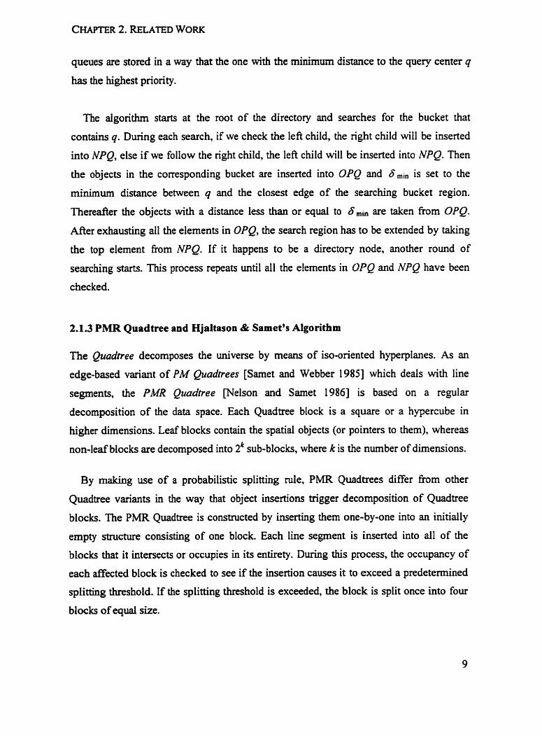
2.1.3 PMR Quadtree and Hjaltason & Samet's Aigorithm

The @&ee decornposes the univene by means of iso-oriented hyperplanes. As an

edge-based variant of PM Quadtrees [Samet and Webber 19851 which deais with line

segments, the PMR Quadtree pelson and Samet 19861 is based on a regular

decornposition of the data space. Each Quadtree block is a square or a hypercube in

higher dimensions. Leaf blocks contain the spatial objects (or pointers to them), whereas

non-leaf blocks are decomposed into sub-blocks, where k is the number of dimensions.

By making use of a probabilistic splitting d e , PMR Quadtrees differ fiom other

Quadtree variants in the way that object insertions trigger decomposition of Quadtree

blocks. The PMR Quadtree is constnicted by inserting them one-by-one into an initially

empty structure consisting of one block. Each line segment is inserted into ail of the

blocks that it intersects or occupies in its entirety. During this process, the occupancy of

each af5ected block is checked to see if the insertion causes it to exceed a predetemined

sptitting threshold. If the splitting threshold is exceeded, the block is split once into four

blocks of equal size.

Tht authors ht~~ducecf a top-dowrr method ~jdtamn a d Samet 19951 to answer the

Distance Query. The algorithm will k t locate the leafnodes containing the query object

q; then a pnority queue is maintained to record the blocks whose descendants have not

been visited as well as the objects that have not yet been visited. The crucial point here is

that, in addition to using the priority queue for containing blocks, objects are also inserted

into the queue as leaf blocks are processed. The key for the priority queue is the distance

fiom the query object to each element, while blocks have higher pnority than objects if

the distances are exactly the sarne. A container is examined only if it reaches the head of

the queue. The objects at the head of the queue (i.e., with shorter distances) are retrieved

until the queue is emptied.

2.1.4 R-Tree Family

R-Trees are an extension of B-Trees for multidirnensional objects that are either points or

regions. Like B-Trees, R-Trees are baianced and guarantee a space utilization of at least

50%. Due to the popularity of R-Trees, Hjaltason and Samet m e r extend their

incremental (k-) nearest neighbor algorithm to the R-Tree and R*-Tree [Hjaltason and

Samet 19991.

An R-Tree [Guttman 1984; Greene 19891 corresponds to a hierarchy of nested d-

dimensional intervals. Each node v of the R-Tree corresponds to a disk page and a d-

dimensional interval f@). If v is an intenor node then the intervais corresponding to the

descendants v, of v are contained in f(v). Intervais at the same tree level may overlap. If v

is a leaf node, f(v) is the d-dimensional minimum bounding rectangle of the objects

stored in v. For each object in tum, v stores only its bfBR and a reference to the complete

object description.

Searching in the R-Tree is similar to searching in the B-Tree. At each index node v, al1

index entries are tested to see whether they intersect the search interval 1,. We should

visit dl child nodes vi with f@Jn I,# O. Due to the possibility of overlapping regions,

there may be several intervals ~ ( V J that satisfy the search predicate. In the worst case,

one may have to visit every index page.

To insert an object O, we insert the minimum bounding interval Id(*) and an object

reference into the tree. In contrast to searching, we traverse only a single path fiom the

root to the leaf. At each level we choose the child node v whose corresponding interval

f ( v ) needs the least enlargement to enclose the data object's interval f(o). If several

intervals satisQ this cnterion, Guttman proposes selecting the descendant associated with

the smallest interval. As a result, we insert the object oniy once; that is, the object is not

dispersed over several buckets. If insertion requires an enlargement of the corresponding

bucket region, we adjust it appropriately and propagate the change upwards.

As for deletion. we fint perform an exact match query for the object. If we find it in

the tree, we delete it. If the bounding intervai can be reduced because of the deletion, we

perform th is adjutment and propagate it upwards.

Many researchea have worked on how to minimize the overlap during insertion. For

exarnple, the packed R-Tree [Roussopoulos and Leifker 19851 cornputes an optimal

partitionhg of the universe and a corresponding minimal R-Tree for a given scenario.

The Hilbert R-Tree [Kamel and Fdoutsos 19941 combines the overlapping regions

technique with space-filling cuves. It fim stores the Hilbert value of the data rectangle's

centroid in a B'-Tree, then enhances each intetior B+-Tree node by the MBR of the

subtree below. This facilitates the insertion of new objects considerably. But since the

splitting policy takes ody the objats' centroids into amunt, the performance of the

structure is likely to deteriorate in the presence of large objects.

R'-Tree [Stonebruker et al. 1986; Sellis et al- 19871 is proposed to overcome the

problems associated with overlapping regions in R-Tree and packed R-Tree. As

mentioned, point searches in ~ + - ~ r e e correspond to single-path tree traversais from the

root to one of the Ieaves. But range searches usually lead to the traversal of multiple paths

in both structures.

When inserting a new object O, we may have to foiIow muItipIe paths, depending on

the number of intersections of the MBR f(o) with index intervals. f (o ) may be split into n

n disjoint hgments l?(o) (U [:(O) = 1-1

leaf node vi. If there is enough space,

intenral f(o) overlaps space that has

intervais corresponding to one or more

Id(o)). Each fragment is then placed in a different

the insertion is straightforward. If the bounding

not yet been covered, we have to enlarge the

leaf nodes. If a Ieaf node overfiows it has to be

split. When splitting, for R'-Tree, the splits rnay propagate not only up the tree, but also

down the tree. This may cause M e r fragmentation of the data intervals. For deletion,

~ ' - ~ r e e fmt locates al1 data nodes where fragments of the object are stored and removes

them. If storage utilization drops below a given threshold, we try to merge the affected

node with its siblings or to reorganize the tree. Though the ~ ' - ~ r e e cannot guarantee

minimum space utilization, the authoa daim that analytical results indicate that R'-~rees

achieve up to 50% savings in disk accesses compared to an R-Tree when searching files

of thousands of rectangles.

The R'TW [Beckmann et of. 19901 is proposed to overcome the weaknesses of the

original algorithms for R-Tree. Since the insertion phase is cntical for good search

performance, the design of the R*-~ree therefore introduces a policy called forced

reinsert: if a node ovediows, it is not split right away, instead p entries are removed From

the node and reinserted in the tree. According to the authors, the parameter should be

about 30% of the maximal number of entries per page. Besides the reinsertion strategy,

Beckmann et al. also rnodified the policy of node-splitting by a plane-sweep paradigrn

[Preparta and Shamos 19851. The goals include minimum overlap between bucket

regions at the same tree level, minimum region perirnetea and maximum storage

utilization. The authors c l a h performance improvements of up to 50% compared to R-

Tree.

CHAPTER 2. RELATED WORK

The paper by Berchtoici et ai. [I 9961 suggests a modification of the R-Tree caited the

X-Tree. The X-Tree introduces supernodes, nodes that are larger than the usual block

size, to reduce overlap arnong directory intervals.

2.2 Ovewiew of the Filter Tree

The Filter Tree can be viewed as a file organization that simultaneously uses hierarchicai

representation, size separation and space-filling curves techniques. By combining these

techniques, Filter Trees can perform spatial joins with a guaranteed minimal number of

biock reads fi-om disk.

In a Filter Tree for a two-dimensional space, the storage of an entity and the access to

it is completely based on its MBR. For concreteness, we refer to the two dimensions as x

and y for the rest of Our discussion, although their interpretation in specific cases will

depend on the application. The Minimum Bounding Rectangle is specified by the

coordinates of its lower left corner (xb y/) and upper right corner (xh yh), where n, xh

(respectively, y, and yh) are the smallest and largest values of the x (respectively y)

coordinate.

Filter Trees achieve the hierarchical representation by a recursive binary partition of

the data space in each dimension. The Filter Tree represents the data space in multiple

levels, where each level divides the data space into a higher number of cells than the

previous level. At level j, the data space is divided into Y subsquares by the partition

lines at k / Y, k = 0, 2, 4 ..., 2' in both x and y dimensions. The irnplementation of the

Filter Tree studied in this thesis uses up to twenty levels, numbered O through 19. Figure

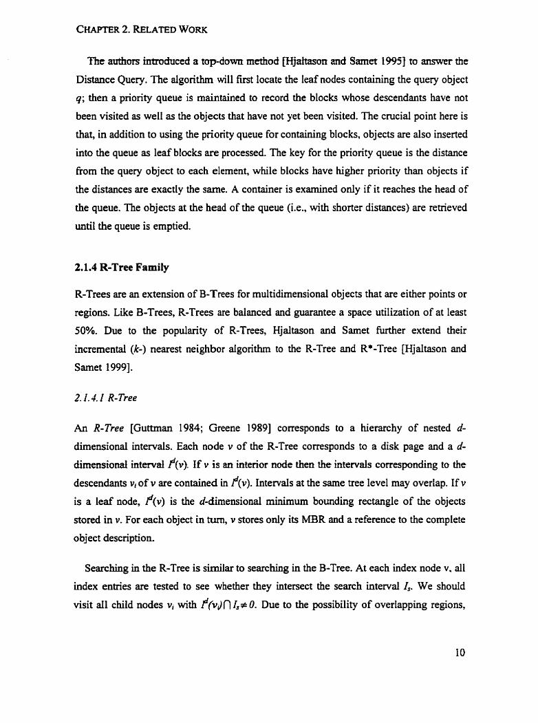
2.1 shows the hierarchical gxids for the first 3 levels.

Each entity to be stored in the Filter Tree is associated with the lowest level (largest

level number) at which the object can entirely reside within a single cell. If an MBR has

one side of length greater than 2', then it will be associated with a level no lower than j.

This way, the relatively large rectangles are guaranteed to be associated with higher

levels in the tree, and relatively small rectangles tend to be associated with lower levels.

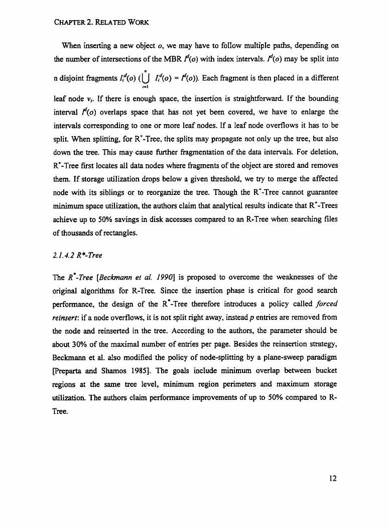
Figure 2.2 illustrates three objects that are stored in the data space. Object A is large and

resides at level 1 of the Filter Tree. Object B is much smaller, and fits within a 118 by 118

cell, so it is associated with level 3 of the tree. Though object C is even smaller, it

happens to straddle grid line x = %, which forces it to be associated with level O of the

tree.

Level O

Level 1

Figure 2.1 Hierarehical Representation of Data Space: Level O to 3

Figure 2.2 Tbree Objects Are Stored in the Filter Tree

Physicai storage of both MBK's and entity records requires a total nurnenc ordering of

the entities. A Hilbert curve is used to obtain this serialized order whiie retaining locality

of overlapping and neighboring entities. The Hilbert curve orders the cells in such a way

that cells that are physically close in the data space will have a high likelihood of being

located near each other on the Hilbert curve. At al1 the levels except level 0, the Hilbert

curve begins in the lower-left corner and ends in the lower-nght corner, and each ce11 is

ordered by its position on the curve. The Hilbert cume visits every ce11 of the level

exactly once, and never crosses itself. Figure 2.3 shows the Hilbert curves for Levels 1

and 2 in two-dimension space. Level O has only a single cell, which is given Hilbert value

O. Objects are given the Hilbert value of the ceil in which they are contained. For

example, in Figure 2.2, object A at Level 1 is associated with Hilbert value 3, object B at

level 3 with Hilbert value 23 and object C at level V with Hilbert value O. Hilbert values

may also be specified as binary fiactions of at least 2k bits, where k is the nurnber of the

levels.

Level O Level 1 Level2

Figure 2.3 Hilbert Cumes at Levels O, 1 and 2

23.1 Range Queries

Given a query window specified by its lower left and upper right point coordinates, we

expect to retrieve al1 entities in the tree that overlap the window. At any given level, the

query window will cover certain ranges of Hilbert values. This set of ranges of Hilbert

values is first cdculated at one level of the Filter Tree, known as the containment level.

Figure 2 . 4 ~ illustrates an exarnple of a query window where Level 2 is used as the

containment level. In this case, the window covers the Hilbert ranges: 4 to 7.

Figure 2.4 Query Window at Level O, 1,2 and 3 of the Filter Tree

Once the ranges of Hilbert vaiues that the window covers at the containment IeveI are

found, it is simple to caiculate the Hilbert values at al1 other levels. For example, each

ce11 at the containment level covers at most four cells at the level below. These four cells

c m be found by rnultiplying the Hilbert value at the containment ievel by four, and the

adding zero, one, two and three. For example, Ce11 1 at Level 1 corresponds to Cells 4, 5,

6 and 7 at Level 2. So, in the case above, the ranges of Hilbert values covered by the

window is 4 to 7 at Level2. We can calculate that the window covers a subset of Cells 16

to 3 1 at Level3. Figure 2.4d shows us that the window covers 18,23 to 24 and 27 to 29.

A simifar method can be usect to fmd the ceils two tevels down. This invobes muItip1ying

by 16, then adding O to 15 and so forth.

To find the corresponding cells at higher levels, we instead divide by four and then

apply the floor function. For exarnple, in the case above, the range 4 to 7 at Level 2

corresponds to Cells 1 ai Level 1 and Ce11 O at Level O. Figure 2.4b and Figure 2.4a

illustrate this.

When the ranges of Hilbert values are calculated for each Ievel, the data files of the

Filter Tree are processed one level at a tirne. For each Ievel, the index file is exarnined to

determine which data pages must be read. The required data pages are read and each

object is compared with the query window. A buffer is used to store both index and data

pages.

2.2.2 Spatial Join Queries

The join operation is one of the most cornmonly w d ways to combine information fkom

two or more relations. Spatial join retrieves d l object pairs that satisQ a spatial predicate

on objects fiom two or more datasets.

Spatial join operations are performed in two steps. The first step, namely the filter step;

retrieves a Iist of candidate pairs by applying the query predicate on an approximate

representation, such as the MBR. The next step, called the refinement step, tests the full

predicate against the actual spatial objects identified in the filter step. The first step is

more critical mice the purpose is to n m w the search range of the refmement step, m

order to reduce the number of entity records that mus& be read fiom disk.

A spatial join between two Filter Trees involves an index sweeping process. However,

the structure of the Filter Tree makes the sweeping process very efficient. For any pair of

data sets, their hill spatial join can be cornputed with the minimal amount of VO, namely

by reading each block of the entity descnptor file exactly once. This is accomplished by

sweeping concurrently through the entity descriptor files for level of each participating

Filter Tree in increasing Hilbert value order.

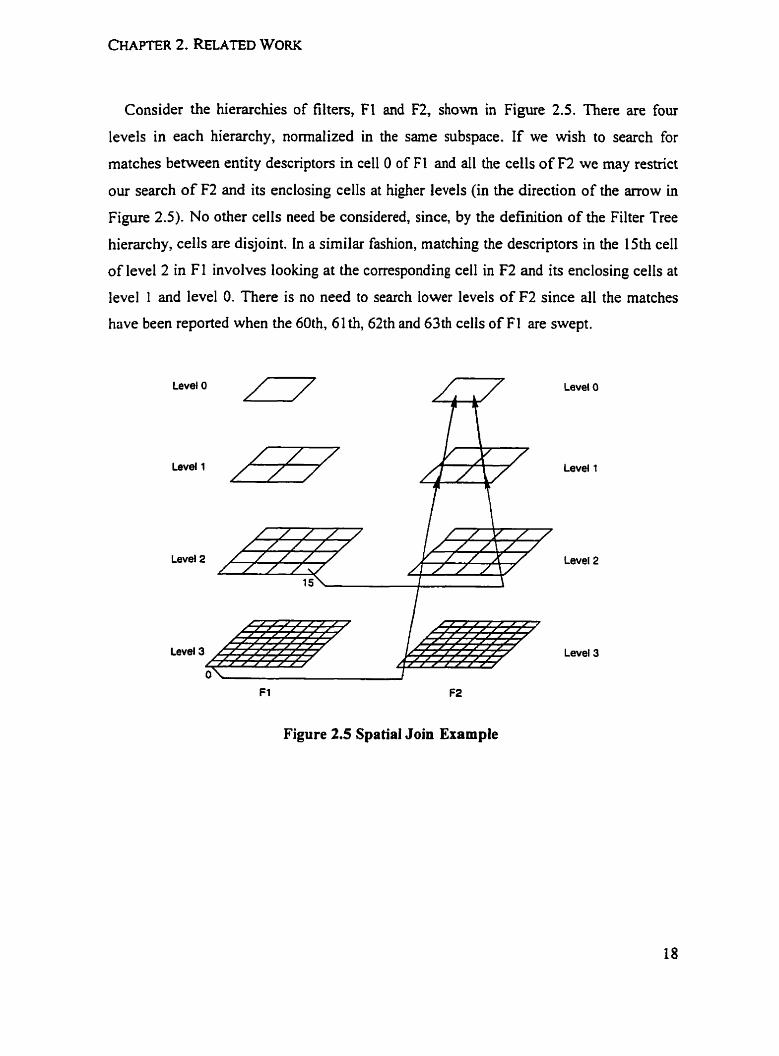
Consider the hierarchies of filters, FI and F2, show in Figure 2.5. There are four

levels in each hierarchy, normalized in the same subspace. If we wish to search for

matches between entity descripton in ce11 O of FI and al1 the cells of F2 we may restrict

our search o f F2 and its enclosing cells at higher levels (in the direction of the arrow in

Figure 2.5). No other cells need be considered, since, by the definition of the Filter Tree

hierarchy, cells are disjoint. in a similar fashion, matching the descriptors in the 15th ce11

of level 2 in F1 involves looking at the corresponding ce11 in F2 and its enclosing cells at

level 1 and level O. There is no need to search lower leveIs of F2 since al1 the matches

have been reported when the 60th, 6 1 th, 62th and 63th cells of FI are swept.

Level O Level O

Levd 1

Levei 3

Figure 2.5 Spatial Join Example

Chapter 3

Problem Statement

3.1 Motivation

Spatial data is more complicated to handle than one-dimensional data. Consider, for

example, in a GIS system, a series of line segments are used to represent roads. We may

ask "which road is closest to point p?" and "rank the roads by distance fiom point p." For

a fixed reference point p and distance meiric, a one-dimensional index on the distances of

the roads From point p will lead to an efficient execution time for this particular point.

However, it would be useless for any other points or distance meaics, and it is too

expensive to rebuild indices for every possible query point.

A more interesthg and at the sarne time more complex query would be to identifj the

closest object to a query point where additional conditions may be imposed on the object.

For exarnple, 'iank the roads by distance fiom city c for roads that have a speed limit less

than 80 km/hour." One rnethod is to sort al1 the roads by their distances fiom query point

c, and then apply the speed limit condition. This naïve solution turns out to be

impractical, since each time we need to re-sort the distance when we answer a similar

query with respect to another query point. A less radical solution is to retneve the closest

k road segments and detennine if any of them satisQ the speed lirnit critenon. However,

the problem here lies in detemiining the value of k. If k is too small, a failure in tuidhg

any road segments that fulfills the speed limit cntenon is very likely to happen. If k is too

large, a good portion of our work will be wasted since the speed limit of many roads will

never be checked.

A reasonable wap to overcome the disadvantages indicareci above is to obtam the

objects incrementally, as they are needed. To our knowledge, the existing incremental

solutions to the Distance Query al1 employ priority queues. However, the cost of priority

queue operations couid become significant in the incremental distance algorithms when

the size of the queue increases. In some cases, if the queue gets too large to fit in

memory, its contents must be stored in a disk-based structure instead of memory, making

each operation even more costly.

Another related question is, how should we store the road segments? Neither two-

dimensional points nor MBRs can represent al1 the important features of line segments.

The direction of the Iine is lost. And at the same time the accuracy is very important in

the distance-based quenes. For example, in a GIS system, MBRs are widely used to

approximate the real objects and it is very cornmon to have a 1 to 1,000,000 scale. In

other words, a deviation of 1 Millimeter in either the MBR approximation or the distance

calcuiation on the map corresponds to 1 Kilometer in real life. This means an error of 1

Millimeter in our calcuiation may dramatically change the results that are requested by

the usen who query a range with radius of 100 meters in real life.

We will mainly address the following two problems in our thesis:

1. What is the most efficient technique to perform distance-based queries on spatial

data? 1s there a way to overcome the drawbacks of a priority queue?

2. In dealing with line segments, what are the efficient approximations for the spatial

data to make distance-based queries mon accurate and more efficient?

3.2 Criteria for Eff~ciency

We have repeatedly mentioned the word efficiency in the problem statement. This may

refer to one of the two aspects of efficiency: space efficiency and time efficiency.

For space efficiency, the goal is to minimize the number of bytes occupied by the

index for the amount of information that is kept. For example, we may want to choose an

MBR to approximate a line segment. The MBR can e i h be specified by the coordinates

of al1 four corners or be specified by only the coordinates of the Iower left comer and the

upper right comer. Clearly, the latter representation of the MBR takes only half the space

of the former one. However, neither of the representations record the direction of the line.

So a representation that contains not only the Iower lefi and the upper right coordinates,

but also the sign of the slope, cannot be judged as less efficient though one extra bit is

required for each MBR index. For the sake of time efficiency and possible M e r

increase of the precision, we use an extra byte to store the slope in our implementation.

For time eficiency, the situation is not very clear. Elapsed time is obviously what the

user cares about. However, the corresponding measurements greatly depend on

irnplementation details, hardware utilization, and other external factors. So another

performance measure: the number of disk accesses performed during a search, seems to

be more objective in this context. This approach is based on the assumption that most

searches are VO-bound rather than CPU-bound, although this assumption is not always

tme. The great increases of the size of main memories make VO accesses less dominant,

but it is still an important goal to minimize that number of disk accesses. In our tests, we

examine not only the number of VOS but also the processor time and elapsed time in

response to each query.

3.3 Sphere Intersection Query and Distance Query

Distance-based queries refer to the queries that can only be answered by calculating the

distance between objects and comparing the distance with the query cntena. Comrnon

examples of distance-based quenes include Nearest-Neighbor Query and Distance Query,

which were formdly defined in Chapter 1. Here we discuss two specific distance-based

queries, Sphere Intersection Queries and Distance Quenes. Although these queries can be

answered using most spatial data structures, for concreteness we present these two

queries in the context of the Filter Tree. Also, performance tests are conducted on the

Filter Tree.

3.3.1 Spbere Intersection Queries

A Sphere Intersection Query can be regarded as a variation of the Range Query where the

query window is a circle or sphere rather than a rectangle. The circle is specified by a

query center and a radius. At the same time, a circumscribed square is determined. Like a

Range Query in the Filter Tree, at each containment level, the square will cover a certain

range of Hilbert values. Figure 3.1 shows us a query sphere where Level 3 is used as the

containment level. At level 3, Hilbert values 18 to 20, 22 to 25 and 29 are intersected by

the circumscnbed square.

Figure 3.1 Query Circle at Containment Level3

As in Range Quenes, a square is used as the query window to narrow d o m the range

of Hilbert Values that must be searched. Hence this square determines, at each level,

which data pages must be read. Once the data pages are read in, the distance between

each object of the page and the query center is calcuiated and compared with the radius.

M e r the cornparison of the distance, the objects that fulfill the distance criterion will

be copied to a page in the BufTer, when the page is ml, it is written to the output file. A

more thorough description of the Sphere Intersection query, as perforrned on the Filter

Tree, is given in Appendix A.

3.3.2 Dlstance Queries

The Distance Query is closely related to the Sphere Intersection Query in two-

dimensional Euclidean context. It can be divided into two steps. First, we perform a more

generalized Sphere Intersection Query. Here more generalized means that we have to

compare the distance with two values of the radius, the imer circle radius and the outer

circle radius. The result set will include the records having the distance between the imer

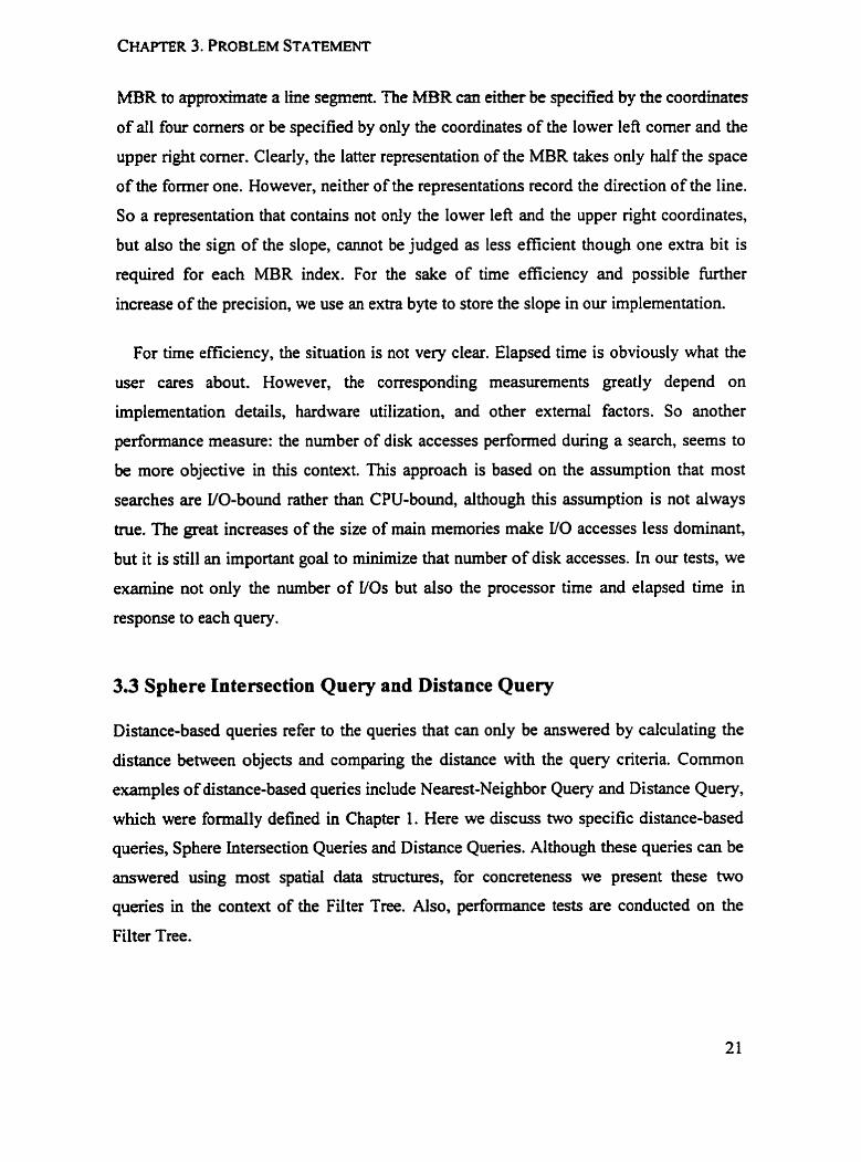
radius and the outer radius. Figure 3.2 illustrates the distances fiom the query point O to

points a, b and c, which are the centres of MBRs A, B and C. Only b satisfies the distance

criteria since only dist(0, Ob) E [Inner Radius, Outer Radius]. Second, instead of writing

ail the records that fùlfill the distance requirement back to the disk immediately, we need

to report the candidate records in an ascending order of distance frorn the query point.

As discussed in Chapter 3.1, the two naïve ways are not efficient in handling the

Distance Query, particularly if additional conditions are imposed on the object. Our

approach is that, right afler the distance to the query center is calculated, it is compared

with the query distance criteria. The top results are inserted into a sorted list, which

contains a fixed number of elements in the ascending order of distance. This incremental

algorithm will guarantee that effort in calculating the distance will not be wasted. The

structure of the Filter Tree makes this step very efficient:

We do not need to differentiate the leaf nodes and non-leaf nodes, which increases the

complexity of the distance calculation for other tree-like structures. Just recail that in

the Filter Tree, the entity descriptors are surteci according to the Hilbert value and

packed into contiguous blocks of secondary storage. Only entries that speciQ the

ranges of the Hilbert value are kept for each level of the tree. Each tirne, we simpiy

scan through the blocks that M l 1 the Hilbert value requirement. And this way. we

will guarantee that each block will be read in at most once.

We do not need to build the priority queue to store al1 the nodes that we have to

process as required by the incremental algorithm for other tree-like structures. For the

Filter Tree, again, we ody process the candidate entities within the Hilbert range.

While for R-Tree [Hjaltasûn and Samet 19991, for instance, al1 the leaf nodes that

have intersection with the query range need to be processed, and al1 the entities

contained in the leaf node need to be inserted into the priority queue. In some cases,

only a small portion of the entities in the pnority queue reside in the query range.

The pedormance of our incremental algorithm should be stable regardless of the size

of the datasets. However this is not dways true for other distance query algorithrns.

As we pointed out in Chapter 3.1, as the size of the dataset increases, it's very likely

that the queue size increases correspondingly, hence each operation becomes more

costly .

At the same time, new constraints on the query criteria can be easily enforced. For

example, when dealing with extraordinariiy large datasets, we can set an upper bound for

the number of rows that we have to process, or alternatively, an upper bound for the time

each query may take. Of course, these two constraints c m be applied at the sarne time in

order to guarantee that the query cm be accomplished in a reasonable time.

We will introduce two Distance Query algonthms for the centroid and slope datasets in

detail in Appendix B.

- - - - The border and slope of the MBR -.---.- The distance between the query center and the csntfoid d the MBR

Figure 3.2 Examples for Distance Query

A typicd Distance Query wiD need to retrieve oniy a very small fraction of the records

that are processed. For example, in a GIS application that contains 50,000 records of line

segments, it rnakes sense to ask 'Knd the nearest 20 roads fiorn city O within 5

kilometers". Because a general user will be very uniikely to ask for thousands of output

records, the user may be interested in the names of the roads with the shortest distance.

3.4 Accuracy in Distance Calculation

Accuracy formally means the degree of conformity of a measure to a standard or a true

value. Due to the discrepancy in the approximation of the spatial data and sometimes the

large scale between the reality and the model, a seemingly rninor error in the

approximation can be significant in real life.

This then leads to two sub-problems that need !O be addressed in the distance-based

query domain.

1. 1s there a more accurate approximation of the MBR that can minimize the

discrepancy for line segments?

2. Which distance function should be chosen to minimize the error?

3.4.1 Distance for MBRs without SIope

As mentioned in Chapter 3.1, the conventional representation for MBRs, by specimng

the lower lefi and upper right coordinates, loses the dope information. To answer the

distance-based queries, we choose to calculate the distance between the query center and

the centroid of the MBR. This distance is more appropriate than the d i s s c e beh~een the

query center and the nearest point of MBRs. This is true because it will have a greater

error when the line segment does not intersect the nearest corner of the MBR And for a

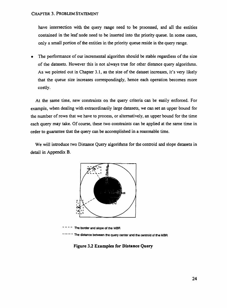
randomly distnbuted dataset, the chance for this mismatch is 50%. Figure 3.3 shows that

the distance nom query center O to line segment C. Suppose the line passes through the

lower right and upper left corners, the distance between O and the upper right corner

(XM) has the shortest distance, and it is smaller than the radius. However, the true

distance and the distance to Oc are greater than the radius, which causes an erroneous

response to the query. So it is safer and more consistent to use the distance between

centroid and the query center. Though this may also cause sorne mistakes, it is the best

we c m achieve without dope information.

-.-.---.- The border and the slope of îhe MER

The distance between ttie query center and the line segment

- - - - - The distance between the query center and the œntroid of the MBR . . . . . . . . . . The distance Mwwn the query center and the nearest point of the MBR

Figure 3.3 The Distance Between the Query Center and Centroid of the MBR Causes Big Discrepancy

It is reasonable to ask whether a set of line segments have to be stored as MBRs. This

question originates fiom the fact that, for a set of connected line segments, the upper right

coordinate of the previous segment is the lower left coordinate of the latter segment. It is

repetitive to store the same point twice. As an alternative, we can store the successive

corners of each line segment and no corner need be repeated. It is easy to observe that

this representation takes ody half the space that MBR takes up, however, it oniy works

with connected line segments while the MBR representation is more globally adaptive.

3.4.1 Distance for MBRs with Slope

Besides storing the coordinates for the MBRs, we propose another representation that

includes an integer to indicate the sign of the dope of the line segment associated with

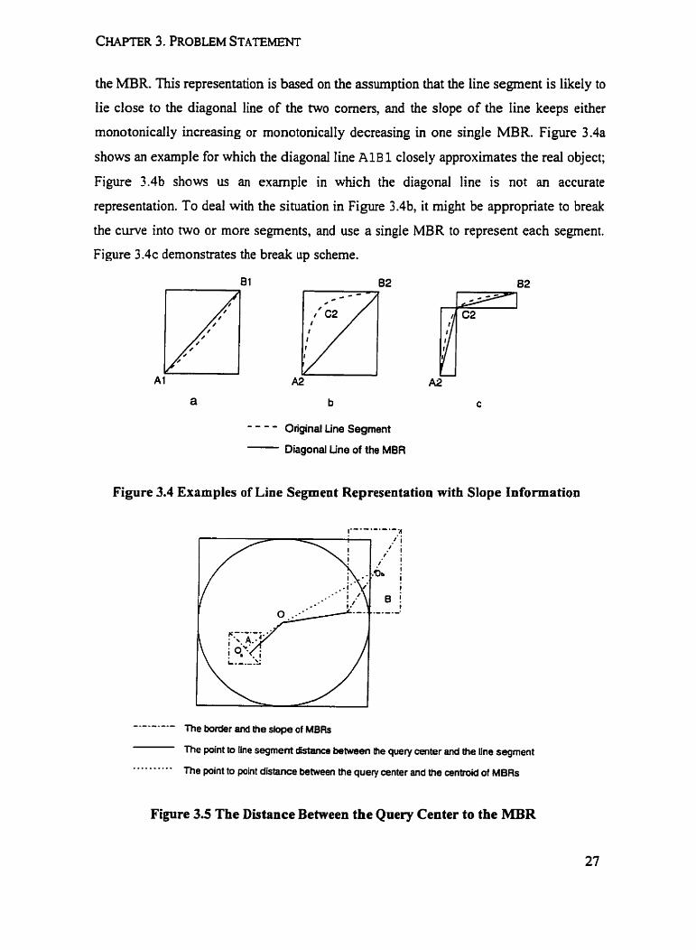
the MBR. This representation is based on the assumption that the line segment is likely to

lie close to the diagonal line of the two corners, and the dope of the line keeps either

monotonicaily increasing or monotonically decreasing in one single MBR. Figure 3.4a

shows an example for which the diagonal line A1B 1 closely approximates the real object;

Figure 3.4b shows us an example in which the diagonal line is not an accurate

representation. To deal with the situation in Figure 3.4b, it rnight be appropnate to break

the curve into two or more segments, and use a single MBR to represent each segment.

Figure 3 . 4 ~ demonstrates the break up scheme.

- - - - Original Line Segment - Diagonal Une of the MER

Figure 3.4 Examples of Line Segment Representation with Slope Information

1"-""-"A

-----*-.- The border and the dope of MBRs

The point to Iine segment distance between the query center and the line segment

. . * * . - - * * * The point to point distance between the query center and the œntroid of MBRs

Figure 3.5 The Distance Between the Qnery Center to the MBR

In this case, the distance is no longer simply between two points. Instead, as

demonstrated in Figure 3.5, the distance can be either to a corner or to the diagonal line

of the MBR. For example, the distance fiom O to object A is no longer the distance from

O to the centroid of object A; more precisely, it should be behveen O and dope of A. The

distance fiom O to object B is the distance between O and lower left corner of B.

Chapter 4

Experimental Setup

In order to test and compare the performance of the Sphere Intersection Query and the

Distance Query on the Filter Tree, we conducted a series of experiments using both

synthetic and real data sets. Al1 the expenments were performed on a Sun SPARCstation

5 machine with a total of 64MB memory ninning Sun Solaris 8 operating system.

4.1 The Questions and Anticipated Results

As mentioned in Section 3.3, we have demonstrated that the structure of the Filter Tree

makes the distance-based queries very efficient in theory. We are still interested in the

following questions.

1. Are the distance-based quenes sensitive to the size of the datasets?

2. What is the effect of the size and position of the query window on the response tirne?

3. Will the performance be stable when datasets are highly skewed?

4. For a distance query, how does the sorted Iist size affect the response time?

4.2 Synthetic Data Used

In order to test the performance of out dgorithms with different levels of skewed

datasets, we set up a set of synthetic data with a diagonal distribution in two-dimensional

space. Here diagonal distribution means that the centroids of the entities are distributed

dong the main diagonal. The levels of skew were used in a manner that the lower the

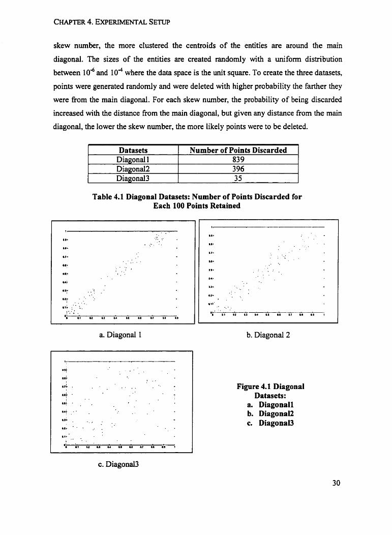
skew number, the more clustered the centroids of the entities are around the main

diagonal. The sizes of the entities are created randomly with a uniform distribution

between 1 o4 and 104 where the data space is the unit square. To create the three datasets,

points were generated randomly and were deleted with higher probabiiity the farther they

were fiom the main diagonal. For each skew number, the probability of being discarded

increased with the distance from the main diagonal, but given any distance from the main

diagonal, the lower the skew number, the more likely points were to be deleted.

I ~~~~~

Datasets 1 Number of Points Discarded ]

Table 4.1 Diagonal Datasets: Number of Points Discarded for Each 100 Points Retained

Diagonal 1 Diagonal2 Diagonal3

a. Diagonal 1

839 396 35

b. Diagonal 2

"t - . . 8It

I . -

a?! . . . . . . + . .

l l t - . . l 4 t ... . . .

Figure 4.1 Diagonal Datasets:

a. Diagonal1 b. Diagonai2 c. DiagonaW

Table 4.1 shows, for each of the three skews used, the number of points discarded to

generate a set of one hundred random points. The files of this set are referred to as

Diagonal 1, Diagonal2 and Diagonal3. These files were created with the following sizes:

10,000, 25,000, 50,000 and 100,000 because the sizes are similar to the sizes of the reaI

datasets used.

In Diagonall, with the highest skews, almost dl points are quite close to main

diagonal. in Diagonala, most of data space is occupied, but is denser around the main

diagonal. In Diagonal3, most of data space is occupied, and ody the upper-left comer

and lower-right comer are sparse. This is very close to a unifom distribution. The

distributions of three Diagonal sets are shown in Figure 4.1.

4.3 Real Data Used

The real data that is used in the experiments consists of five data sets, referred to as EC,

MA, OR, GT and CT respectively. Each dataset contains the longitudes and latitudes of

the objects, in our case, line segments.

EC represents the borders of countries on the European Continent. It consists of 25,959

rows, and each row describes a line segment. These line segments form 337 disjointed

regions,

MA and OR are denved fiom the T I G E m i n e File [Bureau of the Census 20001. MA

contains 66,908 line segments for Worcester, Massachusetts. OR contains 69.228 line

segments for Lane County, Oregon.

GT and CT are the geographicd data sets for Great Toronto Area and City of Toronto.

GT has 4,632 line segments and makes up 199 regions. Compared to GT, CT is much

more detailed, consisting of 96,844 line segments that make up 5370 regions in Toronto

City.

a. EC (Europe Map)

r 10'

b. MA (Worcester, MA)

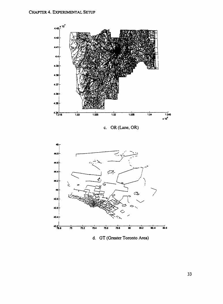
c. OR (Lane, OR)

a 2 78.0 79 79.2 7â4 79.6 7 â B 80 BQ2 811.4 846

d. GT (Greater Toronto Area)

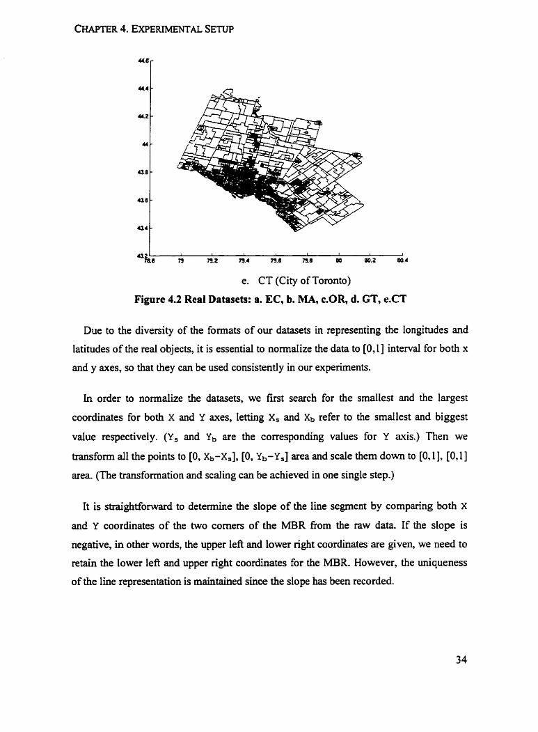
e. CT (City of Toronto)

Figure 4.2 Real Datasets: a. EC, b. MA, c.OR, d. GT, e.CT

Due to the diversity of the formats of our datasets in representing the longitudes and

latitudes of the red objects, it is essential to nomaiize the data to [OJ] interval for both x

and y axes, so that they can be used consistentiy in our experiments.

In order to normalize the datasets, we first search for the smallest and the Iargest

coordinates for both X and Y axes, lening X, and xb refer to the smallest and biggest

value respectively. (Y, and Yb are the corresponding values for Y a is . ) Then we

transform d i the points to [O, Xb-Xs], [O, Yb-Ys] area and scale them down to [O, 11, [0,1]

area (The transformation and scaling can be achieved in one single step.)

It is straightfonvard to determine the slope of the line segment by comparing both X

and Y coordinates of the two corners of the MBR fiom the raw data. If the slope is

negative, in other words, the upper lefi and lower right coordinates are given, we need to

retain the lower lefi and upper nght coordinates for the MBR However, the uniqueness

of the line representation is maintained since the dope has k e n recorded.

Thus, the sizes of the red datasets Vary fiom 4,632 rows to 96,844 rows. This enables

us to conduct our experiments on a wide range of sizes, therefore providing a sound basis

to examine the sensitivity of our aigorithms to the size of the datasets. Plots of the five

real datasets are shown in Figure 4.2.

We conducted our experiments on ail the five real datasets, and the results are

consistent. However, in order to make the presentation more concise, we randomly

choose only three result sets out of five to discuss in each experiment.

4.4 Query Windows Used

in order to test the effect of the size and position of the query window on the response

tirne, we set up nine query windows. Table 4.2 illustrates the coordinate of the query

center, the radius of the query and the fraction of the data space each query area covers.

--

Table 4.2 Query Windows

The first five query centers are located at the centroid of the data space with the radii

of 0.05, 0.10, 0.15, 0.20 and 0.25 respectively. The last four query centers reside at the

centroids of the four sub-squares of level 1 of the Filter Tree. Here we choose the radius

to be 0.15, which is the median value for the bt five query windows. Figure 4.3

illustrates al1 these nine windows,

Fraction of Data Space 0.79% 3.14% 7.07% 12.57% 19.93% 7.07% 7.07% 7.07% 7.07%

As we can see in Figure 4.3, the nine query windows have covered an essential part of

the data space. Ranging fiom 0.79% to 19.93% of the space, QI to Q5 are used to test the

Radius 0.05 0.20 O. 15 0.20 0.25 0.15 O. 15 0.15 0.15

Windows Qi 42 4 3 Q4 QS Q6 Q7 Q8 Q9

Center Coordinate (x, y) (0.5,0.5) (0.5,0.5) (0.5, 0.5) (0.5,OS) (0.5,0.5)

(0.25, 0.25) (0.25,0.75) (0.75,0.25) (0.75,0.75)

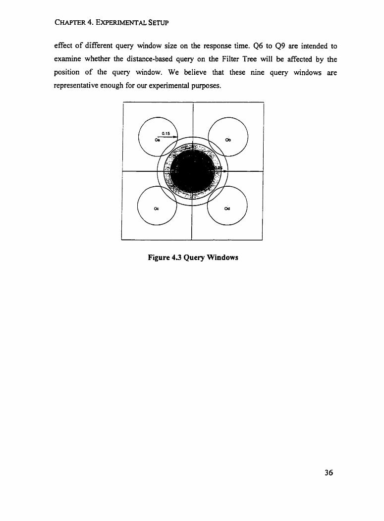
effect of different query window size on the response time. 46 to Q9 are intended to

examine whether the distance-based query on the Filter Tree will be affected by the

position of the query window. We believe that these nine query windows are

representative enough for our expenmental purposes.

Figure 4.3 Query Windows

Chapter 5

Experimental Results: Sphere Intersection Query

We conduct our experiments for Sphere intersection Query (SIQ) using two different

distance metrics: point to point (PTP) and point to line segment (PTLS) meûics. For

each of these wo distance metrics, we test our aigorithms on both synthetic datasets and

reai datasets. We record the nurnber of IlOs and the processor time, and compare the

costs for these two implementatiow. The purpose of these two experirnents is to:

1. Determine whether the performance of our aigorithms is stable over a range of test

conditions;

2. Detemine how the result sets of the two SIQ algorithms differ;

3. Determine whether the dope implementation is substantiaily more expensive than the

centroid one.

Experiments 1 and 2 test the SIQ Centroid and SIQ Slope algorithms respectively on

varying sizes of the synthetic datasets. Experiments 3 and 4 examine the effect of varying

the query window size on the response time. Experiments 5 and 6 test if the SIQ

algorithms are sensitive to the position of the query window.

5.1 Experiments 1 and 2: Varying the Size of the Dataset

In Experiments 1 and 2, our tests on the SIQ operation were conducted on the Diagonal

datasets. The sizes of the Datasets Vary h m 10,000 to 100,000. The medium sized query

window 43 is used.

CHAPTER 5. EXPERIMENTAL RESULTS: SPHERE INTERSECTION QUERY

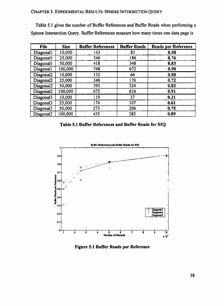
Tabh 5.1 gives the numbet of Buffer References and Buffer Reads when performing a

Sphere Intersection Query. Buffer References measure how many times one data page is

Size Buffer References Buffer Reads Reads per Reference 11 10,000 143 83 0.58 11 25.000 246 186 0.76

Table 5.1 Buffer References and Buffer Reads for SIQ

Figure 5.1 Buffer Reads per Reference

searched for some range of HiIbert vahes; BufEer Reads count the number of tirnes a

logical read is performed to read the pages into the buffer. Table 5.1 shows that both

BufTer References and Buffer Reads increase as the size of the datasets increases, the

B d e r Reads tend to increase at a faster rate than Buffer References. Figure 5.1 illustrates

this.

We observe that the above results are consistent with our expectation. The Filter Tree

we implemented makes use of a buffer of size 64 pages, where index pages are kept in

memory with higher prionty than data pages. Normally, the index pages will take

approximately half the buffer space and will reside there until the end of each operation.

The rest of the room in the buffer will be used to accommodate the data pages when they

are required in the Hilbert Value search. If the data page is still in the buffer when it is

requested again, this page is referenced more than once. However, the chance for one

page to be re-referenced tends to decrease when the dataset becomes very big, since that

page is more likely to have been replaced in memory by other data pages. This explains

why in our tests, only approximately 10% of the pages are referenced again when the

dataset contains 1 00,000 records.

File

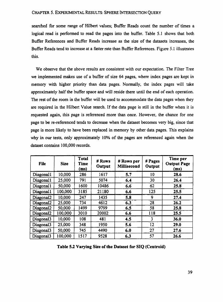
Table 5.2 Varying Size of the Dataset for SIQ (Centroid)

Diagonal1 Diagonal 1 Diagonal 1 Diagonal1

\

Size

10,000 25,000 50,000

. 1009000

Time (ms) 286 79 1 1600 3185

# ~ o w s Output

1

1617 5074 10486

, 21180

# ~ o w s per Millisecond

5.7 6.4 6.6

# Pages Output

Time per OUtPUt

(ms)

6.6 t 125 1 25.5

10 30 62

28.6 26.4 25.8

CHAPTER 5. EXPEIUMENTAL RESULTS: SPHERE INTERSECTION QUERY

t

File

Diagonal 1

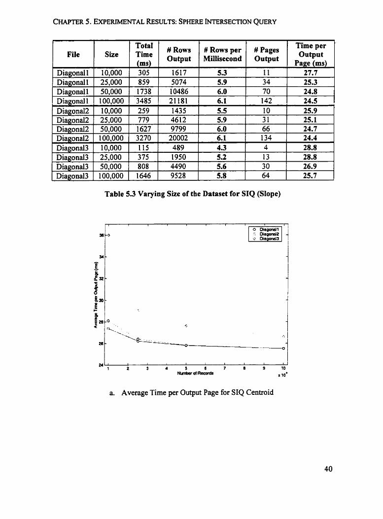
Table 5.3 Varying Size of the Dataset for SIQ (SIope)

- -

Diagonal 1 Diaeonall

a. Average Time per Output Page for SIQ Centroid

25,000 50.000

' # ~ o w s per Mihecond

5.3

' # ~ o w s Output

1617

L

10,000

'

Tim; rns 305 859 1 738

' # Pages Output

11

per '

Output

27.7 5074 1 0486

5.9 6.0

34 70

25.3 24.8

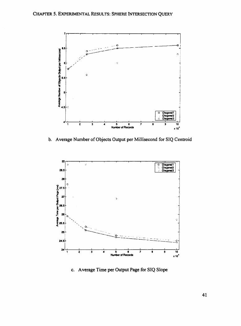
b. Average Number of Objects Output per Millisecond for SIQ Centroid

c. Average Time per Output Page for SIQ Slope


&2, 8 I I

d. Average Number of Objects Output per Millisecond for SIQ Slope

Figure 5.2 Varying the Size of the Datasets

Figure 5.2 is denved fiom Table 5.2 and Table 5.3, it shows the effects of varying size

of the datasets on SIQ operation. Figure 5.2a and Figure 5 . 2 ~ demonstrate that for both

centroid and dope implementation, as the size of the input file increases, the average time

spent on each output page tends to decrease. Accordingly, Figure 5.2b and Figure 5.2d

show that the average number of rows produced per millisecond increases.

We observe that the TotaI Time (TT) can be divided into two parts, namely Overhead

Time (OHT) and Output Time (O PT). We defme the following formula:

TT = OHT + OPT;

The above formula c m also be expressed in the following form:

TT = OHT + AOPT * NOP;

where AOPT denotes Average Output Time per page and NOP denotes Number of Output

Pages. We expect that the OHT and AOPT to be nearly constant for each query range if

the NO P is in a reasonable range. Here reasonable means no less than three pages, since if

the result set contains only one or two pages, and if the page contains only a smdl portion

of the potentid capacity of a data page, thm the average t h e per page becornes

meaningless.

a. AOPT vs. OHT for SIQ Centroid

b. AOPT vs. OHT for SIQ Siope

Figure 5.3 Average Output Time and Overhead Time for SIQ

Based on the resdts we obfained fiom TabIe 5.2 and Tabie 5.3, we derive two Iinear

fits that interpolate the AOHT and OHT for Diagonal1 dataset. As shown in Figure 5.3a

and Figure 5.3b, the AOPT and OHT are ahos t constant. This helps to explain why the

average time per output page will decrease in Figure 5.2a and Figure 5 .2~ : suppose that

OHT is a constant, so the larger the number of output pages, the srnailer that page's share

of the overhead is. However, this effect becomes weaker and weaker as the number of

output pages grows. That's why in Figure 5.2a and Figure 5 . 2 ~ the decreasing rate in

average time per output page slows down as the output size increases. This property will

make our estimation for the execution time more precise.

File

Diagonal 1

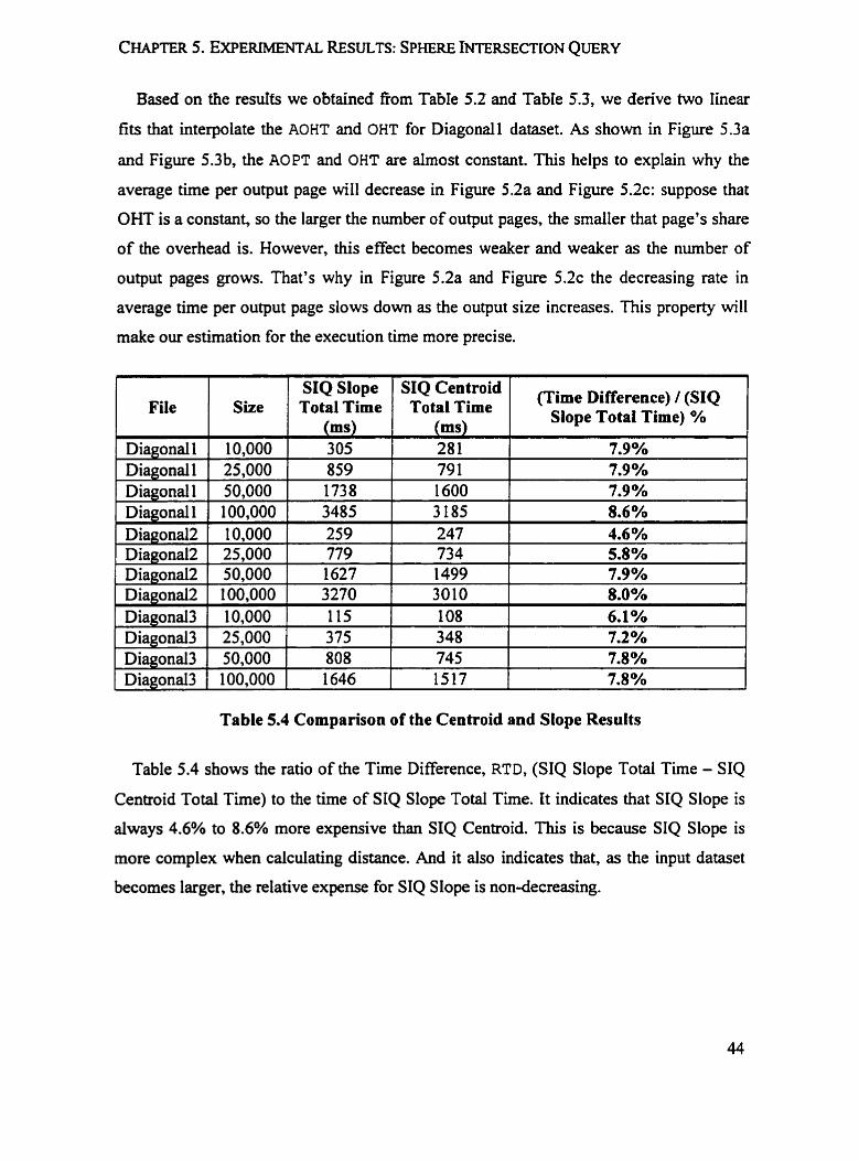
Table 5.4 Cornparison of the Centroid and Slope Results

Diagonal 1 Diagonal 1

Table 5.4 shows the ratio of the Tirne Difference, RTD, (SIQ Slope Total Time - SIQ

Centroid Total Time) to the time of SIQ Slope Total Tirne. It indicates that SIQ Slope is

always 4.6% to 8.6% more expensive than SIQ Centroid. This is because SIQ Slope is

more complex when calculating distance. And it also indicates that, as the input dataset

becomes larger, the relative expense for S IQ S lope is non-decreasing.

Size

10,000 25,000 50,000

SIQ Slope Total Time

(ms) 305 859 1738

SIQ Centroid Total Time

(ms) 28 1

(Time Difference) / (SIQ Slope Total Time) %

7.9% 79 1 1600

7.9% 7.9%

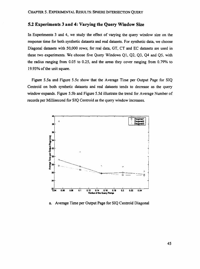
53 Experiments 3 and 4: Varying fhe Query Window Size

In Experiments 3 and 4, we study the effect of varying the query window size on the

response time for both synthetic datasets and real datasets. For synthetic data, we choose

Diagonal datasets with 50,000 rows; for real data, GT, CT and EC datasets are used in

these two experiments. We choose five Query Windows QI, Q2, 43, 44 and Qj, with

the radius ranging from 0.05 to 0.25, and the areas they cover ranging from 0.79% to

19.93% of the unit square.

Figure 5.5a and Figure 5 . 5 ~ show that the Average Time per Output Page for SIQ

Centmid on both synthetic datasets and real datasets tends to decrease as the query

window expands. Figure 5.5b and Figure 5.5d illustrate the trend for Average Nurnber of

records per Millisecond for SIQ Centroid as the query window increases.

a. Average Time per Output Page for SIQ Centroid Diagonal

b. Average Number of Objects Output per Millisecond for SIQ Centroid Diagonal

24l I 1 I 1 1 I 1 1 I

0û4 Qû6 Qûû 01 a12 al4 016 h l 8 02 O . QU Radus of * Quay Ra-

c. Average Tirne per Output Page for SIQ Centroid (Real Datasets)


/----- ---]

---- - /----- --y --

o s 1 1

i I

I i

I 1

< I

1 - 1 O

EC O - 1 1 1 1 1 I

401 0.06 A M û.1 0.12 0.14 0.16 0 . 8 û.2 0.22 0.24 Radw of Ihe Qucry Range

d. Average Number of Objects Output per Millisecond for SIQ Centroid (Real Datasets)

Figure 5.5 Varying the Query Window Sue for SIQ Centroid

a Average Time per Output Page for SIQ Slope (Diagonal)

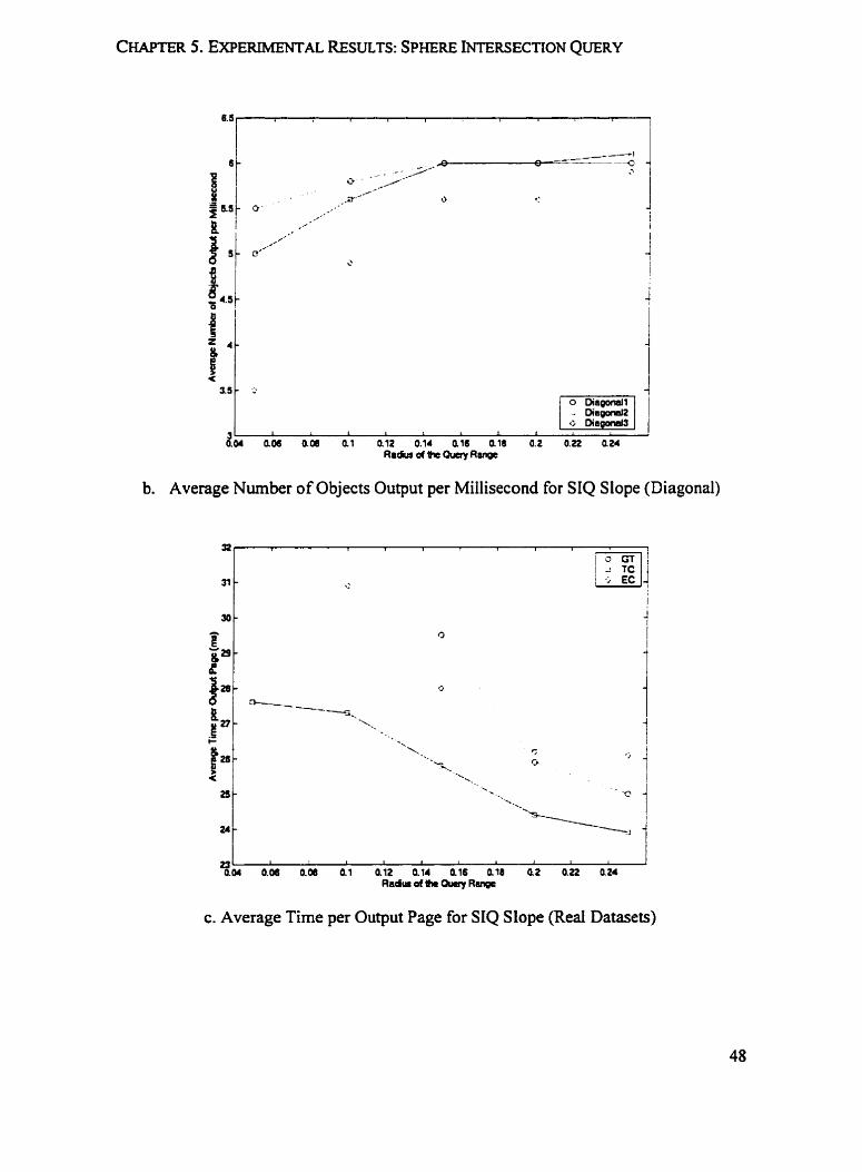
b. Average Number of Objects Output per Millisecond for SIQ Slope (Diagonal)

c. Average T h e per Output Page for SIQ Slope (Real Datasets)

3 ' "' O 1 I I 1 * atn 0.06 o . a i 0.12 0.94 ai6 0.18 0.2 0.a a24

Radw d Ihc Gucry Ronge

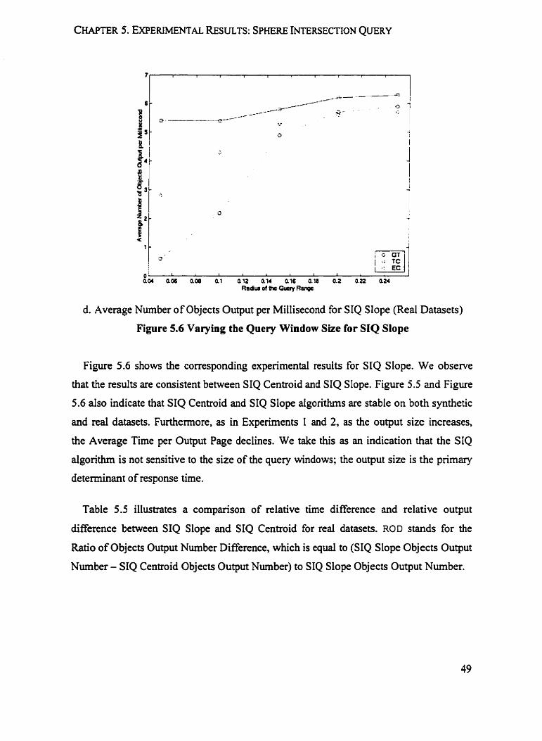
d. Average Number of Objects Output per Millisecond for SIQ Slope (Real Datasets)

Figure 5.6 Varying the Query Window Size for SIQ Slope

Figure 5.6 shows the corresponding expenmental resdts for SIQ Slope. We observe

that the resuits are consistent between SIQ Centroid and SIQ Slope. Figure 5.5 and Figure

5.6 aiso indicate that SIQ Centroid and SIQ Slope aigonthms are stable on both synthetic

and red datasets. Furthermore, as in Experiments 1 and 2, as the output size increases,

the Average Time per Output Page declines. We take this as an indication that the SIQ

algorithm is not sensitive to the size of the query windows; the output size is the primary

determinant of response time.

Table 5.5 illustrates a cornparison of relative t h e difference and relative output

ciifference between SIQ Slope and SIQ Centroid for real datasets. ROD stands for the

Ratio of Objects Output Number Difference, which is equal to (SIQ Slope Objects Output

Number - SIQ Centroid Objects Output Number) to SIQ Slope Objects Output Number.

Table 5.5 Time Difference and Output Difference between SIQ Slope and SIQ Centroid for Varying Size of Query of Query Window

Consistent with our results shown in Table 5.4, the percentage of RTD varies between

L

C

GT GT GT GT GT CT

4.3% and 8.6%. Except for one extreme case, ROD is substantially smaller compared to

' (Time Difference) I @QS Total Time) %

43% 5.4% 8.1% 6.6% 6.9% 8.0%

Query Window

Ql 42 43 44 Qs QI

RTD. This is because the real data we used is very detailed. In other words, the difference

' ROD

14.3% 0.8% 0.6% 0.1% 0.1% 0.7%

between the two distance metrics is not very remarkable for these datasets.

One more observation regarding the output nurnber difference is that, the number of

records produced by the Slope implementation is never less than that of the Centroid

implementation. Recall that, when we know the slope, we measure to the closest point on

the inferred diagonal line. That distance is guaranteed to be less than or equal to the

distance to the centroid, with equality occurring only if the inferred line happens to be

perpendicular to the line fiom the query point to the centroid.

5.3 Experiments 5 and 6: Varying the Query Window Position

The purpose of these two experiments is to check the effect of varying the query window

position on the response tirne. For synthetic datasets, we stiU make use of Diagonal

Datasets with 50,000 line segments; for real datasets, we choose MA, OR and EC. Four

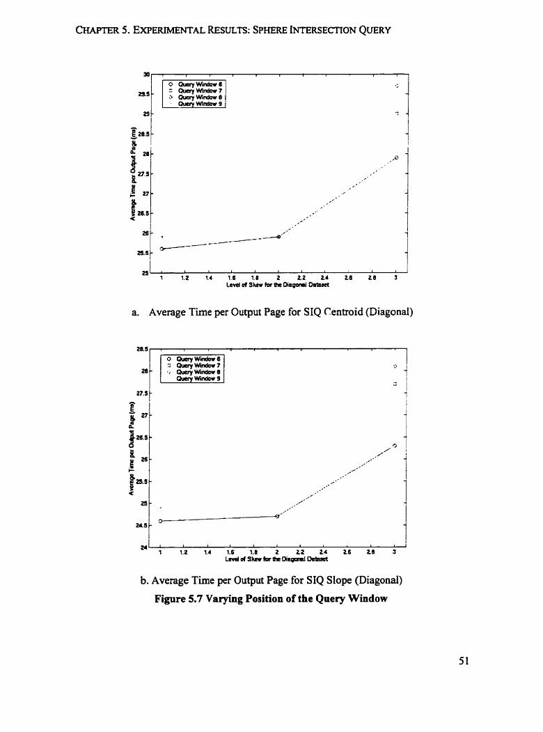
a. Average T h e per Output Page for SIQ Centroid (Diagonal)

b. Average T h e per Output Page for SIQ Slope (Diagonal)

Figure 5.7 Vsrying Position of the Query Window

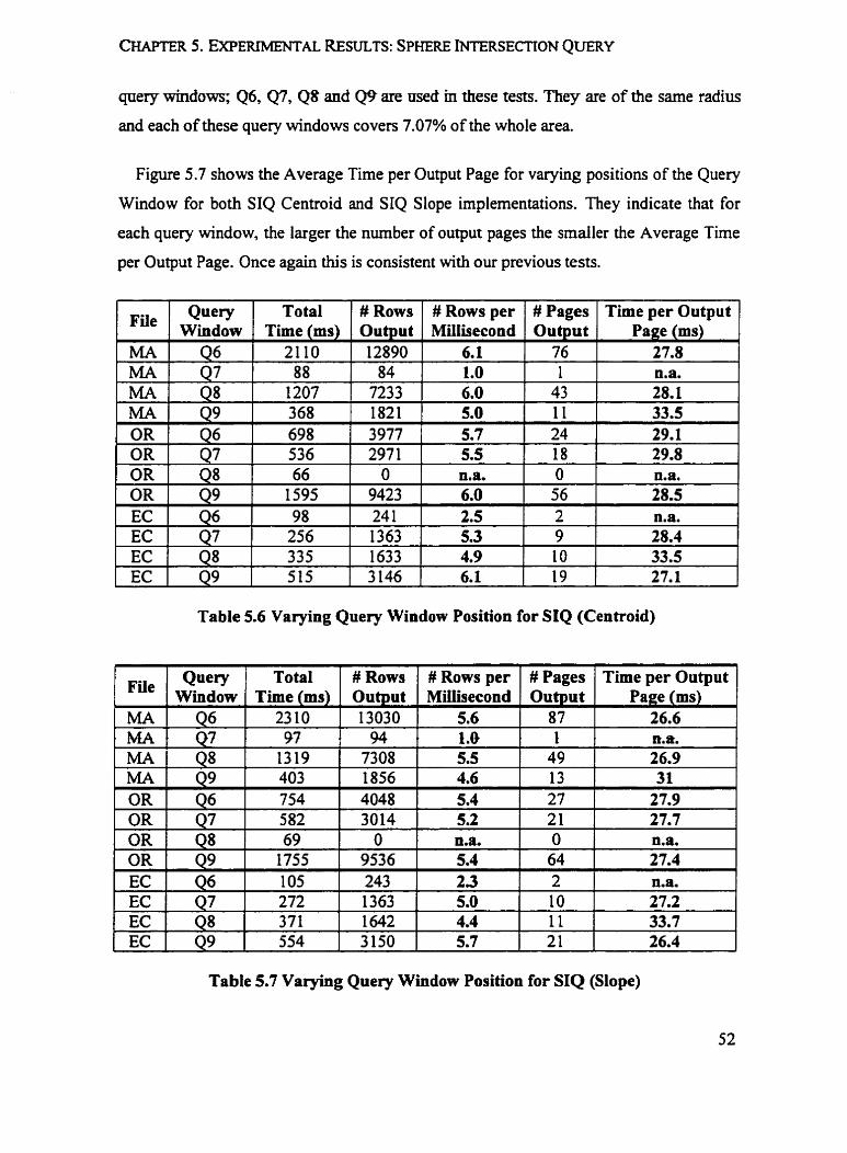
q n q windows; 46, 47, Q% and Q9 are wed in these tests. They are of the same radius

and each of these query windows coven 7.07% of the whole area.

Figure 5.7 shows the Average Time per Output Page for varying positions of the Query

Window for both SIQ Centroid and SIQ Slope implementations. They indicate that for

each query window, the larger the nurnber of output pages the srnaller the Average Time

per Output Page. Once again this is consistent with our previous tests.

Table 5.6 Varying Query Window Position for SIQ (Centroid)

Q u e r ~

Table 5.7 Varying Query Window Position for SIQ (Slope)

File Window Time (ms) Output Millisecond Output Page (ms) I

Total

,

MA

# Rows

Q u e r ~ Window

0 6

# Rows per

Total Time (ms)

2310

# Pages

# Rows Output 13030

Time per Output

# Rows per Millisecond

5.6

# Pages Output

87

Time per Output Page (ms)

26.6


One more observation on Figure 5.7 is that, by symmetry, we wouId expect the Iines

for 46 and Q9,Q7 and Q8 to be identicai respectively, however due to the randomness of

the synthetic datasets, there is a small discrepancy between the corresponding results.

Since 47 and Q8 are placed at the sparse corners of the data space, the Nurnber of Output

(HOP) does not fa11 in a reasonable range for Diagonal 1 and Diagonal 2, so for 47 and

Q8, only the data for Diagonal 3 is available.

Similar conciusions can be drawn fiom Table 5.6 and Table 5.7, which contains results

based on real datasets.

5.4 Experiments Summary

We have the following conclusions fiom the expenments that we conducted.

1. The SIQ algonthms on the Filter Tree preserve a stable performance regardless of the

Input Data Size, the Query Window Size and the Query Position.

0 With a suficient nurnber of output pages (>3) , the size of the output seems to be

the primary determinant of the response time. We can rather precisely estimate

the response time if we know the output size.

The SIQ Centroid and SIQ Slope implementations share similar behavior on both

synthetic and real datasets.

2. The SIQ Slope is always 4% to 9% more expensive than SIQ Centroid in the term of

time eficiency. Whife due to the tiigh quatity of the r d data, the relative output

difference (ROD) is only approximately 1%. Note that the number of objects in the

result set is usually on the order of thousand. This makes a difference when the

accuracy of the query is assessed.

Chapter 6

Experimental Results: Distance Query

The Distance Query (DQ) algorithm we proposed on the Filter Tree employs sorted list to

store the output in order of ascending distance. The algorithm can be divided into two

steps:

1. Fil1 up the output list without sorting it. We quick-sort the list for the first time either

when the list is full or the total number of output records is smaller than the list size.

M e r sorting, the algorithm will terminate if the latter case is tme; othenvise the

distance of the last record will be set up as the distance critenon.

2. If the candidate record has smaller distance than the distance criterion, it will replace

the last element in the list, and then a bubbIe sort &er the replacement will put the

list in order again by simply moving the last element upward to its appropriate

position in the list.

Similar to our experiments in Section 5, we conduct our tests for Distance Query on

PTP and PTLS rnetrics using both synthetic and real data. The number of VOS, the

number of records processed, the number of sorts and the processor time are recorded ta

evaiuate the performance of the two implementations.

Experiments I and 2 examine the DQ Centroid and DQ Slope algorithms on varying

sizes of the synthetic data. Experiments 3 and 4 test the effect of varying the query

window size on the response time. Besides testing stability and t h e efficiency of the DQ

algorithms, Experiment 5 and 6 are designed especially to examine the efYect of vax-ying

the sorted list size to the response time.

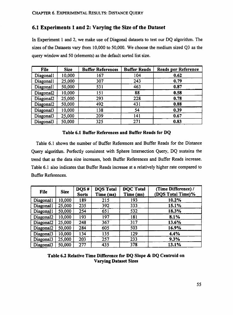
6.r Experiments f and 2: Varying the Size of the Dataset

In Experirnent 1 and 2, we make use of Diagonal datasets to test our DQ algorithm. The

sizes of the Datasets Vary fiom 10,000 to 50,000. We choose the medium sized 43 as the

query window and 50 (elements) as the default sorted list size.

Table 6.1 Buf'fer References and Buffer Reads for DQ

Table 6.1 shows the nurnber of Buffer References and Buffer Reads for the Distance

File Diagonal 1 Diagonal1 Diagonal1 Diagonal2 Diagonal2 Diagonal2

Query algorithm. Perfectly consistent with Sphere Intersection Query, DQ sustains the

Size 10,000 25,000 50,000 10,000 25,000 50.000

Buffer References 167 307 53 1 151 293 492

trend that as the data size increases, both B a e r References and Buffet. Reads increase.

Table 6.1 also indicates that Buffer Reads increase at a relatively higher rate compared to

Buffer Reads 1 04 243 463 88

228 43 1

Buffer References.

Reads per Reference 0.62 O. 79 0.87 rn

0.58 0.78 0.88

Table 6.2 Relative Time DEference for DQ SIope & DQ Centroid on Varying Dataset Sizes

(Time Difference) / @QS Total Tirne)%

10.2% 15.1% 18.3% 8.1% 13.6% 16.9% 4.4% 9.3 YO 13.1%

File

Diagonal1 Diagonal 1 Diagonal1 Diagonal2 Diagonal2 Diagonal2 Diagonal3 Diagonal3 Diagonal3

10,000 25,000 50,000 10,000 25,000 50,000 10,000 25,000 50,000

DQC Total Time(ms)

193 333

DQS # Sorts

, 189 235

DQS Total Time(ms)

215 392

254 193 248 284 134 203 277

65 1 1 532 197 367 605 135 257 435

181 317 503 129 233 378

Table 6.2 shows that as dataset size hcreases, the Number of Sorts, the TotaI Response

Time for both DQ Slope and DQ Centroid keep increasing. Furthemore, as illustrated in

Figure 6.2, the Relative Time Difference (RTD) grows for the increasing size of data.

Figure 6.1 Relative Time Difference between DQ Slope and DQ Centroid on Varying Dataset Sizes

We observe that the Total Time (TT) can be divided into three parts, namely Overhead

time (OHT), Distance Calculating Time ( K T ) and List Sorting Time (LST).

TT = OHT + DCT + LST;

We expect OHT to be a constant for eech qwry range; DCT linearly depends on the

number of rows being processed; LST depends on the nurnber of sorts in each query. In

other words, the above formula can be expressed in the following format:

TT = OHT + DCTPR * NRP + LST;

where DCTPR denotes Distance Calculating Time per Record and NRP denotes Number

of Rows Processed.

Since the OHT should be identical for the same query range and the nurnber of sorts is

very similar between DQ Slope and DQ Centroid on Diagonal datasets, we expect the

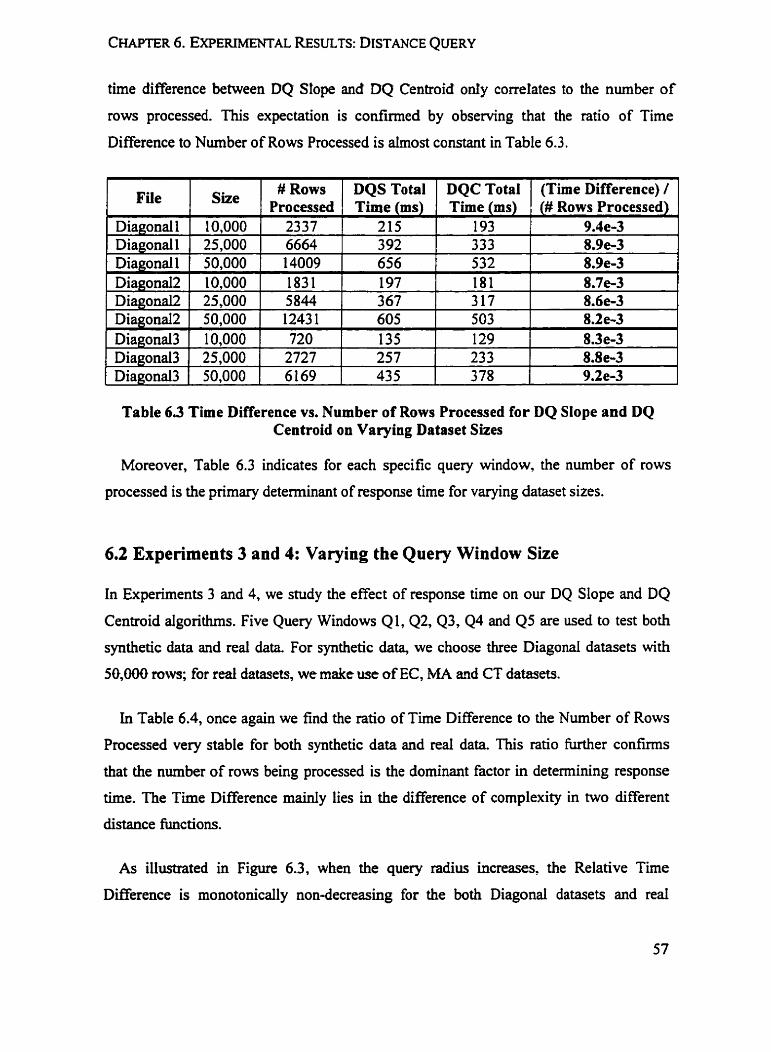
t h e difference between DQ Slope and DQ Centroid ody corretates to the number of

rows processed. This expectation is confmed by observing that the ratio of Time

Difference to Number of Rows Processed is ahos t constant in Table 6.3.

# Rows 1 DQS Total 1 DQC Total 1 1 size 1 Pmeesred Time Imsl Time Imsl

Table 6.3 Time Difference vs. Number of Rows Processed for DQ Slope and DQ Centroid on Varying Dataset Sizes

(Time Difference) / Mt Rows Proceosid)

Diagonal 1 Diagonail

Moreover, Table 6.3 indicates for each specific query window, the number of rows

processed is the primary detenninant of response time for varying dataset sizes.

10,000 25,000

6.2 Experiments 3 and 4: Varying the Query Window Size

Diagonal1 1 50,000

in Experirnents 3 and 4, we study the effect of response time on our DQ Slope and DQ

Centroid algorithrns. Five Query Windows Ql,Q2, 43, 44 and Q5 are used to test both

synthetic data and real data. For synthetic data, we choose three Diagonal datasets with

50,000 rows; for d datasets, we make use of EC, MA ami CT datasets.

2337 6664

In Table 6.4, once again we find the ratio of T h e Difference to the Nurnber of Rows

Processed very stable for both synthetic data and real data. This ratio further confirms

that the number of rows being processed is the dominant factor in determining response

time. The T h e Difference maidy lies in the difference of complexity in two different

distance functions.

14009

As illustratted in Figure 6.3, when the query radius increasesl the Relative T h e

Difference is monotonically non-decreasing for the both Diagonal datasets and reai

215 392 656

193 333

9.4e-3 8.9e-3

532 8.9e-3

datasets. And for synthetic data, the RTD c m take up to 19.4% of the DQ SIope Response

Time, th is ratio is as hi& as 20.7% of the DQ Slope Response Time for real datasets.

Figure 63a. Relative Time Difference between DQ Slope and DQ Centroid for Varying Query Window Sues (Synthetic Data)

Figure 63b. Relative Time Difference between DQ Slope and DQ Centroid for Varying Query Window Sizes (Real Dataseta)

CHAPTER 6. EXPER~MENTAL RESULTS: DISTANCE QUERY

Table 6.4a. Time Difference vs. Number of Rows Processed for DQ Slope and DQ Centroid (Synthetic Datasets)

Fiie

Diagonal 1 D i a g o n a l l A

Table 6.4b. Time Difference vs. Number of Rows Processed for DQ Slope and DQ Centroid (Real Datasets)

Diagonal 1 43 14009 656 532 8.9e-3 Diagonal 1 04 1853 1 848 688 8.6e-3

Query Window Ql

, EC EC EC EC EC MA MA MA MA MA

It is interesthg to observe that the increasing speed of RTD is getting slower when 43

and bigger query windows are used. This is largely due to the increase of the denominator

# Rows Processed 3295 8062

Query Window Ql 4 2 43 44 QS Ql Q2 Q3 Q4 0 5

# Rows Processed

317

' DQS Total Time (ms)

279 494

' DQC Total T h e (ms)

249 424

' (Time DitTerence) I (# R o m Processed)

9.le-3 8.7e-3

DQS Total Time (ms)

105

'

DQC Total Time (ms)

1 03 1094 3 863 6368 10608 1605 5319 12813 20858 31950

(Time Difference) / (# Rows Processed)

63e-3 158 266 356 484 161 329 533 936 1280

167 297 412 575 175 376 63 5 1119 1536

8.2e-3 8.0e-3 8.8~-3 8.6e-3 8.7e-3 8.8e-3 8.Oe-3 %.Se-3 -,

8.0e-3

(Srope Totai Thne). That is why even tEiough the T h e Difference is increasing the effect

of RT D findiy reaches a plateau.

6.3 Experiments 5 and 6: Varying the Size of Sorted List

The purpose of Experiments 5 and 6 is to check the effect of varying sizes of sorted list

on the Distance Query response time. For synthetic data, we use the Diagonal datasets

with 50,000 line segments; for real data, we choose EC, MA and CT. Four sorted lists,

with sizes 1 0,25, 50 and 1 00 respective1 y, are set up in these two tests.

- - --

Table 6.5a. Varying Sorted List Size for DQ Slope & DQ Centroid (Synthetic Data)

File

DQC Total Time (ms)

43 1 466 532 790 398 433 503 788 265 300 378 610

Diagona Diagona Diagona Diagona Diagona Diagona Diagona

.

Diagonal 1 Diagonal 1 Diagonal 1 Diagonal1 Diagonal2 D iagonal2 Diagonal2 Diagonal2 Diagonal3 Diagonal3 Diagonal3 Diagonal3

~ i a ~ o n a Diagona Diagona Diagona Diagona

DQS # Sorts

77 156 254 453 66 148 284 479 86 173 277 429

Sorted ~ i s t ~ i z e

10 25 50

. 1 O0 i0 25 50 1 O0 10 25 50 1 O0

Sorted # Rows Time (Tirne Difference) / @QS 1 List Size 1 Proeesed 1 DifTerenre

Table 6.5b. Varying Sorted List Size for DQ Slope & DQ Centroid (Synthetic Data)

DQC Y Sorts

77 156 253 453 66 148 284 482 86 173 277 428

DQS Total Tirne (ms

555 588 656 909 506 540 605 895 319 355 435 662

We observe in Table 6.5, as the sorted Iist sue increases, the TotaI Response Time wiII

increase for both DQ Slope and DQ Centroid. This is consistent with our intuitive

expectation because keeping a larger list in order involves more sorts of the list. At the

same tirne, the cost for each sort is generally more expensive for a larger list. This

expectation is also confumed by our experimental results.

Furthemore, we notice fiom Table 6.5b that the T h e Difference between DQ Slope

and DQ Centroid within each dataset is almost constant. Again this is consistent with our

intuition that the tirne difference between DQS and DQC for varying sorted list size is

primarily the time difference in distance calculation beh~een the PTP and PTLS distance

metrics. Because the Number of Rows Processed for each dataset is constant and the

Number of Sorts Difference between DQ Slope and DQ Centroid for Diagonal datasets is

very srnall, the effect of Number of Sorts in the Time Difference cm be ignored. Figure

6.4a illustrates the Time Difference between DQS and DQC for Varying Sorted List Size.

And Figure 6.4b shows the decreasing trends of RTD as the sorted list size increases.

Figure 63s. Time Dinerence between DQ Slope and DQ Centroid for Varying Sorted List Size (Centroid Data)

Sim of SorW Lisî

Figure 63b. Relative Time Difference behveen DQ Slope and DQ Centroid for Varying Sorted List Size (Synthetic Data)

DQS Total DQC Total DQS # SO* DQC # sorts Tirne (mr ~ i s t ~ ù e Time (ms)

-- - -- -

Table 6 . 6 ~ . Varying Sorted List Size for DQ Slope and DQ Centroid (Real Data)

Table 6.6b. Varying Sorted List Size for DQ Slope and DQ Centroid (Real Data)

C

EC EC EC EC

Table 6.6 shows the DQ Slope and DQ Centroid results for varying size of sorted list

on real datasets. We cm see that the Number of Sorts, the Total Response Time, Time

Difference and RTD al1 keep the similar trends as Diagonal dataset. However, the Time

Difference for MA and CT datasets is not perfectly stable. We observe that the Number

of Sorts Difference between DQS and DQC for these two datasets is no Ionger small

enough to be ignored. In other words, the Time Difference in sorting the list makes some

contribution to the Total Time Difference. If we take this factor into consideration, we

can still draw the conclusion that the time difference between DQ Slope and DQ Centroid

is almost constant.

Figure 6.4a illustrates the Tirne Difference between DQS and DQC for real datasets for

Varying Sorted List Size, and Figure 6.4b shows the decreasing trends of RTD as the

sorted list size increases.

' Sorfed List Size 10 25 50 1 O0

' Time Difference

34 32 31 33

' #Rows Proeessed

3863 3863 3863 3863

b

(Tirne Difference) / @QS Total Time) %

15.8% 13.1% 10.4% 6.8%

Figure 6.4a. Time Difference between DQ Slope and DQ Centroid for Varying Sorted List Size (Real Datasets)

0 L O 10 20 30 40 50 W 70 ûû 90 I W 110

Size of Sorted List

Figure 6.4b. Relative Time Difference between DQ Slope and DQ Centroid for Varying Sorted List Size (Real Datasets)

CHAPTER 6. EXPER~MENTAL RESULTS: DISTANCE QUERY

6.4 Experiments Summary

We can àraw the following conclusions fiom the experimental results above:

1. The DQ algorithms have a stable performance regardless of the Input Data Size, the

Query Window Size and Sorted List Size.

DQ Slope and DQ Centroid have similar behavior on Response Time, Number of

VOS and Number of Sorts on both synthetic data and real data.

The Response Time can be precisely predicted d e r knowing the size of the

Query Window, the Number of Records to be pmcessed and the size of output

list; and these three factors are the primary determinant of Response Time.

2. The Relative Time Difference (RTD) between DQ Slope and DQ Centroid can be as

hi& as 24.2% of the Total Response Time. For both synthetic data and real data, the

tirne difference is mainly caused by the different distance functions.

Chapter 7

Conclusions and Future Work

7.1 Conclusions

In this thesis, we have presented two algorithms to answer two distance-based quenes,

namely the Sphere Intersection Query (SIQ) and the Distance Query (DQ). Both of these

two algorithms make use of the Filter Tree as the spatial index. Experiments were

perfonned on both centroid datasets and slope datasets.

For both Sphere Intersection Query and Distance Query, the experimental results show

that the total response time can be precisely estirnated. For SIQ, the primary response

time determinant is the output size; for DQ, the total response tirne is primarily

determined by the number of records that we have to process, the size of the output list

and the choice of the distance function. We observe that stable performance is achieved

maidy due to the structure of the Filter Tree. Unlike dl the other DQ algorithrns. our

algorithm is straighdorward. There is no need to diflerentiate the leaf nodes and the non-

leaf nodes in the Filter Tree as in other tree structures. We simply scan through the files

that contain the candidate cells within the possible Hilbert value range.

The Total Response T h e for the Slope datasets is always 3% to 24.2% longer than the

corresponding Centroid datasets for both SIQ and DQ. The percentage of difference

keeps increasing as the number of output records increases. This difference is mainly

because of the difference in complexity in caiculating distance using slope and centroid

datasets.

7.2 Future Work

7.2.1 Data with Higher Dimensionality

In the implementation of SIQ and DQ algorithms, we need to calculate the Hilbert values

in two-dimensional space. This can be an important factor in total response time. We

retained the algorithm that Kennedy proposed in his Master's thesis [Kennedy 19991.

Though the author claimed that it is forty times faster than the algorithm used by Koudas

[Koudas 19971, which can handle the data with arbitrary number of dimensions, it cannot

easily be extended to higher dimensions. In other words, the response tirne could be

greatly affected for higher dimensional data.

7.2.2 Distance Join and Semi-Distance Join

Mer successfdiy answering distance-based queries on the Filter Tree, it will be very

interesting to perform distance-based join operations. Hjaltason and Samet proposed a

Distance Join [Hjaltason and Samet 19981 that cornputes a subset of the Cartesian

product of two sets of objects based on distance predicates, and sorts the resuit set in a

specified order.

Sevcik and Koudas claim that it is also more tirne efficient to perform spatial join

operation on the Filter Tree than R-Tree [Sevcik and Koudas 19961. intuitively, we

would expect the similar performance for Distance Join. However, to achieve

comparably supenor performance, some details need to be carefully investigated. We

recall that for a full spatial join on the Filter Tree, minimal amount of VOS is guaranteed.

This is because the cells in each level of the hierarchy are disjoint, so if we would like to

search for the matches between two relations in one ceil of relation one, we can restrict

our search to the corresponding ce11 and its enclosing cells at higher Ieveis. However, this

is not always true for distance-based joins since sometimes the query range may overlap

with cells other than its enclosing cells at higher levels. In this case, the index sweeping

algorithm cannot be e a d y applied, hence we cannot guarantee that each block of the

entity index file is read only once for a NI spatial join.

Bibiiography

Beckmann, N., Kriegel, H.-P., Schneider, R., and Seeger, B. 1990. The R'-tree: An

efficient and robust access method for points and rectangles. In Proceedings of ACM

SIGMOD International Conference on management of Data? 3 22-3 3 1 .

Bentley, J. L. 1975. Multidimensional binary search trees used for associative searching.

Communications of the ACM 18 (9). 509-5 17.

Berchtold, S., Keim, D., and Kriegel, H.-P. 1996. The X-tree: An index structure for

high-dimensional data. In Proceedings of the 22nd International Conference on Very

Large Data Bases, 28-39.

Broder, A.J. 1990. Strategies for efficient incremental nearest neighbor search. Pattern

Recognition Socieîy. 23. No. 1/2. 1 7 1 - 1 78.

Bureau of Census, T 1 GERILine Precensus Files. 200 1.

Gaede, V. and Gunther, 0. 1998. Multidimensional access methods. ACM Computing

Surveys, Vol. 30, No. 2, 123- 169

Greene, D. 1989. An implementation and performance andysis of spatial data access

methods. In Proceedings of the 5th IEEE Iniernationul Confrence on Data Engineering,

606-6 15.

Gunther, 0. 1993. Efficient computation of spatial joins. In Proceedings of the Ninth

IEEE International Conference on Dota Engineering, 50-59.

Guttman, A. 1984. R-trees: A dynamic index structure for spatial searching. In

Proceedings of the ACM SIGMOD Ihternationul Conference on Management of Data,

47-54,

Henrî&, A., Six, H.-W, and Widmayer, P. 1989. The LSD tree: spatial access to

multidimensional point and non point objects. In Proceedings of 15th International

Conference on Very Large Data Bases, 45-53

HeMch, A. 1994. A distance-scan algorithm for spatial access structures. In Proceedings

of the 2nd ACM Workrhop on Advances in Geographic Informution Systems, 136- 143.

Hinrichs, K. 1985. Implementation of the grid file: Design concepts and experience. BIT

25, 569-592.

Hjaltason, G. R. and Samet, H. 1995. Ranking in Spatial Databases. In Procedings of the

4th Symposium on Spatial Databases, 83-95.

Hjaltason, G. R. and Samet, H. 1998. Incremrntal distance join algorithms for spatial

databases. In 1998 ACM SIGMOD Conference, 23 7-248.

Hjaitason, G. R. and Samet, H. 1999. Distance browsing in spatial datases. In ACM

Transactions on Datubuse Systerns, Vol. 24, No. 2,265-3 18.

Hoel, E. G. and Sarnet, H., 1991. Efficient processing of spatial queries in line segment

databases. In Proceedings of the 2nd Symposium On Large Spatial Databases, 237-255.

Hutflesz, A. Six, H.-W., And Widmayer, P. 1990. The R-file: An efficient access

structure for proximiîy queries. In Proceedings of the Sixth IEEE International

Conference on Data Engineering, 3 72-379.

Jagadish, H. V. 1990. Spatial search with polyhedra. In Proceedings of the Sirth IEEE

International Conference on Data Engineering, 3 1 1-3 19.

Kamel, 1. and Faloutsos, C. 1994. Hilbert R-tree: An improved R-tree using fracials. In

Proceedings of Twentieth International Conference on Very large Data Bases, 500-509.

Kennedy, W. B. 1999. Declustering Spatial Data For Range and Join Quenes. Master's

thesis, University of Toronto, Department of Corn puter Science.

Kriegel, H.-P., Heep, P., Heep, S., Schiwiets M. and Schneider, R. 1991. An access

method based based query processor for spatial database systems. In Geographic

Database Management Systems, 273-292.

Nelson, 8. C. and Samet, H. 1986. A consistent hierarchical representation for vector

data. SIGGRAPH Cornput. Graph. 20 (4)). 197-206

Ooi, B. C. 1990. Eflcient Query Processing in Geographic Information Systems. LNCS

47 1, Sp~ger-Verlag, BerlinRIeidelbergNew York.

Ooi, B. C., McDonell, K. J., and Sacks-Davis, R. 1987. Spatial kd-tree: An indexing

mechanism for spatial databases. In Proceedings of the IEEE Cornputer Software and

Applications Conference, 43 3-43 8.

Preparata, F. P. and Shamos, M. 1. 1985. Computational Geomehy. Springer-Verlag.

Rowopoulos, N and Leifker, D. 1984. An introduction to PSQL: A pictonal structured

query language. In Proceedings of the IEEE Workrhop on Visual Language.

Samet, H. and Webber, R. E. 1985. Storing a collection of polygons using quadtrees. In

ACM Transactions on Graphics 4,182-222.

Seeger, B. and fiegel, H.-P. 1988. Techniques for design and implementaîion of spatial

access methods. In Proceedings of the Fourteenth International Conference on Very

Large Data Bases, 360-3 7 1 .

Seliis, T., Roussopoulos, N., and Faloutsos, C. 1987. The R+-tree: A dynamic index for

multi-dimensional objects. In Proceedings of the ïlirteenrh International Conference on

Very Large Data Bases, 507-5 1 8

Sevcik, K. and Koudas, N. 1996. Filter trees for managing spatial data over a range of

size granularities. In Proceedings of the 22th International Conference on Very Large

Data Bases, 16-27.

Six, H. and Widmayer, P. 1988. Spatial serching in geomehic databases. In Proceedings

of the Fourth IEEE International Conference on Data Engineering. 496-503.

Stonebraker, M., Sellis, T., and Hanson, E. 1986. An analysis of d e indexing

implementations in data base systems. In Proceedings of the First Internafional

Confrence on Expert Data Base Systerns.

Appendix A

The Sphere Intersection Query Algorithm Using the Filter Tree

Algorithm for Range Caleulation

calculate total size of the input file look up containment level in in-memory table based on this read index pages into the bufTer

ioop through each ce11 dong each border of the query window calculate the Hilbert Value of both the ce11 just inside and just outside the query

window subtract the Hilbert Value of the ceil just outside the query window fiom the Hilbert

Value of the ce11 just inside the query window if the difference is 1

this is the start of a Hilbert range; add this Hilbert Value to a list of starting values of Hilbert ranges

end if if the difference is -1

this is the end of a Hibert range; add this Hibert Value to a list of ending values of Hibert ranges

end if end loop sort the list of starhg values of Bibert ranges and the Est of ending values of Hilbert

ranges, determinhg pairs of numbers that specifj the Hibert ranges of interest

loop through al1 levels from O to 19 loop through each of the ranges of Hilbert Values that intersect the query window

cd1 RangeSearch end loop

end loop

Algorithm for Range Search

read first page of the index file for this level if there is oniy one index page for this level of the Filter Tree

loop through every ce11 in the index page if this ceil's Hilbert Value is within a set of query ranges

read the corresponding data page cal1 SIQ for this data page and the query window

end if end loop

else loop through al1 pointers in the index page

read index page pointed to by current pointer loop through every ce11 in the index page

if üiis cell's Hilbert Value is within a set of query ranges read the data page cal1 SIQ for this data page and the query window

end if end loop

end loop end if

Algorithm for SIQ

loop through each object in the data page if the object's Hilbert Value is within the start and end of the range

cal1 ~istance' for each object to the query center if the Distance is no bigger than the radius

wite the coordinates of the object to an in-memory page if this page is now full, write to disk

end if end if

end loop

Algorithm for Distance (Centroid)

calculate the distance between the query center and the centroid of the object

' There are two Distance hctions, nameiy Distance Centroid and Distance SIope. Cal1 corresponding distance fùnction when performing Centroid or Slope Sphere Intersection Query.

Algorithm for Distance (Stope)

if the dope of the MBR is positive if the query center is greater than the upper-right corner of the MBR

the distance is fiom the center to the upper-right corner else if the query center is smalIer than the lower-left corner of the MBR

the distance is fiom the center to the lower-left corner else calculate the distance fiom the center to the line of the dope

if the vertical point is outside the MBR the distance is the shorter one of the distance from the center to the upper-right

comer or to the lower-left comer else the distance is from the center to the tine

end if else if the slope of the MBR is negative

if the x coordinate of the query center is smaller and the y coordinate of the query center is greater than the upper-left corner of the MBR

the distance is fiom the query center to the upper-left comer else if the query center's x value is bigger and the y value is smaller than the

lower-right comer of the rectangle the distance is fiom the query center to the lower-right corner

else calculate the distance fiom the query center to the line of the dope if the vertical point is outside the MBR

the distance is the shorter one of the distance fiom the center to the upper-left corner or to the lower-right comer

else the distance is fiom the query center to the line end if

end if

Appendix B

The Distance Query Algorithm Using the Filter Tree

Algorithm for Range Calculation

calculate total size of the input file look up containment level in in-memory table based on this read index pages into the Bufier

loop through each ce11 dong each border of the query window calculate the Hilbert Value of both the ce11 just inside and just outside the query

window subtract the Hilbert Value of the ce11 just outside the query window fiom the Hilbert

Value of the ce11 just inside the query window if the difference is 1

this is the start of a Hilbert range; add this Hilbert Value to a list of starting values of Hilbert ranges

end if if the difTerence is -1

this is the end of a Hibert range; add this Hibert Value to a list of ending values of Hibert ranges

end if end loop sort the list of starting values of Hibert ranges and the list of ending values of Hilbert

ranges, determinhg pairs of nurnbers of numbea that speciQ the Hibert ranges of interest

initiaiize dl the elements in the sorted list with distance equal to I loop through al1 levels from O to 19

hop through each of the ranges of Hilbert Values that intenect the query window cal1 RsngeSearch

end loop end loop

Algorithm for Range Search

read first page of the index file for this level if there is only one index page for this level of the Filter Tree

loop through every ce11 in the index page if this cell's Hilbert Value is within the query ranges

read the corresponding data page call DQ for this data page and the query window

end if end loop

else loop through al1 pointers in the index page

read index page pointed to by curent pointer loop through every ce11 in the index page

if this cell's Hilbert Value is within the query ranges read the data page call DQ for this data page and the query window

end if end loop

end loop end if

Algorithm for DQ

loop through each object in the data page if the object's Hilbert Value is within the start and end of the range

call Distance for each object to the query center if the Distance is smaller than the last element in the list

if the output list is not full insert the new object into the list

else if the list is filled up for the first time sort the list; replace the new object with the last element in the list and sort the list;

else if the Iist is full replace the last element in the list with the new object and sort the list;

end if end if

end loop

Algorithm for Distance (Centroid)

calculate the distance between the query center and the centroid of the object

Algorithm for Distance (Slope)

if the slope of the MBR is positive if the query center is greater than the upper-right comer of the MBR

the distance is fiom the center to the upper-right comer else if the query center is smaller than the lower-lefi comer of the MBR

the distance is fiom the center to the lower-left corner else calculate the distance fiom the center to the line of the slope

if the vertical point is outside the MBR the distance is the shorter one of the distance from the center to the upper-right

corner or to the lower-left corner else the distance is fiom the center to the line

end if else if the slope of the MBR is negative

if the x coordinate of the query center is smaller and the y coordinate of the query center is greater than the upper-lefi comer of the MBR

the distance is from the query center to the upper-lefi comer else if the query center's x value is bigger and the y value is smaller than the

lower-right comer of the rectangle the distance is from the query center to the lower-right corner

else calculate the distance from the query center to the line of the slope if the vertical point is outside the MBR

the distance is the shorter one of the distance fiom the center to the upper-lefi corner or to the lower-right comer

else the distance is fiom the query center to the line end if

end if

FAST ALGORITHMS FOR DISTANCE-BASED SPATIAL … · Fast Algorithms for Distance-based Spatial...

Documents

Transcript of FAST ALGORITHMS FOR DISTANCE-BASED SPATIAL … · Fast Algorithms for Distance-based Spatial...