Algorithms for Characterization and Trend Detection in Spatial Databases

Martin Ester, Alexander Frommelt, Hans-Peter Kriegel, J&g Sander Institute for Computer Science, University of Munich

Oettingenstr. 67, D-80538 Mtinchen, Germany {ester I frommelt I kriegel I sander} @informatik.uni-muenchen.de

Abstract The number and the size of spatial databases, e.g. for geo- marketing, traffic control or environmental studies, are rapid- ly growing which results in an increasing need for spatial data mining. In this paper, we present new algorithms for spatial characterization and spatial trend analysis. For spatial char- acterization it is important that class membership of a data- base object is not only determined by its non-spatial attributes but also by the attributes of objects in its neighbor- hood. In spatial trend analysis, patterns of change of some non-spatial attributes in the neighborhood of a database ob- ject are determined. We present several algorithms for these tasks. These algorithms were implemented within a general framework for spatial data mining providing a small set of database primitives on top of a commercial spatial database management system. A performance evaluation using a real geographic database demonstrates the effectiveness of the proposed algorithms. Furthermore, we show how the algo- rithms can be combined to discover even more interesting spatial knowledge. Keywords: Data Mining Algorithms, Database Primitives, Spatial Data, Characterization, Trend Detection.

1. Introduction Spatial Database System (SDBS) (Gueting 1994) are data- base systems for the management of spatial data. To find im- plicit regularities, rules or patterns hidden in large spatial da- tabases, e.g. for geo-marketing, traffic control or environmental studies, spatial data mining algorithms are very important. A variety of data mining algorithms for min- ing in relational as well as spatial databases have been pro- posed in the literature (Fayyad et al. 1996, Chen et al. 1996., Ko- perski et a2. 1996, for overviews).

In this paper, we present new algorithms for characteriza- tion and trend detection in spatial databases. These tasks, es- pecially characterization in spatial databases were also stud- ied in (Lu et al. 1993), (Koperski. & Han 1995), (Ng 1996) and (Knorr & Ng 1996). For methods of spatial statistics including regression methods for trend detection see e.g. (Isaaks & Srivastava 1989). A simple approach for spatial trend detec- tion, based on a generalized clustering algorithm, is present- ed in (Ester etal. 1997b).

1. Copyright 0 1998, American Association for Artificial Intelligence (www.aaai.org). All rights reserved.

44 Ester

In (Lu et al. 1993), attribute-oriented induction is per- formed using spatial and non-spatial concept hierarchies to discover relationships between spatial and non-spatial at- tributes. The data is generalized along these concept hierar- chies. This process yields abstractions of the data from low concept levels to higher ones which can be used to summa- rize or characterize the data in more general terms.

(Koperski. & Han 1995) introduces spatial association rules which describe associations between objects based on dif- ferent spatial neighborhood relations. They present an algo- rithm to discover spatial rules of the form X + Y (c%), where X and Y are sets of spatial or non-spatial predicates and c is the confidence of the rule.

(Ng 1996) and (Knorr & Ng 1996) study characteristic prop- erties of clusters of points using reference maps and themat- ic maps in a spatial database. For instance, a cluster may be explained by the existence of certain neighboring objects which may “cause” the existence of the cluster. For a given cluster of points, they give an algorithm which can efficient- ly find the “top-k” polygons that are “closest” to the cluster. For n given clusters of points, an algorithm is presented which can find common polygons or classes of polygons that are nearest to most, if not all, of the clusters.

Our algorithms for spatial characterization and trend de- tection are presented within a general framework based on database primitives for spatial data mining. Most spatial data mining algorithms make use of explicit or implicit neighbor- hood relations. We argue that spatial data mining algorithms heavily depend on an efficient processing of neighborhood relationships since the neighbors of many objects have to be investigated in a single run of a data mining algorithm. Therefore, the extension of an SDBS by data structures and operations for efficient processing of neighborhood rela- tions is proposed in (Ester et al. 1997a).

The rest of the paper is organized as follows. We briefly introduce database primitives for spatial data mining in sec- tion 2. In section 3 and section 4, new algorithms for spatial characterization and spatial trend detection are presented. The performance of the algorithms is evaluated in section 5 using real data from a geographic information system. Section 6 concludes the paper.

2. Database Primitives for Spatial Data Mining Our database primitives for spatial data mining (Ester et al. 1997a) are based on the concepts of neighborhood graphs

From: KDD-98 Proceedings. Copyright © 1998, AAAI (www.aaai.org). All rights reserved. From: KDD-98 Proceedings. Copyright © 1998, AAAI (www.aaai.org). All rights reserved.

From: KDD-98 Proceedings. Copyright © 1998, AAAI (www.aaai.org). All rights reserved.

and neighborhood paths which in turn are defined with re- spect to neighborhood relations between objects.

There are three basic types of spatial relations: topologi- cal, distance and direction relations which may be combined by logical operators to express a more complex neighbor- hood relation. We will only mention the direction relations for the 2-dimensional case because they are explicitly need- ed for our filter predicates. To define the direction relations, e.g. 02 south 01, we consider one representative point of the object OI as the origin of a virtual coordinate system whose quadrants and half-planes define the directions. To fulfil the direction predicate, all points of 02 have to be located in the respective area of the plane. Figure 1 illustrates the defini- tion of some direction relations using 2D polygons.

Obviously, the directions are not uniquely defined but there is always a smallest direction relation for two objects A and B, called the exact direction relation of A and B, which is uniquely determined. For instance, in figure 1 A and B satis- fy the direction relations northeast and east but the exact di- rection relation of A and B is northeast.

E any-direction A B north A

,A

B east A, C east A

D south A

figure 1: Illustration of some direction relations

Definition 1: (neighborhood graphs and paths) Let neigh- bor be a neighborhood relation and DB be a database of spa-

tial objects. A neighborhood graph Gfighbor = (N, E)

is a graph with nodes N = DB and edges E c N x N where an edge e = (nl, n2) exists iff neighbor(nl,n$ holds. A neighborhood path of length k is defined as a sequence of nodes [nl, n2, . . ., qJ, where neighbor(ni, ni+l) holds for all niE N, 1 lick .

We assume the standard operations from relational alge- bra like selection, union, intersection and difference to be available for sets of objects and sets of neighborhood paths (e.g., the operation seZection(set, predicate) returns the set of all elements of a set satisfying the predicate predicate). Only the following important operations are briefly de- scribed:

l neighbors: Graphs x Objects x Predicates --> Sets-of-objects

l paths: Sets-of-objects --> Sets-of-paths; l extensions: Graphs x Sets-of-paths x Integer x Pred-

icates -> Sets-of-paths The operation neighbors(graph, object, predicate) returns

the set of all objects connected to object in graph satisfying the conditions expressed by the predicate predicate.

The operation paths(objects) creates all paths of length 1 formed by a single element of objects and the operation ex- tensions(graph, paths, max, predicate) returns the set of all paths extending one of the elements of paths by at most max nodes of graph. The extended paths must satisfy the predi- cate predicate. The elements of paths are not contained in the result implying that an empty result indicates that none of the elements of paths could be extended.

Because the number of neighborhood paths may become very large, the argument predicate in the operations neigh- bors and extensions acts as a filter to restrict the number of neighbors and paths to certain types of neighbors or paths. The definition of predicate may use spatial as well as non- spatial attributes of the objects or paths.

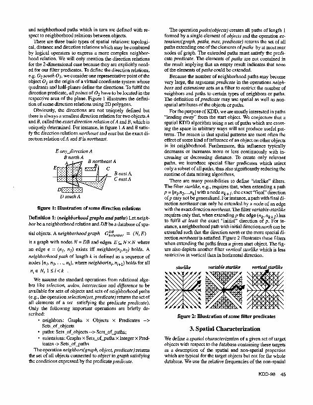
For the purpose of KDD, we are mostly interested in paths “leading away” from the start object. We conjecture that a spatial KDD algorithm using a set of paths which are cross- ing the space in arbitrary ways will not produce useful pat- terns. The reason is that spatial patterns are most often the effect of some kind of influence of an object on other objects in its neighborhood. Furthermore, this influence typically decreases or increases more or less continuously with in- creasing or decreasing distance. To create only relevant paths, we introduce special filter predicates which select only a subset of all paths, thus also significantly reducing the runtime of data mining algorithms.

There are many possibilities to define “starlike” filters. The filter starlike, e.g., requires that, when extending a path p = [q,n2,..., nk] with a node nk+I, the exact “final” direction of p may not be generalized. For instance, a path with final di- rection northeast can only be extended by a node of an edge with the exact direction northeast. The filter variable-starlike requires only that, when extending p the edge (nk, nk+l) has to fulfil at least the exact “initial” direction of p. For in- stance, a neighborhood path with initial direction north can be extended such that the direction north or the more special di- rection northeast is satisfied. Figure 2 illustrates these filters when extending the paths from a given start object. The fig- ure also depicts another filter vertical starlike which is less restrictive in vertical than in horizontal direction.

starlike vertical~turlike

figure 2: Illustration of some filter predicates

3. Spatial Characterization We define a spatial characterization of a given set of target objects with respect to the database containing these targets as a description of the spatial and non-spatial properties which are typical for the target objects but not for the whole database. We use the relative frequencies of the non-spatial

KDD-98 45

attribute values and the relative frequencies of the different object types as the interesting properties. For instance, dif-

attributes attributes -

(a) relative frequencies (b) relative frequencies in the database in the target regions

g 4 significance

t? Q E b (c) ratio of the frequencies

figure 3: Sample frequencies and differences

ferent object types in a geographic database are communi- ties, mountains, lakes, highways, railroads etc. To obtain a spatial characterization, we consider not only the properties of the target objects, but also the properties of their neigh- bors up to a given maximum number of edges in the neigh- borhood graph. Figure 3 depicts an example for the relative frequencies in the database as well as in the target regions and the ratio of these frequencies in comparison with the specified level of significance.

The task of spatial characterization is to discover the set of all tuples (attribute, value) and the set of all objects types for which the relative frequency in a set targets, extended by its

neighbors, is significantly different from the relative fre- quency in DB. A very frequent property present only in the neighborhood of very few of the targets would create mis- leading results. Therefore, we require that such a property must also have a significantly larger relative frequency in the neighborhood of many targets.

Definition 2: (spatial characterization): Let Gfzghbor be a neighborhood graph and targets be a subset of DB. Let freqS(prop) denote the number of occurrences of the proper- ty prop in the set s and let card(s) denote the cardinality of s. Thefrequency factor of prop with respect to targets and DB, denoted by fFzg,,,(prop), is defined as follows:

fargets(prop) freqDB(prop) f F$ets(ProP) = ‘raTd(targets) ’ card( DB)

Let significance and proportion be real numbers and let ma-neighbors be a natural number. Let neighbor+(s) denote the set of all objects reachable from one of the ele- ments of s by traversing at most i of the edges of the neigh- borhood graph G. Then, the task of spatial characterization is to discover each property prop and each natural number n I max-neighbors such that (1) the set objects = neighborsa(targets) as well as (2) the sets objects = neighborsE({ t}) for at least proportion many t E targets satisfy the condition:

2 significance f ftects(ProP) Or 1

5 significance

In point (1) the union of the neighborhood of all target ob- jects is considered simultaneously, whereas in point (2) the

characterization(graph Gf ; set of objects targets; real signifiance, proportion; integer mux-neighbors:

initialize the set of characterizations as empty; initialize the set of regions to targets; initialize n to 0; calculate frequencPB@rop) for all properties prop = (attribute, value); while n I max-neighbors do

for each attribute of DB and for the special attribute object type do for each value of attribute do

calculatefrequencyregions (prop) for property prop = (attribute, value); if f f)eBgions(ProP) 2 significance or (prop) I 11 significance then

add (Prop, It, f gfions f f)eBions

(prop) ) to the set characterizations; if n < max-neighbors then

for each object in regions do add neighbors( GrB , object, TRUE) to regions;

increment n by 1; extract all tuples (prop, n, f(prop)) from characterizations which are significant in at least proportion of the

regions with n extensions; return the rule generated from these characterizations;

figure 4: Algorithm spatial characterization

46 Ester

neighborhood of each target object is considered separately. The parameter proportion specifies the minimum confi- dence required for the characterization rules and the fre- quency factors of the properties provide a measure of their interestingness with respect to the given target objects.

Figure 4 presents the algorithm for discovering spatial characterizations. The parameter proportion is relevant only for the last step of the algorithm, i.e. for the generation of a rule. Note the importance of the parameter n (that is, the maximum number of edges of the neighborhood graph tra- versed starting from a target object) in the resulting charac- terizations. For example, a property may be significant when considering all neighbors which are reachable from one of the target objects via 2 edges of the neighborhood graph. However, the same property may not be significant when considering further neighbors if then the target regions are extended by objects for which the property is not frequent. The generated rule has the following format:

target * pl (nl, freq-facl) fi . . . A pk (nk, freq- fack). This rule means that for the set of all targets extended by

ni neighbors, the property pi isfreq-faci times more (or less) frequent than in the database.

4. Spatial Trend Detection We define a spatial trend as a regular change of one or more non-spatial attributes when moving away from a given start object o. We use neighborhood paths starting from o to mod- el the movement and we perform a regression analysis on the respective attribute values for the objects of a neighborhood path to describe the regularity of change. Since we are inter- ested in trends with respect to o, we use the distance from o as the independent variable and the difference of the at-

tribute values as the dependent variable(s) for the regression. The correlation of the observed attribute values with the val- ues predicted by the regression function yields a measure of confidence for the discovered trend.

(a) positive trend (b) negative trend (c) no trend

figure 5: Sample trends

In the following, we will use linear regression, since it is efficient and often the influence of some phenomenon to its neighborhood is either linear or may be transformed into a linear model, e.g. exponential regression. Figure 5 illus- trates a positive and a negative (linear) trend as well as a sit- uation where no significant (linear) trend is observed.

Definition 3: (spatial trend detection): Let g be a neighbor- hood graph, o an object (node) in g. and a be a subset of all non-spatial attributes. Let # be a type of function, e.g. linear or exponential, used for the regression and letfilter be one of the filters for neighborhood paths. Let min-conf be a real number and let min-length as well as mu-length be natural numbers. The task of spatial trend detection is to discover the set of all neighborhood paths in g starting from o and having a trend of type # in attributes a with a correlation of at least min-conf. The paths have to satisfy the filter and their length must be between min-length and max-length.

global-trend(graph g; object o; attribute a; type t; real min-conf, integer min-Zength,max-length; filtern initialize a list of paths to the set extensions(g, path(o), min-length, f3; initialize an empty set of observations; initialize the last-correlation and last-paths as empty; initialize first-pos to 1; initialize last-pos to min-length; while paths is not empty do

for each path in paths do for object fromfirst-pos of path to last-pos of path do

calculate diffas a(objec#) - a(o) and calculate dist as dis#(objec#,o); insert the tuple (difl, dist) into the set of observations;

perform a regression of type t on the set of observations; if abs(correlation) of the resulting regression function 2 min-conf then

set last-correlation to correlation and last-paths to paths; if the length of the paths < max-length then

replace the paths by the set extensions(g,paths, 1, fi; increment last-pos by 1; set first-pos to last-pos;

else set paths to the empty list; else return last-correlation and last-paths;

return the last correlation and last-paths;

figure 6: Algorithm global-trend

KDD-98 47

local-trends(graph g; object o; attribute a; type t; real min-conf, integer min-Zengthpzux-Zength; filters) initialize a list of paths to the set extensions(g, path(o), min-length, fl; initialize two empty sets of positive and negative trends; while paths is not empty do

initialize the set of observations as empty; remove the first element of paths and take it as path; for object from min-length& object of path to last object of path do

calculate di$fas a(object) - a(o) and calculate dist as dist(object,o); insert the tuple (di#,dist) into the set of observations;

I perform a regression of type t on the set of observations; if abs(correlation) of the resulting regression function 2 min-conf then

if correlation > 0 then insert the tuple (path, correlation) into the set of positive trends;

else insert the tuple (path, correlation) into the set of negative trends; if the length of path c max-length then

add the extensions(g,path,I, f) to the head of paths; return positive-trends and negative-trends;

figure 7: Algorithm local-trends

Definition 3 allows different specializations. Either the set of all discovered neighborhood paths (global trend) or each of its elements (local trend) must have a trend of the specified type.

Algorithm global-trend is depicted in figure 6. Beginning from o, it creates all neighborhood paths of the same length simultaneously - starting with min-length and continuing until max-length. The regression is performed once for each of these sets of all paths of the same length. If no trend of length I with correlation 2 min-conf is detected, then the path extensions of length Z+I, Z+Z, . . ., max-length are not creat- ed. The algorithm returns the significant spatial trend with the maximum length.

Algorithm local-trends is outlined in figure 7. This algo- rithm performs a regression once for each of the neighbor- hood paths with length 1 min-length and a path is only ex- tended further if it has a significant trend. The algorithm returns two sets of paths showing a significant spatial trend, a set of positive trends and a set of negative trends.

5. Performance Evaluation We implemented the database primitives on top of the com- mercial DBMS Illustra (Illustra 1997) using its 2D spatial data blade which offers R-trees. The advantage of this ap- proach is an easy and rather portable implementation. The disadvantage is that we cannot reduce the relatively large system overhead imposed by the underlying DBMS.

A geographic database on Bavaria was used for the exper- imental performance evaluation of our algorithms. The data- base contains the ATKIS 500 data (Bavarian State Bureau of Topography and Geodesy 1996) and the Bavarian part of the statistical data obtained by the German census of 1987, i.e. 2043 Bavarian communities with one spatial attribute (poly- gon) and 52 non-spatial attributes (such as average rent or rate of unemployment). Also included are spatial objects representing natural object like mountains or rivers and in-

48 Ester

Relation Bavarian Communities:

figure 8: Spatial and non-spatial attributes frastructure such as highways or railroads. The total number of spatial objects in the database then amounts to 6924. The relation communities is sketched in figure 8. This geograph- ic database may be used, e.g., by economic geographers to discover spatial rules on the economic power of communi- ties. We performed several sets of experiments to measure the performance of our characterization and spatial trend de- tection algorithms. Note, that the runtime of the algorithms is in general not dependent on the database size but on the size of the input and on the number of neighborhood opera- tions performed for the considered objects. This number de- pends on the average number of neighbors per object in the database which is an application dependent parameter. In

our geographic information system the average number of neighboring communities is approximately six.

5.1 Characterization The characterization algorithm usually starts with a small set of target objects, selected for instance by a condition on some non-spatial attribute(s) such as “rate of retired people = HIGH” (see figure 9, left). Then, the algorithms expands regions around the target objects, simultaneously selecting those attributes of the regions for which the distribution of values differs significantly from the distribution in the whole database (figure 9, right). In the last step of the algorithm, a characterization rule is generated describing the target re- gions (figure 9, bottom). In this example, not only some non-spatial attributes but also the neighborhood of moun- tains (after three extensions) are significant for the charac- terization of the target regions.

target objects maximally expanded regions

rule characterizing the target objects object has high rate of retired people 3

apartments per building = very low (0,g.l) A rate of foreigners = very low (0,8.9) A rate of academics = medium (0, 6.3) A

average size of enterprises = very low (0,5.8) A

object type = mountain (3,4.1)

figure 9: Characterizing wrt. high rate of retired people

Table 1 reports the efficiency of our spatial characteriza- tion algorithm. The numbers are calculated as the average over all start objects for several experiments with different target sets.

5.2 Trend Detection Spatial trends describe a regular change of non-spatial at- tributes when moving away from a start object o. The two al- gorithms above may produce different patterns of change for the same start object o.

The existence of a global trend for a start object o indi- cates that if considering all objects on all paths starting from o the values for the specified attribute(s) in general tend to increase (decrease) with increasing distance. Figure 10 (left) depicts the result of algorithm global-trend for the attribute “average rent” and the city of Regensburg as a start object.

Algorithm local-trends detects single paths starting from an object o and having a certain trend. The paths starting from o may show different pattern of change, e.g., some trends may be positive while the others may be negative. Figure 10 (right) illustrates this case for the attribute “aver- age rent” and the city of Regensburg as a start object.

The spatial objects within a trend region, i.e. either the start objects or the objects forming the paths, may be the subject of further analysis. For instance, algorithm global- trend may detect regions showing a certain global trend, and algorithm local-trends then finds within these regions some paths having the inverse trend (see figure 10). Then, we may try to find an explanation for those “inverse” paths. Another possibility is to detect “centers” for a given attribute first (using algorithm global-trend) and then apply our character- ization algorithm to the centers to find their common proper- ties. An example for this approach is presented in more de- tail in section 5.3.

Global trend (min-conk0.7) Local trends (tin-confi0.9)

+ direction of decreasing attribute values

figure 10: Visualization of trends for attribute “average rent” starting from the city of Regensburg

For our performance test we applied both algorithms to the Bavaria database varying min-con.dence from 0.6 to 0.8 for the attribute “average rent” and linear type of regression. The predicate intersects was used as the neighborhood rela- tion to define the graph. The filter vertical starlike for paths was used because due to our domain knowledge we expect- ed the most significant trends in north-south direction. The length of the paths was restricted by min-length = 4 and max- length = 7.

Table 2 reports the performance results for the algorithms global-trend and local-trends. The average numbers shown were calculated over all start objects.

Table 1: Performance of spatial characterization

KDD-98 49

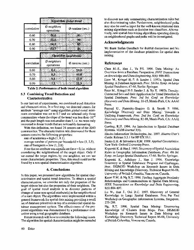
correlation 0 neighbors operations 0 runtime (sec.)

1 correlation 11 ( 0 runtime (sec.)

Table 2: Performance of both trend algorithm

5.3 Combining Trend Detection and Characterization

In our last set of experiments, we combined trend detection and characterization. In a first step, we detected centers for attribute “average rent” using algorithm global-trend: mini- mum correlation was set to 0.7 and we selected only those communities where the slope of the trend was less than - 1 OS4 and the path length was not smaller than 5, i.e. we were only interested in linear trends that are noticeably decreasing.

With this definition, we found 24 centers out of the 2043 communities. The characterization rule discovered for these centers contains the following properties:

rate of academics = high (1,9. l), average number of persons per household = low (1,2.5), rate of foreigners = low (1,2.8). Note that no attribute was significant for n = 0, i.e. without

considering the neighborhood of the target object. Only if we extend the target regions by one neighbor, we can see some characteristic properties. Thus, this result could not be found by a non-spatial characterization algorithm.

6. Conclusions In this paper, we presented new algorithms for spatial char- acterization and spatial trend detection. To obtain a spatial characterization, we consider not only the properties of the target objects but also the properties of their neighbors. The goal of spatial trend analysis is to discover patterns of change of some non-spatial attribute(s) in the neighborhood of a start object. The algorithms were implemented within a general framework for spatial data mining providing a small set of database primitives on top of a commercial spatial da- tabase management system. The effectiveness of the pro- posed algorithms was demonstrated by a performance eval- uation using a real geographic database.

Future research will have to consider the following issues. The algorithm for spatial characterization might be extended

to discover not only summarizing characterization mies but also discriminating rules. Furthermore, neighborhood paths may also be used as input for the well-known relational data mining algorithms such as decision tree classifiers. Alterna- tively, new spatial data mining algorithms operating directly on neighborhood graphs and paths will be investigated.

Acknowledgments We thank Stefan Gundlach for fruitful discussions and his implementation of the database primitives for spatial data mining.

References Chen M.-S., Han J., Yu P.S. 1996. Data Mining: An Overview from a Database Perspective. ZEEE Transactions on Knowledge and Data Engineering, 8(6): 866-883. Ester M., Kriegel H.-P. & Sander J. 1997a. Spatial Data Mining: A Database Approach. Proc. 5th Znt. Symp. on Large Spatial Databases, 47-66, Berlin: Springer. Ester M., Kriegel H-P, Sander J. & Xu X. 1997b. Density- Connected Sets and their Application for Trend Detection in Spatial Databases. Proc. 3rd Znt. Conf on Knowledge Discovery and Data Mining, 10-15, Menlo Park, CA: AAAI Press. Fayyad U., Piatetsky-Shapiro G. & Smyth P. 1996. Knowledge Discovery and Data Mining: Towards a Unifying Framework Proc. 2nd Znt. Conjc: on Knowledge Discovery and Data Mining, 82-88, Menlo Park, CA: AAAI Press. Gueting, R.H. 1994. An Introduction to Spatial Database Systems. VLDB Journal 3(4). Illustra Information Technologies, Inc. 1997. Illustra User’s Guide. Release 3.3.1 for HP UX 10.1. Isaaks E.H. & Srivastava R.M. 1989. Applied Geostatistics. New York: Oxford University Press. Koperski K. & Han J. 1995. Discovery of Spatial Association Rules in Geographic Information Databases. Proc. 4th Znt. Symp. on Large Spatial Databases, 47-66. Berlin: Springer. Koperski K., Adhikary J., Han J. 1996. Knowledge Discovery in Spatial Databases: Progress and Challenges. Proc. SIGMOD Workshop on Research Issues in Data Mining and Knowledge Discovery, Technical Report 96-08, University of British Columbia, Vancouver, Canada. Knorr E.M. & Ng R.T. 1996. Finding Aggregate Proximity Relationships and Commonalities in Spatial Data Mining. IEEE Transactions on Knowledge and Data Engineering, 8(6):884-897. Lu W., Han J., Ooi B.C. 1993. Discovery of General Knowledge in Large Spatial Databases. Proc. Far East Workshop on Geographic Information Systems, Singapore, 275-289. Ng, R.T. 1996. Spatial Data Mining: Discovering Knowledge of Clusters from Maps. Proc. SIGMOD Workshop on Research Issues in Data Mining and Knowledge Discovery, Technical Report 96-08, University of British Columbia, Vancouver, Canada.

50 Ester