F73DA2 INTRODUCTORY DATA ANALYSIS ANALYSIS OF VARIANCE
68
F73DA2 F73DA2 INTRODUCTORY DATA ANALYSIS INTRODUCTORY DATA ANALYSIS ANALYSIS OF VARIANCE ANALYSIS OF VARIANCE
-
Upload
wynter-graves -
Category
Documents
-
view
29 -
download
2
description
F73DA2 INTRODUCTORY DATA ANALYSIS ANALYSIS OF VARIANCE. regression: x is a quantitative explanatory variable. type is a qualitative variable (a factor). Illustration. Company 1: 36 28 32 43 30 21 33 37 26 34 Company 2: 26 21 31 29 27 35 23 33 Company 3: - PowerPoint PPT Presentation
Transcript of F73DA2 INTRODUCTORY DATA ANALYSIS ANALYSIS OF VARIANCE

F73DA2 F73DA2 INTRODUCTORY DATA ANALYSISINTRODUCTORY DATA ANALYSIS
ANALYSIS OF VARIANCEANALYSIS OF VARIANCE
1.0 1.5 2.0 2.5 3.0
20
25
30
35
40
45
50
x
y
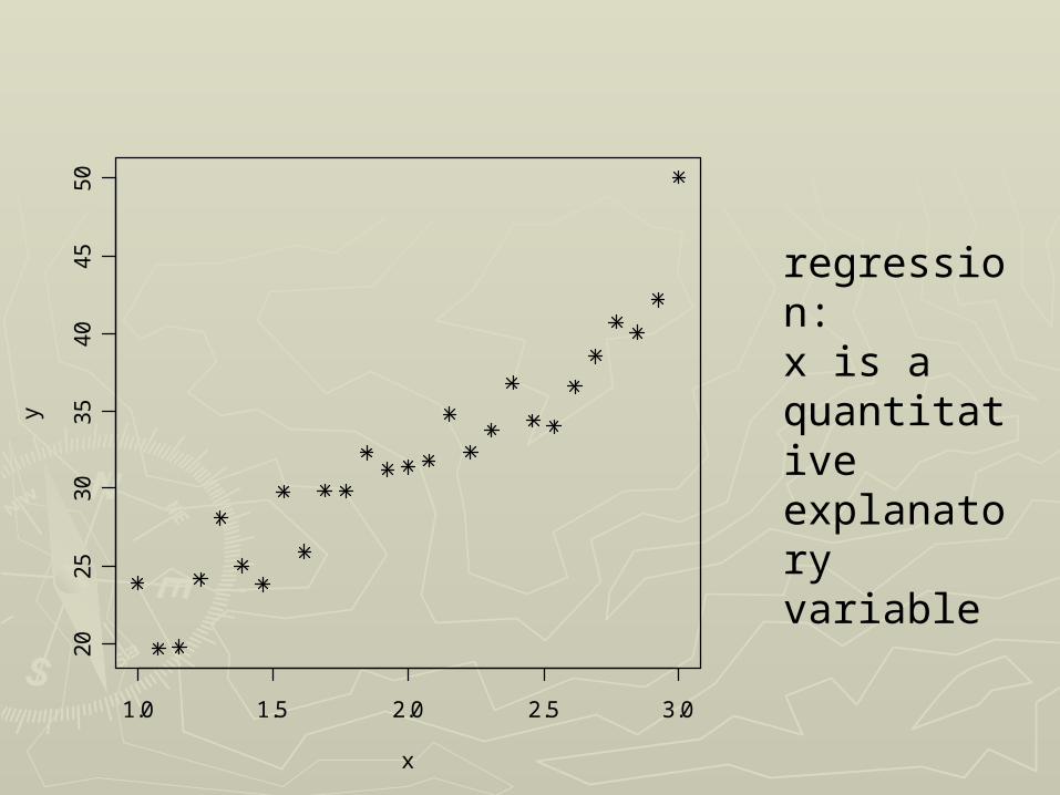
regression:x is a quantitativeexplanatory variable

1.0 1.5 2.0 2.5 3.0
20
25
30
35
40
45
50
type
y
type is a qualitativevariable (a factor)

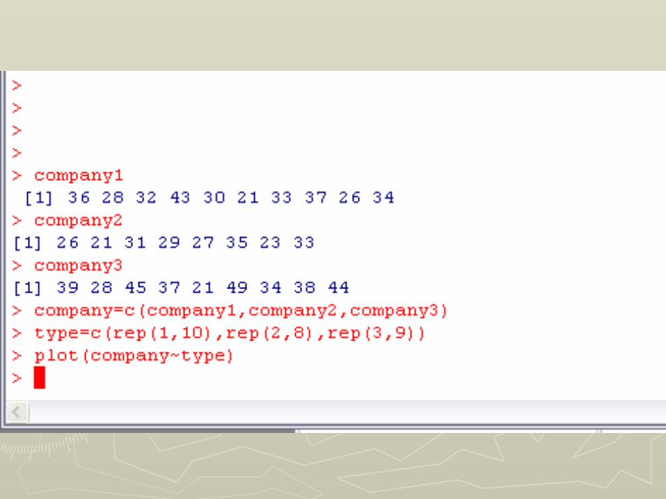
Company 1: Company 1:
36 28 32 43 30 21 33 37 26 3436 28 32 43 30 21 33 37 26 34
Company 2: Company 2:
26 21 31 29 27 35 23 3326 21 31 29 27 35 23 33
Company 3: Company 3:
39 28 45 37 21 49 34 38 4439 28 45 37 21 49 34 38 44
IllustrationIllustration

1.0 1.5 2.0 2.5 3.0
20
25
30
35
40
45
50
company
sum

Explanatory variable qualitativei.e. categorical - a factor
Analysis of variance linear models for comparative experiments

1.0 1.5 2.0 2.5 3.0
20
25
30
35
40
45
50
type
com
pa
ny

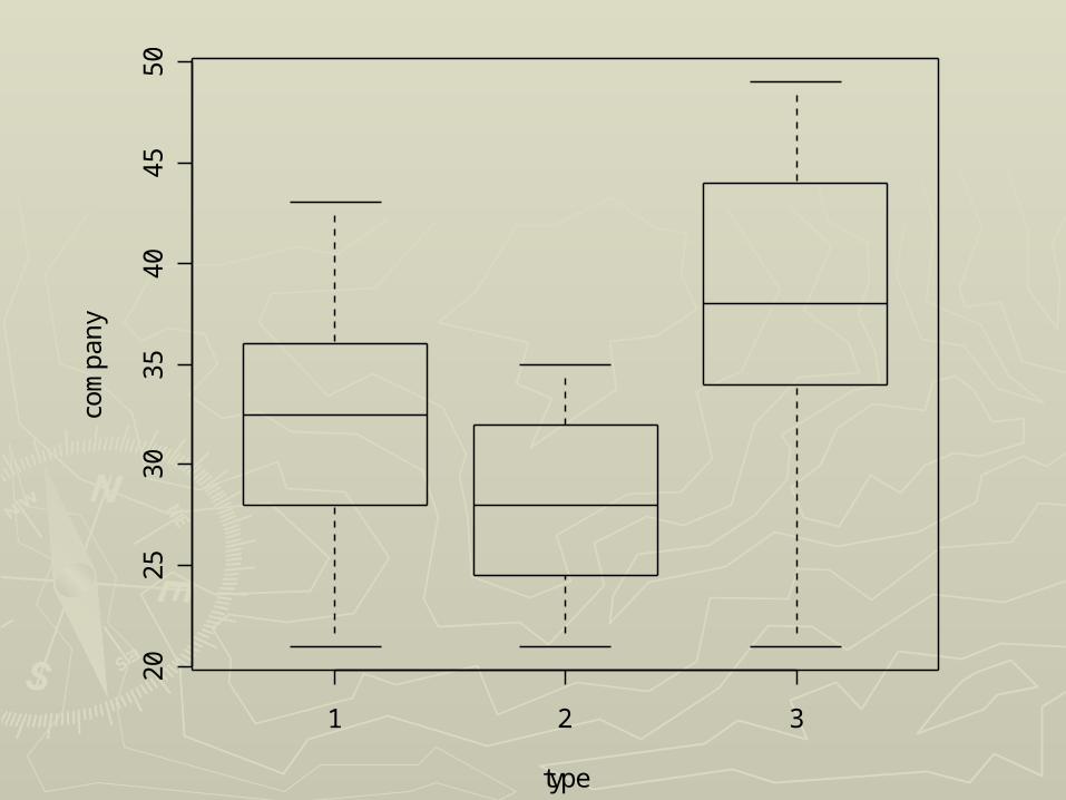
►The display is different if “type” is The display is different if “type” is declared as a factor. declared as a factor.
Using Factor CommandsUsing Factor Commands

1 2 3
20
25
30
35
40
45
50
type
com
pa
ny
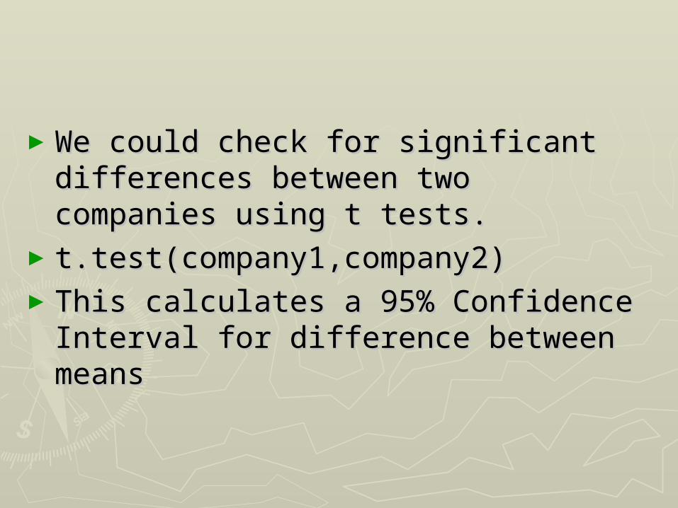
►We could check for significant We could check for significant differences between two companies differences between two companies using t tests.using t tests.
►t.test(company1,company2)t.test(company1,company2)►This calculates a 95% Confidence This calculates a 95% Confidence
Interval for difference between meansInterval for difference between means

Includes 0 so no significant difference
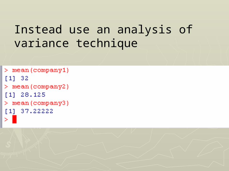
Instead use an analysis of variance technique

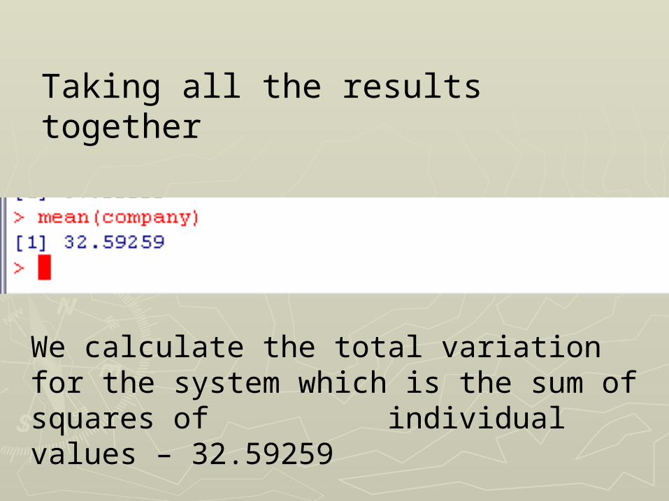
Taking all the results together
Taking all the results together
We calculate the total variation for the system which is the sum of squares of individual values – 32.59259


►We can also work out the sum of We can also work out the sum of squares within each companysquares within each company
This sums to 1114.431

►The total sum of squares of the The total sum of squares of the situation must be made up of a situation must be made up of a contribution from variation WITHIN the contribution from variation WITHIN the companies and variation BETWEEN the companies and variation BETWEEN the companies.companies.
►This means that the variation between This means that the variation between the companies equals 356.0884the companies equals 356.0884

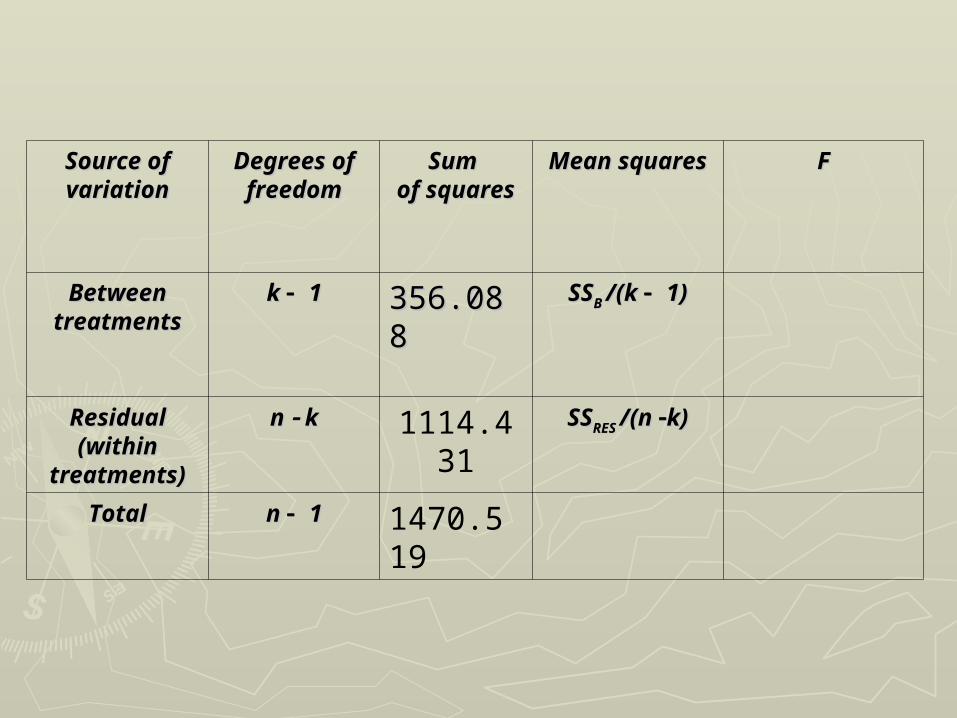
►This can all be shown in an analysis of This can all be shown in an analysis of variance table which has the format:variance table which has the format:

Source of Source of variationvariation
Degrees of Degrees of freedomfreedom
Sum Sum of of
squaressquares
Mean Mean squaressquares
FF
Between Between treatmentstreatments
k k 11 SSSSBB SSSSB B /(k /(k 1)1)
ResidualResidual(within (within
treatments)treatments)
n n k k SSSSRESRES SSSSRES RES /(n /(n k)k)
TotalTotal n n 11 SSSSTT
Source of Source of variationvariation
Degrees of Degrees of freedomfreedom
Sum Sum of of
squaressquares
Mean Mean squaressquares
FF
Between Between treatmentstreatments
k k 11 356.088356.088 SSSSB B /(k /(k 1)1)
ResidualResidual(within (within
treatments)treatments)
n n k k 1114.431
SSSSRES RES /(n /(n k)k)
TotalTotal n n 11 1470.519
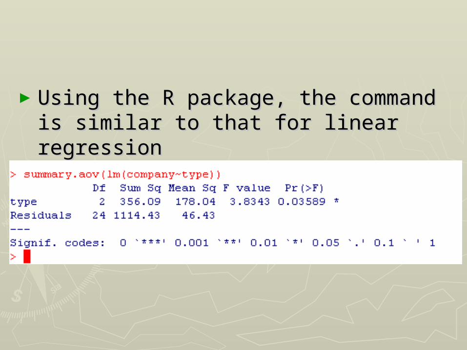
►Using the R package, the command is Using the R package, the command is similar to that for linear regressionsimilar to that for linear regression
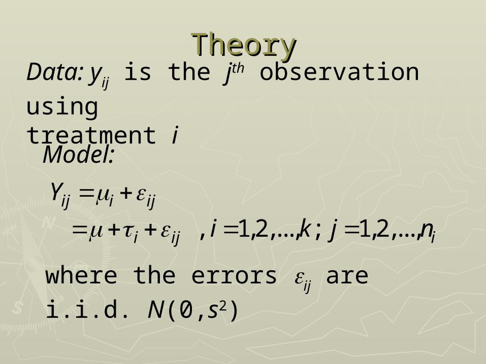
Data: yij is the jth observation using
treatment i
where the errors ij are i.i.d. N(0,s2)
, 1,2,..., ; 1,2,...,ij i ij
i ij i
Y
i k j n
Model:
TheoryTheory

The response variables Yij are independent
Yij ~ N(µ + τi , σ2)
Constraint:
0i ii
n

2
1 1
1 1 1
2 , 2
i
i i
nk
ij ii j
n nk
ij i ij ii j ji
S y
S Sy y
Derivation of least-squares estimators

Normal equations for the estimators:ˆ ˆ ˆand
with solutionˆ ˆ,
i i i i
i i
y n y n n
y y y
The fitted values are the treatment means
iij YY

Partitioning the observed total variation
2 2 2
ij ij i i ii j i j i
y y y y n y y
SST = SSB + SSRES
SST SSRES SSB
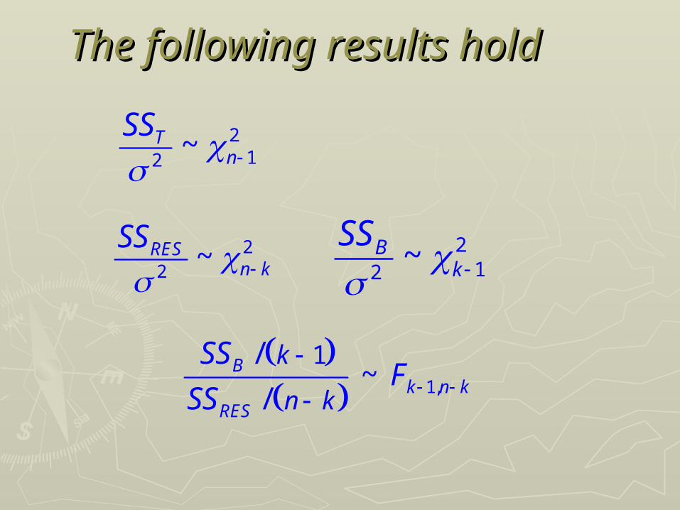
The following results holdThe following results hold
212
~Tn
SS
22
~RESn k
SS
212
~Bk
SS
1,
1/~
/B
k n kRES
k
n k
SSF
SS

1
2
3
ˆ 880/ 27 32.593ˆ 320/10 880/ 27 0.593,
ˆ 225/8 880/ 27 4.468
ˆ 335/9 880/ 27 4.630
Back to the example
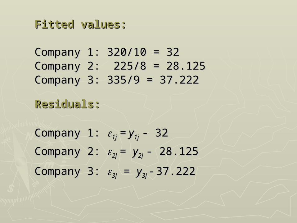
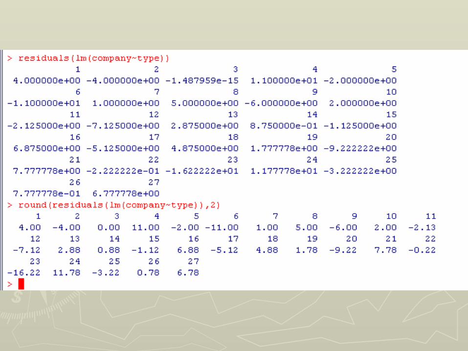
Fitted values:Fitted values:
Company 1: 320/10 = 32Company 1: 320/10 = 32Company 2: 225/8 = 28.125Company 2: 225/8 = 28.125Company 3: 335/9 = 37.222Company 3: 335/9 = 37.222
Residuals:Residuals:
Company 1: Company 1: 1j1j = y = y1j1j - 32- 32
Company 2: Company 2: 2j2j = = yy2j2j - 28.125- 28.125
Company 3: Company 3: 3j3j = = yy3j3j - - 37.22237.222

SSSSTT = 30152 – 880 = 30152 – 88022/27 = 1470.52/27 = 1470.52
SSSSBB = (320 = (32022/10 + 225/10 + 22522/8 + 335/8 + 33522/9) – 880/9) – 88022/27/27
= 356.09= 356.09
SSSSRESRES = 1470.52 – 356.09 = 1114.43 = 1470.52 – 356.09 = 1114.43

ANOVA tableANOVA table
Source of Degrees of Sum Mean FSource of Degrees of Sum Mean Fvariationvariation freedom of squares squares freedom of squares squares
Between Between 2 356.09 178.04 2 356.09 178.04 3.833.83
treatmentstreatmentsResidualResidual 2424 1114.43 46.44 1114.43 46.44
Total Total 26 1470.5226 1470.52
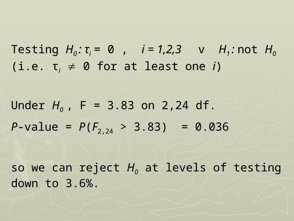
Testing Testing HH0 0 : τ: τii = 0 , = 0 , i = 1,2,3 i = 1,2,3 v v HH1 1 : : not not HH00
(i.e. τ(i.e. τii 0 for at least one 0 for at least one ii))
Under Under HH00 , F = 3.83 on 2,24 df. , F = 3.83 on 2,24 df.
PP-value = -value = PP((FF2,242,24 > 3.83) = 0.036 > 3.83) = 0.036
so we can reject so we can reject HH00 at levels of testing at levels of testing
down to 3.6%.down to 3.6%.
Conclusion
Results differ among thethree companies (P-value 3.6%)

The fit of the model can be investigated by examining the residuals:
the residual for response yij is
iijijij yye
this is just the difference between the response
and its fitted value (the appropriate sample mean).

Plotting the residuals in various ways may reveal
● a pattern (e.g. lack of randomness, suggesting that an additional, uncontrolled factor is present)
● non-normality (a transformation may help)
● heteroscedasticity (error variance differs among treatments – for example it may increase with treatment mean: again a transformation – perhaps log - may be required)

1.0 1.5 2.0 2.5 3.0
20
25
30
35
40
45
50
type
com
pa
ny
1 2 3
20
25
30
35
40
45
50
type
com
pa
ny

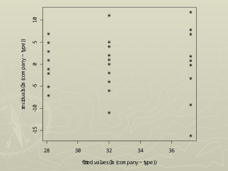
► In this example, samples are small, In this example, samples are small, but one might question the validity of but one might question the validity of the assumptions of normality the assumptions of normality (Company 2) and homoscedasticity (Company 2) and homoscedasticity (equality of variances, Company 2 v (equality of variances, Company 2 v Companies 1/3). Companies 1/3).

0 5 10 15 20 25
-15
-10
-50
51
0
Index
resi
du
als
(lm
(co
mp
an
y ~
typ
e))
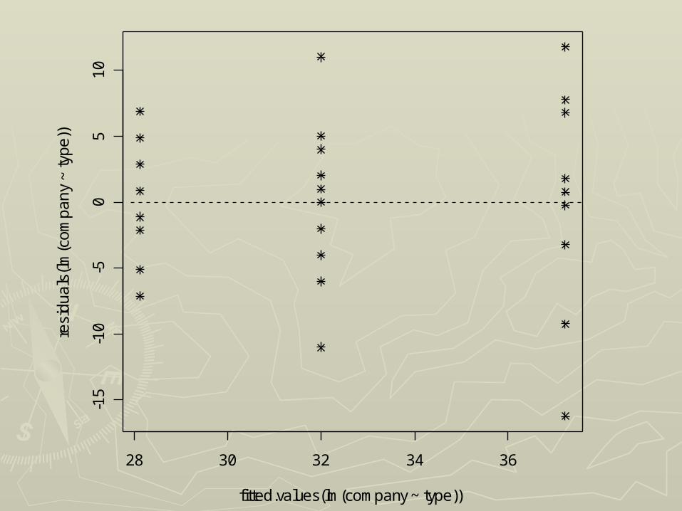
► plot(residuals(lm(company~type))~ plot(residuals(lm(company~type))~ fitted.values(lm(company~type)),pch=fitted.values(lm(company~type)),pch=8)8)
28 30 32 34 36
-15
-10
-50
51
0
fitted.values(lm(company ~ type))
resi
du
als
(lm
(co
mp
an
y ~
typ
e))

► plot(residuals(lm(company~type))~ plot(residuals(lm(company~type))~ fitted.values(lm(company~type)),pch=fitted.values(lm(company~type)),pch=8)8)
► abline(h=0,lty=2)abline(h=0,lty=2)
28 30 32 34 36
-15
-10
-50
51
0
fitted.values(lm(company ~ type))
resi
du
als
(lm
(co
mp
an
y ~
typ
e))

► It is also possible to compare with an It is also possible to compare with an analysis using “type” as a qualitative analysis using “type” as a qualitative explanatory variableexplanatory variable
►type=c(rep(1,10),rep(2,8),rep(3,9))type=c(rep(1,10),rep(2,8),rep(3,9))►No “factor” commandNo “factor” command

1.0 1.5 2.0 2.5 3.0
20
25
30
35
40
45
50
type
com
pa
ny
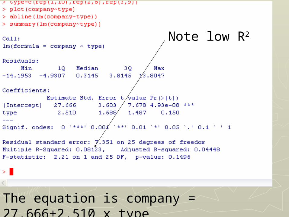
The equation is company = 27.666+2.510 x type
Note low R2

A B C D E F
05
10
15
20
25
spray
cou
nt

5 10 15
-50
51
0
fitted.values(lm(count ~ spray))
resi
du
als
(lm
(co
un
t ~ s
pra
y))

Example
A school is trying to grade 300 different scholarship applications. As the job is too much work for one grader, 6 are used.

Example
A school is trying to grade 300 different scholarship applications. As the job is too much work for one grader, 6 are used. The scholarship committee would like to ensure that each grader is using the same grading scale, as otherwise the students aren't being treated equally. One approach to checking if the graders are using the same scale is to randomly assign each grader 50 exams and have them grade.

To illustrate, suppose we have just 27 tests and 3 graders (not 300 and 6 to simplify data entry). Furthermore, suppose the grading scale is on the range 1-5 with 5 being the best and the scores are reported as:
grader 1 4 3 4 5 2 3 4 5
grader 2 4 4 5 5 4 5 4 4
grader 3 3 4 2 4 5 5 4 4

The 5% cut off for F distribution with 2,21 df is 3.467. The null hypothesis cannot be rejected. No difference between markers.

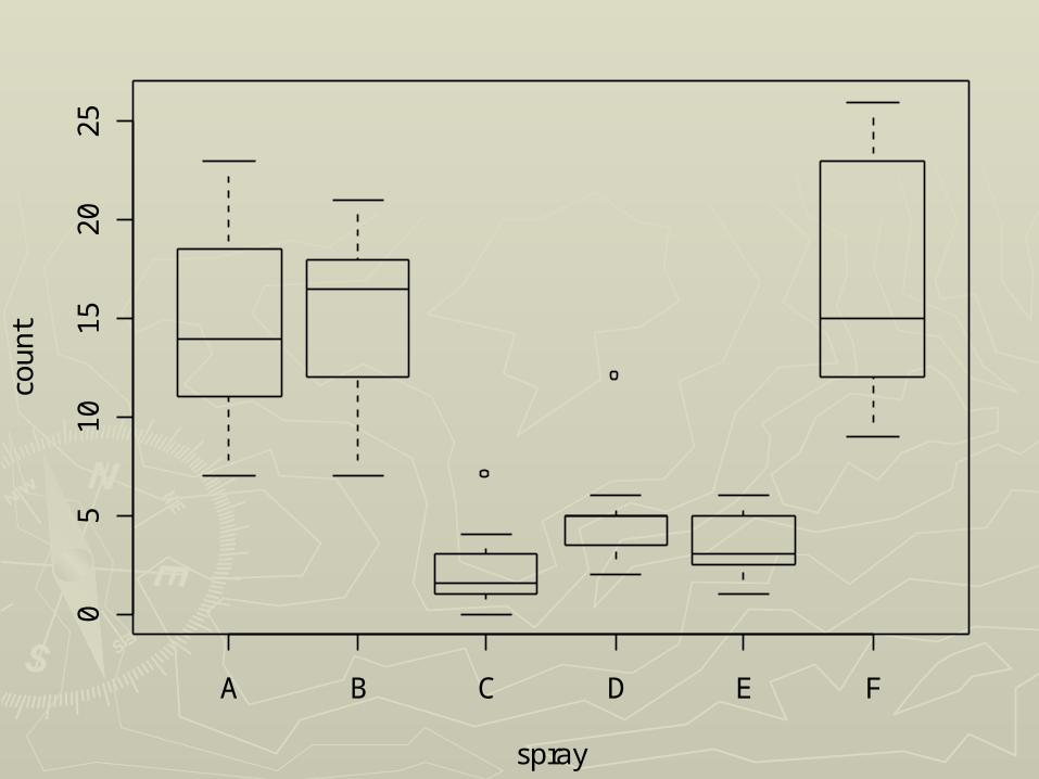
Class I II III IV V VI
151 152 175 149 123 145
168 141 155 148 132 131
128 129 162 137 142 155
167 120 186 138 161 172
134 115 148 169 152 141
Another Example

Source of variation
df Sum of squares
Mean squares
F
Between treatments
5 3046.7 609.3 2.54
Residual 24 5766.8 240.3
Total 29 8813.5

120 130 140 150 160 170 180
12
34
56
premium
com
pa
nyn
um
be
r

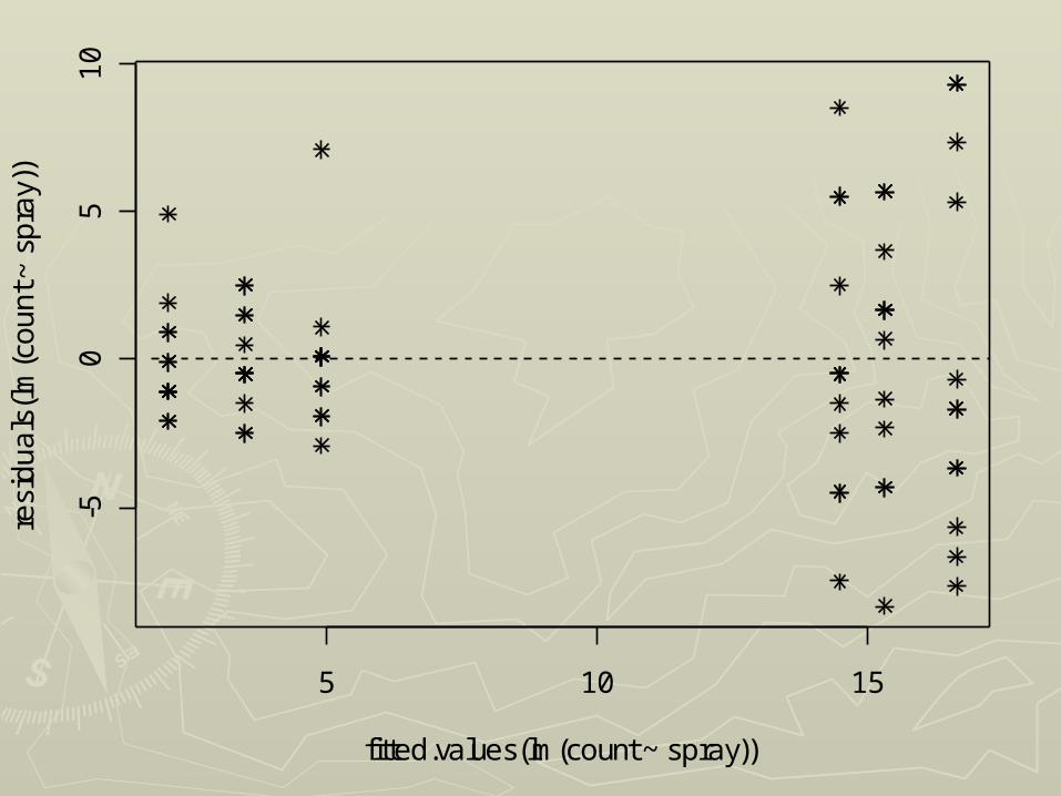
Normality and homoscedasticity (equality of variance) assumptions both seem reasonable

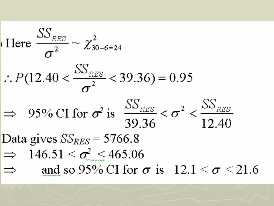
We now wish to Calculate a 95% confidence interval for the underlying common standard deviation , using
SSRES/ 2
as a pivotal quantity with a 2 distribution.

It can easily be shown that the class III has the largest value of 165.20 and that Class II has the smallest value of 131.40
Consider performing a t test to compare these two classes


There is no contradiction between this and the ANOVA results.
It is wrong to pick out the largest and the smallest of a set of treatment means, test for significance, and then draw conclusions about the set.Even if H0 : " all equal" is true, the sample means would differ and the largest and smallest sample means perhaps differ noticeably.