Extend sim 01
31
© Copyright 2010 Jeffrey Strickland, Ph.D. Discrete Event Simulation with ExtendSim Lesson 1 Missile Defense Agency Directorate of Modeling and Simulation Verification, Validation, and Accreditation
-
Upload
jeffrey-strickland-phd-cmsp-asep -
Category
Engineering
-
view
353 -
download
8
Transcript of Extend sim 01

© Copyright 2010 Jeffrey Strickland, Ph.D.
Discrete Event Simulation with ExtendSim
Lesson 1
Missile Defense Agency
Directorate of Modeling and Simulation
Verification, Validation, and Accreditation

© Copyright 2007 Dr. Jeffrey Strickland
What we’ll do
Lesson 1: Introduce Simulation modeling and
Discrete Event Simulation
Lesson 2: Introduce ExtendSim modeling and explore
a single-server queue model (MM1)
Analytic solution
Simulation solution
Inherent problems and DOE
Lesson 3: Construct a bank lobby model (several
versions: basic, a variety of resourcing methods,
hierarchical, and with animation)
Lesson 4: Build a simple BMDS End-to-End model

© Copyright 2007 Dr. Jeffrey Strickland
Lesson 1 Learning Objectives
Learn about the specification of a Discrete Event Simulation
(DES)
Distinguish a DES from other simulations
Learn about basic queuing processes and problems associated
with simulating them
Learn how to use appropriate statistical method to validate a
simple queuing model
Learn how to model a simple queuing problem in Extend
Learn how to design a simulation experiment and analyze the
results
Learn how to build basic and complex hierarchical models
Learn how to construct basic model animation
Learn how to build customized Extend blocks

© Copyright 2007 Dr. Jeffrey Strickland
Extend Models
It would be nice to model people returning to the moon, from
and end-to-end perspective, but it would take us a few years to
do so.
Reality: we have three days to learn about DES and Extend
Our models will be simple enough to build in three days, yet
complex enough to demonstrate many of the modeling
constructs and methodologies of the former
Resource pools, queues, and resource controls
Multiple random variate inputs and input tables for arrival
processes and service processes
Mixed modeling blocks (DES, Generic, Utility, etc.)
Hierarchical modeling
User interfaces and Notebook utility
Customized block development

© Copyright 2007 Dr. Jeffrey Strickland
Bank Model
Hierarchical modeling
Statistics collection
Buttons
Notebooks
Ghost Connectors
Multiple random inputs

© Copyright 2007 Dr. Jeffrey Strickland
Circuit Card Assembly
Multiple queues
Multiple services
Parallel servises
Serial services
Conveyer belts
Batching

© Copyright 2007 Dr. Jeffrey Strickland
Transportation
Labor pools
Task completion delays
Transferring goods
Transporting goods

© Copyright 2007 Dr. Jeffrey Strickland
Different Kinds of Simulation
Monte Carlo SimulationEstimate stochastic, static model quantities that are difficult to
compute by exact computations. A scheme employing random
numbers which is used for solving certain stochastic problems
where the passage of time plays no substantive role.
1
Dynamic SimulationDynamic system simulations observe the behavior of the
system models over time. The time advance mechanism used
here include continuous, discrete time, and discrete event.
2
Differential Equation System Specification (DESS)2a
Discrete Time System Specification (DTSS)2b
Discrete Event System Specification (DEVS)2b

© Copyright 2007 Dr. Jeffrey Strickland
Discrete-Event Simulation
Estimate stochastic, dynamic, and discrete model outputs. A scheme for modeling a system as it evolves over time by a representation in which state variables change instantaneously at separate points in time.
In simple terms, DEVS describes how a system with discrete flow units or jobs evolves over time.
Technically, this means that a computer tracks how and when state variables, such as queue lengths and resource availability, change over time.
State variables change as the result of an event (or discrete event) occurring in the system.
A characteristic is that discrete-event models focus only on the time instances when these discrete events occur.
This feature allows for significant time compression because it makes possible to skip through all time segments between events when the state of the system remains unchanged.

© Copyright 2007 Dr. Jeffrey Strickland
Formalized by Bernard Zeigler, University of Arizona, 1976 & 1990, 2000 [see references]
Provides a means of specifying a mathematical model of a system
Fundamental components
States
Inputs
Outputs
Transform functions
Time base
Discrete Event Simulation
© Copyright 2007 Dr. Jeffrey Strickland
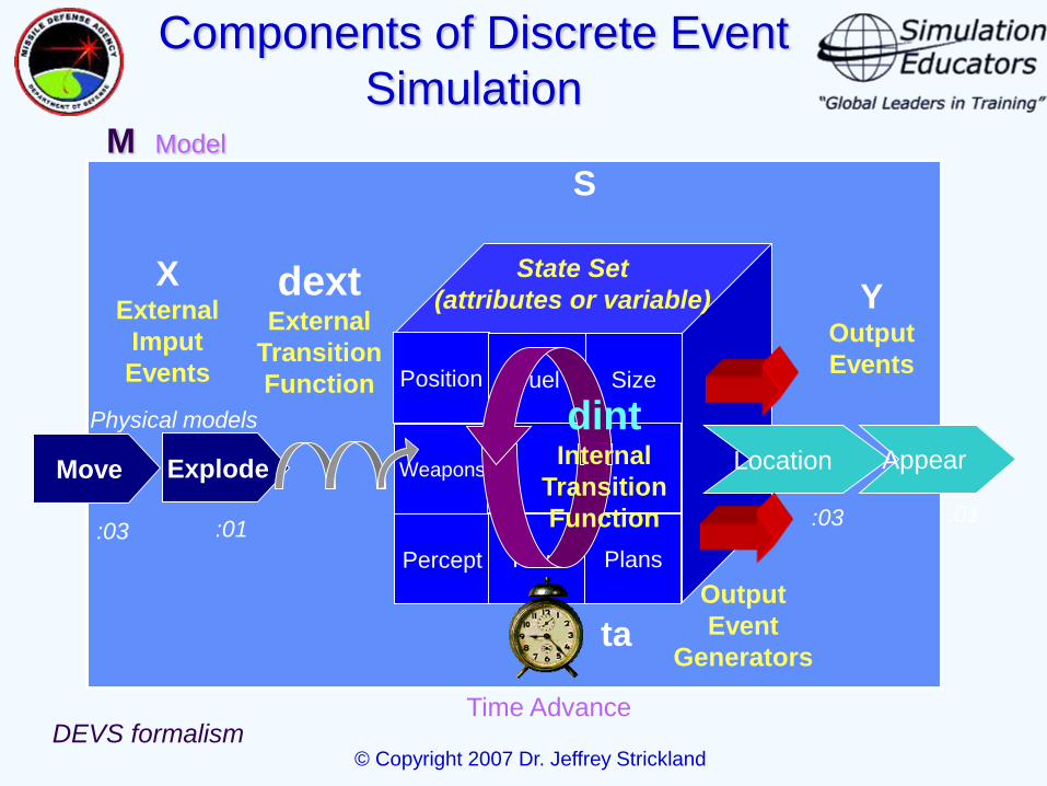
State Set
(attributes or variable)
Position Fuel Size
Weapons Health Strength
Percept Team Plans
S
Location Appear
YOutput
Events
Output
Event
Generators
Time Advance
ta
M Model
:03 :01
dintInternal
Transition
Function
Move Explode
XExternal
Imput
Events
:03 :01
Physical models
dextExternal
Transition
Function
DEVS formalism
Components of Discrete Event
Simulation

© Copyright 2007 Dr. Jeffrey Strickland
Basic System Specification
Formalisms
Discrete Event System Specification (DEVS)
DEVS = (X, Y, S, δext, δint, λ, ts)
X is the set of inputs
Y is the set of outputs
S is the set of sequential states
δext: Q X S is the set of external state transition function
δint: S S is the set of internal state transition function
λ: S Y is the output function that maps
ts: S o+ is the time advance function
Q = {(s,e)|sS, 0 < e < ta(s)} is the set of total states
Discrete Time System Specification (DTSS)
Differential Equation System Specification (DESS)

© Copyright 2007 Dr. Jeffrey Strickland
Basic Definitions
System State: a collection of variables containing all
information necessary to operate the model and record relevant
change in it over time.
Discrete-event dynamic system: system where the system
state change only at discrete points in time, which mark the
occurrence of an event.
Event: any occurrence that causes an instantaneous change in
the system state.
Arrival
Begin service
End service

© Copyright 2007 Dr. Jeffrey Strickland
Ordering Components
Event Scheduling
Events are generated and scheduled for the future
Event Queue Processing
Activity Scanning
Independent modules waiting to be executing
Sequential Model Execution
Process Interaction
Control each object through actions until delayed
Object List Processing

© Copyright 2007 Dr. Jeffrey Strickland
Event Scheduling
Need a mechanism to increment time by a variable amount between events.
Must be able to sequence events according to the time of occurrence and apply the associated transition function or event routine to make changes to the system state.
Accomplished by creating an event notice for each occurrence when its future time is determined.
Requires at least two items of information:
The actual time the event will occur
The type of event that is scheduled to occur
Event notices are stored in a list called the event list—ordered by time of occurrence.
The process of creating an event notice, recording the necessary information about the event, and placing it in the event list is called scheduling the event.

© Copyright 2007 Dr. Jeffrey Strickland
The System Clock
The system clock is a special system variable that holds the current system time.
The simulation progresses through time in the following way:
The first event notice on the event list is selected.
The system clock is set to the event time on this event notice.
Then the event routine for this type of event is executed to produce the appropriate changes in the system state for this type of event.
Finally, the event notice is discarded.
This process repeats until the event list is empty or some other signal is given to stop the simulation.
The routine that implements this process is called the timing routine—the heart of discrete-event simulation.

© Copyright 2007 Dr. Jeffrey Strickland
Model Development
The essence of modeling discrete-event simulation is to
determine:
1. what variables or components are needed to
adequately represent the systems state,
2. what events are needed to represent the system
changes, and
3. what state changes occur within each event,
including the details of which events are
schedules and when are they scheduled.
This is usually and iterative process.
There is no one unique model that represents a system.

© Copyright 2007 Dr. Jeffrey Strickland
Monte Carlo Theory
Random numbers are used to drive statistical models of processes and to make decisions.
The core of these algorithms is the uniformly distributed number between zero and one.
A series of independent and identically distributed numbers in the range from 0 to 1
Written as IID U(0,1)
Deterministic mathematical algorithms generate a series of numbers that appear random
X(n) = (ax(n-1) + c)mod(m)
U(0,1) = x(n)/MAX(m)
Random methods tend to generate very skewed sequences of numbers.

© Copyright 2007 Dr. Jeffrey Strickland
Random Variates
Uniform random numbers drive the selection values from other distributions (random variates)
Inverse Transform Methods assign the U(0,1) number as the Y-axis and traces it back to the X value through the desired cumulative distribution function.
Acceptance-Rejection Methods use an intermediate function to simplify the selection of numbers and maintain random selection.
Composition Methods decompose the distribution into a summed series of simpler distributions.

© Copyright 2007 Dr. Jeffrey Strickland
Characteristic Statistical Distributions
Statistical
Distribution
Potential Application
Uniform Source of random numbers between 0 and 1
Probability of Kill or Detection
Exponential Interarrival times of customers at a constant rate
Gamma Time to serve a customer
Weibull Time to failure for a piece of equipment
Normal Errors on the impact point of a bomb
Beta Proportion of defective items in a shipment
Bernoulli Success or failure of a specific experiment
Poisson Number of items in a batch of random size
Lognormal Task times with right-skewed distributions
Empirical Curves custom fitted to collected data

© Copyright 2007 Dr. Jeffrey Strickland
Output Analysis to Verify the Model
Finding the true distribution among events being generated of
time
Finite-Horizon Simulations start idle and execute to defined
terminating event
Eliminates the effects associated with starting the system
Steady-State Simulations run for long period of time until the
parameters achieve their steady-state
Eliminates bias in the starting values

© Copyright 2007 Dr. Jeffrey Strickland
Languages for Simulation
1950’s began seeking languages specifically designed for simulation problems
General Simulation Program (GSP) 1960The First Simulation-specific Programming Language
By K.D. Tocher and D.G. Owen, General Electric
Proceedings of the Second International Conference on Operations Research

© Copyright 2007 Dr. Jeffrey Strickland
Evolved Definition of Simulation
Language
Six key characteristics:
Generate Random Numbers
Transformation for Statistical Distributions
List Processing
Statistical Analysis
Report Generation
Timing Execution

© Copyright 2007 Dr. Jeffrey Strickland
Typical Simulation Program
Finished?
Start
Stop
0. Invoke Initialization
1. Invoke Timing
2. Invoke Event Handler
Main
0. Update state variables
1. Increment counters
2. Generate future events
Event Routines
1. Compute interest data
2. Write reports
Reports
1. Select next event
2. Advance sim clock
Timing
1. Statistical distributions
2. Mathematical operations
Mathematics
1. Set clock
2. Set state variables
3. Load event list
Initialization
NO
YES
Legend
Programmer’s
responsibility
Language’s
Responsibility

© Copyright 2007 Dr. Jeffrey Strickland
Activity
Scan
GSP
SIMPAC
CSL
ESP
ECSL
OPS-1,2
OPS-3
OPS-4
1960
1965
1970
1980
1990
GPSS V6000
Process
Interaction
GPSS
GPSS II
GPSS III
GPSS/360
GPSS IV
GPSS/H
GPSS 85GPSS PC
GPSS PL/I
SIMULA I
SIMULA 67
NGPSS
CONSUM
Event
Interaction
GASP
GASP II
GERTS
GASP IV
GASP PL/I
SLAM
SIMANSLAM II
GEMS
SPS-1
SIMSCRIPT
QUICKSCRIPT
SIMSCRIPT II
SIMSCRIPT II+
SIMSCRIPT II.5
SIMFACTORY II.5
MOSIM
NETWORK II.5
COMNET II

© Copyright 2007 Dr. Jeffrey Strickland
Sim Language Comparisons
GPSS/H
SIMULATE
GENERATE RVEXPO(1,1.0)
QUEUE SERVER
SEIZE SERVER
LVEQ DEPART SERVERQ
TEST L N$LVEQ, 1000, STOP
ADVANCE RVEXPO(2,0.5)
STOP RELEASE SERVER
TERMINATE 1
START 1000
END
SLAM II
GEN, 1,,,,,,72;
LIM,1,1,100;
NETWORK;
RESOURCE/SERVER(1),1
CREATE,EXPON(1.0,1),1,1;
AWAIT(1),SERVER;
COLCT,INT(1),DELAY IN QUEUE,,2;
ACTIVITY,EXPON(0.5,2),,DONE;
ACTIVITY,,,CNTTR;
DONE FREE,SERVER
TERM;
CNTR TERM,1000;
END;
;
INIT;
FIN;
SIMAN
BEGIN
CREATE,,EX(1,1):EX(1,1);
MARK(1);
QUEUE, 1;
SEIZE :SERVER;
TALLY :1, INT(1);
COUNT :1,1;
DELAY :EX(2,2);
RELEASE :SERVER;
DISPOSE;
END;

© Copyright 2007 Dr. Jeffrey Strickland
SIMSCRIPT II.5
DO
WAIT EXPONENTIAL.F(MEAN.INTERARRIVAL.TIME,1) MINUTES
ACTIVATE A CUSTOMER NOW
LOOP
…
LET TIME.OF.ARRIVALS=TIME.V
REQUEST 1 SERVER(1)
LET DELAY.IN.QUEUE=TIME.V-TIME.OF.ARRIVAL
IF NUM.DELAYS=TOT.DELAYS
ACTIVATE A REPORT NOW
ALWAYS
WORK EXPONENTIAL.F(MEAN.SERVICE.TIME,2) MINUTES
RELINQUISH 1 SERVER(1)

© Copyright 2007 Dr. Jeffrey Strickland
Visual Interactive Simulation (1)
Arena (SIMAN)SimProcess (SimScript II.5)

© Copyright 2010 Dr. Jeffrey Strickland
Visual Interactive Simulation (2)
ExtendOPNET

© Copyright 2007 Dr. Jeffrey Strickland
Alan Pritsker’s Seven Principles
1. Conceptualizing a model requires system knowledge, engineering judgment, and model-building tools.
2. The secret to being a good modeler is the ability to remodel
3. The modeling process is evolutionary because the act of modeling reveals important information piecemeal.
4. The problem or problem statement is the primary controlling element in model-base problem solving.
5. In modeling combined systems, the continuous aspects of the problem should be considered first. The discrete aspects of the problem should then be developed.
6. A model should be evaluated according to its usefulness. From an absolute perspective, a model is neither good or bad, nor is it neutral.
7. The purpose of simulation modeling is knowledge and understanding, not models.

© Copyright 2010 Dr. Jeffrey Strickland
References
Banks, J., Carson, J.S. II, Nelson, B., & Nicol, D.M. (2001). Discrete-Event System Simulation. Prentice Hall.
Cloud, D.J. & Rainey, L.B. (Eds.). (1998). Applied Modeling and Simulation: An integrated Approach to Development and Operation. McGraw-Hill.
Law, A.M. & Kelton, D.W. (1998). Simulation Modeling & Analysis, 2nd Ed., 234-266. McGraw-Hill.
Schriber, T.J. & Brunner, D.T. (1998). How discrete-event simulation software works. In Handbook of Simulation, 765-811. Wiley. Chapter 24.
Zeigler, B.P, Praehofer, H., & Kim, T.G. (2000). Theory of Modeling and Simulation, 2nd Ed., 75-96. Academic Press.