Exposure In Wireless Ad-Hoc Sensor Networks Seapahn Meguerdichian1, Farinaz Koushanfar2, Gang Qu3, Miodrag Potkonjak1

1 Computer Science Department, University of California, Los Angeles 2 Electrical Engineering and Computer Science Department, University of California, Berkeley

3 Electrical and Computer Engineering Department, University of Maryland {seapahn, miodrag}@cs.ucla.edu, farinaz@eecs.berkeley.edu, gangqu@eng.umd.edu

Abstract Wireless ad-hoc sensor networks will provide one of

the missing connections between the Internet and the physi-cal world. One of the fundamental problems in sensor net-works is the calculation of coverage. Exposure is directly related to coverage in that it is a measure of how well an object, moving on an arbitrary path, can be observed by the sensor network over a period of time.

In addition to the informal definition, we formally de-fine exposure and study its properties. We have developed an efficient and effective algorithm for exposure calculation in sensor networks, specifically for finding minimal expo-sure paths. The minimal exposure path provides valuable information about the worst case exposure-based coverage in sensor networks. The algorithm works for any given dis-tribution of sensors, sensor and intensity models, and char-acteristics of the network. It provides an unbounded level of accuracy as a function of run time and storage. We provide an extensive collection of experimental results and study the scaling behavior of exposure and the proposed algorithm for its calculation.

I. INTRODUCTION

A. Motivation Recent convergence of technological and application

trends have resulted in exceptional levels of interest in wire-less ad-hoc networks and in particular wireless sensor net-works. The push was provided by rapid progress in compu-tation and communication technology as well as the emerg-ing field of low cost, reliable, MEMS-based sensors. The pull was provided by numerous applications that can be summarized under the umbrella of computational worlds,

where the physical world can be observed and influenced through the Internet and wireless sensor network infrastruc-tures. Consequently, there have been a number of vigorous research and development efforts at all levels of develop-ment and usage of wireless sensor networks, including ap-plications, operating systems, architectures, middleware, integrated circuit, and system.

In many cases, the techniques and tools from general purpose and/or DSP computing can be adopted to the new scenarios with some modifications and generalizations. However, there are also a number of technical challenges that are unique for wireless sensor networks. For example, wireless sensor networks pose a number of fundamental problems related to their deployment, location discovery, and tracking, among which, exposure has a special place and role. Exposure can be informally specified as expected average ability of observing a target in the sensor field. More formally exposure can be defined as an integral of a sensing function that generally depends on distance from sensors on a path from a starting point pS to destination point pD. The specific sensing function parameters depend on the nature of sensor device and usually have the from d-K, with K typically ranging from 1 to 4.

The difficulty, complexity, and beauty of the exposure problem can be illustrated using a very simple, yet nontriv-ial problem illustrated in Figure 1. The task is to find a path with minimal exposure for the object traveling from starting point pS to destination point pD. The field has a single sensor

pS =(1,-1)

s = (0,0) x

ypD =(-1,1)

Figure 1. Exposure Example.

node s, located at the intersection of the diagonals of the square field F. The sensor s senses the object with sensitiv-ity that is inversely proportional to the square of the distance between the object and s.

Recently, Meguerdichian et al. [Meg01] proposed an efficient algorithm for calculating the maximal breach and maximal support paths in a sensor network. There, the maximal breach path, is defined as a path where its closest distance to any of the sensors is as large as possible, while the maximal support path is defined as a path where its far-thest distance from the closest sensors is minimized. The key idea is to use the Voronoi diagram and the Delaunay triangulation of the sensor nodes as a set of piecewise linear components to limit the search for the optimal paths in each case. The Voronoi diagram is formed from lines that bisect and are perpendicular to the lines that connect two neighbor-ing sensors, while the Delaunay triangulation is formed by connecting nodes that share a common edge in the Voronoi Diagram. For maximal breach, it is advantageous to move along the lines of the Voronoi diagram, since stepping away from the Voronoi lines will ensure that at least one sensor is closer to the path. At first glance, it may seem that for mini-mization of exposure, it is also beneficial to follow the edges of the Voronoi diagram. However, as we will prove in Section IV, this intuition is not true.

For our simple example, the minimal exposure path can be seen in bold in Figure 1. Interestingly, the optimal path in this case partially, but not completely uses the edges of the bounded Voronoi diagram. In this example we can observe that it is at times beneficial to step closer to sensors and still reduce the overall exposure, due to the shorter sensing time (shorter path length).

B. Research Goals We have a number of strategic objectives. The first is a

comprehensive and more importantly sound treatment of the exposure problem. Our goal is to provide formal, yet intui-tive formulations, establish the complexity of the problem and to develop practical algorithms for exposure calculation. The next objective is to study the relationship and interplay of exposure with other fundamental wireless sensor network tasks, and in particular with location discovery and deploy-ment. More specifically, we study how errors in location discovery impacts the calculation of exposure and how one can statistically predict the required number of sensors for a targeted level of exposure.

In addition to strategic goals, we also have several technical and optimization objectives. The main goal is to establish techniques that bridge the gap between the con-tinuous domain and discrete mathematical objects. It is im-portant to emphasize that in addition to exposure related problems, many other wireless sensor network problems intrinsically have both continuous and discrete components. Furthermore, our goal is to apply statistical techniques to

study scaling, stability, and error propagation in wireless sensor network problems.

C. Paper Organization The reminder of the paper is organized in the following

way: First, we briefly survey the related work. After that, in order to make the paper self-contained, we summarize the technical preliminaries and background information, as well as providing the formal definition of exposure. Next, in Sec-tion IV, we present analytical discussions and results on exposure and discuss several properties. In Section V, we present an efficient algorithm for exposure calculation. Fi-nally, in Section VI, we present extensive, statistically vali-dated, experimental results, followed by the conclusion.

II. RELATED WORK Both coverage and wireless sensor networks are intrin-

sically multidisciplinary research topics. Therefore, a wide body of scientific and technological work is related to re-search presented in this paper. In this section, we briefly cover only the most directly related areas: sensors, wireless ad-hoc sensor networks, the coverage problem, and related sensor network problems such as location discovery and deployment.

A. Sensors A sensor is a device that produces a measurable re-

sponse to a change in a physical condition, such as tempera-ture or magnetic field. Although sensors have been around for a long time, two recent technological revolutions have greatly enhanced their importance and their range of appli-cation. The first was the connection of sensors to computer systems and the second was the emergence of MEMS sen-sors with their small size, small cost, and high reliability. There are a number of comprehensive surveys for a variety of sensor systems, including [Bal98, Mas98, Ngu98, Yaz00]. More computer science and mathematical treatment of sensors can be found in [Mar90].

B. Wireless Ad-hoc Sensor Networks Recently, wireless sensor networks have been attracting

a great deal of commercial and research interest [Lan00, Haa00]. In particular, practical emergence of wireless ad-hoc networks is widely considered revolutionary both in terms of paradigm shift as well as enabler of new applica-tions. In ad-hoc networks there is no fixed network infra-structure (such as in cellular phone networks) and therefore they can be deployed and adapted much more rapidly. Fur-thermore, integration of inexpensive, power efficient and reliable sensors in nodes of wireless ad-hoc networks, with significant computational and communication resources, opens new research and engineering vistas.

A number of high profile applications for wireless sen-sor networks have been proposed [Ten00, Est00]. The ap-

plications range from connecting the internet to the physical world to creating new proactive environments. At the same time, wireless sensor networks pose a number of demanding new technical problems, including the need for new DSP algorithms [Pot00], operating systems [Adj99], low power designs [Abi00], and integration with biological systems [Abe00].

C. Coverage Problems Several different coverage formulations arise naturally

in many domains. The Art Gallery Problem for example, deals with determining the number of observers necessary to cover an art gallery room such that every point is seen by at least one observer. It has found several applications in many domains such as for optimal antenna placement problems in wireless communication. The Art Gallery problem was solved optimally in 2D and was shown to be NP-hard in the 3D case. Reference [Mar96] proposes heuristics for solving the 3D case using Delaunay triangulations. Reference [Kan00] describes a general systematic method for develop-ing an advanced sensor network for monitoring complex systems such as those found in nuclear power plants, but does not present any general coverage algorithms. Sensor coverage for detecting global ocean color where sensors observe the distribution and abundance of oceanic phyto-plankton is approached by assembling and merging data from satellites at different orbits as presented in [Gre98].

Coverage studies to maintain connectivity have been the focus of study for many years. For example, [Mol99 and Lie98] calculate the optimum number of base stations re-quired to achieve service objectives. In some instances, connectivity is achieved through mobile host attachments to a base station. However, the connectivity coverage is more important in the case of ad-hoc wireless networks since the connections are peer-to-peer. Reference [Has97] shows the improvement in network coverage due to multi-hop routing capabilities and optimizes the coverage constraint subject to a limited path length.

References [Meg01] presents other formulations of coverage in sensor networks. These formulations include the best- and worst-case coverage for agents moving in a sensor field, characterized by maximal breach and maximal support paths respectively. There, distance to the closest sensors are of importance while in the exposure-based method pre-sented here, the detection probability (observability) in the sensor field is represented by a path dependent integral of multiple sensor intensities.

D. Related Sensor Network Problems: Location Discovery and Deployment There are three separate, but related steps in the loca-

tion discovery process: (i) measurement, (ii) algorithmic location discovery procedure, and (iii) confidence (error) calculation. While the first two steps have been extensively

addressed in the past, there is less material on the last phase. During measurement one or more characteristics of the wireless signal is measured in order to establish the distance between a transmitter and receiver. For this purpose, most often, received signal strength indicator (RSSI), time-of-arrival (ToA), time-difference-of-arrival (TDoA), and angle-of-arrival (AoA) are used [Gib96].

Procedures for algorithmic location discovery can be classified in two large groups: those used in fixed infrastruc-ture wireless systems and those in wireless ad-hoc systems. While the first group has been an active area of research and development for a long time, the second group has only recently become the focus of intense study. In the first group, most notable location discovery systems include AVL [Rit77, Tur72], Loran [Sha99], GPS [Fis99, Bra99], systems used by cellular base stations for tracking of mobile users [Caf00, Caf98], the Cricket location discovery systems [Pri00], and active badge systems [Wan92]. A number of location discovery systems have been proposed. For the sake of brevity, we refer to the comprehensive comparative survey and detailed discussion on a number of wireless ad-hoc network location discovery systems and techniques pre-sented in [Kou01].

III. TECHNICAL PRELIMINARIES

A. Sensor Models Sensing devices generally have widely different theo-

retical and physical characteristics. Thus, numerous models of varying complexity can be constructed based on applica-tion needs and device features. Interestingly, most sensing device models share two facets in common:

1) Sensing ability diminishes as distance increases;

2) Due to diminishing effects of noise bursts in measure-ments, sensing ability can improve as the allotted sens-ing time (exposure) increases.

Having this in mind, for a sensor s, we express the gen-eral sensing model S at an arbitrary point p as:

[ ]KpsdpsS

),(),( λ=

where d(s,p) is the Euclidean distance between the sensor s and the point p, and positive constants λ and K are sensor technology-dependent parameters. Although other sensing models can also be constructed and used for exposure calcu-lations, we focus our subsequent discussions on this model.

B. Sensor Field Intensity and Exposure In order to introduce the notion of exposure in sensor

fields, we first define the Sensor Field Intensity for a given point p in the sensor field F. Depending on the application and the type of sensor models at hand, the sensor field in-

tensity can be defined in several ways. Here, we present two models for the sensor field intensity: All-Sensor Field Inten-sity (IA) and Closest-Sensor Field Intensity (IC).

Definition: All-Sensor Field Intensity IA(F,p) for a point p in the field F is defined as the effective sensing measures at point p from all sensors in F. Assuming there are n active sensors, s1, s2,…sn, each contributing with the distance dependent sensing function S, IA can be expressed as:

∑=n

iA psSpFI1

),(),(

Definition: Closest-Sensor Field Intensity IC(F,p) for a point p in the field F is defined as the sensing measure at point p from the closest sensor in F, i.e. the sensor that has the smallest Euclidean distance from point p. IC can be ex-pressed as:

),(),(),(),(

min

min

psSpFISspsdpsdSss

A

mm

=∈∀≤∈=

where smin is the closest sensor to p.

Suppose an object O is moving in the sensor field F from point p(t1) to point p(t2) along the curve (or path) p(t). We now define the exposure of this movement.

Definition: The Exposure for an object O in the sensor field during the interval [t1,t2] along the path p(t) is defined as:

( ) ( )∫=2

1

)()(,,),( 21

t

t

dtdt

tdptpFItttpE ,

where the sensor field intensity ( ))(, tpFI can either

be ( ))(, tpFI A or ( ))(, tpFIC and dt

tdp )( is the element

of arc length. For example, if ))(),(()( tytxtp = , then,

22 )()()(

+

=dt

tdydt

tdxdt

tdp .

IV. EXPOSURE We start our discussion on exposure by considering the

simplest case: There is only one sensor at position (0,0) whose sensitivity function at point p(x,y) is defined as:

22

1),(

1)),(),0,0((yxpsd

yxpsS+

== .

We study the problem of how to travel from point p(1,0) to point q(X,Y) with the minimum exposure, i.e. find-

ing continuous functions x(t) and y(t), such that x(0)=1, y(0)=0; x(1)=X, y(1)=Y; and

∫

+

+=

1

0

22

22

)()()()(

1 dtdt

tdydt

tdxtytx

E

is minimized. Note that here we are using the closest-sensor (IC) intensity model.

Lemma 1

If q=(0,1), then the minimum exposure path is

tt2

sin,2

cos ππ , and the exposure along this path is

2π=E .

Proof:

Consider the lines that start from the origin, where sen-sor s is located, and intersect the x-axis, where the object is located, at angle αi, such that

20 11

παααα =<<<<<< + nii �� .

Clearly, the path from point p(1,0) to q(0,1) with mini-mum exposure will intersect each line in order and only once. Let pi be the intersection point. We use the line seg-ments pipi+1 to approximate the path between points pi and pi+1.

Draw lines perpendicular to line segments pipi+1 from origin s and name the intersection point si. We further de-note the angles ∠ pissi and ∠ sispi+1 by βi and γi as shown in Figure 2.

One can verify that the exposure from pi to si along the line segment is:

αi α1s

pn=qpi+1

si

pi

αi+1

β i

γi

p1

p0=p

Figure 2. Proof for Lemma 1.

i

il

i

i

dxxl β

ββ

β

cossin1ln

cos1sin

0222

+=

+∫

where l is the distance between points s and pi. Therefore the exposure of traveling from point pi to pi+1 is

i

i

i

i

γγ

ββ

cossin1

lncos

sin1ln

++

+ . Notice that since βi+γi=αi+1-αi,

which is a constant for a given set of

20 11

παααα =<<<<<< + nii mm ,

we have that this exposure is minimized if and only if βi=γi. This implies that d(s,p)=d(s,q). In other words, to reach the (i+1)-th line (the one that intersects the x-axis with angle αi+1) from point pi, the best way is to move towards point pi+1, the point that has the same distance from the sensor as pi does.

As n→∞, we conclude that if the destination point q=(0,1), then the minimum exposure path is the quarter cir-cle from p=(1,0) to q=(0,1) with center (0,0) and radius 1. This path can be expressed as:

)10()2

sin,2

(cos ≤≤ ttt ππ .

Thus, the exposure is:

22cos

22sin

22

sin2

cos

11

0

22

22

πππππππ

=

+

−

+

= ∫ dttt

ttE

� Notice that in the above proof, it is not necessary to

have the starting point and ending point at (1,0) and (0,1). The only fact we utilize is that they have the same distance to the sensor. In general, we have:

Lemma 2

Given a sensor s and two points p and q, such that d(s,p)=d(s,q), then the minimum exposure path between p and q is the arc that is part of the circle centered s and pass-ing through p and q.

Now we study the minimum exposure path in a re-stricted region. We start with the case where the sensor is at the center of the square |x|≤1, |y|≤1.

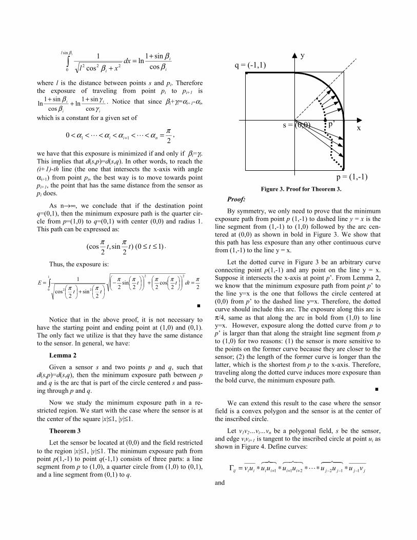
Theorem 3

Let the sensor be located at (0,0) and the field restricted to the region |x|≤1, |y|≤1. The minimum exposure path from point p(1,-1) to point q(-1,1) consists of three parts: a line segment from p to (1,0), a quarter circle from (1,0) to (0,1), and a line segment from (0,1) to q.

Proof:

By symmetry, we only need to prove that the minimum exposure path from point p (1,-1) to dashed line y = x is the line segment from (1,-1) to (1,0) followed by the arc cen-tered at (0,0) as shown in bold in Figure 3. We show that this path has less exposure than any other continuous curve from (1,-1) to the line y = x.

Let the dotted curve in Figure 3 be an arbitrary curve connecting point p(1,-1) and any point on the line y = x. Suppose it intersects the x-axis at point p’. From Lemma 2, we know that the minimum exposure path from point p’ to the line y=x is the one that follows the circle centered at (0,0) from p’ to the dashed line y=x. Therefore, the dotted curve should include this arc. The exposure along this arc is π/4, same as that along the arc in bold from (1,0) to line y=x. However, exposure along the dotted curve from p to p’ is larger than that along the straight line segment from p to (1,0) for two reasons: (1) the sensor is more sensitive to the points on the former curve because they are closer to the sensor; (2) the length of the former curve is longer than the latter, which is the shortest from p to the x-axis. Therefore, traveling along the dotted curve induces more exposure than the bold curve, the minimum exposure path.

� We can extend this result to the case where the sensor

field is a convex polygon and the sensor is at the center of the inscribed circle.

Let v1v2…vi…vn be a polygonal field, s be the sensor, and edge vivi+1 is tangent to the inscribed circle at point ui as shown in Figure 4. Define curves:

jjjjiiiiiiij vuuuuuuuuv 112211 −−−+++ ∗∗∗∗∗=ΓNUNQO

l

UQOUQO

and

q = (-1,1)

p = (1,-1)

s = (0,0) x

y

p’

Figure 3. Proof for Theorem 3.

jjjjiiiiiiij vuuuuuuuuv ∗∗∗∗∗=Γ +−−−−−

���

�

������

132211'

where iivu is the line segment from point ui to point vi,

�

1+iiuu is the arc on the inscribed circle between the two points that does not pass any other uj’s, * is the concatena-tion, and all +/– operations are modulus n. Notice that if vertices vi and vj are adjacent, one of these two curves be-comes edge jivv . We have:

Corollary 4

The minimum exposure path from vertices vi to vj is ei-ther Γij or Γ’ij whichever has less exposure.

Define the corner at a vertex vi as the area enclosed be

curve iiiiii vuuuuv 11 −− ∗∗���

, i.e., the region that is inside the polygon but outside the inscribed circle. From any point v in a corner other than the vertex vi, we draw two lines tangent to the circle: vv’ that intersects edge vi-1vi at v’ and is tangent to circle at u’; and vv” that intersects edge vivi+1 at v” and is tangent to circle at u”. Figure 5 shows this in a quadrilateral v1v2v3v4 and its inscribed circle centered at s. Consider point v in the corner at vertex v2. We want to find the minimum exposure path from v to a point in another corner, for exam-ple vertex v4, in the quadrilateral field. After drawing the two tangent lines vv’ and vv”, this problem is reduced to finding such a path in a smaller convex polygon v1v’vv”v3v4, which is solvable by Corollary 4. So we have:

Corollary 5

We can determine the minimum exposure path from one corner to another in a convex polygon.

However, the problem of finding the minimum expo-sure path between two points belonging to the same corner or when both are inside the inscribed circle (unless they are equidistant to the sensor) remains open.

V. GENERIC APPROACH FOR CALCULATING MINIMAL EXPOSURE PATH

As shown in Section IV, it is possible to obtain analyti-cal solutions to several simple instances of the exposure problem. However, finding the minimum exposure path in sensor networks under arbitrary sensor and intensity models is an extremely difficult optimization task. In this section we present a generic algorithm and several heuristics that can be used to obtain the solution to the exposure based cover-age problem.

The generic exposure problem domain is continuous and the exposure expression often does not have an analyti-cal solution. To address these characteristics, the algorithm we propose here has three main parts:

1) Transform the continuous problem domain to a dis-crete one;

2) Apply graph-theoretic abstraction;

3) Compute the minimal exposure path using Djikstra’s Single-Source-Shortest-Path algorithm [Cor90].

To transform the problem domain to a tractable discrete domain we use a generalized grid approach. For the sake of clarity, we restrict our subsequent discussion to the 2D case.

In the generalized grid-based approach, we divide the sensor network region using an nxn square grid and limit the existence of the minimal exposure path within each grid element. In the simplest case, the path is forced to exist only along the edges and the diagonals of each grid square as shown in Figure 6(a). We call this case the first-order grid. However, since the minimal exposure path can travel in arbitrary directions through the sensor field, it is easy to see that the first-order grid creates significant inaccuracies in the final results since it only allows horizontal, vertical, and diagonal movements. We use higher order grid structures such as the second-order and third-order grids shown in

u4

u3

u2u''

u1

s

v''

v2

v1 v4

u'

v'

v v3

Figure 5.

un

u4

uiu2

u1

s

vi

v2

v1 vn

Figure 4.

Figure 6(b) and 6(c) to improve the accuracy of the final solution. As can be deduced from Figure 6, to construct the m-th-order grid, we place m+1 equally spaced vertices along each edge of a grid square. The minimal exposure path is then restricted to straight line segments connecting any two of the vertices on each square. It is easy to verify that as n→∞ and m→∞, the solutions produced by the algo-rithm approaches the optimum, at the cost of run-time and storage requirements.

The details of the algorithm are listed in Figure 7. After generating the grid FD, the next step in the algorithm is to transform FD to the edge-weighted graph G. This is accom-plished by adding a vertex in G corresponding to each ver-tex in FD and an edge corresponding to each line segment in FD. Each edge is assigned a weight equal to the exposure along its corresponding edge in FD, calculated or approxi-mated by the Exposure() function. This function calculates the exposure along the line segment using numerical inte-gration techniques and can be implemented in a variety of ways.

As the pseudo-code in Figure 7 shows, we use Djik-stra’s Single-Source-Shortest-Path algorithm to find the minimal exposure path in G from the given source pS to the given destination pD. This algorithm can be replaced by the Floyd-Warshal All-Pair-Shortest-Path algorithm to find the minimal exposure path between any arbitrary starting and ending points on the grid FD. These two algorithms are well known and [Cor90] provides a detailed discussion on both.

When the starting and ending points of the path are ini-tially known, the run-time of the algorithm is generally dominated by the grid generation process which has a linear run time over |FD|, the total number of vertices in the grid. However, if the Single-Source-Shortest-Path algorithm is replaced by the All-Pair-Shortest-Path algorithm, then the run-time of the entire process is dominated by the shortest path calculation which has a complexity of O(|FD|3).

Procedure Minimal_Exposure_Path(F,pS,pD) { FD(V,L)=Generate_Grid(F,n,m) Init Graph G(V,E) For All vi∈ FD Add vertex vi’ to G For All li(vj,vk)∈ L Add edge ei(vj’,vk’) to G ei.weight=Exposure(li) vs = find closest vertex to pS ve = find closest vertex to pD Min_Exposure_Path=Single_Source_Shortest_Path(G, vs, ve) } Figure 7. Pseudo code for finding the minimal exposure path in

a sensor field F, given starting point pS and ending point pD.

VI. EXPERIMENTAL RESULTS In order to gain a deeper understanding of the exposure-

based model of coverage in sensor networks, we have per-formed a wide range of simulations and case-studies. In this section, we present several interesting results and discuss their implications and possible applications.

A. Simulation Platform The main simulation platform consists of a standalone

C++ package. The visualization and user interface elements are currently implemented using Visual C++ and OpenGL libraries. Network Simulator (NS) and a limited number of Rockwell seismic sensor nodes are also used to verify the sensing models and the qualitative performance of the expo-sure model in a realistic environment.

The sensor field in all experiments is defined as a square, 1000 meters wide. We have assumed a constant speed (|dp(t)/dt|=1) in all calculations of the minimal expo-sure path unless stated otherwise. This assumption signifi-cantly simplifies the required computation and allows for more visually intuitive results that are essential for demon-

Figure 6. First-order (a), second-order (b), and third-order (c) generalized 2x2 grid examples.

(a) n=2, m=1 (b) n=2, m=2 (c) n=2, m=3

stration purposes. The grid resolution in all cases is also fixed and was experimentally determined. In most cases, a 32x32 grid with 8 divisions per grid-square edge (n=32, m=8) were sufficient in producing accurate results.

B. Uniformly Distributed Random Sensor Deployment To create random sensor placements, we use two uni-

form random variables X and Y to compute the coordinates (xi,yi) of each sensor si in the field. The results in Table 1 and Table 2 show the mean, median, and standard deviation (µ) of exposure and path length calculated for 50 such cases. Table 1 lists results for varying number of sensors using the 1/d2 (K=2) model and Table 2 lists the results for the 1/d4 (K=4) sensing model. Both tables include results for the IA and IC intensity models.

As Tables 1 and 2 show, generally for sparse fields, there are a wide range of minimal exposure paths that can be expected from uniform random deployments. As sensor density increases in the field, the minimal exposure value and path lengths tend to stabilize. This effect can be ob-

served in Figure 9 that shows the relative standard deviation of exposure as the number of sensors increases. The results suggest that there is a saturation point after which randomly placing more sensors does not significantly impact the minimal exposure in the field. In our experiments we have observed that under the IA intensity model, as the number of sensors increase, the minimal exposure path generally gets closer to the bounding edges of the filed, and the path length approaches the half field perimeter value. This behavior is caused by the fact that sensors are only allowed to exist in the field and thus the boundary edges of the field are gener-ally farther from the bulk of sensors.

Figure 10 and Figure 11 show an instance of the mini-mal exposure path problem using the multi-resolution gen-eralized grid. Shown are the solutions obtained for a low resolution 8x8 grid, a higher resolution 16x16 grid, and an ultra-high resolution 32x32 grid under the IA and IC intensity models. It is interesting to note that using the very low-resolution 8x8 grid, the calculated path is fairly close to the accurate paths obtained by the higher resolution grids.

K=2 Intensity Model: All Sensors (IA) Intensity Model: Closest Sensor (IC) Exposure Path Length (m) Exposure Path Length(m)

Sensors Avg. Med. µµµµ

Avg. Med. µµµµ

Avg. Med. µµµµ

Avg. Med. µµµµ

23 0.29371 0.29364 0.043 1507.3 1537.9 258.3 0.07707 0.07386 0.023 1663.9 1671.9 205.7 26 0.33856 0.33542 0.051 1527.2 1538.0 269.0 0.08292 0.08200 0.024 1666.2 1673.5 214.4 27 0.35388 0.35310 0.054 1537.2 1607.1 280.7 0.08795 0.08490 0.023 1667.5 1688.2 228.5 74 1.21923 1.19378 0.133 1564.8 1576.2 229.2 0.22516 0.21827 0.049 1727.3 1757.3 169.8 79 1.29571 1.30208 0.130 1574.9 1558.9 245.8 0.23659 0.23168 0.046 1714.1 1700.0 183.3 85 1.43679 1.44794 0.127 1567.9 1568.1 203.4 0.25508 0.24577 0.049 1692.8 1689.8 181.8

119 2.18092 2.16669 0.147 1542.5 1552.7 233.2 0.35227 0.35154 0.056 1712.1 1707.6 155.2 126 2.32193 2.34368 0.176 1570.4 1577.5 209.3 0.36934 0.36404 0.059 1732.1 1702.4 151.8 146 2.78671 2.78598 0.202 1578.9 1595.3 196.1 0.42370 0.43267 0.059 1708.0 1714.1 121.6

Table 1. Uniformly distributed random sensor deployment statistics for 50 instances using 1/d2 sensing model.

K=4 Intensity Model: All Sensors (IA) Intensity Model: Closest Sensor (IC) Exposure (x10-5) Path Length (m) Exposure (x10-5) Path Length (m)

Sensors Avg. Med. µµµµ

Avg. Med. µµµµ

Avg. Med. µµµµ

Avg. Med. µµµµ

23 1.41637 0.95749 1.781 1617.6 1648.4 298.3 0.90822 0.43206 1.686 1753.4 1727.3 292.126 1.58834 1.10111 1.803 1718.7 1678.3 325.1 0.94988 0.51095 1.711 1807.6 1753.2 323.427 1.66767 1.19165 1.781 1678.6 1702.0 324.8 1.02837 0.61186 1.728 1726.9 1721.2 278.074 11.1643 8.99673 7.072 1777.1 1807.4 245.2 5.62326 3.79916 5.542 1881.0 1888.0 236.279 12.3447 10.3248 7.488 1730.7 1724.0 232.4 5.85618 4.19891 5.471 1833.4 1832.7 247.485 13.8395 11.9162 7.539 1696.0 1670.8 228.3 6.61165 4.96789 5.621 1838.0 1795.6 251.7

119 26.5454 23.3566 9.838 1783.6 1782.6 223.7 11.9136 9.45342 6.437 1872.5 1875.0 240.0126 28.6042 26.7352 10.186 1776.0 1783.2 210.5 12.5021 10.9340 6.468 1902.7 1883.2 217.0146 36.9259 34.6413 10.793 1755.4 1743.6 183.2 15.8885 14.0267 7.213 1861.8 1829.9 193.6

Table 2. Uniformly distributed random sensor deployment statistics for 50 instances using 1/d4 sensing model.

C. Deterministic Sensor Placement In addition to random deployments, we have studied the

effects of several regular, deterministic sensor placement strategies on exposure. Table 3 lists the exposure and path lengths for several such strategies of sensor deployment

using the 1/d2 (K=2) and 1/d4 (K=4) sensing models, IA and IC intensity models, and varying number of sensors.

In the cross deployment scheme, sensors are equally spaced along the horizontal and vertical line that split the square field in half. In the square-based approach, sensors

Figure 10. Minimum exposure path for 50 randomly deployed sensors under the All-Sensor intensity model (IA) and vary-ing grid resolutions: n=8, m=1 (left); n=16, m=2 (middle); n=32, m=8 (right).

Figure 11. Minimum exposure path for 50 randomly deployed sensors under the Closest-Sensor intensity model (IC) and varying grid resolutions: n=8, m=1 (left); n=16, m=2 (middle); n=32, m=8 (right).

20 52 84 116 1480.05

0.1

0.15

0.2

0.25

0.3

Number of Sensors

Rel

ativ

e St

d. D

ev.

20 52 84 116 1480.2

0.4

0.6

0.8

1.0

1.2

1.4

1.6

1.8

2 Exposure(K=4 Sensing Model)

Number of Sensors

Rel

ativ

e St

d. D

ev.

Exposure(K=2 Sensing Model)

IA

IC

IA

IC

Figure 9. Diminishing relative standard deviation in exposure for 1/d2 and 1/d4 sensor models.

are placed at the vertices of a grid. In the triangle- and hexagon-based methods, sensors are placed at the vertices of equally spaced triangular and hexagonal partitions in the sensor field. Clearly, numerous other placements can be constructed, however, these four cases serve as a guide on how coverage in deterministic deployment scenarios can differ from random cases.

In our experiments the cross-based deployment scheme seemed to provide the best level of exposure followed by the triangle-based scheme. The hexagon- and square-based schemes also present several interesting characteristics. Figure 12 and Figure 13 depict the deterministic deployment instances in action. Overall, the exposure along the minimal exposure path for the cross-, triangle-, square-, and hexa-gon-based deployment schemes was higher than the average randomly generated network topology. Finding the optimal placements of sensors to guarantee exposure coverage levels is an interesting and challenging problem. For example, in certain instances it may be desirable to detect objects enter-ing the field as soon as possible which may suggest placing sensors at the boundaries of the field. In other instances, more uniform coverage levels may be beneficial, suggesting the use of more uniform sensor deployment schemes such as the triangular and hexagonal deployment schemes.

VII. CONCLUSION Calculation of exposure is one of fundamental problem

in wireless ad-hoc sensor networks. We introduced the ex-posure-based coverage model, formally defined exposure, and studied several of its properties. Using a multiresolution technique and Dijkstra and/or Floyd-Warshall shortest path algorithms, we presented an efficient and effective algo-rithm for minimal exposure paths for any given distribution and characteristics of sensor networks. The algorithm works for arbitrary sensing and intensity models and provides an unbounded level of accuracy as a function of run time. The experimental results indicate that the algorithm can produce high quality results efficiently and can be used as a per-formance and worst-case coverage analysis tool in sensor networks.

This material is based upon work supported by DARPA and Air Force Research Laboratory under Contract No. F30602-99-C-0128. Any opinions, findings, conclusions, or recommendations expressed in this material are those of the authors’ and do not necessarily reflect the views of the DARPA and Air Force Re-search Laboratory.

Figure 12. Minimum exposure path under the All-Sensor intensity model (IA) using cross, square, triangle, and hexagon based deterministic sensor deployment schemes.

Figure 13. Minimum exposure path under the Closest-Sensor intensity model (IC) using cross, square, triangle, and hexagon based deterministic sensor deployment schemes.

VIII. REFERENCES [Abe00] H. Abelson, et. al. “Amorphous Computing.” Communications of

the ACM, vol. 43, (no. 5), pp. 74-82, May. 2000. [Abi00] A. A. Abidi, G.J. Pottie, W.J. Kaiser, “Power-Conscious Design

Of Wireless Circuits And Systems.” Proceedings of the IEEE, vol. 88, (no. 10), pp. 1528-45, Oct. 2000.

[Adj99] W. Adjie-Winoto, E. Schwartz, H. Balakrishnan, J. Lilley, “The Design And Implementation Of An Intentional Naming System.” Operating Systems Review, vol. 33, (no. 5), pp. 186-201, Dec. 1999.

[Bal98] H. Baltes, O. Paul, O. Brand, “Micromachined Thermally Based CMOS Micro-Sensors.” Proceedings of the IEEE, vol. 86, (no. 8), pp. 1660-78, Aug. 1998.

[Bra99] M.S. Braasch, A.J. Van Dierendonck, “GPS Receiver Architectures And Measurements.” Proceedings of the IEEE, vol. 87, (no. 1), pp. 48-64, Jan. 1999.

[Caf98] J. Caffery Jr., G.L. Stuber, “Subscriber Location In CDMA Cellular Networks.” IEEE Transactions on Vehicular Technology, vol. 47, (no. 2), pp. 406-16, May 1998.

[Caf00] J. Caffery Jr, G.L. Stuber, “Nonlinear Multiuser Parameter Estimation And Tracking In CDMA Systems.” IEEE Transactions on Communications, vol. 48, (no. 12), pp. 2053-63, Dec. 2000.

[Cor90] T. Cormen, C. Leiserson, R. Rivest, Introduction to Algorithms. MIT Pres, June 1990.

[Est00] D. Estrin, R. Govindan, J. Heidemann, “Embedding The Internet: Introduction.” Communications of the ACM, vol. 43, pp. 38-42, May. 2000.

[Fis99] S. Fisher, K. Ghassemi, “GPS IIF-The Next Generation.” Proceedings of the IEEE, vol. 87, (no.1), pp. 24-47, Jan. 1999.

[Gib96] J. D. Gibson, editor-in-chief, The mobile communications handbook. Boca Raton, CRC Press, New York, IEEE Press, 1996.

[Gre98] W. Gregg, W. Esaias, G. Feldman, R. Frouin, S. Hooker, C. McClain, R. Woodward, “Coverage Opportunities For Global Ocean Color In A Multimission Era.” IEEE Transactions on Geoscience and Remote Sensing, vol. 36, pp. 1620-7, Sept. 1998.

[Haa00] J. Haartsen, S. Mattisson, “Bluetooth - A New Low-Power Radio Interface Providing Short-Range Connectivity.” Proceedings of the IEEE, vol. 88, (no. 10), pp. 1651-61, Oct. 2000.

[Has97] Z. Haas, “On The Relaying Capability Of The Reconfigurable Wireless Networks.” IEEE 47th Vehicular Technology Conference, vol. 2, pp. 1148-52, May 1997.

[Kan00] C. Kang, M. Golay, “An Integrated Method For Comprehensive Sensor Network Developement In Complex Power Plant Systems.” Reliability Engineering & System Safety, vol. 67, pp. 17-27, Jan. 2000.

[Kou01] F. Koushanfar, et al. “Global Error-Tolerant Fault-Tolerant Algorithms for Location Discovery in Ad-hoc Wireless Networks.” UCLA Technical Report, UCLA Computer Science Department, 2001.

[Lan00] J. Lansford, P. Bahl, “The Design And Implementation Of HomeRF: A Radio Frequency Wireless Networking Standard For The

Sensor Model K=2 K=4 Intensity Model IA IC IA IC

Sensors Exp. Len. (m) Exp. Len. (m) Exp. (x10-5) Len. (m) Exp. (x10-5) Len. (m) Cross (+) 23 0.37921 1824.0 0.10534 1454.4 5.16387 1618.1 2.41489 1662.5 Cross (+) 79 1.81619 1885.5 0.46292 1626.3 263.737 1620.9 138.652 1659.8 Cross (+) 119 2.92691 1881.1 0.76240 1614.8 1076.93 1620.9 604.345 1655.5 Square 23 0.29164 1471.5 0.08075 1692.9 0.95149 1594.0 0.41017 1771.3 Square 79 1.53523 1452.6 0.35159 1688.5 17.3337 1613.2 7.40201 1835.4 Square 119 2.58348 1451.4 0.55955 1687.7 42.8954 1618.3 18.2303 1901.7 Triangle 27 0.41380 1730.6 0.12998 1713.3 1.92757 1785.3 1.04335 1783.4 Triangle 85 1.73666 1890.8 0.43943 1711.7 22.5250 2081.2 11.6667 1757.5 Triangle 126 2.78817 1917.6 0.65938 1708.4 51.3402 2010.2 26.2746 1775.7 Hexagon 26 0.38024 1455.1 0.10515 1630.0 1.58610 1559.2 0.67755 1845.1 Hexagon 74 1.48514 1450.9 0.34277 1642.2 16.6052 1776.4 7.03031 1864.1 Hexagon 146 3.43761 1446.9 0.70736 1624.3 72.4104 1545.5 31.3033 1795.1

Table 3. Deterministic sensor deployment results for several placement strategies. Location Error 1% 5% Intensity Model IA IC IA IC

Sensors Exp. Len. (m) Exp. Len. (m) Exp. Len. (m) Exp. Len. (m) 30 1.64 0.17 4.20 0.81 8.02 1.44 16.79 1.73 70 1.51 0.20 4.88 1.14 3.57 7.91 12.15 2.89

140 1.04 0.35 3.91 1.08 4.72 2.12 12.15 3.22 240 0.98 0.42 1.87 3.13 5.04 6.29 8.59 4.82 Table 4. Average exposure and path length errors due to uniform sensor location errors of 1% and 5% (K=2).

Connected Home.” Proceedings of the IEEE, vol. 88, (no. 10), pp. 1662-76, Oct. 2000.

[Lie98] K. Lieska, E. Laitinen, J. Lahteenmaki, “Radio Coverage Optimization With Genetic Algorithms.” IEEE International Symposium on Personal, Indoor and Mobile Radio Communications, vol. 1, pp. 318-22, Sept. 1998.

[Mar90] K. Marzullo, “Tolerating Failures Of Continuous-Valued Sensors.” ACM Transactions on Computer Systems, vol. 8, (no. 4), pp. 284-304, Nov. 1990.

[Mar96] M. Marengoni, B. Draper, A. Hanson, R. Sitaraman, “System To Place Observers On A Polyhedral Terrain In Polynomial Time.” Image and Vision Computing, vol. 18, pp. 773-80, Dec. 1996.

[Mas98] A. Mason, et al., “A Generic Multielement Microsystem For Portable Wireless Applications.” Proceedings of the IEEE, vol. 86, (no. 8), pp. 1733-46, Aug. 1998.

[Meg01] S. Meguerdichian, F. Koushanfar, M. Potkonjak, M. Srivastava, “Coverage Problems in Wireless Add-Hoc Sensor Networks.” Proceedings of IEEE Infocom, vol. 3, pp. 1380-1387, April 2001.

[Mol99] A. Molina, G.E. Athanasiadou, A.R. Nix, “The Automatic Location Of Base-Stations For Optimised Cellular Coverage: A New Combinatorial Approach.” IEEE 49th Vehicular Technology Conference, vol. 1, pp. 606-10, May 1999.

[Ngu98] C. Nguyen, L. Katehi, G. Rebeiz, “Micromachined Devices For Wireless Communications.” Proceedings of the IEEE, vol. 86, (no. 8), pp. 1756-68, Aug. 1998.

[Pri00] N. B. Priyantha, A. Chakraborty, H. Balakrishnan, “The Cricket Location-Support System.” Proceedings of the Sixth Annual ACM International Conference on Mobile Computing and Networking, pp. 32-43, August 2000.

[Pot00] G. J. Pottie, W. J. Kaiser, “Wireless Integrated Network Sensors.” Communications of the ACM, vol. 43, (no. 5), pp. 51-58, May. 2000.

[Rit77] S. Riter, J. MacCoy. “Automatic Vehicle Locaiton - An Overview.” IEEE transaction on vehicular technology, vol. VT26, no 1, Feb 1977.

[Sha99] M. Shaw, P. Levin, J. Martel, “The Dod: Stewards Of A Global Information Resource, The Navstar Global Positioning System.” Proceedings of the IEEE, vol. 87, (no. 1), pp. 16-23, Jan. 1999.

[Ten00] D. Tennenhouse, “Proactive computing.” Communications of the ACM, vol. 43, (no. 5), pp. 43-50, May. 2000.

[Tur72] G.L. Turin, W.S. Jewell, T.L. Johnston, “Simulation Of Urban Vehicle-Monitoring Systems.” IEEE Transactions on Vehicular Technology, vol. vt21, (no. 1), pp. 9-16, Feb. 1972.

[Wan92] R. Want, A. Hopper, “Active Badges And Personal Interactive Computing Objects.” IEEE Transactions on Consumer Electronics, vol. 38, (no. 1), pp. 10-20, Feb. 1992.

[Yaz00] N. Yazdi, A. Mason, K. Najafi, K. Wise, “A Generic Interface Chip For Capacitive Sensors In Low-Power Multi-Parameter Micro-Systems.” Sensors and Actuators A (Physical), vol. A84, (no. 3), pp. 351-61, Sept. 2000.