
Experimental Investigation of Ion Temperature … · Experimental Investigation of Ion Temperature...
135
Experimental Investigation of Ion Temperature Anisotropy Driven Instabilities in a High Beta Plasma Paul A. Keiter Dissertation submitted to the College of Arts and Sciences at West Virginia University in partial fulfillment of the requirements for the degree of Doctor of Philosophy in Plasma Physics Earl Scime, PhD., Chair Mark Koepke, PhD. Arthur Weldon, PhD. Richard Treat, PhD, Charter Stinespring, PhD. Department of Physics Morgantown, West Virginia 1999 Keywords: Ion Temperature Anisotropy, Helicon Source
Transcript of Experimental Investigation of Ion Temperature … · Experimental Investigation of Ion Temperature...

Experimental Investigation of Ion Temperature Anisotropy
Driven Instabilities in a High Beta Plasma
Paul A. Keiter
Dissertation submitted to the College of Arts and Sciences
at West Virginia University
in partial fulfillment of the requirements
for the degree of
Doctor of Philosophy
in
Plasma Physics
Earl Scime, PhD., Chair
Mark Koepke, PhD.
Arthur Weldon, PhD.
Richard Treat, PhD,
Charter Stinespring, PhD.
Department of Physics
Morgantown, West Virginia
1999
Keywords: Ion Temperature Anisotropy, Helicon Source

ii
1 ABSTRACT
The first measurements of an ion temperature anisotropy/beta inverse correlation in a
high beta laboratory experiment are presented. The observation of this correlation is
similar to such a correlation present in in-situ spacecraft measurements and predicted in
theory. Low-frequency fluctuations are also observed. According to measurements
presented here, these waves are electromagnetic, transverse, occur at frequencies below
the cyclotron frequency and have wavenumbers consistent with predictions for the ion
cyclotron anisotropy instability, also referred to as the Alfvén Ion-Cyclotron instability.
The device is a space simulation chamber that uses a helicon source for its plasma source.
Ranges of ion beta and ion temperature anisotropy are 10-4 to 10-2 and 1 to 15,
respectively. The correlation is experimentally determined to be 5.0|||| 15.01 −
⊥ += iTT β .

iii
2 ACKNOWLEDGEMENTS
I would like to thank my advisor, Professor Earl Scime for his support and guidance
throughout this project. I would also like to thank Professor Mark Koepke for helpful
discussions and for development of the laser system. I would like to thank the other
members of my committee, Professor Charter Stinespring, Professor Richard Treat and
Professor Arthur Weldon for their contributions. Thanks to Mike Zintl for his guidance
and assistance with the laser system. I would like to thank Doug Mathess, Tom Milan,
and Carl Weber for the construction of the experiment and probes. Thanks also go to
Matt Balkey and John Kline for their contributions to the development of the experiment
and helpful discussions. I would also like to thank my family for their constant support
throughout this work.
iv
1 Abstract................................................................................................................... ii 2 Acknowledgements ................................................................................................ iii 3 Introduction............................................................................................................. 1 4 Plasma Experiment.................................................................................................. 4
4.1 Plasma Source ..................................................................................................... 6 4.2 Helicon Sources................................................................................................. 16
4.2.1 Background ............................................................................................... 16 4.2.2 Helicon Dispersion Relation ...................................................................... 22 4.2.3 Possible Explanations of Efficient Ionization in Helicon sources................ 28
4.3 Space Simulation Chamber................................................................................ 33 4.4 Data Acquisition System ................................................................................... 35
5 Diagnostics............................................................................................................ 37 5.1 Langmuir Probe................................................................................................. 37
5.1.1 Determination of electron density and temperature..................................... 39 5.1.2 Langmuir Probe Design ............................................................................. 40
5.2 Laser Induced Fluorescence............................................................................... 44 5.2.1 Line Broadening Mechanisms.................................................................... 49
5.2.1.1 Natural Linewidth .................................................................................. 49 5.2.1.2 Doppler Broadening............................................................................... 50 5.2.1.3 Pressure Broadening .............................................................................. 51 5.2.1.4 Zeeman Broadening ............................................................................... 52 5.2.1.5 Power Broadening.................................................................................. 53 5.2.1.6 Instrumental Broadening ........................................................................ 54 5.2.1.7 Comparison of Broadening Mechanisms ................................................ 54
5.3 Magnetic Probe ................................................................................................. 57 5.3.1 Magnetic probe construction and calibration .............................................. 57 5.3.2 Analysis of magnetic probe signals ............................................................ 63
6 Electromagnetic Ion Temperature Anisotropy Driven Instabilities ......................... 68 6.1 Linear Vlasov Solution ...................................................................................... 69 6.2 Recent Spacecraft Observations......................................................................... 78 6.3 Previous Experimental Investigations of EMITA Instabilities ............................ 84
7 Experimental Results on Ion Temperature Anisotropy Upper Bound ..................... 86 7.1 Inverse Correlations of ||ii TT ⊥ and ||iβ .............................................................. 86
7.2 Collisions .......................................................................................................... 91 7.3 Anisotropy Reduction by waves ........................................................................ 97
8 Identification of the waves................................................................................... 102 8.1 Wave Power Spectra and Amplitude Measurements ........................................ 102 8.2 Wavenumber Measurements............................................................................ 112
9 Discussion ........................................................................................................... 125 10 References........................................................................................................... 127

1
3 INTRODUCTION
The results presented in this thesis are from the first high-beta ( 28 BnkTπβ = ),
steady-state laboratory experiment to verify the ion temperature anisotropy/beta inverse
correlation observed by spacecraft in the magnetosphere. Manheimer and Boris1 first
proposed the idea that a plasma instability threshold derived from linear theory should
correspond to an observable bound on the anisotropy driving the unstable mode.
Computational simulations2, 3 of magnetospherically relevant plasmas have been used to
interpret the ion temperature anisotropy/beta inverse correlation observed by spacecraft
as an upper bound on the ion temperature anisotropy in the magnetosphere.4, 5, 6 If this
interpretation were correct, it would support the Manheimer and Boris idea. Previous
laboratory experiments have observed electromagnetic ion temperature anisotropy driven
instabilities.7, 8, 9 However, none have reported observations of an ion temperature
anisotropy/beta inverse correlation. Here, measurements clearly show this inverse
correlation and that the reduction of the ion temperature anisotropy is correlated with the
amplitude of low frequency ( ciωω ≤≤5.0 ), electromagnetic fluctuations. Measured
characteristics of these fluctuations are consistent with those of the ion cyclotron
anisotropy instability, also known as the Alfvén ion cyclotron instability. The scaling of
the upper bound on the ion temperature anisotropy with plasma beta is also in good
agreement with spacecraft observations in the magnetosheath.
The wide range of plasma regimes in the near-Earth space environment provides
unparalleled opportunities for testing the predictions of theory and computation.
Unfortunately, in space, controlled experiments are rarely possible. Single-point
spacecraft observations have provided a wealth of information concerning a variety of
instabilities. This information has been used to test existing theories and lay the
groundwork for new theories. However, single-point spacecraft measurements cannot
perform reproducible experiments and cannot separate spatially varying from temporally
varying plasma phenomena. From a moving spacecraft, a spatial variation appears as a
temporal variation. In addition, spacecraft cannot measure the wavelengths of instabilities

2
much larger than themselves. In order to obtain a wavelength measurement, time series
measurements must be measured at a minimum of two different spatial locations.
The Large Experiment on Instabilities and Anisotropies (LEIA) experiment at West
Virginia University (WVU) is designed to generate controlled levels of ion temperature
anisotropy to investigate ion temperature anisotropy driven instabilities in a fully
diagnosed laboratory experiment. Although other laboratory experiments have observed
ion temperature anisotropy driven instabilities, those experiments were not intended to
address issues relevant to magnetosheath simulations and in-situ space data. The results
presented here represent an effort to corroborate laboratory experimental results with
computational models and spacecraft observations.
A key element in the interpretation of spacecraft results has been the use of theory and
computational simulations. In the case of ion temperature anisotropy driven instabilities,
hybrid-kinetic simulations suggest that the inverse correlation between the plasma beta
and the ion temperature anisotropy in the magnetosheath arises from velocity space
diffusion due to ion cyclotron anisotropy instabilities. The frequencies of and the levels
of wave activity seen by the spacecraft are also consistent with the models.
The apparatus used for these experiments is described in Chapter 4. In addition to
descriptions of the hardware and the data acquisition system, background information
concerning helicon plasma sources and previous results are reviewed. The space
simulation chamber is also described in Chapter 4. In Chapter 5, the diagnostic tools used
in the space simulation chamber, including Langmuir probes, laser induced fluorescence
(LIF) probes, and magnetic probes are discussed.
A brief review of the theory of ion temperature anisotropy driven instabilities is
provided in Chapter 6. Although the observed values of ion temperature anisotropy in
LEIA ( )1|| >⊥ TT could permit both the ion cyclotron instability and the mirror instability
to exist, the value of ion beta in LEIA ( 1<β ) results in the dominance of the ion
cyclotron instability. Predictions of the beta-dependant ion temperature anisotropy upper
bound from computational models and in-situ spacecraft measurements of both ion
temperature anisotropy and wave measurements are also presented in Chapter 6.
Laboratory measurements of the ion temperature anisotropy upper bound are
presented and compared to theory and spacecraft observations in Chapter 7. The effects
3
of varying the collisionality and the role of low frequency waves reducing the ion
temperature anisotropy are also discussed in Chapter 7.
In Chapter 8, the predicted scaling of the amplitude and the characteristics of
magnetic fluctuations are compared to measurements in LEIA. In-situ magnetosheath
observations of the beta-dependant upper bound on the ion temperature anisotropy
without observations of strong wave activity present are reviewed and wavenumbers for
the experimental cases studied are also compared to theoretical predictions in Chapter 8.
The experimental results are summarized and possible directions for future work are
discussed in Chapter 9.

4
4 PLASMA EXPERIMENT
The apparatus used in these experiments was designed to provide an environment for
performing high beta, magnetospherically relevant plasma experiments. To achieve high
values of beta ( 01.0>β ), a high-density plasma confined by a low magnetic field is
desired. A high-density plasma was created in a helicon plasma source, HELIX (Hot
hELIcon eXperiment) (Figure 1), and allowed to expand into LEIA (Large Experiment
on Instabilities and Anisotropies), a space simulation chamber (Figure 2). LEIA is a low
magnetic field, large volume chamber. Typical ion β values for different plasma
environments are tabulated in Table 1. A value of 0.01 is considered high ion beta for the
purposes of the experiments described here. It is true that magnetosheath beta values
often exceed 10 to 100, but the intention of these experiments is to investigate specific
microphysical issues and not to reproduce the magnetosheath exactly.
Table 1: Typical ion beta values for various plasma environments.
Environment n (cm-3) Ti(eV) B (G) ββi
Magnetosheath10 8 150 1.5 x 10⁻⁴ ≥ 1
Heliosphere10 7 10 7 x 10⁻⁵ ~ 1
Tokamak (TFTR)11 1014 32,000 56,000 4 x 10⁻²
LEIA 1012 0.3 35 1 x 10⁻²
Tokamak 12
(Alcator C-MOD) 3 x 10¹⁴ 600 30,000 8 x 10⁻³
HELIX 1014 0.5 500 8 x 10⁻³
Ionosphere10 105 .2 .26 1 x 10⁻⁵
Q-machine13 1012 .2 1000 8 x 10⁻⁶

5
Figure 1: HELIX (foreground) and LEIA (large aluminum chamber). HELIX resides inside a Faraday cage (copper screening). The large electromagnets surrounding LEIA
are roughly 3 m in diameter.
Heating AntennaHelicon Source
ToPump
To
DownstreamLIF
UpstreamLIF
LEIA
Pump
4.4 m 1.6 m
Figure 2: Schematic of LEIA and HELIX.

6
Figure 3: The HELIX plasma source. On the right side is the mating flange to the pumping station. Sitting on the rails are ten electromagnets used to confine the plasma. The matching circuit and the antenna are to the lower right of the picture. At the top of
the picture, copper screening, which composes part of the Faraday cage, is visible.
4.1 Plasma Source
The helicon source (Figure 3) is a Pyrex tube, 157 cm long and 15 cm in diameter.
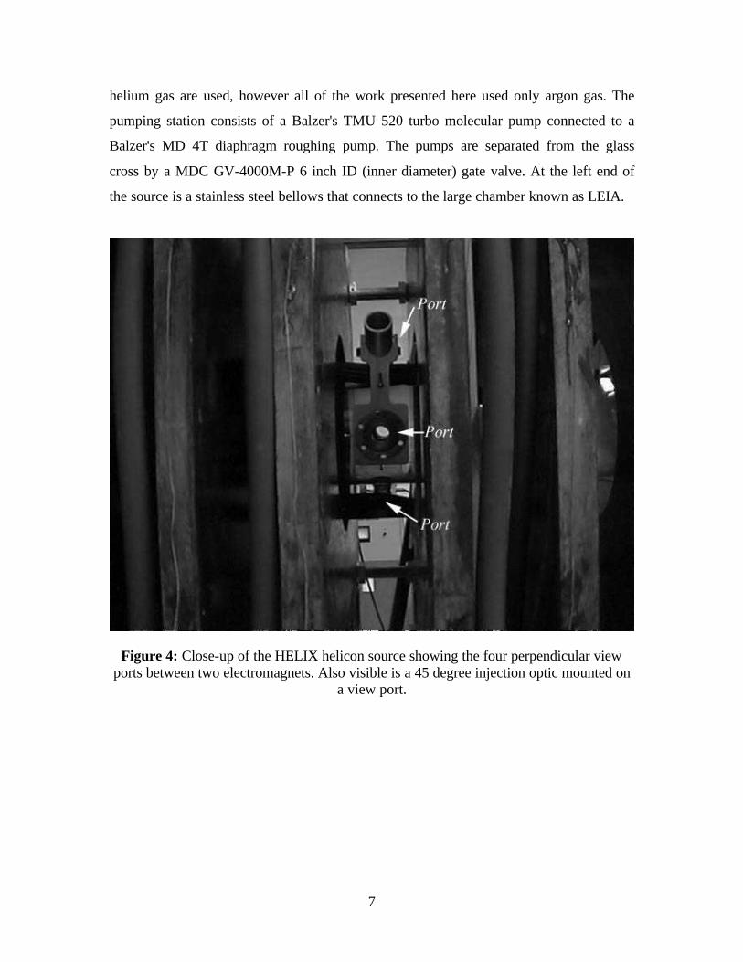
Typical operating parameters for HELIX are listed in Table 2. There are four
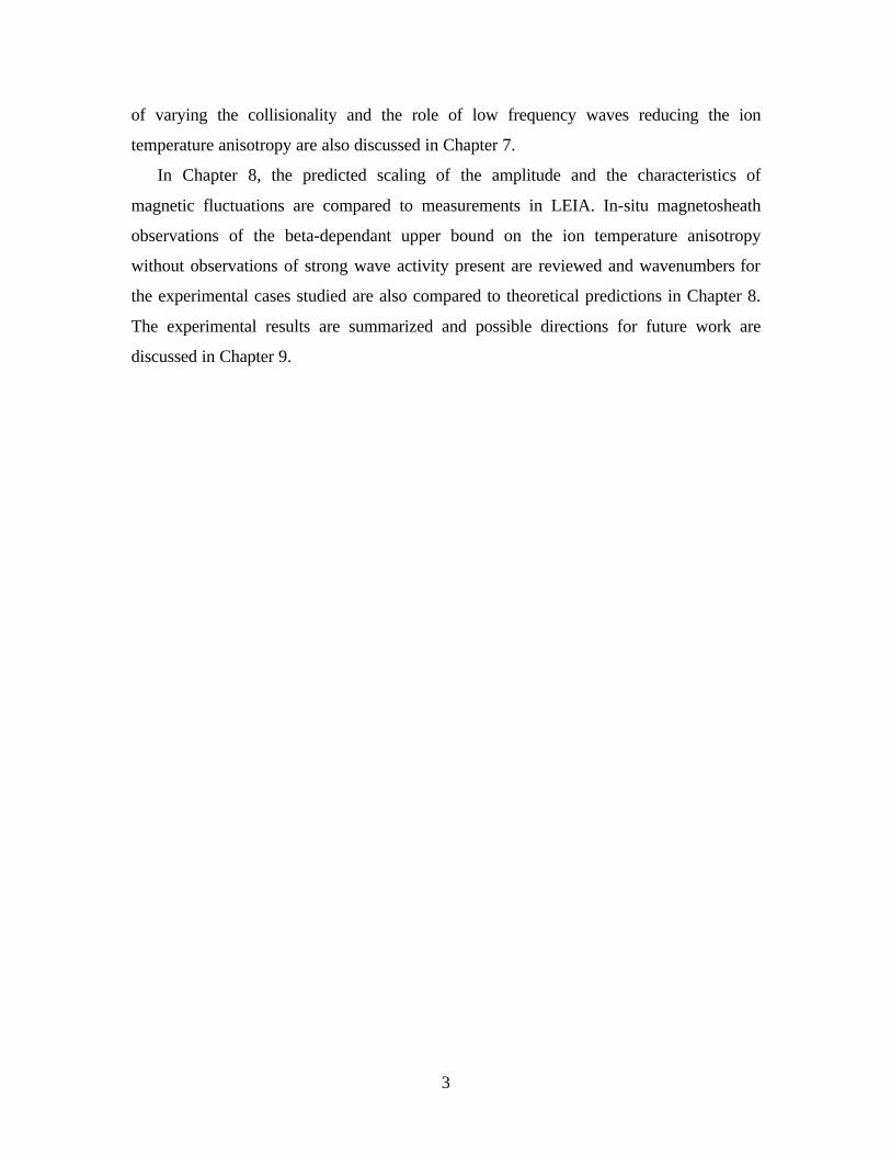
perpendicular view ports (see Figure 4) to allow optical access to the source. Copper
screening around the helicon source forms a Faraday cage. The Faraday cage prevents
extraneous high frequency electromagnetic signals from entering the source chamber and
prevents the rf driving signal from radiating into the laboratory. At the right-hand side of
Figure 3 is a stainless steel mating flange that connects the helicon source to the pumping
station. Gas is fed into the chamber through a valve in the mating flange. Both argon and
7
helium gas are used, however all of the work presented here used only argon gas. The
pumping station consists of a Balzer's TMU 520 turbo molecular pump connected to a
Balzer's MD 4T diaphragm roughing pump. The pumps are separated from the glass
cross by a MDC GV-4000M-P 6 inch ID (inner diameter) gate valve. At the left end of
the source is a stainless steel bellows that connects to the large chamber known as LEIA.
Figure 4: Close-up of the HELIX helicon source showing the four perpendicular view ports between two electromagnets. Also visible is a 45 degree injection optic mounted on
a view port.
8
Table 2: Standard operating parameters for HELIX
Parameter Typical HELIX Values
Gas Species Argon
Source Length 157 cm
Source Radius 15 cm
Base Pressure < 2 x 10 -8 Torr
Operating Pressure 1 - 10 mTorr
Magnetic Field < 1300 G
RF Power 0 - 500 W
Operating Frequency 7 - 15 MHz
Density ≤ 1014 cm-3
Electron Temperature ~5 eV
Ion Temperature < 1 eV
Ion Temperature Anisotropy ( )||TT⊥ 1 - 5
Electron Gyroradius ~ .03 mm
Ion Gyroradius ~ .12 mm
The magnetic field for the helicon source is created by ten electromagnets donated by
the Max Planck Institüt in Garching, Germany. The magnets have 46 internal copper
windings with a resistance of 17 mΩ and an inductance of 1.2 mH. The magnets are
water cooled to prevent overheating. The magnets roll on a pair of rails that allow their
axial positions to be adjusted. A Macroamp 300 A power supply provides the current for
the electromagnets. The magnetic field in HELIX can be varied from 0 to 1300 Gauss.
The on-axis magnetic field in HELIX is given by
IB 93.308.6 += , (1)
where I is the coil current. This relationship was determined experimentally by varying
the current supplied to the magnets and measuring the magnetic field with a gaussmeter.

9
Presently, the second magnet from the end of the source closest to the pumping station
has been reversed to create a field null. The field null was used to isolate the pumping
station from the plasma and because other helicon source groups have reported increased
densities using field nulls near one end of the helicon antenna. 14
200
300
400
500
600
700
800
0 20 40 60 80 100 120 140
Bz (
G)
Z (cm)
Figure 5: Magnetic field strength as a function of axial position (z) in HELIX.
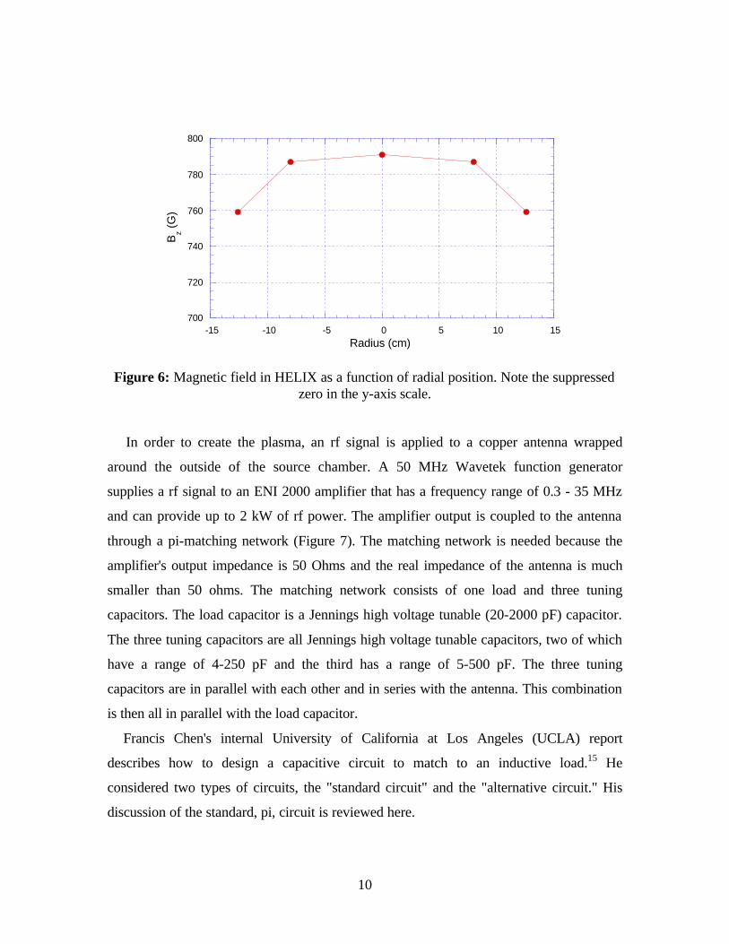
The azimuthal and radial zB magnetic field profiles in HELIX are shown in Figure 5 and
Figure 6. The radial magnetic field is uniform to within 1% over the chamber radius and
uniform to within 5% along the central meter of the chamber.
10
700
720
740
760
780
800
-15 -10 -5 0 5 10 15
Bz (
G)
Radius (cm)
Figure 6: Magnetic field in HELIX as a function of radial position. Note the suppressed zero in the y-axis scale.
In order to create the plasma, an rf signal is applied to a copper antenna wrapped
around the outside of the source chamber. A 50 MHz Wavetek function generator
supplies a rf signal to an ENI 2000 amplifier that has a frequency range of 0.3 - 35 MHz
and can provide up to 2 kW of rf power. The amplifier output is coupled to the antenna
through a pi-matching network (Figure 7). The matching network is needed because the
amplifier's output impedance is 50 Ohms and the real impedance of the antenna is much
smaller than 50 ohms. The matching network consists of one load and three tuning
capacitors. The load capacitor is a Jennings high voltage tunable (20-2000 pF) capacitor.
The three tuning capacitors are all Jennings high voltage tunable capacitors, two of which
have a range of 4-250 pF and the third has a range of 5-500 pF. The three tuning
capacitors are in parallel with each other and in series with the antenna. This combination
is then all in parallel with the load capacitor.
Francis Chen's internal University of California at Los Angeles (UCLA) report
describes how to design a capacitive circuit to match to an inductive load.15 He
considered two types of circuits, the "standard circuit" and the "alternative circuit." His
discussion of the standard, pi, circuit is reviewed here.

11
Figure 7: Schematic of the standard circuit. C1 is the load capacitor, C2 is the tuning capacitors and R+L comprise the real resistance and inductance of the antenna.
In Chen's analysis, all the impedances are normalized to Ro= 50 Ω. Thus, to maximize
the efficiency of the circuit, the circuit elements are chosen such that the real part of the
impedance is 1 and the imaginary part is 0. In terms of the impedance of the combined
load and matching circuit system, the input impedance (Z) is.
( ) 112
11
−−− += ZZZ (2)
where,
1
1 C
iZ
ω−= , and
22 C
iiXRZ
ω−+= . (3)
R is the real resistance of the antenna and X is the reactance of the antenna. 1C is the load
capacitor and 2C is the tuning capacitor. Substituting these expressions into equation (2),
( )
( )( )( )
( ) 21
2221
11
121
2
1
1
1
1
CRQC
RCiQCiQR
RCiCiXC
CXiRZ
ωωωω
ωωωω
+−−−+
=+−−
−+= , (4)
where
21 CXQ ω−≡ . (5)
Defining
( ) 21
22211 CRQCD ωω +−≡ , (6)
12
the impedance can be separated into real and imaginary parts and written as
( ) ( ) QRCQCRZD 111Re ωω +−= (7)
( ) ( ) 12
11Im CRQCQZD −−= ω (8)
which reduces to
( ) RZD =Re (9)
and
( ) ( )221Im QRCQZD +−= ω . (10)
Requiring ( ) 0Im =Z yields,
( )221 QRCQ += ω . (11)
Substituting this into equation (6):
.1 1QCD ω−= (12)
Setting ( ) 1Re =Z requires:
( ) 11 1 =− QCR ω (13)
and solving the quadratic for Q yields:
( ) QRC −= 1 1ω . (14)
Rewriting equation (11), Q can be written as a quadratic
021
21 =+− RCQQC ωω . (15)
Thus,
( ) 21
221
21 4112 RCQC ωω −±= . (16)
Combining equations (14) and (16),
( ) 21
221
24121 RCR ω−±=− . (17)
With this result it is possible to determine the load capacitance necessary to match the
circuit independent of the antenna reactance. Squaring both sides and solving for 1C
( ) 221
22 4121 RCR ω−=− (18)
( )[ ] RRC ω22112
12
1 −−= . (19)

13
Using this value for 1C , 2C can be determined as a function of 1C , R, ω, and X.
Combining equations (5) and (14) yields
1
12
1−
−−=
C
RXC
ωω . (20)
The solutions for 1C and 2C can be rewritten as
21
2
1
211
2
1
−−=
oR
R
RC
ω (21)
1
12
1−
−−=
C
RRXC oω . (22)
For a purely inductive load ( )LX ω= , such as is expected for the HELIX configuration,
( ) 121
2 1 CRRLC o−−=− ω . (23)
Solutions for 1C and 2C for a purely inductive load are graphed in Figure 8 and Figure 9
respectively. If ( ) 121 CRRL o ω−< , there is no positive solution for 2C . For the typical
case of 1<<oRR , equations (21) and (22) can be approximated by
( ) 21
1−≈ oRRCω and ( )[ ] 1
22
1 −−≈ oRRXCω . (24)
Figure 8: Relationship between the capacitance and inductance of the load capacitor in a matching circuit for 13.56 (top curve) and 27.12 (bottom curve) MHz as shown by
Chen.15
14
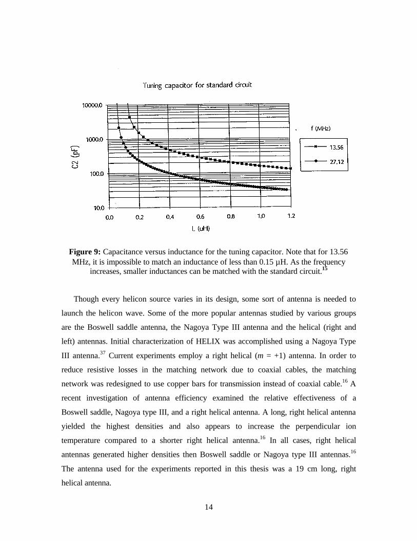
Figure 9: Capacitance versus inductance for the tuning capacitor. Note that for 13.56 MHz, it is impossible to match an inductance of less than 0.15 µH. As the frequency
increases, smaller inductances can be matched with the standard circuit.15
Though every helicon source varies in its design, some sort of antenna is needed to
launch the helicon wave. Some of the more popular antennas studied by various groups
are the Boswell saddle antenna, the Nagoya Type III antenna and the helical (right and
left) antennas. Initial characterization of HELIX was accomplished using a Nagoya Type
III antenna.37 Current experiments employ a right helical (m = +1) antenna. In order to
reduce resistive losses in the matching network due to coaxial cables, the matching
network was redesigned to use copper bars for transmission instead of coaxial cable.16 A
recent investigation of antenna efficiency examined the relative effectiveness of a
Boswell saddle, Nagoya type III, and a right helical antenna. A long, right helical antenna
yielded the highest densities and also appears to increase the perpendicular ion
temperature compared to a shorter right helical antenna.16 In all cases, right helical
antennas generated higher densities then Boswell saddle or Nagoya type III antennas.16
The antenna used for the experiments reported in this thesis was a 19 cm long, right
helical antenna.
15
HELIX is different from most helicon sources because it is operated steady-state.
Running steady-state allows for the same plasma environment to be studied during a
series of measurements. However, probes placed in the plasma degrade much faster than
in a pulsed source. This increases the level of contaminants in the system. To counteract
this, all measurements performed in HELIX use non-invasive techniques.
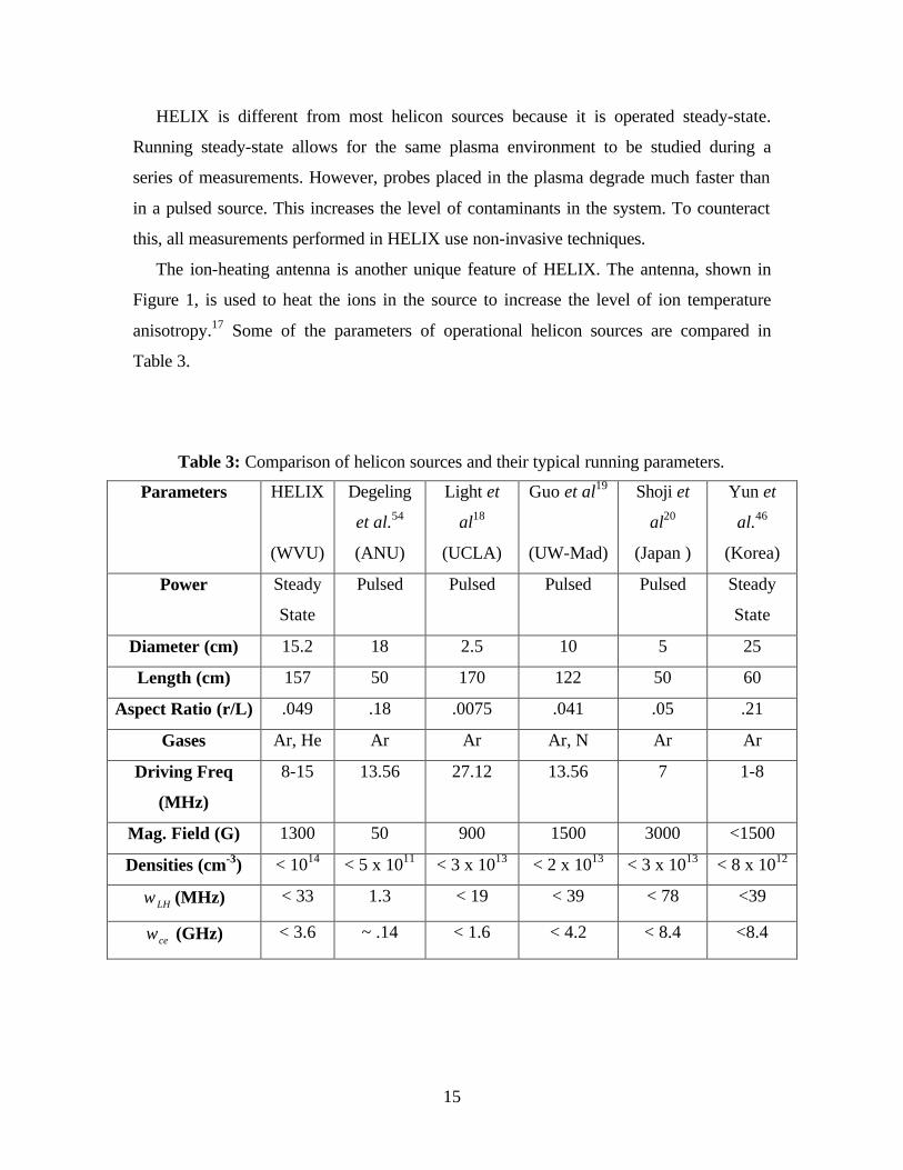
The ion-heating antenna is another unique feature of HELIX. The antenna, shown in
Figure 1, is used to heat the ions in the source to increase the level of ion temperature
anisotropy.17 Some of the parameters of operational helicon sources are compared in
Table 3.
Table 3: Comparison of helicon sources and their typical running parameters.
Parameters HELIX
(WVU)
Degeling
et al.54
(ANU)
Light et
al18
(UCLA)
Guo et al19
(UW-Mad)
Shoji et
al20
(Japan )
Yun et
al.46
(Korea)
Power Steady
State
Pulsed Pulsed Pulsed Pulsed Steady
State
Diameter (cm) 15.2 18 2.5 10 5 25
Length (cm) 157 50 170 122 50 60
Aspect Ratio (r/L) .049 .18 .0075 .041 .05 .21
Gases Ar, He Ar Ar Ar, N Ar Ar
Driving Freq
(MHz)
8-15 13.56 27.12 13.56 7 1-8
Mag. Field (G) 1300 50 900 1500 3000 <1500
Densities (cm-3) < 1014 < 5 x 10¹¹ < 3 x 10¹³ < 2 x 10¹³ < 3 x 10¹³ < 8 x 10¹²
LHω (MHz) < 33 1.3 < 19 < 39 < 78 <39
ceω (GHz) < 3.6 ~ .14 < 1.6 < 4.2 < 8.4 <8.4
16
4.2 Helicon Sources
The helicon plasma source is a high-density, highly efficient, inductively coupled
plasma source that was first described in 1970 by Boswell.21 The helicon plasma source
has been used as a source for materials processing,22, 23, 24, 25, 26 for magnetic fusion27
(Heliac), for high beta, space simulation experiments, and for space plasma thruster
development.28 Many groups have attempted to explain the mechanism for the efficient
ionization of helicon sources by Landau damping, energetic beams of electrons, and
Trivelpiece-Gould (TG) waves. At present, a definitive answer has not been obtained.
4.2.1 Background
The term "helicon" was first used by Aigrain29 in 1960 to describe an electromagnetic
wave propagating in a low temperature solid metal with a frequency between the ion and
electron cyclotron frequencies, i.e., a whistler wave. Around 1964, Legendy30 in the
United States and Klosenberg, McNamara and Thonemann31 in the United Kingdom
developed theories concerning the propagation of helicon waves in cylindrical
magnetoplasmas. In 1968, Boswell constructed a helicon experiment at Flinders
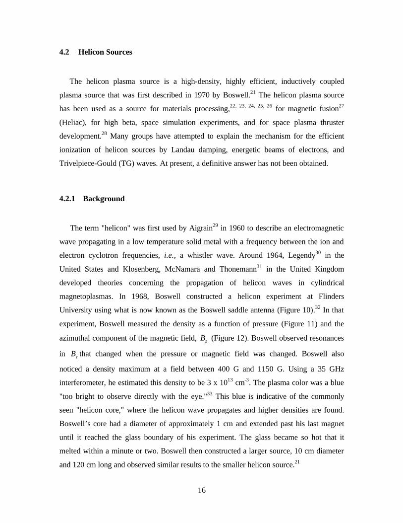
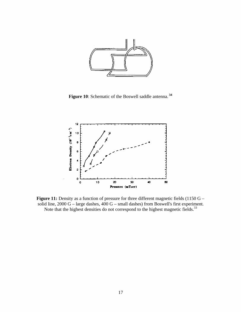
University using what is now known as the Boswell saddle antenna (Figure 10).32 In that
experiment, Boswell measured the density as a function of pressure (Figure 11) and the
azimuthal component of the magnetic field, zB (Figure 12). Boswell observed resonances
in zB that changed when the pressure or magnetic field was changed. Boswell also
noticed a density maximum at a field between 400 G and 1150 G. Using a 35 GHz
interferometer, he estimated this density to be 3 x 1013 cm-3. The plasma color was a blue
"too bright to observe directly with the eye."33 This blue is indicative of the commonly
seen "helicon core," where the helicon wave propagates and higher densities are found.
Boswell’s core had a diameter of approximately 1 cm and extended past his last magnet
until it reached the glass boundary of his experiment. The glass became so hot that it
melted within a minute or two. Boswell then constructed a larger source, 10 cm diameter
and 120 cm long and observed similar results to the smaller helicon source.21
17
Figure 10: Schematic of the Boswell saddle antenna. 34
Figure 11: Density as a function of pressure for three different magnetic fields (1150 G – solid line, 2000 G – large dashes, 400 G – small dashes) from Boswell's first experiment.
Note that the highest densities do not correspond to the highest magnetic fields.33

18
Figure 12: Measured zB for 9 mTorr (solid line) and 27 mTorr (dashed line). Resonances
in zB appear to change with different pressures.33
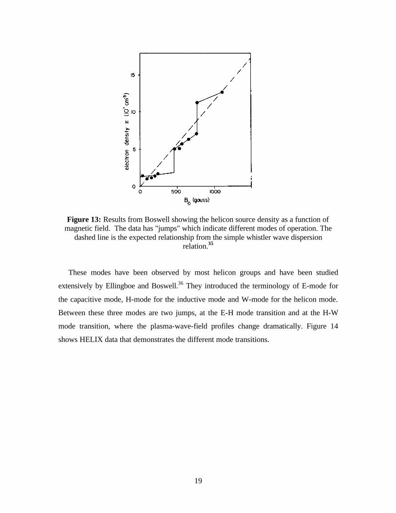
Boswell was one of the first researchers to report “jumps” in the helicon source
density.35 Physically, these jumps correspond to an increase in plasma brightness
(density). Figure 13 shows Boswell's measurements of the electron density versus
magnetic field in an early helicon source. Even though the general trend of the data is
well fit with a straight line corresponding to the whistler dispersion relationship, the
plasma density is roughly constant across small ranges of magnetic field. Between the
constant density regions, there is a sudden transition to another density value as the
magnetic field is increased. These jumps occur when there is a mode transition in the
helicon source. Three modes of operation have been identified, the capacitive, the
inductive and the helicon mode.
19
Figure 13: Results from Boswell showing the helicon source density as a function of magnetic field. The data has "jumps" which indicate different modes of operation. The
dashed line is the expected relationship from the simple whistler wave dispersion relation.35
These modes have been observed by most helicon groups and have been studied
extensively by Ellingboe and Boswell.36 They introduced the terminology of E-mode for
the capacitive mode, H-mode for the inductive mode and W-mode for the helicon mode.
Between these three modes are two jumps, at the E-H mode transition and at the H-W
mode transition, where the plasma-wave-field profiles change dramatically. Figure 14
shows HELIX data that demonstrates the different mode transitions.

20
1010
1011
1012
1013
0.0 0.5 1.0 1.5 2.0
1000 G800 G600 G500 G400 G200 G
Power (kW)
Figure 14: Density as a function of rf power for six different magnetic fields from HELIX. 37 Note the jumps in density, which represent different modes of operation.
The E-H transition in HELIX occurs at a density of roughly 1011 cm-3 regardless of the
magnetic field or pressure. This transition is related to the electron skin depth, pec ωδ = ,
where ( ) 2124 eepe menπω = is the electron plasma frequency. The E-H transition generally
occurs when δ is approximately half the chamber diameter.
There is a well-documented change in the density profile at the H-W transition. In the
H mode, the profiles are often observed to be hollow, while the profiles are much more
centrally peaked in the W mode. Traveling waves become observable in the W mode, as
opposed to the standing waves associated with the E and H modes. As shown in Figure
14, the H mode often exists over a very small range of parameters and can often go
unnoticed. Recently, the helicon community has shifted its focus from discussion of the
E, H and W modes to investigations of the relationship between Trivelpiece-Gould
modes and helicon modes. As mentioned previously, the W and helicon modes are
equivalent. The Trivelpiece-Gould mode essentially corresponds to the capacitive, E,
mode.
A key researcher in the development of helicon source theory in the 1990's has been
Francis Chen at UCLA. In 1985, Chen visited Boswell's group at Australian National
21
University (ANU) and began constructing helicon sources upon his return to UCLA. It
should be noted that even though Chen's theory work helped lay the groundwork for
more interest and understanding of helicon sources, his studies were limited to small
aspect ratio sources (long tubes with small radii). In his theory work, Chen also severely
restricted the frequency regime by requiring peceLHci ωωωωω ,, <<<< (where
cmZeB ici =ω is the ion cyclotron frequency, cmeB ece =ω is the electron cyclotron
frequency, and ciceLH ωωω ≈ is the lower hybrid frequency) in the source. This
definition is more restrictive than the one used by Aigrain ( ceci ωωω << ). Initially, Chen
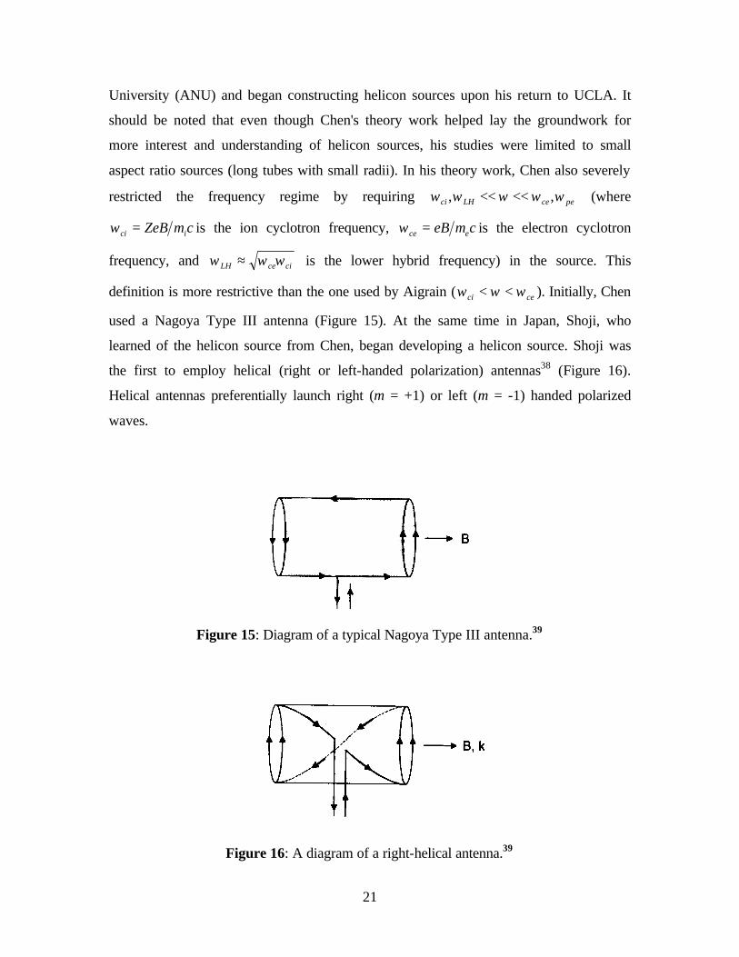
used a Nagoya Type III antenna (Figure 15). At the same time in Japan, Shoji, who
learned of the helicon source from Chen, began developing a helicon source. Shoji was
the first to employ helical (right or left-handed polarization) antennas38 (Figure 16).
Helical antennas preferentially launch right (m = +1) or left (m = -1) handed polarized
waves.
Figure 15: Diagram of a typical Nagoya Type III antenna.39
Figure 16: A diagram of a right-helical antenna.39
22
Chevalier and Chen14 were the first to notice an increase in the plasma density when a
field null was located near the antenna. They observed that the density profile became
much more peaked compared to conifurations without a field null and that the integrated
line density was also larger in the case of the field null. Similar results, including
measurements of an increase in the total volume averaged kinetic energy density, have
been reported by other helicon groups.40
The helicon source has been studied as a possible plasma source for etching of wafers
and helicon sources are now available commercially. Over the last five years, the helicon
source has also become a popular source for basic plasma experiments. Groups that have
recently constructed helicon sources can be found at: Ernst-Moritz-Arndt Univerisität,41
University of California at San Diego (UCSD), Auburn University,42 Oak Ridge National
Laboratory, University of Wisconsin-Madison (UW-Madison), Los Alamos National
Laboratory (LANL), Princeton Plasma Physics Laboratory (PPPL), and WVU.
4.2.2 Helicon Dispersion Relation
The helicon wave is a right-handed, circularly polarized, electromagnetic wave
bounded by an insulating cylinder. The helicon is essentially a whistler wave at a
frequency lower than "traditional" whistler waves. Using the cold plasma dielectric
tensor solution for the right hand, circularly polarized wave, or R wave, a dispersion
relation can be obtained for unbounded plasma waves in the helicon frequency regime.
Starting with Maxwell's time-dependent equations and assuming no external currents
HiE o
rrrωµ=×∇ (25)
EKiH o
rtrr⋅−=×∇ ωε , (26)
where Kt
is the dielectric tensor which includes both plasma and displacement currents.
Kt
is defined as
−=
P
SiD
iDS
K
00
0
0t. (27)
23
where the matrix elements are:
( )LRS += 21 (28)
( )LRD −= 21 (29)
( )∑ +−≡
s cs
psRωωω
ω 2
1 (30)
( )∑ −−≡
s cs
psLωωω
ω 2
1 (31)
∑−≡2
2
1ω
ω psP (32)
Taking the curl of equation. (25), performing Fourier analysis ( ( )txkioeEE ω−⋅=
rrrr) to obtain
the wave equation, and substituting equation (25) into equation (26) yields,
( ) 02
2
=⋅+×× EKc
Ennrtrrr ω
, (33)
whereωck
n
rr
= is the index of refraction and the wave electric field is common in both
terms.
The non-trivial solution to equation (33) requires a solution for arbitrary electric
fields. Writing the solution in terms of the parallel and perpendicular refractive indices,
ωckn ⊥= ||||
rr and ωckn ⊥⊥ =
rryields,
024 =+− ⊥⊥ CBnAn , (34)
where
SA = , (35)
( ) ( )[ ]PSRLPSnB +−+= 2|| , (36)
( )( )LnRnPC −−= 2||
2|| . (37)
The two right circularly polarized solutions to equation (34) are known as the fast
(small ⊥k , high phase velocity, electromagnetic helicon mode) and the slow (large ⊥k ,
slow phase velocity, electrostatic Trivelpiece-Gould (TG) mode). For an R wave, which
is a right-hand circularly polarized wave, the complete dispersion relation, including
collisions, can be written as43
24
( )θωνωω
ω
ω cos1
2
222
ce
pe
i
kcn
−+−== , (38)
where
22||
2⊥+= nnn
kk z=θcos , (39)
22||
2⊥+= kkk . (40)
For the frequency regime of the helicon wave, pececi ωωωω <<<<<< , the dispersion
relation simplifies to
( )νωθω
ωω
ick
ce
pe
−−=
cos22 . (41)
Solving for k yields,
( )
( )νω
ωνωωωω
i
c
ikk
k
pecece
+
+−±
=2
42
1
2
22||
2||
. (42)
The two solutions for k correspond to the helicon mode (minus sign) and the TG mode
(positive sign).44 Rewriting the dispersion relation in terms of frequency leads to two
solutions:
2
22
2
2||
pepe
ce cki
kck
ων
ω
ωω −= (helicon mode), (43)
νωω ik
kce −= || (TG mode). (44)
For ceωω << , only the helicon mode exists. The wave at these frequencies is primarily
electromagnetic, and this is the parameter regime in which most helicon sources operate.
As the frequency approaches the electron cyclotron frequency, the wave becomes more
electrostatic and the TG mode dominates. TG modes will be discussed in more detail
later in this section.
Assuming there are no collisions, equation (43) reduces to
25
2
2||
pe
ce kck
ω
ωω = . (45)
Equation (45) is often referred to as the simple helicon dispersion relation. In Chen's
notation, for small aspect ratio helicon sources ( 2||
2 kk >>⊥ ) the simple dispersion relation
is given by 45
2
2
pe
ce kc
ωαω
ω = (46)
where k corresponds to ||k and α corresponds to k in equation (45). Equation (45)
indicates that the plasma density in a helicon source should be proportional to the
magnetic field and inversely proportional to the antenna driving frequency. As mentioned
previously, the density in a helicon source is observed to be roughly linear with the
magnetic field35 (see Figure 13), though some groups have seen a leveling-off of the
density at higher values of the magnetic field (see Figure 18).37, 46, 47 The plasma density
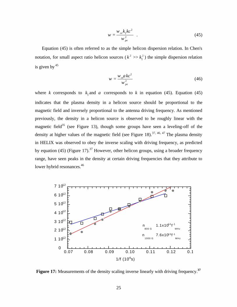
in HELIX was observed to obey the inverse scaling with driving frequency, as predicted
by equation (45) (Figure 17).37 However, other helicon groups, using a broader frequency
range, have seen peaks in the density at certain driving frequencies that they attribute to
lower hybrid resonances.46
0
1 1012
2 1012
3 1012
4 1012
5 1012
6 1012
7 1012
0.07 0.08 0.09 0.10 0.11 0.12 0.13
1/f (10-6s)
n800 G
∼ 1.1x10¹⁴ f -1
MHz
n1000 G
∼ 7.6x10¹³ f -1
MHz
Figure 17: Measurements of the density scaling inverse linearly with driving frequency.37

26
1010
1011
1012
1013
0 500 1000 1500
10 MHz11 MHz13 MHz
Magnetic Field (G)
Figure 18: Measurement of electron density versus magnetic field strength for three different driving frequencies in HELIX. The density increases linearly with the magnetic
field strength and then levels out.
As pointed out in Keiter et al.,37 the simple dispersion relation calculation is not
applicable to helicon sources where the radius is not much smaller than the length
(sources with a moderate aspect ratio). In such cases, the full impact of the boundary
conditions must be included in the analysis. A complete derivation of the helicon wave
magnetic field components in a cylinder was published by Chen et al.,48 and only the
final equations for the wave magnetic fields are reproduced here. The three magnetic
field components are given by:
0)()( =+′+′′zzz BrgBrfB (46)
zzr BikBr
imBk ′+=⊥ γ
α||
2 (47)
zz Br
mkBBk
γαθ
||2 −′−=⊥ (48)
where r∂∂=' and
2
21)(
⊥
′−=
krrf
αα, (49)
27
+
′−−=
⊥
⊥2
22||
||2
22 21)(
k
k
rk
m
r
mkrg
γ
γα
γ, (50)
)()(||
rnkB
er
o
oωµα = , (51)
2
||
1
−=
ck
ωγ , (52)
2||
22 kk −=⊥ α . (53)
Assuming a uniform density profile, ( ) nrn = , and ck <<||ω , (neglecting displacement
currents) the expressions for )(rf and )(rg can be simplified. Equation (46) becomes
01
2
22 =
−+′+′′ ⊥ zzz B
r
mkB
rB (54)
and equation (53) becomes
2||
||0
2 knkB
ek o −
=⊥
ωµ. (55)
Equation (54) is a standard Bessel function differential equation and the boundary
conditions on zB at ar = ( )0=rB due to equation (47) require
( ) ( )akJkakJa
mmm ⊥⊥ ′+= ||0
α (56)
mJ and mJ ′ are the Bessel function of mth order and the derivative of the mth order Bessel
function, respectively. For the case of m = +1:
( ) ( )akJkakJnaB
e⊥⊥ ′+
= 1
2||10
0
00ωµ
(57)
or, rewriting the equation in terms of only ⊥k :
( ) ( )akJ
nB
ekk
akJnaB
e⊥
⊥⊥
⊥ ′
++−
+
= 1
2
00
042
100
0
2
4
0
ωµ
ωµ. (58)
28
Equation (58) can be solved numerically and the ⊥k and ||k for a given set of plasma
parameters compared to measurement. Such high frequency wave field measurements in
HELIX are expected in late 1999.
For the case of m = 0, equation (56) reduces to:
83.3=⊥ak . (59)
Assuming ||kk >>⊥ , and substituting equation (59) into equation (53) yields α = constant.
Substituting this into equation (51) recovers the simple dispersion relation of equation
(45), assuming a uniform density and a small aspect ratio.
4.2.3 Possible Explanations of Efficient Ionization in Helicon sources
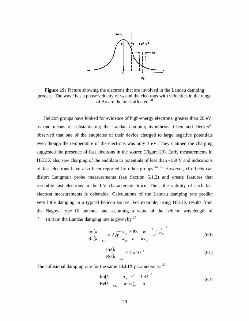
Chen was one of the first to suggest Landau damping as a possible ionization
mechanism in the helicon source. Linear Landau damping is a process where electrons
with velocities approximately equal to the phase velocity of a wave exchange energy with
the wave. Electrons with velocities slightly slower than the phase velocity are sped up
and those slightly faster than the phase velocity are slowed down (See Figure 19). For the
Maxwellian distribution shown in Figure 19, more electrons are traveling slower than the
phase velocity than faster. This leads to a net gain in energy for the particles while the
wave loses energy and is damped. Chen hypothesized that to maximize the ionization
efficiency or density of a small aspect ratio helicon source, the resonant energy of the
electrons must be approximately equal to the optimum electron impact ionization energy
for the gas. For argon, the optimum electron impact ionization occurs for electron
energies of 50 - 100 eV. This led to a period of helicon source design where the antenna
length was chosen to generate phase velocities believed to optimally match the electron
velocities in such a way to achieve the maximum density for a given driving frequency
and magnetic field. Although high-density plasmas were produced in helicon sources
designed to maximize Landau damping,49 little experimental evidence for Landau
damping in helicon sources exists.
29
Figure 19: Picture showing the electrons that are involved in the Landau damping process. The wave has a phase velocity of vp and the electrons with velocities in the range
of ∆v are the ones affected.50
Helicon groups have looked for evidence of high-energy electrons, greater than 20 eV,
as one means of substantiating the Landau damping hypothesis. Chen and Decker51
observed that one of the endplates of their device charged to large negative potentials
even though the temperature of the electrons was only 3 eV. They claimed the charging
suggested the presence of fast electrons in the source (Figure 20). Early measurements in
HELIX also saw charging of the endplate to potentials of less than -150 V and indications
of fast electrons have also been reported by other groups.34, 52 However, rf effects can
distort Langmuir probe measurements (see Section 5.1.2) and create features that
resemble fast electrons in the I-V characteristic trace. Thus, the validity of such fast
electron measurements is debatable. Calculations of the Landau damping rate predict
very little damping in a typical helicon source. For example, using HELIX results from
the Nagoya type III antenna and assuming a value of the helicon wavelength of
8.18≅λ cm the Landau damping rate is given by 37
( )( )
2
v
4
v
83.3v2
Re
Im
−
=
thk
thce
th
LD
ekak
kω
ωω
π (60)
( )( )
310 x 7Re
Im −≈
LDk
k (61)
The collisional damping rate for the same HELIX parameters is: 37
( )( )
2
2
2 83.3
Re
Im
=
a
c
k
k
pe
ei
CDωω
ν (62)

30
( )( )
310 x 2Re
Im −≈
CDk
k (63)
Thus, for typical HELIX operating conditions, Landau damping should be larger than
collision damping. However, both rates are too small to explain the ionization efficiency,
given the input power.
Figure 20: Floating potential versus magnetic field for Chen's experiment. The floating potential of the endplate was as low as -200 V for a field of 40 G. The magnitude of the
floating potential was thought to be caused by fast electrons.51
Recently, Chen et al. estimated an upper limit for Landau damping in a helicon
source.53 Using a gridded energy analyzer and assuming Maxwellian electron
distributions, they measured an electron temperature between 3 eV to 3.35 eV. For a
Maxwellian distribution of such temperatures, the number of fast electrons relative to the
bulk can be estimated. Assuming the electrons capable of the most efficient ionization
have energies of roughly 50 eV, they determined that the 50 eV electrons comprise
roughly 0.02% of the bulk density. Assuming thateVioneVion 350
400 σνσν > , these fast
electrons would still only account for about 10% of the observed ionization.53 Because of
the lack of experimental confirmation, Landau damping is no longer considered a likely
explanation for the high ionization efficiency of helicon sources.
Another possibility is particle trapping.54 Although the process is similar to Landau
damping, the resonant electron energy is determined in a somewhat different fashion. By

31
multiplying the ionization rate curve by a 3 eV Maxwellian distribution function (Figure
21), Degeling et al. determined that 20 eV electrons yield the maximum ionization rate in
an argon plasma with a 3 eV Maxwellian distribution. For appropriate wave frequencies
and wavelengths, these 20 eV electrons can be trapped by a large amplitude rf wave field.
While trapped, the electrons experience simple harmonic motion due to the potential of
the wave and are maintained at their 20 eV kinetic energy. Degeling et al. showed the
number of electrons trapped in the rf wave will grow as the electric field amplitude, and
hence, as the rf power of the antenna is increased. Although this mechanism seems more
likely to result in efficient gas ionization, the available experimental proof is
circumstantial.
Figure 21: Figures from Degeling et al.54 showing a) the distribution function of 3 eV electrons. b) Ionization rate for argon. c) The product of a) and b). The peak velocity
corresponds to an energy of roughly 20 eV d) The mean free path for ionizing collisions.
While considerable attention has been devoted to looking for evidence of Landau
damping or trapped electrons to explain the ionization efficiency, some researchers have
begun to investigate the observed wave characteristics by examining the coupling

32
between helicon waves (modes) and Trivelpiece-Gould (TG) waves (modes).
Experiments have shown that at very low fields (< 100 G), density peaks occur at specific
field strengths.55, 51, 56 Chen originally attributed these density enhancements to electron
cyclotron resonances.56 Although electron inertia had been considered much earlier,57, 58
the possible role of Trivelpiece-Gould (TG) electrostatic modes, which arise from
electron inertia effects, was not considered. Shamrai and Taranov first discussed TG
modes and introduced the terminology of resonances and anti-resonances in a helicon
plasma.59 A resonance occurs when both the helicon wave and the TG wave can exist in
the plasma. An anti-resonance is when either the helicon or the TG wave is not able to
exist in the plasma. In their derivation, they assumed the device has a low aspect ratio and
the wave frequency is greater than the lower hybrid frequency. The TG mode is an
electron-cyclotron wave in a cylinder and has a shorter radial wavelength than the helicon
mode. The TG mode damps with increasing magnetic field, but at low fields, the two
waves have similar mode structure. Thus, the observed density peaks at low B fields may
result from improved coupling to TG modes at particular field strengths.60 At the lower
hybrid frequency, the slow wave changes from an electron wave to an ion wave and only
the helicon mode exists.60 This wave transition might also be responsible for the density
peaks observed at the lower hybrid frequency in higher magnetic field experiments.38, 46
For high plasma density and high magnetic field, the waves will be predominantly
electromagnetic and the helicon component will dominate. For low magnetic fields or
driving frequencies near the cyclotron frequency, electron inertia will dominate, causing
the electrostatic TG wave to dominate.
At this time, there is no conclusive experimental evidence that TG modes propagate
in low field helicon sources. Since the TG modes should dominate when the driving
frequency is near the electron cyclotron frequency and few experiments run at these
parameters, experimental identification of TG modes in low field helicon sources may
not be available for some time.

33
4.3 Space Simulation Chamber
The space simulation chamber, LEIA is large aluminum cylindrical chamber on loan
from Massachusetts Institute of Technology (MIT). LEIA has an inner diameter of 1.8 m
and a length of 4.4 m. There are seven 2.5 m diameter magnet coils spaced along the
length of LEIA to produce a uniform magnetic field. Each magnet contains 20 turns of
0.36" x 0.41" hollow rectangular aluminum tubing. Using a 200 Amp DC EMHP power
supply, the magnetic field can be varied from 0 to 70 Gauss. The magnetic field in LEIA
is given by:
HL IIB 022.33.09.1 ++−= (64)
where LI is the current in the LEIA coils and HI is the current in the HELIX coils. Figure
22 and Figure 23 show the radial and azimuthal magnetic field profiles in LEIA. The
magnetic field in HELIX significantly influences the magnetic field strength in LEIA
near the bellows joining the two devices (z > 300 cm).
0
10
20
30
40
50
0 50 100 150 200 250 300 350 400
B (HELIX at 600 G)
B (HELIX at 400 G)
LE
IA M
agne
tic F
ield
(G
)
Distance (cm)
Figure 22: Azimuthal magnetic field profile in LEIA. Note that as the field in HELIX is increased, the magnetic profile becomes steeper for z > 300 cm.

34
0
5
10
15
20
25
-150 -100 -50 0 50 100 150
LE
IA M
agne
tic F
ield
(G
)
Radius (cm)
Figure 23: Radial Profile of magnetic field in LEIA.
At the far end of LEIA are two Balzers TMU 1600 turbomolecular pumps. A nearby
pressure gauge is used to measure the neutral pressure in LEIA. The differential pumping
design creates a neutral pressure gradient in LEIA. Thus, the neutral pressure in LEIA is
typically five to ten times lower than in HELIX.
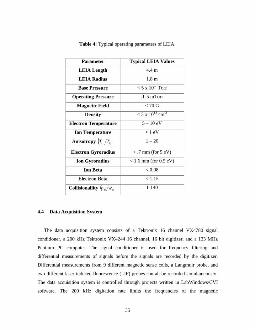
Typical operating parameters for LEIA are shown in Table 4. The magnetic field
strengths in HELIX and LEIA, the pressure and the rf power can be manipulated to
control the plasma density and ion temperature in LEIA. The mechanism responsible for
the large ion temperatures observed in LEIA is currently unknown but is under
investigation.
35
Table 4: Typical operating parameters of LEIA.
Parameter Typical LEIA Values
LEIA Length 4.4 m
LEIA Radius 1.8 m
Base Pressure < 5 x 10⁻⁷ Torr
Operating Pressure .1-5 mTorr
Magnetic Field < 70 G
Density < 3 x 1013 cm-3
Electron Temperature 5 – 10 eV
Ion Temperature < 1 eV
Anisotropy ( )||ii TT⊥ 1 – 20
Electron Gyroradius < .7 mm (for 5 eV)
Ion Gyroradius < 1.6 mm (for 0.5 eV)
Ion Beta < 0.08
Electron Beta < 1.15
Collisionallity ( )ciii ων 1-140
4.4 Data Acquisition System
The data acquisition system consists of a Tektronix 16 channel VX4780 signal
conditioner, a 200 kHz Tektronix VX4244 16 channel, 16 bit digitizer, and a 133 MHz
Pentium PC computer. The signal conditioner is used for frequency filtering and
differential measurements of signals before the signals are recorded by the digitizer.
Differential measurements from 9 different magnetic sense coils, a Langmuir probe, and
two different laser induced fluorescence (LIF) probes can all be recorded simultaneously.
The data acquisition system is controlled through projects written in LabWindows/CVI
software. The 200 kHz digitation rate limits the frequencies of the magnetic
36
measurements to 100 kHz. For magnetic fluctuation measurements, 2048 points are
recorded, giving a frequency resolution of 97 Hz. 1000 points are recorded for the
Langmuir probe and LIF measurements.

37
5 DIAGNOSTICS
The LEIA diagnostics used for these experiments included a Langmuir probe, two LIF
probes separated axially, and nine magnetic sense coils separated axially, radially, and
azimuthally. The nine magnetic sense coils can determine the wavelengths of
electromagnetic instabilities in LEIA in the r , θ , and z directions. The LIF, magnetic,
and Langmuir probes were mounted on linear motion Velmex stages, capable of sub-
millimeter position resolution. The probes perturbed the plasma somewhat, but only
seemed to affect downstream measurements on the same field line. The upstream
measurements were not affected by the downstream probes. In HELIX, the only
diagnostic used was LIF.
5.1 Langmuir Probe
A Langmuir probe is essentially a conductor inserted into a plasma. The conductor is
then biased with a voltage and the current to the probe measured.61 The relationship
between the biasing voltage and the collected current is referred to as an I-V
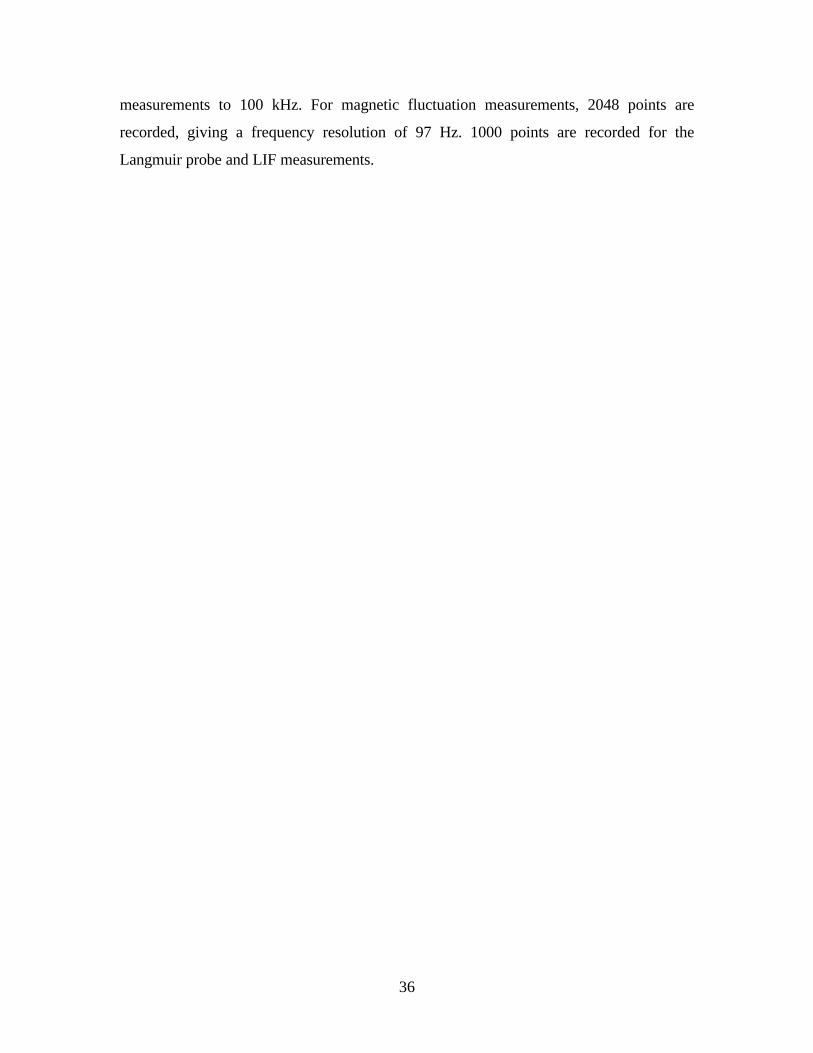
characteristic, or an I-V trace. A typical I-V trace is shown in Figure 24.
38
-0.002
-0.001
0
0.001
0.002
0.003
0.004
0.005
0.006
-100 -50 0 50 100
Cur
rent
(A
)
Voltage (V)
Ion Saturation Current
ElectronSaturation
Current
FloatingPotential
Plasma Potential
Figure 24: Hypothetical Langmuir probe trace.
When a Langmuir probe is placed into a plasma, the probe typically becomes
negatively charged. This is because the electrons are usually more mobile in the plasma
than the positive ions and thus the electron flux to the probe is greater than the ion flux.
The voltage that an unbiased probe charges to is called the floating potential. As the
probe is biased more negative than the floating potential, the probe collects ion current.
Eventually, a limit is reached when the probe is collecting as much ion current as it can
possibly collect given the plasma density and temperature. This is known as the ion
saturation current. If the probe is biased more positive than the floating potential,
electrons are collected. As seen in Figure 24, right after the floating potential the I-V
trace takes a sharp turn upward. The bend is also referred to as the "knee". As the positive
bias is increased on the probe, eventually the collected electron current reaches a plateau.
This is referred to as the electron saturation current.

39
5.1.1 Determination of electron density and temperature
Assuming the plasma is collisionless and there is no magnetic field, the current in the
region around the knee can be approximated by: 61
( )
−−
−
= ∞ 2
1exp
)(exp
2
2
1 21
21
p
s
e
po
e
i
i
epo A
A
T
VVe
m
m
m
TeAnVI
π (65)
where em is the electron mass, im is the ion mass sA is the area of the sheath, pA is the
surface area of the probe, pV is the plasma potential and oV is the applied voltage. The
sheath around a Langmuir probe is a region of space a few Debye lengths thick. The
sheath is a region of spatially varying potential and is created when the ions in the plasma
Debye shield the potential applied to the probe.62 The two unknowns in equation (65) are
∞n , the electron density far from the probe, and eT , the electron temperature. The
derivative of the current with respect to the bias voltage is:
( ))( po
sisi
eo VVd
dIII
T
e
dV
dI
−+−= (66)
where isi eJI −= and
( ) 21
iepi mTAnJ ∞= (67)
Since the ion saturation current, siI , is relatively constant, o
si
o dVdI
dVdI >> .
Therefore, eT can be approximated by
( ))( po
sie VVd
dIIIeT
−−= . (68)
Once the electron temperature is obtained from the slope of the I-V characteristic, it is
straightforward to use equation (67) to calculate the electron density of the plasma from
the measured ion saturation current. As the pV was not determined, fV was used.
Langmuir probes are often used in plasmas with a strong magnetic field. The charged
particles no longer move in straight lines but in gyro-orbits. Motion across field lines is
restricted while motion along the field lines is basically the same as without a magnetic
field. The electrons are more strongly affected than the ions because their gyro-orbits are

40
much smaller than that of the ions (assuming the electrons and ions are approximately the
same temperature). Thus, the electron saturation current decreases with a stronger
magnetic field.61 For cylindrical probes, the importance of magnetic field effects scales
with the ratio of the gyro-radius to the probe radius. When this ratio is much less than one
for a particle species, then that species is impeded from reaching the probe and the
equations (65) through (68) must be modified by including collisions and estimates of
cross field transport.61 For LEIA, assuming a typical field (35 G), an ion temperature of
0.3 eV, and electron temperature of 5 eV, the ion gyro-radius is roughly 2.5 mm and the
electron gyro-radius is about 1.5 mm. Since the Langmuir probes used have radii of 0.5
mm, both species have a gyroradius to probe radius ratio larger than 1. Therefore, the
field free formulae should provide a good approximation for the electron temperature and
the density in LEIA.
5.1.2 Langmuir Probe Design
Plasmas created by a sinusoidal, time-varying signal can influence the I-V trace of a
Langmuir probe by distorting the electron retardation region and also shifting the floating
potential more negative.63 For Maxwellian electron distributions, an accurate electron
temperature can be obtained from the average electron current as long as the electron
current stays in the exponential region of the I-V characteristic, i.e., near the knee.
However, if the rf potential forces the electron current outside of the exponential region,
then the electron temperature can be overestimated by traditional analysis methods.
Besides electron temperature overestimates, the I-V characteristic can also be distorted by
the rf to resemble the I-V characteristic of a Maxwellian distribution with a hot tail.63, 64
To compensate for this, Sudit and Chen developed a method of probe construction to
eliminate the rf influence on the Langmuir probe.65 Their method is similar to a method
developed by Godyak et al..66
41
101
102
103
104
105
100 101 102 103 104 105 106 107 108
Impe
denc
e (O
hms)
Frequency (Hz)
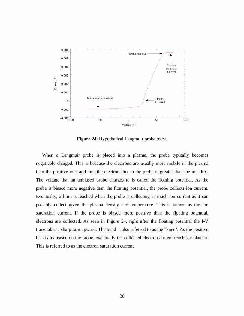
Figure 25: Typical frequency response of the Langmuir probe used in LEIA.
Physically, there are two modifications made to a standard Langmuir probe. The first is
the addition of a floating electrode.65 The electrode is exposed to the plasma potential
fluctuations and connected to the Langmuir probe tip via a large capacitor. This helps to
lower the sheath impedance and forces the Langmuir probe tip follow the plasma
potential oscillations; thereby reducing the distortion in the trace. The second
modification is a chain of rf chokes. These are placed after the probe tip, but before the
current is measured. The chokes increase the impedance of the circuit at the rf frequency.
The impedance as a function of frequency for a typical Langmuir probe used in LEIA is
shown in Figure 25.
In LEIA, a Keithley 2400 SourceMeter is used to measure the I-V characteristic of
the Langmuir probe from -50 V to +50 V. The SourceMeter is controlled through a GPIB
interface installed in the PC. A schematic drawing of the Langmuir probe used in LEIA is
shown in Figure 26. The probe is mounted on a motorized Velmex drive that allows the
radial profile of the electron temperature and density to be measured at a particular z
position. To measure the plasma density at different axial positions, the probe is

42
physically moved to another port. A typical Langmuir probe trace from LEIA is shown in
Figure 28.
double O-ring sealprobe tip assemblyKF 40 vacuum coupling
electrical feedthrough
Keithly 2400sourcemeterKeithly 2400sourcemeter
GPIB
cardPC
(see Figure 27 for details)
Figure 26: Schematic drawing of the Langmuir probe and measurement circuit.
Figure 27: Photograph of the Langmuir probe head. The exposed graphite tip is 2 mm long and runs the length of the alumina tube into the boron-nitride cap. The capacitor

43
between the graphite tip and a small copper rod has a value of approximately 5 nF. Five inductors having values between 15 and 270 µH are placed in series behind the capacitor.
-1 10-4
0 100
1 10-4
2 10-4
3 10-4
4 10-4
5 10-4
-60.0 -40.0 -20.0 0.0 20.0 40.0 60.0
Cur
rent
(A
)
Voltage (V)
Isat
Te= 5.8 eV
Figure 28: Typical Langmuir probe trace in LEIA.
Electron temperatures in LEIA are typically 5 - 7 eV. These values are somewhat
higher than the 3-5 eV temperatures reported by other helicon groups. The likely culprit
is differences in the rf compensation of the Langmuir probes. The chokes used in the
LEIA probes are not optimized for the 8 - 10 MHz rf frequencies used in HELIX. In
addition, there might be some electron heating as the plasma expands from HELIX into
LEIA and the plasma density drops.
44
5.2 Laser Induced Fluorescence
One of the key diagnostics used in these experiments is laser induced fluorescence
(LIF). LIF was first suggested as a plasma diagnostic in 1968 by Measures.67 LIF is based
upon the selective excitation of an atomic transition by the absorption of laser radiation of
the appropriate wavelength. LIF can be used to observe the following:
(i) Ion and atomic velocity (zeroth order) distribution functions (hence ion and
atomic temperatures) and densities;
(ii) Ion and atomic particle trajectories;
(iii) Electron temperature from the relative populations of the excited levels;
(iv) The vector direction and magnitude of the local magnetic field by means of the
Zeeman effect;
(v) The effective ion charge and the local electric field by means of the Stark effect;
(vi) Ion and atomic first order distribution functions. This can yield the value of the
perturbing potential and lead to wavelength measurements of electrostatic
waves.68, 69
In this work, only techniques for (i) will be discussed in detail. A discussion of
technique (ii) can be found in the work of McChesney.70 Discussion of techniques (iv)
and (v) can be found in the work of Moore et al.71 and West et al.,72 respectively.
Technique (iii) can only be applied to high-density plasmas, where the ions are in local
thermodynamic equilibrium.
The absorption and emission frequencies of an atom or ion moving relative to a
radiation source are Doppler shifted by an amount proportional to the component of
velocity along the radiation direction. During a typical LIF measurement, the frequency
of a narrow bandwidth laser is swept across a collection of ions or atoms that have a
thermally broadened velocity distribution. The absorption spectrum for the entire
ensemble of atoms or ions has associated with it a width and a shift from the natural
frequency. The width is used to determine the temperature and the shift to determine flow
velocity of the particle distribution. The LIF system used in these experiments consists of
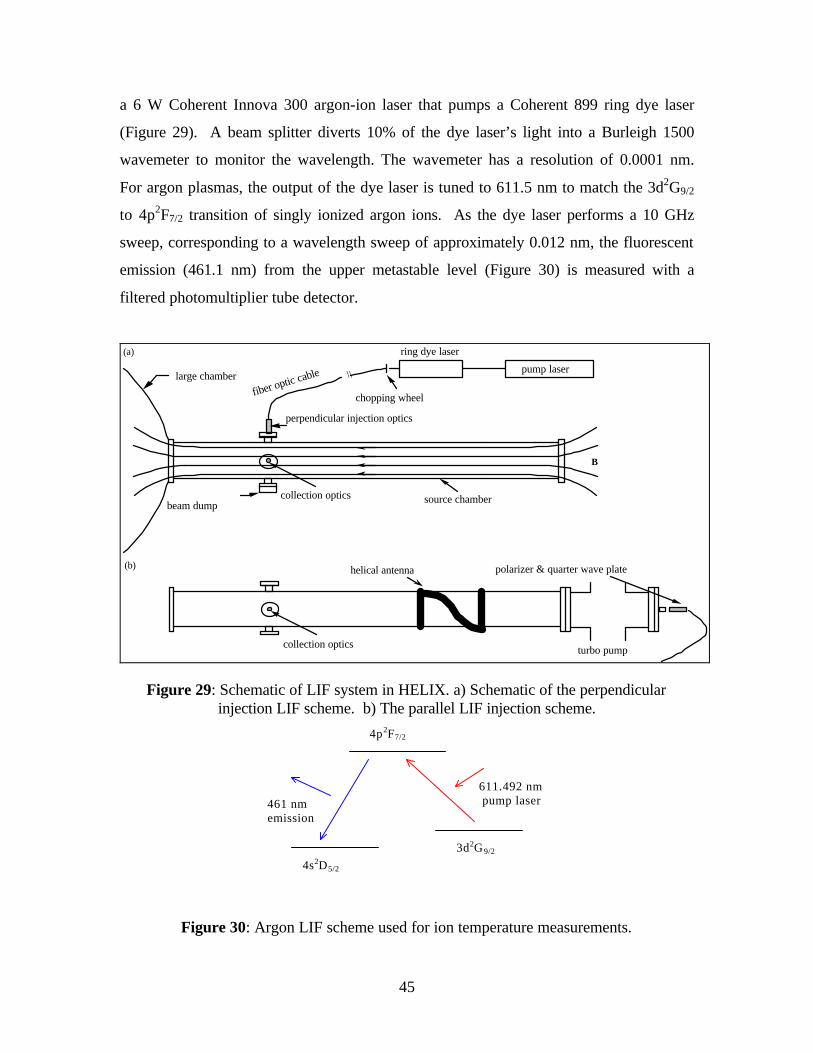
45
a 6 W Coherent Innova 300 argon-ion laser that pumps a Coherent 899 ring dye laser
(Figure 29). A beam splitter diverts 10% of the dye laser’s light into a Burleigh 1500
wavemeter to monitor the wavelength. The wavemeter has a resolution of 0.0001 nm.
For argon plasmas, the output of the dye laser is tuned to 611.5 nm to match the 3d2G9/2
to 4p2F7/2 transition of singly ionized argon ions. As the dye laser performs a 10 GHz
sweep, corresponding to a wavelength sweep of approximately 0.012 nm, the fluorescent
emission (461.1 nm) from the upper metastable level (Figure 30) is measured with a
filtered photomultiplier tube detector.
B
(a)
\\
chopping wheel
ring dye laser
pump laser
perpendicular injection optics
collection optics beam dump
(b)
collection optics
source chamber
polarizer & quarter wave plate
fiber optic cable
turbo pump
helical antenna
large chamber
Figure 29: Schematic of LIF system in HELIX. a) Schematic of the perpendicular injection LIF scheme. b) The parallel LIF injection scheme.
4p2F7/2
4s2D5/2
3d2G9/2
611.492 nm pump laser 461 nm
emission
Figure 30: Argon LIF scheme used for ion temperature measurements.

46
The filter in front of the photomultiplier has a 1.0 nm passband centered around the
emission line. The output of the dye laser is chopped at 1 kHz. The chopping signal is
used as the reference for a Stanford Research SR830 lock-in amplifier that monitors the
photomultiplier tube signal and distinguishes the fluorescence signal from the intense
background emission at the same wavelength using phase synchronous detection. The
amplified signal from the SR830 and a measurement of the laser power during the sweep
are sent to the Tektronix VXI 4244 digitizer. The LIF signal is normalized by the laser
power measurement and is then fitted to a single Gaussian distribution to determine the
ion temperature and the center frequency of the ion distribution.
In HELIX, perpendicular and parallel components of the argon ion temperature are
obtained by injecting the laser light into the plasma perpendicular and parallel to the
magnetic field, respectively. In both cases, the emitted light is collected perpendicularly
to the magnetic field (Figure 29). For perpendicular measurements, only the linearly
polarized π transitions are excited. For the parallel measurements, two circularly
polarized σ transitions are excited. Because the laser light is transported through a
multimode fiber, the polarization of the laser is not preserved. Since the Zeeman splitting
of the σ lines is on the order of the thermal broadening in HELIX, Zeeman splitting for
parallel measurements cannot be ignored. By introducing a combination of a linear
polarizer followed by a quarter wave plate into the parallel injection optics, a single
circular polarization is selected and only one of the two σ transitions is excited. The
additional optical components reduce the overall intensity of the laser light and lower the
signal-to-noise ratio for parallel ion temperature measurements.
In LEIA, LIF is accomplished with two different LIF probes. One is a re-entrant
probe that contains miniature collection optics in a glass tube inserted into the plasma
(Figure 31a). The laser is injected from an external port and aligned with the collection
optics (Figure 31b). The other is a fully in-situ probe (Figure 32). The in-situ design
allows the injection and collection optics to be placed much closer to each other (~5cm)
than if external ports on the machine were used, thereby increasing the signal to noise
ratio. Another advantage of the in-situ LIF probe is that it can be used to measure radial
profiles of the ion temperature and perform tomographic surveys of the plasma. Since the

47
magnetic field in LEIA is on the order of 50 G, Zeeman splitting of the argon lines in
LEIA is not a concern.
1 mm core silica fiber
5 cm focal length lens 1/2 " shaftA)
B)
detect ion volume ~ 3 mm x 5 mm
re-entrant probe
injection optics
typical separation ~ 5-10 cm
Figure 31: a) Schematic of re-entrant LIF probe. Emission from the 461.1 nm line is focused into the fiber with a 1/4" plano-convex lens. The fiber is connected to the same filtered PMT that is used for the HELIX measurements. b) Configuration of re-entrant probe inside of LEIA for T⊥ measurement. The laser light is injected from the top of
LEIA, and focused at the center of the plasma. The re-entrant probe collects the light emitted by the ions in the region defined by the intersection of the collection and
injection focal paths.
The two LIF probes are located approximately 65 cm apart, thereby allowing the ion
temperature to be studied at two axial positions in the plasma. The re-entrant probe is

48
placed closer to the plasma source and is referred to as the upstream probe. The in-situ
probe is referred to as the downstream probe.
Figure 32: Picture of the head of the radially scanning, in-situ LIF probe.

49
detection volume 600 µ core fiber
200 µ core fiber
collection optics
injection optics
Figure 33: Schematic of the in-situ LIF probe. The laser light (611.5 nm) is injected into the plasma through the dog-leg and the emission (461.1 nm) is focused with lenses into a
600 µ core fiber. The probe can move radially and also rotate about the shaft axis.
5.2.1 Line Broadening Mechanisms
Spectral lines always have some finite width due to a variety of linewidth broadening
mechanisms. Such mechanisms include: natural broadening, Doppler broadening,
pressure broadening, Zeeman broadening, power broadening and instrumental
broadening.
5.2.1.1 Natural Linewidth73
The Heisenberg uncertainty principle is used to determine the natural linewidth of a
transition between two levels. For an excited state, iE , with a mean lifetime of iτ , the
uncertainty is given by:

50
( ) ii hE τπ 12 −=∆ . (69)
If the lower level is not the ground state, but another excited state, kE , with a mean
lifetime of kτ , the uncertainties of both levels contribute to the total uncertainty,
ki EEE ∆+∆=∆ . (70)
Rewriting equation (70) in terms of the uncertainty in the angular frequency and
including transitions from any level to either of the two levels of interest leads to
∑∑ +=∆n nkm miik AAω , (71)
where i and k are the levels of interest, m and n are all levels excluding the level of
interest, and miA and nkA are the Einstein coefficients for each transition. Since in this
case the lower 2923 Gd state is a metastable state, all of the transitions originating from
this level have a very small spontaneous transition probability when compared to a
transition originating from the upper 2724 Fp . Therefore, the total uncertainty in the
angular frequency for this atomic transition is given by:
∑≈∆m miik Aω . (72)
The Einstein coefficients for the argon ion levels used for LIF are tabulated73 and the
uncertainty in the angular frequency is approximately
16 s1018.1 −×≅∆ ikω (73)
In terms of wavelengths,
nm1033.2 5−×≅∆∴ naturalλ (74)
5.2.1.2 Doppler Broadening73
Doppler broadening is caused by the random thermal motion of a radiating or
absorbing atom or ion. If the velocity component of the radiating particle parallel to the
direction of observation is v, then the frequency is shifted due to the Doppler effect by
the amount:

51
cv 0νν ±=∆ , (75)
where 0ν is the unshifted frequency. Assuming that the particle motion is purely thermal
in nature, a Maxwellian distribution function can be used for the emitters/absorbers.
( ) ( )[ ]iBoi Tkm
iB
i eTk
mf 2v-v 2
2v −=
π, (76)
where iT is the ion temperature and ov is the average ion velocity. The light intensity at a
particular frequency is proportional to the number of particles at that frequency, i.e.
( ) ( ) vv dfdI ∝νν , where ( )νI is the line shape. For a Maxwellian collection of
emitters/absorbers, the Doppler-broadened line shape is:61
( ) ( ) ( )[ ]22th
22 v2 oo co eII ννννν −−= (77)
where iBth mTk=2v and oν is the frequency corresponding to the center velocity of the
ion distribution. Setting the exponential term to ½ yields the full width at half maximum
(FWHM) of the linewidth:
( ) 2ln2v021 cthνν =∆ . (78)
Rewriting this in terms of temperature:
( )( ) 2ln22021 mTkc iBνν =∆ (79)
and, in terms of wavelengths:
( )( ) 2ln22021 mTkc iBλλ =∆ . (80)
For room temperature ( eV 0.03=iT ) ions,
nm 101 3−×≈∆ dopλ . (81)
5.2.1.3 Pressure Broadening73
Pressure broadening includes the effects of collisions with neutral particles (van der
Waals broadening), resonance interaction between like particles (resonance broadening)
and collisions with charged particles (Stark broadening). The first two mechanisms are
important for weakly ionized plasmas (< 1% ionized),74 while the last is important for

52
highly ionized, high-density plasmas. HELIX is a highly ionized, high-density plasma
source, so only Stark broadening might have a significant effect on the linewidth. LEIA,
though slightly less ionized than HELIX, is still ionized enough to ignore all pressure
broadening except for Stark broadening. The full width at half maximum (FWHM)
associated with the Stark effect is given by: 75
( )[ ]216134141621 s 1002.111075.11102 −−−− ×−×+×≈∆ eeee Tnnn αωλ . (82)
Where ω is the electron impact half width parameter, α is the ion broadening parameter,
en is the electron density and eT is the electron temperature. The parameters ω and α
have been tabulated for numerous Ar ion transitions as a function of electron
temperature.75 Assuming eV 5=eT , -314 cm 10 =en and approximating values for α
and ω,73 the Stark broadening is approximately:
nm1016.1 5stark
−×≈∆λ (83)
5.2.1.4 Zeeman Broadening73
The interaction of the magnetic moment of an electron with an applied magnetic field
results in the splitting of an observed spectral line. The “normal” Zeeman effect occurs
when a singlet line splits into three polarized components. The “anomalous” Zeeman
effect occurs when a line is split into a group of four or more components.
When a spectral line splits in a magnetic field, the Zeeman components are polarized
either parallel or perpendicular to the magnetic field. The parallel components are
referred to as π components, or π lines, and the perpendicular components are referred to
as σ components, or σ lines. The Zeeman components are always shifted symmetrically
about the position of the undisplaced line. For the “normal” Zeeman effect, the three
components arising from a line of frequency f, have frequencies of f, ff ∆+ , and
ff ∆− . The undisplaced line is the π line and the two displaced lines are the σ lines. The
π line is linearly polarized along the magnetic field direction and the σ lines are circularly
polarized perpendicular to the magnetic field. The two σ components rotate in opposite
directions.
53
The number of energy levels, or degree of splitting, obtained in a magnetic field
depends on the total angular momentum value (2J+1), of the transition states. J = 1 gives
rise to the normal Zeeman effect. In general, the energy difference between the different
lines due to the interaction between the magnetic moment and the magnetic field, B, is:
jjB MBgE µ=∆ , (84)
where, ( ) 14 −= eB meh πµ is the Bohr magneton, jM is the magnetic orbital quantum
number, B is the magnetic field in Gauss, and jg is the Lande factor. The Lande factor is
given by:
( ) ( ) ( )[ ] ( ) 121111 ++−++++= JJLLSSJJg j (85)
where J is the total angular momentum, S is the spin angular momentum, and L is the
orbital angular momentum for the electron energy level. Thus, the energy difference
between two levels is:
( )2211 MgMgBE B −=∆ µ . (86)
Rewriting this expression in terms of wavelength
( ) ( )221112 MgMgchBB −=∆ −λµλ . (87)
Calculation of each of the terms of equation (87) for the appropriate argon ion parameters
is described in reference 73. For a field of 100 G, the largest Zeeman broadening due to
the splitting of the σ lines is approximately
nm 106.2 5−×=∆ zeeλ . (88)
5.2.1.5 Power Broadening73
Power broadening occurs when the stimulated photon emission rate equals the photon
absorption rate and both are greater than the spontaneous emission rate. When saturation
occurs, the power residing in the wings of the laser becomes important, resulting in
photon absorption far from the laser central line.76 Goeckner and Goree developed
empirical equations that can be used to estimate the effects of power broadening.77
Goeckner and Goree's experiments used a 1 GHz bandwidth, pulsed laser (17 ns) tuned to
the same argon transition used for LIF in HELIX and LEIA argon plasmas. Since the

54
linewidth of the laser described in section 5.2 is approximately 1 MHz, significantly less
broadening is expected than with a 1 GHz linewidth laser. Assuming the laser beam has a
diameter of about 2 mm and a maximum power of 100 mW, an upper bound for the
effects of power broadening is given by
nm 101 4−×≤∆ powerλ . (89)
5.2.1.6 Instrumental Broadening73
There are two types of instrumental broadening; one associated with the laser
linewidth, and one associated with the dispersion of the light detection system. The
emission light is measured with a passband filtered (±1 nm) photomultiplier tube. Thus,
there is no dispersion in the collection system. The laser bandwidth for the Coherent 899
Ring laser is less than 1 MHz, which in terms of wavelengths is
nm 1025.1 6−×≤∆ laserλ (90)
for a central wavelength of 611.53 nm.
5.2.1.7 Comparison of Broadening Mechanisms
Because the Doppler FWHM is used to determine the ion temperature in these
experiments, any of the other mechanisms that artificially broaden the LIF lineshape must
be accounted for before the ion temperature can be estimated.

55
Table 5: Approximate linewidths associated with different lineshape broadening mechanisms
listed in order of significance.
Broadening Mechanism FWHM value (nm)
Doppler Broadening ~ 1.0 x 10⁻³
Zeeman Broadening (σσ lines) ≤ 2.6 x 10⁻⁴
Power Broadening < 1.0 x 10⁻⁴
Pressure Broadening ~ 1.2 x 10⁻⁵
Natural Linewidth ~ 2.3 x 10⁻⁵
Instrumental Broadening ~ 1.3 x 10⁻⁶
As shown in Table 5, most of the possible lineshape broadening mechanisms have a
much smaller FWHM value than Doppler broadening. However, in HELIX, Zeeman
broadening can be as much as 25% of the Doppler broadening. As mentioned previously,
a linear polarizer followed by a quarter waveplate is used to select a single circular
polarization for parallel LIF measurements. For perpendicular LIF measurements, a
linear polarizer in the collection optics is used to select the linearly polarized π lines. The
power broadening is an extreme overestimation and experimental tests have show that the
laser power can be changed by a factor of three and the measured distribution function is
not affected (Figure 34). A typical LIF trace is shown in Figure 35. The LIF signal is well
fit by a single Maxwellian distribution function.

56
0.00
0.08
0.16
0.24
0.32
0.40
0.48
0.56
0.64
0.0 100.0 200.0 300.0 400.0
Ion
Tem
pera
ture
(eV
)
Laser Power (mW)
Figure 34: Argon ion temperature as a function of dye laser power with 10 % error bars. The data were taken at a pressure of 7.1 mTorr, rf frequency of 8.5 MHz, rf power of 600
W and B ~ 1 kG.
0.00
0.01
0.02
0.03
0.04
0.05
0.06
0.07
-8.0 -6.0 -4.0 -2.0 0.0 2.0 4.0 6.0 8.0
LIF
Sig
nal (
arb
units
)
Frequency Shift from Center of Argon Ion Line (GHz)
Figure 35: A typical LIF trace (solid line) for a perpendicular measurement in LEIA. The ion temperature from the fit (dashed line) is 0.21 eV in this case.

57
5.3 Magnetic Probe
5.3.1 Magnetic probe construction and calibration
A standard magnetic sense coil is made from a loop, or loops, of wire. If the magnetic
field passing through the loop of wire is time-dependant, then, from Faraday's Law, a
voltage will be induced around the loop. If the voltage is measured over a period of time,
a time series record of the signal can be recorded. Using Fourier analysis, spectral
features can then be identified and examined. Comparing the signals from two coils
provides a measurement of the phase shift between the two coils. The phase shift at a
particular frequency divided by the distance between the probes yields the wavenumber,
k, of the magnetic fluctuation.
2
1 4
3
6
7
Aluminum foil
Twisted magnet wire
Coil form
Boron nitride cap
z
r
Figure 36: Magnetic probe diagnostic used in LEIA. There are two coils not seen in this view, one on the backside of the middle leg and one on the backside of the right leg. Each
coil is wound with nominally two hundred turns of 35 gauge copper magnet wire on a barbell shaped piece of boron nitride. The shafts are stainless steel and each coil is
capped with a thin piece of aluminum foil and a boron nitride cover.

58
A schematic of the magnetic probe used in LEIA is shown in Figure 36. The design
of the probe allows three-dimensional measurements of the wavenumber spectrum. The
coils are identified as coils 1-10. Coils 1, 3 and 6 are along the z-direction, coils 2, 4, and
7 are along the r-direction, and coils 5, 8, and 9 are in the θ-direction. As coil 5 was
defective, no data was available from coil 5. Coil 10 was a single radial coil placed on
another probe farther upstream from the other 9 coils.
Figure 37: A picture of the magnetic fluctuation probe inside LEIA.
The magnetic probe was calibrated to determine the inherent phase shift in each coil
due to the length of wire, the Tektronix 4780 signal conditioner and the Tektronix 4244
digitizer. A measurement of the inherent phase shift is required to ensure that any
measured phase shifts between two coils are real and not electronic artifacts. A solenoidal
59
coil driven with a HP function generator was used to generate a time-varying magnetic
field for calibrating the coils. Each magnetic fluctuation sense coil was placed within the
solenoid and the solenoid was then ramped in frequency, starting at 100 Hz and ending at
100,000 Hz. At each frequency step, the amplitudes of the current through the solenoid
(the reference signal) and the signal detected by the magnetic sense coil were measured.
The phase shift between the two signals at each frequency was used as a measure of the
inherent phase shift in each coil relative to the calibration coil. The relative amplitudes of
the signals were also used to determine the effective area of the coils as a function of
frequency. The voltage induced in the magnetic sense coil is given by:
)()( tBNAtVcoil&= , (91)
where N is the number of turns on each coil, A is the area of each coil and B& is the
magnitude of the time derivative of the magnetic field. Since ( ) )2sin( ftfBB o π= ,
( ) )2cos(2 ftffBB o ππ=& . ( ) ( ) nfIfB osourceo µ= , where ( )fIsource is the frequency
dependent output current of the function generator and n is the turns per unit length of the
solenoid. The relationship between ( )fBo and ( )fIsource as a function of frequency was
measured with a Walker Scientific model MG-50 gaussmeter. Therefore, at anytime t,
( ) )2cos(2 ftNAfBtV ocoil ππ= . (92)
In terms of the peak values, the effective sense coil area as a function of the frequency
is optp fBVNA π4= . Plots of the area and phase shift of each coil versus frequency are
shown in Figure 38. Each coil was nominally wrapped with 200 turns of 35 gauge copper
magnet wire.

60
10-7
10-6
10-5
10-4
0 2 104 4 104 6 104 8 104 1 105
Coi
l Are
a (m
2 )
Frequency (Hz)
Coil 1
-3.0
-2.0
-1.0
0.0
1.0
2.0
3.0
0 2 104 4 104 6 104 8 104 1 105
Pha
se (
Rad
ians
)
Frequency (Hz)
Coil 1
10-7
10-6
10-5
10-4
0 2 104 4 104 6 104 8 104 1 105
Coi
l Are
a (m
2 )
Frequency (Hz)
Coil 2
-3.0
-2.0
-1.0
0.0
1.0
2.0
3.0
0 2 104 4 104 6 104 8 104 1 105
Pha
se (
Rad
ians
)
Frequency (Hz)
Coil 2
10-7
10-6
10-5
10-4
0 2 104 4 104 6 104 8 104 1 105
Coi
l Are
a (m
2 )
Frequency (Hz)
Coil 3
-3.0
-2.0
-1.0
0.0
1.0
2.0
3.0
0 2 104 4 104 6 104 8 104 1 105
Pha
se (
radi
ans)
Frequency (Hz)
Coil 3

61
10-7
10-6
10-5
10-4
0 2 104 4 104 6 104 8 104 1 105
Coi
l Are
a (m
2 )
Frequency (Hz)
Coil 4
-3.0
-2.0
-1.0
0.0
1.0
2.0
3.0
0 2 104 4 104 6 104 8 104 1 105
Pha
se (
Rad
ians
)
Frequency (Hz)
Coil 4
10-7
10-6
10-5
10-4
0 2 104 4 104 6 104 8 104 1 105
Coi
l Are
a (m
2 )
Frequency (Hz)
Coil 6
-3.0
-2.0
-1.0
0.0
1.0
2.0
3.0
0 2 104 4 104 6 104 8 104 1 105
Pha
se (
Rad
ians
)
Frequency (Hz)
Coil 6
10-7
10-6
10-5
10-4
0 2 104 4 104 6 104 8 104 1 105
Coi
l Are
a (m
2 )
Frequency (Hz)
Coil 7
-3.0
-2.0
-1.0
0.0
1.0
2.0
3.0
0 2 104 4 104 6 104 8 104 1 105
Pha
se (
Rad
ians
)
Frequency (Hz)
Coil 7
10-7
10-6
10-5
10-4
0 2 104 4 104 6 104 8 104 1 105
Coi
l Are
a (m
2 )
Frequency (Hz)
Coil 8
-3.0
-2.0
-1.0
0.0
1.0
2.0
3.0
0 2 104 4 104 6 104 8 104 1 105
Coil 8
Pha
se (
Rad
ians
)
Frequency (Hz)
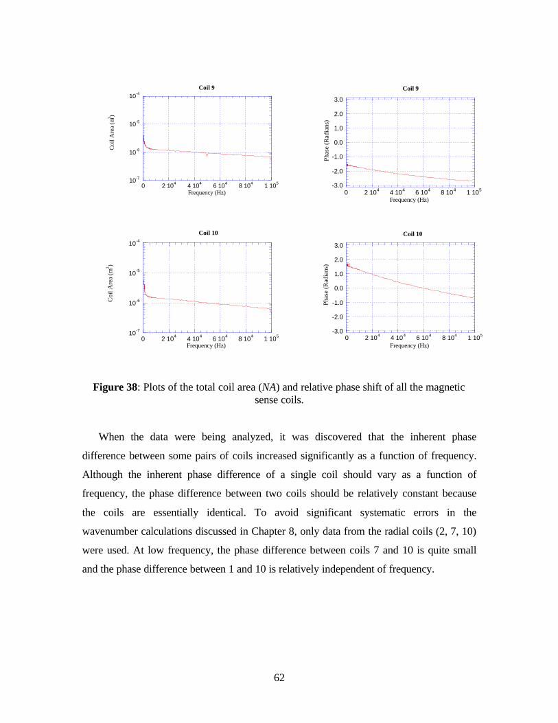
62
10-7
10-6
10-5
10-4
0 2 104 4 104 6 104 8 104 1 105
Coi
l Are
a (m
2 )
Frequency (Hz)
Coil 9
-3.0
-2.0
-1.0
0.0
1.0
2.0
3.0
0 2 104 4 104 6 104 8 104 1 105
Pha
se (
Rad
ians
)
Frequency (Hz)
Coil 9
10-7
10-6
10-5
10-4
0 2 104 4 104 6 104 8 104 1 105
Coi
l Are
a (m
2 )
Frequency (Hz)
Coil 10
-3.0
-2.0
-1.0
0.0
1.0
2.0
3.0
0 2 104 4 104 6 104 8 104 1 105
Pha
se (
Rad
ians
)
Frequency (Hz)
Coil 10
Figure 38: Plots of the total coil area (NA) and relative phase shift of all the magnetic sense coils.
When the data were being analyzed, it was discovered that the inherent phase
difference between some pairs of coils increased significantly as a function of frequency.
Although the inherent phase difference of a single coil should vary as a function of
frequency, the phase difference between two coils should be relatively constant because
the coils are essentially identical. To avoid significant systematic errors in the
wavenumber calculations discussed in Chapter 8, only data from the radial coils (2, 7, 10)
were used. At low frequency, the phase difference between coils 7 and 10 is quite small
and the phase difference between 1 and 10 is relatively independent of frequency.
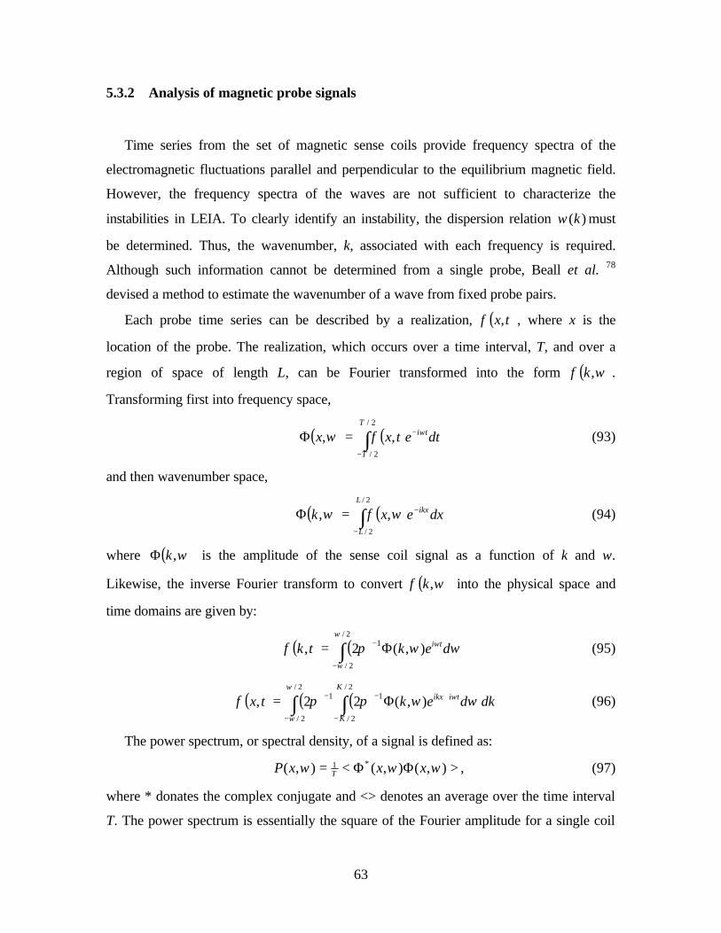
63
5.3.2 Analysis of magnetic probe signals
Time series from the set of magnetic sense coils provide frequency spectra of the
electromagnetic fluctuations parallel and perpendicular to the equilibrium magnetic field.
However, the frequency spectra of the waves are not sufficient to characterize the
instabilities in LEIA. To clearly identify an instability, the dispersion relation )(kω must
be determined. Thus, the wavenumber, k, associated with each frequency is required.
Although such information cannot be determined from a single probe, Beall et al. 78
devised a method to estimate the wavenumber of a wave from fixed probe pairs.
Each probe time series can be described by a realization, ( )tx,φ , where x is the
location of the probe. The realization, which occurs over a time interval, T, and over a
region of space of length L, can be Fourier transformed into the form ( )ωφ ,k .
Transforming first into frequency space,
( ) ( )∫−
−=Φ2/
2/
,,T
T
ti dtetxx ωφω (93)
and then wavenumber space,
( ) ( ) dxexkL
L
ikx∫−
−=Φ2/
2/
,, ωφω (94)
where ( )ω,kΦ is the amplitude of the sense coil signal as a function of k and ω.
Likewise, the inverse Fourier transform to convert ( )ωφ ,k into the physical space and
time domains are given by:
( ) ( ) ωωπφω
ω
ω dektk ti∫−
− Φ=2/
2/
1 ),(2, (95)
( ) ( ) ( )∫∫−
+−
−
− Φ=2/
2/
12/
2/
1 ),(22,K
K
tiikx dkdektx ωωππφ ωω
ω
(96)
The power spectrum, or spectral density, of a signal is defined as:
>ΦΦ<= ),(),(),( *1 ωωω xxxP T , (97)
where * donates the complex conjugate and <> denotes an average over the time interval
T. The power spectrum is essentially the square of the Fourier amplitude for a single coil
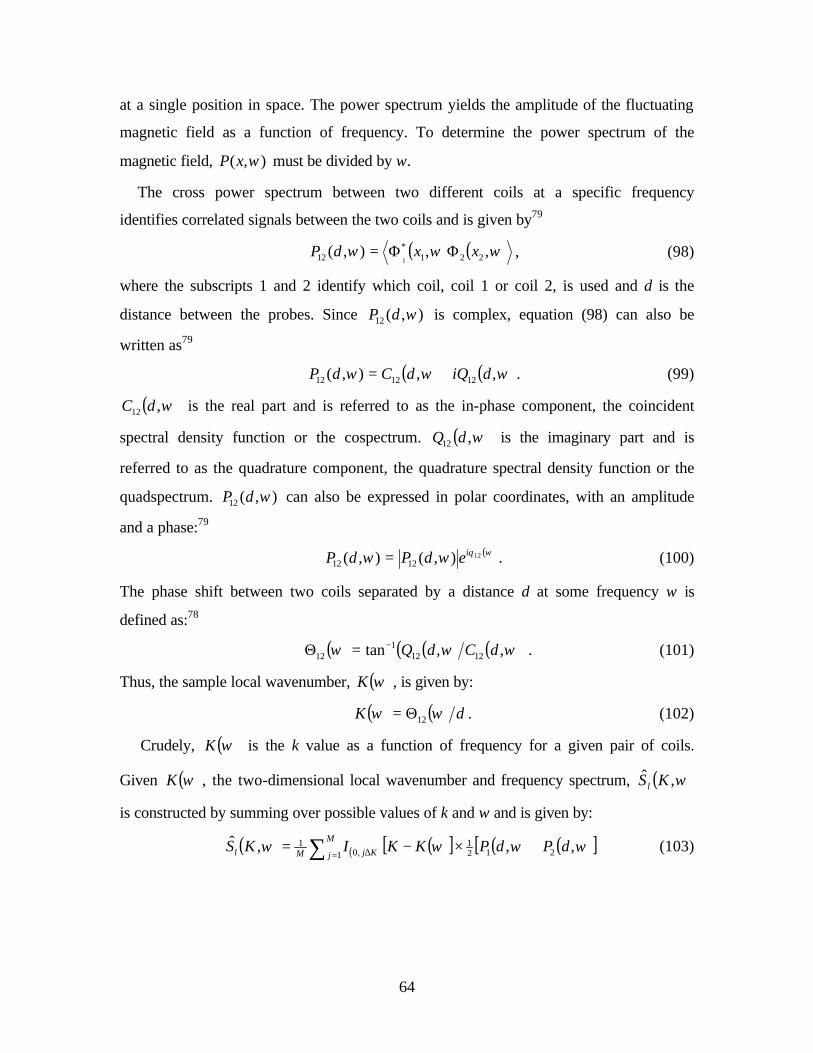
64
at a single position in space. The power spectrum yields the amplitude of the fluctuating
magnetic field as a function of frequency. To determine the power spectrum of the
magnetic field, ),( ωxP must be divided by ω.
The cross power spectrum between two different coils at a specific frequency
identifies correlated signals between the two coils and is given by79
( ) ( )ωωω ,,),( 221*
12 1xxdP ΦΦ= , (98)
where the subscripts 1 and 2 identify which coil, coil 1 or coil 2, is used and d is the
distance between the probes. Since ),(12 ωdP is complex, equation (98) can also be
written as79
( ) ( )ωωω ,,),( 121212 diQdCdP += . (99)
( )ω,12 dC is the real part and is referred to as the in-phase component, the coincident
spectral density function or the cospectrum. ( )ω,12 dQ is the imaginary part and is
referred to as the quadrature component, the quadrature spectral density function or the
quadspectrum. ),(12 ωdP can also be expressed in polar coordinates, with an amplitude
and a phase:79
( )ωθωω 12),(),( 1212iedPdP = . (100)
The phase shift between two coils separated by a distance d at some frequency ω is
defined as:78
( ) ( ) ( )( )ωωω ,,tan 12121
12 dCdQ−=Θ . (101)
Thus, the sample local wavenumber, ( )ωK , is given by:
( ) ( ) dK ωω 12Θ= . (102)
Crudely, ( )ωK is the k value as a function of frequency for a given pair of coils.
Given ( )ωK , the two-dimensional local wavenumber and frequency spectrum, ( )ω,ˆ KS l
is constructed by summing over possible values of k and ω and is given by:
( ) ( ) ( )[ ] ( ) ( )[ ]ωωωω ,,,ˆ212
11 ,0
1 dPdPKKIKSM
j KjMl +×−= ∑ = ∆ (103)

65
where ),(1 ωdP and ),(2 ωdP are the power spectra for coils 1 and coils 2 respectively; K
is the upper value of the current wavenumber bin, j∆K; and the indicator function ( )[ ]xI h,0
is defined as
( )[ ]
≤=
elsewhere
xhxI h 0
01,0 . (104)
( )ωK has a range of d2π± . ∆K, the bin size, is dM2/π , where M is the number of
points in the record and d is the distance between the two probes. For a given frequency,
( )ωK is compared to the wavenumber bin. If ( )ωK falls into the wavenumber bin, then
the average power spectra of the two coils is used to fill the bin. Otherwise, the bin is
filled with a 0. This process continues until all values of wavenumber and frequency in
the two-dimensional array are completed. A graph of ( )ω,ˆ KS l is then used to identify
peaks as a function of k and ω and the measured k and ω can then be compared to
possible dispersion relations.
To illustrate this technique, a hypothetical single frequency, traveling sine wave of
wavelength λ = 12.57 m and frequency oω = 37,700 rad/s measured by two coils a fixed
distance apart is examined (Figure 39). The single coil power spectra (Figure 40) for this
wave will be delta functions because all the power exists at a single frequency.
( ) ( )oxxP ωδω ,, 111 = (105)
( ) ( )oxxP ωδω ,, 222 = (106)
The two coils have a relative phase shift at one specific frequency, which is determined
from the cross power spectrum and equations (98) through (101). Dividing the phase shift
by the distance yields the local wavenumber at that frequency. Even though there are a
multitude of other frequencies, the local wavenumber for all those frequencies is zero in
this case because the power spectra are zero at those frequencies.
In other words, the creation of the discrete ( )ω,ˆ KSl two-dimensional array begins by
determining the local wavenumber for some particular frequency and storing the average
value of the power spectra of the two coils at that frequency. Then, the next frequency
step is examined and the process repeats until all possible ω's and k's are covered. Since
this test scenario has only a single frequency and a single wavelength, there will only be
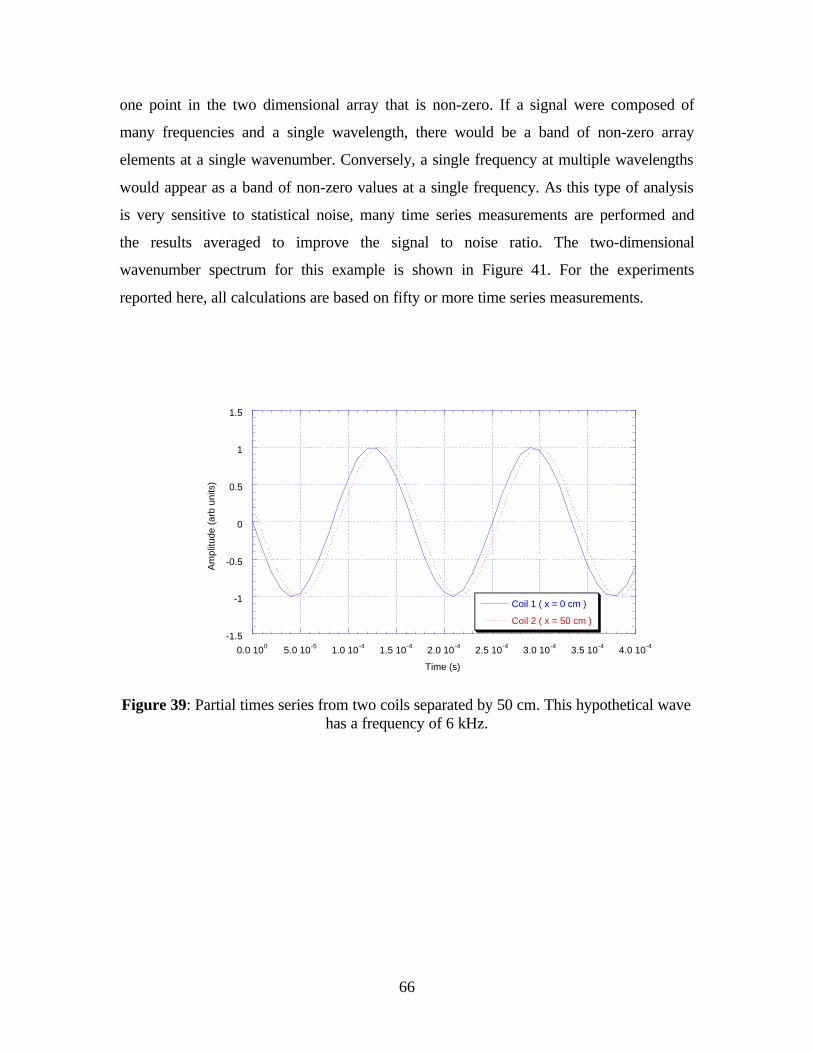
66
one point in the two dimensional array that is non-zero. If a signal were composed of
many frequencies and a single wavelength, there would be a band of non-zero array
elements at a single wavenumber. Conversely, a single frequency at multiple wavelengths
would appear as a band of non-zero values at a single frequency. As this type of analysis
is very sensitive to statistical noise, many time series measurements are performed and
the results averaged to improve the signal to noise ratio. The two-dimensional
wavenumber spectrum for this example is shown in Figure 41. For the experiments
reported here, all calculations are based on fifty or more time series measurements.
-1.5
-1
-0.5
0
0.5
1
1.5
0.0 100 5.0 10-5 1.0 10-4 1.5 10-4 2.0 10-4 2.5 10-4 3.0 10-4 3.5 10-4 4.0 10-4
Coil 1 ( x = 0 cm )
Coil 2 ( x = 50 cm )
Am
plitu
de (
arb
units
)
Time (s)
Figure 39: Partial times series from two coils separated by 50 cm. This hypothetical wave has a frequency of 6 kHz.

67
10-8
10-6
10-4
10-2
100
102
104
106
100 101 102 103 104 105
Am
plitu
de [
Hz]
2
Frequency (Hz)
Figure 40: Power spectrum of the test signal. The curve decreases with frequency because the spatial amplitude is divided by the frequency so that the amplitude of the
fluctuating quantity is found.
Figure 41: Surface plot of the wavenumber spectrum for the hypothetical case. One large peak is present at 6 kHz and k = 0.05 cm-1( λ = 12.6 m) as expected.
68
6 ELECTROMAGNETIC ION TEMPERATURE ANISOTROPY DRIVEN INSTABILITIES
Since the 1960’s, space plasma phenomena attributed to electromagnetic ion
temperature instabilities (EMITA) have been observed in the Earth's magnetosphere and
the solar wind. Vela 3 and Mariner 2 measurements of ion temperature
anisotropies80,81,82 correlated with magnetic fluctuations at frequencies below the ion
cyclotron frequency83 84, 85, 86 established a link between such anisotropies and the
excitation of electromagnetic instabilities. Analysis of these observations led to the
development of theories for the ion firehose,87 the mirror, and the ion cyclotron
anisotropy instabilities. The launch of spacecraft with more capable ion instruments in
the late 1980's, in particular the AMPTE series of spacecraft, enabled researchers to
measure three-dimensional ion distributions in both the solar wind and the
magnetosheath. Particularly in the magnetosheath, ion velocity-space distributions during
periods of enhanced low frequency electromagnetic fluctuations are observed to be bi-
Maxwellian, i.e., the ion distribution function can be represented by a Maxwellian
distribution in the direction perpendicular to the background magnetic field of one
temperature, ⊥iT , and a Maxwellian distribution function in the direction parallel to the
background magnetic field of a different temperature, ||iT . A striking feature of the
AMPTE magnetosheath data is an inverse correlation of the measured ion temperature
anisotropy, ||ii TT ⊥ , and the local plasma ion beta. Based on a combination of linear
Vlasov theory and hybrid-kinetic simulations, theorists have suggested that the inverse
correlation of ion temperature anisotropy and the local plasma beta can be explained by
the action of anisotropy driven instabilities.
Temperature anisotropies can provide a source of free energy for instability growth in
space plasmas. There are three main types of EMITA instabilities depending on the value
of the ratio of parallel and perpendicular ion temperatures. They are the ion firehose
( ⊥> TT|| ),87 the ion cyclotron87 - also called the Alfvén ion cyclotron instability
( ||TT >⊥ ),108 and the mirror instability ( ||TT >⊥ ).88,89 Each of the anisotropy driven
instabilities acts to reduce the ion temperature anisotropy. The instabilities are

69
gyroresonant with the ions and induce velocity-space diffusion that isotropizes the ion
distribution. The predicted thresholds, propagation directions, frequencies, and
wavelengths of all three instabilities are distinct. In space, both the fluctuation spectra
and propagation direction are used to identify the type of instability, given local
anisotropy measurements. The main advantages of a laboratory experiment over
spacecraft measurements are the degree of diagnostic access to the plasma, e. g., the
capability of measuring wavelengths, and varying the plasma parameters in a controlled
and reproducible fashion.
6.1 Linear Vlasov Solution
The linear growth rates of the different EMITA instabilities can be calculated using
the first-order Vlasov equation. Following the analysis of Gary91 and assuming the
primary ions in the solar wind and near-earth space environment are protons, that the
plasma is collisionless, and that the ions can be described by a bi-Maxwellian distribution
function, the collisionless Vlasov equation is:91
( ) ( ) ( ) ( )( ) ( ) 0,v,x,xBv,xE,v,xv
,v,xv =∇⋅×++∇⋅+
∂∂
tfttm
qtf
t
tfj
jj
j rrrrrrrrrrrrr, (107)
where jf is the distribution function for the jth species and the 0th order bi-Maxwellian
distribution function, ( )0jf , is:
( )( ) ( )
+−−
⊥⊥
⊥= j
j ||
2j
2y
2x
2j
2||
T
T
2v
vv
2v
v
j
j ||232
j
||0
T
T
v2v,v e
nf j
jπ
. (108)
where jv is the thermal velocity of the jth species. Linearizing and grouping the first-order
terms gives the first-order Vlasov equation:91
( )( ) ( )( ) ( )( )
( )( )( )( ) ( )( )
v
v
c
,xBv,xE
v
,v,x
c
Bv
x
,v,xv
,v,x
011
1
0
11
rrrrrrr
rrrrr
rrrrrr
∂
∂⋅
×+−
=∂
∂⋅
×+
∂∂
⋅+∂
∂
j
j
j
j
j
jjj
ftt
m
e
tf
m
etf
t
tf
(109)

70
In Cartesian geometry, equation (109) can be integrated along the unperturbed orbits to
obtain:91
( )( )( )( ) ( )( ) ( )( ) ( )ωτ
ωτ ,b1
0001 ,xE
v
vv
v
v,v,x jijj
j
jj et
fkfd
m
etf
rrr
rrr
rrrr
⋅
′∂
∂×′×+
∂
∂−= ∫ ∞−
. (110)
where
( ) ( ) ( ) ( )τωτωω
τωω
ωτ −++−= zzcjcj
yycj
cj
xyj k
kkb vsin
v1cos
v, (111)
and cmBe jojcj ≡ω is the cyclotron frequency of the jth species. The fields are assumed
to be of the form:
zBB 0=r
, (112)
( ) ( )t-x0
1 EE ωrrrr
⋅−∝ kie , (113)
( ) ( )t-x0
1 BB ωrrrr
⋅−∝ kie , (114)
and
γωω ir += . (115)
i.e., k is assumed to be real.
Typically, the dielectric tensor is calculated to determine the possible wave dispersion
relations. The dielectric tensor, Kt
, is defined as
( )( )EKEckJirtrr
⋅≡−+− 2224 ωπω . (116)
Or, in terms of the particle flux, Jerr
=Γ ,
( )( )EKEckeirtrr
⋅≡−+Γ− 2224 ωπω . (117)
However, Gary defines the dimensionless conductivity tensor, ( )ω,kS j
rt, as:
( )( ) ( ) ( )( )ωωωπ
ω ,,4
, 122
1 kEkSe
cikk j
jj
rrrtrr⋅−=Γ . (118)
and rewrites the perturbed flux, ( ) ( )ω,1 kj
rrΓ , in terms of the perturbed distribution function
to solve for the allowed dispersion relations. For 0B =×rr
k , which applies to the firehose
and ion cyclotron anisotropy instabilities, equation (110) is substituted into equation
(118). After considerable algebra, equation (118) yields:
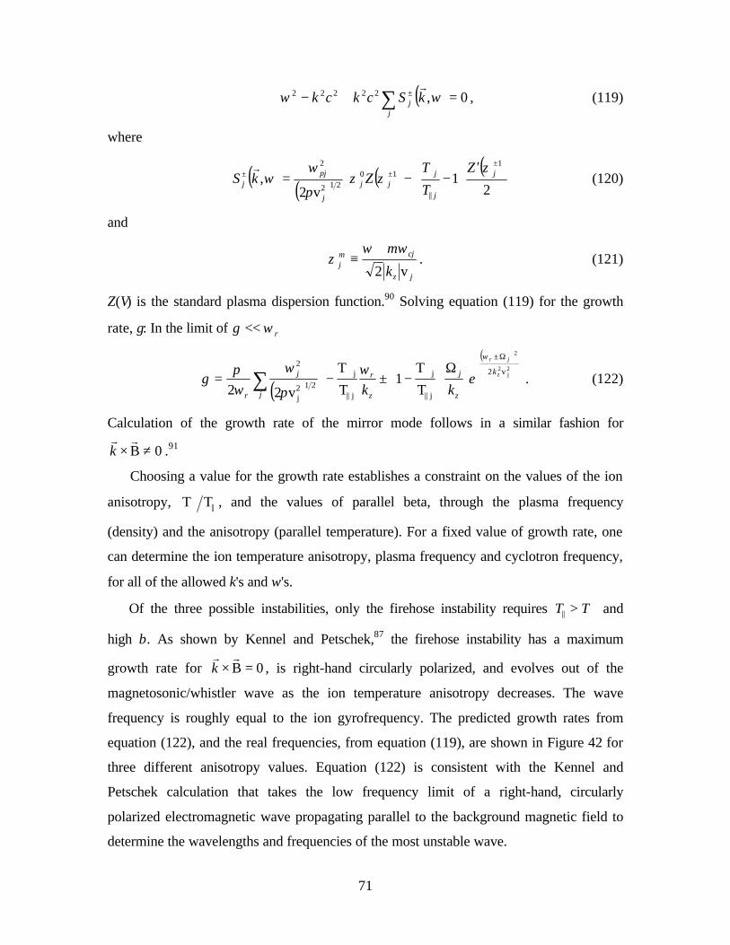
71
( )∑ =+− ±
jj kSckck 0,22222 ωω
r, (119)
where
( ) ( ) ( ) ( )
′
−−=
±⊥±±
21
v2,
1
||
10212
2j
j
jjj
j
pjj
Z
T
TZkS
ζζζ
π
ωω
r (120)
and
jz
cjmj
k
m
v2
ωωζ
+≡ . (121)
Z(ς) is the standard plasma dispersion function.90 Solving equation (119) for the growth
rate, γ: In the limit of rωγ <<
( )
( )
Ω±
⊥⊥∑
Ω
−±−=
2j
2
2
v2
j ||
j
j ||
j
212j
2
T
T1
T
T
v22z
jr
k
j z
j
z
rj
r
ekk
ω
ω
π
ω
ωπ
γ . (122)
Calculation of the growth rate of the mirror mode follows in a similar fashion for
0B ≠×rr
k .91
Choosing a value for the growth rate establishes a constraint on the values of the ion
anisotropy, ||TT⊥ , and the values of parallel beta, through the plasma frequency
(density) and the anisotropy (parallel temperature). For a fixed value of growth rate, one
can determine the ion temperature anisotropy, plasma frequency and cyclotron frequency,
for all of the allowed k's and ω's.
Of the three possible instabilities, only the firehose instability requires ⊥> TT|| and
high β. As shown by Kennel and Petschek,87 the firehose instability has a maximum
growth rate for 0B =×rr
k , is right-hand circularly polarized, and evolves out of the
magnetosonic/whistler wave as the ion temperature anisotropy decreases. The wave
frequency is roughly equal to the ion gyrofrequency. The predicted growth rates from
equation (122), and the real frequencies, from equation (119), are shown in Figure 42 for
three different anisotropy values. Equation (122) is consistent with the Kennel and
Petschek calculation that takes the low frequency limit of a right-hand, circularly
polarized electromagnetic wave propagating parallel to the background magnetic field to
determine the wavelengths and frequencies of the most unstable wave.

72
Figure 42: The real frequency (solid line) and growth rates (dots) for the ion firehose instability for three different ion temperature anisotropies. Both the real frequency ( rω )
and the growth rate (γ ) are normalized with respect to the ion cyclotron frequency ( iΩ ).
The plasma parameters used in the calculation were pe TT = , 410v −=calfven , and 2=β . 91
Although the ion cyclotron anisotropy and the mirror instabilities occur over roughly
the same values of ion beta, they are distinctly different. The ion cyclotron anisotropy
instability has a lower anisotropy threshold than the mirror instability for low values of
beta ( 6<β ).92 In a stationary, homogenous plasma, the mirror mode has zero real
frequency, which means it is a DC signal. The ion cyclotron anisotropy instability occurs
at frequencies lower then the ion cyclotron frequency, usually in the range of
( cici ωω 8.02.0 − ). At low values of beta, the ion cyclotron anisotropy instability is
predicted to dominate over the mirror instability. However, simulations have shown that a
small helium-ion component can reduce the linear growth rate of the proton cyclotron
instability without significantly affecting the mirror instability.93 Future experiments in
LEIA using two different ion species could be performed to observe the changes in the
ion cyclotron anisotropy instability as a function of heavier ion concentration. At high
values of β ( 6>β ) the mirror mode has a lower anisotropy threshold.92
The ion cyclotron anisotropy instability is characterized by primarily transverse
fluctuations, while the mirror fluctuations are compressional for 1<β . The growth rates

73
for three different values of ion temperature anisotropies for the ion cyclotron anisotropy
instability are shown in Figure 43. The growth rates of the mirror instability for three ion
temperature anisotropies are shown in Figure 44. The results shown in Figure 43 can be
compared to the calculations by Davidson and Ogden94 for similar parameters (Figure
45). Davidson and Ogden solved the dispersion relation in the limit of 0|| =iT .
( ) 02
2222
212222 =
±−
±−− ⊥
ci
cizi
cipi
cepe kckc
ωωω
βωω
ωω
ωω
ω∓ . (123)
In the 0|| =iT limit, the ||iT terms cancel in the dispersion relation. As seen in Figure 43,
the parallel wavenumber of the fastest growing mode increases with increasing
ansotropy, consistent with equation (123).
Figure 43: The real frequency (solid line) and growth rate (dots) for the ion-cyclotron instability for three different ion temperature anisotropies. 1=β . 91
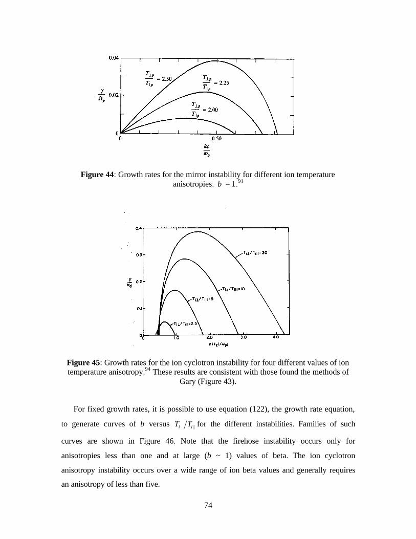
74
Figure 44: Growth rates for the mirror instability for different ion temperature anisotropies. 1=β .91
Figure 45: Growth rates for the ion cyclotron instability for four different values of ion temperature anisotropy.94 These results are consistent with those found the methods of
Gary (Figure 43).
For fixed growth rates, it is possible to use equation (122), the growth rate equation,
to generate curves of β versus ||ii TT ⊥ for the different instabilities. Families of such
curves are shown in Figure 46. Note that the firehose instability occurs only for
anisotropies less than one and at large (β ~ 1) values of beta. The ion cyclotron
anisotropy instability occurs over a wide range of ion beta values and generally requires
an anisotropy of less than five.

75
Figure 46: Beta versus Anisotropy inverse correlation for the three different instabilities for different growth rates. The solid lines to the left of an anisotropy of unity correspond
to the ion firehose instability. The solid lines to the right of an anisotropy of unity correspond to the ion cyclotron instability. The dashed lines correspond to the MHD
thresholds for the non-resonant firehose and mirror instabilities.91
In addition to analytic investigations, both the mirror and ion cyclotron anisotropy
instabilities have been the subject of numerous computational studies. Most of the studies
have used the 1-D hybrid code developed by Winske and Omidi.95 A hybrid code treats
the electrons as a massless fluid and treats the ions as discrete marcroparticles. This
treatment allows calculations to be done on the ion time scale instead of the electron time
scale, thereby focusing on the ion physics exclusively. The computations include all three
components of the ion velocities, the currents and the electric and magnetic fields. To
model bi-Maxwellian effects in a 1-D code, two ion components are used: a cold ion
background and a beam drifting with respect to the cold component along the background

76
magnetic field. All of the calculations are performed in the rest frame of the electrons,
where the ion current is zero. In the one-dimensional calculations, the x coordinate is the
direction of k. In the two-dimensional codes, the magnetic field is along the x-coordinate
and the waves develop in the x-y plane. Other researchers have studied the expected wave
spectra using 2-D hybrid codes.96
Recently, driven simulations have been reported in literature.97 In driven simulations,
the ions’ velocities are periodically altered to increase the ion temperature anisotropy.
This method is done to simulate a driving mechanism that keeps the ion's anisotropy near
the value needed to excite the EMITA instability, similar to the conditions believed to
exist in the magnetosheath. Many of the spacecraft observations occur in a region of
space called the plasma depletion layer (PDL). Plasma constantly enters the PDL from
the magnetosheath proper with a higher ion temperature anisotropy than in the PDL.
Even though the anisotropy begins to decrease in the PDL, there is a constant supply of
ions with large enough anisotropies to maintain a large, steady, ion temperature
anisotropy.
Besides predicting the growth rates and wavenumbers for the various instabilities,
Gary also noticed that a fixed value of the maximum growth rate of the ion cyclotron
anisotropy instability leads to an inverse correlation between the ion temperature
anisotropy and the ion parallel beta. The correlation is of the form
αβ||||
1S
T
T=−⊥ , (124)
where S is dimensionless and depends on the choice of maximum growth rate and the
density of the hot protons and 5.0≈α . Fit parameters based on equation (124) for
various theoretical studies are tabulated in Table 6 for the ion temperature instability.
The choice of a particular value of maximum growth rate is predicated on the
assumption that once such a value of growth rate is reached, the amplitude of the
instability becomes large enough to induce strong velocity-space diffusion and thereby
supresses the ion temperature anisotropy, i.e., a self-limiting process as described by
Manheimer and Boris.1 Note that it is the maximum growth rate, regardless of the
particular ω and k of the instability, that is held fixed. As the ion temperature anisotropy
and parallel ion beta change, the wavenumber and frequency associated with the

77
maximum growth rate also change. However, the assumption here is that when the
growth rate of the instability reaches some maximum value, the growth rate can increase
no further.
For values of ion temperature anisotropy and parallel ion beta that lie below the
maximum growth rate curve, fluctuations driven by the anisotropy can exist and grow in
amplitude, but at a rate less than the maximum growth rate. As the value of beta
increases, very little anisotropy is required to reach the maximum growth rate. Thus, at
high values of beta, only modest values of ion temperature anisotropy can exist. If, at a
fixed value of beta, the value of anisotropy were increased, the growth rate of the
instability would increase until the maximum value was reached. At that point,
equilibrium between fluctuation growth rate and velocity space diffusion would be
reached and the anisotropy could not be increased any further. When collisions are
considered, there is a little change in the above picture. "It is expected that collisions will
result in fewer anisotropy measurements near the maximum growth rate curve. Relatively
more anisotropy measurements will lie below the maximum growth rate curve,
representing cases in which collisions have had time to further the anisotropy."98 The
approach used in Gary's calculations is linear and therefore the maximum growth rate
calculations are based purely on linear theory. The interpretation of the balance between
the wave's growth due to finite anisotropy and the scattering in velocity-space due to the
fluctuation amplitude resembles a quasi-linear interpretation.
Table 6: Fit parameters for the ion temperature anisotropy - beta inverse correlation for different simulations and growth rates in the linear Vlasov model.
Gary Model S αα
1-D Hybrid: Driven Case97 0.55 0.52
Linear Vlasov - ( )pΩ= −410γ 97 0.35 0.42
Linear Vlasov – ( )pΩ= −310γ 97 0.43 0.42
Linear Vlasov – ( )pΩ= −210γ 97 0.65 0.40
Linear Vlasov – Ion Cyclotron99 0.66 0.40
Linear Vlasov – Mirror99 0.97 0.61

78
6.2 Recent Spacecraft Observations
Researchers using data from the Active Magnetosphere Particle Tracer Explorers
(AMPTE) Charge Composition Explorer (CCE) spacecraft, the APMTE Ion Release
Module (IRM), and the WIND spacecraft have all reported the existence of an upper
bound on the ion temperature anisotropy versus ion beta in the Earth's magnetosheath.
Wave activity around the cyclotron frequency was often, but not always observed in
conjunction with large ion temperature anisotropies.
Though they were part of the same mission, there are significant differences between
the CCE and IRM spacecraft. The apogee of AMPTE/CCE was 8.8 ER (Earth radii) and
the apogee of IRM was 18.8 ER . Each spacecraft was equipped with magnetometers to
measure the three dimensional magnetic field fluctuations. AMPTE/IRM measured the
energy distribution of ions with a three-dimensional (spin and azimuthal) electrostatic
analyzer. However, the AMPTE/CCE plasma instrument was a simple two-dimensional
electrostatic analyzer (spin only). The AMPTE/CCE ion temperature anisotropy
measurements were sensitive to variations in the direction of the magnetic field as the
instrument lacked resolution out of the spin plane of the spacecraft.100 Thus, it is likely
that the AMPTE/CCE ion temperature measurements over-estimate the level of ion
temperature anisotropy in the magnetosheath.101
The AMPTE spacecraft data relevant to this investigation were taken in the
magnetosheath and across the magnetopause (see Figure 47). Near the magnetopause,
magnetosheath flow can give rise to a region of decreased plasma density and increased
magnetic field strength,4 i.e. lower beta. This region is called a plasma depletion layer
(PDL). When a PDL is formed, the plasma and field in it are representative of the
magnetopause and not the magnetosheath. Since the PDL typically has a lower beta than
the magnetosheath, the mirror instability is not as likely to be present in the PDL and care
must be used in comparing PDL and magnetosheath measurements.102

79
Figure 47: Location of magnetosheath and magnetopause. The PDL occurs on the sunward side of the magnetopause.91
Anderson et al. reported a study of ion temperature anisotropies in the magnetosheath
and the plasma depletion layer using AMPTE/CCE data.103 They limited their study only
to events where magnetic fluctuations were also observed. Data from Anderson et al.103
are shown in Figure 48. The data are grouped by the local plasma environment. In high β
- low A environments, where 1|| −≡ ⊥ TTA , the fluctuations are compressional, while in
low β - high A environments the waves are transverse. In each case, a least-squares fit of
the form αβSA −= 1 is performed for the ion anisotropy versus parallel ion beta data.

80
Figure 48: Anderson's data from the AMPTE/CCE spacecraft. Bifurcated data are correlated with observations of transverse waves with two broad maxima in the frequency
spectra. Data classified as continuous had transverse waves with continuous power spectra extending above and below half the proton cyclotron frequency. Low/Transverse data consisted of data with transverse waves below half the proton cyclotron frequency.
Data classified as low/transverse and mirror consists of intervals with a prominent compressional peak and a transverse peak, below half the proton cyclotron frequency, at different frequencies. Mirror data is dominated by compressional perturbations with no
discernible transverse peak.103
The AMPTE/CCE data indicate that during periods of low frequency wave activity,
there is an inverse correlation between the upper bound on the temperature anisotropy of
the ions and the parallel ion beta. The frequency spectra of the waves were also compared
to the predictions of linear Vlasov theory. The observed transverse wave spectra were in
good agreement with the theoretical predictions for the ion cyclotron wave, while the
observed compressional spectral structures were in good agreement with the predictions
for the mirror mode.103 The mirror mode-like waves were observed when the spacecraft
was in the magnetosheath proper (high β), while the ion cyclotron-like waves were
observed when the spacecraft was in the PDL (low β).
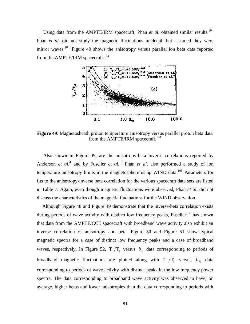
81
Using data from the AMPTE/IRM spacecraft, Phan et al. obtained similar results.104
Phan et al. did not study the magnetic fluctuations in detail, but assumed they were
mirror waves.104 Figure 49 shows the anisotropy versus parallel ion beta data reported
from the AMPTE/IRM spacecraft.104
Figure 49: Magnetosheath proton temperature anisotropy versus parallel proton beta data from the AMPTE/IRM spacecraft.104
Also shown in Figure 49, are the anisotropy-beta inverse correlations reported by
Anderson et al.4 and by Fuselier et al..6 Phan et al. also performed a study of ion
temperature anisotropy limits in the magnetosphere using WIND data.105 Parameters for
fits to the anisotropy-inverse beta correlation for the various spacecraft data sets are listed
in Table 7. Again, even though magnetic fluctuations were observed, Phan et al. did not
discuss the characteristics of the magnetic fluctuations for the WIND observation.
Although Figure 48 and Figure 49 demonstrate that the inverse-beta correlation exists
during periods of wave activity with distinct low frequency peaks, Fuselier106 has shown
that data from the AMPTE/CCE spacecraft with broadband wave activity also exhibit an
inverse correlation of anisotropy and beta. Figure 50 and Figure 51 show typical
magnetic spectra for a case of distinct low frequency peaks and a case of broadband
waves, respectively. In Figure 52, ||TT⊥ versus ||iβ data corresponding to periods of
broadband magnetic fluctuations are plotted along with ||TT⊥ versus ||iβ data
corresponding to periods of wave activity with distinct peaks in the low frequency power
spectra. The data corresponding to broadband wave activity was observed to have, on
average, higher betas and lower anisotropies than the data corresponding to periods with
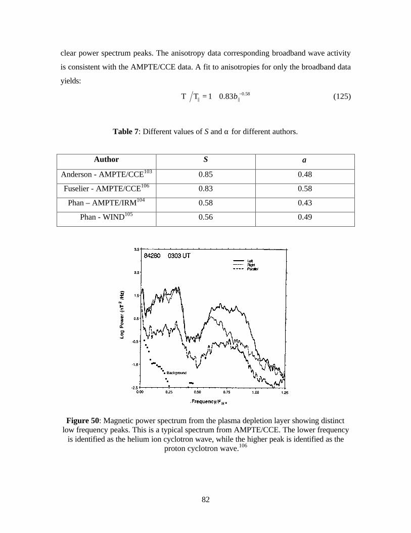
82
clear power spectrum peaks. The anisotropy data corresponding broadband wave activity
is consistent with the AMPTE/CCE data. A fit to anisotropies for only the broadband data
yields:
58.0|||| 83.01TT −
⊥ += β (125)
Table 7: Different values of S and α for different authors.
Author S αα
Anderson - AMPTE/CCE103 0.85 0.48
Fuselier - AMPTE/CCE106 0.83 0.58
Phan – AMPTE/IRM104 0.58 0.43
Phan - WIND105 0.56 0.49
Figure 50: Magnetic power spectrum from the plasma depletion layer showing distinct low frequency peaks. This is a typical spectrum from AMPTE/CCE. The lower frequency
is identified as the helium ion cyclotron wave, while the higher peak is identified as the proton cyclotron wave.106
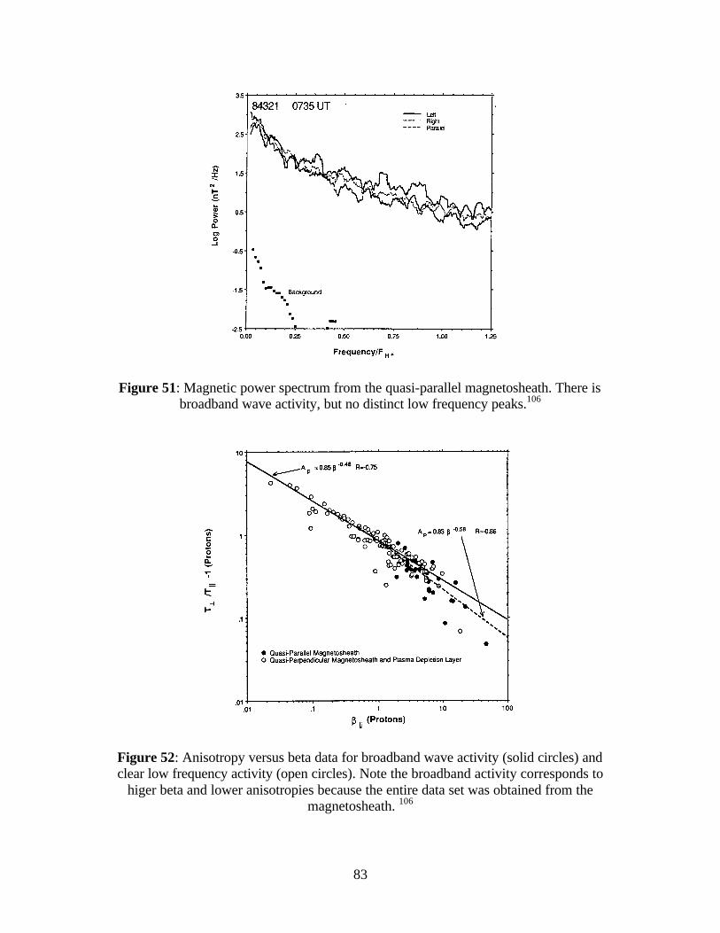
83
Figure 51: Magnetic power spectrum from the quasi-parallel magnetosheath. There is broadband wave activity, but no distinct low frequency peaks.106
Figure 52: Anisotropy versus beta data for broadband wave activity (solid circles) and clear low frequency activity (open circles). Note the broadband activity corresponds to
higer beta and lower anisotropies because the entire data set was obtained from the magnetosheath. 106

84
6.3 Previous Experimental Investigations of EMITA Instabilities
Alfvén ion cyclotron instabilities (AIC), or ion cyclotron anisotropy instabilities, have
been observed before in the laboratory. Experiments in both the tandem mirror machine,
GAMMA 10107 and the Tandem Mirror experiment (TMX) 108 observed AIC waves along
with ||TT >⊥ anisotropies. Casper and Smith presented the first experimental evidence for
the presence of the Alfvén ion cyclotron (AIC) instability through measurements of
magnetic fluctuations just below the hydrogen cyclotron frequency and indirect
measurements of the temperature anisotropy.108 Their values of ⊥iβ and ⊥iβ A2 exceeded
the Davidson and Ogden theoretical threshold ( )5.3A2 ≥⊥iβ for the AIC instability.109
Here ||TTA ⊥= . Thus, they concluded the observed transverse right circularly polarized
waves must be AIC waves. Similar results were also obtained from GAMMA 10,110, 111
though their values of ⊥iβ A2 were much lower than the theoretical
threshold ( )3.0A2 ≥⊥iβ (Figure 53). The most compelling aspect of those experiments
was the observation that the AIC waves only appeared above a ⊥iβ A2 threshold.
However, there was no indication of an upper bound on the ion temperature anisotropy
even though relatively large betas were achieved. Figure 54 compares the ⊥iβ A2
threshold observed by the GAMMA 10 group to the space data and theory curves
discussed previously. A key difference between the GAMMA 10 results and the
spacecraft measurements is the range of ⊥iβ . Although large values of ⊥iβ were obtained,
||iβ may not have been large enough to keep the plasma near the instability threshold seen
in space and in theory.

85
Figure 53: Results from the GAMMA 10 experiment.110 The dashed line is the theoretical curve for ( )5.3A2 ≥⊥β . The solid curves are for different growth rates for the AIC instability. The solid circles represent measurements when wave activity was present
and the open circles when wave activity was not present. There is no apparent upper bound on the anisotropy as there is in the spacecraft data.110
0.1
1
10
100
0.0001 0.001 0.01 0.1 1 10
Gary - Driven Case
Gary - .01ωci growth rate
Phan Results
Anderson Results
Gamma 10 experimental results
Ani
sotr
opy
(T⊥/T
||)
Parallel Ion Beta
Figure 54: The GAMMA 10 observed instability threshold compared to other computation models and spacecraft results.
86
7 EXPERIMENTAL RESULTS ON ION TEMPERATURE ANISOTROPY UPPER BOUND
As part of this investigation into EMITA instabilities, two different experiments were
performed. The first was designed to determine if an inverse correlation between the ion
temperature anisotropy and the parallel ion beta exists in LEIA plasmas. The second was
designed to determine if ion temperature anisotropy reduction could be directly
associated with low frequency electromagnetic waves. In section 7.1, all of the LEIA
measurements are compared to the theory calculations and space observations. Section
7.2 examines the role collisions play in limiting the ion temperature anisotropy. Section
7.3 reviews evidence concerning the role low frequency electromagnetic waves play in
the reduction of anisotropy between two axial positions in LEIA. The collisionality of the
laboratory plasma is a significant effect and is one of the limitations of laboratory
modeling of space plasmas. Magnetosheath plasmas are collisionless ( )1>>Lmfpλ while
the experiment is marginally collisional ( )1~Lmfpλ : mfpλ is the ion mean free path and L
is the system scale size. The experiments also have a boundary (the vacuum chamber),
which is not present in space, and use a heavier ion species, argon instead of hydrogen. In
addition, the experiment only uses one species of ions instead of two, which is commonly
observed in the magnetosheath (hydrogen and helium). Finally, the ratio of the electron
temperature to the ion temperature is much higher in the experiment (5 - 10) than in the
simulations91 or in the magnetosheath.4
7.1 Inverse Correlations of ||ii TT ⊥ and ||iβ
Previous experiments demonstrated that an intrinsic ion temperature anisotropy exists
in HELIX.112 The anisotropy persists as the plasma expands from HELIX into LEIA and
supplies an initial anisotropy that can drive instabilities in LEIA. This situation is
analogous to the driven case that has been studied computationally and in the in-situ PDL
data.
Ion temperature anisotropies in LEIA were measured over a wide range of plasma
conditions. Every experiment was performed using argon gas at a HELIX fill pressure of

87
1.8 mTorr. The HELIX magnetic field ranged from 399 G to 1264 G and the LEIA
magnetic field ranged from 18 G to 70 G. An 8 MHz rf driving signal, at a power of
400 W, was used to drive a 19 cm right helical antenna to generate the plasma in HELIX.
For each experimental configuration, both the ion temperature anisotropy and the plasma
beta were measured. The ion temperatures were measured both upstream (re-entrant
probe) and downstream (radial probe). The beta was calculated based on Langmuir probe
density measurements at both axial positions and the vacuum magnetic field. Plotted on a
log-log scale in Figure 55 and a linear scale in Figure 56 are the average anisotropies
versus average parallel ion beta. The averaged quantities were calculated from the
average of a series of ion temperature measurements for a given experimental
configuration. To estimate the error in the average measurements, "super-averaged" data
values were also calculated. The "super-averaged" data are obtained by averaging the
average anisotropies and average betas for similar experimental configurations used on
different days. The "super-averaged" data are plotted with averaged data, along with the
standard deviations from each "super averaged" data set. The deviations of the ion
temperature anisotropy and parallel ion beta were typically 10 - 20 %. Figure 55 and
Figure 56 include both upstream and downstream measurements. The data stretches over
roughly two orders of magnitude in beta and one order of magnitude in ion temperature
anisotropy. The data exhibit a clear upper bound on the anisotropy level that is in good
agreement with both extrapolation of the AMPTE/IRM results and simulations of the ion
cyclotron anisotropy instability. The data best fit the ion cyclotron anisotropy instability
simulations that used ciωγ 310−= . Therefore, this simulation result was chosen to
compare to the data. In order to compare the data to the spacecraft measurements, the fits
to the spacecraft data were extrapolated to include the range of betas spanned in the
experiment. Low frequency fluctuations are present in nearly all of the data.
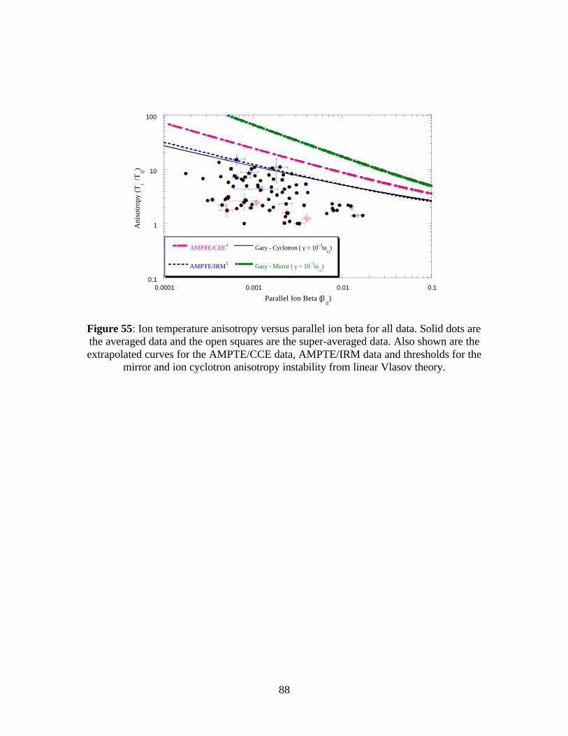
88
0.1
1
10
100
0.0001 0.001 0.01 0.1
AMPTE/CEE4
AMPTE/IRM5
Gary - Cyclotron ( γ = 10-3ωci)
Gary - Mirror ( γ = 10 -3ωci)
Ani
sotr
opy
(Ti⊥
/Ti||)
Parallel Ion Beta (βι||)
Figure 55: Ion temperature anisotropy versus parallel ion beta for all data. Solid dots are the averaged data and the open squares are the super-averaged data. Also shown are the extrapolated curves for the AMPTE/CCE data, AMPTE/IRM data and thresholds for the
mirror and ion cyclotron anisotropy instability from linear Vlasov theory.
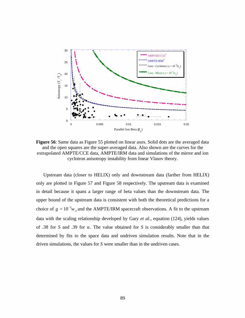
89
0
5
10
15
20
25
30
0 0.005 0.01 0.015 0.02
AMPTEE/CCE4
AMPTE/IRM5
Gary - Cyclotron ( γ = 10 -3ωci)
Gary - Mirror ( γ = 10 -3ωci)
Ani
sotr
opy
(Ti⊥
/Ti||)
Parallel Ion Beta (βi||)
Figure 56: Same data as Figure 55 plotted on linear axes. Solid dots are the averaged data and the open squares are the super-averaged data. Also shown are the curves for the
extrapolated AMPTE/CCE data, AMPTE/IRM data and simulations of the mirror and ion cyclotron anisotropy instability from linear Vlasov theory.
Upstream data (closer to HELIX) only and downstream data (farther from HELIX)
only are plotted in Figure 57 and Figure 58 respectively. The upstream data is examined
in detail because it spans a larger range of beta values than the downstream data. The
upper bound of the upstream data is consistent with both the theoretical predictions for a
choice of ciωγ 310−= and the AMPTE/IRM spacecraft observations. A fit to the upstream
data with the scaling relationship developed by Gary et al., equation (124), yields values
of .38 for S and .39 for α. The value obtained for S is considerably smaller than that
determined by fits to the space data and undriven simulation results. Note that in the
driven simulations, the values for S were smaller than in the undriven cases.
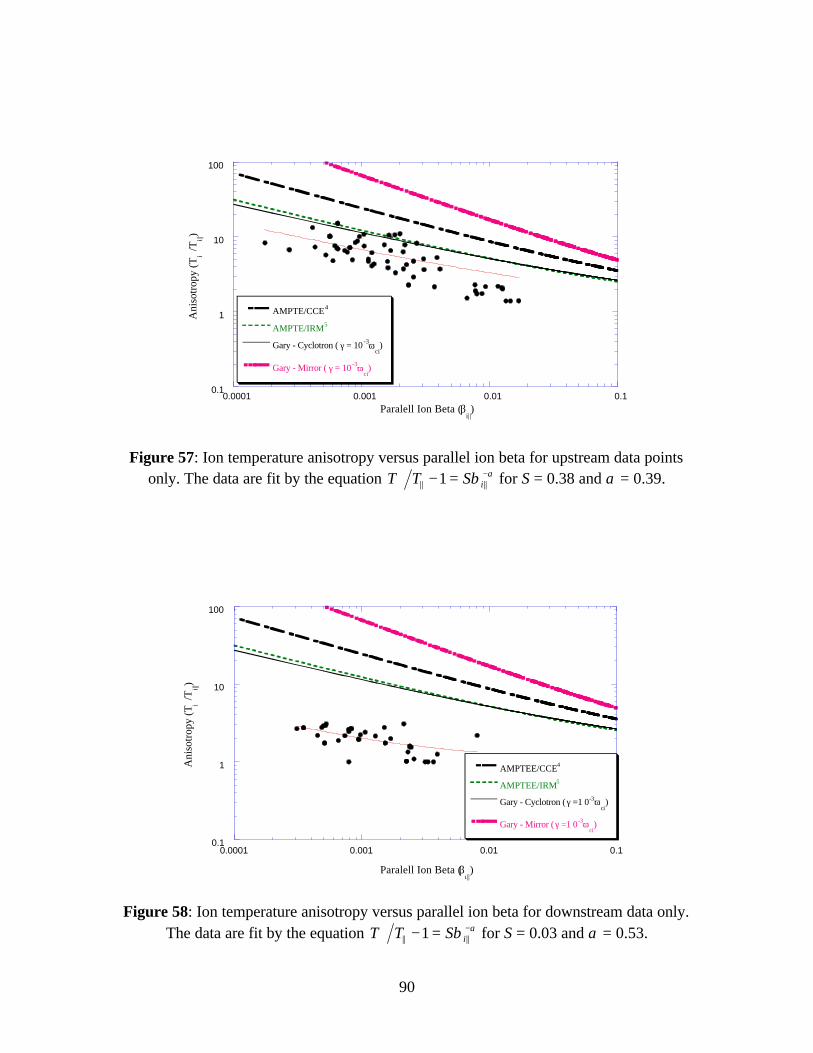
90
0.1
1
10
100
0.0001 0.001 0.01 0.1
AMPTE/CCE4
AMPTE/IRM5
Gary - Cyclotron ( γ = 10 -3ωci)
Gary - Mirror ( γ = 10 -3ωci)
Ani
sotr
opy
(Ti ⊥
/Ti||)
Paralell Ion Beta (βi||)
Figure 57: Ion temperature anisotropy versus parallel ion beta for upstream data points only. The data are fit by the equation αβ −
⊥ =− |||| 1 iSTT for S = 0.38 and α = 0.39.
0.1
1
10
100
0.0001 0.001 0.01 0.1
AMPTEE/CCE4
AMPTEE/IRM5
Gary - Cyclotron (γ =1 0-3ωci)
Gary - Mirror (γ =1 0-3ωci)
Ani
sotr
opy
(Ti⊥
/Ti||)
Paralell Ion Beta (βι||)
Figure 58: Ion temperature anisotropy versus parallel ion beta for downstream data only. The data are fit by the equation αβ −
⊥ =− |||| 1 iSTT for S = 0.03 and α = 0.53.

91
A fit of the scaling relationship to the downstream data yields values of .03 for S and
.53 for α. The value of S is much smaller than for the upstream data. Note that the
anisotropy values are considerably smaller in the downstream data versus the upstream
data. The ion temperature anisotropy is reduced by collisions, discussed in more detail in
the next section, and perhaps by the wave-particle interactions of an instability. As the
plasma flows towards the downstream measurement location where the anisotropy is
smaller, any anisotropy driven instabilities should shrink in amplitude and growth rate.
Thus, it is unlikely that downstream measurements are representative of a strongly driven
system near an anisotropy instability threshold.
7.2 Collisions
Unlike the magnetosphere, where plasma densities are extremely small and the plasma
is essentially collisionless, these experiments are performed in a marginally collisional
plasma. To compare these results to collisionless theory, the effect of varying collision
frequencies must be eliminated. Collisions tend to isotropize a plasma by transferring
energy from one direction to the another, i.e. velocity space diffusion. Experimentally,
the effects of collisions cannot be eliminated but the effects of variations in the
collisionality can be minimized by varying the ion temperature anisotropy and parallel
ion beta while keeping the relevant collision rates fixed.
Ignoring ion-electron collisions, the rates of change for the perpendicular and parallel
temperatures are given by113
( )||||
2
1TT
dt
dT
dt
dT−−=−= ⊥
⊥ ν , (126)
where
( ) ( ) ( )
++−≈
−
A
AA
AkTm
ne
i
1
223||
4 tan33
22 πν , (127)
1||
−≡ ⊥
T
TA . (128)
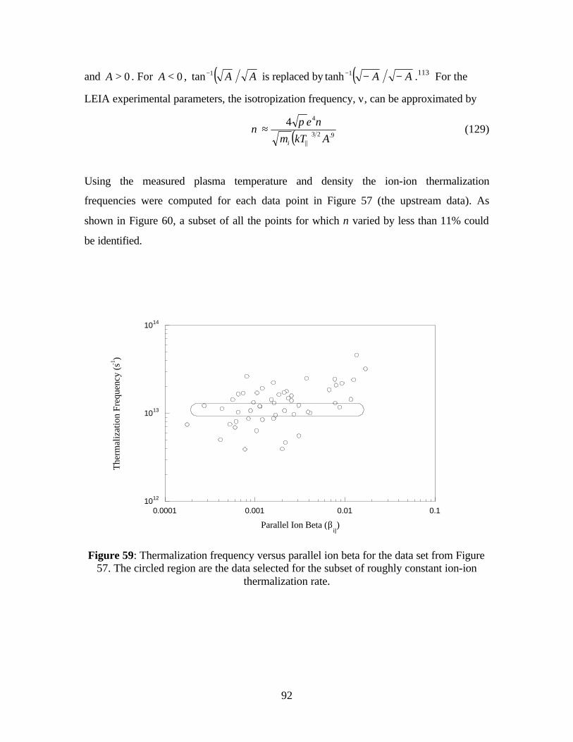
92
and 0>A . For 0<A , ( ) AA1tan− is replaced by ( ) AA −−−1tanh .113 For the
LEIA experimental parameters, the isotropization frequency, ν, can be approximated by
( ) 9.23||
44
AkTm
ne
i
πν ≈ (129)
Using the measured plasma temperature and density the ion-ion thermalization
frequencies were computed for each data point in Figure 57 (the upstream data). As
shown in Figure 60, a subset of all the points for which ν varied by less than 11% could
be identified.
1012
1013
1014
0.0001 0.001 0.01 0.1
The
rmal
izat
ion
Freq
uenc
y (s
-1)
Parallel Ion Beta (βi||)
Figure 59: Thermalization frequency versus parallel ion beta for the data set from Figure 57. The circled region are the data selected for the subset of roughly constant ion-ion
thermalization rate.

93
0.01
0.1
1
10
100
0.0001 0.001 0.01 0.1
AMPTE/IRM5
AMPTE/CCE4
Gary - Cyclotron (γ = 10-3 ωci)
Ani
sotr
opy
(Ti ⊥
/Ti||)
Parallel Ion Beta ( βi||)
Figure 60: Anisotropy versus beta for a subset of the data with similar ion-ion thermalization frequencies.
The anisotropy versus beta data for the subset of data with similar ion-ion
thermalization rates is shown in Figure 63. It is worth noting that if ion-ion collisions
were the only source of isotropization, the anisotropy would scale more strongly than
1||−iβ since both the collision frequency and βi|| increase linearly with increasing density.
The data extend over an order of magnitude in beta and a factor of roughly five in
anisotropy. The trend remains consistent with the space measurements and theoretical
predictions. To eliminate the effects of variation in ion-neutral collisionality, only those
data for which the ion-neutral collision frequencies were the same were identified. For
ease of analysis, a constant ion-neutral cross section was assumed. For a total energy of
0.4 eV to 1.7 eV, such an approximation is reasonable (see Figure 61). Thus, the ion-
neutral collision frequency is proportional to iT , where ( ) 32 2||
22iii TTT += ⊥ . Figure 62
shows the ion-neutral collision frequencies versus βi|| for the data of Figure 60. Again, a
subset varying by less than 11% can be identified. Even though this highly constrained
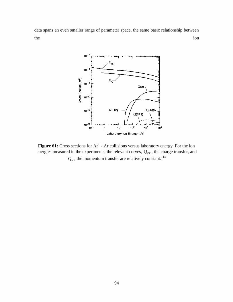
94
data spans an even smaller range of parameter space, the same basic relationship between
the ion
Figure 61: Cross sections for Ar+ - Ar collisions versus laboratory energy. For the ion energies measured in the experiments, the relevant curves, CTQ , the charge transfer, and
mQ , the momentum transfer are relatively constant.114
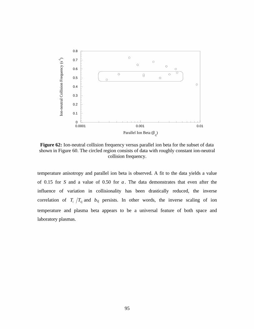
95
0
0.1
0.2
0.3
0.4
0.5
0.6
0.7
0.8
0.0001 0.001 0.01
Ion-
neut
ral C
ollis
ion
Freq
uenc
y (s
-1)
Parallel Ion Beta (βi||)
Figure 62: Ion-neutral collision frequency versus parallel ion beta for the subset of data shown in Figure 60. The circled region consists of data with roughly constant ion-neutral
collision frequency.
temperature anisotropy and parallel ion beta is observed. A fit to the data yields a value
of 0.15 for S and a value of 0.50 for α. The data demonstrates that even after the
influence of variation in collisionality has been drastically reduced, the inverse
correlation of ||ii TT ⊥ and βi|| persists. In other words, the inverse scaling of ion
temperature and plasma beta appears to be a universal feature of both space and
laboratory plasmas.
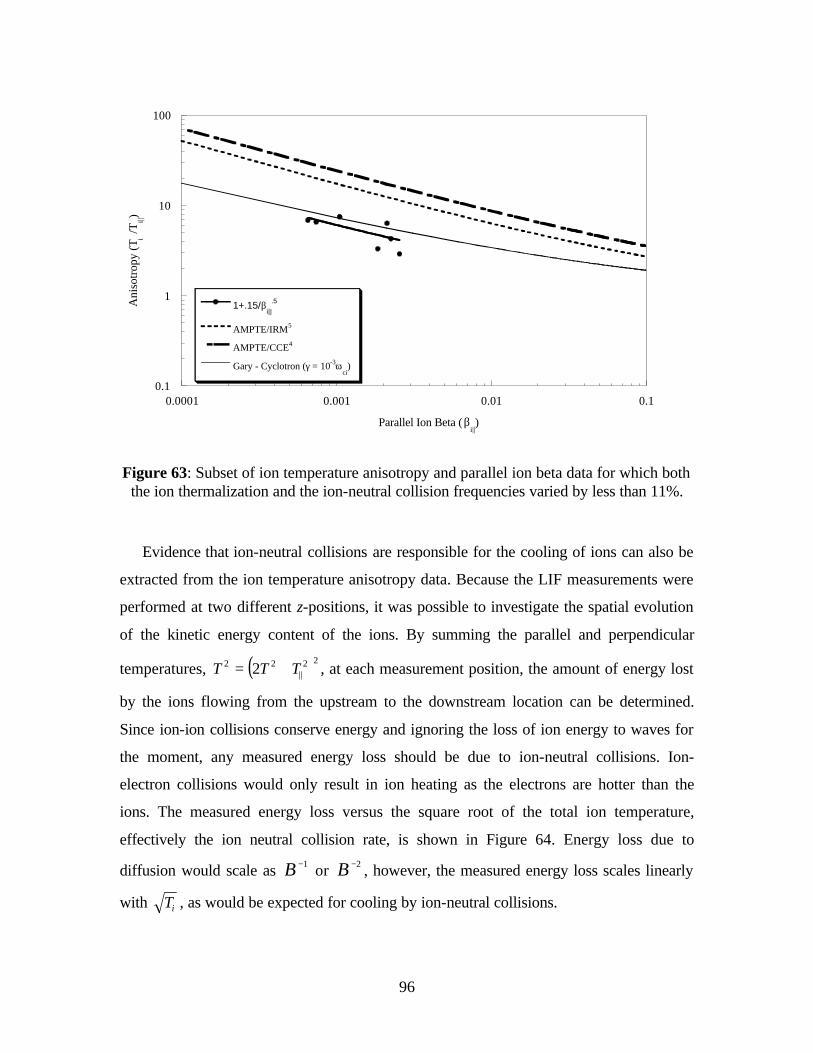
96
0.1
1
10
100
0.0001 0.001 0.01 0.1
1+.15/βi||
.5
AMPTE/IRM5
AMPTE/CCE4
Gary - Cyclotron (γ = 10-3ωci)
Ani
sotr
opy
(Ti ⊥
/Ti||)
Parallel Ion Beta (βi||)
Figure 63: Subset of ion temperature anisotropy and parallel ion beta data for which both the ion thermalization and the ion-neutral collision frequencies varied by less than 11%.
Evidence that ion-neutral collisions are responsible for the cooling of ions can also be
extracted from the ion temperature anisotropy data. Because the LIF measurements were
performed at two different z-positions, it was possible to investigate the spatial evolution
of the kinetic energy content of the ions. By summing the parallel and perpendicular
temperatures, ( )22||
22 2 TTT += ⊥ , at each measurement position, the amount of energy lost
by the ions flowing from the upstream to the downstream location can be determined.
Since ion-ion collisions conserve energy and ignoring the loss of ion energy to waves for
the moment, any measured energy loss should be due to ion-neutral collisions. Ion-
electron collisions would only result in ion heating as the electrons are hotter than the
ions. The measured energy loss versus the square root of the total ion temperature,
effectively the ion neutral collision rate, is shown in Figure 64. Energy loss due to
diffusion would scale as 1−B or 2−B , however, the measured energy loss scales linearly
with iT , as would be expected for cooling by ion-neutral collisions.
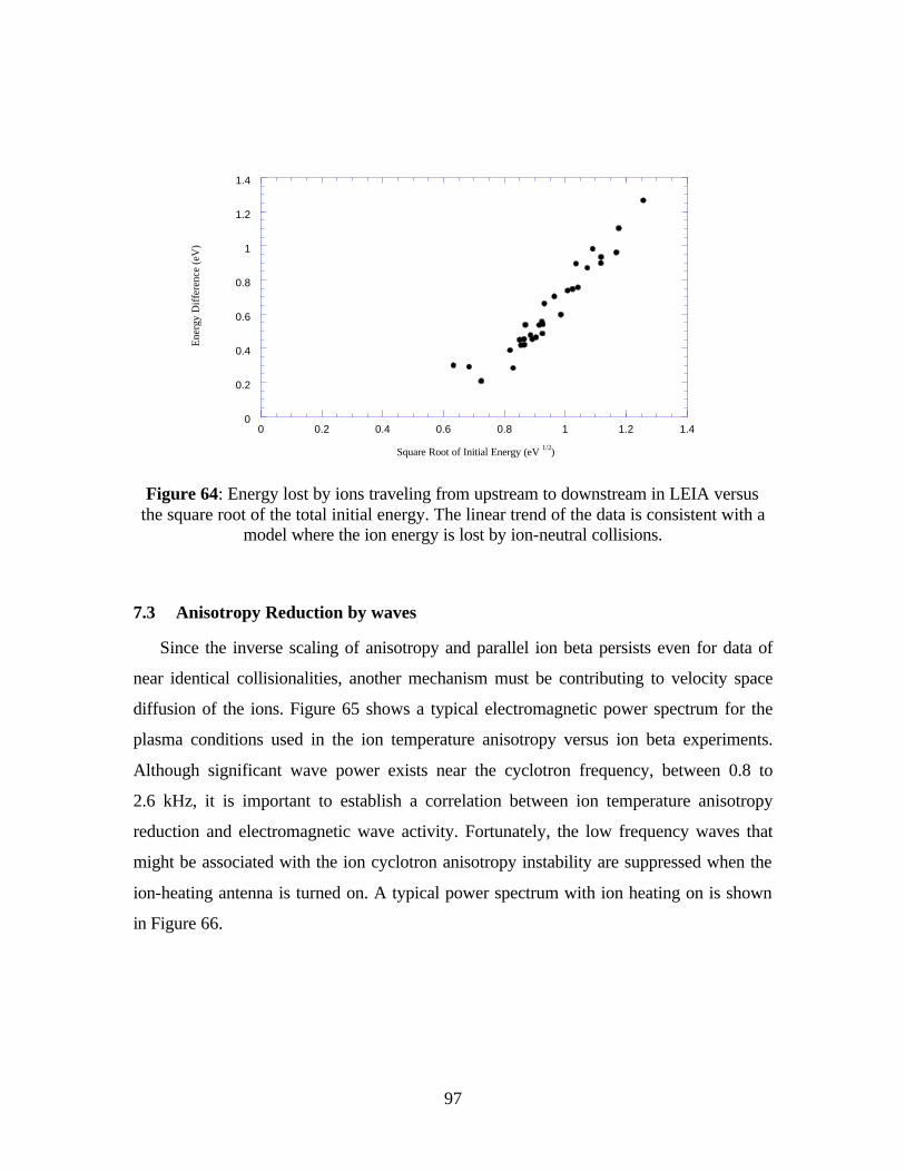
97
0
0.2
0.4
0.6
0.8
1
1.2
1.4
0 0.2 0.4 0.6 0.8 1 1.2 1.4
Ene
rgy
Dif
fere
nce
(eV
)
Square Root of Initial Energy (eV 1/2)
Figure 64: Energy lost by ions traveling from upstream to downstream in LEIA versus the square root of the total initial energy. The linear trend of the data is consistent with a
model where the ion energy is lost by ion-neutral collisions.
7.3 Anisotropy Reduction by waves
Since the inverse scaling of anisotropy and parallel ion beta persists even for data of
near identical collisionalities, another mechanism must be contributing to velocity space
diffusion of the ions. Figure 65 shows a typical electromagnetic power spectrum for the
plasma conditions used in the ion temperature anisotropy versus ion beta experiments.
Although significant wave power exists near the cyclotron frequency, between 0.8 to
2.6 kHz, it is important to establish a correlation between ion temperature anisotropy
reduction and electromagnetic wave activity. Fortunately, the low frequency waves that
might be associated with the ion cyclotron anisotropy instability are suppressed when the
ion-heating antenna is turned on. A typical power spectrum with ion heating on is shown
in Figure 66.

98
10-7
10-5
0.001
0.1
10
1000 104 105
Typical Spectrum
Background
Pow
er (
δB/B
o)2 [H
z-1]
Frequency (Hz)
Figure 65: Typical Br power spectrum of electromagnetic waves during ion temperature anisotropy versus β experiments. The spectrum was obtained without auxiliary ion
heating. The LEIA magnetic field was 66 G.
10-7
10-5
0.001
0.1
10
1000 104 105
Typical Spectrum
Background
Pow
er (
δB/B
o)2 [H
z-2]
Frequency (Hz)
Figure 66: Typical Br power spectrum with ion-heating on. The overall amplitude of low frequency wave activity is much lower than with the heating off. The feature at 33 kHz is
the driving frequency of the ion-heating antenna. The LEIA magnetic field was 66 G.
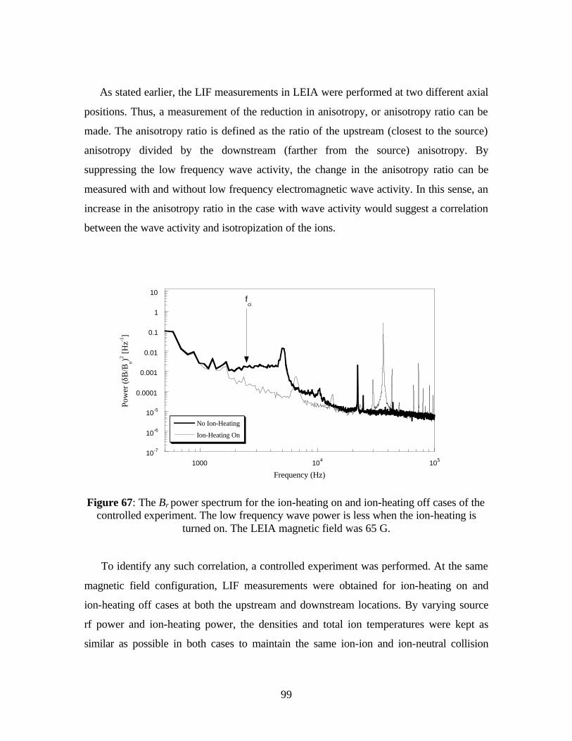
99
As stated earlier, the LIF measurements in LEIA were performed at two different axial
positions. Thus, a measurement of the reduction in anisotropy, or anisotropy ratio can be
made. The anisotropy ratio is defined as the ratio of the upstream (closest to the source)
anisotropy divided by the downstream (farther from the source) anisotropy. By
suppressing the low frequency wave activity, the change in the anisotropy ratio can be
measured with and without low frequency electromagnetic wave activity. In this sense, an
increase in the anisotropy ratio in the case with wave activity would suggest a correlation
between the wave activity and isotropization of the ions.
10-7
10-6
10-5
0.0001
0.001
0.01
0.1
1
10
1000 104 105
No Ion-Heating
Ion-Heating On
Pow
er (δ
B/B
o)2 [H
z-1]
Frequency (Hz)
fci
Figure 67: The Br power spectrum for the ion-heating on and ion-heating off cases of the controlled experiment. The low frequency wave power is less when the ion-heating is
turned on. The LEIA magnetic field was 65 G.
To identify any such correlation, a controlled experiment was performed. At the same
magnetic field configuration, LIF measurements were obtained for ion-heating on and
ion-heating off cases at both the upstream and downstream locations. By varying source
rf power and ion-heating power, the densities and total ion temperatures were kept as
similar as possible in both cases to maintain the same ion-ion and ion-neutral collision

100
frequencies. Figure 67 shows an overlay of the rB power spectra of the heating on and
off cases. When the heating is on, the higher (6 -15 kHz) frequencies are shifted, having a
lower amplitude and the low frequencies ( ciωω ~ ) are suppressed. The only increases in
wave activity are seen at the ion-heating frequency (~ 36 kHz) and its harmonics.
For the heating-on case, 7.53/17 ==downup AA , while for the heating off case,
5.92/19 ==downup AA . Therefore, with the waves present, the anisotropy decreased
more than when the low frequency waves were absent. The heating on case (no waves)
may represent the loss of anisotropy due to collisions. If so, then it appears that when the
waves are present, the amount of isotropization is increased.
10-8
10-6
0.0001
0.01
1
100
1000 104 105
Upstream SignalUpstream BackgroundDownstream SignalDownstream Background
Pow
er (δ
B/B
o)2 [H
z-1]
Frequency (Hz)
fci
Figure 68: Upstream and downstream Br power spectra. Note the higher level of activity for the upstream case. The LEIA magnetic field was 66 G.
Additional evidence in support of the argument that low frequency wave activity
is correlated with ion isotropization can be found in the differences between the
electromagnetic power spectrum measured at the upstream and downstream positions.
Though similar, there are differences between the two power spectra (Figure 68). The

101
upstream measurements show a higher level of wave activity. The fluctuations below ciω
are consistent with the presence of an EMITA instability reducing the ion temperature
anisotropy. It is possible that some of the fluctuations above ciω are also EMITA
instabilities which originate closer to the source where the magnetic field strength is
higher (Figure 22). The anisotropy is lower downstream than it is upstream, thus, the
amplitude of the fluctuations decreases.

102
8 IDENTIFICATION OF THE WAVES
Having established that LEIA plasmas exhibit an inverse correlation between the ion
temperature anisotropy and the parallel ion beta, and that anisotropy reduction is
associated with low frequency wave activity, it is important to determine if the measured
characteristics, frequencies and wavenumbers of the waves are consistent with
predictions for the ion cyclotron anisotropy or mirror instability. Of particular interest are
the waves occurring slightly below the argon cyclotron frequency. For ion cyclotron
anisotropy driven instabilities, the wave frequencies should lie below the ion cyclotron
frequency. The waves should be transverse with wavenumbers of approximately
ck piω~ (see Figure 41).91 For mirror modes, the waves should be extremely low
frequency with wavenumbers of approximately ck pi 2~ ω (see Figure 44).91
8.1 Wave Power Spectra and Amplitude Measurements
Typical spectra of the radial magnetic fluctuations for different HELIX magnetic field
strengths are shown in Figure 70 to Figure 73. At a particular HELIX value of magnetic
field, the spectrum changed from peaked to broadband around 6.5 kHz. However, the
frequency of this main peak is greater than the highest ion gyrofrequency (~2.7 kHz) in
LEIA. Though the higher frequency peaks may be related to the high intrinsic ion
temperatures in LEIA, the primary focus is on electromagnetic waves around or slightly
below the LEIA ion gyrofrequency.

103
10-7
10-6
10-5
0.0001
0.001
0.01
0.1
1
10
102 103 104 105
Pow
er (
δB/B
o)2 [H
z-1]
Frequency (Hz)
Figure 69: Power spectrum of transverse (Br) fluctuations for a HELIX magnetic field of 399 G and a LEIA magnetic field of 65 G. There is a peak near 6.5 kHz and a smaller
peak at roughly 2.5 kHz. The peak at 20 kHz is caused by the pick up of an environmental signal.
10-7
10-6
10-5
0.0001
0.001
0.01
0.1
1
102 103 104 105
Pow
er (
δB/B
o)2 [H
z-1]
Frequency (Hz)
Figure 70: Power spectrum of transverse (Br) fluctuations for a HELIX magnetic field of 556 G and a LEIA magnetic field of 66 G. Note the appearance of the 2nd and 3rd
harmonic of the 6.5 kHz wave.
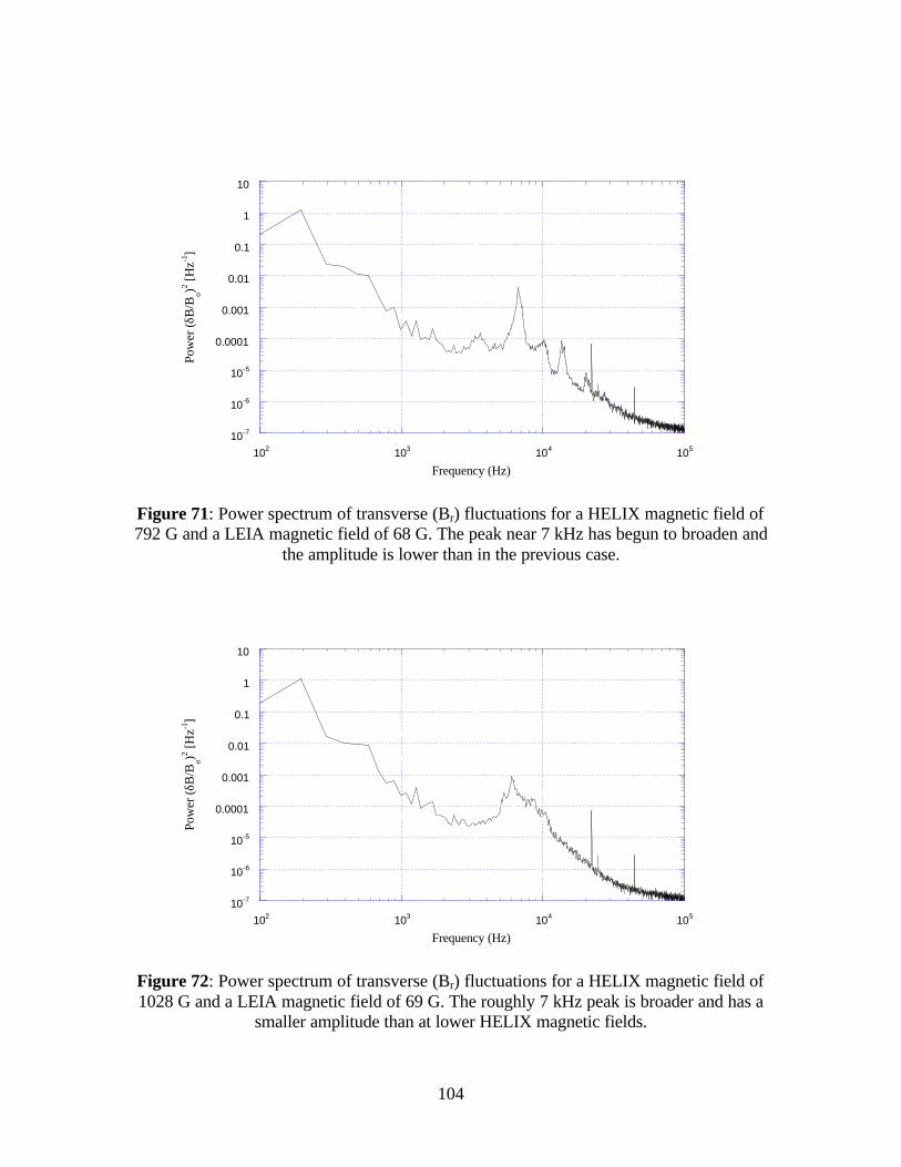
104
10-7
10-6
10-5
0.0001
0.001
0.01
0.1
1
10
102 103 104 105
Pow
er (δ
B/B
o)2 [H
z-1]
Frequency (Hz)
Figure 71: Power spectrum of transverse (Br) fluctuations for a HELIX magnetic field of 792 G and a LEIA magnetic field of 68 G. The peak near 7 kHz has begun to broaden and
the amplitude is lower than in the previous case.
10-7
10-6
10-5
0.0001
0.001
0.01
0.1
1
10
102 103 104 105
Pow
er (δ
B/B
o)2 [H
z-1]
Frequency (Hz)
Figure 72: Power spectrum of transverse (Br) fluctuations for a HELIX magnetic field of 1028 G and a LEIA magnetic field of 69 G. The roughly 7 kHz peak is broader and has a
smaller amplitude than at lower HELIX magnetic fields.

105
10-7
10-6
10-5
0.0001
0.001
0.01
0.1
1
102 103 104 105
Pow
er (δ
B/B
o)2 [H
z-1]
Frequency (Hz)
Figure 73: Power spectrum of transverse (Br) fluctuations for a HELIX magnetic field of 1264 G and a LEIA magnetic field of 70 G. The roughly 7 kHz peak has a smaller
amplitude than previous cases.
Note that the spectral feature at roughly 6.5 kHz changes amplitude and width as the
HELIX magnetic field is changed. This suggests that these waves are a HELIX
phenomenon and not due to LEIA physics. The magnetic field in LEIA was also varied
for each HELIX magnetic field value to identify possible cyclotron features in the
electromagnetic power spectrum. Typical results are shown in Figure 70 and Figure 74
through Figure 76.

106
10-7
10-6
10-5
0.0001
0.001
0.01
0.1
1
10
102 103 104 105
Pow
er (
δB/B
o)2 [H
z-1]
Frequency (Hz)
Figure 74: Transverse (Br) spectrum for a HELIX magnetic field of 556 G and a LEIA magnetic field of 18 G. βi|| ~ .019.
10-7
10-6
10-5
0.0001
0.001
0.01
0.1
1
10
102 103 104 105
Pow
er (δ
B/B
o)2 [H
z-1]
Frequency (Hz)
Figure 75: Transverse (Br) spectrum for a HELIX magnetic field of 556 G and a LEIA magnetic field of 35 G. βi|| ~ .014.
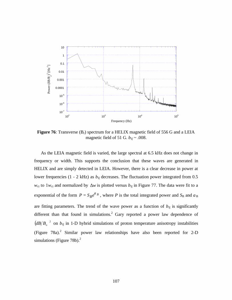
107
10-7
10-6
10-5
0.0001
0.001
0.01
0.1
1
10
102 103 104 105
Pow
er (
δB/B
o)2 [H
z-1]
Frequency (Hz)
Figure 76: Transverse (Br) spectrum for a HELIX magnetic field of 556 G and a LEIA magnetic field of 51 G. βi|| ~ .008.
As the LEIA magnetic field is varied, the large spectral at 6.5 kHz does not change in
frequency or width. This supports the conclusion that these waves are generated in
HELIX and are simply detected in LEIA. However, there is a clear decrease in power at
lower frequencies (1 - 2 kHz) as βi|| decreases. The fluctuation power integrated from 0.5
ωci to 1ωci and normalized by ω∆ is plotted versus βi|| in Figure 77. The data were fit to a
exponential of the form BeSP Bα= , where P is the total integrated power and SB and αB
are fitting parameters. The trend of the wave power as a function of βi|| is significantly
different than that found in simulations.2 Gary reported a power law dependence of
( )2oBBδ on βi|| in 1-D hybrid simulations of proton temperature anisotropy instabilities
(Figure 78a).2 Similar power law relationships have also been reported for 2-D
simulations (Figure 78b).2

108
10-7
10-6
10-5
10-4
10-3
0.0050 0.010 0.015 0.020
y = 6.9229e-08 * e^(398.27x) R= 0.99847
Nor
mal
ized
Int
egra
ted
Wav
e Po
wer
Parallel Ion Beta (βi||)
Figure 77: Integrated wave power for 0.5 to 1.0 ciω normalized by ω∆ and normalized
by the total power in the entire power spectrum for the LEIA magnetic field scan cases. Note, at low values of beta, the data levels off to the noise level, where the low frequency fluctuations are difficult to resolve from the background level. The fit indicates a scaling
of wave power with βi|| that goes roughly as β398e , much stronger than the power law scalings seen in 1-D and 2-D simulations.2
Although there is a clear increase in the low frequency wave power with βi||. At
low values of beta, the normalized integrated wave power levels out. This represents the
noise level, where the low frequency fluctuations are difficult to detect from the
background fluctuation levels. There are some key differences between the simulations
and these experiments. In the simulations, the initial ion temperature anisotropy is held
constant for all values of beta. In the experiment, the ion temperature anisotropy changes
by a factor of four. Integrated broadband wave activity was considered in the
experimental cases, while the simulation results are based on the amplitude scale of a
single spectral feature. It is clear from the experimental data that the low frequency wave
activity increases in amplitude with increasing beta and that the dependence on beta is
much stronger than predicted by the simulation. More realistic simulations are needed
before the wavenumber measurements can be quantitatively compared to the models.
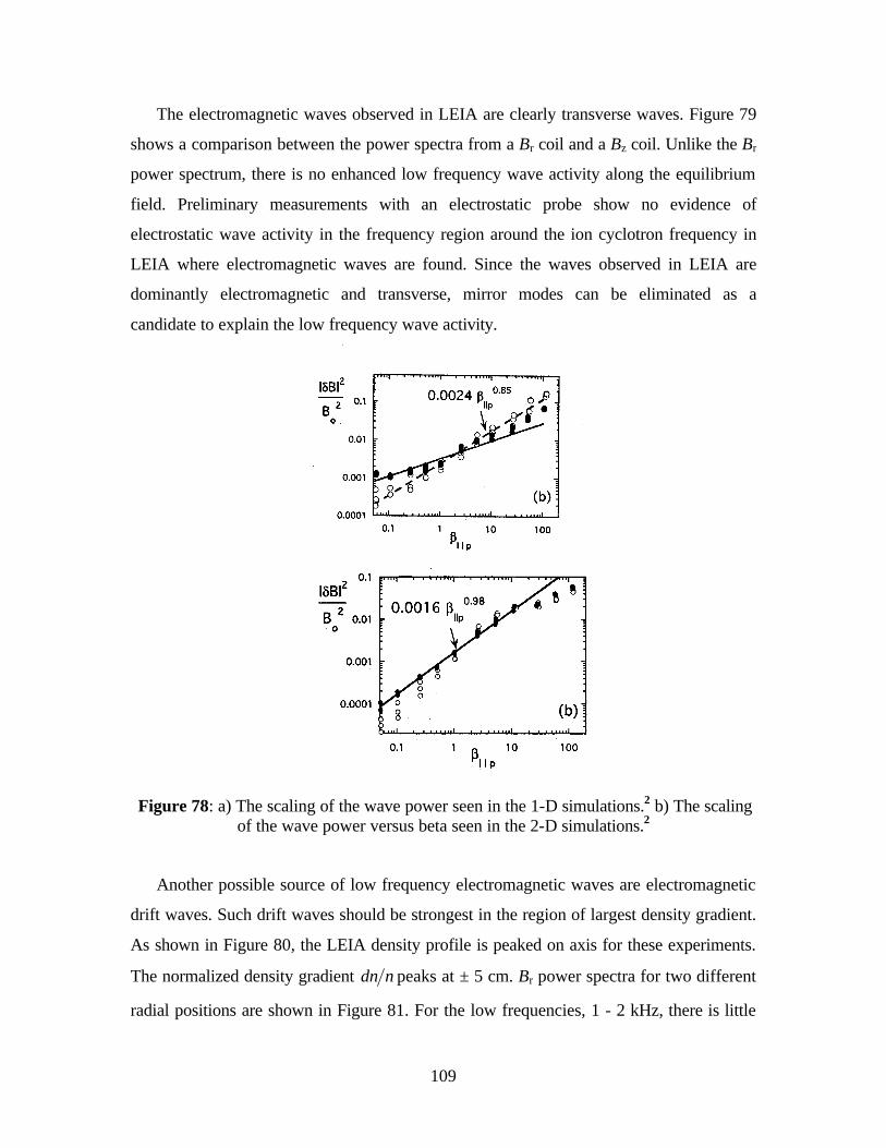
109
The electromagnetic waves observed in LEIA are clearly transverse waves. Figure 79
shows a comparison between the power spectra from a Br coil and a Bz coil. Unlike the Br
power spectrum, there is no enhanced low frequency wave activity along the equilibrium
field. Preliminary measurements with an electrostatic probe show no evidence of
electrostatic wave activity in the frequency region around the ion cyclotron frequency in
LEIA where electromagnetic waves are found. Since the waves observed in LEIA are
dominantly electromagnetic and transverse, mirror modes can be eliminated as a
candidate to explain the low frequency wave activity.
Figure 78: a) The scaling of the wave power seen in the 1-D simulations.2 b) The scaling of the wave power versus beta seen in the 2-D simulations.2
Another possible source of low frequency electromagnetic waves are electromagnetic
drift waves. Such drift waves should be strongest in the region of largest density gradient.
As shown in Figure 80, the LEIA density profile is peaked on axis for these experiments.
The normalized density gradient nnδ peaks at ± 5 cm. Br power spectra for two different
radial positions are shown in Figure 81. For the low frequencies, 1 - 2 kHz, there is little

110
change in the wave power over a change in radius of 24 cm. In addition, even
electromagnetic drift waves should have a significant electrostatic component. The
absence of significant electrostatic wave activity in the ion cyclotron frequency range
further supports the conclusion that the observed waves are not drift waves.
10-7
10-5
0.001
0.1
10
100 1000 104 105
Br Spectrum
Bz Spectrum
Pow
er (
δ B/B
o)2 [H
z-1]
Frequency (Hz)
fci
Figure 79: A Bz power spectrum from the controlled experiment. There are no prominent features visible, unlike a Br spectrum (Figure 65). The feature around 20 kHz is an
artifact that is present when there is no plasma.

111
0
0.2
0.4
0.6
0.8
1
1.2
1.4
-0.1
-0.05
0
0.05
0.1
0.15
-20 -15 -10 -5 0 5 10 15 20
Density
Normalized Density Gradient
Den
sity
(10
12 c
m-3
)
∆
Radius (cm)
n/n
Figure 80: The density profile and normalized density gradient profile for LEIA for a magnetic field of 35 G. The normalized gradient peaks at ± 5 cm.
0.0001
0.001
0.01
0.1
1
10
100
1000 104 105
r = 24 cm
r = 0 cm
Am
plitu
de (
arb
units
)
Frequency (Hz)
fci
Figure 81: Comparison of the Br fluctuation spectra at two different radial positions.
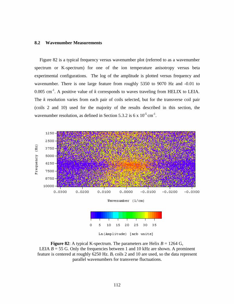
112
8.2 Wavenumber Measurements
Figure 82 is a typical frequency versus wavenumber plot (referred to as a wavenumber
spectrum or K-spectrum) for one of the ion temperature anisotropy versus beta
experimental configurations. The log of the amplitude is plotted versus frequency and
wavenumber. There is one large feature from roughly 5350 to 9070 Hz and -0.01 to
0.005 cm-1. A positive value of k corresponds to waves traveling from HELIX to LEIA.
The k resolution varies from each pair of coils selected, but for the transverse coil pair
(coils 2 and 10) used for the majority of the results described in this section, the
wavenumber resolution, as defined in Section 5.3.2 is 6 x 10⁻⁵ cm-1.
Figure 82: A typical K-spectrum. The parameters are Helix B = 1264 G, LEIA B = 55 G. Only the frequencies between 1 and 10 kHz are shown. A prominent
feature is centered at roughly 6250 Hz. Br coils 2 and 10 are used, so the data represent parallel wavenumbers for transverse fluctuations.

113
To reduce the statistical noise in the wavenumber plot, the data are smoothed with a
running 2-D boxcar average three pixels wide and three pixels long. Figure 83 shows the
results of the smoothing routine applied to the data of Figure 82. To obtain Figure 83,
five smoothing passes were performed. The smoothing accentuates the coherent features
in the data and smoothed plots were used to identify interesting cases for further study.
To determine the wavenumbers associated with a specific frequency or frequency range,
the amplitudes are summed over the frequency range for each wavenumber. To ensure
that peaks appearing in the smoothed data are not artificially created, the wavenumber
spectra for different frequency bands are generated using both the smoothed and
unsmoothed data.
Figure 83: The same data as Figure 82, but smoothed to reduce the background level. There is one very prominent feature on this graph.
The summed amplitude versus wavenumber for frequencies 1 kHz to 10 kHz of the
data shown in Figure 83 is shown in Figure 84 for unsmoothed data and in Figure 85 for
smoothed data. Although for a slightly lower magnetic field, the frequency spectrum for
this case is similar to that shown in Figure 73 - a broad, turbulent regime centered
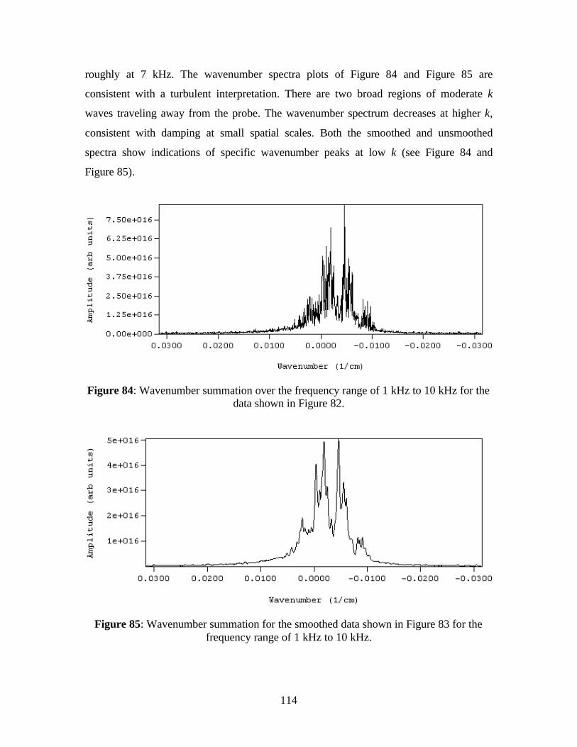
114
roughly at 7 kHz. The wavenumber spectra plots of Figure 84 and Figure 85 are
consistent with a turbulent interpretation. There are two broad regions of moderate k
waves traveling away from the probe. The wavenumber spectrum decreases at higher k,
consistent with damping at small spatial scales. Both the smoothed and unsmoothed
spectra show indications of specific wavenumber peaks at low k (see Figure 84 and
Figure 85).
Figure 84: Wavenumber summation over the frequency range of 1 kHz to 10 kHz for the data shown in Figure 82.
Figure 85: Wavenumber summation for the smoothed data shown in Figure 83 for the frequency range of 1 kHz to 10 kHz.
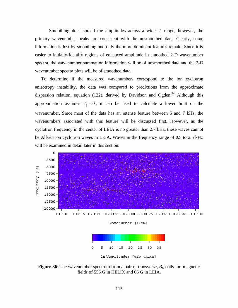
115
Smoothing does spread the amplitudes across a wider k range, however, the
primary wavenumber peaks are consistent with the unsmoothed data. Clearly, some
information is lost by smoothing and only the more dominant features remain. Since it is
easier to initially identify regions of enhanced amplitude in smoothed 2-D wavenumber
spectra, the wavenumber summation information will be of unsmoothed data and the 2-D
wavenumber spectra plots will be of smoothed data.
To determine if the measured wavenumbers correspond to the ion cyclotron
anisotropy instability, the data was compared to predictions from the approximate
dispersion relation, equation (122), derived by Davidson and Ogden.94 Although this
approximation assumes 0|| =T , it can be used to calculate a lower limit on the
wavenumber. Since most of the data has an intense feature between 5 and 7 kHz, the
wavenumbers associated with this feature will be discussed first. However, as the
cyclotron frequency in the center of LEIA is no greater than 2.7 kHz, these waves cannot
be Alfvén ion cyclotron waves in LEIA. Waves in the frequency range of 0.5 to 2.5 kHz
will be examined in detail later in this section.
Figure 86: The wavenumber spectrum from a pair of transverse, Br, coils for magnetic fields of 556 G in HELIX and 66 G in LEIA.
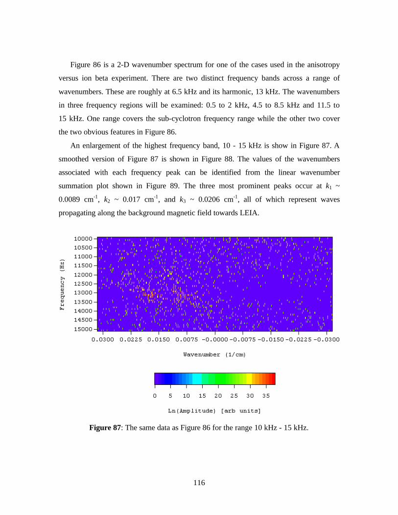
116
Figure 86 is a 2-D wavenumber spectrum for one of the cases used in the anisotropy
versus ion beta experiment. There are two distinct frequency bands across a range of
wavenumbers. These are roughly at 6.5 kHz and its harmonic, 13 kHz. The wavenumbers
in three frequency regions will be examined: 0.5 to 2 kHz, 4.5 to 8.5 kHz and 11.5 to
15 kHz. One range covers the sub-cyclotron frequency range while the other two cover
the two obvious features in Figure 86.
An enlargement of the highest frequency band, 10 - 15 kHz is show in Figure 87. A
smoothed version of Figure 87 is shown in Figure 88. The values of the wavenumbers
associated with each frequency peak can be identified from the linear wavenumber
summation plot shown in Figure 89. The three most prominent peaks occur at k1 ~
0.0089 cm-1, k2 ~ 0.017 cm-1, and k3 ~ 0.0206 cm-1, all of which represent waves
propagating along the background magnetic field towards LEIA.
Figure 87: The same data as Figure 86 for the range 10 kHz - 15 kHz.

117
Figure 88: Smoothed version of the data shown in Figure 87. After smoothing, two distinct peaks area clearly visible.
Figure 89: Wavenumber summation of Figure 88 on a linear scale. Three large peaks occur at higher wavenumbers. These are waves propagating towards LEIA.

118
Figure 90 is an enlargement of the data in Figure 86 between frequencies of 5 kHz
and 8 kHz. In the smoothed plot of
Figure 91, two clusters of peaks centered about 6.5 kHz are clearly visible. Unlike
the 13 kHz feature, the 6.5 kHz features lie in the negative k region. Figure 92 shows the
wavenumber summation for the 5 - 8 kHz band on a linear scale. Like the 13 kHz feature,
this frequency band contains two broad wavenumber peaks and a smaller amplitude,
narrow wavenumber peak. However, the 5 - 8 kHz waves are all propagating upstream
towards LEIA. Note the improvement in signal to noise ratio for the 5 - 8 kHz waves
compared to the 10 - 15 kHz waves.
Figure 90: The same data as in Figure 86, but for the frequency range of 5 kHz to 8 kHz.

119
Figure 91: Smoothed version of the data shown in Figure 90. After smoothing, two
distinct peaks are clearly visible.
Figure 92: The wavenumber summation over 5 - 8 kHz for the data of Figure 90.
To determine if ion cyclotron anisotropy instabilities could be identified, the
experimental cases for a fixed HELIX magnetic field and different LEIA magnetic fields
were examined. Figure 93 shows the low frequency region of the 2D wavenumber

120
spectrum for the case of a LEIA magnetic field of 66 G, a HELIX field of 556 G, and an
ion temperature anisotropy of 6.9. Even in the smoothed data shown in Figure 94, it is not
possible to visually identify any enhancements at a specific frequency or wavenumber.
The wavenumber summation shown in Figure 95 highlights the poor signal to noise ratio
at these low frequencies. Fundamentally, the difficulty in measuring wavenumbers at low
frequencies is sensitivity. The signal generated by a magnetic sense coil varies linearly
with both amplitude and the frequency of the fluctuating wave. The lower the frequency
of the wave, the smaller the sense coil signal. Therefore, the best chance of obtaining
wavenumber measurements of ion cyclotron anisotropy instabilities should occur at the
highest LEIA fields possible (to raise the gyrofrequency to a region of better sensitivity)
and the highest ion temperature anisotropy possible (to increase the wave amplitude).
Figure 93: Enlargement of the frequency range of 0.6 to 2.6 kHz for the same data shown in Figure 86.

121
Figure 94: Same data as Figure 93 after smoothing. There are no distinct spectral features.
Figure 95: The wavenumber summation over .6 to 2.6 kHz for the data of Figure 93.
Figure 96 shows the normalized wavenumber summation from 1 - 2.7 kHz for a
HELIX field of 1264 G, a LEIA field of 70 G, and an ion temperature anisotropy of 8.3.
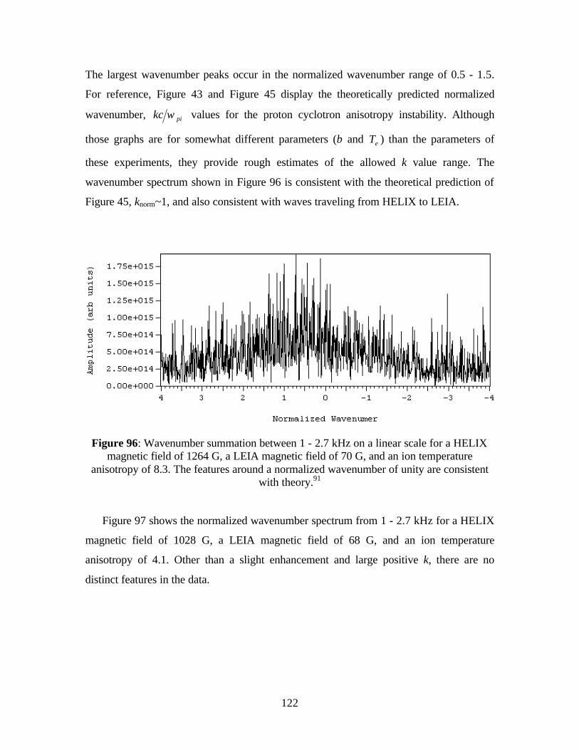
122
The largest wavenumber peaks occur in the normalized wavenumber range of 0.5 - 1.5.
For reference, Figure 43 and Figure 45 display the theoretically predicted normalized
wavenumber, pikc ω values for the proton cyclotron anisotropy instability. Although
those graphs are for somewhat different parameters (β and eT ) than the parameters of
these experiments, they provide rough estimates of the allowed k value range. The
wavenumber spectrum shown in Figure 96 is consistent with the theoretical prediction of
Figure 45, knorm~1, and also consistent with waves traveling from HELIX to LEIA.
Figure 96: Wavenumber summation between 1 - 2.7 kHz on a linear scale for a HELIX magnetic field of 1264 G, a LEIA magnetic field of 70 G, and an ion temperature
anisotropy of 8.3. The features around a normalized wavenumber of unity are consistent with theory.91
Figure 97 shows the normalized wavenumber spectrum from 1 - 2.7 kHz for a HELIX
magnetic field of 1028 G, a LEIA magnetic field of 68 G, and an ion temperature
anisotropy of 4.1. Other than a slight enhancement and large positive k, there are no
distinct features in the data.

123
Figure 97: Wavenumber summation between 1 - 2.7 kHz on a linear scale for a HELIX magnetic field of 1028 G, a LEIA magnetic field of 38 G, and an ion temperature
anisotropy of 4.1.
Figure 98 shows the wavenumber summation from 1 - 2.7 kHz for a HELIX magnetic
field of 792 G, a LEIA magnetic field of 68 G, and an ion temperature anisotropy of 7.3.
This case does not have as broad of a range of wavenumbers as Figure 96, but the
positive k portion of the spectrum is clearly enhanced. The three largest peaks occur at
normalized wavenumbers of roughly 0.6, 1.4, and 2.5. The 0.6 - 1.4 peaks are consistent
with the theory predictions of Figure 45.
Figure 98: Wavenumber summation between 1 - 2.7 kHz on a linear scale for a HELIX magnetic field of 792, a LEIA magnetic field of 68 G and an anisotropy of 7.3.
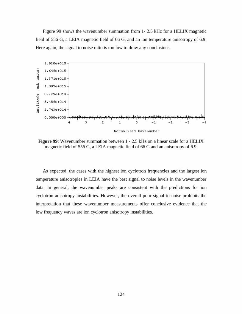
124
Figure 99 shows the wavenumber summation from 1- 2.5 kHz for a HELIX magnetic
field of 556 G, a LEIA magnetic field of 66 G, and an ion temperature anisotropy of 6.9.
Here again, the signal to noise ratio is too low to draw any conclusions.
Figure 99: Wavenumber summation between 1 - 2.5 kHz on a linear scale for a HELIX magnetic field of 556 G, a LEIA magnetic field of 66 G and an anisotropy of 6.9.
As expected, the cases with the highest ion cyclotron frequencies and the largest ion
temperature anisotropies in LEIA have the best signal to noise levels in the wavenumber
data. In general, the wavenumber peaks are consistent with the predictions for ion
cyclotron anisotropy instabilities. However, the overall poor signal-to-noise prohibits the
interpretation that these wavenumber measurements offer conclusive evidence that the
low frequency waves are ion cyclotron anisotropy instabilities.

125
9 DISCUSSION
These experiments demonstrate the existence of an inverse correlation between the
ion temperature anisotropy and the parallel ion beta in a high beta laboratory plasma. The
scaling of the correlation is in good agreement with both theoretical models and
spacecraft observations for ion temperature anisotropies limited by the action of
electromagnetic ion temperature anisotropy instabilities. The apparent universality of the
inverse correlation between ion temperature anisotropy and parallel ion beta supports
Manheimer and Boris' claim that a plasma instability threshold derived from linear theory
should correspond to an observable bound on the ion temperature anisotropy.
To reduce the possible effect of varying the collisionality in interpreting this
marginally collisional laboratory experiment, a subset of data with roughly the same ion-
neutral collision and ion-ion thermalization rates was identified. Within that data subset,
the inverse correlation was still observed. The effect of low frequency waves on the
reduction of anisotropy between upstream and downstream positions was studied in a
controlled experiment. The amount of anisotropy reduction decreased when the
amplitudes of low frequency electromagnetic waves decreased. This suggests that the low
frequency waves are related to the anisotropy reduction observed in LEIA. Magnetic
fluctuation spectra of the low frequency waves demonstrated an exponential scaling of
the low frequency electromagnetic wave power with ion beta. The exponential nature of
the wave power scaling is in contrast to the power law scaling predicted by theory. The
electromagnetic wave measurements clearly indicate that the low frequency waves are
transverse, not compressional. In the experimental cases with the highest cyclotron
frequencies and the highest ion temperature anisotropies, the observed wavenumbers are
consistent with the wavenumber values predicted for ion cyclotron anisotropy
instabilities. Although these low frequency fluctuations can not be conclusively identified
as ion cyclotron anisotropy waves because of poor signal to noise ratio in the
wavenumber measurements, the observed characteristics of these waves suggest the
waves are most consistent with ion cyclotron anisotropy instabilities.
126
To enable better identification of low frequency waves in LEIA, there are a number of
experimental modifications that could be implemented. Fundamentally, the signal-to-
noise ratio below 3 kHz can be improved. One way of accomplishing this is by increasing
the number of turns on the magnetic sense coils, which will increase the sensitivity at
lower frequencies. Taking more realizations than the fifty used in these studies will also
improve the signal-to-noise ratio in the wavenumber analysis. Reducing the sampling
rate, would improve frequency space resolution and accentuate features in the power
spectra of the low frequency waves. With better signal-to-noise, the polarization of the
low frequency waves could be determined with hodograms constructed from Br and Bθ
data. As the wavenumber measurements presented here indicate the wavelengths in LEIA
are on the order of a few meters, wavenumber measurements with larger probe
separations would provide improved phase difference sensitivity.
Detailed electrostatic probe measurements over the parameter range used in these
experiments will play a key role in verifying that the low frequency waves are indeed
primarily electromagnetic. Development of LIF techniques to identify electromagnetic
waves through perturbations of the ion distribution function could also be used in
conjunction with magnetic sense coils observations to better identify low frequency
waves.

127
10 REFERENCES
1 Manheimer, W. and J. P. Boris, "Marginal stability analysis – A simpler approach to anomalous transport
in plasmas," Comments Plasma Phys. Controlled Fusion, 3, 15 (1977). 2 Gary, S. P., J. Wang, D. Winske, and S. A. Fuselier, "Proton temperature anisotropy upper bound," J.
Geophys. Res., 102, 27159 (1997). 3 Gary, S. Peter, Michael E. McKean, Dan Winske, Brian J. Anderson, Richard E. Denton and Stephen A.
Fusilier, "The proton cyclotron instability and the anisotropy/β inverse correlation," J. Geophys. Res., 99, 5903 (1994).
4 Anderson, Brian J., Stephan A. Fuselier, S. Peter Gary, and Richard E. Denton, "Magnetic spectral signatures in the Earth’s magnetosheath and plasma depletion layer," 99, J. Geophys. Res. 5877 (1994).
5 Phan, T.-D., G. Paschmann, W. Baumjohann, N. Sckopke, and H. Luhr, "The magnetosheath region adjacent to the dayside magnetopause: AMPTE/IRM observations," J. Geophys. Res., 99, 121 (1994).
6 Fuselier, Stephan A., Brian J. Anderson, S. Peter Gary, and Richard E. Denton, "Inverse correlations between the ion temperature anisotropy and plasma beta in the Earth’s quasi-parallel magnetosheath," J. Geophys. Res., 99, 14,931 (1994).
7 Scharer, J. E., and A. W. Trivelpiece, "Cyclotron wave instabilities in a plasma," Phys. Fluids, 10, 591 (1967).
8 Nakamura, Motoyuki et al., "Excitation of the Alfvén ion cyclotron mode soley by the ion pressure distribution," Jpn. J. Appl. Phys., 37, 342 (1998).
9 Casper, T. A., and Gary R. Smith, "Observation of Alfvén Ion-CyclotronFluctuations in the End-Cell Plasma in the Tandem Mirror Experiment," 48, 1015 (1982).
10 Kivelson, Margaret G., and Christopher T. Russell, "Introduction to Space Physics," Cambridge University Press (1995).
11 Hill, K. W, et al., "Tests of local transport theory and reduced wall impurity influx with highly radiative plasmas in the Tokamak Fusion Test Reactor," Phys. Plasmas, 6, 877 (1999).
12 Greenwald, et al., "Characterization of enhanced Dα high-confinement modes in Alcator C-Mod", Phys. Plasmas, 6, 1943 (1999).
13 Chen, Francis F., "Introduction to plasma physics and controlled fusion," Plenum Press (1984). 14 Chevalier, G, and F. F. Chen, "Experimental modeling of inductive discharges", J. Vac. Sci. Technol. A.,
11, 1165 (1993). 15 Chen, Francis F., "Capacitor tuning circuits for inductive loads", UCLA Internal Report PPG-1401, 1992. 16 Balkey, M, " Investigation of different antenna designs on HELIX," WVU Internal Report (1999). 17 Kline, John, E. E. Scime, P. A. Keiter, M. M. Balkey, R. F. Boivin, "Ion heating in the HELIX helicon
plasma source," submitted to Phys. Plasmas, (1999). 18 Light, Max, Isaac D. Sudit, Francis F. Chen, and Donald Arnush, "Axial propagation of helicon waves,"
Phys. Plasmas, 2, 4094 (1995). 19 Guo, X. M., J. Scharer, Y. Mouzouris, and L. Louis, "Helicon experiments and simulations in
nonuniform magnetic field configurations," University of Wisconsin Internal Report, UW-CPTC 98-14, (1998).
20 Shoji, T, Y. Sakawa, S. Nakazawa, K. Kadota, and T. Sato, "Plasma production by helicon waves," Plasma Sources Sci. Technol., 2, 5 (1993).
21 Boswell, R.W., "Plasma Production using a standing helicon wave," Physics Letters, 33A, 457 (1970). 22 Perry, A.J., D. Vender, and R. W. Boswell, "The application of the helicon source to plasma processing,"
J. Vac. Sci. Technol. B, 9, 310 (1991). 23 Jiwari, Nobuhiro, Hiroaki Isasawa, Akira Narai, Hiroyuki Sakaue, Haruo Shindo, Tatsuo Shoji and
Yasuhiro Horiike, "Al etching characteristics employing helicon wave plasma," Jpn. J. Appl. Phys., 32, 3019 (1993).

128
24 Katyukha, V. P., G. S. Kirichenko, A. V. Rusavskii, V. B. Taranov and K. P. Shamrai, "Helicon ion
source for plasma processing," Rev. Sci. Instrum., 65, 1368 (1994). 25 Mieno, T., T. Kamo, D. Hayashi, T. Shoji and K. Kadota, "Efficient production of O+ and O- in a helicon
wave oxygen discharge," Appl. Phys. Lett., 69, 617 (1996). 26 Tsukada, Tsutomu, Hiroshi Nogami, Jun Hayashi, Kazu Kawaguchi and Toru Hara, "Physical damage in
silicon formed by helicon wave plasma etching," J. Appl. Phys., 74, 5402 (1993). 27 Shats, M. G., D. L. Rudakov, R. W. Boswell, and G. G. Borg, "Ion temperature and plasma flows in
improved confinement mode in the H-1 heliac," Phys. Plasmas, 4, 3629 (1997). 28 Chang-Diaz, F. R., R. H. Goulding, R. D. Bengtson, F. Wally-Baity, D. Sparks, R. G. Russel Jr., G. C.
Barber, G. McCaskill, V. T. Jacobson, M. D. Carter, A. V. Ilin, T. W. Glover, "Experimental status of the development of a variable specific impulse magnetoplasma rocket," Fusion Technology, 35, 243 (1999).
29 Aigrain, P., "Les 'helicons' dans les semiconducteurs," Proc. Int. Conf. Seniconductor Physics, 224, (1960).
30 Legendy, C. R., "Macroscopic theory of helicons," Phys. Rev., 135, 1713 (1965). 31 Klosenberg, J. P., B. McNamara and P. C. Thoneman, "The dispersion and attenuation of helicon waves
in a uniform cylindrical plasma," J. Fluid Mech., 21, 545 (1965). 32 Boswell, R. W., "Modulated rf produced argon magneto-plasma," The Flinders University of South
Australia Internal Rep., PR 68/8, 1968. 33 Boswell, Rod W., and Francis F. Chen, "Helicons – The early years," IEEE Transactions on Plasma
Science, 25, 1229 (1997). 34 Zhu, Peiyuan and R. W. Boswell, "Observation of nonthermal electron tails in an rf exited argon
magnetoplasma," Phys. Fluids B, 3, 869 (1991). 35 Boswell, R.W., "Very efficient plasma generation by whistler waves near the lower hybrid frequency,"
Plasma Phys. Control. Fusion, 26, 1147 (1984). 36 Ellingboe, A. R., and R. W. Boswell, "Capacitive, inductive and helicon-wave modes of operation of a
helicon plasma source," Phys. Plasmas, 3, 2797 (1996). 37 Keiter, Paul A., Earl E. Scime, and Matthew M. Balkey, "Frequency dependent effects in helicon
plasmas," Phys. Plasmas, 4, 2741 (1997). 38 Shoji, T., IPPJ Annu. Rev., Nagoya Univ., Japan, 67 (1986). 39 Suddit, Isaac D., and Francis F. Chen, "Discharge equilibrium of a helicon discharge," Plasma Sources
Sci. Technol., 5, 43 (1995). 40 Guo, X. M., J. Scharer, Y. Mouzouris and L. Louis, "Helicon experiments and simulations in nonuniform
magnetic field configurations," Phys. Plasmas, 6, 3400 (1999). 41 Klinger, Thomas, "Control of plasma instabilities in laboratory plasmas," IPELS meeting, 1999. 42 Watts, Christopher, "Laboratory Alfvén wave measurements in a steady state, high-density plasma,"
P.3.10, IPELS meeting, 1999. 43 Stix, T. H., "Waves in Plasmas" (American Institute of Physics, New York, 1992). 44 Borg, G. G. and R. W. Boswell, " Power coupling to helicon and Trivelpiece-Gould modes in helicon
sources," Phys. Plasmas, 5, 564 (1998). 45 Chen, Francis F., "Plasma ionization by helicon waves," Plasma Phys. And Contr. Fus., 33, 339 (1991). 46 Yun, Seok-Min, Jung-Hyung Kim and Hong-Young Chang, "Frequency dependence of helicon wave
plasmas near lower hybrid resonance frequency," J. Vac. Sci. Technol. A., 15, 673 (1997). 47 Komori, A., T. Shoji, K. Miyamoto, J. Kawai, Y. Kawai, "Helicon waves and efficient plasma
production," Phys. Fluids B, 3, 893 (1991). 48 Chen, Francis, F., Hsieh, M. Johannes, and Max Light, "Helicon waves in a non-uniform plasma,"
Plasma Sources Sci. Technol., 3, 49 (1994). 49 Chen, Francis F., "Experiments on helicon plasma sources," J. Vac. Sci. Technol. A, 10, 1389 (1992). 50 Jackson, J., "Classical Electrodynamics," John Wiley & Sons Inc., New York, (1975) 51 Chen, Francis F., and Christopher D. Decker, "Electron Acceleration in Helicon Sources," Plasma
Physics and Controlled Fusion, 34, 635 (1992).
129
52 Molvik, A.W., A. R. Ellingboe and T. D. Rognmien, "Hot-Electron Production and Wave Structure in a
Helicon Plasma Source," Physical Review Letters, 79, 233 (1997). 53 Chen, Francis F. and David D. Blackwell, "Upper limit to Landau damping in helicon discharges,"
UCLA Internal Report LTP-809, 1998. 54 Degeling, A. W., C. O. Jung, R. W. Boswell, and A. R. Ellingboe, "Plasma production from helicon
waves," 3, 2788 (1996) 55 Chen, F. F., X. Jiang, J. D. Evans, G. Tynan, and D. Arnush, "Low field helicon discharges," UCLA
Internal Report PPG-1564 (1996). 56 Chen, F. F., and G. Chevalier, "Experiments on helicon plasma sources," J. Vac. Sci. Technol. A, 10,
1389 (1992). 57 Davies, B., "Helicon wave propagation: effect of electron inertia," J. Plasma Physics, 4, 43 (1970). 58 Boswell, R. W., "Dependence of helicon wave radial structure on electron inertia," Aust. J. Phys., 25,
403 (1972). 59 Shamrai, K. P., and V. B. Taranov, "Resonance wave discharge and collisional energy absorption in
helicon plasma source," Plasma Phys. Control. Fusion, 36, 1719 (1994). 60 Chen, Francis F. and Rod W. Boswell, "Helicons – The past decade," IEEE Transactions on Plasma
Science, 25, 1245 (1997). 61 Hutchinson, I. H., "Principles of Plasma Diagnostics," Cambridge University Press, 1987. 62 Krall, Nicholas A., and Alvin W. Trivelpiece, "Principles of plasma physics," San Francisco Press, 1986. 63 Boschi, A. and Magistrelli, F., Nuovo Cimento, 29, 487 (1962). 64 Hershkowitz, N., M. H. Cho, C. H. Nam, and T. Intrator, " Langmuir probe characteristics in RF glow
discharges ," Plasma Chem. And Plasma Proc. 8, 35 (1988). 65 Sudit, Isaac D. and Francis F. Chen, "RF compensated probes for high-density discharges," Plasma
Sources Sci. Techol., 3, 162 (1994). 66 Godyak, V. A., R. B. Piejak, and B. M. Alexandrovich, " Measurement of electron energy distribution in
low-pressure RF discharges" Plasma Sources Sci. Technol., 1, 36 (1992). 67 Measures, R. M., "Selectrive excitation spectroscopy and some possible apllications," J. Appli. Phys., 39,
5232 (1968). 68 Skiff, F., and F. Anderegg, " Direct observation of plasma dielectric motion ," Phys. Rev. Lett. 59, 896
(1987). 69 Sarfaty, M., S. De Souza-Machado, and F. Skiff, " Direct determination of ion wave fields in a hot
magnetized and weakly collisional plasma," Phys. Plasmas 3, 4316 (1996). 70 McChesney, Jon Mearns, "Observation of stochastic ion heating by low frequency drift waves," Ph.D.
Thesis (1989). 71 Moore, C. A., G. P. Davis and R. A. Gottscho, "Sensitive, nonintrusive in-situ measurement of
temporally and spatially resolved plasma electric fields," Phys. Rev. Lett., 52, 538 (1984). 72 West, W. P., D. M. Thomas. E. S. Ensberg, J. S. DeGrassie, and J. F. Baur, "Diagnostic instrument for
the measurement of poloidal magnetic fields in tokamaks," Rev. Sci. Instr., 57, 1552 (1986). 73 Boivin, R. F., "Study of the different line broadening mechanisms for the laser induced fluorescence
diagnositic for the HELIX and LEIA plasmas," WVU Internal Report PL-039, (1998). 74 Wise, W. L., "Line Broadening," Plasma Diagnostic techniques ed. By Richard H. Huddlestone and
Stanley L. Leonard, 269 (1965). 75 Griem, H. R., "Plasma Spectroscopy," McGraw-Hill, New York, (1964). 76 Demtroder, W., "Laser Spectroscopy," Spinger Verlag (1981). 77 Goeckner M. J., and J. Goree, "Laser-induced fluorescence measurement of plasma ion temperatures:
corrections for power saturation," J. Vac. Sci. Technol. A, 7, 977 (1989). 78 J. M. Beall, Y. C. Kim, and E.J. Powers, "Estimation of wavenumber and frequency spectra using fixed
probe pairs," J. Appl. Phys., 53, 3993 (1982). 79 Bendat, Julius S., and Allan G. Piersol, "Engineering applications of correlation and spectral analysis,"
John Wiley & Sons Inc., (1980). 80 Hundhausen, A. J., J. R. Asbridge, S. J. Bame, H. E. Gilbert and I. B. Strong, "Vela 3 satellite
observations of solar wind ions: A priliminary report," J. Geophys. Res., 72, 87 (1967).

130
81 Wolfe, J. H., R. W. Silva, D. D. McKibbin and R. H. Mason, "The compositional, anisotropic and
nonradial-flow characteristics of the solar wind," J. Geophys. Res., 71, 3329 (1966). 82 Scarf, F. L., J. H. Wolfe, and R. W. Silva, "A plasma instability associated with thermal anisotropies in
the solar wind," J. Geophys. Res., 72, 993 (1967). 83 Holzer, R. E., M. G. McLeod and E. J. Smith, "Preliminary results from the OGO 1 search coil
magnetometer; Boundary positions and magnetic noise spectra," J. Geophys. Res., 71, 1481 (1966). 84 Coleman, P. J., Jr. "Variations in the interplanetary magnetic field: Mariner 2, 1, Observed properties," J.
geophys. Res., 71, 5509 (1966). 85 Siscoe, G. L., L. Davies Jr., P. J. Coleman Jr., E. J. Smith and D. E. Jones, "Power Spectra and
discontinuities of the interplanetary magnetic field: Mariner 4,"J. Geophys. Res., 73, 61 (1968). 86 Ness, N. F., G. S. Scearce and S. Cantarano, "Preliminary results from the Pioneer 6 magnetic field
exponent," J. Geophys. Res., 71, 3305 (1966). 87 Kennel, C. F. and H. E. Petschek, "Limit on stabley trapped particle fluxes," J. Geophys. Res., 71, 1
(1966). 88 Chandrasekhar, S., A. N. Kaufman, and K. M. Watson, "The stability of the pinch," Proc. Roy. Soc.
London, Ser. A., 245, 435 (1958). 89 Barnes, A., "Collisionless damping of hydromagnetic waves," Phys. Fluids, 9, 1483 (1966). 90 Fried, B. D., and S. D. Conte, "The Plasma Dispersion Relation," Academic Press, New York (1961). 91 Gary, S. P., "Theory of Space Plasma Microinstabilities," Cambridge University Press, Cambridge
(1993). 92 McKean., M. E., D. Winske, and S. P. Gary, "Mirror and ion cyclotron anisotropy instabilities in the
magnetosheath," J. Geophys. Res., 97, 19421 (1992). 93 Price, C. P., D. W. Swift, and L.-C. Lee, "Numerical simulations of nonoscillatory mirror waves at the
Earth’s magnetosheath," J. Geophys. Res., 91, 101 (1986). 94 Davidson, R. C., and Joan M. Ogden, "Electromagnetic ion cyclotron instability driven by ion energy
anisotropy in high-beta plasmas,",Phys. Fluids, 18, 1045 (1975). 95 Winske, D., and N. Omidi, "Hybrid codes: Methods and applications, in Computer Space Plasma
Physics: Simulation Techniques and Software," edited by H. Matsumoto and Y. Omura, Terra Scientific, Tokyo (1992).
96 McKean, M. E., D. Winske, S. P. Gary, "Two-dimensional simulations of ion anisotropy instabilities in the magnetosheath," J. Geophys. Res., 99, 11,141 (1994).
97 Gary, S. Peter, Michael E. McKean, Dan Winske, Brian J. Anderson, Richard E. Denton and Stephen A. Fusilier, "The proton cyclotron instability and the anisotropy/β inverse correlation," J. Geophys. Res., 99, 5903 (1994).
98 Gary, S. Peter. Private Communication (1999). 99 Gary, S. Peter, Brian J. Anderson, Richard E. Denton, Stephen A. Fuselier and Michael E. McKean, "A
limited closure relation for anisotropic plasmas from the Earth's magnetosheath," Phys. Plasmas, 1, 1676 (1994).
100 Anderson. B. J., and S. A. Fuselier, "Magnetic pulsations from 0.1 to 4.0 Hz and associated plasma properties in the Earth’s subsolar magnetosheath and plasma depletion layer," J. Geophys. Res., 98, 1461 (1993).
101 Song, Paul, Private Communication (1999). 102 Anderson, B. J., T. -D. Phan, and S. A. Fuselier, "Relationships between plasma depletion and subsolar
reconnection," J. Geophys. Res., 102, 9531 (1997). 103 Anderson, Brian J., Stephan A. Fuselier, S. Peter Gary, and Richard E. Denton, "Magnetic spectral
signatures in the Earth’s magnetosheath and plasma depletion layer," 99, J. Geophys. Res. 5877 (1994). 104 Phan, T.-D., G. Paschmann, W. Baumjohann, N. Sckopke, and H. Luhr, "The magnetosheath region
adjacent to the dayside magnetopause: AMPTE/IRM observations," J. Geophys. Res., 99, 121 (1994). 105 Phan, T. D., et al, "The subsolar magnetosheath and magnetopause for high solar wind ram pressure:
WIND observations," Geophys. Res. Lett., 23, 1279 (1996).

131
106 Fuselier, Stephan A., Brian J. Anderson, S. Peter Gary, and Richard E. Denton, "Inverse correlations
between the ion temperature anisotropy and plasma beta in the Earth’s quasi-parallel magnetosheath," J. Geophys. Res., 99, 14,931 (1994).
107 Inutake, M. et al, " Thermal barrier formation and plasma confinement in the axisymmetrized tandem mirror GAMMA 10," Phys. Rev. Lett., 55, 939 (1985).
108 Casper, T. A. and Gary R. Smith, "Observation of Alfvén ion-cyclotron fluctuations in the end-cell plasma in the tandem mirror experiment," Physical Review Letters, 48, 1015 (1982).
109 Smith, G. R., " Alfvén ion-cyclotron instability in tandem-mirror plasmas I," Phys. Fluids, 27, 1499 (1984).
110 Ichimaru, M., M. Inutake, R. Katsumata, N. Hino, H. Hojo, K. Ishii, T. Tamano and S. Miyoshi, "Relaxation of pressure Anisotropy Due to Alfvén-ion-cycltron fluctuations observed in ion-cyclotron-range-of-frequency-heated mirror plasmas," Physical Review Letters, 70, 2734 (1993).
111 Katsumata, Ryota, Masaaki Inutake, Makoto Ichimaru, Noriaki Hino, Hideaki Onda, Isao Katanuma, Hitosi Hojo, Atsushi Mase and Syoichi Miyoshi, "Temperature anisotropy measurement using diagmagnetic loop array," Jpn. J. Appl. Phys., 31, 2249 (1992).
112 Scime, Earl E, Paul A. Keiter, Michael W. Zintl, Matthew M. Balkey, John L. Kline, and Mark E. Koepke, "Control of ion temperature anisotropy in a helicon plasma," Plasma Sources Sci. Technol., 7, 186, (1998).
113 Huba, J. D., NRL Plasma Formulary (Naval Research Laboratory, Washington D.C. 1994), pp 33. 114 Phelps, A. V., "Cross sections and swarm coefficients for nitrogen ions and neutrals in N2 and argon
ions and neutrals in Ar for energies from 0.1 eV to 10 keV," J. Phys. Chem. Ref. Data, 20, 557 (1991).


![Magnetic anisotropy in surface-supported single-ion ...users.physik.fu-berlin.de/~kuch/Bernien_Dy.pdf · Lanthanide single-ion complexes [8,15–18] are promising molecules to overcome](https://static.fdocuments.us/doc/165x107/60196388a19dd2567b578713/magnetic-anisotropy-in-surface-supported-single-ion-users-kuchberniendypdf.jpg)


