Experimental and Theoretical Investigation of Transport ...
255
Experimental and Theoretical Investigation of Transport Phenomena in Nanoparticle Colloids (Nanofluids) by Wesley Charles Williams M.S. Nuclear Engineering (2002) B.S. Mechanical Engineering (2000) University of Tennessee, Knoxville Submitted to the Department of Nuclear Science and Engineering in partial fulfillment of the requirements for the degree of Doctor of Philosophy in Nuclear Science and Engineering at the MASSACHUSETTS INSTITUTE OF TECHNOLOGY December 2006 c Massachusetts Institute of Technology 2006. All rights reserved. Author .................................................................................. Department of Nuclear Science and Engineering December 13, 2006 Certified by .............................................................................. Jacopo Buongiorno Assistant Professor of Nuclear Science and Engineering Thesis Supervisor Certified by .............................................................................. Lin-Wen Hu Research Scientist of the Nuclear Reactor Laboratory Thesis Co-Supervisor Accepted by ............................................................................. Jeffery Coderre Chairman, Department Committee on Graduate Students
Transcript of Experimental and Theoretical Investigation of Transport ...

Experimental and Theoretical Investigation of
Transport Phenomena in Nanoparticle Colloids
(Nanofluids)
by
Wesley Charles Williams
M.S. Nuclear Engineering (2002)B.S. Mechanical Engineering (2000)University of Tennessee, Knoxville
Submitted to the Department of Nuclear Science and Engineeringin partial fulfillment of the requirements for the degree of
Doctor of Philosophy in Nuclear Science and Engineering
at the
MASSACHUSETTS INSTITUTE OF TECHNOLOGY
December 2006
c© Massachusetts Institute of Technology 2006. All rights reserved.
Author . . . . . . . . . . . . . . . . . . . . . . . . . . . . . . . . . . . . . . . . . . . . . . . . . . . . . . . . . . . . . . . . . . . . . . . . . . . . . . . . . .Department of Nuclear Science and Engineering
December 13, 2006
Certified by . . . . . . . . . . . . . . . . . . . . . . . . . . . . . . . . . . . . . . . . . . . . . . . . . . . . . . . . . . . . . . . . . . . . . . . . . . . . . .Jacopo Buongiorno
Assistant Professor of Nuclear Science and EngineeringThesis Supervisor
Certified by . . . . . . . . . . . . . . . . . . . . . . . . . . . . . . . . . . . . . . . . . . . . . . . . . . . . . . . . . . . . . . . . . . . . . . . . . . . . . .Lin-Wen Hu
Research Scientist of the Nuclear Reactor LaboratoryThesis Co-Supervisor
Accepted by . . . . . . . . . . . . . . . . . . . . . . . . . . . . . . . . . . . . . . . . . . . . . . . . . . . . . . . . . . . . . . . . . . . . . . . . . . . . .Jeffery Coderre
Chairman, Department Committee on Graduate Students

2

Experimental and Theoretical Investigation of Transport
Phenomena in Nanoparticle Colloids (Nanofluids)
by
Wesley Charles Williams
Submitted to the Department of Nuclear Science and Engineeringon December 13, 2006, in partial fulfillment of the
requirements for the degree ofDoctor of Philosophy in Nuclear Science and Engineering
Abstract
This study investigates the thermal transport behavior of nanoparticle colloids ornanofluids. The major efforts are: to determine methods to characterize a nanoparti-cle colloid’s mass loading, chemical constituents, particle size, and pH; to determinetemperature and loading dependent viscosity and thermal conductivity; to determineconvective heat transfer coefficient and viscous pressure losses in an isothermal andheated horizontal tube; and finally to determine the feasibility for potential use asenhanced coolants in energy transport systems, with focus on nuclear application.
The efforts result in proving that the two selected nanofluids, alumina in waterand zirconia in water, have behavior that can be predicted by existing single phaseconvective heat transfer coefficient and viscous pressure loss correlations from the lit-erature. The main consideration is that these models must use the measured mixturethermophysical properties. With the acquired knowledge of the experiments, inves-tigation into the potential use or optimization of a nanofluid as an enhanced coolantis further explored. The ultimate goal of contributing to the understanding of themechanisms of nanoparticle colloid behavior, as well as, to broaden the experimentaldatabase of these new heat transfer media is fulfilled.
Thesis Supervisor: Jacopo BuongiornoTitle: Assistant Professor of Nuclear Science and Engineering
Thesis Co-Supervisor: Lin-Wen HuTitle: Research Scientist of the Nuclear Reactor Laboratory
3

4

Acknowledgments
I would like to dedicate this entire work to my late grandfather, Willard Huffman
Martin, you are the chief of my tribe. Mom, Dad, Bro, and Grandma you guys have
been my support team for love, money, food, and lots of laughs. I would like to thank
my advisors Jacopo and Lin Wen for being patient and kind towards me throughout
this endeavor. I want to thank Prof. N.E. Todreas and Prof. M. Driscoll for helping
me to get my foot in the door at MIT. I give great appreciation to the US Department
of Energy and the taxpayers without whose monetary support none of this would have
been possible. I would also like to include Idaho National Laboratory and the MIT
Nuclear Reactor Laboratory.
I would like to personally thank Pete Stahle, Eric Forrest, Jianmai Che, Tom
McKrell, Adam Grein, Bao Truong, Tim Lucas, and Judy Maro for their help with
work in the laboratory. I would like to thank the collaboration with the laboratories
of Prof. A. Hatton, Prof. G. McKinley, Prof. R. Piazza, and Prof. G. Chen and
their respective students. Also, I acknowledge Calvin Li and Provost G.P. Peterson
at RPI for their collaboration.
I salute my brothers In Cheol, Hyeongpil, Jeongik, Sung Joong, and Jacob; we
have been thick as thieves over these years. I am sure half of this thesis has come
from your ideas, most likely the better half. Last and definitely not least is the
Progetto Rocca and Roberto Rusconi who helped to actualize most of the properties
measurements and effectively shortened my Ph.D. duration by a year, mille grazie. I
want to thank all the other members of my family who have helped keep me going
and are too numerous to list. I would like to also thank all of the great teachers and
friends I have had throughout my entire educational career who have helped me to
dream big dreams, and in particular Maestro Larry Long my old guitar teacher.
Finally I would like to give this work up as an offering to appease the green lab
demon, let me and my fellows rest in peace!
5

6

Contents
1 Introduction 23
1.0.1 Thesis Objectives and Outline . . . . . . . . . . . . . . . . . . 23
1.1 Background and Literature Review . . . . . . . . . . . . . . . . . . . 24
2 Preparation and Characterization of Nanofluids 29
2.1 Colloid and Surface Science . . . . . . . . . . . . . . . . . . . . . . . 29
2.1.1 Definitions . . . . . . . . . . . . . . . . . . . . . . . . . . . . . 30
2.1.2 Surface Properties in Colloids . . . . . . . . . . . . . . . . . . 31
2.1.3 Colloidal Stability . . . . . . . . . . . . . . . . . . . . . . . . . 33
2.1.4 Volume and mass fraction . . . . . . . . . . . . . . . . . . . . 43
2.1.5 Temperature effects . . . . . . . . . . . . . . . . . . . . . . . . 45
2.2 Preparation or purchase of nanofluids . . . . . . . . . . . . . . . . . . 46
2.2.1 Preparation . . . . . . . . . . . . . . . . . . . . . . . . . . . . 46
2.2.2 Purchase . . . . . . . . . . . . . . . . . . . . . . . . . . . . . . 49
2.3 Characterization . . . . . . . . . . . . . . . . . . . . . . . . . . . . . 50
2.3.1 Characterization methods . . . . . . . . . . . . . . . . . . . . 50
2.3.2 Experimental selection of nanofluid samples . . . . . . . . . . 64
2.3.3 Conclusions . . . . . . . . . . . . . . . . . . . . . . . . . . . . 72
3 Thermophysical properties 79
3.1 Description of the transient hot-wire method . . . . . . . . . . . . . . 79
3.1.1 Corrections due to the finite thermal conductivity and heat
capacity of the wire . . . . . . . . . . . . . . . . . . . . . . . . 80
7

3.1.2 Corrections due to the finite boundary . . . . . . . . . . . . . 81
3.2 Experimental Setup . . . . . . . . . . . . . . . . . . . . . . . . . . . . 82
3.2.1 The acquisition system . . . . . . . . . . . . . . . . . . . . . . 84
3.2.2 Calibration measurements and comparison with the simulations 84
3.2.3 Conclusions for liquid thermal conductivity measurement . . . 91
3.3 Binary System Thermal Conductivity . . . . . . . . . . . . . . . . . . 91
3.3.1 Non-reacting systems . . . . . . . . . . . . . . . . . . . . . . . 92
3.3.2 Reacting systems . . . . . . . . . . . . . . . . . . . . . . . . . 93
3.4 Coupled effects on hot-wire thermal conductivity measurement . . . . 94
3.5 Measurements of thermal conductivity in nanoparticle colloids . . . . 96
3.5.1 Aluminium oxide . . . . . . . . . . . . . . . . . . . . . . . . . 96
3.5.2 Zirconium oxide . . . . . . . . . . . . . . . . . . . . . . . . . . 102
3.5.3 Ludox . . . . . . . . . . . . . . . . . . . . . . . . . . . . . . . 104
3.5.4 Gold . . . . . . . . . . . . . . . . . . . . . . . . . . . . . . . . 104
3.5.5 Teflon . . . . . . . . . . . . . . . . . . . . . . . . . . . . . . . 107
3.6 Comparison of methodologies for thermal conductivity measurement . 107
3.7 Conclusions for colloidal thermal conductivity . . . . . . . . . . . . . 109
3.8 Experimental viscosity measurement . . . . . . . . . . . . . . . . . . 109
3.8.1 Viscosity of suspensions . . . . . . . . . . . . . . . . . . . . . 110
3.8.2 Measurements of viscosity in nanofluids . . . . . . . . . . . . . 112
3.9 Conclusions for thermophysical properties . . . . . . . . . . . . . . . 119
4 Convective heat transfer 121
4.1 Design and Construction . . . . . . . . . . . . . . . . . . . . . . . . . 121
4.2 Calibration . . . . . . . . . . . . . . . . . . . . . . . . . . . . . . . . 128
4.2.1 Flow Meters . . . . . . . . . . . . . . . . . . . . . . . . . . . . 128
4.2.2 Digital Voltmeter . . . . . . . . . . . . . . . . . . . . . . . . . 128
4.2.3 Power Supply Current . . . . . . . . . . . . . . . . . . . . . . 129
4.2.4 Thermocouples . . . . . . . . . . . . . . . . . . . . . . . . . . 129
4.2.5 Differential Pressure Transducer . . . . . . . . . . . . . . . . . 135
8

4.3 Water convection testing . . . . . . . . . . . . . . . . . . . . . . . . . 135
4.3.1 Heat transfer coefficient water test . . . . . . . . . . . . . . . 135
4.3.2 Viscous pressure loss water test . . . . . . . . . . . . . . . . . 142
4.4 Nanofluid Convection Experiments . . . . . . . . . . . . . . . . . . . 145
4.4.1 Methodology . . . . . . . . . . . . . . . . . . . . . . . . . . . 145
4.4.2 Alumina Results . . . . . . . . . . . . . . . . . . . . . . . . . 145
4.4.3 Water Retest Results . . . . . . . . . . . . . . . . . . . . . . . 149
4.4.4 Zirconia Results . . . . . . . . . . . . . . . . . . . . . . . . . . 151
4.5 Post Test Nanofluid Characterization . . . . . . . . . . . . . . . . . . 155
4.6 Data Interpretation . . . . . . . . . . . . . . . . . . . . . . . . . . . . 155
4.7 Conclusions . . . . . . . . . . . . . . . . . . . . . . . . . . . . . . . . 161
5 Efficacy of Nanofluids as Coolants 163
5.1 Comparison of Coolants . . . . . . . . . . . . . . . . . . . . . . . . . 163
5.1.1 Pumping power . . . . . . . . . . . . . . . . . . . . . . . . . . 164
5.1.2 Constant coolant temperature rise . . . . . . . . . . . . . . . . 165
5.1.3 Constant coolant-film temperature difference . . . . . . . . . . 165
5.2 Efficacy of Nanofluids . . . . . . . . . . . . . . . . . . . . . . . . . . . 166
5.3 Conclusions . . . . . . . . . . . . . . . . . . . . . . . . . . . . . . . . 167
6 Conclusions 173
A Hot-Wire Numerical Studies by Roberto Rusconi 175
A.1 The transient hot-wire method: numerical simulations . . . . . . . . . 175
A.1.1 Case: simple fluid without convection . . . . . . . . . . . . . . 176
A.1.2 Case: simple fluid with convection . . . . . . . . . . . . . . . . 180
A.2 The transient hot-wire method in colloids: numerical simulations . . . 186
A.2.1 Case: colloidal suspension without convection . . . . . . . . . 187
A.2.2 Case: colloidal suspension with convection . . . . . . . . . . . 195
B Hot-Wire Data Acquisition Code in MATLAB 197
B.1 Routine to Open GPIB . . . . . . . . . . . . . . . . . . . . . . . . . . 197
9

B.2 Routine to Measure Voltage Bias of Wire . . . . . . . . . . . . . . . . 198
B.3 Routine to Measure Base Temperature . . . . . . . . . . . . . . . . . 199
B.4 Routine to Measure at Various Current Settings . . . . . . . . . . . . 200
B.5 Routine to Run Basic Data Acquisition . . . . . . . . . . . . . . . . . 201
B.6 Routine to Close GPIB . . . . . . . . . . . . . . . . . . . . . . . . . . 205
C Uncertainty Analysis 207
C.1 Heat transfer coefficient . . . . . . . . . . . . . . . . . . . . . . . . . 207
C.2 Nusselt number . . . . . . . . . . . . . . . . . . . . . . . . . . . . . . 210
C.3 Friction factor . . . . . . . . . . . . . . . . . . . . . . . . . . . . . . . 210
D Data Reduction Program in MATLAB 211
D.1 Main Program . . . . . . . . . . . . . . . . . . . . . . . . . . . . . . . 211
D.2 Properties Program . . . . . . . . . . . . . . . . . . . . . . . . . . . . 220
E Raw data from convection experiments 225
F Theoretical Investigation of Gas Nanofluids 231
F.1 Assumptions . . . . . . . . . . . . . . . . . . . . . . . . . . . . . . . . 232
F.2 Analysis . . . . . . . . . . . . . . . . . . . . . . . . . . . . . . . . . . 233
F.2.1 Continuum Assumption . . . . . . . . . . . . . . . . . . . . . 234
F.2.2 Determination of internal particle temperature response . . . . 236
F.2.3 Determination of local thermal equilibrium between the parti-
cles and the gas . . . . . . . . . . . . . . . . . . . . . . . . . . 239
F.2.4 Heat transfer enhancement due to particle dispersion and tur-
bulence strengthening . . . . . . . . . . . . . . . . . . . . . . 241
F.2.5 Other possible heat transfer enhancement mechanisms . . . . 243
F.3 Recommendations . . . . . . . . . . . . . . . . . . . . . . . . . . . . . 243
10

List of Figures
2-1 Percentage of molecules in the surface of particles depending on particle
diameter for two characteristic molecular sizes . . . . . . . . . . . . . 31
2-2 Visualization of surface molecules . . . . . . . . . . . . . . . . . . . . 32
2-3 Potential energy of interaction curves . . . . . . . . . . . . . . . . . . 35
2-4 Electrical Double Layer (Colors represent positively and negatively
charged ions . . . . . . . . . . . . . . . . . . . . . . . . . . . . . . . . 36
2-5 Surface charge of crystalline zirconium dioxide as a function of the pH
and the concentration of NaCl solution at 298 K [1]. . . . . . . . . . . 37
2-6 Surface charge of α-alumina as a function of the pH and the concen-
tration of NaCl solution at 298 K [1]. . . . . . . . . . . . . . . . . . . 38
2-7 Zeta potential of crystalline zirconium dioxide as a function of the pH
and the concentration of NaCl solution at 298 K [1]. . . . . . . . . . . 40
2-8 Zeta potential of α-alumina as a function of the pH and the concen-
tration of NaCl solution at 298 K [1]. . . . . . . . . . . . . . . . . . . 41
2-9 Total interaction potential for steric repulsion . . . . . . . . . . . . . 42
2-10 Conceptual image of steric repulsion . . . . . . . . . . . . . . . . . . 43
2-11 TEM image of Sigma-Aldrich Al2O3 nanofluid . . . . . . . . . . . . . 51
2-12 Schematic Diagram of light scattering measurement with a dynamic
mode . . . . . . . . . . . . . . . . . . . . . . . . . . . . . . . . . . . . 53
2-13 DLS analysis of Sigma-Aldrich Al2O3 nanofluid (d is particle diameter
and G(d) is the intensity of the light) . . . . . . . . . . . . . . . . . . 55
2-14 DLS analysis of Sigma-Aldrich Al2O3 nanofluid after correction . . . 56
2-15 DLS analysis of Nyacol Al2O3 nanofluid . . . . . . . . . . . . . . . . 57
11

2-16 DLS analysis of Nyacol ZrO2 nanofluid after correction) . . . . . . . . 57
2-17 Thermal gravimetric analysis of Fe3O4 nanofluid in water with surfac-
tants . . . . . . . . . . . . . . . . . . . . . . . . . . . . . . . . . . . . 61
2-18 Schematic setup of KD2 thermal properties analyzer . . . . . . . . . . 63
2-19 Thermal conductivity of water and ethylene glycol mixtures . . . . . 64
2-20 Particle size distribution for pH 4.3 alumina Sigma-Aldrich nanofluid
at 10wt% . . . . . . . . . . . . . . . . . . . . . . . . . . . . . . . . . 67
2-21 Particle size distribution for 0.01%wt alumina Sigma-Aldrich nanofluid
at one hour . . . . . . . . . . . . . . . . . . . . . . . . . . . . . . . . 68
2-22 Particle size distribution for 0.001%wt alumina Sigma-Aldrich nanofluid
at one hour . . . . . . . . . . . . . . . . . . . . . . . . . . . . . . . . 69
2-23 Particle size distribution for 0.01%wt alumina Sigma-Aldrich nanofluid
at one day . . . . . . . . . . . . . . . . . . . . . . . . . . . . . . . . . 70
2-24 Particle size distribution for 0.001%wt alumina Sigma-Aldrich nanofluid
at one day . . . . . . . . . . . . . . . . . . . . . . . . . . . . . . . . . 71
2-25 Particle size distribution for pH 4 alumina Nyacol nanofluid at 0.01wt% 73
2-26 Particle size distribution for 0.04%wt alumina Nyacol nanofluid at one
hour . . . . . . . . . . . . . . . . . . . . . . . . . . . . . . . . . . . . 74
2-27 Particle size distribution for 0.004%wt alumina Nyacol nanofluid at
one hour . . . . . . . . . . . . . . . . . . . . . . . . . . . . . . . . . . 75
2-28 Particle size distribution for 0.04%wt alumina Nyacol nanofluid at one
day . . . . . . . . . . . . . . . . . . . . . . . . . . . . . . . . . . . . . 76
2-29 Particle size distribution for 0.004%wt alumina Nyacol nanofluid at
one day . . . . . . . . . . . . . . . . . . . . . . . . . . . . . . . . . . 77
3-1 Schematic of transient hot-wire test setup. . . . . . . . . . . . . . . . 83
3-2 Effect of the acquisition rate on the measurements. . . . . . . . . . . 85
3-3 Resistance-temperature relation for the platinum wire. . . . . . . . . 86
3-4 Measurements of thermal conductivity of water at different input cur-
rents. . . . . . . . . . . . . . . . . . . . . . . . . . . . . . . . . . . . . 87
12

3-5 Measurements of thermal conductivity of water at different tempera-
tures, compared to the tabulated values (from NIST). . . . . . . . . . 88
3-6 Comparison between the measurements and numerical simulations for
water at 25C and 50C. . . . . . . . . . . . . . . . . . . . . . . . . . 89
3-7 Comparison between the measurements of thermal conductivity of wa-
ter and ethylene glycol at room temperature. . . . . . . . . . . . . . . 90
3-8 SEM picture of the alumina particles in the Nyacol nanofluid. . . . . 97
3-9 Measurements and simulations for water and a suspension of alumina
(5.14%vol) at 25C. . . . . . . . . . . . . . . . . . . . . . . . . . . . . 98
3-10 Dependence on the volume fraction for the thermal conductivity of
alumina suspensions at 25C. . . . . . . . . . . . . . . . . . . . . . . 99
3-11 Dependence on temperature for the thermal conductivity of a 20%wt
(5.1%vol) alumina suspension. . . . . . . . . . . . . . . . . . . . . . . 101
3-12 Dependence on the volume fraction for the thermal conductivity of
zirconia suspensions at 25C. . . . . . . . . . . . . . . . . . . . . . . 102
3-13 Dependence on temperature for the thermal conductivity of a 14%wt
(2.4%vol) zirconia suspension. . . . . . . . . . . . . . . . . . . . . . . 103
3-14 SEM picture of the Ludox particles. . . . . . . . . . . . . . . . . . . . 104
3-15 Dependence on the volume fraction for the thermal conductivity of
ludox suspensions at 25C. . . . . . . . . . . . . . . . . . . . . . . . . 105
3-16 SEM picture of the gold particles. . . . . . . . . . . . . . . . . . . . . 106
3-17 Dependence on the volume fraction for the thermal conductivity of
teflon suspensions at 25C. . . . . . . . . . . . . . . . . . . . . . . . . 108
3-18 Cannon-Fenske Opaque (Reverse-Flow) Viscometer (height 8 inches) . 111
3-19 Picture of the setup used to measure viscosity. . . . . . . . . . . . . . 112
3-20 Kinematic viscosity as a function of temperature for water. . . . . . . 113
3-21 Kinematic viscosity as a function of temperature and particle loading
for alumina suspensions. . . . . . . . . . . . . . . . . . . . . . . . . . 114
3-22 Kinematic viscosity as a function of temperature and particle loading
for zirconia suspensions. . . . . . . . . . . . . . . . . . . . . . . . . . 115
13

3-23 Relative viscosity as a function of volume fractions for alumina sus-
pensions at different temperatures. . . . . . . . . . . . . . . . . . . . 116
3-24 Relative viscosity as a function of volume fractions for zirconia suspen-
sions at different temperatures. . . . . . . . . . . . . . . . . . . . . . 117
4-1 EMHP 40-600 DC power supply from Lambda Americas . . . . . . . 122
4-2 Berkeley SS1XS1-1 pump . . . . . . . . . . . . . . . . . . . . . . . . . 124
4-3 HP3852A . . . . . . . . . . . . . . . . . . . . . . . . . . . . . . . . . 125
4-4 Visual Basic user interface for the convective loop control and data
acquisition . . . . . . . . . . . . . . . . . . . . . . . . . . . . . . . . . 125
4-5 Schematic of convective loop facility . . . . . . . . . . . . . . . . . . . 126
4-6 Pictures of convective loop facility without insulation . . . . . . . . . 127
4-7 High range flow meter calibration . . . . . . . . . . . . . . . . . . . . 129
4-8 Low range flow meter calibration . . . . . . . . . . . . . . . . . . . . 130
4-9 High range voltage calibration . . . . . . . . . . . . . . . . . . . . . . 131
4-10 Low range voltage calibration . . . . . . . . . . . . . . . . . . . . . . 132
4-11 Current calibration . . . . . . . . . . . . . . . . . . . . . . . . . . . . 133
4-12 Thermocouple testing . . . . . . . . . . . . . . . . . . . . . . . . . . . 134
4-13 Temperature dependence of stainless steel 316 thermal conductivity . 137
4-14 Water test Nusselt number comparison to theory . . . . . . . . . . . 138
4-15 Test wall temperature profile . . . . . . . . . . . . . . . . . . . . . . . 139
4-16 Normalized heat transfer coefficient . . . . . . . . . . . . . . . . . . . 140
4-17 Water test tube-average Nusselt number comparison to theory . . . . 141
4-18 Water test viscous pressure loss comparison . . . . . . . . . . . . . . 143
4-19 Test friction factor comparison . . . . . . . . . . . . . . . . . . . . . . 144
4-20 Nyacol alumina tube-average Nusselt number comparison to theory . 146
4-21 Nyacol alumina viscous pressure loss comparison . . . . . . . . . . . . 147
4-22 Nyacol alumina friction factor comparison . . . . . . . . . . . . . . . 148
4-23 Water retest tube-average Nusselt number comparison to theory . . . 149
4-24 Water retest viscous pressure loss comparison . . . . . . . . . . . . . 150
14

4-25 Nyacol zirconia tube-average Nusselt number comparison to theory . 152
4-26 Nyacol zirconia viscous pressure loss comparison . . . . . . . . . . . . 153
4-27 Nyacol zirconia friction factor comparison . . . . . . . . . . . . . . . 154
4-28 DLS of Nyacol alumina 3.6 vol% . . . . . . . . . . . . . . . . . . . . . 155
4-29 DLS of Nyacol alumina 1.8 vol% . . . . . . . . . . . . . . . . . . . . . 156
4-30 DLS of Nyacol alumina 0.9 vol% . . . . . . . . . . . . . . . . . . . . . 156
4-31 DLS of Nyacol zirconia 0.9 vol% . . . . . . . . . . . . . . . . . . . . . 157
4-32 DLS of Nyacol zirconia 0.5 vol% . . . . . . . . . . . . . . . . . . . . . 157
4-33 DLS of Nyacol zirconia 0.2 vol% . . . . . . . . . . . . . . . . . . . . . 158
5-1 Properties of copper water nanofluids from Xuan and Li [2] . . . . . . 166
5-2 Efficacy of nanofluids under laminar bulk temperature rise constraint 167
5-3 Efficacy of nanofluids under turbulent bulk temperature rise constraint 168
5-4 Efficacy of nanofluids under laminar film temperature rise constraint . 169
5-5 Efficacy of nanofluids under turbulent film temperature rise constraint 170
A-1 Computational domain used in the numerical simulations. . . . . . . 176
A-2 Effect of the finite boundary on the temperature rise. . . . . . . . . . 177
A-3 Temperature increase for different lengths of the wire. . . . . . . . . . 178
A-4 Temperature increase for different input currents. . . . . . . . . . . . 179
A-5 Numerical instabilities in the solution. . . . . . . . . . . . . . . . . . 180
A-6 Temperature field after 50s for water. . . . . . . . . . . . . . . . . . . 181
A-7 Velocity field after 50s for water. . . . . . . . . . . . . . . . . . . . . 182
A-8 Temperature increments for a wire of 25mm with and without natural
convection. . . . . . . . . . . . . . . . . . . . . . . . . . . . . . . . . . 183
A-9 Comparison of the numerical results for different input currents. . . . 184
A-10 Comparison of the numerical results for an external temperature of
25 and 75C. Inset: the magnitude of the velocity field for the two
temperatures. . . . . . . . . . . . . . . . . . . . . . . . . . . . . . . . 185
A-11 Comparison of the numerical results for water and alumina at g = 0. . 188
15

A-12 Concentration profile after 100s at the midpoint of the wire as a func-
tion of the radial distance. . . . . . . . . . . . . . . . . . . . . . . . . 189
A-13 Comparison of the numerical results for water and alumina with con-
vection. . . . . . . . . . . . . . . . . . . . . . . . . . . . . . . . . . . 190
A-14 Temperature field after 100s for a suspension of alumina (20%wt). . . 191
A-15 Velocity field after 100s for a suspension of alumina (20%wt). . . . . 192
A-16 Concentration field after 100s for a suspension of alumina (20%wt). . 193
A-17 Concentration profile after 100s, in the case of a fictitious sT = −0.2K−1,
with and without convection. . . . . . . . . . . . . . . . . . . . . . . 194
E-1 Water . . . . . . . . . . . . . . . . . . . . . . . . . . . . . . . . . . . 226
E-2 Nyacol Alumina 0.9 vol% . . . . . . . . . . . . . . . . . . . . . . . . . 226
E-3 Nyacol Alumina 1.8 vol% . . . . . . . . . . . . . . . . . . . . . . . . . 227
E-4 Nyacol Alumina 3.6 vol% . . . . . . . . . . . . . . . . . . . . . . . . . 227
E-5 Water Retest . . . . . . . . . . . . . . . . . . . . . . . . . . . . . . . 228
E-6 Nyacol Zirconia 0.2 vol% . . . . . . . . . . . . . . . . . . . . . . . . . 228
E-7 Nyacol Zirconia 0.5 vol% . . . . . . . . . . . . . . . . . . . . . . . . . 229
E-8 Nyacol Zirconia 0.9 vol% . . . . . . . . . . . . . . . . . . . . . . . . . 229
F-1 INL gas loop experiment schematic . . . . . . . . . . . . . . . . . . . 232
F-2 Knudsen number for nanoparticles in helium gas . . . . . . . . . . . . 235
F-3 Time scales for heat transfer mechanisms within and around nanopar-
ticles in helium gas . . . . . . . . . . . . . . . . . . . . . . . . . . . . 238
F-4 Comparison of time scales for energy transfer and nanoparticle slip
motion in helium gas . . . . . . . . . . . . . . . . . . . . . . . . . . . 240
F-5 Comparison of eddy sizes and particle stopping distances . . . . . . . 242
16

List of Tables
2.1 Sigma-Aldrich Zirconium(IV) oxide nanopowder (www.sigmaaldrich.com) 47
2.2 Sigma-Aldrich Aluminum oxide nanopowder (www.sigmaaldrich.com) 48
2.3 Elements detectible by neutron activation analysis . . . . . . . . . . . 58
2.4 Elements detectible by ICP . . . . . . . . . . . . . . . . . . . . . . . 60
2.5 List of samples which have been investigated for thermal conductivity
enhancement . . . . . . . . . . . . . . . . . . . . . . . . . . . . . . . 66
3.1 Thermal Conductivity Measurement Technique Comparison . . . . . 108
17

Nomenclature
Chapter 2
l characteristic length of a single molecule
dp the particle characteristic length (the diameter for a spherical particle)
∆G the Gibbs free energy
σ the surface tension
Ap the surface area of a particle
∆Gatt the attractive potential energy
F att the attractive force (mainly due to van der Waals force)
∆Grep the repulsive potential energy
a, b, A′, B′ energy equation constants
d particle separation distance
F el the electrostatic force
q1,2 electric charge
ε dielectric constant
ε0 permittivity of free space
Z the number of electrons
e the electron charge
κ the inverse of the Debye-Huckel screening length
n the concentration of simple ions
kB the Boltzmann constant (1.3806503 · 10−23m2kg/s2K)
T temperature
PZC point of zero charge
IEP isoelectric point
µe electric potential
η the viscosity of the liquid
ζ the zeta potential or surface potential of the particle
I the ionic strength
NA Avogadro’s number (6.022x10²³)
18

εr the permittivity of the solution
ef the Faraday constant (96485.3415sA/mol)
TEM transmission electron microscopy
SEM scanning electron microscopy
DLS dynamic light scattering
NAA neutron activation analysis
ICP inductively coupled plasma spectroscopy
TGA thermogravimetric analysis
f(q, τ) intermediate scattering function
q scattering factor
τ scattering time scale
r(t)− r(0) particle displacement
D0 mass diffusion coefficient
Chapter 3
THW transient hot-wire
∆T change in temperature
q′ power per unit length
λ thermal conductivity
E1 exponential integral
κ thermal diffusivity
t time
a wire radius
C Euler’s constant (1.781)
∆T∞ steady state temperature gradient
b conductivity cell radius
I current
L wire length
19

R electrical resistance
ρ density
cp specific heat capacity
Jq′ heat flux
J1 mass flux
µc11 chemical potential
cx mass fraction of constituent x
Lxx diffusion coefficient
λ∞ steady state thermal conductivity
φ volume fraction
λ∗ mixture thermal conductivity
MG Maxwell-Garnett
M shape factors
kx coefficients
Chapter 4
q” heat flux
Do tube outer diameter
t tube thickness
L tube length
Re Reynolds number
v average flow velocity
Tb bulk fluid temperature
Gr Grashof number
ζ thermal expansion coefficient
LM log mean
NIST National Institute of Standards
Nu Nusselt Number
20

Pr Prandtl Number
k thermal conductivity
Di tube inner diameter
Q heat
AV volumetric flow rate
m mass flow rate
Tb,in bulk inlet temperature
Tw,i inner wall temperature
Tw,o outer wall temperature
h heat transfer coefficient
x local value
∆P viscous pressure loss
ff friction factor
v% volume percentage
wt% weight percentage
S stopping distance
Chapter 5
Ppump pumping power
S cross sectional area of the flow
tf film temperature
tc coolant temperature
21

22

Chapter 1
Introduction
1.0.1 Thesis Objectives and Outline
This study investigates the potential use of nanoparticle colloids, nanofluids, as heat
transfer enhancing coolants. Historically thermal transport properties of colloidal sys-
tems have been of little interest to the scientific world. Due to recent advancements in
nanoparticle colloid production, such fluids are being explored for new non-traditional
uses like heat transfer. This is due to the creation of ultra-fine particle colloids with
the ability to remain in dispersion indefinitely. The aim of this study is to under-
stand nanoparticle colloids under convective heat transfer conditions in tubes with
the intent on utilizing them for enhanced heat transfer. Most modern large scale
energy production systems are reliant on convective fluid heat transfer; therefore,
any enhancement in convective heat transfer would directly impact current energy
production in a positive way.
The discussion will begin with a review of existing work in the field of nanoparticle
dispersions for heat transfer enhancement in Section 1.1. The study will follow with
a description of colloid theory, preparation, and characterization techniques utilized
in this study in Chapter 2. Experimental investigation of the thermal conductivity
and viscosity of colloids is in Chapter 3. Experimental convective heat transfer mea-
surements and their interpretation are discussed in Chapter 4. Chapter 5 assesses
the merits of nanofluids as coolants. Final discussion and conclusions are given in
23

Chapter 6.
1.1 Background and Literature Review
The idea of using particulate dispersions as a method for augmenting thermal con-
ductivity is not a recent discovery. Maxwell had dealt with the subject of increased
electrical conductivity of liquids with particulate dispersions theoretically over 120
years ago [3]. Since then many studies have been done involving the suspension of
milli- and micro-sized particles in various fluids. One such work by Ahuja [4][5][6],
showed that by suspending 50-100µm sized polystyrene particles in glycerine, the
thermal conductivity is lowered below that of the glycerine. The lowered thermal
conductivity followed the predictions of existing heterogeneous mixed media models,
like those of Hamilton-Crosser [7] and Maxwell Garnett [8]. However, convective heat
transfer rate of the mixture in laminar flow increased by a factor of 2 without any
increase in friction losses. The same work also investigated from a theoretical stand-
point the effects of varying the particle size and density as well as other factors that
might influence this enhancement. Ahuja suggested that the physical mechanisms
of heat transfer enhancement for this mixture are due to the centrifugal fan-type
churning due to rotation of the particles in the shear gradient, and good dispersion of
the particles in the flow creating more of this churning. Application of such coolants
to real systems proved difficult due to the inherent inability to keep these particles
dispersed in fluids and the resultant settling and clogging potential. Therefore these
fluids have never seriously been considered for industrial applications.
Since then, through the development of nanotechnology, methods have been cre-
ated to produce mass amounts of nanoparticles of various shapes, sizes, and composi-
tions; of importance is the ability to create nanophase materials of roughly spherical
shape on the order of 5-10 nm in diameter [9]. Due to the rather large surface to
volume ratios of such particles, the physical properties of these materials can vary
significantly from that of the macro-sized base material [10]. The first experimental
and theoretical investigation of the thermal conductivity enhancement in nanopar-
24

ticle suspensions is found in Japan by Masuda, et. al. [11] from 1993. This work
showed that the thermal conductivity of alumina (Al2O3), silica (SiO2), and titania
(TiO2) suspensions is enhanced above the base fluid water value upwards of 32% for a
volume fraction under 5% (in the case of alumina). It was also found that the thermal
conductivity increase and the viscosity decrease followed the same temperature trend
as the base fluid. The conductivity enhancement was above that of the spherical
mixed media models, but could be predicted by non-spherical models. Soon after,
discussion of dispersing nanoparticles to increase thermal conductivity is introduced
to the western world in the work of Choi [9] at the Argonne National Lab (ANL). The
ANL group had done previous work on the mechanisms of fluid heat transfer enhance-
ment and readily saw the heat transfer enhancement potential of using nanoparticle
dispersions, which Choi coined and later patented [12] as nanofluids.
The initial work showed the enhancement of thermal conductivity in terms of
existing traditional two-component system models and went on to show the potential
heat transfer coefficient enhancement exclusively due to the change in properties[9].
The initial benefit was expected to be 20% enhancement of the heat transfer coefficient
in laminar flow, exclusively due to the enhancement in thermal conductivity. The
other key concept was that these nanofluids would remain dispersed simply due to
the Brownian motion of the fluid and would therefore be less prone to encountering
the problems incurred by larger particle suspensions.
The next logical step in the progression was to further investigate the thermal
conductivity of nanofluids experimentally. Metallic-oxide-in-water-type nanofluids
have already been examined to increase the conduction by 30% over the water alone
[11] prior to the work of Choi. Since then various studies have been done measuring
the thermal conductivity of nanoparticles in various liquids experimentally as well
as attempting to explain the phenomenon theoretically. Choi and Eastman along
with other colleagues have produced various works along these lines investigating and
trying to describe the thermal conductivity of the nanofluids [13] [14] [15] [16] [17]
[18] [19] [20] [21]. Other groups from India [22] [23] and China [24] [25] [26] [27]
[28] [29] [30] have more recently contributed work in the conduction area. All of the
25
above works are focused on metal or metallic oxide particle dispersions. More recently
the production of carbon nanotubes has increased the investigation of these types of
nanofluids [31] [32].
All of the above mentioned studies suffer from one or more flaws in logic. Often the
colloids were poorly classified or unstable. The measurements were later determined
to be unrepeatable, even by the group which made the original measurement. Many
groups reported enhancement of the colloid thermal conductivity to be anomalously
above that predicted by the Maxwell-Garnett model. However, the Maxwell-Garnett
equation is strictly for monodisperse spherical particles. Most of the anomalous en-
hancement is easily explainable through non-spherical mixed-media models. Likewise
temperature dependence of the conductivity is presented in a misleading fashion. The
increased conductivity value is compared to the base fluid value at room temperature.
In the case of water, the thermal conductivity increases with temperature and this is
often the “enhancement” which is reported but clearly cannot be attributed to the
nanoparticles. Other types of studies have begun the investigation of the convective
and transport behavior of nanofluids [33] [34] [35] [36] [37] [38] [2] [39] [40] [41] [42]
[43]. Some have done studies involving pool boiling and two phase properties [44] [45]
[46] [47] [48] [49] [50] [51]. It is found that nanofluids have a potential for enhancing
the critical heat flux over that of the base fluid in pool boiling experiments. The en-
hancement can be upwards of 200%. The enhancement is most likely due to surface
effects from either deposition of the nanoparticles or change in the surface energy.
Flow boiling studies are yet to be considered, but could prove to be very beneficial to
nuclear reactor applications. More physics based work has been done involving the
surface wetting behavior of nanofluids [52] [53] which could also affect boiling and
condensation.
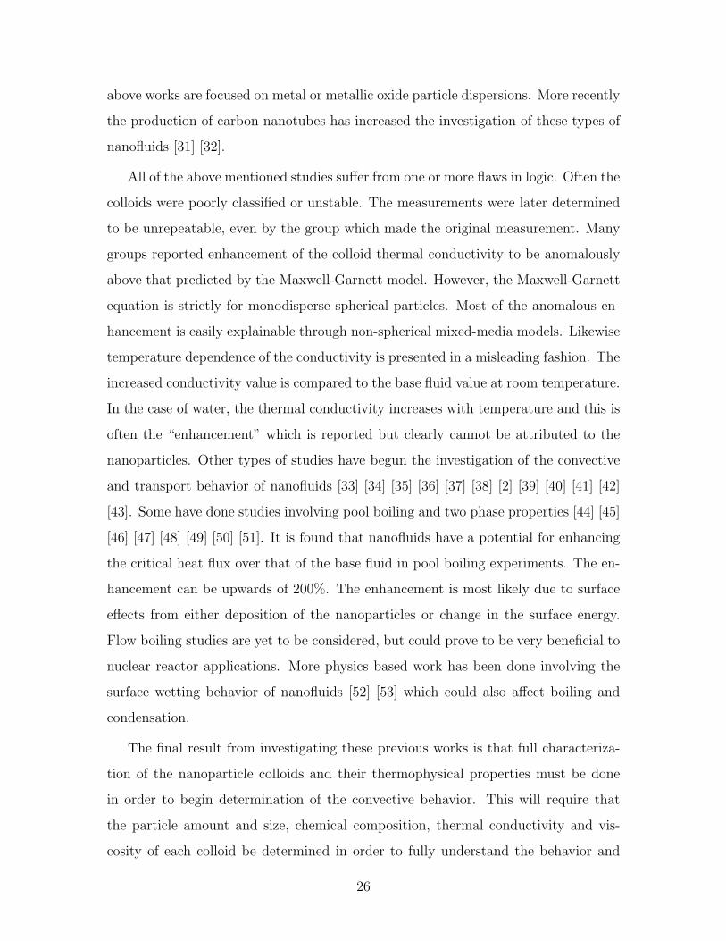
The final result from investigating these previous works is that full characteriza-
tion of the nanoparticle colloids and their thermophysical properties must be done
in order to begin determination of the convective behavior. This will require that
the particle amount and size, chemical composition, thermal conductivity and vis-
cosity of each colloid be determined in order to fully understand the behavior and
26

therefore model it. It can be seen that the promise of nanofluids as an effective way
to increase heat transfer capabilities of existing equipment opens a new horizon, not
unlike the material science revolution has for structural mechanics, where fluids can
be engineered in order to attain desired properties. This study has developed an
experimental apparatus and methodology which can be used to investigate the con-
vective heat transfer performance of nanoparticle colloids and shed more light on the
underlying phenomenology behind their behavior.
27

28

Chapter 2
Preparation and Characterization
of Nanofluids
The first step in studying nanofluids is their preparation and characterization. Only
well characterized fluids can be considered if one wants to limit the unknowns in
the experiments to be undertaken. It is also important to understand the behavior
of nanofluids from a fundamental point of view in order to best realize them in an
engineered system. An understanding of the preparation and characterization of a
nanofluid begins with introductory colloid and surface science. Insight is given to
some of the more complex issues of nanofluid characterization. Using this existing
knowledge as the basis, techniques for characterizing colloids are used to investigate
various nanofluids for potential use in the conductive and convective heat transfer
experiments.
2.1 Colloid and Surface Science
An introduction to colloid and surface science is essential to the understanding of
nanofluids. Some key definitions will be covered, followed by the ideas of colloidal
stability and the methods for achieving it. It is not the intention to repeat the
contents of the many existing books in the field, but to summarize them concisely for
the introductory nanofluid scientist.
29

2.1.1 Definitions
The following definitions are useful when discussing nanofluids (or colloids)[10]:
Solvent - The base fluid containing the nanoparticles
Dispersant, Particles, or Solute - Nanoparticles dispersed in the solvent
Colloid or Dispersion - A class of materials that exists between molecular and
bulk dispersion systems, where one of the solute dimensions is roughly between 1 and
1000 nm.
Laminated Dispersion - Dispersant with one dimension below 1000nm
Fibrillar Dispersion - Dispersant with two dimensions below 1000nm
Corpuscular Dispersion - Dispersant with three dimensions below 1000nm (most
nanofluids)
Lyophobic - Dispersant strongly repels solvent
Lyophillic - Dispersant strongly attracts solvent
Hydrophobic - Lyophobic to water
Hydrophillic - Lyophillic to water
Surfactant - A surface active agent which lowers the interfacial tension, surface
tension, or improves wettibility of a liquid
Monodisperse - Dispersion where all particles are relatively the same size
Polydisperse - Dispersion where particles have a range of sizes
Floc - An open, loosely connected grouping of particles (reversible)
Flocculation - the formation of flocs
Coagulum - A dense, strongly connected grouping of particles (not reversible)
Coagulation - the formation of coagulates
Sedimentation - the falling separation of flocs or coagulum to the bottom of the
dispersion (particles which are denser than the liquid)
Creaming - the floating separation of flocs or coagulum to the top of the dispersion
(particles which are less dense than the liquid)
Aggregates - Particles which have sedimented or creamed out of the dispersion
30

10 100 10000.00
0.05
0.10
0.15
0.20
0.25
0.30
Perc
ent (
%)
Particle Diameter (nm)
0.05nm3
0.1nm3
Figure 2-1: Percentage of molecules in the surface of particles depending on particlediameter for two characteristic molecular sizes
2.1.2 Surface Properties in Colloids
A key principle in dealing with colloids involves the notion of properties. It is seen
from simple analysis that the number of molecules in the particle surface relative to
the total molecules in the particle can be given by
Number fraction of particles ∼ 6(l/dp) (2.1)
where l is the characteristic length of the single molecule and dp is the particle charac-
teristic length (the diameter for a spherical particle). A plot of this ratio gives insight
into this property for nanofluids as shown in Figure 2-1. It is shown that below
∼100nm the number of molecules in the surface can become significant. The implica-
tions of this are that the surface molecules do not behave thermodynamically in the
same manner as the bulk material molecules. This is due to the interface between
the solid and liquid. In large materials the surface effect is relatively unimportant
in comparison to the bulk material present. In a small particle, the curvature and
surface to volume ratio would allow for a surface molecule to see the bulk material
on less than 50% of its sides. This can be seen conceptually in Figure 2-2. Material
properties are strictly dependent on the molecular interactions and it is hard to think
31

Molecule in the middleof bulk material
Surface moleculeon planar surface
Visualization of“potential”
Surface moleculeon curved surface
ParticleMolecule
LiquidMolecule
Figure 2-2: Visualization of surface molecules
of the particles as being thermodynamically homogenous. Also chemical reactions
that occur at the surface can be increased by this increase in surface accessible to
the fluid. Of these chemical effects the electrical double layer is of major importance
to colloidal stability. Free energy arises due to the differences of the intermolecular
forces “felt” by the molecules in the bulk material and those felt by the surface mole-
cules as shown in Figure 2-2. This can be seen from the free energy due to the surface
tension,
∆G = 2σAp (2.2)
where ∆G is the free energy, σ is the surface tension, and Ap is the surface area.
This free energy is due to the attraction of like molecules in the surface. Therefore
the minimization of free energy comes through minimization of surface area. For
this reason all particle surfaces will attract in both vacuum and in dispersion in an
attempt to minimize this surface area. The effect of solvent in this situation is to
slightly lower this attraction between surfaces due to the solvent/solute interaction
and surface tension of the fluid. In general, the solvent is not enough to prevent
flocculation and coagulation of the particles. Therefore all colloids are inherently
unstable due to this free energy of attraction. In order to prevent flocculation or
coagulation and hence achieve metastability or colloidal stability an energy barrier
must be created to prevent the close contact of particle surfaces with one another.
32

2.1.3 Colloidal Stability
As mentioned above, colloidal stability is achieved through the creation of an energy
barrier which would prevent the particles from coming in close proximity and thus
aggregating. The concept can be visualized as the total interparticle potential energy
of interaction curve. One can consider that the particles have multiple attractive and
repulsive forces. The forces create more free energies similar to those shown in the
previous section, where ∆Gatt would be the attractive and ∆Grep the repulsive free
energy of interaction. These forces are a function of the separation distance between
the particles. A summation of the forces would give a total interaction potential
curve. The creation of a local maximum in this curve would amount to a barrier and
thus create a metastable point. This can be seen relatively in Figure 2-3.
For spherical particles the attractive energy is found as
∆Gatt = −∆W =∫ ∞
dF attdr = −A
∫ ∞
d1/r7dr = −A′/d6 (2.3)
which is known as the London-van der Waals attraction, where A′ depends on the spe-
cific particle properties and d is the seperation distance. Likewise the Born repulsion
created by interaction of the electron clouds creates a repulsive energy of
∆Grep = (B/a)e−ad (2.4)
where a and B are constants. One can use an approximate expression
∆Grep = B′/d12 (2.5)
where B’ is a constant. Combination of these two terms into the total interaction
energy is
∆G = Grep + Gatt = (B′/d12)− (A′/d6) (2.6)
and is known as the Lennard-Jones potential. Of course this is overly simplified
if one is considering colloidal particles where electrostatic repulsion, steric repulsion,
33

and other effects come into play. For example if one considers the particles as charged
points then Coulomb’s law gives the electrostatic interaction force as
F el = q1q2/(4πε0d2) (2.7)
where q is the charge and ε0 is the dielectric constant. This force would give a
electrostatic repulsive energy of
∆Gel = q1q2/(4πε0d) (2.8)
measured relative to that at infinite separation. This term could be added to the
total interaction potential of Eq. 2.6 to give
∆G = Grep + Gatt + Gel = (B′/d12)− (A′/d6) + q1q2/(4πε0d) (2.9)
If the additional electrostatic or steric energies are designed properly one can create
an energy barrier which makes stable colloids.
The height of the energy barrier should be somewhat greater than kBT the thermal
energy of the liquid, where kB is the Boltzmann constant. This thermal energy of
the liquid is what creates the Brownian motion. Brownian motion is the only force
which can push the particle together over the energy barrier. Due to the probabilistic
nature of Brownian motion, usually a barrier of 10kBT is required to assure good
stability. Barrier height is dependent on fluid and particle composition, temperature,
and pressure. There are several methods for the creation of this energy barrier. Two
major methods will be discussed here: surface charging and surfactant adsorption.
The objective of these is to create repulsive forces to counteract the attraction of the
particle surfaces.
Surface charging is typically achieved with the electrical double layer. The simplest
way to visualize the double layer is as an ionic atmosphere around the particle which
is created by the chemical reaction between the solvent and the particle. The surface
of the particle will react with the solvent to create charged groups on the surface;
34

r
∆G AttractiveRepulsiveTotal
Barrier
Figure 2-3: Potential energy of interaction curves
this in turn builds the atmosphere of oppositely charged ions to balance the overall
charge. Conceptually the double layer is shown in Figure 2-4. The diffusive double
layer better visualizes the actual physics. The size and charge concentration of the
double layer directly affect the stability of colloids. The creation of like charges on the
surfaces of the particles makes a strong repulsive force between particles which falls
off exponentially as the interparticle distance is increased. This force is seen as the
barrier in the total interaction potential as shown in Figure 2-3. At long distances the
double layer covered particle would be seen as neutral, however when two particles
approach the interaction potentials overlap.
The common theory used to understand the force between charged surfaces inter-
acting through a liquid medium is known as DLVO theory, named after the developers
Derjaguin, Landau, Verwey, and Overbeek. This theory considers the Van der Waals
attraction and charged double layer repulsion between to particles in a vacuum or fluid
media. The theory also considers the charge screening due to the material between
35

Par
ticle
Par
ticle
HelmholtzModel
DiffusiveModel
Liqu
id
Liqu
id
Figure 2-4: Electrical Double Layer (Colors represent positively and negativelycharged ions
the particles. The potential is described as
U(r) =Z2e2
ε
[exp(κdp)
1 + κdp
]2exp(−κd)
d(2.10)
where ε is the dielectric constant of the liquid, d is the separation distance from center
to center of particle, dp is the sphere radius, Z is the number of electrons, e is the
electron charge and κ is the inverse of the Debye-Huckel screening length defined as
κ2 =4π
εkBT
∑α
nq2 (2.11)
where n is the concentration of simple ions of charge q.
However, DLVO theory is an approximation and does not consider non-continuum
effects which may be more prominent for short range particle interactions and dis-
persion interactions. Therefore the main assumption is that the particles are well
dispersed monosized spheres. Experimentally the interparticle potential is tradition-
ally understood through electrophoretic measurement and the zeta potential. More
recently atomic force microscopy (AFM) has been used for understanding these in-
teractions. The work of El Ghazaoui investigates both methods for the measurement
on alumina and zirconia double layer potentials [1]. Figures 2-5 and 2-6 show the
surface charge of zirconia and alumina for different pHs and concentration of NaCl.
36

Figure 2-5: Surface charge of crystalline zirconium dioxide as a function of the pHand the concentration of NaCl solution at 298 K [1].
37

Figure 2-6: Surface charge of α-alumina as a function of the pH and the concentrationof NaCl solution at 298 K [1].
38
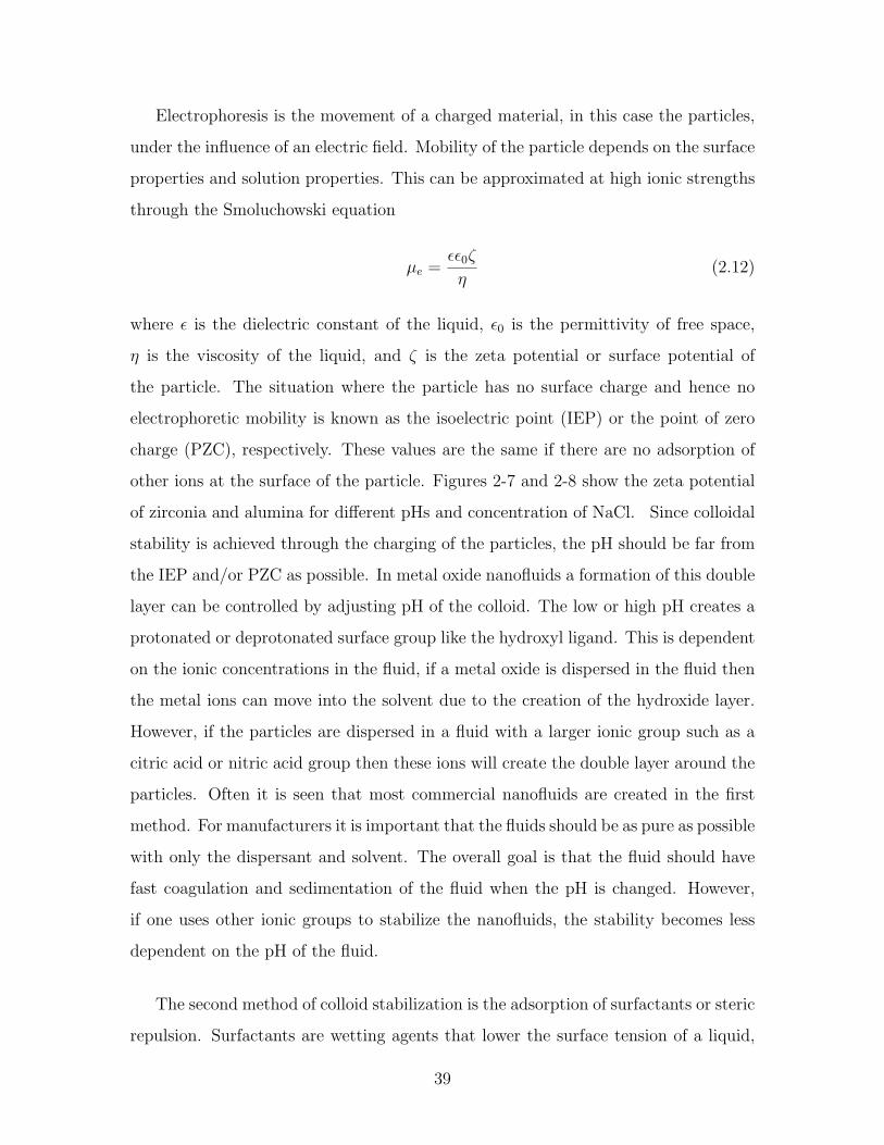
Electrophoresis is the movement of a charged material, in this case the particles,
under the influence of an electric field. Mobility of the particle depends on the surface
properties and solution properties. This can be approximated at high ionic strengths
through the Smoluchowski equation
µe =εε0ζ
η(2.12)
where ε is the dielectric constant of the liquid, ε0 is the permittivity of free space,
η is the viscosity of the liquid, and ζ is the zeta potential or surface potential of
the particle. The situation where the particle has no surface charge and hence no
electrophoretic mobility is known as the isoelectric point (IEP) or the point of zero
charge (PZC), respectively. These values are the same if there are no adsorption of
other ions at the surface of the particle. Figures 2-7 and 2-8 show the zeta potential
of zirconia and alumina for different pHs and concentration of NaCl. Since colloidal
stability is achieved through the charging of the particles, the pH should be far from
the IEP and/or PZC as possible. In metal oxide nanofluids a formation of this double
layer can be controlled by adjusting pH of the colloid. The low or high pH creates a
protonated or deprotonated surface group like the hydroxyl ligand. This is dependent
on the ionic concentrations in the fluid, if a metal oxide is dispersed in the fluid then
the metal ions can move into the solvent due to the creation of the hydroxide layer.
However, if the particles are dispersed in a fluid with a larger ionic group such as a
citric acid or nitric acid group then these ions will create the double layer around the
particles. Often it is seen that most commercial nanofluids are created in the first
method. For manufacturers it is important that the fluids should be as pure as possible
with only the dispersant and solvent. The overall goal is that the fluid should have
fast coagulation and sedimentation of the fluid when the pH is changed. However,
if one uses other ionic groups to stabilize the nanofluids, the stability becomes less
dependent on the pH of the fluid.
The second method of colloid stabilization is the adsorption of surfactants or steric
repulsion. Surfactants are wetting agents that lower the surface tension of a liquid,
39

Figure 2-7: Zeta potential of crystalline zirconium dioxide as a function of the pHand the concentration of NaCl solution at 298 K [1].
40

Figure 2-8: Zeta potential of α-alumina as a function of the pH and the concentrationof NaCl solution at 298 K [1].
41

r
∆G
Figure 2-9: Total interaction potential for steric repulsion
allowing easier spreading, and lower the interfacial tension between two liquids. They
can be seen simply as string-like materials with hydrophobic heads and hydrophillic
tails. The concept is similar to the double layer, except that the surfactants are
anchored to the surface and the tails of the surfactants reach out into the fluid. The
tails prevent the particles from approaching each other close enough to agglomerate.
The total interaction potential can be seen in Figure 2-9 and an illustration of the
technique in Figure 2-10.
Steric repulsion allows for more stability of a colloid under variable pH or concen-
tration conditions. However the adsorbed layers due to their organic nature have low
temperature and chemical resistance. It is often difficult to match the surfactants that
adhere to the particle and do not react with the solvent. It has been seen from other
works in the literature, like Krishnakumar [54], that steric repulsion stability can be
highly dependent on the dielectric constant of the fluid. The dielectric constant will
alter the amount of surfactant that can be adsorbed on the particle surface. The
amount of absorbtion determines the stability of the resultant colloid. It is therefore
very important to select the proper surfactant for the particular fluid/particle combi-
nation which often times requires trial and error. The work of Krisnakumar showed
42

ApproachingParticles
Minimum ApproachDistance
Par
ticle
Par
ticle
Par
ticle
Par
ticle
Surfactants
Figure 2-10: Conceptual image of steric repulsion
that Aerosol-OT (AOT) can effectively help to stabilize dispersions of alumina in
non-polar solvents, where surface charge stabilization is not possible.
2.1.4 Volume and mass fraction
In most all of the nanofluid thermal conductivity and heat transfer literature the par-
ticle loadings of the colloids are given in terms of volume fraction. Volume fraction is
desired in order to utilize the existing models for mixed media thermal conductivity
like the Maxwell-Garnett[8] or Hamilton-Crosser[7] models. However from an exper-
imental standpoint the exact volume fraction is quite difficult to determine. Due to
the large number of surface molecules in the particles, the macroscopic bulk material
density is not appropriate when calculating volume fraction. When the particles are
placed into solution the formation of oxide or other surface groups also changes the
volume being displaced by the particles.
Amorphous surfaces like the hydroxide layers on the outside of the particles can
be more porous, than the inner bulk material thus altering the effective volume as
well. Due to these chemical effects it is not possible to directly use weight and
density measurements in order to determine volume fraction. If one looks at the
43

mixed media thermal conductivity models, it is found that the resulting conductivity
is highly dependent on the volume fraction of the material. It is the author’s belief
that some of the discrepancies of the measured experimental values and the values
predicted by the models could be partially attributed to this effect. The adsorbed ion
layer effectively dilates the outer layers of the particle and hence increases its volume,
the outer layers thus becoming less dense. The models are strictly volume based.
Most studies are using the weight loading and density of the respective materials
in order to determine the volume loading for the modeling. This work follows the
same trend as the previous works, however regard is taken to the fact that volume
fraction can be misleading and that what might appear to be an anomalous change in
properties is potentially explainable through this effect. It however has no bearing on
the validity of the experimental results under flow conditions, if one realizes that the
properties are only interpreted through the weight fractions. Therefore the loadings
in the loop are compared directly with the properties of the samples taken from the
loop and the reference to volume fraction is the same as a reference to weight fraction
divided by the respective bulk density of the particle material.
Another interesting phenomenon is the alteration of the volume fraction of the col-
loid by changing the temperature. The density (volume) of some liquids is strongly
dependent on the temperature. The volume and hence density of the solid particles
is usually much less dependent on the temperature. For this reason one must con-
sider the fact that volume loading of a colloid actually can decrease as the system
is heated up. This temperature effect should be accounted for if one wants to use
volume averaging models to predict conductivity. There are other effects due to the
temperature which will be described in the next section. Once again this effect comes
out of the analysis of the flow situation due to the comparison with the exact samples
taken from the loop.
Finally, one study has mentioned that there is a potential to have liquid layering
at the surface of the particles and how this would affect the modeling of thermal
conductivity using volume weighting [28]. Molecular dynamics modeling of nanofluids
has shown that this liquid layering is not a structure but more like an ordered higher
44

density region created by the strong particle/fluid interaction, see the work of Eapen
[55]. Eapen showed this region could also potentially have higher thermal conductivity
due to other energy transport pathways, i.e. potential energy flux. This molecular
dynamics view fits closely with the concept of the interfacial shell model.
2.1.5 Temperature effects
Temperature can have some minor effects on nanofluid behavior beyond the simple
density effect discussed above. Due to the chemical nature of the double layer there
is a mild sensitivity to temperature change. The approximate thickness of the double
layer can be seen from the reciprocal of the Debye-Huckel parameter
κ−1 =√
ε0εrkBT/2NAe2fI (2.13)
where I is the ionic strength, NA is Avogadro’s number, ε0 is the permittivity of free
space, εr is the permittivity of the solution, T is the temperature and ef is the Faraday
constant. The change in the charge density, which is due to the change in the Debye-
Huckel parameter, can alter the stability of the nanofluid as well as the apparent
volume of the particles from a hydrodynamic viewpoint. This is a combined effect
with the increase in Brownian motion due to the temperature change which would
allow a slightly larger percentage of particles to “jump” the total potential barrier.
The ionic strength and permittivity is also affected by the temperature change. It
might be possible for an increase in temperature to destabilize a colloids because
the increase in the Brownian motion causes more jumping and the increase in Debye
Length effectively lowers the charge density around the particles if they are in the
same chemical equilibrium state. Likewise, surfactant hydrophilia can increase or
decrease with temperature as well. Therefore the change of temperature could create
a more or a less stable fluid. However it is typical that these effects are minimal and
most likely would not effect the fluid over moderate temperature ranges.
45

2.2 Preparation or purchase of nanofluids
Three main types of nanofluids are studied here: those made from purchased powders
mixed with water, those made from chemical precipitation in the liquid, and those
which are purchased. Other methods for the creation of nanofluids exist, i.e. plasma
arch deposition; but have not been studied in this project. It is very important
to understand fully the constituents of any nanofluid under investigation in order to
draw significant conclusions as to the heat transfer phenomena. It is common practice
to add various chemicals or surfactants in order to maintain nanofluid stability and
size distribution. These additional chemicals could also play an important role in
the transport phenomena as well as the potential to be used in the nuclear reactor
environment.
2.2.1 Preparation
The first attempt to make nanofluids consisted in purchasing nanoparticle powders
available from Sigma-Aldrich, see Tables 2.1 and 2.2, and mixing them with a base
fluid. Since the purity of the nanofluid is important, attempts were made to mix the
particles directly with water with no additives. The metallic oxide nanopowders are
not chemically reactive in atmosphere; however they do tend to form loose micro-sized
agglomerates in atmosphere and in fluid suspension over time. The most effective
method of breaking and evenly dispersing the powder in a fluid is through application
of ultrasonic vibration. It has been previously observed, by Das et al.[22], that this
technique will maintain fluids with less than 2% volume of particles in suspension
indefinitely and suspensions up to 4% by volume with only minor sedimentation.
The ultrasonic vibration was done for over 12 hours for each fluid by Das et al. with
effective results.
Using this methodology the nanofluids were created using the two oxide nanopow-
ders and ultrasonic vibration was applied for 12+ hours. The resulting nanofluids
initially looked promising, but were not stable for longer periods of time. Although
some particles remained dispersed, the majority formed larger agglomerates and set-
46

Table 2.1: Sigma-Aldrich Zirconium(IV) oxide nanopowder (www.sigmaaldrich.com)
tled out of the liquid. It is mentioned in the work of Das et al. that due to the short
duration of their testing, stabilizing agents such as surfactants or pH control were
not used. It is believed that the cause of the differences in stabilities of our nanoflu-
ids and those of Das et al. could either be due to poor sonication of our samples
or nanoparticles from Nanophase Technology Corporation are better dispersed than
those from Sigma-Aldrich. This remains to be verified.
As stated earlier, the small particle size gives the potential for the particle to
escape settling due to gravity. The Brownian motion of the fluid keeps the particles
aloft. However this small particle size dramatically increases the surface to volume
ratio of the system. In order to increase the surface area of a material energy must be
input into the system. This energy is input by breaking and dispersing the particles.
Standard methods for breaking and dispersing are high speed stirring, ball milling,
ultrasonication, and high shear nozzles. Therefore the distance from the point of
energy stability is increased by increasing the surface area of the particles with these
methods. The fully suspended system is either unstable or metastable at best, as
found in colloid and surface science.
The other method for creating nanofluids tried in this study is through chem-
ical precipitation with the addition of surfactants. It is theoretically possible to
47

Table 2.2: Sigma-Aldrich Aluminum oxide nanopowder (www.sigmaaldrich.com)
48

make any metal oxide nanofluid in this manner. Making of the Fe3O4 nanofluid is
described as follows: To begin, excess oxygen is removed from deionized water by
bubbling through nitrogen. Then, a 1:2 molar ratio of Iron (II) Chloride Tetrahy-
drate (FeCl2·4H2O) and Iron (III) Chloride Hexahydrate (FeCl3·6H2O) are added to
the water. The mixture is stirred and heated to 80C and becomes yellowish in color.
Next, the polymer/surfactant Poly(4-styrenesulfonic acid-co-maleic acid) sodium salt
[CH2CH(C6H4SO3R)]x[CH(CO2R)CH(CO2R)]y, (where R = H or Na) is added to
the mixture until it is foaming.
In order to precipitate the particles a solution of Ammonium Hydroxide ∼28% is
added and the solution immediately turns black with the iron oxide nanoparticles.
The nanometer size of the particles is created due to the equilibrium between the
amount of materials in the mixture. The quick adsorption of polymer surfactant on
the particle surfaces is what prevents them from growing into larger macro particles.
This solution is allowed to stir and fully react at 80C for 30 minutes. The resulting
nanoparticles are cleaned with acetone and separated from the liquid by using an
electromagnet (particles are magnetite). If particles were not magnetic i.e. Al2O3
or ZrO2, then centrifuging could be used. The cleaning process is repeated with
deionized water, acetone, and the magnet several more times. The final particles are
then heated to boil off the excess acetone and can then be dispersed in water. The
final dispersion has been found to be stable indefinitely.
2.2.2 Purchase
Purchase of nanofluids has become more prevalent and cost effective over the past few
years. Several companies list nanofluids as products. However it has been found, as
will be shown later, that some contain overly contaminated products or products that
do not meet specifications. Several companies were approached for samples in this
project: Nyacol, Sigma-Aldrich, Nanophase Technologies, Applied Nanoworks and
Meliorum Technologies, to name a few. These companies produce many nanofluid
products with varying quality. The major candidates for this project which are pur-
chased are water-based with zirconia and alumina particles, however some other fluids
49

have also been investigated.
2.3 Characterization
As stated above, it is important to be able to fully characterize the nanofluids under
inspection for heat transfer enhancement. The first steps are to quantify the com-
position, size and loading of the nanoparticles, pH, and search for impurities in the
nanofluids. Methods for finding these experimentally are discussed along with the
results of these experiments.
2.3.1 Characterization methods
Some common tools are utilized to characterize and qualify nanofluids these include:
neutron activation analysis (NAA), inductively-coupled plasma spectroscopy (ICP),
transmission electron microscopy (TEM) imaging, thermogravimetric analysis (TGA)
and dynamic light scattering (DLS). These will be described below.
Transmission electron microscopy (TEM)
TEM is the primary technique to verify single particle dimensions and to identify
agglomerations of particles. The electron beam can be used to see features on the
nanometer level. A major drawback to the use of TEM is that samples must be
dried out of solution in order to be attached to the carbon matrix and placed in the
vacuum chamber of the TEM; therefore the particles are not exactly in the colloid
state and agglomeration might occur during drying. However, TEM can be used in
combination with dynamic light scattering to acquire exact sizing in nanofluid form.
Another drawback of TEM is the cost and time investment needed to prepare
and view the sample. It was decided that only some initial imaging will be done
as a feasibility study. Later dynamic light scattering, which is a much simpler and
less time consuming technique, will be used to first quantify the nanofluids and then
selected samples will be viewed with the TEM. An example of one of the nanofluids
(Sigma-Aldrich Al2O3 in water) can be seen in Figure 2-11. As seen in Figure 2-11
50

Figure 2-11: TEM image of Sigma-Aldrich Al2O3 nanofluid
the smallest particles are on the order of 40-50nm and are slightly oblong in shape.
The larger loose agglomerations of particles are in the 250nm range. The time of
agglomeration cannot be told from the images and may have occurred during the
drying process on the slide. The mean particle size appears to be in agreement with
the specifications of Sigma-Aldrich. It is therefore shown that TEM is a useful tool
for particle sizing, but has limitations as discussed above.
Dynamic light scattering (DLS)
The dynamic light scattering technique used in this work is described in the work of
Kim [56] as follows:
Dynamic light scattering (DLS) theory is a well established technique
for measuring particle size over the size range from a few nanometers
to a few microns. The concept uses the idea that small particles in a
suspension move in a random pattern. A microbiologist by the name of
Brown first discovered this effect while observing objects thought to be
living organisms, by light microscopy. Later it was determined that the
”organisms” were actually particles, but the term has endured. Thus,
51

the movement of small particles in a resting fluid is termed ”Brownian
Motion” and can easily be observed for particles of approximately 0.5
to 1.0 microns bounce a microscope at a magnification of 200 to 400X.
Observation of larger particles compared to smaller particles will show
that the larger particles move more slowly than the smaller ones given the
same temperature. According to Einstein’s developments in his Kinetic
Molecular Theory, molecules that are much smaller than the particles
can impart a change to the direction of the particle and its velocity. Thus
water molecules (0.00033 microns) can move polystyrene particles as large
as a couple of microns. The combination of these effects is observed as an
overall random motion of the particle.
When a coherent source of light such as a laser having a known frequency
is directed at the moving particles, the light is scattered, but at a different
frequency. The change in the frequency is quite similar to the change in
frequency or pitch one hears when an ambulance with its wailing siren
approaches and finally passes. The shift is termed a Doppler shift or
broadening, and the concept is the same for light when it interacts with
small moving particles. For the purposes of particle measurement, the
shift in light frequency is related to the size of the particles causing the
shift. Due to their average velocity, smaller particles cause a greater shift
in the light frequency than larger particles. Thus, the difference in the
frequency of the scattered light among particles of different sizes is used
to determine the sizes of the particles present.
The DLS equipment used for this study consists of mainly three compo-
nents. A laser purchased from Spectra-Physics emits a 514 nm wavelength
of argon. A goniometer from Brookhaven preserves any scattering between
the incident laser and present nano-size particle, which is placed onto a
bath. Finally, a detector from Brookhaven detects a laser scattered in 90
degrees from the incident laser since the angle between the goniometer
52

Figure 2-12: Schematic Diagram of light scattering measurement with a dynamicmode
and detector is fixed as 90 degrees. This configuration is well reflected
in the Figure 2-12. It is of importance to clarify the physical situation
upon this scattering measurement. Since the expected particle size will
be smaller than the wavelength of the incident laser, this kind of scatter-
ing can be categorized as the Rayleigh scattering, which is defined as the
scattering of light, or other electromagnetic radiation, by particles much
smaller than the wavelength of the light.
In addition, an alternative mode of light scattering measurement, static
light scattering, is also viable if the configuration allows the goniometer
to rotate automatically. In such a case, scattered lasers will be detected
according to the angle change, which gives the angular distribution of
particle size. In either modes of dynamic or static, hydrodynamic or
53

gyration particle sizes can be obtained, respectively. When we measure a
particle size, in practice, it is necessary to start with several assumptions.
First the particles can be assumed to be in Brownian motion. Second, it
assumed that the particle do not interact with each other. In a practical
measurement, the second assumption can be valid when the fluid contains
a small number of particles. With those assumptions, the average motion
of a particle can be described by using an intermediate scattering function
f(q, τ) = exp[−ip(r(0)− r(τ)] = exp(iq∆r(τ)) (2.14)
where p = (4π/λ)sin(θ/2) is a scattering factor, λ is a wavelength of
scattered light, θ is an angle between incident and scattered lights, τ is the
time scale during the scattering, and ∆r(t) = r(t)− r(0) is displacement
of particle in time t. For particles in Brownian motion, ∆r(t) is a real 3-D
Gaussian variable and therefore f(q, τ) and the mean square displacement
< ∆r2(t) > becomes
f(q, τ) = exp
[−q2
6< ∆r2(t) >
](2.15)
and
< ∆r2(t) >= 6D0τ (2.16)
which when combined form
f(q, τ) = exp[−q2D0τ
](2.17)
where D0 is the mass diffusion constant defined by the Stokes-Einstein
theory as
D0 =kBT
6πηdp
(2.18)
where η is the viscosity of the fluid and R is the radius of the particle. In
the measurement, the measured quantity is the diffusion constant based
54

Figure 2-13: DLS analysis of Sigma-Aldrich Al2O3 nanofluid (d is particle diameterand G(d) is the intensity of the light)
on the known applied power and time. Using the obtained f(q, t), from
which it is viable to induce the diffusion constant by a simple algebra to
determine the radius of the particle. It should be noted that this is the
Stokes or hydrodynamic radius of the particle. This radius can differ from
the actual radius due to the surface charging, as described above.
An example of the raw output for Sigma-Aldrich Al2O3 nanofluid measured with
DLS is shown in Figure 2-13. It can be seen that the majority of the intensity
is around the 200nm sizing, but there are some counts at the ∼40nm size. This
seems to be in good comparison to the results of the TEM imaging. However one of
the main drawbacks of DLS is the measurement of very polydisperse systems. The
intensity of the light scattered increases with the diameter of the particle. Therefore
the sizes measured are correct, but the distribution of the particles in these size
bins needs to be weighted according to their diameters. If this is corrected for in
the analysis (which is automatically done by the software), then the majority of the
55

Figure 2-14: DLS analysis of Sigma-Aldrich Al2O3 nanofluid after correction
particles are in the 40nm range with a few larger agglomerations, see Figure 2-14,
which reinforces previous findings and the technical specifications of the fluid. The
pH of the Sigma-Aldrich is around 4 in order to maintain the particles in dispersion.
If the pH is allowed to rise to 7, the agglomerations are seen to increase significantly.
Therefore care must be taken to maintain the nanofluid pH stable during dilution for
the DLS measurement, this will be shown later. Other DLS measurements are made
on Nyacol alumina and zirconia, see Figures 2-15 and 2-16 and the Fe3O4 nanofluids
with reasonable results. It has been determined that DLS is an effective way of
determining nanofluid particle sizes in solution and in combination with TEM, full
characterization of particles sizes and distributions is possible.
56

Figure 2-15: DLS analysis of Nyacol Al2O3 nanofluid
Figure 2-16: DLS analysis of Nyacol ZrO2 nanofluid after correction)
57

Table 2.3: Elements detectible by neutron activation analysisAluminum Dysprosium Lanthanum Potassium TelluriumAntimony Erbium Lutetium Praseodymium TerbiumArsenic Europium Magnesium Rhenium ThoriumBarium Gadolinium Manganese Rubidium ThuliumBromine Gallium Mercury Ruthenium ZirconiumTin Cadmium Germanium Molybdenum SamariumTitanium Cerium Gold Neodymium ScandiumTungsten Cesium Hafnium Nickel SeleniumUranium Chlorine Indium Niobium SilverVanadium Chromium Iodine Osmium SodiumYtterbium Cobalt Iridium Palladium StrontiumZinc Copper Iron Platinum Tantalum
Neutron activation analysis (NAA)
Particle concentration in the nanofluid solution is another problem of characteriza-
tion. The capabilities of MIT’s research reactor to perform neutron activation analy-
sis are utilized for determining nanoparticle and other impurity concentrations in the
nanofluids. NAA is a method that uses the gamma decay emissions of the samples
after having undergone neutron irradiation to identify elements and their concentra-
tions. Irradiation times depend on the materials under investigation and the half life
of the gamma decay modes. Table 2.3 lists all of the elements detectible using NAA.
Two zirconia nanofluid samples are irradiated, because of the long zirconium half life
the samples have been irradiated for 6 hours. Both samples are supplied as 10 percent
zirconia by weight in water from the vendors. Samples are from Sigma-Aldrich and
Applied Nanoworks. The measurements were conducted by experienced NRL staff,
so the details will not be reported here. The results found that both nanofluids con-
tained zirconium, 0.076gm/gm in the Sigma-Aldrich and 0.0203gm/gm in the Applied
Nanoworks. In order to determine the amount of zirconia, it is assumed all of the zir-
conium is in the form of the oxide and contains two oxygen atoms. By addition of this
extra weight it is found that the Sigma-Aldrich has 0.1027gm/gm or 10.27wt% zirco-
nia and the Applied Nanoworks has 0.0274gm/gm or 2.74wt% zirconia. Therefore it
is concluded that the Sigma-Aldrich is very close to the manufacturer specifications;
58

the Applied Nanoworks is dramatically different than the specifications.
Also, there is as much zinc as zirconium in the Applied Nanoworks sample; the
zinc has been found at 2.6wt%, which is a significant contamination. The Sigma-
Aldrich sample only has 6.5e-3wt%, which is insignificant. It is believed that the
Applied Nanoworks specifications are either unreliable or that the batch is overly
contaminated. Trace amounts (ppm levels) of other elements (K, Cl, Na) are found
and assumed to be as additives for pH control or just in the water used for dispersion.
Some alumina nanofluids have also been considered. Nyacol at 20wt% (NY),
Meliorum (ML) and Sigma-Aldrich (SA) at 10wt% were the three measured fluids.
For the alumina both short and long irradiations are required. The long (6 hours) is
for the majority of elements and the short (5 mins) is for the aluminum due to the
short half life. The results of the long show that the samples all contained nearly
insignificant levels (ppm) of Na, K, and a few other earth elements like Zn.
The results of the short irradiations gave the loading of the aluminum and thus
alumina for the nanofluids. It is seen that the NY has 19.37wt%, specs gave 20wt%.
The ML has 9.74wt% and the SA has 8.68wt% for 10wt% in the specs. These seem to
be in good agreement with the specifications of the vendors. The discrepancy of the
SA is assumed to be due to settling of the nanofluid, because it was an older sample.
Further tests would be required to make certain that the SA discrepancy was due to
settling. It is concluded that NAA can be used for quality control of nanofluids. The
major limiting factors of NAA is the time and cost of the procedure. It also involves
handling of radioactive materials.
Inductively-coupled plasma spectroscopy (ICP)
A more cost and time effective approach has been selected for determining the nanopar-
ticle loading and composition, i.e., the ICP spectrometer. ICP spectrometry uses the
light spectrum released from injecting materials into an extremely high temperature
plasma. The list of elements detectible by ICP is listed in Table 2.4. In general the
sensitivity of the ICP is lower than that of the NAA.
Each sample analysis takes only a few minutes once the ICP is calibrated for the
59

Table 2.4: Elements detectible by ICPAr Ca Eu In Na S Ta YAg Cd Fe K Nb Sb Th YbAl Ce Ga La Nd Sc Ti ZnAs Co Gd Li Ni Se Tl ZrB Cr Ge Lu P Si Tm BaCu Hf Mg Pb Sm U Be DyHg Mn Pr Sn V Bi Er HoMo Re Sr W - - - -
element of interest. Two samples are tested using the ICP: Al2O3 (Sigma-Aldrich)
and Fe3O4 in water. One key to the analysis is that the nanofluid samples need to
be diluted to stay below the maximum concentration of the calibration standards.
Therefore the Al2O3 which was initially at 10wt% is diluted to 0.05wt% (200:1) and
the Fe3O4 which was initially at 3.5wt% (polymer & iron oxide) is diluted to 0.035wt%
(100:1), both using deionized water. The Al2O3 is found to be at a concentration of
0.047wt% which is within ∼5% of the specified value. This is somewhat closer result
than that from the NAA. Sodium and potassium are also found, which is consistent
with the NAA results. These are used to stabilize the nanofluid using the pH method.
The Fe3O4 is seen to have a concentration of 0.034wt% which is within ∼10% of the
specified value (∼0.031wt%). The sodium of the stabilizing polymer could also be
seen by the ICP. These results are determined to be valid. The advantage of ICP
is its speed. It is more accurate than the NAA with respect to the alumina sample.
However, the nanoparticles may not be effectively introduced in the nebulizer if large
agglomerations occur. Therefore care must be taken to prevent agglomeration when
diluting pH stabilized nanofluids.
Thermogravimetric analysis (TGA)
Thermogravimetric analysis of nanofluids provides another means of analyzing differ-
ent components of a nanofluid by weight. This may be desirable when one needs to
know an accurate weight percentage of nanoparticles in solvent, or when the amount of
polymer (added to improve the nanoparticle stability) in a nanofluid must be known.
60

50 100 150 200 250 300
0
20
40
60
80
100
3.5%3.06%
Wei
ght P
erce
ntag
e
Temperature (oC)
Figure 2-17: Thermal gravimetric analysis of Fe3O4 nanofluid in water with surfac-tants
Thermogravimetric analysis works by heating a small sample on an extremely sen-
sitive balance in a high temperature furnace. The weight vs time curve combined
with knowledge of the boiling point of the species in the samples provide the sample
composition. The specific equipment to be used is the Perkin Elmer TGA7. Samples,
typically less than 40mg, are placed on a platinum balance and can be heated to over
1000C.
Figure 2-17 shows outputs from the TGA7 for the Fe3O4 nanofluid produced.
Weight percentage remaining is plotted on the y-axis, with temperature on the x-axis.
The polymer poly(4-styrenesulfonic acid-co-maleic acid) did not completely “cook
off” until higher temperatures, around 300C or 400C. Results have shown that this
polymer, by weight, makes up about 12% of the polymer coated Fe3O4 nanoparticles,
whereas the rest is composed of Fe3O4. The weight loading of a nanofluid can easily
be determined in this fashion, 3.5wt% for the iron oxide plus surfactant and 3.06wt%
for the iron oxide alone. A sample of the Nyacol Al2O3 nanofluid was also tested at
20wt%. The results of the TGA showed that the particles consisted of 21.8wt%, which
is slightly higher than the specified value. However further heating to the maximum
temperature found that the alumina is at 20.070wt%. It is believed that this extra
61

weight could possibly be due to the left over hydroxide groups on the surface of the
particles.
TGA has been found to be a simple way of measuring particle loading in nanoflu-
ids. It is inexpensive and uses very little of the sample. However it is not obvious
what constituents are producing the final weight results. If the nanofluids have se-
vere contamination, this could be incorrectly seen as additional particles in the final
weight loading. It is therefore intelligent to use both the ICP and TGA in order to
fully understand the loading of the nanofluid.
KD2 thermal conductivity analyzer
An important property to be characterized in this study is the thermal conductivity of
the nanofluid. In order to select the desired fluids to be fully characterized, enhanced
thermal conductivity is possibly the most important element in this study, because
it points to the nanofluid with high heat transfer potential. There is an inexpensive
commercially available system for the measurement of the thermal conductivity. The
Decagon Devices KD2 thermal properties analyzer, after some initial testing, is used
on all nanofluids at room temperature as a first check. In later sections, the transient
hot wire method, on which the KD2 operates, will be described in full along with the
true thermal conductivity measurement apparatus.
The accuracy of the KD2 is given as 5% by the manufacturer over a span of
temperatures of 0 to 60C. However it is found, through trial and error, that the KD2
operates very accurately if the probe is setup perfectly vertical and an isothermal bath
is used to maintain the sample at 25C. These measures prevent convection problems
and the external boundary effect problems. A schematic of the KD2 setup with the
isothermal bath is shown in Figure 2-18.
In order to test the accuracy of the KD2, mixtures of water and ethylene glycol
are prepared and tested against existing data in the literature from Bohne, Fischer,
and Obermeier [57]. The results of the measurement are shown in Figure 2-19. It can
be seen that the KD2 is quite accurate in measuring the values of the mixtures. This
is a reassurance of the KD2’s operation and it is therefore acceptable as an initial
62

0.60
III
ConstantTemperature
Bath
KD2 Probe
Fluid Sample
50mL Glass Tube
Lab Stand
Lab Stand
KD2
KD2
ConstantTemperature
Bath
TOP VIEW
SIDE VIEW
Figure 2-18: Schematic setup of KD2 thermal properties analyzer
63

0.0 0.2 0.4 0.6 0.8 1.00.20
0.25
0.30
0.35
0.40
0.45
0.50
0.55
0.60
0.65Th
erm
al C
ondu
ctiv
ity (W
/m-K
)
Mass Fraction of Ethylene Glycol in Water
Bohne, Fisher, & Obermeir (1984) KD2 Measurement
Figure 2-19: Thermal conductivity of water and ethylene glycol mixtures
scoping tool for thermal conductivity.
2.3.2 Experimental selection of nanofluid samples
Using the characterization techniques as described above many nanofluids have been
tested as potential candidates for further experimental investigation. The key prop-
erties used as criteria to eliminate the bad candidates are thermal conductivity en-
hancement, stability, and contamination.
Thermal conductivity at room temperature
Initially both water and ethylene glycol nanofluids are considered due to the availabil-
ity of the data in the literature for these fluids. It has been previously decided that
64

the scope of this work would be limited to water based nanofluids. The measured
thermal conductivity at room temperature for the nanofluids can be seen in Table 2.5
along with the loadings, manufacturers, and measured pH values. It is seen that few
fluids have enhancement in the conductivity and none of the fluids have what would
be considered anomalous enhancement beyond that of the mixed media model, like
Maxwell-Garnett, as shown. From this list, a short list of good candidates is compiled
which includes primarily alumina in water fluids from Sigma-Aldrich, Meliorum, and
Nyacol. Secondary candidates are zirconia in water fluids from Sigma-Aldrich and Ny-
acol, diamond in water fluid from the University of Florida and Applied Nanoworks,
silica in water fluid from Applied Nanoworks. Due to time constraints only the Nyacol
Alumina and Zirconia are selected for the full experiments.
Investigation of colloidal stability
Further investigation of the Nyacol and Sigma-Aldrich alumina is done because of
alumina nanofluid being of primary interest for the experiments. Some of the colloidal
stability properties can be easily shown experimentally with particle sizing techniques.
A small experiment on the size/stability of oxide particles with pH was done. Two
loadings of alumina are created from 10% by weight alumina in water nanofluids from
Sigma-Aldrich and another two from 20% by weight. The Sigma-Aldrich fluid has
a pH value of 4.3, thus during dilution with water the pH was allowed to change
towards neutral. The size and stability effects are highly visible using dynamic light
scattering. The initial Sigma-Aldrich fluid is shown in Figure 2-20 where the mean
diameter is 51.32nm with some minor flocs at higher diameters. The samples are
diluted to 0.01% and 0.001% by weight and allowed to sit for 1 hour. It can be
seen in Figures 2-21 and 2-22 that the mean diameter has increased to 90.09nm and
181.15nm, respectively.
The samples are then allowed to sit for 1 day. It can be seen in Figures 2-23
and 2-24 the mean diameter has increased to 129.02nm and 224.51nm, respectively
for 0.01%wt and 0.001%wt. The pH change due to dilution is a very important
parameter to the overall size and stability of the nanofluid. This was predictable
65

Table 2.5: List of samples which have been investigated for thermal conductivityenhancement
Particle Liquid Maker Preparation pHwt% vol% Measured Predicted
EG 0.25 0.25Ag EG MIT No Surfact/No pH 0.029 - - 0.25 0.25Al2O3 EG MIT No Surfact/No pH - ~3 8.5 0.28 0.27Au EG Meliorum Surfactants - 1 - 0.25 0.26CuO EG MIT No Surfact/No pH - ~1 4.15 0.27 0.26SiO2 EG MIT No Surfact/No pH - 1.6-3.3 - 0.28 0.26ZrO2 EG MIT No Surfact/No pH - 4 - 0.28 0.27
H 2 O 0.59 0.59
Al2O3 H2O SA pH 10 - 4.3 0.63 0.64Al2O3 H2O RPI Surfactants - 2 (0.5) 8.15 (7.05) 0.64 (0.62) 0.63 (0.60)Al2O3 H2O Nyacol pH 20 - 4 0.68 0.70Al2O3 H2O Meliorum pH 10 - 3.9 0.62 0.64Au H2O Meliorum Surfactants - 5 - 0.58 0.68Cu H2O MIT No Surfact/No pH - 0.5 6.5 0.59 0.60CuO H2O MIT No Surfact/No pH - <5 7.12 0.59 0.61Diamond H2O UF No Surfact/No pH 1.7 - 6.67 0.62 0.60Diamond H2O MIT No Surfact/No pH 0.1 - 6 0.60 0.59Fe3O4 H2O MIT Polymer Surfactant - 1 8.54 0.56 0.60Pt H2O Meliorum ? 0.0486 - - 0.57 0.59SiO2 H2O Applied Nano pH 10 - 10.17 0.63 0.62SiO2 H2O Polimi ? 34 18.6 7.13 0.63 0.69SiO2 H2O MIT No Surfact/No pH 5 - - 0.57 0.60Teflon H2O Polimi No Surfact/No pH 10.2 5 3.35 0.58 0.57ZnO2 H2O MIT No Surfact/No pH - 0.4 7.15 0.59 0.59ZrO2 H2O SA pH 10 - 2.7 0.62 0.60ZrO2 H2O MIT No Surfact/No pH 17 4 5.27 0.62 0.62ZrO2 H2O Applied Nano pH 10 - 4.17 0.59 0.60ZrO2 H2O Nyacol pH 20 - 4.17 0.61 0.62
Loading Conductivity
66
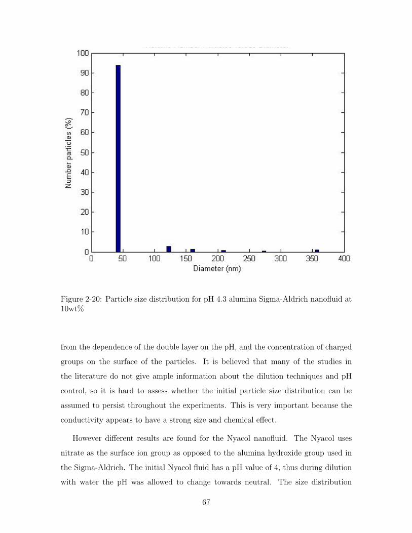
Figure 2-20: Particle size distribution for pH 4.3 alumina Sigma-Aldrich nanofluid at10wt%
from the dependence of the double layer on the pH, and the concentration of charged
groups on the surface of the particles. It is believed that many of the studies in
the literature do not give ample information about the dilution techniques and pH
control, so it is hard to assess whether the initial particle size distribution can be
assumed to persist throughout the experiments. This is very important because the
conductivity appears to have a strong size and chemical effect.
However different results are found for the Nyacol nanofluid. The Nyacol uses
nitrate as the surface ion group as opposed to the alumina hydroxide group used in
the Sigma-Aldrich. The initial Nyacol fluid has a pH value of 4, thus during dilution
with water the pH was allowed to change towards neutral. The size distribution
67

Figure 2-21: Particle size distribution for 0.01%wt alumina Sigma-Aldrich nanofluidat one hour
68

Figure 2-22: Particle size distribution for 0.001%wt alumina Sigma-Aldrich nanofluidat one hour
69

Figure 2-23: Particle size distribution for 0.01%wt alumina Sigma-Aldrich nanofluidat one day
70

Figure 2-24: Particle size distribution for 0.001%wt alumina Sigma-Aldrich nanofluidat one day
71

is shown in Figure 2-25 where the mean diameter is 37.8nm with some minor flocs
at higher diameters. The samples are diluted to 0.04% and 0.004% by weight and
allowed to sit for 1 hour. It can be seen in Figures 2-26 and 2-27 the mean diameter
has increased slightly to 42.6nm and 52.3nm, respectively. The samples were then
allowed to sit for 1 day. It can be seen in Figures 2-28 and 2-29 the mean diameter is
basically unchanged at 46.7nm and 46.7nm, respectively for 0.04%wt and 0.004%wt.
The pH change due to dilution is less important for the nitrate stabilized nanofluid.
Salt concentration plays an important role in the double layer size and strength.
Because the size distribution of its particles is not strongly affected by dilution the
use of Nyacol nanofluid should be easier in an engineering system. For this reason
the Nyacol nanofluids (alumina and zirconia) were the final selections to be used in
the experimental loop.
2.3.3 Conclusions
In conclusion, there are many variables that must be accounted for when dealing
with nanofluid (colloid) experiments. The conceptual and theoretical developments
of colloid and surface science lead to a far better understanding of nanofluid prop-
erties and behavior. Some properties such as size and stability are easily altered by
concentration, pH, and temperature modifications.
It is determined that nanofluids can be purchased or made in a variety of ways.
Surfactant addition and/or pH control are the standard techniques for the production
of stable nanofluids. Ultrasonication is the selected method for breaking up larger
agglomerations and homogenizing the fluids. It is also found that care should be taken
when using purchased nanofluids, due to the possibility for contaminants and variation
from the specified properties. Nevertheless, there are some reliable nanofluids which
can be purchased and used after full in-house characterization.
A description of the techniques to quantify nanofluids has been given. Of these
techniques, DLS and TEM have been selected for particle and agglomeration sizing of
the nanofluids. It is determined that DLS should be the primary method of particle
sizing, due to its ease of use and low cost. However, TEM imaging must be used
72

0 20 40 60 80 100 1200
5
10
15
20
25
Diameter (nm)
Num
ber P
artic
les
(%)
Figure 2-25: Particle size distribution for pH 4 alumina Nyacol nanofluid at 0.01wt%
73

0 20 40 60 80 100 1200
2
4
6
8
10
12
14
16
18
20
Diameter (nm)
Num
ber P
artic
les
(%)
Figure 2-26: Particle size distribution for 0.04%wt alumina Nyacol nanofluid at onehour
74

0 20 40 60 80 100 120 140 160 1800
5
10
15
20
25
Diameter (nm)
Num
ber P
artic
les
(%)
Figure 2-27: Particle size distribution for 0.004%wt alumina Nyacol nanofluid at onehour
75

0 20 40 60 80 100 1200
2
4
6
8
10
12
14
16
18
20
Diameter (nm)
Num
ber P
artic
les
(%)
Figure 2-28: Particle size distribution for 0.04%wt alumina Nyacol nanofluid at oneday
76

0 20 40 60 80 100 120 140 1600
2
4
6
8
10
12
14
16
18
20
Diameter (nm)
Num
ber P
artic
les
(%)
Figure 2-29: Particle size distribution for 0.004%wt alumina Nyacol nanofluid at oneday
77

in order to certify the results because of the potential for error due to non-spherical
particles and polydispersity in the system.
ICP and TGA are selected for the determination of nanofluid concentration. ICP
is very effective in determining the exact elemental constituents of the system. It
can be used to find contamination down to the ppb level of multiple elements with
great ease. The major drawback of ICP is that it only determines elemental makeup
of the system and not the molecular/chemical makeup. Therefore some calculation
must be done in order to determine weight loading of nanoparticles. For this reason
TGA is a quick and easy method of determining particulate loading of a system. The
“cooking off” of constituents allows one to see surfactant weight loading, as well as,
the particle loading. Therefore a combination of the two techniques is recommended
for nanofluid characterization.
Alumina in water nanofluid is selected as the primary candidate for further exper-
imentation, Nyacol fluid in particular. The Nyacol zirconia in water nanofluid is the
secondary candidate. The Nyacol nanofluids are exceptionally stable, have thermal
conductivity enhancement, and are inexpensive and readily available. The fluids will
be sampled throughout the convective experimentation in order to reverify the prop-
erties at the specific loadings under investigation, specifically the size distribution and
the loadings.
78

Chapter 3
Thermophysical properties
Thermophysical properties of nanofluids are quintessential to the understanding of
their convective behavior. Experimental determination of their thermophysical prop-
erties is a major part of the overall scope of this project. Properties of interest are the
density, heat capacity, thermal conductivity, and viscosity. The viscosity and thermal
conductivity cannot be predicted a priori; the heat capacity and density are easily
found from weighted averaging as shown in this chapter. This chapter will cover
the experimental techniques for measuring the viscosity and thermal conductivity for
nanoparticle colloids and the results of these measurements.
3.1 Description of the transient hot-wire method
The transient hot-wire (THW) technique is the most used method to measure the
thermal conductivity of fluids [58, 59, 60, 61, 62, 63]. This is probably due to its
relative simplicity and to the possibility, theoretically, of eliminating convective con-
tributions to the heat transfer from the measurements. This method is based on
applying a constant current to a thin wire, usually made of platinum or tantalum
with a diameter of around 25 µm or less, and measuring the time evolution of its
electrical resistance due to the temperature increase.
The hot-wire is at the same time the heater and the probe (knowing the resistance-
temperature relation). In electrical conducting liquids the wire is also coated with a
79

thin insulation layer, e.g. telfon, to prevent stray current losses. One of the advantages
of this technique is that, within certain approximations, there’s a simple analytical
expression between the temperature rise of the wire and the thermal conductivity of
the medium. In fact the basic solution of the Fourier equation in case of
• infinite wire with infinite thermal conductivity and specific heat
• constant power per unit length (q′)
• infinite incompressible medium with constant thermal conductivity (λ) and dif-
fusivity (κ)
is
∆T =q′
4πλE1
(a2
4κt
)(3.1)
where E1 is an exponential integral E1(x) = −γ − ln(x) + x + o(x2) with γ = 0.577
and a is the wire radius. For
t a2
4χ(∼ ms) (3.2)
we have
∆T ' q′
4πλ
[ln(t) + ln
(4κ
a2C
)](3.3)
where C = exp(γ) = 1.781.
The THW technique can be used to measure simultaneously both thermal con-
ductivity and thermal diffusivity. However the uncertainty of the thermal diffusivity
is about an order of magnitude higher than that of the thermal conductivity.
3.1.1 Corrections due to the finite thermal conductivity and
heat capacity of the wire
If one considers the thermal conductivity λw and heat capacity (ρcp)w of the wire,
the analytic solution is then [58]:
80

∆T ' q′
4πλ
[1 − (ρcp)w − (ρcp)
2λta
]ln(
4κt
a2C
)+
a2
2κt− a2
4κwt+
λ
2λw
(3.4)
where κw is the thermal diffusivity of the wire. Due to the high value of thermal
conductivity and the small size of the wire, all these corrections become negligible
after few tens of ms.
3.1.2 Corrections due to the finite boundary
For sufficiently long times the heat flux at the boundary of the cell is no longer
negligible as during the initial phase and this must modify the temperature history.
This is a very complex problem from the theoretical point of view and the only
analytical expression that can be used is in the limit of the steady-state [58]:
∆T∞ =q′
2πλln(b/a) (3.5)
where b is the radius of the cell. Compared to the other approximations, in this case
the effect of the finite boundary is negligible for a sufficient short time given by:
t b2C
4κ(∼ ms) (3.6)
which is around 70s for a cell with a radius of 5mm. Anyway, to better understand
the effect of a finite boundary on the measurements in the transient hot-wire one
necessarily needs to use numerical simulations. A computational approach is above
all fundamental to verify the effect of natural convection, which is unavoidable due to
the horizontal density gradients, on the heat transfer in simple fluids. Finally other
corrections to be considered are:
• the effect of axial conduction: this should be negligible for a sufficiently long
wire (∼ cm);
• the applied power q′ = I2R/L, where the input current I and the length L of
81

the wire are constant but the resistance R depends on temperature, is in turn
a function of time: however for small temperature increments (few C) it can
be considered as nearly constant;
• if the fluid is a gas at low density, corrections due to Knudsen effects (when the
mean free path becomes of the same order of magnitude as the wire diameter)
must be considered;
• in the case of absorbent liquids also the influence of radiative heat transfer is
not negligible.
3.2 Experimental Setup
The experimental setup is essentially made from a fine wire placed in a cell as
shown in Figure 3-1. Two different kinds of wire are typically used: Tantalum
wire (ρ = 16.69 g/cm3, κ = 57.5 W/m − K, cp = 0.14 J/g − K), with a di-
ameter of 25µm and without external insulation and Platinum/Isonel-coated wire
(ρ = 21.45 g/cm3, κ = 71.6 W/m−K, cp = 0.1325 J/g −K) with a bare diameter
of 25µm (28µm with the insulating coating). The tantalum wire can be oxidized in
order to prevent stray currents, however this proved very difficult to maintain and
was not as rugged as the teflon coated platinum wire. The length of the wire used
is variable between 25 and 40mm. The supporting leads are two tantalum rods to
keep the wire straight and to connect it to the electrical system; these rods are also
electrically insulated. The electrical system is composed by a current source (Keith-
ley - 6221 ) and a nanovoltmeter (Keithley - 2182A): using these instruments is a
key-factor in the development of this setup, because the variations of resistance of
the wire are usually really small (< mV ) and so it is extremely important to have a
voltage meter with a very high degree of sensitivity. The vessel is made of stainless
steel with an external diameter of around 2.5 cm and it is placed in a bigger container
that can be used to circulate water from a thermostatic bath in order to control the
temperature at which the experiments are performed.
82

Figure 3-1: Schematic of transient hot-wire test setup.
83

3.2.1 The acquisition system
The current source and the voltmeter provide the possibility to use a remote control
via a GPIB port utilizing a Matlab code to interface the instruments with a PC.
The Matlab code routines can be found in Appendix B. One peculiar parameter
to set is the acquisition rate, because, as found from the numerical simulations, it
is important to have very fast measurements (around few seconds) to prevent the
onset of convection. The range of acquisition rates for these instruments should go
from 0.01 to 60 NPLC, where NPLC means “Number of Power Line Cycles” and
1 NPLC ' 16.7 ms. However it is actually found out (figure 3-2) that, turning off
the analog and digital filter, there is no difference in terms of number of points per
seconds between NPLC = 0.01, 0.1 or 1; but also in the first case the measurements
are too noisy while in the latter it seemed that the rate is too slow to correctly follow
the time evolution of the signal. So in the measurements NPLC = 0.1 is used, which
corresponds to an acquisition rate of about 17 ms.
Each measurement takes around 20s, in this partition. In the first 5s the system
acquires the voltage signal at a very low input current (usually 1mA) in order to
measure the resistance of the wire before the heating (R0): in this way, using the
resistance-temperature relation, the temperature of the sample is known and com-
pared to the thermostatic bath. In the last 15s the input current switches to higher
values (in the range of 50− 100mA) and the wire starts heating; at the end the cur-
rent source is turned off and the collected data are transferred to the software. So the
modus operandi is: performing a series of runs and taking the average for different
input currents (from 50 to 100mA).
3.2.2 Calibration measurements and comparison with the
simulations
Each wire used in the measurements is calibrated as reported in Figure 3-3, and they
are verified for the linear dependence of the resistance with temperature, through a
coefficient of 0.00367 Ω/K which is very close to the tabulated value for platinum
84

Figure 3-2: Effect of the acquisition rate on the measurements.
85

Figure 3-3: Resistance-temperature relation for the platinum wire.
(0.0039 Ω/K). In Figure 3-4 measurements of thermal conductivity of water at 25C
are plotted. First of all it is noticed that the experimental data are linear (in a log
scale) almost along the whole measurement time, as expected from the numerical
simulations, see Appendix A. However the curves at different powers don’t overlap,
even if the slope is roughly the same. It is found that this off-set is related to the
time immediately after activation of the current source. Considering the resistance
increment (and so the temperature increment), with respect to the first point, all the
curves do in fact overlap as shown in the inset.
Anyway in both cases the thermal conductivity from fitting the logarithmic trend
is almost the same. This value (considering also the correction factor for a finite-length
wire obtained from simulations) is around 15% higher than the real one for water.
This value is used as a calibrating factor for the length of the wire (a correction of 15%
for a 25mm-long wire gives 28.75mm, which is not much larger than the uncertainty
86

Figure 3-4: Measurements of thermal conductivity of water at different input currents.
of the Vernier calipers). The problem of the off-set should be solved if one were to also
measure the thermal diffusivity of the fluid (given by the intercept of the linear-log
fit); anyway, as said before, the uncertainty for thermal diffusivity in the THW is an
order of magnitude higher than for conductivity and usually it is not considered.
In Figure 3-5 the temperature dependence of the experimental results for the
thermal conductivity of water is displayed and one can notice a very good agreement
with the data available in literature. Error bars are not due to the uncertainty, but
the actual variation in experimental measurements.
Another important feature is the excellent agreement between the experimen-
tal data and numerical results, see Appendix A, for the effect of convection in this
method, see Figure 3-6. In both cases at 25C, the trend is slightly affected by
the buoyancy, at 50C this effect is much more evident and the simulation cor-
rectly predicts the onset of convection. As a further verification of the reliability
87

Figure 3-5: Measurements of thermal conductivity of water at different temperatures,compared to the tabulated values (from NIST).
88

Figure 3-6: Comparison between the measurements and numerical simulations forwater at 25C and 50C.
89

Figure 3-7: Comparison between the measurements of thermal conductivity of waterand ethylene glycol at room temperature.
90

of this setup the thermal conductivity of ethylene glycol is measured, Figure 3-7.
The value obtained, 0.265 Wm−1K−1, is very close to that reported in literature
(0.257 Wm−1K−1).
3.2.3 Conclusions for liquid thermal conductivity measure-
ment
It is concluded that this simplified transient hot-wire is effective for the measure-
ment of thermal conductivity in liquids. The computational modeling described in
the appendix gives insight into the potential for convective and geometrical effects
on the measurement system. The simplification of the system through removal of
the Wheatstone bridge and shrinking of the wire’s axial dimensions allows for ease in
setup. Wheatstone bridges were typically used to measure the wire resistance, how-
ever the Kiethley instrumentation allows for direct measurement of the resistance.
The smaller dimensions of the wire are beneficial in the reduction of sample size
which is of importance to the desired future application of this method.
3.3 Binary System Thermal Conductivity
It is stated in [62] that for the case of mixtures further phenomenon can occur due
to the imposition of thermal gradients in the system. These phenomenon, most
commonly thermal diffusion or the Soret effect, can potentially cause additional modes
of energy transfer due to the non-zero thermal-diffusive flux of mass which arises in
the transient method. However, the thermal conductivity is defined using Fourier’s
law for the steady state situation. Thus, the measured thermal conductivity of the
binary system during transient heating is not strictly the same as that which is defined
from Forier’s law.
91

3.3.1 Non-reacting systems
The general conservation equations for the mass and energy of a non-reacting binary
system can be found in [64] as follows:
Jq′ = −Lqq∇T
T 2− Lq1
µc11
c2T∇c1, (3.7)
J1 = −L1q∇T
T 2− L11
µc11
c2T∇c1, (3.8)
µc11 = (∂µ1/∂c1)P,T , (3.9)
where ρ1, c1, and µ1 are respectively the density, mass fraction, and chemical potential
of constituent 1, ρ = ρ1 + ρ2 is the mixture density and through the Onsager relation
L1q = Lq1. (3.10)
The coefficient L1q is characteristic for the thermal diffusion or flow of matter caused
by a temperature gradient. This is commonly known as the Soret effect in liquids.
Likewise, the reciprocal, i.e. flow of heat caused by a mass gradient, is known as
the Dufour effect and is characterized by the Lq1 coefficient. In order to satisfy the
entropy source strength as positive definite then
Lqq ≥ 0, L11 ≥ 0, LqqL11 − L21q ≥ 0. (3.11)
By defining
λ =Lqq
T 2(heat conductivity), (3.12)
D′′ =Lq1
ρc1c2T 2(Dufour coefficient), (3.13)
92

D′ =L1q
ρc1c2T 2(thermal diffusion coeff.), (3.14)
D =L11µ
c11
ρc2T 2(diffusion coefficient), (3.15)
the cross correlation terms can be easily seen in the modified equations as:
Jq′ = −λ∇T − ρ1µc11TD′′∇c1, (3.16)
J1 = −ρc1c2D′∇T − ρD∇c1. (3.17)
and the Onsager relation implies that
D′ = D′′ (3.18)
and the inequality of (3.11) changes to
λ ≥ 0, D ≥ 0, (D′)2 ≤ λD
Tρc21c2µc
11
. (3.19)
Therefore the apparent thermal conductivity of the system is
λ∞ = λ + ρ1µc11TD′′ ∇c
∇T. (3.20)
In Eq. 3.20 shows that in principle the measured (apparent) thermal conductivity
can be different from the conductivity purely due to heat conduction.
3.3.2 Reacting systems
The nature of colloidal systems makes them somewhat different than binary mixtures
of non-reacting components. Colloids have the potential for not only thermal/mass
diffusion, but also for chemical reaction due to the non-uniform temperature distrib-
ution. Outside the presence of thermal or mass gradients, colloidal particle surfaces
93

are in chemical equilibrium with the base fluid. Alteration of the local temperature
or concentration can alter this chemical equilibrium and hence affect the apparent
thermal conductivity. The modification of the thermal diffusion due to these effects
is developed in detail in ([64]) and is similar in nature to the non-reacting situation. It
is found that the chemical reaction can increase the steady state thermal conductivity
over that of the intrinsic value as
λ∞ ' λ +ρ2D(∆h)2
Tµc11
(3.21)
where (∆h) is the chemical reaction heat at constant temperature and pressure.
Chemical equilibrium requires that µc11 ≥ 0 and thus the increase in thermal con-
ductivity.
It is not readily apparent whether or not this effect is significant and is strictly
dependent on the chemical constituents of the system under investigation. Due to the
poor understanding of reaction energies at the surfaces in colloidal systems, numerical
estimates of this effect are not pursued here. Furthermore they are not considered
in the modeling or in the experimental effort at hand. It is hoped that further
investigation could shed more light on this interesting coupling phenomenon.
3.4 Coupled effects on hot-wire thermal conduc-
tivity measurement
One study [65] investigated the effects of thermal diffusion in binary gas mixtures on
the apparent thermal conductivity measured by the hot-wire technique. For the case
of a stationary binary gas mixture the transient equations were derived as
ρCp∂T
∂t= −∇ · Jq′ = ∇ · λ∇T + ρ1µ
c11TD′′∇c1,
(3.22)
∂c1
∂t= −∇ · J1/ρ = ∇ · c1c2D
′∇T + ρD∇c1, (3.23)
94

where
µc11 = RT/[c1(c1M2 + c2M1)] (3.24)
for an ideal gas using R as the universal gas constant and Mi as the molar value of
constituent i. For the case of gas mixtures it can be assumed that D is the same as
the binary diffusion coefficient, D12, obtained by kinetic theory.
(3.22) and (3.23) allow for two extreme values of the thermal conductivity to
be found: λo the intrinsic thermal conductivity and λ∞ the apparent steady state
thermal conductivity. In the case of zero mass flux, i.e. steady state, it can be found
that
λ∞ = λ0 − c1c2ρ1µc11TD′2/D. (3.25)
Once again deriving the working equation, (3.3), using (3.22) and (3.23) it was found
in [65] that the working equation becomes
∆T ' q′
4πλ∞
[ln(t) + ln
(4κm
a2C
)](3.26)
where κm is the effective thermal diffusivity of the mixture as described in [65].
It cannot be presumed a priori that the hot-wire measures the steady state value of
the thermal conductivity, λ∞. However, the zero mass flux condition at the wire sur-
face does create the ability to measure the steady state value, because the mass would
have to be passing through the surface of the wire to cause the thermal conductivity
modification. Therefore, because of the boundary condition, it is concluded that the
hot-wire will always measure the correct steady state value of the conductivity for a
fluid mixture with consideration of thermal/mass diffusion. Non-reacting liquid mix-
tures, gas-liquid, or solid-fluid mixtures should follow suit, due to the similar nature
of the systems.
However, the potential for the thermal/mass diffusion to create convective effects
on the measurement technique has not been considered. The density gradients created
by the diffusion of particles in the system can alter the threshold for the onset of
95

natural convection. Natural convection can strongly distort the measured thermal
conductivity found by the hot-wire. Therefore convection effects are given great
consideration in the computational modeling, shown in the Appendix. The convection
effects are found to be minimal for the short time scale of the measurements and hence
do not alter the measured value.
Finally, consideration of measurement of a reacting system with the hot-wire tech-
nique is forgone here due to the lack of understanding of the complex and numerous
chemical reactions occurring at colloidal particle surfaces. There are no studies found
in the literature about the chemical potential of nanoparticles in liquids. It is there-
fore hard to verify the order of magnitude of the thermal conductivity shift caused
by Equations 3.21 and 3.25. Nevertheless, it could be a potential cause of unusual or
erroneous thermal conductivity values measured in colloids. It is mentioned here due
to the large number of recent works involving anomalous enhancement of thermal
conductivity in colloids, i.e. nanofluids, see [16]. If there were anomalous behavior,
chemical reactions might be the first logical place to look for explanation, rather than
Brownian motion or micro convection.
3.5 Measurements of thermal conductivity in nanopar-
ticle colloids
3.5.1 Aluminium oxide
Utilizing the experimental apparatus described above (see Figure 3-1), the thermal
conductivity of a suspensions of aluminium oxide (also commonly referred to as alu-
mina) particles (Nyacol Nano Technologies, Inc.) are measured at different volume
fractions and external temperatures. The physical properties are the same as those
used in the numerical simulations, see Appendix A. From SEM and TEM pictures
(Figure 3-8 and Figure 2-11) a rough idea of the morphology of these particles is
found and determined to be non-spherical.
In Figure 3-9 the measurements and the simulations for water and for a dispersion
96

Figure 3-8: SEM picture of the alumina particles in the Nyacol nanofluid.
97

Figure 3-9: Measurements and simulations for water and a suspension of alumina(5.14%vol) at 25C.
98

Figure 3-10: Dependence on the volume fraction for the thermal conductivity ofalumina suspensions at 25C.
99

of alumina (at 20%wt) are compared and also in this case it’s evident the agreement
between experimental and numerical results. An investigation of the dependence
of the conductivity on the volume fraction, from 1% to 6% at 25C is shown in
(figure 3-10). The experimental data are reported in comparison with an “effective
medium theory” for heterogeneous media ([66]). According to this model, the thermal
conductivity of a dispersion of randomly oriented and isotropic spheroids, which are
ellipsoids having two axes of equal length (a,a,c), immersed into a matrix of different
conductivity, is given by:
λ∗
λ1
= 1 +1
λ1
α[λ]φ
1 + (α − 1)φ
where [λ] = λ2 − λ1 (2 is the dispersed phase and 1 is the matrix) and
α =λ1
3
(2
λ1 + [λ]M⊥+
1
λ1 + [λ]M‖
)
with
M‖ =1
e2
(1 −
√1− e2
earcsin e
)
if c < a (that means oblate spheroids, as disks) or
M‖ =1− e2
2e3
(ln
1 + e
1− e− 2e
)
if c > a (that means prolate spheroids, as fibers),
M⊥ =1−M‖
2
where e =√
1− ξ2 is the eccentricity and ξ = c/a (if oblate) or ξ = a/c (if
prolate). In case of spheres:
M⊥ = M‖ = 1/3
and
100

Figure 3-11: Dependence on temperature for the thermal conductivity of a 20%wt(5.1%vol) alumina suspension.
λ∗
λ1
= 1 +3(λ2 − λ1)φ
λ2 + 2λ1 − (λ2 − λ1)φ
which is the Maxwell-Garnett (MG) model.
It can be seen in Figure 3-10 that the measurements are in between the model
for oblate spheroids with an axial ratio of 0.5 and 0.25: this is not, of course, an
explanation of the experimental trend but rather a highlight that the particle shape
is an important factor to be considered and should be well-known before comparing
measurements with theoretical predictions. The same analysis can be applied also
to the experimental data for the thermal conductivity of an alumina suspension as a
function of temperature, see Figure 3-11. Moreover in this case, it is quite evident
that this dependence is simply due to the behavior of water.
101

Figure 3-12: Dependence on the volume fraction for the thermal conductivity ofzirconia suspensions at 25C.
3.5.2 Zirconium oxide
The dependence on the volume fraction and temperature for a dispersion of zirco-
nium oxide (zirconia) particles (Nyacol Nano Technologies, Inc.) is investigated. The
physical properties of zirconia are: ρp = 5.89 g cm−3, cp = 0.418 J g−1 K−1, λp =
2 W m−1 K−1 and a diameter of about 50nm is given as the manufacturer’s specifi-
cation and confirmed by DLS as about 65to75nm.
In Figure 3-12 it is shown that the dependence on the volume fraction is very
close to the model. Due to a quite low value of thermal conductivity for zirconia, the
shape factor is not as relevant as in the case of alumina suspensions. Furthermore
the temperature dependence, shown in Figure 3-13, is similar to that of water.
102

Figure 3-13: Dependence on temperature for the thermal conductivity of a 14%wt(2.4%vol) zirconia suspension.
103

Figure 3-14: SEM picture of the Ludox particles.
3.5.3 Ludox
Ludox (Grace Davison) is a colloidal silica; the physical properties used to analyze the
measurements are: ρp = 2.2 g cm−3, cp = 0.814 J g−1 K−1, λp = 1.4 W m−1 K−1.
These particles are found to be very spherical (see the SEM picture in Figure 3-14)
with a diameter of about 16nm measured with Dynamic Light Scattering (DLS). It
can be noticed in Figure 3-15 that the experimental data are in quite good agreement
with the MG model for spheres.
3.5.4 Gold
A measurement of the thermal conductivity of a dispersion of gold particles prepared
by the University of Florence is done. These particles are spherical and small (see
the SEM picture in figure 3-16) with a diameter of about 5nm and a weight fraction
104

Figure 3-15: Dependence on the volume fraction for the thermal conductivity of ludoxsuspensions at 25C.
105

Figure 3-16: SEM picture of the gold particles.
106

around 0.01% (which means around 5 · 10−6 in volume fraction). At this low loading,
no difference in thermal conductivity could be seen between the suspension and the
pure solvent. This is contrary to reports of gold at a similar concentration in [23]
which were found to have an “anomalous” higher value.
3.5.5 Teflon
Finally, a measurement of the thermal conductivity is performed for a suspension of
PFA particles (Solvay Solexis), that are fluorinated polymers as the PTFE which is
generally known to the public by DuPont’s brand name Teflon. An interesting feature
of these particles is that they are really quite monodisperse and spherical (the radius
measured by DLS is about 22nm) and the thermal conductivity is lower than water
(0.195Wm−1K−1). In figure 3-17 the thermal conductivity for this dispersion as a
function of the volume fraction is plotted. The data are in fairly good agreement with
the model for spheres.
3.6 Comparison of methodologies for thermal con-
ductivity measurement
A collaboration between several groups has been made in order to verify the accuracy
and validity of the transient hot wire technique to measure nanoparticle colloids. The
short transient hot wire method (STHW) and the KD2 from above, two other hot
wire methods of Lee [14](THW1) and Ma [67](THW2), the thermal lens method of
Rusconi, et al. [68](TL), and the steady-state cut bar technique of Li and Peterson
[69](CB) are all compared for the exact same fluid sample, water and Nyacol alumina
in water at the maximum loading 5.14 vol% or 20 wt%. The results of this comparison
are shown in Table 3.1. It is seen from the table that all the values are roughly the
same. The steady state cut-bar (CB) is slightly lower, however the uncertainty is
much higher in that experiment. The maximum value is 24% enhancement and the
minimum is 12% with an average of 23%. Other fluids such as Nyacol zirconia, teflon,
107

Figure 3-17: Dependence on the volume fraction for the thermal conductivity of teflonsuspensions at 25C.
Table 3.1: Thermal Conductivity Measurement Technique Comparison
Method Water Alumina Enhancement
KD2 0.58 0.68 17%STHW 0.59 0.71 20%THW1 0.58 0.72 24%THW2 0.58 0.71 22%
TL 0.59 0.71 22%CB 0.58 0.65 12%
108

Ludox silica and diamond in water were also compared with a similar outcome. It is
thus concluded that the short transient hot wire is capable of measuring the thermal
conductivity of nanoparticle colloids.
3.7 Conclusions for colloidal thermal conductivity
It is concluded that the simplified transient hot-wire apparatus is effective for the
measurement of colloidal thermal conductivity. However depending on the system
composition additional contributions to the heat transfer are possible with binary
mixtures in general, including colloids. These should be considered in the modeling
and measurement of colloidal thermal conductivity. The convective and thermal
diffusion contributions are computationally simulated and verified to be of minimal
consequence in the above measurements.
Five colloids have been measured and found to give alterations in thermal con-
ductivity which correspond with the values predicted by effective medium theories.
These fluids were compared with different setups and methodologies to ensure the
validity. The short transient hot wire technique can allow for the investigation of
many colloids and help resolve some of the open issues with regard to their thermal
conductivity behavior.
3.8 Experimental viscosity measurement
Various methods can be used for the experimental determination of viscosity. Con-
centric cylinders or cone and plate methods are very similar to the parallel plate
visualization which can be found in the textbooks describing the meaning of shear
viscosity. Falling sphere viscometry uses Stokes flow to determine the viscosity. The
method which is chosen for this work is the capillary viscometer and more specifi-
cally the Cannon-Fenske Opaque (Reverse-Flow) Viscometer as shown in Figure 3-18.
Opaque or reverse flow glass capillary viscometers are used when the meniscus of the
fluid is not able to be seen due to the opacity of the fluid. It must therefore be run
109

backwards. The capillary viscometer follows Ostwald flow where
ν =πr4gh/8l
dv/dt(3.27)
r is the capillary radius, h is the free surface elevation difference, l is the length of the
capillary section, g is the acceleration of gravity, and dv/dt is the velocity of the fluid.
Each glass viscometer size has a coefficient of calibration. The coefficient is multiplied
by the time it takes for the fluid sample to pass between the different marks on the
viscometer. This value determines the kinematic viscosity, which can be converted to
the dynamic viscosity by multiplying with the density of the fluid.
3.8.1 Viscosity of suspensions
Hydrodynamic interactions and particle-particle interaction of the particles within a
suspension can cause the viscosity to be different than that of the base fluid. Quite
often the particles lead to volume exclusion effects which gives increased viscous
dissipation even at low concentration. For spherical particles at low volume fractions
Einstein developed the equation
η/ηs = 1 + 2.5φ (3.28)
where ηs is the base fluid viscosity and φ is the volume fraction. This equation
however only considers the liquid particle interactions and is hence valid only to
volume fractions of about 0.01 [10]. At higher loadings one must consider the effect
of particle pairs coming in close proximity. Second and third order corrections must
be made to account for this behavior, the equation appears as
η/ηs = 1 + k1φ + k2φ2 + k3φ
3 + . . . (3.29)
where k1 = 2.5 and k2 = 6.2 and the higher order coefficients are as of yet not fully
understood. If one continues to higher volumetric loadings the fluids exhibit strongly
non-Newtonian behavior and is not describable in a simple fashion. Nonspherical
110

Figure 3-18: Cannon-Fenske Opaque (Reverse-Flow) Viscometer (height 8 inches)
111

particles also add to the difficulty of modeling. The coefficients of Equation 3.29
must be modified depending on the aspect ratio of the particles. For example, if the
spheres are replaced by rods with an aspect ratio of 15, the value of k1 will be modified
to 4.0. Most nanofluids have particles of varying shapes, sizes, and size distributions.
For this reason it has been decided that the viscosity of the fluids in this study must
be determined experimentally.
3.8.2 Measurements of viscosity in nanofluids
An investigation of the dependence of viscosity on temperature and particle loading
for the nanofluids discussed in Section 3.5 was conducted using the Cannon-Fenske
Opaque capillary viscometer. With this instrument it is possible to measure the
kinematic viscosity of a fluid in a range from 1 to 15cSt (1cSt = 1mm2/s) with an
uncertainty of 0.5%. In order to have experimental data at different temperature
the viscometer can be placed in a closed transparent container where water from
a thermostatic bath is flowing (see picture in Figure 3-19). The instruments come
Figure 3-19: Picture of the setup used to measure viscosity.
112

Figure 3-20: Kinematic viscosity as a function of temperature for water.
NIST calibrated from the vendor but as a check it is retested with the viscosity of a
standard liquid (ISO 17025 Viscosity and density standard - S3 by Koehler) obtaining
the correct value of 3cSt. Also the temperature dependence for water is checked and
it is found to be in good agreement with the values available in literature (see Figure
3-20).
In Figure 3-21 and Figure 3-22 the experimental results for kinematic viscosity of
alumina and zirconia suspensions are displayed: one can notice a similar behavior
to water for all the samples at different particle loadings. This effect is much more
evident (Figure 3-23 and Figure 3-24) considering the relative dynamic viscosity or
the ratio between the viscosity of the suspension and the solvent. (Dynamic viscos-
ity is found by multiplying the kinematic viscosity by the density of the respective
nanofluid) One can see that all the curves at different temperatures overlap and have
the same dependence on the volume fraction. This dependence is fitted using a model
113

Figure 3-21: Kinematic viscosity as a function of temperature and particle loadingfor alumina suspensions.
114

Figure 3-22: Kinematic viscosity as a function of temperature and particle loadingfor zirconia suspensions.
115

Figure 3-23: Relative viscosity as a function of volume fractions for alumina suspen-sions at different temperatures.
116

Figure 3-24: Relative viscosity as a function of volume fractions for zirconia suspen-sions at different temperatures.
117

for concentrate dispersions of oblate spheroidal particles derived from [70]1 :
η
η0
= exp
[[η]
φ
φp − φ
]
where φp is the close-packing volume fraction and [η] is the intrinsic viscosity defined
as
[η] = limφ→0
η − η0
φ η0
and for spheres is equal to 2.5. For spheroids it is related to the shape tensor Sijij
with the relation
[η]ij =1
2Sijij
for which there are two independent shear components:
S1212 =1
4
[1 − 1− J
1− ξ2
]
and
S1313 =1 + ξ2
2
1− J
1− ξ2
where ξ = c/a and
J =3ξ
2(1− ξ2)3/2
[arccos ξ − ξ(1− ξ2)1/2
]
for ξ < 1. In the fitting curves, the first component of the shape factor is important
because it is the cause of the higher viscosity. One can see that for alumina the
best fit is between the models for an axial ratio of 0.5 and 0.25, the same as that
found for the thermal conductivity. Anyway, as said before, this is not an explanation
for the viscosity of these samples (due to lack of knowledge of the real value of the
close-packing volume fraction) but rather a suggestion for trying to understand this
behavior. Although, the intrinsic viscosity could also be related to the charge of
the particles. This is called electroviscous effect and it is expressed by the relation
[η] = 2.5+f(c) ζ2, where f(c) is a function of the ionic concentration and the particle
1In the referred paper the authors used a model with 1 instead of φp
118

size and ζ is the zeta-potential as defined in Equation 2.12. The measured dynamic
viscosity for a Ludox suspension at the higher volume fraction (18.6%) is 4.29cP : this
value can be obtained from the model used before in case of spherical particles and
with a close-packing fraction of around 0.5. Moreover the viscosity of the highest
loading of Teflon particles (around 5% in volume fraction) is 1.25cP which is the
expected value for a dilute dispersion of spheres.
3.9 Conclusions for thermophysical properties
Implementation of a simplified hot wire thermal conductivity probe has been suc-
cessful in the determination of the thermal conductivity of basic liquids and more
importantly the nanoparticle colloids. These measurements could be made for dif-
ferent loadings and more importantly different temperatures. Likewise, the glass
capillary viscometer is found to be effective in the measurement of the viscosity of
nanoparticle colloids at different loadings and temperatures. The two major colloids
under investigation, alumina and zirconia, have been measured at various loadings
and temperatures. Using these values, the following models will be used in the deter-
mination of nanofluid properties for the data analysis of the convective heat transfer
loop.
• Specific heat capacity:
cp,mixture =((1− φ) ∗ ρwater ∗ cp,water) + (φ ∗ ρsolid ∗ cp,solid)
((1− φ) ∗ ρwater) + (φ ∗ ρsolid)
• Density:
ρmixture = ((1− φ) ∗ ρwater) + (φ ∗ ρsolid)
• Viscosity for Alumina:
µmixture(T ) = µwater(T ) ∗ exp(4.91 ∗ φ/(0.2092− φ))
119

• Viscosity for Zirconia:
µmixture(T ) = µwater(T ) ∗ exp(11.19 ∗ φ/(0.1960− φ))
• Thermal conductivity for Alumina:
kmixture(T ) = kwater(T ) ∗ (4.5503 ∗ φ + 1)
• Thermal conductivity for Zirconia:
kmixture(T ) = kwater(T ) ∗ (−29.867 ∗ φ2 + 2.4505 ∗ φ + 1)
It can be seen that the viscosity and thermal conductivity models are multipliers
utilizing only the temperature dependence of the base fluid water as found in these
experiments. The heat capacity and density are volume weighted averages.
120

Chapter 4
Convective heat transfer
As stated in the introduction, the primary objective of this work is to investigate the
convective heat transfer capabilities of nanoparticle colloids. In order to do this a
convective heat transfer experimental loop is designed and constructed. The design,
calibration of instrumentation, water testing, and finally the nanofluid experimenta-
tion is described in this chapter.
4.1 Design and Construction
Some basic requirements are developed as design considerations for the convection
loop. These requirements are generated in order to meet certain goals: some to mimic
nuclear reactor conditions, some to meet existing equipment and lab requirements,
and finally some arbitrary conditions. In order to best mimic the conditions of a pres-
surized water reactor, the hydraulic diameter is selected roughly as 0.5in (0.0127m)
and the desired heat flux is greater than 100kW/m2, though the effect of heat flux on
non-boiling heat transfer is expected to be limited. A 24kW (40V and 600A) EMHP
40-600 DC power supply from Lambda Americas is available for use in the labora-
tory, as shown in Figure 4-1. Joule heating is selected as the best way of producing
the uniform heat flux condition in the test section. The amount of heat produced
by Joule heating is I2R where I is the current and R the resistance across the test
section. The heat flux can be roughly predicted from a tube outer diameter Do and
121

Figure 4-1: EMHP 40-600 DC power supply from Lambda Americas
thickness t as:
q” =I2ρ0
π2 ∗ t(D2o − 3Dot + 2t2)
. (4.1)
If one uses, ρ0 = 7.4 ∗ 10−7ohm · cm, a typical value for the electrical resistivity of
stainless steel 316 and a standard tube diameter and thickness of 0.5in (0.0127m)
and 0.065in (0.00165m), respectively, then the heat flux should be 157kW/m2, which
is more than the desired value as stated above. In order to achieve a fully developed
region in turbulent flow, the test section length should be at a minimum of about
L ∼ 25− 40Do, which is greater than 0.3m. The length of the tube is also somewhat
constrained by the bulk temperature rise, 4Tb. Due to the limitations of thermocou-
ple uncertainties (∼ 1oC), it is desired to maximize the bulk temperature rise as much
as is reasonable. If Reynolds number, Re = ρDv/µ = 4m/πDµ, where D is the inner
tube diameter, is assumed as 50,000 (turbulent), then one can find an approximate
value of the needed length for a designated bulk temperature rise as:
L =ReµCp4Tb
4q”, (4.2)
122

from which it is determined that roughly 3m would be required to get 10oC of bulk
temperature rise, which is deemed sufficient.
It is also important to mention the potential for mixed convection effects in the
horizontal tube flow. High heat fluxes and the resulting large film temperature gra-
dient could give rise to buoyant mixing and radial tube temperature variation. The
amount of buoyancy contribution to the overall flow is determined through a ratio of
Grashof and Reynolds number as follows:
Gr
Re2=
gρ2ζ(Tw−Tb)LMD3
µ2[ρDv
µ
]2 , (4.3)
where the log mean temperature difference is used. If this ratio is greater than around
0.1 then the effects of buoyancy will begin to alter the flow. This value is calculated
during operation in order to assure proper operation. Initial estimations show that
buoyancy at the minimum flow Reynolds (around 20,000) and maximum heat flux
(180W/m2) gives a ratio of less than 0.01 and thus should not alter the flow.
Furthermore, pump requirements must be able to achieve turbulent flow conditions
in the loop. In the lab is a Berkeley SS1XS1-1 pump with 1HP , shown in Figure 4-2,
with a frequency speed controller. The pump is capable of operation with water up
to 120oC and 8bars, due to the shaft seal limitations. After rough estimation of the
total loop pressure losses, assuming 0.5in (0.0127m) diameter tubing throughout, and
from knowledge of the pump characteristic curve, it is found that the pump should
be capable of producing around 4 GPM (0.252 l/s) which is equivalent to a mass
flow rate for water at room temperature of around 0.25 kg/s. This will deliver a
significantly turbulent flow rate for water at room temperature, up to Reynolds of
60,000. Therefore, the pump is deemed usable for the experiment. Finally, selection
of the data acquisition system is of essential importance. The available HP3852A
Data Acquisition and Control Unit is used in this experiment as shown in Figure 4-3.
The unit has the ability to control and acquire data from several card slots which are
interchangeable. The cards installed in the unit are as follows:
Slot 0 Empty
123

Figure 4-2: Berkeley SS1XS1-1 pump
Slot 1 5 1/2 to 3 1/2 Digit Integrating Voltmeter HP44701A Directly measures: dc
voltage; ac voltage; Resistance
Slot 2 Relay Multiplexer HP44708A Directly multiplexes: Thermocouples
Slot 3 Relay Multiplexers HP44705A Directly multiplexes: Voltage
Slot 4 8-Channel Relay Actuator HP44728A Directly provides: Solid state relay
actuation for control
Slot 5 5-Channel Counter / Totalizer HP44715A Directly provides: Count measure-
ments Period measurements Frequency measurements Interrupts
Slot 6 Empty
Slot 7 Empty
The system is used to measure system thermocouples, pressure gauge voltages, power
supply current and voltage, flow meter frequency, and to control the pump and power
supply. These features are implemented into a Visual Basic user interface, as shown
in Figure 4-4. The convective loop setup is shown in Figure 4-5. There are two test
124

Figure 4-3: HP3852A
Figure 4-4: Visual Basic user interface for the convective loop control and data ac-quisition
125

BypassValve
CheckValve
Pump
Control Valve
IsolationValves
24kW DCSource
Wall Thermocouples
1 mcalmingsection
0.52.819 m Resistance Heated
Test Section
BulkTC
BulkTC
DrainValve
3 m Pressure LossTest Section
1 mcalmingsection
Pressurizer
ReliefValve
FromGas Tank
CalmingSection
HX
Cooling Water
BulkTC
PressureTransducer
FlowMeters
ControlValve
Figure 4-5: Schematic of convective loop facility
sections, one heated for the convective heat transfer coefficient measurement and a
second for isothermal viscous pressure loss measurement. The heated section is Joule
heated as stated earlier with 14 T-type wall thermocouples every 0.2m on the sec-
tion. There are also two T-type thermocouples submerged in the flow channel at the
inlet and outlet of the heated section. The heated and the isothermal sections both
have pressure transducers tapped at the inlet and outlet in order to measure viscous
pressure losses in the tube. Finally, the loop has the pump for circulation, a pressur-
izer/inventory tank, a tube and shell heat exchanger for heat removal (McMaster Carr
35185K55, Stainless Steel Shell-and-Tube Heat Exchanger 9.1 Sq ft Surface Area, 76
GPM Flow Capacity), and various valves for control and removal of the fluid.
126

19
Electrical Connections
Pressure Drop Transducers
Wall Thermocouples
Pressure Taps
Convection Loop
Heat Transfer Test Section
Bulk Thermocouples
Heat Exchanger Pressure Drop Test Section
Accumulator-Pressurizer
Pump and Controller
Figure 4-6: Pictures of convective loop facility without insulation
127

4.2 Calibration
The next step is the calibration of the many sensors on the convective heat transfer
loop. The flow meters come calibrated from the vendor and their curves are pre-
sented here. The digital voltmeter, power supply current, and thermocouples require
calibration to verify proper function. This is described below.
4.2.1 Flow Meters
As stated above, the flowmeters come calibrated from the manufacturer. Two flow
meters are used in the system the Omega FTB-902 has the range from 0.75GPM
to 5GPM for the turbulent flows and the FTB-9510 has range from 0.07GPM to
0.95GPM . Both flow meters are accurate to within 0.5% of the reading. The meters
output a frequency signal corresponding to the volumetric flow rate. These curves are
presented in Figures 4-7 and 4-8, respectively. Fluid viscosity can become an issue if
the viscosity is higher than that of water. The deviation of the flow meter reading
becomes an issue when the meter is running in the lower 25% of its operating range
for fluids of viscosity less than 30 times that of water. Nanofluids that will be run in
this loop are typically only 5 times more viscous than water, therefore the calibration
should not be an issue.
4.2.2 Digital Voltmeter
The digital voltmeter is the single most important piece of the data acquisition sys-
tem. All of the voltage, current, pressure transducer, and thermocouple signals are
measured by this instrument. The system is calibrated against the laboratory’s NIST
certified HP3245A universal source standard. A high range calibration is performed
at 0 to 10V and a low range calibration is performed at 0 to 10mV. These calibration
curves are shown in Figures 4-9 and 4-10, respectively. It can be seen that the digital
voltmeter does a sufficiently accurate job and does not require extra consideration.
128

4.2.3 Power Supply Current
The EMHP 40-600 DC power supply by Lambda Americas provides an internal shunt
for current measurement. Due to the age of the power supply this shunt must be cali-
brated to insure proper function. A NIST certified shunt is borrowed from the Plasma
Science and Fusion Center and placed between the power supply leads. The current
calibration curve is shown in Figure 4-11. This calibration curve is implemented in
the Visual Basic program for data acquisition.
4.2.4 Thermocouples
The T-type thermocouples, Omega TJC36-CPSS-032-U, come specified from the
manufacturer to have an uncertainty of 0.5oC or 0.4% from 0 − 350oC. Thermo-
0 100 200 300 400 500 600 7000
1
2
3
4
5
6
7
Linear Regression for Data:Y = A + B * X
Parameter Value Error------------------------------------------------------------A 0.00132 0.0048B 0.00906 1.12444E-5------------------------------------------------------------R SD N P------------------------------------------------------------0.99999 0.00693 10 <0.0001------------------------------------------------------------
Vol
umet
ric F
low
Rat
e (G
PM
)
Signal Frequency (Hz)
Data Points Linear Fit
Figure 4-7: High range flow meter calibration
129

0 200 400 600 800 1000
0.0
0.2
0.4
0.6
0.8
1.0
Linear Regression for Data:Y = A + B * X
Parameter Value Error------------------------------------------------------------A 0.0254 0.00211B 9.3298E-4 3.42419E-6------------------------------------------------------------
R SD N P------------------------------------------------------------0.99988 0.00438 20 <0.0001------------------------------------------------------------
Vol
umet
ric F
low
Rat
e (G
PM
)
Signal Frequency (Hz)
Data Points Linear Fit
Figure 4-8: Low range flow meter calibration
130

couples are not calibrated in the technical sense as this is done automatically by
the instrumentation with the NIST calibration curves; rather, they are tested with
standard temperatures to ensure no manufacturing or connection flaws are creating
erroneous readings. The thermocouples are immersed in well mixed boiling-water
bath which is at 100.16oC for the laboratory pressure and a well mixed ice-water
bath which is at 0oC. The resulting histograms for the measurements are given in
Figure 4-12. The figures show the aggregate of all of the thermocouples’ readings over
100 seconds. It can be seen that the offset and the standard deviations are below the
specifications for the thermocouples and that the distribution is somewhat Gaussian.
0 2 4 6 8 10
0
2
4
6
8
10
Linear Regression for Data:Y = A + B * X
Parameter Value Error------------------------------------------------------------A 4.41636E-4 2.15231E-4B 0.99954 3.63806E-5------------------------------------------------------------R SD N P------------------------------------------------------------1 3.81563E-4 11 <0.0001------------------------------------------------------------
Vol
tmet
er M
easu
red
Vol
tage
(V)
Universal Source Voltage (V)
Data Points Linear Fit
Figure 4-9: High range voltage calibration
131

0.000 0.002 0.004 0.006 0.008 0.010
0.000
0.002
0.004
0.006
0.008
0.010
Linear Regression for Data:Y = A + B * X
Parameter Value Error------------------------------------------------------------A -3.9E-5 2.75734E-6B 0.99935 4.66076E-4------------------------------------------------------------R SD N P------------------------------------------------------------1 4.88825E-6 11 <0.0001------------------------------------------------------------
Vol
tmet
er M
easu
red
Vol
tage
(mV
)
Universal Source Voltage (mV)
Data Points Linear Fit
Figure 4-10: Low range voltage calibration
132

100 200 300 400 500 600 700
100
200
300
400
500
600
700
Linear Regression for Data:Y = A + B * X
Parameter Value Error------------------------------------------------------------A -1.00435 0.26238B 0.98904 6.32402E-4------------------------------------------------------------R SD N P------------------------------------------------------------1 0.27124 6 <0.0001------------------------------------------------------------
Mea
sure
d C
urre
nt (A
)
Actual Current (A)
Data Points Linear Fit
Figure 4-11: Current calibration
133
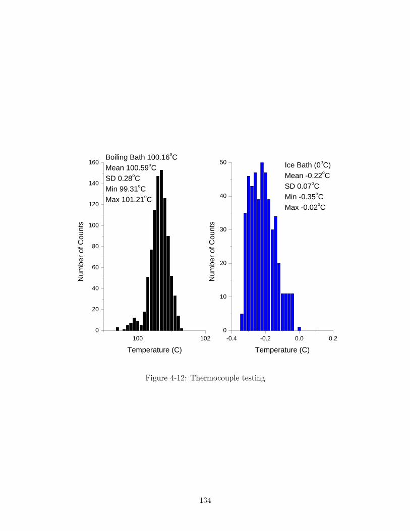
100 1020
20
40
60
80
100
120
140
160Boiling Bath 100.16oCMean 100.59oCSD 0.28oCMin 99.31oCMax 101.21oC
Num
ber o
f Cou
nts
Temperature (C)-0.4 -0.2 0.0 0.2
0
10
20
30
40
50 Ice Bath (0oC)Mean -0.22oCSD 0.07oCMin -0.35oCMax -0.02oC
Num
ber o
f Cou
nts
Temperature (C)
Figure 4-12: Thermocouple testing
134

4.2.5 Differential Pressure Transducer
The differential pressure transducer, Omega PX293-030D5V, operates over a range
of 0− 30psid(0− 207kPa) with accuracy to within 0.5% of the reading as calibrated
by the manufacturer. The output is a linear curve scaled from 0− 5DCV for the full
scale pressure. No additional calibration is required.
4.3 Water convection testing
After completion of construction and calibration of the flow loop, testing of the loop’s
functionality for measuring heat transfer coefficient and viscous pressure loss is re-
quired. The initial test is done with water, whose performance and properties are well
known from literature. Six initial tests are run with various flow rates and inlet tem-
peratures. The test are operated for Reynolds numbers betwenn 18,000 and 65,000
with heat flux of 100kW/m2. Inlet temperatures are varied between 20oC and 60oC
to maintain the wall temperature below the boiling point. All tests are performed
at atmospheric pressure. These tests prove the apparatus for heated turbulent flows
against existing friction factor and heat transfer coefficient correlations found in the
literature. All raw data for the test is given in Appendix D.
4.3.1 Heat transfer coefficient water test
First the heat transfer coefficient is compared by means of the local Dittus-Boelter-
type correlation for Nusselt number,
Nux = 0.023Re0.8x Pr0.4
x = 0.023
(ρDv
µ
)0.8
x
(µcp
k
)0.4
x, (4.4)
where D is the tube inner diameter, v is the average velocity, ρ is the density, cp is the
specific heat capacity, and µ is the viscosity all evaluated at the local axial position.
The following steps are used in the calculation of the heat transfer coefficient:
135

Power
Power is measured directly from the test section current, I, and voltage difference,
V , assuming no heat losses Q = IV and heat flux on the tube inner wall as
q” =Q
πDinL
. The heat loss assumption is proven through the energy balance and the bulk tem-
perature rise in the next step.
Bulk and Wall Temperature
The flow rate is measured from the volumetric flow rate, AV , and the bulk inlet
temperature, Tb,in, for the density, ρ, as m = ρAV . Local bulk temperature is in-
terpolated using the conservation of energy as Tb(x) = Q/mcp + Tb,in. This value is
compared with the bulk outlet temperature which is also measured to assure mini-
mization of heat loss. All the experiments determined that this error is usually less
than 1% for the heat fluxes under investigation and therefore it is assumed that heat
losses will not alter the results substantially.
Wall temperature is measured on the outer surface, Tw,o, of the tube and the inner
wall temperature, Tw,i, is found through the analytical solution for the conduction
through the tube as
Tw,i = Tw,o −Q
2πkwL
[D2
o
(D2o −D2
i )log
(Do
Di
− 1/2)]
where the temperature dependent thermal conductivity of stainless steel is found
from a linear curve fit of data found in the ASM Handbook [71], as shown in Figure 4-
13. The resulting linear fit for the temperature dependent is the following funtion
kw(T ) = 0.0127 ∗ T + 13.23188.
136

0 50 100 150 200
13.5
14.0
14.5
15.0
15.5
16.0
Y = A + B * XParameter Value Error------------------------------------------------------------A 13.23188 0.07786B 0.0127 6.02579E-4------------------------------------------------------------R SD N P------------------------------------------------------------0.99888 0.07995 3 0.03018------------------------------------------------------------
Ther
mal
Con
duct
ivity
(W/m
2 -o C)
Temperature (oC)
ASM Handbook Linear Fit of Data
Figure 4-13: Temperature dependence of stainless steel 316 thermal conductivity
137

0 20 40 60 80 100 120 140 160 180 200 220 240 260 280 3000
20
40
60
80
100
120
140
160
180
200
220
240
260
280
300
Data Points +/-10% +/-20%
Mea
sure
d N
usse
lt N
umbe
r
Predicted Nusselt Number
Figure 4-14: Water test Nusselt number comparison to theory
Heat transfer coefficient
The local heat transfer coefficient is defined as
hx =q”
(Tw,i − Tb)x
where all of the terms are defined above. This can be compared with the value
predicted by equation where hx = Nuxkb,x/Di with kb,x as the bulk liquid thermal
conductivity. It can be seen in Figure 4-14 that most of the data land within 10%
of the predicted values and all of the data including the uncertainty land within 20%
of the prediction. Uncertainty analysis can be found in Appendix C. A sample wall
temperature profile is provided for one of the cases in Figure 4-15. Each case records
around 40 points in time over around 100 seconds. This assures that the system
138

0.0 0.5 1.0 1.5 2.0 2.5 3.0
22
24
26
28
30
32
34
36
38
40
42
44
46
Tem
pera
ture
(o C)
Axial Location (m)
Linear Fit (SD = 0.46oC) Wall Bulk
Figure 4-15: Test wall temperature profile
has achieved steady state. It can be seen that the time dependence (error bars) are
insignificant. However, it is noticed that there is a small axial temperature variation
on the wall. It is assumed this is due to contact resistance and normal thermocouple
offsets. If one makes a line fit it can be seen that the values standard deviation is less
than the specified value of 0.5oC. For this reason and for ease of comprehension of
data, the tube average heat transfer coefficient and Nusselt number will be used, as
shown in Figures 4-16 and 4-17. It is found that this reduces clutter and shows the
desired results in an easier to comprehend fashion, without loss of information.
139

20000 30000 40000 50000 60000 70000
2000
3000
4000
5000
6000
7000
8000
9000
10000
11000
12000
h/P
r0.4 (W
/m2 K
)
Reynolds Number
Data Points 0.023*Re0.8
Figure 4-16: Normalized heat transfer coefficient
140

0 50 100 150 200 250 3000
50
100
150
200
250
300
Data Points +/-10%
Mea
sure
d N
usse
lt N
umbe
r
Predicted Nusselt Number
Figure 4-17: Water test tube-average Nusselt number comparison to theory
141

4.3.2 Viscous pressure loss water test
The heated and isothermal sections are used to provide viscous pressure loss data for
the six cases investigated above. Values measured can be compared to the correlated
theory where pressure loss is
∆P = ffL
D
ρv2
2(4.5)
where L and D are the length and diameter of the tube and the friction factor ff can
be determined in the fully developed turbulent flow regime from
ff = 0.316Re−0.25, (4.6)
the Blasius relation, if Re < 30000 or else
ff = 0.184Re−0.2, (4.7)
the McAdams relation. The test section is horizontal and has a constant flow area,
thus gravitational, acceleration and form pressure terms can be neglected in Eq.
4.5. Also, a calming section at the entrance of the test section ensures that fully-
developed flow is achieved before the pressure drop is measured. The results can
be seen in Figure 4-18. The measured values land to within 10% of the predicted
values. If one considers the friction factors, the results can be seen in Figure 4-19.
The friction factors and the uncertainty land well within 20% of the predicted values.
Uncertainty analysis is presented in Appendix C. From these results, it is presumed
that the experiment is functioning properly. Completion of the water testing proved
the apparatus is capable of measuring heat transfer coefficient and viscous pressure
drop for liquids effectively. The testing also allowed for the development of operation
practices, software, and data reduction methodology. The data reduction software
developed in MATLAB is presented in Appendix D.
142

0 5000 10000 15000 20000 25000 300000
5000
10000
15000
20000
25000
30000
Heated Isothermal
+/-10%
Mea
sure
d P
ress
ure
Loss
(Pa)
Predicted Pressure Loss (Pa)
Figure 4-18: Water test viscous pressure loss comparison
143

10000 20000 30000 40000 50000 60000 70000
0.016
0.018
0.020
0.022
0.024
0.026
0.028
0.030
0.032
0.034
0.036Blausius McAdams
Fric
tion
Fact
or
Reynolds Number
Heated Isothermal Correlation +/-20%
Figure 4-19: Test friction factor comparison
144

4.4 Nanofluid Convection Experiments
This section covers the most important piece of this work, which is the nanofluid
convective heat transfer and viscous pressure loss experiments. The methodology is
discussed below and the experiments follow. First, the alumina nanofluid from Nyacol
will be tested. After this run, the loop will be cleaned using water and then tested
with water to assure no deposition will alter the outcome. Finally, the zirconia will
be tested. These results are interpreted through some theoretical analysis. All raw
data for the test is given in Appendix D.
4.4.1 Methodology
The implementation of nanofluids in the loop requires some additional actions. It
is desired to run the loop with different nanoparticle loadings and with different
nanoparticles (Al2O3 and ZrO2). It is key to know the loadings in order to utilize the
correct properties in the evaluation of the data. For this reason the loop will be loaded
with the maximum desired loading and then diluted to lower loadings. In order to
get the desired loadings, an approximate loop volume is required. The loop volume is
estimated to be roughly 7 liters. Therefore, the loop will be loaded at the maximum
and then 3.5 liters will be removed and replaced with water between experimental
runs. Three loadings are measured for each nanofluid. The removed nanofluids are
kept for verification of the nanofluid properties, most especially the loading.
Each nanofluid is investigated at various flow rates, bulk inlet temperatures, and
heat fluxes. The heat flux should have only limited effect on the nanofluid (via change
in the wall viscosity) if it is behaving like a normal fluid. Bulk inlet temperature
variation should catch if there is any temperature enhancing effect on the nanofluid.
The flow rates should determine if there is any turbulent mixing effect of the nanofluid.
4.4.2 Alumina Results
The Nyacol alumina is run for three different loadings as follows: 0.9 vol% (3.53 wt%),
1.8 vol% (7.06 wt%), and 3.6 vol% (14.11 wt%). The weight loadings were verified
145

0 50 100 150 200 250 3000
50
100
150
200
250
300
-10%
+10%
Mea
sure
d N
usse
lt N
umbe
r
Predicted Nusselt Number
Al (0.9 vol%) Al (1.8 vol%) Al (3.6 vol%)
Figure 4-20: Nyacol alumina tube-average Nusselt number comparison to theory
after the experiment using TGA. The conversion between weight and volume fraction
is done through the assumed density of 3920 kg/m3 for the alumina.
Nyacol Alumina Nusselt Number
The measured Nusselt number is compared to that of the predicted Nusselt number of
the Dittus-Boelter equation, as defined in Equation 4.3.1, which predicts most fluids
to within ±20% of experiment. Properties of the nanofluid are determined from the
temperature and loading dependent properties as defined in Section 3.9. The resulting
plot is shown in Figure 4-20. It can be seen in the figure that the Nusselt number is
effectively predicted by the Dittus-Boelter equation to within ±10%, if the properties
of the nanofluid are used.
146

0 5000 10000 15000 20000 25000 30000 35000 400000
5000
10000
15000
20000
25000
30000
35000
40000
-20%
+20%
Mea
sure
d V
isco
us P
ress
ure
Loss
(Pa)
Predicted Viscous Pressure Loss (Pa)
Heated Isothermal 0.9 v% 0.9 v% 1.8 v% 1.8 v% 3.6 v% 3.6 v%
Figure 4-21: Nyacol alumina viscous pressure loss comparison
Nyacol Alumina Viscous Pressure Losses
The viscous pressure loss is also compared to the theoretical loss predicted by Blasius
and McAdams correlations, Equations 4.6 and 4.7, which predict most fluids to within
±20% of experiment. The heated and isothermal pressure drop sections are both
investigated and compared to theory. The viscous pressure losses are compared in
Figure 4-21 and the friction factors in Figure 4-22. It can be seen in the figures that
the viscous pressure losses and friction factors are effectively predicted by the theory
within ±20%, if the properties of the nanofluid are used.
147

0 10000 20000 30000 40000 50000 60000 700000.0140.0160.0180.0200.0220.0240.0260.0280.0300.0320.0340.0360.0380.0400.0420.0440.046
Fric
tion
Fact
or
Reynolds Number
Theory +/- 20% Heated Isothermal
0.9 v% 0.9 v% 1.8 v% 1.8 v% 3.6 v% 3.6 v%
Figure 4-22: Nyacol alumina friction factor comparison
148

0 20 40 60 80 100 120 140 160 180 200 220 240 260 2800
20
40
60
80
100
120
140
160
180
200
220
240
260
280
-10%
+10%
Mea
sure
d N
usse
lt N
umbe
r
Predicted Nusselt Number
Figure 4-23: Water retest tube-average Nusselt number comparison to theory
4.4.3 Water Retest Results
After completion of the alumina testing, the loop is drained completely and flushed
several times to remove the remaining nanoparticles. However in order to insure there
are no surface modifications or fouling in the system, water is once again run and
compared to theory. The tube average Nusselt number is shown in Figure 4-23 and the
viscous pressure losses are shown in Figure 4-24 It is found that the results are similar
to those of the initial tests. It is therefore concluded that no major modification of
the tube surface occurred due to the usage of nanofluids.
149

0 5000 10000 15000 20000 25000 30000 35000 40000 45000 500000
5000
10000
15000
20000
25000
30000
35000
40000
45000
50000
-10%
+10%
Mea
sure
d V
isco
us P
ress
ure
Loss
(Pa)
Predicted Viscous Pressure Loss (Pa)
Heated Isothermal
Figure 4-24: Water retest viscous pressure loss comparison
150

4.4.4 Zirconia Results
The Nyacol zirconia is run for three different loadings as follows: 0.2 vol% (1.1 wt%),
0.5 vol% (2.75 wt%), and 0.9 vol% (4.95 wt%). The weight loadings were verified
after the experiment using TGA. The conversion between weight and volume fraction
is done through the assumed density of 5500 kg/m3 for the zirconia.
Nyacol Zirconia Nusselt Number
As earlier, measured Nusselt number is compared to that of the predicted Nusselt
number of the Dittus-Boelter equation, as defined in Equation 4.3.1, which predicts
most fluids to within ±20% of experiment. The temperature and loading dependent
properties in Section 3.9 are used to calculate the non-dimensional groups. The
resulting plot is shown in Figure 4-25. It can be seen in the figure that the Nusselt
number is effectively predicted by the Dittus-Boelter equation to within ±10%, if the
properties of the nanofluid are used.
Nyacol Zirconia Viscous Pressure Losses
The viscous pressure loss is also compared to the theoretical loss predicted by Blasius
and McAdams correlations, Equations 4.6 and 4.7, which predict most fluids to within
±20% of experiment. The heated and isothermal pressure drop sections are both
investigated and compared to theory. The viscous pressure losses are compared in
Figure 4-26 and the friction factors in Figure 4-27. It can be seen in the figures that
the viscous pressure losses and friction factors are effectively predicted by the theory
within ±20%, if the properties of the nanofluid are used.
151

0 50 100 150 200 250 3000
50
100
150
200
250
300
-10%
+10%
Mea
sure
d N
usse
lt N
umbe
r
Predicted Nusselt Number
Zr (0.2 vol%) Zr (0.5 vol%) Zr (0.9 vol%)
Figure 4-25: Nyacol zirconia tube-average Nusselt number comparison to theory
152

0 5000 10000 15000 20000 25000 30000 35000 400000
5000
10000
15000
20000
25000
30000
35000
40000
-20%
+20%
Mea
sure
d V
isco
us P
ress
ure
Loss
(Pa)
Predicted Viscous Pressure Loss (Pa)
Heated Isothermal 0.2 v% 0.2 v% 0.5 v% 0.5 v% 0.9 v% 0.9 v%
Figure 4-26: Nyacol zirconia viscous pressure loss comparison
153

0 10000 20000 30000 40000 50000 60000 700000.0140.0160.0180.0200.0220.0240.0260.0280.0300.0320.0340.0360.0380.0400.0420.0440.046
Fric
tion
Fact
or
Reynolds Number
Theory +/- 20% Heated Isothermal
0.2 v% 0.2 v% 0.5 v% 0.5 v% 0.9 v% 0.9 v%
Figure 4-27: Nyacol zirconia friction factor comparison
154

Figure 4-28: DLS of Nyacol alumina 3.6 vol%
4.5 Post Test Nanofluid Characterization
It is important to recheck the particle diameters using DLS after the experiment
is completed to reassure the nanometer scales have been retained. It can be seen in
Figures 4-28, 4-29, 4-30, 4-31, 4-32, and 4-33 that the particle size remained relatively
the same as the initial size in the fully loaded colloid. Therefore it is determined that
no major agglomeration occurred during the testing.
4.6 Data Interpretation
In their experiments with and analyses of nanofluids, Pak and Cho [34], Xuan and
Roetzel [35] and Xuan and Li [2] assumed that convective heat transfer enhancement
could come from dispersion of the suspended nanoparticles. However, a mechanistic
description of particle dispersion in nanofluids has shown that this effect is very small
by Buongiorno [43].
155

Figure 4-29: DLS of Nyacol alumina 1.8 vol%
Figure 4-30: DLS of Nyacol alumina 0.9 vol%
156

Figure 4-31: DLS of Nyacol zirconia 0.9 vol%
Figure 4-32: DLS of Nyacol zirconia 0.5 vol%
157

Figure 4-33: DLS of Nyacol zirconia 0.2 vol%
Xuan and Li [2] also proposed that the enhancement could come from intensifi-
cation of turbulence due to the presence of the nanoparticles. However, our pressure
drop measurements as well as measurements by Xuan and Li [2] and Pak and Cho [34]
clearly show that turbulent friction factors in nanofluids can be very well predicted
by the traditional friction factor correlations for pure fluids, if the measured nanofluid
viscosity is used. This suggests that, beyond the obvious viscosity effect, turbulence
is not affected by the presence of the nanoparticles. This conclusion is corroborated
by a comparison of the time and length scales for the nanoparticles and the turbulent
eddies, as explained next.
A comparison of the time scale of the heat transfer from the particle to the gas
with the time scale of the particle slip motion in the water can be used to determine
the thermal equilibrium characteristics of the mixture. The heat transfer time scale
is mainly dependent on the particle to fluid conduction (τcon). The values for τcon
are found to be on the order of 10−9 to 10−7 seconds in gases, see Figure F-3. These
158

values are expected to be even smaller in a liquid due to the higher density of the
surrounding liquid. In turbulent flow the dominant slip mechanism is from inertial
flight following the abrupt stop of an eddy. The time scale for this process is the
so-called relaxation time of the particle
τrel =ρpd
2p
18µ(4.8)
Evaluation finds that τcon τrel , it is concluded that particles can exchange energy
very effectively as they fly within the liquid; therefore we can assume that there is
local particle/liquid thermal equilibrium.
Heat transfer enhancement due to turbulence strengthening is quantified analyt-
ically to justify why the results of our experiments above are logical. Due to their
small size, nanoparticles can be entrained in both large and small turbulent eddies.
This is shown by the size (l), velocity (V ) and time scales (τ) of the eddies as follows:
Scales for large eddies:
• lo ∼ 0.07 ·D = 0.07 · 9.4mm = 0.658mm
• Vo ∼ Vshear ∼ 0.9− 3.6m/s where Vshear = τw
µ
• τo ∼ lo/Vo ∼ 1.9− 7.3 · 10−4sec
Scales for small eddies (using Kolomogorov’s scaling laws [72]):
• ls/lo ∼ Re−3/4 ⇒ ls ∼ 0.17− 0.69µm
• τs/τo ∼ Re−1/2 ⇒ τs ∼ 0.8− 7.5 · 10−6sec, Vs ∼ ls/τs ∼ 0.09− 0.22m/s
It is seen that the particles (40-75nm) are smaller than the eddy sizes (0.658mm and
0.17-0.69µm). Therefore, turbulent eddies can in principle carry nanoparticles.
The next step is to determine the stopping distance (S) for the particles entrained
in the small and large eddies in order to see how far they can be thrown by the eddy
velocities. It is found that [73]
So =ρpd
2p
18µVo ∼ 0.4− 1.5µm (4.9)
159

for particles entrained by large eddies and
Ss =ρpd
2p
18µVs ∼ 40− 99nm (4.10)
for particles entrained by small eddies. This suggests that nanoparticles do not sig-
nificantly project out of the eddies with the possible exception of those entrained
by small eddies. That is, the nanoparticles move with the turbulent eddies. Thus,
contribution of inertial slip to nanoparticle dispersion is probably negligible. Regard-
ing the question of turbulence intensification, the presence of the nanoparticles does
increase viscosity, which will delay the onset of turbulence for given mean velocity.
Moreover, the stopping distance suggests that particles entrained by large eddies
may interact with (i.e., break up) small eddies, since their length scales are compa-
rable. Based on order-of-magnitude estimates of the kinetic energy carried by each
eddy and using Kolomogorov’s scaling laws, one finds that the ratio of the number of
small eddies generated per unit time and volume to the number of large eddies gener-
ated per unit time and volume is proportional to Re11/4, which in our case is greater
than 1010. Therefore, small eddies are much more numerous than large eddies. This
means that nanoparticles being projected out of large eddies will affect only a very
limited number of small eddies due to their vast numbers. In summary, an effect of
the nanoparticles on turbulence beyond the obvious effect via the change in viscosity
seems unlikely.
Finally, a major logic flaw will be discussed involving the previous works on turbu-
lent convective heat transfer in nanofluids. The other major works [2], [34] pronounce
enhancement of the convective heat transfer coefficients for nanofluids in tubes. The
major issue is the plotting of heat transfer coefficient as a function of dimensionless
Reynolds number. The nanofluids do have a higher heat transfer coefficient when
compared at the same Reynolds number as a water flow. This is due to the increase
in the Prandtl number. If one replots the existing data in the literature with heat
transfer coefficient normalized by Pr0.4 evaluated with the nanofluid properties, then
it is obvious that this is the cause of the higher heat transfer coefficients as reported
160

in the literature.
The increase of Prandtl number comes from an increase in viscosity. What is not
reported by the previous works is the large penalty in pumping power incurred by
this increased viscosity. If one analyzes the data from a prospective of the ratio of
increased heat transfer to the increase of the pumping power, it is found that the
nanofluids are not an enhancement over the use of the pure water base fluid.
4.7 Conclusions
It is concluded that the nanofluids behave in a similar fashion to single-phase fluids,
if one considers the temperature and concentration dependent nanofluid properties.
It is therefore proven that the existing empirical correlations for viscous pressure
drop and convective heat transfer coefficient in a tube describe the behavior of the
nanofluids investigated. Nanoparticles in the fluids do remain at their original size,
even through dilution. It is also shown theoretically how the nanoparticles would not
be expected to modify the large turbulent eddies nor large numbers of small eddies and
hence modify the structure of turbulence. This is confirmed by the experiments where
friction factors behave under the same Reynolds dependence as typical single-phase
fluids. Therefore nanofluid efficacy can be considered through properties evaluation
alone.
161

162
Chapter 5
Efficacy of Nanofluids as Coolants
It has been seen that the nanofluids under investigation behave as single-phase liquids
in turbulent flow and convective heat transfer in a heated tube. This creates the ability
to directly compare nanofluid performance with the performance of other coolants, in
particular water, through consideration of the fluid properties. Comparison of coolant
performance has been studied previously for nuclear reactor and other applications.
It usually involves investigation of the pumping power required to achieve certain heat
removal goals under certain constraints, for example, a limited maximum temperature
in the system. The methodology to be described and utilized here is that of Bonilla
from the Nuclear Engineering Handbook [74]. However, this methodology can be
applied also to non-nuclear systems where convective heating or cooling is involved,
such as, electronic devices, chemical reactors, engines, etc. It will be shown that
nanofluids can be optimized and that under certain conditions will outperform water.
5.1 Comparison of Coolants
Various factors can be considered for the selection of coolants, i.e. economics, hazards,
neutronic effects, etc. An initial rough comparison can be done through consideration
of the thermophysical properties of the coolant. This is most directly seen as a
ratio of the required pumping power for two coolants under certain constraints. The
most relevant constraints to consider for practical applications are a fixed is coolant
163

temperature rise (∆tc) and a fixed coolant-film temperature difference (∆tf ).
5.1.1 Pumping power
The pumping power or work required to circulate a coolant can be calculated as
Ppump = ∆Pm
ρ(5.1)
where ∆P is the pressure drop, m is the mass flow rate and ρ is the coolant density.
The viscous pressure loss is
∆Pf =ffm
2L
2DρS2(5.2)
where D is the effective diameter of the flow geometry, S is the cross sectional area
of the flow, and ff is the friction factor and can be calculated from Eq. 4.7. If
Eqs. 5.1, 5.2, and 4.7 are combined one can find the pumping power for an incom-
pressible fluid is
Ppump =0.092L
D1.2S1.8
[µ0.2
ρ2
]m2.8 (5.3)
where L is the effective length of the flow channel. In the case of laminar flow the
equation can be modified with the friction factor defined as ff = C/Re where for
round tubes C = 64 thus making
Ppump =128L
D2S
[µ
ρ2
]m2 (5.4)
It can be seen that under the same constraints the coolant performance can be com-
pared through the properties groups contained in the brackets of Eqs. 5.3 and 5.4. A
ratio of these groups for two different coolants is a rough direct comparison of their
performance. However further constraints must be supplied to make the comparison
more definitive.
164

5.1.2 Constant coolant temperature rise
First consider a system that has a large bulk temperature difference from inlet to
outlet as compared to the film temperature difference (∆tc >> ∆tf ), which would be
the case for small diameter, long channels with low heat flux. If the bulk temperature
difference is held to be constant. The substitution of q/cp∆tc for m in Eqs. 5.3 and 5.4
gives
Ppump =0.092Lq2.8
D1.2S1.8∆t2.8c
[µ0.2
ρ2c2.8p
](5.5)
for turbulent flow and
Ppump =128L
D2S
q2
∆t2c
[µ
ρ2c2p
](5.6)
for the case of laminar flow. The groups contained in the brackets contain the effects
due to the coolant properties. It can be seen that viscosity, density, and heat capacity
are the only important properties and thermal conductivity is of no importance under
the sole constraint of fixed ∆tc.
5.1.3 Constant coolant-film temperature difference
Now consider a system that has a large film temperature difference as compared to the
bulk temperature difference from inlet to outlet (∆tf >> ∆tc), which would be the
case for larger diameter, short channels with high heat flux. If the film temperature
difference is held constant (i.e. heat transfer coefficient is held constant). Utilizing
the Dittus-Boelter correlation Nu = hD/k = 0.023Re0.8Pr0.4 to find the average
velocity (or mass flow rate) it is found that
Ppump =49850LSh3.5
D0.5
[µ1.835
ρ2c1.167p k2.4
](5.7)
for fully developed turbulent flow in a tube of non-metallic coolants and
Ppump = 5.66L3D2h6
[µ
ρ2c2pk
4
](5.8)
for the case of laminar flow.
165

In the light of analysis and derivation presented in the previouspaper @10#, the following formula is proposed to correlate theexperimental data for the nanofluid:
Nun f5c1~1.01c2fm1Pedm2!Ren f
m3Prn f0.4 (6)
Compared with the heat transfer correlation for conventionalsingle-phase flow, the volume fractionf of suspended nanopar-ticles and the Peclet number are involved in the above expression.The Peclet number Pe describes the effect of thermal dispersioncaused by microconvective and microdiffusion of the suspendednanoparticles. The casec250 refers to zero thermal dispersion,which namely corresponds to the case of the pure base fluid. Theparticle Peclet number Ped in expression~6! is defined as
Ped5umdp
an f(7)
The Reynolds number of the nanofluid is defined as
Ren f5umD
yn f(8)
The Prandlt number Pr of the nanofluid is defined as
Prn f5yn f
an f(9)
To calculate this parameter, the thermal diffusivity of the nanof-luid an f is defined as
an f5kn f
~rcp!n f5
kn f
~12f!~rcp! f1f~rcp!d(10)
Where, the thermal conductivitykn f and the viscosityyn f are ex-perimentally obtained and the experimental procedure is describedin detail in reference@6#. Some experimental data are listed inTable 1.
From the whole ensemble of experimental data, the coefficientc1 andc2 as well as the exponentm1 , m2 , andm3 in expression~6! can be determined by a proper data-reduction procedure. For agiven flow velocity, a set of all these coefficients and exponents isfit for predicting heat transfer performance of nanofluids with dif-ferent volume fractions of suspended nanoparticles. For a varietyof volume fraction of suspended nanoparticles, for example, theNusselt number Nu for the turbulent flow of nanofluids inside atube are obtained as follows:
Nun f50.0059~1.017.6286f0.6886Ped0.001!Ren f
0.9238Prn f0.4 (11)
Figure 5 depicts the curves of the theoretical predictions ofconvective heat transfer coefficients of nanofluids from correla-tion ~11!. Obviously, there exists good coincidence between theresults calculated from this correlation and the experimental ones.The discrepancy between both them falls below 8 percent. It re-veals that formula~6! correctly incorporates the main factors ofaffecting heat transfer process of the nanofluid into in a simplerform and can be used to correlate experimental data of heat trans-fer coefficient of the nanofluid. Once all the coefficients and ex-ponents in formula~6! have been determined by correlating ex-perimental data of heat transfer for nanofluids, therefore, this
formula can be used to predict the convective heat transfer coef-ficient for such suspensions with different volume fractions ofnanoparticles in the turbulent flow.
4 Pressure Drop ExperimentIt is necessary to learn the flow resistance of nanofluids besides
the heat transfer enhancement feature in order to apply the nanof-luid to practical cases. The pressure drops of the dilute suspen-sions consisting of water and Cu-nanoparticles in a tube are ex-perimentally measured for the turbulent flow.
Four sample nanofluids with the volume fractions of nanopar-ticles 1.0 percent, 1.2 percent, 1.5 percent, and 2.0 percent areused in pressure drop test. Figure 6 illustrates the friction factorsas a function of the Reynolds number for the turbulent flow. Thefriction factor of the pure water is also shown as a solid line in thefigures. The friction factor is defined as
ln f5Pn fD
L
2g
um2 (12)
Obviously, the friction factors of the dilute nanofluids are al-most equal to those of water under the same Reynolds number.Compared with water, no significant augmentation in pressuredrop for the nanofluid is found in all runs of the experiment,
Table 1 The effective thermal conductivity and viscosity of thesample nanofluid
Transportproperties
Volume fraction of nanoparticles
0.3% 0.5% 0.8% 1.0% 1.2% 1.5% 2.0%
kn f ~W/m•°C! 0.6054 0.615 0.6252 0.6306 0.633 0.663 0.702yn f3106 (m2/s) 0.91 0.915 0.945 0.96 1.012 1.044 1.125
Fig. 5 Comparison between the measured data and the calcu-lated values from correlation „11… for turbulent flow
Fig. 6 The friction factors of nanofluids for the turbulent flow
154 Õ Vol. 125, FEBRUARY 2003 Transactions of the ASME
Figure 5-1: Properties of copper water nanofluids from Xuan and Li [2]
5.2 Efficacy of Nanofluids
Using the above described methodologies we will define the efficacy of a coolant as
the ratio of the property parameters in brackets with that of water. For example, for
the constant coolant temperature rise in turbulent flow case as given in Equation 5.5
the efficacy would be defined as
[µ0.2
ρ2c2.8p
]water[
µ0.2
ρ2c2.8p
]coolant
(5.9)
Therefore if the coolant has better performance than that of water (which is nominally
the best selection) then the efficacy would be greater than unity. Properties of zirco-
nia and alumina nanofluids are calculated using the models proposed in Section 3.9.
The properties for copper in water are determined from curve fits of the properties
given by Xuan and Li [2], which was only to a volume fraction of 2%, see Figure 5-1.
The efficacy for each fluid under the above constraints is calculated and plotted in
Figures 5-2, 5-3, 5-4, and 5-5. It can be seen that the only potentially beneficial
nanofluid is the copper under the laminar constant film temperature case. The major
issue is that the dominating factor is typically the viscosity and not the conductivity.
The product of density and heat capacity remains relatively constant for all materi-
als, except for porous insulators. However there is also a mild dependence on heat
capacity, C0.8p , which is typically lower for the water nanofluid than the base water.
The other main issue is the large increase in viscosity associated with the nanoparticle
166

0.00 0.01 0.02 0.03 0.04 0.050.0
0.2
0.4
0.6
0.8
1.0E
ffica
cy
Volume Fraction
Al Zr Cu
Figure 5-2: Efficacy of nanofluids under laminar bulk temperature rise constraint
dispersions. Likewise in order to increase the stabilization requires increasing surface
charge density, which in turn increases the viscosity. The thermal conductivity effect
may become important in the constant film temperature cases, primarily for laminar
flow and only in the case for nanofluids with high thermal conductivity enhancement
such as Cu based nanofluids..
5.3 Conclusions
Assuming that nanofluids behave in the same fashion as single-phase fluids, it was
shown that the efficacy for these fluids can be determined theoretically if the prop-
erties are known. It is determined that the nanofluids tested in this study afford no
enhancement for turbulent convective heat transfer enhancement at a given pump-
167

0.00 0.01 0.02 0.03 0.04 0.050.0
0.2
0.4
0.6
0.8
1.0
Effi
cacy
Volume Fraction
Al Zr Cu
Figure 5-3: Efficacy of nanofluids under turbulent bulk temperature rise constraint
168
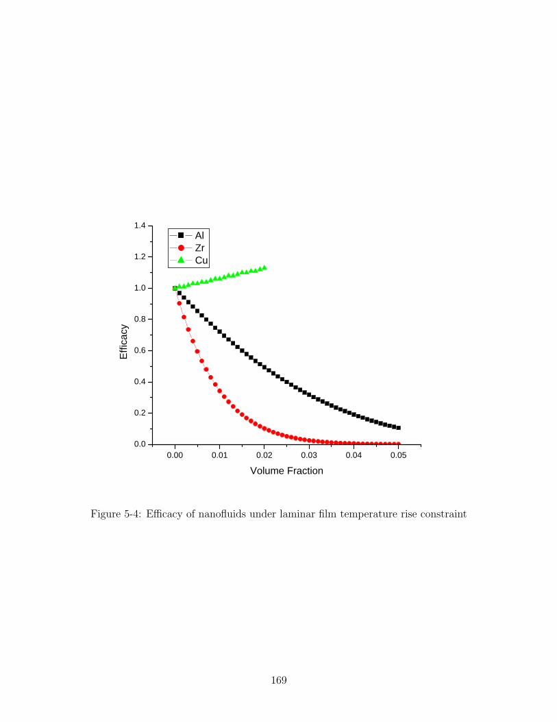
0.00 0.01 0.02 0.03 0.04 0.050.0
0.2
0.4
0.6
0.8
1.0
1.2
1.4
Effi
cacy
Volume Fraction
Al Zr Cu
Figure 5-4: Efficacy of nanofluids under laminar film temperature rise constraint
169

0.00 0.01 0.02 0.03 0.04 0.050.0
0.1
0.2
0.3
0.4
0.5
0.6
0.7
0.8
0.9
1.0
1.1
Effi
cacy
Volume Fraction
Al Zr Cu
Figure 5-5: Efficacy of nanofluids under turbulent film temperature rise constraint
170

ing power. However fluids could possibly be beneficial to short channel high heat
flux laminar flow situations. It is very important to maintain the viscosity as low as
possible, while obtaining the thermal conductivity enhancement, which is intuitive.
Our experiments suggest that nanofluids convective heat transfer can be accurately
described using traditional homogenous-medium theories. However such theories do
not account for potential enhancement of heat transfer in the developing length, which
has been shown to be important in laminar flows in recent works on nanofluids, like
Ding et al. [75].
Another problem is the usage of nanoparticles in the enhancement of the thermal
properties of other coolants like ethylene glycol or refrigerants. It is important to
remember that these coolants are used for particular purposes besides their heat
transfer capability. Water is a superior heat transfer medium typically, however other
coolants are better under certain temperature constraints. Ethylene glycol is typically
used when the operating temperature is expected to drop below the freezing point of
water. Likewise refrigerants are used for their higher volatility or ability to evaporate.
It is yet to be seen how the addition of particles would affect evaporation and freezing.
Studies in this area are ongoing at MIT.
171

172
Chapter 6
Conclusions
In conclusion, there are many variables that must be accounted for when dealing
with nanofluid (colloid) experiments. The conceptual and theoretical developments
of colloid and surface science lead to a far better understanding of nanofluid prop-
erties and behavior. Some properties such as size and stability are easily altered by
concentration, pH, and temperature modifications. Nanofluids are colloids and
should be investigated as such.
A description of the techniques to characterize nanofluids quantitatively has been
given. Of these techniques, DLS and TEM have been selected for particle and ag-
glomeration sizing of the nanofluids. It is determined that DLS should be the primary
method of particle sizing, due to its ease of use and low cost. However, TEM imaging
must be used in order to certify the results because of the potential for error due to
non-spherical particles and polydispersity in the system. DLS and TEM are the
best techniques to characterize particle sizes.
ICP and TGA are the best techniques for the determination of nanofluid
concentration. ICP is very effective in determining the exact elemental constituents
of the system. It can be used to find contamination down to the ppb level of multiple
elements with great ease. The major drawback of ICP is that it only determines
elemental makeup of the system and not the molecular/chemical makeup. Therefore
some calculation must be done in order to determine weight loading of nanoparticles.
For this reason TGA is a quick and easy method of determining particulate loading of
173

a system. The “cooking off” of constituents allows one to see surfactant weight load-
ing, as well as, the particle loading. Therefore a combination of the two techniques
is recommended for nanofluid characterization.
Implementation of a short hot wire thermal conductivity probe has been successful
in the determination of the thermal conductivity of basic liquids and more importantly
the nanoparticle colloids. Likewise, the glass capillary viscometer is found to be effec-
tive in the measurement of the viscosity of nanoparticle colloids at different loadings
and temperatures. It is concluded that nanofluids behave in a similar fashion
to equivalent single-phase fluids, if one considers the temperature and
concentration dependent nanofluid mixture properties.
It is proven that the traditional empirical correlations for viscous
pressure drop and convective heat transfer coefficient in a tube describe
the behavior of the nanofluids investigated. It is also shown by means of order-
of-magnitude estimates that the nanoparticles would not be expected to modify the
large turbulence eddies nor large numbers of small eddies and hence modify the flow
structure. This is reiterated by the experiments where friction factors behave under
the same Reynolds dependence as typical single-phase fluids.
Nanofluid efficacy can be considered through properties evaluation
alone. Assuming that nanofluids behave in the same fashion as single-phase flu-
ids, it is shown that the efficacy for these fluids depends only on their thermophysical
properties. It is determined that the current nanofluids are of no interest for turbulent
convective heat transfer enhancement. However fluids could possibly be beneficial to
short channel high heat flux laminar flow situations. It is very important to maintain
the viscosity as low as possible, while obtaining the thermal conductivity enhance-
ment, which is somewhat intuitive.
It is recommended that future nanofluids could be easily investigated using theory
and properties measurement. However the theory does not account for potential
enhancement of heat transfer in the developing length, which is important in laminar
flows. However, theory can be a guide for the development of future engineering
coolants like nanofluids.
174

Appendix A
Hot-Wire Numerical Studies by
Roberto Rusconi
A.1 The transient hot-wire method: numerical sim-
ulations
Numerical simulations have been performed for the THW method using a commer-
cial finite-elements solving routine, FlexPDE Professional 3D (PDE Solutions Inc.),
which requires a direct implementation of the governing equations. By exploiting the
symmetry of the problem, a 2D cylindrical model is chosen (see Figure A-1) and a
self-adapting mesh of triangular elements (derived from an analogue problem [68]).
The Navier-Stokes equations are used along with the Boussinesq approximation,
the so-called “Poisson pressure” equation, and the heat diffusion equations as:
ν∇ · ∇vr =1
ρ
∂p
∂r+ vr
∂vr
∂r+ vz
∂vr
∂z+
∂vr
∂t
ν∇ · ∇vz =1
ρ
∂p
∂r+ vr
∂vz
∂r+ vz
∂vz
∂z+
∂vz
∂t− gα∆T
∇ · ∇(p/ρ) = δ
[1
r
∂rvr
∂r+
∂vz
∂z
]+ 2
(∂vr
∂r
∂vz
∂z− ∂vr
∂z
∂vz
∂r
)− gα
∂∆T
∂z
175

Figure A-1: Computational domain used in the numerical simulations.
κ∇ · ∇(∆T ) = vr∂∆T
∂r+ vz
∂∆T
∂z+
∂∆T
∂t
where vr and vz are the radial and axial components of momentum, ρ is the density
and δ is the penalty coefficient which numerically enforces the incompressibility of
the velocity field, for more details see [68]. In contrast with [68], this case has two
different areas: the wire (solid) and the sample (liquid). As the routine doesn’t allow
the implementation of distinct equations for different regions, a parameter m which is
equal 1 in the liquid area and 0 in the solid one is used. In this way only the Fourier
equation has been solved for the wire and it was checked that this imposition didn’t
affect the solution of the other equations in the liquid part.
A.1.1 Case: simple fluid without convection
First, the results obtained by the numerical simulations for pure water (at room
temperature) in absence of natural convection (g = 0) with the theoretical analysis
are given.
176

Figure A-2: Effect of the finite boundary on the temperature rise.
177

Figure A-3: Temperature increase for different lengths of the wire.
In Figure A-2 the temperature increments (∆T is meant as an average of the
temperature field over the entire wire) are displayed for distinct ratios between the
outer radius and the radius of the wire: it is clearly seen that the logarithmic growth,
which is independent of the size of the cell but is longer for larger outer radii, and
the steady-state value, which is proportional to ln(b/a).
In Figure A-3 the results for different lengths of the wire are given: in case of
L = 25mm a value of thermal conductivity is obtained (the inverse of the slope
of the curves) equal to 0.621 Wm−1K−1, which slightly higher of the real value
0.607 Wm−1K−1. It is noticed that with shorter wires the difference from the theo-
retical model is stronger. Moreover it can seen in Figure A-4 that the temperature
rise divided by the applied power is not dependent on the input current, as expected.
178

Figure A-4: Temperature increase for different input currents.
179

Figure A-5: Numerical instabilities in the solution.
A.1.2 Case: simple fluid with convection
After verifying that the model used in the simulations is consistent with the theory
of THW, the effect of natural convection is analyzed by the same method. In order
to reduce computational times, but at the same time to preserve the accuracy of the
solution, the influence of some numerical parameters (mesh size, solution controls and
penalty factor) are investigated for their effect on the numerical results. In Figure A-5
it is noticeable that in some cases the simulations can have an oscillatory behavior,
while the full line is the accurate and mesh-independent solution.
In Figure A-6 it is seen how the temperature field after 100s is distorted by the
presence of the convective rolls in Figure A-7. In Figure A-8 the time-dependent
temperature increments with or without natural convection are compared. The pres-
ence of a velocity field produces a sensible deviation from the logarithmic trend after
some seconds. This is much more evident if it is considered that instead of taking the
180
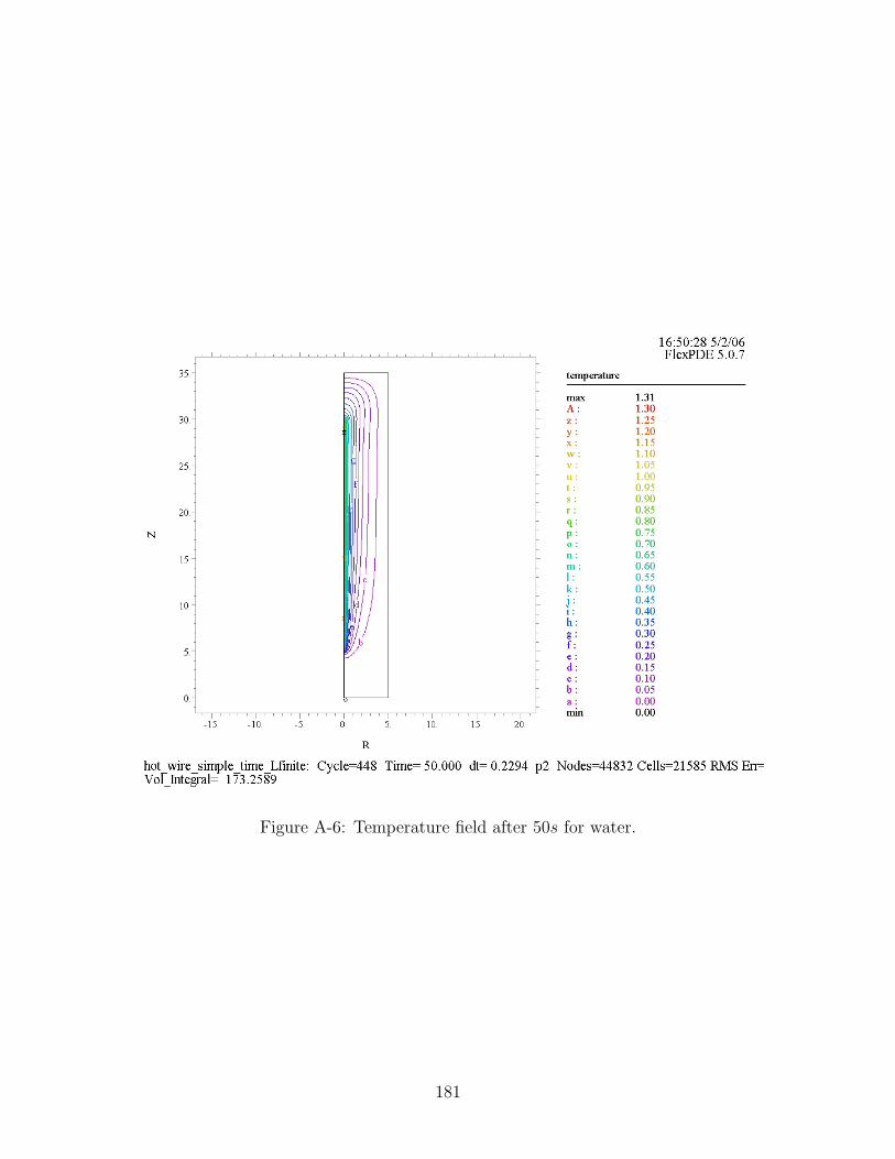
Figure A-6: Temperature field after 50s for water.
181

Figure A-7: Velocity field after 50s for water.
182

Figure A-8: Temperature increments for a wire of 25mm with and without naturalconvection.
183

Figure A-9: Comparison of the numerical results for different input currents.
average over the entire wire (L = 25mm), the temperature variations at two points
at the same distance from the top and the bottom of the wire. In the ideal case these
points, for symmetry reasons, should have always the same temperature but because
of convection the temporal evolution becomes extremely different after few seconds
and this is the same asymmetry as shown in Figure A-6.
Finally in Figure A-9 and Figure A-10 it is clear how the effect of convection is
stronger at higher applied power or higher external temperature where the viscosity
of water is lower.
184

Figure A-10: Comparison of the numerical results for an external temperature of 25and 75C. Inset: the magnitude of the velocity field for the two temperatures.
185

A.2 The transient hot-wire method in colloids: nu-
merical simulations
Similar to the previous work with pure fluids, numerical simulations are performed
for the THW method using FlexPDE Professional 3D. Once again by exploiting the
symmetry of the problem, a 2D cylindrical model is chosen (see Figure A-1) and a
self-adapting mesh of triangular elements (derived from an analogue problem [68]).
The Navier-Stokes equations are used along with the Boussinesq approximation,
the so-called “Poisson pressure” equation, and the heat and mass diffusion equations
as:
ν∇ · ∇vr =1
ρ
∂p
∂r+ vr
∂vr
∂r+ vz
∂vr
∂z+
∂vr
∂t
ν∇ · ∇vz =1
ρ
∂p
∂r+ vr
∂vz
∂r+ vz
∂vz
∂z+
∂vz
∂t− gα∆T
∇ · ∇(p/ρ) = δ
[1
r
∂rvr
∂r+
∂vz
∂z
]+ 2
(∂vr
∂r
∂vz
∂z− ∂vr
∂z
∂vz
∂r
)− gα
∂∆T
∂z
κ∇ · ∇(∆T ) = vr∂∆T
∂r+ vz
∂∆T
∂z+
∂∆T
∂t
mDm · ∇(∆c) = m · (vr∂c
∂r+ vz
∂c
∂z) +
∂c
∂t−m ·DmST A(1− A)∇(∆T )
where c is the concentration and Dm is the mass diffusion coefficient, and A is a
coefficient to prevent mass diffusion through the wire region. In contrast with [68],
this case has two different areas: the wire (solid) and the sample (liquid). As the
routine doesn’t allow the implementation of distinct equations for different regions, a
parameter m which is equal 1 in the liquid area and 0 in the solid one is used. In this
way only the Fourier equation has been solved for the wire and it was checked that
this imposition didn’t affect the solution of the other equations in the liquid part.
Also the presence of thermophoresis has been considered, expressed by the Soret
186

coefficient sT. At the boundary the no-slip condition was imposed for the momentum
and ∆T = 0, except of course for the axis of rotation where a natural condition (zero
flux) has been used.
A.2.1 Case: colloidal suspension without convection
The case of a dispersions in water are analyzed with alumina (Aluminium oxide,
Nyacol) particles of a mass fraction of around 20% and an effective radius of roughly
50nm (measured with Dynamic Light Scattering). The physical properties used in
the simulations for the particles are: ρp = 3.89 g cm−3, cp = 0.88 J g−1 K−1, λp =
35 W m−1 K−1, D = 5.22 10−6 mm2 s−1, sT = −0.023 K−1. Where D is the mass
diffusion coefficient and the Soret coefficient sT has been measured with the Thermal
Lens setup [68] at the Politecnico di Milano. The properties used for the fluid are:
φm =cm ρw
cm ρw + ρp (1 − cm)= 6%,
where φm is the average volume fractions, cm is the average mass fraction, ρw is the
density of water, the measured value for the kinematic viscosity is ν = 5.6 mm2 s−1,
and the mass expansion coefficient is
β =1
ρm
dρm
dcm
=
(ρp
ρp − ρw
− cm
)−1
. These values are held constant. It is decided for the thermal conductivity to use
the Maxwell-Garnett (MG) relation
λ = λw1 + 3 φ (λp/λw − 1)
λp/λw + 2 − φ (λp/λw − 1)
with λw the thermal conductivity of water and the local volumetric fraction of the
particles
φ =c ρw
c ρw + ρp (1 − c)
where c is the local mass concentration and both are variables.
187

Figure A-11: Comparison of the numerical results for water and alumina at g = 0.
188

Figure A-12: Concentration profile after 100s at the midpoint of the wire as a functionof the radial distance.
189

Figure A-13: Comparison of the numerical results for water and alumina with con-vection.
In Figure A-11 a comparison of the results of the numerical simulations for the
alumina dispersion with pure water are shown at g = 0: the value of thermal con-
ductivity is obtained by fitting the linear part (in a log scale) of the curves, which
gives 0.728 W m−1 K−1 and then divide it by the one found for water. This value is
found to be exactly the value given by Maxwell-Garnett, which means there should
be no influence of thermophoresis on the measurements of heat transfer with the
THW method in the ideal case in absence of convection. This is confirmed by the
concentration profile around the wire, see Figure A-12, which is too small to affect
the thermal conductivity of the sample.
190

Figure A-14: Temperature field after 100s for a suspension of alumina (20%wt).
191

Figure A-15: Velocity field after 100s for a suspension of alumina (20%wt).
192

Figure A-16: Concentration field after 100s for a suspension of alumina (20%wt).
193

Figure A-17: Concentration profile after 100s, in the case of a fictitious sT =−0.2K−1, with and without convection.
194

A.2.2 Case: colloidal suspension with convection
In Figure A-13 the results of the numerical simulations for a suspension of alumina
in presence of convection are displayed, compared to those obtained for water. In
this case, because of the high value of viscosity, the effect of buoyancy is practically
negligible: this is manifested by comparing the thermal field represented in Figure
A-14 with that of pure water (Figure A-6) or the intensity of the velocity field (see
Figure A-7 and Figure A-15) which is one order of magnitude lower. Furthermore
the convective motion slightly affects the concentration profile, see Figure A-16 and
Figure A-17, which is essentially developed close to the no-slip region.
195

196
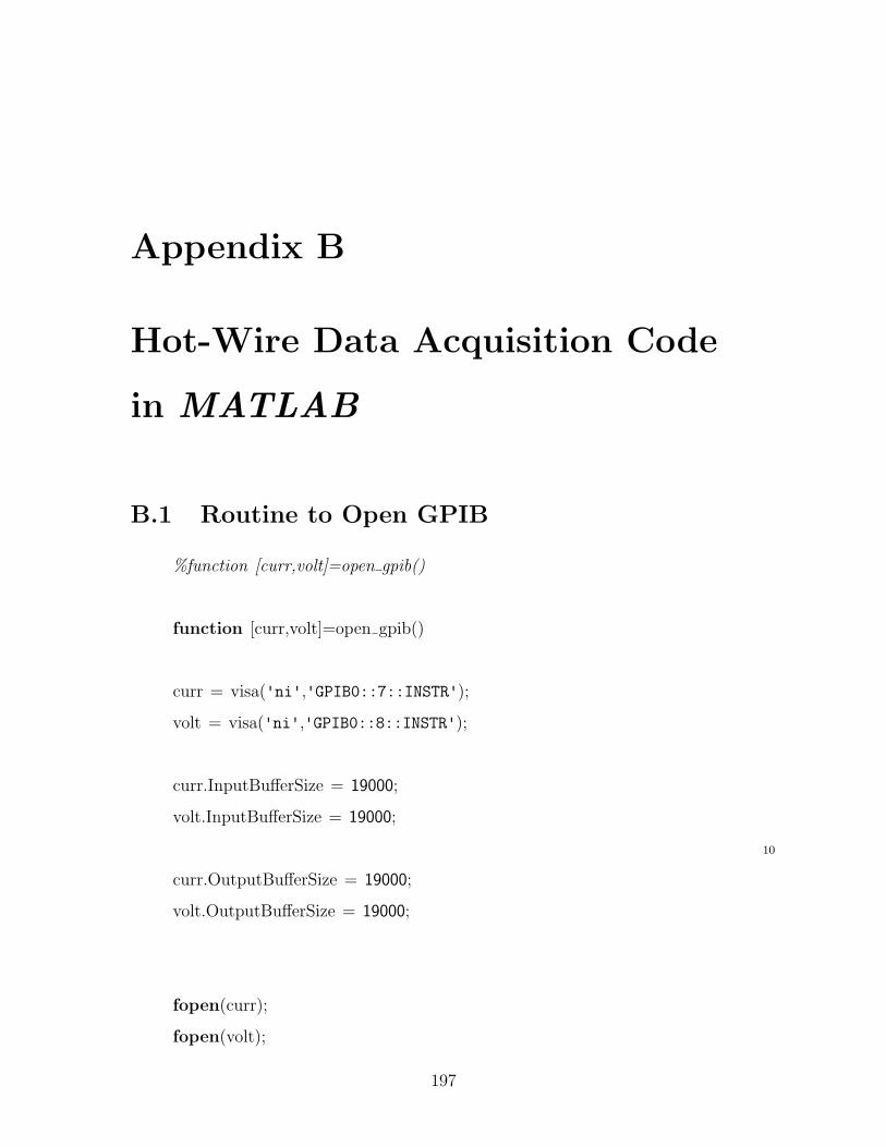
Appendix B
Hot-Wire Data Acquisition Code
in MATLAB
B.1 Routine to Open GPIB
%function [curr,volt]=open gpib()
function [curr,volt]=open gpib()
curr = visa('ni','GPIB0::7::INSTR');
volt = visa('ni','GPIB0::8::INSTR');
curr.InputBufferSize = 19000;
volt.InputBufferSize = 19000;
10
curr.OutputBufferSize = 19000;
volt.OutputBufferSize = 19000;
fopen(curr);
fopen(volt);
197

B.2 Routine to Measure Voltage Bias of Wire
function voltage=volt bias(curr,volt)
fprintf(curr,':sour:curr 0.001');
fprintf(volt,':trig:sour ext');
fprintf(volt,':trac:poin 100');
fprintf(volt,':sens:volt:nplc 0.1');
fprintf(volt,':trac:feed sens');
fprintf(volt,':trac:feed:cont next');
fprintf(volt,':trig:sour imm');
pause(1) 10
fprintf(volt,':trac:data?');
point=fscanf(volt);
pause(1)
np = size(point);
n=np(2);
i=1;
while (i<n)
if (point(i)==',')
data(i)=' '; 20
else
data(i) = point(i);
end
i=i+1;
end
dataf=sscanf(data,'%f');
voltage=0;
198

for i=1:40
voltage=voltage+dataf(i); 30
end
voltage=voltage/40;
B.3 Routine to Measure Base Temperature
function temp media=measure temp(curr,volt)
fprintf(volt,':sens:volt:lpass off'); %analog filter off
fprintf(volt,':sens:volt:dfil off'); %digital filter off
%volt 0 = volt bias(curr,volt);
fprintf(curr,':sour:curr 0.001');
fprintf(volt,':trig:sour ext');
fprintf(volt,':trac:poin 1000'); 10
fprintf(volt,':sens:volt:nplc 0.1');
fprintf(volt,':trac:feed sens');
fprintf(volt,':trac:feed:cont next');
fprintf(volt,':trig:sour imm');
fprintf(curr,':outp on');
pause(10)
fprintf(curr,':outp off');
fprintf(volt,':trac:data?');
point=fscanf(volt);
pause(5) 20
np = size(point);
199

n=np(2);
i=1;
while (i<n)
if (point(i)==',')
data(i)=' ';
else
data(i) = point(i);
end 30
i=i+1;
end
dataf=sscanf(data,'%f');
res media=0;
for i=1:400
res media=res media+dataf(i);
end
res media=res media/400∗1000;
%res media=(res media/400 - volt 0)∗1000; 40
temp media=(res media − 5.7978)/0.015433;
B.4 Routine to Measure at Various Current Set-
tings
%function measure(curr,volt,ic in,ic fin,pace,nm);
function measure(curr,volt,ic in,ic fin,pace,nm);
200

for k=ic in:pace:ic fin
acq data(curr,volt,k,nm);
pause(10)
end
10
B.5 Routine to Run Basic Data Acquisition
%function dataf=acq data(curr,volt)
function [res 0,temp 0]=acq data(curr,volt,ic,nm)
fprintf(volt,':sens:volt:lpass off'); %analog filter off
fprintf(volt,':sens:volt:dfil off'); %digital filter off
command = ':sour:curr 0.000';
if (ic>100)
ic=100; 10
end
if (ic<1)
ic=10;
end
i1= floor(ic/100);
i2= floor(ic/10) − i1∗10;
i3= ic − i1∗100 − i2∗10;
command(14) = char(48+i1);
command(15) = char(48+i2); 20
201

command(16) = char(48+i3);
% fprintf(curr,’:sour:curr 0.001’);
% fprintf(volt,’:trig:sour ext’);
% fprintf(volt,’:trac:poin 1000’);
% fprintf(volt,’:sens:volt:nplc 0.1’);
% fprintf(volt,’:trac:feed sens’);
% fprintf(volt,’:trac:feed:cont next’);
ic=ic/1000; 30
count=0;
res ave=zeros(588,1);
temp ave=zeros(588,1);
res 0 = 0;
while (count<nm)
fprintf(curr,':sour:curr 0.001');
fprintf(volt,':trig:sour ext');
fprintf(volt,':trac:poin 1000');
fprintf(volt,':sens:volt:nplc 0.1');
fprintf(volt,':trac:feed sens'); 40
fprintf(volt,':trac:feed:cont next');
fprintf(volt,':trig:sour imm');
fprintf(curr,':outp on');
pause(5)
fprintf(curr,command);
pause(15)
fprintf(curr,':outp off');
fprintf(volt,':trac:data?');
point=fscanf(volt); 50
202

pause(5)
np = size(point);
n=np(2);
i=1;
while (i<n)
if (point(i)==',')
data(i)=' ';
else
data(i) = point(i); 60
end
i=i+1;
end
dataf=sscanf(data,'%f');
res media=0;
for i=1:200
res media=res media+dataf(i);
end
res media=res media/200∗1000; 70
res 0 = res 0 + res media;
i=200;
ptmin=200;
res max=res media∗5/1000;
while (dataf(i)<res max)
ptmin=i;
i=i+1;
end
80
203

res=zeros(588,1);
t=1:588;
t=t/588∗10;
t=t';
i=1;
ptmax=ptmin+588;
for k=ptmin+1:ptmax
res(i)=dataf(k)/ic;
res ave(i)=res ave(i)+res(i);
temp ave(i)=temp ave(i)+(res(i)−res media)/0.015433; 90
i=i+1;
end
count=count+1;
pause(5)
end
res 0 = res 0/count;
temp 0 = (res 0 − 5.7978)/0.015433;
res ave = res ave/count; 100
temp ave = temp ave/count;
q=res ave∗power(ic,2)/0.02;
t norm=temp ave./q;
t norm=t norm∗pi∗4;
filename ='xxxmA.txt';
filename(1) = char(48+i1); 110
204

filename(2) = char(48+i2);
filename(3) = char(48+i3);
fid = fopen(filename,'w');
for i=1:588
fprintf(fid,'%f \b %f \b %s \b %f \b %f \n',. . .
t(i),t norm(i),'*',temp ave(i),q(i));
end
fprintf(fid,'\n \r \n \r');
fprintf(fid,'%s %f','*** temp : ',temp 0); 120
fclose(fid);
B.6 Routine to Close GPIB
%function close gpib(curr,volt)
function close gpib(curr,volt)
fclose(curr);
fclose(volt);
delete(curr);
delete(volt);
10
205

206

Appendix C
Uncertainty Analysis
Evaluating the uncertainty of the heat transfer coefficient and friction factor mea-
surements is done here. The derivation of the equations is facilitated through the use
of MATLAB and the function capabilities. The initial step is the determination of
the governing equations and from that determination of the key variables and their
uncertainties.
C.1 Heat transfer coefficient
Heat transfer coefficient is defined from the Newton law of cooling as
h =q′′
Tw − Tb
(C.1)
where q′′ is the wall heat flux and Tw and Tb are the tube wall and fluid bulk temper-
atures. The uncertainty for this equation is quite simply
δh =
√√√√( ∂h
∂q′′δq′′
)2
+
(∂h
∂Tw
δTw
)2
+
(∂h
∂Tb
δTb
)2
. (C.2)
However, in order to evaluate this equation the uncertainties of the heat flux (δq′′) and
temperatures (δTw, δTb) are required. These must be derived from other equations.
207

The heat flux is determined by
q′′ =IV
πDiL(C.3)
where I and V are the current and voltage and Di and L are the tube inner diameter
and length. These values are all directly measured and have known uncertainties.
The uncertainty equation for the heat flux is
δq′′ =
√√√√(∂q′′
∂IδI
)2
+
(∂q′′
∂VδV
)2
+
(∂q′′
∂Di
δDi
)2
+
(∂q′′
∂LδL
)2
. (C.4)
The inner wall temperature is somewhat more complicated due to the indirect mea-
surement through the outer wall temperature. The inner wall temperature is deter-
mined from
Tw = Tw,o −IV
2πkwL
(D2
o
D2o −D2
i
log(
Do
Di
)− 1
2
)(C.5)
where Do and Tw,o are the tube outer diameter and temperature and kw is the wall
thermal conductivity. The uncertainty is found as
δTw =
√√√√(∂Tw
∂IδI
)2
+
(∂Tw
∂VδV
)2
+
(∂Tw
∂Di
δDi
)2
+
(∂Tw
∂Do
δDo
)2
+ . . .
(∂Tw
∂LδL
)2
+
(∂Tw
∂kw
δkw
)2
. (C.6)
Finally the bulk temperature is defined as
Tb =IV
mcp
+ Tb,in (C.7)
where cp is the specific heat capacity of the fluid, m is the mass flow rate and Tb,in is
the bulk inlet temperature. The uncertainty is defined as
δTb =
√√√√(∂Tb
∂IδI
)2
+
(∂Tb
∂VδV
)2
+
(∂Tb
∂mδm
)2
+
(∂Tb
∂cp
δcp
)2
+
(∂Tb
∂Tb,in
δTb,in
)2
.
(C.8)
208

The mass flow rate is found by
m = ρQ (C.9)
where ρ is the fluid density and Q is the volumetric flow rate. The uncertainty for
the mass flow rate is found to be
δm =
√√√√(∂m
∂ρδρ
)2
+
(∂m
∂QδQ
)2
. (C.10)
All of these equations are solved using MATLAB and the final form of the heat
transfer coefficient uncertainty is
δh =1
2
4
(Tw − Tb)2
[V 2
π2D2i L
2δI2 +
I2
π2D2i L
2δV 2 +
I2V 2
π2D4i L
2δD2
i +I2V 2
π2D2i L
4δL2
]
+q′′2
(Tw − Tb)4
[4δT 2
w,o +V 2
(Di
D2o−D2
i− 1
2
)2
π2k2wL2
δI2 +I2
(Di
D2o−D2
i− 1
2
)2
π2k2wL2
δV 2 + . . .
I2V 2
(Di
D2o−D2
i− 1
2
)2
π2k4wL2
δk2w +
I2V 2
(Di
D2o−D2
i− 1
2
)2
π2k2wL4
δL2 + . . .
I2V 2
2Do log
(DoDi
)D2
o−D2i
−2D3
o log
(DoDi
)(D2
o−D2i )2
+ Do
D2o−D2
i
2
π2k2wL2
δD2o + . . .
I2V 2
2D2oDi log
(DoDi
)(D2
o−D2i )2
− D2o
Di(D2o−D2
i )
2
π2k2wL2
δD2i
]
+4q′′2
(Tw − Tb)4
[V 2
ρ2Q2c2p
δI2 +I2
ρ2Q2c2p
δV 2 +I2V 2
ρ2Q2c4p
δc2p + δT 2
b,i
]1/2
(C.11)
209

C.2 Nusselt number
If Nusselt number uncertainty is desired then one must start with the definition of
Nusselt number as
Nu =hDi
k(C.12)
where k is the fluid thermal conductivity. The uncertainty is defined as
δNu =
√√√√(∂Nu
∂hδh
)2
+
(∂Nu
∂Di
δDi
)2
+
(∂Nu
∂kδk
)2
. (C.13)
Solving this equation in MATLAB finds the uncertainty to be
δNu =
√√√√(D2i
k2
)δh2 +
(h2
k2
)δD2
i +
(h2D2
i
k4
)δk2 (C.14)
where δh is determined from Equation C.11.
C.3 Friction factor
Friction factor is another important variable under consideration. It is defined as
ff =1
2
∆PD3i
ρQ2L(C.15)
where ∆P is the viscous pressure loss. The uncertainty for the friction factor is
δff =
√√√√( ∂ff
∂∆Pδ∆P
)2
+
(∂ff
∂Di
δDi
)2
+
(∂ff
∂ρδρ
)2
+
(∂ff
∂QδQ
)2
+
(∂ff
∂LδL
)2
.
(C.16)
Solving for this equation in MATLAB the uncertainty is found to be
δff =1
2
√√√√ D6i
ρ2Q4L2δ∆P 2 +
9∆P 2D4i
ρ2Q4L2δD2
i +∆P 2D6
i
ρ4Q4L2δρ2 + . . .
4∆P 2D6i
ρ2Q6L2δQ2 +
∆P 2D6i
ρ2Q4L4δL2. (C.17)
210

Appendix D
Data Reduction Program in
MATLAB
D.1 Main Program
clear all
clc
%Listing of Data Filenames
filename='XXMT.csv';
fileiter=size(filename,1); %Setting Number of Test Cases
avedata=zeros(fileiter,17); %Initializing Data Output Matrix
%BEGIN DATA REDUCTION LOOP
for ij = 1:fileiter 10
filenamex=char(filename(ij));
%Data Import from Text File
[t Q V I Tbin . . .
Tw00 Tw01 Tw02 Tw03 Tw04 . . .
Tw05 Tw06 Tw07 Tw08 Tw09 . . .
211

Tw10 Tw11 Tw12 Tw13 Tbout. . .
TbHX dPcold dPhot Psys] =. . .
textread(filenamex,. . .
'%f%f%f%f%f%f%f%f%f%f%f%f%f%f%f%f%f%f%f%f%f%f%f%f',. . . 20
'delimiter',',','headerlines',1);
xloc=[0.2 0.4 0.6 0.8 1 1.2 1.4. . .
1.6 1.8 2 2.2 2.4 2.6 2.8]; %Axial Thermocouple Locations
T=[Tw00 Tw01 Tw02 Tw03 Tw04 Tw05. . .
Tw06 Tw07 Tw08 Tw09 Tw10 Tw11 Tw12 Tw13]; %Wall Temp Matrix
%Calculating Time Dependent Means of Properties
Im=mean(I); %Mean Test Section Current
Vm=mean(V); %Mean Test Section Voltage 30
Tbinm=mean(Tbin)+273.15; %Mean Bulk Inlet Temperature
Tboutm=mean(Tbout)+273.15; %Mean Bulk Outlet Temperature
TbHXm=mean(TbHX)+273.15; %Mean Iso. Bulk Inlet Temp
Qm=mean(Q); %Mean Volumetric Flowrate (GPM)
Tm=mean(T)+273.15; %Mean of Wall Thermocouple Temp
%Setting the Particle Material Type
mat=filenamex(3:4)
if mat == 'zr' %use Zirconia Properties 40
cppart=0.418; %Properties from NIST
rhopart= 5500;
else %use Alumina Properties
cppart=0.880; %Properties from NIST
rhopart=3920;
end
212

%Setting Particle Loading Volume Fraction
phi=str2num(filenamex(1:2))/1000;
50
%Setting Basic INPUTS
AV flow = Qm∗0.0000631; %Calc Mass Flow Rate (kg/s)
D tube in = 0.5∗.0254−2∗.065∗.0254; %Inner tube diameter (m)
D tube hx = 0.5∗.0254−2∗.048∗.0254; %Cold leg tube diameter (m)
th tube = .065∗.0254; %Tube thickness (m)
D tube out=D tube in+2∗th tube; %Tube OD (m)
L tube = 111∗.0254; %Length of tube (m)
L tube dp = 118∗0.0254; %Length of tube for dp (m)
Power = Im∗Vm; %Mean Power (W)
q flux = Power/(D tube in∗pi∗L tube);%Heat flux in (W/m^2-K) 60
V in = AV flow/pi/D tube in^2∗4; %Inlet velocity (m/s)
%Properties From NIST Water Tables
%Inlet properties
[cp in, mu in, k in, rho in] = N property(mean(Tbinm));
%Correcting Fluid Properties for Mixtures
cp in = (((1−phi)∗rho in∗cp in)+(phi∗rhopart∗cppart))/. . .
(((1−phi)∗rho in)+(phi∗rhopart));
rho in = ((1−phi)∗rho in)+(phi∗rhopart); 70
if mat == 'zr' %use Zirconia Properties
mu in = mu in.∗exp(11.19∗phi/(0.1960−phi));
k in = k in.∗(−29.867∗phi^2 + 2.4505∗phi + 1);%
else %use Alumina Properties
mu in = mu in.∗exp(4.91∗phi/(0.2092−phi));%
213

k in = k in.∗(4.5503∗phi + 1);
end
%Calculating Hot Section Inlet Mass flowrate and Reynolds 80
mdot = AV flow∗rho in; %Mass flow rate kg/s
Re in = 4∗mdot/mu in/pi/D tube in; %Inlet Reynolds
%Calculating Hot Section Pressure Drop and Friction Factor
%Mean properties
[cp ff, mu ff, k ff, rho ff] = N property((Tbinm+Tboutm)/2);
rho ff = ((1−phi)∗rho ff)+(phi∗rhopart);
mdot2 = AV flow∗rho ff; %Mass flow rate kg/s
if mat == 'zr' %use Zirconia Properties
mu ff = mu ff.∗exp(11.19∗phi/(0.1960−phi)); 90
else %use Alumina Properties
mu ff = mu ff.∗exp(4.91∗phi/(0.2092−phi));%
end
Re ff = 4∗mdot2/mu ff/pi/D tube in; %Reynolds Number
V ff = AV flow/pi/D tube in^2∗4; %Inlet velocity
if Re ff < 30000
ff hs = 0.316∗Re ff^−0.25; %Blasius Relation
else
ff hs = 0.184∗Re ff^−0.2; %McAdams Relation
end 100
delPhs = ff hs∗L tube/D tube in∗rho ff∗V ff^2/2; %Delta P in Pa
%Measured friction factor
ff hsm = mean(dPhot)∗6894.75728∗D tube in/. . .
L tube dp∗2/rho ff/V ff^2;
214
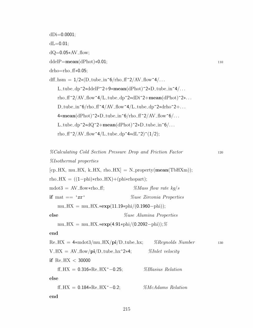
dDi=0.0001;
dL=0.01;
dQ=0.05∗AV flow;
ddelP=mean(dPhot)∗0.01; 110
drho=rho ff∗0.05;
dff hsm = 1/2∗(D tube in^6/rho ff^2/AV flow^4/. . .
L tube dp^2∗ddelP^2+9∗mean(dPhot)^2∗D tube in^4/. . .
rho ff^2/AV flow^4/L tube dp^2∗dDi^2+mean(dPhot)^2∗. . .
D tube in^6/rho ff^4/AV flow^4/L tube dp^2∗drho^2+. . .
4∗mean(dPhot)^2∗D tube in^6/rho ff^2/AV flow^6/. . .
L tube dp^2∗dQ^2+mean(dPhot)^2∗D tube in^6/. . .
rho ff^2/AV flow^4/L tube dp^4∗dL^2)^(1/2);
%Calculating Cold Section Pressure Drop and Friction Factor 120
%Isothermal properties
[cp HX, mu HX, k HX, rho HX] = N property(mean(TbHXm));
rho HX = ((1−phi)∗rho HX)+(phi∗rhopart);
mdot3 = AV flow∗rho ff; %Mass flow rate kg/s
if mat == 'zr' %use Zirconia Properties
mu HX = mu HX.∗exp(11.19∗phi/(0.1960−phi));
else %use Alumina Properties
mu HX = mu HX.∗exp(4.91∗phi/(0.2092−phi));%
end
Re HX = 4∗mdot3/mu HX/pi/D tube hx; %Reynolds Number 130
V HX = AV flow/pi/D tube hx^2∗4; %Inlet velocity
if Re HX < 30000
ff HX = 0.316∗Re HX^−0.25; %Blasius Relation
else
ff HX = 0.184∗Re HX^−0.2; %McAdams Relation
end
215

delPhx = ff HX∗L tube dp/D tube hx∗rho HX∗V HX^2/2; %Delta P in Pa
%Measured friction factor 140
ff HXm = mean(dPcold)∗6894.75728∗D tube hx/. . .
L tube dp∗2/rho HX/V HX^2;
dDi=0.0001;
dL=0.01;
dQ=0.05∗AV flow;
ddelP=mean(dPcold)∗0.01;
drho=rho HX∗0.05;
dff HX = 1/2∗(D tube hx^6/rho HX^2/AV flow^4/L tube dp^2∗. . .
ddelP^2+9∗mean(dPcold)^2∗D tube hx^4/rho HX^2/. . .
AV flow^4/L tube dp^2∗dDi^2+mean(dPcold)^2∗. . . 150
D tube hx^6/rho HX^4/AV flow^4/L tube dp^2∗drho^2+. . .
4∗mean(dPcold)^2∗D tube hx^6/rho HX^2/AV flow^6/. . .
L tube dp^2∗dQ^2+mean(dPcold)^2∗D tube hx^6/. . .
rho HX^2/AV flow^4/L tube dp^4∗dL^2)^(1/2);
%Prediction of Local Nusselt Number
z=xloc;
for i=1:14 %i=1:n
Tb(i) = (z(i)∗(Tboutm−(Tbinm))/L tube)+(Tbinm);
160
%local properties
[cp(i), mu(i), k(i), rho(i)] = N property(Tb(i));
%Setting Nanofluid Properties
cp(i) = (((1−phi)∗rho(i)∗cp(i))+(phi∗rhopart∗cppart))/. . .
(((1−phi)∗rho(i))+(phi∗rhopart));
216

rho(i) = ((1−phi)∗rho(i))+(phi∗rhopart);
if mat == 'zr' %use Zirconia Properties
mu(i) = mu(i).∗exp(11.19∗phi/(0.1960−phi)); 170
k(i) = k(i).∗ (−29.867∗phi^2 + 2.4505∗phi + 1);
else %use Alumina Properties
mu(i) = mu(i).∗exp(4.91∗phi/(0.2092−phi)); %
k(i) = k(i).∗ (4.5503∗phi + 1); %
end
Re(i) = 4∗rho(i)∗AV flow/mu(i)/pi/D tube in; %local Reynolds
Pr(i) = mu(i)∗cp(i)∗1000/k(i); %local Prandtl
%Calculating Friction Factor for Gnielinski
ff(i) = (0.790∗log(Re(i))−1.64)^−2; 180
%Calculating Nusselt Number for Gnielinski
Nu(i) = (ff(i)/8)∗(Re(i)−1000)∗Pr(i)/(1+12.7∗. . .
((ff(i)/8)^(1/2))∗(Pr(i)^(2/3)−1));. . .
%∗(1+(D tube in/L tube)^(2/3));
%Calculating Nusselt Number for Dittus Boelter
NuDB(i)=0.023∗Re(i)^0.8∗Pr(i)^0.4;
htc(i) = Nu(i)∗k(i)/D tube in; %local heat transfer coeff.
Tw(i) = (q flux/htc(i))+Tb(i); %local wall temperature
kw(i)= 0.0127∗(Tw(i))+13.23188; %Temp Dep Wall Conductivity
Two(i)=Tw(i)+Power/(2∗pi∗kw(i)∗L tube)∗(D tube out^2/. . . 190
(D tube out^2−D tube in^2)∗log(D tube out/. . .
D tube in)−1/2); %local outer wall temperature
dTwall(i)=Two(i)−Tw(i);
end
%Correcting Wall Temperature for Conduction
217

Twinn=Tm−dTwall;
%Calculating Local Measured Heat Transfer Coefficient
for ii=1:14 200
htcmeas(ii)=q flux/(Twinn(ii)−(Tb(ii)));
%local properties
[cp2(ii), mu2(ii), k2(ii), rho2(ii)] = N property(Tb(ii));
Numeas(ii)=htcmeas(ii)∗D tube in/(k2(ii));
%Uncertainty Analysis for Local HTC and Nusselt
cp2(ii)=cp2(ii)∗1000;
dI=0.08; 210
dV=0.004;
dL=0.01;
dTwo=0.5;
dkw=1;
dcp=100;
dDi=0.0001;
dDo=0.0001;
dTin=0.5;
htcerror(ii) = 1/2∗(4/(Twinn(ii)−Tb(ii))^2∗(Vm^2/pi^2/. . . 220
D tube in^2/L tube^2∗dI^2+Im^2/pi^2/D tube in^2/. . .
L tube^2∗dV^2+Im^2∗Vm^2/pi^2/D tube in^4/L tube^2∗. . .
dDi^2+Im^2∗Vm^2/pi^2/D tube in^2/L tube^4∗dL^2)+. . .
q flux^2/(Twinn(ii)−Tb(ii))^4∗(4∗dTwo^2+Vm^2/. . .
pi^2/kw(ii)^2/L tube^2∗(D tube out^2/. . .
(D tube out^2−D tube in^2)∗log(D tube out/. . .
218

D tube in)−1/2)^2∗dI^2+Im^2/pi^2/kw(ii)^2/. . .
L tube^2∗(D tube out^2/(D tube out^2−D tube in^2)∗. . .
log(D tube out/D tube in)−1/2)^2∗dV^2+Im^2∗Vm^2/. . .
pi^2/kw(ii)^4/L tube^2∗(D tube out^2/. . . 230
(D tube out^2−D tube in^2)∗log(D tube out/. . .
D tube in)−1/2)^2∗dkw^2+Im^2∗Vm^2/pi^2/kw(ii)^2/. . .
L tube^4∗(D tube out^2/(D tube out^2−D tube in^2)∗. . .
log(D tube out/D tube in)−1/2)^2∗dL^2+Im^2∗. . .
Vm^2/pi^2/kw(ii)^2/L tube^2∗(2∗D tube out/. . .
(D tube out^2−D tube in^2)∗log(D tube out/. . .
D tube in)−2∗D tube out^3/(D tube out^2−. . .
D tube in^2)^2∗log(D tube out/D tube in)+. . .
D tube out/(D tube out^2−D tube in^2))^2∗. . .
dDo^2+Im^2∗Vm^2/pi^2/kw(ii)^2/L tube^2∗. . . 240
(2∗D tube out^2/(D tube out^2−D tube in^2)^2∗. . .
log(D tube out/D tube in)∗D tube in−D tube out^2/. . .
(D tube out^2−D tube in^2)/D tube in)^2∗dDi^2)+. . .
4∗q flux^2/(Twinn(ii)−Tb(ii))^4∗(Vm^2/rho2(ii)^2/. . .
AV flow^2/cp2(ii)^2∗dI^2+Im^2/rho2(ii)^2/. . .
AV flow^2/cp2(ii)^2∗dV^2+Im^2∗Vm^2/rho2(ii)^2/. . .
AV flow^2/cp2(ii)^4∗dcp^2+dTin^2))^(1/2);
dNu(ii) =(D tube in^2/k2(ii)^2∗htcerror(ii)^2+. . . 250
htcmeas(ii)^2/k2(ii)^2∗dDi^2+htcmeas(ii)^2∗. . .
D tube in^2/k2(ii)^4∗(k2(ii)∗0.05)^2)^(1/2);
end
avedata(ij,1:23)=[phi,Qm∗0.00006309,Tbinm,Tboutm,. . .
219

q flux,mean(Re),Re HX,mean(NuDB),mean(Numeas),. . .
delPhs,mean(dPhot)∗6894.75728,delPhx,mean(dPcold)∗. . .
6894.75728, ff hs, ff hsm, dff hsm, ff HX, ff HXm,. . .
dff HX,mean(htcmeas), mean(Pr),mean(htcerror),mean(dNu)]; 260
nuout(ij,1:42)=[NuDB,Numeas,dNu]
Mats(ij,1:2)=mat;
DD1='mats';'phi';'QmL/s';'Tbinm';'Tb_out';'q_flux';. . .
'Re';'Re_HX';'Nu';'Numeas';'delP';'dPhot';'delPhx';. . .
'dPcold';'ffhot';'ffhotm';'dff_hot';'ffhx';'ffhxm';. . .
'dff_hx';'htcmeas'; 'Pr';'htcerror';'Nuerror'
XLSWRITE('ALL.xls',DD1','A1:X1') 270
XLSWRITE('ALL.xls',Mats,'A2:A48')
XLSWRITE('ALL.xls',avedata,'B2:X48')
D.2 Properties Program
function [cp1, mu1, k1, rho1]=N property(T1)
%Returns Water properties for pressure of
%0.1MPa (1bars) and temps from 290 to 453K
%Temperature
T=[280 282.5 285 287.5 290 292.5 295 297.5 300 . . .
302.5 305 307.5 310 312.5 315 317.5 320 322.5. . .
325 327.5 330 332.5 335 337.5 340 342.5 345.0. . .
347.5 350 352.5 355 357.5 360 362.5 365 367.5. . .
220

370 372.5 375 377.5 380 382.5 385 387.5 390.0. . . 10
392.5 395 397.5 400 402.5 405 407.5 410 412.5. . .
415 417.5 420 422.5 425 427.5 430 432.5 435.0. . .
437.5 440 442.5 445 447.5 450 452.5 453.03];
%Specific Heat Capacity
cp=[4.1973 4.1928 4.1891 4.1861 4.1836 4.1817 4.1802. . .
4.179 4.1781 4.1775 4.1771 4.177 4.177 4.1771. . .
4.1774 4.1779 4.1784 4.1791 4.1798 4.1807 4.1816. . .
4.1827 4.1838 4.185 4.1863 4.1877 4.1892 4.1908. . .
4.1925 4.1943 4.1962 4.1982 4.2004 4.2026 4.205. . . 20
4.2075 4.2101 4.2129 4.2158 4.2188 4.222 4.2254. . .
4.2289 4.2325 4.2364 4.2404 4.2446 4.2489 4.2535. . .
4.2582 4.2632 4.2683 4.2737 4.2792 4.285 4.291. . .
4.2972 4.3037 4.3104 4.3173 4.3245 4.332 4.3397. . .
4.3478 4.3561 4.3647 4.3736 4.3829 4.3924 4.4023. . .
4.4045];
cp1=interp1(T,cp,T1); % kJ/kg-K
%Viscosity 30
mu=[0.0014323 0.0013296 0.0012384 0.0011567 0.0010834. . .
0.0010173 0.00095752 0.00090319 0.00085367. . .
0.0008084 0.00076689 0.00072874 0.00069357. . .
0.00066109 0.00063101 0.00060311 0.00057717. . .
0.00055301 0.00053047 0.00050941 0.00048969. . .
0.00047121 0.00045386 0.00043755 0.00042221. . .
0.00040774 0.00039409 0.0003812 0.00036902. . .
0.00035748 0.00034655 0.00033619 0.00032635. . .
0.000317 0.00030811 0.00029966 0.0002916. . .
221

0.00028392 0.0002766 0.0002696 0.00026293. . . 40
0.00025654 0.00025043 0.00024459 0.00023899. . .
0.00023362 0.00022847 0.00022354 0.0002188. . .
0.00021424 0.00020986 0.00020565 0.0002016. . .
0.0001977 0.00019394 0.00019031 0.00018682. . .
0.00018345 0.0001802 0.00017705 0.00017402. . .
0.00017108 0.00016824 0.0001655 0.00016284. . .
0.00016026 0.00015776 0.00015534 0.00015299. . .
0.00015072 0.00015024];
mu1=interp1(T,mu,T1); %kg/m-s= Pa S 50
%Thermal Conductivity
k=[0.57454 0.57926 0.58395 0.5886 0.59319 0.59771. . .
0.60215 0.60649 0.61073 0.61485 0.61886 0.62274. . .
0.6265 0.63012 0.6336 0.63695 0.64016 0.64323. . .
0.64617 0.64897 0.65164 0.65418 0.65658 0.65886. . .
0.66102 0.66306 0.66498 0.66679 0.66848 0.67008. . .
0.67156 0.67295 0.67424 0.67544 0.67655 0.67758. . .
0.67852 0.67937 0.68015 0.68086 0.68149 0.68204. . .
0.68253 0.68295 0.68331 0.6836 0.68383 0.68399. . . 60
0.6841 0.68415 0.68414 0.68407 0.68395 0.68377. . .
0.68353 0.68325 0.6829 0.68251 0.68206 0.68156. . .
0.681 0.68039 0.67973 0.67902 0.67825 0.67743. . .
0.67655 0.67562 0.67464 0.6736 0.67337];
k1=interp1(T,k,T1); %W/m-K
%Density
rho=[1000.3 1000.2 999.94 999.62 999.22 998.75 998.22. . .
222

997.62 996.96 996.24 995.47 994.65 993.78. . . 70
992.86 991.89 990.88 989.82 988.72 987.58. . .
986.4 985.18 983.92 982.63 981.3 979.93. . .
978.53 977.1 975.63 974.13 972.6 971.03. . .
969.44 967.81 966.16 964.47 962.75 961.01. . .
959.24 957.43 955.6 953.74 951.86 949.94. . .
948 946.03 944.03 942.01 939.95 937.87 935.77. . .
933.63 931.47 929.28 927.06 924.82 922.54. . .
920.24 917.92 915.56 913.17 910.76 908.32. . .
905.85 903.34 900.81 898.25 895.66 893.04. . .
890.39 887.7 887.13]; 80
rho1=interp1(T,rho,T1); %kg/m3
223

224

Appendix E
Raw data from convection
experiments
225

00H2hit 00H2hitm 00H2lit 00H2litm 00H2mit 00H2mitmFlowrate (GPM) 3.00494 2.1733 3.06269 2.13876 2.97037 2.16391Voltage (V) 18.67278 18.65394 17.91732 18.02414 18.18814 18.32702Current (A) 464.9508 464.9247 465.0416 464.9816 464.9652 464.9612Bulk Inlet Temperature(C) 64.98971 60.50614 22.64198 24.30401 37.69999 41.749750.2m Wall Temperature(C) 76.92643 74.53683 36.27494 40.7199 50.61591 56.746140.4m Wall Temperature(C) 77.40044 75.23674 36.68983 41.40102 51.06766 57.439180.6m Wall Temperature(C) 78.83917 76.96001 38.16023 43.15039 52.55827 59.18280.8m Wall Temperature(C) 79.15557 77.52691 38.28732 43.55246 52.75612 59.674581.0m Wall Temperature(C) 80.94446 79.58568 40.17383 45.74737 54.62481 61.774691.2m Wall Temperature(C) 81.26407 80.17421 40.35535 46.22822 54.88095 62.311031.4m Wall Temperature(C) 82.19233 81.37135 41.11659 47.28383 55.72038 63.421.6m Wall Temperature(C) 82.23067 81.67714 41.05945 47.50468 55.72001 63.678231.8m Wall Temperature(C) 82.72624 82.43108 41.54454 48.25346 56.23802 64.445542.0m Wall Temperature(C) 83.80283 83.77626 42.60747 49.60364 57.3328 65.795922.2m Wall Temperature(C) 85.14393 85.38461 43.89806 51.15237 58.67855 67.393162.4m Wall Temperature(C) 85.38755 85.89222 43.85421 51.39443 58.762 67.763052.6m Wall Temperature(C) 86.10437 86.91915 44.41232 52.33759 59.39135 68.742772.8m Wall Temperature(C) 86.31836 87.2639 44.96249 53.29815 59.81508 69.30712Bulk Outlet Temperature(C) 75.65207 75.07867 32.62207 38.82036 48.16604 56.23373HX Outlet Temperature(C) 64.9397 60.51187 21.94953 23.3907 37.24079 41.24327Isothermal DP (psi) 2.39482 1.40159 2.98065 1.57596 2.6123 1.49122Heated DP (psi) 3.12986 1.78977 3.79768 1.95215 3.36358 1.89096System Pressure (psi) 5.856 4.45594 3.2521 3.12283 3.66034 3.33701
Figure E-1: Water
09Al2gpm23 09A3gpm21 09A3gpm27hhf 09A3gpm39 09A3gpm63Flowrate (GPM) 2.14708 3.71554 3.85107 3.59714 3.57432Voltage (V) 18.0176 17.86031 24.30109 18.17284 18.61698Current (A) 464.10529 464.11328 620.27004 464.11436 464.05445Bulk Inlet Temperature(C) 22.82405 21.43268 27.8986 38.80434 63.80740.2m Wall Temperature(C) 40.76522 34.75831 50.42508 51.13973 75.076170.4m Wall Temperature(C) 41.40868 35.05696 50.90551 51.46299 75.448230.6m Wall Temperature(C) 43.19123 36.43843 53.27517 52.79873 76.79550.8m Wall Temperature(C) 43.75072 36.57545 53.55975 53.14741 77.364951.0m Wall Temperature(C) 46.0893 38.39788 56.81484 54.96446 79.112241.2m Wall Temperature(C) 46.55323 38.48939 56.94746 55.12178 79.355141.4m Wall Temperature(C) 47.56636 39.15593 58.16805 55.88185 80.190081.6m Wall Temperature(C) 47.92721 39.02766 57.88674 55.81818 80.194621.8m Wall Temperature(C) 48.74881 39.46218 58.62015 56.25802 80.575662.0m Wall Temperature(C) 50.20709 40.51077 60.45831 57.3158 81.59862.2m Wall Temperature(C) 51.75584 41.67084 62.44647 58.4985 82.733562.4m Wall Temperature(C) 51.97254 41.4593 62.17147 58.47775 82.977192.6m Wall Temperature(C) 53.11035 42.05278 63.14805 59.12915 83.674162.8m Wall Temperature(C) 54.02716 42.47715 63.81264 59.36877 83.61638Bulk Outlet Temperature(C) 38.17461 30.08651 43.2501 47.88912 73.13351HX Outlet Temperature(C) 21.32882 20.52 27.07865 38.21521 63.59562Isothermal DP (psi) 1.54749 4.10802 4.2043 3.5532 3.16486Heated DP (psi) 1.8819 5.15152 5.13625 4.52001 4.12396System Pressure (psi) 3.02007 3.7945 4.4923 4.33714 6.10408
Figure E-2: Nyacol Alumina 0.9 vol%
226

18Al2gpm26 18Al3gpm21 18Al3gpm27mhf 18Al3gpm33hhf 18Al3gpm36 18Al3gpm60Flowrate (GPM) 2.11176 3.48637 3.71442 3.75559 3.60543 3.67032Voltage (V) 18.08459 17.87957 20.86823 24.45347 18.12009 18.5501Current (A) 464.11617 464.13844 535.851 620.21515 464.10945 464.09721Bulk Inlet Temperature(C) 25.91971 21.40127 27.78721 33.40198 35.52497 60.212450.2m Wall Temperature(C) 44.47903 35.50469 45.57036 56.4685 48.46948 71.855180.4m Wall Temperature(C) 45.14299 35.81661 45.95874 56.96888 48.78125 72.180620.6m Wall Temperature(C) 46.9389 37.18 47.78777 59.4234 50.10509 73.472210.8m Wall Temperature(C) 47.51333 37.35651 47.99497 59.7354 50.44356 74.011961.0m Wall Temperature(C) 49.80852 39.1952 50.45109 62.99287 52.27215 75.788331.2m Wall Temperature(C) 50.26745 39.27104 50.55818 63.15393 52.393 75.979451.4m Wall Temperature(C) 51.26199 39.9389 51.41532 64.2907 53.0932 76.741031.6m Wall Temperature(C) 51.6144 39.8526 51.27172 64.09842 53.04206 76.709141.8m Wall Temperature(C) 52.43639 40.30477 51.83576 64.84272 53.47838 77.09182.0m Wall Temperature(C) 53.91524 41.35752 53.22519 66.70695 54.52115 78.111552.2m Wall Temperature(C) 55.45943 42.51129 54.69912 68.67211 55.67583 79.209072.4m Wall Temperature(C) 55.68051 42.31299 54.51399 68.51639 55.61823 79.384522.6m Wall Temperature(C) 56.83478 42.93003 55.29438 69.52188 56.24698 80.043752.8m Wall Temperature(C) 57.45348 43.26892 55.94786 70.22168 56.48817 80.12054Bulk Outlet Temperature(C) 41.28559 30.25747 39.45859 49.1903 44.43941 69.20803HX Outlet Temperature(C) 24.51621 20.52037 26.91552 32.6007 34.8257 59.78618Isothermal DP (psi) 1.66467 4.34893 4.37949 4.301 4.03712 3.70054Heated DP (psi) 2.02193 5.40871 5.42377 5.25433 5.10331 4.77444System Pressure (psi) 3.16892 3.91395 5.19716 5.53237 4.62547 6.7149
Figure E-3: Nyacol Alumina 1.8 vol%
36Al2gpm24 36Al3gpm24 36Al3gpm39hhf 36Al3gpm41 36Al3gpm59Flowrate (GPM) 2.1384 3.28003 3.34814 3.36738 3.38854Voltage (V) 18.10837 18.02803 24.70353 18.3139 18.61091Current (A) 464.13476 465.12444 620.23816 465.07781 465.11957Bulk Inlet Temperature(C) 23.68641 24.24426 39.0955 41.51349 59.2340.2m Wall Temperature(C) 45.98109 41.30078 65.87838 56.5571 72.748250.4m Wall Temperature(C) 46.62167 41.65096 66.46589 56.92535 73.10190.6m Wall Temperature(C) 48.29552 43.1406 69.02002 58.43503 74.53170.8m Wall Temperature(C) 48.7223 43.23788 69.40198 58.59802 75.001211.0m Wall Temperature(C) 50.97775 45.20934 72.8344 60.48918 76.815311.2m Wall Temperature(C) 51.21864 45.28686 73.01497 60.6322 77.019191.4m Wall Temperature(C) 52.15632 45.96563 74.24088 61.34251 77.762431.6m Wall Temperature(C) 52.43409 45.96144 74.16273 61.37967 77.831241.8m Wall Temperature(C) 53.13548 46.48248 75.00669 61.87477 78.287362.0m Wall Temperature(C) 54.58645 47.62865 76.96351 62.96377 79.357712.2m Wall Temperature(C) 56.00161 48.78805 79.00559 64.14473 80.522882.4m Wall Temperature(C) 56.0483 48.64737 78.9349 64.17745 80.714392.6m Wall Temperature(C) 57.21147 49.37382 80.14265 64.88371 81.443062.8m Wall Temperature(C) 57.70733 49.6353 80.58697 65.02226 81.46818Bulk Outlet Temperature(C) 38.62886 34.05324 56.74525 51.24416 68.89603HX Outlet Temperature(C) 22.43631 23.29163 38.44172 40.81704 58.87414Isothermal DP (psi) 2.20866 4.51088 4.33627 4.27541 4.06223Heated DP (psi) 2.61975 5.53466 5.195 5.365 5.17097System Pressure (psi) 3.2164 4.10653 5.18645 4.95686 6.48639
Figure E-4: Nyacol Alumina 3.6 vol%
227

00H22gpm20 00H22gpm40 00H22gpm60 00H23gpm20 00H23gpm40 00H23gpm60 00H24gpm20Flowrate (GPM) 2.08034 2.07694 2.09386 3.10176 3.21777 3.23872 3.89877Voltage (V) 18.24232 18.57912 18.87757 18.00325 18.37696 18.81143 18.0497Current (A) 468.25321 468.56675 468.54142 465.61421 466.04022 468.22107 468.44613Bulk Inlet Temperature(C) 27.32241 45.8845 62.92734 24.47138 44.98746 64.61695 24.221740.2m Wall Temperature(C) 44.1826 61.33645 77.51302 38.19707 57.47591 76.4671 36.651910.4m Wall Temperature(C) 44.74066 61.97111 78.19125 38.4462 57.77038 76.80705 36.741380.6m Wall Temperature(C) 46.53326 63.71944 79.93023 39.82951 59.16999 78.18583 38.052570.8m Wall Temperature(C) 47.00199 64.26776 80.59293 40.04607 59.39551 78.47973 38.063611.0m Wall Temperature(C) 49.31427 66.56999 82.83967 42.03153 61.27546 80.29592 39.861.2m Wall Temperature(C) 49.86361 67.20125 83.51283 42.28001 61.55684 80.6309 39.954951.4m Wall Temperature(C) 50.86178 68.29279 84.64904 43.03529 62.32196 81.47161 40.583961.6m Wall Temperature(C) 51.22542 68.69037 85.09655 43.00538 62.32548 81.50864 40.386741.8m Wall Temperature(C) 51.97732 69.4376 85.80699 43.45807 62.72522 81.84551 40.695752.0m Wall Temperature(C) 53.46722 70.9437 87.27752 44.62602 63.8416 82.92925 41.711092.2m Wall Temperature(C) 55.133 72.5897 88.92127 45.93997 65.10668 84.15208 42.854192.4m Wall Temperature(C) 55.31439 72.96352 89.48566 45.78854 65.12046 84.3421 42.556842.6m Wall Temperature(C) 56.54093 74.22485 90.83136 46.58874 65.91691 85.19349 43.155662.8m Wall Temperature(C) 57.23822 74.56683 91.01185 46.85744 66.04466 85.09607 43.84462Bulk Outlet Temperature(C) 42.28322 60.99272 78.16016 34.29705 54.7069 74.48383 31.92871HX Outlet Temperature(C) 25.84694 44.83203 62.48355 23.33225 44.22969 64.25673 23.25417Isothermal DP (psi) 1.50873 1.40297 1.32311 3.07505 2.96851 2.82873 4.7782Heated DP (psi) 1.88227 1.80357 1.74711 3.9096 3.89219 3.80983 6.21708System Pressure (psi) 2.50066 2.94688 4.19113 3.75889 3.81128 5.40596 4.45369
Figure E-5: Water Retest
02zr1gpm30 02zr2gpm28 02zr3gpm31 02zr3gpm37 02zr3gpm40 02zr3gpm63Flowrate (GPM) 1.05256 1.97399 3.23591 3.1776 3.14237 3.16477Voltage (V) 18.4147 18.11652 20.90937 24.58307 18.20876 18.60929Current (A) 463.69928 463.71248 534.60097 620.24427 463.72385 463.7209Bulk Inlet Temperature(C) 30.17757 28.4696 31.28818 37.23974 40.19891 63.109840.2m Wall Temperature(C) 57.2215 46.49989 49.27526 60.93604 53.32542 75.154060.4m Wall Temperature(C) 58.55154 47.07186 49.51524 61.29328 53.58902 75.501460.6m Wall Temperature(C) 61.12441 48.84714 51.36509 63.81432 54.97188 76.885960.8m Wall Temperature(C) 62.34489 49.34029 51.547 64.07715 55.17022 77.145711.0m Wall Temperature(C) 65.62477 51.68875 54.0838 67.51872 57.09922 78.948521.2m Wall Temperature(C) 66.96229 52.26187 54.32547 67.87998 57.35114 79.253081.4m Wall Temperature(C) 68.7517 53.26052 55.22238 69.14545 58.0882 80.07441.6m Wall Temperature(C) 70.16564 53.72072 55.21901 69.14262 58.13158 80.159011.8m Wall Temperature(C) 71.86951 54.59493 55.86004 70.0307 58.61864 80.582342.0m Wall Temperature(C) 74.29244 56.12319 57.34452 72.03663 59.7537 81.681942.2m Wall Temperature(C) 76.79373 57.75138 58.96564 74.21324 60.97549 82.894622.4m Wall Temperature(C) 78.04988 58.05067 58.84657 74.17127 60.9911 83.111072.6m Wall Temperature(C) 80.40835 59.31915 59.82354 75.48213 61.78248 83.961162.8m Wall Temperature(C) 81.30343 59.99526 60.42169 76.10372 61.90623 83.78941Bulk Outlet Temperature(C) 61.00621 44.46611 44.1889 55.14908 50.14591 73.09134HX Outlet Temperature(C) 28.24339 27.21569 30.4717 36.55966 39.5335 62.9157Isothermal DP (psi) 0.4523 1.36003 3.20483 3.022 2.92607 2.73728Heated DP (psi) 0.51691 1.69306 4.02602 3.7604 3.7737 3.62362System Pressure (psi) 3.95199 4.50467 5.45377 5.60087 5.41823 7.29462
Figure E-6: Nyacol Zirconia 0.2 vol%
228

05zr1gpm28 05zr2gpm30 05zr3gpm28 05zr3gpm33mhf 05zr3gpm39hhf 05zr3gpm40 05zr3gpm60Flowrate (GPM) 1.01515 2.06051 3.55744 3.46943 3.46132 3.38666 3.47349Voltage (V) 18.44775 18.1832 18.01022 21.1347 24.57007 18.22731 18.57796Current (A) 463.71327 464.57508 464.59571 539.60519 619.19776 464.54747 464.54Bulk Inlet Temperature(C) 29.14622 30.08693 28.23168 32.5862 39.18418 39.60241 59.96040.2m Wall Temperature(C) 58.72072 48.57727 42.02161 50.9954 62.73373 52.96708 72.244530.4m Wall Temperature(C) 60.14585 49.11654 42.15548 51.1709 62.97651 53.20181 72.493830.6m Wall Temperature(C) 62.68138 50.8881 43.51732 53.01383 65.41311 54.55386 73.825120.8m Wall Temperature(C) 63.89634 51.31437 43.57759 53.137 65.58519 54.70904 74.042971.0m Wall Temperature(C) 67.29677 53.66815 45.4835 55.68788 68.9421 56.61359 75.819081.2m Wall Temperature(C) 68.57766 54.20186 45.60701 55.88687 69.22975 56.82178 76.054281.4m Wall Temperature(C) 70.39178 55.18459 46.24088 56.76519 70.43198 57.52937 76.792891.6m Wall Temperature(C) 71.82577 55.61827 46.17488 56.70418 70.32653 57.52046 76.826071.8m Wall Temperature(C) 73.50875 56.44731 46.6112 57.29168 71.09794 57.98448 77.220212.0m Wall Temperature(C) 75.99534 57.95644 47.68889 58.76514 73.0321 59.08851 78.282662.2m Wall Temperature(C) 78.559 59.54968 48.84696 60.3299 75.10884 60.29639 79.47442.4m Wall Temperature(C) 79.73114 59.81972 48.67653 60.19639 74.98602 60.2583 79.613382.6m Wall Temperature(C) 82.18225 61.03666 49.35125 61.12081 76.20742 61.00588 80.409052.8m Wall Temperature(C) 82.9009 61.62327 49.84904 61.55225 76.5203 61.1323 80.42511Bulk Outlet Temperature(C) 61.32544 45.76329 37.15283 45.05494 55.9053 49.10197 69.35842HX Outlet Temperature(C) 27.11743 28.85878 27.37513 31.78973 38.51185 38.96035 59.67277Isothermal DP (psi) 0.44587 1.4817 3.9422 3.69677 3.5525 3.37605 3.22988Heated DP (psi) 0.4973 1.84638 5.01236 4.63281 4.42264 4.33112 4.23807System Pressure (psi) 3.78214 4.56177 5.85873 5.88841 6.10362 5.4729 7.67655
Figure E-7: Nyacol Zirconia 0.5 vol%
09zr2gpm38 09zr3gpm31 09zr3gpm43 09zr3gpm50hhf 09zr3gpm60Flowrate (GPM) 2.03722 3.1855 3.24266 3.21843 3.22712Voltage (V) 18.33887 18.18921 18.38689 24.9098 18.67438Current (A) 464.54793 466.6289 466.55435 620.21681 466.5743Bulk Inlet Temperature(C) 38.50456 31.62775 43.27469 50.74866 59.897720.2m Wall Temperature(C) 57.31303 46.94986 57.53344 75.00809 73.13060.4m Wall Temperature(C) 57.83732 47.1713 57.78243 75.40258 73.42120.6m Wall Temperature(C) 59.57504 48.53944 59.13909 77.89033 74.743780.8m Wall Temperature(C) 59.99302 48.67307 59.32288 78.08654 74.974091.0m Wall Temperature(C) 62.24657 50.61906 61.19756 81.46148 76.798031.2m Wall Temperature(C) 62.72564 50.78759 61.3865 81.76794 77.031631.4m Wall Temperature(C) 63.65355 51.42463 62.05961 82.965 77.762341.6m Wall Temperature(C) 64.05099 51.42881 62.07173 82.90725 77.812561.8m Wall Temperature(C) 64.79118 51.85876 62.49017 83.67201 78.210782.0m Wall Temperature(C) 66.24901 52.97754 63.58277 85.62261 79.276632.2m Wall Temperature(C) 67.77864 54.18317 64.78637 87.73328 80.475532.4m Wall Temperature(C) 68.03752 54.02866 64.72866 87.68329 80.582132.6m Wall Temperature(C) 69.26795 54.82585 65.52694 89.00783 81.428332.8m Wall Temperature(C) 69.62152 54.94236 65.5634 89.10601 81.19179Bulk Outlet Temperature(C) 53.45984 41.16436 52.75321 67.86288 69.44882HX Outlet Temperature(C) 37.52995 30.81392 42.64694 50.24725 59.56394Isothermal DP (psi) 1.73875 3.94456 3.81485 3.70913 3.55899Heated DP (psi) 2.17511 4.97116 4.88016 4.62221 4.61825System Pressure (psi) 4.0351 4.02895 4.97184 5.91178 6.31908
Figure E-8: Nyacol Zirconia 0.9 vol%
229

230

Appendix F
Theoretical Investigation of Gas
Nanofluids
Gas nanofluids are of interest to nuclear engineers from the standpoint of advanced
gas reactor cooling like the gas cooled fast reactor (GFR) or the high temperature
gas cooled reactor (HTGR). Gas nanofluids are also of great interest in fusion reactor
divertor cooling. As a part of the current LDRD project, Idaho National Lab (INL)
has taken the lead in the design and construction of a gas-nanoparticle suspension
convective cooling experiment as shown in Figure F-1. This chapter will cover some
initial theoretical background work on gas-particulate flows which are done to help
guide the experimental and future theoretical investigations of gas nanofluids.
The author spent a 3-week period at INL in 2005 and contributed this work to
the gas nanofluid project underway there. A determination of the key transport
phenomena in the INL gas nanofluid experiment is made through a semi-quantitative
approach. The current specifications of the experiment (i.e., temperature, pressure,
flow, ID, etc.) are used in the analysis. It is important to note that, due to the
sensitivity of gas properties to temperature and pressure, gas nanofluid systems can
be regarded as continuous, free molecular, or transitional in behavior; thus the results
of this analysis are applicable to the described experimental situation only. The
insights found lead to the recommendation of certain focal points for the experimental
and future theoretical work with gas nanofluids. This chapter is divided into three
231

Figure F-1: INL gas loop experiment schematic
sections: Assumptions, Analysis, and Recommendations.
F.1 Assumptions
The main assumption is that the flow situation considered is for the INL gas nanofluid
experiment. The experiment is a once-through heated pipe convection heat transfer
system. The system has the means to inject, measure, and remove nanometer sized
particles at various concentrations. The purpose of the experiment is to determine
the potential for using gas nanoparticle dispersions (nanofluids) to enhance convective
heat transfer. The experiment uses helium gas as the base fluid and, for the sake of
analysis, carbon based nanoparticles. For the analysis the following parameters are
set:
Helium Gas State and Properties
• Pressure (P ) = 0.2 MPa
232

• Temperature (T ) = 873 K
• Viscosity (µ) ≈ 4x10⁻⁵ Pa-s
• Thermal Conductivity (k) ≈ 0.3 W/m-K
• Density (ρ) ≈ 0.11 kg/m3
• Heat Capacity (c) ≈ 5193 J/kg-K
• Ideal Gas Constant (R) = 8.31 J/mol-K
• Avogadro’s Number (Nav) = 6.022x10²³ atoms/mol
• Effective diameter of single molecule (dHe) ≈ 0.6x10⁻¹⁰ m
Nanoparticle Properties
• Material - Pyro-carbon Spheres
• Particle Diameter (dp) = 1-100 nm
• Thermal Conductivity (kp) ≈ 4 W/m-K or greater
• Density (ρp) ≈ 1900 kg/m3
• Heat Capacity (cp] ≈ 709 J/kg-K
Operating conditions
• Reynolds Number (Re) = 4000
• Pipe diameter (D) = 17.3 mm
F.2 Analysis
The analysis is composed of five parts as follows: 1) assessment of the continuum as-
sumption, 2) evaluation of the internal particle temperature response, 3) evaluation
233

of the particle/fluid heat transfer response, 4) evaluation of nanoparticle dispersion
and turbulence intensification as heat transfer enhancement mechanisms, and 5) dis-
cussion of other possible heat transfer enhancement mechanisms.
F.2.1 Continuum Assumption
The common way of determining whether the fluid-particle interaction can be treated
as a continuum phenomenon or not is to calculate the Knudsen number (Kn). The
Knudsen number is the ratio of the mean free path (λ) of the fluid particles to the
characteristic length of the system with which they interact. Here it is the mean free
path of the gas atoms divided by the diameter of the nanoparticles as shown:
Kn = λ/dp (F.1)
λ =RT√
2πdHePNav
(F.2)
Knudsen values less than 0.01 are considered to be in the continuum; values from
0.01 to 1.0 can be considered near-continuum; values from 1.0 to 10 can be consid-
ered transitional; values above 10 are free molecular. Navier-Stokes equations are
valid for the continuum regime below 0.01 and can be extended, through the use of
slip conditions, up to 0.1. Figure F-2 shows the dependence of the Knudsen num-
ber on the diameter of the nanoparticle. From the figure, it is determined that the
nanoparticle will see the surrounding gas as a free molecular interaction and therefore
not a continuum. However, at lower temperatures and higher pressures, the latter
being typical of gas-cooled reactor applications, the interaction is moved to the tran-
sitional regime. Other analysis determined the Knudsen number to be very weakly
dependent on the base gas.
234

dp (nm)
Kn
Figure F-2: Knudsen number for nanoparticles in helium gas
235

F.2.2 Determination of internal particle temperature response
A comparison of the time scale (τp) of energy redistribution within the nanoparticle
and the timescales of the energy transfer from the particle to the surrounding gas
determines whether the temperature distribution inside the nanoparticle can be re-
garded as uniform. Energy is transferred to and from the particle by conduction and
radiation, their time scales being indicated here as (τcon) and (τrad), respectively.
Energy redistribution within particle
The time scale of the energy transfer can be found as
τp ≈d2
p
αp · 0.12(F.3)
αp =kp
ρpcp
(F.4)
as shown from transient conduction solution for spherical systems with low Biot
number [76].
Heat conduction from particle to gas
An energy balance for the particle is developed as
ρpcpπ
6d3
p
dTp
dt= −π
2d2
png ckb(Tp − T ) (F.5)
where the right-hand term, the particle surface heat flux, is from Filippov and Ros-
ner’s paper [77], assuming an accommodation coefficient equal to one, γ = 5/3, and
T as the bulk gas temperature. It is also defined that
ng = (P ·Nav)/(R · T ) (F.6)
236

is the He atom concentration (atoms/m3) and
c =
√√√√8kbT
πng
(F.7)
is the average He atom speed and
ng = 0.004/Nav (F.8)
is the mass of a He atom (kg). From the energy balance equation, the time scale for
heat conduction to the gas is
τcon ≈ρpcpdp
3ng ckb
(F.9)
Heat radiation from particle to surroundings
An energy balance for the particle with radiation heat transfer is developed as
ρpcpπ
6d3
p
dTp
dt= −πd2
pσ(T 4p − T 4) (F.10)
(black body behavior is assumed) σ = 5.67 · 10−8 W/m2K4. From the energy balance
equation, the time scale for radiative heat transfer is
τrad ≈ρpcpdp
6σT 3(F.11)
Comparison of these time scales gives the relative importance of each mechanism in
the overall heat transfer process. Figure F-3 is a plot of the time scales of the three
mechanisms and how these vary with nanoparticle diameter.
Two conclusions can be drawn from Fig. F-3 : i) The energy redistribution within
the particle is much faster than the energy transfer between particle and gas due
to the large particle conductivity. Thus the temperature distribution within the
particle is uniform. ii) The dominant heat transfer mechanism from the particle to
the gas is conduction. However, due to its long-range nature, particle-to-particle and
particle-to-wall radiation can still play a significant role in the overall heat transfer
237

dp (nm)
τp
τcon
τrad
Figure F-3: Time scales for heat transfer mechanisms within and around nanoparticlesin helium gas
238

enhancement in the channel.
F.2.3 Determination of local thermal equilibrium between
the particles and the gas
A comparison of the time scale of the heat transfer from the particle to the gas
with the time scale of the particle slip motion in the gas can be used to determine
the thermal equilibrium characteristics of the mixture. The heat transfer time scale
has been determined above. In turbulent flow the dominant slip mechanism is from
inertial flight following the abrupt stop of an eddy. The time scale for this process is
the so-called relaxation time of the particle
τrel =ρpd
2p
18µCc (F.12)
and
Cc = 1 + Kn(α + βe−γ/Kn) (F.13)
is the Cunningham corrective factor, accounting for the non-continuum nature of the
particle/gas interaction. The coefficients α, β, and γ are determined experimentally
for exact fluid/particle combinations (which is not done here). For this calculation
the values α = 2.34, β = 1.05, and γ = -0.39 were assumed. It was later found from a
recent experiment of a similar system using polystyrene latex particles from 20nm to
270nm that α = 1.165, β = 0.483, and γ = 0.997 [78]. The Cunningham factors were
recalculated with these new values and found to be of the same order as the original
calculation. The time scales τrel and τcon are shown in Figure F-4. Since τcon τrel ,
it is concluded that particles can exchange energy very effectively as they fly within
the gas; therefore we can assume that there is local particle/gas thermal equilibrium.
239

dp (nm)
τcon
τrel
Figure F-4: Comparison of time scales for energy transfer and nanoparticle slip motionin helium gas
240

F.2.4 Heat transfer enhancement due to particle dispersion
and turbulence strengthening
Due to their small size, nanoparticles can be entrained in both large and small tur-
bulent eddies. This is shown by the size (l), velocity (V ) and time scales (τ) of the
eddies as follows:
Scales for large eddies:
• lo ∼ 0.07 ·D ∼ 1.2mm
• Vo ∼ Vshear ∼ 6m/s
• τo ∼ lo/Vo ∼ 2 · 10−4sec
Scales for small eddies (using Kolomogorov’s scaling laws):
• ls/lo ∼ Re−3/4 ⇒ ls ∼ 2.4µm
• τs/τo ∼ Re−1/2 ⇒ τs ∼ 3 · 10−6sec, Vs ∼ ls/τs ∼ 0.7m/s
It is seen that the particles (1-100nm) are much smaller than the eddy sizes (1.2mm
and 2.4µm).
The next step is to determine the stopping distance (S) for the particles entrained
in the small and large eddies in order to see how far they can be thrown by the eddy
velocities. It is found that
So =ρpd
2p
18µCcVo (F.14)
for particles entrained by large eddies and
Ss =ρpd
2p
18µCcVs (F.15)
for particles entrained by small eddies. The stopping distance is shown in Figure F-5.
Figure F-5 suggests that nanoparticles do not significantly project out of the eddies
with the possible exception of large nanoparticles, i.e., >100 nm, entrained by small
eddies. That is, the nanoparticles move with the turbulent eddies. Thus, contribution
241

dp (nm)
Ss
So
ℓs
ℓo
Figure F-5: Comparison of eddy sizes and particle stopping distances
242

of inertial slip to nanoparticle dispersion is probably negligible. Regarding the ques-
tion of turbulence intensification, the presence of the nanoparticles will likely increase
viscosity, which will delay the onset of turbulence for given mean velocity.
Moreover, Figure F-5 suggests that particles entrained by large eddies may interact
with (i.e., break up) small eddies, since their length scales are comparable. Based on
order-of-magnitude estimates of the kinetic energy carried by each eddy and using
Kolomogorov’s scaling laws, one finds that the ratio of the number of small eddies
generated per unit time and volume to the number of large eddies generated per
unit time and volume is proportional to Re11/4, which in our case is about 1010.
Therefore, small eddies are much more numerous than large eddies. This means that
nanoparticles being projected out of large eddies will affect only a very limited number
of small eddies. In summary, an effect on turbulence beyond the obvious effect via
the change in viscosity seems unlikely.
F.2.5 Other possible heat transfer enhancement mechanisms
At least three mechanisms remain possible and should be considered in future analysis:
1) thermal conductivity increase due to the presence of the nanoparticles
2) radiative heat transfer from particle to particle and from particle to wall
3) development of thermal conductivity and viscosity gradients, which can develop
in the boundary layer as a result of nanoparticle migration (e.g., phoretic effects,
shear-rate induced migration, etc.)
F.3 Recommendations
In view of the above considerations, the following recommendations are made for the
INL experiments:
a) Measure thermal conductivity and viscosity in static gas-particle systems,
b) Run a few experiments at temperatures for which the effect of radiation heat
transfer is expected to be small,
c) Attempt to measure nanoparticle concentration distribution in test section.
243

244

Bibliography
[1] A. El Ghzaoui. Measurement of the diffuse double-layer forces between zirconia
and α-alumina. Journal of Applied Physics, 86(10):5894–5897, 2006.
[2] Yimin Xuan and Qiang Li. Investigation on convective heat transfer and flow
features of nanofluids. Journal of Heat Transfer, 125(1):151–155, 2003. Com-
pilation and indexing terms, Copyright 2005 Elsevier Engineering Information,
Inc.
[3] J.C. Maxwell. Treatise on Electricity and Magnetism. Dover Publications, 1954.
[4] A.S. Ahuja. Measurement of thermal conductivity of stationary blood by
unsteady-state method. J Appl Physiol, 37(5):765–70, 1974.
[5] A.S. Ahuja. Augmentation of heat transport in laminar flow of polystyrene
suspensions. I. Experiments and results. Journal of Applied Physics, 46:3408,
1975.
[6] A.S. Ahuja. Measurement of thermal conductivity of (neutrally and nonneutrally
buoyant) stationary suspensions by the unsteady- state method. Journal of
Applied Physics, 46:747, 1975.
[7] R.L. Hamilton and O.K. Crosser. Thermal Conductivity of Heterogeneous
Two-Component Systems. Industrial & Engineering Chemistry Fundamentals,
1(3):187–191, 1962.
[8] J. C. Maxwell Garnett. Colours in Metal Glasses and in Metallic Films. Royal
Society of London Philosophical Transactions Series A, 203:385–420, 1904.
245

[9] S. U. S. Choi. Enhancing thermal conductivity of fluids with nanoparticles. In
Proceedings of the 1995 ASME International Mechanical Engineering Congress
and Exposition, Nov 12-17 1995, volume 231 of American Society of Mechanical
Engineers, Fluids Engineering Division (Publication) FED, pages 99–105, San
Francisco, CA, USA, 1995. Argonne Natl Lab, IL, USA, ASME, New York, NY,
USA.
[10] D.H. Everett et al. Basic Principles of Colloid Science. Royal Society of Chem-
istry London, 1988.
[11] Hidetoshi Masuda, Akira Ebata, Kazumari Teramae, and Nobuo Hishinuma.
Alteration of thermal conductivity and viscosity of liquid by dispersing ultra-fine
particles (dispersion of al2o3, sio2, and tio2 ultra-fine particles). Netsu Bussei,
4(4):227, 1993.
[12] S. U. S. Choi and Jeffrey A. Eastman. Enhanced heat transfer using nanofluids,
April 24, 2001 2001. United States Patent Office.
[13] S. U. S. Choi, Z. G. Zhang, W. Yu, F. E. Lockwood, and E. A. Grulke. Anomalous
thermal conductivity enhancement in nanotube suspensions. Applied Physics
Letters, 79(14):2252, 2001. Compilation and indexing terms, Copyright 2005
Elsevier Engineering Information, Inc.
[14] J. A. Eastman, U. S. Choi, S. Li, L. J. Thompson, and S. Lee. Enhanced thermal
conductivity through the development of nanofluids. In Proceedings of the 1996
MRS Fall Symposium, Dec 2-5 1996, volume 457 of Materials Research Society
Symposium - Proceedings, pages 3–11, Boston, MA, USA, 1997. Argonne Natl
Lab, IL, USA, Materials Research Society, Pittsburgh, PA, USA. Compilation
and indexing terms, Copyright 2005 Elsevier Engineering Information, Inc.
[15] J. A. Eastman, U. S. Choi, S. Li, G. Soyez, L. J. Thompson, and R. J. DiMelfi.
Novel thermal properties of nanostructured materials. Materials Science Forum,
312:629–634, 1999. Compilation and indexing terms, Copyright 2005 Elsevier
Engineering Information, Inc.
246

[16] J. A. Eastman, S. U. S. Choi, S. Li, W. Yu, and L. J. Thompson. Anomalously
increased effective thermal conductivities of ethylene glycol-based nanofluids con-
taining copper nanoparticles. Applied Physics Letters, 78(6):718–720, 2001. Com-
pilation and indexing terms, Copyright 2005 Elsevier Engineering Information,
Inc.
[17] J. A. Eastman, S. R. Phillpot, S. U. S. Choi, and P. Keblinski. Thermal transport
in nanofluids. Annual Review of Materials Research, 34:219–246, 2004. Com-
pilation and indexing terms, Copyright 2005 Elsevier Engineering Information,
Inc.
[18] Seok Pil Jang and S. U. S. Choi. Role of brownian motion in the enhanced
thermal conductivity of nanofluids. Applied Physics Letters, 84(21):4316–4318,
2004. Compilation and indexing terms, Copyright 2005 Elsevier Engineering
Information, Inc.
[19] P. Keblinski, S. R. Phillpot, S. U. S. Choi, and J. A. Eastman. Mechanisms of
heat flow in suspensions of nano-sized particles (nanofluids). International Jour-
nal of Heat and Mass Transfer, 45(4):855–863, 2002. Compilation and indexing
terms, Copyright 2005 Elsevier Engineering Information, Inc.
[20] P. Keblinski, J. A. Eastman, and D. G. Cahill. Nanofluids for thermal transport.
Materials Today, 8(6):36–44, 2005. Compilation and indexing terms, Copyright
2005 Elsevier Engineering Information, Inc.
[21] Shinpyo Lee and S. U. S. Choi. Application of metallic nanoparticle suspensions
in advanced cooling systems. In Proceedings of the 1996 ASME International
Mechanical Engineering Congress and Exposition, Nov 17-22 1996, volume 342
of American Society of Mechanical Engineers, Pressure Vessels and Piping Divi-
sion (Publication) PVP, pages 227–234, Atlanta, GA, USA, 1996. Argonne Natl
Lab, IL, USA, ASME, New York, NY, USA. Compilation and indexing terms,
Copyright 2005 Elsevier Engineering Information, Inc.
247

[22] Sarit K. Das, Nandy Putra, Peter Thiesen, and Wilfried Roetzel. Temperature
dependence of thermal conductivity enhancement for nanofluids. Journal of Heat
Transfer, 125(4):567–574, 2003. Compilation and indexing terms, Copyright 2005
Elsevier Engineering Information, Inc.
[23] Hrishikesh E. Patel, Sarit K. Das, Beena George, T. Sundararajan, A. Sreeku-
maran Nair, and T. Pradeep. Thermal conductivities of naked and monolayer
protected metal nanoparticle based nanofluids: Manifestation of anomalous en-
hancement and chemical effects. Applied Physics Letters, 83(14):2931–2933, 2003.
Compilation and indexing terms, Copyright 2005 Elsevier Engineering Informa-
tion, Inc.
[24] Xinwei Wang, Xianfan Xu, and Stephen U. S. Choi. Thermal conductivity
of nanoparticle-fluid mixture. Journal of Thermophysics and Heat Transfer,
13(4):474–480, 1999. Compilation and indexing terms, Copyright 2005 Elsevier
Engineering Information, Inc.
[25] Bu-Xuan Wang, Le-Ping Zhou, Xiao-Feng Peng, and Xin-Xin Zhang. Enhanc-
ing the effective thermal conductivity of liquid withdilute suspensions of nano
particles. In 15th Symposium on Thermophysical Properties, June 23-27 2003
2003.
[26] Huaqing Xie, Jinchang Wang, Tonggeng Xi, Yan Liu, Fei Ai, and Qingren Wu.
Thermal conductivity enhancement of suspensions containing nanosized alumina
particles. Journal of Applied Physics, 91(7):4568, 2002. Compilation and index-
ing terms, Copyright 2005 Elsevier Engineering Information, Inc.
[27] Huaqing Xie, Jinchang Wang, Tonggeng Xi, Yan Liu, and Fei Ai. Dependence of
the thermal conductivity on nanoparticle-fluid mixture on the base fluid. Journal
of Materials Science Letters, 21(19):1469–1471, 2002. Compilation and indexing
terms, Copyright 2005 Elsevier Engineering Information, Inc.
[28] Q. Xue and Wen-Mei Xu. A model of thermal conductivity of nanofluids with
interfacial shells. Materials Chemistry and Physics, 90(2-3):298–301, 2005. Com-
248

pilation and indexing terms, Copyright 2005 Elsevier Engineering Information,
Inc.
[29] Qing-Zhong Xue. Model for effective thermal conductivity of nanofluids. Physics
Letters A, 307(5-6):313, 2003.
[30] L. Xue, P. Keblinski, S. R. Phillpot, S. U. S Choi, and J. A. Eastman. Effect of
liquid layering at the liquid-solid interface on thermal transport. International
Journal of Heat and Mass Transfer, 47(19-20):4277–4284, 2004. Compilation
and indexing terms, Copyright 2005 Elsevier Engineering Information, Inc.
[31] M. J. Assael, C. F Chen, I. Metaxa, and W. A. Wakeham. Thermal conductivity
of suspensions of carbon nanotubes in water. International Journal of Thermo-
physics, 25(4):971–985, 2004. Compilation and indexing terms, Copyright 2005
Elsevier Engineering Information, Inc.
[32] Huaqing Xie, Jinchang Wang, Tonggeng Xi, Yan Liu, and Fei Ai. Thermal
conductivity of suspension containing sic particles. Journal of Materials Science
Letters, 21(3):193–195, 2002. Compilation and indexing terms, Copyright 2005
Elsevier Engineering Information, Inc.
[33] Seok Pil Jang and S. U. S. Choi. Free convection in a rectangular cavity (benard
convection) with nanofluids. In 2004 ASME International Mechanical Engineer-
ing Congress and Exposition, IMECE, Nov 13-19 2004, volume 375 of American
Society of Mechanical Engineers, Heat Transfer Division, (Publication) HTD,
pages 147–153, Anaheim, CA, United States, 2004. School of Aerospace and Me-
chanical Engineering, Hankuk Aviation University, Goyang, Gyeonggi-do, 412-
791, South Korea, American Society of Mechanical Engineers, New York, NY
10016-5990, United States. Compilation and indexing terms, Copyright 2005
Elsevier Engineering Information, Inc.
[34] Bock Choon Pak and Young I. Cho. Hydrodynamic and heat transfer study
of dispersed fluids with submicron metallic oxide particles. Experimental Heat
Transfer, 11(2):151, 1998.
249

[35] Yimin Xuan and Wilfried Roetzel. Conceptions for heat transfer correlation of
nanofluids. International Journal of Heat and Mass Transfer, 43(19):3701–3707,
2000. Compilation and indexing terms, Copyright 2005 Elsevier Engineering
Information, Inc.
[36] Yimin Xuan, Qiang Li, and Weifeng Hu. Aggregation structure and thermal
conductivity of nanofluids. AICHE Journal, 49(4):1038–1043, 2003. Compilation
and indexing terms, Copyright 2005 Elsevier Engineering Information, Inc.
[37] Yimin Xuan and Zhengping Yao. Lattice boltzmann model for nanofluids. Heat
and Mass Transfer/Waerme- und Stoffuebertragung, 41(3):199–205, 2005. Com-
pilation and indexing terms, Copyright 2005 Elsevier Engineering Information,
Inc.
[38] Yimin Xuan and Qiang Li. Heat transfer enhancement of nanofluids. Inter-
national Journal of Heat and Fluid Flow, 21(1):58–64, 2000. Compilation and
indexing terms, Copyright 2005 Elsevier Engineering Information, Inc.
[39] Wen Jei Yang. Convective heat transfer in nanofluids. In Proceedings of the
ICHMT - NATOASI Conference on Microscale Heat Transfer: Fundamentals
and Applications in Biological and Micromechanical Systems, 18-30 July 2004
2004.
[40] Dongsheng Wen and Yulong Ding. Experimental investigation into convective
heat transfer of nanofluids at the entrance region under laminar flow conditions.
International Journal of Heat and Mass Transfer, 47(24):5181–5188, 2004. Com-
pilation and indexing terms, Copyright 2005 Elsevier Engineering Information,
Inc.
[41] Dongsheng Wen and Yulong Ding. Effective thermal conductivity of aqueous
suspensions of carbon nanotubes (carbon nanotube nanofluids). Journal of Ther-
mophysics and Heat Transfer, 18(4):481–485, 2004. Compilation and indexing
terms, Copyright 2005 Elsevier Engineering Information, Inc.
250

[42] Dongsheng Wen and Yulong Ding. Effect of particle migration on heat transfer
in suspensions of nanoparticles flowing through minichannels. Microfluidics and
Nanofluidics, 1(2):183–189, 2005. Compilation and indexing terms, Copyright
2005 Elsevier Engineering Information, Inc.
[43] J. Buongiorno. Convective Transport in Nanofluids. Journal of Heat Transfer,
128:240, 2006.
[44] Sarit K. Das, Nandy Putra, and Wilfried Roetzel. Pool boiling of nano-fluids on
horizontal narrow tubes. International Journal of Multiphase Flow, 29(8):1237–
1247, 2003. Compilation and indexing terms, Copyright 2005 Elsevier Engineer-
ing Information, Inc.
[45] Sarit K. Das, Nandy Putra, and Wilfried Roetzel. Pool boiling characteristics
of nano-fluids. International Journal of Heat and Mass Transfer, 46(5):851–862,
2003. Compilation and indexing terms, Copyright 2005 Elsevier Engineering
Information, Inc.
[46] S. M. You, J. H. Kim, and K. H. Kim. Effect of nanoparticles on critical heat flux
of water in pool boiling heat transfer. Applied Physics Letters, 83(16):3374–3376,
2003. Compilation and indexing terms, Copyright 2005 Elsevier Engineering
Information, Inc.
[47] D. W. Zhou. Heat transfer enhancement of copper nanofluid with acoustic cavi-
tation. International Journal of Heat and Mass Transfer, 47(14-16):3109–3117,
2004. Compilation and indexing terms, Copyright 2005 Elsevier Engineering
Information, Inc.
[48] S. J. Kim, I. C. Bang, J. Buongiorno, and L. W. Hu. Effects of nanoparticle
deposition on surface wettability influencing boiling heat transfer in nanofluids.
Applied Physics Letters, 89(15):153107, 2006.
251
[49] J. BUONGIORNO and B. TRUONG. Preliminary study of water-based
nanofluid coolants for PWRs. Transactions of the American Nuclear Society,
92:383–384, 2005.
[50] S.J. Kim, B. Truong, J. Buongiorno, Hu L.W., and I.C. Bang. Study of two-phase
heat transfer in nanofluids for nuclear applications. In Proceedings of ICAPP 06,
number 5705. American Nuclear Society, American Nuclear Society, May 2006.
[51] J. Buongiorno and Hu L.W. Nanofluid coolants for advanced nuclear power
plants. In Proceedings of ICAPP 05, number 5705. American Nuclear Society,
American Nuclear Society, May 2005.
[52] Manoj K. Chaudhury. Spread the word about nanofluids. Nature, 423(6936):131–
132, 2003. Compilation and indexing terms, Copyright 2005 Elsevier Engineering
Information, Inc.
[53] Darsh T. Wasan and Alex D. Nikolov. Spreading of nanofluids on solids. Na-
ture, 423(6936):156–159, 2003. Compilation and indexing terms, Copyright 2005
Elsevier Engineering Information, Inc.
[54] S. Krishnakumar and P. Somasundaran. ESR investigations on the stabilization
of alumina dispersions by Aerosol-OT in different solvents. Colloids and Surfaces
A: Physicochemical and Engineering Aspects, 117(1):37–44, 1996.
[55] Jacob Eapen, Ju Li, and Sidney Yip. Physical Review Letters, In Press, 2007.
[56] S.J. Kim. Measurements of contact angle on metal surfaces fouled by nanoparticle
deposition. Special problem 22.903, MIT Nuclear Science and Engineering Dept.,
2006.
[57] D. Bohne, S. Fischer, and E. Obermeier. Thermal conductivity, density, viscosity,
and prandtl-numbers of ethylene glycol-water mixtures. Berichte der Bunsenge-
sellschaft fuer Physikalische Chemie, 88(8):739 – 742, 1984.
252

[58] J. J. Healy, J. J. de Groot, and J. Kestin. The theory of the transient hot-wire
method for measuring thermal conductivity. Physica, 82C:392–408, 1976.
[59] Y. Nagasaka and A. Nagashima. Absolute measurement of the thermal con-
ductivity of electrically conducting liquids by the transient hot-wire method. J.
Phys. E: Sci. Instrum., 14:1435–1440, 1981.
[60] Hans M. Roder. A transient hot wire thermal conductivity apparatus for fluids.
J. Res. Natl. Inst. Stan., 86(5):457–493, 1981.
[61] M. Khayet and J. M. Ortiz de Zarate. Application of the multi-current transient
hot-wire technique for absolute measurements of the thermal conductivity of
glycols. Int. J. Thermophys., 26(3):637–646, 2005.
[62] W.A. Wakeham, A. Nagashima, and JV Sengers. Measurement of the Transport
Properties of Fluids. Blackwell, 1991.
[63] JJ de Groot, J. Kestin, and H. Sookiazian. Instrument to measure the thermal
conductivity of gases. Physica, 75:454–482, 1974.
[64] SR De Groot and P. Mazur. Non-Equilibrium Thermodynamics. Dover Publica-
tions, 1984.
[65] HE Khalifa, J. Kestin, and WA Wakeham. The theory of the transient hot-wire
cell for measuring the thermal conductivity of gaseous mixtures. Physica A,
97(2):273–286, 1979.
[66] Konstantin Z. Markov and Luigi Preziosi. Heterogeneous Media: Micromechanics
Modeling Methods and Simulations, chapter 1, pages 1–162. Birkhauser Boston,
Cambridge, MA, 2000.
[67] J. Gordon, J. Ma, J. Garg, G.H. McKinley, Chen G., H. Ohtani, D. Sawall,
J. Nanda, and J. Remillard. Investigation of thermal and rheological properties
of nanofluids (poster). In Proceedings of the 2006 ASME Energy Nanotechnology
253

International Conference, number ENIC2006-19095. Massachusetts Institute of
Technology, ASME, 2006.
[68] Roberto Rusconi, Lucio Isa, and Roberto Piazza. Thermal-lensing measurement
of particle thermophoresis in aqueous dispersions. J. Opt. Soc. Am. B, 21(3):605–
616, 2004.
[69] C.H. Li and GP Peterson. Experimental investigation of temperature and volume
fraction variations on the effective thermal conductivity of nanoparticle suspen-
sions (nanofluids). Journal of Applied Physics, 99(8):84314–84314, 2006.
[70] T. S. Chow. Viscosities of concentrated dispersions. Phys. Rev. E, 48(3):1977–
1983, 1993.
[71] ASM Handbook. Properties and Selection: Irons, Steels, and High Performance
Alloys. ASM International, 1:140–194.
[72] J.O. Hinze. Turbulence. McGraw-Hill New York, 1975.
[73] MR Maxey. The gravitational settling of aerosol particles in homogeneous tur-
bulence and random flow fields. Journal of Fluid Mechanics, 174:441–465, 1987.
[74] H. Etherington. Nuclear engineering handbook. McGraw-Hill New York, 1958.
[75] Yulong Ding and Dongsheng Wen. Particle migration in a flow of nanoparti-
cle suspensions. Powder Technology, 149(2-3):84–92, 2005. Compilation and
indexing terms, Copyright 2005 Elsevier Engineering Information, Inc.
[76] F.P. Incropera and D.P. DeWitt. Fundamentals of heat and mass transfer. New
York: John Wiley & Sons, 1990., 1990.
[77] A.V. Filippov and D.E. Rosner. Energy transfer between an aerosol particle and
gas at high temperature ratios in the Knudsen transition regime. International
Journal of Heat and Mass Transfer, 43(1):127–138, 2000.
254

[78] J.H. Kim, G.W. Mulholland, S.R. Kukuck, and D.Y.H. Pui. Slip Correction
Measurements of Certified PSL Nanoparticles Using a Nanometer Differential
Mobility Analyzer (Nano-DMA) for Knudsen Number From 0.5 to 83. Journal
of Research of the National Institute of Standards and Technology, 110(1), 2005.
255