GEN25 SP-1185

Satellite Radar in AgricultureExperience with ERS-1

~esa- - european space agency

SP-1185ISBN 90-9092-339-3

October 1995

Satellite Radar in AgricultureExperience with ERS-1

ESASpecialist Panel

M.G. Wooding, RSAC,UK (Chairman)E. Attema, ESAIESTEC,The NetherlandsJ. Aschbacher, JRCIspra, ItalyM. Borgeaud, ESA!ESTEC,The NetherlandsR.A. Cordey,MRC, UKH. De Groot, ]RC Ispra, ItalyJ. Harms, Scot Conseil, FranceJ. Lichtenegger, ESAIESRIN, ItalyG. Nieuwenhuis, Staring Centre, The NetherlandsC. Schmullius, DLR, GermanyA.O. Zmuda, RSAC,UK

european space agency I agence spatiale europeenne

Report prepared by.

Published bv:

Editor·

ISBN 92-9092-339-3

Copyright

Printed in The Netherlands

ESA SP-1185Satellite Radar in Agriculture

Experience with ERS-1

ESA Specialist Panel

ESA Publications DivisionESTEC, Noordwijk, The Netherlands

Tan-Due Guyenne

Price code: E2

© 1995 European Space Agency

Appendix. Calibration of ERS-1SAR Images . . . . . . . . . . . . . . . . . . . 69

Members of the Specialist Panel . . . . . . . . . . . . . . . . . . . . . . . . . . . . . 71

Contents

1. INTRODUCTION . . . . . . . . . . . . . . . . . . . . . . . . . . . . . . . . . . . . . . . . . . 5

2. AGRICULTURALINFORMATION AND REMOTESENSING . . . . . . . . . . . . 72.1 Application Objectives . . . . . . . . . . . . . . . . . . . . . . . . . . . . . . . . 72.2 The European MARS Programme . . . . . . . . . . . . . . . . . . . . . . . . 72.3 Potential of Satellite Radar . . . . . . . . . . . . . . . . . . . . . . . . . . . . . 9

3. SCIENTIFICBASIS . . . . . . . . . . . . . . . . . . . . . . . . . . . . . . . . . . . . . . . . . 113.1 Understanding Radar . . . . . . . . . . . . . . . . . . . . . . . . . . . . . . . . . 113.2 Calibration . . . . . . . . . . . . . . . . . . . . . . . . . . . . . . . . . . . . . . . . . 133.3 Temporal Signatures . . . . . . . . . . . . . . . . . . . . . . . . . . . . . . . . . . 153.4 Environmental Effects . . . . . . . . . . . . . . . . . . . . . . . . . . . . . . . . . 23

4. ANALYSISTECHNIQUES . . . . . . . . . . . . . . . . . . . . . . . . . . . . . . . . . . . . 254.1 Pixel-based Approach . . . . . . . . . . . . . . . . . . . . . . . . . . . . . . . . . 254.2 Field-based Approach . . . . . . . . . . . . . . . . . . . . . . . . . . . . . . . . . 274.3 Integration of Optical and Radar Data . . . . . . . . . . . . . . . . . . . . 284.4 SAR Interferometry . . . . . . . . . . . . . . . . . . . . . . . . . . . . . . . . . . . 28

5. TEMPERATECROPS . . . . . . . . . . . . . . . . . . . . . . . . . . . . . . . . . . . . . . . 335.1 Classification of Arable Crops . . . . . . . . . . . . . . . . . . . . . . . . . . 335.2 Early Estimates . . . . . . . . . . . . . . . . . . . . . . . . . . . . . . . . . . . . . 375.3 Integrated Use of Radar and Optical Imagery . . . . . . . . . . . . . . 39

6. TROPICALCROPS. . . . . . . . . . . . . . . . . . . . . . . . . . . . . . . . . . . . . . . . . 436.1 Rice . . . . . . . . . . . . . . . . . . . . . . . . . . . . . . . . . . . . . . . . . . . . . . 436.2 Plantations . . . . . . . . . . . . . . . . . . . . . . . . . . . . . . . . . . . . . . . . . 506.3 Other Crops . . . . . . . . . . . . . . . . . . . . . . . . . . . . . . . . . . . . . . . . 51

7. FUTUREDEVELOPMENTS. . . . . . . . . . . . . . . . . . . . . . . . . . . . . . . . . . . 537.1 Data Continuity . . . . . . . . . . . . . . . . . . . . . . . . . . . . . . . . . . . . . 537.2 Multi-parameter Radar . . . . . . . . . . . . . . . . . . . . . . . . . . . . . . . . 537.3 Analysis Techniques . . . . . . . . . . . . . . . . . . . . . . . . . . . . . . . . . . 55

8. CONCLUSIONSAND RECOMMENDATIONS . . . . . . . . . . . . . . . . . . . . . . 618.1 ERS-1Backscatter of Agricultural Crops . . . . . . . . . . . . . . . . . . . 618.2 Crop Classification . . . . . . . . . . . . . . . . . . . . . . . . . . . . . . . . . . . 618.3 Strategies for Operational Use of Satellite Radar Data . . . . . . . . 62

9. References . . . . . . . . . . . . . . . . . . . . . . . . . . . . . . . . . . . . . . . . . . . . . 65

5

1. Introduction

The 1990's have seen major developments in the use ofsatellite remote sensing for agricultural monitoring andproduction forecasting. Within Europe the majority ofEuropean Union Member States now use satelliteremote sensing to control arable and forage areas whichbenefit from hectare-based subsidies as part of theCommon Agricultural Policy (CAP}.The 'MonitoringAgriculture by Remote Sensing' (MARS)project of theEuropean Union, is another major initiative usingsatellite-based techniques for the collection of cropstatistical information. At regional and local levels, thereis increasing use of remote sensing as a source ofinformation on changes in agricultural cropping and forproduction forecasting.

Agricultural applications of remote sensing are timecritical. The accurate identification of crop typesdepends on the availability of images acquired withinspecific time windows through the crop growing season,when there are marked differences in the appearance ofparticular crop types on remote sensing images.Equally, there is a need for images acquired at particularkey times for yield prediction purposes. Despite theprogress which has been made towards operationalapplications, experience shows that high-resolutionvisible and infrared satellite sensors cannot alwaysprovide the desired information due to constraintsrelated to cloud cover and revisit schedules.

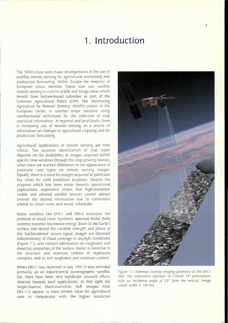
Radar satellites like ERS-1 and ERS-2 overcome theproblem of cloud cover. Synthetic Aperture Radar (SAR}systems transmit microwave energy down to the Earth'ssurface and record the variable strength and phase ofthe 'backscattered' return signal. Images are obtainedindependently of cloud coverage or daylight conditions(Figure 1.1), and contain information on roughness anddielectric properties of the surface. Radar is sensitive tothe structure and moisture content of vegetationcanopies, and to soil roughness and moisture content.

When ERS-1was launched in July 1991 it was intendedprimarily as an experimental oceanographic satellite,but there have been very significant research effortsdirected towards land applications. At first sight thesingle-channel black-and-white SAR images fromERS-1/2 appear to have limited value for agriculturaluses in comparison with the higher resolution

Figure 1.1. Sideways looking imaging geometry of the ERS-1SAR. The instrument operates at C-band, W polarisation,with an incidence angle of 23° from the vertical. Imageswath width is 100 km.

6

multispectral visible and infrared images from SPOTandLandsat. However, it is not difficult to become moreoptimistic once we see colour combinations of imagesacquired on different dates through the crop growingseason, particularly after image filtering techniques areapplied to reduce image speckle and improve definition.Further, when we take into account the fact thatERS-1/2 provide stable calibrated measurements ofsurface conditions which are unaffected by atmosphericeffects, one begins to appreciate some of the possibleadvantages over visible/infrared imaging.

This document (ESASP-1185)has been prepared by anESASpecialist Panel charged with the task of reviewingresearch work and progress so far, and makingrecommendations for future developments andintegration of satellite radar data into operational cropmonitoring systems. Chapter 2 of the documentprovides a general introduction to agricultural

information requirements and the potential role ofsatellite radar. Chapter 3 then develops anunderstanding of the information content of ERS/SARimages, concentrating on the presentation of resultsconcerning the temporal backscatter signatures ofagricultural crops. The different analysis techniquesbeing developed to extract agricultural information fromERS images are then presented in Chapter 4. Chapter 5contains case study results on temperate crops,including examples of the classification of arable crops,developments aimed specifically at early estimation ofcrop area, and combined analysis of ERS-1and opticalsatellite data. Case studies for tropical crops arepresented in Chapter 6, concentrating on developmentsfor rice mapping. Chapter 7 contains information oninteresting future developments in analysis techniques,and the potential of new multichannel satellite radarsystems. Finally,Chapter 8 provides overall conclusions,and recommendations for future developments andintegration into operational systems.

7

2. Agricultural Information and Remote Sensing

2.1. Application Objectives

Agricultural resources provide mankind with food andhave a substantial impact on the economic andenvironmental welfare of a particular country. The mainobjectives of the different parties interested in cropproduction, are the efficient and sustainable manage­ment and development of this renewable resource. AtEuropean and national levels, knowledge of changes incropping and crop production is the basic informationnecessary for the implementation of agricultural policy.The Common Agricultural Policy (CAP) involves acomplex arrangement of subsidies and tariffs used tocontrol European agricultural production. At the locallevel, decisions regarding crop types, varieties, plantingdates, irrigation procedures and fertilizers can benefitfurther from accurate knowledge of production on afield-by-field basis.

The monitoring of agricultural resources is time critical,and encompasses the following:• Crop condition assessment• Crop production forecasting• Mapping of crop area and monitoring changes• Surveillance of crop declarations for fraud control• Pollution detection and impact assessment (e.g.

erosion risk)

Traditionally, crop production forecasts have been basedon crop inventories and yield surveys. Crop inventoriesinvolve the identification of crops and measurement oftheir area. This can be achieved using census andground survey techniques. However, over very largeareas, the application of such techniques becomescostly and unreliable.

The use of satellite data to identify crops and measuretheir area has now revolutionised crop productionforecasting. In the early 1970's, the Large-Area CropInventory Experiment (LACIE)in the United Statesdeveloped the concept of an agricultural informationsystem incorporating satellite remote sensing. Multi­spectral satellite imagery are used to estimate crop area.Meteorological data from ground stations and NOAAsatellites are used to forecast yield and evaluate cropdevelopment stage.

2.2. The European MARS Programme

In 1988 the European Community initiated a ten yearresearch programme to build upon the US LACIEexperience. Monitoring Agriculture using RemoteSensing (MARS) is a major activity aimed at improvingEuropean production forecasts by the use of high­resolution remotely sensed imagery. Its main 'actions'include quantitative estimation of crop acreages in agiven region or country, vegetation and crop statemonitoring, timely crop yield forecasting of the meancrop yields per country, and the rapid and timelyestimation of the total production of the mostimportant crops within the EU. Its main users are theDirectorate General for Agriculture, and the EuropeanStatistical Office (Eurostat).

The first five-year project developed statistical methodsto estimate crop acreage and potential yield (calledMARS-STAT).The various activities of MARS-STAT,presented in Table 2.1, were conceived, developed andimplemented on the basis of inputs from approximately100 institutions from 17 European countries. Theseinstitutions provided data, models, algorithms andsoftware, after having previously validated them for useat the EU scale on the basis of country specificinformation.

Separate from the MARS-STATactivity, the use of remotesensing for verification and control of the area-basedsubsidies within the EU has evolved quickly over thelast few years and is now used operationally in mostcountries of the EU. This is known as MARS-PAC(Politique Agricole Commune), and involves the use ofcomputer-assisted photo-interpretation and automaticclassification to check farmer's applications forsubsidies. Approximately 5% of all farmers' returnswithin each country are now checked using satelliteremote sensing.

In general it can be said that both the LACIEand theMARS programmes were driven by economic motives,which, in a market driven by price, is easily understan­dable, and which can be seen as a very positive pointfor the long-term and intensive use of remote sensingdata. Taking this into account, as well as the fact that

the major interest in agriculture consists of obtaining asmuch timely information as possible on the crop area,condition and production, it can be seen that the use ofremote sensing can and will be extended to other

regions outside Europe within programmes similar toMARS-STAT.Major potential future customers couldcertainly be the Asian countries which have a require­ment to monitor rice resources.

8

2.3. Potential of Satellite Radar

All-weather acquisitionThe capability of satellite radar to provide reliable andfrequent imaging, independently of cloud coverage, is akey factor in the context of agricultural applications.Current European operational projects such as MARS­STATand MARS-PAC,are dependent on the acquisitionof multi-date optical satellite imagery acquired over themain crop growing season. Although the SPOTsatellitehas a variable viewing geometry which can be pro­grammed to increase the opportunities for imageacquisition, the ability to collect optical satelliteimagery within relatively narrow time windows can stillbe problematical in Northern Europe, where there are asmall number of cloud-free days. At least 17 of the 53current Action IV test sites lie above 50° North, withnew sites in Sweden and Finland being added in .1996.In the 1993 season, for example, only one or two SPOTor Landsat images were obtained for UK sites, whichhampered the provision of reliable crop determinations.The capabilities of ERS-1/2 are of even greaterimportance in tropical regions, where cloud cover ispersistent throughout the year.

High revisit frequencyThe ERS-1/2 satellites are able to acquire images for anylocation of the Earth's surface, at a repeat interval of atleast every 17 days, with the coverage frequencyincreasing in middle and high latitudes (Figure 2.1).Figure 2.2 provides an example of the data coverage ofof one of the MARS Action IV test sites; a total of 18images were acquired during the period 1 April to 31August 1993 for the Kings Lynn site in the UK.The all­weather day and night imaging capability guaranteesgood multitemporal coverage over the main growingseason.

Early data acquisitionClosely related to the cloud cover penetrationcapabilities is the potential of the ERSSARfor early cropidentification. Cloud cover and low light levels tend toparticularly hamper the acquisition of optical satelliteimages in the spring, and thus during the early part ofthe crop growing season. The use of radar for classifyingsoil surfaces being prepared for different crop types inthe autumn/winter period is a possible approach toearly crop identification.

Sensitivity to surface roughness and moistureThe ERS/SAR is sensitive to the geometrical character­istics of the ground surface, or the 'surface roughness',and the dielectric properties of the surface materials,

9

Figure 2.1.Coveragemap of ERS-1!SARfor the 35-day repeatcycle (nominal cycle of ERS-2)showing mid-image line andframe centres (dots).Descending orbits (day time passes)areshown in magenta, ascending orbits (night time passes) ingreen. At these latitudes, a frame (100x100km) has a largeoverlap with frames from adjacent passes, allowing morefrequent revisits for areas of interest.

lorbit frarte date trk8942 2547 9304Klt 2809092 1053 93<Mtt 4309214 2547 930-4.20 519321 1053 930'427 1589...43 2547 930506 2809593 1053 930516 4309715 25-47930525 St9822 1053 930601 15899-4"' 25-47 930610 2801009-41053 930620 43010216 2547 930629 5110a2a ross eacvceaset 0""45 2547 9307t 5 280tOSSS 1053 930725 43010717 254'7 9:30803 511002'41053930810158109"'6 25"'17930019 280t 1096 1053 930829 430

Figure 2.2. Typicalprint from the off-line catalogue user toolprovided by ERSUserServices,ESA!ESRIN,Frascati. It showsthe ERSframes covering an area of interest (shaded). Theframes are for the MARSsite Kings Lynn, UK.Between 1Apriland 31August1993, eighteen images were acquired, three ofthem during night time passes.

10

which are strongly correlated with moisture conditions.At the C-band wavelength of ERS there is very limitedpenetration through surface layers, and radarbackscatter of crops is determined by the structure ofcrop canopy (size, shapes and orientation of leaves,stems and seed heads), crop cover and moisturecontent. For soil surfaces, there is a strong sensitivity toboth the soil surface roughness and surface moisture(see detail in Chapter 3: Scientific Basis). The informationcontent of radar images is thus very different to that ofoptical satellite data, which record reflectance in visibleand infrared wavelengths.

Image geometryDue to the highly stable orbit of the ERS-1/2 satellites,images taken under the same orbital condition(ascending or descending), can be easily superimposedby a simple shift of the different images in relation tothe reference dataset. However, ERS SAR images aresubject to geometric terrain distortions related to thesideways looking imaging geometry (see Figure 1.1),which can impose some limitations on their use in hillyareas. In flat areas standard polynomial geometriccorrection techniques, can be used for geometriccorrection of ERSimages to levels of accuracy of about15 - 30 m. However, in hilly areas it is necessary to usea Digital Terrain Model (DTM)and specialised software toremove the geometric terrain distortions, in order toobtain accurate registration with topographic maps andcorrected optical images. Techniques for these types ofgeometric corrections are commercially available.

Complementary with optical and other radarsatellitesBesides the possibilities described above, there ispotential for improving crop identification, by takingadvantage of the complementary information providedby ERSand optical satellites. For instance, the use of ERSSAR data could concentrate on those crop types, forwhich SPOT or Landsat data do not provide clearseparability. Even with two to three dates of opticalimages, there can be problems in separating some croptypes which have similar visible near· and middle­infrared reflectance, and yet, these crop types may havevery different structural characteristics which are ableto be distinguished on ERS SAR images. The samepotential might become interesting when combiningERS SAR with the Japanese JERS or the CanadianRadarsat imagery. JERS operates at a different wave·length (Lband). Radarsat will acquire imagery withdifferent polarisation (HH) and incidence anglescompared to ERS-1.

There may be potential for using ERSSARdata, togetherwith agrometeorological backscatter models, to provideadditional quantitative estimates of crop growth. Thepotential for identifying soil moisture in ERSSARimagesmight equally become an important information inputfor future agricultural applications.

Products and costsThe present pricing policy and rapid delivery are bothimportant arguments for developing the use of ERS-1/2SAR for operational applications. ESA is developingvarious systems for rapid delivery of ERSdata products.The UK ERS-1 ground receiving station, for example,operates a facility for near real-time supply of ERS-1data using standard telephone lines. Latest informationabout ERSand available data products is available from:

ERS Help Desk at ESRIN:via Galiileo Galilei00044 Frascati, ItalyTel: + 39-6-941 80 600; Fax: + 39-6-941 80 510

II

3. Scientific Basis

3.1 Understanding Radar

The microwave radar carried by the ERS satellites hasthe potential to provide us with information onagricultural crops and the soil in which they grow. Aswell as generating images when visible/IR sensors areunavailable because of cloud, the information fromradars may be complementary to that from opticalsystems. The reason for this is the difference in theprocesses and scale sizes of features, with which radarand optical wavelengths interact in an agricultural field.The response of a field of crops to optical radiation isdetermined by structures on micron scales and byprocesses of chemical absorption. Microwave radiation,by contrast, penetrates significant distances into avegetation canopy and interacts most strongly withstructures (leaves, stems etc.) on scales comparablewith the radiation's wavelength (a few centimetres to afew tens of centimetres). Thus, microwave radars may

be thought of as probing in a very direct manner thestructural components of a plant canopy.

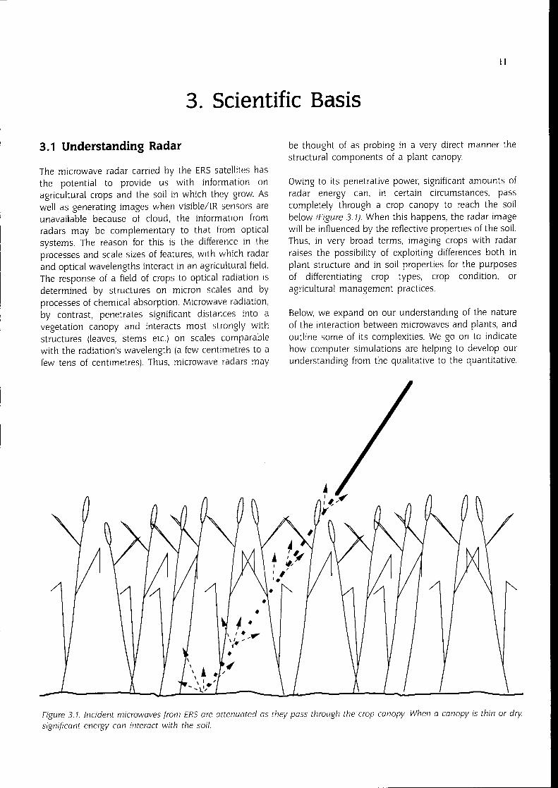
Owing to its penetrative power, significant amounts ofradar energy can, in certain circumstances, passcompletely through a crop canopy to reach the soilbelow (Figure 3.1). When this happens, the radar imagewill be influenced by the reflective properties of the soil.Thus, in very broad terms, imaging crops with radarraises the possibility of exploiting differences both inplant structure and in soil properties for the purposesof differentiating crop types, crop condition, oragricultural management practices.

Below, we expand on our understanding of the natureof the interaction between microwaves and plants, andoutline some of its complexities. We go on to indicatehow computer simulations are helping to develop ourunderstanding from the qualitative to the quantitative.

Figure 3. 1. Incident microwaves from ERS are attenuated as they pass through the crop canopy When a canopy is thin or dry,significant energy can interact with the soil.

12

The basis of interaction between radar andagricultural fieldsThe properties of vegetation and the soil whichinfluence the amount of microwave power scatteredback towards the ERSSAR fall under the two principalheadings of Geometric Structure and DielectricConstant. By structure we include the major plantconstituents on scales greater than a few millimetres(leaves, stems, flowers, fruits/seed heads). Their sizes,shapes and orientations determine the interaction ofindividual isolated components with the microwaves. Aflattened leaf, for example, scatters microwaves in adifferent directional pattern to a vertical stem. Below theplant canopy, the soil surface does not act as a simplemirror - rather the scattering from it is influenced byits roughness properties, especially on scales com·parable to the radar wavelength. The moisture of thesoil influences, through local chemistry, its dielectricconstant. For different soil types, there is a differentrelationship between moisture content and dielectricconstant, determined by the soil constituents.

The understanding of the interactions with individualplant components or the soil is relatively straight­forward. Electromagnetic modelling has at its disposala range of techniques and approximations to describethe scattering by at least the more simple shapes whichmay be encountered in a crop canopy or by a soilsurface with a known roughness profile. The realsituation, however, is rather more complex than that ofmicrowaves scattering off isolated plant structures orthe soil. The relative positions and spatial densities ofthe plant constituents determine how they respond asan ensemble to the radar, both through multiplescattering events or coherent interactions. Similarly, thesoil cannot always be considered separately from thecrop above it. Rather, a radar wave may be scattered bya leaf before being reflected off the ground and back tothe radar. Furthermore, the relative importance ofdifferent interactions, whether single or multiple (someinvolving reflecting off the ground and others not) isbelieved to change significantly as a crop developsduring the growing season (Figure 3.2).

Radar penetration and probing of crop canopiesDifferent wavelengths of microwaves have differentpowers of penetration into vegetation canopies -generally the longer the wavelength the greater thepenetration. The degree of penetration sets bounds tothe kinds of information which a radar can provide.Discrimination of crops based on their structures willonly be realised if the structures which differentiatethem occur within the volume probed by the radar. Thesame comment applies for the use of radars to probe

Wheat Backscatter Mechanisms

13

/

15

17I

.~·'..•..19

21I.··

23

25~~~~~~~~~~~~~~~~~~~~

Bare Soil Low Crop Full Crop Ripe Crop

Grow1h Stage

Figure 3.2. The changing contributions to the backscatteredradar intensity as a crop develops. Here, the example is afield of wheat where the crop cover is initially nil, thendevelops to a 10-cm deep canopy, followed in turn by a moistfull canopy and then a drier ripening canopy Initially, simplescattering off the soil dominates the total reflection. As thecrop increases in depth, the scattering from the soil becomesweaker, and is largely replaced by volume scattering withinthe canopy As the crop ripens and becomes moretransparent to ERS's microwaves, the soil becomes visibleonce again, and contributes to the total. together with morecomplicated scattering events involving radar waves interac­ting with both the canopy and the ground. (Source: R. Cordey,MRC).

soil characteristics; only if the radar can actuallypenetrate to the soil and back will there be any directinformation on soil moisture. The C-band radar of theERS satellites penetrates primarily only into the upperlayers of plant canopies when they are dense or moist.This penetration may increase very significantly,however, if the plant canopy becomes more transparentto radar as it dries out. Similarly, with the soil, the depthto which microwaves penetrate increases in drier soils.Thus, the influence of soil moisture on microwavebackscatter comes only from that moisture presentwithin the layer which is actually sensed.

Radar polarisation and incidence angleAs well as a radar's wavelength, the polarisation of themicrowaves and their angle of incidence relative tonadir, affects the interaction with plants and soils.Polarisation affects the way in which the microwavesrespond to different shapes and orientations ofscattering elements in a plant canopy. The vertically­polarised electric field of the ERS SAR interacts morestrongly with the vertical stalks of a field of grains thanwould, say, a horizontally-polarised radar. Such inter­action leads to differences both in the power scattered

back in those different polarisations and in the degreeof penetration through to the soil. Penetration to the soilis also influenced by the incidence angle of the micro­waves because that angle determines the path lengthwithin a crop canopy through which the radiation mustpass. A radar looking at a relatively steep angle, such asERS's 23 °, will tend to see the soil more readily than onelooking at a more oblique angle from nadir.

Towards a quantitative understandingDevelopments in the modelling of microwave scatteringfor agriculture have taken advantage of the increasingavailability of computing power, to create ever morerealistic and explicit models for the structures withwhich the radiation interacts. The models aim to explainor predict the brightnesses in radar images of differentcrop types under changing environmental conditions, ordifferent stages of growth during ~ season. Earlydevelopments in the 1970s were based aroundempirical or semi-empirical models for scattering atparticular wavelengths. These did not attempt torepresent crops as recognisable structures, but invokedtuneable parameters and were limited in theirapplicability over the wide range of radar and cropparameters which may be encountered. Widespreadrecent work has placed greater emphasis on realisticdescriptions of plant components, which can be relatedvery directly to measurable parameters (the shapes ofleaves, their thicknesses and moisture contents etc.). Itis conceivable that significant improvements in theaccuracy of predictions will entail even more explicitmodels of plants 'grown' in the computer, which includedescriptions of the spatial interrelationships betweenleaves, stems and fruits.

So how useful are computer models for understandingand predicting radar backscatter? A limitation on theiruse for quantitative predictions of image brightness isoften the lack of sufficiently detailed information on thecrop and soil itself. This has made experiments for thevalidation of computer models expensive and timeconsuming. Thus, models are probably of most currentuse in generating plausible radar images of agriculturalareas (e.g.for predicting the relative benefits of radars ofdifferent designs) or for investigating the likelysensitivity of image brightness to changes in crop or soilparameters. In that context, they support researchtowards methods for the retrieval of bulk crop or soilparameters (biomass, soil moisture for example),especially in the context of multi-date imaging whenonly a sub-set of possible parameters (e.g. moisture)may be changing rapidly.

13

Tosummarise then, it is widely believed that a relativelygood understanding has been developed of the inter­actions between microwaves and agricultural fields,which are responsible for the appearances of thosefields in a satellite radar image. Although complex, thewide range of interactions which microwaves mayundergo with plants and the soil - the sensitivity todetailed structure, moisture and chemistry - encourageus to believe that, given an appropriate set of radarmeasurements, it will be possible to discriminateeffectively between different crops. In the case of theERS radar, we will see that it is through its sensitivityto changes in crop structures through the growingseason that we have a tool for distinguishing differentcrops.

3.2 Calibration

What kind of calibration?For applications which demand more from a radarimage than just the detection or mapping of features,there is a requirement on the calibration of that radar.We need an understanding of how the radar imagebrightness relates to the fraction of incident microwaveenergy which a region reflects back towards the radarantenna. The accuracy with which a radar can becalibrated and the nature of that calibration influencethe range of information retrieval purposes to which theradar can be applied. By the nature of the calibration,we mean:• Has the radar been calibrated on an absolute

universal scale (relative ultimately to the signalreflected from a well-understood simple geometricalshape)? This sort of calibration is a pre-requisite forthe eventual retrieval of quantitative parameters ofcrops and soil from individual radar images.

• Is the radar calibration stable in time, albeit on apossibly arbitrary scale? Temporal stability ofcalibration permits us, in principal, to use multi-dateimages to quantify changes in crop and soilparameters.

• Is the radar calibration the same at differentlocations across a single image? Some degree ofstability in calibration across an image is needed inorder to create stable crop classification algorithms.

ERS-1 has been successfully calibrated over its entireperiod of operation against a scale defined by ground­based transponders. The units conventionally used arenormalised backscatter cross sections (sigma-zero, a0),

and are usually represented in their logarithmic decibel(dB) form. The dB value of sigma-zero is 10 log., of the

14

value in linear units. The intrinsic precision of thetransponders is believed to be better than 0.14 dB (i.e.an uncertainty of about 3% in the fraction of incidentenergy which they reflect). The long-term calibrationaccuracy of ERS-1relative to this scale is 0.06 dB withan rms error of 0.22 dB for a given image (Figure 3.3).Across an individual image (100 x 100 km 2), theestimated uncertainty in calibration is better than0.2 dB. Compared to previous experience with aircraftand satellite radars, these figures represent verysignificant improvements, and are achieved without arequirement for local calibration devices to be set out byan operational user. The method by which standard ERSimage products can be calibrated by the user isdescribed in the Appendix.

Limitations due to speckle noiseSynthetic-aperture radars suffer from a form of noise intheir images called speckle. Speckle is a consequence ofthe coherent nature of the SAR imaging process (it isclosely related to the phenomenon of laser speckle), andcan be a significant limitation on the measurability ofthe mean brightness from an area of land. The problemis that the brightness of a particular resolution cell,depends not just on some form of average of the plantand soil parameters in that area, but on the particularphase relationships between the reflected waves fromdifferent parts of that resolution cell. In the most basicof images, speckle typically imposes an uncertainty onthe estimate of the brightness from any resolution cellequal to the expected brightness. Only by some form ofincoherent averaging can a meaningful measurement ofimage brightness be made. Routinely, this is done inpart by a process known as multi-looking taking notone but two or more (3 in the case of standard ERSscenes) independent images and averaging together theradar brightnesses from each. Speckle can be furtherreduced by filtering the image, but at the expense offurther sacrificing spatial resolution. The purpose ofintroducing the concept of speckle here is to drawattention to the lack of requirement for very highcalibration accuracies for local scales of quantitativeanalysis. Figure 3.4 shows how, for ERS-1 imagery, theestimate of the mean brightness improves with the areaover which averaging is performed. For an individualfield of size 5 hectares, an ERSimage can provide at besta speckle-limited accuracy of 6% (or 0.27dB) for theaveraged brightness over that field. This is reasonablywell-matched to the stability of ERS-1 - a higheraccuracy of measurement would be unnecessary for theanalysis of fields of this size in individual images.

ERS-1SARStability

15

Otbll Number

05

13000

0 5

15

Figure 3.3. The stability of the ERS-1 radar is demonstratedhere by the apparent brightness in its images of one of theESA's transponders sited in Flevoland in The Netherlands.These transponders transmit back to ERS-1 a very precisefraction of the incident microwave energy and allow theradar's calibration to be checked independently. Followingthe application of the ERS-1 calibration procedure (seeAppendix), the brightness of a transponder is plotted for theentire duration of the 'Multidisciplinary Phase' of ERS-1operation from April 1992 to December 1993. (Source: R.Cordey, MRC).

-9Measurement Errors due to Speckle

(± 1 standard deviation)

-11

Field Area (Hectares)

Figure 3.4. ERS·1 intensity estimates as a function of integra­tion area. Due to speckle noise in SAR images, an individualpixel gives a poor estimate of a field's mean brightness. Ingeneral the more pixels that are average the better theestimate. The graph shows, for an actual ERS-1 standard 'PR!'image, how the mean brightness changes with the area ofimage which is averaged. The integration path is taken as aspiral out from a starting pixel, to mimic the averaging overfields of larger and larger sizes, up to a maximum area shownhere of 5 ha. For small integration areas, the uncertainty isclearly very significant, but the average settles down for fieldsof a few hectares to an uncertainty which is a small fractionof a dB. (Source: R. Cordey, MRC).

3.3 Temporal Signatures

The radar backscatter of a crop will vary over thegrowing season from early crop establishment throughto maturity and harvest. For the ERS radar, it is thesetemporal changes which may hold out the strongestprospect for establishing a routine means ofdistinguishing one crop from another. While we haveconfidence that the changes in radar backscatter of acrop during its development can be understood in termsof changes in the moisture and geometry of the crop orsoil, the problem facing potential operational users, is tobe sure that the profiles are sufficiently characteristic ofthe crop's development, and not of very localisedenvironmental conditions, to be of use in identifyingthat crop either regionally or globally.

For this reason, the nature of changes of backscatterwith time and the extent to which different crop typeshave distinctive temporal signatures, have been at the

-7

-8

-9

-10

-11

~ -12•..~ -13i.iu~ -14ui.ii:c

-15

-16

-17

-18

-19

31st May 1992

9th June 1992

15

focus of ERS-1 research studies undertaken in the UK,Germany and The Netherlands. In the followingsections, some of the principal results of these studiesare reviewed, with a view to identifying the extent towhich distinctive temporal signatures exist, and can beused as a tool for crop discrimination.

3.3.1 Cereal cropsA study carried out in the UK during the 1992 cropgrowing season, established that fields of winter wheathave temporal profiles in their ERS-1backscatter whichwere distinctive from other crops in the region (Woodinget al. 1993, Wright et al. 1993). The profiles showed aclear decline in early-season backscatter, followed by anincrease at the time of grain fill and ripening, and thena further major increase following harvest (Figure 3.5).

Repeating the study in 1993, revealed similar trends atfour sites across eastern England (Zmuda et al. 1994).Figure 3.6 shows the averaged temporal profiles at

Cultivation

13th September 1992

18th August 1992

14th July 1992

June SeptemberJuly August

Figure 3.5. Changes in winter wheat backscatter for a wheat field, development stages are also shown, Boxworth, UK, 1992.(Source: Wooding et al. 1993).

May

Figure 3.6. Mean ERS-1 backscatter temporal profiles for winter wheat, 1992 and 1993 growing seasons,for four sites in the UK. (Source: Zmuda et al. 1994).

16

(a) Bo IM'O rtho~~~~~~~~~~~~4~

•.....• ~~.....•-10.b -12

-14-16-18~o 1 , ii 1 , ii 1 , ii 1 , ii 1 , ii 1 , ii 1 , ii 1 , ii 1

100 120 140 160 180 200 220 240 260DayofYear

(c) Feltwell Peat

o~~~~~~~~~~~~~-~-4~~i -10~ -12

-14-16-18~o 1 , ii " ii 1 , ii 1 , ii 1 , ii 1 , 11 1 , ii 1 , 11 1

100 120 140 160 180 200 220 240 260Day of Year

these sites over the two years; as before, we see a setof declining responses in the early season followed byincreases through to harvest at around day 220. Despitethe overall broad consistency between sites andseasons, however, there are some notable differencesbetween the temporal profiles. The trough and inflexionpoints are possibly more marked in 1992, whilebackscatter is higher on day 167 in 1993 for Boxworthand the two Feltwell sites than would have beenexpected by the annual and inter-annual trends. Suchdeviations away from the overall trend can most likelybe explained as disturbances to the profile caused bymeteorological events (see § 3.4).

Q>) Teuingtono~~~~~~~~~~~~~~4~

i~'-'-10.b -12

-14-16-18~o '", 1 •• , 1, 11 1 •• , 1 ii, , , ii 1 ii, 1 ii, 1

100 120 140 160 180 200 220 240 260

19921993

DayofYear

(d) Feltwell Sand

0-.-~~~~~~~~~~~~~

~4~~

i-10~-12

-14-16-18~o 1 , ii 1 , ii 1 , •• 1 , 11 1 , ii 1 , 11 1 , ii 1 , 11 1

100 120 140 160 180 200 220 240 260

1993

Day of Year

But how do these profiles from UKwheat fields compareagainst those from elsewhere in Europe? In Figure 3.7,the UK trends are shown alongside profiles of winterwheat from the Dutch and German test sites. All thetemporal profiles do indeed show very similar patternsof change.

Changes in wheat backscatter with development stageGround data exist which give a clear visual impressionof the relationship between phases of the ERS-1backscatter curves and the development stages ofwheat crops. Figure 3.8 illustrates the crop developmentstages for one spring-sown and two winter-sown wheat

fields at Boxworth, UK, during 1993. These groundphotographs show the crop condition on four dates atthe time of ERS-1 SAR acquisitions, and may be used toprovide a more detailed interpretation of the processesresponsible for the changing response of the ERS-1radar:

On 19 April (day 109) the spring crop is only justemerging, in contrast with conditions in the winterwheat fields where tillering is well advanced and thereis over 90 % crop cover. Crop growth in the two winterwheat fields appears very similar, yet there is adifference of 1.7 dB in their backscatter. The backscatterof the spring wheat field is more than 2dB higher thanthe highest of the winter wheat fields.

By 24 May (day 144) the two winter wheat fields havewell developed flag leaves, and backscatter hasdecreased by 1.7 dB in the case of field no. 1.03, and3.5 dB in the case of field no. 1.05. Comparing the twofields, field no. 1.05 is seen to have a more verticalstructure than field no. 1.03 in which the flag leaves areseen to bend over. This structural difference seems to bea possible explanation of the difference in backscatterbetween the fields. In the spring wheat field, tillering hasreached a similar stage to that seen in the winter wheatfields on 19 April, and the backscatter has declined by3.5 dB to -12.14 dB, which is similar to the values ofthe winter wheat on 19 April.

On 28 June (day 179) all three crops were at the headingstage and appear quite similar in terms of structure,which is dominated by vertical components.Backscatter values for all fields reach a minimum at thistime (around -14 to - 16 dB), with only about 2 dBdifference between them.

Finally, on 2 August (day 214), grain fill and cropsenescence had occurred in all fields, and backscattervalues show increases of 1.5 - 2 dB for all fields. Inaddition to the obvious drying out of the crop by 2August, one can see that the senescence of the leafvegetation, with just the stalks and ears remaining, hasresulted in a less dense crop canopy.

The observed changes in winter wheat backscatter withcrop growth stage might be interpreted as follows. Atthe early stage of growth, as the crop emerges,backscatter is essentially determined by the conditionof bare soil, and in most cases backscatter values arerelatively high. As tillering takes place and crop coverdevelops, a decrease in backscatter is experienced, withvolume scattering within the crop reducing the overallreturn from the soil's surface. This reduction in

I7

0

-2-4

-6

-8ai"

-10:£·c -12

-14

-16

-18

-20100

- Gennany -9- UK --...- Holland

120 140 160 180 200 220 240 260Julian day

Figure 3.7. Comparison of winter wheat backscatter profilesfor the European test sites. (Source: M. Borgeaud, ESA/ESTEC,C. Schmullius, DLR and M. Wooding, RSAC).

backscatter seems to continue until flag leaves developand start to bend over and produce a more pronouncedhorizontal structural component to the crop. From thecomparison of different fields carried out above, it thenseems that a small increase in backscatter may actuallyoccur at this time, related perhaps to surfacebackscatter from the flag leaves. As heading takes placeand the flag .leaves become less dominant within thecanopy, the crop develops a more open verticalstructure which produces very low backscatter returnsfrom within the volume of the crop canopy. Then as thecrop begins to ripen, thin and dry out there is anincrease in backscatter which seems best explained byradar penetration through the crop to give somebackscatter contribution from interaction with the soilsurface.

Broadly, then, there is strong evidence to suggest thatwinter wheat backscatter shows consistent patterns ofchange as a function of time, namely that:• high backscatter is associated with the early stages

of crop development• backscatter then declines and reaches a minimum

by lune (ie the period of maximum crop productivity)• after anthesis backscatter increases during the grain

filling stage.

18

19/4/93

24/5/93

28/6/93

2/8/93

Field No. 1.04Spring Wheat

-8.65 dB

-12.14 dB

-14.01 dB

-l2.57dB

l.El Emergence[EJ Flag leaves emergedIQ] Grain fill

Field No. 1.03Winter Wheat

-10.98 dB

-l2.71dB

-13.77 dB

[I] TilleringIHl Heading

-12.47dB

Field No. 1.05Winter Wheat

-12.70 dB

-16.19 dB

-16.24 dB

Figure3.8. Changes in winter wheat backscatter with development stage, Boxworth, UK 1993, growing season.(Source: Zmuda et al. 1994)

Between-field variabilityFigure 3.9 shows individual temporal curves for wheatfields imaged by ERS-1 over the Netherlands test site.The profiles show similar trends in backscatterdevelopment as a function of time, but there is seen tobe a very significant variation in backscatter betweenfields on each date. This is much greater than can beaccounted for in terms of variations in the calibrationfactor across ERS-1 images. Accounting quantitativelyfor this variability has proved difficult. In the early

stages of development it may be most closelyassociated with differences in the percentage crop cover.Between-field variability in backscatter at the tilleringstage may perhaps be equated with variability in cropgrowth in different fields at any one time or with fieldorientation effects. Large variations in backscatter at theend of the season may be attributed to lodging (i.e.flattening of the crop by wind). Lodged fields have beenobserved to have higher backscatter than unlodgedfields (Wooding et al. 1993).

0Winter wheat

10 fields + average + stdev

-5

-100b

-15Average

+/- stdev

Mar Apr Moy JulJan Feb1993

Jun Aug Sep Oct Nov

Figure 3.9. Between-field variability in winter wheat backscatter, The Netherlands 1993.(Courtesy of M. Borgeaud, ESA/ESTEC)

Other cereal cropsThe UK,German and Dutch studies have also examinedbarley fields. Barley was seen to exhibit patterns ofchange similar to those of wheat with the notableexception that the backscatter minimum associatedwith the attainment of the heading stage occurs earlierthan for winter wheat. Figure 3. 10 shows comparisonsof wheat and barley signatures from the UKand Dutchtest sites. The period of maximum separation occursduring days 150 to 190. During this period wheat is atmaximum productivity (heading and anthesis) whilebarley crops are maturing (grain filling stage).Backscatter is at a minimum for wheat and is increasingas a function of time for barley. Therefore critical timewindows appear to exist during which different cerealcrops can be separated on the basis of their backscattertemporal signatures.

3.3.2 Other arable cropsA composite of temporal profiles for a mixture of arablecrops studied with ERS·1 at the German, Dutch and UKtest site is shown in Figure 3.11. The curves illustrateclearly the varying potential for inter-crop discrirnina­tion which ERS-1may provide as a function of time inthe growing season. Below, we pick out certain im­portant crops and summarise briefly their backscattercharacteristics and their perceived potential foridentification.

Sugar beetTemporal profiles of sugar beet (Figure 3. 12) tend not toshow the large changes through the season which arecharacteristic of cereals. Rather, it appears that aftercanopy closure, backscatter remains at a uniformly highlevel. Variations in backscatter between different fields

19

20

ca)Hollm:i

-4--- W. Batley '93

Julian Day

Winter Wheat

UK (109J)

D (1192)

5 121126J 101724l17 1421285 1211282 ' 162J30f5 132027•••• ..., ••••• ..,., ""9""' -,..,

-e- W.Wheat '93

(b) UK-Felt'tlell Se.nd0.....-~~~~~~~~~~~~~~~~~---.

-2-4-6-8

~ -10\> -12

-14-16-18-20 I •ii 'I II II I' ii I I I ii I j 11 I I Iii II I' ii I I' II I I ii II Iii I I Iii ii II II I I ii II I

0 20 40 60 80 100 120 140 160 180 200 220 240 260Julian Day

o~~~~~~~~~~~~~~~~~~~~~-2-4-6-8

~ -10.b -12

-14-16-18-20 1ii ii I' ii 1I' 1 1 1 j 11 1 1I' 1 ii I' 1 1 1I' 1 ii I1 1 ii I' 1 1 1 j ii 1 1 j ii ii j 1 1 1 1 i' 1 1 1 j

0 20 40 60 80 100 120 140 160 180 200 220 240 260

Figure 3.10. Changes in mean winter barley and wheat backscatter as a function of time (a) 1993 growing season, TheNetherlands (Courtesy of M. Borgeaud, ESA/ESTEC);(b) 1993 growing season, Feltwell, UK. (Source:Zmuda et al. 1994).

Sugarbeet Potatoes

-·

-10

-s

-10

-201 I I I I 11 I I I I I I I !I I I I I I I I I II I I I !I5 1211263 101724317 1421285 1211262 I 1823306 132027

Aprl Moy ..1111\e Juty Ar.19u•t S.ptem~r,..,Gro•ln~ seo.on 1993

Figure 3.11. Changes in wheat, sugar beet and potato backscatter with time for the European test sites.(Source:M. Borgeaud, ESA/ESTEC,C. Schmullius, DLR and M. Wooding, RSAC).

0Sugorbeet

10 fields + overage + stdev

-5

-10Db

-15Average

+/- stdev

Mor Apr Moy AugJon Feb1993

Jun Sep NovOctJul

Figure 3.12. Between-field variability in sugarbeet backscatter, Flevoland, The Netherlands 1993.(Source: M. Borgeaud, ESA/ESTEC).

is greatest during the early part of the season at somesites while others show greater consistency; possiblyreflecting differences in management practices in thedifferent countries. In particular, sites in the Netherlandshave exhibited a deep dip in backscatter before theemergence of the crop.

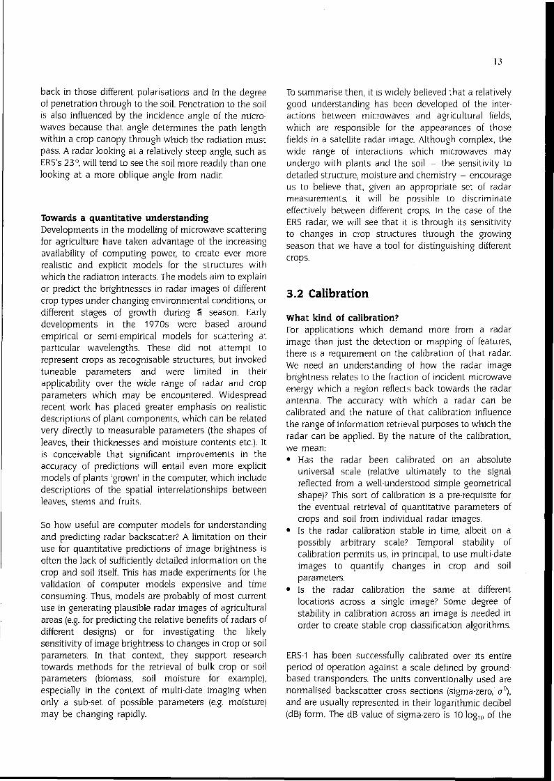
Oilseed rapeOilseed rape does show significant features in itstemporal profiles although, again, not nearly aspronounced as for cereals (Figure 3.13). During and afteranthesis (May and June), backscatter increases followedby a decline during senescence and seed ripening untilharvest in mid August. The backscatter of the roughbare soil after harvest may be several dB brighter thanpre-harvest levels. Compared to winter wheat, oilseedrape profiles display higher backscatter at all stages ofdevelopment up to late July. Maximum backscatter forrape seed occurs at the seed development stage in June.At this time winter wheat backscatter is at a minimum.Following ploughing at the end of the growing season,similarly high backscatter values are associated withrough bare soil fields which had previously held eitherrape or wheat.

PotatoesPotatoes, and indeed other root crops which have beeninvestigated, tend to show less variations in backscatter

through the season than either winter sown cereals oroilseed rape. Some differences between different sitesare seen, especially in terms of the variation inbackscatter about the mean. Scatter is greatest duringthe early part of the season which may be attributableto differences in the height and orientation of soil ridges,and to variability in above ground vegetation cover indifferent fields.

3.3.3 RiceERS-1radar backscatter from rice fields exhibits a verycharacteristic and pronounced temporal signatureduring the growing season. This is associated with verysignificant changes in the nature of the crop, and of thegrowing medium during each growth cycle, which aremore dramatic than those previously described fortemperate arable crops.

Rice fields are flooded during the early growing stagewith the soil surface almost completely covered bywater. Plants emerge above the water surface, andincrease in height up to a maximum level after whichthe ripening phase starts. Plant moisture content is highat the early growing stage, and drastically decreasesduring ripening. In most cases water is drained out fromthe field at the beginning of the ripening phase, leavingthe soil surface moist. Before harvest the soil becomesdrier and rougher due to cracks in the surface. It is these

21

22

-5

-6 5th July 1992

-7

31st May 1992

-9

-10

May June

13th September 1992

SeedRipening

14th July 1992

··,)'.

July August September

Figure 3.13. Changes in oilseed rape backscatter with time, development stages also shown, UK 1992.(Source: Wooding et al. 1993).

structural and moisture changes which are believed tobe the main cause of changes in the nature of the radarinteraction and consequently of the ERS imagebrightness.

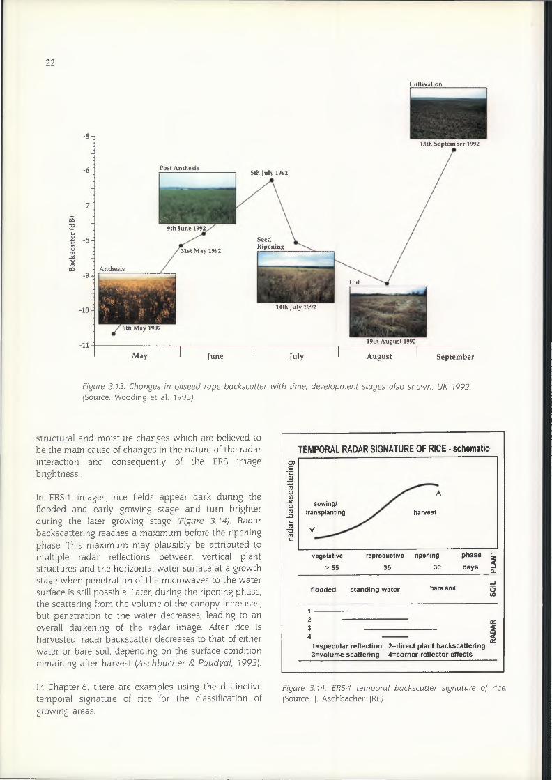
In ERS-1 images, rice fields appear dark during theflooded and early growing stage and turn brighterduring the later growing stage (Figure 3.14). Radarbackscattering reaches a maximum before the ripeningphase. This maximum may plausibly be attributed tomultiple radar reflections between vertical plantstructures and the horizontal water surface at a growthstage when penetration of the microwaves to the watersurface is still possible. Later, during the ripening phase,the scattering from the volume of the canopy increases,but penetration to the water decreases, leading to anoverall darkening of the radar image. After rice isharvested, radar backscatter decreases to that of eitherwater or bare soil, depending on the surface conditionremaining after harvest (Aschbacher & Paudyal, 1993).

In Chapter 6, there are examples using the distinctivetemporal signature of rice for the classification ofgrowing areas.

TEMPORAL RADAR SIGNATURE OF RICE - schematic-enc

~(,JI/).li:(,Jns.c•...ns't:J~

sowing/transplanting harvest

vegetative reproductive ripening

> 55 35 30

phase I-zdays 5~

-I0I/)

flooded standing water baresoil

1----234

0::c(0

~1=specular reflection 2=direct plant backscattering3=volume scattering 4=comer-reflector effects

Figure 3.14. ERS-1temporal backscatter signature of rice.(Source: j. Aschbacher, jRC).

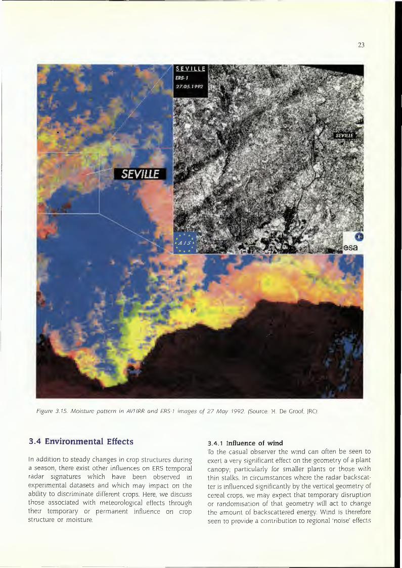
Figure 3.15. Moisture pattern in AVHRR and ERS-1 images of 27 May 1992. (Source: H. De Groof, )RC).

3.4 Environmental Effects 3.4.1 Influence of windTo the casual observer the wind can often be seen toexert a very significant effect on the geometry of a plantcanopy; particularly for smaller plants or those withthin stalks. In circumstances where the radar backscat­ter is influenced significantly by the vertical geometry ofcereal crops, we may expect that temporary disruptionor randomisation of that geometry will act to changethe amount of backscattered energy. Wind is thereforeseen to provide a contribution to regional 'noise' effects

In addition to steady changes in crop structures duringa season, there exist other influences on ERS temporalradar signatures which have been observed inexperimental datasets and which may impact on theability to discriminate different crops. Here, we discussthose associated with meteorological effects throughtheir temporary or permanent influence on cropstructure or moisture.

23

24

on the temporal backscatter signatures of crops. Asidentified in temporal signatures of wheat in § 3.3.1,extreme wind disruption of the canopy late in theseason (i.e. crop flattening or 'lodging') does lead tosignificant and irrecoverable changes in backscatterlevels, leading to populations of outliers in distributionsof crop signatures.

In the case of rice, the wind also influences the surfaceconditions; in this case the water surface present for atleast part of the growing cycle. Wind during the earlygrowing stage increases the roughness of the watersurface, resulting in enhanced radar backscattering.Such effects are, indeed, seen in ERS-1 imagery of ricefields, and an example will be presented as part of thecase study of Chapter 6.

3.4.2 The effect of rainfall eventsERS images are potentially sensitive to moisture, bothwithin crops and, under some circumstances, within theupper layers of the soil. Rainfall, therefore, mayconstitute an additional 'noise' source affectingtemporal radar profiles otherwise related to cropdevelopment. Significant enhancements to ERS-1imagebrightness are, indeed, seen to be associated withrainfall events over agricultural areas. Evidence comesfrom a small subset of temporal radar profiles, includingsome of those obtained in 1993 from the UKtest sites.Figure 3. 15 provides an illustration of rainfall effects onradar backscatter across an ERS-1 scene of the Sevillearea. In this example alternate light and dark zoning isseen in a part of the image where the similarly timedAVHRRimage shows the presence of rain bearing cloudformations. In quantitative terms, rain events in the UKwere observed to result in enhanced backscatter onparticular days of up to 4 dB (i.e.a factor of 2.5 increasein reflected energy).

The effect of rainfall may have a significant effect on thecomparison of radar observations both betweendifferent sites and different seasons. As a result, cropclassifications to the highest potential accuraciesachievable with ERSor other future satellite radars mayneed to be based primarily on local training ofalgorithms. However, with a sufficient number ofmeasurements over a number of seasons, it may bepossible to isolate accurate meaningful profilescharacteristic solely of crop development.

4. Analysis Techniques

4. 1 Pixel-based Approach

Computer-based crop classification using radar imageryis complicated by image speckle, which is a noisephenomenon of the radar imaging process (see § 3.3).There is a linear increase of noise level (expressed as thestandard deviation of pixel values within a uniformland-cover area) with the average grey value.

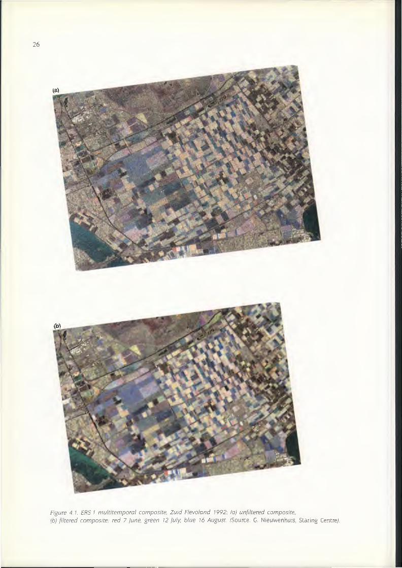
Image speckle hampers the application of standardpixel-based classification techniques normally used toclassify optical imagery. If one adopts a pixel-basedapproach it is first necessary to apply some form ofimage filtering or segmentation to reduce image specklebefore image classification. Figure 4. 1 illustrates theeffect of the Gamma-Gamma MAP filter (Lopes et al.,1993) applied on a multi-temporal ERS-1 composite ofZuid Flevoland in the Netherlands. Both unfiltered andfiltered images are shown, and one can see how thewithin field variability has been reduced considerably inthe filtered image, while edges of linear features havebeen preserved. Speckle reduction filters aim to reducespeckle while preserving spatial resolution and linearfeatures.

Paudyal & Aschbacher (1993 a.b} have systematicallyinvestigated the performance of different filters, using astudy area in Thailand. The speckle-specific filters testedincluded the Lee Local Statistics, Lee Sigma, Frost, Li,

MAP and Gamma MAP filters (Lee, 1986.; Frost et al.1982.; Li, 1988.; Nezry et al., 1991). The investigationincluded a number of non-speckle-specific filters, suchas mean and median filters.

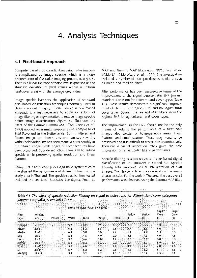
Filter performance has been assessed in terms of theimprovement of the signal-to-noise ratio SNR (mean/standard deviation) for different land cover types (Table4.1). These results demonstrate a significant improve­ment of SNR for both agricultural and non-agriculturalcover types. Overall, the Lee and MAP filters show thehighest SNR for agricultural land cover types.

The improvement in the SNR should not be the onlymeans of judging the performance of a filter. SARimages also consist of heterogeneous areas, linearfeatures and small scatters. These may need to bepreserved and it is difficult to assess this quantitatively.Therefore a visual inspection often gives the bestimpression on a particular filter's performance.

Speckle filtering is a pre-requisite if pixel-based digitalclassification of SAR imagery is carried out. Specklefiltering also improves visual interpretation of SARimages. The choice of filter may depend on the imagecharacteristics. For the work in Thailand, the best overallperformance was observed using the Gamma MAP filter,

25

26

Figure 4.1. ERS-1 multitemporal composite, Zuid Flevoland 1992; (a) unfiltered composite,(b) filtered composite: red 7 June, green 12 July, blue 16 August. (Source:G. Nieuwenhuis, Staring Centre).

which was found to give the best combination ofsmoothing image speckle within homogeneous areasand edge preservation. Application of the Gamma MAPfilter also improved visual interpretation. The Lee filterperformed well for digital analysis when classseparation was critical. However, edges and linearfeatures tended to be degraded.

The application of speckle filters in the Thailandagricultural study areas has shown that land coverdiscrimination can be significantly improved.Classification performance also shows improvement.This is further developed in Chapter 6.

4.2 Field-based Approach

A field-based approach involving the use of digital fieldboundaries to extract image statistics, such as themean field backscatter, effectively overcomes theproblem of speckle. Clearly such an approach assumesthat fields can be treated as individual objects and onecan disregard the within field spatial variability. Ingeneral, only the mean field values are used forclassification, but within-field variance and texture canbe used as additional information for crop classification.At the spatial resolution of satellite radar, agriculturalfields are relatively smooth uniform surfaces, lackingthe grainy texture which can be associated with urbanor forest areas.

An example of a field-based classification methodologyusing ERS-1 images integrated with digital fieldboundaries derived from a SPOTXS image is presentedas a flow chart in Figure 4.2. In this example, digital fieldboundary information is stored in a GIS.A selection ofERS-1 acquisition dates is made, and the meanbackscatter value (gamma) per field is calculated usingthe digitized field boundaries. These mean values areused to create signatures for each crop type, and tocarry out a maximum-likelihood classification. Theclassification result is then added to the GISto producea land cover map.

Field boundaries can be obtained from cadastral maps,and then adjusted over an image backdrop, oralternatively can be obtained directly from radar oroptical satellite images using visual interpretation orautomated techniques.

When only ERS images are used to extract field boun­daries, multitemporal composites aid the interpretationof field boundaries. Figure 4.3a shows field boundariesmapped over a multitemporal ERS-1image of Terrington

27

Spot· XS ERS-1 SAR pu

Lot boundaries Visual1nterpre1a1ion

andon-screend1911111ng

Tra1nmgdata Field-basedc!assilicauon

Crop type

Figure 4.2. Flow chart of a field-based classification proce­dure of ERS-1images using additional information from topo­graphical maps, field work and optical data.(Source: Schotten et al. 1994).

(a) ~~J:-1M~~~-~~~~~~~9~ackscatterCompositeGreen: 16thMay1993Blue: 11thAprll 1993

(b) ~~J,"1M~~~:~~~eB1a9c:3scatterCompositeGreen: 16thMay1993Blue: 11thApril 1993

Figure 4.3. ERS-1 multitempora/ backscatter composites,Terrington Marsh UK; (a) PR! imagery (b) mean fieldbackscatter composite. Field boundaries are superimposed.(Source: M. Wooding, RSAC).

Marsh in the UK.The speckle effects are very evident inthe backscatter composite as fields appear to contain

28

noise. A GIShas been used to capture field boundarieson screen using ERS-1 imagery as a 'backdrop'. As theERS-1imagery is georeferenced to the UKnational grid,field boundaries can be linked to the radar image.However, edge effects have to be removed and this isachieved by creating a buffer zone around theboundaries. Field means can then be extracted andstored in the database of the GIS.Mean field backscattercolour composites can be produced by seed filling thefields with the mean values, as shown in Figure 4.3b.

Optical satellite images usually provide a betterdefinition of linear features, and can be used as thesource of field boundaries to be used for field-basedanalysis of satellite radar images. Harms et al. (1993)have performed an automated segmentation of a SPOTimage as a basis for classifying multi-date ERS-1imagery. The technique produced classificationaccuracies very close to those achieved by visualinterpretation of field boundaries on optical images.Following georeferencing of the SPOTand ERS-1imagery,segmentation of the SPOTimage was performed usingthe principal of local contrasts. The segmentationperformed over a large variety of agricultural crops hasindicated the high quality and robustness of thealgorithm. Comparisons with cadastral maps show over95 % accuracy for the segmentation. Having segmentedthe optical dataset, multitemporal ERS images wereclassified by a field-based algorithm using mean andstandard deviation. The results obtained using thisanalysis process are shown in Figure 4.4.

A number of automated segmentation techniques arenow being developed to identify parcel boundaries, andundertake field-based classification, directly using radarimages. Techniques developed by White (1994) andQuegan et al. (1993) involve operations such as mergingof an initial 'fine segmentation' based on calculatedprobability, edge detection and region growing, and theestimation of background radar cross section. Resultsobtained within different studies show the usefulness ofsuch algorithms for segmenting imagery and classifyingcrops. Example images are shown in Figure 4.5.

4.3 Integration of Optical and Radar Data

One example of the integrated use of optical and radardata has been presented in the previous section, wherea SPOT image has been used as the source of fieldboundaries for subsequent multi-temporal classificationof ERS-1 images. Improving crop classification bycombined analysis of the reflectance and backscatter

data, respectively from optical and radar images, takesthis one step further.

As yet, techniques for fully integrated analysis of opticaland radar data are poorly developed. However, as far asvisualisation of combined data sets are concerned,some interesting results have been obtained using the!HS technique (i.e. Intensity-Hue-Saturation). Normally,colour composites are produced using the red (R),green(G)and blue (B)colour guns to display different spectralor temporal channels. However an alternate colourspace can be defined which uses Intensity, Hue andSaturation:• Intensity is the overall brightness of a scene• Saturation represents the purity of colour• Hue represents the colour or dominant wavelength

of the pixel.

The intensity, hue and saturation components can alsobe displayed as a colour composite or they can becontrast stretched before being transformed back intoRGBspace. One of the main advantage of the techniqueis that it enables the information content of more than3 channels to be visualised. The steps involved incombining optical and radar imagery using thistechnique are as follows:1. register SAR and optical images,2. convert a 3-band optical image from RGB to !HS

coordinates,3. substitute the SARimage for the intensity coordinate,

and4. convert back to RGBspace.

Figure 4.6 provides an example of this data integrationtechnique, using Landsat TM and ERS-1images for anarea in Johar State, Malaysia. The resulting colourcomposite seems to provide enhanced discrimination ofland cover types in comparison with what is possibleusing either just the Landsat or ERS-1data. However,note that the mountains in the top of the compositecontain terrain distortion from the ERS-1image.

4.4 SAR Interferometry

A promising new technique is being developed usingSAR interferometry. Interferometric processing of SARdata combines complex valued images for two passesto derive precise measurements of the difference in pathlengths for the two sensor positions. Either airborne orspaceborne SARcan be used to create interferograms.ERS-1operated during several phases with repeat orbitsof 3 and 35 days. These repeat orbits are useful forperforming SARinterferometry. Thanks to the excellent

Figure 4.4. Field-based classification procedure by combining optical with ERS-1 imagery(a) SPOT image of July 1992(b) Segmentation of SPOT image based on ARKEMIE software(c) ERS-1 multitemporal composite (red: May; green: July; blue: August;td) Segmentation based per field classification of multitemporal ERS-1 imagery;classification results: yellow = rice, white = other crops, brown = misclassified.(Courtesy of 1. Harms, Scot Conseil).

(a)

(c)

29

(d)

Figure 4.5. Multitemporal ERS-1SARcomposite of Feltwell UK. (a)before speckle reduction; (b)after speckle reduction using edgedetection and region growing; red: 11 April 93, green: 20 June93, blue: 29 August 93; (c) parcel boundaries derived fromsegmentation. (Courtesy of the Centre for Earth Observation, University of Sheffield, UK).

30

(a)

(c)

orbit and attitude control and the reliability of the SARsystem, interferograms may be produced. Mainly as aresult of high quality ERS-1 SAR data and extensivecoverage, the development and application of repeat­pass SARinterferometry has become one of the primeresearch activities within the radar remote sensingcommunity. The primary SAR interferometry applica­tions are the preparation of height and differentialdisplacement maps.

Figure4.6 /HScombination of Landsat TMand ERS-1images,Johar.Malaysia. (Source:M. Wooding, RSACJ.

A significant amount of research is being undertaken tofurther refine the image processing steps required forthe estimation of the interferometric phase, with thegoal of an optimization of interferometrically derivedheight (Zebker et al. 1994) and displacement maps(Massanet et al. 1993). However, it has been shownrecently that SAR interferometry has also a largepotential for forest and agricultural applications (Askne& Hagberg 1993, Werner & Wegmiiller 1994, Wegmiilleret al. 1995a), particularly in providing a means forseparating agricultural fields from forests in SARimages ..

Using SAR interferometry, forest mapping with ERS-1becomes almost straightforward (Wegmilller et al.1995b). The interferometric correlation observed overforest is low due to the dominance of volume scattering

and the geometric changes occurring between therepeat pass data acquisitions. The low interferometriccorrelation of forest can easily be distinguished from themuch higher correlation shown by low vegetationcanopies and bare soil surfaces.

In Figure 4.7, differences in land cover classes areshown by displaying the interferometric correlation, thebackscatter intensity from one of the passes and thebackscatter intensity change as a colour composite.This SAR interferogram was derived using ERS-1 SLCdata measured on 24 and 27 November 1991. Theregion shown covers agricultural, urban, and forestedareas, as well as a number of lakes near Bern in centralSwitzerland. The image covers an area of approximately45x45 km.

31

Figure 4.7. Interferometric signatures derived from an ERS-1SAR image pair over Bern, Switzerland (red: interferometriccorrelation; green: backscatter intensity on 24 Nov.; blue: backscatter intensity change between 24 and 27 November). Water(blue), forest (green),sparse vegetation (orange/yellow), and urban areas (yellow/green), as well as certain farming activities(green/blue) and frost (magenta) can be identified. (Source: RSL, Zurich, Switzerland).

33

5. Temperate Crops

5. 1 Classification of Arable Crops

UK exampleExamination of backscatter time series (§ 3.3, UKsites)reveals that there are critical periods or windows in thecrop calendar, in which certain crops can be separatedon the basis of their backscatter profiles. By selectingdifferent date images and combining them as colourcomposites, one is able to show this discrimination overan agricultural area. Research studies carried out in theUKhave shown that images acquired from late May tolate July can be used to discriminate wheat, barley,oilseed rape, sugar beet and grass.

Figure 5.1 shows a multi-date colour composite of ERS-1images acquired in late May and June 1993. This colourcombination has been chosen to highlight discrimina­tion of winter wheat and oilseed rape. In this composite,winter wheat fields have the darkest signatures incontrast to oilseed rape fields which have the brightestsignatures. This is because wheat backscatter is at aminimum, and rape backscatter is at a maximum for allthree dates (compare also the temporal profiles in§ 3.3).Two large winter barley fields in the top right hand ofthe composite have purple signatures, others showsome purple colour. This is because winter barleybackscatter has increased on the 13 and 29 Junerelative to wheat fields, which have low backscatter onall three dates. Other crops exhibit similar signatures atthis time, because these fields contain bare soilundergoing management operations for the establish­ment of root crops (sugar beet and potatoes) and peas.Colour composites such as that described reveal thatacross the UK test sites:• winter wheat has the darkest signatures because of

low backscatter during this time period, and can beeasily discriminated from all other crops;

• oil seed rape has the brightest signatures associatedwith very high backscatter in this period, and istherefore well discriminated from all other agricul­tural crops;

• winter and spring barley have purple signaturesassociated with increases in backscatter due torelatively early crop senescence;

• root crops have different colour signatures comparedto rape and cereals, which is associated with baresoil conditions early in the crop growing season.

In the UK study, backscatter response for fields isrepresented by the field averages calculated byintegration with digital field boundary information heldin a GIS.Therefore the use of mean field backscatter forcrop classification is investigated. Using meanbackscatter on · critical dates and differences inbackscatter between dates, threshold values areexplored as a way of classifying crops usingdiscriminant analysis within the GIS database.

The 1993 UK database includes the croppinginformation for a total of 783 fields spread across 4 testsites. This dataset was divided into two, after assigninga random number to each field and sorting thedatabase on that number. Backscatter differences weretaken from 11 April to 29 June, and from 29 June to 3August. One half of the dataset was used to generatetraining statistics for thresholds. The rest of the datawere used to test the thresholds for crop classification.

Patterns of change were found to be unique for oilseedrape, compared to other agricultural crops. TheApril/June backscatter difference shows a negativechange compared to other crops, whilst the June/Augustdifference is positive. This was used to threshold fieldsnot included in the training set. A threshold forbackscatter on a single date (13 June) was also includedin the classification. Oilseed rape fields can bediscriminated with 100 % accuracy using such aclassification strategy.

The use of the methodology for classifying winter wheatwas then investigated. Again, backscatter differencesand single date backscatter thresholds were applied tothe data not included in the training data. Thebackscatter difference thresholds were obtained fromthe training set. It was found that very high orders ofclassification accuracy could be obtained by usingbackscatter on two dates instead of one. The two datescorresponded with the period of minimum wheatbackscatter (late May and late June). Table 5.1 shows thebreakdown in classification performance by test site,with accuracy being at least 90 % in all three cases. Thischange detection thresholding approach is seen to haveconsiderable potential for classifying crops using multi­temporal ERS-1SARdata.

34

Table 5. 1 Classification accuracy assessment for wheat by site, UK (Source: Zmuda et al. 1994)

Figure 5.1. ERS·1multitemporal composite, Boxworth UK (red: 25 May; green: 13June,blue: 29 June 1993).Field boundaries andcropping are superimposed. W wheat; R: oilseed rape; L: linseed; G:grass. (Source: Zmuda et al. 1994).

Total No.No. Classified % CorrectSite

BoxworthTerrington

4041

9597.5

3840

Feltwell 69 9061

Omission Fields CommissionedCommission

2 72

grass (7)linseed (1)potatoes (1)grass (2)oats (1)spring barley (1)

Classifications for winter barley using the thresholdapproach have been attempted. However, initial resultsindicate that barley is confused with other crops.Therefore the use of multivariate statistical analysis maybe more appropriate for separating the cereals. The useof backscatter profile models and first and second orderturning moments is under investigation for the UKdata.

German examplesThree ERS·1 SAR images have been used together with

8 4

airborne E·SARimages of the Lechfeld testsite, located70 km west of Munich, Schmullius et al. (1994). Figure5.2 is a multitemporal colour composite of the threeERS·1 images acquired in June and July 1992. Thecolours indicate the radar backscatter variations over

".time. The brightest fields on the multitemporal imageare sugar beet fields. This crop had the highestbackscatter throughout the six-week period. Thedarkest fields are cereals. Colour variations areindicative of crops undergoing significant changes inbackscatter between 1 June and 6 July.

Table 5.2 Confusion matrix (percent of training site pixels) in percent. Lechfeld testsite, Germany(Source: C. Schmullius, DLR)

Class Fallow S. Barley W. Barley W. Wheat Sugar beet Oilseed Rape

Fallow 40.1 1.1 16.1 0 37.9 4.8S. Barley 0.4 75.5 5.4 14.6 1.4 2.5W. Barley 0 27.6 58.6 0 7.3 6.9W. Wheat 1.1 56 3.5 32.2 2.4 4.8Sugar beet 8.9 1.2 9.2 0 66 14.7Oilseed R. 1.9 1 0 0 25.3 71.7

Figure 5.2. ERS-1multitemporal composite, Lechfeld Germany,1992 (red: 1 June, green: 20 June, blue: 6 July).(Source: C. Schmullius, DLR).

The use of a Maximum Likelihood Classifier wasinvestigated. Figure 5.3 shows the resultingclassification for six crop classes (winter wheat, summerbarley, winter barley, sugar beet, oilseed rape andfallow). The confusion matrix of the training site pixelswhich were correctly classified, was calculated after a5 x 5 median filter and a sieving window were applied

351 •

LEGEND:Winter Wheat~~·~~~ -..irley

l9ySugar BeetOilseed RapeFallow

Figure 5.3. Pixel-based ERS-1 maximum likelihood classifica­tion of Lechfeld, Germany (Source: C. Schmullius, DLR).

to the classified image to reduce the effect of speckle. Inthis case the average (unweighted) overall classificationaccuracy is only 57 % . However, there is little doubt thatthis could be improved significantly by better choice ofimaging dates and by using segmentation techniques.

Table 5.2 illustrates the misclassification (due tostatistical ambiguity of the covariance matrix) betweenfallow, sugar beet, cereals and oilseed rape. Theseresults from the German test site are in accord with theUKfindings presented above; in that cereals are easilydiscriminated from high biomass crops such as oilseedrape and sugar beet, as shown here. A better separationof grain crops or between rape and sugar beet might bepossible with more multitemporal information. For largearea applications, such as mesoscale climate models, a

36

mere separation into only three classes (cereal, large leafcanopies and fallow/grassland) could be feasible interms of biomass estimation for evaporationcalculations. In this case, a 3-class confusion tablewould show the following values along its diagonal:fallow 40 % , cereals, 91% , and large leaf canopies 83 % .The average accuracy then reaches 71% .

Dutch exampleERS-1SARimages acquired from the beginning of Mayuntil the end of October 1992 have been used to mapagricultural crops for the Flevoland test site in TheNetherlands. Figure 5.4a is a multitemporal colourcomposite of the test site with field boundaries derivedfrom a SPOTmultispectral image. Figure 5.4b shows theground reference data for each field, and Figures 5.4c &d the crop classification results, obtained using pixel­based and field-based approaches, respectively. A visual

Figure 5-4. ERS-1SARimagery and crop classification resultsusing field-based and pixel-based approaches, Zuid Flevo­land, 1992. Source: G. Nieuwenhuis, Staring Centre.(a)ERS-1multitemporal colour composite (red: 7 June,green:12 July, blue: 16 August).

UID FLEVOLA:1[rtdt"IP.nu~ dote llJ9'"'

.pqtQ\oM•~11111.11 t••I\.I -~u.r'*11•\I(•\irQlll'I ilhl,l>l'f•wlf\Wr rol)t

~p!Ml\IIXlrlW)'

I011Jn.1lll•O/llO"V•.......·~Q·11,r.1:'"1011Ul'f,'fllJhi.111 llul.11

(b) Referencedata

inspection of these classification results in conjuctionwith the ground data map shows that crops likegrassland and winter wheat are accurately classified,but the sugar beets are mixed with the potato crop.

Schotten et al. (1995) have studied the effect of thenumber of images used in a field-based crop classifica­tion of Flevoland (Table 5.3). In general, classificationperformance improves with the number of images used.With one image, only a restricted number of crops couldbe classified with reasonable accuracy. With an optimaldata set of eight images (selected using separability.indices) good results were obtained for several crops. Forseveral crops the accuracy is over 90 % . Overallclassification accuracy was 80 % expressed as apercentage of the total number of fields, or 88 %expressed as percentage of the total area (in hectares).

7tJID rl.fVOLA•;Dmultitrmporoi ctoOfilf;r.ol1on ro•,ull IY4:.'d111ri..•nd from R £P~-1 irrioq"

•~olcn~:~!~r'.:"~l!t·~11;:11,1,11'11,H•

•·11..Jl\•'rtlPf.,Pf!l''\jl.Jurlv1

lorc:.r-;il"(I"on10M~.Llft.,lffll•pee'

k.ll:i:mr""' 1wfe1e1·~• iJ1,1l1,1

(c) Field-based multitemporal classification (8 dates)

Prcef bcnQ mul'll-tl'mporol C'lanit1t.otion rnulldemed from 10 hlte:rr:dER!o-1 HTIOt;r~srnult moiori\y5'!<t11ten:d

•potutoau~~~f~li:;e:"~~t•91u1tatmorze

8w1nHH rope1i1Pf>r•CJ oan•;

•ort:~1ore111

•onlonv•b11am;;•1>1101

1,ic:11rn•

(d) Pixel-based multitemporal classification (10 dates) 5x5majority filtered.

37

Table5.3 Crop classificC/tionaccuracyusing rntiltitemporalERS-1SARimagery(setA: 1 date; setB: 3 dates; set C:5 dates; set D:8 dqtes).Acc4racy is percentage.of the tota! numbw offields. Trqiningsta.tisticsfor this classificationare based on a random selection of 25 fields per crop type (Source:Schotten et al. 1995).

Crop fype

Image w. S. Fr.set Pots s. Beet Wheat Grass Maize Rape Barley trees Onions Beans Peas Lucerne Overall

A 92 0 37 0 0 92 87 76 60 0 38 0 37B 91 27 81 57 44 92 87 76 59 58 42 67 64c 65 44 86 73 50 100 91 74 68 68 63 75 73D 88 70 85 85 62 100 91 88 64 74 81 100 80

Taking into account the large number of crops this is anencouraging result. Only for maize are the results verydisappointing.

5.2 Early Estimates

For agricultural applications there is a need to provideinformation at the earliest possible stage in the growingseason. For agricultural control applications it isimportant to distinguish crops early, so that fieldcheckscan be performed before harvest. The main objective ofthe MARS project is to provide early estimates of cropproduction for economical planning purposes.

The systems presently being used for both agriculturalcontrol and crop production forecasting, rely on croptypes and areas being derived from time series ofoptical imagery. For instance, the optimum requirementfor classifying a full range of arable crops in northern/central Europe is a time series of three optical imagesincluding an optical image taken in early/mid July.Besides potential acquisition problems related topersistent cloudy weather conditions, the fact that animage taken relatively late in the growing season isneeded for accurate classification of some crops is alimitation. The potential role of ERS-1in providing earlyestimates is therefore a topic of some interest.

Part of the Dutch crop classification study reportedabove in § 5.1 has specifically addressed the issue ofearly detection of crops. Crop classification has beencarried out starting with just the first ERS·1 image dated12 May 1992, and then progressively adding imagesone by one as they are acquired through the cropgrowing season (Table 5.4). Early classification resultsare best for cereal crops; with just two images taken bythe end of May, both winter wheat and spring barleyhave classification accuracies of around 80 % . By mid-

June results for potatoes and winter rape are alsoaround 80 % . Classification accuracies for crops such asonions, beans, peas and lucerne improve significantlywhen images taken from August are included in theanalysis.

Examples presented above (Figures5. 1 and 5.3), haveshown that a multitemporal composite of ERS-1imagesacquired before the end of June provide good discrimi­nation of cereals, oilseed rape and grass fields.

Monitoring autumn cultivationsOne approach being investigated to improve earlyseason crop classification, involves ERS-1monitoring ofland cultivation practices in the autumn and wintermonths (Lemoine & De Groof, 1994). Different cropsoften require different field preparations, and as the ERSSAR is sensitive to the soil surface roughness andmoisture content, it may be possible to identify tillageclasses relating to particular crops. If tillage classes canbe classified and mapped, this could provide very earlydetermination of some crop types.

The ERS-1backcattering coefficient of bare soil is knownto be sensitive to soil moisture variation and changes insurface roughness. Many research efforts have beendirected to the determination of soil moisture, while thebackscattering variation due to surface roughness hasoften been treated as an undesired disturbance. Foragricultural mapping and monitoring purposes, though,valuable information is contained in surface roughnessparameters. Especially in the period between the cropseasons, the surface roughness state reflects the on­going tillage preparations, which can directly be linkedwith previous and subsequent cropping practices.Backscattering models can be used in combination witha priori knowledge on various ancillary resources, suchas meteorological recordings, soil data and crop rotationpractices, in a contextual classification scheme to detecttillage sequences and relate these to future crop types.

38

Table 5.4 Crop classification accuracy(%) using increasing numbers of ERS-1 images (Source: Groot et al., 1994)

No. Last s w w S. F.images Date Potatoes Beet Wheat Grass Maize Rape Barley Trees Onions Beans Peas Lucerne Overall

1 12 May 4 5 58 6 17 38 78 17 29 0 4 0 192 31 May 45 7 80 42 33 69 87 60 44 4 10 58 423 7 June 60 26 77 45 31 77 91 60 46 23 23 75 504 16 June 91 29 81 57 56 100 91 69 45 53 40 75 635 5 July 89 42 83 65 56 100 96 71 48 72 54 92 696 12 July 90 50 86 74 56 92 96 74 52 70 67 92 737 9 Aug. 89 53 87 77 65 92 96 76 61 81 79 100 778 16 Aug. 88 67 85 80 67 92 87 74 75 85 85 100 80

D unclaasili.ed.• potato• sugar bfMt

D wi.n t.r whe.;;a t• gras•

D• r.ape-

D sumnar barl.ey• fruit orchards• luce.rne• horticultural. cropa

~

(a) (b)

(c) (d)

Figure 5.5. Crop maps of the 1991(a) and 1992(b) growing seasons for the test area in the Dutch Flevoland polder.The RGBcomposite in (c) shows the filtered ERS-1PR! images for the dates 19, 25 and 31 October 1991, the one in(d) that for the dates 24, 30 November and 6 December 1991.Colour variation reflects harvesting and tillage activities.(Source: G. Lemoine, Synoptics).

This methodology has been tested on a multitemporalERS-1PR! series of the Dutch Flevoland polder acquiredin the autumn of 1991 (19 October - 6 December). A

total of seven images were available. Figure 5.5 showscolour composites of two multi-date combinations,together with the crop maps of the area for 1991 and

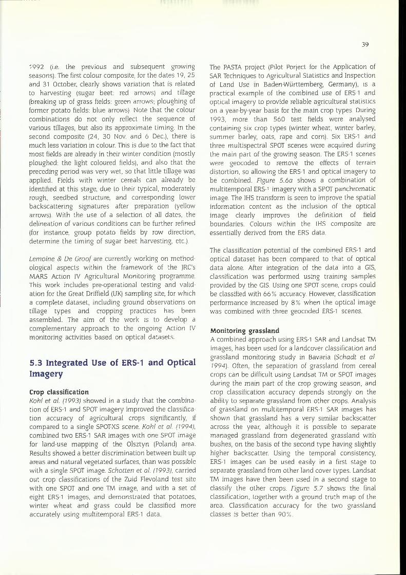
1992 (i.e. the previous and subsequent growingseasons). The first colour composite, for the dates 19, 25and 31 October, clearly shows variation that is relatedto harvesting (sugar beet: red arrows) and tillage(breaking up of grass fields: green arrows; ploughing offormer potato fields: blue arrows). Note that the colourcombinations do not only reflect the sequence ofvarious tillages, but also its approximate timing. In thesecond composite (24, 30 Nov. and 6 Dec.), there ismuch less variation in colour. This is due to the fact thatmost fields are already in their winter condition (mostlyploughed: the light coloured fields), and also that thepreceding period was very wet, so that little tillage wasapplied. Fields with winter cereals can already beidentified at this stage, due to their typical, moderatelyrough, seedbed structure, and corresponding lowerbackscattering signatures after preparation (yellowarrows). With the use of a selection of all dates, thedelineation of various conditions can be further refined(for instance, group potato fields by row direction,determine the timing of sugar beet harvesting, etc.).

Lemoine & De Graaf are currently working on method­ological aspects within the framework of the JRC'sMARS Action IV Agricultural Monitoring programme.This work includes pre-operational testing and valid­ation for the Great Driffield (UK)sampling site, for whicha complete dataset, including ground observations ontillage types and cropping practices has beenassembled. The aim of the work is to develop acomplementary approach to the ongoing Action IVmonitoring activities based on optical datasets.

5.3 Integrated Use of ERS-1 and OpticalImagery

Crop classificationKohl et al. (1993) showed in a study that the combina­tion of ERS-1and SPOTimagery improved the classifica­tion accuracy of agricultural crops significantly, ifcompared to a single SPOT-XSscene. Kohl et al. (1994),combined two ERS-1SARimages with one SPOTimagefor land-use mapping of the Olsztyn (Poland) area.Results showed a better discrimination between built-upareas and natural vegetated surfaces, than was possiblewith a single SPOTimage. Schotten et al. (1993), carriedout crop classifications of the Zuid Flevoland test sitewith one SPOT and one TM image, and with a set ofeight ERS-1 images, and demonstrated that potatoes,winter wheat and grass could be classified moreaccurately using multitemporal ERS-1data.

39

The PASTAproject (Pilot Porject for the Application ofSARTechniques to Agricultural Statistics and Inspectionof Land Use in Badenwurttemberg, Germany), is apractical example of the combined use of ERS-1 andoptical imagery to provide reliable agricultural statisticson a year-by-year basis for the main crop types. During1993, more than 560 test fields were analysedcontaining six crop types (winter wheat, winter barley,summer barley, oats, rape and corn). Six ERS-1 andthree multispectral SPOT scenes were acquired duringthe main part of the growing season. The ERS·1sceneswere geocoded to remove the effects of terraindistortion, so allowing the ERS-1and optical imagery tobe combined. Figure 5.6a shows a combination ofmultitemporal ERS-1imagery with a SPOTpanchromaticimage. The !HS transform is seen to improve the spatialinformation content as the inclusion of the opticalimage clearly improves the definition of fieldboundaries. Colours within the !HS composite areessentially derived from the ERS data.

The classification potential of the combined ERS-1andoptical dataset has been compared to that of opticaldata alone. After integration of the data into a GIS,classification was performed using training samplesprovided by the GIS.Using one SPOTscene, crops couldbe classified with 66 % accuracy. However, classificationperformance increased by 8% when the optical imagewas combined with three geocoded ERS-1 scenes.

Monitoring grasslandA combined approach using ERS-1SARand Landsat TMimages, has been used for a landcover classification andgrassland monitoring study in Bavaria (Schadt et al.1994). Often, the separation of grassland from cerealcrops can be difficult using Landsat TM or SPOTimagesduring the main part of the crop growing season, andcrop classification accuracy depends strongly on theability to separate grassland from other crops. Analysisof grassland on multitemporal ERS-1 SAR images hasshown that grassland has a very similar backscatteracross the year, although it is possible to separatemanaged grassland from degenerated grassland withbushes, on the basis of the second type having slightlyhigher backscatter. Using the temporal consistency,ERS-1 images can be used easily in a first stage toseparate grassland from other land cover types. LandsatTM images have then been used in a second stage toclassify the other crops. Figure 5.7 shows the finalclassification, together with a ground truth map of thearea. Classification accuracy for the two grasslandclasses is better than 90 % .

40

Figure 5.6a. ERS-1multitemporal colour composite, Baden-Wiirttemberg test site, Germany, 1993.Red: 20 May, green: 24 June,blue: 29 September. (Source: Hartl & Klaedtke 1994).

Figure 5.6b. /HS colour composite produced by combining ERS-1 imagery acquired on 20 May, 24 June and 29 July 1993with a panchromatic image acquired on 1 April 1993, Bodenwurttemberg test site. (Source: Hartl & Klaedtke 1994).

41

42

The Result of a Combined Laud use Classification of Multitemporal ERS-1 SLC Data of the Year 1992and a LANDSAT TM Image ofMay,28th 1992in Comparison to the Digital Ground Truth Map

Classification Result Digital Grotmd Truth Map

- forest- water- buildings I urbanareas- grassland

c:::::J grasslandwith bushesc:::::J oatsc:::::J wlnterwheat- summerbar1ey

-comc::J rapeseed- set- aside arablelandc:::=i gravelwork

- opensoil I peatworkc:::=i special landuse- not classified

Figure5.7. Theresult of a combined landuse classification using multitemporal ERS-1SLCimagery and a Landsat-TMimage 1992.The digital ground truth map is shown for comparison.

6. Tropical Crops

6.1 Rice

6.1.1 General

Socio-economic importance of riceRice is the prime source of daily food for those twothirds of the world's population living in Asia. Table 6.1shows the major rice producing countries, including ~selected European countries. For some countries rice a::export is an important source of income. Thailand, forexample, exports about one third of its annualproduction, which makes it the main supplier on theworld rice market. The production of rice contributes tosocial and political stability within the country.Consequently, decision makers have placed thecollection of information about the actual and predictedstate of rice crops on the top of their political agendas.

The most interesting parameters to know are riceacreage and potential yield. Currently, the collection ofthis information is mostly based on interviews of thefarmers or village level. The information gatheringprocess is cumbersome, and sometimes unreliableinformation is given to Government authorities by thelocal farmers. An objective method of data collection -such as based on the use of satellite imagery - istherefore of high interest for the national authoritiesdealing with agricultural economics and planning. Sincerice grows mostly in tropical countries, permanentcloud coverage during the growth period - whichnaturally coincides with the rainy season - is a majordrawback for the use of optical satellite imagery. As analternative, the use of radar remote sensing was

Table 6. 1 Rice production of the leading rice producing countries and selected European countries (numbers in1OOOsof metric tons; source: Electromap Inc., 1989·93)

43

120·dayVariety

,,,,,,',

Country Rice production Country Rice production Country Rice production(Top 12) IX 1000 t) (Top 12) (x 1000 t) (Europe) (x 1000 t)

1. China 187,450 7. Myanmar 13,201 Italy 1,2362. India 110,945 8. Japan 12,005 Spain 5823. Indonesia 44,321 9. Brazil 9,503 Portugal 1534. Bangladesh 28,575 10. Philippines 9,670 Greece 1275. Thailand 20,040 11. S·Korea 7,478 France 1096. Vietnam 19,428 12. USA 7.006 Hungary 38

,,

Olc"6Q)Q)(j)

Ol Days from Sowing to Harvestc-~coa.Cf)

ccof-'=

UiQ)>roI

120 days

c0

Q) ..:::;- cog Ec ~co 00... LL

Olciii:;:0u::

I I r

Reproductive RipeningVegetativePhase Phase Phase

55 days 35 days 30 days

Figure 6.1. Phenological stages of rice plant growth for atypical period of 120 days.

demonstrated to be an excellent means for repetitivecollection of information related to rice acreage and,even one step further, parameters related to rice yield(Aschbacher et al., 1995a).

44

Phenological stages of rice plant growthA typical rice growth cycle lasts between 120-180 daysfrom planting to harvest, depending on crop variety.There are three major plant growth phases: thevegetative, reproductive and ripening phase. After soilpreparation rice fields are flooded. The vegetative phasestarts either with direct sowing or transplanting ofnursery plants. During this phase young plants emergefrom the water surface.

During the reproductive phase, plants continue to growuntil they reach a maximum height of about one metre.During the ripening phase, the grains develop. Water isnormally drained out and the plants become drier andturn yellow. The reproductive and ripening phases areconstant for most varieties and last about 35 and 30days, respectively. The length of the vegetative phasediffers with variety. After harvest a bare soil conditionremains, sometimes with patches of standing water left.A typical phenological development of the rice plantduring its growth cycle is shown in Figure 6. 1.

There are glutinous and non-glutinous, photo sensitiveand non-photo sensitive, as well as resistant and lessresistant crop varieties. In recent years short-cycledvarieties are favoured, which allow an increased pro­duction through more frequent harvests. In intensiverice producing areas such as in Thailand the typicalgrowth cycle lasts 120 days. Crop yield depends on cropvariety and water availability. A typical crop yield for awell irrigated field is approx. 5 tons/ha. The availabilityof water during the early growth stage is crucial, whichhas led to the development of sophisticated irrigationnetworks in most of the intense rice growing areas(Aschbacher & Paudyal, 1993).

Radar remote sensing studies for rice crop mappingand monitoringFrom an agro-economic point of view there are twomain parameters of interest, namely (i)rice acreage, and(ii) rice yield. Rice production of a given area can beobtained as the product of acreage and yield (per unitarea). As will be shown later in this Chapter, it is easierto retrieve acreage from radar imagery than yield.

The investigations of ERS-1SARdata for rice monitoringinclude studies carried out in Thailand (Aschbacher &Paudyal, 1993; Paudyal, 1994), in Indonesia (Asch­bacher et al., 1995; Harms, 1993), in Spain (Kohl et al.,1993) and in Japan (Kurosu et al., 1993). Earlier studiescarried out before the launch of ERS-1are from Le Toan(1989) based on X-band scatterometer measurements,and Aschbacher & Lichtenegger (1990) based on SIR-Al.band data.

The Thailand and Indonesia studies are described indetail in this Chapter, while the studies carried out inSpain and Japan are also included for comparison withthose of the tropical countries.

Multitemporal radar backscattering signaturesWith reference to § 3.3, the radar backscatteringcoefficient a0 idB] of rice fields undergoes a verycharacteristic temporal signature during the growingseason. Compared to other agricultural crops, thetemporal signature of rice fields is probably the mostsignificant one showing the largest changes in radarbackscattering values during the growing period. This iscaused by the changing influence of macroscopic radarbackscattering interactions between standing water andplant canopy. A schematic temporal backscatteringprofile has previously been shown (§ 3.3.), and realvalues as observed with ERS-1SARdata are shown in§ 6.1.2 and 6.1.4, respectively.

6.1.2 Case studies in ThailandSome of the most detailed case studies on the use ofERS-1SARdata were carried out in Thailand (Paudyal,1994; Aschbacher et al., 1994, 1995a). Twomain studyareas were used, both of which are located east of thetown of Kanchanaburi, Thailand. Although both areasare only about 30 km apart the characteristics of therice fields are quite different. The northern area showsslightly undulating terrain, with small individual ricefields and a heterogeneous growing pattern betweenneighbouring fields, The southern study area is flat withlarge individual fields and a generally homogeneousgrowing pattern. In both areas a well developed irriga­tion network provides sufficient water for rice growth.The southern site is part of the EC-ASEANERS-1project,described in Aschbacher (1992).

For both studies, multitemporal ERS-1 SAR data wereavailable from nine acquisition dates, namely 22 Nov91, 7 Oct 92, 11Nov 92, 24 Feb 93, 7 May 93, 11 jun 93,20 Aug 93, 29 Oct 93 and 3 Dec 93. The 1991/92 datesare mostly used for the northern study area, while alldates are used for the southern study area.

Detailed ground measurements were carried out forboth study areas. During the rice growth period(June- December 1993), the ground measurementsdescribed in Table 6.2 were taken in parallel with ERS-1acquisitions. Ten different sample areas were selectedfor detailed investigations, each of them approximately1- 2 hectares in size.

45

Table6.2 Ground measurements taken in parallel with ERS-1SARdata acquisitions during June-December1993 atthe southern study area in Kanchanaburi, Thailand (Aschbacher et al, 1995).

Parameter Details

GPSand topographic mapLocation deg lat/long

Site photograph state & geometry of rice plants and surface

Method

square grid behind plant

General information Site acreage/planting method (seeding/transplantiflgl. variety name,date of planting, date of harvest, yield, irrigation (rainfed/irrigatedl

measurements and farmer in·terviews

Weather at acquisitiontime

wind (heavy/medium/light/no), plant orientation (vertical/bended-inwhich direction), rainfall (heavy/light/no), surface & plant condition

measured, visual inspection

state of plant growth soil preparation/vegetative stage/tillering/bo6ting/flowedng/panicle/ha.rves~ingstage

visual inspection

Plant parameters plant d@nsity,_plapt height, pli.lntrnoistu.recontent(weigrt beforeafter drying), no. of leaves, leaf width, leaf length, stalk diameter

rnTasurTct,avTrage .of1o sampleswithin 50 x 50 cm frame

Field information height of standing water, general state of surface, general state ofplants, .etc.

measurements, visual inspection

Estimate of rice acreageRice acreage can be retrieved from multitemporal radarimagery, making use of the characteristic backscatter­ing signature of rice fields. The temporal a0 !dBi profileof rice is unique, and thus quite easily distinguishablefrom that of other crops. The fact that rice fields areflooded during a certain period of time creates a clearsignature, namely that of a water surface during theearly growth period. Later, when plants are increasing inheight, backscatter increases to values which aretypically higher than those of other agricultural crops.The large dynamic range of a0 idBI between the early(flooded) and late (pre-harvest) growing period is animportant factor for rice mapping. It is, however, crucialto select optimum dates within this cycle. These areduring the early growing period when the surface isflooded, during the flowering phase and shortly beforeharvest. This corresponds to the minimum (approx.-16 dB), maximum (approx. - 8 dB) and (slightly de­creased) pre-harvest values of a0.

The growing cycle for the main rice harvest in the Kan­chanaburi study area lasts from August to December,and for a secondary harvest from April to July. A three­date multitemporal image combination is displayed inFigure 6.2, in which rice fields (in green/bluish colours)can easily be discriminated by visual interpretationfrom _other land-use categories. A digital classificationwas carried out based on four acquisition dates in orderto produce a 'rice map'. All images were co-registered

and Gamma MAP filtered (Nezry et al., 1995) before asimple clustering algorithm was applied.

The result is shown in Figure 6.3 for the three classes:'rice fields', 'non-rice fields', and 'water'. This clearlyindicates that the rice growing area is generally wellclassified. There is, however, some confusion with waterareas and the backslopes of mountains. Both effects canbe removed if GIS-type information is included in thefinal classification process (Aschbacher et al., 1995a).

Rice growth parametersThe ultimate goal in the use of radar imagery for ricestudies is to retrieve yield figures from satellite imagery.Currently, there are only two studies known which pointin this direction, one carried out in Japan (Kurosuet al.,1993) and one in Thailand (Aschbacher et al., 1995a).Both aim at yield-related parameters such as plantheight rather than yield itself. An example from the Thaistudies is shown in Figure 6.4, where measured plantheight is compared with radar backscattering values.Because the timing of rice planting is almost identicalfor different years, two more dates from previous yearshave been included, namely 22 Nov 91 and 7 Oct 92, inorder to complement some of the missing acquisitionsduring the 1993 growth cycle or the 'wind-disturbed'image of 20 Aug 93. As can be seen from Figure 6.4athere is a clear increase of radar backscattering valueswith increasing plant height. The mean ao values is-10.6 dB two months before harvest (with a spread

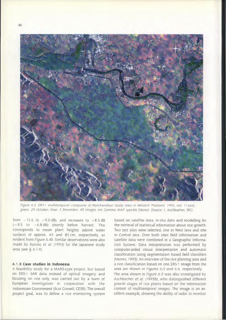
46

Figure 6.2. ERS·1 multitemporal composite of Kanchanaburi study area in Western Thailand, 1993; red: 11lune;green: 29 October; blue: 3 December. All images are Gamma MAP speckle filtered. (Source: 1.Aschbacher, IRC).

from -12.6 to -9.0dB), and increases to -8.5dB(- 9.5 to - 6.8 dB) shortly before harvest. Thiscorresponds to mean plant heights (above watersurface) of approx. 45 and 85 cm, respectively, asevident from Figure 6.4b. Similar observations were alsomade by Kurosu et al. (1993) for the Japanese studyarea (see§ 6.1.4).

6.1.3 Case studies in IndonesiaA feasibility study for a MARS-type project, but basedon ERS-1 SAR data instead of optical imagery andfocusing on rice only, was carried out by a team ofEuropean investigators in cooperation with theIndonesian Government (Scot Conseil, CESR).The overallproject goal, was to define a rice monitoring system

based on satellite data, in-situ data and modelling forthe retrieval of statistical information about rice growth.Two test sites were selected, one in West Java and onein Central Java. Over both sites field information andsatellite data were combined in a Geographic Informa­tion System. Data interpretation was performed bycomputer-aided visual interpretation and automaticclassification using segmentation based field classifiers(Harms, 1993). An overview of the rice planting area anda rice classification based on one ERS-1image from thearea are shown in Figures 6.5 and 6.6, respectively.The area shown in Figure 6.5 was also investigated byAschbacher et al. (1995b), who distinguished differentgrowth stages of rice plants based on the informationcontent of multitemporal images. The image is an ex­cellent example, showing the ability of radar to monitor

Figure 6.3. Classified 'rice map' based on four ERS-1acquisitions (6 fun., 20 Aug., 29 Oct. and 3 Dec. 1993).Rice is shown in mauve, non-rice areas in dark green and water in light blue. (Source:Aschbacher et al., 1995).

100 -Q.OI I I•~e ro ~.O

~ iii•.. 6) i::::i.cI --.!2'

GI.c 4) 'l>tc-a. 2)

,-14.0 -,

o•• I I , -16.016--Aug so-seo 14-Nov 29-Dec 16--Aug ~Sep 14-Nov 29-Dec

(a) (b)

Figure 6.4. Comparison of (a) changes in rice backscatter with time of rice fields in Kanchanaburi, Thailand (the ricegrowing period lasts from August to December); (b) rice plant height (above water) measured at the same sample fields.(Source:Aschbacher et al. 199Sa).

47

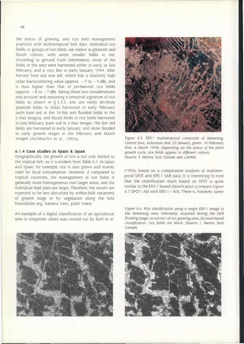
48

the status of growing, and rice field managementpractices with multitemporal SAR data. Individual ricefields, or groups of rice fields, are shown in greenish andbluish colours, with some smaller fields in red.According to ground truth information, most of thefields in the area were harvested either in early or lateFebruary, and a very few in early )anuary 1994. Afterharvest bare soil was left, which has a relatively highradar backscattering value (approx. - 7 to - 5 dB), andis thus higher than that of pre-harvest rice fields(approx. - 8 to - 7 dB). Taking these two considerationsinto account and assuming a temporal signature of ricefields as shown in § 3.3.3, one can easily attributegreenish fields to fields harvested in early February(with bare soil in the 16 Feb and flooded fields in the6 Mar images), and bluish fields to rice fields harvestedin late February (bare soil in 6 Mar image). The few redfields are harvested in early )anuary, and show floodedto early growth stages in the February and Marchimages (Aschbacher et al., 7995a).

6.1.4 Case studies in Spain & JapanGeographically, the growth of rice is not only limited tothe tropical belt, as it is evident from Table 6.1. In )apanand Spain, for example, rice is also grown and mainlyused for local consumption. However, if compared totropical countries, the management of rice fields isgenerally more homogeneous over larger areas, and theindividual field sizes are larger. Therefore, the results areexpected to be less disturbed by within-field variationsof growth stage or by vegetation along the fieldboundaries (e.g. banana trees, palm trees).

An example of a digital classification of an agriculturalarea in temperate zones was carried out by Kohl et al.

Figure 6.5. ERS-1 multitemporal composite of Semerang,Central Java, Indonesia (red: 23 January, green: 16 February,blue: 6 March 1994). Depending on the status of the plantgrowth cycle, rice fields appear in different colours.(Source: J. Harms, Scot Conseil and LAPAN).

(1993), based on a comparative analysis of multitern­poral SPOTand ERS-1SARdata. It is interesting to notethat the classification result based on SPOT is quitesimilar to the ERS-1based classification (compare Figure6.7 SPOT-AIS with ERS-1-AIS). There is, however, some

Figure 6.6. Rice classification using a single ER5·1 image ofthe Semerang area, Indonesia, acquired during the fieldflooding stage; (a) extract of rice growing area, (b)pixel-basedclassification, rice fields are black. (Source: J. Harms, ScotConseil).

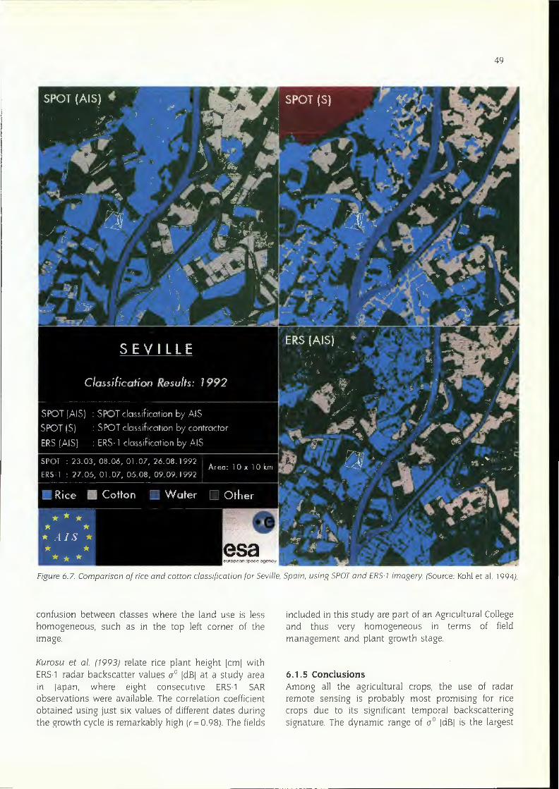
49

Figure 6.7. Comparison of rice and cotton classification for Seville, Spain, using SPOTand ERS·1 imagery (Source: Kohl et al. 1994).

confusion between classes where the land use is Jesshomogeneous, such as in the top left corner of theimage.

included in this study are part of an Agricultural Collegeand thus very homogeneous in terms of fieldmanagement and plant growth stage.

Kurosu et al. (1993) relate rice plant height [cm[ withERS-1 radar backscatter values a0 [dB[ at a study areain Japan, where eight consecutive ERS-1 SARobservations were available. The correlation coefficientobtained using just six values of different dates duringthe growth cycle is remarkably high (r= 0.98). The fields

6.1.5 ConclusionsAmong all the agricultural crops, the use of radarremote sensing is probably most promising for ricecrops due to its significant temporal backscatteringsignature. The dynamic range of a0 [dB[ is the largest

50

among all agricultural crops, ranging from approx.-16 dB during the flooded and early growing stage, toapprox. - 8 dB during the pre-harvest stage. The selec­tion of appropriate acquisition times is crucial formapping purposes. As regards yield estimates orparameters that lead to yield estimates, there is a clearcorrelation between radar backscattering signals andplant height. This allows the approximate age of riceplants to be determined, and thus a prediction of theapproximate harvesting time.

The results available from several case studies allow thefollowing conclusions to be drawn on the use of ERS-1SARdata for rice mapping and monitoring (Aschbacheret al., 1995a,b):1_ Multitemporal ERS-1 SAR data can be used in an

operational or quasi-operational mode for mappingof rice fields, both for irrigated and rain-fed fields.

2. Multitemporal ERS-1SARdata can be used in a pre­operational manner for the retrieval of yield-relatedparameters.

3. A priori knowledge about the rice crop calendar andgrowing practices as well as parallel in-situmeasurements largely facilitate the interpretation ofradar images. However, reliable results can beobtained without or with a very limited set of in-situmeasurements. This is of particular interest in viewof large-scale operational rice monitoring systems.

4. Formapping purposes, at least three dates should beavailable during the growing cycle. The optimumacquisition times are during the early flooded stage,the flowering stage and shortly before harvest. Anadditional post-harvest image is useful if the time ofrice harvest is different from that of other agriculturalcrops on the same scene.

5. For the retrieval of yield-related parameters the use of4 - 8 acquisitions during the growth cycle is recom­mended. The image dates should be equally spreadthroughout the growth period. An acquisition shortlybefore harvest is mandatory.

6. Multi-temporal ERS·1 SAR data can be used todetermine field management practices; such as thetiming of irrigation, time of harvest, method of watersupply (irrigated or rain-fed), and the length of thegrowth cycle. This information can be retrievedlargely without in-situ measurements.

7. As regards the optimum analysis technique appliedto radar imagery for rice mapping, it is recommend­ed to speckle filter the images and apply textureand/or segmentation based algorithms, beforeclassifying the images. Depending on the scenecharacteristics, special measures may have to beapplied if field management differs within one scene.

8. If an operational rice monitoring system isdeveloped, it is strongly recommended to includemultitemporal radar imagery as a prime data source.

Figure 6.8. ERS-1 image of part of Johar state, Malaysia, 24August 1993, coverage 100x100 km. (Source: M. Wooding,RSAC).

Figure 6. 9. ERS-1 PR! extract of Costa Rican coast, 18 May1992; banana plantations show the brightest returns,Gamma MAP filtered. (Source: M. Wooding, RSAC).

6.2 PlantationsERS-1images are potentially valuable for mapping sometypes of plantation crops, which form an important partof the economy of many tropical countries. Oil palmand bananas, in particular, tend to have very brightimage tones in comparison with other types of tropicalvegetation because of the large leaf sizes and the overallstructure of the vegetation.

Figure 6.8 is an ERS-1image covering parts of southernMalaysia and Singapore Island. Large oil palmplantations are seen as the lighter toned patches in thezone between the coastal plain and the mountains tothe north-east. The coastal plain itself is an area ofmixed smallholder agriculture without clear fieldpatterns, which has darker image tones. Besides thepotential for mapping new areas of oil palm, there isalso some interest for monitoring the replanting of oilpalm, which happens approximately every 30 years.Replanted oil palm appears dark on ERS-1 imagesbecause the signal is dominated by the low herbaceousground cover between young trees.

Banana plantations are readily seen on ERS-1 images,Beaulieu et al. (1994). Figure 6.9 shows large planta­tions in Costa Rica located on flat land near the coastand on large alluvial fans within the mountains. Bananaplantations are identified both by their brightness andgeometric shape. Although the extent of areascultivated with banana are relatively well known inCosta Rica, there is potential for monitoring changes inthe extent of plantations, which can be quite rapid insome areas.

51

6.3 Other CropsThere is a great variety of tropical agricultural crops,examples of which are rice, sugarcane, maize, tapioca,coffee, tea, rubber and fruit tree plantations. Rice andtree plantations have been discussed in § 6.1 and 6.2,respectively. Paudyal (1994) has investigated also otherland cover categories at the Thailand study area(described in § 6.1), where, apart from rice fields, largeplots of sugarcane are present, intermixed with bushes,shrubs, water and urban areas.

Various classification methods were compared such asmaximum likelihood with knowledge-based classifica­tion methods, or unfiltered versus speckle filteredand/or texture analysed images. The latter method wasdeveloped making use of pre-assumptions about therice growth cycle based on temporal profiles of o? !dBi.These results were compared with a Landsat TM imageand ground measurements for accuracy assessment.An overview of the classification results is given in Table6.3.

The results of the supervised classification based on fivedates (MAP-filtered)has given an overall classificationaccuracy of 70 % , while the knowledge-based methodgave 80 % , which is a clear improvement. The sameaccuracy was obtained when combining speckle andtexture analysed images as input for a maximumlikelihood classification. As an example, the classifica­tion accuracy matrix was extracted for the agriculturalcrops, rice and sugarcane only, and compared with theoverall accuracy including all six land cover categories.It is worth noting that the accuracy of rice alone hasincreased from 72 % for the MAP-filteredclassification to92 % for the knowledge-based segmentation method.

unfilteredMAP-speckle. filtered

(2 iterat.)4

segmentation

age dates. Theobservedne, bush, shruhs, water

70 7278 88

71

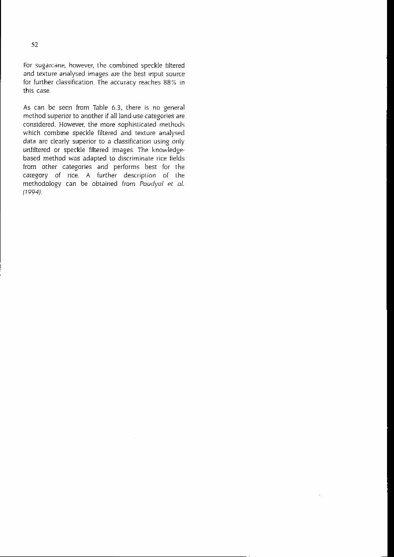
52

For sugarcane, however, the combined speckle filteredand texture analysed images are the best input sourcefor further classification. The accuracy reaches 88 % inthis case.

As can be seen from Table 6.3, there is no generalmethod superior to another if all land-use categories areconsidered. However, the more sophisticated methodswhich combine speckle filtered and texture analyseddata are clearly superior to a classification using onlyunfiltered or speckle filtered images. The knowledge­based method was adapted to discriminate rice fieldsfrom other categories and performs best for thecategory of rice. A further description of themethodology can be obtained from Paudyal et al.(1994).

53

7. Future Developments

7. 1 Data Continuity

Since its launch in 1991, ERS-1is the first radar satelliteto have provided a long period of continuous dataacquisition. ERS-1data have been used by the interna­tional science community since then to extractenvironmentally important parameters. Despite therestriction to a single frequency and polarization, theguaranteed high-repetition frequency and the sensor'squality and stability make it a very importantmonitoring tool. ERS-1 has acquired more than half amillion images, which will be exploited for years tocome. With the launch of ERS-2 in 1995 and Envisat in1998, there is the prospect of data continuity well intothe next century using ESA satellites. Other radarsatellites including JERS-1 and Radarsat will furtherextend the amount of data. Brief technical specificationsfor these satellite radar systems are given in Table 7.1.

Built like ERS-1, ERS-2 carries the same active radarinstruments to continue the data flow started in 1991.For a period of time, it is planned to operate bothspacecraft 'in tandem' to collect interferometric datapairs (see § 4.5 and 7.3). One of the main applicationsof interferometry is to develop three-dimensional digitalmaps of the Earth's surface. The C-band data continuitywill be guaranteed with the ASAR (advanced SAR)system on-board the Envisat platform. The Envisatmission will be ESA'sthird major remote sensing effort.As ERS-1/2, it will use a polar orbit at 800 km altitudeand 98.5° inclination. Based on the Polar Platformconcept, Envisat carries ten active instruments to covera wide range· of remote sensing tasks from Earth'ssurface monitoring to atmospheric research.

Table 7. 1 Continuously operating and planned spaceborne SAR systems

Sensor ERS-1 ERS-2 Envisat JERS-1 Radarsat

Agency ESA ESA ESA NASOA CSALaunch 1991 1995 1999 1992 1995Expected lifetime 3 years 3 years 5 years 2 years 5 yearsFrequency (GHz) 5.3 5.3 5.3 1.3 5.3Polarisation vv vv VV, HH, VH HH HHIncidence angle 23 23 15 to 55 38 1O to 60Range resolution 26 26 30 18 9 to 1ooAzimuth resolution 28 28 30 18 9 to 100

The Japanese spaceborne SARprogramme started witha SAR on JERS-1 (Japanese Earth Resources Satellite).Application objectives focused on Earth resources andenvironmental protection, disaster prevention andcoastal monitoring. In contrast to the other systems,JERS-1allows observation at L-band (23 cm wavelength),supplying additional information about the Earth'ssurface. Figure 7.1 illustrates a comparison of ERS-1and)ERS-1SARimages over the Dutch Flevoland agriculturalsite (Borgeaud et al., 1994).

The Canadian Radarsat adds, by using HH-polarization,an additional feature to the available radar parameters.It is also capable of beam steering, allowing varyingincidence angles and geometric resolutions (fineresolution vs. wide swath). The SAR data will bedistributed to commercial, government and scientificorganizations for applications in resource management,ice mapping and reconnaissance and environmentalmonitoring.

7 .2 Multi-parameter Radar

The useful information which a satellite radar canprovide on an agricultural field depends on the kinds ofstructures within the crop canopy or the soil with whichit interacts. The natures of those structures and thestrengths of interaction are influenced by theparameters of the radar, including its frequency andpolarisation (Schmullius & Nithack, 1992). A multi­channel radar exploits these differing responses toprovide a more complete instantaneous picture of thestructure or density of a crop.

Figure 7. 1 Comparison of (a) ERS-1 and (b) /ERS-1!SAR images over the Dutch test site, Flevoland (Source: M. Borgeaud,ESA/ESTEC)

54

(a)

Radar frequency is a tool for varying the penetration ofmicrowaves into the canopy of a crop. While, in somecircumstances, the C-band radiation of ERS-1 canpenetrate completely through a canopy, it is notgenerally as penetrative as longer wavelengths such asL- band. Longer wavelengths react with structuresthrough a greater volume of a canopy, and moreregularly interact with the soil below. Higherfrequencies, such as X-band radars, are more sensitiveto the small-scale properties of the upper layers ofvegetation or the canopy boundary layer.

The selection of horizontal and vertical polarisationvaries the response of a radar to different shapes orscattering elements within a canopy. Selecting crossedpolarisations between the radar transmitter andreceiver, tends to detect backscatter from within thevolume of a crop canopy rather than from the soil, andas such may be an indication of the amount of biomass.We might conceivably select different single radarchannels or particular frequency and polarisationcombination to optimise the discrimination of certaincrops at some point in the growing season. Of fargreater potential, however, is the use of multiplefrequencies and/or polarisations simultaneously toprovide a multi-dimensional set of measurements, akinto moving from monochrome optical imagery to colour.

Airborne radar experiments over the last two decadeshave supplied the remote sensing user community with

(b)

high-quality multi-frequency and/or multi-polarizationdata (e.g. AGRISTARS,ROVE, AGRISCATT,AGRISAR,MAESTRO1, Mac Europe 91, EMAC-1994).The recentSIR-C/X-SAR1 and 2 experiments during April andOctober 1994 offered, for the first time, an opportunityto acquire multi-parameter SARdata from space withinthe 10-day mission time frame.

The application of multi-frequency SAR data for cropidentification is demonstrated in Figure 7.2, which is acolour composite of x-band, C-band and L-band imagescovering the same 2.5 x 6 km area as the multitemporalERS·1 composite shown in Figure 5.2. On the imagingdate in )uly, all crops are fully developed and causecharacteristic backscatter intensities, which simplifiesthe digital landuse classification. The brightest fieldsbelong to oilseed rape (yellow-white) and sugar beet(light orange), since they have the highest backscatterin all three wavelengths. Dark blue fields are winterwheat (higher L-band returns), green fields are summerbarley (higher C-band returns), making discriminationbetween cereals possible (compare the C-VV temporalsignatures in Figure 3.10).

Figure 7.3 shows a multi-frequency composite acquiredfrom the space borne SIR-C/X-SAR.The image wasacquired at 04:00 GMTat night, as a thick cloud layercovered Germany, and shortly after a heavy stormcovered the area with 20 cm of snow. The quality of theimage demonstrates the capabilities of radar remote

Figure 7.2. DLR ESAR multifrequency colour composite,CLEOPATRAtest site Lechfe/d, Germany, 14 fuly 1992; red: X­vv, green: C-VV,blue: L-HH. (Source: C. Schmullius, DLR).

sensing for environmental monitoring independent ofweather conditions. Forested areas appear in red,because the long I-band wavelengths penetrate thevegetation canopy and are scattered by tree trunks andbranches. Agricultural fields (mostly bare soil) appearblue in this April image, since the longer wavelengthsare forward scattered, i.e. away from the sensor, but the

55

X-band signals undergo diffuse scattering. Where thevegetation is taller, e.g. in the marshy areas at thenorthern tip of the large lake (Ammersee), L-and C-bandreturns add to the yellow colour.

Figure 7.4 provides an example of a C-band multi­polarisation composite. The airborne imagery wasacquired by the EMISAR system developed by theTechnical University of Denmark. It shows anagricultural area near Uppsala, Sweden, and is acomposite of HH, VVand HVpolarisation channels. Thelarge range of colour associated with the agriculturalfields provide a simple illustration of the extrainformation content of multi-polarisation radar, and isindicative of the future potential of Envisat with its dual­polarisation capability.

7 .3 Analysis Techniques

Neural networksDavison (1994) has investigated the potential of neuralcomputing techniques, which are being increasinglyapplied to a wide variety of classification applications,and are recognised to cope particularly well with 'noisy'data. Pixel-based neural network classification of multi­temporal ERS-1 data of the Great Driffield site, UK,produced an accurate classification result for a smallnumber of fields.

The work of Melis & Lazzari (1994) provides a furtherexample of the use of neural network classificationtechnique. Figure 7.5a is a multitemporal ERS-1/SARimage (April, May and July 1992) for a test site in theTiber Valley, Rome. Figure 7.5b is an unsupervisedclassification obtained by a neural network (3-dimen­sional Kohonen's Map).

SAR interferometrySAR interferometric data processing combines twocomplex valued images acquired with slightly differentsensor positions. For ERS-1imagery, random dislocationof the individual scatters between the two acquisitionsreduces the interferometric correlation. As a conse­quence, this correlation contains thematic informationwhich can be used to support land-use classificationand change detection (Wegmiiller et al., 1995).

A series of ERS-1/SAR SLCimages of an area near Bonn,Germany, have been analysed using interferometricmethods. The images were acquired in 3-day intervalsgiving good phase coherence between image pairs.Images acquired between 1 and 28 March were con­sidered, and a total of nine coherence images from thedifferent image pairs were generated.

56

Figure 7.3. SIR·CIXmultifrequency colour composite, Germany, 13April 1994; red: L·total power; green: C-total power;blue: X-VV.(Source: C. Schmullius, DLR).

Figure 7.6 shows the results of combining three of thecoherence images. Forest areas and highways have lowcoherence so they show up as dark areas. For forests,this can be explained by the well-known de-correlationdue to multiple scattering. For the 'smoother' highways,the amplitude of the reflected signal is too low forcoherence detection.

All fields with no change in coherence over the period7 -16 March 1994 appear black and white. Groundobservations at the time of image acquisition help toexplain the apparent changes in coherence betweenfields. The coloured fields result from different greyvalues in at least one of the image planes. The red fields

have low coherence in the green and blue image planesand, therefore, do not contribute to the perceived colour.This can be explained by cultivation activities. Red fieldswere ploughed in the period 13-19 March 1994 andtherefore had low coherence compared to the start ofcultivation. Yellowfields have no coherence in the blueimage plane as farming activities occurred after 13March. In the same manner, all other colours can beexplained.

It should be noted that not only farmer activities causede-correlation. Other factors such as rain, wind blowand irrigation can be involved. However, in the Germanstudy, growth-related loss of coherence can be ruled out

Figure 7.4. EM/SAR Cband multi-potarimetriccolour composite, Uppsala, Sweden, 23 June 1994; red: HV; green: HH; blue: VV.(Source: E. Attema, ESTEC).

as the crops were not experiencing rapid changes inproductivity.

In a similar study of BadenWilrttemberg, coherenceimages were generated from image pairs acquired

57

58

Figure 7.5a.Multitemporal ERS-1FDCcomposite, Tiber Valley,Rome in 1992; red: April; green: May; blue: July(Source: ). Lichtenegger, ESAIESRIN).

Figure 7.6. ERS-1multitemporal colour composite showingrepeat-pass interferometric correlation, near Bonn, Germany,1994; red: 7-10; green: 10-13; blue: 13-16March. Colouredfields indicate farming activities in the observed periodsmostly attributed to the effects of ploughing.

during the period March to September. In all cases, nofringe images or coherence images could be generated

Figure 7.Sb.Unsupervised classification obtained by a neuralnetwork (3-0 Kohonen'sMap) approach after feature extrac­tion and statistics computation.

due to the time interval of 35 days between consecutivepasses. This period was too large and de-correlationoccurred due to abundant changes in vegetation cover.

The potential of repeat-pass SARinterferometry for cropmonitoring has been investigated using ERS-1 imageryacquired over Flevoland The Netherlands, in 1991.Figure 7.7 shows a multitemporal composite of theinterferometric correlation which occurred betweenthree different time periods. The colours indicatedifferences in crop development and cultivationpractice. Most potato fields appear blue due to the highcorrelation only between 19 October and 9 November.Prior to this period, interferometric correlation was lowdue to harvesting and spraying. However, for somepotato fields, changes had already occurred between 19September and 4 October as indicated by the turquoisecolour (high green and high blue). The yellow fields (highred, high green) indicate that fields were mechanicallycultivated between 19 October and 9 November for theestablishment of winter crops. Corresponding explana­tions are valid for the other crops.

Figure 7.8 shows a multitemporal backscatter compo­site for the same site. It is much harder to interpret thecolour changes. Only minimal differences are observeddespite the fact that fields are undergoing cultivationand harvesting. For a more detailed appraisal of thiswork, see Wegmiiller & Werner (1995).

Figure 7.7. ERS-1multitemporal colour composite showingrepeat-pass interferometric correlation, Flevoland, 1991; red:19Sept.-4Oct. pair, green: 4-19Oct. pair, blue: 19Oct.-4Nov.pair.

Cropgrowth modelsAgricultural crop growth can be monitored by usingcrop growth models. However,often estimates of cropgrowth are inaccurate for non-optimal growingconditions. Remote sensing can provide information onthe actual status of agricultural crops, thus calibratingthe growth model for actual growing conditions.Encouraging results have already been obtained usingoptical remote sensing data in estimating the leaf areaindex (LAI) regularly during the growing season andsubsequently calibrating the growth model on time­series of estimated LA!s.

59

Figure 7.8. ERS-1multitemporal backscatter colour compo­site, Flevoland 1991; red: 19Sept.; green: 4 Oct.; blue: 9Nov.(Courtesy of U. wegmuller, RSL).

By combining the SUCROScrop growth model for sugarbeet (Bouman, 1992), with microwave and opticalremote sensing data, it was possible to improve thepredicted yield. As shown in Table 7.2, the average erroron the crop yield is smallest when L-band SAR datatogether with an optical model are used to calibrate theSUCROScrop growth model.

Table 7.2 Average errors in yield estimation for sugar beet using a vegetation growth model calibrated either bymicrowave and/or optical data.

Techniques Error (tons/ha) Error(%)

SUCROS(vegetation growth model) 13.4 19.1SUCROSwith radar data (L-HH) 10.8 15.4SUCROSwith radar data (C-VV) 6.5 9.2SUCROSwith optical remote sensing data (3 dates) 4.0 5.7SUCROSwith radar data (C-VV) and optical model 3.7 5.3SUCROSwith radar data (L-HH)and optical model 3.3 4.7

61

8. Conclusions and Recommendations

8. 1 ERS-1 Backscatter of AgriculturalCrops

There have been significant developments in ourunderstanding of the radar backscatter of agriculturalcrops over the lifetime of ERS-1.Prior to the launch ofERS-1 in July 1991, research experience had concen­trated on experimental programmes using airborneradar systems, and involvement in space had beenlimited to brief duration Seasat and Shuttle ImagingRadar (SIR-Aand SIR-B)missions. The availability offrequent and reliably timed satellite radar data fromERS-1 has provided new insights into the potential ofmultitemporal radar imaging for monitoring agriculturalcrops. The excellent stability of the ERS-1/SARcalibration has been another important factor, facilitat­ing comparisons of crop backscatter measurementsacross different test sites and over different years.

Research work carried out within the ESAAnnounce­ment of Opportunity Programme has included studiesin successive years at test sites in The Netherlands, UKand Germany. In general there is very good correspon­dence in the backscatter of crops across the differenttest sites. It has been found that cereal crops (wheat andbarley) consistently show trends in backscatter as afunction of time. The main features are:

(i) a decline in backscatter during the tillering to theflag leaf stage

(ii) a period in which backscatter is at a minimum atthe time of heading and ear development

(iii) an increase in backscatter during grain fill untilharvest.

The backscatter minima which occurs at the headingstage is a characteristic which shows up consistently. Asbarley matures before wheat, the backscatter profilesfor barley appear to turn earlier and this provides abasis for separating these different cereal crops.

Rice also has been shown to have a characteristic tem­poral behaviour. In this case there is low backscatter atthe early stage of development associated with thepresence of standing water, backscatter increases toreach a maximum at the heading stage, and thendeclines slightly during senescence and harvest.

Environmental and meteorological effects have beenfound to have some influence on the crop backscatter.Wet crop conditions following rainfall seem to be themain factor, and this can result in an increase inbackscatter by several dB's. This suggests the need forancillary information on the timing of rainfall events.

RecommendationThe establishment of crop backscatter databases whichinclude both field averaged backscatter measurementsand details of crop growing conditions at the time ofERS-1 acquisitions. This is vital for improving ourgeneral understanding of causative relationships, andalso the effects of specific environmental/meteorolo­gical factors (e.g. rainfall, disease, drought, wind blow).A better understanding of the interaction of electro­magnetic waves with different crops is important forimproving current backscatter models.

8.2 Crop Classification

The fact that particular crops have distinctive temporalbackscatter profiles can be exploited for crop classifica­tion purposes. Rice, wheat, barley, oilseed rape andgrass have been shown to have particularly distinctivebehaviour. Time windows exist in which these crops areseparable on the basis of their backscatter anddifference in backscatter between dates, and this allowsthese crops to be classified with high orders of accuracy.Best results have been achieved using a field-basedapproach to classification. However, good results arealso possible using a pixel-based approach, where thisinvolves the use of special filtering or segmentationtechniques.

Often there is an important requirement to distinguishcrops at the earliest possible stage in the growingseason so that field checks can be performed wellbefore harvest. Results from Holland and the UKindicate that winter wheat can be accurately classifiedin early May and June (classification accuracies of> 80 % ). Oilseed rape can be mapped to accuraciesapproaching 100% using images from within the sametime frame. However, more difficulties have beenexperienced with the separation of sugar beet andpotato crops. Barley crops can be distinguished at the

62

end of June and early July. At this time barley ripensrelative to wheat and this is reflected in the temporalprofiles. Grass can only be distinguished usingadditional images acquired after the more seasonalcrops are harvested.

Results from Holland indicate that surface roughness inautumn is an indicator of site specific tillage andcropping practices in the following growing season.Although crop development is insignificant in Autumn,experimental results have shown that information couldbe obtained which was relevant to crop type discrimina­tion much later in the growing season. There seems tobe potential to use a combination of autumn and springimages to map crops earlier than would be possibleusing optical imagery.

Mapping of rice fields is also possible at a very earlystage when fields are flooded, which coincides withsowing or transplanting.

The potential for crop classification may be limited inareas where field sizes are very small. The accuracy ofaveraged field backscatter measurements is reduced forfield sizes less than 1 ha, and it becomes difficult toresolve individual fields of this size. However, this hasnot been a significant problem for rice mapping becauseof the common management of groups of fields relatedto water availability. Another important consideration isthe effect of geometric distortion in hilly areas. Much ofthe preliminary work has been carried out in areaswhere terrain distortion is not a problem (ie.East Angliain the UK,Lechfeld in Germany, the Dutch Polders andKanchanaburi in Thailand).

RecommendationFurther research studies are required to investigate cropclassification accuracies for a wide range of crops indifferent environmental situations. New work is requiredto assess the effect of local incidence angle correctionon crop classification performance in hilly terrain. Thereshould be an emphasis on the potential for early cropforecasts.

8.3 Strategies for Operational Use ofSatellite Radar Data

The main weakness of current crop monitoring systemsbased on the use of optical satellite data is the un­reliability of image acquisitions in parts of the worldwith frequent cloud cover. However, even when opti­mally timed images are available, there still appears to

be problems with the identification of some crops. TheSPOTsatellite for instance still lacks a spectral channelin the middle infrared which provides much approvedcrop discrimination (a situation that will change withthe launch of SPOT-4).

Although it is attractive to contemplate the use ofsatellite radar data for operational crop monitoringsimply on the basis of reliable cloud-free data acquisi­tion, the major issue is the value of the data for cropclassification in comparison, or used in conjunctionwith optical data. The research results on ERS-1 cropclassification presented in this document are viewed asbeing highly encouraging in this respect, and two alter­native approaches are suggested depending on thedifficulties encountered in obtaining optical satelliteimages.

Firstly, in cloudy parts of the world, such as the humidtropics and northern Europe, multitemporal satelliteradar data should increasingly fulfil a primary role,supplemented by occasional optical images. In thiscase, optical images would be used for field areameasurement and to aid in the classification of cropswhich are poorly discriminated on radar images.

Secondly, in parts of the world with generally clearweather conditions, optical satellite images shouldcontinue to be the main data source, althoughsupplemented by satellite radar images if these can beshown to be useful for early crop identification, or fordealing with particular crops which are difficult toclassify using optical images. Examples have beenpresented which show that classification performancecan be improved by the combined use of optical andERS-1 imagery.

Experience with ERS-1has established the potential ofsatellite radar for agricultural applications. With ERS-2,JERS-1,Radarsat (launch in 1995), and ASAR(launch in1998) providing continuity of data into the next century,there are excellent opportunities for exploiting thepotential of satellite radar for operational cropmonitoring in Europe and the rest of the world.Operational multi-frequency, multi-polarisation radarsnow being planned for early next century will extendthe capabilities even further. The potential for cropgrowth monitoring is likely to be improved both by theavailability of multi-frequency and multi-polarisationdata, and by the further development of interferometrytechniques. For rice there are already very positive yieldprediction results.

63

RecommendationsA programme of pilot projects should be initiated todevelop methodologies and to evaluate crop classifica­tion accuracies using ERS-1/2 data in different agricul­tural situations. There is also a need for more detailedanalyses of radar backscatter time series linked to cropgrowth models. These should be carried out within theframework of present remote sensing control andstatistics projects within Europe and elsewhere.

Finally, after four years of research and encouragingresults, operational users should be encouraged tointegrate ERS-1 imagery into their programmes.

Furthermore, the complementarity of optical and radardata should be studied in more detail as well as thepossibility of combining ERS and JERSdata.

65

9. References

Aschbacher J, 1992. Can satellites help in the management oftropical ecosystems? Proc. Intl. Space Year, Regional Seminaron Remote Sensing Applications to Tropical Eco-SystemManagement, Khao Yai, Thailand, 14-20 June 1992, ESCAP/UNDP,pp. 90-92.

Aschbacher J & Lichtenegger J, 1990. Complementary natureof SARand optical data: a case study in the Tropics,ESAEarthObs. Quart., Sept. 1990, No. 31, pp. 4·8.

Aschbacher J & Paudyal D R, 1993. Studies of rice fields inThailand using ERS-1 SAR data, Proc. National Conf ERS-1ILandsat/SPOT Applications: A Complementary Approach,Jakarta, Indonesia, 23-25 November 1993, p. 9.3. 1-9.3.9.

Aschbacher J, Dipak R P, Pongsrihadulchai A, Karnchanasu­tham S & Rodprom C, 1994. Radar backscattering studies ofrice fields using ERS-1SARdata, Proc. IGARSS 94, Pasadena,California, 10-12 August 1994.

Aschbacher J, Pongsrihadulchai A, Karnchanasutham S,Rodprom C, Paudyal D R & Le Toan T, 199Sa. Assessment ofERS-1SARdata for rice crop mapping and monitoring, Proc.IGARSS 95, Florence, Italy, 10-14 August (Abstract submitted).

Aschbacher J, Poniman A. & Wismann V, 1995b. Assessmentof ERS-1/SAR for tropical land-use mapping along coastalzones in Indonesia, Proc. IGARSS 95, Firenze, Italy, 10-14 Aug.(Abstract submitted).

Askne J& Hagberg J, 1993. Potential of interferometric SARforclassification of land surfaces, Proc. IGARSS 93, Tokyo, Japan,pp. 985-987.

Beaulieu N, Leclerc G, Velasquez S, Pigeonnat S, Gribius N,Escalant J-V& Bonn F, 1994. Investigations at CATIEon thepotential of high-resolution radar images for monitoring ofagriculture in Central America, SAREX-92 Workshop Proc.,Paris, 6-8 December 1993, ESAWPP-76, pp. 139-153.

Borgeaud M, Noll J & Bellini A, 1994. Multitemporal com­parisons of ERS-1and JERS-1/SAR data for land applications,Proc. IGARSS 94, Pasadena, CA, 10-12 Aug. 1994.

Bouman BAM, 1992. Linking physical remote sensingmodels with crop growth simulation models applied for sugarbeets, Intl. fl. of Remote Sensing, Vol.13, No. 14, pp.2565-2781.

Davison M, 1994. Development of neural network techniquesfor the classification of multitemporal ERS-1/SAR imagerywith respect to agricultural applications. Proc. 1st Workshopon ERS-1Pilot Projects, Toledo, Spain, June 1994, ESASP-365,pp 469-473.

Frost VS, Stiles JA, Shanmugan KS & Holztman JC, 1982. Amodel for radar images and its application to adaptive digitalfiltering of multiplicative noise, IEEE Trans. on PatternAnalysis and Machine Intelligence, Vol.PAMI-4, No. 2,pp. 157-165.

Geudtner D, 1995. Die interferometrische Verarbeitung vanSAR Oaten des ERS-1,DLR Forschungsbericht (in press).

Groot J,Van der Broek B,Nieuwenhuis G,Schotten C,Van RooijW & Jansen L, 1994. Crop classification using ERS-1/SAR data,Experts Meeting, JRC-IRSAAgricultural Project, 7-8 Feb. 1994.

Harms J, 1993. Integration of ERS-1 data into the Europeanproject of agriculture statistics, Proc. 1st ERS-1Symp., Cannes,France, 4-6 Nov. 1992, ESASP-359, Vol.2, pp. 629-630.

Harms J, Galaupe M, Rabaute T, Cailton JM, Roques j M &Demailly C, 1994. Integration of ERS-1data into the Europeanproject of agricultural statistics, Proc. 2nd ERS-1 Symp.,Hamburg, 11-14 Oct. 1993, ESA SP-361, Vol.1, pp. 85-86.

Hartl P & Klaedtke H G, 1994. Some results of the PASTAproject concerning agricultural classification, Proc. 1st Work­shop on ERS-1 Pilot Projects, Toledo, June 1994, ESASP-365,pp. 481-491.

Hartl P, Klaedtke H-G, Reich M & Xia Y, 1994. Agriculturalimplications of ERS-1 data: Preliminary results of the PASTAproject, Proc. 2nd ERS-1 Symp., Hamburg, 11-14 Oct. 1993,ESASP-361, Vol.1, pp. 63-68.

Iutten C, Blayo F, Cabestany J, Cheneval Y, Cowman P &Verleysen M, 1995. Eds. 'ELENA- Enhanced Learning forEvolution Neural Architects', ESPRITIII Basic Research Action(No.6891 ), Project Results and Industrial Openings, Brussels.

KohlH-G,1994. An evaluation of ERS-1PR!data in the contextof the rapid estimation of crop acreages in Europe, Proc.IGARSS 94, Pasadena, CA, 10-12 Aug. 1994.

Kohl H-G,King C & De Graaf H, 1994a. Agricultural statistics:Comparison of ERS-1 and SPOT for the crop acreageestimation of the MARS project, Proc. 2nd ERS-1 Symp.,Hamburg, Oct. 1993, ESASP-361 (Jan. 94), Vol.1, pp. 87-92.

Kohl H-G, Nezry E, De Graaf H & Kattenborn G, 1994b.Monitoring agricultural surfaces using ERS-1 multitemporalSAR data, Proc. IGARSS 94, Pasadena, CA, 10-12 Aug. 1994.

Kohl H-G,Nezry E, Mroz M & De Graaf H, 1994c. Towards theintegration of ERS/SARdata in an operational system for therapid estimate of crop acreage at the level of the EuropeanUnion, Proc. 1st ERS-1Pilot Projects Workshop, Toledo, Spain,ESASP-365, pp. 433-441.

66

KurosoT,Suitz T,Fujita M, ChibaK& Mariya T,1994.Ricecropmonitoring with ERS-1/SAR: a first year result, Proc. 2ndERS-1 Symp., Hamburg, ESASP-361,Vol. 1, pp. 97-102.

Laur H, Sanchez I. Dwyer E & Meadows P, 1993. ERS-1/SARradiometric calibration, Proc. SAR Calibration Workshop, ESAWPP-48,pp. 257-281.

LeeJS, 1986. Speckle suppression and analysis for syntheticaperture radar images,Optical Engineering, Vol.25, No.5, pp636-643.

Lemoine GG & De Groot H, 1994. Personal communication.

LeToanT,Laur H & Mougin E, 1989. Multitemporal and dual­polarisation observations of agricultural vegetation coversbyXband SAR images, IEEE Trans. on Geoscience & RemoteSensing, Vol.27, No.6, pp. 709-718.

Li Chang, 1988. Two adaptive filters for speckle reduction inSARimages using variance ratio, Intl. fl. of Remote Sensing,Vol.9, No.4, pp. 641-653.

LopezA, Nezry E,Touzi R& Laur H, 1993. Structure detectionand statistical adaptive speckle filtering in SARimages, Intl.fl. of Remote Sensing, Vol. 14, No.9, pp. 1735-1758.

Massonnet D,RossiM, Carmona C,Adragna F, PeltzerG,Feig!K & Rabaute T, 1993. The displacement field of the Landersearthquake mapped by SARinterferometry, Nature, No.364Vol.6433, 8 July 1993, pp. 138-142.

Meadows PJ & Wright PA, 1994. ERS-1SAR analogue todigital convertor saturation, Proc. SAR Calibration Workshop,CEOSCalibration/Validation Working Group, Ann Arbor, Ml,Sept.1994.

Melis M & Lazzari A, 1994. Multitemporal and single-imagefeatures extraction from ERS-1 image data with wavelettransforms and unsupervised neural networks, Proc. 1st ERS-1Pilot Projects Workshop, Toledo,June 1994, ESASP-365.

Nezry E, LopesA & TouziR, 1991.Detection of structural andtextural features for SARimage filtering. Proc. IGARSS 91, pp.2169-2172.

Nezry E, LeysenM & De Grandi G, 1995. Speckle and scenespatial estimators for SARimage filtering application to ERS-1over fragmented forest, Proc. IGARSS 95, Florence, Italy (inpress).

Paudyal D R, 1994. An assessment of spaceborne radarremote sensing for monitoring of tropical agriculture, Doctoralthesis, Asian Institute of Technology, Bangkok, Thailand(unpublished).

Paudyal D R & Achbacher I, 1993a. Evaluation and perfor­mance tests of selected SARspeckle filters, Proc. Intl. Symp.

on Operationalization of Remote Sensing, ITC,Enschede,TheNetherlands, 19-23 April 1993, Vol.5, pp. 89-96.

Paudyal DR & Aschbacher f, 1993b. Land cover separabilitystudies of filtered ERS-1/SAR images in the tropics, Proc.IGARSS 93, Tokyo Japan, 18-23 Aug. 1993, pp. 1216-1218.

Paudyal D R, Eiumnoh A, Aschbacher J& Schumann R, 1994.A knowledge-basedclassification of multitemporal ERS-1andJERS-1/SAR images over the tropics, Proc. IGARSS 94,Pasadena,CA, 10-12August 1994.

Quegan S, Caves RG & White RG, 1993. The structuralcontent of ERS-1images and its implications, Proc. 2nd ERS-1Symp., Hamburg, ESASP-361,Vol.2, pp 623-628.

Schadt R, Kellndorfer J & Mauser W, 1994. Comparison ofERS-1SLC and Landsat thematic mapper for monitoringgrassland and detecting changes in agricultural use, Proc.2nd ERS-1 Symp., Hamburg, ESASP-361,Vol. 1, pp. 75-78.

Schmullius C & Nithack I. 1992. High-resolution SAR fre­quency and polarization dependent backscatter variationsfrom agricultural fields, Proc. IGARSS 92, Houston, Texas,26-29 May 1992, pp. 930-932.

Schmullius C, Nithack J & Kern M, 1994. Comparison ofmultitemporal ERS-1and airborne DLRE-SARimage data forcrop monitoring, Proc. 2nd ERS-1 Symp., Hamburg, ESASP-361,Vol.1, pp. 79-84.

Schotten CG J, Van Rooij WW L, Janssen LL F, 1995.Assessment of the capabilities of multitemporal ERS-1/SARdata to discriminate between agricultural crops (acceptedbyIntl. fl. of Remote Sensing).

wegmuller U, Werner CL, Nuesch D & Borgeaud M, 1995.Land surface analysis using ERS-1/SARinterferometry, ESABulletin, February 1995, No.81, pp. 30-37.

wegmuller U, Werner CL, Nuesch D & Borgeaud MM, 1995.Forest mapping using ERS-1/SAR interferometry, ESA EarthObservation Quarterly, No.49, Sept.1995.

wegmuller U & Werner CL, 1995. Farmland monitoring withSARinterferometry, Proc. IGARSS 95, Florence,July 1995.

Werner CL & Wegmuller U, 1994. Extraction and characteri­zation of interferometric parameters for agricultural andforest regions.Progress in Electromagnetics Research Symp.PIERS '94, 11-15July 1994, Noordwijk, The Netherlands.

White RG, 1994. A simulated image annealing algorithm forradar cross-section estimation and segmentation, SPIE Intl.Conf on Applications of Artificial Neural Networks V, 4-8April, Orlando, Florida, Manuscript 2243-25, pp. 1-10.

------------------------------------------- --------

67

Wooding MG, Zmuda AD & Griffiths GH, 1994. Crop dis·crimination using multitemporal ERS-/SARdata, Proc. 2ndERS-1 Symp., Hamburg, ESASP-361,Vol.1, pp. 51-56.

Wright P,Saich P & Cordey R, 1994. Crop monitoring withERS·1/SAR in East Anglia, Proc. 2nd ERS-1 Symp., Hamburg,ESASP-361,Vol.2, pp. 103-108.

Zebker HA, Werner CL, Rosen PA & Hensley S, 1994.Accuracy of topographic maps derived from ERS-1interfero­metric SAR,IEEE Trans. on Geoscience and Remote Sensing,Vol.32, No.4, pp. 823-836.

Zmuda AD, Batts A), Wooding M G & Fletcher P, 1994.Discrimination of agricultural crops using multitemporalERS·1/SAR data. Results of the 1993 crop growing season.Unpublished report to the DefenceResearchAgency, UK.

APPENDIX lUser Calibration of ERS Image Products ~

Users can generate accurately calibrated ERS/SARimages using information contained in the header filessupplied by ESA's Processing and Archiving Facilities(PAFs)with the datasets.

For standard precision products (ERS.SAR.PRI),imagevalues are supplied which are proportional to theamplitude of the normalised backscattered signal. Thesquare of these numbers (/) is related to the normalisedradar cross section <J0 by the expression:

<I> sin a0

K sin a,er

where <J0 normalised radar cross section ofregionaverage pixel intensity of regioncalibration constantradar incidence angle at the regionreference incidence angle (23°)

<I>K

The PAFs apply the necessary corrections for anyvariations of calibration associated with the antennapattern of the radar before they are distributed to theuser.

In a large proportion of cases where ERS-1 imagesagricultural regions, the calibration equation can besimplified to:

<I> sin aoK sin a,er

For work to the very highest levels of accuracy, and toachieve the calibration performance described inChapter 5, additional corrections for 'replica pulsepower' and 'ADCpower loss' are recommended.

69

The replica pulses, which are copies of the pulsestransmitted by the radar, are used in the generation ofimage products from the raw radar signals in the PAFs.The power of the replica pulses is not perfectly constantand for accurate measurements of radar backscatterthis variation in power should be corrected (Laur et al.1993). The replica pulse power for each product isstored in its header.

In cases were ERS-1images bright areas of land or sea,extending over areas of a few tens of km 2, a loss ofpower can result from saturation of the analogue-to­digital converter (ADC) in the receiver on-board thesatellite. When imaging regions darker than <J0 = - 7 dB,the power loss amounts to less than 0.5 dB.The detailsof how to calculate the ADC power loss are given inMeadows & Wright (1994). For ERS-2,it is intended thatthe impact of ADC power loss will be considerablyreduced by a reduction in the gain setting of the on­board radar receiver.

71

I~-~·~-----........__·---------~---- lMembers of the Specialist Panel

Dr. Josef AschbacherJoint Research CentreIRSA/MTV, TP 440I-21020 Ispra (Varese)ITALYT +39 332 78 5968F +39 332 78 5461E josef.aschbacher@jrc.it

Evert AttemaESTECNWAKeplerlaan 1Noordwijk 2200 AGTHE NETHERLANDST +31 1719 84461F +31 1719 85675E eattema@jw.estec.esa.nl

Dr. Maurice BorgeaudESTEC-XEPESAP.O. Box 299NL-2200 AG NoordwijkTHE NETHERLANDST +31 1719 84830F +31 1719 84999E maurice@xe.estec.esa.nl

Jurg LichteneggerESA/ESRINVia Galileo Galilei - C.P. 6400044 FrascatiITALYT +39 6 94180419F +39 6 94180361E jlichten@esrin.bitnet

Gerard NieuwenhuisDLO-Winand Staring CentrePostbus 125Wageningen 6700 ACTHE NETHERLANDST +31837074319F +31837024812E nieuwenhuis@sc.agr.nl

Christiana SchmulliusDLRInst. of Radio-FrequencyTechnologyP.O. Box 1116D-82230 WesslingGERMANYT +49 8153 28 2337F +498153281135E schmullius@ohfOl 5.hf.op.dlr.de

Dr. Ralph CordeyGEC - Marconi Research CentreWest Hanningfield Road,Great BaddowChelmsford, Essex CM2 8HNUNITED KINGDOMT +441245473331F +44 1245 475244E cordey@gec-mrc.co.uk

Dr. Hugo de GroofJoint Research CentreIRSA/MTV, TP 440I-21020 Ispra (Varese)ITALYT +39 332 785048F +39 332 789074E hugo.de-grooftsicen.jrc.it

Jochen HarmsScot Conseil1 rue HermesPare Technologique du CanalRamonville Cedex 31526FRANCET +33 6139 4600F +33 6139 4610E jh@scot.cnes.fr

Mike WoodingRemote Sensing ApplicationsConsultants4b, Mansfield Park, MedsteadAlton, Hampshire GU34 5PZUNITED KINGDOMT +44 1420 561377F +44 1420 561388E mikew@rsac.demon.co.uk

Andrew ZmudaRemote Sensing ApplicationsConsultants4b, Mansfield ParkMedsteadAlton, Hampshire GU34 5PZUNITED KINGDOMT +44 1420 561377F +441420561388E andyz@rsac.demon.co.uk