Finance and Economics Discussion SeriesDivisions of Research & Statistics and Monetary Affairs

Federal Reserve Board, Washington, D.C.

Expectations of Risk and Return Among Household Investors:Are Their Sharpe Ratios Countercyclical?

Gene Amromin and Steven A. Sharpe

2008-17

NOTE: Staff working papers in the Finance and Economics Discussion Series (FEDS) are preliminarymaterials circulated to stimulate discussion and critical comment. The analysis and conclusions set forthare those of the authors and do not indicate concurrence by other members of the research staff or theBoard of Governors. References in publications to the Finance and Economics Discussion Series (other thanacknowledgement) should be cleared with the author(s) to protect the tentative character of these papers.

Expectations of risk and return among household investors: Are their Sharpe ratios countercyclical?

Gene Amromin and Steven A. Sharpe*

Federal Reserve Bank of Chicago and Federal Reserve Board

This draft: January, 2008 Initial draft**: April 2005

Abstract Data obtained from special questions on the Michigan Survey of Consumer Attitudes

over several years are used to analyze stock market beliefs and portfolio choices of household investors. Consistent with other survey results, expected future returns appear to be extrapolated from past realized returns. The data also indicate that expected risk and return are strongly influenced by economic prospects. When investors believe macroeconomic conditions are more expansionary, they tend to expect both higher returns and lower volatility, which implies that household Sharpe ratios are procyclical. Separately, perceived risk in equity returns is found to be strongly influenced by household investor characteristics, consistent with documented behavioral biases. These expectations reported by respondents are given credence by the finding that the proportion of equity holdings in respondent portfolios tends to be higher for those who report higher expected returns and lower uncertainty. Finally, the finding of procyclical expected returns holds up when we instead condition on conventional business cycle proxies such as the dividend yield and CAY, which yields a stark contrast with the inferences from studies based on actual returns. _____________________________________________________________________________________________ *The authors thank Joshua Schwartzstein and Daniel Rawner for outstanding research assistance. We also thank, without implicating, Sean Campbell, Long Chen, Joshua Coval, Dan Covitz, Eric Engstrom, David Laibson, David Marshall, Matt Pritsker, Paul Seguin, Tyler Shumway, Justin Wolfers, Ning Zhu and seminar participants at the Federal Reserve Board, the Chicago Fed, the University of Minnesota, 2005 EFA, the 2005 Wharton Conference on Household Portfolio Choice and Decision-Making, and the 2006 WFA meetings for their comments. All remaining errors are our own. The views expressed in this paper are solely the responsibility of the authors and should not be seen as reflecting the views of the Board of Governors of the Federal Reserve System or of any other employee of the Federal Reserve System. Email addresses for the authors are gamromin@frbchi.org and steve.a.sharpe@frb.gov. ** The previous incarnation of this paper was titled “From the Horse’s Mouth: Gauging Conditonal Stock Returns from Investor Surveys”

1. Introduction

A growing body of research has aimed to explain the apparent predictability of stock

returns and, in conjunction, offer a rationale for the connection between expected returns and the

business cycle. As summarized by Cochrane (2005, pg. 466), “most solutions introduce

something like a ‘recession’ state variable” that makes stocks more feared than pure wealth bets

because stocks do poorly at particularly inopportune times. The risk premium is arguably higher

in the recession state because at such times either effective risk aversion is unusually high – as in

models with a slow-moving habit stock (Campbell and Cochrane, 1999) – or household income

risk is unusually high (Constantinides and Duffie,1996).

Traditionally, the empirical research on this topic has focused on the interaction between

stock prices and macroeconomic variables, where expectations and preferences are inferred from

equilibrium outcomes. However, additional progress may require a more direct approach, which

focuses on the actions and expectations of household investors, the agents presumably at the

center of models with time-varying expected returns. This research strategy is employed, for

instance, by Brunnermeier and Nagel (2006), who try to identify and gauge time-varying risk

aversion by analyzing the response of household portfolio allocations to fluctuations in wealth.1

More generally, as emphasized in John Campbell’s AFA Presidential address (2006), asset prices

are probably influenced by household financial choices, but these choices might not be readily

explained by existing “textbook” theories.2

In this paper, we analyze new microdata for evidence on the relationship between

expected returns, risk and macroeconomic conditions. To that end, we study household-level

investor expectations and asset allocations using data from a special supplement added to the

Michigan Survey of Consumer Attitudes between 2000 and 2005. To our knowledge, it is the

1 Other papers that study whether consumption or investment choices over time are consistent with habit-formation include Dynan (2000), Lupton (2003), and Ravina (2005). 2 According to the 2004 Survey of Consumer Finances, U.S. households owned about $9.6 trillion in equities, of which about $3.8 trillion was held in household-directed pension accounts. The overall capitalization of the U.S. equity markets at the end of 2004 stood at $16.3 trillion (World Bank, 2007).

2

first study to examine household-level portfolio choices together with data on the household

investors’ expectations of both risk and returns on stocks. What is more, the accompanying data

from the regular Michigan survey questions measure respondents’ perceptions about current and

future economic conditions, which is instrumental for gauging the influence of business-cycle

factors on expected returns.

Our analysis begins by examining the time series characteristics of the average household

investor’s expected return on stocks. First, we examine whether survey respondents tend to

extrapolate future returns from past experience, as documented in other survey-based studies.

We then analyze the influence of perceived economic conditions on both the expected level of

stock returns and the expected risk. Although our data is collected over the span of only five

years, the cross-section provides an ample supplementary source of variation in expected

economic conditions. Finally, we examine the credibility and relevance of respondents’ reported

beliefs by testing whether those beliefs help explain the cross-sectional variation in portfolio

shares allocated to stocks.

In sum, we find that when investors have a more favorable assessment of short- or

medium-term macroeconomic conditions, they tend to expect higher returns. This relation holds

even when we control for disagreement among respondents, which could induce anticipated

news effects on returns. Second, we find that the expectation of more favorable economic

conditions has a strong negative effect on expected stock market risk. Together, these results

suggest that, for most household investors, forward-looking Sharpe ratios are unequivocally

higher when the economy is expected to be strong – a finding that appears to fly in the face of

the conventional view that stock market returns should compensate investors for exposure to

macroeconomic risks. In conjunction with these results, we find that households portfolio

choices are influenced by the beliefs reflected in their reported expectations. Specifically,

portfolio equity positions are significantly higher for those respondents who anticipate higher

returns and lower uncertainty.

3

As argued in greater detail below, taken together, these findings lend support to a

behavioral explanation for time-varying expected returns. In particular, while not necessarily

ruling out time-varying risk aversion as a contributing factor, the results suggest that equity

valuations are low during recessions – and the subsequent returns are high – because at such

times household investors become unduly pessimistic about future stock returns. The converse

occurs during an economic boom.

The rest of the paper is structured as follows. Section 2 summarizes some of the related

research. Section 3 describes the survey instrument and discusses data construction and quality.

Sections 4 and 5 focus on time-series and cross-sectional determinants of investors’ expected

market returns. Section 6 takes up investor assessments of stock market risk. Section 7 analyzes

the relationship between investors’ reported beliefs and their portfolios. Section 8 provides a

tentative reconciliation of our findings with the research on stock return predictability. Section 9

concludes.

2. Previous Research

Our findings add to the recent body of survey-based studies on expected stock market

returns. One the first in the recent wave of survey studies is Welch (2000), which provides a

revealing snapshot of the wide variation in perceptions of the equity premium among academic

financial economists. Our analysis is more closely related to Fisher and Statman (2002),

Vissing-Jorgensen (2003), Graham and Harvey (2003, 2005) and Dominitz and Manski (2005).

The first two analyze responses from a Gallup/UBS survey of retail mutual fund investors and

provide evidence that respondents tend to forecast continuation of recent past performance, that

is, they extrapolate from past returns. They also find evidence of other apparent cognitive biases,

though Vissing-Jorgensen suggests this is less apparent among wealthier respondents.3

3 In particular, wealthier investors appear to suffer less from biased self-attribution – the tendency to attribute past successes to one’s own acumen and past failures to the vagaries of the market (Daniel, Hirshleifer, and Subrahmanyam, 1998).

4

Graham and Harvey (2003, 2007) analyze CFOs’ responses to survey questions regarding

levels and volatility of short- and long-term excess returns. They find evidence of extrapolation

from recent returns in one-year forecasts but nearly time-invariant long-term expectations. They

also find a positive correlation between ex ante expected returns and ex ante volatility in the

long-horizon forecasts, but no consistent relationship over shorter time intervals. Their latter

study focuses on determinants of CFOs’ perceptions of risk, and on how those assessments

correlate with corporate policies at their firms.

Dominitz and Manski (2005) use the Michigan Survey of Consumer Attitudes to examine

stock market beliefs, but draw upon different survey questions than ours. In particular, they

analyze respondents’ assessments of the probability that a typical diversified stock mutual fund

will increase in value over the coming year – a measure related to both risk and return. Their

findings suggest that many investors expect persistence in stock market performance. In

addition, they document substantial cross-sectional heterogeneity in beliefs, which are

systematically related to demographic characteristics such as gender and education.4

Of course, the traditional and perhaps still most prevalent approach to measuring

expected returns relies upon using realized returns as a noisy proxy, under the joint hypothesis of

rational expectations. Time variation in expected returns – the stochastic discount factor – is

thus estimated by regressing realized returns on ex ante observable conditioning variables.5 The

use of realized returns has led to some puzzling findings, prompting Elton (1999), for instance, to

argue that the “logical explanation for the anomalous results is that realized returns are a very

poor measure of expected returns.” Indeed, as pointed out by Welch (2000) and Fama and

French (2002), among others, time-variation in expected returns works against the convergence

of average realized return to expected return. When required (expected) returns rise, stock prices

4 In another study focused on the measurement of consumer confidence, Dominitz and Manski (2004) also document a positive correlation between expected business conditions and the perceived probability of a positive return. 5 Some classic studies in this vein are Chen, Roll, and Ross (1986) and Fama and French (1989). Among the more recent studies that fall into this category are Lettau and Ludvigson (2001) and Goyal and Welch (2002).

5

generally decline as a result, causing actual measured returns to be low.6 Our final bit of

analysis suggests that this problem might not be easy to finesse.

Our study is also closely related to research on the role of investor sentiment (see, for

instance, Lee, Shleifer, and Thaler, 1991 and Qiu and Welch, 2006). This literature attempts to

link sentiment measures to observed asset prices by identifying a set of assets that are most likely

to be disproportionately influenced by the decisions of individual investors. However, in these

studies it is unclear whether sentiment translates into asset prices through its effect on agents’

expected returns, perceived risk, or risk aversion. In contrast, we attempt to bridge the gulf

between this strand of research and the traditional asset-pricing literature by identifying the

specific beliefs about risk and return and linking them to actions that likely impact stock prices.

3. Data and Variable Construction

A. Survey description

Our data are obtained from the Michigan Survey of Consumer Attitudes, conducted by

the Survey Research Center (SRC) at the University of Michigan. Each month, the SRC

conducts a minimum of 500 phone interviews, the data from which are used to compute a

number of commonly cited gauges of macroeconomic conditions, such as the Index of Consumer

Sentiment. A special supplement with questions pertaining to respondents' views about the stock

market was added to 22 of the surveys conducted between September, 2000 and October, 2005.7

These questions were asked only of those households that reported having at least $5,000 in

6 Recent studies have proposed a variety of alternative methods that do not use actual returns or investor surveys to estimate expected returns. Instead, they rely on ex ante forecasts of fundamentals, which, in conjunction with the level of stock prices or dividend yields, can be used to construct ex ante estimates of expected long-run returns. For instance, Claus and Thomas (2001) and Gebhardt, Lee and Swaminathan (2001), use analysts’ earnings forecasts, whereas Fama and French (2002) use macroeconomic forecasts of earnings and dividends to obtain estimates of expected market returns. Campello, et.al. (2004) infer expected stock returns from estimates of expected returns on bonds, which are in turn constructed from prevailing yield spreads and forecasts of default rates. Other examples include Welch (2000); Fraser (2001); Brav, Lehavy, and Michaely (2003). 7 Specifically, questions on stock market beliefs were asked on 11 surveys conducted between September 2000 and November 2001. Beginning January 2002, such questions were asked quarterly, and semi-annually after April 2003. The set of questions in this section evolved somewhat over this time.

6

stock or stock mutual fund holdings. Between 35 and 45 percent of the survey respondents in

any given month satisfied this selection criterion.8 Among these households, which form the

basis of our study, the median equity-owner held $75,000 in stocks and stock funds.

The supplementary survey questions fall into four categories: (i) those that gauge the

respondent’s knowledge and awareness, (ii) those that inquire about expected average stock

market returns over various horizons, (iii) those that ask for a likelihood that particular ranges of

outcomes would be realized, and (iv) those asking about the respondents’ portfolio choices. Also

shown are some key questions from the standard monthly Survey used by the SRC to gauge

consumer attitudes. This subset of questions, which our analysis uses, asks for respondents’

assessments of macroeconomic conditions and their own economic prospects. We also use basic

demographic information collected by the survey on respondents’ age, education, income, and

family status.

B. Measuring Expected Returns, Perceived Risk and Equity Holdings

We measure expected stock market returns from responses to the question: “looking

forward, with next month as the starting point, what annual percentage rate of return would you

expect a broadly diversified portfolio of U.S. stocks to earn, on average, over the next three

years?” In addition, we gauge longer-term expected returns from a follow-up question, which

asks for the average annual return they expect over the “next ten to twenty years”. A third

measure of expected returns, focused on their own equity portfolio, is drawn from responses to

an analogous question about the respondent’s “own holdings of stocks, including individual

stocks and stocks in mutual funds or retirement accounts".

The top panel of Table 1 reports summary statistics of these three measures of expected

returns. A median investor expects the market and their own portfolio to earn an average return

of 10 percent over the long-term horizon, and about 8 percent over the shorter horizon. The

8 By this measure, the equity ownership rate of Michigan survey participants was consistent with that in the population-weighted data from the Survey of Consumer Finances (SCF), which indicates that 40 percent of U.S. households owned at least $5,000 in equities.

7

interquartile range of responses to all three expected returns questions spans 5 percentage points.

The distribution of expected returns is right-skewed, in part reflecting the fact that there are

almost no negative responses. In itself, this is not necessarily an anomaly, since the survey

sample is restricted to households currently holding equities.9

Perceptions about the risk in stock returns are inferred from a survey question that asks

respondents to assess the likelihood that stock market outcomes will fall within a specific range.

In particular, the survey asks “what do you think the chance is that the average return over the

next 10 to 20 years will be within two percentage points of your guess, that is between Re-2 and

Re+2 percent per year,” where Re is their previously reported expected return. Their response

thus provides an estimate of the perceived probability mass in the four percent band centered on

the respondent’s expected return. We find it more convenient to refer to the complement of this

measure -- the probability that average annual returns will fall outside the band. We call this

measure “Uncertainty”.

As shown in panel B of Table 1, the empirical distribution of Uncertainty spans a wide

range. In fact, about five percent of respondents report extreme beliefs – that is, either a zero or

100 percent chance. There is a large density of responses at 50 percent, a common feature of

survey questions that elicit probabilistic assessments. As argued by Bruin, et al. (2002), and

studies cited therein, a 50/50 response to open-ended probabilistic survey questions can indicate

epistemic uncertainty – a self-perceived lack of knowledge.10 If so, the frequency distribution

exaggerates the true weight on 50 percent. There is no easy way to correct for this bias though,

9 Nonetheless, we are cognizant of strong evidence that predictions of stock performance are influenced by how the question is framed. In particular, Glaser, et al. (2007) shows respondents are relatively more likely to predict trend continuation when asked to forecast returns, but mean reversion when forecasting a stock price level. 10 A similar argument is put forth in Tversky and Kahneman (1974), who attribute the prevalence of 50/50 responses to the behavioral bias called ‘anchoring’. In their view, respondents often answer questions by starting from an initial value, or anchor, and adjusting insufficiently from that value to arrive at a response. Tversky and Kahneman found that, when experimental participants are asked open-ended questions like: “What is the probability that x will occur?” they tend to anchor on 50%, which could be interpreted as expressing “no opinion”.

8

as discussed below, our “quality filter” eliminates observations in which the respondent always

gave “50 percent” answers to questions soliciting outcome probabilities.11

This measure of the perceived equity return risk can be transformed into the more

conventional metric, standard deviation, under some standard distributional assumptions. In

particular, if we assume that annual stock market returns are lognormally distributed, then

expected annual returns have finite second moments and time averages of annual market returns

are asymptotically normal. Thus, we can back out standard deviation by applying the inverse of

the standard normal cdf to properly scaled responses. Again, defining Uncertainty as the prob

|R-Re| >.02, we can calculate: σ10-20 = -0.02 / Ф-1(0.5*Uncertainty), where Ф-1(·) is the inverse of

standard normal cdf.12 In turn, the implied annual standard deviation of returns can be imputed

if we take a stand on the horizon (between 10 and 20 years) that respondents have in mind.

The lower panel of Table 1 reports the distribution of imputed values of the perceived

standard deviation of average returns over a 10 to 20 year period (σ10-20). The midpoint and the

interquartile range of these imputed standard deviations are somewhat lower than historical

averages, though not unreasonable. For instance, under the assumption of a 20-year horizon, the

median implied standard deviation of 2.96 percent would translate to an annual volatility of 13.2

percent (=2.96*√20) percent, about two-thirds of the historical average level of 18 percent

(Campbell, Lo, and MacKinlay, 1997). Assuming a 10-year horizon implies an annual return

volatility of only 9.4 percent, which is at the low end of historical experience.

The third key variable drawn from the special survey questions is our measure of the

respondent’s share of financial wealth invested in stocks or stock mutual funds. Question AA5b

(added to the surveys beginning June 2001) asks survey respondents to pick one of five

responses to describe the weight of equities in their portfolio of financial assets: (i) less than 10

percent, (ii) 10 to 25 percent, (iii) 25 to 50 percent, (iv) 50 to 75 percent, or (v) over 75 percent. 11 In addition to indicating the influence of epistemic uncertainty, giving a 50/50 response to all probabilistic questions probably likely signals a propensity to give lower-quality responses. 12 Under this assumption, we cannot impute σ10-20 for respondents that give values of 0 or 100 percent for Uncertainty.

9

Responses, summarized in panel C of Table 1, are fairly evenly distributed, with about a fifth of

investors holding less than 10 percent in equities, and 0.27, 0.23, 0.20, and 0.12 falling into

categories (ii)-(v), respectively. Finally, using the mid-point of their chosen range, we construct

a cardinal measure of equity portfolio share. By this measure, the average equity position in

respondents’ portfolios is 37 percent.13

C. Survey data quality

A potential weakness of survey data lies in researchers’ inability to verify respondents’

replies or to control for the degree of effort that goes into answering the sometimes hypothetical

or abstract questions. Yet, such data have been steadily gaining influence in the economics

literature and a number of leading surveys (Survey of Consumer Finances, Panel Study of

Income Dynamics, and Health and Retirement Survey, among others) have been widely used in

empirical research on consumer behavior. Indeed, there is probably no better source for

information on individual investors’ expectations of market conditions. Still, in deference to the

possible quality problems, we have taken some steps to examine response quality and to

minimize potential noise in our data.

First, we conducted preliminary analysis to gauge the respondents' knowledge of past

stock market returns and to correlate this knowledge with respondent characteristics and other

measures of response quality. The findings, detailed in the Appendix, are generally reassuring.

In sum, we find that accuracy of the respondent's recollection was positively correlated with

greater education, investment experience and more substantial equity ownership. The

interviewer's assessment of the respondent's level of understanding of the questions in the overall

survey instrument was also correlated with greater accuracy. Finally, we examined the non-

13 This distribution is qualitatively similar to that reported by equity owners in the 2001 Survey of Consumer Finances (SCF). With financial wealth defined as taxable and tax-deferred investment accounts (excluding transaction assets such as checking and savings accounts), two-thirds of stockholders in the 2001 SCF report equity shares of at most 50 percent. About 18 percent of equity owners report shares of more than 75 percent.

10

responses to the past returns question and found that those characteristics predicting greater

accuracy also predict a greater propensity to provide a response.

The analysis in the Appendix provides some help in choosing data quality filters which

should eliminate observations that are most likely to contain low quality data or less thoughtful

responses. First, we exclude respondents that failed to provide an answer to any of the three

main questions about expected stock market returns. This filter reduces our sample 17 percent,

from 4,012 to 3,340 observations. Then, we eliminate observations in which the respondents

were judged by the interviewer as belonging in the bottom two categories of either “level of

understanding” or “attitude”. Finally, we filter out respondents that gave 50/50 answers to all

three survey questions soliciting probabilistic responses to hypothetical situations. The latter two

filters together eliminated 207 observations, about 6 percent of the remaining sample.

4. The time pattern of household investors’ expected returns

A. Evidence of extrapolation

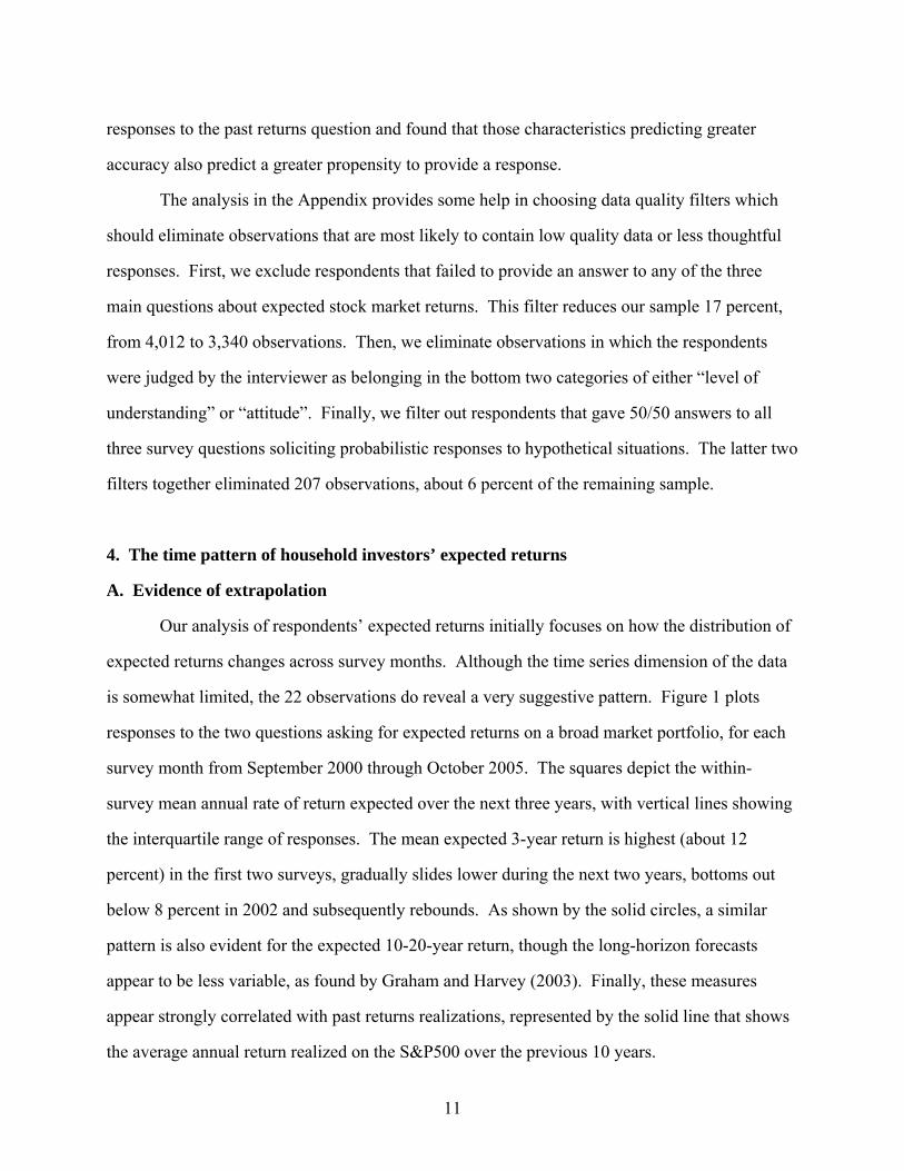
Our analysis of respondents’ expected returns initially focuses on how the distribution of

expected returns changes across survey months. Although the time series dimension of the data

is somewhat limited, the 22 observations do reveal a very suggestive pattern. Figure 1 plots

responses to the two questions asking for expected returns on a broad market portfolio, for each

survey month from September 2000 through October 2005. The squares depict the within-

survey mean annual rate of return expected over the next three years, with vertical lines showing

the interquartile range of responses. The mean expected 3-year return is highest (about 12

percent) in the first two surveys, gradually slides lower during the next two years, bottoms out

below 8 percent in 2002 and subsequently rebounds. As shown by the solid circles, a similar

pattern is also evident for the expected 10-20-year return, though the long-horizon forecasts

appear to be less variable, as found by Graham and Harvey (2003). Finally, these measures

appear strongly correlated with past returns realizations, represented by the solid line that shows

the average annual return realized on the S&P500 over the previous 10 years.

11

The effect of past returns on expected returns is further explored by regressions shown in

Table 2.14 Average past returns are persistent regressors, and there is some risk that this

relationship is at least partly spurious, as suggested by Boudoukh et.al. (2007). To mitigate such

concerns and to employ a unique aspect of our data, we augment the set of regressors with

respondent’s recollection of past returns. As shown in columns (1) and (4), both idiosyncratic

perceptions of past returns and actual past returns are highly influential in shaping respondents’

outlook over the medium- and long-run horizons. At the same time, past 3-month return has no

effect on expectations, suggesting that, while investors appear to predict continuation of multi-

year trends, they do not put extra weight on very recent fluctuations.

Qualitatively, these findings are consistent with previous survey-based studies of

expected stock returns. Fisher and Statman (2002) and Vissing-Jorgensen (2003) find a strong

positive relationship between recent performance and 12-month ahead expected returns,

measured in monthly UBS-Gallup surveys of mutual fund investors. DeBondt (1993) reports a

similar result for a sample of MBA students and mailed-in survey responses. In their study of

CFOs’ stock market expectations, Graham and Harvey (2003) find that recent returns (ranging

from one week to one quarter) have a strong positive effect on the one-year-ahead equity

premium, but not on the 10-year forecast.

B. Does wealth matter?

As pointed out by Campbell (2006), in the context of asset-pricing models, wealthy

households should have a disproportionate impact on equilibrium asset returns. Consequently,

we follow Vissing-Jorgensen (2003) in examining whether the time series pattern of

expectations, or the inclination to extrapolate from past returns, differs for respondents that have

more at stake in the equity market and thus have stronger incentives to be informed. To do so,

we divide the sample according to whether respondents had equity holdings in excess of

14 These regressions are estimated with the iterative GLS regression of Hamilton (1991) that applies progressively smaller weights to outliers in order to minimize their influence on the results. This algorithm is referred to as “robust regression” and is available as part of the standard Stata package.

12

$75,000, roughly the median reported equity wealth, and re-estimate the expected returns

regressions for the wealthier subsample. The estimated coefficients, reported in columns (2) and

(4), are quite similar to those based on the entire sample for both forecast horizons. As an

alternative, we estimate a weighted least squares specification, with weights being proportional

to the log of reported equity holdings. As shown in columns (3) and (6), this has no effect on the

results.15

In sum, wealthier investors have the same proclivity to extrapolate from past longer-term

returns as those with smaller stakes in the equity market. At first glance, this result seems to

contradict Vissing-Jorgensen (2003), which finds that wealthier investors are less prone to link

expected 12-month returns to their own portfolio returns over the prior 12 months. However, our

exercise differs in two respects. First, our regressions gauge the link between expected market

returns and past market returns (recalled and actual). In addition, we are focusing on somewhat

longer-horizon forecasts. Thus, even if wealthier investors are less prone to extrapolate year-

ahead market returns from their own recent performance (the biased self-attribution results in

Vissing-Jorgensen), their tendency to forecast persistence in market returns, over the medium- or

long-term, looks no different than that for the average investor.

5. Expected returns and macroeconomic conditions

The broad consensus interpretation of predictability in stock market returns, first

proposed by Fama and French (1989), presumes that conditioning variables are closely tied to

the business cycle. In this section, we examine the relationship between households’

expectations of economic conditions and their forecasts of stock returns.

A. Measuring economic expectations

While our special survey data are inadequate for conducting a definitive time series

analysis of expected returns and its relation to the business cycle, the Michigan Survey does

15 These results are robust to allowing median equity holdings thresholds vary by survey or restricting the sample to the top quartile.

13

solicit respondents’ views about current and prospective economic conditions. The resulting

cross-sectional variation facilitates an analysis of the relation between expected returns and

perceived economic conditions. We use the responses from three questions to construct three

measures of expected economic conditions – the first two are focused on the macroeconomy,

while the third relates to household income prospects.

Our primary measure of expected economic conditions is drawn from responses to the

following question:

“Looking ahead [is it more likely that the U.S. will have] continuous good times during the

next 5 years or so, or that we will have periods of widespread unemployment or depression,

or what?”

The answers are placed into five categories by the survey-giver: (i) bad times, (ii) bad times,

qualified (not good), (iii) pro-con, (iv) good times, qualified (not bad), or (v) good times. We

single out this question in particular because it focuses on real economic activity, rather than

“financial” conditions. The top panel of Table 3 summarizes the distribution of responses for

selected dates in our sample. Clearly, there are periods with a good deal of disagreement about

macroeconomic prospects. For instance, following the attacks of September 11, over 40 percent

of respondents expressed pessimism about future economic prospects, while the same share

expected continuously strong economic performance. In October 2005, in the wake of Hurricane

Katrina and soaring energy prices, more than half of the respondents were gloomy about the 5-

year outlook, but about a third were solidly optimistic.

The coded responses are used to construct an ordinal measure of the respondent’s

outlook, Good Times-5yrs, which takes integer values running from -2 (bad) to 2 (good).16 This

variable is thus interpreted as a measure of the perceived likelihood of a strong economy over the

next few years. Taken at face value, under the conventional interpretation of business cycle

conditionality, expected stock returns should be negatively related to Good Times-5yrs. In

16 Alternatively, we experimented with the use of dummy categories for the most optimistic and pessimistic households and found that this decomposition had no qualitative effect on results and their interpretation.

14

particular, investors are presumed to require – and expect – lower returns during good economic

times and higher returns during bad times.

Arguably, however, the heterogeneity in investor beliefs offers an alternative possible

interpretation of Good Times-5yrs that could justify a positive relation with expected stock

returns. Suppose respondents (rationally) associate a positive economic outlook with high

dividend growth and/or low stock return volatility. Then respondents who have a more favorable

outlook than the average investor (at any point in time) might rationally anticipate favorable

dividend surprises and/or a surprise drop in perceived risk that lowers required returns. In this

case, more optimistic respondents might expect such forthcoming news to cause the level of

stock prices to jump, which would boost returns over the period in question.

While it seems doubtful that most household investors would be confident enough in

their own views of the future state of the economy to predict an information effect on multi-year

returns, we try to address this possibility. In particular, we distinguish between the

“idiosyncratic” and “consensus” components of Good Times-5yrs by subtracting the survey-

specific mean response from the individual's response. The deviation from the average

respondent gauges the idiosyncratic component, whereas the average itself is interpreted as the

consensus view of the economy. Under the conventional hypothesis of countercyclical expected

returns, the level of the consensus outlook ought to be negatively related to expected returns,

while the idiosyncratic component could well have a positive effect.

We further attempt to control for expected changes in economic conditions using the

responses from a different survey question on economic expectations. That question asks:

“And how about a year from now, do you expect that … business conditions will be better or

worse than they are at present, or just about the same”

The responses are coded: worse, better, or the same. We quantify them with a single variable,

Better Conditions-12 mos, with a value of -2 (worse), 0 (same), or 2 (better). As a measure of

sentiment, Better Conditions-12 mo. differs from Good Times-5yrs in two ways that makes a

15

“news-surprise” interpretation somewhat more plausible.17 First, the question focuses on

change, which is more suggestive of a news interpretation. Second, it pertains to a short horizon,

for which it is more plausible that household investors have some conviction about their own

views of economic conditions.

The third and final measure of perceived economic conditions focuses on the

respondent’s expectations for their own economic prospects. It asks:

“What do you think the chances are that your (family) income will increase by more than the

rate of inflation in the next five years or so?”

The responses, and the associated variable (chances own income outpaces inflation), run from 0

to 100. If the first two proxies adequately control for respondents’ expectations of the

macroeconomy, then a rational investor’s response to this question would not have incremental

explanatory power for expected stock market returns (or risk). On the contrary, if this variable

does convey additional information on their views of the business cycle, then the presumption of

countercyclical stock returns would predict a negative relationship.

Correlations among the three measures of expected economic conditions, and their

correlations with expected returns, are shown in Panel B of Table 3. Not surprisingly, the three

measures are related. However, none of the correlations between the proxies exceeds 50 percent,

suggesting that each contains some independent information.

The bottom half of the table shows correlations between the measures of expected

economic conditions and expected stock returns, which foreshadow some of our main results.

The first number in each pair is the correlation in the pooled microdata, while the second

represents the correlation between the time-series of survey means. The latter could indicate

whether correlations are at least partly driven by variation in average views over time, rather than

just cross-sectional variation in optimism. As shown, each measure of expected conditions is

positively correlated with expected returns in the microdata, both at the 3-year and 10-year

17 Aside from the news-surprise interpretation of this variable, its predicted correlation with expected returns is ambiguous.

16

horizon. Moreover, in the case of Good times next 5-yrs, correlations with expected returns are

much higher in the time-series means, exceeding 0.66 at both forecast horizons. This suggests

that expected returns are strongly procyclical. In contrast, the time series correlations for Better

conditions-12 mo – our measure of expected news – are insignificant.

B. Regression results

In addition to these survey-based measures of expected economic conditions, the

expected return regressions include our measure of past actual returns (over a similar horizon)

and several controls for demographic characteristics, including age, education, gender, and years

of investment experience. Columns (1) and (4) of Table 4 present regression results for 3-year

and 10-year expected returns, respectively. To minimize the influence of outliers, these

regressions are estimated using Hamilton’s (1991) “robust regression” algorithm.18

As shown by the first two coefficient estimates, both measures of expected

macroeconomic conditions have positive and statistically significant effects on expected returns

over both horizons. We note in particular the positive coefficient on Good Times-5yrs, which is

interpreted as indicating that expected returns are “procyclical”: expectations of better economic

performance are associated with higher expected stock market returns.19 The difference in

expected 3-year returns between optimistic and pessimistic respondents is about 1 percentage

point (0.28*4). Although not shown, we find virtually identical coefficients when regressions

are estimated on the subsample of respondents with greater than average stock market wealth.

Similarly, investors’ expectations of their own income prospects have a consistently

positive effect on their stock market outlook. The magnitude and the statistical precision of this

effect are about the same for the two horizons. A coefficient of 0.012 implies that investors with

18 This procedure is defined in footnote 12. Alternative approaches included quantile (median) regression or truncation of the top and bottom percentile responses in each survey with subsequent OLS estimation, both of which produced results that are qualitatively similar to robust regression. 19 The regressions in Table 4 get much (but not all) identification from cross-sectional variation in beliefs about future business conditions and disagreement on where the economy is now. Hence, "procyclical" should be taken to mean not just the usual "as the business cycle evolves", but also "as the business cycle is perceived by respondents".

17

responses at the top of the interquartile range (75 percent chance of real income growth) expect

the market to return 0.6 percentage points more than respondents at the bottom of the range (20

percent chance). Taken at face value, this result suggests that investors’ views about their own

income prospects distort their expectations for market returns. However, this variable could also

contain information about macroeconomic expectations not captured by the first two variables.

As suggested earlier, our measure of macroeconomic conditions (Good Times-5 yrs)

might also serve as an indicator of the news that respondents believe the market will learn over

time. This caveat is addressed in columns (2-3) and (5-6) of Table 4, which show regression

results when Good Times-5yrs is decomposed into an idiosyncratic (expected news) component,

Good Times-5yrs Deviation, and a consensus component, Good Times-5yrs Mean. Not

surprisingly, the coefficient on the idiosyncratic component of expected economic conditions

remains positive and significant in each case. The more interesting result is that the coefficient

estimate on Good Times-5 yrs Mean is also consistently positive; in fact, in all specifications it is

larger than the coefficient on the idiosyncratic component.20 Thus, household investors expect

higher returns when the consensus expectation calls for economic expansion.

Another interesting finding, shown in columns (3) and (6), is that excluding past returns

from the regression boosts the coefficients on Good Times-5yrs Mean. This reflects a strong

positive correlation between past returns and the consensus forecast of economic conditions.

Hence, extrapolation from past returns may derive in part from expectations of persistence in

economic conditions, together with an association of good (bad) conditions with high (low)

returns. In any case, the regression results appear to contradict the standard view on the

cyclicality of expected returns.21 20 Standardized coefficients (not shown) also imply that the magnitude of the consensus effect is greater than that of the idiosyncratic component. For example, a one standard deviation shock to Good Times - Mean results in medium-term expected returns that are 0.72 percentage points higher, while a similar shock to Good Times – Deviation increases expected returns by 0.47 percentage points. 21 As an aside, these findings suggest a potential rationalization of the high historical average equity premium. As argued by Shefrin (2005, p. 436), if investors overestimate the positive relation between the stocks and the economy, as household investors appear to do in our data, then they probably overestimate the covariance between equity returns and consumption. If so, then they will tend to underweight equities and boost required returns.

18

These conclusions are insensitive to the choice of demographic controls, most of which

have little explanatory power. In fact, gender is the only such characteristic with a substantial

and highly significant effect on expected returns, though only for the shorter horizon. Perhaps

more surprising is the finding that investor experience and age do not influence expected returns.

This contrasts with Vissing-Jorgensen (2003), where more experienced and older investors in the

Gallup/UBS polls were consistently found to be less optimistic about both 1- and 10-year

expected returns over the 1998-2002 period. As we shall see below, demographic characteristics

play a much larger role in determining investor perceptions of uncertainty.22

6. Determinants of perceived risk

As described earlier, our measure of perceived risk is constructed from respondents’

assessments of the likelihood that market returns will fall outside the 4 percentage point band

centered on their long-term return forecast. We label this probability measure “Uncertainty”,

and interpret higher values as indicating higher perceived return volatility. 23

A. Economic outlook and demographic characteristics

Of primary interest is the relationship between perceived risk and expected business

conditions. The research on time-varying volatility, while not conclusive, leans toward the view

that conditional volatility in stock market returns is countercyclical (see, for example Schwert,

1989 and Hamilton and Lin, 1996). Most recently, Brandt and Kang (2004), using a latent VAR

approach on data from 1946-98, infer that “whenever the economy comes off the peak of a cycle,

the conditional volatility rises immediately” (p. 220).

22 When we allow for time-varying experience (and age) effects, we still fail to detect a moderating influence of experience on market expectations in our earlier surveys. 23 Throughout, we interpret investor responses to this survey question as primarily gauging perceived volatility of stock market returns. However, we recognize that replies may well conflate notions of uncertainty and risk, with some interpreting the question as a referendum on their forecasting ability, rather than a question about objective risk in the stocks. If so, higher numeric responses to this question could be indicative of overconfidence in the operational sense of Gervais and Odean (2001) or Graham and Harvey (2007). The relative importance of these two interpretations presents a difficult and interesting question, which is left for future research.

19

To gauge how perceptions of risk change with business cycle conditions, we regress

Uncertainty on the measures of expected macroeconomic conditions analyzed in the previous

section. 24 These regressions also control for the potential influence of several demographic

factors and survey fixed effects. As shown in the Column 1 of Table 5, the coefficient on Good

times-5 yrs is negative and significant, implying that respondents expecting favorable economic

conditions over the next few years are less uncertain about longer-run equity returns. On the

other hand, the expected near-term change in conditions, Better conditions-12 mos., has no

marginal effect on Uncertainty, a result that seems quite reasonable given the mismatch in

horizons.

Finally, the respondent’s belief that their own household income is more likely to outpace

inflation has a significant negative effect on Uncertainty. This finding can be interpreted as

implying that investors’ own personal economic security distorts their perceptions of stock

market risk. Alternatively, this variable might serve as an additional proxy for expected

macroeconomic growth, which has a negative effect on perceived risk.

In contrast with the earlier findings on expected returns, it appears that Uncertainty is

also influenced by several demographic characteristics. Gender, the only such characteristic that

mattered for expected return, also influences perceived risk: males tend to report substantially

lower Uncertainty. But we also find that Uncertainty is negatively related to higher education

and years of investment experience – characteristics that are all presumably correlated with the

respondent’s level of financial market knowledge. These results suggest that Uncertainty

contains an element of subjective uncertainty in addition to perceived objective risk. In other

words, increased knowledge due to education or experience boosts the respondent’s confidence

in their own forecast, which induces a tighter subjective distribution for expected returns.

24 We use raw probability responses instead of imputed standard deviations on the left-hand side to minimize sample attrition stemming from purely mechanical imputation problems discussed earlier. This also allows the analysis to be robust to other return distributions, since the relationship between a covariate and a raw probability response will have the same sign as that between a covariate and an implied standard deviation for any underlying distribution.

20

The negative coefficient on Good times-5 yrs, while consistent with the view that stock

market volatility is countercyclical, poses a conundrum when viewed in conjunction with our

finding of procyclical expected returns. Specifically, it implies that respondents associate

economic expansion or its likelihood with both high expected returns and low risk, while the

prospect of poor economic conditions is associated with both lower expected returns and higher

risk. Taken at face value, these results imply that forward-looking Sharpe ratios of household

investors are procyclical, which presents obvious problems for rational asset pricing models.

That is, equity risk premiums do not appear to compensate for these investors’ exposure to

macroeconomic risks.

Indeed, we can construct estimates of household-level Sharpe ratios for the broad equity

market using the implied standard deviation of returns backed out from Uncertainty (Table 1),

together with 3-year or 10-year expected returns and Treasury bond yields of matching horizons.

When these Sharpe ratios are regressed on our measures of expected economic conditions and

other covariates, as in Tables 4 and 5, we indeed find them to be generally positively related to

respondents’ economic outlook. For the 3-year horizon, both the consensus and idiosyncratic

macroeconomic expectations (Good Times 5 yrs) have significant positive effects on Sharpe

ratios. For the 10-year horizon, the consensus expectation has no effect, while idiosyncratic

views remain strongly positive, mirroring the pattern of results for expected returns in Table 4.

In any case, however, there is no evidence of countercyclicality in forward-looking Sharpe ratios.

B. Representativeness heuristic

While the apparent procyclical pattern of Sharpe ratios is difficult to reconcile with

finance theory, the result does accord with some recent research on cognitive biases in financial

decision-making.25 In particular, the pairing of higher expected return with lower risk and a

stronger economy is consistent with what behavioral theorists have labeled the

25 The study of systematic deviations in human thought processes from rational precepts, which has a rich history in social and cognitive psychology, has become increasingly influential in financial economics (see Hirshleifer (2001) and Barberis and Thaler (2003) for a review).

21

representativeness heuristic (Tversky and Kahneman, 1974). An investor influenced by this

heuristic tends to assess the probability of an event by the degree to which it: (i) is

“representative” of the available evidence; and (ii) reflects the salient features of the process by

which it is generated. Here, the widespread expectation of a good economy apparently boosts

prospects for a “good” stock market, that is, high expected returns and low risk.

Indeed, this “good-good” association between the economy and stock returns is

analogous to the finding by Shefrin and Statman (1995) that investors expect higher returns from

those stocks they also view as safer. They suggest that this positive association is a result of a

potentially inappropriate linking of characteristics that appear salient in some cognitive sense. If

low risk and high returns are each associated with a “good” company, this cognitive bias can

lead an investor to believe that the stock of a “good” company will have low risk and high

expected return.

Our survey data allow a more direct test of the role of the representativeness heuristic. In

particular, we can measure the “representativeness” of respondents’ 10-year return forecasts by

comparing those forecasts with the respondent’s recalled past 10-year return on the S&P 500 –

the “available evidence” that influences their outlook. We measure “representativeness” as the

absolute value of the difference between their longer-term forecast and their recollection of

historical returns. The representativeness hypothesis predicts that, when this discrepancy is

larger, the respondent will be less confident in their expected return forecast and, thus, will tend

to assign a lower probability of realizing a return that is close to their forecast -- Uncertainty will

be higher. Column (2) shows regression results when our measure of representativeness in

included. The positive coefficient on the discrepancy between expected returns and recalled past

returns is highly significant and economically sizable, which we interpret as evidence for the

representativeness heuristic.

As a test of robustness, we re-estimate (2) on a subsample that excludes investors with

reported Uncertainty values of 50 percent. As noted earlier, some of those respondents may

simply have no opinion to the question, in which case their responses would weaken the

22

estimated relationships. The results in column (3) are consistent with this interpretation. The

estimated coefficients on nearly all the variables increase in magnitude; moreover, they retain

statistical significance despite the drop in sample size. Finally, in both (2) and (3), the addition

of behavioral controls does not eliminate the estimated inverse relationship between Uncertainty

and expected (longer-term) business conditions, as reflected in Good Times-5 yrs.

7. Do investors' actions reflect beliefs?

The relevance of our inferences about investor beliefs hinges on whether those beliefs, as

measured in our data, actually influence portfolio allocation decisions. This section examines

evidence of a relationship using data on respondents’ reported portfolio equity allocations

(described in section 2.B). The most succinct test of the value-relevance of reported beliefs

involves comparing (expected) Sharpe ratios across respondents reporting different portfolio

exposures to equities. Here, Sharpe ratios are measured using expected 10-year returns on

respondents’ own equity portfolios divided by the implied standard deviation of returns on the

broad market. As shown in Table 6, there is a monotonic upward progression in median (and

mean) Sharpe ratio as we move from respondents in the lowest equity portfolio share bucket to

those in the highest bucket. Moreover, differences in the median Sharpe ratios between

households with low (less than 25 percent), middle (between 25 and 50 percent), and high (more

than 75 percent) equity exposures are all statistically significant.

To test whether both factors that comprise the Sharpe ratio have explanatory power for

portfolio holdings, we estimate a regression motivated by the classic portfolio choice model of

Samuelson (1969). That model implies that the portfolio share invested in stocks should be

proportional to the expected risk premium and inversely proportional to expected variance times

the coefficient of relative risk aversion: sharei = (Rie – Rf) / γi E[Vari(R)]. Taking logs on both

sides yields a linear regression specification:

log (sharei) = β 0 + β1 log (Rie – Rf) + β2 log (E[Vari(R)]) + εi , (1)

23

Here, share is measured as the midpoint of the porfolio equity share buckets and Rf is measured

by the yield on the 10-year Treasury bond at the time of survey. Because risk aversion is

unobservable, the idiosyncratic component of risk aversion is in the regression error term, while

the average level of risk aversion is reflected in the constant. Finally, to control for life-cycle

effects abstracted from in this static model, regressions also include age-group dummies. To

check the robustness of our results to the log transformation implied by (1), we also estimate a

reduced form linear specification, where portfolio share is regressed on expected excess return,

Rie – Rf, and Uncertainty.

After removing observations with values of the two key explanatory variables in the

extreme 2 percentiles, we estimate the log-log specification (1) using OLS.26 The results are

reported in the bottom panel of Table 6. The estimated coefficients on both expected returns and

perceived risk are statistically significant and their signs are consistent with theory: equity

portfolio shares are increasing with expected (excess) returns and decreasing with expected risk.

One disadvantage of the log-log transformation is that the log of excess expected return is

undefined for observations in which excess return is negative. To avoid losing those

observations, we estimate a modified version of (1) in which the first term is simply the log of

expected stock returns. Here, time dummies implicitly control for time-variation in the risk-free

rate. As shown in the panel’s second column, both coefficients are again significant – with that

on the log expected return being larger – and the R-squared is a touch higher.

While these results are statistically strong, one might be concerned that the coefficients

are so small compared to the predictions of the theoretical model. One reason could be the very

coarse measure of equity portfolio share, the dependent variable. For example, investors with

equity shares of 26 and 45 percent are observationally equivalent in our data. Another likely

factor is measurement error in our expectations variables (particularly perceived risk), which

26 Since our dependent variable is discrete and follows a clear ordinal ranking, we also estimated the reduced-form version using ordered logit, which produced qualitatively similar results. As the OLS estimator is consistent and is easier to interpret, we focus on the least-squares results.

24

could cause attenuation bias that pushes both β’s towards zero. To address this concern, we also

estimate an IV specification (not shown) in which expected volatility and excess returns are

instrumented by their respective ranks.27 In this variant, the coefficient on instrumented

volatility variable rises to -0.13, while that on expected excess returns is virtually unchanged.

Finally, a more conceptual explanation is the static nature of the model (1). In a dynamic

framework, portfolio sensitivity to expectations might be muted by transaction costs and inertia

or inattention that inhibits rebalancing in response to a shift in expectations.

To check the robustness of these results, we also estimate a reduced-form linear

specification (column 3), in which portfolio share is regressed on expected excess return, Rie –

Rf, and Uncertainty. Here again, the coefficients have the expected signs and are statistically

significant. Finally, as a nod toward potential dynamic effects, we augment the set of regressors

with a measure of the duration of investor experience. As shown in column 4, the coefficients on

the fundamentals are unaffected, but we find that the duration of investor participation in the

stock market itself has a strong positive effect on portfolio share. One possible explanation for

this could be investor inertia: those with longer market tenure built up more equity wealth during

the bull market of the 1980s and 1990s. If investors do not optimally rebalance their portfolios

but rather tend to “let winnings ride,” then more years of experience would have induced higher

current portfolio equity shares.

Regardless of specification, the portfolio regressions provide consistent evidence that

survey responses to questions about expected risk and return reflect the actionable views of

respondents, and not just idle speculation. This provides additional credibility to our seemingly

anomalous finding of procyclical Sharpe ratios.

8. Reconciliation with return predictability literature

27 The assumption here is that the ranking of expected volatility is driven by the true measure of risk perception and not by the measurement error.

25

As emphasized earlier, the apparent pro-cyclicality of household investor expected equity

returns appears to contradict the conventional interpretation drawn from the literature on return

predictability. In those studies, the measure of expected return is actual return, while economic

conditions are measured by macroeconomic variables such as financial ratios. Thus, our finding

is drawn from regressions in which the dependent variable, expected stock returns, as well as our

proxies for the business cycle, all differ from those in the return predictability literature.

To clarify the source of the disagreement, it would be useful to correlate our survey-

based measure of expected returns with some of the more conventional conditioning variables.

The main obstacle to such an exercise is the very limited time series of our expected return

measures; but this shortcoming can be overcome somewhat by using another source of

household investor expected returns – the Gallup/UBS poll of mutual fund investors (analyzed in

Vissing-Jorgensen, 2003). Each monthly Gallup/UBS survey consists of interviews with roughly

1,000 respondents that have at least $10,000 in mutual fund holdings. Monthly summary

statistics are available beginning in June 1998 and, where they overlap, mean Gallup/UBS

responses match up quite well with the Michigan survey means.

Figure 2 shows a comparison of mean responses from two Gallup/UBS questions against

the mean expected 3-year annual rate of return from our survey. The Gallup/UBS survey asks

investors for expected returns, over the next 12 months, on (i) their own investment portfolios

(the solid line) and (ii) the stock market (the dashed line). The means of the two series are highly

correlated over time (ρ=0.97), though expected own-portfolio returns are nearly always a bit

higher than expected market returns. Each series, in turn, is closely correlated with the monthly

mean responses from the Michigan survey (the dots), despite the somewhat different horizons.

For overlapping survey months, that correlation exceeds 85 percent. In the analysis here, we

focus on the longer of the two Gallup series – own portfolio return expectations.

Arguably, two of the most important conditioning variables in the predictability literature

are the dividend yield and CAY, the log of the consumption-wealth ratio. The dividend yield has

received the most attention historically, although the robustness of its predictive power has been

26

the subject of some debate (Stambaugh, 1999)28. CAY was introduced relatively recently by

Lettau and Ludvigson (2001), but its predictive power is relatively large and its statistical

significance well documented. Both of these variables have been shown to be positive predictors

of actual quarterly, annual and long-horizon stock returns; thus, they are normally interpreted as

positive indicators of (rational) cyclical variation in expected returns. For instance, Lettau and

Ludvigson (2001, p. 817), argue that CAY predicts asset returns because “when excess returns

are expected to be higher, forward-looking investors will react by … allowing consumption to

rise above its common trend” with current asset wealth.

However, as shown in Figure 3, the correlation between expected returns, as measured in

the surveys, with both CAY (panel A) and the S&P 500 dividend yield (panel B) is strongly

negative over this sample period. This suggests that conditional expected returns, inferred from

regressions of realized returns on the dividend yield or CAY, are extremely poor – in fact,

contrary – measures of household investor expectations. This is not because the surveyed

individuals have little market relevance. As we have shown, the time series behavior of our

survey-based expected returns is practically identical when the sample is constructed using only

those households with a substantial stake in the market (more than $75,000 in equities).

One potential rationalization for the contradiction is that the dividend yield and CAY do

not have the traditional positive conditioning effect on realized returns in our limited (and very

recent) sample period. To check this, we estimate simple regressions of annual real returns on

the dividend yield and CAY in the 1998-2006 sample at the quarterly frequency. In our short

sample, we still obtain a significantly positive coefficient on the dividend yield of 1.55, even

larger than in commonly-used sample periods. Separately, we find that the coefficient on CAY

28 The statistical significance of the dividend yield is not entirely robust to sample period in that literature, but Boudoukh, et al. (2007) find that this owes to the rising importance of stock repurchases as a payout tool between 1984 and the mid-1990s.

27

for the 1998-2006 sample is not quite significant (p-value of 0.14); however, at 4.6, it is also

positive and qualitatively the same as in long-sample regressions.29

Thus, to argue that the conventional approach to gauging time-varying expected returns

produces a reasonable measure of the “market expectation,” one must argue (i) that institutional

investors (aside from mutual funds) have polar opposite beliefs to those of households and (ii)

that those institutional investors are far more influential in asset price determination. If either of

these conditions fails to hold, then the contradictory inferences are reconciled in a scenario like

the following: households associate a favorable macroeconomic outlook with high and less

volatile stock returns. They act on these expectations by shifting assets into equities, driving up

equity prices, which also drives down the dividend yield. At such times, household investors

must on average have unduly optimistic expectations; thus, going forward, the “inflated” stock

valuations create the conditions for low realized returns.

9. Conclusion

Using data obtained from a series of Michigan Surveys of Consumer Attitudes, we

examine the stock market beliefs of household investors – an important subset of market

participants by the sheer proportion of outstanding equities they hold. In forming expectations of

future returns, household investors appear to extrapolate from recent-years’ realized returns.

While this is generally consistent with the findings of previous survey-based studies, our survey

results indicate that this tendency is equally strong among wealthy and less wealthy households.

Another key, and apparently somewhat related, finding is that expected returns appear to

be procyclical. When investors report more optimistic assessments of macroeconomic

conditions for the coming years, they also tend to expect higher returns over similar periods.

This contrasts sharply with inferences normally drawn from the conventional approach of

29 When estimated on the post-war data, the coefficient on the dividend yield in such regressions is traditionally found to be around 0.33 (Campbell, Lo, MacKinlay, p.269), while the coefficient on CAY reported by Lettau and Ludvigson (2001) ranges between 4 and 5.

28

regressing realized returns on conditioning variables. In addition, we find that perceived risk, or

uncertainty, is lower when favorable economic conditions are expected. Together these results

imply that forward-looking Sharpe ratios are procyclical, a seeming contradiction of the

predictions of rational asset-pricing models.

The credibility of these findings is bolstered by robustness of the cross-sectional

estimates, the ability to control for response quality and, perhaps most of all, and by the finding

that respondents’ equity exposures are consistent with their reported beliefs. Specifically, equity

exposures tend to increase with self-reported expected returns and decline with perceived

uncertainty. All told, these results lend support to a behavioral explanation for time-varying

stock returns. In particular, equity valuations are lower during recessions – and subsequent

returns are higher – because at those times individual investors are pessimistic about future stock

market performance.

Of course, the rejoinder to this conclusion is that professional investors are likely to be

much more rational; therefore, they could take positions that counter the influence of household

investors. While this is plausible, it is not at all clear that rational investors as a group would or

could entirely offset systematical irrational trading by household investors. Not only do they

have limited capital, but many of them might see greater profitability in trying to “ride the

bubble” (Brunnermeier and Nagel, 2004, Hofsinger and Sias, 1999). The final verdict on the

importance of household investor beliefs thus rests with the identity of the “marginal investor”, a

subject that lies beyond the scope of this paper.

29

References John Ameriks and Stephen P. Zeldes, “How do household portfolio shares vary with age?”

mimeo 2001. Brad M. Barber and Terrance Odean, “Boys will be boys: Gender, overconfidence, and common

stock investment,” Quarterly Journal of Economics, 116(1), 2001. Nicholas Barberis, Andrei Shleifer, and Robert Vishny, “A model of investor sentiment,”

Journal of Financial Economics, 49(3):307–343, 1998. Nicholas Barberis and Richard Thaler, “A survey of behavioral finance,” vol 1b in Handbooks in

Economics, chapter 18, 1st edition, Elsevier North-Holland, 2003. Itzhak Ben-David, John Graham and Campbell Harvey, “Managerial overconfidence and

corporate policies,” mimeo, September 2007. Sylvia Beyer, “Gender differences in the accuracy of self-evaluations of performance,” Journal

of Personality and Social Psychology, 59:960–970, 1990. Jacob Boudoukh, Roni Michaely, Matthew Richardson, and Michael R. Roberts, “On the

importance of measuring payout yield: Implications for empirical asset pricing,” Journal of Finance, 62(2):877:915, 2007.

Wandi Bruine de Bruin, Paul S. Fischbeck, Neil A Stiber, and Baruch Fischhoff, “What Number is “Fifty-Fifty”?: Redistributing Excessive 50% Responses in Elicited Probabilities,” Risk Analysis, 22(4):713-723, 2002.

Markus K. Brunnermeier and Stefan Nagel, “Hedge Funds and the Technology Bubble,” Journal of Finance, 59(5):2013-2040, 2004.

Markus K. Brunnermeier and Stefan Nagel, “Do Wealth Fluctuations Generate Time-varying Risk Aversion? Micro-Evidence on Individuals' Asset Allocation,” mimeo, Princeton University, 2006

John Y. Campbell and John H. Cochrane, “By force of habit: A consumption based explanation of aggregate stock market behavior,” Journal of Political Economy, 107(2):205–251, 1999.

John Y. Campbell, Andrew Lo, and Craig MacKinlay. The Econometrics of Financial Markets (Princeton University Press, Princeton, NJ), 1997.

Murillo Campello, Long Chen, and Lu Zhang, “Expected Returns, Yield Spreads, and Asset Pricing Tests,” mimeo, University of Illinois-Champaign, January 2003.

Nai-Fu Chen, Richard Roll, and Stephen A. Ross, “Economic Forces and the Stock Market” Journal of Business, 59(3):383-403, July 1986.

James Claus and Jacob Thomas, “Equity Premia as Low as Three Percent? Evidence from Analysts' Earnings Forecasts for Domestic and International Stock Markets,” Journal of Finance, v. 56(5):1629-66, October 2001.

John H. Cochrane, “Where is the market going? Uncertain facts and novel theories,” Economic Perspectives, 21(6), 1997.

Kent Daniel, David Hirshleifer, Avanidhar Subrahmanyam, ”Investor Psychology and Security Market Under- and Overreactions,” Journal of Finance, 53(6):1839-85, December 1998.

30

Jeff Dominitz and Charles F. Manski, “How Should We Measure Consumer Confidence? Journal of Economic Perspectives, 18(2): pp. 51-66, Spring 2004.

Jeff Dominitz and Charles F. Manski, “Measuring and Interpreting Expectations of Equity Returns,” mimeo, Northwestern University, June 2005.

Karen E. Dynan, “Habit formation in consumer preferences: Evidence from panel data”, American Economic Review, 90(3):391–406, 2000.

Edwin J. Elton, “Expected Return, Realized Return, and Asset Pricing Tests,” Journal of Finance, 54(4):1199–1220, August 1999.

Robert Engle, “Risk and Volatility: Econometric Models and Financial Practice”, Nobel Memorial Lecture, 2003.

Eugene F. Fama and Kenneth R. French, “Business conditions and expected returns on stocks and bonds,” Journal of Financial Economics, 25(1):23–49, November 1989

Eugene F. Fama and Kenneth R. French, “The equity premium,” Journal of Finance, 57(2):637–59, April 2002.

Kenneth L. Fisher and Meir Statman, “Blowing Bubbles,” Journal of Psychology and Financial Markets, 3(1): 53-65, 2002.

Kenneth L. Fisher and Meir Statman, “Consumer Confidence and Stock Returns,” Journal of Portfolio Management, 115-27, Fall 2003.

William Gebhardt, Charles Lee, and Bhaskaran Swaminathan, “Toward an Implied Cost of Capital,” Journal of Accounting Research, v. 39(1):135-76, June 2001.

Simon Gervais and Terrance Odean, “Learning to be overconfident,” Review of Financial Studies, 14(1):1–27, Spring 2001.

Markus Glaser, Thomas Langer, Jens Reynders and Martin Weber, “Framing Effects in Stock Market Forecasts: The Difference Between Asking for Prices and Asking for Returns,” Review of Finance, 11: 325:357, April 2007.

Amit Goyal and Ivo Welch, “Predicting the Equity Premium With Dividend Ratios,” National Bureau of Economic Research Working Paper No. 8788, 2002.

John R. Graham and Campbell R. Harvey, “Market timing ability and volatility implied in investment newsletters’ asset allocation recommendations,” Journal of Financial Economics, 42(3):397–421, 1 November 1996.

John Graham and Campbell Harvey, “Expectations of equity risk premia, volatility and asymmetry from a corporate finance perspective,” working paper, Duke University, 2003.

John Graham and Campbell Harvey, “The long-run equity-risk premium,” Finance Research Letters 2: 185-194, 2005.

James D. Hamilton and Gang Lin, “Stock market volatility and the business cycle”, Journal of Applied Econometrics, 11(5): 573-593, September-October 1996.

Lawrence Hamilton, “srd1: How robust is robust regression?” Stata Technical Bulletin 2:21-26. Lars Peter Hansen and Kenneth J. Singleton, “Stochastic consumption, risk aversion, and the

temporal behavior of asset returns,” Journal of Political Economy, 91:249–265, April 1983.

Lars Peter Hansen and Thomas J. Sargent, “Acknowledging misspecification in macroeconomic theory”, Review of Economic Dynamics, 4(3):519-35, July 2001.

31

David Hirshleifer, “Investor psychology and asset pricing,” Journal of Finance, 56(4):1533-97, August 2001.

Lee, Charles, Andrei Shleifer, and Richard Thaler, “Investor Sentiment and the Closed-End Fund Puzzle”, Journal of Finance, 46:75-109, March 1991.

Martin Lettau and Sydney Ludvigson, “Consumption, Aggregate Wealth, and Expected Stock Returns,” Journal of Finance, 56(3):815-49, June 2001.

Joseph P. Lupton, “Household portfolio choice and habit liability: evidence from panel data”, working paper, Federeal Reserve Board, 2003.

Daniel Kahneman and Amos Tversky, “Prospect theory: An analysis of decisions under risk,” Econometrica, 47:263–291, March 1979.

Robert C. Merton, “Lifetime portfolio selection under uncertainty: The continuous time case,” Review of Economics and Statistics, 51(3):373–413, 1969.

John R. Nofsinger and Richard W. Sias, “Herding and Feedback Trading by Institutional and Individual Investors,” Journal of Finance 54 (6), 2263-2295.

Terrance Odean, “Volume, volatility, price and profit when all traders are above average,” Journal of Finance, 53(6):1887–1934, December 1998.

Lily Qiu and IvoWelch, “Investor Sentiment Measures”, working paper, July 2006 Enrichetta Ravina, “Habit formation and keeping up with the Joneses: evidence from micro

data,” working paper, Northwestern University, 2005. Paul A. Samuelson, “Lifetime portfolio selection by dynamic stochastic programming,” Review

of Economics and Statistics, 51(3):239–246, 1969. G. William Schwert, “Why does stock market volatility change over time?,” Journal of Finance,

44(5): 1115-1153, December 1989. Hersh Shefrin, “Do investors expect higher returns from safer stocks than from riskier stocks?”

The Journal of Psychology and Financial Markets, 2(4):176–181, 2001. Hersh Shefrin, A Behavioral Approach to Asset Pricing (Elsevier Academic Press, Burlington

MA), 2005. Hersh Shefrin and Meir Statman, “Making sense of beta, size and book-to-market,” The Journal

of Porfolio Management, 22(2):22-26, 1995. Robert Shiller, “Measuring bubble expectations and investor confidence,” The Journal of

Psychology and Financial Markets, 1(1):49–60, 2000. Robert Stambaugh, “Predictive regressions,” Journal of Financial Economics 54, 375–421,

1999. Amos Tversky and Daniel Kahneman, “Judgment under uncertainty: Heuristics and biases,”

Science, 185(4157):1124–1131, 1974. Annette Vissing-Jorgensen, “Perspectives on behavioral finance: Does irrationality disappear

with wealth? Evidence from expectations and actions,” NBER Macroeconomics Annual, June 2003.

Welch, Ivo, “Views of Financial Economists on the Equity Premium and on Professional Controversies,” Journal of Business 73(4):501-537, October 2000.

World Bank, World Development Indicators, http://devdata.worldbank.org/query/default.htm, 2007

32

33

Appendix: Some tests of survey response quality

We can gauge the extent of survey respondents’ general knowledge about the stock

market by comparing their recollection of average returns over the preceding ten-year period

with actual historical return values.30 The results of this comparison are summarized in Figure

B.1, which plots the distribution of respondents’ recalled values (means and interquartile ranges)

along with the actual realized returns (geometric average of returns over the previous 10 years).

The results are plotted in calendar time, highlighting the irregularity of survey intervals.

The historical returns series reflect the extraordinary run up in equity prices in the late 1990’s

and their subsequent decline. The mean and the interquartile range of investors’ recalled market

return generally mimic the path of realized returns, although they display a more limited range of

movement. In particular, most respondents substantially underestimated the past 10-year returns

in the early surveys, perhaps reflecting a tendency to provide answers weighted toward

perceptions of longer-run experience.

Next, we examine whether absolute magnitudes of recall errors are systematically related

to respondent characteristics. In addition to demographic and stock ownership characteristics,

we considered two measures of response quality constructed from the survey interviewers’ coded

assessments of a respondent’s “level of understanding” (ranging from “excellent” to “poor”) and

“attitude” (ranging from “friendly and interested” to “hostile”). The results, available upon

request, generally suggest that the accuracy of a respondent’s recall of past returns improves

substantially with the size of their equity portfolio and education. The errors are also lower for

those who identify themselves as primary investment decision-makers, as well as for those whom

the questioner reported as having an excellent or good understanding of the survey question.

Finally, we consider the minority of respondents (13 percent) who declined to provide an

estimate of past returns. We find that many of the characteristics that predict greater recall errors

(i.e. lower-quality responses) also indicate a higher likelihood of declining to answer altogether.

30 The survey question read: “thinking about a diversified portfolio of stocks, what would you guess was the average annual return earned over the past 10 years?” This question was asked on surveys spanning the period from September 2000 through January 2003 and then again on October 2004 through October 2005 surveys.

Figure 1

Expected Returns vs. Past Returns

4

6

8

10

12

14

16

18

20

Jul Oct Jan Apr Jul Oct Jan Apr Jul Oct Jan Apr Jul Oct Jan Apr Jul Oct Jan Apr Jul Oct

Perc

ent R

etur

n

Expected, 10-20 yrs Expected, 3yrs Actual past 10-yr returns

2000 2001 2002 2003 20052004

The mean expected long-term and medium-term return among Michigan survey respondents each period are plotted (by the squares and circles); the vertical bars show the interquartile range of the responses. The line plots the realized average annual returns on the S&P500 over the 120-months preceding the survey date.

Figure 2 Measures of Expected Near-term Stock Market Performance

Michigan and Gallup Survey Means

4

6

8

10

12

14

16

18

20

Feb May Aug Nov Feb May Aug Nov Feb May Aug Nov Feb May Aug Nov Feb May Aug Nov Feb May Aug Nov Feb May Aug Nov Feb May Aug Nov

Ret

urn,

Per

cent

Gallup/UBS 12-month own return Gallup/UBS 12-month market return

Michigan 3-year market return

1999 2000 2001 2002 200620052003 2004

Expected 3-year market returns are survey-specific means of the Michigan survey respondents. The Gallup 12-month expected returns series are mean responses from monthly surveys jointly sponsored by the Gallup Organization and UBS. The dotted line depicts mean responses to the question on expected market returns, which was discontinued in May 2003. The solid line shows the (monthly) mean expected own portfolio return.

Figure 3 Survey Expected Returns and Conventional Macro Conditioning Variables

Panel A. CAY and Survey Expected Returns

4

6

8

10

12

14

16

18

20

Feb May Aug Nov Feb May Aug Nov Feb May Aug Nov Feb May Aug Nov Feb May Aug Nov Feb May Aug Nov Feb May Aug Nov Feb May Aug Nov

-4.0%-3.5%-3.0%-2.5%-2.0%-1.5%-1.0%-0.5%0.0%0.5%1.0%1.5%

Mean expected 12-month returns, Gallup/UBS (left axis) CAY deviation (right axis)

20012000 2003 2004 200520021999 2006

Panel B. Dividend yield and survey expected returns

4

6

8

10

12

14

16

18

20

Feb May Aug Nov Feb May Aug Nov Feb May Aug Nov Feb May Aug Nov Feb May Aug Nov Feb May Aug Nov Feb May Aug Nov Feb May Aug Nov

-4.6

-4.5

-4.4

-4.3

-4.2

-4.1

-4.0

-3.9

Mean expected 12-month returns, Gallup/UBS (left axis) ln S&P dividend yield (right axis)

20012000 2003 2004 200520021999 2006

Figure B.1 Actual vs. Recalled Average Stock Market Returns, Previous 10 yrs

4

6

8

10

12

14

16

18

20

Jul Oct Jan Apr Jul Oct Jan Apr Jul Oct Jan Apr Jul Oct Jan Apr Jul Oct Jan Apr Jul Oct

aver

age

annu

al re

turn

ove

r the

pas

t 10-

year

per

iod

Actual past returns Recalled past returns, mean and interquartile range

2000 20022001 200520042003

Actual stock market returns are defined as a geometric average of annual total returns on the S&P500 (total returns index) over the 120-month (10-year) period prior to the survey month. The question on investor assessment of past 10-year S&P500 returns was removed in 2003 but added back for the last three surveys.

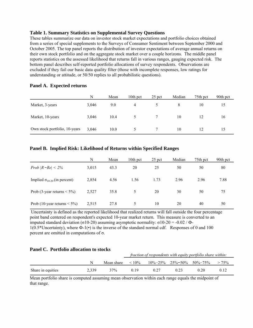
Table 1. Summary Statistics on Supplemental Survey Questions These tables summarize our data on investor stock market expectations and portfolio choices obtained from a series of special supplements to the Surveys of Consumer Sentiment between September 2000 and October 2005. The top panel reports the distribution of investor expectations of average annual returns on their own stock portfolio and on the aggregate stock market over a couple horizons. The middle panel reports statistics on the assessed likelihood that returns fall in various ranges, gauging expected risk. The bottom panel describes self-reported portfolio allocations of survey respondents. Observations are excluded if they fail our basic data quality filter (those with incomplete responses, low ratings for understanding or attitude, or 50/50 replies to all probabilistic questions). Panel A. Expected returns

N Mean 10th pct 25 pct Median 75th pct 90th pct

Market, 3-years 3,046 9.0 4 5 8 10 15

Market, 10-years 3,046 10.4 5 7 10 12 16

Own stock portfolio, 10-years 3,046 10.0 5 7 10 12 15

Panel B. Implied Risk: Likelihood of Returns within Specified Ranges

N Mean 10th pct 25 pct Median 75th pct 90th pct

Prob |R−Re| < 2% 3,015 43.3 20 25 50 50 80

Implied σ10-20 (in percent) 2,854 4.56 1.56 1.73 2.96 2.96 7.88

Prob (3-year returns < 5%) 2,527 35.8 5 20 30 50 75

Prob (10-year returns < 5%) 2,515 27.8 5 10 20 40 50

Uncertainty is defined as the reported likelihood that realized returns will fall outside the four percentage point band centered on respondent's expected 10-year market return. This measure is converted to an imputed standard deviation (σ10-20) assuming asymptotic normality: σ10-20 = -0.02 / Ф-1(0.5*Uncertainty), where Ф-1(•) is the inverse of the standard normal cdf. Responses of 0 and 100 percent are omitted in computations of σ. Panel C. Portfolio allocation to stocks

N Mean share < 10% 10%−25% 25%−50% 50%−75% > 75%

Share in equities 2,339 37% 0.19 0.27 0.23 0.20 0.12

fraction of respondents with equity portfolio share within:

Mean portfolio share is computed assuming mean observation within each range equals the midpoint of that range.

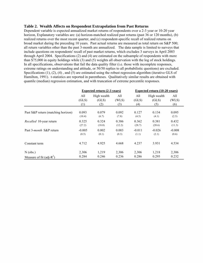
Table 2. Wealth Affects on Respondent Extrapolation from Past Returns Dependent variable is expected annualized market returns of respondents over a 2-3 year or 10-20 year horizon, Explanatory variables are: (a) horizon-matched realized past returns (past 36 or 120 months), (b) realized returns over the most recent quarter, and (c) respondent-specific recall of realized returns on broad market during the preceding 10 years. Past actual returns are measured as total return on S&P 500; all return variables other than the past 3-month are annualized. The data sample is limited to surveys that include questions on respondents' recall of past market returns, which excludes 3 surveys in April 2003 through April 2004. Specifications (2) and (4) are estimated on the subsample of respondents with more than $75,000 in equity holdings while (3) and (5) weights all observation with the log of stock holdings. In all specifications, observations that fail the data quality filter (i.e. those with incomplete responses, extreme ratings on understanding and attitude, or 50/50 replies to all probabilistic questions) are excluded. Specifications (1), (2), (4) , and (5) are estimated using the robust regression algorithm (iterative GLS of Hamilton, 1991). t-statistics are reported in parentheses. Qualitatively similar results are obtained with quantile (median) regression estimation, and with truncation of extreme percentile responses.

All (GLS)

High wealth (GLS)

All (WLS)

All (GLS)

High wealth (GLS)

All (WLS)

(1) (2) (3) (4) (5) (6)

Past S&P return (matching horizon) 0.093 0.079 0.092 0.127 0.134 0.095(10.4) (6.7) (7.8) (4.5) (4.1) (2.5)

Recalled 10-year return 0.325 0.324 0.386 0.362 0.381 0.432(27.2) (18.0) (12.2) (28.7) (20.6) (11.3)

Past 3-month S&P return -0.005 0.002 0.003 -0.011 -0.026 -0.008(0.5) (0.1) (0.3) (1.1) (2.1) (0.6)

Constant term 4.712 4.925 4.668 4.237 3.931 4.534

N (obs.) 2,306 1,219 2,306 2,306 1,218 2,306Measure of fit (adj-R2) 0.284 0.246 0.236 0.286 0.295 0.232

Expected return (10-20 years)Expected return (2-3 years)

Table 3. Heterogeneity in macroeconomic and own income growth expectations This table summarizes the distribution of investor responses to certain Michigan Survey questions on macroeconomic outlook. The top panel tabulates investor responses to questions on expected economic conditions over next 5 years. The surveys are chosen to coincide with some of the key events over the sample period: the peak of the bull market (September 2000), the 9/11 attacks (October 2001), the start of the Iraq war (April 2003), and hurricane Katrina (October 2005). The lower panel reports (for selected surveys) Spearman rank correlations among this variable and two other gauges of respondent outlook: expected change in business conditions over next 12 months, and percent chance own income outpaces inflation over next 5 years. The bottom two lines show correlations of these outlook measures with expected stock market returns. The first figure in each pair is calculated on microdata pooled across surveys; the second figure (after semicolon) is calculated using survey-specific means, and thus gauges time-series correlation. Panel A. Distribution of responses, select surveys

September, 2000 October, 2001 April, 2003 October, 2005

Continuous bad times 0.09 0.28 0.21 0.52

Bad times, qualified 0.04 0.14 0.12 0.08

Uncertain / Pro-con 0.04 0.07 0.05 0.06

Good times, qualified 0.10 0.09 0.10 0.02

Continuous good times 0.74 0.43 0.51 0.32

Expected macroeconomic conditions over the next 5 years (fraction of respondents answering …)

Panel B. Correlation between measures of expected conditions and expected returns, pooled data; times-series means

Good times, next 5 years

Better conditions, next 12 mo.

Chance own income outpaces inflation

Good times, next 5 years

Better conditions, next 12 mo. 0.42**

Chance own income outpaces inflation 0.26** 0.23**

Expected returns (2-3 years) 0.18** ; 0.66** 0.12** ; -0.39 0.11** ; 0.41

Expected returns (10-20 years) 0.11** ; 0.67** 0.11** ; -0.13 0.10** ; 0.44** ** indicates statistical significance at the 5 percent level.

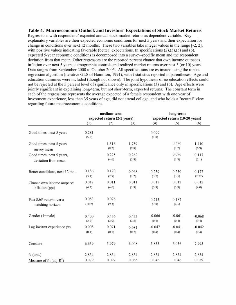
Table 4. Macroeconomic Outlook and Investors' Expectations of Stock Market Returns Regressions with respondents' expected annual stock market returns as dependent variable. Key explanatory variables are their expected economic conditions for next 5 years and their expectation for change in conditions over next 12 months. These two variables take integer values in the range [-2, 2], with positive values indicating favorable (better) expectations. In specifications (2),(3),(5) and (6), expected 5-year economic conditions is decomposed into a survey-specific mean and the respondent deviation from that mean. Other regressors are the reported percent chance that own income outpaces inflation over next 5 years, demographic controls and realized market returns over past 3 (or 10) years. Data ranges from September 2000 to October 2005. All specifications are estimated using the robust regression algorithm (iterative GLS of Hamilton, 1991), with t-statistics reported in parentheses. Age and education dummies were included (though not shown). The joint hypothesis of no education effects could not be rejected at the 5 percent level of significance only in specifications (3) and (6). Age effects were jointly significant in explaining long-term, but not short-term, expected returns. The constant term in each of the regressions represents the average expected of a female respondent with one year of investment experience, less than 35 years of age, did not attend college, and who holds a "neutral" view regarding future macroeconomic conditions.

(1) (2) (3) (4) (5) (6)

Good times, next 5 years 0.281 0.099(5.8) (1.8)

Good times, next 5 years 1.516 1.759 0.376 1.410 survey mean (8.2) (9.8) (1.2) (6.9)

Good times, next 5 years, 0.225 0.262 0.096 0.117 deviation from mean (4.6) (5.8) (1.8) (2.1)

Better conditions, next 12 mo. 0.186 0.170 0.068 0.239 0.230 0.177(3.1) (2.9) (1.2) (3.7) (3.5) (2.72)

Chance own income outpaces 0.012 0.011 0.011 0.012 0.012 0.012 inflation (ppt) (4.3) (4.0) (3.9) (3.9) (3.9) (4.0)

Past S&P return over a 0.083 0.076 0.215 0.187 matching horizon (10.2) (9.3) (7.8) (4.5)

Gender (1=male) 0.400 0.436 0.433 -0.066 -0.061 -0.068(2.7) (2.9) (2.8) (0.4) (0.4) (0.4)

Log invstmt experience yrs 0.008 0.071 0.081 -0.047 -0.041 -0.042(0.1) (0.7) (0.7) (0.4) (0.4) (0.4)

Constant 6.639 5.979 6.048 5.833 6.056 7.995

N (obs.) 2,834 2,834 2,834 2,834 2,834 2,834Measure of fit (adj-R2) 0.079 0.097 0.065 0.046 0.046 0.039

medium-term long-termexpected return (2-3 years) expected return (10-20 years)

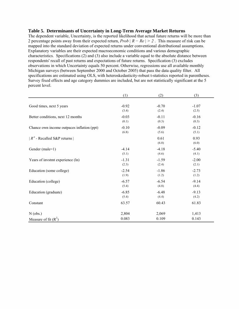
Table 5. Determinants of Uncertainty in Long-Term Average Market Returns The dependent variable, Uncertainty, is the reported likelihood that actual future returns will be more than 2 percentage points away from their expected return, Prob | R − Re | > 2 . This measure of risk can be mapped into the standard deviation of expected returns under conventional distributional assumptions. Explanatory variables are their expected macroeconomic conditions and various demographic characteristics. Specifications (2) and (3) also include a variable equal to the absolute distance between respondents' recall of past returns and expectations of future returns. Specification (3) excludes observations in which Uncertainty equals 50 percent. Otherwise, regressions use all available monthly Michigan surveys (between September 2000 and October 2005) that pass the data quality filter. All specifications are estimated using OLS, with heteroskedasticity-robust t-statistics reported in parentheses. Survey fixed effects and age category dummies are included, but are not statistically significant at the 5 percent level. (1) (2) (3)

Good times, next 5 years -0.92 -0.70 -1.07(3.4) (2.4) (2.5)

Better conditions, next 12 months -0.03 -0.11 -0.16(0.1) (0.3) (0.3)

Chance own income outpaces inflation (ppt) -0.10 -0.09 -0.12(6.8) (5.6) (5.1)

| R e - Recalled S&P returns | 0.61 0.93(6.0) (6.0)

Gender (male=1) -4.14 -4.18 -5.40(5.1) (4.6) (4.1)

Years of invstmt experience (ln) -1.31 -1.59 -2.00(2.3) (2.4) (2.1)

Education (some college) -2.54 -1.86 -2.73(1.9) (1.2) (1.2)

Education (college) -6.57 -6.54 -9.14(5.4) (4.8) (4.4)

Education (graduate) -6.85 -6.48 -9.13(5.4) (4.4) (4.2)

Constant 63.57 60.43 61.83

N (obs.) 2,804 2,069 1,413Measure of fit (R2) 0.083 0.109 0.143

Table 6. Investor Expectations and Portfolio Choice Top panel shows Sharpe ratios: expected own portfolio return over annual standard deviation of market returns (imputed from Uncertainty). Means and medians are shown for observations grouped by portfolio equity exposures. p-values are for tests of differences in median group Sharpe ratio relative to the middle group (25 to 50 percent exposure). The bottom panel reports regressions of respondents' portfolio equity share on expected own stock portfolio return and imputed variance of stock market returns. Data from Michigan surveys with question on portfolio composition (June 2001 and later). All regressions exclude observations with extreme values of expected return (2nd and 98th percentile cutoffs) or volatility (Uncertainty equal to 0 or 100 percent). Regression (1) excludes households with negative expected excess return. Estimates are OLS, with heteroskedasticity-robust t-statistics reported in parentheses. Time dummies (not reported) are jointly significant; age dummies are jointly significant in all but (4). Panel A. Forward-looking Sharpe ratios by portfolio exposure to equity

p -valueShare invested in equities N Mean Median (H0: SR≠SR25-50)

Less than 10 percent 415 0.475 0.309 (0.000)

Between 10 and 25 percent 591 0.550 0.401 (0.007)

Between 25 and 50 percent 490 0.631 0.505

Between 50 and 75 percent 430 0.654 0.525 (0.646)

More than 75 percent 256 0.701 0.623 (0.015)

forward-looking Sharpe Ratios

Panel B. Regression of portfolio equity exposure on expected risk and return

Regressors (1) (2) (3) (4)

Log expected excess returns 0.04(1.9)

Log expected returns 0.15(3.4)

Expected excess returns (in pct) 0.33 0.28(2.6) (2.2)

Log expected volatility (σi2) -0.09 -0.09

(6.6) (7.1)

Uncertainty (in pct) -0.22 -0.20(8.1) (7.4)

Years of invstmt experience (ln) 0.07(7.7)

Constant -1.90 -1.84 0.41 0.27

N (obs.) 1,995 2,182 2,182 2,176Measure of fit (adj-R2) 0.042 0.046 0.047 0.074

portfolio fraction in stockslog portfolio fraction in stocks