Unemployment Expectations, Jumping (S,s) Triggers, … · Unemployment Expectations, Jumping (S,s)...

Comments Welcome

Unemployment Expectations, Jumping (S,s) Triggers,

and Household Balance Sheets

Forthcoming, NBER Macroeconomics Annual, 1997

Christopher D. Carroll†

[email protected]

Wendy E. Dunn‡

[email protected]

May 30, 1997

Keywords: uncertainty, housing, motor vehicles, consumption, (S,s) models, unemployment, expec-tations, balance sheets

JEL Codes: D1, D8, D9, E2, E3

AbstractThis paper examines the relationship between household balance sheets, consumer purchases, andexpectations. We find few robust empirical relationships between balance sheet measures and spend-ing, but we do find that unemployment expectations are robustly correlated with spending. We thenconstruct a formal model of durables and nondurables consumption with an explicit role for unem-ployment and for household debt. We find that the model is capable of explaining several empiricalregularities which are, at best, unexplained by standard models. Finally, we show that a looseningof liquidity constraints can produce a runup in debt similar to that experienced recently in the US,and that after such a liberalization consumer purchases show heightened sensitivity to labor incomeuncertainty, providing a potential rigorous interpretation of the widespread view that the buildup ofdebt in the 1980s may have played an important role in the weakness of consumption during and afterthe 1990 recession.

We are grateful to Carl Christ, Darrel Cohen, Russell Cooper, Angus Deaton, Karen Dynan, Janice Eberly,Bruce Fallick, James Fergus, Jonas Fisher, Michael Fratantoni, Simon Gilchrist, John Leahy, Jonathan Mc-Carthy, Spencer Krane, Sydney Ludvigson, Greg Mankiw, Randy Mariger, Louis Maccini, David Reifschnei-der, Martha Starr-McCluer, Daniel Sichel, and seminar participants at Johns Hopkins University, the Boardof Governors of the Federal Reserve System, and the 1997 NBER Macroeconomics Annual conference forvaluable comments and all sorts of help.

The set of RATS programs that generate all of our empirical results, the set of Mathematica programsthat generate all of our theoretical results, and a companion paper describing details of our empirical andtheoretical methodolgy are all available at Carroll’s home page, http://www.econ.jhu.edu/ccarroll.

† NBER and The Johns Hopkins University. Correspondence to Christopher Carroll, Department ofEconomics, Johns Hopkins University, Baltimore, MD 21218-2685 or [email protected].

‡ Department of Economics, Johns Hopkins University.

Abstract

This paper examines the relationship between household balance sheets, consumer purchases,

and expectations. We find few robust empirical relationships between balance sheet measures and

spending, but we do find that unemployment expectations are robustly correlated with spending.

We then construct a formal model of durables and nondurables consumption with an explicit role

for unemployment and for household debt. We find that the model is capable of explaining several

empirical regularities which are, at best, unexplained by standard models. Finally, we show that a

loosening of liquidity constraints can produce a runup in debt similar to that experienced recently

in the US, and that after such a liberalization consumer purchases show heightened sensitivity to

labor income uncertainty, providing a potential rigorous interpretation of the widespread view that

the buildup of debt in the 1980s may have played an important role in the weakness of consumption

during and after the 1990 recession.

1

1 Introduction

The US recession that began in 1990 and the feeble recovery that followed differed from the pat-

tern of previous postwar business cycles in several respects, most notably in the sustained weakness in

consumption spending, particularly for durable goods. Blanchard (1993) estimates a simple macroeco-

nomic model and finds that the recession was largely the result of a “consumption shock.” Hall (1993)

finds an important role for a ‘spontaneous decline in consumption,’ especially for durable goods.

Furthermore, structural macroeconomic models like the FRB-US model substantially overpredicted

consumption spending throughout the 1990 recession and especially the early recovery period.

In December 1991, as the economy struggled to make its way out of recession, Federal Reserve

Chairman Alan Greenspan included the following statements in Congressional testimony on the state

of the economy:

During the 1980s, large stocks of physical assets were amassed in a large number of sectors,

largely financed by huge increases in indebtedness.... In the household sector, purchases of

motor vehicles and other consumer durables ran for several years at remarkably high levels

and were often paid for with installment or other debt that carried extended maturities.

In some parts of the United States, the household spending boom reached to the purchase

of homes. . . . The aftermath of all this activity is a considerable degree of financial stress

in the household sector. (Greenspan (1992)).

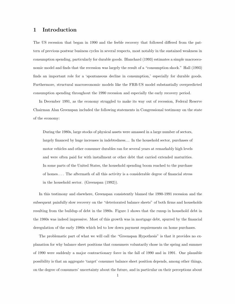
In this testimony and elsewhere, Greenspan consistently blamed the 1990-1991 recession and the

subsequent painfully slow recovery on the “deteriorated balance sheets” of both firms and households

resulting from the buildup of debt in the 1980s. Figure 1 shows that the runup in household debt in

the 1980s was indeed impressive. Most of this growth was in mortgage debt, spurred by the financial

deregulation of the early 1980s which led to low down payment requirements on home purchases.

The problematic part of what we will call the “Greenspan Hypothesis” is that it provides no ex-

planation for why balance sheet positions that consumers voluntarily chose in the spring and summer

of 1990 were suddenly a major contractionary force in the fall of 1990 and in 1991. One plausible

possibility is that an aggregate ‘target’ consumer balance sheet position depends, among other things,

on the degree of consumers’ uncertainty about the future, and in particular on their perceptions about1

1962 1967 1972 1977 1982 1987 1992

0.6

0.7

0.8

0.9

1.0

1.1

1.2

Figure 1: Debt To Income Ratio

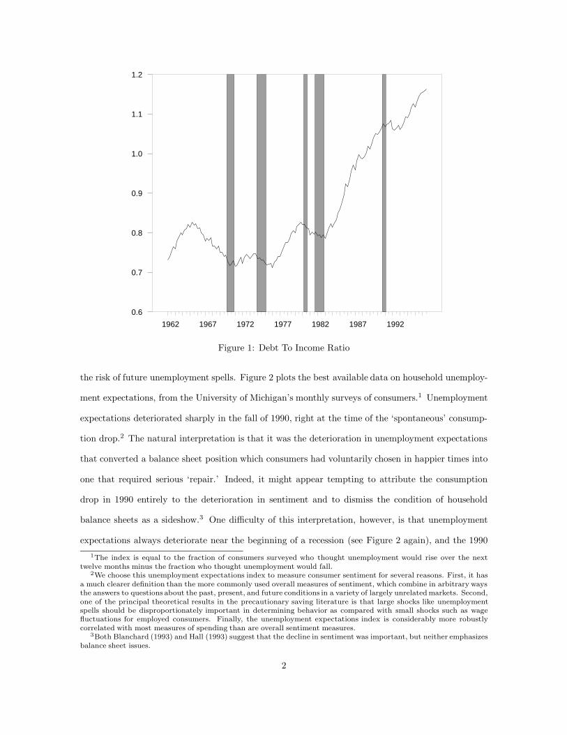
the risk of future unemployment spells. Figure 2 plots the best available data on household unemploy-

ment expectations, from the University of Michigan’s monthly surveys of consumers.1 Unemployment

expectations deteriorated sharply in the fall of 1990, right at the time of the ‘spontaneous’ consump-

tion drop.2 The natural interpretation is that it was the deterioration in unemployment expectations

that converted a balance sheet position which consumers had voluntarily chosen in happier times into

one that required serious ‘repair.’ Indeed, it might appear tempting to attribute the consumption

drop in 1990 entirely to the deterioration in sentiment and to dismiss the condition of household

balance sheets as a sideshow.3 One difficulty of this interpretation, however, is that unemployment

expectations always deteriorate near the beginning of a recession (see Figure 2 again), and the 19901The index is equal to the fraction of consumers surveyed who thought unemployment would rise over the next

twelve months minus the fraction who thought unemployment would fall.2We choose this unemployment expectations index to measure consumer sentiment for several reasons. First, it has

a much clearer definition than the more commonly used overall measures of sentiment, which combine in arbitrary waysthe answers to questions about the past, present, and future conditions in a variety of largely unrelated markets. Second,one of the principal theoretical results in the precautionary saving literature is that large shocks like unemploymentspells should be disproportionately important in determining behavior as compared with small shocks such as wagefluctuations for employed consumers. Finally, the unemployment expectations index is considerably more robustlycorrelated with most measures of spending than are overall sentiment measures.

3Both Blanchard (1993) and Hall (1993) suggest that the decline in sentiment was important, but neither emphasizesbalance sheet issues.

2

1961 1966 1971 1976 1981 1986 1991

-0.48

-0.32

-0.16

0.00

0.16

0.32

0.48

0.64

Figure 2: Unemployment Expectations

experience was not sufficiently different from previous recessions to explain why consumption growth

was weaker than it usually is during recessions. The behavior of the unemployment expectations index

was more unusual after the trough of the recession; usually the index plummets just after the trough,

but unemployment expectations remained quite high for a long time after the 1991 trough.4 Still,

even consumption models which incorporate the unemployment expectations index have large nega-

tive residuals during and after the 1990 recession, implying that the consumption weakness cannot be

explained as simply reflecting consumer pessimism.

Prompted by this debate, this paper is a broad attempt to make sense of the relationship between

household balance sheets, unemployment expectations, and household purchases. We begin (in Sec-

tion 2) by documenting what we take to be the main stylized facts about the empirical relationships

between consumer purchases, household balance sheets, and uncertainty. The only systematic rela-

tionship we are able to uncover between balance sheet measures and spending is a robust positive

correlation between lagged debt growth and the current level of spending on durables, a relationship4It is interesting to note that the index was ‘right’, in the sense that the unemployment rate did remain unusually

high for an unusually long period after the trough.

3

which is most easily interpreted as reflecting simultaneity rather than a causal link. However, we do

identify another empirical regularity: our preferred measure of uncertainty, the lagged value of the

Unemployment Expectations index plotted in Figure 2, is robustly correlated with every measure of

consumer spending, even after controlling for ‘permanent income’ as best we can (and in particular

after controlling for whatever information unemployment expectations contain about future income).

With these results in mind, we then (in Section 3) construct a theoretical model of the durable

goods purchase problem for consumers who face the possibility of unemployment spells. Because

analytical solutions are not available when there is labor income uncertainty, we solve the model

numerically. We find that the model implies that a rise in uncertainty causes consumers to delay

durables purchases (formally, the lower trigger of the (S,s) rule jumps down; hence our title). We then

compare simulation results from the model with our empirical evidence for the US economy, and find

that the model explains some but not all of the empirical findings. In particular, the model implies

a much stronger role for changes in unemployment expectations, and a weaker role for the lagged

level of unemployment expectations, than we find in the data. Finally, in Section 6, we show that

the model implies that a financial liberalization which loosens liquidity constraints will cause a runup

in aggregate debt like the runup shown in figure 1, and that in the liberalized economy the reaction

of durables purchases to uncertainty is intensified. Thus our model potentially rationalizes the idea

that the runup of consumer debt in the 1980s was partly responsible for the puzzling weakness of

consumption spending during and after the 1990 recession. Furthermore, the model implies that the

continuing growth of the debt ratio may be making consumption increasingly vulnerable to swings in

consumer sentiment.

2 Empirical Results

2.1 Balance Sheets and Nondurables Consumption Growth

Although housing and other durable goods account for most of the volatility of consumption spending

over the business cycle, we begin our empirical work by examining spending on nondurable goods.

Partly this is because virtually no existing work has examined the effect of either balance sheets or

time-varying unemployment expectations on nondurables spending, and these are important questions

in their own right. Partly, we examine nondurables because one of the innovations of our theoretical

4

model is our joint treatment of durables and nondurable goods.5 Thus, in principle, even in the absence

of time-varying unemployment risk our model might generate different predictions for nondurables

spending than standard models.

The benchmark model with which we intend to compare both empirical results and the theoretical

predictions of our model is the representative agent, certainty equivalent version of the Permanent

Income model (henceforth, CEQ PIH model), as used, for example, by Campbell (1987), Campbell

and Deaton (1989), and many others. In this model, consumption is equal to “permanent income”

defined as the annuity value of total wealth, human and nonhuman:

Ct =r

1 + r[W h

t + Wnt ]

W ht =

∞∑s=t

(1

1 + r

)s−tYs

where Ys is total noncapital income (labor income plus net transfers) in period s. We define a variable

which we will call “annuity labor income” At as the annuity value of human wealth:6

At =r

1 + rW ht .

As Hall (1978) famously pointed out, one of the implications of this model is that lagged informa-

tion should have no predictive power for current consumption growth. Campbell and Mankiw (1989)

showed that all of the empirical failures of the CEQ PIH model could be explained by a model in

which a fraction λ of aggregate labor income goes to rule-of-thumb consumers who simply spend all

available income in each quarter while (1−λ) of income accrues to consumers who behave according to

the CEQ PIH model. These assumptions, plus a few approximations, lead to an estimating equation

of the form:

∆ logCt = γ0 + γ1Et−1∆ logYt + εt,

where the expectation is taken with respect to a set of instruments dated t − 1.7 Because, strictly5Most previous modelling efforts, with the exception of Bernanke (1985), have assumed utility flows either solely

from nondurables or solely from durables, or at the very least that utility from durables and nondurables is separable.6We adopt this terminology partly to avoid confusion between the variable in this model and the “permanent labor

income” variable in our theoretical model.7Because time aggregation can introduce an MA(1) error term, the usual procedure is to use instruments dated t−2.

However, as Carroll, Fuhrer, and Wilcox (1994) argue, this unnecessarily discards potentially valuable information invariables dated t − 1. We follow those authors in pursuing a nonlinear estimation methodology that allows us to useinstruments dated t − 1 and to impose the orthogonality restriction directly. Our instruments for income growth arethe same as those used by Carroll, Fuhrer, and Wilcox (1994): three lags each of income growth, consumption growth,

5

speaking, the model applies only to the consumption of nondurables, our measure of consumption is

spending on nondurable goods from the NIPA accounts.8

Results are contained in Table 1. Our first regression reproduces the basic result of Campbell

and Mankiw (1989): the coefficient on predictable income growth is enormously statistically signif-

icant (with a t-statistic of over 4), and suggests that rule-of-thumb consumers earn roughly half of

aggregate labor income. Our second regression performs a simple Hall-style test of whether lagged

unemployment expectations are useful in predicting current consumption growth. Again the answer

is overwhelmingly yes; the t-statistic is 3.7. Our next regression reconfirms the main result of Carroll,

Fuhrer, and Wilcox (1994): the lagged level of consumer sentiment (as measured by unemployment

expectations) contains substantial predictive power for consumption growth even after controlling for

the information sentiment contains about income growth.910

Turning now to the role of balance sheet variables, our goal is to test whether such variables

violate the benchmark sentiment-augmented Campbell-Mankiw model presented in row 3 of Table 1.

In our background empirical work we examined a broad set of measures of household balance sheet

conditions, but in the paper we present results for only three measures: the ratio of liabilities to

annuity labor income, the ratio of liabilities to assets, and the growth rate of liabilities.11 None of

the other balance sheet variables we examined performed better (in the sense of being more highly

correlated with the dependent variables we are interested in) than these three variables.12

the change in the three-month T-bill rate, the change in the unemployment rate, and the growth of the S&P 500 index,one lag of the log difference between consumption and income and of the measure of sentiment being tested (in ourcase, unemployment expectations; in the Carroll, Fuhrer, Wilcox paper, overall consumer sentiment). The adjusted R2

on the first-stage regression for income growth is 0.41.8The model is often estimated on the sum of nondurables and services consumption. However, in the ‘final’ version

of NIPA data, substantial parts of services consumption are constructed using quarterly interpolation through annualestimates, where the later endpoint for the interpolation is strictly in the future of some of the quarterly estimates ofservices spending it is used to construct. This potentially introduces spurious time-series properties into the servicescomponent of spending which are most easily avoided by excluding services from the measure of consumption. For morediscussion of these points, see Wilcox (1992).

9Carroll, Fuhrer, and Wilcox used the overall index of consumer sentiment rather than the unemployment expecta-tions index we use here; also, they tested for the joint significance of four lags of sentiment, rather than just a single lagas we do.

10When lagged unemployment expectations are added to the Campbell-Mankiw equation, the coefficient estimateon forecastable income growth is about half of its previous value and just misses being statistically significant (thep-value is .103). The reason the statistical significance of the forecastable part of income growth drops so dramaticallywhen lagged unemployment expectations are included in the regression is that lagged unemployment expectations arehighly correlated with the forecastable component of income growth. Whether income growth is significant, laggedunemployment expectations are signficant, or neither is significant is somewhat sensitive to the choice of instruments;in particular, if the instrument set does not contain variables that provide substantial information about income growththat is independent of the information about income growth contained in unemployment expectations, typically neitherincome growth nor unemployment expectations is individually significant.

11See below for a discussion of how we constructed our estimate of annuity labor income.12We also examined the ratio of debt to net worth, the ratio of debt to liquid assets, the ratio of debt to current

income, and the ratio of the debt service burden to annuity income, among others.

6

Nondurable Consumption GrowthQuarterly Data, 1963:3-1994:3

BalanceSheet Balance

Row Measure Et−1∆ logYt UEt−1 Sheet θ SSR D-W1 0.509 0.086 0.49 1.98

(4.13)∗∗∗ (0.93)2 −1.310 0.136 0.58 1.97

−(3.69)∗∗∗ (1.47)3 0.269 −0.906 0.092 0.50 1.98

(1.64) −(2.18)∗∗ (0.99)4 ∆ logDt−1 0.246 −0.690 0.095 0.088 0.49 2.00

(1.50) −(1.55) (1.33) (0.94)5 rDt−1/Yt−1 0.257 −0.820 −0.073 0.0937 0.49 1.98

(1.57) −(1.90)∗ −(0.93) (1.00)6 Dt−1/At−1 0.247 −0.906 −0.002 0.096 0.50 1.97

(1.45) −(2.15)∗∗ −(0.33) (1.02)∗ Significant at 10% or better. ∗∗ Significant at 5% or better. ∗∗∗ Significant at 1% or better.

Notes: t statistics are listed in parentheses below coefficient estimates. Yt is total household wage and transfer income.UEt−1 is the unemployment expectations index. The instruments are the same as the second set used in Carroll, Fuhrer, andWilcox (1994). The balance sheet variables are the growth in total household liabilities (∆ logDt−1), the debt service burden(rDt−1/Yt−1), and the ratio of total household liabilities to annuity income (Dt−1/At−1). θ is the estimated coefficient onthe moving average error term. A constant term was also included but is not reported.

Table 1: The Sentiment-Augmented Campbell-Mankiw Model

Our empirical test is simply whether lagged balance sheet variables are statistically significant when

we add them to the sentiment-augmented Campbell-Mankiw model.13 As rows 4 through 6 of the table

show, none of the balance sheet variables is statistically significant in any of the regressions.14 Thus,

there is little evidence that household balance sheet conditions have any influence on nondurables

consumption growth that operates through any channel outside of the sentiment-augmented Campbell-

Mankiw model.15

We now turn to the question of the relative importance for nondurables consumption of innovations

to annuity income and to unemployment expectations. This question is of central importance to the13Of course, we also add them to the set of instruments used for predicting income growth.14The debt to annuity income variable appears to be nonstationary, while consumption growth is approximately

stationary; econometric theory implies that for a large enough time sample, the coefficient in a regression of a stationaryvariable on a nonstationary one must yield a zero coefficient, so the insignificance of this variable is hardly surprising.

15These results are somewhat at variance with previous results of Ludvigson (1996), who found that predictable debtgrowth was significantly related to consumption growth. We were able to reproduce Ludvigson’s results, and havedetermined that there are four reasons for the differences in outcomes. First, our measure of consumption spendingis restricted to nondurable goods, while Ludvigson followed most of the previous literature by examining spending onnondurable goods and services. We believe that the data construction methods for the quarterly services expendituresrender those data unsuitable for regressions of this kind. Second, because our focus is on the overall structure ofhousehold balance sheets, our measure of debt is total household liabilities, while Ludvigson’s balance sheet variable wasconsumer installment credit, i.e. mainly debt exclusive of mortgages. Third, Ludvigson’s test was whether consumptiongrowth was related to predictable debt growth, while our test is a more direct test of the Campbell-Mankiw model:whether lagged debt growth matters. Finally, Ludvigson was using the standard Campbell-Mankiw model as her baselinerather than the sentiment-augmented model we are using (although our result that lagged debt growth is insignificantholds up even when we estimate a standard (non-sentiment-augmented) Campbell-Mankiw model).

7

enterprise of this paper because the answer should help to inform us whether ignoring fluctuations

in uncertainty is a small omission that is well worth the associated modelling dividend of analytical

tractability, or a large omission, so that any model which ignores uncertainty is likely to tell a seriously

incomplete story about the determinants of consumption over the business cycle.

To examine this issue (and many others we will introduce later in the paper) we need an estimate

of the level of annuity income. We construct two estimates, first following a method used to estimate

annuity personal disposable income in the FRB-US model at the Federal Reserve Board, then using a

method of our own devising. The FRB-US methodology (AFRB-USt ) is based on an assumption that the

ratio of personal income to GDP is stationary and that the GDP gap is stationary. A VAR forecasting

system is used to estimate the projected future output gap XGAP and the projected future gap in the

ratio of income to GDP, YGAP. The VAR system includes equations for inflation, the fed funds rate,

XGAP, and YGAP. We also added four lags of income growth and the unemployment expectations

variable to each equation.16

Our own annuity labor income measure (AOurst ) is created by forecasting the present discounted

value of the sum of the next two years of labor income using a set of forecasting variables drawn

from the Carroll, Fuhrer, and Wilcox (1994) set of instruments for income growth. We make the

assumption that beyond two years income is expected to grow at a constant rate equal to the average

growth rate over the entire sample period. Using this growth rate, we calculate the annuity value of

income from two years to infinity and add this to the forecasted discounted sum of income over the

next two years to get AOurst . For more details on the two methods of constructing annuity income, see

the companion methodology paper Carroll and Dunn (1997).

In principle, if our estimate of the innovation to annuity income were perfect (or, more realistically,

if the variables we use to construct the measure are valid instruments for annuity income growth) then

the following equation would characterize nondurable consumption growth in the Campbell-Mankiw

model:

∆ logCt = (1− λ)Et−1ρ−1(rt − δ) + λ∆ logYt + (1− λ)∆ logAt (1)

Hence we could obtain an estimate of the fraction of income accruing to CEQ PIH income consumers16We are grateful to David Reifschneider at the Federal Reserve for explaining the FRB-US methodology to us.

Because we are adapting the FRB-US methodology to a purpose quite different from its intended purpose, and becausewe are using a different measure of income, any empirical inadequacies of the annuity income measure we constructusing the FRB-US methodology should be laid at our doorstep, not the FRB-US model staff’s.

8

Nondurable Consumption GrowthQuarterly Data, 1963:3-1994:3

Row ∆ logYt ∆ logAOurst ∆ logAFRB-US

t UEt−1 ∆UEt R2

D-W1 0.326 0.186 −0.833 0.33 1.83

(3.15)∗∗∗ (2.82)∗∗∗ −(2.55)∗∗∗

2 0.324 0.124 −1.003 −0.907 0.34 1.92(3.15)∗∗∗ (1.59) −(2.92)∗∗∗ −(1.52)

3 0.391 0.189 −0.654 0.29 1.92(3.41)∗∗∗ (1.20) −(2.00)∗∗

4 0.394 0.000 −0.981 −1.413 0.32 2.00(3.50)∗∗∗ (0.00) −(2.83)∗∗∗ −(2.47)∗∗

∗ Significant at 10% or better. ∗∗ Significant at 5% or better. ∗∗∗ Significant at 1% or better.

Notes: t statistics are listed in parentheses below coefficient estimates. Standard errors were constructed using a serialcorrelation-robust covariance matrix (allowing serial correlation at lags up to 8). Yt is total household wage and transferincome. At is annuity labor income. UEt−1 is the unemployment expectations index. A constant term was also includedbut is not reported.

Table 2: Effects of Innovations on Nondurables Consumption

from the coefficient on actual current income growth in a regression of consumption growth on current

income growth and the current innovations to annuity income.17 Table 2 presents the results when

equation (1) is estimated using our two measures of annuity income.

The first regression shows that the lagged level of UE and the current innovation to our measure of

annuity income are roughly equally important in explaining current consumption growth. The second

regression shows that when the current innovation to UE is added to the equation, neither it nor the

innovation to annuity income is individually statistically significant; however, the lagged level of UE

remains important. The last two regressions show that, after controlling for unemployment expec-

tations, the FRB-US measure of annuity income provides no further information about consumption

growth at all.

In sum, the standard model of nondurable consumption growth, the Campbell-Mankiw model, im-

plies that consumption growth should be related to two variables: income growth and the innovations

to annuity income. Our empirical work shows that unemployment expectations are at least as impor-

tant as either of these traditional variables in explaining nondurables consumption growth. Lagged

balance sheet variables, on the other hand, are essentially uncorrelated with nondurable consumption

growth once unemployment expectations are controlled for.17This point relies heavily on the assumption that our estimate of annuity income growth correctly captures all the

implications for annuity income of the innovation to current income. However, we do include current income growthamong the variables used to construct annuity income, so in principle any such information is indeed included.

9

2.2 Balance Sheets and Spending on Durable Goods and Housing

The standard CEQ PIH model described above applies to consumption of nondurable goods and

services. However, as Mankiw (1982) showed, the model can be expanded to provide implications

about durable goods spending if sufficient assumptions are made. In particular, if there are no

transactions costs associated with durable goods purchases and if durable goods enter the utility

function in a Cobb-Douglas manner, it is possible to show that the ratio of the stock of durable goods

Zt to annuity income At should be constant:18

Zt = ωAt. (2)

Expenditure on durable goods in this case will be determined by two factors: the spending needed

to counteract depreciation, and the spending required to adjust the stock of durable goods to any

changes in the level of annuity income:

Ezt = Zt − (1− δ)Zt−1 (3)

Ezt /At = ω − (1− δ)ωAt−1/At. (4)

Table 3 presents empirical results when we estimate an equation like (4) using US NIPA data on

durables expenditures, augmented with UEt−1 and ∆UEt. We also include: the ratio of current

income to annuity income to allow some scope for current income to affect spending directly; the

prime rate to allow a channel for interest rates; and the ratio of net worth to annuity income (not

shown in the table to save space; it was usually not statistically significant). We present results

separately for our estimate of annuity income, the annuity income estimate based on the FRB-US

methodology, and the analogous results where we use current income rather than an estimate of

annuity income.19 We experimented with several methods of removing low-frequency movements or

trends in the data, but they had little effect and are therefore not included.20

18The assumption of frictionless adjustment is of course unattractive for durable goods, as many authors have pointedout. For an excellent discussion of the literature and of the difficulties, see Bertola and Caballero (1990), who also proposea sophisiticated (and complicated) method of estimating the process for durables expenditures under a generalized (S,s)model with fixed return points. See also Bertola and Caballero (1994) and Eberly (1997). For reasons that will becomeclear in the theoretical discussion below, however, these frameworks are not well suited to addressing the issues weare interested in here of the relationship between labor income uncertainty, balance sheet variables, and spending.We therefore adopt the approach of estimating as simple an empirical model as possible, with an eye to finding anycorrelations sufficiently robust that any theoretical model should be consistent with them.

19For the Yt/At variable, we use the ratio of current income to our estimate of annuity income.20The Durbin-Watson statistics in the table indicate a large amount of positive serial correlation in durables spending.

Mankiw (1982) shows that in the model we use the level of spending should follow a white noise process, and so the

10

Ratio of Durables Consumption to Annuity Labor Income1963:3-1994:3

Annuity Income Measure At−1/At Primet UEt−1 ∆UEt Yt/At R2

D-W

AOurst −0.213 −0.115 −2.326 0.702 0.219 0.44 0.55

−(3.22)∗∗∗ −(3.16)∗∗∗ −(6.11)∗∗∗ (1.03) (2.80)∗∗∗

AFRB-USt 0.329 −0.136 −2.931 −1.246 0.328 0.75 0.83

(2.65)∗∗∗ −(4.97)∗∗∗ −(9.35)∗∗∗ −(2.07)∗∗ (10.40)∗∗∗

At = Yt −0.368 −0.104 −1.809 0.475 0.058 0.52 0.56−(3.24)∗∗∗ −(2.71)∗∗∗ −(3.73)∗∗∗ (0.65) (0.73)


Notes: t statistics are listed in parentheses below coefficient estimates. Standard errors were constructed using a serial correlation-robustcovariance matrix (allowing serial correlation at lags up to 18). Primet is the prime rate. Yt is total household wage and transfer incomeand At is annuity labor income. UEt−1 is the unemployment expectations index. The balance sheet variables are the growth in totalhousehold liabilities (∆ logDt−1), the debt service burden (rDt−1/Yt−1), and the ratio of total household liabilities to annuity income(Dt−1/At−1). Household net worth, the ratio of current income to annuity income, and a constant term were also included as independentvariables but are not reported.

Table 3: Consumption of Durables, Baseline Equation

When the measure of annuity income is AOurs the annuity income ratio At−1/At gets the correct

(negative) sign (implying that growth in annuity income from t − 1 to t is associated with high

durables purchases), as does the interest rate Primet. However, the lagged level of unemployment

expectations is much more statistically significant than either annuity income or interest rates. Once

again, the change in unemployment expectations does not enter significantly. Finally, the ratio of

current income to annuity income, which plays no role in determining durables spending in the CEQ

PIH model, is also highly significant in our regressions. This result differs from Bernanke (1984), who

found in household data that transitory shocks to income had no effect on durables purchases. The

discrepancy suggests either that our annuity income measures are imperfect or that consumers do in

fact buy durables when they receive windfalls.

The second row of the table presents results when annuity income is measured using the FRB-US

methodology. The main difference in results is that the annuity income ratio now receives the wrong

sign. The last panel of the table shows the results when current income, rather than an estimate of

annuity income, is used as a divisor. Results are generally similar to those for our measure of annuity

income.

The top panel of the next table shows the results when our balance sheet variables are added to

the baseline durables regression.21 The debt to annuity income ratio gets a negative and significant

empirical finding of severe serial correlation is inconsistent with the model. Caballero (1993) shows, however, that an(S,s) model implies precisely such slow adjustment. Because our theoretical model is essentially an expanded (S,s)model, Caballero’s (1993) logic should apply to our model as well.

21For brevity, we report only the results for AOurs. Conclusions are similar for AFRB-US .

11

Ratio of Durables Consumption to Annuity Labor Income

BalanceSheet

Row/Measure At−1/At Primet UEt−1 ∆UEt Yt/At Measure R2

D-W

Entire Sample Period (1963:3-1994:3)

1 ∆ logDt−1 −0.185 −0.095 −1.131 0.790 0.150 0.377 0.54 0.85−(3.13)∗∗∗ −(2.95)∗∗∗ −(2.45)∗∗ (1.28) (2.13)∗∗ (4.22)∗∗∗

2 rDt−1/Yt−1 −0.217 −0.103 −2.906 0.497 0.183 0.413 0.50 0.65−(3.22)∗∗∗ −(3.54)∗∗∗ −(6.97)∗∗∗ (0.79) (2.27)∗∗ (2.94)∗∗∗

3 Dt−1/At−1 −0.220 −0.115 −2.229 0.415 0.299 −0.027 0.48 0.57−(3.46)∗∗∗ −(3.20)∗∗∗ −(6.57)∗∗∗ (0.64) (5.13)∗∗∗ −(2.64)∗∗∗

Before Financial Liberalization (1963:3-1980:1)

4 ∆ logDt−1 −0.196 −0.007 −2.025 −0.407 0.236 0.180 0.79 1.77−(4.22)∗∗∗ −(0.31) −(7.87)∗∗∗ −(0.95) (7.79)∗∗∗ (3.91)∗∗∗

5 rDt−1/Yt−1 −0.189 −0.017 −2.527 −0.682 0.273 0.010 0.75 1.53−(3.52)∗∗∗ −(0.74) −(10.10)∗∗∗ −(1.40) (8.63)∗∗∗ (0.06)

6 Dt−1/At−1 −0.143 −0.106 −2.098 −0.670 0.275 0.057 0.78 1.65−(2.62)∗∗∗ −(2.02)∗∗ −(6.97)∗∗∗ −(1.45) (9.32)∗∗∗ (2.43)∗∗


Notes: t statistics are listed in parentheses below coefficient estimates. Standard errors were constructed using a serial correlation-robustcovariance matrix (allowing serial correlation at lags up to 18). Primet is the prime rate. Yt is total household wage and transfer incomeand At is annuity labor income. UEt−1 is the unemployment expectations index. The balance sheet variables are the growth in totalhousehold liabilities (∆ logDt−1), the debt service burden (rDt−1/Yt−1), and the ratio of total household liabilities to annuity income(Dt−1/At−1). Household net worth, the ratio of current income to annuity income, and a constant term were also included as independentvariables but are not reported.

Table 4: Consumption of Durables and Lagged Balance Sheet Variables

coefficient using our measure of annuity income. However, both lagged debt growth and the lagged

debt service burden are positive and significant for all three measures of income. Note that this is the

opposite of what would be expected if precarious balance sheet conditions tend to deter consumers

from spending. Instead, the regressions indicate that consumers tend to spend more on durable goods

during periods when the debt service burden has been high or recent debt growth has been high.

The obvious interpretation is that these results reflect a simultaneity problem: factors that cause

consumers to be willing to spend heavily on durable goods also tend to make them willing to tolerate

high debt service burdens or rapid debt growth or high ratios of debt to assets.

One specific hypothesis is that the simultaneity problem reflects the financial liberalization of

the 1980s which may have allowed consumers to borrow more in order to purchase durable goods.

If this explanation is correct, the statistical significance of the relationship between the durables

spending share and balance sheet variables should have been much weaker in the period before financial

liberalization. The bottom panel of the table therefore presents results for the same sets of regressions,

but restricting the sample to the period before 1980. Evidence for the debt service burden is consistent

12

with the liberalization hypothesis: it is insignificant during the earlier time period. The results

for lagged debt growth also lend some support to the idea; although the variable remains highly

statistically significant, the coefficient estimates for the pre-1980 period are about half of their values

over the entire period. Finally, the debt to annuity income ratio now receives a positive and significant

coefficient.

We now briefly examine the evidence on spending on what Saddam Hussein might call the mother

of all durable goods: housing. Table 5 presents regressions patterned on our durable goods regressions,

but where the dependent variable is the number of homes sold per capita and the interest rate is the

average rate on new mortgages.22 For the baseline regression specification, the results are remarkably

similar (given the totally independent sources of data) to those for durables spending: Coefficient

estimates on every variable are betweeen two and four times the coefficient estimates in the durables

regression, and the pattens of statistical significance are also very similar. Results for the balance sheet

variables are also similar to those for the durables regressions, though more exaggerated, in that both

lagged debt growth and the lagged debt service burden receive coefficients more than four times as

large as in the durables regressions. However, the lagged debt to annuity income ratio, which received

a negative and significant coefficient in our baseline durables regressions, is positive and significant

here.

Our conclusion is that spending on durables and housing is very robustly correlated with lagged

unemployment expectations. It is also highly correlated with our measure of annuity income growth,

and with the ratio of current income to annuity income. However, with the exception of debt growth,

durables spending is not robustly correlated with any balance sheet measure we examined.23 Given

the enormous changes in the US financial system over the period our data covers, and given the

endogenous nature of balance sheet positions, it is perhaps not surprising that most balance sheet

measures do not bear any stable relationship to spending. Indeed, the surprise may be that one

balance sheet measure, debt growth, does seem to bear a relatively stable relationship to spending.

We therefore turn now to an exploration of the determinants of debt growth.22To save space in the table, we do not report the coefficient on a trend variable, which was highly statistically

significant in all regressions. We obtained similar results with alternative methods of detrending. We also report resultsonly for our measure of annuity income.

23This conclusion is consistent with recent work by Garner (1996), who found that most measures of the householddebt burden do not Granger cause durable goods expenditures or GDP, and McCarthy (1997), who finds in a VARframework that debt measures have little effect on subsequent nondurable or durable goods spending.

13

Total Home Sales1972:3-1990:1

BalanceSheet

Row/Measure At−1/At Mortt UEt−1 ∆UEt Yt/At Measure R2

D-W

Annuity Income Constructed Using Our Method

1 −0.929 −0.698 −7.471 −1.541 1.172 0.51 0.33−(3.48)∗∗∗ −(4.82)∗∗∗ −(4.21)∗∗∗ −(0.70) (2.99)∗∗∗

2 ∆ logDt−1 −0.681 −0.600 −2.341 −1.721 0.784 1.306 0.62 0.85−(2.79)∗∗∗ −(4.82)∗∗∗ −(1.27) −(0.77) (2.54)∗∗∗ (3.78)∗∗∗

3 rDt−1/Yt−1 −0.896 −0.499 −8.962 −2.834 1.226 0.920 0.51 0.34−(3.21)∗∗∗ −(2.23)∗∗ −(5.08)∗∗∗ −(1.56) (3.20)∗∗∗ (1.26)

4 Dt−1/At−1 −0.709 −0.600 −8.679 −4.295 1.206 0.205 0.58 0.42−(2.50)∗∗ −(4.84)∗∗∗ −(4.66)∗∗∗ −(2.38)∗∗ (3.34)∗∗∗ (2.85)∗∗∗


Notes: t statistics are listed in parentheses below coefficient estimates. Standard errors were constructed using a serial correlation-robustcovariance matrix (allowing serial correlation at lags up to 18). The measure of home sales is new and existing single-family homes percapita. Mortt is the effective rate on conventional home mortgage loans. Yt is total household wage and transfer income and At isannuity labor income. UEt−1 is the unemployment expectations index. The balance sheet variables are the growth in total householdliabilities (∆ logDt−1), the debt service burden (rDt−1/Yt−1), and the ratio of total household liabilities to annuity income (Dt−1/At−1).Household net worth, a constant term, and a 9-year centered moving average of home sales were also included as independent variables butare not reported.

Table 5: Total Home Sales

2.3 The Cyclical Dynamics of Debt Growth

Aside from the sharp increase in the debt ratio beginning in the mid-1980s, perhaps the most inter-

esting feature of our Figure 1 was that debt appears to exhibit a distinct cyclical pattern: its growth

rate is much slower during recessions (the shaded regions of the chart) than during expansions.

It is a bit difficult to pin down the representative-agent CEQ PIH model’s implications for debt,

because the model does not distinguish debt from assets; aggregate net worth and human wealth

are sufficient statistics for aggregate behavior. Of course, the vast majority of debt is associated

with purchases of homes and other durable goods, so to the extent that our earlier empirical work

captures the dynamics of home sales and durables purchases, the remaining interesting question to

ask about debt growth is what else it is correlated with. The way we answer this question empirically

is to see what variables are statistically significant explanators of debt growth once we control for

contemporaneous home sales. The results are presented in Table 6.

As usual, the first variable we examine is lagged unemployment expectations; as usual, it is highly

statistically significant and negative. Debt growth is also negatively correlated with the change in

unemployment expectations, although (as usual) at a much lower level of statistical significance than

the correlation with the lagged level. Again, a potential interpretation might be that the statistical

significance of these variables owes to some correlation they have with the level of future income,14

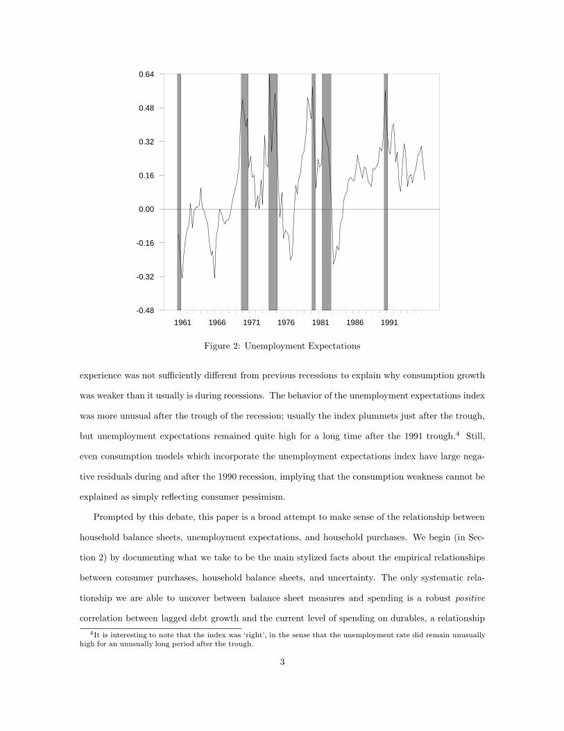
Growth in Total Household LiabilitiesQuarterly Data, 1968:2-1994:3

BalanceSheet

Row/Measure Ht UEt−1 ∆UEt ∆ logAOurst Measure θ SSR D-W

1 0.196 0.539 0.59 2.46(4.64)∗∗∗ (5.85)∗∗∗

2 0.140 −2.169 0.244 0.55 2.15(5.79)∗∗∗ −(5.72)∗∗∗ (2.15)∗∗

3 0.131 −2.864 −1.970 0.306 0.49 2.21(5.78)∗∗∗ −(6.34)∗∗∗ −(3.90)∗∗∗ (2.72)∗∗∗

4 0.133 −2.536 0.180 0.202 0.51 2.12(6.35)∗∗∗ −(7.38)∗∗∗ (3.90)∗∗∗ (1.69)∗

5 0.130 −2.867 −1.662 0.059 0.287 0.49 2.19(5.90)∗∗∗ −(6.41)∗∗∗ −(2.42)∗∗ (0.79) (2.51)∗∗∗

6 ∆ logDt−1 0.045 −1.385 0.588 −0.443 0.48 2.07(2.98)∗∗∗ −(5.25)∗∗∗ (7.84)∗∗∗ −(6.42)∗∗∗

7 rDt−1/Yt−1 0.133 −2.345 0.063 0.218 0.54 2.13(6.12)∗∗∗ −(6.09)∗∗∗ (0.82) (1.86)∗

8 Dt−1/At−1 0.147 −2.063 −0.004 0.259 0.54 2.17(5.85)∗∗∗ −(5.17)∗∗∗ −(0.60) (2.24)∗∗


Notes: t statistics are listed in parentheses below coefficient estimates. Ht is home sales per capita and At is annuity income. UEt−1 isthe unemployment expectations index. The balance sheet variables are the lagged dependent variable (∆ logDt−1), the debt service burden(rDt−1/Yt−1), and the ratio of total household liabilities to annuity income (Dt−1/At−1). θ is the estimated coefficient on the movingaverage error term. A constant term was also included but is not reported.

Table 6: Determinants of Debt Growth

but as in all our previous regressions when a measure of the change in annuity income is added to

the equation the statistical significance of lagged unemployment expectations is unaffected (although

the annuity income growth variable is also significant). Finally, debt growth is uncorrelated with the

lagged values of our other two balance sheet variables but is significantly positively autocorrelated.

These regressions suggest that there is an independent channel for unemployment expectations in

influencing debt growth, even beyond whatever effects unemployment expectations have on home sales.

Because we found earlier that the pace of home sales is itself negatively influenced by unemployment

expectations, in a sense these results imply that unemployment expecatations are doubly important

for debt growth.

Implicit in our entire discussion up to this point has been an assumption that the pattern of debt

over the business cycle is determined by consumers’ unconstrained choices. An alternative possibility

is that debt growth slows over the business cycle not because consumers desire to borrow less but

because lenders restrict credit. A large literature now exists suggesting that lenders tighten credit

standards to businesses during recessions, so that only “high quality” borrowers are able to borrow

15

1981 1984 1987 1990 1993

0.50

0.75

1.00

1.25

1.50

1.75

2.00

2.25

2.50

5

10

15

20

25

30

35

40

45VA_LOANS

ALL_LOANS

Figure 3: VA Originations and Total Mortgage Originations Over Trend GDP

freely in bad times; see Bernanke, Gertler, and Gilchrist (1996) for a survey. A recent paper by

Bernanke, Ferri, and Simon (1997) presents evidence from the Federal Reserve’s Survey of Consumer

Finances suggesting that a similar phenomenon may afflict consumers.

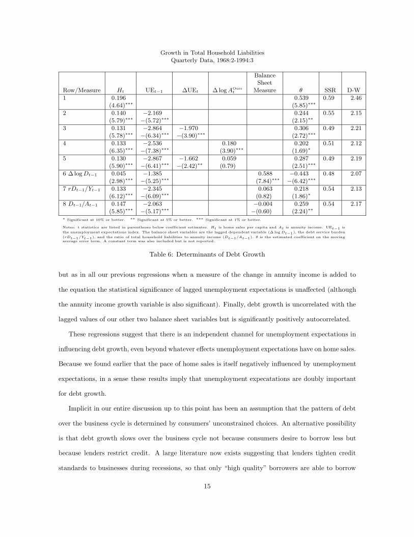
One way to identify demand and supply effects is to examine a form of mortgages for which there

should be no cyclical effect on supply. The best candidate here is mortgages issued by the Veterans’

Administration, because by law these mortgages are available to all qualified former military personnel.

Because the government assumes the default risk, the supply of this form of mortgage financing should

not fluctuate over the cycle even if lenders become more risk-averse in recessions. Indeed, because the

government bears the risk on VA mortgages, one would expect to see a relative increase in the supply

of VA mortgages. If the supply of other forms of credit does decline, we would also expect to see an

increase in the relative demand for VA mortgages; hence any declines in VA mortgage issuance over

the cycle probably underestimate the pure demand effect.

Figure 3 plots the number of VA mortgages originated in each quarter since 1981, together with

total mortgages originated over the same period. There is clearly a strong correlation between VA

16

mortgages and non-VA mortgages. Furthermore, during the two recessions in the sample, VA mort-

gages appear to fall, if anything, by more than non-VA mortgages. This evidence strongly suggests

that demand factors very important role in fluctuations in mortgage borrowing over the business cycle.

This completes our discussion of the cyclical characteristics of consumption spending, home sales,

and household balance sheets. We draw several conclusions. First, spending for nondurables, durables,

and housing all generally respond to changes in annuity income (or at least our measure of annuity

income) in the direction implied by the frictionless CEQ PIH model, although the magnitude of the

response is generally not nearly so large as the model would predict. Second, unemployment expecta-

tions typically seem to play at least as important a role as changes in annuity income in determining

spending decisions. However, most of the information content of unemployment expectations variables

is captured by the lagged level of unemployment expectations rather than by the change in unemploy-

ment expectations. Finally, the only measure of household balance sheet positions that is robustly

correlated with spending appears to be the lagged growth rate of debt.

We turn now to the question of whether a model which incorporates a serious treatment of uncer-

tainty, transactions costs, and liquid assets can explain the broad pattern of our empirical results.

3 The Model

3.1 Theory

The consumer’s objective is to maximize expected discounted utility from consumption of housing

services Z and nonhousing goods C. The period utility function is CRRA in a Cobb-Douglas aggregate

of utility from nonhousing consumption and the stock of housing:

u(Ct, Zt) =(C1−α

t Zαt )1−ρ

(1− ρ) (5)

There are five state variables which constrain or influence the consumer’s choice of C and Z: the

current stock of spendable resources Xt (the sum of wealth and current labor income Yt; or ‘cash-

on-hand’ in Deaton’s (1991) terminology), the size of the home (if any) the consumer owns at the

beginning of the period Hbt ; the level of the consumer’s permanent labor income Pt; an indicator

It for the aggregate state of the economy; and the consumer’s current employment (or Job) status

Jt. Note that we do not list mortgage debt as one of the state variables. This is because we make17

sufficient assumptions to guarantee that the ratio of the mortgage debt to home value is constant,

thereby reducing the number of state variables in the problem by one. The necessary assumption is

that the mortgage payment in each period contains a term that corresponds to the depreciation rate

of the home. Hence the balance owed on the mortgage shrinks in each period by the same fraction

that the value of the home shrinks.

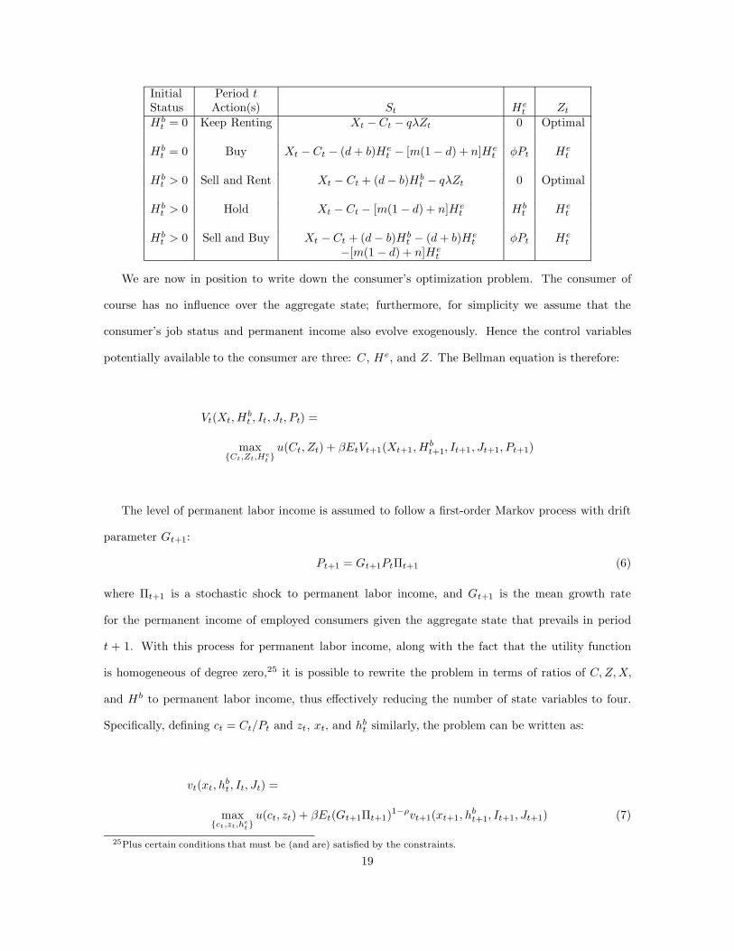
The consumer’s choices within each period are determined as follows (and as summarized in the

table below). First the consumer makes a homeownership decision. If the consumer begins the period

owning no house, Hbt = 0, the decision is whether or not to buy a house whose value we will denote

Het = φPt, i.e. we assume that consumers must by a house whose value is equal to φ = 3 times their

real after-tax permanent income, in accord with standard rules of thumb in the housing industry,

see (1997). Buyers must also put up a down payment of amount d = .2 of the value of the house, and

pay fees and taxes in amount b = .03. Renters purchase housing services in optimally chosen amount

Zt at price qλ where λ is the flow cost of homeownership24 and the restriction q = 1.5 > 1 gives

consumers an incentive to buy. If the consumer begins the period as a homeowner they can sell the

house and rent (implying Het = 0), keep the house they currently own (He

t = Hbt ), or sell the current

house and buy a new one. For homeowners, the flow of housing services is equal to the size of the

house Zt = Het .

Given our assumption that debt depreciates at the same rate as the house, the outstanding amount

of debt will always be given by the amount (1 − d)Hte. We assume that this debt must be serviced

in each period by a fixed mortgage payment m = δ + r where r = .02 is the after-tax real rate of

return and δ = .02 is the depreciation rate of the house. The presence of the δ term in the mortgage

payment represents the lender’s compensation for the erosion in the real value of debt (this term can

be thought of as roughly reflecting inflation).

Denoting the level of liquid assets that the consumer ends the period holding St, we can summarize

the foregoing possibilites in the following table.24Equal to the lost interest on the capital tied up in the house plus depreciation costs plus maintenance costs.

18

Initial Period tStatus Action(s) St He

t ZtHbt = 0 Keep Renting Xt −Ct − qλZt 0 Optimal

Hbt = 0 Buy Xt −Ct − (d+ b)He

t − [m(1− d) + n]Het φPt He

t

Hbt > 0 Sell and Rent Xt − Ct + (d− b)Hb

t − qλZt 0 Optimal

Hbt > 0 Hold Xt − Ct − [m(1− d) + n]He

t Hbt He

t

Hbt > 0 Sell and Buy Xt −Ct + (d− b)Hb

t − (d+ b)Het φPt He

t

−[m(1 − d) + n]Het

We are now in position to write down the consumer’s optimization problem. The consumer of

course has no influence over the aggregate state; furthermore, for simplicity we assume that the

consumer’s job status and permanent income also evolve exogenously. Hence the control variables

potentially available to the consumer are three: C, He, and Z. The Bellman equation is therefore:

Vt(Xt, Hbt , It, Jt, Pt) =

max{Ct,Zt,Het }

u(Ct, Zt) + βEtVt+1(Xt+1, Hbt+1, It+1, Jt+1, Pt+1)

The level of permanent labor income is assumed to follow a first-order Markov process with drift

parameter Gt+1:

Pt+1 = Gt+1PtΠt+1 (6)

where Πt+1 is a stochastic shock to permanent labor income, and Gt+1 is the mean growth rate

for the permanent income of employed consumers given the aggregate state that prevails in period

t + 1. With this process for permanent labor income, along with the fact that the utility function

is homogeneous of degree zero,25 it is possible to rewrite the problem in terms of ratios of C, Z,X,

and Hb to permanent labor income, thus effectively reducing the number of state variables to four.

Specifically, defining ct = Ct/Pt and zt, xt, and hbt similarly, the problem can be written as:

vt(xt, hbt , It, Jt) =

max{ct,zt,het}

u(ct, zt) + βEt(Gt+1Πt+1)1−ρvt+1(xt+1, hbt+1, It+1, Jt+1) (7)

25Plus certain conditions that must be (and are) satisfied by the constraints.

19

We assume that the level of actual labor income in period t is given by the level of permanent

labor income multiplied by a transitory shock Ψt:

Yt = PtΨt (8)

The consumer’s decisions within the period determine the size of the housing stock at the end of the

period Het and the amount of liquid assets (or savings) on hand at the end of the period St subject to

a liquidity constraint that requires St ≥ 0. Given Het and St, the levels of beginning-of-period housing

Hb and cash-on-hand in period t+ 1 are given by:

Hbt+1 = (1− δ)He

t

Xt+1 = RSt + Yt+1

where R = 1.02 is the annual gross interest rate between periods. Dividing both sides of both of

these equations by Pt+1 and substituting from the permanent labor income equation (6) yields:

hbt+1 =het (1− δ)Gt+1Πt+1

xt+1 =R

Gt+1Πt+1st + Ψt+1

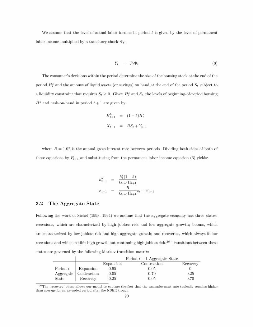
3.2 The Aggregate State

Following the work of Sichel (1993, 1994) we assume that the aggregate economy has three states:

recessions, which are characterized by high jobloss risk and low aggregate growth; booms, which

are characterized by low jobloss risk and high aggregate growth; and recoveries, which always follow

recessions and which exhibit high growth but continuing high jobloss risk.26 Transitions between these

states are governed by the following Markov transition matrix:

Period t+ 1 Aggregate StateExpansion Contraction Recovery

Period t Expansion 0.95 0.05 0Aggregate Contraction 0.05 0.70 0.25State Recovery 0.25 0.05 0.70

26The ‘recovery’ phase allows our model to capture the fact that the unemployment rate typically remains higherthan average for an extended period after the NBER trough.

20

where the switching probabilities were chosen to match the empirical fraction of the time the economy

has spent in expansion versus contraction in the postwar US, and the probabilities for the ‘recovery’

period were chosen so that recoveries would last for four quarters on average, and the probability of

slipping from recovery back into recession is the same as the probability of entering a recession from

an expansion.

3.3 The Household Income Process

3.3.1 The Employment State

Unemployment spells last one or two periods, and when consumers lose their jobs they know whether

the spell will be a one or a two period spell (we chose this structure to allow average spell length to be

longer during recessions than during expansions). Consumers in the last period of an unemployment

spell face the same employment hazards as employed consumers; thus a very unlucky consumer could

experience two (or even more) unemployment spells in a row. Designating status “employed” as E,

unemployed with one remaining quarter of unemployment as U1 and unemployed with two quarters

remaining as quarter as U2 we assume the employment state transition matrix in expansions is:

Period t+ 1 StatusPeriod E U1 U2

t E 0.97 0.01 0.02Status U1 0.97 0.01 0.02

U2 0 1 0

while we assume that in contractions and recoveries the matrix is:

Period t+ 1 StatusPeriod E U1 U2

t E 0.96 0 0.04Status U1 0.96 0 0.04

U2 0 1 0

where the transition probabilities were chosen to generate steady-state unemployment rates around

5 percent in expansions and 8 percent in contractions and recoveries (by “steady-state” we mean

the rate that would eventually prevail if the economy remained in the expansion, or contraction, or

recovery for many periods).

3.3.2 The Transitory Shocks

Transitory shocks to income are drawn for all employed consumers in each period from a three point

symmetric distribution with mean one and equal probability mass on each of the three possible draws.

Thus the possible draws are (1 − νe, 1, 1 + νe) in expansions and (1− νcr, 1, 1 + νcr) in contractions21

and recoveries, νcr ≥ νe (in practice we assume transitory shocks are of equal size in all aggregate

states, νcr = νe = .1). Unemployed consumers receive unemployment compensation in amount YPt

with certainty, where we assume that the replacement rate Y = .5 does not vary with the cycle.

3.4 The Permanent Shocks

For employed consumers, permanent shocks to income, like transitory shocks, are drawn in each

quarter from a three point symmetric distribution with mean one and equal probability mass on each

of the three possible draws. We assume the three possibilities are (0.95, 1.00, 1.05) in all three aggregate

states, which amounts to a conservative estimate given that microeconomic studies typically estimate

that the standard deviation of the annual innovation to permanent income is at least 10 percent

annually (see Carroll (1992) for a brief survey). We assume that unemployment spells in all three

states of the economy typically end with consumers taking jobs at a level of permanent income that is

on average 10 percent lower than the permanent income associated with their previous job (this is one

of the few statistics we were able to calibrate using existing data from the labor economics literature;

see, e.g., Carrington (1993) for evidence on the typical size of wage losses). However, we were unable

to find evidence on how this statistic varies over the business cycle, so we assume that it is the

same in all three aggregate states. We again assume a three point symmetric distribution with equal

probability weights on all three outcomes, but we assume that the shock process during contractions

and recoveries is a mean preserving spread of the shock process during expansions. Specifically, the

possible outcomes are (0.8, 0.9, 1.0) in booms and (0.7, 0.9, 1.1) in contractions and recoveries.

3.5 Summary

Although the model can be solved for quite general combinations of parameter values, we have in-

tentionally kept the structure of uncertainty simple in order to make the model easier to understand

and analyze. In our parameterization, the only differences in risk between aggregate states come from

the fact that in recessions and recoveries unemployment spells are more likely, last longer, and are

associated with larger permanent income shocks. The processes for transitory and permanent shocks

for employed consumers are the same in all three aggregate states, as is the mean of the distribution

for permanent shocks for the unemployed. Many of these parameters could in principle be calibrated

using microeconomic data, but we were not able to find many existing studies that were useful for

22

that purpose.

3.6 A Wish List

In order to solve the model, we had to make a variety of simplifying assumptions. Even so, the full

version of the model used for analysis of the effects of financial market deregulation has six state

variables: the four described above (xt, hbt , It, Jt) plus the current value of the down payment ratio

d required for new home purchases and the value of the down payment ratio that prevailed when the

consumer took out their mortgage loan. The full model takes our new Unix workstation four days

to solve and another two to simulate, so substantially relaxing the simplifying assumptions is not

feasible with present technology. It is nevertheless worthwhile to draw attention to the assumptions

we would most like to relax as technology advances. First is the assumption that the level of debt is

perfectly correlated with the level of the housing stock. We would have preferred to make assumptions

that guaranteed at least a modest buildup of home equity over the course of time. The second

assumption we would like to relax is that there is no house price risk. Although Fratantoni (1996)

found that the effects of this kind of risk were small compared to the effective risk caused by the fixed

mortgage commitment, it would be useful to see whether that result carries over into this context.

This assumption could obviously interact with the first assumption because house price risk could put

some consumers ‘under water,’ holding a mortgage whose value exceeds that of the house. Finally,

we would like to allow consumers to choose the size of the new house they buy. However, we suspect

that this last change would not affect behavior much; because consumers will live in their house for

an average of ten years, it seems unlikely that transitory factors such as the current aggregate state

should optimally have much effect on the optimal size of house to buy.

3.7 Solution

As anyone familiar with the recent literature on consumption under uncertainty would anticipate,

solution of this model was a major challenge. A short companion paper (1997) briefly describes our

solution method, which involves numerical iteration on the value function. Carroll and Kimball (1996)

have shown that even in the simpler case where there is only a single, nondurable, consumption good,

the consumption policy rule is strictly concave (and therefore presumably not analytically soluble)

whenever utility is of the Hyperbolic Absolute Risk Aversion (HARA) form (a class that subsumes

23

Constant Absolute Risk Aversion (CARA), Constant Relative Risk Aversion (CRRA), and Stone-

Geary versions of CARA and CRRA utility) and there is both labor income and rate-of-return risk.

That paper shows that there are only three degenerate cases which yield linear consumption rules:

quadratic utility, Constant Absolute Risk Aversion utility with only labor income risk, and Constant

Relative Risk Aversion with only rate-of-return risk. Given the lack of analytical solutions to even

the simpler problem for nondurable consumption, the resort to numerical methods was inescapable

here - even if the fixed transactions costs did not add major further complications.

Previous work on (S,s) models has either assumed assumed risk neutrality of consumers (Bertola

and Caballero (1990)) or has assumed that the only risk consumers face is rate-of-return risk (Gross-

man and LaRoque (1990), Eberly (1997)) in order to exploit the linearity of the optimal consumption

rule under power utility (which, under certain further assumptions, implies a closed form solution to

even the more complicated (S,s) problem). A very recent paper by Caplin and Leahy (1997) makes

substantial progress in deriving empirical implications of a model in which the marginal utility of

wealth does not vary over the business cycle (except as a result of interest rate fluctuations). While

these assumptions are defensible for many purposes, they are obviously unacceptable in a study of

the effects of labor income uncertainty on durables purchases.

Despite the mathematical difficulty of solving the model, the behavior of consumers in this model

can be described reasonably simply. Most of the time they are homeowners, because ownership is

cheaper than renting. During most of the time that they are homeowners, they engage in “buffer-

stock saving,” in which they try to maintain a target level of liquid precautionary assets which they use

to smooth nonhousing consumption in the face of income shocks (see Deaton (1991) and Carroll (1992,

1997) for detailed analysis of buffer-stock saving behavior in a model with only nondurable goods).

As the time approaches to buy a new home, however, they engage in a bit of extra saving in order to

accumulate the required downpayment.

The homeownership decision can be described as following a modified (S,s) rule. Because the value

of the house depreciates over time, and because permanent labor income grows, the ratio of home value

to permanent labor income drifts down over time. When this ratio drops far enough the consumer

sells the existing home and buys a new one. The most important twist in this model, relative to

the standard (S,s) model of durable goods, is that the precise trigger point at which the consumer

24

3.5 4.0 4.5 5.0 5.5 6.0Cash On Hand

6.4

6.6

6.8

7.0

7.2

7.4

Trigger

<- Contraction

Expansion ->

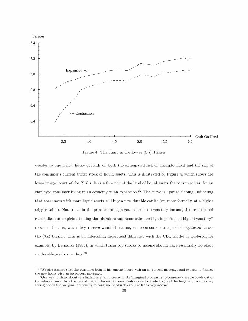
Figure 4: The Jump in the Lower (S,s) Trigger

decides to buy a new house depends on both the anticipated risk of unemployment and the size of

the consumer’s current buffer stock of liquid assets. This is illustrated by Figure 4, which shows the

lower trigger point of the (S,s) rule as a function of the level of liquid assets the consumer has, for an

employed consumer living in an economy in an expansion.27 The curve is upward sloping, indicating

that consumers with more liquid assets will buy a new durable earlier (or, more formally, at a higher

trigger value). Note that, in the presence of aggregate shocks to transitory income, this result could

rationalize our empirical finding that durables and home sales are high in periods of high “transitory”

income. That is, when they receive windfall income, some consumers are pushed rightward across

the (S,s) barrier. This is an interesting theoretical difference with the CEQ model as explored, for

example, by Bernanke (1985), in which transitory shocks to income should have essentially no effect

on durable goods spending.28

27We also assume that the consumer bought his current house with an 80 percent mortgage and expects to financethe new house with an 80 percent mortgage.

28One way to think about this finding is as an increase in the ‘marginal propensity to consume’ durable goods out oftransitory income. As a theoretical matter, this result corresponds closely to Kimball’s (1990) finding that precautionarysaving boosts the marginal propensity to consume nondurables out of transitory income.

25

The figure also shows (the dashing line) how the trigger locus changes if the economy enters a

recession: for any given level of liquid assets, the trigger point is lower (consumers will put up with

living in a poorer house rather than buy). That is, a consumer who had been on the brink of home

purchase before the economy entered the recession will now wait until the house has depreciated

more before buying. Alternatively, a consumer with a given house value will require a larger stock

of precautionary liquid assets before he will be willing to buy. This shift in the lower (S,s) trigger is

what we refer to in the title of the paper as “Jumping (S,s) Triggers.”

The foregoing story is somewhat different from the standard (S,s) model’s explanation of durables

purchases over the business cycle found in, for example, Bar-Ilan and Blinder (1992) or Bertola and

Caballero (1990) or Caplin and Leahy (1997).29 The main difference is the explicit importance of

cyclical variation in labor income uncertainty in our model; in the standard model, the sharp drop in

durables purchases in recessions is triggered, not by an increase in uncertainty, but by a decrease in

the level of expected future income and thus of ‘permanent income’ as they define it. The empirical

distinction between the two models is thus that our model would imply a strong effect of uncertainty

per se on durables purchases, even after controlling for permanent (or annuity) income. Another way

to interpret the jump in the trigger is as reflecting the fact that an increase in uncertainty causes an

increase in the marginal utility of liquid wealth, because its value as a buffer-stock against uncertainty

rises. This is in explicit contrast with Caplin and Leahy’s assumption that the marginal utility of

wealth is constant.30

For purposes of cyclical anlaysis, the most important implication of the model comes from the

interaction of the precautionary saving motive and the jumping (S,s) bands. When the economy

switches into a recession, a large proportion of the entire set of consumers who had been on the brink

of home purchase suddenly feel that their current stock of precautionary saving, which had been

adequate when they anticipated continued prosperity, is inadequate in the new, riskier environment.

These consumers postpone their home purchases until they have accumulated enough additional pre-29One interesting recent paper that adopts a rather different approach to these issues is Greenspan and Cohen (1997),

who model vehicle sales as a function of “scrappage” and who make a distinction between “engineering scrappage” and“cyclical scrappage.” Roughly speaking, however, it is possible to interpret the effects of the jumping (S,s) trigger inour model as corresponding to the “cyclical scrappage” term in the Greenspan and Cohen model.

30One recent paper which focuses on the effects of jumping (S,s) triggers is Adda and Cooper (1997), who examinethe effects of two natural experiments thoughtfully provided to economists by the French government. The experimentsinvolved subsidies to automobile scrappage, which should have had the effect of moving the lower (S,s) trigger up. Addaand Cooper document that the reaction of automobile sales to the tax subsidies was quite similar to the predictions ofan (S,s) model when the lower trigger moves up.

26

cautionary savings to again feel comfortable with the home purchase decision (or until their home has

deteriorated so much that they are willing to risk buying a new one even with a low buffer-stock of

liquid assets).31

Another interesting feature of this model that is not present in the standard model is that home

equity serves as an additional reserve of emergency precautionary resources beyond liquid assets.

Consumers who experience a particularly vicious series of income shocks can, in the last resort,

sell their houses in order to tap the equity to finance current consumption. Of course, they pay a

heavy price for this; they must incur brokerage fees and pay for rented housing services at a price

substantially higher than the user cost of ownership. Still, extreme circumstances call for extreme

measures. This feature of the model is interesting because several papers in the empirical literature

on precautionary saving have found larger effects of uncertainty on net worth than on liquid assets.

Carroll and Samwick (1997) speculate that the reason may be precisely this potential use of home

equity as a precautionary reserve.

Our paper is not the first to argue that variations in the degree of uncertainty are important in

explaining durables purchases over the business cycle. As Bernanke (1983) pointed out, and many

authors have emphasized since, an increase in uncertainty increases the ‘option value’ of waiting until

the uncertainty is resolved.32 A formal illustration of this can be seen in Eberly (1997); she shows

that in a model with only rate-of-return risk, when the degree of rate-of-return risk goes up the

(S,s) bands widen, provoking a response similar to that of the jump in the (S,s) band we depict.

However, the underlying cause of the jump is rather different. In Eberly’s model the primary reason

for the shift in the (S,s) bands is that if the bands did not change, an increase in uncertainty would

increase the expected present discounted value of the adjustment costs the consumer would have to

pay. Thus the effect of uncertainty in her model has little to do with precautionary behavior - instead,

it mainly reflects a change in the tradeoff between minimizing average fixed costs and minimizing

average distance from the optimal housing stock. Again, a useful way to understand the difference

between the models is to realize that the main effect driving the jump in the (S,s) trigger in our model31In the Greenspan/Cohen model, the implication would be that “cyclical scrappage” is strongly related to unemploy-

ment expectations. Although Greenspan and Cohen do not report regressions of cyclical scrappage on unemploymentexpectations, they do report that cyclical scrappage falls when the unemployment rate rises, which is roughly what onewould expect from our model.

32For a thorough and recent treatment, see Dixit and Pindyck (1994).

27

is an increase in the marginal utility of liquid assets - an effect that is absent in the Bernanke and

Eberly models.

An even earlier analysis of many of these issues can be found in three insightful articles by Frederick

Mishkin (1977, 1976, 1978) which anticipate many (though not all) of the theoretical results that come

from our formal optimizing model. In particular, Mishkin (1978) argues that “A consumer suffering

financial distress, and unable to pay his bills readily, would prefer holding highly liquid financial

assets. This implies that as the consumer perceives an increasing probability of financial distress,

he will decrease his demand for consumer durables and limit his purchases.” Using an intuitive but

ad-hoc functional form, Mishkin also documents a strong correlation between durables purchases and

consumer sentiment, and explicitly interprets consumer sentiment as a measure of uncertainty.

4 Simulation Results

4.0.1 A Stylized Business Cycle

Our simulation results examine the aggregate characteristics of an economy populated by 20,000

consumers behaving according to the optimal decision rules that solve the maximization problem

in Section 3. As preparation for the simulations, we start the model economy off at an essentially

arbitrary point, then simulate for 400 quarters of expansion, by which time it has settled into a

stochastic steady-state with a reasonably settled distribution of consumers across the state space.

The first experiment we perform is to examine a recession of typical length (four quarters) followed

by recovery period of the same length. We show the path of aggregate variables from 8 quarters before

the beginning of the recession to four quarters after the end of the recovery. Results are shown in

Figures 5 and 6; the contraction is shaded dark gray and the recovery period is shaded light gray.

In the first quarter of the recession, the unemployment rate begins moving up as the new, higher job

loss risk affects its first batch of victims. Recall, however, that unemployment spells in recessions last

two quarters; this means that the new recessionary equilibrium level of the unemployment rate is only

reached in the second quarter of recession. Thereafter the unemployment rate stays at the same high

level throughout the recession and recovery periods, reverting to its expansionary level only in the

second quarter after the end of the recovery period.

The adjacent chart shows the expected risk of job loss over the next four quarters for a currently

28

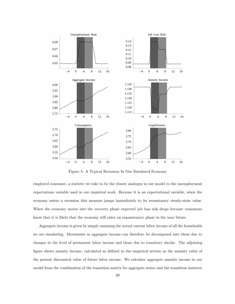
-4 0 4 8 12 163.50

3.55

3.60

3.65

3.70

3.75Consumption

-4 0 4 8 12 163.55

3.60

3.65

3.70

3.75

3.80

LiquidAssets

-4 0 4 8 12 163.75

3.80

3.85

3.90

3.95

4.00

Aggregate Income

-4 0 4 8 12 16

1.115

1.120

1.125

1.130

1.135

1.140

1.145

Annuity Income

-4 0 4 8 12 16

0.05

0.06

0.07

0.08

Unemployment Rate

-4 0 4 8 12 16

0.08

0.09

0.10

0.11

0.12

0.13

0.14

Job Loss Risk

Figure 5: A Typical Recession In Our Simulated Economy

employed consumer, a statistic we take to be the closest analogue in our model to the unemployment

expectations variable used in our empirical work. Because it is an expectational variable, when the

economy enters a recession this measure jumps immediately to its recessionary steady-state value.

When the economy moves into the recovery phase expected job loss risk drops because consumers

know that it is likely that the economy will enter an expansionary phase in the near future.

Aggregate income is given by simply summing the actual current labor income of all the households

we are simulating. Movements in aggregate income can therefore be decomposed into those due to

changes in the level of permanent labor income and those due to transitory shocks. The adjoining

figure shows annuity income, calculated as defined in the empirical section as the annuity value of

the present discounted value of future labor income. We calculate aggregate annuity income in our

model from the combination of the transition matrix for aggregate states and the transition matrices

29

for employment states during each aggregate state. In calculating annuity income we abstract from

the long-term secular growth in income; results would have been essentially the same had we allowed

the drift term to enter.

Nondurables consumption, which is determined (as always) in large part by expectations, drops

immediately and sharply when the economy enters a recession. Consumption recovers somewhat when

the economy enters the recovery phase and further when the economy enters the expansionary phase.

The final figure in the set shows the behavior of liquid assets, which rise sharply during the recession

because households feel the need to boost the level of their precautionary buffer-stocks. Note that

the precautionary motive is intense enough to outweigh the dissaving being done by the unemployed

consumers. Savings level off during the recovery period and remain flat when the expansion begins.

The next set of figures shows the evolution of the housing market and household balance sheets.

In the first two quarters of the recession, home sales plummet for the reasons described above: newly

wary consumers want a higher level of precautionary liquid assets before buying a house. Note the

impressive magnitude of the initial decline in home sales: the rate of sales per capita falls by roughly

50 percent. After the initial collapse, home sales begin to rise again, then show a minor surge when

the economy enters the recovery phase. Finally, when the economy switches into expansion there is a

massive surge of home sales as the consumers who had been postponing purchases for precautionary

reasons throw caution to the wind.

This last phenomenon, the surge of sales when the economy exits the contraction, has a natural

interpretation as the release of “pent-up demand.” “Pent-up demand” is a phrase used loosely by

analysts of the housing and auto sectors who claim that recessions are periods when “pent-up demand”

rises, only to be ‘released’ when the economy emerges from the contraction. Pent-up demand could be

defined rigorously in our model as the demand which would be immediately be expressed in purchases

if consumer expectations returned to normal levels. In other words, pent-up demand corresponds to

the set of consumers populating the region of the (S,s) diagram between the jumping loci of the lower

(S,s) band.33

It is worth noting just how close the correspondence is between this phenomenon in the formal33This definition differs somewhat from the definition proposed by Caballero and Engel (1994). They investigate

a model with fixed (S,s) bands and describe a period of high pent-up demand as a period with a heavier than usualconcentration of agents near the (unmoving) trigger point.

30

-4 0 4 8 12 16

0.0725

0.0730

0.0735

0.0740

0.0745

Debt Service Burden

-4 0 4 8 12 16

6.30

6.35

6.40

6.45

6.50

Debt Over Annuity Income

-4 0 4 8 12 160.000

0.002

0.004

0.006

0.008

0.010

0.012

Debt Growth

-4 0 4 8 12 165.75

5.80

5.85

5.90

5.95

6.00

Debt

-4 0 4 8 12 16

0.010

0.015

0.020

0.025

Home Purchases

-4 0 4 8 12 16

6.00

6.05

6.10

6.15

6.20

6.25Housing Stock

Figure 6: The Housing Market and Balance Sheets

model and the informal descriptions of industry analysts in both the housing and the automotive

markets. For example, a May 11, 1992 editorial (p. 12) in Automotive News read, in part: “[F]olks

still aren’t buying cars . . . and I am convinced that most Americans are still concerned about their

jobs. As long as that insecurity exists, we are going to see a sluggish auto industry.”

The figure adjacent to the home sales figure shows the obvious implication of sales for the level of

the housing stock: at the onset of a recession, the growth rate of the housing stock decelerates. Below

are the growth rate of debt and the time path of the debt stock, which strongly resemble the patterns

of home purchases and the housing stock.

The final two figures show the behavior of our measures of household balance sheet conditions

over the business cycle. Both the debt service burden and the ratio of debt to annuity income rise

sharply at the beginning of the recession, in both cases because the numerator is largely fixed by past

31

decisions while the denominator (income or annuity income) falls when the economy enters a recession.

Thereafter the debt service burden drifts until the economy enters a full expansionary phase again,

while the ratio of debt to annuity income drops as soon as the economy enters the recovery period

(because the level of annuity income jumps up; see the previous set of figures).

5 Comparing the Model to US Cyclical Data

We turn now to some simulations based on the pattern of expansion and contraction for the US

economy since 1961, roughly the period for which we were able to perform our empirical work on

US NIPA data. Again we start the economy off from the steady-state equilibrium achieved after

400 quarters of continuous expansion, but for quarters 401 through 539 (corresponding to 1962Q2

through 1995Q4) we set the aggregate state of the simulated economy equal to the aggregate state

of the corresponding quarter for the US economy as indicated by the official NBER chronology. (We

arbitrarily assume that every recession is followed by a recovery period that is four quarters long,

which is the expected duration implied by the transition matrix.) The next set of figures shows the

results graphically.

32

1961 q2 1995 q4-0.03

-0.02

-0.01

0.00

0.01

0.02

0.03Consumption Growth

1961 q2 1995 q4

0.775

0.800

0.825

0.850

0.875

0.900

0.925LiquidAssets Over Perm. Income

1961 q2 1995 q4

-0.010-0.005

0.0000.0050.0100.0150.0200.025

Income Growth

1961 q2 1995 q4

1.115

1.120

1.125

1.130

1.135

1.140

1.145

Annuity Income

1961 q2 1995 q4

0.05

0.06

0.07

0.08

Unemployment Rate

1961 q2 1995 q4

0.08

0.09

0.10

0.11

0.12

0.13

0.14

Job Loss Risk

Figure 7: Simulated Economy with Actual Recession Pattern

33

1961 q2 1995 q4

0.0725

0.0730

0.0735

0.0740

0.0745

0.0750

0.0755Debt Service Burden

1961 q2 1995 q4

6.30

6.35

6.40

6.45

6.50

6.55

6.60Debt Over Annuity Income

1961 q2 1995 q4

0.000

0.005

0.010

0.015

Debt Growth

1961 q2 1995 q47.15

7.20

7.25

7.30

7.35

Debt Over Perm. Income

1961 q2 1995 q40.005

0.010

0.015

0.020

0.025

0.030Home Purchases

1961 q2 1995 q4

8.95

9.00

9.05

9.10

9.15

9.20

Housing Stock Over Perm. Income

Figure 8: Housing, Debt, and Balance Sheets

34

5.1 Nondurables Consumption Growth

We begin by examining the analogue to the Campbell-Mankiw equation estimated in the first part of

the paper. The top panel of Table 7 reproduces the baseline sentiment-augmented Campbell-Mankiw

equation from Table 1. The first row of the second panel of the table shows that when a standard

Campbell-Mankiw equation is estimated on the simulated nondurables consumption data from our

model, the forecastable component of income growth gets an insignificant and negative coefficient.34

The second row shows that consumption growth is not significantly related to lagged unemployment

expectations, again in accord with the CEQ PIH model and at variance iwth the empirical results.

Finally, when both predictable income growth and lagged unemployment expectations are included,

neither is significant at the 5 percent level. Thus, under baseline parameter values the model does not

reproduce the empirical results we found when estimating the Campbell-Mankiw model in Table 1.

The next regressions examine the model’s predictions for the explanatory power of lagged balance

sheet measures. In accord with our empirical results, none of the balance sheet measures has any

explantory power for nondurables consumption growth.

The next table examines how nondurables consumption in our model responds to innovations to

income and unemployment expectations; the corresponding US empirical results from Table 2 are

again reproduced in the top panel. Recall that the CEQ PIH model would imply a coefficient of 1

on ∆ logAt and zero on all other variables, while the Campbell-Mankiw model with λ = .5 would

imply coefficients of 0.5 on both ∆ logYt and ∆ logAt, but would still imply coefficients of zero on

the UE variables. Row 3 of the second panel shows that under baseline parameter values our model

implies a coefficient of about 0.49 on ∆ logYt and 0.59 on ∆ logAt. Both of these coefficients larger

than the values estimated in the empirical data (row 0). However, the major difference between our

model and either the CEQ PIH model or the Campbell-Mankiw model is our model’s implication

that both the lagged level and the change in UE should be highly statistically significant.35 This

constitites at least a partial victory relative to the standard models which provide no role at all for

unemployment expectations per se. However, it is fair to say that the model is at best a modest34Under some alternative parametric assumptions the model does reproduce the Campbell-Mankiw finding. Given

how long it takes to solve the model, we were unable to explore the parameter space sufficiently to determine whatkinds of parametric combinations generate the Campbell-Mankiw result.

35Because the variables are defined rather differently, and scaled quite differently, it would not be appropriate tocompare the coefficient estimates on UE from the model to those from the data; hence we examine only statisticalsignificance.

35

Nondurable Consumption GrowthSimulation Data

BalanceRow/Measure Et−1∆ logYt UEt−1 Sheet SSR D-W

Empirical Results (reproduced from Table 1)0 0.269 −0.906 0.50 1.98

(1.64) −(2.18)∗∗

Simulations Under Baseline Parameter Values1 0.032 0.55 1.93

(0.19)2 0.404 0.55 1.81

(1.45)3 0.244 0.633 0.47 1.97

(1.31) (2.03)∗∗

4 ∆ logDt−1 0.417 0.507 −0.394 0.42 1.98(1.92)∗ (1.61) −(1.29)

5 rDt−1/Yt−1 0.182 0.459 0.359 0.49 1.97(0.78) (0.98) (0.54)

6 Dt−1/At−1 0.229 0.495 0.007 0.47 1.97(1.21) (1.25) (0.57)

Simulations After Financial Liberalization7 −0.127 0.73 1.96

−(0.62)8 0.572 0.67 1.93

(1.87)∗

9 0.135 0.698 0.62 2.00(0.58) (1.90)∗


Notes: t Statistics are listed in parentheses below coefficient estimates. Yt is total household wage andtransfer income. UEt−1 is the unemployment expectations index. The instruments are the same as thoseused in Carroll, Fuhrer, and Wilcox (1994). The balance sheet variables are the growth in total householdliabilities (∆ logDt−1), the debt service burden (rDt−1/Yt−1), and the ratio of total household liabilitiesto annuity income (Dt−1/At−1). A constant term was also included but is not reported.

Table 7: The Campbell-Mankiw Model Estimated on Simulated Data

success in explaining nondurables data, since it does not replicate the basic Campbell-Mankiw result.

Furthermore, even for the unemployment expecataions variable the match between theory and data is

imperfect: the theory implies that the contemporaneous change in unemployment expectations should

be vastly more important than the lagged level, but the empirical regressions found the opposite result.

Carroll, Fuhrer, and Wilcox (1994) speculate that a model which incorporates both habit formation

and labor income uncertainty might be able to explain the importance of lagged uncertainty for

current consumption growth; a recent paper by Overland (1997) provides a formal underpinning for

36

Nondurable Consumption GrowthSimulation Data

Row ∆ logYt ∆ logAt UEt−1 ∆UEt R2

D-W

Empirical Results (reproduced from Table 2)0 0.324 0.124 −1.003 −0.907 0.34 1.92

(3.15)∗∗∗ (1.59) −(2.93)∗∗∗ −(1.52)

Simulations Under Baseline Parameters1 0.109 1.323 −3.398 0.86 2.44

(1.51) (22.41)∗∗∗ −(2.41)∗∗

2 0.078 −4.470 −5.561 0.95 1.86(1.85)∗ −(5.43)∗∗∗ −(41.28)∗∗∗

3 −0.006 0.486 −5.860 −4.050 0.98 1.62−(0.21) (12.08)∗∗∗ −(10.07)∗∗∗ −(25.94)∗∗∗

Simulations After Financial Liberalization4 −0.032 1.530 −4.394 0.86 2.50

−(0.36) (21.85)∗∗∗ −(2.67)∗∗∗

5 −0.054 −5.434 −63.926 0.95 1.76−(1.05) −(5.56)∗∗∗ −(39.55)∗∗∗

6 −0.186 0.596 −7.510 −46.023 0.98 1.57−(5.36)∗∗∗ (13.75)∗∗∗ −(11.59)∗∗∗ −(27.59)∗∗∗


Notes: t statistics are listed in parentheses below coefficient estimates. Standard errors were constructed usinga serial correlation-robust covariance matrix (allowing serial correlation at lags up to 8). Yt is total householdwage and transfer income. At is annuity labor income. UEt−1 is the unemployment expectations index. Aconstant term was also included but is not reported.

Table 8: Effect of Innovations on Nondurables Consumption

37

this idea. Alternatively, it may take consumers time to formulate new spending plans upon receipt

of new information; this could be formalized in a model in which consumers draw up budgets only

periodically, and do not change their spending patterns until they find the time to draw up a new

budget.

5.2 The Cyclical Dynamics of Durables Spending

Table 9 presents the results when we estimate equations for our simulated home sales data similar to

those estimated earlier for both NIPA durable goods and total US home sales; again the corresponding

empirical result is reproduced in the first row of the table.36

In our simulated data the annuity income ratio is insignificant but both the lagged level of un-

employment expectations and the change in unemployment expectations are highly significant. Here

the level and the change in the level of the unemployment expectations index are roughly equally

statistically significant.

Turning to the balance sheet variables, lagged debt growth receives a positive and significant

coefficient; recall that it was the only balance sheet variable that was robustly significant in the NIPA

data. Although simultaneity seemed the most plausible interpretation for the empirical results there

was no obvious way to prove that simultaneity was the correct interpretation. Here the answer is clear:

simultaneity is the culprit. Debt growth is acting as a statistic for all of those characteristics of the

aggregate environment which are important in determining the pace of home sales but are not captured

by the other observed aggregate variables. For example, during the course of recessions home sales

and debt growth both plummet initially, but recover substantially over the succeeding few quarters

(even while the economy remains in recession). The partial recovery in sales reflects a combination of

the buildup of consumers’ buffer-stocks of precautionary savings and the continuing depreciation of

their homes (moving some of them across even a lowered (S,s) trigger). These changing circumstances

are not captured by our observed aggregate variables, but they are at least partly captured by lagged

debt growth. Hence lagged debt growth’s statistical significance is entirely attributable to the fact

that it is an endogenous variable responding to unobserved but important real determinants of home36Here we take the “corresponding” result from the table on durable goods spending rather than the table on home

sales. Although we calibrate our model to match certain features of the housing market, it is clear that under alternativeparameter values the model could equally be interpreted as a model of purchases of automobiles or other durable goods.Given the similarity of the empirical results for home sales and durable good sales documented in Tables 3 and 5, it isof little consequence whether we compare our model’s predictions to the pattern of durable goods sales or home sales.

38

Home SalesSimulated Data

BalanceSheet

Row/Measure At−1/At UEt−1 ∆UEt Yt/At Measure R2

D-W

Empirical Baseline (reproduced from Table 5)0 −0.542 −7.471 −1.541 1.172 0.51 0.33

−(3.48)∗∗∗ −(4.21)∗∗∗ −(0.70) (2.99)∗∗∗

Simulations Under Baseline Parameters1 0.037 −5.260 −19.407 −0.106 0.76 1.80

(0.85) −(8.07)∗∗∗ −(10.55)∗∗∗ −(2.57)∗∗∗

2 ∆ logDt−1 0.048 −4.047 −20.452 −0.081 0.179 0.77 2.16(1.14) −(5.50)∗∗∗ −(11.31)∗∗∗ −(1.98)∗∗ (3.20)∗∗∗

3 rDt−1/Yt−1 0.043 −5.780 −19.641 −0.100 0.154 0.76 1.79(0.98) −(7.63)∗∗∗ −(10.66)∗∗∗ −(2.41)∗∗ (1.33)

4 Dt−1/At−1 0.026 −4.875 −19.227 −0.096 −0.002 0.76 1.79(0.57) −(5.49)∗∗∗ −(10.31)∗∗∗ −(2.16)∗∗ −(0.64)

Simulations After Financial Liberalization5 −0.189 −7.020 −21.149 −0.296 0.80 1.93

−(2.71)∗∗∗ −(6.67)∗∗∗ −(6.74)∗∗∗ −(4.56)∗∗∗∗ Significant at 10% or better. ∗∗ Significant at 5% or better. ∗∗∗ Significant at 1% or better.

Notes: t statistics are listed in parentheses below coefficient estimates. At is annuity labor income and Yt is total household wage and transferincome. UEt−1 is the unemployment expectations index. The balance sheet variables are the growth in total household liabilities (∆ logDt−1),the debt service burden (rDt−1/Yt−1), and the ratio of total household liabilities to annuity income (Dt−1/At−1). A constant term was alsoincluded but is not reported.

Table 9: Home Sales in the Simulated Economy

sales.

The remainder of Table 9 shows that the other two lagged balance sheet variables are not system-

atically related to home sales (as they were not in the empirical data). The reason can be seen in

Figure 8: the debt to income ratio and the debt service burden tend to be high during recessions be-

cause income is temporarily low, but also tend to be high in recoveries and early expansions, because

upon recovery the pent-up demand built up during the recession is satisfied by a large number of home

purchases and a consequent runup in aggregate debt. Hence both variables tend to be higher than

average both during periods of particularly low sales (recessions) and particularly high sales (early

recoveries and expansions).

The fundamental question these regressions are designed to address is whether our model performs

better than the standard models in explaining our empirical findings in Tables 3, 4 and 5. On the

whole, the answer is yes. Our model implies a very important role for unemployment expectations

39

beyond any correlation they may have with current or expected future levels of income. And it

provides an interpretation for the finding that lagged debt growth is consistently positively related to

current home sales and that other balance sheet measures are not consistently related to home sales.

However, as in the nondurables regressions, the model implies a much stronger reaction to innovations

in uncertainty than we observe empirically. We speculated above that habit formation might explain

the sluggishness of nondurables consumption with respect to unemployment expectations innovations;

for durable goods, however, time-to-build or decision lag considerations seem more plausible. This is

especially so for housing decisions; a consumer who has gone to the trouble of house-hunting, lining

up financing, negotiating and bidding on a house is unlikely to back out at the last moment because

of a sudden change in unemployment expectations. Similar but less forceful arguments apply for

automobile purchases.

5.3 The Cyclical Dynamics of Debt Growth

In the model, the primary determinant of debt growth is home sales. Indeed, since all debt is used

for home purchases, and since the value of all homes purchased is in exactly the same proportion to

the permanent labor income of the buyer, one might think that the model implies that data on home

sales should explain 100 percent of the variation on debt growth. A glance at figure 6 will confirm

that the patterns of home sales and debt growth over the cycle are indeed quite similar. However, the

model does provide several channels through which other variables influence aggregate debt growth.

First, a small number of consumers who have experienced a particularly nasty series of shocks find

themselves forced to sell their homes and rent temporarily in order to get access to the emergency

reseve of precautionary resources represented by their home equity. Second, among the consumers

who are currently renting, fewer will be willing to buy new homes when unemployment expectations

are pessimistic. The number of consumers who are forced to sell and rent will obviously be on average

related to the level and change of unemployment expectations. Finally, note that the fact that the

(S,s) trigger jumps around means that even though every purchase represents exactly the same amount

of debt acquisition (relative to the permanent income of the buyer), every sale does not reflect the

same amount of debt retired. Hence we should expect variables that affect the location (S,s) trigger

to have an effect on debt growth.

40

Growth in Total Household LiabilitiesSimulated Data

BalanceSheet

Row/Measure Ht UEt−1 ∆UEt ∆ logAt Measure R2

D-W

Empirical Baseline (reproduced from Table 6)0 0.130 −2.867 −1.662 0.059 2.12

(5.90)∗∗∗ −(6.41)∗∗∗ −(2.42)∗∗ (0.79)

Simulations Under Baseline Parameters1 0.826 0.76 2.07

(20.95)∗∗∗

2 0.812 −1.419 0.77 2.22(20.88)∗∗∗ −(2.81)∗∗∗

3 0.805 −1.465 −0.203 0.77 2.22(10.36)∗∗∗ −(2.24)∗∗ −(0.11)

4 0.791 −1.564 0.017 0.77 2.23(13.54)∗∗∗ −(2.67)∗∗∗ (0.49)

5 0.806 −1.477 0.726 0.026 0.77 2.24(10.34)∗∗∗ −(2.25)∗∗ (0.30) (0.56)

6 ∆ logDt−1 0.826 −2.324 −0.126 0.78 1.94(21.43)∗∗∗ −(3.79)∗∗∗ −(2.51)∗∗∗

7 rDt−1/Yt−1 0.825 −0.673 −0.223 0.78 2.20(21.25)∗∗∗ −(1.11) −(2.17)∗∗

8 Dt−1/At−1 0.811 −0.916 −0.003 0.77 2.21(20.88)∗∗∗ −(1.41) −(1.23)


Notes: t statistics are listed in parentheses below coefficient estimates. Ht is home sales per capita. UEt−1 is the unemployment expectationsindex. The balance sheet variables are the lagged dependent variable (∆ logDt−1), the debt service burden (rDt−1/Yt−1), and the ratioof total household liabilities to annuity income (Dt−1/At−1). A constant term was also included but is not reported.

Table 10: Debt Growth and its Correlates

Table 10 presents the results when we estimate regressions for debt growth like those estimated in

Table 6 above. As expected (and as in the empirical data), debt growth is very closely related to home

sales; when the pace of home sales is the only regressor, the R2

is 0.76. However, the next regression

shows that the lagged level of the unemployment expectations index does provide additional explana-

tory power for debt growth (again corresponding to the empirical result). When we add the growth

rate of annuity income to this baseline regression, the innovation to annuity income is not statistically

significant, in contrast with the empirical regressions. In contrast to the results for durable and non-

durable goods, the change in unemployment expectations is not statistically significant. Finally, we

consider the lagged balance sheet measures, all of which are negatively correlated with current debt

growth. These results contrast with the empirical regressions, in which the lagged dependent variable

41

received a strongly positive coefficient and the other balance sheet measures were insignificant.

In sum, the model captures (almost by assumption) the strong empirical correlation between

home sales and debt growth, but, in contrast with a CEQ PIH model or a standard (S,s) model it also

provides an interpretation for the emprical finding that unemployment expectations are significantly

related to debt growth. It does not, however, imply the observed empirical positive autocorrelation

in debt growth after unemployment expectations have been controlled for.

5.4 Summary

The analysis of this section has attempted to determine whether our model does a better job than

standard models of explaining the empirical regularities relating nondurable consumption growth,

durables purchases, and balance sheet variables. The model is successful in that it implies an important

role for unemployment expectations in addition to the expected level of future income. However,

it also suggests that there is a paradox about the role of unemployment expectations: while the

model implies that consumption growth, durables purchases, and debt acquisition should be strongly

affected by changes in unemployment expectations, our empirical work found that the lagged level of

expectations was always much more statistically important than the change in expectations.

6 Was the 1990 Recession “Special”?

To this point in the paper we have not directly addressed the question of whether the 1990 recession

was “special” in any sense, although we motivated the paper by noting that common analyses of the

1990 recession attributed the unusual consumption weakness to ‘household debt overhang.’ In this

section we examine first the theory and then the evidence.

6.1 Theory

6.1.1 The Dynamic Response to Deregulation

As briefly noted earlier, prior to the 1990 recession there was a rapid and considerable runup in the

ratio of household debt to income (see Figure 1). The most plausible explanation is that this was the

consequence of the wide-ranging deregulation of financial markets that took place in the late 1970s

and early 1980s.

Capturing the full complexity of financial deregulation is obviously beyond the scope of the model

42

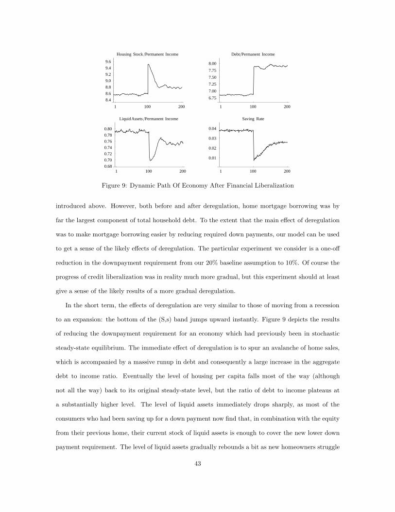
1 100 2000.68

0.70

0.72

0.74

0.76

0.78

0.80

LiquidAssets �Permanent Income

1 100 200

0.01

0.02

0.03

0.04

Saving Rate

1 100 200

8.4

8.6

8.8

9.0

9.2

9.4

9.6

Housing Stock �Permanent Income

1 100 200

6.75

7.00

7.25

7.50

7.75

8.00

Debt�Permanent Income

Figure 9: Dynamic Path Of Economy After Financial Liberalization

introduced above. However, both before and after deregulation, home mortgage borrowing was by

far the largest component of total household debt. To the extent that the main effect of deregulation

was to make mortgage borrowing easier by reducing required down payments, our model can be used

to get a sense of the likely effects of deregulation. The particular experiment we consider is a one-off

reduction in the downpayment requirement from our 20% baseline assumption to 10%. Of course the

progress of credit liberalization was in reality much more gradual, but this experiment should at least

give a sense of the likely results of a more gradual deregulation.

In the short term, the effects of deregulation are very similar to those of moving from a recession

to an expansion: the bottom of the (S,s) band jumps upward instantly. Figure 9 depicts the results

of reducing the downpayment requirement for an economy which had previously been in stochastic

steady-state equilibrium. The immediate effect of deregulation is to spur an avalanche of home sales,

which is accompanied by a massive runup in debt and consequently a large increase in the aggregate

debt to income ratio. Eventually the level of housing per capita falls most of the way (although

not all the way) back to its original steady-state level, but the ratio of debt to income plateaus at

a substantially higher level. The level of liquid assets immediately drops sharply, as most of the

consumers who had been saving up for a down payment now find that, in combination with the equity

from their previous home, their current stock of liquid assets is enough to cover the new lower down

payment requirement. The level of liquid assets gradually rebounds a bit as new homeowners struggle

43

to build up their buffer-stocks of liquid assets to the target level, but the new steady-state level of

liquid assets is well below its pre-deregulation equilibrium. This reflects the fact that a substantial part

of the average stock of liquid assets represented saving for down payments rather than precautionary

saving. The consequences of deregulation for the aggregate saving rate are particularly interesting: in

the three or four years after deregulation it drops from about 2-3/4 percent to under one percent, but

eventually recovers a bit to settle down at slightly less than two percent. The U shape in the saving

rate reflects the fact that for quite a while after deregulation most of the housing stock still consists of

homes bought in the pre-deregulation period when the down payment requirement was higher. These

homeowners on average need to do very little downpayment saving, because the comparatively large

equity in their previous home is by itself almost enough for the down payment on the new home.

Eventually, however, the entire housing stock is composed of homes bought after liberalization and

consumers have to boost their saving somewhat in order to accumulate downpayments again.

6.1.2 Cyclical Properties of the Deregulated Economy

From the standpoint of cyclical analysis, perhaps the most interesting question to ask about the

deregulated economy is whether the higher prevailing debt burdens make aggregate consumption

more volatile and in particular more responsive to unemployment expectations. We address this

question by repeating the simulation and regression analysis of section 5 for a deregulated economy

that is otherwise identical to our baseline economy.

The bottom panels of Tables 7 and 8 present the results for the nondurables regressions in the

deregulated economy. Results are on the whole not much different: both forecastable income growth

and lagged unemployment expectations remain statistically insignificant, as do the balance sheet

variables (not reported). Nondurables consumption does react a bit more strongly to a change in

unemployment expectations, but the change is modest.

The bottom panel of Table 9, however, shows that home sales are more sensitive to unemploy-

ment expectations in the high-debt economy: the coefficient on the lagged level of unemployment

expectations changes from about -5 to about -7 and the coefficient on the change in unemployment

expectations increases from about -19 to about -21.37 Meanwhile, the annuity income ratio (which

37This increase in the significance of UE is the smallest increase we found under any combination of parameter valueswe checked. In the original draft of the paper, the coefficient on UEt−1 almost doubled.

44

Ratio of Durables Consumption to Annuity Labor Income1963:2-1994:3

Row UEt UEPost85t ∆UEt ∆UEPost85

t R2

D-W1 −2.320 0.723 0.43 0.54

−(6.19)∗∗∗ (1.06)2 −2.032 −2.144 0.385 0.46 0.55

−(6.39)∗∗∗ −(2.60)∗∗∗ (0.66)3 −2.341 0.486 1.322 0.43 0.54

−(6.28)∗∗∗ (0.71) (0.85)4 −2.051 −2.076 0.283 0.626 0.46 0.56

−(6.43)∗∗∗ −(2.34)∗∗ (0.42) (0.38)∗ Significant at 10% or better. ∗∗ Significant at 5% or better. ∗∗∗ Significant at 1% or better.

Notes: t statistics are listed in parentheses below coefficient estimates. Standard errors were con-structed using a serial correlation-robust covariance matrix (allowing serial correlation at lags upto 18). UEt−1 is the unemployment expectations index and UEPost85

tis the index times a dummy

variable equal to one from 1985:1 to the end of the sample period. The following were also includedas independent variables but not reported: a constant term, the ratio of lagged annuity income tocurrent annuity income (At−1/At), the prime rate (Primet), current income over annuity income(Yt/At), and household net worth (NWt/At). A constant term was also included but is not reported.

Table 11: Interaction Term in Durables Regressions

was insignificant in the baseline economy) becomes statistically significant.

There are several reasons why home sales are more sensitive to uncertainty in the liberalized

economy. The most important is probably simply that buying a house is a considerably riskier financial

venture, for two reasons. First, and most important, there is a great deal less home equity available as

an emergency reserve against major disasters (a long unemployment spell or a substantial reduction

in the level of permanent income). Second is a mechanism emphasized by Fratantoni (1996): because

mortgage payments cannot be altered once the mortgage is taken out, all adjustment of consumption

to any income shocks must be borne entirely by nondurables consumption. The larger mortgage

payment associated with a lower down payment thus implies that at any given amount of liquid

wealth, any given amount of uncertainty will have a greater impact on nondurables consumption.

One way to think about these results is to consider the large down payment requirement as a

form of “forced saving” which, essentially as a side-effect, also serves a precautionary role. When the

amount of forced saving declines, consumers must partially replace the effective precautionary buffer

that the forced saving provided by reacting more with their “discretionary” precautionary behavior.

These results supply a potential theoretical underpinning for the idea that the runup in consumer

debt in the late 1980s was at least partly responsible for the severity of the decline in consumer

spending, particularly on durable goods, in the recession and subsequent slow recovery in the early

45

1990s. However, the rise in debt-to-income ratios is not, in this interpretation, the driving force in

the story; rather, both the increase in debt and an increased sensitivity of durables spending to un-

employment expectations are emergent properties of the new stochastic equilibrium with deregulated

credit markets.

It is worth emphasizing here how surprising this theoretical result is. The usual economic intuition

is that relaxation of liquidity constraints should allow consumers to smooth consumption more. Here,

a relaxation in liquidity constraints has exactly the opposite effect.

6.2 Empirical Evidence

We turn, finally, to the question of whether there is any empirical evidence for the proposition that

in the wake of financial deregulation durables spending has become more sensitive to unemployment

expectations. We first perform the simplest possible test by examining whether the coefficient on the

unemployment expectations variables has been significantly higher in the post-deregulation period

than in the pre-deregulation period. The principal difficulty in performing this test is in deciding when

to date the deregulation from. The initial stages of deregulation took place in the late 1970s during the

Carter administration, and the policy reforms were largely complete by 1983. However, arguably the

most important development (at least from the standpoint of its effect on the availability of mortgage

credit) in the liberalized market was the rapid growth of the secondary market for mortgage debt

fostered by the Federal National Mortgage Association and similar government sponsored enterprises.

The associated rapid growth in mortgage debt appears to have begun around 1985. We therefore date

the post-liberalization period as beginning in 1985 (although our empirical results are not sensitive to

the exact dates we choose).

Results are presented in Table 11. The interaction term on the level of unemployment expectations

is highly statistically significant, and implies that the coefficient on unemployment expectations was

roughly twice as large in the post-liberalization period as in the earlier period.38 However, the coeffi-

cient on the interaction term is insignificant for the variable measuring the change in unemployment

expectations, once again reflecting our general empirical finding that the change in unemployment

expectations is not nearly as reliably important as the level in influencing consumption choices.38We found similar results when we allowed all regression coefficients (not just the coefficients on the UE terms) to

differ pre- and post-1985.

46

7 Conclusions

The broad goal of this paper has been to document and then explain the relationships between

household balance sheets and consumer purchase decisions. In our empirical work we found that

unemployment expectations appear to have an influence on spending decisions beyond any information

those expectations contain about future levels of income. We therefore develop a theoretical model of

debt-financed durables purchases which has a serious role for labor income uncertainty. This model

implies that the location of the lower (S,s) trigger depends on the degree of labor income uncertainty;

when uncertainty increases consumers postpone durables purchases until their balance sheet condition

improves. We find that this model does a much better job than the standard certainty equivalent or

fixed-band (S,s) models at explaining the cyclical dynamics of spending and balance sheets. However,

the model does highlight a paradox: it is the lagged level of unemployment expectations, rather than

the change in expectations (which the model emphasizes), that appears to be related to spending

decisions.

This paper suggests a variety of important directions for future work. First, the calibration of the

model was necessarily ad hoc. There appears to be surprisingly little data available about such impor-

tant questions as how the risk of job loss changes over the business cycle, or how the job-finding hazard

changes for those who are unemployed. Given the apparent empirical and theoretical importance of

labor income uncertainty, this is an area where very useful work could be done. Second, the analysis

of this paper treated unemployment expectations and the aggregate economic state as exogenous. Al-

though in the wake of the “rational expectations revolution” in macroeconomics it sounds staggering

to say it, to our knowledge there has been virtually no recent research on how consumers’ observable

expectations are determined, either for the unemployment expectations variable we consider or for

any of the other aggregate measures of consumer expectations. There are presumably many tests

that could be performed to determine, for example, the rationality of those expectations. Fourth,

the extreme short-term response of durables spending to uncertainty clearly raises the possibility of

multiple equilibria in a general equilibrium version of this model. Although solving the full model in a

general equilibrium setting is clearly well beyond current computational capacities, it is possible that

simplified models which build in an extreme sensitivity of durables spending to uncertainty might be

solvable. Finally, the model has many implications that are testable with microeconomic data. For47

example, a straightforward test would be to estimate a probit model of home purchase decisions and to

test whether the purchase decision is affected by either local or aggregate unemployment expectations.

48

References

Adda, J., and R. Cooper (1997): “Balladurette and Juppette: A Discrete Analysis of Scrapping

Subsidies,” Manuscript, Department of Economics, Boston University.

Bar-Ilan, A., and A. S. Blinder (1992): “Consumer Durables: Evidence on the Optimality of

Usually Doing Nothing,” Journal of Money, Credit, and Banking, 24(2), 258–272.

Bernanke, B., G. Ferrri, and P. Simon (1997): “Is There a Flight to Quality in Consumer

Lending?,” Manuscript, Princeton University.

Bernanke, B., M. Gertler, and S. Gilchrist (1996): “The Financial Accellerator and the Flight

to Quality,” Review of Economics and Statistics, 78, 1–15.

Bernanke, B. S. (1983): “Irreversibility, Uncertainty, and Cyclical Investment,” Quarterly Journal

of Economics, 98(1), 85–106.

(1984): “Permanent Income, Liquidity, and Expenditure on Automobiles: Evidence From

Panel Data,” Quarterly Journal of Economics, 99(3), 587–614.

(1985): “Adjustment Costs, Durables, and Aggregate Consumption,” Journal of Monetary

Economics, 15(1), 41–68.

Bertola, G., and R. J. Caballero (1990): “Kinked Adjustment Costs and Aggregate Dynamics,”

in NBER Macroeconomics Annual, ed. by O. J. Blanchard, and S. Fischer, pp. 237–288. MIT Press,

Cambridge, MA.

(1994): “Irreversibility and Aggregate Investment,” Review of Economic Studies, 61(2),

223–246.

Blanchard, O. J. (1993): “What Caused the Last Recession? Consumption and the Recession of

1990-1991,” American Economic Review, 83(2), 270–274.

Caballero, R. J. (1993): “Durable Goods: An Explanation for Their Slow Adjustment,” Journal

of Political Economy, 101(2), 351–384.

49

Caballero, R. J., and E. M. R. A. Engel (1994): “Explaining Investment Dynamics in U.S.

Manufacturing: A Generalized (S,s) Approach,” NBER Working Paper No. 4887.

Campbell, J. Y. (1987): “Does Saving Anticipate Declining Labor Income? An Alternative Test of

the Permanent Income Hypothesis,,” Econometrica, 55, 1249–73.

Campbell, J. Y., and A. S. Deaton (1989): “Why Is Consumption So Smooth?,” Review of

Economic Studies, 56, 357–74.

Campbell, J. Y., and N. G. Mankiw (1989): “Consumption, Income, and Interest Rates: Reinter-

preting the Time-Series Evidence,” in NBER Macroeconomics Annual, 1989, ed. by O. J. Blanchard,

and S. Fischer, pp. 185–216. MIT Press, Cambridge, MA.

Caplin, A., and J. Leahy (1997): “Durable Goods Cycles,” Manuscript, Boston University.

Carrington, W. J. (1993): “Wage Losses for Displaced Workers,” Journal of Human Resources,

XXVIII(3), 435–62.

Carroll, C. D. (1992): “The Buffer-Stock Theory of Saving: Some Macroeconomic Evidence,”

Brookings Papers on Economic Activity, 1992(2), 61–156.

(1997): “Buffer-Stock Saving and the Life Cycle/Permanent Income Hypothesis,” Quarterly

Journal of Economics, CXII(1), 1–56.

Carroll, C. D., and W. E. Dunn (1997): “Data Sources and Solution Methods for Empirical

and Theoretical Results in ’Unemployment Expectations, Jumping (S,s) Triggers, and Household

Balance Sheets’,” http://www.econ.jhu.edu/ccarroll.

Carroll, C. D., J. C. Fuhrer, and D. W. Wilcox (1994): “Does Consumer Sentiment Forecast

Household Spending? If So, Why?,” American Economic Review, 84(5), 1397–1408.

Carroll, C. D., and M. S. Kimball (1996): “On the Concavity of the Consumption Function,”

Econometrica, 64(4), 981–992.

Carroll, C. D., and A. A. Samwick (1997): “The Nature of Precautionary Wealth,” Forthcoming,

Journal of Monetary Economics, 40(1).

50

Deaton, A. S. (1991): “Saving and Liquidity Constraints,” Econometrica, 59, 1221–1248.

Dixit, A. K., and R. S. Pindyck (1994): Investment Under Uncertainty. Princeton University

Press, Princeton, NJ.

Eberly, J. C. (1997): “Flexible (S,s) Bands, Uncertainty, and Aggregate Consumer Durables Pur-

chases,” Working Paper, University of Pennsylvania.

Fannie Mae Foundation (1997): “Opening the Door to a Home of Your Own,” Washington, D.C.

Fratantoni, M. C. (1996): “Housing Wealth, Precautionary Saving and the Equity Premium,”

Manuscript, The Johns Hopkins University.

Garner, C. A. (1996): “Can Measures of the Consumer Debt Burden Reliably Predict an Economic

Slowdown?,” Federal Reserve Bank of Kansas City, 81(4), 63–76.

Greenspan, A. (1992): “Statement to the U.S. House Committee on Ways and Means, December

18, 1991,” Federal Reserve Bulletin, 78(2), 122–124.

Greenspan, A., and D. Cohen (1997): “Motor Vehicle Stocks, Scrappage, and Sales,” Manuscript,

Board of Governors of the Federal Reserve System.

Grossman, S. J., and G. S. Laroque (1990): “Asset Pricing and Optimal Portfolio Choice in the

Presence of Illiquid Durable Consumption Goods,” Econometrica, 58(1), 25–51.

Hall, R. E. (1978): “Stochastic Implications of the Life-Cycle/Permanent Income Hypothesis: The-

ory and Evidence,” Journal of Political Economy, 96, 971–87.

(1993): “Macro Theory and the Recession of 1990-1991,” American Economic Review, 83(2),

275–279.

Kimball, M. S. (1990): “Precautionary Saving and the Marginal Propensity to Consume,” NBER

Working Paper Number 3403.

Ludvigson, S. (1996): “Consumption and Credit: A Model of Time-Varying Liquidity Constraints,”

Ph.D. thesis, Princeton University.

51

Mankiw, N. G. (1982): “Hall’s Consumption Hypothesis and Durable Goods,” Journal of Monetary

Economics, 10(3), 417–425.

McCarthy, J. (1997): “Does the Household Balance Sheet Affect Expenditures Response to Mone-

tary Policy?,” Manuscript, Federal Reserve Bank of New York.

Mishkin, F. S. (1976): “Illiquidity, Consumer Durable Expenditure, and Monetary Policy,” American

Economic Review, 66(4), 642–654.

(1977): “What Depressed the Consumer? The Household Balance Sheet and the 1973-75

Recession,” Brookings Papers on Economic Activity, 1977:1, pp. 123–164.

(1978): “Consumer Sentiment and Spending on Durable Goods,” Brookings Papers on Eco-

nomic Activity, 1978:1, pp. 217–231.

Overland, J. (1997): “Optimal Saving with Stochastic Income and Habit Formation,” Manuscript,

Brown University.

Sichel, D. S. (1993): “Business Cycle Asymmetries: A Deeper Look,” Economic Inquiry, pp. 224–

236.

(1994): “Inventories and the Three Stages of the Business Cycle,” Journal of Business and

Economic Statistics, 12, 269–277.

Wilcox, D. W. (1992): “The Construction of U.S. Consumption Data: Some Facts and Their

Implications for Empirical Work,” American Economic Review, 82(4), 922–941.

52

Unemployment Expectations, Jumping (S,s) Triggers, … · Unemployment Expectations, Jumping (S,s)...

Documents

Transcript of Unemployment Expectations, Jumping (S,s) Triggers, … · Unemployment Expectations, Jumping (S,s)...