exercises LaTeX

First Lessons in TEX

Dr. V N Krishnachandran

Department of Computer ApplicationsVidya Academy of Science & Technology

Thalakkottukara, Thrissur - 680 501(http://mca.vidyaacademy.ac.in)

Contents

1 TEX and LATEX 11.1 Some terminology . . . . . . . . . . . . . . . . . . . . . . . . . . . . . . . . . . . . . . . . . . . 1

1.1.1 Word Processor . . . . . . . . . . . . . . . . . . . . . . . . . . . . . . . . . . . . . . . . 11.1.2 Typesetting . . . . . . . . . . . . . . . . . . . . . . . . . . . . . . . . . . . . . . . . . . 11.1.3 Markup Language . . . . . . . . . . . . . . . . . . . . . . . . . . . . . . . . . . . . . . 11.1.4 TEX . . . . . . . . . . . . . . . . . . . . . . . . . . . . . . . . . . . . . . . . . . . . . . 11.1.5 LATEX . . . . . . . . . . . . . . . . . . . . . . . . . . . . . . . . . . . . . . . . . . . . . 1

1.2 LATEX implementations . . . . . . . . . . . . . . . . . . . . . . . . . . . . . . . . . . . . . . . . 21.3 TEX Editors . . . . . . . . . . . . . . . . . . . . . . . . . . . . . . . . . . . . . . . . . . . . . . 2

2 TEXworks 32.1 Introduction . . . . . . . . . . . . . . . . . . . . . . . . . . . . . . . . . . . . . . . . . . . . . . 32.2 Customising TEXworks . . . . . . . . . . . . . . . . . . . . . . . . . . . . . . . . . . . . . . . . 3

3 First Document 53.1 Typesetting a document . . . . . . . . . . . . . . . . . . . . . . . . . . . . . . . . . . . . . . . 53.2 First experiment . . . . . . . . . . . . . . . . . . . . . . . . . . . . . . . . . . . . . . . . . . . 5

3.2.1 Enter text in the Editor Window . . . . . . . . . . . . . . . . . . . . . . . . . . . . . . 63.2.2 Save the text in a file . . . . . . . . . . . . . . . . . . . . . . . . . . . . . . . . . . . . 63.2.3 Typeset and view the document . . . . . . . . . . . . . . . . . . . . . . . . . . . . . . 6

3.3 Commands in the first input file . . . . . . . . . . . . . . . . . . . . . . . . . . . . . . . . . . 73.4 Files generated during compilation . . . . . . . . . . . . . . . . . . . . . . . . . . . . . . . . . 83.5 When errors occur . . . . . . . . . . . . . . . . . . . . . . . . . . . . . . . . . . . . . . . . . . 83.6 Exercises . . . . . . . . . . . . . . . . . . . . . . . . . . . . . . . . . . . . . . . . . . . . . . . 10

4 Sectioning of Documents 114.1 Sectioning Commands . . . . . . . . . . . . . . . . . . . . . . . . . . . . . . . . . . . . . . . . 114.2 Example . . . . . . . . . . . . . . . . . . . . . . . . . . . . . . . . . . . . . . . . . . . . . . . . 11

5 Special Characters and Fonts 135.1 Blank Spaces . . . . . . . . . . . . . . . . . . . . . . . . . . . . . . . . . . . . . . . . . . . . . 135.2 Special characters . . . . . . . . . . . . . . . . . . . . . . . . . . . . . . . . . . . . . . . . . . . 145.3 Quotes and Dashes . . . . . . . . . . . . . . . . . . . . . . . . . . . . . . . . . . . . . . . . . . 145.4 Font Styles . . . . . . . . . . . . . . . . . . . . . . . . . . . . . . . . . . . . . . . . . . . . . . 145.5 Changing Font Size . . . . . . . . . . . . . . . . . . . . . . . . . . . . . . . . . . . . . . . . . . 155.6 Changing fonts . . . . . . . . . . . . . . . . . . . . . . . . . . . . . . . . . . . . . . . . . . . . 15

i

6 Some Special Formatting 176.1 Centering . . . . . . . . . . . . . . . . . . . . . . . . . . . . . . . . . . . . . . . . . . . . . . . 176.2 One sided justification . . . . . . . . . . . . . . . . . . . . . . . . . . . . . . . . . . . . . . . . 18

6.2.1 Right justification . . . . . . . . . . . . . . . . . . . . . . . . . . . . . . . . . . . . . . 186.2.2 Left justification . . . . . . . . . . . . . . . . . . . . . . . . . . . . . . . . . . . . . . . 19

6.3 Two-sided justification . . . . . . . . . . . . . . . . . . . . . . . . . . . . . . . . . . . . . . . . 196.4 Reproducing typed text . . . . . . . . . . . . . . . . . . . . . . . . . . . . . . . . . . . . . . . 206.5 Footnotes . . . . . . . . . . . . . . . . . . . . . . . . . . . . . . . . . . . . . . . . . . . . . . . 20

7 Lists 227.1 Itemization . . . . . . . . . . . . . . . . . . . . . . . . . . . . . . . . . . . . . . . . . . . . . . 22

7.1.1 Simple Itemized List . . . . . . . . . . . . . . . . . . . . . . . . . . . . . . . . . . . . . 227.1.2 Nested Itemized List . . . . . . . . . . . . . . . . . . . . . . . . . . . . . . . . . . . . . 22

7.2 Enumerated List . . . . . . . . . . . . . . . . . . . . . . . . . . . . . . . . . . . . . . . . . . . 247.2.1 Simple Enumerated List . . . . . . . . . . . . . . . . . . . . . . . . . . . . . . . . . . . 247.2.2 Nested enumerated list . . . . . . . . . . . . . . . . . . . . . . . . . . . . . . . . . . . . 24

8 Tables 268.1 Simple Tables . . . . . . . . . . . . . . . . . . . . . . . . . . . . . . . . . . . . . . . . . . . . . 26

8.1.1 Tables with horizontal and vertical lines . . . . . . . . . . . . . . . . . . . . . . . . . . 268.1.2 Tables without horizontal and vertical lines . . . . . . . . . . . . . . . . . . . . . . . . 278.1.3 Tables with stretched rows and double lines . . . . . . . . . . . . . . . . . . . . . . . . 27

8.2 Multicolumns . . . . . . . . . . . . . . . . . . . . . . . . . . . . . . . . . . . . . . . . . . . . . 298.3 Tables with Captions . . . . . . . . . . . . . . . . . . . . . . . . . . . . . . . . . . . . . . . . . 29

9 Graphics 319.1 A picture in a document . . . . . . . . . . . . . . . . . . . . . . . . . . . . . . . . . . . . . . . 319.2 Putting a picture in input file . . . . . . . . . . . . . . . . . . . . . . . . . . . . . . . . . . . . 31

10 Mathematics 3410.1 amsmath package . . . . . . . . . . . . . . . . . . . . . . . . . . . . . . . . . . . . . . . . . . . 3410.2 First lessons . . . . . . . . . . . . . . . . . . . . . . . . . . . . . . . . . . . . . . . . . . . . . . 34

10.2.1 Keyboard symbols . . . . . . . . . . . . . . . . . . . . . . . . . . . . . . . . . . . . . . 3410.2.2 Exponents . . . . . . . . . . . . . . . . . . . . . . . . . . . . . . . . . . . . . . . . . . . 3410.2.3 Subscripts . . . . . . . . . . . . . . . . . . . . . . . . . . . . . . . . . . . . . . . . . . . 3510.2.4 Both exponents and indices . . . . . . . . . . . . . . . . . . . . . . . . . . . . . . . . . 3510.2.5 Fractions . . . . . . . . . . . . . . . . . . . . . . . . . . . . . . . . . . . . . . . . . . . 3510.2.6 Roots . . . . . . . . . . . . . . . . . . . . . . . . . . . . . . . . . . . . . . . . . . . . . 3510.2.7 Mathematical symbols . . . . . . . . . . . . . . . . . . . . . . . . . . . . . . . . . . . . 36

10.3 Mathematics in input file . . . . . . . . . . . . . . . . . . . . . . . . . . . . . . . . . . . . . . 3610.3.1 Mathematical expressions inline . . . . . . . . . . . . . . . . . . . . . . . . . . . . . . . 3610.3.2 Equations without numbering . . . . . . . . . . . . . . . . . . . . . . . . . . . . . . . . 3610.3.3 Equations with numbering . . . . . . . . . . . . . . . . . . . . . . . . . . . . . . . . . . 37

11 Cross References 3811.1 Outline of procedure . . . . . . . . . . . . . . . . . . . . . . . . . . . . . . . . . . . . . . . . . 3811.2 Assigning labels . . . . . . . . . . . . . . . . . . . . . . . . . . . . . . . . . . . . . . . . . . . . 38

11.2.1 Assigning labels to tables and figures . . . . . . . . . . . . . . . . . . . . . . . . . . . . 3811.2.2 Assigning labels to chapters, sections, etc. . . . . . . . . . . . . . . . . . . . . . . . . . 3911.2.3 Assigning labels to equations . . . . . . . . . . . . . . . . . . . . . . . . . . . . . . . . 3911.2.4 Assigning labels to page numbers . . . . . . . . . . . . . . . . . . . . . . . . . . . . . . 39

11.3 Printing the value of a label . . . . . . . . . . . . . . . . . . . . . . . . . . . . . . . . . . . . . 3911.4 Example for cross referencing . . . . . . . . . . . . . . . . . . . . . . . . . . . . . . . . . . . . 39

ii

11.4.1 Example input file . . . . . . . . . . . . . . . . . . . . . . . . . . . . . . . . . . . . . . 3911.4.2 Example output file . . . . . . . . . . . . . . . . . . . . . . . . . . . . . . . . . . . . . 41

12 Simple Index 4212.1 Procedure . . . . . . . . . . . . . . . . . . . . . . . . . . . . . . . . . . . . . . . . . . . . . . . 4212.2 Example . . . . . . . . . . . . . . . . . . . . . . . . . . . . . . . . . . . . . . . . . . . . . . . . 42

13 Generating Bibliography 4413.1 Sample bibliography . . . . . . . . . . . . . . . . . . . . . . . . . . . . . . . . . . . . . . . . . 4413.2 LATEX code for the sample bibliography . . . . . . . . . . . . . . . . . . . . . . . . . . . . . . 4413.3 Explanatory notes . . . . . . . . . . . . . . . . . . . . . . . . . . . . . . . . . . . . . . . . . . 4513.4 The bibtex package . . . . . . . . . . . . . . . . . . . . . . . . . . . . . . . . . . . . . . . . . 45

14 Page Layouts 4614.1 Page layout parameters . . . . . . . . . . . . . . . . . . . . . . . . . . . . . . . . . . . . . . . 4614.2 geometry package . . . . . . . . . . . . . . . . . . . . . . . . . . . . . . . . . . . . . . . . . . 46

15 Book Structure 4815.1 Front matter, main matter, back matter . . . . . . . . . . . . . . . . . . . . . . . . . . . . . . 4815.2 Front matter . . . . . . . . . . . . . . . . . . . . . . . . . . . . . . . . . . . . . . . . . . . . . 48

15.2.1 Table of contents . . . . . . . . . . . . . . . . . . . . . . . . . . . . . . . . . . . . . . . 4815.2.2 Other lists . . . . . . . . . . . . . . . . . . . . . . . . . . . . . . . . . . . . . . . . . . . 49

15.3 Splitting of documents . . . . . . . . . . . . . . . . . . . . . . . . . . . . . . . . . . . . . . . . 49

Appendix : The Name of the Game 50

Bibliography 51

References 52

Index 53

iii

List of Figures

2.1 TEXworks icon . . . . . . . . . . . . . . . . . . . . . . . . . . . . . . . . . . . . . . . . . . . . 32.2 The opening “Editor Window” of TEXworks . . . . . . . . . . . . . . . . . . . . . . . . . . . . 42.3 TEXworks ‘Preferences ... ’ window with the option ‘Editor’ selected . . . . . . . . . . . . . . 4

3.1 Typeset button in Editor Window in TEXworks . . . . . . . . . . . . . . . . . . . . . . . . . . 53.2 ‘Save File’ window in TEXworks . . . . . . . . . . . . . . . . . . . . . . . . . . . . . . . . . . . 63.3 The output file test01.pdf . . . . . . . . . . . . . . . . . . . . . . . . . . . . . . . . . . . . . 73.4 Output panel with error messages . . . . . . . . . . . . . . . . . . . . . . . . . . . . . . . . . . 93.5 Indicator of error in input file . . . . . . . . . . . . . . . . . . . . . . . . . . . . . . . . . . . . 9

4.1 Page 1 (left) and Page 3 (right) of test03.pdf . . . . . . . . . . . . . . . . . . . . . . . . . . 12

5.1 Output of test04.tex . . . . . . . . . . . . . . . . . . . . . . . . . . . . . . . . . . . . . . . . 14

6.1 Example for centered text . . . . . . . . . . . . . . . . . . . . . . . . . . . . . . . . . . . . . . 176.2 Example for right justified text . . . . . . . . . . . . . . . . . . . . . . . . . . . . . . . . . . . 186.3 Example text showing two-sided indentation . . . . . . . . . . . . . . . . . . . . . . . . . . . . 20

9.1 TeX Lion . . . . . . . . . . . . . . . . . . . . . . . . . . . . . . . . . . . . . . . . . . . . . . . 319.2 TeX Lion enlarged . . . . . . . . . . . . . . . . . . . . . . . . . . . . . . . . . . . . . . . . . . 329.3 TeX lion compressed . . . . . . . . . . . . . . . . . . . . . . . . . . . . . . . . . . . . . . . . . 32

11.1 Example for cross referencing . . . . . . . . . . . . . . . . . . . . . . . . . . . . . . . . . . . . 40

14.1 Page Layout Parameters . . . . . . . . . . . . . . . . . . . . . . . . . . . . . . . . . . . . . . . 47

iv

List of Tables

5.1 Special characters and their meanings in LATEX . . . . . . . . . . . . . . . . . . . . . . . . . . 145.2 Quotes and dashes . . . . . . . . . . . . . . . . . . . . . . . . . . . . . . . . . . . . . . . . . . 155.3 Changing font styles . . . . . . . . . . . . . . . . . . . . . . . . . . . . . . . . . . . . . . . . . 155.4 Commands to change font size . . . . . . . . . . . . . . . . . . . . . . . . . . . . . . . . . . . 165.5 Some of the available fonts in LATEX . . . . . . . . . . . . . . . . . . . . . . . . . . . . . . . . 16

7.1 Labels in itemized lists . . . . . . . . . . . . . . . . . . . . . . . . . . . . . . . . . . . . . . . . 247.2 Labels in enumerated lists . . . . . . . . . . . . . . . . . . . . . . . . . . . . . . . . . . . . . . 25

8.1 States, capitals, languages . . . . . . . . . . . . . . . . . . . . . . . . . . . . . . . . . . . . . . 29

v

Chapter 1

TEX and LATEX

1.1 Some terminology

1.1.1 Word Processor

By a word processor we generally mean a WYSIWYG (“What You See Is What You Get”) system wherethe formatting takes place while we enter the text; no further processing is done prior to sending our workto a printer. Miccrosoft Office Word is an example of a word processor.

1.1.2 Typesetting

Typesetting is the composition of text material by means of types. Typesetting requires the prior processof designing a font and storing it in some manner. Typesetting is the retrieval of the stored letters and thearranging them according to a language’s orthography for visual display. Over the centuries printers havedeveloped several typesetting conventions to improve the quality of the printed pages and to enhance thereadability and visual appeal of each and every page of a printed document.

1.1.3 Markup Language

A markup language is a system for annotating a text in such a way that the annotation is distinguishable fromthe text. The idea and terminology evolved from the “marking up” of manuscripts with, for example, therevision instructions by editors. HTML, which stands for HyperText Markup Language, is the predominantmarkup language for web pages. A markup language is a set of markup tags, and HTML uses markup tagsto describe web pages.

1.1.4 TEX

TEX is a computer programme created by Donad E Knuth of Stanford University in late seventies fortypesetting documents. TEX is a free software.

1.1.5 LATEX

LATEX is a markup language used for typesetting documents. LATEX is based on TEX. LATEX is the standarddocument preparation system in academia. It’s mainly used by scientists and mathematicians, and is theaccepted submission format for most journals in these fields.

The primary strength of LaTeX is its typesetting quality. It effectively enforces a consistent and profes-sional layout and typographical convention for our documents.

1

1.2 LATEX implementations

There are several implementations of the LATEX package.

• TEXLive is a distribution provided by TEX User Groups. This supports Unix systems, MacOSX, and32-bit Windows.

• MiKTEX is an independent distribution for Windows with a flexible package manager. For moreinformation about this package visit [1]).

1.3 TEX Editors

There are several editors and front-ends for using LATEX. TEXworks is one such front-end whose features willbe discussed in more detail in the next chapter. A few others are WinEdt, WinShell, TeXnicCenter, andLyX.

2

Chapter 2

TEXworks

2.1 Introduction

TEXworks is an open source graphical user interface to the typesetting system TEX and its extensions LATEXConTEXt, and XeTEX. It is available for Windows, GNU/Linux and Mac OS X. This programme comespre-packaged with TEXLive and MikTEX and can be installed simultaneously with these packages. It isnot mandatory that one should use TEXworks along with TEXLive or MiKTEX. One could use any otherconvenient TEX editor.

If we have installed this programme with the default settings, we can see its icon (Fig. 2.1) in the desktop.A double-click on this icon will open the TEXworks window.

Figure 2.1: TEXworks icon

When you start a computer in the Lab in Windows you can see a shortcut icon to TEXworks (see Figure2.1). A double-click on this icon will open the TEXworks window.

2.2 Customising TEXworks

Before starting serious typesetting work using TEXworks, it is advisable to customize TEXworks to suit toyour tastes.

1. Double-click the TEXworks icon and start the IDE.

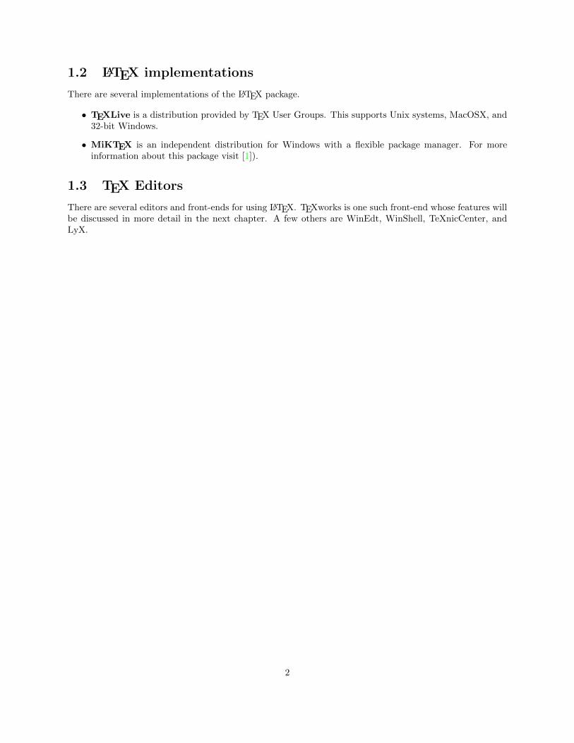
2. A window filling left-half of the screen props up (see Figure 2.2). This is known as the “Editor Wndow”of TEXworks programme.

3. To customise TEXworks, select:

Edit > Preferences ...>

Then the window shown in Fig 2.3 is displayed. In this window four options are available

• General

3

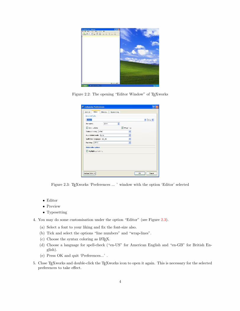
Figure 2.2: The opening “Editor Window” of TEXworks

Figure 2.3: TEXworks ‘Preferences ... ’ window with the option ‘Editor’ selected

• Editor

• Preview

• Typesetting

4. You may do some customisation under the option “Editor” (see Figure 2.3).

(a) Select a font to your liking and fix the font-size also.

(b) Tick and select the options “line numbers” and “wrap-lines”.

(c) Choose the syntax coloring as LATEX.

(d) Choose a language for spell-check (“en-US” for American English and “en-GB” for British En-glish).

(e) Press OK and quit ‘Preferences...’ .

5. Close TEXworks and double-click the TEXworks icon to open it again. This is necessary for the selectedpreferences to take effect.

4

Chapter 3

First Document

3.1 Typesetting a document

There are three stages in typesetting a document using TEX.

1. Create a text file, known as the “input file”, and name it with the extension “.tex”, say for example,sample.tex.

2. The input file is compiled to produce a PDF file. This is the “output file”. The compilation programmeis known as “pdfLATEX”. If the name of the input file is sample.tex the output file would be namedas sample.pdf.

3. View and if necessary print the output file using some PDF reader.

The TEXworks Editor Window is used to create, edit and save the input file. The second and third stagesare executed by applying a single operation, namely, pressing the “typeset” button at the top left corner ofthe TEXworks Editor Window (see Figure 3.1).

If there are no errors in the input file, another window will open up on right half of the monitor and thiswill display the contents of the PDF file generated from the input file. This newly created window is knownas the “Preview Window”.

One cannot print the PDF file from this window. To print it the file has to be opened using some PDFreader.

3.2 First experiment

Let’s now see how to create a first document: for this youll need to type some text in the editor window ofTEXworks. LATEX is not a WYSIWIG (What You See Is What You Get) software, so you’ll have to type thetext and the instructions for formatting it and you’ll see the result only after “typesetting” the text.

Now we are ready to do an experiment. Perform the following operations exactly as instructed.

Figure 3.1: Typeset button in Editor Window in TEXworks

5

Figure 3.2: ‘Save File’ window in TEXworks

3.2.1 Enter text in the Editor Window

Type the following text exactly as shown in the Editor Window of TEXworks programme.

% test01.tex

\documentclass{article}

\title{Test Document}

\author{Student}

\date{}

\begin{document}

\maketitle

My first document typeset with TeX.

\end{document}

3.2.2 Save the text in a file

We now save the text entered in the editor window in a file in the folder MyFolder, which is a folder createdby you. To do this we press the ‘Save’ button. A ‘Save File’ window is opened and we have to navigate toMyFolder. Enter the file name as test01 and press the ‘Save’ bar in the ‘Save File’ window. The contentwill be saved in a file named test01.tex. The TEXworks programme automatically assigns the extension“.tex” to the input file name. The extension .tex is mandatory for all input files.

3.2.3 Typeset and view the document

1. Next we start typesetting the document by clicking the green button in the top left corner of the EditorWindow, or by pressing [Ctrl+T] (see Figure 3.1).

2. A new panel, called Output Panel and labeled Log, opens at the bottom of the Editor Window. Ev-erything LATEX is doing when it works is displayed here. When LATEX finishes (if there is no error) thispanel disappears.

A new window, called the Preview Window, now appears. In this window you can see a page with thefollowing particulars (see Figure 3.3):

• the title “Test Document” centred;

• the name of the author “Student” centred;

• the text “My first document typeset with TeX.”;

6

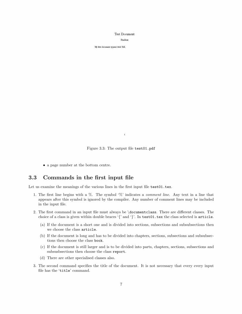
Figure 3.3: The output file test01.pdf

• a page number at the bottom centre.

3.3 Commands in the first input file

Let us examine the meanings of the various lines in the first input file test01.tex.

1. The first line begins with a %. The symbol ‘%’ indicates a comment line. Any text in a line thatappears after this symbol is ignored by the compiler. Any number of comment lines may be includedin the input file.

2. The first command in an input file must always be \documentclass. There are different classes. Thechoice of a class is given within double braces ‘{’ and ‘}’. In test01.tex the class selected is article.

(a) If the document is a short one and is divided into sections, subsections and subsubsections thenwe choose the class article.

(b) If the document is long and has to be divided into chapters, sections, subsections and subsubsec-tions then choose the class book.

(c) If the document is still larger and is to be divided into parts, chapters, sections, subsections andsubsusbsections then choose the class report.

(d) There are other specialised classes also.

3. The second command specifies the title of the document. It is not necessary that every every inputfile has the ‘title’ command.

7

4. The third command specifies the name of the author of the document. The command ‘author’ is alsonot mandatory.

5. The command \date{} is included to suppress the printing of date in the output file. If this commandis not included then the current date will be printed immediately below the name of the author.

6. The content of the document begins with \begin{document} and ends with \end{document}.

7. The text in the input file between \documentclass and \begin{document} is known as the preambleof the document.

8. The command \maketitle gives instructions to the compiler to typeset the title matter of the docu-ment. The title is typeset in a predefined way as specified in the file which describes the specificationsfor the chosen docuumentclass.

3.4 Files generated during compilation

If we examine the folder MyFolder we can see that the folder contains the following files.

1. test01.tex which is the original input file.

2. test01.pdf which is the output file.

3. test01.aux which is an auxiliary file.

4. test01.log which is the log file containing descriptions of what pdfLaTex is doing at the compilationtime.

5. test01.synctex.gz which is a file used for “syncTeX-ing” (see help on TEXworks to know more aboutthis).

Depending on the structure of the document several other associated files are also likely to be created duringcompilation. A few of them are :

• test01.toc : a file created while generating a table of contents.

• test01.lot : a file created while generating a list of tables.

• test01.lof : a file created while generating a list of figures.

• test01.ind, test01.idx, test01.ilg : files created while generating an index.

3.5 When errors occur

When you compile an input file and there is an error, LATEX stops. This is shown by scrolling actions inthe output panel stopping, and an error message is displayed with LATEX waiting for an instruction to knowwhat it should do: one sees the typing cursor in the line between the output panel and the status bar: theconsole bar (see Figure 3.4).

To see the effect, do the following:

1. Go back to the Editor Window by clicking on the window.

2. Change the line \maketitle to \maletitle. The contents are as given below.

8

Figure 3.4: Output panel with error messages

Figure 3.5: Indicator of error in input file

% test02.tex


\title{Test Document}

\author{Student}

\date{}

\begin{document}

\maletitle

My first document typeset with TeX.

\end{document}

3. Save the file as test02.tex.

4. Compile the file by pressing the green button.

5. Wait to see the changes.

The error message reads as follows:

! Undefined control sequence.

l.6 \maketitles

?

The green button will have changed to a red one with a white cross. Click on that button to terminatethe compilation process. The output panel is still visible and so one can still see the error message.

Now correct the errors in the input file, save the file and typeset it by pressing the green button.

9

3.6 Exercises

Before proceeding to the next chapter it is advisable to do some simple exercises. A few changes in the inputfile test01.tex are suggested. You are requested to effect these changes, save the changed file, compile thenew file and preview the output file. Learn the effect of the changes in the input file on the output file.

1. Change the documentclass in test01.tex from article to book.

2. Change the title of the document.

3. Change the name of the author.

4. Delete the command \date{}.

5. Delete the command \maketitle.

6. Write \maketitle after the line ending with typeset with TeX.

10

Chapter 4

Sectioning of Documents

4.1 Sectioning Commands

Any document will naturally be divided into chapters, sections and subsections.

1. To typeset a document with divisions into chapters, sections and subsection, we have to use thefollowing line as the first line of the input file:

\documentclass{book}

2. To start a new chapter with title “New Chapter” include the following line in the input files:

\chapter{New Chapter}

3. To start a new section with title “New Section”, include the following line in the input files:

\section{New Section}

4. To start a new subsection with title “New Subsection”, include the following line in the input files:

\subsection{New Subsection}

5. To start a new subsubsection with title “New Subsubsection”, include the following line in the inputfiles:

\subsubsection{New Subsubsection}

4.2 Example

Enter the following text exactly as shown:

% test03.tex


%

\begin{document}

%

\chapter{First Lessons}

Introductory text.

11

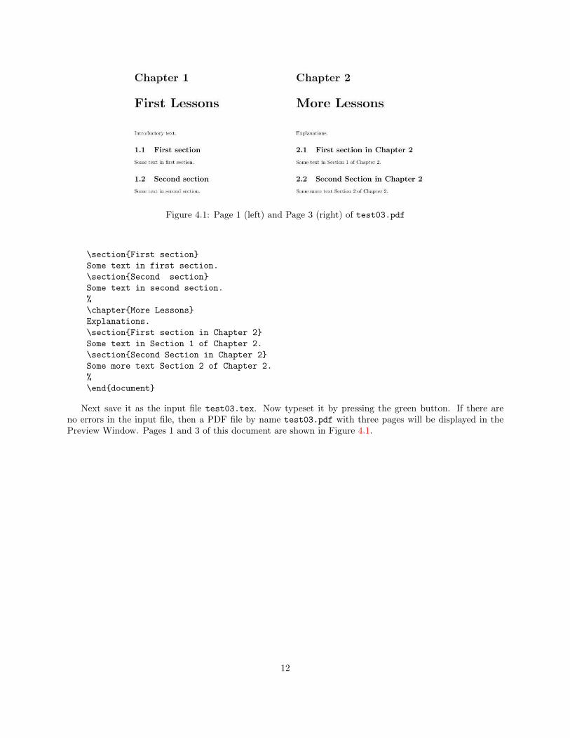
Figure 4.1: Page 1 (left) and Page 3 (right) of test03.pdf

\section{First section}

Some text in first section.

\section{Second section}

Some text in second section.

%

\chapter{More Lessons}

Explanations.

\section{First section in Chapter 2}

Some text in Section 1 of Chapter 2.

\section{Second Section in Chapter 2}

Some more text Section 2 of Chapter 2.

%

\end{document}

Next save it as the input file test03.tex. Now typeset it by pressing the green button. If there areno errors in the input file, then a PDF file by name test03.pdf with three pages will be displayed in thePreview Window. Pages 1 and 3 of this document are shown in Figure 4.1.

12

Chapter 5

Special Characters and Fonts

5.1 Blank Spaces

Blank spaces have no effect except to as word separators. It could be one or many.Blank lines produce new paragraphs. One or many blank lines could be used.

Example

The input file test04.tex produces the output shown in Figure 5.1.

% test04.tex


%

\title{Blank Spaces}

\date{}

\begin{document}

\maketitle

%

Lorem ipsum dolor sit amet,

consectetur adipisicing elit, sed do

eiusmod tempor incididunt ut labore et

dolore magna aliqua. Ut enim ad minim veniam,

quis nostrud exercitation ullamco

laboris nisi ut aliquip ex ea commodo consequat.

Duis aute irure dolor in reprehenderit in

voluptate velit

esse cillum dolore eu fugiat nulla pariatur.

Excepteur sint occaecat cupidatat non

proident, sunt in

culpa qui officia deserunt mollit anim id est laborum.

%

\end{document}

13

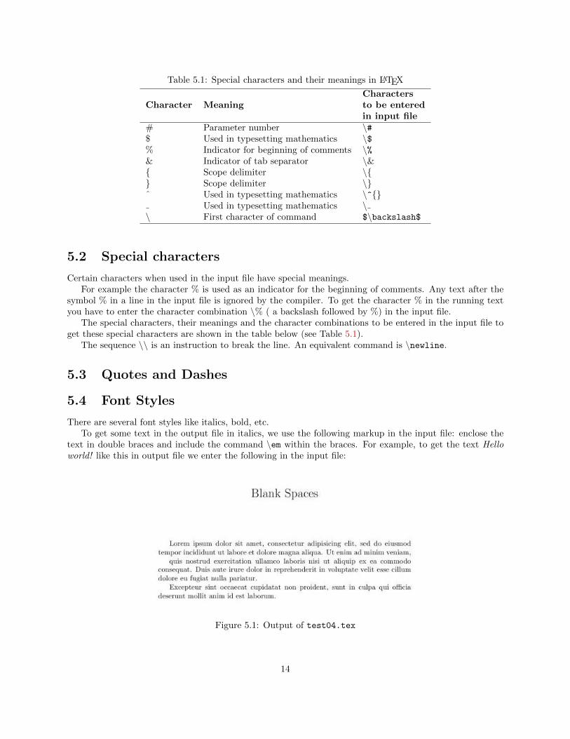
Table 5.1: Special characters and their meanings in LATEX

CharactersCharacter Meaning to be entered

in input file# Parameter number \#$ Used in typesetting mathematics \$% Indicator for beginning of comments \%& Indicator of tab separator \&{ Scope delimiter \{} Scope delimiter \}ˆ Used in typesetting mathematics \^{}

Used in typesetting mathematics \\ First character of command $\backslash$

5.2 Special characters

Certain characters when used in the input file have special meanings.For example the character % is used as an indicator for the beginning of comments. Any text after the

symbol % in a line in the input file is ignored by the compiler. To get the character % in the running textyou have to enter the character combination \% ( a backslash followed by %) in the input file.

The special characters, their meanings and the character combinations to be entered in the input file toget these special characters are shown in the table below (see Table 5.1).

The sequence \\ is an instruction to break the line. An equivalent command is \newline.

5.3 Quotes and Dashes

5.4 Font Styles

There are several font styles like italics, bold, etc.To get some text in the output file in italics, we use the following markup in the input file: enclose the

text in double braces and include the command \em within the braces. For example, to get the text Helloworld! like this in output file we enter the following in the input file:

Figure 5.1: Output of test04.tex

14

Table 5.2: Quotes and dashes

To get EnterQuotesSingle left quote ‘

Single right quote ’

Double left quote ‘‘

Double right quote "

DashesHyphen (inter-word dash) -

Medium dash (number ranges) --

Punctuation dash ---

Table 5.3: Changing font styles

Style Command ExampleTo produce italics style {\em Text} Text

(em for emphasis)To produce bold style {\bf Text} TextTo produce typewriter style {\tt Text} Text

To produce slanted style {\sl Text} TextTo produce small caps style {\sc Text} TextTo produce sans serif style {\sf Text} Text

{\em Hello world!}

The available styles and the markup to produce these styles are tabulated Table 5.3.

5.5 Changing Font Size

There are some standard pre-defined font sizes in LATEX. Running text can be typeset in these font sizes. Forexample, there is a font-size referred to as “huge”. To get the text “Hello world!” in this size the followingmarkup is used.

{\huge Hello world!}

In the output file, the text will appear like this:

Hellow world!Table 5.4 summarises the available commands for changing the font size.

5.6 Changing fonts

We can use different fonts using the following command:

\usefont{code}{family}{series}{shape}

Some of the available fonts with their code, family, series and shapes are given in Table 5.5.For example: to use the Bookman font in bold italics we include the following command:

15

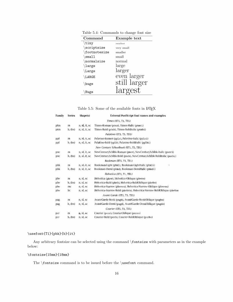
Table 5.4: Commands to change font size

Command Example text\tiny smallest

\scriptsize very small

\footnotesize smaller

\small small

\normalsize normal\large large\Large larger\LARGE even larger\huge still larger\Huge largest

Table 5.5: Some of the available fonts in LATEX

\usefont{T1}{pbk}{b}{it}

Any arbitrary fontsize can be selected using the command \fontsize with parameters as in the examplebelow:

\fontsize{15mm}{18mm}

The \fontsize command is to be issued before the \usefont command.

16

Chapter 6

Some Special Formatting

In this chapter we present a few of the commonly used special formatting of text.

6.1 Centering

Figure 6.1: Example for centered text

The page shown in Figure 6.1 is produced by the following input file.


%

\title{Centred Text}

\date{}

\begin{document}

\maketitle

%





%

17

\begin{center}

quis nostrud exercitation ullamco \\

laboris nisi ut aliquip ex ea commodo \\

consequat. Duis aute irure dolor in

reprehenderit in \\

voluptate velit esse cillum dolore eu

fugiat nulla pariatur.

\end{center}

%


proident, sunt in


%

\end{document}

Observe the following features in this input file.

• the text to be centred is enclosed within an environment which begins with \begin{center} and endswith \end{center}. These behave like the beginning and closing braces.

• Note the spelling of center. It is not centre.

• The two backslashes \\ are used to indicate the end of lines and to instruct the compiler to start anew line.

6.2 One sided justification

6.2.1 Right justification

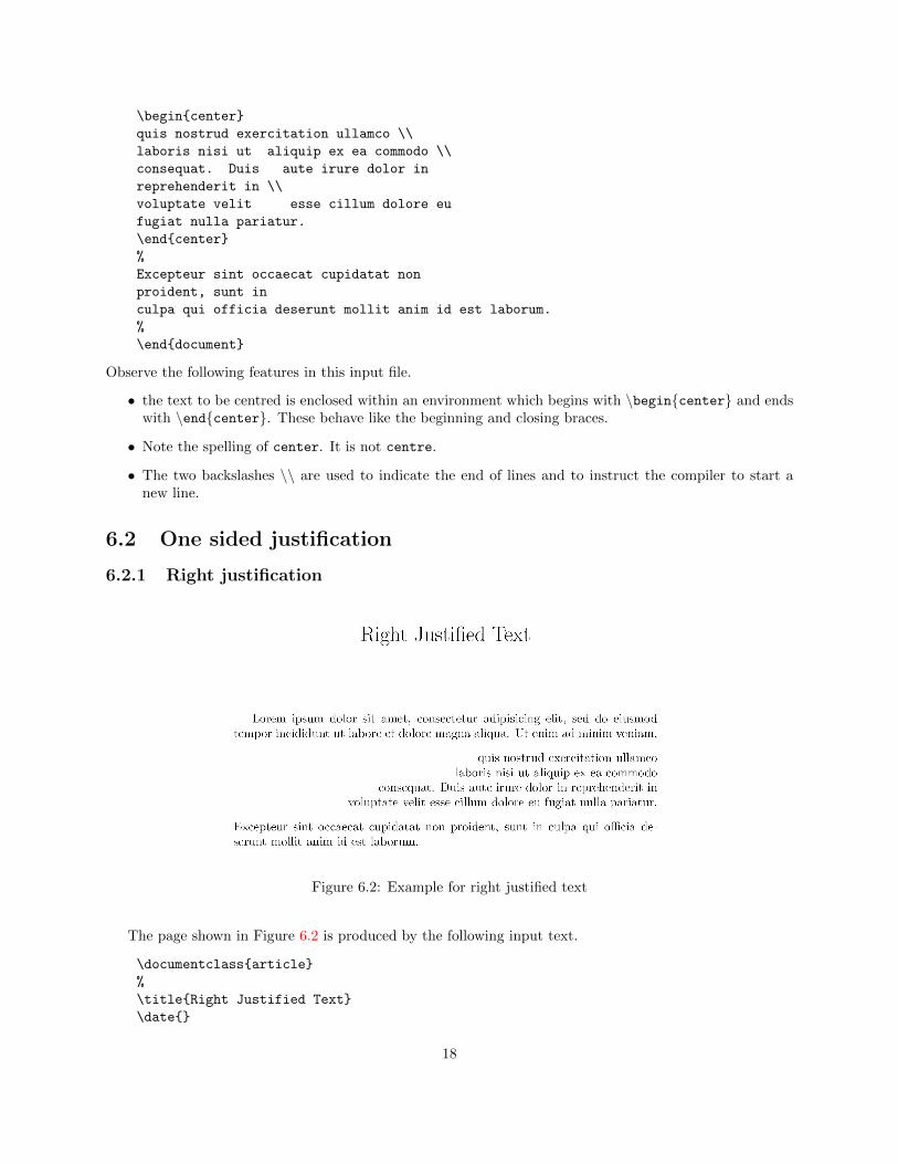
Figure 6.2: Example for right justified text

The page shown in Figure 6.2 is produced by the following input text.


%

\title{Right Justified Text}

\date{}

18

\begin{document}

\maketitle

%





%

\begin{flushright}

quis nostrud exercitation ullamco \\

laboris nisi ut aliquip ex ea commodo \\

consequat. Duis aute irure dolor in

reprehenderit in \\

voluptate velit esse cillum dolore eu fugiat nulla

pariatur.

\end{flushright}

%


proident, sunt in


%

\end{document}


• The text to be right justified is enclosed within an environment which begins with \begin{flushright}and ends with \end{flushright}. These behave like the beginning and closing braces.

• The two backslashes \\ are used to indicate the end of lines and to instruct the compiler to start anew line.

6.2.2 Left justification

Left justified text can be produced in a similar way. For this, one has to replace flushright with flushleft.

6.3 Two-sided justification

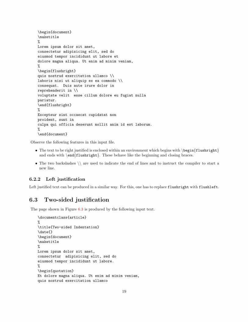
The page shown in Figure 6.3 is produced by the following input text.


%

\title{Two-sided Indentation}

\date{}

\begin{document}

\maketitle

%



eiusmod tempor incididunt ut labore.

%

\begin{quotation}

Et dolore magna aliqua. Ut enim ad minim veniam,

quis nostrud exercitation ullamco

19

Figure 6.3: Example text showing two-sided indentation

laboris nisi ut aliquip ex ea commodo.

Consequat, duis aute irure dolor in

reprehenderit in voluptate velit

esse cillum dolore eu fugiat nulla pariatur.

\end{quotation}

%


proident, sunt in


%

\end{document}


• The text to be right justified is enclosed within an environment which begins with \begin{quotation}and ends with \end{quotation}. These behave like the beginning and closing braces.

6.4 Reproducing typed text

Occasionally it is necessary to print text exactly as it is typed, with all special characters, blanks, and linebreaks appearing literally, unformatted, and in a typewriter font. Lines of computer code or samples ofLATEX input text are examples of such literal text. This is accomplished with the verbatim environment:

\begin{verbatim}text

\end{verbatim}

A new line is inserted before and after these environments.

6.5 Footnotes

Footnotes are generated with the command \footnote{footnote text} which comes immediately after theword requiring an explanation in a footnote.

20

• The text footnote text appears as a footnote in a smaller typeface at the bottom of the page.

• The first line of the footnote is indented and is given the same footnote marker as that inserted in themain text.

• The first footnote on a page is separated from the rest of the page text by means of a short horizontalline.

• Footnotes are numbered serially in the article class.

• Footnote numbering is reset to 1 for each new chapter for book and report classes.

21

Chapter 7

Lists

7.1 Itemization

7.1.1 Simple Itemized List

Let it be required to produce the following list in the outputfile:

• Civil Engg

• Computer Science

• Mechanical Engg

• Production Engg

• EEE

• E& C Engg

We enter the following in the input file.

\begin{itemize}

\item Civil Engg

\item Computer Science

\item Mechanical Engg

\item Production Engg

\item EEE

\item E\& C Engg

\end{itemize}

7.1.2 Nested Itemized List

Let it be required to produce the following in the outputfile.

• Civil Engg

– Teaching Staff

∗ Professor

∗ Lecturers

– Non-teaching Staff

22

• Computer Science

– Teaching Staff


• Mechanical Engg

– Teaching Staff


• Production Engg

– Teaching Staff


• EEE

• E& C Engg

We enter the following in the input file.

\begin{itemize}

\item Civil Engg

\begin{itemize}

\item Teaching Staff

\begin{itemize}

\item Professor

\item Lecturers

\end{itemize}

\item Non-teaching Staff

\end{itemize}


\begin{itemize}



\end{itemize}


\begin{itemize}



\end{itemize}


\begin{itemize}



\end{itemize}

\item EEE

\item E\& C Engg

\end{itemize}

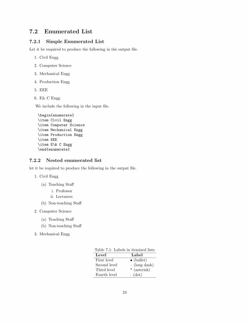
In itemized (bulleted) lists labels are assigned as per the scheme in Table 7.1.

23

7.2 Enumerated List

7.2.1 Simple Enumerated List

Let it be required to produce the following in the output file.

1. Civil Engg

2. Computer Science

3. Mechanical Engg

4. Production Engg

5. EEE

6. E& C Engg

We include the following in the input file.

\begin{enumerate}

\item Civil Engg




\item EEE

\item E\& C Engg

\end{enumerate}

7.2.2 Nested enumerated list

let it be required to produce the following in the output file.

1. Civil Engg

(a) Teaching Staff

i. Professor

ii. Lecturers

(b) Non-teaching Staff

2. Computer Science

(a) Teaching Staff


3. Mechanical Engg

Table 7.1: Labels in itemized lists

Level LabelFirst level • (bullet)Second level – (long dash)Third level * (asterisk)Fourth level . (dot)

24

Table 7.2: Labels in enumerated lists

Level Labels DescriptionFirst level 1. ,2. , Arabic numerals with a periodSecond level (a), (b), Lower case letters in parenthesesThird level i. ii. , Lower case Roman numerals with a periodFourth level A , B , Capital letters

(a) Teaching Staff


4. Production Engg

(a) Teaching Staff


5. EEE

6. E& C Engg

We include the following in the input file:

\begin{enumerate}

\item Civil Engg

\begin{enumerate}


\begin{enumerate}

\item Professor

\item Lecturers

\end{enumerate}


\end{enumerate}


\begin{enumerate}



\end{enumerate}


\begin{enumerate}



\end{enumerate}


\begin{enumerate}



\end{enumerate}

\item EEE

\item E\& C Engg

\end{enumerate}

In enumerated lists, the labels are assigned as specified in Table 7.2.

25

Chapter 8

Tables

8.1 Simple Tables

8.1.1 Tables with horizontal and vertical lines

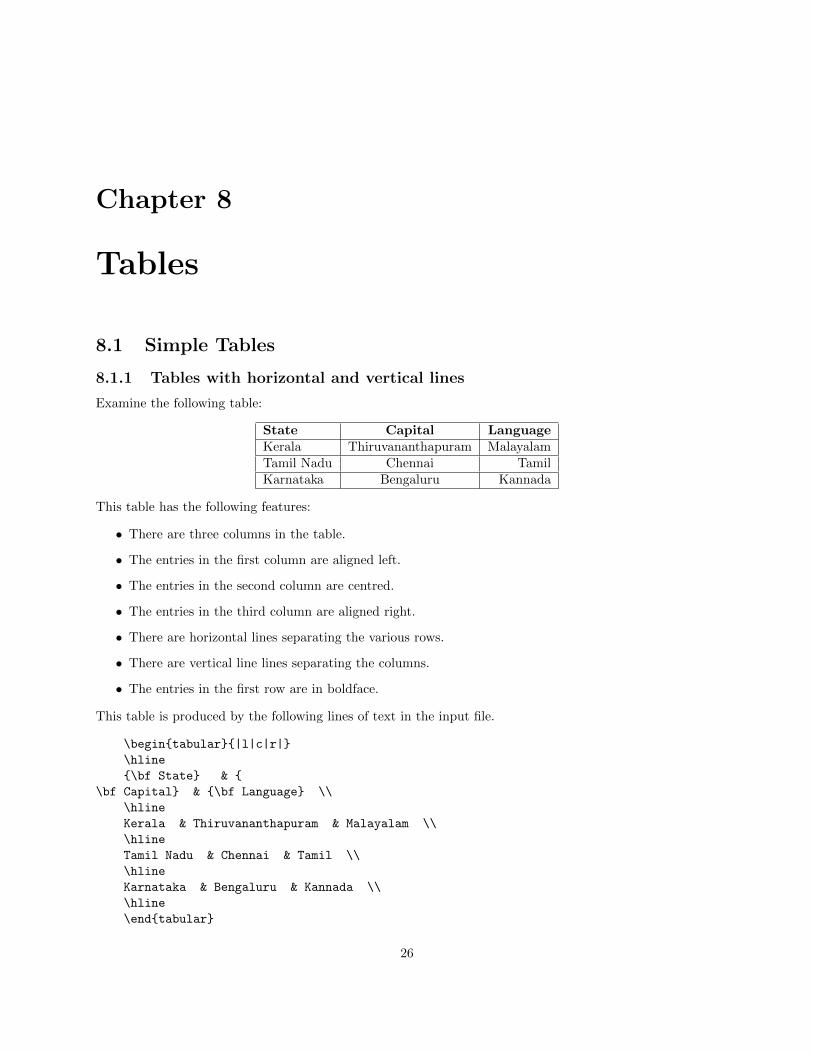
Examine the following table:

State Capital LanguageKerala Thiruvananthapuram MalayalamTamil Nadu Chennai TamilKarnataka Bengaluru Kannada

This table has the following features:

• There are three columns in the table.

• The entries in the first column are aligned left.

• The entries in the second column are centred.

• The entries in the third column are aligned right.

• There are horizontal lines separating the various rows.

• There are vertical line lines separating the columns.

• The entries in the first row are in boldface.

This table is produced by the following lines of text in the input file.

\begin{tabular}{|l|c|r|}

\hline

{\bf State} & {

\bf Capital} & {\bf Language} \\

\hline

Kerala & Thiruvananthapuram & Malayalam \\

\hline

Tamil Nadu & Chennai & Tamil \\

\hline

Karnataka & Bengaluru & Kannada \\

\hline

\end{tabular}

26

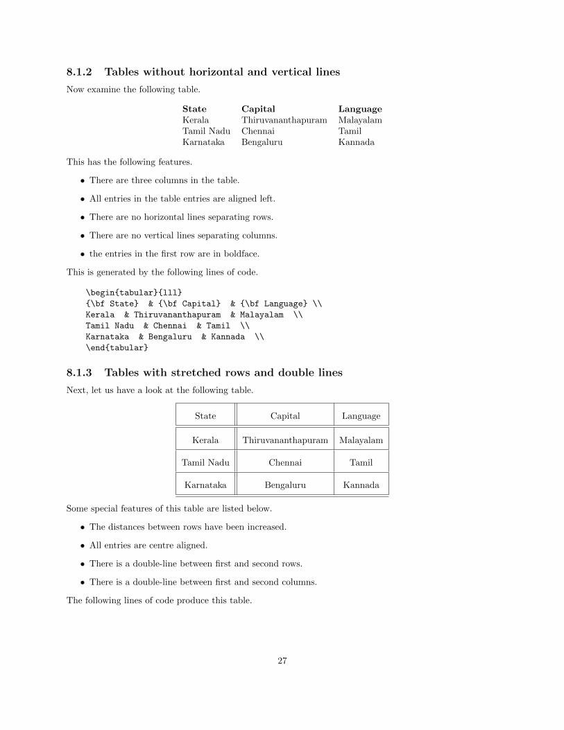
8.1.2 Tables without horizontal and vertical lines

Now examine the following table.

State Capital LanguageKerala Thiruvananthapuram MalayalamTamil Nadu Chennai TamilKarnataka Bengaluru Kannada

This has the following features.

• There are three columns in the table.

• All entries in the table entries are aligned left.

• There are no horizontal lines separating rows.

• There are no vertical lines separating columns.

• the entries in the first row are in boldface.

This is generated by the following lines of code.

\begin{tabular}{lll}

{\bf State} & {\bf Capital} & {\bf Language} \\




\end{tabular}

8.1.3 Tables with stretched rows and double lines

Next, let us have a look at the following table.

State Capital Language

Kerala Thiruvananthapuram Malayalam

Tamil Nadu Chennai Tamil

Karnataka Bengaluru Kannada

Some special features of this table are listed below.

• The distances between rows have been increased.

• All entries are centre aligned.

• There is a double-line between first and second rows.

• There is a double-line between first and second columns.

The following lines of code produce this table.

27

\renewcommand{\arraystretch}{2}

\begin{tabular}{|c||c|c|c|}

\hline

State & Capital & Language \\

\hline\hline


\hline


\hline


\hline

\hline

\end{tabular}

Here \arraystretch is the command to increase the distance between rows. The number ‘2’ is the value ofthe parameter which specifies how much the distances between rows have to be increased. If we require stillhigher distances replace this by a higher value. The value ‘1’ gives the normal distance.

Tables with cells in paragraph mode Study the next table.


Kerala Thiruvananthapuram The language of the stateis Malayalam.

Tamil Nadu Chennai The language is Tamil, aclassical language.

Karnataka Bengaluru Kannada is the languageof the state.

Sometimes the entries to be written into a cell may be longer. Usually there will be only one line in a cell.However, we can have cells with multiple lines of text by typesetting cells in the ‘paragraph mode’. theabove table is an example for such a table. It is produced by the following lines of code.

\renewcommand{\arraystretch}{2}

\begin{tabular}{|c||l|p{4cm}|}

\hline


\hline\hline

Kerala & Thiruvananthapuram

& The language of the state is Malayalam. \\

\hline

Tamil Nadu & Chennai

& The language is Tamil, a classical language. \\

\hline

Karnataka & Bengaluru

& Kannada is the language of the state. \\

\hline \hline

\end{tabular}

The code p{4cm} specifies that the third column is to be typeset in the paragraph mode, the horizontalwidth of the cells in the column being 4 cm.

28

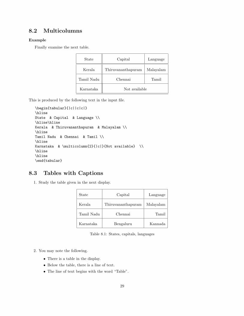
8.2 Multicolumns

Example

Finally examine the next table.




Karnataka Not available

This is produced by the following text in the input file.

\begin{tabular}{|c||c|c|}

\hline


\hline\hline


\hline


\hline

Karnataka & \multicolumn{2}{|c|}{Not available} \\

\hline

\hline

\end{tabular}

8.3 Tables with Captions

1. Study the table given in the next display.




Karnataka Bengaluru Kannada

Table 8.1: States, capitals, languages

2. You may note the following.

• There is a table in the display.

• Below the table, there is a line of text.

• The line of text begins with the word “Table”.

29

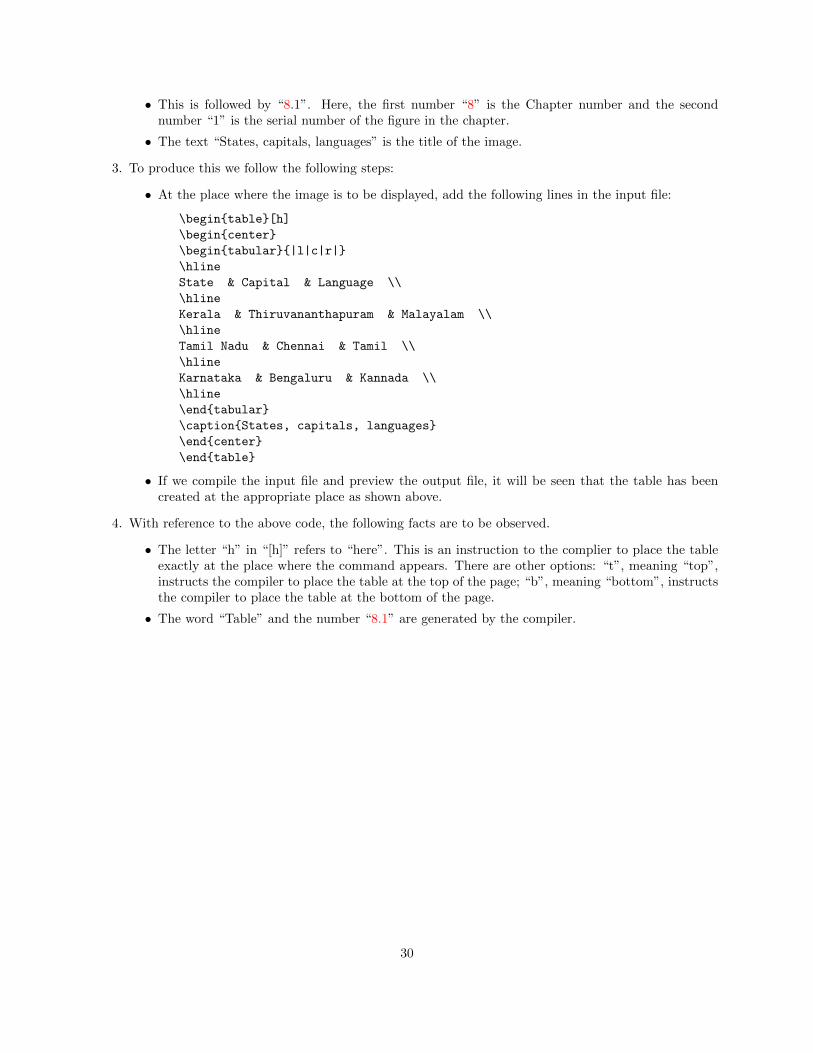
• This is followed by “8.1”. Here, the first number “8” is the Chapter number and the secondnumber “1” is the serial number of the figure in the chapter.

• The text “States, capitals, languages” is the title of the image.

3. To produce this we follow the following steps:

• At the place where the image is to be displayed, add the following lines in the input file:

\begin{table}[h]

\begin{center}

\begin{tabular}{|l|c|r|}

\hline


\hline


\hline


\hline


\hline

\end{tabular}

\caption{States, capitals, languages}

\end{center}

\end{table}

• If we compile the input file and preview the output file, it will be seen that the table has beencreated at the appropriate place as shown above.

4. With reference to the above code, the following facts are to be observed.

• The letter “h” in “[h]” refers to “here”. This is an instruction to the complier to place the tableexactly at the place where the command appears. There are other options: “t”, meaning “top”,instructs the compiler to place the table at the top of the page; “b”, meaning “bottom”, instructsthe compiler to place the table at the bottom of the page.

• The word “Table” and the number “8.1” are generated by the compiler.

30

Chapter 9

Graphics

9.1 A picture in a document

Study the following display:

Figure 9.1: TeX Lion

You may note the following.

• There is an image1 in the display.

• Below the image there is a line of text.

• The line of text begins with the word “Figure”.

• This is followed by “9.1”. Here, the first number “8” is the Chapter number and the second number“1” is the serial number of the figure in the chapter.

• The text “TeX Lion” is the title of the image.

9.2 Putting a picture in input file

To produce a picture in a file we follow the following steps:

• Save the image as a .JPG file, say texlion.JPG, in MyFolder.

1CTAN (Comprehensive TeX Archive Network) lion drawing by Duane Bibby; thanks to www.ctan.org.

31

Figure 9.2: TeX Lion enlarged

Figure 9.3: TeX lion compressed

• Add the command \usepackage{graphicx} in the preamble of the document. (Note the spelling ofthe package; it ends with an ”x”.)

• At the place where the image is to be displayed, add the following lines in the input file:

\begin{figure}[h]

\begin{center}

\includegraphics{texlion.JPG}

\caption{TeX Lion}

\end{center}

\end{figure}

• If we compile the input file and preview the output file, it will be seen that the image has been createdat the appropriate place as shown above.

• With reference to the above code, the following facts are to be observed.

– The letter “h” in “[h]” refers to “here”. This is an instruction to the complier to place the imageexactly at the place where the command appears. There are other options: “t”, meaning “top”,instructs the compiler to place the figure at the top of the page; “b”, meaning “bottom”, instructsthe compiler to place the figure at the bottom of the page.

– The word “Figure” and the number “9.1” are generated by the compiler.

• Several options are available to control the size of the image.

– If the image is to be displayed with a width of 7 cm, the command is to be modifies as follows.

32

\includegraphics[width = 7cm]{texlion.JPG}

With this changed command the output figure will be as in Figure 9.2.

– We can also specify the height. If the height of the displayed image in the output file is to be 2cm, it is specified as follows:

\includegraphics[height = 2cm]{texlion.JPG}

The output image will now appear as in Figure 9.3.

33

Chapter 10

Mathematics

TEX was created to typeset documents containing a lot of mathematics. So TEX and LATEX have a largenumber of features to produce beautifully typeset mathematics. This chapter is only a first introduction tothis vast area of LATEX. More elaborate descriptions can be found in the literature. For example see [?] or[4].

10.1 amsmath package

When typesetting mathematics always load the amsmath package. This package contains several featuresdeveloped by the American Mathematical Society (AMS). (For a detailed discussion see [5].)

\usepackage{amsmath}

10.2 First lessons

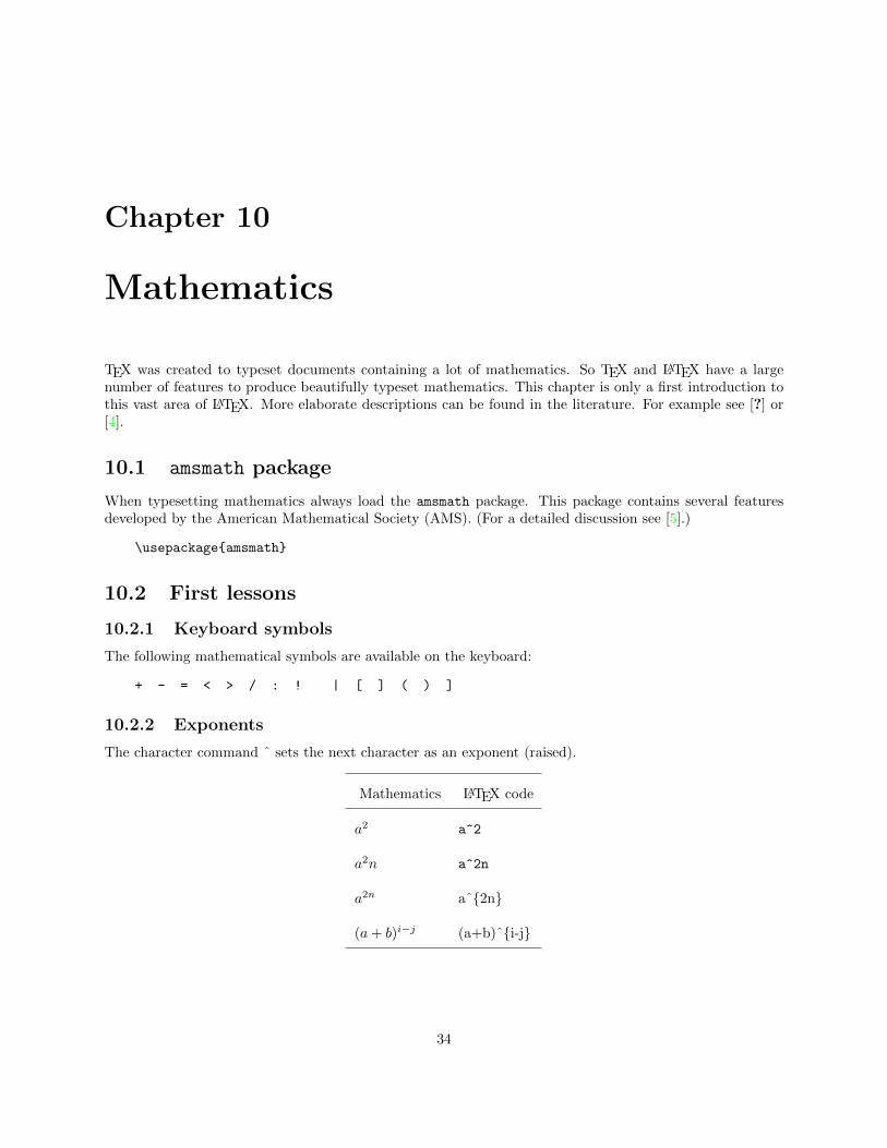
10.2.1 Keyboard symbols

The following mathematical symbols are available on the keyboard:

+ - = < > / : ! | [ ] ( ) ]

10.2.2 Exponents

The character command ˆ sets the next character as an exponent (raised).

Mathematics LATEX code

a2 a^2

a2n a^2n

a2n aˆ{2n}

(a+ b)i−j (a+b)ˆ{i-j}

34

10.2.3 Subscripts

The character command sets the next character as an index (lowered).


a2 a 2

a2n a 2n

a2n a {2n}

(a+ b)i−j (a+b) {i-j}

10.2.4 Both exponents and indices

Multiple raisings and lowerings are generated by applying ˆ and to the exponents and indices


xy2

x^{y^2}

xy1 x^{y 1}

Ax2i

j2nn,mA^{x i^2} {j^{2n} {n,m} }

10.2.5 Fractions


ab \frac{a}{b}

a2−b2

a−b \frac{a^2 - b^2}{a-b}ab

1+ cd

\frac{\frac{a}{b}} {1 + \frac{c}{d}}

10.2.6 Roots


√A+B \sqrt{A+B}

3√A+B \sqrt[3]{A+B}

3

√−q +

√q2 + p3 \sqrt[3]{- q + \sqrt{q^2 + q^3 }}

35

10.2.7 Mathematical symbols

There is a very wide range of symbols used in mathematical text. Only a few are directly available from thekeyboard. LATEX provides many of the mathematical symbols that are commonly used. They are called withthe symbol name prefixed with the \ character. The names themselves are derived from their mathematicalmeanings. For example to get π we type \pi and to get ± type \pm. Hundreds of such symbols can be usedin LATEX. A comprehensive list of all mathematical and other symbols that can be used in LATEX is availableat [6].

10.3 Mathematics in input file

10.3.1 Mathematical expressions inline

To produce equations and formulas inline use one the following formats:

\begin{math} formula text \end{math}

$ formula text $

$ formula text $

Example input:

The equation $ax+b=0$ has no solution when $a=0$ and $b\ne 0$.

Example output:

The equation ax+ b = 0 has no solution when a = 0 and b 6= 0.

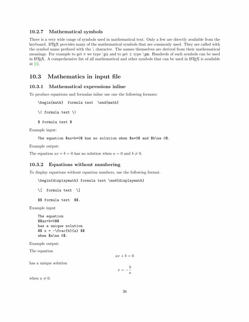
10.3.2 Equations without numbering

To display equations without equation numbers, use the following format.

\begin{displaymath} formula text \end{displaymath}

\[ formula text \]

$$ formula text $$.

Example input

The equation

$$ax+b=0$$

has a unique solution

$$ x = -\frac{b}{a} $$

when $a\ne 0$.

Example output:

The equationax+ b = 0


x = − ba

when a 6= 0.

36

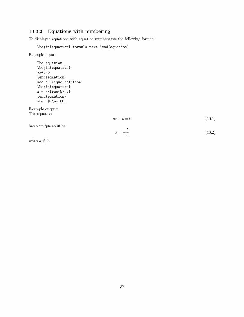
10.3.3 Equations with numbering

To displayed equations with equation numbers use the following format:

\begin{equation} formula text \end{equation}

Example input:

The equation

\begin{equation}

ax+b=0

\end{equation}


\begin{equation}

x = -\frac{b}{a}

\end{equation}

when $a\ne 0$.

Example output:The equation

ax+ b = 0 (10.1)


x = − ba

(10.2)

when a 6= 0.

37

Chapter 11

Cross References

11.1 Outline of procedure

Let there be several figures and tables in a document. Let it be required to refer to these figures and tablesat other points in the document. Cross referencing methods are used to tackle this problem.

Cross referencing involves three steps:

1. Assigning labels to items to be referenced. Some of the items to which labels can be assigned are thefollowing:

• Tables

• Figures

• Chapter numbers

• Section numbers

• Equation numbers

• Page numbers

• Items in enumerated lists.

Items are assigned labels using the ‘\label’ command.

2. Inserting commands in the input files indicating the places where these references are to be printed.These are inserted using the ‘\ref’ and ‘\pageref’ commands.

3. Compiling the input file to get the the references properly printed in the output file. To get thereferences printed, the input file is to compiled twice.

• In the first compilation the programme collects all the labels and stores them in a file.

• During the second compilation the labels are assigned values and placed at the appropriate loca-tions.

11.2 Assigning labels

11.2.1 Assigning labels to tables and figures

We have seen in Section 8.3 how to produce captions to tables. To reference a table at another point in thedocument, we assign a unique label to the table. The label may be any combination of letters, numbers, orsymbols. Let the label be MyLabel. The command to assign this label is

38

\label{MyLabel}.

Include this command immediately after the closing brace of the \caption command. The compiler assignsto the label MyLabel a value which is the number assigned to the table by the compiler.

The procedure described above can also be applied to assign a unique label to every figure in a document.Examples:

\caption{States, capitals, languages}\label{FirstTable}

\caption{An image of TeXlion}\label{Fig:001}

11.2.2 Assigning labels to chapters, sections, etc.

Labels can be assigned to chapter numbers, section numbers, etc. using the \label command. We writethis command adjacent to the respective sectioning commands as in the following examples.

\chapter{Introduction}\label{xyz}

\section{Prliminaries}\label{ch1.sec.001}

\subsection{Basics}\label{ab:123}

11.2.3 Assigning labels to equations

The number assigned to an equation with numbering can be assigned to a label by invoking the \labelcommand. The next example illustrates the procedure.

\begin{equaion}\label{Eq.1}

(a+b)^2=a^2+2ab+b^2

\end{equation}

11.2.4 Assigning labels to page numbers

A page number can be assigned a label by issuing the \label command in the page.

11.3 Printing the value of a label

The value assigned to a label is printed by using the \ref command. If the label is Mylabel, the value ofthis label is printed by issuing the command \ref{Mylabel}.

The page number on which the \label command was issued can be printed with

\pageref{marker}

at any point earlier or later in the document.

11.4 Example for cross referencing

11.4.1 Example input file


\usepackage{graphicx}

\begin{document}

\chapter{Cross Referencing}

Some examples.

\section{Tables and figures}

%

Consider the following table:

39

Figure 11.1: Example for cross referencing

\begin{table}[h]

\begin{center}

\begin{tabular}{ll}

\hline

State & Capital \\

\hline

Kerala & Thiruvanathapuram \\

Tamiil Nadu & Chennai \\

\hline

\end{tabular}

\end{center}

\caption{States and capitals}\label{Table:01}

\end{table}

Next consider the following figure:

\begin{figure}[h]

40

\begin{center}

\includegraphics[height = 2cm]{texlion.JPG}

\end{center}

\caption{TeX lion}\label{Figure:01}

\end{figure}

\section{References to tables and figures}

The picture in Figure \ref{Figure:01} is a

compressed image of the TeXLion. The data in Table

\ref{Table:01} is a short table of states and their

capitals.

\end{document}

11.4.2 Example output file

The output of the input file given in Section 11.4.1 is shown in Figure 11.1.

41

Chapter 12

Simple Index

12.1 Procedure

The various steps for the creation of an index are summarised below.

1. If an index is to be created, the package makeidx must be loaded. This is done by including thefollowing line in the preamble:

\usepackage{makeidx}

2. Next the command \makeindex must also be included in the preamble. (Note that the package ismakeidx and the command is makeindex.)

3. Include the command \printindex at the end of the document.

4. In the main body of the document, mark those entries which are to be included in the index as follows:Let the entry to be included in index be “Automation”. The we mark it as

\index{Automation}

In this way mark all other entries also.

5. We compile the source file by running pdfLATEX once.

6. Next we have to run an external program known as MakeIndex.

7. Next we have to compile the document again by running pdfLATEX once more.

8. The output file now would have a properly placed index.

12.2 Example

Input file


\usepackage{makeidx}

\makeindex

%

\begin{document}

%

42

\chapter{First}

\section{Examples}

We have included example words like

Zizigy\index{Zizigy} and Automation\index{Automation}

in this section.

\section{More exapmles}

A few more examples are included here like

computer\index{computer}, \index{compiler}

which are common words. Ordinary words can

also be included in index.

%

\printindex

\end{document}

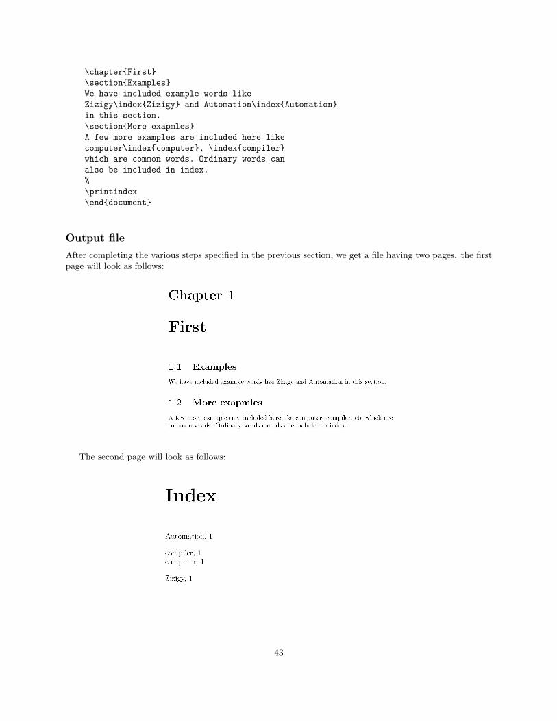
Output file

After completing the various steps specified in the previous section, we get a file having two pages. the firstpage will look as follows:

The second page will look as follows:

43

Chapter 13

Generating Bibliography

13.1 Sample bibliography

Let it be required to produce a bibliography as follows.

13.2 LATEX code for the sample bibliography

This produced by including the following text at the end of the document.

\begin{thebibliography}{99}

%

\bibitem{xyz}

A Kanetkar, {\em Let Us C}, Prentice hall of India, 2009.

\bibitem{abc}

D E Knuth, {\em The TeXbook}, Academic Press, 1990.

\bibitem{LabelX}

Sommerville, {\em Textbook of Software Engineering},

Pearson education, 2010.

%

\end{thebibliography}

44

13.3 Explanatory notes

The following facts may be observed.

1. The content of the bibliography is placed inside the environment

\begin{thebibliography}{sample label}

entries

\end{thebibliography}

2. Each of the individual entries in the bibliography begins with the command

\bibitem{key}

entry text

The keyword \bibitem produces a running number in square brackets as the label for the reference inthe text.

The mandatory argument key is a reference key, which is like the cross-referencing key \label usedto make the actual citation in the main text. The key name can be made up of any combination ofletters, numbers, and symbols except commas.

3. The citation in the text is made with the command

\cite{key}

where key is the reference key that appears in the \bibitem command.

13.4 The bibtex package

BibTEX is a tool specially devised to handle long lists of references. This tool allows us to store all ourreferences in an external database. We can then easily link this database to any LATEX document, and citeany reference that is contained within the file. This is often more convenient than embedding them at theend of every document we write. We can have a centralised store of our bibliography, that can be linked toas many documents as we wish. For more details see ??.

45

Chapter 14

Page Layouts

14.1 Page layout parameters

Page layout is concerned with the design of a page. The dimensions of the margins (left, right, top andbottom), page orientation (portrait or landscape) and number of columns in a page are some of the elementsthat go into the design of a page.

Figure 14.1 (page 47) shows some of the important page layout parameters and the LATEX commands tospecify these parameters.

14.2 geometry package

The geometry package can be used to specify the values of the page layout parameters. With this package,one can easily give values for some of the layout parameters, and the rest will be set automatically, takinginto account. For example, to set \textwidth to 15 cm and \textheight to 25 cm on A4 paper, one gives

\usepackage{geometry}

\geometry{a4paper,textwidth=15cm,textheight=25cm}

which will also automatically set \oddsidemargin and \topmargin so that the text is centered horizontallyand vertically, including the head and footlines. Or, one can set all the margins to be 1 inch on US letterpaper with

\geometry{letterpaper,margin=1in}

\end{vebatim}

%

Rather than using the {\tt \textbackslash{}geometry} command, one may also place the

parameters as options to {\tt \textbackslash{}usepackage}, for example as

%

\begin{verbatim}

\usepackage[a4paper,left=3cm,right=2cm]{geometry}

to set the left and right margins to definite values, and \textwidth to what is left over. In general, allthe parameters in Figure 14.1 may be specified by geometry by giving their names (without the backslashcharacter).

For more details on geometry package refer to manual written by the creator of the package (see [8]).

46

Figure 14.1: Page Layout Parameters

47

Chapter 15

Book Structure

15.1 Front matter, main matter, back matter

The contents of a book can be classified as belonging to three different types of structures.

• Front matter: This consists of preface, acknowledgment, dedication, table of contents, list of tables,list of figures, etc.

• Main matter: This is the main body of the book.

• Back matter: This contains bibliography, index, colophon, etc.

In well-structured books the three parts are typeset differently. Commands have been provided in the book

class to typeset these three elements of a book as per well established conventions.

• The \frontmatter command switches page numbering to Roman numerals and suppresses the num-bering of chapters. This command is issued immediately prior to the point where the front matter ofthe book begins.

• The \mainmatter command resets the page numbering to 1 with Arabic numbers and reactivates thechapter numbering. This command is issued immediately prior to the point where the main matter ofthe book begins.

• Finally the \backmatter command is issued immediately prior to the point where the back mattersof the book begin.

15.2 Front matter

15.2.1 Table of contents

The table of contents is generated and printed with the command

\tableofcontents

given at the location where the table of contents is to appear, which is normally after the title page andabstract.

To generate a table of contents, the input file has to be compiled at least twice.

48

15.2.2 Other lists

In addition to the table of contents, lists of figures and tables can also be generated and printed automaticallyby LATEX. The commands to produce these lists are

\listoffigures

\listoftables

The entries in these lists are made automatically by the \caption command in the figure and table environ-ments.

15.3 Splitting of documents

When an input file is large, it would be better to split the work into several smaller files. LATEX then mergesthese smaller files during the processing.

The contents of another file may be read into a LATEX document with the command

\input{filename}

where the name of the other file is filename.tex. It is only necessary to specify the full name of the file if theextension is something other than .tex. During the LATEX processing, the text contained in this second fileis read in at that location in the first file where the command is given. The result of the \input command isthe same as if the contents of the file filename.tex had been typed into the document file at that position.The command may be given anywhere in the document, either in the preamble or within the text part.

49

Appendix : The Name of the Game

The following is a verbatim reproduction of “Chapter 1 The Name of the Game” in [11] which is the manualof the TEX program written by the creator of the program.

English words like ‘technology’ stem from a Greek root beginning with the letters τ , ε, χ,. . .; and thissame Greek word means art as well as technology. Hence the name TEX, which is an uppercase form of τεχ.

Insiders pronounce the χ of TEX as a Greek chi, not as an ‘x’, so that TEX rhymes with the word blecchhh.It’s the ’ch’ sound in Scottish words like loch or German words like ach; it’s a Spanish ’j’ and a Russian ’kh’.When you say it correctly to your computer, the terminal may become slightly moist.

The purpose of this pronunciation exercise is to remind you that TEX is primarily concerned with high-quality technical manuscripts: Its emphasis is on art and technology, as in the underlying Greek word. If youmerely want to produce a passably good document – something acceptable and basically readable but notreally beautiful – a simpler system will usually suffice. With TEX the goal is to produce the finest quality;this requires more attention to detail, but you will not find it much harder to go the extra distance, andyou’ll be able to take special pride in the finished product. On the other hand, it’s important to noticeanother thing about TEX’s name: The ’E’ is out of kilter. This displaced ’E’ is a reminder that TEX isabout typesetting, and it distinguishes TEX from other system names. In fact, TEX (pronounced tecks)is the admirable Text EXecutive processor developed by Honeywell Information Systems. Since these twosystem names are pronounced quite differently, they should also be spelled differently. The correct way torefer to TEX in a computer file, or when using some other medium that doesn’t allow lowering of the ’E’, isto type ’TeX’. Then there will be no confusion with similar names, and people will be primed to pronounceeverything properly.

EXERCISE 1.1After you have mastered the material in this book, what will you be: A TEXpert, or a TEXnician?

They do certainly givevery strange and new-fangled names to diseases.– PLATO, The Republic, Book 3 (c. 375 B.C.)

Technique! The very word is like the shriekOf outraged Art. It is the idiot name

Given to effort by those who are too weak,Too weary, or too dull to play the game.

– LEONARD BACON, Sophia Trenton (1920)

50

Bibliography

[1] MiKTEX project page: Available: http://miktex.org/

[2] Instructions for downloading and installing MikTEX 2.8: Available: http://miktex.org/2.8/setup

[3] Comparison of TEX editors (IDEs), Wikipedia, The Free Encyclopedia: Available: http://en.

wikipedia.org/wiki/Comparison_of_TeX_editors

[4] Chapter 8 of “The LaTeX Companion” by Frank Mittelbach and Michel Goosens. Available: http:

//www.macrotex.net/texbooks/latexcomp-ch8.pdf.

[5] Users Guide for the amsmath Package. Available: ftp://ftp.ams.org/pub/tex/doc/amsmath/

amsldoc.pdf.

[6] The comprehensive LaTeX symbols list. Available: http://www.ctan.org/tex-archive/info/

symbols/comprehensive/symbols-a4.pdf.

[7] MakeIndex: An Index Processor For LaTEX, Leslie Lamport. Available: http://www.tex.ac.uk/

tex-archive/indexing/makeindex/doc/makeindex.pdf, 1987.

[8] The geometry package, Hideo Umeki. Available: ftp://ftp.tex.ac.uk/tex-archive/macros/latex/contrib/geometry/geometry.pdf

[9] Tame the BeaST : The B to X of BibTEX, Nicolas Markey, 2009. Available: http://www.ctan.org/

tex-archive/info/bibtex/tamethebeast/ttb_en.pdf

[10] LATEX , Wikibooks contributors. Available: http://upload.wikimedia.org/wikipedia/commons/2/

2d/LaTeX.pdf

[11] The TEXbook, Donald E Knuth, Addison-Wesley Publishing Company, 1991. Available: http://net.

ytu.edu.cn/share/%D7%CA%C1%CF/texbook.pdf

51

http://miktex.org/

http://miktex.org/2.8/setup

http://en.wikipedia.org/wiki/Comparison_of_TeX_editors

http://en.wikipedia.org/wiki/Comparison_of_TeX_editors

http://www.macrotex.net/texbooks/latexcomp-ch8.pdf

http://www.macrotex.net/texbooks/latexcomp-ch8.pdf

ftp://ftp.ams.org/pub/tex/doc/amsmath/amsldoc.pdf

ftp://ftp.ams.org/pub/tex/doc/amsmath/amsldoc.pdf

http://www.ctan.org/tex-archive/info/symbols/comprehensive/symbols-a4.pdf

http://www.ctan.org/tex-archive/info/symbols/comprehensive/symbols-a4.pdf

http://www.tex.ac.uk/tex-archive/indexing/makeindex/doc/makeindex.pdf

http://www.tex.ac.uk/tex-archive/indexing/makeindex/doc/makeindex.pdf

ftp://ftp.tex.ac.uk/tex-archive/macros/latex/contrib/geometry/geometry.pdf

ftp://ftp.tex.ac.uk/tex-archive/macros/latex/contrib/geometry/geometry.pdf

http://www.ctan.org/tex-archive/info/bibtex/tamethebeast/ttb_en.pdf

http://www.ctan.org/tex-archive/info/bibtex/tamethebeast/ttb_en.pdf

http://upload.wikimedia.org/wikipedia/commons/2/2d/LaTeX.pdf


http://net.ytu.edu.cn/share/%D7%CA%C1%CF/texbook.pdf

http://net.ytu.edu.cn/share/%D7%CA%C1%CF/texbook.pdf

References

1. Online resource

(a) LATEX , Wikibooks contributors. Available: http://upload.wikimedia.org/wikipedia/commons/2/2d/LaTeX.pdf

(b) The Not So Short Introduction to LATEX2, Or LATEX2e in 157 minutes, Tobias Oetiker HubertPartl, Irene Hyna and Elisabeth Schlegl. Available: http://www.ctan.org/tex-archive/info/lshort/english/lshort.pdf

(c) Online tutorials on LATEX, Indian TEX Users’ Group. Available: http://tug.org.in/tutorials.html

(d) TEX Resources on the Web. Available: http://www.tug.org/interest.html#latexbooks

2. Standard reference books

(a) A Guide to LATEX2e, by Helmut Kopka and Patrick Daly (Addison-Wesley, ISBN 0-321-17385-6,fourth edition, 2003).

(b) The LATEX Companion, by Frank Mittelbach, Michel Goossens, Johannes Braams, David Carlisle,and Chris Rowley (Addison-Wesley, ISBN 0-201-54199-8, second edition, 2004).

(c) The LATEX Web Companion: Integrating TEX, HTML, and XML, by Michel Goossens, SebastianRahtz, Eitan Gurari, Ross Moore and Robert Sutor (Addison-Wesley, ISBN 0-201-43311-7).

(d) The LaTeX Graphics Companion, by Michel Goossens, Sebastian Rahtz, and Frank Mittelbach(Addison-Wesley, ISBN 0-201-85469-4).

52



http://www.ctan.org/tex-archive/info/lshort/english/lshort.pdf

http://www.ctan.org/tex-archive/info/lshort/english/lshort.pdf

http://tug.org.in/tutorials.html

http://tug.org.in/tutorials.html

http://www.tug.org/interest.html#latexbooks

Index

TEXnician, 50TEXpert, 50book class, 7report class, 7

article class, 7

acknowledgment, 48amsmath, 34\arraystretch, 27\author, 8auxiliary file, 8

b for ‘bottom’, 30back matter, 48\backmatter, 48\backslash, 14Bacon, 50\bf, 15\bibitem, 44bibliography, 44bibtex, 45blank line, 13blank space, 13bold, 14bold style, 15

\caption, 30, 32center environment, 17centering, 17\chapter, 11\cite, 45colophon, 48comment, 14compilation, 5

dashes, 14\date, 8displaymath environment, 36document environment, 8\documentclass, 7double lines, 27

Editor Window, 3

\em, 15emphasise, 14en-GB, 4en-US, 4enumerate environment, 24enumeration, 24environmrnt

center, 17flushleft , 19thebbliography, 44displaymath , 36document , 8enumerate, 24equation , 37figure, 32flushright , 18itemize, 22math , 36table, 30tabular, 26verbatim , 20

equation environment, 37error, 6, 8exponents, 34

figure environment, 32flushleft environment, 19flushright environment, 18font size, 15font style, 14\fontsize, 16\footnote, 20\footnotesize, 15fraction, 35front matter, 48\frontmatter, 48

geometry package, 46graphicx, 32

h for ‘here’, 30height, 32\hline, 26\Huge, 15

53

\huge, 15

\includegraphics, 32index, 42\index, 42\input, 49input file, 5italic, 14italics, 15\item, 22itemization, 22itemize environment, 22

justification, 18

\label, 38\LARGE, 15\Large, 15\large, 15left justification, 19line numbers, 4\listoffigures, 49\listoftables, 49Log, 6

main matter, 48\mainmatter, 48makeidx, 42\MakeIndex, 42\makeindex, 42\maketitle, 8math environment, 36mathematical symbols, 36MiKTeX project, 2\multicolummn, 29MyFolder, 6

nested enumeration, 24nested itemization, 22\newline, 14\normasize, 15

option ‘Editor’, 3output file, 5Output panel, 6

packagegeometry, 46

page layout, 46\pageref, 38paragraph mode, 28parameter number, 14PDF reader, 5

pdfLaTeX, 5Plato, 50Preferences ..., 3Preview Window, 5\printindex, 42

quotes, 14

\ref, 38right justification, 18root, 35

sans serif style, 15Save File window, 6\sc, 15scope delimiter, 14\scriptsize, 15\section, 11sectioning commands, 11\sf, 15\sl, 15slanted style, 15\slanted style, 15\small, 15small caps style, 15special characters, 14special symbols, 36spell-check, 4splitting documents, 49stretched row, 27subscript, 35\subsection, 11\subsubsection, 11symbols, 36sync-TeXing, 8

t for ‘top’, 30tab separator, 14table, 26table environment, 30table of contents, 48\tableofcontents, 48tabular environment, 26\textheight, 46\textwidth, 46The Republic, 50thebibliography environment, 44\tiny, 15\title, 7\topmargin, 46\topsidemargin, 46\tt, 15typeset button, 5

54

typewriter style, 15

\usefont, 15

verbatim environment, 20

width, 32wrap-lines, 4WYSIWYG, 5

55

exercises LaTeX

Documents

Transcript of exercises LaTeX