Exercises and Demos - stat.ethz.ch · \Exercises and Demos" Martin Maechler ETH Zurich Switzerland...
52
Basics Linear Models Generalized L.M.s Multivariate UseR! 2008 Tutorial — Robust Statistics with R “Exercises and Demos” Martin Maechler ETH Zurich Switzerland [email protected] UseR! 2008, Dortmund Aug. 11, 2008
Transcript of Exercises and Demos - stat.ethz.ch · \Exercises and Demos" Martin Maechler ETH Zurich Switzerland...

Basics Linear Models Generalized L.M.s Multivariate
UseR! 2008 Tutorial — Robust Statistics with R“Exercises and Demos”
Martin Maechler
ETH ZurichSwitzerland
UseR! 2008, DortmundAug. 11, 2008

Basics Linear Models Generalized L.M.s Multivariate
Outline
Basics
Linear Models — Robustly
Generalized Linear Models: GLM
Multivariate: Location & Scatter
Basics Linear Models Generalized L.M.s Multivariate
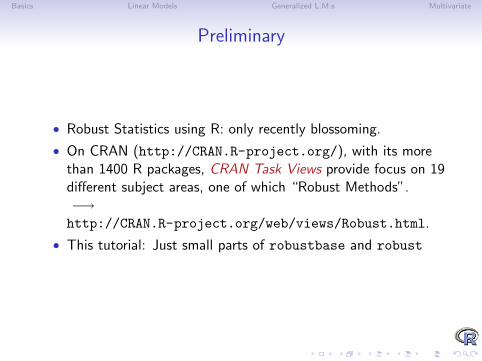
Preliminary
• Robust Statistics using R: only recently blossoming.
• On CRAN (http://CRAN.R-project.org/), with its morethan 1400 R packages, CRAN Task Views provide focus on 19different subject areas, one of which “Robust Methods”.−→http://CRAN.R-project.org/web/views/Robust.html.
• This tutorial: Just small parts of robustbase and robust

Basics Linear Models Generalized L.M.s Multivariate
— Part 1 —

Basics Linear Models Generalized L.M.s Multivariate
Basics: Sensitivity-Curve
The sensitivity curve is the “empirical influence function”, i.e.,
SCn(...) n→∞→ IF (...)
SC(x;x1, . . . , xn−1;Tn) :=Tn(x1, . . . , xn−1, x)− Tn−1(x1, . . . , xn−1)
1/n= n · (Tn(x1, . . . , xn−1, x)− Tn−1(x1, . . . , xn−1)) .
Task: Compute and plot the SC() for a few location estimators(i.e., the arithmetic mean and robust versions of it).
Basics Linear Models Generalized L.M.s Multivariate
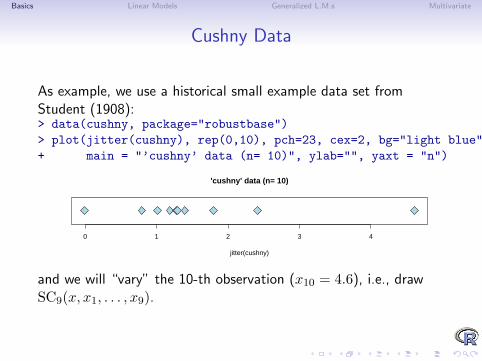
Cushny Data
As example, we use a historical small example data set fromStudent (1908):> data(cushny, package="robustbase")> plot(jitter(cushny), rep(0,10), pch=23, cex=2, bg="light blue",+ main = "’cushny’ data (n= 10)", ylab="", yaxt = "n")
0 1 2 3 4
'cushny' data (n= 10)
jitter(cushny)
and we will “vary” the 10-th observation (x10 = 4.6), i.e., drawSC9(x, x1, . . . , x9).

Basics Linear Models Generalized L.M.s Multivariate
SC ()
In the accompanying R-script,we define a short function SC() tocompute the sensitivity curve; it is basically
1 SC <− funct ion ( x , x . dat , EST , . . . ){
3 # Arguments : x : v a r y i n g data po i n t − as v e c t o r !# x . dat : the n−1 g i v en x 1 . . x n
5 # EST : f u n c t i o n ( x , . . . ) {x := ” sample ”}# . . . : o p t i o n a l f u r t h e r a rg . s to EST( )
7
s t o p i f n o t ( i s . numeric ( x ) , i s . numeric ( x . dat ) , i s . funct ion (EST ) )9 n 1 <− length ( x . dat )
n <− n 1 + 111 # when ’ x ’ i s a vec to r , compute T n ( x [ i ] , . . . ) f o r each one :
Tn <− sapply ( x , funct ion ( z ) EST( c ( x . dat , z ) , . . . ) )13 n∗ (Tn − EST( x . dat , . . . ) )}
Basics Linear Models Generalized L.M.s Multivariate
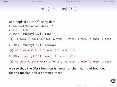
SC (., cushny[-10])
and applied to the Cushny data,> source("R/basics-defs.R")> x <- -1:6> SC(x, cushny[-10], mean)
[1] -2.2444 -1.2444 -0.2444 0.7556 1.7556 2.7556 3.7556 4.7556
> SC(x, cushny[-10], median)
[1] -0.5 -0.5 -0.5 0.0 0.0 0.0 0.0 0.0
> SC(x, cushny[-10], mean, trim = 0.20)
[1] -0.9048 -0.9048 -0.5714 0.7619 0.7619 0.7619 0.7619 0.7619
we see that the SC() function is linear for the mean and boundedfor the median and a trimmed mean.
Basics Linear Models Generalized L.M.s Multivariate
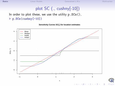
plot SC (., cushny[-10])In order to plot these, we use the utility p.SCs(),> p.SCs(cushny[-10])
−1 0 1 2 3
−2
−1
01
2
Sensitivity Curves SC(.) for location estimates
x
SC
(x, *
)
MeanMedianHubMHubp2

Basics Linear Models Generalized L.M.s Multivariate
plot SC (., cushny[-10]) — 2
p.SCs(., *) uses by default the following to versions of Huberlocation M-estimators, both of which behave remarkably. 1
## huber s ( ) i s i n MASS −− computing ‘ ‘ p r o p o s a l 2 ’ ’2 HubS <− funct ion ( x , . . . ) h u b e r s ( x , . . . ) $mu
4 ## huberM ( ) i s i n r obu s t b a s e −− and r e t u r n s a s h o r t l i s t − need on l y ’mu ’ :HubM <− funct ion ( x , . . . ) huberM ( x , . . . ) $mu
1We need these definitions here because the corresponding functions inMASS and robustbase return a list structure.
Basics Linear Models Generalized L.M.s Multivariate
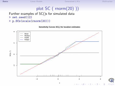
plot SC ( rnorm(20) ))Further examples of SC()s for simulated data> set.seed(12)> p.SCs(scale(rnorm(20)))
−2 0 2 4
−2
02
4
Sensitivity Curves SC(.) for location estimates
x
SC
(x, *
)
MeanMedianHubMHubp2
Basics Linear Models Generalized L.M.s Multivariate
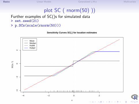
plot SC ( rnorm(50) ))Further examples of SC()s for simulated data> set.seed(21)> p.SCs(scale(rnorm(50)))
−4 −2 0 2
−4
−2
02
Sensitivity Curves SC(.) for location estimates
x
SC
(x, *
)
MeanMedianHubMHubp2
Basics Linear Models Generalized L.M.s Multivariate
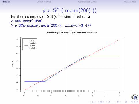
plot SC ( rnorm(200) ))Further examples of SC()s for simulated data> set.seed(1959)> p.SCs(scale(rnorm(200)), xlim=c(-3,4))
−3 −2 −1 0 1 2 3 4
−3
−2
−1
01
23
4
Sensitivity Curves SC(.) for location estimates
x
SC
(x, *
)
MeanMedianHubMHubp2
Basics Linear Models Generalized L.M.s Multivariate
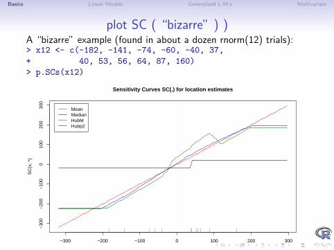
plot SC ( “bizarre” ) )A “bizarre” example (found in about a dozen rnorm(12) trials):> x12 <- c(-182, -141, -74, -60, -40, 37,+ 40, 53, 56, 64, 87, 160)> p.SCs(x12)
−300 −200 −100 0 100 200 300
−30
0−
200
−10
00
100
200
300
Sensitivity Curves SC(.) for location estimates
x
SC
(x, *
)
MeanMedianHubMHubp2

Basics Linear Models Generalized L.M.s Multivariate
Questions on Section 1 — “Basics” ?

Basics Linear Models Generalized L.M.s Multivariate
— Part 2 —
Basics Linear Models Generalized L.M.s Multivariate
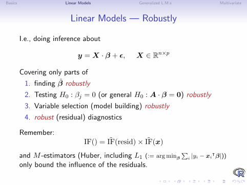
Linear Models — Robustly
I.e., doing inference about
y = X · β + ε, X ∈ Rn×p
Covering only parts of
1. finding β robustly
2. Testing H0 : βj = 0 (or general H0 : A · β = 0) robustly
3. Variable selection (model building) robustly
4. robust (residual) diagnostics
Remember:IF() = IF(resid)× IF(x)
and M -estimators (Huber, including L1 (:= arg minβ
Pi |yi − xi
ᵀβ|))
only bound the influence of the residuals.
Basics Linear Models Generalized L.M.s Multivariate
Robust LM with R
R: Standard lm() is for classical least squares. “Robust lm” inthree flavors:
• rlm() from MASS1
• lmrob() from robustbase
• lmRob() from robust (Insightful)
1MASS = “Recommended” R package: always installed
Basics Linear Models Generalized L.M.s Multivariate
Robust LM with R– Overview
“Exercise tasks”:
1. Get a feeling for robust “simple” regression, p = 2,xi = (1, xi) ∈ R2.
−→ interactive demo.
2. Main importance of robust regression is not for p = 2, butrather p ≈ 10, 20, 50 or even higher!
Basics Linear Models Generalized L.M.s Multivariate
Robust Simple LM with R
“Simple” regression: p = 2 :
yi = β1 + β2xi + εi.
1. Artificial example (residual plots in lecture notes ≈ p.37)
2. interactive “play” and demo
Basics Linear Models Generalized L.M.s Multivariate
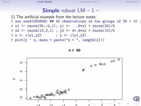
Simple robust LM – 1 –1) The artificial example from the lecture notes:> set.seed(050808) ## 40 observations in two groups of 30 + 10 :> x1 <- rnorm(30,-2,1); y1 <- .6*x1 + rnorm(30)/5> x2 <- rnorm(10,2,1) ; y2 <- 4+.8*x2 + rnorm(10)/5> x <- c(x1,x2) ; y <- c(y1,y2)> plot(y ~ x, main = paste("n = ", length(x)))
●
●
●
●●
●
●●
●●
●●
●
●●
●●
●
●
●
● ●
●
●●●
●
●
●
●
●
●
●
●
●
●
●
●
●
●
−3 −2 −1 0 1 2 3
−2
02
46
n = 40
x
y
−→ Which lines are which ?
Basics Linear Models Generalized L.M.s Multivariate
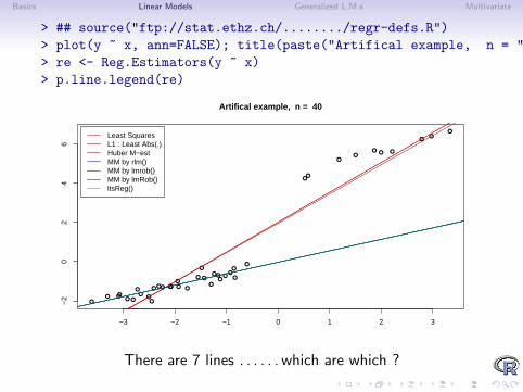
> ## source("ftp://stat.ethz.ch/......../regr-defs.R")> plot(y ~ x, ann=FALSE); title(paste("Artifical example, n = ",length(x)))> re <- Reg.Estimators(y ~ x)> p.line.legend(re)
●
●
●
●●
●
● ●
●
●
●
●
●
●
●●
●
●
●
●
● ●
●
●●●
●
●
●
●
●
●
●
●
●
●
●
●
●
●
−3 −2 −1 0 1 2 3
−2
02
46
Artifical example, n = 40
Least SquaresL1 : Least Abs(.)Huber M−estMM by rlm()MM by lmrob()MM by lmRob()ltsReg()
There are 7 lines . . . . . . which are which ?
Basics Linear Models Generalized L.M.s Multivariate
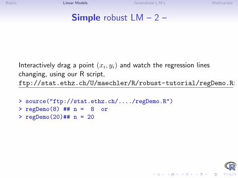
Simple robust LM – 2 –
Interactively drag a point (xi, yi) and watch the regression lineschanging, using our R script,ftp://stat.ethz.ch/U/maechler/R/robust-tutorial/regDemo.R:
> source("ftp://stat.ethz.ch/..../regDemo.R")> regDemo(8) ## n = 8 or> regDemo(20)## n = 20
Basics Linear Models Generalized L.M.s Multivariate
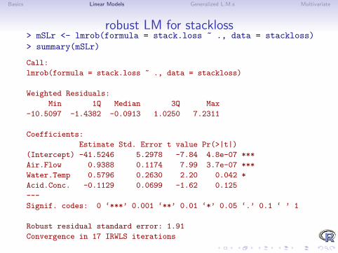
robust LM for stackloss> mSLr <- lmrob(formula = stack.loss ~ ., data = stackloss)> summary(mSLr)
Call:
lmrob(formula = stack.loss ~ ., data = stackloss)
Weighted Residuals:
Min 1Q Median 3Q Max
-10.5097 -1.4382 -0.0913 1.0250 7.2311
Coefficients:
Estimate Std. Error t value Pr(>|t|)
(Intercept) -41.5246 5.2978 -7.84 4.8e-07 ***
Air.Flow 0.9388 0.1174 7.99 3.7e-07 ***
Water.Temp 0.5796 0.2630 2.20 0.042 *
Acid.Conc. -0.1129 0.0699 -1.62 0.125
---
Signif. codes: 0 ‘***’ 0.001 ‘**’ 0.01 ‘*’ 0.05 ‘.’ 0.1 ‘ ’ 1
Robust residual standard error: 1.91
Convergence in 17 IRWLS iterations
Robustness weights:
observation 21 is an outlier with |weight| = 0 ( < 0.0048);
2 weights are ~= 1. The remaining 18 ones are summarized as
Min. 1st Qu. Median Mean 3rd Qu. Max.
0.122 0.876 0.943 0.872 0.980 0.998
Algorithmic parameters:
tuning.chi bb tuning.psi refine.tol rel.tol
1.55e+00 5.00e-01 4.69e+00 1.00e-07 1.00e-07
nResample max.it groups n.group best.r.s k.fast.s k.max
500 50 5 400 2 1 200
trace.lev compute.rd
0 0
seed : int(0)
Basics Linear Models Generalized L.M.s Multivariate
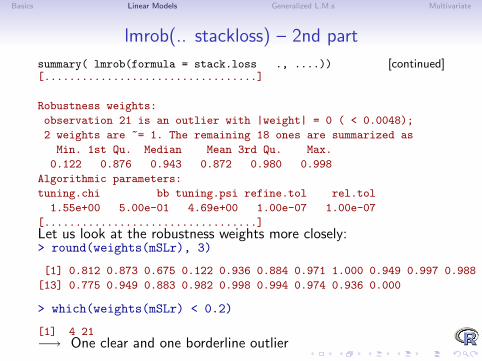
lmrob(.. stackloss) – 2nd part
summary( lmrob(formula = stack.loss ., ....)) [continued][..................................]
Robustness weights:
observation 21 is an outlier with |weight| = 0 ( < 0.0048);
2 weights are ~= 1. The remaining 18 ones are summarized as
Min. 1st Qu. Median Mean 3rd Qu. Max.
0.122 0.876 0.943 0.872 0.980 0.998
Algorithmic parameters:
tuning.chi bb tuning.psi refine.tol rel.tol
1.55e+00 5.00e-01 4.69e+00 1.00e-07 1.00e-07
[..................................]Let us look at the robustness weights more closely:> round(weights(mSLr), 3)
[1] 0.812 0.873 0.675 0.122 0.936 0.884 0.971 1.000 0.949 0.997 0.988 0.999
[13] 0.775 0.949 0.883 0.982 0.998 0.994 0.974 0.936 0.000
> which(weights(mSLr) < 0.2)
[1] 4 21−→ One clear and one borderline outlier
Basics Linear Models Generalized L.M.s Multivariate
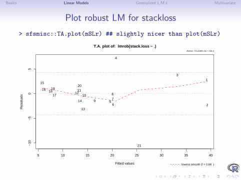
Plot robust LM for stackloss
> sfsmisc::TA.plot(mSLr) ## slightly nicer than plot(mSLr)
5 10 15 20 25 30 35 40
−10
−5
05
T.A. plot of: lmrob(stack.loss ~ .)
Fitted values
Res
idua
ls
1
2
3
4
56
7
8
9
10
1112
13
14
15
16
1718
1920
21
sfsmisc::TA.plot(lm.res = mSLr)
−.−.−.− : lowess smooth (f = 0.68 )
Basics Linear Models Generalized L.M.s Multivariate
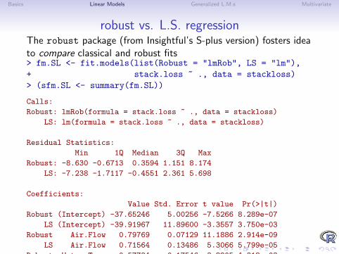
robust vs. L.S. regressionThe robust package (from Insightful’s S-plus version) fosters ideato compare classical and robust fits> fm.SL <- fit.models(list(Robust = "lmRob", LS = "lm"),+ stack.loss ~ ., data = stackloss)> (sfm.SL <- summary(fm.SL))
Calls:
Robust: lmRob(formula = stack.loss ~ ., data = stackloss)
LS: lm(formula = stack.loss ~ ., data = stackloss)
Residual Statistics:
Min 1Q Median 3Q Max
Robust: -8.630 -0.6713 0.3594 1.151 8.174
LS: -7.238 -1.7117 -0.4551 2.361 5.698
Coefficients:
Value Std. Error t value Pr(>|t|)
Robust (Intercept) -37.65246 5.00256 -7.5266 8.289e-07
LS (Intercept) -39.91967 11.89600 -3.3557 3.750e-03
Robust Air.Flow 0.79769 0.07129 11.1886 2.914e-09
LS Air.Flow 0.71564 0.13486 5.3066 5.799e-05
Robust Water.Temp 0.57734 0.17546 3.2905 4.318e-03
LS Water.Temp 1.29529 0.36802 3.5196 2.630e-03
Robust Acid.Conc. -0.06706 0.06512 -1.0297 3.176e-01
LS Acid.Conc. -0.15212 0.15629 -0.9733 3.440e-01
Residual Scale Estimates:
Robust: 1.837 on 17 degrees of freedom
LS: 3.243 on 17 degrees of freedom
Multiple R-Squared:
Robust: 0.6205
LS: 0.9136
Bias Tests for Robust Models:
Robust:
statistic p-value
M-estimate 2.751 0.6004
LS-estimate 2.640 0.6197
Basics Linear Models Generalized L.M.s Multivariate
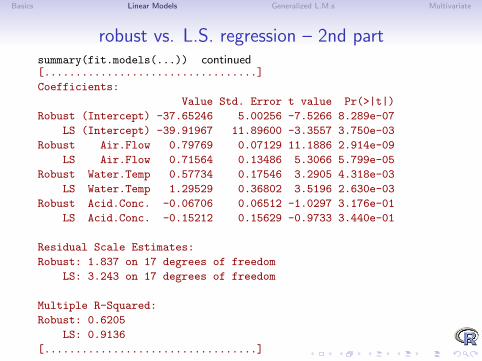
robust vs. L.S. regression – 2nd partsummary(fit.models(...)) continued[..................................]
Coefficients:
Value Std. Error t value Pr(>|t|)
Robust (Intercept) -37.65246 5.00256 -7.5266 8.289e-07
LS (Intercept) -39.91967 11.89600 -3.3557 3.750e-03
Robust Air.Flow 0.79769 0.07129 11.1886 2.914e-09
LS Air.Flow 0.71564 0.13486 5.3066 5.799e-05
Robust Water.Temp 0.57734 0.17546 3.2905 4.318e-03
LS Water.Temp 1.29529 0.36802 3.5196 2.630e-03
Robust Acid.Conc. -0.06706 0.06512 -1.0297 3.176e-01
LS Acid.Conc. -0.15212 0.15629 -0.9733 3.440e-01
Residual Scale Estimates:
Robust: 1.837 on 17 degrees of freedom
LS: 3.243 on 17 degrees of freedom
Multiple R-Squared:
Robust: 0.6205
LS: 0.9136
[..................................]

Basics Linear Models Generalized L.M.s Multivariate
Questions on Section 2 — “Linear Models” ?

Basics Linear Models Generalized L.M.s Multivariate
— Part 3 —
Basics Linear Models Generalized L.M.s Multivariate
Generalized Linear Models
We will only consider
• Logistic/Binomial regression
• Poisson regression (for count data)
Task: One GLM for each situation, including tests . . . . . .
Basics Linear Models Generalized L.M.s Multivariate
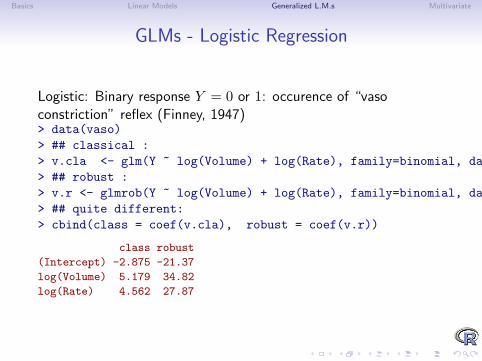
GLMs - Logistic Regression
Logistic: Binary response Y = 0 or 1: occurence of “vasoconstriction” reflex (Finney, 1947)> data(vaso)> ## classical :> v.cla <- glm(Y ~ log(Volume) + log(Rate), family=binomial, data=vaso)> ## robust :> v.r <- glmrob(Y ~ log(Volume) + log(Rate), family=binomial, data=vaso)> ## quite different:> cbind(class = coef(v.cla), robust = coef(v.r))
class robust
(Intercept) -2.875 -21.37
log(Volume) 5.179 34.82
log(Rate) 4.562 27.87

Basics Linear Models Generalized L.M.s Multivariate
GLMs - Logistic – 2 –We can do inference: classical and robust> summary(v.cla)# indication of clear effect
Call:
glm(formula = Y ~ log(Volume) + log(Rate), family = binomial,
data = vaso)
Deviance Residuals:
Min 1Q Median 3Q Max
-1.453 -0.611 0.100 0.618 2.278
Coefficients:
Estimate Std. Error z value Pr(>|z|)
(Intercept) -2.88 1.32 -2.18 0.0295 *
log(Volume) 5.18 1.86 2.78 0.0055 **
log(Rate) 4.56 1.84 2.48 0.0131 *
---
Signif. codes: 0 ‘***’ 0.001 ‘**’ 0.01 ‘*’ 0.05 ‘.’ 0.1 ‘ ’ 1
(Dispersion parameter for binomial family taken to be 1)
Null deviance: 54.040 on 38 degrees of freedom
Residual deviance: 29.227 on 36 degrees of freedom
AIC: 35.23
Number of Fisher Scoring iterations: 6
Basics Linear Models Generalized L.M.s Multivariate
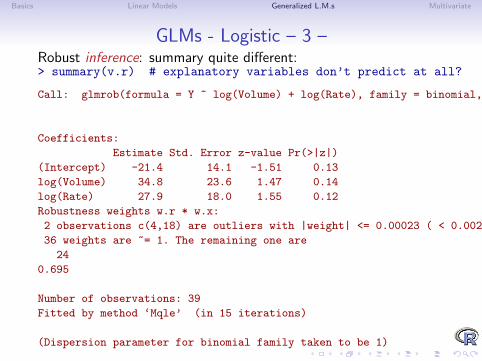
GLMs - Logistic – 3 –Robust inference: summary quite different:> summary(v.r) # explanatory variables don’t predict at all?
Call: glmrob(formula = Y ~ log(Volume) + log(Rate), family = binomial, data = vaso)
Coefficients:
Estimate Std. Error z-value Pr(>|z|)
(Intercept) -21.4 14.1 -1.51 0.13
log(Volume) 34.8 23.6 1.47 0.14
log(Rate) 27.9 18.0 1.55 0.12
Robustness weights w.r * w.x:
2 observations c(4,18) are outliers with |weight| <= 0.00023 ( < 0.0026);
36 weights are ~= 1. The remaining one are
24
0.695
Number of observations: 39
Fitted by method ‘Mqle’ (in 15 iterations)
(Dispersion parameter for binomial family taken to be 1)
No deviance values available
Algorithmic parameters:
acc tcc
0.0001 1.3450
maxit
50
test.acc
"coef"
Basics Linear Models Generalized L.M.s Multivariate
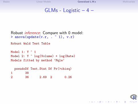
GLMs - Logistic – 4 –
Robust inference: Compare with 0 model:> anova(update(v.r, . ~ 1), v.r)
Robust Wald Test Table
Model 1: Y ~ 1
Model 2: Y ~ log(Volume) + log(Rate)
Models fitted by method ’Mqle’
pseudoDf Test.Stat Df Pr(>chisq)
1 38
2 36 2.69 2 0.26
Basics Linear Models Generalized L.M.s Multivariate
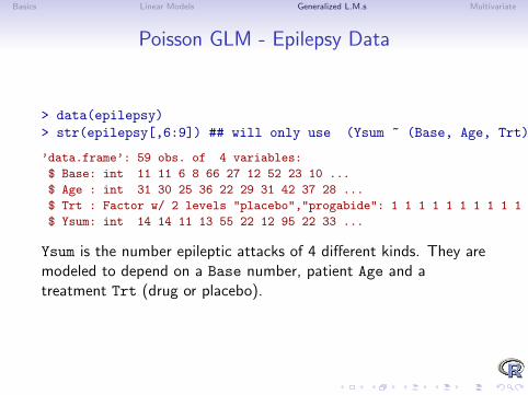
Poisson GLM - Epilepsy Data
> data(epilepsy)> str(epilepsy[,6:9]) ## will only use (Ysum ~ (Base, Age, Trt))
’data.frame’: 59 obs. of 4 variables:
$ Base: int 11 11 6 8 66 27 12 52 23 10 ...
$ Age : int 31 30 25 36 22 29 31 42 37 28 ...
$ Trt : Factor w/ 2 levels "placebo","progabide": 1 1 1 1 1 1 1 1 1 1 ...
$ Ysum: int 14 14 11 13 55 22 12 95 22 33 ...
Ysum is the number epileptic attacks of 4 different kinds. They aremodeled to depend on a Base number, patient Age and atreatment Trt (drug or placebo).
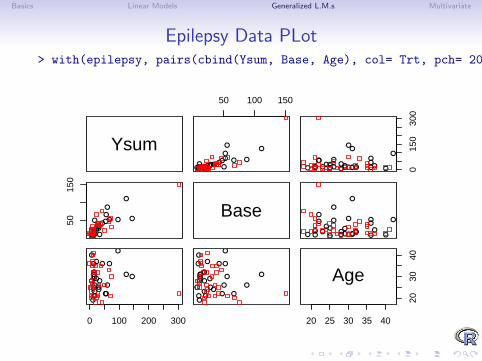
Basics Linear Models Generalized L.M.s Multivariate
Epilepsy Data PLot> with(epilepsy, pairs(cbind(Ysum, Base, Age), col= Trt, pch= 20+as.integer(Trt)))
Ysum
50 100 150
●●●●
●●●
●
●●●
●●●
●
●●
●
●●●●●●
●
●●
●
015
030
0
●●● ●
●● ●
●
●●●
●●●
●
● ●
●
●● ●● ●●
●
●●
●
5015
0
●●●●
●
●●
●
●●
●
●●
●
●
●
●
●
●●●●●
●
●
●●
●
Base●●● ●
●
●●
●
●●
●
●●
●
●
●
●
●
●●●●
●●
●
●●
●
0 100 200 300
●●
●
●
●
●●
●
●
●
●
●●
●
●●●
●●
●
●
●
●
●
●
●
●●
●●
●
●
●
●●
●
●
●
●
●●
●
●●●
●●
●
●
●
●
●
●
●
●●
20 25 30 35 40
2030
40
Age

Basics Linear Models Generalized L.M.s Multivariate
GLMs - Poisson Regression> summary(m1 <- glmrob(Ysum ~ Age + Base*Trt, family=poisson, data=epilepsy))
Call: glmrob(formula = Ysum ~ Age + Base * Trt, family = poisson, data = epilepsy)
Coefficients:
Estimate Std. Error z-value Pr(>|z|)
(Intercept) 2.04495 0.15217 13.44 < 2e-16 ***
Age 0.01600 0.00468 3.42 0.00064 ***
Base 0.02124 0.00103 20.64 < 2e-16 ***
Trtprogabide -0.33278 0.08630 -3.86 0.00012 ***
Base:Trtprogabide 0.00299 0.00123 2.44 0.01462 *
---
Signif. codes: 0 ‘***’ 0.001 ‘**’ 0.01 ‘*’ 0.05 ‘.’ 0.1 ‘ ’ 1
Robustness weights w.r * w.x:
27 weights are ~= 1. The remaining 32 ones are summarized as
Min. 1st Qu. Median Mean 3rd Qu. Max.
0.0829 0.3440 0.5620 0.5380 0.7610 0.9640
Number of observations: 59
Fitted by method ‘Mqle’ (in 13 iterations)
(Dispersion parameter for poisson family taken to be 1)
No deviance values available
Algorithmic parameters:
acc tcc
0.0001 1.3450
maxit
50
test.acc
"coef"
Basics Linear Models Generalized L.M.s Multivariate
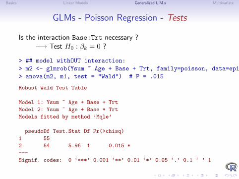
GLMs - Poisson Regression - Tests
Is the interaction Base:Trt necessary ?−→ Test H0 : βk = 0 ?
> ## model withOUT interaction:> m2 <- glmrob(Ysum ~ Age + Base + Trt, family=poisson, data=epilepsy)> anova(m2, m1, test = "Wald") # P = .015
Robust Wald Test Table
Model 1: Ysum ~ Age + Base + Trt
Model 2: Ysum ~ Age + Base * Trt
Models fitted by method ’Mqle’
pseudoDf Test.Stat Df Pr(>chisq)
1 55
2 54 5.96 1 0.015 *
---
Signif. codes: 0 ‘***’ 0.001 ‘**’ 0.01 ‘*’ 0.05 ‘.’ 0.1 ‘ ’ 1
Basics Linear Models Generalized L.M.s Multivariate
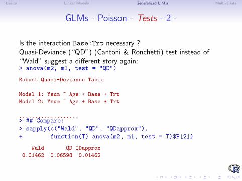
GLMs - Poisson - Tests - 2 -
Is the interaction Base:Trt necessary ?Quasi-Deviance (“QD”) (Cantoni & Ronchetti) test instead of“Wald” suggest a different story again:> anova(m2, m1, test = "QD")
Robust Quasi-Deviance Table
Model 1: Ysum ~ Age + Base + Trt
Model 2: Ysum ~ Age + Base * Trt
...................> ## Compare:> sapply(c("Wald", "QD", "QDapprox"),+ function(T) anova(m2, m1, test = T)$P[2])
Wald QD QDapprox
0.01462 0.06598 0.01462

Basics Linear Models Generalized L.M.s Multivariate
Questions on Section 3 — “Generalized LM’s” ?

Basics Linear Models Generalized L.M.s Multivariate
— Part 4 —
Basics Linear Models Generalized L.M.s Multivariate
Multivariate Location & Scatter
Estimation “location” and “scatter” in p-dimensional, e.g.,estimation of µ and Σ.Tasks: similar to regression,
1. p = 2 is “easy”, and nice for visualization
2. For p ≥ 3, and “p moderately large”, robustness is harder toachieve and more important
Basics Linear Models Generalized L.M.s Multivariate
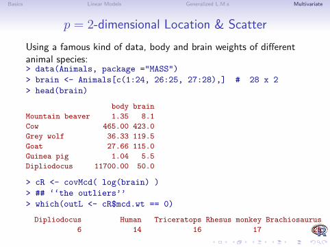
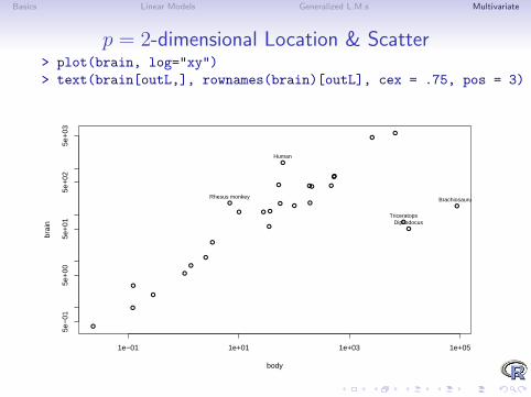
p = 2-dimensional Location & Scatter
Using a famous kind of data, body and brain weights of differentanimal species:> data(Animals, package ="MASS")> brain <- Animals[c(1:24, 26:25, 27:28),] # 28 x 2> head(brain)
body brain
Mountain beaver 1.35 8.1
Cow 465.00 423.0
Grey wolf 36.33 119.5
Goat 27.66 115.0
Guinea pig 1.04 5.5
Dipliodocus 11700.00 50.0
> cR <- covMcd( log(brain) )> ## ‘‘the outliers’’> which(outL <- cR$mcd.wt == 0)
Dipliodocus Human Triceratops Rhesus monkey Brachiosaurus
6 14 16 17 25
Basics Linear Models Generalized L.M.s Multivariate
p = 2-dimensional Location & Scatter> plot(brain, log="xy")> text(brain[outL,], rownames(brain)[outL], cex = .75, pos = 3)
●
●
●●
●
●
●
●
●
●
●
●
●
●
●
●
●
●
●
●
●
● ●
●
●
●
●
●
1e−01 1e+01 1e+03 1e+05
5e−
015e
+00
5e+
015e
+02
5e+
03
body
brai
n Dipliodocus
Human
Triceratops
Rhesus monkey Brachiosaurus
Basics Linear Models Generalized L.M.s Multivariate
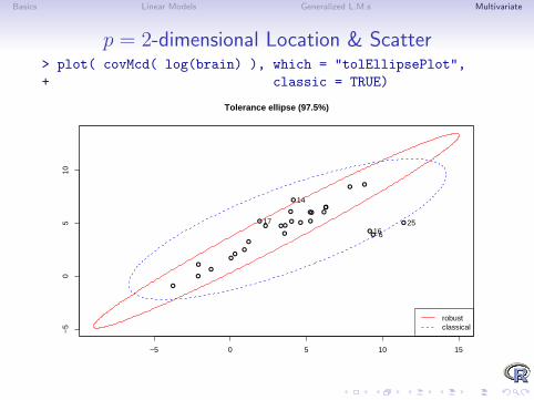
p = 2-dimensional Location & Scatter> plot( covMcd( log(brain) ), which = "tolEllipsePlot",+ classic = TRUE)
●
●
●●
●
●
●
●●
●
●
●●
●
●
●
●
●
●
●
●
● ●
●
●
●●
●
−5 0 5 10 15
−5
05
10
Tolerance ellipse (97.5%)
17
14
166
25
robustclassical
Basics Linear Models Generalized L.M.s Multivariate
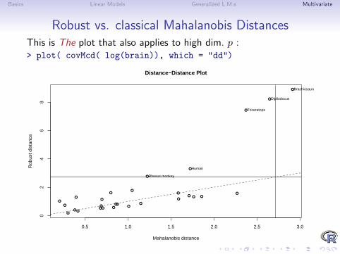
Robust vs. classical Mahalanobis DistancesThis is The plot that also applies to high dim. p :> plot( covMcd( log(brain)), which = "dd")
●
●
●●
●
●
●
●
●
●
●●
●
●
●
●
●
●
●●
●●
●
●
●
●
●
●
0.5 1.0 1.5 2.0 2.5 3.0
02
46
8
Distance−Distance Plot
Mahalanobis distance
Rob
ust d
ista
nce
Brachiosaurus
Dipliodocus
Triceratops
Human
Rhesus monkey
Basics Linear Models Generalized L.M.s Multivariate
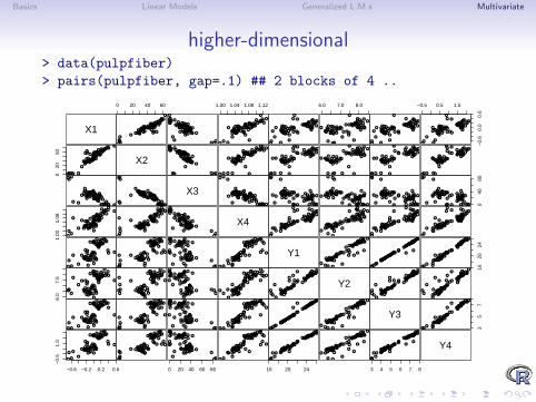
higher-dimensional> data(pulpfiber)> pairs(pulpfiber, gap=.1) ## 2 blocks of 4 ..
X1
0 20 40 60
●●●●●●
●●
● ●●
●
●● ●
●●
●
●●● ●●
●
●●
●● ●●● ●
●●●●
●●
●●●●
●●
●●●●
●●
●●●●
●
●
●●
●●●
●
●●●●●●
●●
●●●
●
●●●●
●●
●●●● ●
●
●●
●●● ● ●●
●● ● ●
●●
●●
● ●●●
●● ●●
●●●●●●●
●
●●
●●
●●
1.00 1.04 1.08 1.12
●●●●●●
●●●●
●●
●●●
●●
●
●●●●●
●
●●
●● ●●●●
●●●●
●●
●●● ●
●●●
●●●
●●
● ●●
●●
●
●●
●●
●●
●●●●●●
●●
●●●
●
●●●
●●
●
●● ●● ●●
●●
●● ●●●●
●● ●●
●●
●●
●●●
●●
● ●●
●●
●●●
●●
●
●●●
●●
●
6.0 7.0 8.0
●●●●●●
●●
●●●
●
●●●
●●
●
●● ●● ●
●
●●
●● ●●● ●
●●● ●
●●
●●
● ●●
●●
● ●●
●●
●●●
●●
●
●●
●●
●●
●●●●●●
●●
●●●
●
●●●
●●
●
●● ●● ●●
●●
●● ●●●●
●● ● ●
●●
●●
●●●
●●
● ●●
●●
●●●
●●
●
●●●
●●
●
−0.5 0.5 1.5
−0.
60.
00.
6
●●●●● ●
●●
●●●
●
●●●
●●
●
●●●● ●
●
●●
●● ●●●●
●●●●
●●●
●●●
●●●
●●●
●●
●●●
●●
●
●●
●●
●●
020
50
●●●●
●●●●
●●
●●
● ●●
●●
●● ●●●●●
●●
●●●●●●
●
●●●●●●
●●● ●●●
●●●
●●●●●●●
●
●●● ● ●
●
X2 ●●●●
●●●●
●●
●●
●●●
●●
●●●●●
●●
●●
●●●
● ●●
●
●● ●
●● ●●●
●●● ●●
●●
●●●●●●●
●
● ●●●●
●
●●●●
●●●●
●●
●●●●●
●●
● ●●●●●●
●●
●●●
●●●
●
●●●
●● ●●●
●●●●●●●
●●● ●●●●
●
●●● ●●
●
●●●●
●●●●
●●●
●●●
●
●●
● ●● ●●
● ●
●●
●●●●●
●
●
●●●●● ●
● ●●● ●●
●●●
●●●● ●●●
●
●●● ●●
●
●●●●●●●
●
●●
●●●●
●
●●
● ● ● ●●
●●
●●
●●●●●
●
●
●● ●●● ●
● ●●● ●●
●●●
●●●● ●●●
●
●● ● ●●
●
●●●●
●●●●
●●●
●●●
●
●●
● ●● ●●
● ●
●●
●●●
●●●
●
●● ●●● ●
● ●●● ●●
●●●
●●●● ●●●
●
●●● ●●
●
●●●●
● ●●●
●●
●●
●●●
●●
● ●●●●
●●
●●
●●●●●
●
●
●●●●●●
●●●●●●
●●●
●●●● ●●●
●
●●● ●●
●
●●●●
●●●
●
●●
●●
● ●●
●●
●● ●●●●●
●●
●●●●
●●
●
●●
●●
●
●
●●●
●●●
●●●
●● ●●●●● ●
●●●
● ●
●●●
●●
●●●●
●●
●●
●●●
●●
●●●● ●●●
●●
●●●
●●
●
●
●●●
●●
●
●●●
●●●
●●●
●● ●●●●● ●
●●●
●●
●X3 ●●
●●
●●●
●
●●
●●●●●
●●
● ●●●●
●●
●●
●●●
●●●
●
●●●
●●
●
●●●
●●●
●●●
●●● ●●●●●
●●●
●●
●●●
●●
●●●●
●●●
●●●
●●
●
● ●●●●
● ●
●●
●●●●
●●
●
●●
●●●
●
● ●●
● ●●
●●●
●●●● ●●●●
●●●
●●
●●●
●●
●●●●
●●
●●●●
●●
●
● ● ● ●●●●
●●
●●●●
●●
●
●●
●●
●
●
● ●●
● ●●
●●●
●● ●● ●●●●
●● ●
●●
●●●
●●
●●●●
●●●
●●●
●●
●
● ●●●●
● ●
●●
●●●
●●
●
●
●●
●●●
●
● ●●
● ●●
●●●
●● ●● ●●●●
●●●
●●
●
040
80
●●●
●
● ●●●
●●
●●
●●●●
●
● ●●●●●●
●●
●●●●
●●
●
●●
●●●
●
●●●
●●●
●●●
●●●● ●●●●
●●●
●●
●
1.00
1.08
●●●●●●● ●●●
●● ● ●
●●●●
● ●●
●●●
● ●●
●
●●●●
●
●●●
●●●
●●●
●●●●●●
●● ●●
●●
● ●
●●
●
●
●
●●●●●●●
● ●● ●●
● ●●●
●●●
●●●
●●●
● ●●
●
●●● ●
●
●●●
●●●
●●●
●●●
●●●
●● ●●
●●
● ●
●●
●
●
●
●●●●● ●●●● ●●
●●●●
●● ●
●
●●●
● ●●
●● ●
●
● ●●●
●
● ● ●
●●●
●●●
●●●
● ●●
●●●●●●●●
●●
●
●
●
● X4 ●●●● ●●●● ●●
●●●●
●●●
●
●●●
● ● ●
● ● ●
●
●●●●
●
● ●●
●●●
● ●●
● ●●● ●●
●●●●
●●●●
●●●
●
●
●●●●● ●●
●● ●●●
●●●●
● ●●
● ●●
● ●●
● ● ●
●
●●● ●
●
●● ●
●●●
● ●●
● ●●● ●●
●● ●●
●●
●●
●●
●
●
●
●●●●● ●●
●● ●●●
●●●●
● ●●
●●●
● ● ●
● ● ●
●
●●●●
●
● ● ●
●●●
● ●●
● ●●● ●●
●● ●●
●●●●
●●●
●
●
●●●●●● ●
●● ●●●
●●●●●●
●
●●●
● ●●
●●●
●
●●●●
●
●●●
●●●
●●●
●●●●●●
●●●●
●●●●
●●
●
●
●
●
●●●●
●●
● ●●
● ●● ●
●●●●
●
● ●●
●
●●
●●
●
●
●●
●●●
●●
●●●
●●
●●
●●●
●●●
●●
●●
●●●
●
●
●●
●
●
●●●●
●●●
● ●●
● ●● ●
● ●●●
●
●●●
●
●●
●●
●
●
●●
●●●
●●●
●●●
●●●
●●●
●●●
●●
●●
●●●
●
●
●●
●
●
●●●●
●●●
●●●
●●●●
●● ●●
●
●●●
●
●●
●●
●
●
● ●
●● ●
●●
●●●
●●
● ●
●● ●
●●●
●●
●●
●●●
●
●
●●
●
●
●●●●
●●●
●●●● ●●●●●●
●
●
●●●
●
●●
●●
●
●
●●
●●●
●●●
●●●
●● ●
●●●
●●●
●●
●●
●●●
●
●
●●
●
●
● Y1 ●●●●
●●
●●●
●●●●
●●●●
●
● ●●
●
●●
●●
●
●
●●
●● ●
●●
●●●
●●
● ●
●●●
●●●
●●
●●
●●●
●
●
● ●
●
●
●●●●
●●●
●●●
●●●●
●●●●
●
●●●
●
●●
●●
●
●
●●
●● ●
●●
●●●
●●
●●
●●●
●●●
●●
●●
●●●
●
●
●●
●
●
●
1620
24
●●●●● ●
●●●
●●●●●●●●
●
●●●
●
●●
●●●
●
●●
●●●
●●
●●●
●●
●●
●●●
●●●
●●
●●
●●●
●
●
●●
●
●
●
6.0
7.5
●●●●
●●
●●
●●●
● ●●●●
●
●●
●
●
●
●●
●●
●
●
●●
●●
●
●●
●●●
●
●
●●
●
●●
●●●
●●
●
●
●●●
●
●
●●
●
●
●
●●●●
●●
●●
● ●●
● ●●
●●●
●●
●
●
●
●●
●●
●
●
●●
●●
●
●●●
●●
●
●
●●
●
●●
●●●
●●
●
●
●●●
●
●
●●
●
●
●
●●●
●●●
●●
●●●
●●●
● ●●
●●
●
●
●
●●
●●
●
●
● ●
●●
●
●●
●●●
●
●
●●
●
●●
●●●
●●
●
●
●●●
●
●
●●
●
●
●
●●●
●●●
●●●●
●
●●●
●●●
●●●
●
●
●●
●●
●
●
●●
●●
●
●●●
●●
●
●
●●
●
●●
●●●
●●
●
●
●●●
●
●
●●
●
●
●
●●●
●●●
●●
●●●
●●●
●●●
●●●
●
●
● ●
●●
●
●
●●
●●
●
●●
●●●
●
●
●●
●
●●
●●●
●●
●
●
●●●
●
●
●●
●
●
● Y2 ●●●
●●●
●●
●●●
●●●
●●●
●●●
●
●
● ●
●●
●
●
●●
●●
●
●●
●●●
●
●
●●
●
●●
●●●
●●
●
●
●●●
●
●
●●
●
●
●
●●●
●● ●
●●
●●●
●●●
●●●
●●
●
●
●
●●
●●●
●
●●
●●
●
●●
●●●
●
●
●●
●
●●
●●●
●●
●
●
●●●
●
●
●●
●
●
●
●●●●
●●
● ●●
● ●● ●
●●●●
●
● ●●
●
●●
●●
●
●
●●
●●●
●●
●●●
●
●●●
●
●●
●●●
●●●
●
●●●
●
●
●●
●
●
●●●●
●●●
● ●●
● ●● ●
● ●●●
●
●●●
●
●●
●●
●
●
●●
● ●●
●●●
●●●
●●●
●
●●
●●●
●●●
●
●●●
●
●
●●
●
●
●●●●
●●●
●●●
●●●●
●● ●●
●
●●●
●
●●
●●
●
●
● ●
●●●
●●
●●●
●
●● ●
●
● ●
●●●
●●●
●
●●●
●
●
●●
●
●
●●●●
●●●
●●●● ●●●●●●
●
●
●●●
●
●●
●●
●
●
●●
●●●
●●●
●●●
●● ●
●
●●
●●●
●●●
●
●●●
●
●
●●
●
●
●●●●
●●●
●●●
●●●●
●●●●
●
●●●
●
●●
●●
●
●
●●
●●●
●●
●●●
●
●●●
●
●●
●●●
●●●
●
●●●
●
●
●●
●
●
●●●●
●●●
●●●
●●●●
●●●●
●
● ●●
●
●●
●●
●
●
●●
● ●●
●●
●●●
●
●● ●
●
●●
●●●
●●●
●
●●●
●
●
● ●
●
●
● Y3
35
7
●●●●● ●
●●●
●●●●●●●●
●
●●●
●
●●
●●●
●
●●
●●●
●●
●●●
●
●●●
●
●●
●●●
●●●
●
●●●
●
●
●●
●
●
●
−0.6 −0.2 0.2 0.6
−0.
51.
0
●●●●●
●
●●
●● ●
●●
●●●●
●● ●●
●●●
●●●
●●●
●●●●●
● ●●●●
●●●
●●
●●●
●●
●●
●●●
●
●
●●
●
●
●
●●●●●
●
●●
● ● ●
●●
● ●●●
●●●●
●●●
●●●
●●●
● ●●●●
●●●●
●●●
●●●
●●●
●●
●●
●●●
●
●
●●
●
●
●
0 20 40 60 80
●●●● ●
●
●●
●●●
●●●● ● ●
●●●●
●●●
●● ●
●● ●
●● ●● ●
● ●● ●●
● ●●● ●
●●●
●●
●●
●●●
●
●
●●
●
●
●
●●●●●●
●●●● ●
●●
●●●●
●●●
●
●●●
●●●
●●●
●●●
●●●●● ●
●● ●
●●●
●●●
●●
●●
●●●
●
●
●●
●
●
●
16 20 24
●●●● ●
●
●●
●●●
●●
●●●●
●●●
●
●● ●
●● ●
●●●
●●●● ●
●●●●
●●●
●●●
●●●
●●
●●
●●●
●
●
●●
●
●
●
●●●● ●
●
●●
●●●
●●
●●● ●
●● ● ●
●●●
●● ●
●●●
● ● ●●●
●●● ●●
● ●●
●●
●●●
●●
●●
●●●
●
●
● ●
●
●
●
3 4 5 6 7 8
●●●● ●
●
●●
●●●
●●
●●● ●
●●●
●
●● ●
●● ●
●●●
●● ●● ●
●●●●
●●●
●●●
●●●
●●
●●
●●●
●
●
●●
●
●
● Y4

Basics Linear Models Generalized L.M.s Multivariate
higher-dimensional> data(pulpfiber)> pairs(pulpfiber, gap=.1) ## 2 blocks of 4 ..
X1
0 20 40 60
●●●●●●
●●
● ●●
●
●● ●
●●
●
●●● ●●
●
●●
●● ●●● ●
●●●●
●●
●●●●
●●
●●●●
●●
●●●●
●
●
●●
●●●
●
●●●●●●
●●
●●●
●
●●●●
●●
●●●● ●
●
●●
●●● ● ●●
●● ● ●
●●
●●
● ●●●
●● ●●
●●●●●●●
●
●●
●●
●●
1.00 1.04 1.08 1.12
●●●●●●
●●●●
●●
●●●
●●
●
●●●●●
●
●●
●● ●●●●
●●●●
●●
●●● ●
●●●
●●●
●●
● ●●
●●
●
●●
●●
●●
●●●●●●
●●
●●●
●
●●●
●●
●
●● ●● ●●
●●
●● ●●●●
●● ●●
●●
●●
●●●
●●
● ●●
●●
●●●
●●
●
●●●
●●
●
6.0 7.0 8.0
●●●●●●
●●
●●●
●
●●●
●●
●
●● ●● ●
●
●●
●● ●●● ●
●●● ●
●●
●●
● ●●
●●
● ●●
●●
●●●
●●
●
●●
●●
●●
●●●●●●
●●
●●●
●
●●●
●●
●
●● ●● ●●
●●
●● ●●●●
●● ● ●
●●
●●
●●●
●●
● ●●
●●
●●●
●●
●
●●●
●●
●
−0.5 0.5 1.5
−0.
60.
00.
6
●●●●● ●
●●
●●●
●
●●●
●●
●
●●●● ●
●
●●
●● ●●●●
●●●●
●●●
●●●
●●●
●●●
●●
●●●
●●
●
●●
●●
●●
020
50
●●●●
●●●●
●●
●●
● ●●
●●
●● ●●●●●
●●
●●●●●●
●
●●●●●●
●●● ●●●
●●●
●●●●●●●
●
●●● ● ●
●
X2 ●●●●
●●●●
●●
●●
●●●
●●
●●●●●
●●
●●
●●●
● ●●
●
●● ●
●● ●●●
●●● ●●
●●
●●●●●●●
●
● ●●●●
●
●●●●
●●●●
●●
●●●●●
●●
● ●●●●●●
●●
●●●
●●●
●
●●●
●● ●●●
●●●●●●●
●●● ●●●●
●
●●● ●●
●
●●●●
●●●●
●●●
●●●
●
●●
● ●● ●●
● ●
●●
●●●●●
●
●
●●●●● ●
● ●●● ●●
●●●
●●●● ●●●
●
●●● ●●
●
●●●●●●●
●
●●
●●●●
●
●●
● ● ● ●●
●●
●●
●●●●●
●
●
●● ●●● ●
● ●●● ●●
●●●
●●●● ●●●
●
●● ● ●●
●
●●●●
●●●●
●●●
●●●
●
●●
● ●● ●●
● ●
●●
●●●
●●●
●
●● ●●● ●
● ●●● ●●
●●●
●●●● ●●●
●
●●● ●●
●
●●●●
● ●●●
●●
●●
●●●
●●
● ●●●●
●●
●●
●●●●●
●
●
●●●●●●
●●●●●●
●●●
●●●● ●●●
●
●●● ●●
●
●●●●
●●●
●
●●
●●
● ●●
●●
●● ●●●●●
●●
●●●●
●●
●
●●
●●
●
●
●●●
●●●
●●●
●● ●●●●● ●
●●●
● ●
●●●
●●
●●●●
●●
●●
●●●
●●
●●●● ●●●
●●
●●●
●●
●
●
●●●
●●
●
●●●
●●●
●●●
●● ●●●●● ●
●●●
●●
●X3 ●●
●●
●●●
●
●●
●●●●●
●●
● ●●●●
●●
●●
●●●
●●●
●
●●●
●●
●
●●●
●●●
●●●
●●● ●●●●●
●●●
●●
●●●
●●
●●●●
●●●
●●●
●●
●
● ●●●●
● ●
●●
●●●●
●●
●
●●
●●●
●
● ●●
● ●●
●●●
●●●● ●●●●
●●●
●●
●●●
●●
●●●●
●●
●●●●
●●
●
● ● ● ●●●●
●●
●●●●
●●
●
●●
●●
●
●
● ●●
● ●●
●●●
●● ●● ●●●●
●● ●
●●
●●●
●●
●●●●
●●●
●●●
●●
●
● ●●●●
● ●
●●
●●●
●●
●
●
●●
●●●
●
● ●●
● ●●
●●●
●● ●● ●●●●
●●●
●●
●
040
80
●●●
●
● ●●●
●●
●●
●●●●
●
● ●●●●●●
●●
●●●●
●●
●
●●
●●●
●
●●●
●●●
●●●
●●●● ●●●●
●●●
●●
●
1.00
1.08
●●●●●●● ●●●
●● ● ●
●●●●
● ●●
●●●
● ●●
●
●●●●
●
●●●
●●●
●●●
●●●●●●
●● ●●
●●
● ●
●●
●
●
●
●●●●●●●
● ●● ●●
● ●●●
●●●
●●●
●●●
● ●●
●
●●● ●
●
●●●
●●●
●●●
●●●
●●●
●● ●●
●●
● ●
●●
●
●
●
●●●●● ●●●● ●●
●●●●
●● ●
●
●●●
● ●●
●● ●
●
● ●●●
●
● ● ●
●●●
●●●
●●●
● ●●
●●●●●●●●
●●
●
●
●
● X4 ●●●● ●●●● ●●
●●●●
●●●
●
●●●
● ● ●
● ● ●
●
●●●●
●
● ●●
●●●
● ●●
● ●●● ●●
●●●●
●●●●
●●●
●
●
●●●●● ●●
●● ●●●
●●●●
● ●●
● ●●
● ●●
● ● ●
●
●●● ●
●
●● ●
●●●
● ●●
● ●●● ●●
●● ●●
●●
●●
●●
●
●
●
●●●●● ●●
●● ●●●
●●●●
● ●●
●●●
● ● ●
● ● ●
●
●●●●
●
● ● ●
●●●
● ●●
● ●●● ●●
●● ●●
●●●●
●●●
●
●
●●●●●● ●
●● ●●●
●●●●●●
●
●●●
● ●●
●●●
●
●●●●
●
●●●
●●●
●●●
●●●●●●
●●●●
●●●●
●●
●
●
●
●
●●●●
●●
● ●●
● ●● ●
●●●●
●
● ●●
●
●●
●●
●
●
●●
●●●
●●
●●●
●●
●●
●●●
●●●
●●
●●
●●●
●
●
●●
●
●
●●●●
●●●
● ●●
● ●● ●
● ●●●
●
●●●
●
●●
●●
●
●
●●
●●●
●●●
●●●
●●●
●●●
●●●
●●
●●
●●●
●
●
●●
●
●
●●●●
●●●
●●●
●●●●
●● ●●
●
●●●
●
●●
●●
●
●
● ●
●● ●
●●
●●●
●●
● ●
●● ●
●●●
●●
●●
●●●
●
●
●●
●
●
●●●●
●●●
●●●● ●●●●●●
●
●
●●●
●
●●
●●
●
●
●●
●●●
●●●
●●●
●● ●
●●●
●●●
●●
●●
●●●
●
●
●●
●
●
● Y1 ●●●●
●●
●●●
●●●●
●●●●
●
● ●●
●
●●
●●
●
●
●●
●● ●
●●
●●●
●●
● ●
●●●
●●●
●●
●●
●●●
●
●
● ●
●
●
●●●●
●●●
●●●
●●●●
●●●●
●
●●●
●
●●
●●
●
●
●●
●● ●
●●
●●●
●●
●●
●●●
●●●
●●
●●
●●●
●
●
●●
●
●
●
1620
24
●●●●● ●
●●●
●●●●●●●●
●
●●●
●
●●
●●●
●
●●
●●●
●●
●●●
●●
●●
●●●
●●●
●●
●●
●●●
●
●
●●
●
●
●
6.0
7.5
●●●●
●●
●●
●●●
● ●●●●
●
●●
●
●
●
●●
●●
●
●
●●
●●
●
●●
●●●
●
●
●●
●
●●
●●●
●●
●
●
●●●
●
●
●●
●
●
●
●●●●
●●
●●
● ●●
● ●●
●●●
●●
●
●
●
●●
●●
●
●
●●
●●
●
●●●
●●
●
●
●●
●
●●
●●●
●●
●
●
●●●
●
●
●●
●
●
●
●●●
●●●
●●
●●●
●●●
● ●●
●●
●
●
●
●●
●●
●
●
● ●
●●
●
●●
●●●
●
●
●●
●
●●
●●●
●●
●
●
●●●
●
●
●●
●
●
●
●●●
●●●
●●●●
●
●●●
●●●
●●●
●
●
●●
●●
●
●
●●
●●
●
●●●
●●
●
●
●●
●
●●
●●●
●●
●
●
●●●
●
●
●●
●
●
●
●●●
●●●
●●
●●●
●●●
●●●
●●●
●
●
● ●
●●
●
●
●●
●●
●
●●
●●●
●
●
●●
●
●●
●●●
●●
●
●
●●●
●
●
●●
●
●
● Y2 ●●●
●●●
●●
●●●
●●●
●●●
●●●
●
●
● ●
●●
●
●
●●
●●
●
●●
●●●
●
●
●●
●
●●
●●●
●●
●
●
●●●
●
●
●●
●
●
●
●●●
●● ●
●●
●●●
●●●
●●●
●●
●
●
●
●●
●●●
●
●●
●●
●
●●
●●●
●
●
●●
●
●●
●●●
●●
●
●
●●●
●
●
●●
●
●
●
●●●●
●●
● ●●
● ●● ●
●●●●
●
● ●●
●
●●
●●
●
●
●●
●●●
●●
●●●
●
●●●
●
●●
●●●
●●●
●
●●●
●
●
●●
●
●
●●●●
●●●
● ●●
● ●● ●
● ●●●
●
●●●
●
●●
●●
●
●
●●
● ●●
●●●
●●●
●●●
●
●●
●●●
●●●
●
●●●
●
●
●●
●
●
●●●●
●●●
●●●
●●●●
●● ●●
●
●●●
●
●●
●●
●
●
● ●
●●●
●●
●●●
●
●● ●
●
● ●
●●●
●●●
●
●●●
●
●
●●
●
●
●●●●
●●●
●●●● ●●●●●●
●
●
●●●
●
●●
●●
●
●
●●
●●●
●●●
●●●
●● ●
●
●●
●●●
●●●
●
●●●
●
●
●●
●
●
●●●●
●●●
●●●
●●●●
●●●●
●
●●●
●
●●
●●
●
●
●●
●●●
●●
●●●
●
●●●
●
●●
●●●
●●●
●
●●●
●
●
●●
●
●
●●●●
●●●
●●●
●●●●
●●●●
●
● ●●
●
●●
●●
●
●
●●
● ●●
●●
●●●
●
●● ●
●
●●
●●●
●●●
●
●●●
●
●
● ●
●
●
● Y3
35
7
●●●●● ●
●●●
●●●●●●●●
●
●●●
●
●●
●●●
●
●●
●●●
●●
●●●
●
●●●
●
●●
●●●
●●●
●
●●●
●
●
●●
●
●
●
−0.6 −0.2 0.2 0.6
−0.
51.
0
●●●●●
●
●●
●● ●
●●
●●●●
●● ●●
●●●
●●●
●●●
●●●●●
● ●●●●
●●●
●●
●●●
●●
●●
●●●
●
●
●●
●
●
●
●●●●●
●
●●
● ● ●
●●
● ●●●
●●●●
●●●
●●●
●●●
● ●●●●
●●●●
●●●
●●●
●●●
●●
●●
●●●
●
●
●●
●
●
●
0 20 40 60 80
●●●● ●
●
●●
●●●
●●●● ● ●
●●●●
●●●
●● ●
●● ●
●● ●● ●
● ●● ●●
● ●●● ●
●●●
●●
●●
●●●
●
●
●●
●
●
●
●●●●●●
●●●● ●
●●
●●●●
●●●
●
●●●
●●●
●●●
●●●
●●●●● ●
●● ●
●●●
●●●
●●
●●
●●●
●
●
●●
●
●
●
16 20 24
●●●● ●
●
●●
●●●
●●
●●●●
●●●
●
●● ●
●● ●
●●●
●●●● ●
●●●●
●●●
●●●
●●●
●●
●●
●●●
●
●
●●
●
●
●
●●●● ●
●
●●
●●●
●●
●●● ●
●● ● ●
●●●
●● ●
●●●
● ● ●●●
●●● ●●
● ●●
●●
●●●
●●
●●
●●●
●
●
● ●
●
●
●
3 4 5 6 7 8
●●●● ●
●
●●
●●●
●●
●●● ●
●●●
●
●● ●
●● ●
●●●
●● ●● ●
●●●●
●●●
●●●
●●●
●●
●●
●●●
●
●
●●
●
●
● Y4
Basics Linear Models Generalized L.M.s Multivariate
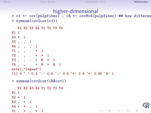
higher-dimensional> c1 <- cov(pulpfiber) ; cR <- covMcd(pulpfiber) ## how different are they..> symnum(cov2cor(c1))
X1 X2 X3 X4 Y1 Y2 Y3 Y4
X1 1
X2 * 1
X3 , , 1
X4 , , , 1
Y1 , , . + 1
Y2 . , . + * 1
Y3 , , . + B * 1
Y4 , , . + B + B 1
attr(,"legend")
[1] 0 ‘ ’ 0.3 ‘.’ 0.6 ‘,’ 0.8 ‘+’ 0.9 ‘*’ 0.95 ‘B’ 1
> symnum(cov2cor(cR$cov))
X1 X2 X3 X4 Y1 Y2 Y3 Y4
X1 1
X2 + 1
X3 , + 1
X4 + * , 1
Y1 , + , * 1
Y2 , + , * B 1
Y3 , + , * B B 1
Y4 , + , * B B B 1
attr(,"legend")
[1] 0 ‘ ’ 0.3 ‘.’ 0.6 ‘,’ 0.8 ‘+’ 0.9 ‘*’ 0.95 ‘B’ 1
Basics Linear Models Generalized L.M.s Multivariate
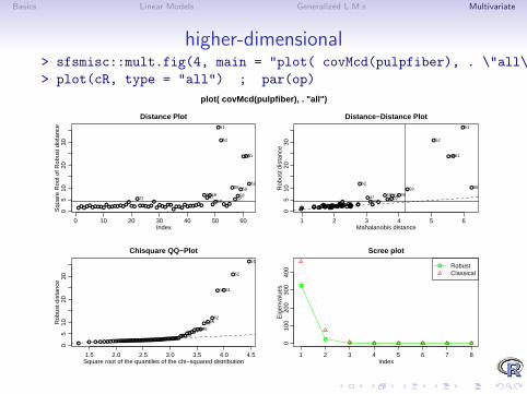
higher-dimensional> sfsmisc::mult.fig(4, main = "plot( covMcd(pulpfiber), . \"all\")")$old.p -> op> plot(cR, type = "all") ; par(op)
plot( covMcd(pulpfiber), . "all")
●●●●●●●●●●●
●●●●●●●●
●●
●
●●●●●●
●●●●
●●●
●●●●●●●●●●
●●
●
●●
●
●
●●●
●
●●
●
●●
●
0 10 20 30 40 50 60
05
1020
30
Distance Plot
Index
Squ
are
Roo
t of R
obus
t dis
tanc
e 51
52
6160
6256 59
46 48 584722 5750
● ● ●●●● ● ●●●
●● ●●● ●● ●
●●●
●
● ●●● ●●
●●●●
●●●
● ●●●● ●● ● ●●
●●
●
●●
●
●
●●●
●
●●
●
● ●
●
1 2 3 4 5 6
05
1020
30
Distance−Distance Plot
Mahalanobis distance
Rob
ust d
ista
nce
51
52
6160
625659
4648 5847 225750
● ● ● ● ●●●●●●●●●●●●●●●●●●●●●●●●●●●●●●●●●●●●●●●●●●●●●
●●●●●●
● ●●
● ●
●
●
1.5 2.0 2.5 3.0 3.5 4.0 4.5
05
1020
30
Chisquare QQ−Plot
Square root of the quantiles of the chi−squared distribution
Rob
ust d
ista
nce
505722475848465956
62
60 61
52
51
1 2 3 4 5 6 7 8
010
020
030
040
0
Index
Eig
enva
lues
● RobustClassical
●
●● ● ● ● ● ●
Scree plot

Basics Linear Models Generalized L.M.s Multivariate
Questions on Section 4 — “Multivariate Analysis” ?