Excel 2007 Tutorial - Draft · Excel 2007 Tutorial - Draft National Computational Science Institute...

Excel 2007 Tutorial - Draft

National Computational Science Institute 1

These notes will serve as a guide and reminder of several features in Excel 2007 that make the use of a spreadsheet more like an interactive thinking tool. The basic features/options to be explored are: Menus and Ribbons Naming constants or parameters Formulas Interactive controls Graphs Iteration Conditional Formatting Definitions Menus and Ribbons Note that the new Microsoft Office suite has changed from using toolbars to using ribbons. So now, when you select a menu item, a ribbon will appear with a wide array of icons to choose from. The resulting choices are fairly different from the menu items that appeared in the older versions. You may choose to always view the ribbons or to have the ribbons “pop-up” when you choose a menu. Right clicking on the menu bar displays the options shown below allowing you to choose whether to display or minimize the ribbon.

This is the Formula Bar. The text box on the left is where the names of cells are displayed, and the text box on the right is where formulas are displayed.

Names Many times it is more helpful to use a word or name to describe a constant in a spreadsheet. It may be easier to refer to a cell by a name like “Interest_Rate” or “Books” or “Percentage” or “Enrollment” rather than “$G$4” or “A7.” The use of names often makes formulas easier to understand, remember, and use.



There are two basic ways to name a cell: Using the menu: Select the cell you want to name. From then top menu, select Formulas Define Name Define Name. If you have a label “near” this cell, Excel will guess that name. If this is the name you want, just click [OK]. If you don’t have a label, or if you want a different name, type a name then click [OK]. Using the Formula Bar to Name a Cell: Select the cell you want to name. Click inside the name box. This will automatically highlight the default name of the cell. Type a name in the name box.* Hit [Enter].

* Remember: Names can only use letters, numbers, or an underscore. Use an underscore for a space.

- Deleting a name - From then top menu, select Formulas Name Manager. Select the name you want to delete and click [Delete] Note that naming a cell creates an absolute reference to that cell when it is used in a formula. Absolute referencing and relative referencing will be discussed later in the tutorial under the topic formulas.

Formulas By default, when you copy a formula into a cell, its value changes in relation to other cells. This is called relative referencing. Every formula begins with an equals sign (=). This works as a signal to the computer that you are entering a formula. Formulas look like this:

In order to get this: Type this:

= (Click on B3) / 2

= (Click on B3) * 10

= (Click on B3) + (Click on C4)

= (Click on Interest_Rate) – (Click on D3)



“B3”, “C4” and “Interest_Rate” are all names of cells in the document. You can either type the name of the cell you want to add to your formula, or you can click on it and the name will be automatically added for you. Hit [Enter] in order to calculate the formula and escape formula mode.

- Copying Formulas - What if you wanted to apply the same formula to an entire column? Should you type in the value for every cell? That would be very tedious, and thankfully it’s unnecessary. In order to fill every cell in a column with a formula, activate the cell that contains the formula you wish to copy. You will see a black dot in the lower right hand corner of this cell called the control handle. Click on the control handle and drag down and the formula will be copied into every cell beneath it.

The “IF” function A tremendous amount of the power of automatic computation is the ability to specify an “IF…Then…Else” branch scenario. If something is true, THEN set the value of the cell equal to one number, ELSE set the value of the cell equal to something else. In Excel, the IF function serves this purpose. Suppose we had a bank willing to pay 5 percent interest if our bank balance was greater than $1000, or 2 percent if it is less than or equal to $1000. In a cell, the function would look something like this: =IF(BALANCE>1000,.05,.02) This has the form: =IF(LOGICAL TEST , VALUE IF TRUE , VALUE IF FALSE) The “=” in front of the “IF” tells Excel to evaluate this expression, and that it is not just text. This can be a very powerful thinking tool, and “If” statements can be nested by making the “Value if true” or “Value if false” parts of the function another IF function.

Scroll Bars and Spinners A scroll bar is used to interactively change the value of a cell and any cells or graphs that depend on the cell controlled by a scroll bar. This allows you to see how the results in a cell, chart, or graph change as the data changes. A spinner also allows you to increase or decrease the value of a cell, but differs from a scroll bar in not having a slider control “knob”.



First, you must enable the Developer menu if it does not already appear as one of your menu choices. To enable the Developer menu click on the Microsoft Logo button then Excel Options, then make sure the Show Developer tab in the Ribbon item is checked:

The word Developer should now appear as a menu item. Select Developer Insert Form Controls and choose the scroll bar option as circled in the image. Be sure NOT to choose the scroll bar from the ActiveX controls. Your mouse will change to a thin crosshair that allows you to draw a rectangle. Drag over the area where you would like your scroll bar to be located and the scroll bar will appear.

– Modifying properties of a scroll bar –

Once you create your scroll bar, you still need to tell the scroll bar what cell it will control. To do this, right click (or [ctrl] click) on the scroll bar and select Format Control from the resulting menu:



This window will pop up → - Current value: value right now - Minimum value: the lowest setting - Maximum value: the highest setting - Incremental change: how much the value will change with one click of the arrow button - Page change: how much the value will change if you click on the scroll bar itself. - Cell link: the cell whose value will be affected by the scroll bar.

- Linking the scroll bar to a cell - In the Format Control menu, use the cell link option to tell the scroll bar which cell it is modifying. Click the button that looks like this: You will get something that looks like this:

Click on the cell you want the scroll bar to modify and this will enter the cell location in the text area, then hit [Enter] or [Return]. If you have named a cell, you can refer to the cell by its name.



- Limitations of a scroll bar -

A scroll bar will not manipulate cells containing decimals or negative numbers. This means that if you need a scroll bar to manipulate a value that is negative or a decimal the cell it controls will be a helper cell and then use that helper value in another cell to create the value you need. In this example, the actual percentage is 0.22. The value the scroll bar is modifying is 22:

So the formula to create the percent as a decimal is “= C3 / 100”. Think of it this way: S/100 is some fraction, so (S/100)*(B-A) is a fraction of the distance from the left end point A of your range (B-A) to the right end point B. If you want finer granularity, use a bigger value than 100 in both the scroll bar format control and in your corresponding formula. General formula for a scroll bar with a range of A to B: Set the range on the slider from 0 to 100, choose a cell S for the slider to control, then build a formula in a different cell: = A + (S/100) * (B-A). Note: this “linear transformation is a powerful skill and an example of both algebraic thinking and algorithmic thinking. Math teacher often finti it useful to have the students carefully think through and reflect on this control feature.

Graphs Graphs and charts help you to visualize information.

Highlight the information you would like to graph:



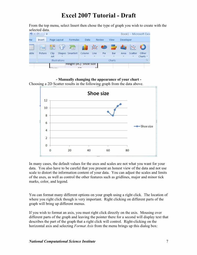
From the top menu, select Insert then chose the type of graph you wish to create with the selected data.

- Manually changing the appearance of your chart -

Choosing a 2D Scatter results in the following graph from the data above.

In many cases, the default values for the axes and scales are not what you want for your data. You also have to be careful that you present an honest view of the data and not use scale to distort the information content of your data. You can adjust the scales and limits of the axes, as well as control the other features such as gridlines, major and minor tick marks, color, and legend. You can format many different options on your graph using a right click. The location of where you right click though is very important. Right clicking on different parts of the graph will bring up different menus.

If you wish to format an axis, you must right click directly on the axis. Mousing over different parts of the graph and leaving the pointer there for a second will display text that describes the part of the graph that a right click will control. Right-clicking on the horizontal axis and selecting Format Axis from the menu brings up this dialog box:



By default the Auto radio buttons are chosen. To choose your own scales, select the fixed radio button of the option you would like to change and then type in the desired value. Minimum and Maximum:

Determine the limits of the axis

Major unit and minor unit: Determine the increments of how the axis will be divided

In order to manually change or add in axis titles click anywhere in the chart area and this will display the Chart Tools Ribbon. On the ribbon, select the layout menu and click on Axis Titles.

From the resulting drop down menu choose the title below axis option and text will appear below that axis on the graph. Click on that text to change it and type in the title accordingly. This is how the chart looked after setting the following options:

• the minimum height on the horizontal axis to 55 • the minimum shoe size on the vertical axis to 6 • the axis titles to read Height (inches) and Shoe Size • the chart title to read Shoe Size vs Height



Iteration In Excel, you sometimes want a “circular reference” which is normally not allowed. An example would be a formula for a cell that refers to itself, or two cells that refer to each other. However, by default, Excel does not allow circular reference, also known as iteration. To

enable iterative calculations, click on the Microsoft Logo Button: Select the Formula menu from the resulting pop-up window and check the enable iterative calculation check box.



Conditional Formatting Sometimes you want to use a visual cue to help your eye “spot” important data conditions. By using conditional formatting you can change a cell’s font color, pattern, or background color based on the value of the cell itself. For example, suppose you wanted to take a table of grades and make it easy to spot high and low grades. Consider the starting table → In this example, there are five test scores, and one of them is below 70, and two of them are above 90. Our goal is to make it easier to “see” this right away by coloring the cell, for instance, red to signal a caution for a low score, yellow to signal for a not so good score and green to signal good work for a high score.

Start by selecting the cells to be “conditioned” by selecting cells B2:B6. Then, from the Home tab ribbon, select Conditional Formatting and this menu will be displayed →

There are a number of options to select from. Selecting Color Scales and the first menu option produces this:



There are of course many pre-designed options to choose from or you can create your own by choosing “New Rule” from the drop down menu shown above.

- Definitions - Spreadsheet A rectangular grid for storing information

Cell Rectangular divisions in a spreadsheet. Data is entered in cells.

Column Vertical lines of cells. (Labeled by letters)

Row Horizontal lines of cells (Labeled by numbers) Scroll bar / Slider bar A tool which can change the value of a cell by regular increments

Relative Reference

Referencing a cell so that when a formula is copied from one cell to another, the name of the cell changes relative to the location of the cell the formula is copied into.

Absolute Reference

Referencing a cell so that when a formula is copied from one cell to another, the name of the cell DOES NOT change relative to the location of the cell the formula is copied into. Naming a cell creates an absolute reference.

Excel 2007 Tutorial - Draft · Excel 2007 Tutorial - Draft National Computational Science Institute...

Documents

Transcript of Excel 2007 Tutorial - Draft · Excel 2007 Tutorial - Draft National Computational Science Institute...