Exact HAM Solutions for the Viscous Rotational Flowfield

in Channels with Regressing and Injecting Sidewalls

Joseph Majdalani∗

University of Tennessee Space Institute, Tullahoma, TN 37388, USA

Hang Xu† and Zhi-Liang Lin‡ and Shi-Jun Liao§

Shanghai Jiao Tong University, Shanghai 200030, China

This paper focuses on the theoretical treatment of the laminar, incompressible, and time-dependent flow of

a viscous fluid in a porous channel with orthogonally moving walls. Assuming uniform injection or suction at

the porous walls, two cases are considered for which the opposing walls undergo either uniform or non-uniform

motions. For the first case, we follow Dauenhauer and Majdalani 1 by taking the wall expansion ratio α to be

time invariant and then proceed to reduce the Navier-Stokes equations into a fourth order ordinary differential

equation (ODE) with four boundary conditions. Using the Homotopy Analysis Method (HAM), an optimized

analytical procedure is developed that enables us to obtain highly accurate series approximations for each

of the multiple solutions associated with this problem. By exploring wide ranges of the control parameters,

our procedure allows us to identify dual or triple solutions that correspond to those reported by Zaturska,

Drazin and Banks. 2 Specifically, two new profiles are captured that are complementary to the type I solutions

explored by Dauenhauer and Majdalani. 1 In comparison to the type I motion, the so-called types II and III

profiles involve steeper flow turning streamline curvatures and internal flow recirculation. The second and

more general case that we consider allows the wall expansion ratio to vary with time. Under this assumption,

the Navier-Stokes equations are transformed into an exact nonlinear partial differential equation that is solved

analytically using the HAM procedure. In the process, both algebraic and exponential models are considered

to describe the evolution of α(t) from an initial α0 to a final state α1. In either case, we find the time-dependent

solutions to decay very rapidly to the extent of recovering the steady-state behavior associated with the use of a

constant wall expansion ratio. We then conclude that the time-dependent variation of the wall expansion ratio

plays a secondary role that may be justifiably ignored.

I. Introduction

Studies of laminar motions through porous channels continue to receive attention in the fluid and mathematical

communities due to their interesting connections with a variety of applications. These include binary gas diffusion,

filtration, ablation cooling, surface sublimation, and the modeling of air circulation in the respiratory system. Berman3

initiated the analysis of the steady laminar flow of a viscous incompressible fluid in a two-dimensional porous channel

with uniform injection or suction. With the assumption that the transverse velocity component remained independent

of the streamwise coordinate, Berman reduced the Navier-Stokes equations to a nonlinear ordinary differential equation

with appropriate boundary conditions. He then proceeded to construct an asymptotic approximation for a small

Reynolds number R using a regular perturbation scheme.

Extensions to Berman’s solution3 followed shortly thereafter. For example, Terrill4 obtained series solutions

for both small and large values of R that compared favorably with the numerical solutions to this problem. Using the

method of averages, Morduchow5 presented a solution which covered the entire injection range. Later, White, Barfield

and Goglia6 derived a power series expansion that appeared to retain its validity for arbitrary R. However, their

solution required the numerical calculation of numerous power series coefficients that could not be tied recursively.

Other studies devoted to the analysis of the symmetrically porous channel flow problem were reported by a diverse

group of investigators. To list a few, we enumerate: Sellars,7 Shrestha,8 Robinson,9 Skalak and Wang,10 Brady,11

Durlofsky and Brady,12 Zaturska, Drazin and Banks,2 Taylor,13 and Yuan.14

Following this string of investigations, at least two prominent categories of flow variations emerged, thus creating

new tracks for sustained research inquiry. The attendant motions incorporated either asymmetries in the mean flow

∗H. H. Arnold Chair of Excellence in Advanced Propulsion, Mechanical, Aerospace and Biomedical Engineering Department. Senior Member

AIAA. Fellow ASME.†Lecturer, State Key Laboratory of Ocean Engineering, School of Naval Architecture, Ocean and Civil Engineering.‡Lecturer, State Key Laboratory of Ocean Engineering, School of Naval Architecture, Ocean and Civil Engineering.§Cheung Kong Professor, State Key Laboratory of Ocean Engineering, School of Naval Architecture, Ocean and Civil Engineering.

1

American Institute of Aeronautics and Astronautics

46th AIAA/ASME/SAE/ASEE Joint Propulsion Conference & Exhibit25 - 28 July 2010, Nashville, TN

AIAA 2010-7079

Copyright © 2010 by J. Majdalani, H. Xu, Z. L. Lin and S. J. Liao. Published by the American Institute of Aeronautics and Astronautics, Inc., with permission.

configuration, or translational movement of the boundaries. The class of asymmetrical flows could be achieved, for

example, by imposing different wall suction rates, as in the case examined by Proudman15 under steady laminar

conditions and large Reynolds numbers. In the interim, the flow analog at small R was being investigated by Terrill

and Shrestha.16 Shrestha and Terrill17 also provided accurate series solutions for large wall injection using the method

of inner and outer expansions.

The problem comprising moving boundaries appears to have been initiated by Brady and Acrivos.18 These

researchers obtained an exact solution to the Navier-Stokes equations for the flow in a channel with an accelerating

surface velocity. Their work was revisited in the context of a moving porous wall by Watson et al.19 One year later,

Watson et al.20 combined asymmetry with wall movement in their analysis of the two-dimensional porous channel.

Along similar lines, Dauenhauer and Majdalani1 presented a new similarity solution for the laminar, incompressible,

and time-dependent Navier-Stokes equations in the context of a porous channel with expanding or contracting walls.

Assuming a constant (or quasi-constant) wall expansion ratio α, they reduced the Navier-Stokes equations into a self-

similar ODE that could be solved numerically. Their approach employed Runge-Kutta integration coupled with a

rapidly converging shooting technique to cover a modest range of R and wall expansion ratios. Asymptotic solutions

for the problem were later provided by Majdalani and Zhou21 for moderate-to-large R, and by Majdalani, Zhou and

Dawson22 for small R. The solution in the context of rocket propulsion is also discussed by Zhou and Majdalani.23

As for the stability of these flows, this vital topic was originally addressed by Zaturska, Drazin and Banks,2 although

several illuminating investigations have been carried out by MacGillivray and Lu,24 Lu,25 and Cox and King,26 to

name a few.

In this paper, we revisit the porous channel flow problem with regressing walls and solve it using a series approach

known as the Homotopy Analysis Method (HAM). This method was advanced by Liao27–31 as an improvement over

the Adomian decomposition framework. In this context, it was developed for the purpose of obtaining series solutions

to strongly nonlinear differential equations. Its implementation involves the introduction of an embedding parameter q

that permits converting the nonlinear governing equation into a linear equation for q = 0. As q is increased, homotopy

ensures that the original nonlinear equation is recovered in the limit of q → 1. As discussed in several articles,32–39

HAM has been shown to exhibit several distinct advantages over other asymptotic techniques. For example, HAM

provides a convenient control parameter ~ that helps to ensure series convergence.28–31 HAM can also be applied

with equal level of ease to nonlinear ODEs and PDEs. This makes it an ideal approach for handling the Dauenhauer-

Majdalani PDE considered in this study.

To set the stage, we first revisit the exact similarity equation rendered by Dauenhauer and Majdalani1 for the

porous channel flow. Given that these investigators were mainly interested in the type I injection and suction solutions

that pertained to their application, our analysis will seek to unravel not only the classical type I, but other possible

solutions that have been classified as types II and III by Zaturska, Drazin and Banks.2 To this end, an optimal HAM-

based approach will be developed with the capability of capturing multiple solutions. This will enable us to obtain

multiple solutions under suction dominated conditions that have not been discussed before. By way of verification,

our series approximations will be shown to agree substantially well with the numerically integrated solution described

by Dauenhauer and Majdalani.1

In seeking further generalization, the Dauenhauer-Majdalani model1 will be extended to the case for which the

wall expansion ratio α is no longer constant, but rather a time-dependent variable that transitions from α0 to α1. The

corresponding similarity equation is readily turned into a nonlinear partial differential equation (PDE) that can be

solved analytically. While it would be helpful to consider a case for which the channel half-height a varies from an

initial value a0 to a final a1, such a situation may be considered to be a special case of the model used here. For

example, knowing the initial and final heights, one can calculate the average expansion ratio using, for example,

a ≈ (a1 − a0)/(t1 − t0), where t1 − t0 represents the time for expansion. Then knowing a, one can calculate α0 = aa0/ν

and α1 = aa1/ν, where ν is the kinematic viscosity.

The basic equations for the channel flow problem with both constant and time-dependent wall expansion ratios

are described in Sec. II. In Sec. III, a conventional HAM approach is implemented for the purpose of capturing one

of the multiple solutions. This is followed by the presentation of an optimal HAM-based approach that can be used

to identify any number of solutions: single, dual, or triple solutions for the case of a constant wall expansion ratio.

Therein, results are described and verified through comparisons with the numerical results obtained from the use of

the Dauenhauer and Majdalani shooting approach.1 In Sec. IV, a HAM-based approach is advanced for the case of a

time-dependent wall expansion ratio. Finally, closing remarks and conclusions are given in Sec. V.

2

American Institute of Aeronautics and Astronautics

II. Formulation

A. Fundamental Equations

As shown in Fig. 1, the flow to be studied takes place in a two-dimensional rectangular channel bounded by

porous walls at y = ±a. The walls of the channel undergo either uniform or non-uniform expansion or contraction

in the transverse direction. Through the two opposing walls fluid is uniformly injected or extracted at a constant

speed vw. The governing equations describing the unsteady flow of an incompressible fluid for mass and momentum

conservation are

∂u

∂x+∂v

∂y= 0, (1)

∂u

∂t+ u

∂u

∂x+ v

∂u

∂y= −

1

ρ

∂p

∂x+ ν

(

∂2u

∂x2+∂2u

∂y2

)

, (2)

∂v

∂t+ u

∂v

∂x+ v

∂v

∂y= −

1

ρ

∂p

∂y+ ν

(

∂2v

∂x2+∂2v

∂y2

)

. (3)

x

y

0

a(t)

da/dtRegressing and injecting sidewall

Figure 1. Coordinate system and characteristic streamlines.

These are subject to the following

boundary conditions:

u = 0, v = −vw; y = a(t), (4)

∂u

∂y= 0, v = 0; y = 0, (5)

u = 0, v = 0; x = 0, (6)

where Cartesian coordinates (x, y) that are

fixed in space are taken, with the x-axis

extending along the length of the channel

and the y-axis in the wall-normal direction.

Here u and v denote the velocity components

along x- and y-axes, and ρ, p, ν, t, and

vw correspond to the dimensional density,

pressure, kinematic viscosity, time, and

(crossflow) injection velocity at the wall.

Note that Eqs. (4-6) are written in the upper half-domain (y ≥ 0), thus taking into account symmetry with respect

to the midsection plane while assuming an odd function for the wall normal velocity v and an even function for the

axial velocity u.

Using ψ to denote a stream function such that u = ∂ψ/∂y and v = −∂ψ/∂x, the continuity equation is automatically

satisfied and the vorticity transport equation is readily obtained by taking the curl of the momentum equation. One

gets

∂ζ

∂t+ u

∂ζ

∂x+ v

∂ζ

∂y= ν

(

∂2ζ

∂x2+∂2ζ

∂y2

)

, (7)

where

ζ =∂v

∂x−∂u

∂y= −∇2ψ. (8)

Substituting the dual transformations1

ψ = (νx/a)F(η, t), η = y/a (9)

into the vorticity transportation equation gives

[Fηηη + FFηη + Fη(2α − Fη) + α ηFηη − (a2/ν)Fηt]η = 0, (10)

3

American Institute of Aeronautics and Astronautics

which is subject to the four classical boundary conditions

η = 0 : F = 0, Fηη = 0

η = 1 : F = R, Fη = 0.(11)

Equation (10) describes the unsteady flow of an incompressible fluid in a porous channel. It is presented by White40

as one of the new exact Navier-Stokes solutions for channel flows.1 Here

α = aa/ν (12)

is the wall expansion ratio in which a and a represent the half-height of the channel and its expansion speed; as before,

ν is the kinematic viscosity and so R = vwa/ν = Aα defines the crossflow Reynolds number, with A being the injection

coefficient. Note that according to our sign convention, a positive R refers to injection conditions. More detail is given

by Dauenhauer and Majdalani1 where these steps are systematically developed.

B. Uniform Wall Regression

When the wall expansion ratio α is constant in time, the function F becomes dependent on η and α instead of (η, t).

One can put Fηt = 0 and write

α = aa/ν = a0a0/ν (13)

where a0 and a0 are the initial channel height and expansion rate, respectively. Integrating Eq. (13) with respect to t

yields

a/a0 = (1 + 2ναta−20 )1/2. (14)

Moreover, given a constant injection coefficient A, one can put

a/a0 = vw(t)/vw(0) = (1 + 2ναta−20 )−1/2. (15)

As shown by Dauenhauer and Majdalani,1 an exact self-similarity equation emerges for Berman’s main

characteristic function F. After some algebra, one retrieves

Fηηηη + FFηηη + Fηη(3α − Fη) + α ηFηηη = 0, (16)

with

η = 0 : F = 0, Fηη = 0; η = 1 : F = R, Fη = 0, (17)

where F denotes a sole function of η. For more detail on the mathematical foundations of Eqs. (16) and (17), the

reader is referred to Dauenhauer and Majdalani.1

C. Non-Uniform Wall Regression

Another practical setting corresponds to the case for which the wall expansion ratio α is not restricted to a constant,

but is rather permitted to vary as a function of t, namely, from α0 to α1. Letting

β(t) =a2

ν, (18)

it follows that

α(t) = aa/ν = 12βt(t). (19)

Then taking into account Eq. (12), we can put

α0(t) = α(0) = a0a0/ν =12βt(0). (20)

If we now consider the hypothetical case for which the injection coefficient A is inversely proportional to α(t), Eq.

(10) can be reduced to

Fηηηη + α(t)(

ηFηηη + 3Fηη

)

+ FFηηη − FηFηη − β(t)Fηηt = 0, (21)

where F = F(η, t). This PDE is subject to the same fundamental boundary conditions delineated in Eq. (17). Its

formulation constitutes another exact reduction of the Navier-Stokes equations that will be discussed in Sec. IV.

4

American Institute of Aeronautics and Astronautics

III. Constant Regression Ratio

A. Conventional HAM Approach

In this section, we provide an accurate analytical approximation to Eq. (16). With the help of the Homotopy

Analysis Method, the explicit approximations for F(η) can be specified as

F(η) =

M∑

m=0

φm(η) =

M∑

m=0

4m+4∑

i=0

λmi am

i ηi, (22)

where φm(η) is the mth-order homotopy-derivative, defined in the Appendix by Eq. (115), and the coefficients ami

are

given by

am1 = χmλ

m−11 am−1

1 +C1m, (23)

am3 = χmλ

m−13 am−1

3 +C3m, (24)

ami = λ

m−1i am−1

i +~(em−1

i−4+ 3αcm−1

i−4+ χi−3dm−1

i−5+ Υm

i−4+ Ωm

i−4)

i(i − 1)(i − 2)(i − 3), (25)

for 3 < i ≤ 4m + 3, in which

bmi = (i + 1)λm

i+1ami+1, (26)

cmi = (i + 2)(i + 1)λm

i+2ami+2, (27)

dmi = (i + 3)(i + 2)(i + 1)λm

i+3ami+3, (28)

emi = (i + 4)(i + 3)(i + 2)(i + 1)λm

i+4ami+4, (29)

Υmi =

m−1∑

k=0

max4k+4, i∑

r=max0, i−4m+4k

λkrak

rbm−k−1i−r , (30)

Ωmi =

m−1∑

k=0

max4k+4, i∑

r=max0, i−4m+4k

bkrcm−k−1

i−r , (31)

Cm0 = Cm

2 = 0, (32)

Cm3 =~

2

4m+4∑

i=0

em−1i−4+ 3αcm−1

i−4+ χi−3dm−1

i−5+ Υm

i−4+ Ωm

i−4

i(i − 1)(i − 2)(i − 3)

−~

2

4m+4∑

i=0

em−1i−3+ 3αcm−1

i−3+ χi−2dm−1

i−4+ Υm

i−3+ Ωm

i−3

i(i − 1)(i − 2), (33)

Cm1 = −

4m+4∑

i=0

em−1i−4+ 3αcm−1

i−4+ χi−3dm−1

i−5+ Υm

i−4+ Ωm

i−4

i(i − 1)(i − 2)(i − 3)− Cm

3 , (34)

χm =

0,m = 1,

1,m > 1(35)

and

λmi =

1, 1 ≤ i ≤ 4m + 3,

0, i < 1 or i > 4m + 3.(36)

Using the initial guess function given by

φ0(η, t) = 12R η(3 − η2), (37)

5

American Institute of Aeronautics and Astronautics

the first four coefficients are found to be

a01 =

32R, a0

2= 0, a0

3= − 1

2R, a0

4= 0. (38)

At this juncture, the explicit HAM series coefficients are fully determined. Other flow variables such as the velocity,

pressure and vorticity may be readily evaluated from their basic definitions. For example, the vorticity ζ may be

retrieved from Eq. (8) viz.

ζ = −∇2ψ =∂v

∂x−∂u

∂y= −νxa−3Fηη. (39)

Other variables are omitted here for the sake of brevity. It may be worth remarking that the convergence of the HAM

approximations is guaranteed when the linear operator L, the initial guess φ0(η), and the values of the convergence-

control parameter ~ are obtained in accordance with pre-established rules.28,29 Usually, L and φ0(η) are constructed

based on the solution expression consistently with the nonlinear behavior associated with the problem at hand. In this

first section, we use ~ = −1. In a later section, we confirm that series convergence is guaranteed for ~ ∈ [− 32,− 2

3],

albeit not limited to this range exclusively.

In order to test the accuracy of our traditional HAM series approximations with ~ = −1, we compare in Figs. 2a and

2b the HAM solution for the axial velocity, given by F′(η)/R, to the numerical results of Eq. (16). The corresponding

curves are evaluated for R = ±5 and values of α ranging from −20 to 5. Clearly, a uniformly consistent agreement

with numerics is realized owing, in large part, to the ability of the HAM approximation to capture the true, nonlinear

behavior of the solution in the limit of an infinite series.

For the suction driven channel with no wall motion, Zaturska, Drazin and Banks2 have shown that one symmetric

solution exists for R ∈ [−12.165, 0] and three symmetric solutions emerge when R ∈ [−∞,−12.165]. In much the

same way, the search for multiple solutions will have to be influenced by both α and R, thus requiring a separate

mathematical treatment, as first explained by Dauenhauer and Majdalani.1 This treatment will be carried out in the

next section. In the interim, the numerical technique used by Dauenhauer and Majdalani1 will be used to study the

emergence of solution multiplicity in suitable ranges of α and R. This is evident in Fig. 3 where one particular

case is considered (e.g. α = 1 and R = −20) for which three solution branches are seen to co-exist. Using the

conventional HAM approach, only type I can be predicted, although three types can be projected numerically. This

apparent deficiency prompts us to modify the conventional HAM approach to the extent of granting it more generality.

As we describe in the next section, the extension will enable us to capture, using analytical series approximations, the

η

F’

(η)/

R

­1 ­0.5 0 0.5 1­1

­0.5

0

0.5

1

1.5

2

2.5

3

α = ­20, ­10, ­5, 0, 1, 2, 2.5

a) R = −5

η

F’

(η)/

R

­1 ­0.5 0 0.5 10

0.5

1

1.5

2

α = ­20, ­10, ­5, 0, 5

b) R = 5

Figure 2. Comparison between HAM-Pade approximations (circles) and numerical results (solid lines) over a range of α using a) R = −5

and b) R = 5.

6

American Institute of Aeronautics and Astronautics

three types of mean flow motions that are discussed by Zaturska, Drazin and Banks2 in the case of a non-expanding

wall.

B. Optimal Strategy for Multiple Solutions

η

F’

(η)/

R

0 0.1 0.2 0.3 0.4 0.5 0.6 0.7 0.8 0.9 1­4

­3

­2

­1

0

1

2

3

4

5

Type III

Type II

Type I

α = 1, R = ­20

numeric

Figure 3. Three types of solutions for F′(η)/R at α = 1 and R = −20.

In what follows, we describe the mathematical steps

needed to mold the Homotopy Analysis Method to the

porous channel flow problem with a constant expansion

ratio α. We thus consider the steady PDE given by Eq.

(16) and focus on its multiple solutions.

Note that there exist dual or even triple solutions for

some values of α and R. In general, multiple solutions

can be elusive even by numerical methods. Here,

we provide an analytical framework that enables us to

capture these multiple solutions. First, we introduce the

transformation

F(η) = R S (η), (40)

and so, the original equation becomes

S ′′′′ + α(

ηS ′′′ + 3S ′′)

+ R(S S ′′′ − S ′S ′′) = 0, (41)

subject to the boundary conditions

S (0) = 0, S ′′(0) = 0, S (1) = 1, S ′(1) = 0, (42)

where the prime denotes a derivative with respect to η. To help identify the multiple solutions that accompany different

α and R, we define F′(0) = R γ, where

γ = S ′(0). (43)

Our strategy is guided by the shooting method described earlier.1 Instead of using the original boundary conditions

(42), we first apply HAM to secure analytical approximations for Eq. (41) using an initial value for S ′(0) at the lower

end of the domain. We hence take

S (0) = 0, S ′(0) = γ, S ′′(0) = 0, S (1) = 1, (44)

where γ is not known initially. At the conclusion of the analysis, γ may be determined from the actual boundary

condition that must be observed at the upper end of the domain, specifically

S ′(1) = 0. (45)

At this juncture, the form of the analytical solutions to Eqs. (41) and (44) must be posited in terms of suitable

functions. Given that Eq. (41) is defined over a finite domain η ∈ [0, 1], it is proper to express S (η) in a power series

of η. Besides, using Eq. (41) and the boundary conditions S (0) = 0 and S ηη(0) = 0, it can be shown that

d2kS

dη2k

∣

∣

∣

∣

∣

∣

η=0

= 0, when k = 1, 2, 3, · · · (46)

Thus, S (η) may be expressed as

S (η) =

+∞∑

m=0

Bm η2m+1, (47)

where the undetermined coefficient Bm is dependent on α. Equation (47) defines what is often referred to as the solution

expression for S (η). According to the homotopy-based approach, one needs to introduce an initial guess function of

the form prescribed by Eq. (47) that still satisfies the problem’s boundary conditions. For this reason, we choose, for

the case of a constant wall expansion ratio, the following odd polynomial:

S 0(η) = A0 η + A1 η3 + A2 η

5. (48)

7

American Institute of Aeronautics and Astronautics

This initial guess function may be readily made to satisfy the conditions given by Eqs. (44) and (45). The result is

A0 = γ, A1 =5

2− 2 γ, A2 = γ −

3

2, (49)

whence

S 0(η) = γ η +

(

5

2− 2 γ

)

η3 +

(

γ −3

2

)

η5. (50)

As with perturbation and traditional non-perturbation methods, HAM transforms a nonlinear problem into an

infinite number of linear sub-problems. Additionally, HAM provides greater freedom in selecting different base

functions that serve to approximate solutions more efficiently. Equally importantly, perhaps, HAM provides the means

to ensure the convergence of ensuing series solutions. This is accomplished through the use of the convergence-control

parameter ~. By way of illustration, we note that, even for the nonlinear ODE, Eq. (41), it is not convenient to employ

its entire linear part L = S ′′′′ + α (η S ′′′ + 3S ′′) as the linear operator. Otherwise, the L = 0 solution would contain

the error function Erf(η); it would then become exceedingly difficult to retrieve higher-order approximations. This

obstacle can be overcome by selecting an auxiliary operator of equal order, in this case, of fourth order, such as,

LΦ =d4Φ

dη4. (51)

This operator has the property

L(C0 +C1η + C2η2 +C3η

3) = 0, (52)

where (C0,C1,C2,C3) are integral constants. This linear approximation is sufficient to satisfy the rule of solution

expression, Eq. (47). It should be noted that, the solution for S (η), where η ∈ [0, 1], represents a mapping operation

of S : [0, 1] 7−→ (−∞,+∞). Instead of solving Eq. (41) directly, we undergo continuous mapping according to

Φ(η; q) : [0, 1] × [0, 1] 7−→ (−∞,+∞) (53)

where

Φ(η; 0) = S 0(η), Φ(η; 1) = S (η). (54)

The mapping operation follows from the zeroth-order deformation equation

(1 − q)L[Φ(η; q) − S 0(η)] = q ~ N[Φ(η; q)], (55)

which is subject to

Φ(0; q) = 0,∂Φ(η; q)

∂η

∣

∣

∣

∣

∣

η=0

= γ,∂2Φ(η; q)

∂η2

∣

∣

∣

∣

∣

∣

η=0

= 0, Φ(1; q) = 1. (56)

On the one hand, q ∈ [0, 1] denotes the embedment parameter mentioned before, while ~ alludes to the auxiliary

parameter known as the convergence-control parameter.27 On the other hand,L andN refer to the linear and nonlinear

operators based on Eqs. (51) and (41), respectively. The latter is defined by

N[Φ(η; q)] =∂4Φ

∂η4+ α

(

η∂3Φ

∂η3+ 3

∂2Φ

∂η2

)

+ R

(

Φ∂3Φ

∂η3−∂Φ

∂η

∂2Φ

∂η2

)

. (57)

To make further headway, one may evaluate Eq. (55) at both ends of its limiting expressions to deduce

q = 0 : L[Φ(η; 0) − S 0(η)] = 0,

q = 1 : N[Φ(η; 1)] = 0; ∀~ , 0.(58)

In the above, the initial guess S 0(η), defined by Eq. (50), satisfies the boundary conditions in Eq. (44). Hence

as we track the evolution of q across the range [0,1], the solution of the zeroth-order deformation equation will

8

American Institute of Aeronautics and Astronautics

vary continuously from the initial approximation S 0(η) to the target function S (η) that will exactly satisfy Eq. (44).

ExpandingΦ(η; q) in the Maclaurin series form with respect to q, we have

Φ(η; q) = S 0(η) +

+∞∑

m=1

S m(η) qm, (59)

where

S m(η) =1

m!

∂mΦ(η; q)

∂qm

∣

∣

∣

∣

∣

q=0

. (60)

Here, the relationship Φ(η; 0) = S 0(η) is used. It should be emphasized that the zeroth-order deformation equation

contains the convergence-control parameter ~, which is used to guarantee the convergence of the final series solution.

In principle, ~ is chosen so that the above series remains convergent at q = 1 over the entire domain, η ∈ [0, 1]. Then,

using the relationship Φ(η; 1) = S (η), we obtain the homotopy-series solution

S (η) = S 0(η) +

+∞∑

m=1

S m(η), (61)

where S m(η) is unknown. Its governing equation and related boundary conditions have to be carefully established. To

this end, we introduce the vector~S m = S 0(η), S 1(η), S 2(η), · · · , S m(η). (62)

Differentiating the zeroth-order deformation equation and the boundary conditions m times with respect to q, dividing

by m!, and then setting q = 0, we obtain the mth-order deformation equation

L[S m(η) − χmS m−1(η)] = ~ δm[S m−1(η)]. (63)

Equation (63) is subject to

η = 0 : S m = 0, S ′m = 0, S ′′m = 0; η = 1 : S m = 0, (64)

where

χm =

0, m ≤ 1,

1, m > 1,(65)

and the right-hand-side function δm is given by

δm[S m−1(η)] = S ′′′′m−1 + α (3S ′′m−1 + ηS ′′′m−1) + R

m−1∑

n=0

(S nS ′′′m−1−n + S ′nS ′′m−1−n). (66)

According to Eq. (51), it is straightforward to retrieve a particular solution S ∗m(η) of Eq. (63) by integrating the

right-hand-side term four times with respect to η, viz.

S ∗m(η) = χm S m−1(η) + ~

∫ ∫ ∫ ∫

δm[S m−1(η)] dη dη dη dη. (67)

The ensuing quad-fold integration yields

S m(η) = S ∗m(η) +Cm,0 +Cm,1 η +Cm,2 η2 +Cm,3 η

3 (m ≥ 1), (68)

where the integral constants

Cm,0 = Cm,2 = 0, Cm,1 = −dS ∗m

dη

∣

∣

∣

∣

∣

η=0

, and Cm,3 = −Cm,1 − S ∗m(1) (69)

are secured from the boundary conditions in Eq. (64). The Mth-order approximation of S (η) may hence be written as

S (η) ≈ S 0(η) +

M∑

k=1

S k(η). (70)

9

American Institute of Aeronautics and Astronautics

Note that the above expression incorporates the unknown parameter γ.

The next step is to determine the value of γ that will permit the solution to satisfy the boundary condition, Eq.

(45), at the upper end of the domain, namely, S ′(1) = 0. Substituting the Mth-order approximation, Eq. (70), into Eq.

(45) gives

ΓM(γ, ~) = S ′0(1) +

M∑

n=1

S ′n(1) = 0, (71)

where ΓM represents the expanded form of the constrained boundary condition. Using an Mth-order approximation,

we have

S M(η) =

3M+2∑

n=0

AM,n(α, γ, ~) η2n+1 (72)

and so

ΓM(γ, ~) =

M+1∑

n=0

BM,n(α, ~) γn = 0, (73)

where AM,n(α, γ, ~) and BM,n(α, ~) are coefficients of the power series of η. Note that, as long as ~ is given, the solutions

of Eq. (71) may be readily obtained.

In our quest for an optimal value of ~, we use a technique that has been shown to produce a fast converging

HAM approximation. In principle, the technique seeks to mimimize the exact square residual error of Eq. (41) at the

mth-order. This quantity is given by

Em(γ, ~) =

∫ 1

0

N

m∑

n=0

S n(η)

2

dη. (74)

In practice, however, the evaluation of Em(γ, ~) tends to be time-consuming. A simpler alternative consists of

calculating the averaged square residual error. In this vein, one may seek to minimize the zeroth order discretization

of Eq. (74):

Em(γ, ~) =1

(M + 1)

M∑

k=0

N

m∑

n=0

S n(ηk)

2

, (75)

where

ηk = k ∆η =k

M, k = 0, 1, 2, 3, · · · , M. (76)

Hereafter, a value of M = 40 will be used with the purpose of optimization. For traditional problems in which Em is

only dependent on ~, it is relatively straightforward to seek an optimal value ~∗ for which Em is minimized. However,

for the problem under consideration, the residual error is exacerbated by its dependence on both ~ and γ. In fact, both

Em(γ, ~) and ΓM(γ, ~) contain the two unknowns: γ and ~. So while the optimal convergence-control parameter ~∗ can

still be determined from the minimum of Em(γ, ~), it must be additionally subjected to the algebraic Eq. (71) needed

to secure the boundary value constant γ. For this doubly coupled optimization problem, we let (~∗, γ∗) denote the

solution of Eq. (71), which corresponds to the minimum of the square residual error. Mathematically, it holds that

(~∗, γ∗) = min Em(γ, ~), Γm(γ, ~) = 0 . (77)

For the sake of computational efficiency, the exact square residual error may be replaced by the averaged square

residual error defined by Eq. (75). To identify the optimal approximation in a region a ≤ γ ≤ b, we take

(~∗, γ∗) = min Em(γ, ~), Γm(γ, ~) = 0, a ≤ γ ≤ b . (78)

Such an operation may be relegated to symbolic programming with a dedicated ‘Minimize’ command.

Before leaving this section, it may be helpful to remark that Eq. (63) represents a linear ODE that is relatively

simple to solve. This behavior is contrary to that of Eq. (41), the original nonlinear ODE for uniform wall expansion

with α = constant. Using homotopy, the Dauenhauer-Majdalani ODE is transferable into an infinite number of linear

ODEs that can be solved directly. The ensuing transformations are made possible by the flexibility of the HAM

procedure in identifying a simple auxiliary linear operator through which the solution of the high-order deformation

equation can be readily obtained. Meanwhile, the convergence-control parameter ~ may be optimized to the extent of

accelerating or ensuring the convergence of the series approximations.28–31,41 These particular characteristics represent

some of the key features that distinguish HAM from other analytical methods.

10

American Institute of Aeronautics and Astronautics

C. Multiple Solutions

For constant α, Dauenhauer and Majdalani1 obtained an exact ODE and provided the steps that can lead to a

numerical solution using a fast-converging shooting method coupled with Runge-Kutta integration. They illustrated

their results by providing numerical solutions over a modest range of α and R that are aligned with the type I family

of solutions classified by Zaturska, Drazin and Banks.2 However, solutions of type II and III for the suction case,

particularly those leading to internal flow steepening and recirculation, were alluded to but not considered in their

article. Later studies by Majdalani and Zhou,21 Majdalani, Zhou and Dawson,22 and Zhou and Majdalani23 provided

closed-form explicit approximations over some limited ranges of suction and injection.

To illustrate how the general HAM approach may be applied, we first consider a special case of α = 4 and R = −10.

We can sequentially solve up to the mth-order deformation equations, i.e., Eqs. (63) and (64), for m = 1, 2, 3, · · · . We

hence retrieve

S 1(η) = ~

(

γ2

77+

3173γ

6930−

325

924

)

η3 − ~

(

3γ

5−

1

2

)

η5

+ ~

(

2γ2

21−γ

7+

1

28

)

η7 − ~

(

10γ2

63−

55γ

126+

25

84

)

η9

+ ~

(

5γ2

99−

5γ

33+

5

44

)

η11, (79)

S 2(η) = S 1(η) + ~2

(

63355γ3

6432426−

15323311γ2

192972780+

159557617γ

643242600−

396889

2450448

)

η3 + · · · . (80)

At the mth-order of approximation, S m(η) contains the unknown convergence-control parameter ~ and the unknown

variable γ that satisfies the right-hand-side boundary condition connected with Eq. (71). At the first and second-order

approximations, Eq. (71) yields

Γ1 = ~

(

41

154−

421γ

1155−

116γ2

693

)

= 0, (81)

and

Γ2 = ~

(

41

77−

842γ

1155−

232γ2

693

)

+ ~2

(

3215

37128−

24693629γ

107207100+

773027γ2

6432426−

2033γ3

153153

)

= 0, (82)

γ

Γ1

0

­3 ­2 ­1 0 1 2 3

­4

­3

­2

­1

0

1

2

3

4

γ2nd branch γ

1st branch

Figure 4. Curves of Γm(γ, ~) using a 10th-order HAM approximation

(m = 10) in case of α = 4 and R = −10. Solid line: ~ = −1; dashed line:

~ = − 32 ; dash-dotted line: ~ = − 2

3 .

respectively, up to Γm. Thus, the algebraic equation

Γm(γ, ~) = 0 contains not only the unknown variable

γ but also the unknown convergence-control parameter

~. Each zero γ∗ of Γm(γ∗, ~) = 0 will hence signal the

presence of a distinct solution. After determining the

number of zeroes, a proper choice of ~ can be sought

for each γ∗. It can thus be seen that the convergence-

control parameter ~ has no physical meaning besides

granting us the freedom to calibrate its value to the extent

of optimizing the solution. For example, in case of the

10th-order approximation for α = 4 and R = −10, the

curves of Γ10(γ, ~) for ~ = − 32,−1 and − 2

3are computed

and illustrated in Fig. 4. It is interesting that, although

Γ10(γ, ~) curves are sensitive to the value taken by ~, the

zeroes of the algebraic equation Γ10(γ, ~) = 0 when ~ ∈

[− 32,− 2

3] remain close. They actually become virtually

indiscernible as m is increased. The zeroes appear to be

only weakly sensitive to ~ despite the existence of two

zeroes in the regions γ ∈ (−2,−1) and γ ∈ (0, 1). Each

of these zeroes corresponds to a distinct solution.

At the given order of approximation m, the optimal convergence-control parameter ~∗ may be determined for the

positive solution of γ ∈ (0, 1) by minimizing the averaged square residual error, specifically

(~∗, γ∗) = min Em(γ, ~), Γm(γ, ~) = 0, γ > 0 . (83)

11

American Institute of Aeronautics and Astronautics

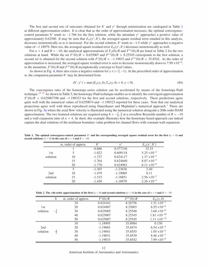
The first and second sets of outcomes obtained for ~∗ and γ∗ through minimization are catalogued in Table 1

at different approximation orders. It is clear that as the order of approximation increases, the optimal convergence-

control parameter ~∗ tends to −1.766 for the first solution, while the attendant γ∗ approaches a positive value of

approximately 0.62500. It may be seen that Em(γ∗, ~∗), the averaged square residual error entailed in this analysis,

decreases monotonically as m is increased. For the second solution, ~∗ tends to −1.5 while γ∗ approaches a negative

value of −1.18979. Here too, the averaged square residual error Em(γ∗, ~∗) decreases monotonically as well.

For α = 4 and R = −10, the analytical approximations of Fη(0)/R and F′′′(0)/R are listed in Table 2 for the two

solutions at hand. While the set F′(0)/R ≈ 0.625007 and F′′′(0)/R ≈ 8.25545 corresponds to the first solution, a

second set is obtained for the second solution with F′(0)/R ≈ −1.19033 and F′′′(0)/R ≈ 35.8542. As the order of

approximation is increased, the averaged square residual error is seen to decrease monotonically down to 7.99 ×10−8;

in the meantime, F′(0)/R and F′′′(0)/R asymptotically converge to fixed values.

As shown in Fig. 4, there also exists a negative solution for γ ∈ (−2,−1). At the prescribed order of approximation

m, the companion parameter ~∗ may be determined from

(~∗, γ∗) = min Em(γ, ~), Γm(γ, ~) = 0, γ < 0 . (84)

The convergence ratio of the homotopy-series solution can be accelerated by means of the homotopy-Pade

technique.27–31 As shown in Table 3, the homotopy-Pade technique enables us to identify the convergent approximation

F′(0)/R ≈ 0.625007396 and −1.190323 for the first and second solutions, respectively. These predictions agree

quite well with the numerical values of 0.6250074 and −1.190323 reported for these cases. Note that our analytical

projections agree well with those reproduced using Dauenhauer and Majdalani’s numerical approach.1 These are

shown in Fig. 5a where the axial flow velocity is illustrated using the numerical solution alongside a 20th-order HAM

approximation. The two featured solutions are acquired using ~ = − 74, 3

2at a crossflow Reynolds number of R = −10

and a wall expansion ratio of α = 4. In short, this example illustrates how the homotopy-based approach can indeed

capture the dual solutions of the nonlinear boundary-value problem for channel flows with constant wall expansion.

Table 1. The optimal convergence-control parameter ~∗ and the corresponding averaged square residual error for the first (γ > 0) and

second solutions (γ < 0) in the case of α = 4 and R = −10

m, order of approx. ~∗ γ∗ Em(γ∗, ~∗)

1 -0.886 0.577336 32.33

1st 5 -1.022 0.609118 5.25 ×10−2

solution 10 -1.727 0.624117 1.37 ×10−3

15 -1.764 0.624840 8.07 ×10−5

20 -1.770 0.624963 6.11 ×10−6

5 -1.303 -1.23636 2.40

2nd 10 -1.479 -1.19069 0.11

solution 15 -1.515 -1.18851 2.56 ×10−2

20 -1.458 -1.18979 2.26 ×10−4

Table 2. The mth-order approximation of the first (γ > 0) and second solutions (γ < 0) in the case of α = 4 and R = −10

~ m, order of approx. F′(0)/R F′′′(0)/R Em(γ, ~)

10 0.624161 8.26756 1.51 ×10−3

1st 20 0.624967 8.25603 6.55 ×10−6

solution - 74

30 0.625005 8.25548 3.68 ×10−8

40 0.625007 8.25545 1.81 ×10−10

50 0.625007 8.25545 1.11 ×10−12

10 -1.18995 35.8984 0.150

2nd 20 -1.19003 35.8474 6.54 ×10−4

solution - 32

30 -1.19041 35.8555 1.05 ×10−5

40 -1.19031 35.8539 8.46 ×10−7

50 -1.19033 35.8542 7.99 ×10−8

12

American Institute of Aeronautics and Astronautics

Table 3. The [m,m] homotopy-Pade approximation of the first (γ > 0) and second solutions (γ < 0) in the case of α = 4 and R = −10

m 1st solution 2nd solution

F′(0)/R F′′′(0)/R F′(0)/R F′′′(0)/R

4 0.624478732 8.265444222 -1.219891 36.01091

8 0.625005336 8.255477422 -1.178465 35.17878

12 0.625007412 8.255446248 -1.190349 35.85462

16 0.625007395 8.255446127 -1.190319 35.85409

18 0.625007396 8.255446127 -1.190319 35.85411

20 0.625007396 8.255446125 -1.190323 35.85415

22 0.625007396 8.255446124 -1.190323 35.85416

24 0.625007396 8.255446124 -1.190323 35.85416

η

F’

(η)/

R

­1 ­0.5 0 0.5 1­2

­1.5

­1

­0.5

0

0.5

1

1.5

2

2.5

3

α = 4, R = ­10Lines: HAM analyticSymbols: numeric

a) α = 4, R = −10

η

F’

(η)/

R

­1 ­0.5 0 0.5 1­3

­2

­1

0

1

2

3

α = 1.5, R = ­11Lines: HAM analyticSymbols: numeric

b) α = 32, R = −11

Figure 5. Comparison of numerical solutions with a) the 20th-order HAM approximation for F′(η)/R in case of α = 4 and R = −10.

Symbols: numerical results; dashed line: first solution with ~ = − 74

; solid line: second solution with ~ = − 32

; and b) the 30th-order HAM

approximation of F′(η)/R in case of α = 32

and R = −11. Symbols: numerical results; solid line: first solution with ~ = − 53

; dashed line:

second solution with ~ = − 53

; dash-dotted line: third solution with ~ = − 34

.

The present approach is capable of capturing triple roots when three branches of solution arise. A concrete example

consists of the case of α = 1.5 and R = −11. The corresponding curves of Γ10(γ, ~) at the 10th-order of approximation

are given in Fig. 6 using ~ = −1,− 32

and − 23. This graph clearly shows that two values of γ emerge near −1 and 0.

Besides, it appears that a third solution exists in the region of γ > 1. In the case of α = 1.5 and R = −11, Eq. (71)

produces three solutions near −1, 0 and γ > 1. In seeking an optimal convergence-control parameter, we carefully

bracket our searches within the following intervals:

(A) : min Em(γ, ~), Γm(γ, ~) = 0, −2 < γ ≤ −0.5 , (85)

(B) : min Em(γ, ~), Γm(γ, ~) = 0, −0.5 < γ ≤ 0.5 , (86)

(C) : min Em(γ, ~), Γm(γ, ~) = 0, 0.5 < γ ≤ 4 . (87)

Forthwith, the results of our analysis are posted in Table 4. We find ~∗ to be approximately − 53

for the first and

second solutions, and − 45

for the third. The HAM approximations of F′(0)/R and F′′′(0)/R associated with these

three solutions are listed in Table 5. Using the homotopy-Pade technique, we obtain F′(0)/R = −1.0237712 and

0.169352 for the first and second solutions, respectively. These values agree very well with the numerical predictions

of F′(0)/R = −1.023771 and 0.1693532 for these two branches. In contrast, we find the third solution to be more

13

American Institute of Aeronautics and Astronautics

Table 4. The optimal convergence-control parameter ~∗ and the corresponding averaged square residual error in the case of α = 1.5 and

R = −11 for three solutions of γ∗

m, order of approx. ~∗ γ∗ Em(γ∗, ~∗)

1st 4 -1.235 -0.98273 11.9

solution 8 -1.604 -1.02008 0.153

12 -1.561 -1.02275 2.37 ×10−2

16 -1.654 -1.02356 2.49 ×10−4

20 -1.625 -1.02371 1.16 ×10−4

2nd 6 -1.661 0.21276 24.6

solution 8 -1.701 0.17635 2.18

12 -1.441 0.16688 2.40 ×10−2

16 -1.146 0.16717 1.69 ×10−2

20 -1.681 0.16945 5.95 ×10−4

3rd 20 -0.951 2.75398 17.3

solution 24 -0.859 2.75736 12.2

26 -0.940 2.75098 2.70

28 -0.881 2.75936 1.09

30 -0.875 2.76689 0.37

γ

Γ10

­4 ­3 ­2 ­1 0 1 2 3 4

­4

­2

0

2

4

γ1st solution

γ3rd solutionγ

2nd solution

Figure 6. Curves of Γm(γ, ~) using a 10th-order HAM approximation

(m = 10) in case of α = 1.5 and R = −11. Solid line: ~ = −1; dashed

line: ~ = − 32

; dash-dotted line: ~ = − 23

.

ν x /a

η

0 5 10 15 200

0.2

0.4

0.6

0.8

1α = 1.5, R = ­11

Figure 7. Streamline patterns of three types of analytical solutions in

case of α = 32

and R = −11. Solid line: type I solution with F′(0)/R =2.76111; dashed line: type II solution with F′(0)/R = 0.1693532;

dash-dotted line: type III solution with F′(0)/R = −1.023771190.

difficult to retrieve. This may be attributed to its averaged square residual error remaining 5.68× 103 at the 10th-order

approximation and slowly decreasing to 1.08 × 10−3 at the 60th order (see Table 6). Everywhere, the three analytical

approximations of F′(η)/R appear to be in excellent agreement with the numerical predictions shown in Fig. 5b. This

uniformly consistent agreement with numerics is realized owing, in large part, to the ability of the HAM approximation

to capture the true, nonlinear behavior of the solution in the limit of an infinite series.

Generally speaking, the numerical identification of all possible solutions associated with nonlinear boundary-value

problems can require significant effort. For the suction driven channel flow with no wall motion, Zaturska, Drazin and

Banks2 have shown that one symmetric solution exists for R ∈ [−12.165, 0] and three symmetric solutions emerge

when R ∈ [−∞,−12.165]. In the present work, the same types of solutions are captured. Using HAM, dual solutions

are returned, for example, in the case of α = 4 and R = −10, while three distinct solutions are retrieved in the

14

American Institute of Aeronautics and Astronautics

Table 5. The mth-order approximation of the three solutions in the case of α = 32 and R = −11

~ m, order of approx. F′(0)/R F′′′(0)/R Em(γ, ~)

10 -1.022322 24.27070 0.468

1st 20 -1.023716 24.28564 1.52 ×10−4

solution - 53

30 -1.023769 24.28628 1.60 ×10−7

40 -1.023771 24.28631 5.01 ×10−10

50 -1.023771 24.28631 1.72 ×10−12

10 0.166208 10.2842 0.67

2nd 20 0.169384 10.2447 7.20 ×10−4

solution - 53

30 0.169378 10.2449 2.19 ×10−5

40 0.169335 10.2452 9.98 ×10−7

50 0.169354 10.2451 3.49 ×10−8

20 2.77959 -15.6613 3.62 ×10+2

3rd 30 2.76218 -15.5188 1.49 ×10+1

solution - 34

40 2.76114 -15.5128 0.30

50 2.76124 -15.5134 7.40 ×10−3

60 2.76111 -15.5122 1.08 ×10−3

Table 6. The [m,m] homotopy-Pade approximation of three solutions in the case of α = 32

and R = −11

m 1st solution 2nd solution 3rd solution

F′(0)/R F′′′(0)/R F′(0)/R F′′′(0)/R F′(0)/R F′′′(0)/R

4 -1.0231621 24.2925851 0.1668590 10.282860 – –

8 -1.0237700 24.2863797 0.1679980 10.239451 2.81591 -15.8950

12 -1.0237711 24.2863086 0.1693601 10.245072 2.76290 -15.5284

16 -1.0237712 24.2863088 0.1693518 10.245026 2.76154 -15.5157

20 -1.0237712 24.2863088 0.1693532 10.245150 2.76113 -15.5123

22 -1.0237712 24.2863088 0.1693531 10.245152 2.76111 -15.5123

24 -1.0237712 24.2863088 0.1693532 10.245151 2.76111 -15.5123

case of α = 1.5 and R = −11. The accuracy of our analytical predictions may hence be viewed as supportive of

the potential application of HAM as a guide, if not alternative, to numerical solutions of nonlinear boundary-value

problems, particularly, of those arising in fluid mechanics.

It is clear that our solutions correspond to the three types of mean flow profiles discussed by Zaturska, Drazin and

Banks2 in the case of a stationary porous wall. Due to the striking similarities between our analytical solutions and

theirs, we have labeled our branches after theirs. This behavior is expected because the problem related to the porous

channel flow with stationary walls should be recoverable from our analysis in the limiting case of α = 0.

To showcase the flow behavior corresponding to the different branches of solution, fluid streamlines are plotted

in Fig. 7 for α = 1.5 and R = −11. This graph depicts all three types of solutions and enables us to deduce their

fundamental characteristics under conditions conducive of wall suction.

Overall, both types I and II share a similar characteristic; it is possible for the flow drawn at the porous wall to

originate from the chamber volume bounded anywhere between 0 ≤ r ≤ 1. By way of contrast, it may be seen that the

type II profile undergoes faster flow turning above the porous wall, as corroborated by the sharper streamline curvatures

depicted in Fig. 7. For the type III profile, the fluid removed at the surface may only originate from an annular region

that extends over ∆ ≤ r ≤ 1. In the case of a non-expanding wall (α = 0), an expression for the inner distance ∆ of the

type III annulus may be determined using a transcendental relation that can be obtained asymptotically for R → −∞.

As shown by Lu,42 this relation is given by

(R∆) exp(−R∆) = −R8

2π9 exp (1), (88)

where R is negative for wall suction. Lu’s type III solution emerges asymptotically and may be described by the

15

American Institute of Aeronautics and Astronautics

compact trigonometric function,

F(y) = −1 − ∆

π∆sin

(

πy

1 − ∆

)

. (89)

At this juncture, it may be useful to remark that the curvature disparity between the first two types will gradually

vanish with increasing |R|. This is due to the convergence of the two branches onto a single polynomial expression that

is elaborately discussed by Robinson9 and Zaturska, Drazin and Banks.2 Accordingly, the type I and type II branches

collapse into the essentially irrotational form,

F(y) = y + O(R−1); R→ −∞. (90)

Along similar lines, only one solution is confirmed for small suction with R ∈ [−12.165, 0]. This is given by

F (y) = 12y(

3 − y2)

; R→ 0−. (91)

When attention is turned to injection dominated conditions, the unique branch for the small suction case continues

to hold as the crossflow Reynolds number undergoes a sign switch. Two asymptotic solutions are known to date and

these correspond to either small or large injection Reynolds numbers. According to Berman,3 the small injection mean

flow solution remains identical to the one obtained for small suction, namely,

F (y) = 12y(

3 − y2)

; R→ 0+. (92)

However, as the crossflow Reynolds number is increased, a trigonometric solution emerges, specifically,

F(y) = sin(

12π)

; R→ +∞. (93)

Equation (93) for the large injection case has often been termed ‘Taylor’s profile’ due to its relevance to several

technological applications that encompass paper manufacture and both solid and hybrid propellant gas dynamics.

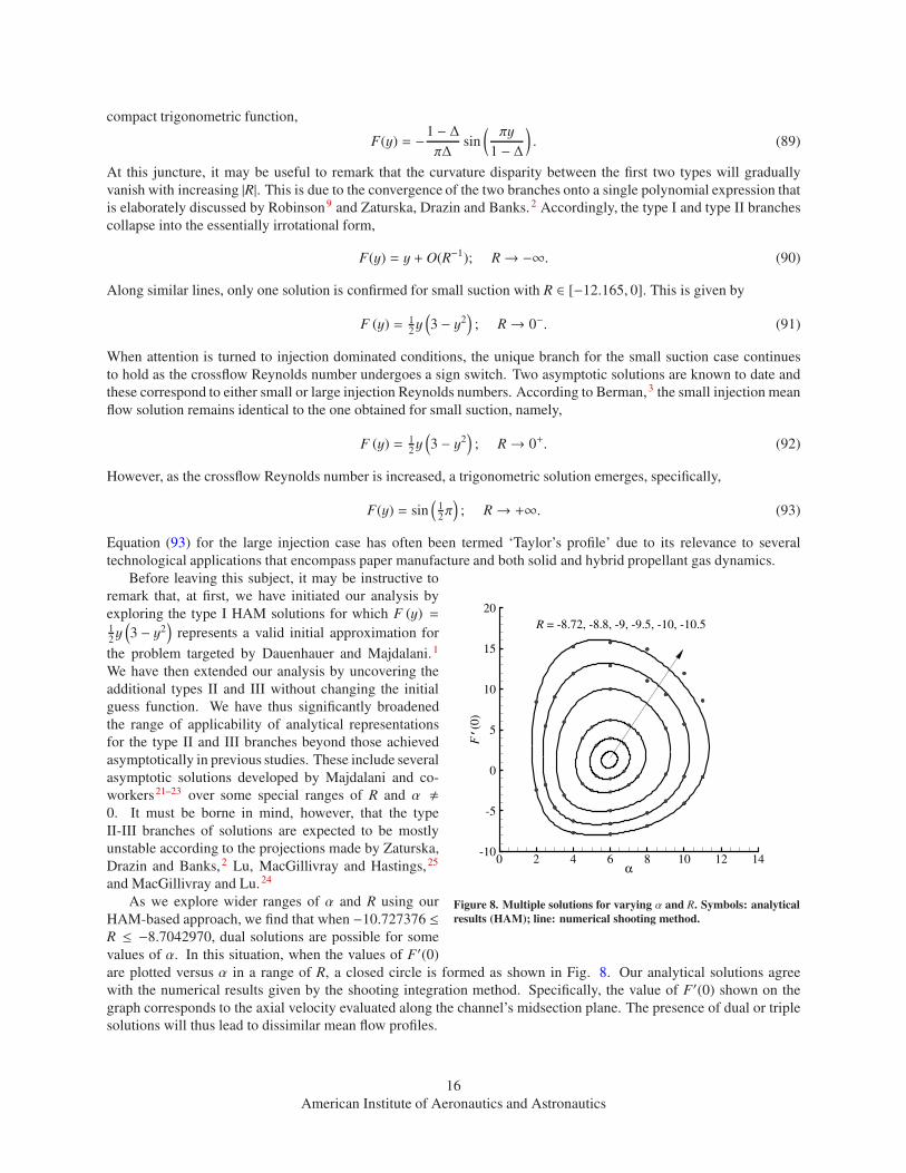
α

F’

(0)

0 2 4 6 8 10 12 14­10

­5

0

5

10

15

20

R = ­8.72, ­8.8, ­9, ­9.5, ­10, ­10.5

Figure 8. Multiple solutions for varying α and R. Symbols: analytical

results (HAM); line: numerical shooting method.

Before leaving this subject, it may be instructive to

remark that, at first, we have initiated our analysis by

exploring the type I HAM solutions for which F (y) =12y(

3 − y2)

represents a valid initial approximation for

the problem targeted by Dauenhauer and Majdalani.1

We have then extended our analysis by uncovering the

additional types II and III without changing the initial

guess function. We have thus significantly broadened

the range of applicability of analytical representations

for the type II and III branches beyond those achieved

asymptotically in previous studies. These include several

asymptotic solutions developed by Majdalani and co-

workers21–23 over some special ranges of R and α ,

0. It must be borne in mind, however, that the type

II-III branches of solutions are expected to be mostly

unstable according to the projections made by Zaturska,

Drazin and Banks,2 Lu, MacGillivray and Hastings,25

and MacGillivray and Lu.24

As we explore wider ranges of α and R using our

HAM-based approach, we find that when −10.727376 ≤

R ≤ −8.7042970, dual solutions are possible for some

values of α. In this situation, when the values of F′(0)

are plotted versus α in a range of R, a closed circle is formed as shown in Fig. 8. Our analytical solutions agree

with the numerical results given by the shooting integration method. Specifically, the value of F′(0) shown on the

graph corresponds to the axial velocity evaluated along the channel’s midsection plane. The presence of dual or triple

solutions will thus lead to dissimilar mean flow profiles.

16

American Institute of Aeronautics and Astronautics

IV. Time-Dependent Wall Regression

The analysis so far has been centered on the assumption that α remains constant during the expanding or

contracting motions of the porous wall. In what follows, we relax this condition and allow the wall expansion ratio to

become time-variant. This enables us to test the validity of the original assumption leading to the exact Navier-Stokes

reduction. Our choice of α(t) is guided by the formulations presented through Eqs. (18)-(21). For example, by taking

α(t) = α0 exp(−t) + α1[1 − exp(−t)], (94)

we obtain

β(t) = −2α0 exp(−t) + 2α1 t + 2α1 exp(−t). (95)

It can thus be seen that the wall expansion ratio α(t) varies exponentially. If we further assume that α0 and α1 represent

the initial and final values of α(t), we can put

α(t) = α1 + (α1 − α0)t

1 + t, (96)

whence

β(t) = 2α1t + 2(α0 − α1) log(1 + t). (97)

In what follows, we find it useful to employ the algebraic approximations, Eqs. (96)-(97), in lieu of the exponentially

decaying forms given by Eqs. (94)-(95). In the present case, we solve a nonlinear PDE, here Eq. (21), with the

boundary conditions given by Eq. (17). In general, a nonlinear PDE is substantially more challenging to solve than

an ODE, even by means of numerical techniques. Besides, PDEs are traditionally regarded as fundamentally different

from ODEs. So the question that comes to mind is this: Can we transform a nonlinear PDE into an infinite number of

linear ODEs? The answer is positive: in many cases, a nonlinear PDE can be indeed broken down into a sequence of

linear ODEs by means of homotopy.30,41 The analytical treatment of a nonlinear, unsteady PDE with a time-dependent

wall expansion ratio α(t) is rather similar to that employed in the treatment of a nonlinear ODE with constant α. The

procedure is straightforward and so, in the interest of brevity, the steps are outlined below and further detailed in the

Appendix. First, F(η, t) is expressed by a series

F(η, t) = F0(η, t) +

+∞∑

m=1

Fm(η, t), (98)

where Fm(η, t) is controlled by the high-order deformation equation

L[

Fm(η, t) − χm Fm−1(η, t)]

= ~ δm(η, t) (99)

with

Fm(0, t) = 0,∂2Fm

∂η2

∣

∣

∣

∣

∣

∣

η=0

= 0, Fm(1, t) = 0,∂Fm

∂η

∣

∣

∣

∣

∣

η=1

= 0, (100)

in which

δm(η, t) = F′′′′m−1 + α(t) (3F′′m−1 + ηF′′′m−1) − β(t) S ′′m−1

+

m−1∑

n=0

(FnF′′′m−1−n + F′nF′′m−i−n). (101)

Here, the primes and dots denote differentiation with respect to η and t, respectively, the auxiliary linear operator L is

the same as in Eq. (51), and χm is defined by Eq. (65). For simplicity, we choose a simple initial guess

F0(η, t) = 12

R η(3 − η2), (102)

which satisfies Eq. (17). Subsequently, the nonlinear PDE defined by Eq. (21) may be converted into an infinite

number of linear ODEs using HAM, as shown in the Appendix.

17

American Institute of Aeronautics and Astronautics

The sensitivity of the solution with respect to the choice of a time-dependent model for α(t) is illustrated in Fig.

9. Therein, the axial velocity profile is plotted at R = 1 and several instants of time that correspond to a variation in

α(t) from −2 to −1. It is interesting to note the general agreement between the two families of curves. As one may

expect, the profiles using the exponentially decaying behavior for α(t) vary slightly more rapidly than those based on

the algebraic approximation. Another case is illustrated in Fig. 10 where the axial velocity profile Fη(0, t) is plotted as

a function of t while α(t) is varied ‘to and fro’ between 1 and 2. It is clear that the velocity decays monotonically when

α(t) is reduced from 2 to 1; the converse is true as α(t) is incremented from 1 to 2. The significant outcome to report

here is that, regardless of direction taken, the velocity profiles quickly approach the steady-state conditions. Similar

trends are displayed by other flow variables. This rapid shift to steady-state behavior helps to confirm the validity

of the analysis performed heretofore, specifically in Sec. III where the time-dependence is deliberately ignored as a

requirement to reduce the Navier-Stokes equations into a single, fourth-order ODE.

η

Fη(η

,t)

0 0.1 0.2 0.3 0.4

1.3

1.4

1.5

1.6

1.7

t =0,

0.25

,1.0

,5

exponential

algebraic

Figure 9. Sensitivity of the axial velocity Fη(η, t) at R = 1 as α(t) is

varied from α0 = −2 to α1 = −1.

t

Fη(0

, t)

0 1 2 3 4 5 6 7 8 9 10­1.65

­1.6

­1.55

­1.5

α0 = 1, α

1 = 2

α0 = 2, α

1 = 1

Figure 10. Temporal variation of the centerline velocity Fη(0, t) for

R = 1.

η

F’

(η,

t)

0 0.1 0.2 0.3 0.4 0.5 0.6 0.7 0.8 0.9 1­8

­7

­6

­5

­4

­3

­2

­1

0

t = 5.0, 10.0

t = 0.0

t = 0.5

t = 2.0

t = 1.0

Solid line: t = 5.0Dash dotted line with symbols: t = 10.0

a) A = −5

η

F’

(η,

t)

0 0.1 0.2 0.3 0.4 0.5 0.6 0.7 0.8 0.9 10

1

2

3

4

5

6

7

8

t = 5.0, 10.0

t = 0.0

t = 0.5

t = 1.0

t = 2.0

Solid line: t = 5.0Dash dotted line with symbols: t = 10.0

b) A = 5

Figure 11. Spatial variation of the axial velocity Fη(η, t) for some values of t using a) A = −5 and b) A = 5.

18

American Institute of Aeronautics and Astronautics

η

F(η

)/R

­1 ­0.8 ­0.6 ­0.4 ­0.2 0 0.2 0.4 0.6 0.8 1­1

­0.8

­0.6

­0.4

­0.2

0

0.2

0.4

0.6

0.8

1

α = 5α = 0α =­5

Figure 12. Spatial variation of the normal velocity profile F(η)/Rusing a 40th-order HAM approximation and three fixed values of

α and R = 5.

η

F(η

,t)

­1 ­0.8 ­0.6 ­0.4 ­0.2 0 0.2 0.4 0.6 0.8 1­6

­4

­2

0

2

4

6

t = 0

.0, 0

.5, 1

.0, 2

.0, 5

.0

Figure 13. Spatial variation of the normal velocity F(η, t) using a

[30,30] order homotopy-Pade approximation for some values of t

and A = 5. Here α(t) evolves exponentially from −1 to −2.

To illustrate the time-dependent evolution of the axial velocity, Figs. 11a and 11b are used to depict the behavior

of F′ at two different injection coefficients, specifically, for A = ±5. These results correspond to the direct temporal

solution of Eq. (21). To verify the rapid shift to steady-state conditions, the axial velocity profiles are shown for

t = 0, 0.5, 1.0, 2.0, 5.0, 10.0. Note that, at the scale used in these graphs, the curves beyond t = 5 cannot be visually

distinguished. Along similar lines, the spatial variation of the normal velocity is illustrated in Figs. 12 and 13. In Fig.

12, the sensitivity of the normal velocity is illustrated at three different wall expansion ratios, α = −5, 0,+5, hence

including those caused by suction, stationary motion, or injection. These are computed using a 40th-order HAM

approximation and a fixed crossflow Reynolds number of R = 5. As for Fig. 13, it illustrates the time-evolution of

the normal velocity for t = 0, 0.5, 1.0, 2.0, 5.0, an injection coefficient of A = 5 and a time-dependent wall expansion

ration that varies from −1 to −2. Here too, results beyond t = 5.0 become indiscernible, thus signaling the onset of

steady-state conditions.

V. Conclusions

In this study, the porous channel with orthogonally moving walls is revisited in the context of laminar

incompressible motion with both uniform and non-uniform wall regression. The flow in the case of uniform wall

regression is described by a nonlinear ODE, but the flow in the case of non-uniform wall regression is prescribed by

a nonlinear PDE. For each case, an analytic approach based on the Homotopy Analysis Method (HAM) is presented,

thus transforming the original nonlinear ODE or PDE into an infinite number of linear ODEs whose solutions can

be obtained by symbolic computation software. At the outset, a recursive series formulation is derived that can be

readily evaluated using generic programming. The HAM-based procedure may thus be viewed as a technique that

can greatly simplify the solution of nonlinear ODEs or PDEs. In this endeavor, multiple solutions may be connected

to a finite number of distinct zeroes, here called γ∗, of a constraint equation associated with the shooting approach.

After identifying the distinct solutions associated with each zero, a convergence-control parameter ~ may be carefully

selected to ensure the convergence of the series at hand. In the present work, an error minimization approach is

employed to determine an optimal value, ~∗, that leads to fast series convergence. When necessary, the homotopy-

Pade technique is invoked to further accelerate series convergence. At length, a series approximation is obtained for

the nonlinear Dauenhauer-Majdalani ODE, in the case of constant wall expansion, and for the time-dependent PDE,

in the case of a time-varying wall expansion.

For the uniform wall expansion ratio, our HAM-based approach is shown to capture dual and triple solutions in

different ranges of R and α. We not only recover the type I branch of solutions pursued by Dauenhauer and Majdalani,

19

American Institute of Aeronautics and Astronautics

1 but also capture the type II and type III families reported by Zaturska, Drazin and Banks.2 These solutions were

alluded to although not pursued in Dauenhauer and Majdalani’s former article.1 The new profiles involve either steeper

flow turning at the wall (type II) or annular flow splitting and recirculation that are thoroughly described by Lu (type

III). The high-order approximations presented here to describe all three categories of motion are shown to exhibit

substantial agreement with the numerical results acquired using the integration algorithm constructed by Dauenhauer

and Majdalani.1

For the non-uniform wall expansion case, two models for α(t) are chosen that involve either exponential or

algebraic variation from an initial α0 to a final α1. With this assumption in effect, the Navier-Stokes equations are

transformed into a partial differential equation using a judicious choice of similarity variables. The resulting problem

is solved analytically by HAM and shown to quickly reproduce the steady-state solution obtained previously. This

is due to the rapid decay of the time-dependent transients and the swift convergence of the solution to conditions

corresponding to a constant wall expansion ratio.

Finally, it is clear that HAM offers several advantages when compared to other methods of solution. Firstly, while

the reduced ODE has been previously solved using asymptotics, its accuracy has remained dependant on the size

of the small perturbation parameter 1/R. Unlike the perturbation approximation that applies to a limited range of

Reynolds numbers, the HAM solution has no limitations. It is not only independent of the size of 1/R but it also

provides, as a windfall, a convenient tool that can be calibrated to ensure series convergence. Secondly, the process of

identifying multiple solutions using HAM is facilitated, even in the case for which the multiplicity in the numerical

solution becomes elusive. Thirdly, the solution of the nonlinear PDE is made possible through the use of HAM,

which could deal with both nonlinear ODEs and nonlinear PDEs with equal level of ease. The main benefits of HAM

stand, perhaps, in its ability to solve a nonlinear equation using a parameter-free procedure that is so versatile that it

can handle equally efficiently either a PDE or an ODE. Using similar tactics, our analytical approach can be further

applied and incrementally modified to help in the identification of multiple steady and time-dependent solutions of a

variety of nonlinear equations that arise in fluid mechanics, especially in the field of global flow stability.

Appendix: Procedure for Solving the Unsteady Wall Regression Problem

In what follows, we describe the mathematical steps needed to apply the Homotopy Analysis Method to the porous

channel flow problem with a time-dependent expansion ratio α(t). We thus consider the unsteady PDE given by Eq.

(21). The attendant analysis encompasses the solution to Eq. (16), which can be recovered for α(t) = 12, β(t) =

constant. The description to follow can thus be applied to both steady and unsteady cases.

To begin, the form of the analytical solutions to Eq. (21) must be posited in term of suitable functions. Depending

on the character of β(t) or α(t), different solution expressions are required. For the type I family of solutions that we

seek here, three cases arise depending on the behavior of α(t). For α(t) = constant, F becomes independent of time;

nonetheless, to present the procedure systematically for the three cases at hand, we still include t as we put

F(η, t) =

+∞∑

i=0

Biηi. (103)

Next, we consider the unsteady α(t) = α0 exp(−t) + α1[1 − exp(−t)]; the solution expression for the exponentially

decaying behavior may be readily expressed as

F(η, t) =

∞∑

i=0

∞∑

j=0

∞∑

k=0

Bki, j η

i t j exp(−k t). (104)

Finally, for α(t) = α1 + (α1 − α0)t/(1 + t), the series representation for the algebraically varying expansion ratio may

be written as

F(η, t) =

∞∑

i=0

∞∑

j=0

∞∑

k=0

∞∑

s=0

Bk,si, j η

i t j 1

(1 + x)k[ln(1 + t)]s. (105)

Here Bi, Bki, j, and B

k,si, j are undetermined coefficients that we must seek to determine.

According to the homotopy-based approach, one needs to introduce an initial guess function of the form prescribed

by the solution expressions while satisfying the problem’s boundary conditions. For all three cases, a suitable choice

20

American Institute of Aeronautics and Astronautics

corresponds to the leading order asymptotic solution obtained by Berman3 at small Reynolds numbers, specifically,

φ0(η, t) = 12R η(3 − η2). (106)

Note that the above satisfies Eq. (11) and may be shown to be a viable candidate for the initial approximation of

F(η, t). An auxiliary linear operatorL is then defined to the extent of capturing the highest order in Eq. (21). This is

L[Φ(η, t)] =∂4Φ(η, t)

∂η4, (107)

which has the property

L(C0 +C1η + C2η2 +C3η

3) = 0, (108)

where (C0,C1,C2,C3) are integral constants. This representation satisfies the rule of solution expression through which

the linear approximation is constructed from the set of base functions. At this point, a homotopy mapping relation

may be implemented of the type

F : η, t × [0, 1] 7−→ H|Φ(η, t; 0) = φ(η, t); Φ(η, t; 1) = F(η, t). (109)

This transformation leads to the HAM deformation equation that has been well established as

(1 − q)L[Φ(η, t; q) − φ0(η, t)] = q ~ N[Φ(η, t; q)], (110)

where q ∈ [0, 1] is an embedding parameter and ~ is a non-zero auxiliary parameter known as the convergence-control

parameter.27 Note that N is a nonlinear operator obtained by recasting Eq. (21) into N[Φ(η; q)] = 0. We therefore

have

N[Φ(η; q)] =∂4Φ(η; q)

∂η4+ Φ(η; q)

∂3Φ(η; q)

∂η3+

3

2βt(t)

∂2Φ(η; q)

∂η2

−∂Φ(η; q)

∂η

∂2Φ(η; q)

∂η2+

1

2βt(t) η

∂3Φ(η; q)

∂η3− β(t)

∂3Φ(η; q)

∂η2∂t. (111)

The corresponding assortment of boundary conditions translates into

Φ(0, t; q) = 0,∂2Φ(η, t; q)

∂η2

∣

∣

∣

∣

∣

∣

η=0

= 0, Φ(1, t; q) = R,∂Φ(η, t; q)

∂η

∣

∣

∣

∣

∣

η=1

= 0. (112)

At this point, it may be instructive to note that when

q = 0 : L[Φ(η, t; 0) − φ0(η, t)] = 0,

q = 1 : N[Φ(η, t; 1)] = 0; ∀~ , 0.(113)

Hence as we track the evolution of q across the range [0,1], the solution of the nonlinear equation will transition from

the initial approximation φ0(η) to the target function that will exactly satisfy Eq. (21). Expanding Φ(η, t; q) in the

MacLaurin series form with respect to q, we have

Φ(η, t; q) = Φ0(η, t, 0) +

+∞∑

m=1

φm(η, t) qm, (114)

where

φm(η, t) =1

m!

∂mΦ(η, t; q)

∂qm

∣

∣

∣

∣

∣

q=0

. (115)

For brevity, we introduce a vector

~φm = φ0(η, t), φ1(η, t), φ2(η, t), · · · , φm(η, t). (116)

21

American Institute of Aeronautics and Astronautics

The next step consists of differentiating the HAM deformation equation (110) m times with respect to q, dividing by

m!, and then setting q = 0. This enables us to obtain the mth-order deformation equation

L[φm(η, t) − χmφm−1(η, t)] = ~ Rm[φm−1(η, t)], (117)

which is subject to the boundary conditions

η = 0 : φm = 0, φ′′m = 0; η = 1 : φm = 0, φ′m = 0. (118)

In Eq. (117), the right-hand-side function Rm is given by

Rm[φm−1(η, t)] =1

(m − 1)!

∂m−1N[Φ(η, t; q)]

∂qm−1

∣

∣

∣

∣

∣

∣

q=0

= φ′′′′m−1 +

m−1∑

i=0

(φiφ′′′m−1−i + φ

′iφ′′m−i−i)

+ 12βt(t)(3φ

′′m−1+ ηφ′′′

m−1) − β(t)φ′′t m−1, (119)

where the prime denotes differentiation with respect to η.

By substituting the form of Eq. (108), the general solution for Eq. (117) can be extracted. Using φ∗m(η, t) to denote

a particular solution of Eq. (117), one collects

φm(η, t) = χmφm−1(η, t) + φ∗m(η, t) +Cm0 +Cm

1 η +Cm2 η

2 +Cm3 η

3 (m > 0), (120)

where Cm0

, Cm1

, Cm2

and Cm3

can be determined from the boundary conditions in Eq. (118). After some algebra, one gets

Cm0 = −φ

∗m(0, t), Cm

1 = −φ∗m(1, t) − Cm

0 − Cm2 − Cm

3 ,

Cm2 = −

1

2φ∗m′′

(0, t), Cm3 =

1

2[φ∗m(1, t) − φ∗m

′(1, t) + Cm

0 + Cm2 ]. (121)

It can thus be seen that the linear relation (117) may be solved recursively, one order at a time, for m = 1, 2, 3, . . . .

We now recall that, according to the definition (107) of L, the high-order deformation equation (63) is linear. Then

following the HAM procedure, a nonlinear PDE, such as Eq. (21), may be transformed into an infinite number of

linear ODEs. The present approach guarantees the convergence of the series solution by providing the freedom to

select a suitable convergence-control parameter ~ or to use the homotopy-Pade technique.28–31

Acknowledgments

At one end, Dr. Majdalani is deeply grateful for the hospitality received from Drs. Jie-Zhi Wu, Zhen-Su She, and

Shi-Yi Chen of Peking University. Moreover, he is immensely thankful for NSF grants No. 0353518 and 0928762,

and most appreciative of their Program Directors, Drs. Masayoshi Tomizuka, Eduardo A. Misawa, and Win Aung. At

the other end, Drs. Xu, Lin and Liao are thankful for NSFC grants No. 10972036, 50739004 and 10872129 received

from the National Natural Science Foundation of China. Finally, Dr. Liao acknowledges the partial support derived

from the State Key Laboratory of Ocean Engineering through grant No. GKZD010002.

References

1Dauenhauer, E. C., and Majdalani, J., “Exact Self-Similary Solutionof the Navier-stokes Equations for a Porous Channel with Orthogonally

Moving Walls,” The Physics of Fluids, Vol. 15, No. 6, 2003, pp. 1485–1495. doi:10.1063/1.1567719.2Zaturska, M. B., Drazin, P. G., and Banks, W. H., “On the Flow of a Viscous Fluid Driven Along a Channel by Suction at Porous Walls,”

Fluid Dynamics Research, Vol. 4, No. 3, 1988, pp. 151–178. doi:10.1016/0169-5983(88)90021-4.3Berman, A. S., “Laminar Flow in Channels with Porous Walls,” Journal of Applied Physics, Vol. 24, No. 9, 1953, pp. 1232–1235.

doi:10.1063/1.1721476.4Terrill, R. M., “Laminar Flow in a Uniformly Porous Channel,” The Aeronautical Quarterly, Vol. 15, 1964, pp. 299–310.5Morduchow, M., “On Laminar Flow Through a Channel or Tube with Injection: Application of Method of Averages,” Quarterly Journal of

Applied Mathematics, Vol. 14, No. 4, 1957, pp. 361–368.6White, F. M., Barfield, B. F., and Goglia, M. J., “Laminar Flow in a Uniformly Porous Channel,” Transactions of the American Society of

Mechanical Engineers: Journal of Applied Mechanics, Vol. 25, 1958, pp. 613–617.

22

American Institute of Aeronautics and Astronautics

7Sellars, J. R., “Laminar Flow in Channels with Porous Walls at High Suction Reynolds Numbers,” Journal of Applied Physics, Vol. 26,

No. 4, 1955, pp. 489–490. doi:10.1063/1.1722024.8Shrestha, G. M., “Singular Perturbation Problems of Laminar Flow in a Uniformly Porous Channel in the Presence of a Transverse Magnetic

Field,” Quarterly Journal of Mechanics and Applied Mathematics, Vol. 20, No. 2, 1967, pp. 233–246. doi:10.1093/qjmam/20.2.233.9Robinson, W. A., “The Existence of Multiple Solutions for the Laminar Flow in a Uniformly Porous Channel with Suction at both Walls,”

Journal of Engineering Mathematics, Vol. 10, No. 1, 1976, pp. 23–40. doi:10.1007/BF01535424.10Skalak, F. M., and Wang, C. Y., “On the Nonunique Solutions of Laminar Flow Through a Porous Tube or Channel,” SIAM Journal on

Applied Mathematics, Vol. 34, No. 3, 1978, pp. 535–544. doi:10.1137/0134042.11Brady, J. F., “Flow Development in a Porous Channel and Tube,” The Physics of Fluids, Vol. 27, No. 5, 1984, pp. 1061–1067.

doi:10.1063/1.864735.12Durlofsky, L., and Brady, J. F., “The Spatial Stability of a Class of Similarity Solutions,” The Physics of Fluids, Vol. 27, No. 5, 1984,

pp. 1068–1076. doi:10.1063/1.864736.13Taylor, G. I., “Fluid Flow in Regions Bounded by Porous Surfaces,” Proceedings of the Royal Society of London, Series A, Vol. 234, No.

1199, 1956, pp. 456–475. doi:10.1098/rspa.1956.0050.14Yuan, S. W., “Further Investigation of Laminar Flow in Channels with Porous Walls,” Journal of Applied Physics, Vol. 27, No. 3, 1956,

pp. 267–269. doi:10.1063/1.1722355.15Proudman, I., “An Example of Steady Laminar Flow at Large Reynolds Number,” Journal of Fluid Mechanics, Vol. 9, No. 4, 1960, pp. 593–

602. doi:10.1017/S002211206000133X.16Terrill, R. M., and Shrestha, G. M., “Laminar Flow Through Parallel and Uniformly Porous Walls of Different Permeability,” Zeitschrift fr

angewandte Mathematik und Physik, Vol. 16, No. 4, 1965, pp. 470–482. doi:10.1007/BF01593923.17Shrestha, G. M., and Terrill, R. M., “Laminar Flow with Large Injection Through Parallel and Uniformly Porous Walls of Different

Permeability,” Quarterly Journal of Mechanics and Applied Mathematics, Vol. 21, No. 4, 1968, pp. 413–432. doi:10.1093/qjmam/21.4.413.18Brady, J. F., and Acrivos, A., “Steady Flow in a Channel or Tube with an Acceleration Surface Velocity: An Exact Solution to the Navier-

Stokes Equations with Reverse Flow,” Journal of Fluid Mechanics, Vol. 112, No. 5, 1981, pp. 127–150. doi:10.1017/S0022112081000323.19Watson, E., Banks, W. H., Zaturska, M. B., and Drazin, P. G., “On Transition to Chaos in Two-Dimensional Channel Flow Symmetrically

Driven by Accelerating Walls,” Journal of Fluid Mechanics, Vol. 212, No. 1, 1991, pp. 451–485. doi:10.1017/S0022112090002051.20Watson, P., Banks, W. H., Zaturska, M. B., and Drazin, P. G., “Laminar Channel Flow Driven by Accelerating Walls,” European Journal of

Applied Mathematics, Vol. 2, No. 4, 1991, pp. 359–385. doi:10.1017/S0956792500000607.21Majdalani, J., and Zhou, C., “Moderate-to-Large Injection and Suction Driven Channel Flows with Expanding or Contracting Walls,”

Zeitschrift fr angewandte Mathematik und Mechanik, Vol. 83, No. 3, 2003, pp. 181–196. doi:10.1002/zamm.200310018.22Majdalani, J., Zhou, C., and Dawson, Christopher, A., “Two-Dimensional Viscous Flow Between Slowly Expanding or Contracting Walls

with Weak Permeability,” Journal of Biomechanics, Vol. 35, No. 10, 2002, pp. 1399–1403. doi:10.1016/S0021-9290(02)00186-0.23Zhou, C., and Majdalani, J., “Improved Mean Flow Solution for Slab Rocket Motors with Regressing Walls,” Journal of Propulsion and

Power, Vol. 18, No. 3, 2002, pp. 703–711. doi:10.2514/2.5987.24MacGillivray, A. D., and Lu, C., “Asymptotic Solution of a Laminar Flow in a Porous Channel with Large Suction: A Nonlinear Turning

Point Problem,” Methods and Applications of Analysis, Vol. 1, No. 2, 1994, pp. 229–248.25Lu, C., MacGillivray, A. D., and Hastings, S. P., “Asymptotic Behaviour of Solutions of a Similarity Equation for Laminar Flows in Channels

with Porous Walls,” IMA Journal of Applied Mathematics, Vol. 49, No. 2, 1992, pp. 139–162. doi:10.1093/imamat/49.2.139.26Cox, S. M., and King, A. C., “On the Asymptotic Solution of a High-Order Nonlinear Ordinary Differential Equation,” Proceedings of the

Royal Society of London, Series A, Vol. 453, No. 1959, 1997, pp. 711–728. doi:10.1098/rspa.1997.0040.27Liao, S., “Notes on the Homotopy Analysis Method: Some Definitions and Theorems,” Communications in Nonlinear Science and

Numerical Simulation, Vol. 14, No. 4, 2009, pp. 983–997. doi:10.1016/j.cnsns.2008.04.013.28Liao, S. J., “A Kind of Approximate Solution Technique Which Does Not Depend upon Small Parameters–II. An Application in Fluid

Mechanics,” International Journal for Nonlinear Mechanics, Vol. 32, No. 5, 1997, pp. 815–822. doi:10.1016/s0020-7462(96)00101-1.29Liao, S., Beyond Perturbation: Introduction to the Homotopy Analysis Method, Chapman & Hall/ CRC Press, 2003.30Liao, S., and Tan, Y., “A General Approach to Obtain Series Solutions of Nonlinear Differential Equations,” Studies in Applied Mathematics,

Vol. 119, No. 4, 2007, pp. 297–354. doi:10.1111/j.1467-9590.2007.00387.x.31Liao, S., “On the Homotopy Analysis Method for Nonlinear Problems,” Applied Mathematics and Computation, Vol. 147, No. 2, 2004,

pp. 499–513. doi:10.1016/S0096-3003(02)00790-7.32Xu, H., Liao, S. J., and Pop, I., “Series Solution of Unsteady Boundary Layer Flows of Non-Newtonian Fluids near a Forward Stagnation

Point,” Journal of Non-Newtonian Fluid Mechanics, Vol. 139, No. 1-2, 2006, pp. 31–43. doi:10.1016/j.jnnfm.2006.06.003.33Xu, H., Liao, S. J., and Pop, I., “Series Solutions of Unsteady Three-Dimensional MHD Flow and Heat Transfer in the

Boundary Layer over an Impulsively Stretching Plate,” European Journal of Mechanics, B/Fluids, Vol. 26, No. 1, 2007, pp. 15–27.

doi:10.1016/j.euromechflu.2005.12.003.34Abbasbandy, S., “The Application of the Homotopy Analysis Method to Nonlinear Equations Arising in Heat Transfer,” Physics Letters A,

Vol. 360, No. 1, 2006, pp. 109–113. doi:10.1016/j.physleta.2006.07.065.35Yabushita, K., Yamashita, M., and Tsuboi, K., “An Analytic Solution of Projectile Motion with the Quadratic Resistance Law

Using the Homotopy Analysis Method,” Journal of Physics A: Mathematical and Theoretical, Vol. 40, No. 29, 2007, pp. 8403–8416.

doi:10.1088/1751-8113/40/29/015.36Song, H., and Tao, L., “Homotopy Analysis of 1D Unsteady, Nonlinear Groundwater Flow Through Porous Media,” Journal of Coastal

Research, Vol. 50, 2007, pp. 292–296.37Hayat, T., and Sajid, M., “Homotopy Analysis of MHD Boundary Layer Flow of an Upper-Convected Maxwell Fluid,” International Journal

of Engineering Science, Vol. 45, No. 2–8, 2007, pp. 393–401. doi:10.1016/j.ijengsci.2007.04.009.38Allan, F., “Derivation of the Adomian Decomposition Method Using the Homotopy Analysis Method,” Applied Mathematics and

Computation, Vol. 190, No. 1, 2007, pp. 6–14. doi:10.1016/j.amc.2006.12.074.

23

American Institute of Aeronautics and Astronautics

39Wu, Y., and Cheung, K., “Explicit Solution to the Exact Riemann Problems and Application in Nonlinear Shallow-Water Equations,”

International Journal for Numerical Methods in Fluids, Vol. 57, No. 11, 2008, pp. 1649–1668. doi:10.1002/fld.1696.40White, F., Viscous Fluid Flow, McGraw-Hill, New York, 1991, 135–136.41Liao, S., “A General Approach to Get Series Solution of Non-Similarity Boundary Layer Flows,” Communications in Nonlinear Science

and Numerical Simulation, Vol. 14, No. 5, 2009, pp. 2144–2159. doi:10.1016/j.cnsns.2008.06.013.42Lu, C., “On the Asymptotic Solution of Laminar Channel Flow with Large Suction,” SIAM Journal on Mathematical Analysis, Vol. 28,

No. 5, 1997, pp. 1113–1134. doi:10.1137/S0036141096297704.

24

American Institute of Aeronautics and Astronautics