EVOLVING INTELLIGENT SYSTEMS

EVOLVING INTELLIGENTSYSTEMS

IEEE Press

445 Hoes Lane

Piscataway, NJ 08854

IEEE Press Editorial Board

Lajos Hanzo, Editor in Chief

R. Abari T. Chen B. M. Hammerli

J. Anderson T. G. Croda O. Malik

S. Basu M. El-Hawary S. Nahavandi

A. Chatterjee S. Farshchi W. Reeve

Kenneth Moore, Director of IEEE Book and Information Services (BIS)

IEEE-CIS Liaison to IEEE Press, Gary B. Fogel

Books in the IEEE Press Series on Computational Intelligence

Introduction to Evolvable Hardware: A Practical Guide for Designing Self-Adaptive Systems

Garrison W. Greenwood and Andrew M. Tyrrell

2007 978-0471-71977-9

Evolutionary Computation: Toward a New Philosophy of Machine Intelligence, Third Edition

David B. Fogel

2006 978-0471-66951-7

Emergent Information Technologies and Enabling Policies for Counter-Terrorism

Edited by Robert L. Popp and John Yen

2006 978-0471-77615-4

Computationally Intelligent Hybrid Systems

Edited by Seppo J. Ovaska

2005 978-0471-47668-4

Handbook of Learning and Appropriate Dynamic Programming

Edited by Jennie Si, Andrew G. Barto, Warren B. Powell, Donald Wunsch II

2004 978-0471-66054-X

Computational Intelligence: The Experts Speak

Edited by David B. Fogel and Charles J. Robinson

2003 978-0471-27454-2

Computational Intelligence in Bioinformatics

Edited by Gary B. Fogel, David W. Corne, and Yi Pan

2008 978-0470-10526-9

Computational Intelligence and Feature Selection: Rough and Fuzzy Approaches

Richard Jensen and Qiang Shen

2008 978-0470-22975-0

Clustering

Rui Xu and Donald C. Wunsch II

2009 978-0470-27680-8

EVOLVING INTELLIGENTSYSTEMS

Methodology andApplications

EDITED BY

Plamen AngelovDimitar P. FilevNikola Kasabov

Copyright � 2010 by Institute of Electrical and Electronics Engineers. All rights reserved.

Published by John Wiley & Sons, Inc., Hoboken, New Jersey.

Published simultaneously in Canada.

No part of this publication may be reproduced, stored in a retrieval system, or transmitted in any form or by

any means, electronic, mechanical, photocopying, recording, scanning, or otherwise, except as permitted

under Section 107 or 108 of the 1976 United States Copyright Act, without either the prior written

permission of the Publisher, or authorization through payment of the appropriate per-copy fee to the

Copyright Clearance Center, Inc., 222 Rosewood Drive, Danvers, MA 01923, (978) 750-8400, fax (978)

750-4470, or on the web at www.copyright.com. Requests to the Publisher for permission should be

addressed to the Permissions Department, John Wiley & Sons, Inc., 111 River Street, Hoboken, NJ 07030,

(201) 748-6011, fax (201) 748-6008, or online at http://www.wiley.com/go/permission.

Limit of Liability/Disclaimer of Warranty: While the publisher and author have used their best efforts in

preparing this book, they make no representations or warranties with respect to the accuracy or completeness

of the contents of this book and specifically disclaim any implied warranties of merchantability or fitness for

a particular purpose. No warranty may be created or extended by sales representatives or written sales

materials. The advice and strategies contained herein may not be suitable for your situation. You should

consult with a professional where appropriate. Neither the publisher nor author shall be liable for any loss of

profit or any other commercial damages, including but not limited to special, incidental, consequential, or

other damages

For general information on our other products and services or for technical support, please contact our

Customer Care Department within the United States at (800) 762-2974, outside the United States at (317)

572-3993 or fax (317) 572-4002

Wiley also publishes its books in a variety of electronic formats. Some content that appears in print may not

be available in electronic formats. For more information about Wiley products, visit our web site at

www.wiley.com

Library of Congress Cataloging-in-Publication Data:

Evolving intelligent systems : methodology and applications / Plamen Angelov, Dimitar P. Filev,

Nik Kasabov.

p. cm.

Includes index.

ISBN 978-0-470-28719-4 (cloth)

1. Computational intelligence. 2. Fuzzy systems. 3. Neural networks (Computer science)

4. Evolutionary programming (Computer science) 5. Intelligent control systems.

I. Angelov, Plamen. II. Filev, Dimitar P., 1959- III. Kasabov, Nikola K.

Q342.E785 2009

006.3–dc20

2009025980

Printed in the United States of America.

10 9 8 7 6 5 4 3 2 1

CONTENTS

PREFACE vii

1 LEARNING METHODS FOR EVOLVING INTELLIGENT SYSTEMS 1

Ronald R. Yager

2 EVOLVING TAKAGI-SUGENO FUZZY SYSTEMS FROMSTREAMING DATA (eTSþ ) 21Plamen Angelov

3 FUZZY MODELS OF EVOLVABLE GRANULARITY 51

Witold Pedrycz

4 EVOLVING FUZZY MODELING USING PARTICIPATORY LEARNING 67

E. Lima, M. Hell, R. Ballini, F. Gomide

5 TOWARD ROBUST EVOLVING FUZZY SYSTEMS 87

Edwin Lughofer

6 BUILDING INTERPRETABLE SYSTEMS IN REAL TIME 127

Jos�e V. Ramos, Carlos Pereira, Antonio Dourado

7 ONLINE FEATURE EXTRACTION FOR EVOLVINGINTELLIGENT SYSTEMS 151S. Ozawa, S. Pang, N. Kasabov

8 STABILITY ANALYSIS FOR AN ONLINE EVOLVING NEURO-FUZZYRECURRENT NETWORK 173Jos�e de Jesus Rubio

9 ONLINE IDENTIFICATION OF SELF-ORGANIZING FUZZY NEURALNETWORKS FOR MODELING TIME-VARYING COMPLEX SYSTEMS 201G. Prasad, G. Leng, T.M. McGinnity, D. Coyle

10 DATA FUSION VIA FISSION FOR THE ANALYSIS OF BRAIN DEATH 229

L. Li, Y. Saito, D. Looney, T. Tanaka, J. Cao, D. Mandic

11 SIMILARITY ANALYSIS AND KNOWLEDGE ACQUISITION BYUSE OF EVOLVING NEURAL MODELS AND FUZZY DECISION 247Gancho Vachkov

12 AN EXTENDED VERSION OF THE GUSTAFSON-KESSELALGORITHM FOR EVOLVING DATA STREAM CLUSTERING 273Dimitar Filev, Olga Georgieva

13 EVOLVING FUZZY CLASSIFICATION OF NONSTATIONARYTIME SERIES 301Ye. Bodyanskiy, Ye. Gorshkov, I. Kokshenev, V. Kolodyazhniy

14 EVOLVING INFERENTIAL SENSORS IN THE CHEMICALPROCESS INDUSTRY 313Plamen Angelov, Arthur Kordon

15 RECOGNITION OF HUMAN GRASP BY FUZZY MODELING 337

R. Palm, B. Kadmiry, B. Iliev

16 EVOLUTIONARY ARCHITECTURE FOR LIFELONG LEARNINGAND REAL-TIME OPERATION IN AUTONOMOUS ROBOTS 365R. J. Duro, F. Bellas, J. A. Becerra

17 APPLICATIONS OF EVOLVING INTELLIGENT SYSTEMSTO OIL AND GAS INDUSTRY 401Jos�e Macıas-Hern�andez, Plamen Angelov

Epilogue 423

About the Editors 425

About the Contributors 427

Index 439

vi CONTENTS

PREFACE

One of the consequences of the information revolution is the ever-growing amount of

information we are surrounded with and the need to process this information

efficiently and extract meaningful knowledge. This phenomenon was termed “digital

obesity” or “information obesity” by Toshiba Ltd. One of the specifics of this

phenomenon is that the information not only is presented in huge quantities, but

also is dynamic, presented in a form of streams of data. The latter brings new

challenges to the established approaches to processing data, usually in an offline and

stationary form. To address the new challenges of extracting highly interpretable

knowledge from streams of data, online techniques and methodologies have been

developed, so that a higher level of adaptation, compared to conventional adaptive

systems known from control theory (Astrom & Wittenmark, 1989), is achieved.

These new modeling methods are also principally different from the classical system

identification theory (Ljung, 1988). They differ also from the traditional machine

learning and statistical learning methods (Hastie et al., 2001), where the processes

are usually assumed to have Gaussian distribution and random nature. Evolving

intelligent systems (EISs) are based on fuzzy and neuro-fuzzy techniques that allow

for the structure and the functionality of a system to develop and evolve from

incoming data. They represent a fuzzy mixture of locally valid simpler systems,

which in combination are highly nonlinear and non-Gaussian. They can be considered

fuzzy mixtures of Gaussians, but these mixtures are not pre-fixed and are adapting/

evolving to capture the real data density distribution (Angelov & Zhou, 2008).

A computer, engineering, or any other system that possess features of compu-

tational intelligence is commonly called an intelligent system. Many intelligent

products such as camcorders, washing machines, games, and so on have reached

the market. Once created/designed, however, most of them do not continue to learn,

to improve, and to adapt. This edited volume aims to bring together the best recent

works in the newly emerging subtopic of the area of computational intelligence,

which puts the emphasis on lifetime self-adaptation, and on the online process

of evolving the system’s structure and parameters. Evolving systems can have

different technical or physical embodiments, including intelligent agents, embedded

systems, and ubiquitous computing. They can also have different computational

frameworks, for example, one of a fuzzy rule-based type; one of a neural network

type; one of a multimodel type. The important feature that any EIS possesses is the

ability to:

. Expand or shrink its structure, as well as to adapt its parameters, and thus to evolve

. Work and adapt incrementally, online, and, if necessary, in real time

The newly emerging concept of dynamically evolving structures, which was to

some extent already applied to neural networks (Fritzke, 1994), brought powerful new

concepts of evolving fuzzy systems (Angelov, 2002; Angelov & Filev, 2004; Angelov

and Zhou, 2006) and evolving neuro-fuzzy systems (Kasabov, 2002; 2007), which

together with some other techniques of computational intelligence and statistical

analysis are considered to be EIS (Angelov & Kasabov 2006; Yager, 2006). EIS

combines the interpolation abilities of the (neuro-)fuzzy systems and their flexibility

with the adaptive feature of the online learning techniques. Evolving fuzzy systems

(EFSs), in particular, have the additional advantage of linguistic interpretability and can

be used for extracting knowledge in the form of atomic information granules (linguistic

terms represented by fuzzy sets) (Angelov, 2002; Pedrycz, 2005; Zadeh, 1975) and

fuzzy rules. Neuro-fuzzy systems have also a high degree of interpretability due to their

fuzzy component (Kasabov, 1996; Wang & Mendel, 1992).

One can formulate EIS as a synergy between systems with expandable (evolvable)

structures for information representation (usually these are fuzzy or neuro-fuzzy

structures, but not necessarily) and online methods for machine learning (Lima

et al., 2006; Yager, 2006). The area of EIS is concerned with nonstationary processes,

computationally efficient algorithms for real-time applications, and a dynamically

evolving family of locally valid subsystems that can represent different situations or

operating conditions. The overall global functioning of an EIS is a result of much simpler

local subsystems implementing the philosophical observation by the British mathema-

tician Alan Turing, who said, “The Global order emerges from the chaos of local

interactions.” EISs aim at lifelong learning and adaptation and self-organization

(including system structure evolution) in order to adapt to unknown and unpredictable

environments. EISs also address the problems of detecting temporal shifts and drifts in

the data patterns, adapting the learning scheme itself in addition to the evolution of the

structure and parameters of the system.

This new topic of EIS has marked a significant growth during the past couple of

years, which has led to a range of IEEE-supported events: symposia and workshops

(IEEE IS2002, EFS06, GEFS08, NCEI2008/ICONIP2008, ESDIS2009, EIS2010);

tutorials; special sessions at leading IEEE events (FUZZ-IEEE/IJCNN 2004, NAFIPS

2005,WCCI2006, FUZZ-IEEE2007, IJCNN2007, IEEE-SMC2007, SSCI 2007, FUZZ-

IEEE2007, IPMU2008, IEEE-IS2008, EUSFLAT/IFSA 2009, IPMU2010,WCCI-2010),

and so forth. Numerous applications of EIS to problems of modeling, control, prediction,

classification, and data processing in a dynamically changing and evolving environment

were also developed, including some successful industrial applications. However, the

demand for technical implementations of EIS is still growing and is not saturated in a

range of application domains, such as: autonomous vehicles and systems (Zhou &

Angelov, 2007); intelligent sensors and agents (Kordon, 2006); finance, economics, and

social sciences; image processing inCDproduction (Lughofer et al., 2007); transportation

systems; advanced manufacturing and process industries such as chemical, petrochem-

ical, and so on. (Macias-Hernandez et al., 2007); and biomedicine, bioinformatics, and

nanotechnology (Kasabov, 2007).

The aim of this edited volume is to address this problem by providing a focused

compendium of the latest state-of-the-art in this emerging research topic with a strong

viii PREFACE

emphasis on the balance between novel theoretical results and solutions and practical

industrial and real-life applications. The book is intended to be the one-stop reference

guide for both theoretical and practical issues for computer scientists, engineers,

researchers, applied mathematicians, machine learning and data mining experts, grad-

uate students, and professionals.

This book includes a collection of chapters that relate to the methodology of

designing of fuzzy and neuro-fuzzy evolving systems (Part I) and the application

aspects of the evolving concept (Part II). The chapters are written by leading world

experts who graciously supported this effort of bringing to a wider audience the

progress, trends, and some of the major achievements in the emerging research field

of EIS.

The first chapter is written by Ronald Yager of the Machine Intelligence Institute of

IonaCollege,NewRochelle, NewYork, USA. It introduces two fundamental approaches

for developing EIS. The first one, called theHierarchical Prioritized Structure(HPS), is

based on the concept of aggregation and prioritization of information at different levels of

hierarchy, providing a framework for a hierarchical representation of knowledge in terms

of fuzzy rules. The second approach, the Participatory Learning Paradigm(PLP),

follows from the general learning model that dynamically reinforces the role of the

knowledge that has been already acquired in the learning process. The participatory

concept allows for expanding the traditional interpretation of the learning process to a

new level, accounting for the validity of the new information and its compatibility with

the existing belief structure. Both methodologies provide a foundation for real-time

summarization of the information and evolution of the knowledge extracted in the

learning process.

Chapter 2, Evolving Takagi-Sugeno Fuzzy Systems from Streaming Data (eTSþ ),

is authored by Plamen Angelov of Lancaster University, Lancaster, UK. The author

emphasizes the importance and increased interest in online modeling of streaming data

sets and reveals the basicmethodology for creating evolving fuzzymodels that addresses

the need for strong theoretical fundamentals for evolving systems in general.

The chapter provides a systematic description of the eTS (evolving Takagi-Sugeno)

method that includes the concept of density-based estimation of the fuzzy model

structure and fuzzy weight recursive least squares (wRLS) parameter estimation of the

model parameters. This chapter also discusses the challenging problem of real-time

structure simplification through a continuous evaluation of the importance of the clusters

that are associated with dynamically created fuzzy rules. The author also proposes some

interesting extensions of the eTS method related to online selection and scaling of the

input variables, applications to nonlinear regression and time series approximation and

prediction, and soft sensing.

The third chapter, Fuzzy Models of Evolvable Granularity, is written by Witold

Pedrycz of University of Alberta, Edmonton, Canada. It deals with the general

strategy of using the fuzzy dynamic clustering as a foundation for evolvable

information granulation. This evolvable granular representation summarizes similar

data in the incoming streams by snapshots that are captured by fuzzy clustering.

Proposed methodology utilizes the adjustable Fuzzy C-Means clustering algorithm to

capture the data dynamics by adjusting the data snapshots and to retain the continuity

PREFACE ix

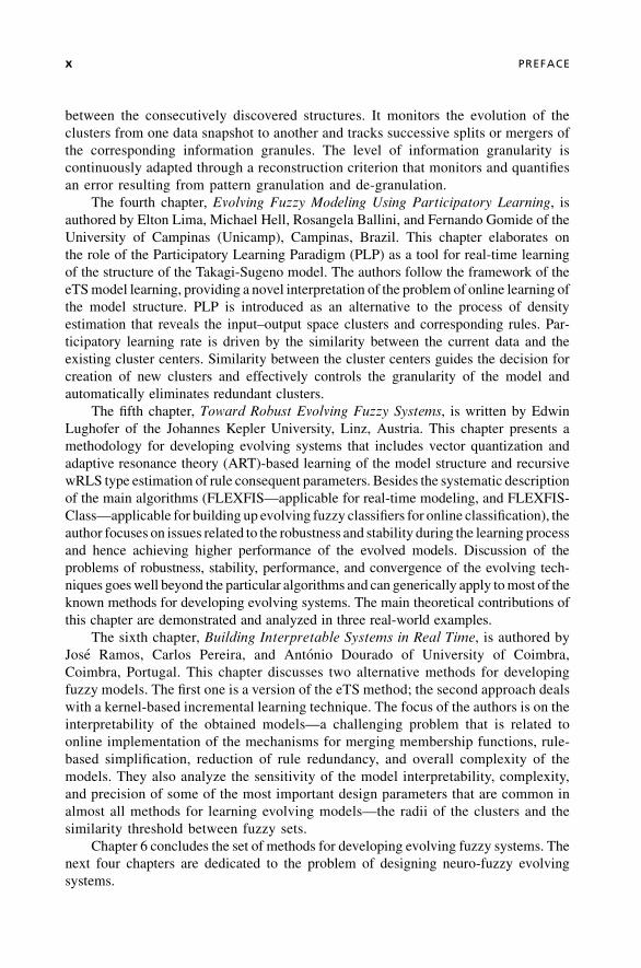
between the consecutively discovered structures. It monitors the evolution of the

clusters from one data snapshot to another and tracks successive splits or mergers of

the corresponding information granules. The level of information granularity is

continuously adapted through a reconstruction criterion that monitors and quantifies

an error resulting from pattern granulation and de-granulation.

The fourth chapter, Evolving Fuzzy Modeling Using Participatory Learning, is

authored by Elton Lima, Michael Hell, Rosangela Ballini, and Fernando Gomide of the

University of Campinas (Unicamp), Campinas, Brazil. This chapter elaborates on

the role of the Participatory Learning Paradigm (PLP) as a tool for real-time learning

of the structure of the Takagi-Sugeno model. The authors follow the framework of the

eTSmodel learning, providing a novel interpretation of the problem of online learning of

the model structure. PLP is introduced as an alternative to the process of density

estimation that reveals the input–output space clusters and corresponding rules. Par-

ticipatory learning rate is driven by the similarity between the current data and the

existing cluster centers. Similarity between the cluster centers guides the decision for

creation of new clusters and effectively controls the granularity of the model and

automatically eliminates redundant clusters.

The fifth chapter, Toward Robust Evolving Fuzzy Systems, is written by Edwin

Lughofer of the Johannes Kepler University, Linz, Austria. This chapter presents a

methodology for developing evolving systems that includes vector quantization and

adaptive resonance theory (ART)-based learning of the model structure and recursive

wRLS type estimation of rule consequent parameters. Besides the systematic description

of the main algorithms (FLEXFIS—applicable for real-time modeling, and FLEXFIS-

Class—applicable for building up evolving fuzzy classifiers for online classification), the

author focuses on issues related to the robustness and stability during the learning process

and hence achieving higher performance of the evolved models. Discussion of the

problems of robustness, stability, performance, and convergence of the evolving tech-

niques goeswell beyond the particular algorithms and can generically apply tomost of the

known methods for developing evolving systems. The main theoretical contributions of

this chapter are demonstrated and analyzed in three real-world examples.

The sixth chapter, Building Interpretable Systems in Real Time, is authored by

Jos�e Ramos, Carlos Pereira, and Antonio Dourado of University of Coimbra,

Coimbra, Portugal. This chapter discusses two alternative methods for developing

fuzzy models. The first one is a version of the eTS method; the second approach deals

with a kernel-based incremental learning technique. The focus of the authors is on the

interpretability of the obtained models—a challenging problem that is related to

online implementation of the mechanisms for merging membership functions, rule-

based simplification, reduction of rule redundancy, and overall complexity of the

models. They also analyze the sensitivity of the model interpretability, complexity,

and precision of some of the most important design parameters that are common in

almost all methods for learning evolving models—the radii of the clusters and the

similarity threshold between fuzzy sets.

Chapter 6 concludes the set of methods for developing evolving fuzzy systems. The

next four chapters are dedicated to the problem of designing neuro-fuzzy evolving

systems.

x PREFACE

Chapter 7, Online Feature Extraction for Evolving Intelligent Systems, is

authored by Seiichi Ozawa of Kobe University, Kobe, Japan, and S. Pang and Nikola

Kasabov of Auckland University of Technology, Auckland, New Zealand. This

chapter introduces an integrated approach to incremental (real-time) feature extrac-

tion and classification. The incremental feature extraction is done by two alternative

approaches. The first one is based on a modified version of the Independent Principle

Component Analysis (IPCA) method. It is accomplished through incremental eigen-

space augmentation and rotation, which are applied to every new training sample. The

second feature-extraction approach, called the Chunk IPCA, improves the compu-

tational efficiency of the ICPA by updating the eigenspace in chunks of grouped

training samples. The incremental feature-extraction phase is blended with an

incremental nearest-neighbor classifier that simultaneously implements classification

and learning. In a smart learning procedure, the misclassified samples are periodically

used to update the eigenspace model and the prototypes. The combination of feature

extraction, classification, and learning results forms an adaptive intelligent system

that can effectively handle online streams of multidimensional data sets.

Chapter 8, Stability Analysis for an Online Evolving Neuro-Fuzzy Recurrent

Network, is authored by Jos�e de Jesus Rubio of Autonoma Metropolitana University,

Azcapotzalco, Mexico. This chapter deals with an evolving neuro-fuzzy recurrent

network. It is based on the recursive creation of a neuro-fuzzy network by unsupervised

and supervised learning. The network uses a nearest-neighbor-type algorithm that is

combined with a density-based pruning strategy to incrementally learn the model

structure. Themodel structure learning is accompanied by anRLS-type learningmethod.

The chapter also includes a detailed analysis of the numeric stability and the performance

of the proposed evolving learning method.

The ninth chapter, Online Identification of Self-Organizing Fuzzy Neural Net-

works for Modeling Time-Varying Complex Systems, is authored by Girijesh Prasad,

Gang Leng, T. Martin McGinnity, and Damien Coyle of University of Ulster. The

focus of this chapter is on a hybrid fuzzy neural learning algorithm, in which a fuzzy

paradigm is used to enhance certain aspects of the neural network’s learning and

adaptation performance. The algorithm is exemplified by a self-organizing model,

called the Self-Organizing Fuzzy Neural Network (SOFNN), that possesses the

ability to self-organize its structure along with associated premise (antecedent)

parameters. The self-organizing neural network creates an interpretable hybrid neural

network model, making effective use of the learning ability of neural networks and

the interpretability of fuzzy systems. It combines a modified RLS algorithm for

estimating consequent parameters with a structure-learning algorithm that adapts the

network structure through a set of new ellipsoidal-basis function neurons. The result

of the proposed architecture and learning is a method that is computationally efficient

for online implementation.

Chapter 10, Data Fusion via Fission for the Analysis of Brain Death, is authored

by Ling Li, Y. Saito, David Looney, T. Tanaka, J. Cao, and Danilo Mandic of Imperial

College, London, UK, and addresses the problem of continuous analysis of time-

series signals, such as EEG, in order to detect an abnormal state such as brain death.

The chapter proposes that the signal is first decomposed into its oscillatory compo-

PREFACE xi

nents (fission) and then the components of interest are combined (fusion) in order to

detect the states of the brain.

The following three chapters are focused on themethodology for evolving clustering

and classification.

Chapter 11, Similarity Analysis and Knowledge Acquisition by Use of Evolving

Neural Models and Fuzzy Decision, is authored by Gancho Vachkov of Kagawa

University, Kagawa, Japan. This chapter presents an original evolving model for

real-time similarity analysis and granulation of data streams. Two unsupervised incre-

mental learning algorithms are proposed to compress and summarize the raw data into

information granules (neurons). This way, the original, raw data set is transformed into

the granulation (compressed) model and represented with a small number of neurons.

The author introduces two characteristic features—Center-of-Gravity Distance and

Weighted Average Size Difference—to adequately describe individual granules. The

similarity analysis is based on a fuzzy rule-based model that uses the two characteristic

features to analyze the similarity of the granulated data. The resulting computationally

effective algorithm can have numerous potential applications in problems that relate to

fast search through a large amount of images or sensory information, for proper data

sorting and classification.

Chapter 12, An Extended Version of the Gustafson-Kessel Algorithm for Evolving

Data Stream Clustering, is written by Dimitar Filev of Ford Research & Advanced

Engineering, Dearborn, Michigan, USA, and Olga Georgieva of Bulgarian Academy of

Sciences, Sofia, Bulgaria. The authors make the case for a new, evolving clustering

method, called the evolving GK-Like(eGKL) algorithm that resembles the Gustafson-

Kessel (GK) clustering algorithm as a general tool for identifying clusters with a generic

shape and orientation. The chapter discusses the methodology for recursive calculation

of the metrics used in the GK algorithm. It also introduces an original algorithm that is

characterized with adaptive, step-by-step identification of clusters that are similar to the

GK clusters. The algorithm is based on a new approach to the problem of estimation of

the number of clusters and their boundaries that is motivated by the identified similarities

between the concept of evolving clustering and the multivariate statistical process

control (SPC) techniques. The proposed algorithm addresses some of the basic problems

of the evolving systems field (e.g., recursive estimation of the cluster centers, inverse

covariance matrices, covariance determinants, Mahalanobis distance type of similarity

relations, etc.).

Chapter 13, Evolving Fuzzy Classification of Nonstationary Time Series, is by

Yevgeniy Bodyanskiy, Yevgeniy Gorshkov, Illya Kokshenev, and Vitaliy Kolodyazhniy

of the Kharkiv National University of Radio-Electronics, Kharkiv, Ukraine. The authors

present an evolving robust recursive fuzzy clustering algorithm that is based on

minimization of an original objective function of a special form, suitable for time-

series segmentation. Their approach is derived from the conjecture that the estimates that

are obtained from a quadratic objective function are optimal when the data belong to the

class of distributions with bounded variance. The proposed algorithm learns the cluster

centers and the corresponding membership functions incrementally without requiring

multiple iteration and/or initial estimate of the number of clusters. One of the main

advantages of this novel algorithm is its robustness to outliers. The algorithm can be

xii PREFACE

carried out in a batch or recursive mode and can be effectively used in multiple evolving

system applications (e.g., medical diagnostics and monitoring, data mining, fault

diagnostics, pattern recognition, etc.).

The second part of the book is comprised of four chapters discussing different

applications of EIS.

Chapter 14, Evolving Inferential Sensors in Chemical Process Industry, is

authored by Plamen Angelov of Lancaster University, Lancaster, UK, and Arthur

Kordon of the Dow Chemical Company, Freeport, Texas, USA. The chapter defines an

interesting and promising area of evolving system applications—design of inferential

sensors. Inferential (soft) sensors are widely used in a number of process-monitoring

and control applications as a model-based estimator of variables that are not directly

measured. While most of the conventional inferential sensors are based on first-

principle models, the concept of evolving systems offers the opportunity for online

adaptation of the models that are embedded in the inferential sensors when measured

data is made available. The authors provide a detailed discussion on the theory and the

state-of-the-art practices in this area—selection of input variables, preprocessing of

the measured data, addressing the complexity/accuracy dilemma, and so on. They

also justify the use in the inferential sensors of the Takagi-Sugeno model as a flexible

nonlinear mapping of multiple linear models. Further, they make the case for the eTS

as an effective approach for developing self-organizing and adaptive models as a

foundation of a new generation of highly efficient inferential sensors, called e-

Sensors. The idea of evolving inferential sensors is demonstrated in four case studies

from the chemical process industry.

Chapter 15, Recognition of Human Grasp by Fuzzy Modeling, is written by Rainer

Palm, Bourhane Kadmiry, and Boyko Iliev, of Orebro University, Orebro, Sweden. This

chapter provides another example of the potential of the evolving models for addressing

real-world practical problems—the evolving approach is applied to the problem of

modeling and quantification of human grasp in robotic applications. The authors analyze

three alternative algorithms for human grasp modeling and recognition. Two of those

algorithmsarebasedonevolvingTakagi-Sugenomodels that areused todescribe thefinger

joint angle trajectories (or fingertip trajectories) of grasp primitives,while the third one is a

hybrid of fuzzy clustering and hiddenMarkov models (HMM) for grasp recognition. The

authors experimentally prove out the advantages (recognition rate and minimal complex-

ity) of the first algorithm, employing an evolving TS model approximating the minimum

distance between the time clusters of the test grasp and a set of model grasps.

Chapter 16, Evolutionary Architecture for Lifelong Learning and Real-Time

Operation in Autonomous Robots, is by Richard J. Duro, Francisco Bellas, and

Jos�e Antonio Becerra of University of La Coruna, Spain. This chapter focuses on the

robotic applications of the evolving system concept. It discusses the fundamentals

of the evolvable architecture of a cognitive robot that exhibits autonomous adaptation

capability. The robot continuously adapts its models and corresponding controls

(behaviors) to the changing environment. The kernel of the robot intelligence is a

general cognitive mechanism that is associated with its multilevel Darwinist brain,

including short- and long-term memories and a unique Promoter-Based Genetic

Algorithm (PBGA) combining neural and genetic learning algorithms.

PREFACE xi i i

The final chapter, Applications of Evolving Intelligent Systems to Oil and Gas

Industry, is written by Jos�e JuanMac�ıas Hernandez of CEPSATenerife Oil Refinery and

University of La Laguna, Tenerife, Spain, and Plamen Angelov of Lancaster University,

Lancaster, UK. This chapter reviews the opportunities for application of evolving

systems to different process-control problems in oil refineries and in process industry

in general. Special attention is given to the evolving model-based industrial (indirect)

inferential sensors. The authors introduce an interesting e-Sensor version of the eTS

algorithm as an adaptive inferential sensor that is employed for product quality

monitoring. They also demonstrate how the Takagi-Sugeno modeling technique can

be expanded to the problem of automatic selection of a subset of important input

variables that are used to predict estimated process characteristics. Practical aspects of

the design and implementation of evolving inferential sensors, including initialization,

calibration, prediction, and performance under different operating modes, are also

presented.

To view supplemental material for this book, including additional software for

downloading, please visit http://www.lancaster.ac.uk/staff/angelov/Downloads.htm.

In closing, the editors would like to express their gratitude to all contributors and

reviewers for making this volume a reality. We hope that this book will be a useful tool

and inspiration for better understanding of the philosophy, theoretical foundations, and

potential of practical applications of the EIS.

The Editors,

Lancaster, UK

Dearborn, Michigan, USA

Auckland, New Zealand

February 2010

REFERENCES

Angelov, P. (2002).Evolving Rule-BasedModels: A Tool for Design of Flexible Adaptive Systems.

Heidelberg, New York, Springer-Verlag, ISBN 3-7908-1457-1.

Angelov, P., D. Filev (2004). “An Approach to On-line Identification of Takagi-Sugeno Fuzzy

Models.” IEEE Trans. on System, Man, and Cybernetics: Part B—Cybernetics, Vol. 34, No. 1,

pp. 484–498, ISSN 1094-6977.

Angelov, P., N. Kasabov (2006). “Evolving Intelligent Systems, eIS,” IEEE SMC eNewsLetter,

June 2006, pp. 1–13.

Angelov, P., X. Zhou (2006). “Evolving Fuzzy Systems from Data Streams in Real-Time.” Proc.

2006 International Symposium on Evolving Fuzzy Syst., Ambleside, UK, September 7–9,

2006, IEEE Press, pp. 29–35, ISBN 0-7803-9719-3.

Angelov, P., X. Zhou (2008). “On-Line Learning Fuzzy Rule-Based System Structure from Data

Streams.” Proc. World Congress on Computational Intelligence, WCCI-2008, Hong Kong,

June 1–6, 2008, IEEE Press, pp. 915–922, ISBN 978-1-4244-1821-3/08.

Astrom, K. J., B. Wittenmark (1989). Adaptive Control. Reading, MA: Addison-Wesley.

xiv PREFACE

Domingos, P., G. Hulten (2001). “Catching Up with the Data: Research Issues in Mining Data

Streams.” Workshop on Research Issues in Data Mining and Knowledge Discovery, Santa

Barbara, CA.

EC (2007). NMP-2008-3.2-2: Self-Learning Production Systems—Work Programme on Na-

nosciences, Nanotechnologies, Materials, and New Production Technologies. Available online

at ftp://ard.huji.ac.il/pub/251/NMP_Fiche_small__2008_02.pdf.

Fritzke, B. (1994). “Growing Cell structures: A Self-Organizing Network for Unsupervised and

Supervised Learning,” Neural Networks, Vol. 7, No. 9, pp. 1441–1460.

Hastie, T., R. Tibshirani, J. Friedman (2001). The Elements of Statistical Learning: Data Mining,

Inference and Prediction. Heidelberg, Germany: Springer-Verlag.

Kasabov, N. (1996). Foundations of Neural Networks, Fuzzy Systems and Knowledge Engineer-

ing. MIT Press.

Kasabov, N. (2002). Evolving Connectionist Systems: Methods and Applications in Bioinfor-

matics, Brain Study and Intelligent Machines. Springer-Verlag.

Kasabov, N. (2007). Evolving Connectionist Systems: The Knowledge Engineering Approach.

Springer-Verlag.

Kasabov, N., Q. Song (2002). “DENFIS: Dynamic Evolving Neural-Fuzzy Inference System and

Its Application for Time-Series Prediction.” IEEE Trans. on Fuzzy Systems, Vol. 10, No. 2, pp.

144–154.

Kordon, A. (2006). “Inferential Sensors as Potential Application Area of Intelligent Evolving

Systems.” International Symposium on Evolving Fuzzy Systems, EFS’06.

Lima, E., F. Gomide, R. Ballini (2006). “Participatory Evolving Fuzzy Modeling.” Proc. 2006

International Symposium on Evolving Fuzzy Systems EFS’06, IEEE Press, pp. 36–41, ISBN

0-7803-9718-5.

Ljung, L. (1988). System Identification: Theory for the User. Englewood Cliffs, NJ: Prentice-Hall.

Lughofer, E., P. Angelov, X. Zhou (2007). “Evolving Single- and Multi-Model Fuzzy Classifiers

with FLEXFIS-Class.” Proc. FUZZ-IEEE 2007, London, UK, pp. 363–368.

Macias-Hernandez, J. J., P. Angelov, X. Zhou (2007). “Soft Sensor for Predicting Crude Oil

Distillation Side Streams Using Takagi Sugeno Evolving Fuzzy Models.” Proc. 2007 IEEE

Intern. Conf. on Systems, Man, and Cybernetics, Montreal, Canada, pp. 3305–3310, ISBN 1-

4244-0991-8/07.

Pedrycz, W. (2005). Knowledge-Based Clustering: From Data to Information Granules. Chi-

chester, UK: Wiley-Interscience, pp. 316.

Wang, L., J. Mendel (1992). “Fuzzy Basis Functions, Universal Approximation and Orthogonal

Least-Squares Learning.” IEEE Trans. on Neural Networks, Vol. 3, No. 5, pp. 807–814.

Yager, R. (2006). “Learning Methods for Intelligent Evolving Systems.” Proc. 2006 Inter-

national Symposium on Evolving Fuzzy Systems EFS’06, IEEE Press, pp. 3–7, ISBN 0-

7803-9718-5.

Zadeh, L. A. (1975). “The Concept of a Linguistic Variable and Its Application to Approximate

Reasoning, Parts I, II and III,” Information Sciences, Vol. 8, pp. 199–249, 301–357; Vol. 9, pp.

43–80.

Zhou, X., P. Angelov (2007). “An Approach to Autonomous Self-Localization of a Mobile Robot

in Completely Unknown Environment Using Evolving Fuzzy Rule-Based Classifier.” First

2007 IEEE Intern. Conf. on Computational Intelligence Applications forDefense and Security,

Honolulu, Hawaii, USA, April 1-5, 2007, pp. 131–138.

PREFACE xv

1

LEARNING METHODS FOREVOLVING INTELLIGENT

SYSTEMSRonald R. Yager

Abstract: In this work we describe two instruments for introducing evolutionary

behavior into intelligent systems. The first is the hierarchical prioritized structure (HPS)

and the second is the participatory learning paradigm (PLP).

1.1 INTRODUCTION

The capacity to evolve and adapt to a changing environment is fundamental to human

and other living systems. Our understanding of the importance of this goes back to at

least Darwin [1]. As we begin building computational agents that try to emulate human

capacities we must also begin considering the issue of systems that evolve autono-

mously. Our focus here is on knowledge-based/intelligent systems. In these types of

systems, implementing evolution requires an ability to balance learning and changing

while still respecting the past accumulated knowledge. In this work we describe two

instruments for introducing evolutionary behavior into our intelligent systems. The first

is the hierarchical prioritized structure (HPS) and the second is the participatory

learning paradigm (PLP). The HPS provides a hierarchical framework for organizing

knowledge. Its hierarchical nature allows for an implicit prioritization of knowledge so

that evolution can be implemented by locating new knowledge in a higher place in the

Evolving Intelligent Systems: Methodology and Applications, Edited by Plamen Angelov, Dimitar P. Filev,

and Nikola Kasabov

Copyright � 2010 Institute of Electrical and Electronics Engineers

hierarchy. Two important aspects of the structure are considered in this work. The first

is the process of aggregating information provided at the different levels of the

hierarchy. This task is accomplished by the hierarchical updation operator. The other

aspect is the process of evolving the model as information indicating a change in the

environment is occurring.

The participatory learning paradigm provides a general learning paradigm that

emphasizes the role of what we already know in the learning process. Here, an attribute

about which we are learning is not viewed simply as a target being blindly pushed and

shoved by new observations but one that participates in determining the validity of the

new information.

Underlying both these instruments is a type of nonlinear aggregation operation that

is adjudicating between knowledge held at different levels. Central to this type of

aggregation is a process in which the privileged knowledge is deciding on the allowable

influence of the less-favored knowledge.

1.2 OVERVIEW OF THE HIERARCHICAL PRIORITIZED MODEL

In [2–5] we described an extension of fuzzy modeling technology called the hierar-

chical prioritized structure (HPS), which is based on a hierarchical representation of

the rules. As we shall subsequently see, this provides a rich framework for the

construction of evolving systems. The HPS provides a framework using a hierarchical

representation of knowledge in terms of fuzzy rules is equipped with machinery for

generating a system output given an input. In order to use this hierarchical framework

to make inferences, we needed to provide a new aggregation operator, called the

hierarchical updation (HEU) operator, to allow the passing of information between

different levels of the hierarchy. An important feature of the inference machinery of

the HPS is related to the implicit prioritization of the rules; the higher the rule is in the

HPS, the higher its priority. The effect of this is that we look for solutions in an ordered

way, starting at the top. Once an appropriate solution is found, we have no need to look

at the lower levels. This type of structure very naturally allows for the inclusion of

default rules, which can reside at the lowest levels of the structure. It also has an

inherent mechanism for evolving by adding levels above the information we want to

discard.

An important issue related to the use of theHPS structure is the learning of themodel

itself. This involves determination of the content of the rules as well the determination of

the level at which a rule shall appear. As in all knowledge-based systems, learning can

occur in many different ways. One extreme is that of being told the knowledge by some

(usually human) expert. At the other extreme is the situation in which we are provided

only with input–output observations and we must use these to generate the rules. Many

cases lie between these extremes.

Here we shall discuss one type of learning mechanism associated with the HPS

structure that lies between these two extremes, called the DELTA method. In this

we initialize the HPS with expert-provided default rules and then use input–output

2 LEARNING METHODS FOR EVOLVING INTELLIGENT SYSTEMS

observations to modify and adapt this initialization. Taking advantage of the HPS we are

able to introduce exceptions to more general rules by giving them a higher priority,

introducing them at a higher level in the hierarchy. These exceptions can be themselves

rules or specific points. This can be seen as a type of forgettingmechanism that can allow

the implementation of dynamic adaptive learning techniques that continuously evolve

the model.

1.3 THE HPS MODEL

In the following,wedescribe thebasic structure and the associated reasoningmechanismof

the fuzzy systemsmodeling framework called the hierarchical prioritized structure (HPS).

Assume we have a system we are modeling with inputs V and W and output U. At

each level of theHPS,we have a collection of fuzzy if-then rules. Thus for level j, we have

a collection of nj rules:

If V is Aji andW is Bji; thenU isDji i ¼ 1; . . . ; nj

We shall denote the collection of rules at the jth level asRj. Givenvalues for the input

variables, V¼ x� and W¼ y�, and applying the standard fuzzy inference to the rules at

level j, we can obtain a fuzzy subset Fj over the universe of U, where

FjðzÞ ¼ 1T

Xnji¼1

ljiDjiðzÞ with lji ¼ Ajiðx*Þ^Bjiðy*Þ and T ¼Xnji¼1

lji. Alternatively, we

can also calculateFjðzÞ ¼ Maxi½lji^DjiðzÞ�.We denote the application of the basic fuzzy

inference process with a given input, V¼ x� andW¼ y�, to this sub-rule base as Fj¼Rj .

Input.

In the HPS model, the output of level j is a combination of Fj and output of the

preceding level. We denote the output of the jth level of the HPS asGj. Gj is obtained by

combining the output the previous level, Gj�1, with Fj using the hierarchical updation

(HEU) aggregation operator subsequently to be defined. The output of the last level,Gn,

is the overall model output E. We initialize the process by assigning G0¼˘.

The key to inference mechanism in the HPS is the HEU aggregation operator

Gj¼ g(Gj�1, Fj), where

GjðzÞ ¼ Gj�1ðzÞþ ð1�aj�1ÞFjðzÞ

Here, aj�1¼Maxz[Gj�1(z)], the largest membership grade in Gj�1. See Figure 1.1.Let us look at the functioning of this operator. First we see that it is not pointwise in

that the value of Gj(z) depends, through the function aj�1, on the membership grade of

elements other than z. We also note that if aj�1¼ 1, no change occurs. More generally,

the largeraj�1 the less the effect of the current level. Thus, we see thataj�1 acts as a kindof choking function. In particular, if for some level j we obtain a situation in which Gj is

normal, and has an elementwithmembership grade one, the process of aggregation stops.

THE HPS MODEL 3

It is also clear thatGj�1 andFj are not treated symmetrically.We see that, as we get closer

to having some elements in Gj�1 with membership grade one, the process of adding

information slows. The form of the HEU essentially implements a prioritization of the

rules. The rules at the highest level of the hierarchy are explored first; if they find a good

solution, we look no further at the rules.

Figure 1.2 provides an alternative view of the HPS structure.

Input (V, W)

Output U

Level-1

Level-2

Level-n

Figure 1.1. Hierarchical prioritized structure.

HEU

F1

R1

HEU

F2

R2

HEU

Fn

Rn

G1 G2Gn–1

GnG0

Input

Figure 1.2. Alternative view of HPS.


1.4 AN EXAMPLE OF HPS MODELING

We shall illustrate the application of this structure with the following example

Example : Consider a functionW¼F(U, V) defined onU¼ [0,10] and V¼ [0,10].

Refer to Figure 1.3 for the following discussion. We shall assume that in the white areas

the value of the function is small and in the black areas the value of the function is large.

The figure could, for example, be representative of a geospatial mapping in which W is

the altitude and the black areas correspond to a mountain range.

We can describe this functional relationship by the following three-level HPS

structure:

Level-1: If U is close to five, then W is small. (Rule 1)

Level-2: If ððU�5Þ2þðV�5Þ2Þ0:5 is about two, thenW is large. (Rule 2)

Level-3: IfU and V are anything, thenW is small. (Rule 3)

For our purposes, we define the underlined fuzzy subsets as follows:

Small ¼ 0:3

5;0:6

6;1

7;0:6

8;0:3

9

� �and Large ¼ 0:3

21;0:6

22;1

23;0:6

24;0:3

25

� �

close to fiveðUÞ ¼ e�ðU�5Þ2

0:25and about fiveðrÞ ¼ e�ðr�2Þ

2

Let us look at three special cases.

1. U¼ 5 andV¼ 6. Here rule one fires to degree 1. Hence the output of the first level

is G1 ¼ 0:35; 0:6

6; 17; 0:6

8; 0:3

9

� �. Since this has maximal membership grade equal to

one, the output of the system is G1.

00

5

5

10

10

U

V

Figure 1.3. Structure of F(U, V).

AN EXAMPLE OF HPS MODELING 5

2. U¼ 6 and V¼ 6. Here the firing level of Rule 1 is 0.02 and the output of the first

level isG1 ¼ 0:25; 0:2

6; 0:2

7; 0:2

8; 0:2

9

� �and has maximal firing level 0.2. Applying the

input to Rule 2, we get a firing level of 1. Thus F2 ¼ 0:321; 0:622; 123; 0:624; 0:325

� �. Thus

G2ðzÞ ¼ 0:25; 0:2

6; 0:2

7; 0:2

8; 0:2

9; 0:24

21; 0:46

22; 0:823; 0:46

24; 0:24

25

� �and therefore a2¼ 0.8. Ap-

plying the input to Rule 3 three we get firing level 1. Thus

F2 ¼ 0:321; 0:622; 123; 0:624; 0:325

� �. Since G3(z)¼G2(z) þ (1� 0.8) F3(z) we get

G3 ¼ 0:265; 0:312

6; 0:4

7; 0:312

8;

�0:269; 0:24

21; 0:46

22; 0:823; 0:46

24; 0:24

25g.

Defuzzifying this value we get W¼ 16.3.

3. U¼ 9 and V¼ 8. In this case, the firing level of Rule 1 is 0; thus G1¼˘.

Similarly, the firing level of Rule 2 is also 0, and henceG1¼˘. The firing level of

Rule 3 is one, and hence the overall output is small.

1.5 HIERARCHICAL UPDATION OPERATOR

Let us look at some of the properties of this hierarchical updation operator g. IfA andB are

two fuzzy sets of Z, then we have g(A, B)¼D, where D(z)¼A(z) þ (1�a) B(z) witha¼Maxz2Z(A(z)). This operator is not pointwise as a depends on A(z) for all z2 Z. Thisoperator is a kind of disjunctive operator; we see that g(A,˘)¼A and g(˘, B)¼B. This

operator is not commutative g(A, B) 6¼ g(B, A). An important illustration of this is that

while g(Z, B)¼B, we have g(A, Z)¼D, where D(z)¼A(z) þ (1�a). The operator isalso nonmonotonic. Consider D¼ g(A, B) and D0 ¼ g(A0, B), where A�A0. Since

A(z)�A0(z) for all z, then a�a0. We have D0(z)¼A0(z) þ (1�a0) B(z) and D(z)¼A(z) þ (1�a) B(z). Since A�A0, monotonicity requires that D0(z)�D(z) for all z. To

investigate themonotonicity of g we look atD0(z)�D(z)¼A0(z)�A(z) þ B(z) (a�a0).Thus, while A0(z)�A(z)¼ 0, we have (a�a0)� 0, and therefore there is no

guarantee that D0(z)�D(z).

We can suggest a general class of operators that can serve as hierarchical aggregation

operators. Let T be any t-norm and S be any t-conorm [6]. A general class of hierarchical

updation operators can be defined as D¼HEU(A, B), where D(z)¼ S(A(z), T(1�a,B(z)) with a�Maxz(A(z)).

First, let us show that our original operator is a member of this class. Assume S is the

bounded sum, S(a, b)¼Min[1, a þ b] and T is the product, S(a, b)¼ ab. In this case,

D(z)¼Min[1, A(z) þ �aB(z)]. Consider the term A(z) þ �aB(z). Since a¼Maxz[A(z)],

then a¼A(z) and therefore A(z) þ �aB(z)�a þ (1�a) B(z)� 1. Thus D(z)¼A(z) þ (1�a) B(z), which was our original suggestion.

We can now obtain other forms for this HEU operator by selecting different S and T.

If S¼Max(_) and T¼Min(^), we getDðzÞ ¼ AðzÞ_ð�a^BðzÞÞ

If S is the algebraic sum, S(a, b)¼ a þ b� ab and T is the product, then

DðzÞ ¼ AðzÞþ �aBðzÞ��aAðzÞBðzÞ ¼ AðzÞþ �a�AðzÞBðzÞ


If we use S as the bounded sum and T as the Min, we get

DðzÞ ¼ Min½1;AðzÞþ �a^BðzÞ�

Since a�A(z), then A(z) þ �a ^ B(z)�a þ (1�a) ^ B(z)�a þ (1�a)� 1;

hence we get

DðzÞ ¼ AðzÞþ �a^BðzÞ

More generally, if S is the bounded sum and T is any t-norm, then

DðzÞ ¼ Min½1;AðzÞþ Tð�a^BðzÞÞ�

Since T(�a ^ B(z))� �a ¼ 1�A(z), then

DðzÞ ¼ AðzÞþ Tð�a;BðzÞÞ

1.6 THE DELTA METHOD OF HPS LEARNING

In the preceding, we have described the inference mechanism associated with

the hierarchical prioritized structure. We have said nothing about how we obtained the

rules in the model. The issue of the construction of the HPS model is an important

one. The format of the HPS model allows many different methods for obtaining the

model.

In this section we shall outline a dynamic learning approach for the construction

of an HPS that allows the system to continuously learn and evolve. We call this the

default-exception-learning-that’s-adaptive (DELTA) method for HPS. In this ap-

proach we initialize the HPS by providing a default representation of the relationship

we are trying to model. With this default relationship we allow the system builder to

provide an initial model of the system that will be augmented as we get more data about

the performance of the actual system. This default model can be as simple or as

complex as the designer’s knowledge of the system can support. In this approach the

augmentation of the model will be one in which we add specific observations and rules

to the HPS. The addition of knowledge to the structure will be driven by observations

that are exceptions to what we already believe the situation to be. The exceptions

will be captured and stored at the top level of the hierarchy. Groups of exceptions

shall be aggregated to form new rules, which will stored at the next level of the

hierarchy.

We shall use a three-levelHPSmodel as shown in Figure 1.4. For ease of explanation

we shall assume a model having a single input. The extension to multiple inputs is

straightforward.

The construction of the structure is initialized with the first and second levels being

empty. The third level is initializedwith our default information about the structure of the

relationship between the input and output variables V andU. In particular, the third level

THE DELTA METHOD OF HPS LEARNING 7

contains default rules of the form

If V is A thenU is f ðVÞ

In the above, f(V) is some prescribed functional relationship and A is a fuzzy

subset indicating the range of that default rule. The knowledge in the default can be any

manifestation of the prior expectation of the systemmodeler. It could be a simple rule that

saysU¼ b for all values ofV, a linear relationship that saysU¼ k1 þ k2V for all values of

V, or a collection of more complex rules based on some partitioning of the input space.

The HPS model will evolve based on observations presented to it, especially

observations that are exceptions towhatwe already believe. In particular, the information

in levels 1 and 2 will be obtained from the observations presented to the model. As we

shall see, level 1 will contain facts about individual observations that are exceptions to

what we already believe. Level 2 shall contain rules that aggregate these exceptions. The

aggregation process used here is very much in the spirit of the mountain clustering

method [7–10] introduced by Yager and Filev.

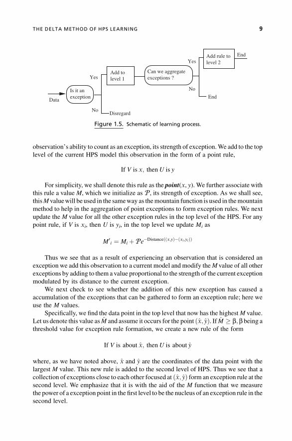
In Figure 1.5, we provide a flow diagram of the basic learning mechanism used in

this approach. In the following, we describe the basic mechanism for the construction of

this type of HPS. An observation (x, y) is presented to the HPS model. We calculate the

output for the input x, and denote this y�.We then compare this calculated outputwith the

desired output. If y and y� are close to each other, we can disregard this data and assume it

doesn’t provide any learning. If y and y� are not close, we use this data tomodify theHPS.

More specifically for the pair (y, y�) we calculate the valueClose(y, y�)2 [0,1] indicatingthe degree of closeness of the observed value and the calculated value. IfClose(y, y�)�a,a threshold level, we disregard the data. IfClose(y, y�) <a, we use this data to update themodel. We denote for this observation P ¼ 1�Close(y, y�) as a measure of this

Input U

Output V

Level 1: Exceptions

Level 2: Exception-Based Rules

Level 3: Default Rules

Figure 1.4. Exception-based hierarchy.


observation’s ability to count as an exception, its strength of exception.We add to the top

level of the current HPS model this observation in the form of a point rule,

If V is x; thenU is y

For simplicity, we shall denote this rule as the point(x, y). We further associate with

this rule a valueM, which we initialize as P, its strength of exception. As we shall see,

thisM valuewill be used in the sameway as themountain function is used in themountain

method to help in the aggregation of point exceptions to form exception rules. We next

update the M value for all the other exception rules in the top level of the HPS. For any

point rule, if V is xi, then U is yi, in the top level we update Mi as

M0i ¼ Mi þPe�Distanceððx;yÞ�ðxi ;yiÞÞ

Thus we see that as a result of experiencing an observation that is considered an

exception we add this observation to a current model and modify theM value of all other

exceptions by adding to them a value proportional to the strength of the current exception

modulated by its distance to the current exception.

We next check to see whether the addition of this new exception has caused a

accumulation of the exceptions that can be gathered to form an exception rule; here we

use the M values.

Specifically, we find the data point in the top level that now has the highestM value.

Let us denote this value as M and assume it occurs for the point ðx; yÞ. If M � b; b being athreshold value for exception rule formation, we create a new rule of the form

If V is about x; thenU is about y

where, as we have noted above, x and y are the coordinates of the data point with the

largest M value. This new rule is added to the second level of HPS. Thus we see that a

collection of exceptions close to each other focused at ðx; yÞ form an exception rule at the

second level. We emphasize that it is with the aid of the M function that we measure

the power of a exception point in the first level to be the nucleus of an exception rule in the

second level.

Data

Add to level 1

Can we aggregate exceptions ?

Add rule to level 2

End

Disregard

Is it an exception

Yes

No

End

Yes

No

Figure 1.5. Schematic of learning process.

THE DELTA METHOD OF HPS LEARNING 9

The final step is the cleansing and reduction of the top level by eliminating the

individual exception rules that are now accounted for by the formulation of this new rule

at the second level. We first modify our functionM at each point (x, y) in the top level to

form M0, where

M0ðx; yÞ ¼ Mðx; yÞ�Me�Distanceððx;yÞ�ðx;yÞÞ

We next eliminate all point rules for which M0(x, y)� 1�a.Further,we let A and B be the fuzzy subsets about x and y. For each exception point in

the top level, we calculate AðxiÞ and BðyiÞ and let ti¼Min (A(xi), B(yi)). We then

eliminate all exceptions for which ti� l, a threshold for exception cleansing.

It should be noted that the above procedure has a number of parameters affecting our

actions. In particular we introduced a, b, and l. It is with the aid of these parameters that

we are able to control the uniqueness of the learning process. For example, the smallerwe

make a, the more rigorous our requirements are for indicating an observation as an

exception; it is related to our sensitivity to exceptions. The parameter b determines

openness to the formulation of new rules. The choice of these parameters is verymuch in

the same spirit as choice of the learning rate used in the classical gradient learning

techniques such as back propagation. Experience with the use of this exception-based

machinerywill of course sharpen our knowledge of the effect of parameter selection. At a

deeper level the selection of these parameters should be based on how we desire the

learning to perform and gives us a degree of freedom in the design of our learning

mechanism, resulting, just as in the case of human learning, in highly individualized

learning.

It is important to emphasize some salient features of the DELTA mechanism for

constructing HPS models. We see this has an adaptive-type learning mechanism. We

initialize the system with current user knowledge and then modify this initializing

knowledge based on our observations. In particular, as with a human being, this has the

capability for continuously evolving. That is, even while it is being used to provide

outputs it can learn from its mistakes. Also we see that information enters the systems as

observations and moves its way down the system in rules very much in the way that

humans process information in the face of experience.

1.7 INTRODUCTION TO THE PARTICIPATORY LEARNINGPARADIGM

Participatory learning is a paradigm for computational learning systems whose basic

premise is that learning takes place in the framework of what is already learned and

believed. The implication of this is that every aspect of the learning process is effected

and guided by the learner’s current belief system. Participatory learning highlights

the fact that in learning we are in a situation in which the current knowledge of what we

are trying to learn participates in the process of learning about itself. This idea is

closely related to Quine’s idea of web of belief [11, 12]. The now-classic work by

Kuhn [13] describes related ideas in the framework of a scientific advancement.With the


participatory learning paradigm we are trying to bring to the field of computational

intelligence some important aspects of human learning. What is clear about human

learning is that it manifests a noncommutative aggregation of information; the order of

experiences and observations matters. Typically, the earlier information is more valued.

Participatory learning has the characteristic of protecting our belief structures fromwide

swings due to erroneous and anomalous observations while still allowing the learning of

new knowledge. Central to the participatory learning paradigm is the idea that observa-

tions conflicting with our current beliefs are generally discounted.

In Figure 1.6, we provide a partial systemic view of a prototypical participatory

learning process that highlights the enhanced role played by the current belief system.An

experience presented to the system is first sent to the acceptance or censor component.

This component, which is under the control of the current belief state, decides whether

the experience is compatible with the current state of belief; if it is deemed as

being compatible, the experience is passed along to the learning components, which

use this experience to update the current belief. If the experience is deemed as being too

incompatible, it is rejected and not used for learning. Thus we see that the acceptance

component acts as a kind of filler with respect to deciding which experiences are to

be used for learning. We emphasize here that the state of the current beliefs participates

in this filtering operation. We note that many learning paradigms do not include this

filtering mechanism; such systems let all data pass through to modify the current

belief state.

Because of the above structure, a central characteristic of the PLP (participatory

learning paradigm) is that an experience has the greatest impact in causing learning or

belief revision when it is compatible with our current belief system. In particular,

observations that conflict toomuchwith our current beliefs are discounted. The structure

of the participatory learning system (PLS) is such that it is most receptive to learning

when confronted with experiences that convey the message “What you know is correct

except for this little part.” The rate of learning using the PLP is optimized for situations in

which we are just trying to change a small part of our current belief system. On the other

hand, a PLS when confronted with an experience that says “You are all wrong; this is the

truth” responds by discounting what is being told to it. In its nature, it is a conservative

learning system and hence very stable. We can see that the participatory learning

environment uses sympathetic experiences tomodify itself. Unsympathetic observations

are discounted as being erroneous. Generally, a system based on the PLP uses the whole

context of an observation (experience) to judge something about the credibility of

the observation with respect to the learning agent’s beliefs; if it finds the whole

AcceptanceFunction

UpdationLearningProcess

Current Belief System

LearningExperience

Figure 1.6. Partial view of a prototypical participatory learning process.

INTRODUCTION TO THE PARTICIPATORY LEARNING PARADIGM 11

experience credible, it can modify its belief to accommodate any portion of the

experience in conflict with its belief. That is, if most of an experience or observation

is compatiblewith the learning agent’s current belief, the agent can use the portion of the

observation that deviates from its current belief to learn.

While the acceptance function in PLP acts to protect an agent from responding to

“bad” data, it has an associated downside. If the agent using a PLP has an incorrect belief

system about theworld, it allows this agent to remain in this state of blissful ignorance by

blocking out correct observations that may conflict with this erroneous belief model. In

Figure 1.7, we provide a more fully developed version of the participatory learning

paradigm that addresses this issue by introducing an arousal mechanism in the guise

of a critic.

The arousal mechanism is an autonomous component not under the control of the

current belief state. Its role is to observe theperformanceof the acceptance function. If too

many observations are rejected as being incompatible with the learning agent’s belief

model, this component arouses the agent to the fact that somethingmay bewrongwith its

currentstateofbelief;a lossofconfidenceis incurred.Theeffectof this lossofconfidenceis

to weaken the filtering aspect of the acceptance component and allow incoming experi-

ences that are not necessarily compatiblewith the current state of belief to be used to help

update thecurrentbelief.Thissituationcanresult inrapid learning in thecaseofachanging

environment once the agent has been aroused. Essentially, the role of the arousal

mechanism is to help the agent get out of a state of belief that is deemed as false.

Fundamentally, we see two collaborating mechanisms at play in this participatory

learning paradigm. The primary mechanism manifested by the acceptance function and

controlled by the current state of belief is a conservative one; it assumes the current state

of belief is substantially correct and requires only slight tuning. It rejects strongly

incompatible experiences and doesn’t allow them to modify its current belief. This

mechanism manifests its effect on each individual learning experience. The secondary

mechanism, controlled by the arousal mechanism, being less conservative, allows for the

possibility that the agent’s current state of belief may be wrong. This secondary

mechanism is generally kept dormant unless activated by being aroused by an accu-

mulation of input observations in conflict with the current belief. What must be

AcceptanceFunction

UpdationLearningProcess

Current Belief System

LearningExperience

ArousalMechanism

Figure 1.7. Fully developed prototypical participatory learning process.


emphasized is that the arousal mechanism contains no knowledge of the current beliefs;

all knowledge resides in the belief system. It is basically a scoring system calculating

how the current belief system is performing. It essentially does this by noting how often

the system has encountered incompatible observations. Its effect is not manifested by an

individual incompatible experience but by an accumulation of these.

1.8 A MODEL OF PARTICIPATORY LEARNING

As noted in the preceding, participatory learning provides a paradigm for constructing

computational learning systems; as such, it can used in many different learning

environments. In the following, we provide one example of a learning agent based on

the PLP to illustrate some instantiation of the ideas described above [14].While this is an

important example of learning in a quantitative environment, we note that the PLP can be

equally useful in the kind of symbolic learning environments found in the artificial

intelligence and machine learning community.

In the illustration of PL that follows, we have a context consisting of a collection of

variables, x(i), i¼ 1 to n. Here we are interested in learning the value of this collection of

variables. It is important to emphasize the multidimensionality of the environment in

which the agent is doing the learning.Multidimensionality, which is present inmost real-

world learning experiences, is crucial to the functioning of the participatory learning

paradigm since the acceptability of an experience is based on the compatibility of the

collection of observed values as awholewith the agent’s current belief. For simplicitywe

assume that the values of the x(i)2 [0,1]. The current state of the system’s belief consists

of a vector Vk�1, whose components Vk�1(i), i¼ 1 to n, consist of the agent’s current

belief about the values ofx(i). It is what the agent has learned after k� 1 observation. The

current observation consists of a vector Dk, whose components dk(i), i¼ 1 to n, are

observations about the variable x(i). Using a participatory learning type of mechanism,

the updation of our current belief is the vector Vk whose components are

VkðiÞ ¼ Vk�1ðiÞþarkð1�akÞðdkðiÞ�Vk�1ðiÞÞ ðIÞ

Using vector notation, we can express this as

Vk ¼ Vk�1þarkð1�akÞðDk�Vk�1Þ ðIbÞ

In the above,a2 [0,1] is a basic learning rate. The term rk is the compatibility of the

observation Dk with the current belief Vk�1. This is obtained as

rk ¼ 1� 1

n

Xni¼1jdkðiÞ�Vk�1ðiÞj

!

It is noted that rk2 [0,1]. The larger rk, the more compatible the observation is with the

current belief. One important feature that needs to be pointed out is the role that the

A MODEL OF PARTICIPATORY LEARNING 13

multidimensionality plays in the determination of the compatibility rk. The system is

essentially looking at the individual compatibilities as expressed by jdkðiÞ�Vk�1ðiÞj todetermine the overall compatibility rk. A particularly notable case is where for most of

the individual variables we have good compatibility between the observation and the

belief but a few are not in agreement. In this case, since there is a preponderance of

agreement we shall get a high value for rk and the system is open to learning. Here, then,

the system has received a piece of data that it feels is a reliable observation based on its

current belief and is therefore open to accept it and learn from the smaller part of the

observation, which is not what it believes. We shall call such observations kindred

observations. The agent’s openness to kindred observations plays an important part in

allowing PL-based systems to rapidly learn in an incremental fashion [15].

The term ak, also lying in the unit interval, is called the arousal rate. This is obtained

by processing the compatibility using the formula

ak ¼ ð1�bÞak�1þ bð1�rkÞ ðIIÞ

Here b2 [0,1] is a learning rate. As pointed out in [14], b is generally less than a. We see

that ak is essentially an estimate of the negation, one minus, the compatibility. Here we

note that a low arousal rate, small values for ak, is an indication of a good correspondence

between the agent’s belief and the external environment. In this case, the agent has

confidence in the correctness of its belief system. On the other hand, a value for ak closer

to one arouses the agent to the fact that there appears to be some inconsistency between

what it believes and the external environment.

We see from equation (Ib) that when ak� 0, the learning from the current

observation Dk is strongly modulated by rk, the compatibility of Dk with the current

belief Vk�1. If the compatibility rk is high, we learn at a rate close to a; if the

compatibility rk is low, we do not learn from the current observation. On the other

hand, when ak� 1, and therefore the agent is concerned about the correctness of its

belief, the term rkð1�akÞ�1 is independent of the value rk and hence the agent is not

restrained by its current belief from looking at all observations.

We note that the updation algorithm (I) is closely related to the classicWidrow-Hoff

learning rule [16].

VkðiÞ ¼ Vk�1ðiÞþaðdkðiÞ�Vk�1ðiÞÞ ðW-HÞ

The basic difference between (I) and (W-H) is the inclusion of the term arkð1�akÞinstead of simple a. This results in a fundamental distinction between the classic leaning

model (W-H) and the PL version. In the classic case, the learning ratea is generallymade

small in order to keep the system from radically responding to erroneous or outlier

observations. In the PL version, the basic learning rate a can be made large because the

effect of any observation incompatible with the current belief is repressed by the term

rkð1�akÞ when ak is small. This effectively means that in these PL systems, if a relatively

good model of the external environment is obtained, the system can very rapidly tune

itself and converge. On the other hand, the classic model has a much slower rate of

convergence.


An often-used strategy when using the classic learning algorithm (I) is to let a be a

function of the number of observations k. In particular, one lets a be large for low values

of k and then lets it be smaller as k increases. In the PLP, it would seem that here we

should treat the learning parameter b in a similar manner.

Whatwe emphasize here is thatwe determined the acceptability of an observation by

using the pointwise compatibilities of the features of the observation with the agent’s

current belief about the values of the features. More complex formulations for the

determination of acceptability can be used within the PLP. For example, in many real

learning situations the internal consistency of the features associatedwith an observation

(experience) plays a crucial role in determining the credibility of an observation. The

knowledge of what constitutes internal consistency, of course, resides in the current

belief systems of the learning agent.When a person tells us a story about some experience

he had, a crucial role in our determining whether to believe him is played by our

determination of the internal consistency of the story.At amore formal level, in situations

in which we are trying to learn functional forms from data, it would appear that the

internal consistency of the data in the observation could help in judging whether an

observation should be used for learning.

1.9 INCLUDING CREDIBILITY OF THE LEARNING SOURCE

Letusconsider thenatureofa learningexperience.Generally, a learningexperiencecanbe

seen to consist of two components.Thefirst is the content of the experience;wehave been

dealing with this in the preceding. The second is the source of the content. Information

about both these components is contained in the agent’s current belief system.

In order to decide on the degree of acceptability of a learning experience and its

subsequent role in updating the current belief, a participating learning-based systemmust

determine two quantities. The first is the compatibility of the content of the experience

with the system’s current belief system. The second is the credibility of the source. The

information needed to perform these calculations is contained in the agent’s current

belief system. A point we want to emphasize is that information about the source

credibility is also part of the belief structure of a PL agent in a similar way as information

about the content. That is, the concept of credibility of source is essentially a measure of

the congruency of the current observation’s source with the agent’s belief of what are

good sources.

Generally, compatible content is allowed into the system and is more valued if it is

from a credible source rather than a noncredible source. Incompatible content is

generally blocked, and more strongly blocked from a noncredible source than from a

credible source.

As we have pointed out, a learning experience consists of content as well as an

indication of its source.Wenoted that the credibility of the source should play a role in the

learning process. In the model previously presented we paid no attention to the source.

We were implicitly assuming that the source had complete credibility. Let us now

consider including information about the source credibility in our learning model based

on the participatory learning paradigm.

INCLUDING CREDIBILITY OF THE LEARNING SOURCE 15

Here we shall begin to look at ways of including source credibility in the learning

process.Weassumewehaveacollectionofpossiblesourcesofcontent,S¼ {S1,. . .,Sn}. Inthis situation, we associate with each source a value C(j)2 [0,1] indicating the agent’s

current belief about the credibility of content provided by source Sj. This information is

stored in thebelief systemof theagent doing the learning.Wecandenote this as avectorC.

Consider that now we are in a situation in which the kth observation is provided by

source Sj. We now provide a form for our updation algorithm (I) that takes into account

the learner’s perceived credibility of this source, C(j). Here

Vk ¼ Vk�1þa CðjÞrkð1�akÞðdkðiÞ�Vk�1ðiÞÞ ðIcÞ

We see that a source with zero credibility has no effect, Vk ¼ Vk�1. On the other hand, inthe case when C(j)¼ 1, we get our original model.

The process of updating the arousal, aK, associatedwith themodel is also affected by

the credibility of the source. In these cases, we must modify (II) to take into account

the credibility of the source. We first note that the original arousal-level updation

algorithm was

ak ¼ ð1�bÞak�1þ bð1�rkÞ

or equivalently

ak ¼ ak�1þ bð�rk�ak�1Þ

where

�rk ¼ 1�rk

Modifying this to take into account the credibility of the source, we get

ak ¼ ak�1þCðjÞbð�rk�ak�1Þ ðIIcÞ

Again we see that sources with zero credibility do not affect our degree of arousal; on the

other hand, for those with credibility one, we get the original model.

We note that formula (IIc) can be expressed as

ak ¼ ð1�CðjÞbÞak�1þCðjÞb�rkImplicit in our inclusion of the credibility of the sources has been an assumption that

a source’s credibility,C(j), is fixed.More generally, the agent using the PLPwill learn and

update its belief about the credibility of the sources as a result of its learning experiences

in a manner similar to theway it learns content. Before providing this generalization, we

shall more usefully denote the credibility of source Sj as Ck(j), indicating the credibility

of Sj after the kth learning experience.

In the following, we shall provide a formula to allow the updation of the source

credibility. In expressing this formulation we shall find it convenient to use the termMjk


defined such thatMjk¼ 1 if Sj is the source of the kth observation, andMjk¼ 0 if Sj is not

the source of the kth experience. Using this notation we express our algorithm for

modifying the source credibility as

CkðjÞ ¼ Ck�1ðjÞþMjkl�ak�1ðrk�Ck�1Þ ðIIIÞ

where �ak�1 ¼ 1�ak�1 and l2 [0,1] is a base learning rate. We note that if Sj is not the

source of the kth learning experience, thenMjk¼ 0 andCk(j)¼Ck�1(j). Thus, in this casewe do not make any changes in our credibility. If Mjk¼ 1, then

CkðjÞ ¼ Ck�1ðjÞþ l�ak�1ðrk�Ck�1ðjÞÞ ¼ ð1�l�ak�1ÞCk�1ðjÞþ l�ak�1Þrk

Here we see l�ak�1 is an effective learning rate; it is the product of our base learning rateand the negation of the arousal level. Essentially �ak�1 is the confidence in the current

model. Thus, if �ak�1 ¼ 1, thenCkðjÞ ¼ Ck�1ðjÞþ l�ak�1ðrk�Ck�1ðjÞÞ. Here rK is beingused to calculate the current degree of performance of the source.

We make some observations about the learning-updation model for the Ck(j), First,

we note that if there exists only one source S¼ {S1}, thenwewill getCk(1)¼ 1� ak. That

is, the credibility of the agent is the negation of the arousal level. Since 1� aK is

essentially the credibility of themodel, we see that the credibility of a sole source and the

credibility of the resulting model are equivalent.

We note that in the source credibility updation algorithm (III) we can have different

base learning rates for each source. Thus we can have l(j) instead of l, where l(j) is thebase rate of learning the credibility of the jth agent. Further, if l(j)¼ 0, then Ck(j)¼Ck�1(j) for all k. This implies a fixed assigned credibility for the jth source.

1.10 TYPES OF LEARNING SOURCES

In the following, we shall try to identify and classify some types of sources of content

that are involved in learning experiences. The first type of source is direct sensory

experiences. These are related to observations we make with our own sensory organs.

Examples of this are seeing an auto accident, being at a baseball game and watching

the Yankees win, smelling alcohol on somebody’s breath, or hearing John tell Mary

“I love you.”

The second type we shall denote as an authority. Examples of learning experiences

from an authority are being told something by another person, reading something in a

book or obtaining it from the Internet, and hearing news on the radio or seeing it on TV.

The basic idea is that the contents have been processed by some other cognitive agent. For

these types of sources the content can be subject to “interpretation” by the processing

agent.

A third source of content is electromechanical sensor data. This is data obtained

through some electromechanical device such as the speedometer on your car, a ther-

mometer,or the typesofscreensair trafficcontrollersuse.Numerousother typesofdevices

can be listed. Here the contents have been processed by a neutral physical device.

TYPES OF LEARNING SOURCES 17

Another source of content is what we shall call reflection. Here we mean the

conscious rational manipulation of information already in an agent’s belief system that

brings to the agent’s awareness knowledge that is implicit in the current belief system.

Deduction, induction, and reasoning are examples of this source. It can be seen as a

kind of reorganization of knowledge in the agent’s belief system. An interesting

example occurs when the agent becomes aware of a conflict in his system. This source

of content here is clearly distinct from the preceding three in that in the first three the

source of the new content comes from outside the agent. In the case of reflection, the

source of the content is internal to the agent. An additional aspect of what we have in

mind with this reflective source of information that we want to emphasize without

getting too deep into philosophical issues is the conscious rational aspect of this

process.

Another source of content for our learning experiences is what we shall denote as

mystic. Examples of this would be information coming from the subconscious, dreams,

hallucinations, being told by God, and what some people call gut feeling. What we want

to point out here is that for the most part this can be considered as internally sourced

information; however, for some of these, such as being told byGod, it is not clearwhether

it is from external or internal sources. Further, for some people, this type of content can

be considered as “empty.” However, for others, this is a valid type of learning experience.

This category of learning is becoming an increasingly important one in our time since one

objective of many security systems is to try to understand, predict, and manipulate the

actions of terrorists, many of whom are religious fundamentalists who construct their

belief system using this type of source.

We feel that various types of agents can be modeled by formalizing the credibility

that they attach to these different categories of sources of learning experiences.

1.11 CONCLUSION

In this work we described two instruments for introducing evolutionary behavior into

intelligent systems. The first was the hierarchical prioritized structure (HPS) and the

second was the participatory learning paradigm (PLP). We saw that underlying both

these instruments is a type of nonlinear aggregation operation that is adjudicating

between knowledge held at different levels. Central to this type of aggregation is a

process in which the privileged knowledge is deciding on the allowable influence of the

less-favored knowledge.

1.12 REFERENCES

1. Darwin, C., The Origin of the Species, London, 1859.

2. Yager, R. R., “On a Hierarchical Structure for Fuzzy Modeling and Control.” IEEE Trans. on

Systems, Man and Cybernetics 23, 1189–1197, 1993.

3. Yager, R. R., “On the Construction of Hierarchical Fuzzy Systems Models.” IEEE Trans. on

Systems, Man and Cybernetics Part C: Applications and Reviews 28, 55–66, 1998.


4. Rozich, R., T. Ioerger, R. R., Yager, “FURL—ATheory RevisionApproach to Learning Fuzzy

Rules.” IEEE World Congress on Computational Intelligence, Honolulu, Hawaii: Proceed-

ings of Conference on Fuzzy Systems, 791–796, 2002.

5. Yager, R. R., “Organizing Information Using a Hierarchical Fuzzy Model.” In Systematic

Organisation of Information in Fuzzy Systems ( P., Melo-Pinto, H., Teodrescu, T., Fukuda,

eds.), NATO Science Series. IOS Press: Amsterdam, 2003, pp. 53–69.

6. Klement, E. P., R. Mesiar, E., Pap, Triangular Norms. Dordrecht, Kluwer Academic Publish-

ers, 2000.

7. Yager, R. R., D. P., Filev, “Approximate Clustering via theMountainMethod.” IEEETrans. on

Systems, Man and Cybernetics 24, 1279–1284, 1994.

8. Yager, R. R., D. P., Filev, “Generation of Fuzzy Rules by Mountain Clustering,” Journal of

Intelligent and Fuzzy Systems 2, 1994, pp. 209–219.

9. Rickard, J. T., R. R. Yager, W., Miller, “Mountain Clustering on Non-uniform Grids Using

p-Trees,” Fuzzy Optimization and Decision Making 4, 2005, pp. 87–102.

10. Yager, R. R., D. P., Filev, “Summarizing Data Using a Similarity-Based Mountain Method,”

Information Sciences 178, 2008, pp. 816–826.

11. Quine, M.V.O., “Two Dogmas of Empiricism,” Philosophical Review 60, 1951, pp. 20–43.

12. Quine, M. V. O., From a Logical Point of View. Cambridge: Harvard Press, 1953.

13. Kuhn, T. S., The Structure of Scientific Revolutions. University of Chicago Press: 1962.

14. Yager, R. R., “A Model of Participatory Learning.” IEEE Trans. on Systems, Man and

Cybernetics 20, 1990, pp. 1229–1234.

15. Yager, R. R., D. Z., Zhang, “Effective Suggestion Based on Participatory Learning,” Expert

Systems: Research & Applications 7, 1994, pp. 423–432.

16. Widrow, B., M. E., Hoff, “Adaptive Switching Circuits,” IRE Western Electric Show and

Convention Record, Part 4, 1960, pp. 96–104.

REFERENCES 19

2

EVOLVING TAKAGI-SUGENOFUZZY SYSTEMS FROM

STREAMING DATA (eTSþ )Plamen Angelov

2.1 BACKGROUND AND MOTIVATION

It is a well-known fact that nowadays we are faced not only with large data sets that we

need to process quickly, but with huge data streams (Domingos &Hulten, 2001). Special

requirements are also placed by the fast-growing sector of autonomous systems, where

systems that can retrain and adapt on-the-fly are needed (Patchett&Sastri, 2007). Similar

requirements are enforced by the advanced process industries for self-developing and

self-maintaining sensors (Qin et al., 1997). Now, they even talk about self-learning

industries (EC, 2007). All of these requirements cannot be met by using offline

methods and systems that can merely adjust their parameters and are linear (Astrom

&Wittenmark, 1989). These requirements call for a new type of system that assumes the

structure of nonlinear, nonstationary systems to be adaptive and flexible.

The author of this chapter started research work in this direction around the turn of

the century (Angelov, 2002; Angelov & Buswell, 2001), and this research culminated in

proposing with Dr. D. Filev the so-called evolving Takagi-Sugeno (eTS) fuzzy system

(Angelov&Filev, 2003). Since then, a number of improvements of the original algorithm

have been made, which require a systematic description in one publication. In this

chapter an enhanced version of the eTS algorithm will be described, which is called


and Nikola Kasabov


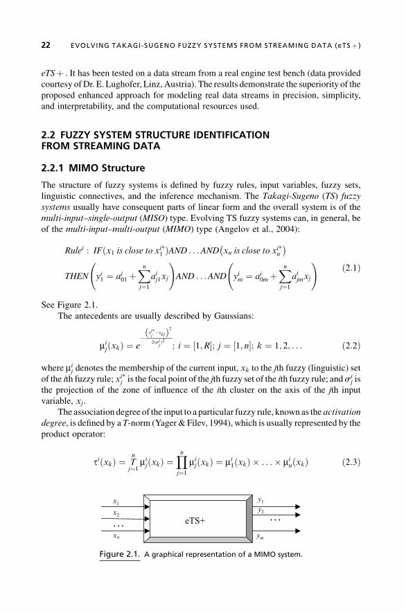
eTSþ . It has been tested on a data stream from a real engine test bench (data provided

courtesy ofDr. E. Lughofer, Linz, Austria). The results demonstrate the superiority of the

proposed enhanced approach for modeling real data streams in precision, simplicity,

and interpretability, and the computational resources used.

2.2 FUZZY SYSTEM STRUCTURE IDENTIFICATIONFROM STREAMING DATA

2.2.1 MIMO Structure

The structure of fuzzy systems is defined by fuzzy rules, input variables, fuzzy sets,

linguistic connectives, and the inference mechanism. The Takagi-Sugeno (TS) fuzzy

systems usually have consequent parts of linear form and the overall system is of the

multi-input–single-output (MISO) type. Evolving TS fuzzy systems can, in general, be

of the multi-input–multi-output (MIMO) type (Angelov et al., 2004):

Rulei : IFðx1 is close to xi*1 ÞAND . . .AND xn is close to xi*n

� �THEN yi1 ¼ ai01þ

Xnj¼1

aij1xj

!AND . . .AND yim ¼ ai0mþ

Xnj¼1

aijmxj

! ð2:1Þ

See Figure 2.1.

The antecedents are usually described by Gaussians:

mijðxkÞ ¼ e

�xi*j�xkjð Þ2

2ðsijÞ2

; i ¼ 1;R½ �; j ¼ 1; n½ �; k ¼ 1; 2; . . . ð2:2Þ

where mij denotes the membership of the current input, xk to the jth fuzzy (linguistic) set

of the ith fuzzy rule; xi*j is the focal point of the jth fuzzy set of the ith fuzzy rule; andsij is

the projection of the zone of influence of the ith cluster on the axis of the jth input

variable, xj .

The association degree of the input to a particular fuzzy rule, known as the activation

degree, is defined by a T-norm (Yager & Filev, 1994), which is usually represented by the

product operator:

tiðxkÞ ¼ Tn

j¼1mijðxkÞ ¼

Ynj¼1

mijðxkÞ ¼ mi

1ðxkÞ . . . minðxkÞ ð2:3Þ

eTS+ ……

x1

x2

xn

y1

y2

ym

Figure 2.1. A graphical representation of a MIMO system.

22 EVOLVING TAKAGI-SUGENO FUZZY SYSTEMS FROM STREAMING DATA (eTS þ )

Each fuzzy rule approximates the output in a local region centered at the focal point

and defined in a fuzzy way (the degree of truth and influence of this local approximation

depends on the distance to the focal point and is represented by the membership

function (2.2)). Thanks to the fuzzily defined antecedents, any nonlinear system can

be approximated by a set of fuzzily coupled locally linear subsystems (Wang &

Mendel, 1992).

2.2.2 Neural Network Implementation of eTSþIt is well known that the TS fuzzy system can be represented as a neural network

(Jang, 1993). The network-like structure enables the flexibility and parallelism and the

development of effective learning techniques. The confluence of neural networks as

structure frameworkwith the power of fuzzy systems as knowledge granulemodels leads

to neuro-fuzzy constructs. eTSþ can also be represented as a six-layer neuro-fuzzy

system (Figure 2.2), which is similar to the fuzzy basis-function networks (Wang &

Mendel, 1992).

The first layer takes the inputs,xk and feeds the second layer, which has neuronswith

activation functions determined by the membership functions mijðxkÞ defined in (2.2).

In this way, the second layer acts as the granulation of the input universes. The third layer

xn

xn

x1

x1

AND

AND

N

N

xn

x1

*11

*11 ,x

*1*1 , nnx

*1

*1 , RRx

**, Rn

Rnx

Layer 1 Inputs

Layer 2 Fuzzy Sets

Layer 3 Aggregation

Layer 4 Normalization

Layer 5 Consequents

Layer 6 Outputs

a11 an1

a01

11

1n

R1

Rn

1

R

a0R

a1R

anR

1

R

1

R

Rmy

11y

1y

my

Ry1

1my

Figure 2.2. eTSþ as a neural network.

FUZZY SYSTEM STRUCTURE IDENTIFICATION FROM STREAMING DATA 23

of the network aggregates the degrees of satisfaction of particular fuzzy sets per input

variable and performs the T-norm (usually product operation). It gives as output

the degree of activation of each particular fuzzy rule tiðxkÞ defined in (2.3). Further,

in layer 4, the activation levels are normalized in order of the contributions of the rules to

the overall output to sum up to 1 (or 100%). The first four layers represent the antecedent

part of the fuzzy system. The remaining layers, 5 and 6, are responsible for the

consequent part, and they are therefore linked to the antecedent part through links from

layer 1 in order to feed the inputs into layer 5 (bold lines in Figure 2.2). This layer also

gets parameter values andmultiplies them by the inputs to produce the local output of the

linear subsystem. Finally, layer 6 sums together the local outputs by first cross-

multiplying each one of them by the normalized activation level, liðxkÞ, and produces

the m outputs.

2.2.3 Unsupervised Learning Antecedents by Recursive DensityEstimation

Historically, first came the assumption that the structure of the fuzzy systems is defined

a priori based entirely on expert knowledge (Zadeh, 1975). Later, it was demonstrated

that the structure can be developed based on partitioning the entire data space into axes-

orthogonal hyper-boxes along the linguistic variables and assigning membership

functions to each box (Sugeno & Kang, 1988). Methods for automatic fuzzy systems

design (e.g. using genetic algorithms) were also developed (Angelov & Buswell, 2002;

Roubos et al., 2003). However, all these methods are applicable for batch, offline modes

of providing the data. For the casewhen the data are streaming, novel online methods for

fuzzy system structure identification are required. One effective online technique

proposed in Angelov and Filev (2003) is based on partitioning the data space into

overlapping local regions through recursive density estimation (RDE) and associating

clusters (respectively fuzzy sets) to them.

The density of the data space can be estimated by the mountain function (Yager &

Filev, 1994):

MðvÞ ¼XKi¼1

e� v�zij j2

2s2 ð2:4Þ

where v denotes the centre of a grid; zi is the current data point (for the purpose of fuzzy

system identification z is considered to be an input/output pair, z¼ [xT,yT]T; s is the

radius of the cluster; and K is the number of data points.

This concept borrows from the Parzen windows (Hastie et al., 2001) and Gaussian

kernel-based estimators, KDE (Elgammal et al., 2002). It is taken further in the

subtractive clustering (Chiu, 1994) where the need of the grid is replaced by using

each data point as a prototype of a cluster focal point. An alternative clustering method

that was also used for data space partitioning aiming at fuzzy systems design is

participatory learning (Silva et al., 2005). All of the above methods, however, rely on

the use of thresholds to decide whether a new cluster should be formed. eClustering,

proposed in Angelov (2004), is a principally different approach in that it applies to


streaming data and is one-pass (noniterative), and in its current version, called

eClusteringþ , it does not rely on user- or problem-specific thresholds. It estimates

the density at a data point using a Cauchy function:

DtðztÞ ¼ 1

1þ 1

t�1Xt�1i¼1

Xnþm

j¼1ðztj�zijÞ2

D1ðz1Þ ¼ 1; t ¼ 2; 3; . . .

ð2:5Þ

where DtðztÞ is the density of the data evaluated around the last data point of the data

stream provided to the algorithm zt; n denotes the dimension of the inputs vector;m is the

dimension of the outputs vector; and t denotes the number of points for which

information about z is available.

In eClustering the density,DtðztÞ is evaluated recursively and thewhole information

that concerns the spatial distribution of all data is accumulated in a small number

(n þ m þ 1) of variables (bt and ctj; j ¼ ½1; nþm�):

DtðztÞ ¼ t�1

t�1ð ÞXnþm

j¼1z2tj þ 1

!þ bt�2

Xnþm

j¼1ztjctj

D1ðz1Þ ¼ 1; t ¼ 2; 3; . . .

ð2:6Þ

where bt ¼ bt�1þXnþm

j¼1z2ðt�1Þj; b1 ¼ 0; ctj ¼ cðt�1Þj þ zðt�1Þj; and c1j ¼ 0.

Note that while t can grow large, both n andm are usually small and finite numbers.

The recursive density estimator (RDE) (2.6) has broader application areas than

online evolving fuzzy clustering and fuzzy systems design. In Angelov et al. (2008a) it

was applied for detecting novelties in video streams. RDE proved to work faster than the

well-established KDE approach by an order of magnitude. In Angelov et al. (2008c),

RDEwas used to generate a passivemethod for collision avoidance in uninhabited aerial

systems. Both applications are very important for the emerging market of autonomous

and robotic systems.

RDE is the cornerstone component of eClusteringþ (which itself is used for the

online design of eTSþ ). RDEprovides a computationally efficient technique to estimate

online in one-pass the generalization capability and the representativeness of a particular

data point. Obviously, data points with high density are good candidates to be cluster

focal points (respectively, focal points of antecedents of fuzzy rules). If a data point is

selected to be a cluster focal point, its density determined at themoment when it becomes

a focal point by equation (2.6) will be kept in memory and updated. The update is

necessary due to the online nature of the algorithm and because any new data point

coming from the data streamwill influence the data density (seen in the summation over i

in equation (2.5)). The density around cluster focal points can also be recursively updated


(Angelov, 2004) by:

Dtðzi*Þ ¼ t�1

t�1þðt�2Þ 1Dt�1ðzi*Þ �1�

þXnþm

j¼1ðztj�zðt�1ÞjÞ

;

D1ðzi*Þ ¼ 1; t ¼ 2; 3; . . . ð2:7Þ

where i� denotes the focal points of the ith fuzzy rule.

The aim of the data space partitioning used in fuzzy systems design, however, differs

from the aim of the conventional clustering (Duda et al., 2000). The latter aims to find

natural groupings in such a way that the data points in a certain cluster are compact and

clusters are well separable. When data space partitioning is used for the purpose of

forming a fuzzy rule base, the clusters normally overlap and are not necessarily mutually

exclusive. Therefore, the second objective (well-separable clusters) is not so important

when the partitioning is used for the design of a fuzzy system. In this case, the aims of data

space partitioning can be formulated as.

. Form representative clusters with high generalization capability.

. Coverage—ensure that themembership functions of the fuzzy sets that are formed

around cluster focal points cover the entire data space.

. Determine the number of clusters from data distribution alone.

. Avoid user- and problem-specific thresholds.

. Simplify the structure by removing least representative clusters as the data pattern

evolves.

The first aim is achieved by selecting the data points with the highest value ofD. The

second aim is formally satisfied if the membership functions are of Gaussian type.

In practice, however, the values of the membership functions outside the so-called

2s zone (Hastie et al., 2001) are negligibly small. Let us denote the number of outer data

points (points that do not lie inside the 2s zone of any of the clusters) at the tth time

instant (after t data samples are read) by Nt. That is:

Nt Ntþ 1; zijt�zi*j > 2si

jt for 8i ¼ ½1;R� and 8j ¼ ½1; nþm� ð2:8Þ

The first aim of the data space partitioning as described above (forming represen-

tative clusters) can be achieved by forming clusters around focal points that have high

density,

Condition A1: hDtðztÞ > maxR

i¼1Dtðzi*t Þ;h ¼

1 mij xtð Þ > e�2; 8i; 8j

Nt�3log t

otherwise

8<: ; t ¼ 2; 3; . . .

whereh is the normalized number of “outer” points (Figure 2.3); obviously, the higherh,the easier it is to create a new cluster.


Note that the factor h plays a role only after several (at least 5) outer points. In

Angelov et al. (2004b), an alternative form of Condition A was proposed:

Condition A2 : DtðztÞ > maxR

i¼1Dtðzi*t Þ OR DtðztÞ < min

R

i¼1Dtðzi*t Þ

ConditionA2 ismore “agile,” and its second part ensures a very good coverage, but it

is more susceptible to an influence from outliers that can become cluster focal points (see

the focal point in the upper-right corner of Figure 2.3). They can be removed or replaced

later using quality indicators described in subsection 2.2.5, but this leads tomore changes

in the rule-based structure. Condition A1, on the other hand, may have problems with

detecting newly emerging clusters in a distant area (Figure 2.4).

To avoid redundancy and to control the level of overlap, Condition B is also

introduced (Angelov & Zhou, 2006), which is instrumental for removing highly over-

lapping clusters:

ConditionB: IF�9i; i¼ ½1;R� : mj

iðxtÞ> e�1;8j; j ¼ ½1;n�; t¼ 2;3; . . .THENðR R�1Þ

If ConditionB is satisfied, thatmeans the new candidate cluster focal point describes

any of the previously existing cluster focal points to a certain degree. The previously

existing focal point(s) for which this condition is satisfied are being removed.

Finally, the antecedent part of the fuzzy rule-based system can be formed using the

cluster focal points that were identified by eClusteringþ and it will have the following

form:

Rulei : IFðx1 is close to xi*1 ÞANDðx2 is close to xi*2 ÞAND . . .ANDðxn is close to xi*n Þð2:9Þ

Figure 2.3. “Outer” data points (Nt¼12; t¼ 185; h¼1.724) in the NOx test problem.


2.2.4 Fuzzy Inference (Rules Cooperation or Competition)

It was mentioned that the aim of typical clustering approaches differs from the aim of

data space partitioning for the purposes of fuzzy system structure identification. The

clusters that are associated with the antecedent parts of fuzzy systems tolerate significant

overlap. The reason is that the fuzzy rules in a rule base are not competitive, but rather

collaborative. This mechanism can be compared to the proportional voting system.

Mathematically, this is expressed through the center of gravity (CoG) aggregation

mechanism (Yager & Filev, 1994):

y ¼XRi¼1

liyi; li ¼ tiXRl¼1

tlð2:10Þ

where ti is the activation level of ith fuzzy rule and li is the normalized activation level

of the same rule; and R is the number of fuzzy rules.

CoG performs weighted averaging of the outputs of individual fuzzy rules to

produce the overall output. It makes use of the ability of fuzzy systems to cope with

uncertainties and has a cooperative nature. An alternative is presented by the winner-

takes-all (WTA)mechanism of inference, which has a competition-like nature and can be

compared to the majority voting system:

Figure 2.4. Forming new clusters based on Condition A1 is not very agile.


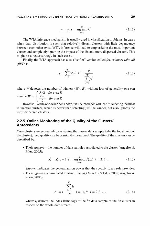
y ¼ yi; i ¼ arg minR

l¼1ll ð2:11Þ

The WTA inference mechanism is usually used in classification problems. In cases

when data distribution is such that relatively distant clusters with little dependency

between each other exist, WTA inference will lead to emphasizing the most important

cluster and completely ignoring the impact of the distant, more dispersed clusters. This

might be a better strategy in such cases.

Finally, the WTA approach has also a “softer” version called few-winners-take-all

(fWTA):

y ¼XWi¼1

liyi; li ¼ tiXWl¼1

tlð2:12Þ

where W denotes the number of winners (W<R); without loss of generality one can

assume W ¼R=2 for even RR�12

for odd R

(

In a case like the one described above, fWTA inferencewill lead to selecting themost

influential clusters, which is better than selecting just the winner, but also ignores the

most dispersed clusters.

2.2.5 Online Monitoring of the Quality of the Clusters/Antecedents

Once clusters are generated (by assigning the current data sample to be the focal point of

the cluster), then quality can be constantly monitored. The quality of the clusters can be

described by:

. Their support—the number of data samples associated to the cluster (Angelov &

Filev, 2005):

Sit ¼ Sit�1þ 1; i ¼ arg maxR

i¼1tiðxtÞ; t ¼ 2; 3; . . . ; ð2:13Þ

Support indicates the generalization power that the specific fuzzy rule provides.

. Their age—an accumulated relative time tag (Angelov & Filev, 2005; Angelov &

Zhou, 2006):

Ait ¼ t�

XSitl¼1

Il

Sit; i ¼ 1;R½ �; t ¼ 2; 3; . . . ð2:14Þ

where Il denotes the index (time tag) of the lth data sample of the ith cluster in

respect to the whole data stream.


The age indicates how up-to-date the information that is generalized by a certain

fuzzy rule is. Based on the age, one can simplify the fuzzy rule-based system

online by removing old rules. Based on the age dynamics (measured by the

derivative of the age) one can also detect shift and drift of the concept (Angelov&

Zhou, 2008). Figure 2.5 demonstrates the evolution of the age of fuzzy rules

(respectively clusters).

. Utility—the accumulated relative firing level of a particular antecedent (Angelov,

2006):

Uit ¼

Xtl¼1

ll

t�Ii* ; i ¼ 1;R½ �; t ¼ 2; 3; . . . ð2:15Þ

where Ii* denotes the index (time tag) of the data sample thatwasused as a focal point

of the ith fuzzy rule (in other words, it indicates when a fuzzy rule was generated).

The utility indicates how much a certain fuzzy rule was used after it was

generated—its variability represents the nonstationarity. Figure 2.6 demonstrates

the evolution of the utility of the fuzzy rules for the same problem.

. Zone of influence (radius), which can be adaptively updated (Angelov &

Zhou, 2006) and will be described in the next section.

. Local density, which is another measure of the generalization power:

LitðztÞ ¼1

1þXnþm

j¼1ðnijtÞ2

; Li1ðz1Þ ¼ 1; i ¼ 1;R½ �; t ¼ 2; 3; . . . ð2:16Þ

Figure 2.5. Evolution of the age of the clusters/fuzzy rules for the NOx estimation problem.


where ðnijtÞ2 ¼ 1Sit�1

XSit�1l¼1ðzi*j �zljÞ2 denotes the local scatter (Angelov& Filev, 2005).

It is obvious that the only difference between the global density given by (2.5) and

the local density (2.16) is the number of data points that are taken into account—in the

local density, only the points that support a particular cluster are taken into account,

whereas the global density is in respect to all data points read so far. Also it is obvious that

the local scatter can be updated recursively (Angelov & Zhou, 2006).

In data-driven models, the importance of the fuzzy rules can be evaluated by these

quality measure indicators, which also assist the evolution process.

2.2.6 Online Structure Simplification (Marginal Rules Removal)

The structure of the evolving fuzzy system is open—the rule base can grow by generating

new fuzzy rules but it can also shrink by removing rules that are:

. Outdated (old, that is with high age).

. With low support, that is, with low generalization power (in order for a rule to

be established, its focal point must have high generalization power at the

moment of its generation, but this may change later due to the online nature of

the process).

. With low utility, that is, the data pattern shifted away from the focal point of that

rule.

Figure 2.6. Evolution of the utility of the clusters/fuzzy rules for the NOx estimation problem.


Any of these cases may lead to disabling a fuzzy rule by assigning zero to the

normalized firing level:

Condition C1 : IF Uit < �Ut�Ut

� �THEN ðR R�1Þ ð2:17Þ

Condition C2 : IF ðAit >

�Atþ AtÞ THEN ðR R�1Þ ð2:18Þ

Condition C3 : IF ðSit < 3Þ AND ðt � Ii*þ 10Þ THEN ðR R�1Þ ð2:19Þ

where �Ut denotes themean utility after t data are read; Ut denotes the standard deviation

of the utility after t data are read; �At denotes the mean age at moment t; At denotes the

standard deviation of the age after t data are read.

As an alternative to Condition C1, Angelov and Filev 2005 proposed to use a

threshold, h (suggested values are [0.03; 0.1]), in the following way:

ConditionC01 : IF ðUit < hÞ THEN ðR R�1Þ ð2:17aÞ

Based on these principles, and satisfying the remaining aims, the algorithm, called

eClusteringþ , is proposed.

Pseudocode of eClusteringþ

Algorithm eClusteringþBegin eClustering+

Read the input-output pair, zt

IF (t = 1) THEN (Initialise)

ELSE

Calculate recursively the data density around by

(2.6);

Update recursively the density of the focal points

by (2.7);

IF (Condition A) THEN (form a new focal point, R R +1;

zi* zt; D(z

i*) 1; I

i* 1) ;

IF (Condition B) THEN (remove the rule for which

it holds)

Assign the current data sample to the nearest cluster

(to the rule it satisfies most);

END IF

Repeat the procedure until end of the data stream or

external request to stop

END eClustering+

Notes:

1. Initialize includes initialization (if possible) or assigning the input part of the firstavailable data point to become the focal point of the first cluster (“starting fromscratch”): x1* x1; R 1; Dðx1*Þ 1; b1 0; cj1 0.

2. Condition A may be realized as A1 or A2.


2.3 PARAMETER IDENTIFICATION BY fwRLS METHOD

Once the structure of the evolving fuzzy system eTSþ is defined and established, the

problem of parameter identification becomes important. It takes place only when there

are real/measured outputs (let us have tmeasured outputs out of k data samples in total;

that is, for (k� t) of the data samples we know the inputs only, t� k). One can use

supervised learning for these instances. In eTSþ , we assume that real outputs may not

always be provided. When this is the case, eTSþ produces output as an offline system

and no update and evolution takes place. When real/measured outputs are provided

(we denote them by �yt), they are used to:

. Tune (optimize) the consequent parameters of the locally linear subsystems, as

will be described below.

. Calculate the potential of the input–output pair to form a new cluster (respectively

fuzzy rule) or to replace an existing one.

. Update the cluster (respectively fuzzy rule) quality indicators and, if necessary,

remove clusters/rules that are old, with low utility and support.

Equation (2.10) can be transformed into a vector form (Angelov & Filev, 2004):

y ¼ cTq ð2:20Þ

where y ¼ ½y1; y2; . . . ym�T is the m-dimensional output of the MIMO eTSþ ;

c ¼ ½l1�xT ; l2�xT ; . . . ; ln�xT �T denotes the fuzzily weighted extended inputs vector,

�x ¼ 1; x1; x2; . . . ; xn½ �T ; q ¼ ½ðg1ÞT ; ðg2ÞT ; . . . ; ðgRÞT �T is the vector of parameters of

the rule base; and g i ¼ai01 . . . ai0m. . . . . . . . .ain1 . . . ainm

24

35T

denotes the matrix of consequent part

parameters (parameters of the ith linear local subsystem) assuming m outputs. Note

that if use fWTA (2.12), the same expressions will take place but R will have to be

substituted for byW. Note also that the time index is dropped for clarity (e.g., y ¼ cTqinstead of yk ¼ cT

kqt).

2.3.1 Local or Global Optimization

Learning and evolving eTSþ from data streams combines structure and parameter

identification, unsupervised data partitioning, and supervised consequent parameters

learning (Figure 2.7).

Each time the real/target outputs �yt are provided, the consequents’ parameters

can be updated recursively using one of the two forms of fwRLS (Angelov &

Filev, 2004)—locally or globally optimal. Both have different computational require-

ments and give somewhat different results. The error function in global terms can be

PARAMETER IDENTIFICATION BY fwRLS METHOD 33

defined as:

EG ¼Xtl¼1

��yl�cT

l ql2!min ð2:21Þ

That is, the fuzzy weights l are redistributed between the fuzzy rules and implicitly

represented through c. Thus, a compensatory (collaborative) effect of the fuzzy

aggregation takes place and the overall result is possibly a lower error overall, but a

lower transparency and higher errors locally. This problem has been discussed elsewhere

(Yen et al., 1998). The alternative is to apply a locally optimal error criterion:

EiL ¼

Xtl¼1

liðxlÞ��yl��xTl g il

2!min ð2:22Þ

Note that the local criteria are given per rule. To get the overall error criterion, we

sum them together, EL ¼XRi¼1

EiL. The fuzzy weights are outside the error per rule factor

and thus are not distributed between rules. This leads fuzzy systems designed using local

optimization criteria to have higher interpretability locally. When using the vector form,

these criteria can be rewritten as:

EG ¼�Y�YTQ

T�Y�YTQ

ð2:21aÞ

where Y is an (m t)-dimensional, Y is an R (n þ 1) t-dimensional, and Q is a

R (n þ 1)m t-dimensional matrix formed by the instantaneous values of

yl ; l ¼ ½1; t�, where yl ¼ y1l ; y2l ; . . . yml½ �T is an m-dimensional output vector,

lil ; i ¼ ½1;R�, �x, and q.

Layers 1–4

Antecedent part

Layers 5–6

Consequent part

zt=[xt,yt]eClustering+

D(zk)

xk

fwRLS

yt

yk

Figure 2.7. A schematic representation of eTSþ identification as a two-stage process (the

dashed line illustrates that the output values are fed back to eTSþ , not necessarily at each step

(t� k); when the output is not fed back, eTSþ works in prediction mode, only providing yk).


EiL ¼

�Y�XTGi

TLi�Y�XTGi

; i ¼ ½1;R� ð2:22aÞ

where X is an (n þ 1) t-dimensional, and G is an (n þ 1)m t -dimensional matrix

formed by the instantaneous values of �x and g .Solutions to the optimization problems formulated with either of the two

criteria (2.21a) or (2.22a) can be sought by using the recursive least squares (RLS)

estimation technique (Ljung, 1988). A direct application of RLS, however, may lead to

nonconvergence because the original RLS algorithm is designed under the assumption of

a fixed system structure. In eTS þ we not only have fuzzily coupled linear subsystems

and streaming data, but we also have system structure evolution, as described in the

previous section. It is true that the structural changes are much less frequent than the

sampling rate, but they still do not permit using RLS directly. This led to the introduction

of fwRLS (Angelov& Filev, 2004), which has two versions; one of them is for the global

case and the other one is for the local optimization case. We consider here only the local

version of fwRLS (L-fwRLS) and will give the reasons why. L-fwRLS gives the optimal

update of the parameters of the ith local linear subsystems:

g itþ 1 ¼ g itþCit �xt l

it �yt��xTt g it� �

; g i1 ¼ 0 ð2:23Þ

Citþ 1 ¼ Ci

t�lit C

it �xt �x

Tt C

it

1þ lit �xTt C

it�xt

; Ci1 ¼ WIðnþ 1Þðnþ 1Þ ð2:24Þ

where I ¼1 0 . . . 0

0 . . . . . . . . .. . . . . . 1 0

0 . . . 0 1

2664

3775ðnþ 1Þðnþ 1Þ

a denotes a ðnþ 1Þ ðnþ 1Þ unitary matrix, and W

denotes a large number (usually W¼ 1000).

Generally, the set of parameters that satisfy the global optimization criteria (2.21a)

differ from the set of parameters that satisfy the local criteria (2.22a). The effect that

adding a new fuzzy rule or removing one from the structurewill have on the convergence

of the L-fwRLS is significantly smaller than inG-fwRLS, because this effect is expressed

only through the fact that the values of the normalized activation levels l change. More

importantly, the covariance matrixes Ci; i ¼ ½1;R� do not change, because they are not

coupled as in the global case (Angelov & Filev, 2004). Therefore, when adding a new

fuzzy rule, a new covariance matrix is initiated, CRþ 1t ¼ IW. Globally optimal para-

meters require a more complicated update (Angelov & Filev, 2004) and the covariance

matrix is of size R(n þ 1)R(n þ 1) while the size of the covariance matrix in the

locally optimal case is just (n þ 1) (n þ 1). There are, indeed, R of these local

covariancematrixes (per rule), but thememory required is still less by a factor ofR. In the

local case the covariance matrixes are updated independently. Parameters of the new

rules that are formed online can be either initialized as shown in (2.23) or approximated

from the parameters of the existing R fuzzy rules, using them as a fuzzy rule base


(Angelov & Filev, 2004):

gRþ 1t ¼

XRi¼1

lig it�1 ð2:25Þ

Parameters of all other rules can be inherited from the previous time step when the

output was provided:

g it ¼ g it�1; i ¼ ½1;R� ð2:26ÞWhen a fuzzy rule is replaced by another rule due to Condition B, the focal point of

the new rule is close to the focal point of the rule to be replaced (this is the very reason it is

being replaced) and therefore the parameters and the covariance can be inherited by the

fuzzy rule being replaced (Angelov & Filev, 2004):

gRþ 1t ¼ g i*t�1; m

i*j ðxtÞ > e�1; 8j; j ¼ ½1; n� ð2:27aÞ

CRþ 1t ¼ Ci*

t�1; mi*j ðxtÞ > e�1; 8j; j ¼ ½1; n� ð2:27bÞ

It is interesting to note that whereas the expectation is for the globally optimal

parameters to ensure a lower error as compared with the locally optimal parameters,

which have the advantage of higher interpretability (Yen et al., 1998), the test results

indicate that this is not always the case. Several benchmark problems were tested

(courtesy ofMr.X. Zhou,who performed the tests) using both local and global optimality

criteria. Figure 2.8 presents the results of the test in which both models start learning

“from scratch,” learning during the whole data stream (t¼ k, there is no separate

validation data set, and after each sample a prediction ismade and at the next time step the

true value of the output is used for updating the eTSþ ).

0

0.1

0.2

0.3

0.4

0.5

0.6

0.7

0.8

Local

Global

Figure 2.8. RMSE using global and local optimization of the parameters (from left to right: Six

different data streams are presented—Mackey-Glass, Box-Jenkins, NOx, HVAC, AutoMPG,

Polypropylene).


The same number of fuzzy rules were generated in both cases (this is not unexpected

because the structure identification in both cases is the same). It was also noticed that the

computation time of the locally optimized version is significantly lower compared to the

alternative case.

Note that when local optimization criteria are used for parameter identification, the

removal of a rule from the rule base does not affect the R� 1 covariance matrixes of the

remaining rules in the rule base, each one of which has dimension (n þ m) (n þ m). It

does, however, affect the optimality of the parameters that were adapted using the fuzzily

weightedRLSmethod, but this damage can be considered as noisewithwhich the fwRLS

can cope. If a global optimization criteria is used (Angelov&Filev, 2004), the covariance

matrix combines the cross-effect of all rules and is much bigger (of size R(n þ m)R

(n þ m)) and a removal of a rule leads to deletion of (n þ m) columns and rows from it.

Analyzing the process we can conclude that the local optimization of parameters

provides a simpler (using significantly smaller covariance matrixes) and more stable

and robust solution (changes affect only one of the R covariance matrixes compared to a

change in the dimension of a large covariance matrix by adding or removing a number of

columns and rows), which ismore interpretable, and in a number of practical cases is also

more precise.

Additionally, the removal of marginal rules (Condition C) does affect the local

version of the algorithm to a much smaller degree (through l only) than the global

version, where the covariance matrix C is also being affected. Therefore, while having

both versions in eTSþ the local optimization of parameters will be considered as the

default.

2.3.2 Adaptation of the Cluster Radius (Zone of Influence)

The (usually Gaussian) membership function was defined by equation (2.5). The cluster

radius s is an important parameter that affects the results because it is part of the

membership function and thus of the activation level of the fuzzy set. It also defines the

spread of the linguistic variable that might be assigned to the projection of the cluster on

the axes. In eClustering (Angelov, 2004), the radius was assumed to be predefined in the

same way as in mountain (Yager & Filev, 1994) and subtractive clustering (Chiu, 1994)

approaches. In (Angelov & Zhou, 2006) a variable radius was introduced, which learns

the data distribution:

sijt ¼ asi

jtþð1�aÞnijt; sij1 ¼ 1; j ¼ ½1; nþm� ð2:28Þ

where a is a learning constant (the value of a¼ 1 is assumed without loss of generality).

It has to be noticed that the absence of problem-specific parameters is an obvious

advantage in any algorithm (this is especially true for online algorithms). Whereas the

parametera is suitable for all problems, thevalue of the radius is to a great extent problem

specific (although suggested values in range [0.3;0.5] for normalized data are also

relatively problem independent, it can be demonstrated that it does affect the results).

Figure 2.9 illustrates the evolution of the radius in eTSþ .


FromFigure 2.9 one can see that the radii of all the clusters converge to a stable value

pretty quickly.

2.3.3 Online Input Variables (Features) Selection

So far we have assumed that the number of input variables n is predefined and fixed. This

is very often the case because the factors that affect the output are usually known from the

prior knowledge. In many problems, however, there is a large number of (often)

correlated inputs, and input variable selection (also known in classification literature

as feature selection (Duda et al., 2000)) is a very important problem. This is especially

true for inferential (intelligent) sensors (Fortuna et al., 2007; Kordon et al., 2003). This

problem is usually considered in offline mode as a part of the preprocessing and is

usually approached using principal component analysis (PCA) (Li et al., 2000), GA

(Smits et al., 2006), partial least squares (PLS) (Fortuna et al., 2007), and sensitivity

analysis (Hastie et al., 2001).

It is often difficult to obtain representative data of dynamic and nonstationary

systems that will permit extracting the best subset of input variables. Therefore, it is

important to develop amethod that enables automatic input variable selection on-the-fly.

Having such a technique, the starting fuzzy rule-based system may encompass all

available inputs and can automatically trim the structure in all directions:

. Horizontally (online input variables selection, Condition D)

. Vertically (adding or removing fuzzy rules by eClusteringþ , age, utility, Con-

ditions B and C for shrinking the rule base, and ConditionA for expanding the rule

base)

Figure 2.9. Evolution of the radius.


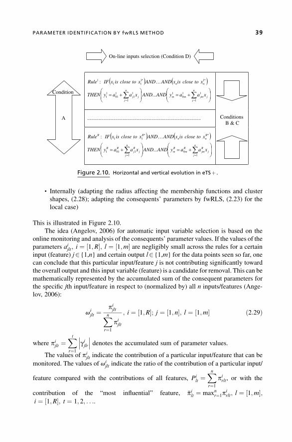
. Internally (adapting the radius affecting the membership functions and cluster

shapes, (2.28); adapting the consequents’ parameters by fwRLS, (2.23) for the

local case)

This is illustrated in Figure 2.10.

The idea (Angelov, 2006) for automatic input variable selection is based on the

online monitoring and analysis of the consequents’ parameter values. If the values of the

parameters aijlt; i ¼ ½1;R�; l ¼ ½1;m� are negligibly small across the rules for a certain

input (feature) j2 {1,n} and certain output l2 {1,m} for the data points seen so far, one

can conclude that this particular input/feature j is not contributing significantly toward

the overall output and this input variable (feature) is a candidate for removal. This can be

mathematically represented by the accumulated sum of the consequent parameters for

the specific jth input/feature in respect to (normalized by) all n inputs/features (Ange-

lov, 2006):

vijlt ¼

pijltXnr¼1

pijlt

; i ¼ 1;R½ �; j ¼ 1; n½ �; l ¼ 1;m½ � ð2:29Þ

where pijlt ¼Xtr¼1

g ijlr denotes the accumulated sum of parameter values.

The values of pijlt indicate the contribution of a particular input/feature that can be

monitored. The values of vijlt indicate the ratio of the contribution of a particular input/

feature compared with the contributions of all features, Pilt ¼

Xnr¼1

pirlt, or with the

contribution of the “most influential” feature, �pilt ¼ maxnr¼1pirlt; l ¼ ½1;m�;

i ¼ ½1;R�; t ¼ 1; 2; . . ..

On-line inputs selection (Condition D)

n

jjjmmm

n

jjj

nn

xaayANDANDxaayTHEN

xtocloseisxANDANDxtocloseisxIFRule

1

110

1

1

11

101

11

*1*111

1

...

:

..........................................................................................

n

jj

Rjm

Rm

Rm

n

jj

Rj

RR

Rnn

RR

xaayANDANDxaayTHEN

xtocloseisxANDANDxtocloseisxIFRule

10

11011

**11

...

:

Condition

A Conditions B & C

Figure 2.10. Horizontal and vertical evolution in eTSþ .


An extensive empirical study (Angelov & Zhou, 2008) indicates that, whereas the

former is more appropriate for problems with high dimensional input (e.g., more than

10), for problems with a smaller dimension of the input (number of features) (e.g., 10,

which is very often the case), the latter is more appropriate because it is more

representative.When the number of features is large, the sumof contributionsP becomes

a large number on its own and masks the effect of a particular feature. Therefore, the

comparison in this case is with the feature that contributes most, �p. Finally, the followingcondition for removal of less relevant inputs (features) and thus for horizontal adaptation

of the fuzzy system is proposed (Angelov, 2006):

Condition D1 :IF�9j*jvi

j*lt < ePilt

ANDðn � 10Þ THENðremove j*Þ

where i ¼ ½1;R�; l ¼ ½1;m�; t ¼ 2; 3; . . .ð2:30aÞ

Condition D2 :IF�9j*jvi

j*lt < e�pilt

ANDðn > 10Þ THENðremove j*Þwhere i ¼ ½1;R�; l ¼ ½1;m�; k ¼ 2; 3; . . .

ð2:30bÞ

where e denotes a coefficient (suggested values are [0.03;0.1]).

Note that a removal of a feature leads to a change in the dimension (shrinking) of a

number of variables (e.g., the vector of inputs x; the vector of focal points x�; recursivevariables b and c; and more importantly, the covariance matrix, C, parameters, a, g).

The role of the online selection of input variables is very important in the inferential

or intelligent sensors (Angelov et al., 2008). It also adds to the arsenal of tools for

autonomous evolution of fuzzy systems.

2.3.4 Online Scaling of the Input Values

The problem of treating all of the data equally is very important, especially for an online

automatic self-developing system such as eTSþ that deals with streaming data. The

values of different input variables need to be in comparable ranges in order for the

coefficients of the consequent part and in the covariance matrixes not to have extremely

high values. There are two techniques that are widely used for dealing with this

problem—normalization and standardization (Duda et al., 2000). Both of these can

be applied to the data stream online (in a recursive manner) before feeding the data to

eTSþ as detailed in Angelov and Filev (2005) for standardization and in Angelov

et al. (2007) for normalization. When comparing online normalization to the online

standardization one can conclude that the online normalization is exact because it

treats all data points equally despite the fact that the range of data may change. However,

it brings instability, because any new data point that is outside of the range so far

extends it. Standardization, on the other hand, is much more robust because the

mean and standard deviation accumulate the effects of all the data and do not change

suddenlyanddrastically.Therefore, bydefault, in eTSþ online standardization is applied,

whichconfinesover95%of the standardizeddata into the range [�2;2] (Dudaet al., 2000).


The standardization is based on the subtraction of the mean and normalizing by the

standard deviation of the data (Duda et al., 2000):

zjt ¼ zjt��zjtzjt

; j ¼ 1; n½ �; t ¼ 2; 3; . . . ð2:31Þ

where zjt denotes the standardized value of the jth input variable (feature) at the tth time

instant; �zjt ¼ 1t

Xtl¼1

zjl ; j ¼ 1; n½ �; t ¼ 2; 3; . . . denotes the mean per input variable

(feature); and zjt denotes the standard deviation of the jth input/feature calculated based

on t data samples.

Both the mean and the standard deviation can be updated recursively (Angelov &

Filev, 2005) by:

�zjt ¼ t�1t

�zjðt�1Þ þ 1

tzjðt�1Þ; �zj1 ¼ 0; j ¼ 1; nþm½ �; t ¼ 2; 3; . . . ð2:32aÞ

z2jt ¼t�1t

z2jðt�1Þ þ1

t�1�zjt��zjðt�1Þ

; zj1 ¼ 0; j ¼ 1; nþm½ �; t ¼ 2; 3; . . . ð2:32bÞ

In order to simplify the notations we assume that the input–output vector z has been

standardized and will use z having in mind z. In order to return to the original scale, the

following transformation has to take place:

zjt ¼ zjt zjtþ�zjt; j ¼ ½1; nþm�; t ¼ 2; 3; . . . ð2:33Þ

2.4 NONLINEAR REGRESSION AND TIME-SERIES PREDICTIONUSING eTSþ

The TS fuzzy system with evolving structure (as described in Section 2.2) and adaptive

parameters learned online (as described in the previous section) is a very flexible

construct that can be applied to a range of problems, such as:

. Regression models of the type yk ¼ f ðxkÞ. Note that only a subset of the outputs

are supposed to be measured, �yt; t � k.

. Time-series prediction or filtering, for example, yt ¼ f ðxt�1; . . . ; xt�Nx;yt�1; . . . ; yt�NyÞ, which is also known as nonlinear autoregressionwith exogenousinput (NARX) or as nonlinear output error (NOE), when the past predictions are

used instead of the actual data.

. Classification, when the output is the class label that is implemented in the eClass0

approach (Angelovet al., 2007), orwhen the classification surface is approximated

by eTSþ , which is implemented in eClass1 and eClassM (Angelov &

Zhou, 2008b).

NONLINEAR REGRESSION AND TIME-SERIES PREDICTION USING eTS þ 41

. Clustering or novelty detection (Angelov et al., 2008).

. Control (Angelov, 2004b).

The flowchart of the eTSþ algorithm is given in Figure 2.11.

One particular application of eTSþ for regression is its implementation as an

inferential sensor, called eSensor (Angelov et al., 2008), which is schematically

represented in Figure 2.12.

*x = eClustering+ (xt-1,yt-1)

t=1yes

1;1;1;1

;1;5.0;0

0;1;

111

111

111*1

LUS

Ac

bDxxjj

)6.2(byzD tt

)7.2(** byzD tt

Condition A no

Form new rule around xt

Condition B

Remove old rule

yes

Condition C

Remove rule

Condition D

(a)

Remove input

Return *x

yes

yes

Figure 2.11. a. Flowchart of the eClusteringþ part of eTSþ . b. Flowchart of eTSþ .


2.5 APPLICATION OF eTSþ

In this section we use a data stream generated by conventional sensors mounted on car

engines subjected to tests (courtesy of Dr. E. Lughofer, University of Linz, Austria). In

this experiment, initially 180 different physical variables were measured using conven-

tional (hard) sensors. Most of these potential inputs to the regression model are the same

physical variables (such as pressure in the cylinders, engine torque, rotation speed, etc.)

measured at different time instances (different time delays). The aim is to evaluate the

*x = eClustering+ (xt-1,yt-1)

On-line scaling by (2.32)

t=1yes

111 ;;0 yyICii

)24.2()23.2(1 byt

)10.2(),3.2()2.2(byy

Rescale by (2.33)

(b)

Return y

y= eTS+ (xt, xt-1, yt-1)

Figure 2.11. (Continued)

Car engine exhaust

Hardsensors

pressure

Torque

NOx_prediction (k)

...

...

NOx_real (t)

D

Delay

rpm

-

eTS+

error (t)

Figure 2.12. eSensor for the NOx emissions (D denotes online inputs selection using Condition

D; t�k).

APPLICATION OF eTS þ 43

content ofNOx in the emissions from the exhaust automatically, possibly in real time and

adaptively. The proposed method, eTSþ , is used to generate automatically and evolve a

nonlinear regressionmodel from the input data streams. The performancewas compared

with alternative methods (Kasabov& Song, 2002; Lughofer, 2005) and with the original

version of eTS (Angelov & Filev, 2003), which is using global optimization and fixed

radius (r¼ 0.3) for all inputs/features.

The problem of selecting a small subset of the highly correlated inputs is not easy

and is usually done subjectively, based on the prior knowledge, experience, or offline

methods. In Angelov and Lughofer (2008), five inputs were used. Using eTSþ one can

start processing all 180 inputs and automatically select the best subset online. This

horizontal evolution leads to a removal of 122 different inputs. If the online input

selection (ConditionD2) is applied togetherwith theutility-basedmarginal rules removal

(Condition C1), the structure simplifies to 4 inputs and 4 well-interpretable fuzzy rules

only! All the results are tabulated in Table 2.1 (the default values for h and e of 0.1 wereused for conditions C and D respectively). One can see that the prediction error is lower

with the model that has inputs selected automatically and the time needed for calculation

is reduced significantly. Note that FLEXFIS and one of the implementations of the

original eTS algorithm have been applied to 5 preselected (using prior knowledge and

offline preprocessing) inputs/features. Despite the features being preselected offline, the

precision is not higher than using eTSþ , which selects the features online.

The online input variables selection process is illustrated in Figure 2.13. It is

interesting to notice from Table 2.1 that removing marginal rules helps reduce the

number of inputs selected at the end. This can be explained by the fact that ConditionD is

T A B L E 2.1. Performance of Different Versions of eTS on the NOx Emissions EstimationProblem and a Comparison with Other Evolving Fuzzy Systems Approaches

Method #inputs #rules RMSE Correlation

Comput.

time1, s

DENFIS2 180 413 0.17 0.917 96

eTS (original3) 180 22 0.19 0.839 59.32

eTS (original4) 5 (preselected) 3 0.17 0.915 0.76

FLEXFIS4 5 (preselected) 5 – 0.911 3.16

Feedforward NN5 180 2 hidden layers 0.15 0.934 1.8

15 neurons each

exTS6 180 22 0.17 0.914 0.282

eTSþ (D only)7 58 40 0.14 0.943 0.134

eTSþ (C1 only)7 180 7 0.15 0.929 0.158

eTSþ (D & C1)7 4 4 0.14 0.939 0.026

1 Simulations were carried out using Matlab� on a laptop equipped with memory 1GB and Intel�U2500CPU.2 (Kasabov & Song, 2002).3 (Angelov & Filev, 2004).4 (Angelov & Lughofer, 2008).5 Using Matworks�.6 (Angelov & Zhou, 2006).7 Introduced first in Angelov (2006).


checked for each rule one by one, rather than on all rules as awhole. Dropping amarginal

rule leads to removal of some inputs, which causes the relevant inputs to also drop out.

The Mackey-Glass chaotic time series is generated from the Mackey-Glass differ-

ential delay equation defined by Asuncion and Newman (2007):

dM

dt¼ 0:2Mðt�tÞ

1þM10ðt�tÞ�0:1MðtÞ ð2:34Þ

The aim is to use the past values of x to predict some future value of x. We assume

x(0)¼ 1.2, t¼ 17 and the value of the signal 85 steps ahead x(t þ 85) is predicted based

on the values of the signal at the current moment, 6, 12, and 18 steps back:

y ¼ Mtþ 85; x ¼ ½Mt�18; Mt�12; Mt�6; Mt�T ð2:35Þ

The training data set consists of 3000 data samples and the validation data set of 500

data samples. The nondimensional error index (NDEI) is defined as the ratio of the root

mean square error over the standard deviation of the target data (Kasabov&Song, 2002).

Note that this particular benchmark data set (Mackey-Glass time series) has four inputs

only and conditionD is not particularly necessary, and thenumberof fuzzy rules generated

is not excessively large by applying the original (Angelov & Filev, 2004) and extended

(Angelov & Zhou, 2006) versions of eTS, and, therefore, the effect of the improvements

eTSþ brings is primarily in the smaller time required for computations because of the use

of local learning. Note that eTSþ can also work in global learning mode.

2.6 CONCLUSION AND OUTLOOK

In this chapter a new and enhanced version of the popular evolving Takagi-Sugeno

approach (Angelov& Filev, 2004) is introduced, called eTSþ . It builds on the strengths

of the original eTS; namely, it is also fully recursive (thus suitable for online applications

T A B L E 2.2. Test with Mackey-Glass Time Series1

Method #rules RMSE NDEI2Computational

time, s

DENFIS 27 0.102 0.404 1.4

eTS (original, r¼ 0.25) 9 0.094 0.373 0.473

Feedforward NN 2 15 neurons 0.122 0.441 7.6

Kalman filter3 1 0.117 0.462 0.24

exTS 12 0.080 0.320 0.83

eTSþ (C1 only) 8 0.111 0.438 0.08

eTSþ (D & C1) 10 0.099 0.392 0.09

1More details about this benchmark problem can be found in Asuncion and Newman (2007); conditions of the

test are the same as for the previous experiment.2 Nondimensional error index—described in more detail for example, in Angelov and Filev (2004).3 Kalman (1960).

CONCLUSION AND OUTLOOK 45

and computationally light), robust, flexible, and autonomous (can start from scratch and

does not use thresholds or user-specific parameters). It has, however, additional

advantages—namely, alternative mechanisms that allow shrinking of the rule base as

well as its growth based on age and utility of the rules; online input variables selection

(horizontal evolution); and alternative conditions for forming rules. It does not neces-

sarily assume that each data samplewill have real/target output. It also has a variable zone

of influence of the clusters that are used to form fuzzy rules, and can have multiple

outputs (MIMO structure). It has been demonstrated on the test example using real data

0 20 40 60 80 1000

0.5

1

1.5

2

2.5

3

3.5

Inputs weights/importance based on learning using100 data samples

Acc

umul

ated

val

ue o

f out

put p

aram

eter

s, w

0 1 2 3 4 5 6 70

5

10

15

20

25Inputs weights/importance based on learning on

200 data samples

inputs selected after learning on 200 data samples

Acc

umul

ated

val

ue o

f the

out

put p

aram

eter

s, w

Figure 2.13. Online input variables selection (Condition D) for the NOx test problem; top

plot—a snapshot after 100data samples have been read; secondplot—a snapshot after 200 data

samples have been read; third plot—a snapshot after 300 data samples have been read; bottom

plot—the finally selected features.


that the proposed improvements, which are subject to a pending patent (Angelov, 2006),

lead to significantly improved results of eTSþ . Awide range of industrial and research

applications of eTSþ are currently under investigation.

2.7 ACKNOWLEDGMENTS

The author would like to extend thanks to Mr. Xiaowei Zhou, for assistance in tests and

experiments, to Dr. Edwin Lughofer, for providing the data for the NOx problem, and to

Prof. Fernando Gomide, for useful feedback on the manuscript.

0 1 2 3 4 5 60

10

20

30

40

50

60

70Inputs weights/importance based on learning on

300 data samples

Inputs selected based on learning using 300 data samples

Acc

umul

ated

val

ue o

f out

put p

aram

eter

s, w

0.5 1 1.5 2 2.5 3 3.5 4 4.50

20

40

60

80

100

120

Inputs weights/importance at the end of learning based on all data samples

Inputs selected finally

Acc

umul

ated

val

ue o

f out

put p

aram

eter

s, w

Figure 2.13. (Continued)

ACKNOWLEDGMENTS 47

2.8 REFERENCES

Angelov, P., R. Buswell (2001). “EvolvingRule-BasedModels: ATool for Intelligent Adaptation.”

Proc. 9th IFSA World Congress, Vancouver, BC, Canada, July 25–28, 2001, pp. 1062–1067.


Heidelberg, New York; Springer-Verlag, ISBN 3-7908-1457-1.

Angelov, P., R. Buswell (2003). “AutomaticGeneration of FuzzyRule-BasedModels fromData by

Genetic Algorithms,” Information Sciences, Vol. 150, No. 1/2, pp. 17–31.

Angelov, P., D. Filev (2003). “On-line Design of Takagi-Sugeno Models,” In: Lecture Notes in

Computer Sci., Vol. 2715, Fuzzy Sets and Systems, IFSA2003 ( T. Bilgic, B. De Baets, O.

Kaynak, eds.), pp. 576–584.

Angelov, P. (2004). “An Approach for Fuzzy Rule-Based Adaptation Using On-line Clustering,”

Int. Journal of Approximate Reasoning, Vol. 35, No. 3, pp. 275–289.

Angelov, P. P. (2004b). “A Fuzzy Controller with Evolving Structure,” Information Sciences, Vol.

161, pp. 21–35, ISSN 0020-0255.


Models.” IEEE Trans. on System, Man, and Cybernetics, Part B—Cybernetics, Vol. 34, No. 1,

pp. 484–498, ISSN 1094-6977.

Angelov, P., C. Xydeas, D. Filev (2004a). “On-line Identification of MIMO Evolving Takagi-

Sugeno Fuzzy Models.” Proc. International Joint Conference on Neural Networks and

International Conference on Fuzzy Systems, IJCNN-FUZZ-IEEE, Budapest, Hungary, July

25–29, 2004, pp. 55–60, ISBN 0-7803-8354-0.

Angelov, P., J. Victor, A. Dourado, D. Filev (2004b). On-line Evolution of Takagi-Sugeno Fuzzy

Models. Proc. 2nd IFAC Workshop on Advanced Fuzzy/Neural Control, Oulu, Finland,

September 16–17, 2004, pp. 67–72.

Angelov, P., D. Filev (2005). “Simpl_eTS: A Simplified Method for Learning Evolving Takagi-

Sugeno Fuzzy Models.” 2005 IEEE Int. Conference on Fuzzy Systems, FUZZ-IEEE, Reno,

Nevada, May 22–25, 2005, pp. 1068–1073, ISSN 0-7803-9158-6/05.

Angelov, P. (2006). Machine Learning (Collaborative Systems) Patent ( WO2008053161, priority

date—November 1, 2006; international filing date October 23, 2007).


2006 Int. Symposium on Evolving Fuzzy Syst., Ambleside, UK, September 7–9, 2006, IEEE

Press, pp. 29–35, ISBN 0-7803-9719-3.

Angelov, P., X. Zhou, F. Klawonn (2007). “Evolving Fuzzy Rule-Based Classifiers.” 2007 IEEE

Int. Conference on Computational Intelligence Applications for Signal and Image Processing,

Honolulu, Hawaii, April 1–5, 2007, IEEE Press, pp. 220–225.

Angelov, P., E. Lughofer (2008). “A Comparative Study of Two Approaches for Data-Driven

Design of Evolving Fuzzy Systems: eTS and FLEXFIS.” Int. Journal onGeneral Systems, Vol.

37, Issue 1, February 2008, pp. 45–67.

Angelov, P., X. Zhou (2008a). “On Line Learning Fuzzy Rule-based System Structure from Data



Angelov, P., X. Zhou (2008b). “Evolving Fuzzy Rule-Based Classifiers fromData Streams.” IEEE

Transactions on Fuzzy Systems, Vol. 16 (6), Special Issue on Evolving Fuzzy Systems,

pp. 1462–1475.


Angelov, P., R. Ramezani, X. Zhou (2008a). “AutonomousNovelty Detection andObject Tracking

in Video Streams Using Evolving Clustering and Takagi-Sugeno Type Neuro-Fuzzy System.”

World Congress on Computational Intelligence, Hong Kong, June 1–6, 2008, pp. 1457–1464,

ISBN 978-1-4244-1821-3/08.

Angelov, P., A. Kordon, X. Zhou (2008b). “Evolving Fuzzy Inferential Sensors for Process

Industry.” Proc. 3rd International Workshop on Genetic and Evolving Fuzzy Systems, Wit-

ten-Bomerholz, Germany, March 4–7, 2008, IEEE Press, pp. 41–46, ISBN 978-1-4244-1613-4.

Angelov, P., C. D. Bocaniala, C. Xydeas, C. Pattchet, D. Ansell, M. Everett, G. Leng (2008c). “A

Passive Approach to Autonomous Collision Detection and Avoidance in Uninhabited Aerial

Systems” Proc. 2008 EUROSIM, Emanuel College, Cambridge, UK, April 1–3, 2008, pp.

64–69.


Asuncion, A., D. Newman (2007). “UCI Machine Learning Repository’’, http://mlearn.ics.uci.

edu/MLRepository.html.

Chiu, S. (1994). “Fuzzy Model Identification Based on Cluster Estimation,” Journal of Intelligent

and Fuzzy Systems, Vol. 2 (3), pp. 267–278.

Domingos, P., G. Hulten (2001). “Catching Up with the Data: Research Issues in Mining Data

Streams.” Workshop on Research Issues in Data Mining and Knowledge Discovery, Santa

Barbara, CA, 2001.

Duda, R. O., P. E. Hart, D. G. Stork (2000). Pattern Classification—Second Edition. Chichester,

West Sussex, England: Wiley-Interscience.

EC (2007). “NMP-2008-3.2-2—Self-Learning Production Systems.” Work Programme on

Nanosciences, Nanotechnologies, Materials and New Production Technologies, available

online at ftp://ard.huji.ac.il/pub/251/NMP_Fiche_small__2008_02.pdf.

Elgammal, A., R. Suraiswami, D. Harwood, and L. Davis (2002). “Background and Foreground

Modeling Using Non-parametric Kernel Density Estimation for Visual Surveillance KDE,”

Proc. 2002 IEEE, Vol. 90, No. 7, pp. 1151–1163.

Fortuna,L., S.Graziani,A.Rizzo,M.G.Xibilia (2007). “Soft Sensor forMonitoring andControl of

Industrial Processes. In Advances in Industrial Control Series ( M. J. Grimble, M.A. Johnson,

eds.). Berlin, Springer-Verlag.

Hastie, T., R. Tibshirani, and J. Friedman (2001). The Elements of Statistical Learning: Data

Mining, Inference and Prediction. Heidelberg: Springer-Verlag.

Jang, J. S.R. (1993). “ANFIS: Adaptive Network-Based Fuzzy Inference Systems.” IEEE Trans.

on SMC, Vol. 23, No. 3, pp. 665–685.

Kalman, R. (1960). “A New Approach to Linear Filtering and Prediction Problems.” Trans. of the

ASME—Journal of Basic Engineering, Vol. 82, pp. 35–45.

Kasabov, N., Q. Song (2002). “DENFIS: Dynamic Evolving Neural-Fuzzy Inference System and

Its Application for Time-Series Prediction.” IEEE Trans. on Fuzzy Systems, Vol. 10, No. 2, pp.

144–154.

Kordon, A., G. Smits, A. Kalos, and E. Jordaan (2003). “Robust Soft Sensor Development Using

Genetic Programming.” In Nature-Inspired Methods in Chemometrics (R. Leardi, ed.).

Amsterdam: Elsevier, pp. 69–108.

Li, W., H. H. Yue, S. Valle-Cervantes, and S. J. Qin (2000). “Recursive PCA for Adaptive Process

Monitoring.” Journal of Process Control, Vol. 10 (5), pp. 471–486.

Ljung, L. (1988). System Identification, Theory for the User. Englewood Cliffs, NJ: Prentice-Hall.

REFERENCES 49

Lughofer, E., E. Klement (2005). “FLEXFIS: A Variant for Incremental Learning of Takagi-

Sugeno Fuzzy Systems,” Proc. FUZZ-IEEE 2005, Reno, Nevada, pp. 915–920.

Patchett, C., V. Sastri (2007). “Decision Architectures for Uninhabited Autonomous Aerial

Systems.” EuroSim 2007, Ljubljana, Slovenia, September 9-13, 2007.

Qin, S. J., H.Yue, andR.Dunia (1997). “Self-Validating Inferential SensorswithApplication toAir

Emission Monitoring,” Industrial Engineering Chemistry Research, Vol. 36, pp. 1675–1685.

Roubos, J., M. Setnes, J. Abonyi (2003). “Learning Fuzzy Classification Rules from Data.”

Information Sciences, Vol. 150, pp. 77–93.

Silva, L., F. Gomide, R. R. Yager (2005). “Participatory Learning in Fuzzy Clustering.” Proc. 24th

IEEE International Conference on Fuzzy Systems, FUZZ-IEEE, Reno, Nevada, May 22–25,

2005, pp. 857–861, ISSN 0-7803-9158-6/05.

Smits, G., A. Kordon, E. Jordaan, C. Vladislavleva, M. Kotanchek (2006). “Variable Selection in

IndustrialData SetsUsing ParetoGenetic Programming,” InGenetic Programming Theory and

Practice III. (T. Yu, R. Riolo, B. Worzel, eds.). New York: Springer, pp. 79–92.

Sugeno, M., K. T. Kang (1988). “Structure Identification of Fuzzy Model.” Fuzzy Sets and

Systems, Vol. 28, No. 1, pp. 15–23.

Takagi, T., M. Sugeno (1985). “Fuzzy Identification of Systems and Its Applications to Modeling

and Control.” IEEE Trans. on Systems, Man and Cybernetics, Vol. 15, No. 1, pp. 116–132.

Wang, L., J. Mendel (1992). “Fuzzy Basis Functions, Universal Approximation and Orthogonal

Least-Squares Learning.” IEEE Trans. on Neural Networks, Vol. 3, No. 5, pp. 807–814.

Yager, R., D. Filev (1994). “Approximate Clustering via the Mountain Method.” IEEE Trans. on

Systems and Cybernetics, Vol. 24, No. 8, pp. 1279–1284.

Yen, J., L.Wang, C.W. Gillespie (1998). “Improving the Interpretability of TSK FuzzyModels by

Combining Global and Local Learning,” IEEE Trans. Fuzzy Syst., Vol. 6, pp. 530–537.

Zadeh L. A. (1975). “The Concept of a Linguistic Variable and Its Application to Approximate

Reasoning: Parts I, II, and III,” Information Sciences, Vol. 8, pp. 199–249, 301–357; vol. 9,

pp. 43–80.


3

FUZZY MODELS OF EVOLVABLEGRANULARITY

Witold Pedrycz

In real-world scenarios, we are often faced with nonstationary phenomena whose

parameters or even structures change over time and/or space. The underlying systems

evolve. Subsequent models of such phenomena, including fuzzy models, describing

these phenomena have to evolve so that they stay relevant. Considering the inherent

granularity present in fuzzy modeling, the objective of this study is to endow fuzzy

models with an important feature of evolvable granularity—granularity whose level

mirrors the varying dynamics and perception of the data/system. Depending on the

architecture of the fuzzymodels, the changes in granularity can be directly translated into

the number of rules, local models, number of fuzzy neurons, and so on. As information

granularity is positioned in the center of the design of such fuzzy models, we develop a

concept of dynamic data granulation realized in the presence of incoming data organized

in the form of data snapshots. For each of these snapshots we reveal a structure by

running fuzzy clustering. The proposed algorithm of adjustable Fuzzy C-Means exhibits

a number of useful features associatedwith the dynamic nature of the underlying data: (1)

The number of clusters is adjusted from one data snapshot to another in order to capture

the varying structure of patterns and its complexity, and (2) continuity between the

consecutively discovered structures is retained—the clusters formed for a certain data

snapshot are constructed as a result of evolving the clusters discovered in the prede-

ceasing snapshot. The criterion used to control the level of information granularity


and Nikola Kasabov


throughout the process is guided by a reconstruction criterion that quantifies an error

resulting from pattern granulation and de-granulation. The proposed design strategy

being focused on the evolution of information granules implies further detailed devel-

opments of local models (e.g., those forming conclusions of the associated rule-based

architecture).

3.1 INTRODUCTORY NOTES

In a number of scenarios of data analysis, we encounter collections of data being

generated over time or over space. Banking data, supermarket data, weather recordings,

sensor data, customer reports, customer segmentation, data streams and the alike—all of

them are examples of data generated over either time or space. Models describing such

phenomena need to be endowed with significant evolvable capabilities. In fuzzy

modeling we have witnessed an emergence of a new category of fuzzy models that

address the dynamics of the changes, referred to as evolvable fuzzy models [1, 2]. An

outstanding feature of models that supports their evolvability comes with a model’s

modularity. In this study, to offer a sound focus we concentrate on rule-based archi-

tectures of the form

If Ai; then fiðx; aiÞ ð3:1Þ

whereAi are information granules (fuzzy sets defined in themultivariable input space) and

fi stand for the conclusion part. In essence, the form of the conclusion could be very

diversified. We could encounter fuzzy sets, linear functions, polynomials, and neural

networks. The vector of parameters of the conclusion part is denoted by ai. In particular,

those could be the parameters of the polynomials or the connections of the neural network.

The construction of fuzzy rule-based models has been a topic of intensive design

studies and we have witnessed a great deal of important developments [12, 13, 18, 19,

21]. Particularly discussed were various issues dealing with multiobjective develop-

ments of fuzzymodels involving a satisfaction of criteria of accuracy and interpretability.

The design of rule-based topologies is naturally split into two phases:

1. Formation of the condition parts of the rules

2. Development of the conclusions of the rules

The number of rules is directly associatedwith the granularity of the fuzzymodel—a

unique feature of the class of rule-based architectures. The higher the number of the rules,

the higher the granularity of the model and the more details are captured. Quite

commonly, the condition parts of the rules are constructed with the use of fuzzy

clustering, which produces a collection of information granules—clusters formed in

the input space. Various clustering techniques have been exploited as a generic design

framework for the design of fuzzy sets and partition the input space. The development of

the conclusion part is quite standard, as in many cases it boils down to the linear

estimation problem with some eventual enhancements.

52 FUZZY MODELS OF EVOLVABLE GRANULARITY

The fuzzymodel evolves continuously by being facedwith incoming data to capture

the essence of the system that undergoes changes. Such changes could be either

continuous or abrupt. In the case of continuous changes, the model may adapt to such

modifications through the corresponding changes made to the parameters of the model.

In situations where we encounter more radical changes, the structure of the model needs

to be modified in a structural manner. In the context of fuzzy rule-based systems, the

parametric changes can be quite directly translated into continuous updates of the

parameters of the local models standing in the conclusions of the rules. In the case of

linear models, we can see here a recurrent format of the updates of the parameters that is

well documented in the literature. The structural changes are more sophisticated and

their realization is associated with the varying number of the rules. In the presence of

dynamically collected data, information granules move around, and become more

refined or generalized—all of these effects are driven by the nature of the data being

collected and their continuous changes.

In this study we will concentrate on this facet of evolvability of the fuzzy models.

We develop a general strategy, using which the number of rules (viz. the number of

fuzzy clusters) becomes modified dynamically (either reduced or extended) depending

on the current dynamics of the data (phenomenon). Once the dynamic clustering offers

this interesting opportunity of modifying the granularity of the model, in the developed

strategy we also strive for the maintenance of continuity of the information granules,

meaning that when revising the granularity of the model, we refine or generalize the

clusters starting from the configuration of information granules encountered in the

past. This algorithmic aspect is of particular relevance when dealing with iterative

schemes of fuzzy clustering (e.g., Fuzzy C-Means, FCM) where the results are affected

by the initial conditions (say randomly initialized partition matrix) the method starts

with.

The chunks (sets) of data that we use to form information granules and describe their

dynamics are referred to as data snapshots. In particular, the problem of segmentation of

temporal data [3–5, 9] falls under the same rubric as one of the possible scenarios of

dynamic clustering.

Fuzzy clustering [6, 12, 15, 18] can be regarded as a viable alternative to consider

when dealing with dynamic data granulation; however, its generic version does require

some essential changes to address the dynamics of the available data. Our ultimate

objective is to revisit and redevelop Fuzzy C-Means (FCM) so that the generic algorithm

could be efficiently used in the framework of dynamic data analysis. In particular, wewill

be interested in dynamically adjusting the number of clusters for each temporal segment

of the data (the number could be decreased so some clusters could bemerged; the number

of clusters could be also increased, leading to the split of some clusters). Further, we

consider aweighted distance function being optimized as a part of the FCMoptimization

(which leads to the selection of the relevant attributes-features).

Inwhat follows, to illustrate the essence of the problem,we consider that the datasets

are available at some data snapshots (say, temporal, spatial, or spatio-temporal segments

W1, W2, . . ., WP) as illustrated in Figure 3.1. The clusters are formed for W1 and then,

when the next snapshot becomes available (W2), the clustering is run again starting from

some initial configuration that has been inherited from W1.

INTRODUCTORY NOTES 53

As illustrated in Figure 3.1, the clustering activities are focused on data positioned

within the individual data snapshots. What is interesting is the way the clusters are built

dynamically and carried over from one data snapshot to another. The computational

facets of the problem associated directly with the FCM are outlined in more detail in

Figure 3.2. Here, two aspects of dynamic behavior of the clusters are of interest. While

the prototypes can migrate between data snapshots (which is a desirable effect as it

contributes to the continuity of the overall process of data analysis), it is interesting to

observe the changes in the number of the clusters themselves. The number of clusters is

not fixed in advance but could fluctuate from one data snapshot to another depending on

the structure of data themselves and the complexity of the underlying dynamics of the

data (that is, the underlying phenomenon generating the data).

Referring to Figure 3.2, let us elaborate in more detail on the process of clustering.

We start with the first data snapshot, run the FCMon the data present there by producing a

collection of the prototypes v1[1], v2[1], . . . , vc[1] (the number in the square bracket

denotes that those prototypes are built on the basis of the data coming from the first

segment X[1]). The number of clusters is determined by the acceptable level of the

predetermined optimization criterion.We elaborate on the computational details later on.

When running the FCM on the second data snapshot X[2], we proceed with the

1

X[1]

2

X[2]

P

X[P]

Figure 3.1. Data snapshots (W) of multivariable data X[1], X[2],. . ., X[P] and the ensuing

clustering activities along with the adjustment of the number of clusters through their splitting

or merging.

FCM FCM FCM

Figure 3.2. The concept of dynamic clustering—progression of the FCMconstructs (prototypes

and partitionmatrixes) in successive data snapshots and dynamic adjustments of the number of

the clusters (prototypes) through cluster merging and cluster split.


prototypes that were formed forX[1] and use them as the starting point when running the

FCM forX[2]. Inevitably, when iterating FCM, the prototypes change their location as a

result of revealing the topology of the actually processed data.Once done, it couldwell be

that a certain clustering quality indicator (performance index) produced there could

exceed some required threshold or could assume values that are far lower than this

threshold. In both cases, the number of clusters needs to be dynamically adjusted. In the

first case, it must be increased—we could do that by splitting the most heterogeneous

(diversified) cluster. In the second case, the number of clusters could be too high

(capturing toomany unnecessary details) and somemerging process could be of interest.

There have been some developments along the line of dynamic fuzzy clustering. The

reader may refer to [7] as this paper offers a certain way of adjusting the granularity of

findings through successive modifications of the number of clusters. Some other studies

have been reported in [8, 9] predominantly in the setting of data segmentation and

dynamic clustering, in which data streams dealt with involved patterns whose processing

must be realized in order of their appearance.

The problem of adjustable fuzzy clustering shares some similarities with a suite of

algorithms known as data streammining and time series clustering [3, 14, 20]; however,

there are also some evident differences. In terms of similarities, we are concerned with

data that are accumulated successively and whose processing (i.e., structure determi-

nation) is carried out in an incremental fashion. There are severalmeaningful differences.

First, in time series we are concerned with the factor of time, in this study the data could

be arranged timewise (as a time sequence), but this is one of the possibilities exercised in

the proposed approach. Second, the datawithin a scope of a data snapshot are not affected

by the time variable but are treated en bloc.

The organization of the study is the following. Given the formulation of the problem

already covered in this section, we concentrate on the fundamental design aspects,

namely (1) splitting and merging criteria, (2) assessment of quality of clusters that could

be directly usedwhen controlling the dynamics of the clusters and deciding on the change

of the number of clusters themselves, and (3) optimization capabilities of fuzzy

clustering (FCM), which could be exploited upfront when running the algorithm.

3.2 FUZZY C-MEANS AS AN OPTIMIZATION ENVIRONMENTFOR THE DESIGN OF INFORMATION GRANULES

Fuzzy C-Means (FCM) [6, 16, 17] is one of the commonly encountered algorithms being

used in the formation of information granules—fuzzy sets [22]. The conceptual aspects

are well reported in the literature. The method comes with a wealth of refinements and

algorithmic investigations. There are numerous case studies. We definitely do not intend

to reiterate all of those; however, we believe that there are two points worth stressing. The

first one concerns the parametric flexibility of the algorithm (which helps induce

geometry of the clusters formed in this manner). The second one elaborates on the

issue of quality of clusters and brings forward a concept of the reconstructability

criterion, using which we assess a way of moving from numeric data to information

granules (referring to it as granulation) and back to numeric quantities (de-granulation).

FUZZY C-MEANS AS AN OPTIMIZATION ENVIRONMENT FOR THE DESIGN 55

In this section, to avoid notational clutter, we abstract from the concept of data snapshots;

we will consider a data set X¼ {x1, x2, . . . xN} where xk is defined in the n-dimensional

space of real numbers and c stands for the number of clusters. As a distance function k:k,we consider a weighted Euclidean distance of the form

Xnj¼1

ðai�bjÞ2s2j

, where sj is a

standard deviation of the jth variable (feature) and a and b are n-dimensional vectors of

real numbers.

3.2.1 Fuzzification Coefficient as an Optimization Mechanismof the FCM

The objective functionminimized in the FCM algorithm is a sum of distances of patterns

x1, x2, . . ., xN from the prototypes v1, v2, . . ., vc:

Q ¼Xci¼1

XNk¼1

umikkxk�vik2 ð3:2Þ

where c is the number of the clusters. The optimization is realized with respect to the

structure, that is, the prototypes and the partition matrix U¼ [uik]. The fuzzification

coefficient (m) that assumes values greater than 1 implies directly the resulting geometry

of the fuzzy clusters. Values close to 1 (say 1.05) imply a Boolean nature of the clusters,

so most of the entries of the partition matrix are practically equal to 0 or 1.

Typically, as commonly shows up in the literature, the fuzzification coefficient (m)

assumes a value of 2.0. In this case, the membership functions resemble a Gaussian

membership function. For higher values ofm, say 3 or higher, the membership functions

start to become quite “spikey,” with the membership grade equal to 1 for the prototype,

and then rapidly decrease to zero. The average membership for each cluster is equal to

1/c. By selecting thevalue ofmwe can control the shape of themembership functions and

select the most suitable one in light of some predefined criterion.

3.2.2 Reconstruction Criterion in the Assessment of Qualityof Clusters

The number of clusters is another important design feature of the clustering algorithm.

There have been a number of cluster validity indexes [10, 11], which are geared to assess

the most “suitable” number of clusters that are supposed to correspond with the “true”

structure in the data. The inherent problem with them is that quite often one gets several

conflicting suggestions depending on which cluster validity index has been selected.

In this study, we follow a different path, which could be referred to as a granulation–

de-granulation strategy [17, 18]. In essence, once the information granules have been

formed by the FCM, we use the prototypes to represent each pattern in the form of

information granules by computing the corresponding membership degrees. At the next

step, we complete a de-granulation, which is to estimate the pattern on the basis of the

prototypes and the membership degrees. Ideally, we would expect that the result of such


de-granulation should return the original pattern. While this is quite unlikely, we may

consider the distance between the original pattern and its de-granulated version to

constitute a viable measure of quality of obtained reconstruction. Let us move to the

technical details, which provide some required formal description of the strategy. Denote

by Xi the data whose membership in the ith cluster is the highest, that is,

Xi ¼ fxk 2 Rji ¼ argk max ukðxÞg ð3:3Þ

The reconstruction error for the ith cluster is computed as the following sum of distances

between xk and its de-granulated version xk:

Vi ¼Xxk2Xi

kxk�xkk2 ð3:4Þ

where

xk ¼

Xci¼1

umikvi

Xci¼1

umik

ð3:5Þ

The maximal value of Vi, Vmax¼maxiVi, can serve as a suitable measure describing the

reconstructibility aspects provided by the information granules. By varying the number

of the clusters (c)we can affect the values ofVi and in thisway focus on selecting themost

suitable structure in the data set.

3.3 DYNAMIC FORMATION OF FUZZY CLUSTERS—SPLITTINGAND MERGING MECHANISMS

In what follows, we discuss the mechanisms of splitting and merging clusters. Before

moving into details, we note that the objective function minimized by the FCM for the

first data snapshot exploits the standard sum of distances

Q½1� ¼Xc½1�i¼1

Xxk2X½1�

umikkxk�vi½1�k2 ð3:6Þ

(here Q[1] concerns the first data snapshot). Let us also note that the number of clusters,

say c[1], may be selected on the basis of the assumed threshold level Vmax. For the first

data snapshot, we choose such c[1] for which the reconstruction error does exceed some

predefined threshold level, that is,Vmax< e; with the value of e, e> 0 is given in advance.

Here we may adjust the number of the clusters so that the required inequality is satisfied.

The choice of the threshold level can be realized by observing how much the recon-

structability criterion is affected by the number of clusters; itmightwell be thatV exhibits

DYNAMIC FORMATION OF FUZZY CLUSTERS 57

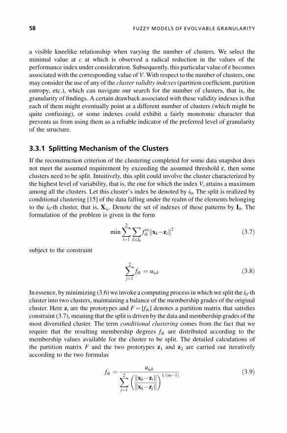
a visible kneelike relationship when varying the number of clusters. We select the

minimal value at c at which is observed a radical reduction in the values of the

performance index under consideration. Subsequently, this particular value of e becomes

associated with the corresponding value ofV. With respect to the number of clusters, one

may consider the use of any of the cluster validity indexes (partition coefficient, partition

entropy, etc.), which can navigate our search for the number of clusters, that is, the

granularity of findings. A certain drawback associated with these validity indexes is that

each of them might eventually point at a different number of clusters (which might be

quite confusing), or some indexes could exhibit a fairly monotonic character that

prevents us from using them as a reliable indicator of the preferred level of granularity

of the structure.

3.3.1 Splitting Mechanism of the Clusters

If the reconstruction criterion of the clustering completed for some data snapshot does

not meet the assumed requirement by exceeding the assumed threshold e, then some

clusters need to be split. Intuitively, this split could involve the cluster characterized by

the highest level of variability, that is, the one for which the index Vi attains a maximum

among all the clusters. Let this cluster’s index be denoted by i0. The split is realized by

conditional clustering [15] of the data falling under the realm of the elements belonging

to the i0-th cluster, that is, Xi0 . Denote the set of indexes of these patterns by I0. The

formulation of the problem is given in the form

minX2i¼1

Xk2I0

f mik kxk�zik2 ð3:7Þ

subject to the constraint

X2j¼1

fjk ¼ ui0k ð3:8Þ

In essence, byminimizing (3.6)we invoke a computing process inwhichwe split the i0-th

cluster into two clusters, maintaining a balance of the membership grades of the original

cluster. Here zi are the prototypes and F¼ [fik] denotes a partition matrix that satisfies

constraint (3.7), meaning that the split is driven by the data andmembership grades of the

most diversified cluster. The term conditional clustering comes from the fact that we

require that the resulting membership degrees fik are distributed according to the

membership values available for the cluster to be split. The detailed calculations of

the partition matrix F and the two prototypes z1 and z2 are carried out iteratively

according to the two formulas

fik ¼ ui0kX2j¼1

kxk�zikkxk�zjk� �1=ðm�1Þ ð3:9Þ


and

zi ¼

Xk2I0

f mik xkXk2I0

f mik

i ¼ 1; 2; xk 2 Xi0 ð3:10ÞThe detailed derivations of these expressions are presented in [15].

The general tendency is that with more clusters, the values of the reconstruction

criterion are getting lower. If required, further splits of the clusters could be completed

until the point the reconstruction criterion has been satisfied.

3.3.2 Merging Mechanism of the Clusters

If the objective function for the number of the clusters is lower than the predefined level e,then the number of the clusters could be reduced, meaning that some original clusters

could be combined together (merged). The way of doing that would be to merge two

prototypes that are the closest to each other. Consider that these two are indexed by s and

l, that is vs and vl. The new prototype v results from the minimization of the following

expression with respect to it; the new prototype v results from the minimization of the

following performance index:

Q ¼XNk¼1ðusk þ ulkÞmkxk�vk2!MinQwith respect to v ð3:11Þ

If for this reduced number of clusters the resulting reconstruction criterion is still lower

than the critical value, we can move on with another reduction of the number of the

prototypes. The process could be repeated by reducing the number of the clusters by one.

Let us rewrite the performance index (3.11) in a coordinate-wise fashion:

Q ¼XNk¼1ðusk þ ulkÞmkxk�vk2 ¼

XNk¼1

Xnj¼1ðuskþ ulkÞmðxkj�vj Þ2=s2j ð3:12Þ

We make the derivative of Q equal to zero,rvQ ¼ 0, and this leads to the new prototype

v ¼

XNk¼1ðusk þ ulkÞmxk

XNk¼1ðusk þ ulkÞm

ð3:13Þ

3.3.3 Processing Interaction between Results of Processingof Data Slices

Given the underlying mechanisms of merging and splitting information granules, an

overall flow of computing is displayed in Figure 3.3.

DYNAMIC FORMATION OF FUZZY CLUSTERS 59

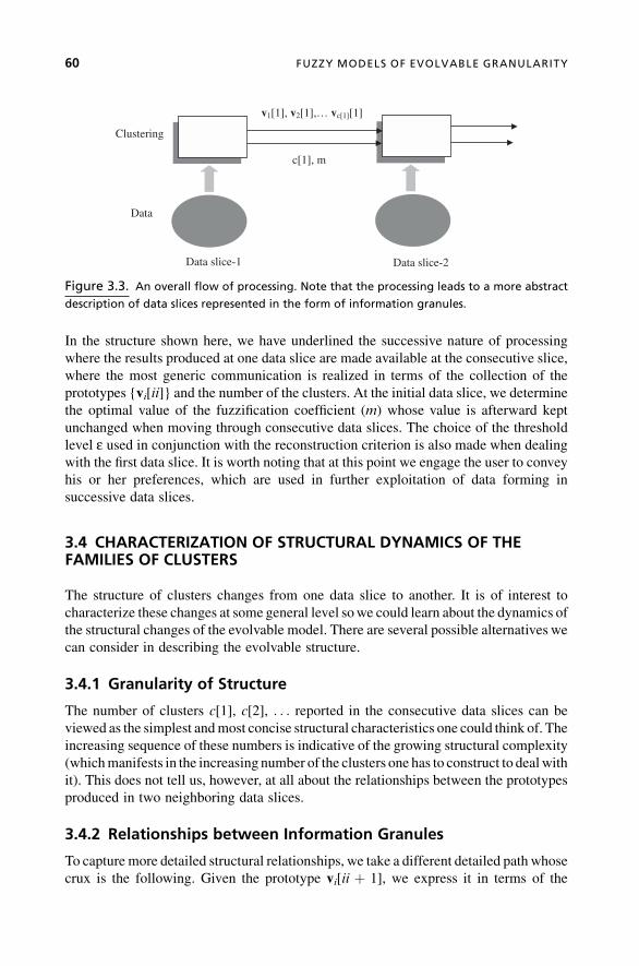
In the structure shown here, we have underlined the successive nature of processing

where the results produced at one data slice are made available at the consecutive slice,

where the most generic communication is realized in terms of the collection of the

prototypes {vi[ii]} and the number of the clusters. At the initial data slice, we determine

the optimal value of the fuzzification coefficient (m) whose value is afterward kept

unchanged when moving through consecutive data slices. The choice of the threshold

level e used in conjunction with the reconstruction criterion is also made when dealing

with the first data slice. It is worth noting that at this point we engage the user to convey

his or her preferences, which are used in further exploitation of data forming in

successive data slices.

3.4 CHARACTERIZATION OF STRUCTURAL DYNAMICS OF THEFAMILIES OF CLUSTERS

The structure of clusters changes from one data slice to another. It is of interest to

characterize these changes at some general level sowe could learn about the dynamics of

the structural changes of the evolvable model. There are several possible alternatives we

can consider in describing the evolvable structure.

3.4.1 Granularity of Structure

The number of clusters c[1], c[2], . . . reported in the consecutive data slices can be

viewed as the simplest andmost concise structural characteristics one could think of. The

increasing sequence of these numbers is indicative of the growing structural complexity

(whichmanifests in the increasing number of the clusters one has to construct to dealwith

it). This does not tell us, however, at all about the relationships between the prototypes

produced in two neighboring data slices.

3.4.2 Relationships between Information Granules

To capture more detailed structural relationships, we take a different detailed path whose

crux is the following. Given the prototype vi[ii þ 1], we express it in terms of the

Data slice-1

Clustering

c[1], m

Data slice-2

v1[1], v2[1],… vc[1][1]

Data

Figure 3.3. An overall flow of processing. Note that the processing leads to a more abstract

description of data slices represented in the form of information granules.


prototypes vj[ii] available at the iith data snapshot. More specifically, we obtain degrees

of membership of the ith prototype expressed by vj[ii], which are determined in a

standard manner:

wik ¼ 1Xc½ii�j¼1

jjvi½iiþ 1��vk½ii�jjjvi½iiþ 1��vj½ii�j

� �2=ðm�1Þ ð3:14Þ

where i¼ 1, 2, . . ., c[ii þ 1] and k¼ 1, 2, . . ., c[ii]. This representation is schematically

captured in Figure 3.4.

If all these values are either close to 0.0 or close to 1.0, this becomes indicative of a

sound representation of the prototypes in terms of the structure we have revealed so far.

On the other hand, if the values of wi tend to be close to 1/c[ii], we may talk about a high

level of uncertainty when expressing the prototypes in the language of the already-

available structure. More formally, we can quantify the structural diversity by intro-

ducing a functional j defined on the set of membership degrees such that

jð0Þ ¼ jð1Þ ¼ 0, which is increasing over [0,1/c[ii]), attains the maximal value at 1/

c[ii], and then monotonically decreases to zero. The sum of the following form

T ¼Xc½iiþ 1�

i¼1jðwiÞ ð3:15Þ

serves as a concise indicator of the uncertainty of structural differences observed from

one data slice to another.

The collection of connections [wij] formed by the elements computed by (3.14) can

be used to construct a relational model of structural relationships. Consider the ith

element (prototype) observed in the (ii þ 1)th data slice. It is described by the prototypes

present in the iith data slice whose activation levels are wi1, wi2, . . ., wic[i]. The same

occurs for any other prototype available in the (ii þ 1)th data slice. This gives rise to the

following collection of input–output pairs of data:

1st prototype yð1Þ¼ ½w11w12 ...w1c½ii�� zð1Þ¼ ½1000.. .:0�2nd prototype yð2Þ¼ ½w21w22 ...w2c½ii�� zð1Þ¼ ½0100.. .:0�c½iiþ1� prototype yðc½iiþ1�Þ¼ ½wc½iiþ1�1wc½iiþ1�2 .. .wc½iiþ1�c½ii�� zðc½iiþ1�Þ¼ ½0000. .. :1�

v1[ii], v2[ii],… vc[ii][ii]

wij

v1[ii+1], v2[ii+1],… vc[ii+1][ii+1]

c[ii], T, z c[ii+1], T, z

Figure 3.4. Expressing relationships between information granules through describing infor-

mation granules in terms of the granules obtained for the previous data slice.

CHARACTERIZATION OF STRUCTURAL DYNAMICS 61

Given this structure of data, we arrive at the estimation problem in which the output is

expressed by means of the activation levels wij. In general, we can formalize the

relationship as a certain set of fuzzy relational equations

zðkÞ¼yðkÞ.R

k¼ 1, 2, .. ., c[ii þ 1], where . stands for a certain relational operator, such as max-min,

min-max, or their generalized versions of max-t and min-s with t and s being the

corresponding t-norm or t-conorm. The fuzzy relation R is to be determined and one

could consider using one of the estimation methods (which might lead to exact or

approximate solutions to the problem).One can also describe the ith prototype in terms of

the prototypes obtained for the iith data slice by considering the following combination:

vi½iiþ1�¼Xc½ii�j¼1

wmij vj½ii� ð3:16Þ

The quality of reconstruction (or expressability) of the prototypes in consecutive data

slices can be quantified in terms of the global error

Xcfiiþ1�i¼1jjvi½iiþ1��vi½iiþ1�k2 ð3:17Þ

This error tells us about the ability of compatibility of the prototypes in successive data

slices.

Altogether we can envision the three measures of structural relationships and

their quality, that is, (1) number of clusters, (2) specificity (3.15), and (3) reconstruct-

ability (3.17).

3.5 EXPERIMENTAL STUDIES

In what follows, we illustrate the functionality of the dynamic clustering by considering

some synthetic two-dimensional data. The series of synthetic two-dimensional data is

composed of a mixture of Gaussian distributions where the number of distributions as

well as their locationvaries from one data set to another.We note that the dynamics of the

clusters from data to data vary (Figure 3.5). In the first case, we see threewell-delineated

clusters. In the second snapshot of data, in Figure 3.5b,we see that the clusters evolve into

three groups. The number of data in each data snapshot is different;we have 450, 850, and

1,450 patterns, respectively.

The starting phase of dynamic clustering relies on the use of the first data snapshot,

using which we set up the parameters of the clusters. Given the structure of data, we

consider c¼ 3 clusters as being representative of the structure visible in this data

snapshot. The optimization involves the choice of the value of the fuzzification

coefficient (m). Here we sweep through a range of possible values of the coefficient


by starting from 1.1 (in which case the partitionmatrix resembles the Boolean onewhere

almost all of its entries are close to 0 or 1) and increasing the values to 3.0, where the

average membership in each cluster is getting close to 1/c. The plot of the resulting

reconstruction criterion (where we report the highest value of this criterion obtained for

all clusters) is included in Figure 3.6.

-2

0

2

4

6

8

10

12

6420-2-4-6-8-2

0

2

4

6

8

10

12

50-5-10

(b)(a)

-4

-2

0

2

4

6

8

10

12

1050-5-10

(c)

Figure 3.5. Synthetic two-dimensional data reported in a series of four snapshots.

0.2

0.25

0.3

0.35

0.4

0.45

2.521.51

m

V

Figure 3.6. The values of the reconstruction criterion as a function of fuzzification

coefficient (m).

EXPERIMENTAL STUDIES 63

This relationship exhibits a strongly delineatedminimum for the values ofm around

1.5; more precisely, the optimal value is equal to 1.6. In the clustering of the next data

snapshots wewill be using this particular value of the fuzzification coefficient. The value

of the reconstruction criterion is equal to 0.2411. The prototypes obtained after running

the FCM algorithm for 40 iterations (with the starting point being a randomly initialized

partition matrix) are as follows:

v1 ¼ ½2:35 7:17�v2 ¼ ½�1:63 3:46�v3 ¼ ½�3:63 5:11�

which, when compared with the data in Figure 3.5a, reflects the location of the clusters.

Use these prototypes as an initial condition for clustering the second data snapshot while

running the method for the same number of clusters as before (3.3). The obtained

prototypes are now equal to

v1 ¼ ½2:44 7:13�v2 ¼ ½�2:57 5:06�v3 ¼ ½�5:69 1:53�

The value of the reconstruction criterion obtained for these clusters equal to 0.362

exceeded the threshold value (viz. the one obtained for the starting phase), which

triggered the process of splitting the cluster with the highest value of the reconstruction

criterion. Here it is the second cluster identified in this way. After splitting this cluster,

we lowered the value of the reconstruction criterion to 0.199, which terminated further

splitting. The new prototypes obtained as a result of the split are

v1 ¼ ½2:44 7:13�v2 ¼ ½�5:69 1:53�v3 ¼ ½�3:05 5:88�v4 ¼ ½�1:97 4:19�

Proceeding with the four clusters and handling clustering of the next data snapshot

we continuewith four clusters that give rise to the reconstruction criterion with the value

below the threshold value. This triggers an attempt to merge the two closest clusters;

however, as a result of this the reconstruction criterion exceeds the threshold level, which

in turn causes the merge of these two clusters to be revoked.

The dynamics of the clusters formed in successive data snapshots—with the groups

illustrated in Figure 3.7—is well captured by the results of the algorithm.

The second data snapshot ismore complex as far as its structure is concerned and this

led to the increased number of clusters to capture the topology of the data. The refinement

of the second cluster (v2) could have been expected as we see more data in the

neighboring regions whose structure required two more detailed clusters. The next data


snapshot shows the same number of clusters as before; however, they look far more

condensed andbecause of their compactnesswewitness the attempt tomerge the clusters.

3.6 CONCLUSION

In this study,we have introduced the concept of fuzzy dynamic clustering. Its outstanding

features include: (1) The structure is constructed on the basis of data snapshots that

capture the data falling within some time limits, and reflect physical distribution of data

collection, and (2) there is a granular continuity of the clustering process in the sense that

the clusters obtained for one data snapshot are used as the starting point of clustering

realized for the next snapshot. In this sense, we can monitor changes (evolution) of the

clusters from one data snapshot to another and record successive splits or mergers of the

corresponding information granules. The dynamic fuzzy clustering discussed here is

different from dynamic fuzzy segmentation and clustering in the sense that in the data

falling within a given data snapshot we do not consider the factor of time.

The model of dynamic clustering presented in this study could be also used as a

fundamental machinery to build dynamic fuzzy models, that is, the models in which we

encounter a variable and adjustable level of granularity of the local models—an effect

that is of particular relevance in fuzzy rule-based models [12, 13, 19, 21]. Here a fuzzy

model—a collection of rules—is formed for each data snapshot and the individual rules

evolve, in terms of both their conditions and the conclusion parts as well as the overall

number of rules.

3.7 ACKNOWLEDGMENTS

Support from the Natural Sciences and Engineering Research Council of Canada

(NSERC) and Canada Research Chair (CRC) is gratefully acknowledged.

3.8 REFERENCES

1. P. Angelov, “A Fuzzy Controller with Evolving Structure,” Information Sciences, 161, 1–2,

2004, 21–35.

Figure 3.7. The dynamics of the clusters formed in consecutive data snapshots; dotted lines

indicate that the merging of the clusters has been revoked.

REFERENCES 65

2. P. Angelov, “An Approach for Fuzzy Rule-Base Adaptation Using On-line Clustering,”

International Journal of Approximate Reasoning, 35, 3, 2004, 275–289.

3. B. Babcock, S. Babu, M. Datar, R. Motwani, J. Widom, “Models and Issues in Data Stream

Systems.” Proc. of 21st ACM Symposium on Principles of Database Systems (PODS 2002),

Madison, Wisconsin, 2002, 30–45.

4. S. Bandyopadhyay, C. Giannella, U. Maulik, H. Kargupta, K. Liu, S. Datta, “Clustering

Distributed Data Streams in Peer-to-Peer Environments,” Information Sciences, 176, 2006,

1952–1985.

5. J. Beringer, E. Hullermeier, “Online Clustering of Parallel Data Streams,”Data&Knowledge

Engineering, 58, 2006, 180–204.

6. J. C. Bezdek, Pattern Recognition with Fuzzy Objective Function Algorithms. New York:

Plenum Press, 1981.

7. F. Crespo, R.Weber, “AMethodology for Dynamic DataMining Based on Fuzzy Clustering,”

Fuzzy Sets & Systems, 150, 2005, 267–284.

8. S. Guha, A. Meyerson, N. Mishra, R. Motwani, “Clustering Data Streams: Theory and

Practice.” IEEE Trans. on Knowledge and Data Engineering, 15, 2003, 515–528.

9. Y. P. Huang, C. C. Hsu, S. H. Wang, “Pattern Recognition in Time Series Database: A Case

Study, on Financial Database,” Expert Systems with Applications, 33, 2007, 199–205.

10. A. K. Jain, R. C. Dubes,Algorithms for ClusteringData. EnglewoodCliffs, NJ: Prentice-Hall,

1988.

11. A. Jain, M. Murt, P. Flynn, “Data Clustering: A Review,” ACMComputing Surveys, 31, 1999,

264–323.

12. S.Mitra, Y. Hayashi, “Neuro-Fuzzy RuleGeneration: Survey in Soft Computing Framework.”

IEEE Trans. on Neural Networks, 11, 3, 2000, 748–768.

13. C. Molina, L. Rodr�ıguez-Ariza, D. S�anchez, M. Amparo Vila, “A New Fuzzy Multidimen-

sional Model.” IEEE Trans. on Fuzzy Systems, 14, 6, 2006, 897–912.

14. N. H. Park, W. S. Lee, “Cell Trees: An Adaptive Synopsis Structure for Clustering Multi-

dimensional On-line Data Streams,” Data & Knowledge Engineering, 63, 2007, 528–549.

15. W. Pedrycz, “Conditional Fuzzy Clustering in the Design Of Radial Basis Function Neural

Networks.” IEEE Trans. on Neural Networks, 9, 1998, 601–612.

16. W. Pedrycz, Knowledge-Based Clustering: From Data to Information Granules. Hoboken,

NJ: John Wiley & Sons, 2005.

17. W. Pedrycz, K. Hirota, “Fuzzy Vector Quantization with the Particle Swarm Optimization: A

Study in Fuzzy Granulation–Degranulation Information Processing,” Signal Processing, 87,

2007, 2061–2074.

18. W. Pedrycz, F. Gomide, Fuzzy Systems Engineering. Hoboken, NJ: JohnWiley& Sons, 2007.

19. T. Takagi, M. Sugeno, “Fuzzy Identification of Systems and Its Application to Modelling and

Control.” IEEE Trans. on Systems, Man, and Cybernetics, 15, 1985, 116–132.

20. D. Tasoulis, M. Vrahatis, “Unsupervised Clustering on Dynamic Databases,” Pattern

Recognition Letters, 26, 13, 2005, 2116–2127.

21. J. Yen, L. Wang, C. Gillespie, “Improving the Interpretability of TSK Fuzzy Models by

Combining Global Learning and Local Learning.” IEEE Trans. Fuzzy Systems, 6, 4, 1998,

530–537.

22. L. A. Zadeh, Towards a Theory of Fuzzy Information Granulation and Its Centrality in Human

Reasoning and Fuzzy Logic,” Fuzzy Sets and Systems, 90, 1997, 111–117.


4

EVOLVING FUZZY MODELINGUSING PARTICIPATORY

LEARNINGE. Lima, M. Hell, R. Ballini, F. Gomide

Abstract: This chapter introduces an approach to developing evolving fuzzy rule-based

models using participatory learning. Participatory learning assumes that learning and

beliefs about a system depend on what the learning mechanism knows about the

system itself. Participatory learning naturally augments clustering and gives effective

unsupervised fuzzy clustering algorithms for online, real-time domains and applications.

Clustering is an essential step to construct evolving fuzzy models and plays a key role in

modeling performance and model quality. Recursive approach to estimate the conse-

quent parameters of the fuzzy rules for onlinemodeling is emphasized. Experimentswith

the classic Box & Jenkins benchmark is conducted to compare the performance of the

evolving participatory learning with the evolving fuzzy systems modeling approach

and alternative fuzzy modeling methods. The experiments attest the efficiency of

the evolving participatory learning to handle the benchmark problem. The evolving

participatory learning method is also used to forecast the average hourly load of an

electricity generating plant and to compare with the evolving fuzzy systems modeling

using actual data. The results confirm the potential of the evolving fuzzy participatory

method to solve real-world modeling problems.


and Nikola Kasabov


4.1 INTRODUCTION

Fuzzy rule-based models are a highly modular and easily expandable form of fuzzy

models. They support the principle of locality and the distributed nature of modeling as

each rule can be viewed as a local descriptor of a system regime [25]. Fuzzy rule-based

models effectively combine and interpolate different operating regimes to describe

general behavior [15]. One of the major difficulties in developing rule-based models is

the proper, adequate, and expedient generation of their structure, especially the rule base,

rule semantics, membership functions, and parameters.

A trend until the early 1990s was to rely on existing expert knowledge and to tune

fuzzy membership function parameters using gradient-based methods or genetic algo-

rithms (GAs) using problem-specific data [1]. During the late 1990s, data-driven rule/

knowledge extraction methods were intensively investigated and developed [5, 13, 14].

Data-drivenmethods attempt to identify model structure andmodel parameters based on

data and uses expert knowledge as complementary information. The main techniques

used during this period include clustering, linear least squares, and nonlinear optimi-

zation to fine tune rule antecedent and consequent membership function parameters

[13, 14]. As the modeling complexity increases, however, the information required to

develop fuzzy rule basesmay not be easily available and expertsmay be unable to extract

all relevant knowledge. Genetic fuzzy systems appeared during the past few years as one

of the few techniques capable of developing complex fuzzy systemmodels [24]. Genetic

fuzzy systems constitute a powerful approach to the design of fuzzy models. Basically,

these are fuzzy systems augmented by learningmechanisms based on genetic algorithms.

Essentially, genetic fuzzy systems approaches use evolutionary techniques to adjust the

components of fuzzy models. Evaluation of complete solutions is one of the features of

traditional evolutionary approaches.

In contrast with evolutionary approaches, incremental or growing algorithms

developed local models using heuristic search for rule antecedents and corresponding

rule consequents optimized by local weighted least-squares technique [11, 23].

Fuzzy neural networks with evolving structures have been developed as an

alternative to fuzzy rule-based modeling [22]. This modeling approach constitutes

evolving connectionist systems whose structure and functionality are continuously

adapted using incoming information [17]. They adopt different mechanisms for network

updating, but basically parameter learning and self-organization are based on clustering

and error of previous steps. Evolving connectionist systems learn local models from data

using clustering and a local output function for each cluster [6].

The concept of evolving fuzzy systems introduced the idea of gradual self-organi-

zation and parameter learning in fuzzy rule-based models [2]. Evolving fuzzy systems

uses information streams to continuously adapt the structure and functionality of fuzzy

rule-based models. The basic learning mechanisms rely on online clustering and

parameter estimation using least squares algorithms. Online clustering is based on the

idea of data potential or data density. The evolving mechanism ensures greater generality

of the structural changes because rules are able to describe a number of data samples.

Evolving fuzzy rule-based models include mechanisms for rule modification to replace a

less informative rule with a more informative one [2]. Overall, evolution guarantees

68 EVOLVING FUZZY MODELING USING PARTICIPATORY LEARNING

gradual change of the rule-base structure inheriting structural information. The idea of

parameter adaptation of rules antecedent and consequent is similar in the framework of

evolving connectionist systems [19] and evolving Takagi-Sugeno (eTS) models and their

variations [2–4]. In particular, the eTS model is a functional fuzzy model in Takagi-

Sugeno formwhose rule base and parameters continually evolve by adding new ruleswith

higher summarization power and modifying existing rules and parameters to match

current knowledge.

The original eTS approach is rooted in a recursive evaluation of the information

potential to cluster newdata and the focal points of the fuzzy rules [7]. The eTS algorithm

continuously evaluates the relationship between potentials and dynamically updates the

number of rules and their antecedent parameters. This process is followed by a recursive

least-squares procedure to update the rule consequent parameters. A simplified version

of the eTS learning algorithm [4] reduces the complexity of the original eTS. The

simpl_eTS replaces the notion of information potential with the concept of scatter and

provides a similar but computationally more effective algorithm. Simpl_eTS uses

Cauchy membership functions, instead of Gaussians, and the notion of rules/clusters

age to improve computational and modeling performance.

This chapter suggests a distinct approach, namely, evolving fuzzy participatory

learning (ePL) to develop evolving fuzzy rule-based models. The approach joins the

conceptofparticipatory learning (PL) [31]with theevolvingfuzzymodeling idea [2,3]. In

evolving systems the PL concept is viewed as an unsupervised clustering algorithm [28]

and is a natural candidate to find rule-base structures in evolving fuzzymodeling.Herewe

focus on functional fuzzy (TS) models. Similar to eTS and simpl_eTS, structure

identification and self-organization in ePL means estimation of the focal points of the

rules, the antecedent parameters, except that ePL uses participatory learning fuzzy

clustering instead of scattering, density, or information potential. With the antecedent

parameters fixed, the remaining TS model parameters can be found using least-squares

methods [13]. Instead of using data potential as in eTS, the evolving fuzzy participatory

learning captures the rule-base structure at each step using convex combinations of new

data samples and the closest cluster center, the focal point of a rule. Afterward, the rule-

base structure is updated and, similarly to eTS and simpl_eTS, the parameters of the rule

consequents are computed using the recursive least-squares algorithm.

Computational experiments with the classic Box & Jenkins benchmark are

performed to compare the performance of the evolving fuzzy participatory learning

(ePL) with the evolving fuzzy system modeling (eTS, simpl_eTS, xTS) and neural

fuzzy modeling methods. The experiments show that the ePL performs satisfactorily

for this benchmark problem. The ePLmethod is also used to forecast the average hourly

load of an electricity generating plant and to compare further with eTS, xTS, neural

network modeling, and neural fuzzy modeling using actual data. The results confirm

that evolving fuzzy participatory learning is a promising method to solve real-world

problems.

The chapter proceeds as follows. Section 4.2 briefly reviews the idea of evolving

fuzzy rule-based modeling and the basic eTS method. The next section introduces the

concept of participatory learning, the features of the evolving fuzzy participatory

learning (ePL) method, and its computational details. Section 4.4 considers the classic

INTRODUCTION 69

Box & Jenkins benchmark to analyze and compare ePL against eTS, simpl_eTS, xTS,

and neural network and neural fuzzymodels. Actual electrical load data of amajor power

plant are used in Section 4.5 to forecast the average hourly loads for a one-day period.

4.2 EVOLVING FUZZY SYSTEMS

When learning models online, data are collected and processed continuously. New data

may confirm and reinforce the current model if data are compatible with existing

knowledge. Otherwise, new data may suggest changes and a need to review the current

model. This is the case in recurrent models and dynamic systems where operating

conditions modify, fault occurs, or parameters of the processes change.

In evolving systems, a key question is how to modify the current model structure

using the newest data sample. Evolving systems use incoming information to contin-

uously develop their structure and functionality through online self-organization.

The rule-based models whose rules are endowed with local models forming their

consequents are commonly referred to as fuzzy functional models. The Takagi-Sugeno

(TS) is a typical example of a fuzzy functional model. A particularly important case is

whentheruleconsequentsare linear functions.TheevolvingTakagi-Sugeno(eTS)models

and their variations [3] assume rule-based models whose fuzzy rules are as follows:

Ri : IF x is Gi THEN yi ¼ g i0þXpj¼1

g ijxj

i ¼ 1; . . . ; ck

where

Ri ¼ ith fuzzy rule

ck ¼ number of fuzzy rules at k; k ¼ 1,. . .

x 2 0; 1½ �p ¼ input data

yi ¼ output of the ith rule

Gi ¼ vector of antecedent fuzzy rules

g ij ¼ parameters of the consequent

The collection of the i ¼ 1; . . . ; ck rules assembles amodel as a combination of local

linear models. The contribution of a local linear model to the overall output is

proportional to the degree of firing of each rule. eTS uses antecedent fuzzy sets with

Gaussian membership functions:

m ¼ e�rjjxk�vi jj ð4:1Þ

where r is a positive constant that defines the zone of influence of the ith local model and

vi is the respective cluster center or focal point, i ¼ 1; . . . ; ck.Online learning with eTS needs online clustering to find cluster centers, assumes

gradual changes of the rule base, and uses recursive least squares to compute the

consequent parameters. Each cluster defines a rule.


The TS model output at k is found as the weighted average of the individual rule

contributions as follows:

yk ¼Pck

j¼1 mjyjPck

j¼1 mj

ð4:2Þ

where ck is the number of rules after k observations and yj the output of the jth rule at k.

The recursive procedure for online rule-based models evolution is summarized by

algorithm 1 [3].

Algorithm 1: eTS Procedure

Input: data samples, xk 2 0; 1½ �p; k ¼ 1; . . .

Output: model output

1. Initialize the rule base structure and parameters.

2. Read new data.

3. Compute the potential of the new data recursively.

4. Update the potentials of old cluster centers recursively.

5. Modify or update the rule-base structure.

6. Compute the rule consequent parameters recursively.

7. Compute eTS model output.

Clustering starts with the first data point as the center of the first cluster. The

procedure is a form of subtractive clustering, a variation of the Filev andYagermountain

clustering approach [30]. The capability of a point to become a cluster center is evaluated

through its potential. Data potentials are calculated recursively using Cauchy function to

measure the potential. If the potential of new data is higher than the potential of the

current cluster centers, then the newdata become a new center and a new rule is created. If

the potential of newdata is higher than the potential of the current centers, but it is close to

an existing center, then the new data replace the existing center. See [2] and [3] for more

details. Current implementation of eTS adopts Cauchy functions to define the notion of

data density evaluated around the last data of a data stream, and monitor the clustering

step, and contains several mechanisms to improve model efficiency, such as online

structure simplification. SeeChapter 1 for updated coverage and computational details of

the current implementations.

4.3 EVOLVING FUZZY PARTICIPATORY LEARNING

Evolving fuzzy participatory learning (ePL) modeling adopts the same scheme as eTS.

After the initialization phase, data processing is performed at each step to verify whether

a new cluster must be created, an old cluster should be modified to account for the new

data, or redundant clusters must be eliminated. Cluster centers are the focal point of the

rules. Each rule corresponds to a cluster. Parameters of the consequent functions are

EVOLVING FUZZY PARTICIPATORY LEARNING 71

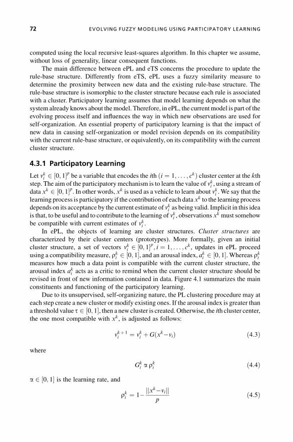
computed using the local recursive least-squares algorithm. In this chapter we assume,

without loss of generality, linear consequent functions.

The main difference between ePL and eTS concerns the procedure to update the

rule-base structure. Differently from eTS, ePL uses a fuzzy similarity measure to

determine the proximity between new data and the existing rule-base structure. The

rule-base structure is isomorphic to the cluster structure because each rule is associated

with a cluster. Participatory learning assumes that model learning depends on what the

system already knows about themodel. Therefore, in ePL, the currentmodel is part of the

evolving process itself and influences the way in which new observations are used for

self-organization. An essential property of participatory learning is that the impact of

new data in causing self-organization or model revision depends on its compatibility

with the current rule-base structure, or equivalently, on its compatibility with the current

cluster structure.

4.3.1 Participatory Learning

Let vki 2 0; 1½ �p be a variable that encodes the ith ði ¼ 1; . . . ; ckÞ cluster center at the kthstep. The aim of the participatorymechanism is to learn the value of vki , using a stream of

data xk 2 0; 1½ �p. In other words, xk is used as a vehicle to learn about vki . We say that the

learning process is participatory if the contribution of each data xk to the learning process

depends on its acceptance by the current estimate of vki as being valid. Implicit in this idea

is that, to be useful and to contribute to the learning of vki , observations xk must somehow

be compatible with current estimates of vki .

In ePL, the objects of learning are cluster structures. Cluster structures are

characterized by their cluster centers (prototypes). More formally, given an initial

cluster structure, a set of vectors vki 2 0; 1½ �p; i ¼ 1; . . . ; ck, updates in ePL proceed

using a compatibility measure, rki 2 ½0; 1�, and an arousal index, aki 2 ½0; 1�. Whereas rkimeasures how much a data point is compatible with the current cluster structure, the

arousal index aki acts as a critic to remind when the current cluster structure should be

revised in front of new information contained in data. Figure 4.1 summarizes the main

constituents and functioning of the participatory learning.

Due to its unsupervised, self-organizing nature, the PL clustering procedure may at

each step create a new cluster or modify existing ones. If the arousal index is greater than

a threshold value t 2 ½0; 1�, then a new cluster is created.Otherwise, the ith cluster center,

the one most compatible with xk, is adjusted as follows:

vkþ 1i ¼ vki þGðxk�viÞ ð4:3Þ

where

Gki a rki ð4:4Þ

a 2 ½0; 1� is the learning rate, and

rki ¼ 1� jjxk�vijjp

ð4:5Þ


with k:k a norm, p the dimension of input space, and

i ¼ arg maxjfrkj g ð4:6Þ

Notice that the ith cluster center is a convex combination of the new data sample xk

and the closest cluster center. Similarly to (4.3), the arousal index aki is updated as

follows:

akþ 1i ¼ aki þ bð1�rkþ 1

i �aki Þ ð4:7Þ

The value of b 2 ½0; 1� controls the rate of change of arousal: The closer b is to one,

the faster the system is to sense compatibility variations.

Theway in which ePL considers the arousal mechanism is to incorporate the arousal

index (4.7) into (4.4) as follows:

Gki ¼ aðrki Þ1�a

ki ð4:8Þ

When aki ¼ 0, we have Gki ¼ arki , which is the PL procedure with no arousal.

Notice that if the arousal index increases, the similarity measure has a reduced effect.

The arousal index can be interpreted as the complement of the confidencewe have in the

truth of the current belief, the rule-base structure. The arousal mechanism monitors the

performance of the system by observing the compatibility of the current model with

the observations. Therefore, learning is dynamic in the sense that (4.3) can be viewed as

a belief revision strategy whose effective learning rate (4.8) depends on the compat-

ibility between new data and the current cluster structure, and on model confidence

as well.

Figure 4.1. Participatory learning.


Notice also that the learning rate is modulated by compatibility. In conventional

learningmodels, there are no participatory considerations and the learning rate is usually

set small to avoid undesirable oscillations due to spurious values of data that are far from

cluster centers. Small values of learning rate, while protecting against the influence of

noisy data, slow down learning. Participatory learning allows the use of higher values of

learning rate; the compatibility index acts to lower the effective learning rate when large

deviations occur. On the contrary, when the compatibility is large, it increases the

effective rate, which means speeding up the learning process.

Clearly, whenever a cluster center is updated or a new cluster added, the PL fuzzy

clustering procedure should verify whether redundant clusters are created. This is

because updating a cluster center using (4.3) may push a given center closer to another

one and a redundant cluster may be formed. Therefore, a mechanism to exclude

redundancy is needed. One mechanism is to verify whether similar outputs due to

distinct rules are produced. In PL clustering, a cluster center is declared redundant

whenever its similarity with another center is greater than or equal to a threshold value\-

$\lambda$. If this is the case, then we can either maintain the original cluster center or

replace it with the average between the new data and the current cluster center. Similarly

to (4.5), the compatibility index among cluster centers is computed as follows:

rkvi ¼ 1�Xpj¼1jvki �vkj j ð4:9Þ

Therefore, if

rkvi � l ð4:10Þ

then the cluster i is declared redundant.

4.3.2 Parameter Estimation

After clustering, the fuzzy rule base is constructed using a procedure similar to eTS,

described in section 4.2. The cluster centers define the modal values of the Gaussian

membership functions while dispersions are chosen to achieve appropriate levels or rule

overlapping. Moreover, for each cluster found, the corresponding rules have their linear

consequent function parameters adjusted using the recursive least-squares algorithm.

The computational details are as follows.

Let xk ¼ bxk1 ; xk2 ; . . . ; xkpc½0; 1�p be the vector of observations and yki 2 ½0; 1� theoutput of the ith rule, i ¼ 1; . . . ; ck, at k ¼ 1, 2,. . .. Each local model is estimated by a

linear equation:

Yk ¼ Xkgk ð4:11Þ

where gk 2 Rpþ 1 is a vector of unknown parameters defined by

ðgkÞT ¼ gk0 gk1 g

k2 . . . gkp

h i


and Xk ¼ b1 xkc 2 ½0; 1�kðpþ 1Þthe matrix composed by the kth input vector xk and a

constant term; and Yk ¼ ½yki � 2 ½0; 1�k; i ¼ 1; . . . ; ck is the output vector.

Themodel (4.11) gives a local description of the system, but thevector of parameters

g is unknown. One way to estimate the values for g is to use the available data. Assume

that

Yk ¼ Xkgk þ ek ð4:12Þ

where gk represents the parameters to be recursively computed and ek is the modeling

error at k. The least-squares algorithm chooses gk to minimize sum-of-squares errors

Jk ¼ JðgkÞ ¼ ðekÞTek ð4:13Þ

Define Xkþ 1 and Ykþ 1 as follows:

Xkþ 1 ¼ Xk

1 xkþ 1

� �; Ykþ 1 ¼ Yk

ykþ 1i

� �ð4:14Þ

where xkþ 1 is the current input data and ykþ 1i is the corresponding model output.

The vector of parameters that minimizes the functional Jk at k is [32]:

gk ¼ Pkbk ð4:15Þ

where Pk½ðXkÞtXk��1 and bk ¼ ðXkÞTYk. Using the matrix inversion lemma [32]:

ðAþBCDÞ�1 ¼ A�1�A�1BðC�1þDA�1BÞ�1DA�1

and making

A ¼ ðPkÞ�1; C ¼ I; B ¼ Xkþ 1; D ¼ ðXkþ 1ÞT

we get

Pkþ 1 ¼ Pk I� Xkþ 1ðXkþ 1Þ�1Pk

1þðXkþ 1ÞTPkXkþ 1

" #ð4:16Þ

where I is the identity matrix. After simple mathematical transformations, the vector of

parameters is computed recursively as follows:

gkþ 1 ¼ gk þPkþ 1Xkþ 1 Ykþ 1�ðXkþ 1ÞTgk� � ð4:17Þ

Detailed derivation can be found in [10]. For convergence proofs see [16], for

example. Expression (4.17) is used to update the rule-consequent parameters at each k.


The use of the recursive least-squares algorithm depends on the initial values of the

parameters g0, and on the initial values of the entries ofmatrixP0. These initial values are

chosen based on the following:

1. Existence of previous knowledge about the system, exploring a database to find

an initial rule base, and, consequently, g0 and P0.

2. A useful technique when no previous information is available is to choose large

values for the entries of matrix P0 [29]. If the initial values of consequent

parameters are similar to exact values, then it is enough to choose small values for

the entries of P0. A standard choice of P0 is

P0 ¼ sIm

where Im is the identity matrix of the orderm, andm is the number of consequent

parameters. The value of s usually is chosen such that s2 [100,10000] if largevalues are required, while for the small values s2 [1,10]. More details can be

found in [29].

In this chapter, we use the first option; that is, we use a database to choose the

initial rule base and its parameters.

4.3.3 Evolving Fuzzy Participatory Learning Algorithm

The detailed steps of the evolving fuzzy participatory learning modeling procedure are

given by Algorithm 2.

Algorithm 2: ePL Procedure

Input: data samples, xk 2 ½0; 1�p; k ¼ 1; . . .

Output: model output

Initialize the rule focal points and parameters a; b; l; t:

1. Read new data xk.

2. Compute the compatibility index rki .3. Compute the arousal index aki :

if aki � t; 8i 2 f1; . . . ; ckgxk is a new cluster center; set ckþ 1 ¼ ck þ 1:

else compute (4.3) using (4.5)–(4.8)

4. Compute rkvi using (4.9):

if rkvi � lexclude viset ckþ 1 ¼ ck�1:

5. Update rule-base structure.

6. Compute rules-consequent parameters.

7. Compute firing degree using (4.1).

8. Compute output using (4.2).


Detailed guidelines to choose appropriate values of a, b, l, and t are given in [21],where it is shown that they should be chosen such that:

0 <tb� 1�l � 1

where t � b and l � 1�t. These steps are shown in Figure 4.2.

update rule base

compute firing degree

compute model output

no

similarity

greater than

threshold

yes eliminate

similar center

update most

compatible cluster center

compute similarity

index of cluster centers

no

create new cluster

with center at the

current data

yes

read data

compute

arousal index

arousal

greater than

threshold

compute

compatibility index

Figure 4.2. Computational steps of ePL.


4.4 EXPERIMENTS WITH A BENCHMARK PROBLEM

In this section, the ePL model is used to model and predict the future values of the gas

furnace Box & Jenkins time series. The Box & Jenkins gas furnace is a well-studied

benchmark problem in the literature. It is composed of 290 pairs of input–output data

taken from a laboratory furnace [12], emerging from a data set composed of a total 296

values. Each data sample consists of themethane flow rate, the process input variable, uk,

and the CO2 concentration in off gas, the process output yk. This is a dynamic process

with one input uk and one output yk. The aim is to predict current output yk using past

input and output values, with the lowest error. Different studies indicate that the best

model structure for this system is:

yk ¼ f b yk�1; uk�4c ð4:18Þwhere yk is the model output. We consider the following case: 200 training data

examples to initialize the fuzzy rule base and the remaining 90 data pairs to test and

validate.

Model evaluation is performed considering the root mean square error (RMSE) and

the nondimensional error index (NDEI), which is the ratio between the RMSE and the

standard deviation of the target data. These indexes are computed using the following

expressions:

RMSE ¼ 1

N

XNk¼1ðdk�ykÞ2

!1=2

ð4:19Þ

NDEI ¼ RMSE

stdðdkÞ ð4:20Þ

whereN is the number of predictions; yk, themodel output, is the desired output; and dk is

the desired output and std is the standard deviation function.

Comparison of the ePL model against neural/neuro-fuzzy approaches and evolving

models is summarized in Table 4.1. Figure 4.3 shows the actual and forecasted values

provided by the ePL model.

T A B L E 4.1. Modeling Performance for the Box & Jenkins Benchmark

Model Name and Source Number of Rules (or Nodes) RMSE NDEI

MLP model [27] 5 0.0211 0.1319

ANFIS model [14] 7 0.0207 0.1294

FuNN model [18] 7 0.0226 0.1408

HyFIS model [20] 15 0.0205 0.1278

eTS model [4] 5 0.0490 0.3057

Simpl_eTS model [4] 3 0.0485 0.3023

xTS model [8] 6 0.0375 0.2397

ePL current model 4 0.0191 0.1189


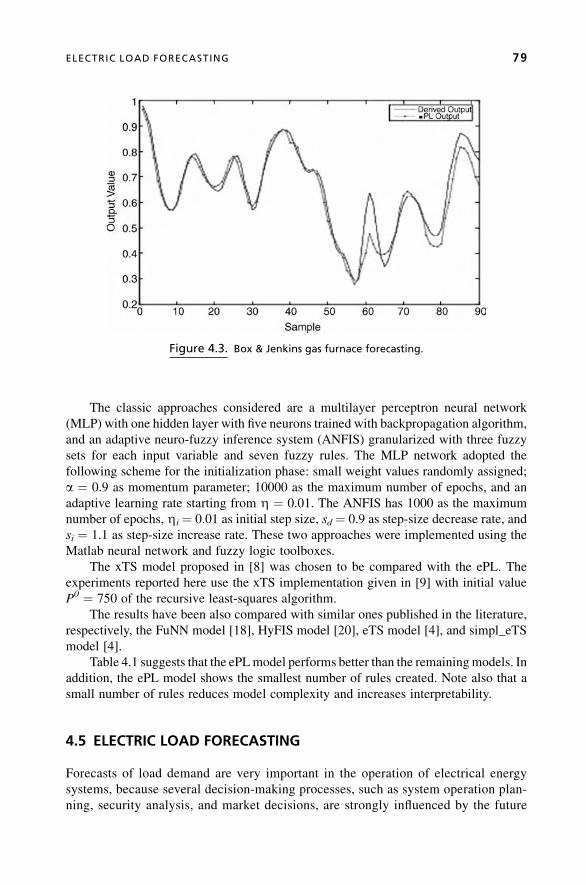
The classic approaches considered are a multilayer perceptron neural network

(MLP) with one hidden layer with five neurons trained with backpropagation algorithm,

and an adaptive neuro-fuzzy inference system (ANFIS) granularized with three fuzzy

sets for each input variable and seven fuzzy rules. The MLP network adopted the

following scheme for the initialization phase: small weight values randomly assigned;

a ¼ 0.9 as momentum parameter; 10000 as the maximum number of epochs, and an

adaptive learning rate starting from Z ¼ 0.01. The ANFIS has 1000 as the maximum

number of epochs, Zi ¼ 0.01 as initial step size, sd ¼ 0.9 as step-size decrease rate, and

si ¼ 1.1 as step-size increase rate. These two approaches were implemented using the

Matlab neural network and fuzzy logic toolboxes.

The xTS model proposed in [8] was chosen to be compared with the ePL. The

experiments reported here use the xTS implementation given in [9] with initial value

P0 ¼ 750 of the recursive least-squares algorithm.

The results have been also compared with similar ones published in the literature,

respectively, the FuNN model [18], HyFIS model [20], eTS model [4], and simpl_eTS

model [4].

Table 4.1 suggests that the ePLmodel performs better than the remainingmodels. In

addition, the ePL model shows the smallest number of rules created. Note also that a

small number of rules reduces model complexity and increases interpretability.

4.5 ELECTRIC LOAD FORECASTING

Forecasts of load demand are very important in the operation of electrical energy

systems, because several decision-making processes, such as system operation plan-

ning, security analysis, and market decisions, are strongly influenced by the future

Figure 4.3. Box & Jenkins gas furnace forecasting.

ELECTRIC LOAD FORECASTING 79

values of the load. In this context, a significant error in the load forecast may result in

economic losses, security constraints violations, and system operation drawbacks.

Accurate and reliable load forecasting models are essential for a suitable system

operation.

The problem of load forecasting can be classified as long, medium, and short term,

depending on the situation. Long-term forecasting is important for capacity expansion of

the electrical system. Medium term is important to organize the fuel supply, in

maintaining operations, and in interchange scheduling. Short-term forecasting is gen-

erally used for daily programming and operation of the electrical system, energy transfer,

and demand management [26].

Particularly in the context of short-term hydrothermal scheduling, load forecasting

is important to elaborate the next-day operation scheduling because errors in load

forecasting can cause serious consequences, affecting the efficiency and the safety of the

system (cost increasing, insufficient electrical energy supply to the existing demand).

The goal of short-term load forecasting is to accurately predict the 24 hourly loads of

the next operation day, one-step-ahead. The effectiveness of the ePL approach is

illustrated using load data of a major electrical utility located in the Southeast region

of Brazil. In evaluating the forecast model, a database consisting of hourly loads from

August 1, 2000 to August 31, 2000 is used to develop the model and to produce load

forecasts.

Forecasting performance requires an appropriate selection of the input variables

of the forecasting model. Here, the number of inputs was found using the partial

autocorrelation function. Figure 4.4 shows the first 36 estimated partial autocorrelations

Figure 4.4. Estimated partial autocorrelation function and standard error limits.


of the series. The behavior of the function suggests two inputs, respectively, yt to forecast

yt�2, yt�1. The points between the two dotted lines of Figure 4.4 are within two standarddeviations of the estimated partial autocorrelation.

The performance of the ePL is compared with MLP, ANFIS, eTS, and xTS models.

The models were developed to forecast hourly loads during the 24-hour period of

August 31, 2000. Themodelswere developd using data fromAugust 1, 2000 until August

30, 2000. Data were normalized to fit the unit interval as follows:

yt ¼ zt�min

max�min

where yt is the normalized data, and min and max denote the minimum and maximum

values of zt; t ¼ 1; . . . ;N.The performance of the forecasting models was evaluated using the root mean

square error (RMSE) (4.19) and the nondimensional error index (NDEI) (4.20).

The ePL model adopted the following values: b ¼ t ¼ 0:30, r ¼ 0:25, and

l ¼ 0:35. These are the only parameters of the ePL algorithm that need to be chosen

by the user. The ePL found five rules during the 30-day development period. During

testing, ePL uses hourly loads data and runs as in online mode.

An MLP with the same structure and initial parameters as that developed for

the Box & Jenkins benchmark was used to forecast loads in the period. MLP training

also started with small, randomly chosen initial weights and took 5000 epochs to

converge.

Load forecasting for the same time period also has been done using ANFIS. The

structure and parameters are also the same those used for the Box& Jenkins problem, and

the maximum number of epochs was 1000.

The eTS and xTS models were developed considering the first 30 days before

the testing period. The value of the cluster radii for the eTS model was r ¼ 0.4.

Both eTS and xTS models adopted P0 ¼ 750 to initialize the recursive least squares.

In the experiments reported here, we ran the eTS and xTS implementation given

in [9].

Table 4.2 shows the performance of the models during the testing period (24 hours),

considering the two error criteria (4.19) and (4.20). The table also includes the final

T A B L E 4.2. Modeling Performance for One-Step-Ahead Load Forecast

Model Name and Source Number of Rules (or Nodes) RMSE NDEI

MLP model [27] 5 0.0522 0.2055

ANFIS model [14] 9 0.0541 0.2012

eTS model [4] 6 0.0517 0.1922

xTS model [8] 4 0.0562 0.2089

ePL current model 5 0.0508 0.1888

ELECTRIC LOAD FORECASTING 81

number of fuzzy rules (or nodes) achieved by models. Load forecasts are shown in

Figures 4.5–4.9.

Notice in Table 4.2 that the ePL approach gives as good results as eTS and xTS, but is

simpler and computationally more efficient than eTS and xTS.

Figure 4.6. Load forecast for August 31, 2000—ANFIS.

Figure 4.5. Load forecast for August 31, 2000—MLP.


4.6 CONCLUSION

This chapter addressed evolving fuzzy participatory learning, a method based on the

participatory learning paradigm to develop evolving fuzzy rule-based models. Partici-

patory learning materializes in the evolving fuzzy participatory method in the form of an

Figure 4.8. Load forecast for August 31, 2000—xTS.

Figure 4.7. Load forecast for August 31, 2000—eTS.

CONCLUSION 83

unsupervised clustering algorithm. Clustering is a key issue in evolving fuzzy systems

because they must dynamically find an appropriate structure in a stream of data.

Unsupervised dynamic clustering provides an efficient mechanism to implement a form

of self-organization in system modeling. Similarly to eTS, parameters of rule conse-

quents are computed using the least-squares algorithm. Computational experiments with

a classic benchmark problem and a real-world application concerning hourly electrical

load forecasting show that ePL is a promising approach in the adaptive fuzzy systems

modeling area.

4.7 ACKNOWLEDGMENTS

This work was supported by the Research Foundation of the State of Sao Paulo

(FAPESP), grants 03/10019-9, 05/58879-1 and 03/05042-1; and by the Brazilian

National Research Council (CNPq), grants 305796/2005-4 and 304857/2006-8. The

authors also thank Plamen Angelov and the anonymous referees for comments that

helped us to improve the chapter.

4.8 REFERENCES

1. K. L. Anderson, G. L. Blackenship, L. G. Lebow, “A Rule-Based Adaptive PID Controller.”

Proc. 27th IEEE Conf. Decision Control, New York, 1988, pp. 564–569.

2. P. Angelov, Evolving Rule-Based Models: A Tool for Design of Flexible Adaptive Systems.

Heidelberg, New York; Springer-Verlag, 2002, ISBN 3-7908-1457-1.

Figure 4.9. Load forecast for August 31, 2000—ePL.


3. P. Angelov, D. Filev. “An Approach to On-line Identification of Evolving Takagi-Sugeno

FuzzyModels.” IEEETrans. on Systems,Man andCybernetics, part B, 34 (1): 484–498, 2004.

4. P.Angelov,D. Filev. “Simpl_eTS:ASimplifiedMethod forLearningEvolvingTakagi-Sugeno

Fuzzy Models.” Proc. 2005 Int. Conf. on Fuzzy Systems, FUZZ-IEEE, May 2005,

pp. 1068–1073.

5. P. Angelov, R.Guthke, “AGA-BasedApproach toOptimization ofBioprocessesDescribed by

Fuzzy Rules,” Journal Bioprocess Engineering, 16: 299–301, 1997.

6. P. Angelov, N. Kasabov, “Evolving Intelligent Systems—eIS.” IEEE SMC NewsLetter, June

2006, pp. 1–13.

7. P. Angelov, C. Xydeas, D. Filev, “On-line Identification of MIMO Evolving Takagi-Sugeno

Fuzzy Models.” Int. Joint Conference on Neural Networks and International Conference on

Fuzzy Systems, Budapest, Hungary, July 2004, IJCNN-FUZZ-IEEE, pp. 55–60.

8. P. Angelov, X. Zhou, “Evolving Fuzzy Systems from Data Streams in Real-Time.” Proc. Int.

Symposium on Evolving Fuzzy Systems, 2006, pp. 29–35.

9. P. Angelov, X. Zhou,“Online Identification of Takagi-Sugeno Fuzzy Models DeMO,” 2006,

http://194.80.34.45/eTS/.

10. K. J. Astrom, B. Wittenmark. Adaptive Control, 2nd ed. Boston: Addison-Wesley-Longman,

1994.

11. R. Babuska, Fuzzy Modeling for Control. Boston: Kluwer Academic Publishers, 1998.

12. G. E. P. Box, G. M. Jenkins, Time Series Analysis—Forecasting and Control, 2nd ed. Holden

Day, CA, 1976.

13. S. L. Chiu, “FuzzyModel Identification Based on Cluster Estimation,” Journal of Intelligence

and Fuzzy System, 2: 267–278, 1994.

14. J. S. R. Jang, “ANFIS: Adaptative Network-Based Fuzzy Inference Systems.” IEEE Trans. on

Systems, Man and Cybernetics, 23: 665–685, June 1993.

15. T. A. Johanson, R. Murray-Smith, “Operating Regime Approach to Nonlinear Modeling and

Control.” InMultiple Model Approaches to Modeling and Control, ( R. Murray-Smith, T. A.

Johanson, eds.). Hants, UK: Taylor Francis, 1998, pp. 3–72.

16. C. R. Johnson, Lectures and Adaptive Parameter Estimation. Upper Saddle River, NJ:

Prentice-Hall, 1988.

17. N. Kasabov, Evolving Connectionist Systems: Methods and Applications in Bioinformatics,

Brain Study and Intelligent Machines. London: Springer-Verlag, 2002.

18. N. Kasabov, J. Kim, M.Watts, A. Gray, “FuNN/2—A Fuzzy Neural Network Architecture for

Adaptive Learning and Knowledge Acquisition,” Information Sciences, 3–4 (101): 155–175,

October 1997.

19. N. Kasabov, Q. Song, “DENFIS: Dynamic Evolving Neural-Fuzzy Inference System and Its

Application for Time Series Prediction.” IEEE Trans. on Fuzzy Systems, 10 (2): 144–154,

2002.

20. J. Kim,N.Kasabov, “HyFIS: AdaptiveNeuro-Fuzzy Inference Systems andTheir Application

to Nonlinear Dynamical Systems,” Neural Networks, 12: 1301–1319, June 1999.

21. E. Lima, “Modelo Takagi-Sugeno Evolutivo Participativo,” PhD thesis, Faculty of Electrical

and Computer Engineering, State University of Campinas, 2008.

22. F. J. Lin, C. H. Ln, P. H. Shen, Self-Constructing Fuzzy Neural Network Speed Controller for

Permanent-Magnet SynchronousMotorDrive. IEEETrans. on Fuzzy Systems, 5(9): 751–759,

2001.

REFERENCES 85

23. O. Nelles, Nonlinear System Identification. Heidelberg: Springer, 2001.

24. F. Hoffmann, L. Magdalena, O. Cordon, F. Herrera. Generic Fuzzy Systems: Evolutionary

Tuning and Learning of Fuzzy Knowledge Bases. Singapore: World Scientific Publishing,

2001.

25. W. Pedrycz, F. Gomide, Fuzzy Systems Engineering: Toward Human-Centric Computing.

Hoboken, NJ: Wiley Interscience/IEEE, 2007.

26. S. Rahman, O. Hazim, “A Generalized Knowledge-Based Short-Term Load-Forecasting

Technique.” IEEE Trans. on Power Systems, 8 (2), 1993.

27. D. Rumelhart, G. Hinton, R. Williams, Learning Internal Representation by Error Propa-

gation. London: Nature, 1986.

28. L. Silva, F.Gomide, R. R.Yager, “Participatory Learning in FuzzyClustering.” 2005 IEEE Int.

Conf. on Fuzzy Systems, May 2005, FUZZ-IEEE, pp. 857–861.

29. P. E. Wellstead, M. B. Zarrop, Self-Tuning Systems: Control and Signal Processing. New

York: John Wiley & Sons, 1995.

30. R. Yager, D. Filev, “Approximate Clustering via the Mountain Method.” IEEE Trans. on

Systems, Man and Cybernetics, 24 (8): 1279–1284, August 1994.

31. R. R. Yager, “A Model of Participatory Learning.” IEEE Trans. on Systems, Man and

Cybernetics, 20: 1229–1234, 1990.

32. P. C. Young, Recursive Estimation and Time-Series Analysis. Berlin: Springer-Verlag, 1984.


5

TOWARD ROBUST EVOLVINGFUZZY SYSTEMS

Edwin Lughofer

Abstract: In this chapter, methodologies for more robustness and transparency in

evolving fuzzy systems will be demonstrated. After outlining the evolving fuzzy

modeling approaches, FLEXFIS (FLEXible Fuzzy Inference Systems) for fuzzy

regression models and FLEXFIS-Class (FLEXible Fuzzy Inference Systems

for Classification) for fuzzy classification models, robustness improvement strategies

during the incremental learning phase will be explained, including regularization issues

for overcoming instabilities in the parameter estimation process, overcoming the

unlearning effect, dealing with drifts in data streams, ensuring a better extrapolation

behavior, and adaptive local error bars serving as local confidence regions surrounding

the evolved fuzzymodels. The chapter will be concludedwith evaluation results on high-

dimensional real-world data sets, where the impact of the new methodologies will be

presented.

5.1 INTRODUCTION

5.1.1 Purpose of Robust Evolving Models

Nowadays, automatic adaptation techniques and evolving schemes for data-driven

models, that is, models that are fully built up from data, measurement data, or online


and Nikola Kasabov


data streams, are becomingmore andmore an essential point in industry. Today’s quality

control systems need to achieve high accuracies when doing clustering respectively,

grouping of data, prediction of future system states, or system identification, or when

classifying new production items. For instance, in a fault detection or decision support

system a hit rate of 95% or even higher is required; otherwise the throughput of broken

items or wrongly classified objects would raise significant customer complaints or may

even lead to failures in the system, and finally to severe breakdowns of components in a

system or the whole production cycle.

A large amount of samples is needed to set up an initial model framework in offline

mode that should achieve a high accuracy and guarantee a safe production. This is

because usually not all possible operating conditions can be covered by offline simulated

or recorded data in advance; sometimes, a completely new system behaviormay demand

feedback from a model in its extrapolation space, which is always quite precarious

and risky to follow. It is thus a requirement that the models are refined, extended, and

evolved online during normal production. Now, the amount of data and the cycle times

for such processes usually do not allow postprocessing of batches of data. Consequently,

this is an online processing of tasks, which requires an update of some components of

the models in the form of incremental learning steps with new data (i.e., the models

are evolved sample per sample). An alternative complete rebuilding of the models from

time to timewith all the data samples, recorded online so far,would yield an unacceptable

computational effort as not terminating in real-time.

One important aspect when doing evolving modeling is to guarantee a robust

learning behavior in order to assure models with high prediction, classification, and

control performance. Hereby we see two basic aspects for assuring robustness during

online learning and high-performance models:

1. Doing incremental and evolving learning in a way such that the performance of

the evolved models is close to the (hypothetical) batch solution (achieved by

collecting all the data and loading them at once into the training algorithm). From

a mathematical point of view, this means that a kind of convergence of some

parameters to an optimality criterion is achieved.

2. Implementing approaches for assuring high performance of the models with

respect to accuracy and correctness also in specific cases such as (a) instabilities

during parameter estimation, (b) situations causing an unlearning effect, (c) drifts

in online data streams, (d) extrapolation situations for new samples to be

predicted (i.e., new data samples to be classified appearing outside the previously

estimated feature space), and (e) uncertainties in the models due to high noise

levels. These approaches include (a) regularization, (b) a strategy for when to

update, (c) detection of drifts and gradual forgetting, (d) avoidance of a

reactivation of inner fuzzy sets, and (e) adaptive local error bars serving as

confidence regions surrounding the evolved models and hence delivering a kind

of plausibility criterion of the models’ decisions.

Both definitions of robustness will be addressed in subsequent sections for a

specific type of model architecture: evolving fuzzy systems.

88 TOWARD ROBUST EVOLVING FUZZY SYSTEMS

5.1.2 Fuzzy Systems

Fuzzy systems play an important role for the automatization of modeling, identification,

and classification tasks, as they usually represent a good tradeoff between models with

high accuracy and linguistic interpretability and transparency [12, 30]. The latter is

because their architecture contains rule bases and therefore may yield a better under-

standing of some underlying system behaviors than pure black-box models (such as

neural networks [25]). Transparency and linguistic interpretability can be used, for

instance, for fault analysis and reasoning [28] to trace back faults in the system and find

the reasons for them. Another important aspect in modeling is the mimicry of human

imprecision and vague knowledge. This can be easily achieved with fuzzy systems,

as the inner structure of these yields quite a good direct representation of vague

knowledge (in form of rules). They are often applied in areas such as system identi-

fication [31] and analysis, control [1, 7], fault detection [44], novelty detection [17], or

classification [48].

5.1.3 Evolving Fuzzy Systems for Regression

In order to cope with the online demands mentioned in the previous section, various

approaches for evolving fuzzy and neuro-fuzzy systems were developed in the past

decade, such as eTS [5] and the simplified version Simp_eTS [2] for rule-base simpli-

fication,DENFIS [33, 34], online SOFNN [36], SAFIS [21], participatory evolving fuzzy

modeling [38], DFNN [63] and its successor GDFNN [64] or the approach presented

in [8].

eTS [5] exploits a Takagi-Sugeno fuzzy model and recursively updates the structure

of the model based on the potential of the input data (i.e., it implements a kind of

incremental version of subtractive clustering). A new rule is added when the potential of

the data is higher than the potential of the existing rules or a new rule ismodifiedwhen the

potential of the new data is higher than the potential of the existing rules and the new data

are close to an old rule. Its simplified version, Simp_eTS [2] extends eTS [5] by including

an online rule-base simplification algorithm based on the population of the rules,

determined as the number of data samples belonging to the corresponding clusters. In

DENFIS [34] the structure learning is carried out with the help of an evolving clustering

method, called ECM [32]; that is, whenever a new cluster is found, automatically a new

rule is set as well. The antecedent fuzzy sets with fixedwidth for each dimension are then

formed around the corresponding center coordinates and the linear consequent para-

meters are estimated by a recursive weighted least-squares estimator. SAFIS [21] as a

truly sequential learning algorithm uses the idea of functional equivalence between an

RBF neural network and a fuzzy inference system by the application of the GAP-RBF

neural network proposed by [27]. In online SOFNN [36] the learning is divided into a

parameter and a structure learning; the former exploits a modified version of recursive

least squares [39] and the structure learning includes new adding and pruning techniques.

The adding approach is derived from geometric growing criterion and satisfies the

[epsilon]-completeness of fuzzy rules [35]. Participatory evolving fuzzy modeling [38]

combines the concept of participatory learning (PL) introduced by Yager [66] with the

INTRODUCTION 89

evolving fuzzy modeling approach eTS [5] (by Angelov & Filev). The PL concept is

based on unsupervised clustering and hence is a natural candidate to find rule-base

structures in adaptive fuzzy modeling procedures. Another variant is the FLEXFIS

approach [41] (FLEXible Fuzzy Inference Systems), which exploits an evolving version

of vector quantization [40] including an alternativewinner selection strategy and a split-

and-merge procedure for rule evolution and antecedent update, which is connected with

recursive weighted least squares for local learning of rule consequents (achieving a high

flexibility and convergence of the consequent parameters).

5.1.4 Evolving Fuzzy Systems for Classification

For classification tasks in online systems, incremental learning approaches for fuzzy

classifiers were developed, such as [58, 60]. In the latter an incremental learning

technique for classical fuzzy classification model architecture [48, 52] is demonstrated,

which approximates the regions belonging to different classes with multidimensional

rectangles, and a new rule (hidden neuron) is generated whenever a sample is mis-

classified or not covered by any rule at all. Probably the most famous approach is an

evolving fuzzy classifier family called eClass [4], which comes with three model

architectures [3] (classical single-model architecture with class label in the consequent,

single and first-order TSK-type classifier with single and multiple consequents) and is

able to evolve new rules and prune older rules (clusters) on demand based on a recursive

online calculation of potentials of cluster prototypes and input data. Another variant of

this evolving fuzzy classifier is the FLEXFIS-Class approach (FLEXible Fuzzy Infer-

ence Systems for Classification) [42], which comes with two model architectures, again

classical single-model architecture with class label in the consequent (FLEXFIS-Class

SM) and an architecture based on multiple first-order TSK fuzzy models (FLEXFIS-

Class MM). The latter evolves separate first-order TSK fuzzy regression models (one for

each class) with the usage of FLEXFIS based on indicator vectors and applies a one-

versus-rest classification scheme.

5.1.5 Structure of the Chapter

In this chapter, we first give a short summary of the principal techniques and algorithms

of FLEXFIS [41], applicable for online regression problems, as well as FLEXFIS-

Class [42], applicable for building up an evolving fuzzy classifier for online classification

problems. The major novel contribution of this chapter lies in the second part, wherewe

focus on issues guiding the evolving learning algorithms tomore robustness and stability

during the learning process and hence achieving higher performance of the evolved

models (see also previous section). These issues are indeed implemented in FLEXFIS

and respectively FLEXFIS-Class (hence a short summary of these methods and

references where appropriate is given beforehand in order to keep the chapter self-

contained), but are generically described in the sense that they can be quite easily adopted

for most of the evolving fuzzy systems and classifiers approaches mentioned above.

Evaluation of the proposed approaches will be done throughout the whole chapter, both


on two-dimensional simple examples for visualization to the reader and on higher-

dimensional problems from real-world applications (section 5.5).

5.2 EVOLVING FUZZY REGRESSION MODELS WITH FLEXFIS

We outline the most important characteristics of the basic FLEXFIS method (for further

details see [41]) and mention a stepwise description of the algorithm.

The characteristics of this evolving fuzzymodeling variant can be summarized in the

following points:

. It applies an extension of conventional vector quantization (VQ) [18] by incor-

porating a vigilance parameter, which steers the tradeoff between plasticity and

stability during incremental online learning. Plasticity is the ability to adapt to

new information, whereas stability is the ability to converge to an optimal

solution. This is motivated in the adaptive resonance theory network (ART)

approach [11] and is exploited for forming a one-pass incremental and evolving

clustering process, called evolving vector quantization (eVQ) [40]. When doing

so, it connects a cluster evolution condition and an alternative distance strategy for

samplewise winner selection, which is based on the distance calculation to the

surface rather than to the centers (as done in conventional VQ). Hence the surface

is calculated incrementally synchronously to the centers.

. Each cluster stands for one rule and the clusters are projected onto the axes in order

to form the Gaussian fuzzy sets and the antecedent parts of the rules.

. It uses recursive local learning by exploiting recursive weighted least squares [39]

for the linear consequent parameters in a fuzzy basis function network introduced

in [61], that is, a Takagi-Sugeno fuzzy system with Gaussian fuzzy sets and

product t-norm as conjunction operator, in the case of C rules defined as:

f fuzð~xÞ ¼ yfuz ¼XCi¼1

lið~xÞYið~xÞ ð5:1Þ

with the normalized membership functions

Yið~xÞ ¼ mi

ð~xÞXCj¼1

mjð~xÞð5:2Þ

and mi as rule fulfillment of the ith rule

mið~xÞ ¼ exp � 1

2

Xpj¼1

ðxj�cijÞ2s2ij

!ð5:3Þ

EVOLVING FUZZY REGRESSION MODELS WITH FLEXFIS 91

and consequent functions

lið~xÞ ¼ wi0þwi1x1þwi2x2þ . . . þwipxp ð5:4Þ

where cij is the center and sij is the width of the Gaussian function appearing as a

fuzzy set in the jth antecedent part (i.e., the antecedent part for the jth input

dimension) of the ith rule. In this sense, local linear models li are connected

through an inference scheme, where the Gaussian functions serve as kernel

functions and weight new incoming samples according to their distance to the

centers. One major advantage is that with a local learning technique the conse-

quent parameters~w of each rule can be incrementally trained separately and hence

an evolution of a new rule does not disturb the consequent parameter training of the

others [5]; this is for more flexibility during the training process. Another major

advantage of local learning is that the hyperplanes describing the consequent

functions tend to snuggle along the surface [45], which is also the key condition for

obtaining reliable local error bars as outlined in section 5.4.5.

. It connects two previous learning issues by taking care that a near-optimal solution

is reached that is close to the optimal one in the least-squares sense (deviating from

the optimal one by a small constant). This can be shown analytically and

empirically; for details see [41].

The final point in the itemization addresses the problem of robustness as outlined in

section 5.1. (first itemization point). In fact, correction terms are integrated in the

learning procedure, which balance out the nonoptimal situation, appearing during the

training process as clusters; hence, rules are shifted and moved. Therefore, the recursive

weighed least-squares approach, whichwould guide the parameter solution to optimality

in case of fixed premise parts, is disturbed. The correction terms cannot be calculated in

an incremental fashion, but it can be shown that they are forced to a decreasing sequence,

leading to a near-optimal solution (for details see [41]). This is achieved on the basis that

clusters are forced to evolve into a balanced state. The balanced state is guaranteed by

controlling the tradeoff between plasticity (ability to adapt to new information) and

stability (ability to converge to an optimal solution) with a vigilance parameter: If, for

instance, two different main states occur during the online process, two different clusters

will evolve automatically in the eVQ process; this will prevent strong fluctuating

movements of one cluster, as the cluster centers and surfaces are always adapted within

local areas.

Figure 5.1 shows an empirical justification of this point by the dependency of

model qualities (maximum quality¼ 1) on the number of data samples each block

contains loaded into FLEXFIS. This is done for a practical application example, where

32 different models are trained based on (noisy) measurement data from engine test

benches and their average model quality is measured in terms of the average r-squared-

adjusted measure [23], punishing more complex models by dividing r-squared

measures with the number of model parameters. The maximum of 960 data samples

denotes the whole batch of data collected, and FLEXFIS applied on it in batch mode

(complete antecedent learning first and complete consequent estimation afterward)


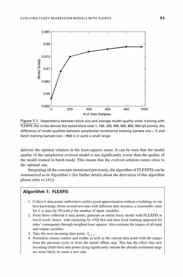
delivers the optimal solution in the least-squares sense. It can be seen that the model

quality of the samplewise evolved model is not significantly worse than the quality of

the model trained in batch mode. This means that the evolved solution comes close to

the optimal one.

Integrating all the concepts mentioned previously, the algorithm of FLEXFIS can be

summarized as in Algorithm 1 (for further details about the derivation of this algorithm

please refer to [41]).

Algorithm 1: FLEXFIS

1. Collect k data points sufficient to yield a good approximation without overfitting; to our

best knowledge (from several test-runs with different data streams), a reasonable value

for k is maxð4p; 50Þwith p the number of input variables.

2. From these collected k data points, generate an initial fuzzy model with FLEXFIS in

batch mode, hence, with clustering by eVQ first and then local learning approach for

rules’ consequents through weighted least squares. Also estimate the ranges of all input

and output variables.

3. Take the next incoming data point: ~xkþ 1.

4. Normalize cluster centers and widths as well as the current data point with the ranges

from the previous cycle or from the initial offline step. This has the effect that new

incoming (fault-free) data points lying significantly outside the already-estimated range

are more likely to cause a new rule.

Figure 5.1. Dependency between block size and average model quality when training with

FLEXFIS; the circles denote the tested block sizes 1, 100, 200, 400, 600, 800, 960 (all points); the

difference of model qualities between samplewise incremental training (sample size¼ 1) and

batch training (sample size¼960) is in quite a small range.

EVOLVING FUZZY REGRESSION MODELS WITH FLEXFIS 93

5. If the current data point lies inside any cluster’s range of influence:

(a) Calculate the distance of the selected data point to all those cluster centers belonging

to clusters the new sample lies inside by using Euclidian distance measure.

(b) Elicit the cluster center that is closest to the data point by taking theminimumover all

calculated distances ! winner cluster cwin.

(c) Set mindist ¼ 0 (this forces the algorithm that no new cluster is generated).

6. Else If the current data point lies outside of all clusters’ range of influence:

(a) Calculate the distance of ~x to the surface of all clusters.

(b) Elicit the cluster center that is closest to the data point by taking theminimumover all

calculated distances ! winner cluster cwin.

(c) Set mindist as the minimum over all distances.

7. If mindist � r:(a) Increase the number of clusters from C to Cþ 1.

(b) Start a new cluster at the kþ 1th point, hence,~cC ¼~xkþ 1 with c the center of the new

cluster.

(c) Set the width of the new cluster to zero, hence, ~sC ¼~0.(d) Transfer cluster centers and widths back to original range.

(e) Project the new cluster to the axes to from the antecedent part (fuzzy sets) of the new

rule; hereby set thewidth of the fuzzy set in the ith dimension to e*rangeðxiÞwith e asmall value.

(f) Set the linear consequent parameter ~wC of the new rule to~0.(g) Set the inverse covariance matrix PC of the new rule to aI.

8. ELSE:

(a) Update the p center components of the winner cluster cwin by cwinðnewÞ ¼cwinðoldÞþhwinð~xkþ 1�cwinðoldÞÞ with the choice of an adaptive learning gain

hwin ¼ 0:5kwin

with kwin the number of data samples forming the winning cluster.

(b) Update the pwidth components ofwinner cluster cwin by using the recursive variance

update formula [51].

(c) Transfer cluster centers and widths back to original range.

(d) Project winner cluster onto the axes to update the antecedent part of the rule

belonging to the winner cluster; assure that the width of the fuzzy set in the ith

dimension is equal or bigger than e*rangeðxiÞ.(e) Correct the linear parameter vector of consequent functions and the inverse

covariance matrix of the rule corresponding to the winning cluster:

~wwinðkÞ ¼ ~wwinðkÞþ~dwinðkÞ PwinðkÞ ¼ PwinðkÞþDwinðkÞ ð5:5Þ

9. Perform recursive weighted least squares for the consequent parameters in all

i ¼ 1; . . . ;C rules by

~wiðkþ 1Þ ¼ ~wiðkÞþ gðkÞðyðkþ 1Þ�~rTðkþ 1Þ~wiðkÞÞ ð5:6Þ

gðkÞ ¼ Piðkþ 1Þ~rðkþ 1Þ ¼ PiðkÞ ~rðkþ 1Þ1

Yið~xðkþ 1ÞÞ þ~rTðkþ 1ÞPiðkÞ~rðkþ 1Þ ð5:7Þ

Piðkþ 1Þ ¼ ðI�gðkÞ~rTðkþ 1ÞÞPiðkÞ ð5:8Þ


with Yið~xðkþ 1ÞÞ the normalized membership function value for the ðkþ 1Þthdata sample as weight in the update process, PiðkÞ the weighted inverse covariance

matrix, and~rðkþ 1Þ ¼ ½1x1ðkþ 1Þx2ðkþ 1Þ . . . xpðkþ 1Þ�T the regressor values of the

ðkþ 1Þth data point, which is the same for all C rules.

10. Update the ranges of all input and output variables.

11. If new data points are processed, set k ¼ kþ 1 and GOTO Step 3, ELSE stop.

From this algorithm it is clear that an initial training phase has to take place. At first

glance, this seems to be a drawback versus other approaches that are able to perform

incremental learning from the start. However, it should be emphasized that in industrial

applications usually an offline modeling step is required in order to get a feeling of the

performance of the models and to be able to carry out an analysis of some model

components (for examining reliability and reasonability). Furthermore, an initial model

building (which is also possible during online modewhen carried out on just the first few

dozen samples) delivers a good first guess of an appropriate setting of the most important

parameter (the vigilance r, which guides the number of rules) in FLEXFIS, especially

when applied within a best parameter grid search procedure connected with a cross-

validation process (see also section 5.5).

5.3 EVOLVING FUZZY CLASSIFIERS WITH FLEXFIS-CLASS

FLEXFIS-Class [42] exploits two model architectures:

1. Single-model architecture (usually called the classical fuzzy classifier architec-

ture [29, 46, 48, 52]) whose rules are defined in the following way:

Rulei : IF x1 IS mi1 AND . . .AND xp IS mip THEN yi ¼ Li

ð5:9Þ

where p is the dimensionality of the input space, mi1; . . . ;mip are the p antecedent

fuzzy sets, and Li is the crisp output class label from the set f1; . . . ;KgwithK the

number of classes. When classifying a new sample~x, the final crisp class label isobtained by taking the class label of the rule with the highest activation degree,

that is, by calculating

y ¼ Li� with i� ¼ argmax1�i�R ti ð5:10Þ

with R the number of rules and ti the activation degree of rule i defined by a t-

norm that is usually expressed as a product operator [65]:

ti ¼ Tp

j¼1mijðxjÞ

EVOLVING FUZZY CLASSIFIERS WITH FLEXFIS-CLASS 95

where mij are the membership functions of the antecedent fuzzy sets defined by a

Gaussian:

mij ¼ e�1

2

ðxj�cij Þ2s2ij ð5:11Þ

with cij signifying the centers and sij the spread of the membership functions.

2. Multimodel architecture, which is based on K MISO Takagi-Sugeno fuzzy

regression models (5.1) using K indicator matrixes for the K classes that are

generated from the original classification matrix, containing different features in

different columns and a label entry in the last column. This is done for the ith

matrix by setting each label entry to 1, if the corresponding row belongs to the ith

class; otherwise it is set to 0, forcing the regression surface always between 0 and

1. The overall output from the fuzzy classifier is calculated by inferencing a new

multidimensional sample ~x through the K Takagi-Sugeno models and then

eliciting that model producing the maximal output and taking the corresponding

class as label response, hence

y ¼ classð~xÞ ¼ argmaxm¼1;...;K f mð~xÞ ð5:12Þ

hence a kind of aggregation procedure over regression surfaces. This is somewhat

equivalent to the well-known “one-versus-rest” classification approach [15].

To our best knowledge, the multimodel option significantly outperforms the single-

model architecture in terms of predictive accuracy (see also [3] and [42]); as this type of

model architecture is quite a new one, we concentrate on the description of this approach,

simply called FLEXFIS-Class MM.

5.3.1 Flexfis-Class MM

In [24] it is maintained that regression by an indicator matrix works well on two-class

problems (0/1) only and can have difficulties withmulticlass problems, as then a complete

masking of one class by two or more others may happen. However, as opposed to linear

regression by an indicator matrix [14], the TS fuzzy models are nonlinear, that is, not only

the (locally linear) rule consequents but also the (nonlinear) antecedent parts are trained

based on the indicator matrix information, by taking the label column as the (regressing)

target variable. In this sense, the approximation behavior is nonlinear, which forces the

surface of a model f m to go toward 0 more rapidly compared to inflexible linear

hyperplanes; therefore, the masking is much weaker than in the pure linear case. This

argument is underlined inFigure 5.2,where theupper imagevisualizes the linear regression

surfaces for three classes. It can be realized that the middle class (red Xs) is completely

maskedoutby the left (bluecircles)and the right classes (greenpluses),asneverdominating

in the regression surfaces (never achieving the maximum over all surfaces). On the other

hand, the lower image displays the results when first-order TSK fuzzy models are applied

for regressing on the indicator matrixes. Here, the masking problem is solved.


For incorporating new classes on demand, FLEXFIS-Class MM possesses the

flexibility to simply extend themultimodel structure by opening up a newfirst-order TSK

fuzzy system for this class. The inner structure of the separate first-order TSK fuzzy

models is evolved and incrementally adapted with FLEXFIS as described in the previous

Figure 5.2. Upper: Problem of masking when applying linear regression of indicator matrix

(light line with Xs is nowhere maximal). Lower: Masking problem solved by fuzzy regression of

indicator matrix.

EVOLVING FUZZY CLASSIFIERS WITH FLEXFIS-CLASS 97

section (see Algorithm 1). The basic characteristics of FLEXFIS-Class MM can be

summarized in the following (for further details please refer to [42]):

. It exploits a multimodel architecture with a one-versus-rest classification

approach.

. It performs an evolving regression modeling for each class separately with the

usage of FLEXFIS exploiting first-order TSK fuzzymodels and based on indicator

vectors.

. In this sense, the evolution of every submodel has the same characteristics (with

convergence to optimality, etc.), as pointed out in section 5.2.

. It does not suffer from themasking problem in case ofmultiple classes, as opposed

to linear regression by indicator matrix.

. It has the flexibility to include upcoming new classes during online operation

mode on demand by opening up a newfirst-order TSK fuzzy submodel and, hence,

without “disturbing” already-trained fuzzy models.

The FLEXFIS-Class MM algorithm can be formulated as in Algorithm 2.

Algorithm 2: FLEXFIS-CLASS MM

1. CollectN data points sufficient for the actual dimensionality of the problem; estimate the

ranges of all features from these N points. As K different first; order TSK models are

estimated, N can be estimated as Kmaxð4p; 50Þ (compare Algorithm 1) when assuming

equally balanced class distribution; if this is not the case, for each class at least

maxð4p; 50Þ number of samples should be collected.

2. Generate K (initial) TS fuzzy models for K classes by using batch-mode FLEXFIS, that

is, eVQ and axis-projection on all samples first and LS on all samples afterwards.

3. Take the next sample~x, normalize it in all dimensions using the estimated ranges, and

elicit its class label, say k.

4. IF k � K, update the kth TS fuzzy model by taking y ¼ 1 as response (target) value and

using FLEXFIS (Algorithm 1).

5. ELSE, a new class label is introduced and a new TS-fuzzy model is initiated by using

FLEXFIS (Algorithm 1); K Kþ 1.

6. Update all other TS fuzzy models by taking y ¼ 0 as response (target) value and using

FLEXFIS (Algorithm 1).

7. Update ranges of features.

8. IF new data points are processed, THEN GO TO Step 3; ELSE stop.

5.4 METHODOLOGIES FOR INCREASING ROBUSTNESSAND PERFORMANCE

In the following, we describe approaches for improving the robustness during the

incremental training procedure, and for improving the predictive performance of


evolving fuzzy classifiers. It will be demonstrated how these approaches can be

included into online learning algorithms FLEXFIS resp. FLEXFIS-Class. As FLEX-

FIS-Class MM uses FLEXFIS internally for incremental training and evolution of

multiple first-order TSK fuzzy models (see Algorithm 2), the implementation of the

approaches is mentioned only for the regression case, but also automatically affects the

classification case. The issue about adaptive local error bars as demonstrated in section

5.4.5 can be applied only to regression models. All their core aspects will be described

in quite a conceptual way, such that they are easily applicable to other evolving fuzzy

systems approaches as well. The impact of these issues on the modeling process will be

visualized in two-dimensional examples, such that the reader should get a clear

impression of what is really improved, and so on. An extensive study on higher-

dimensional models will be done in section 5.5.

5.4.1 Overcoming Instabilities in the Learning Processwith Regularization

Assuming that the complete antecedent part of a TSK fuzzy system is either given or

already preestimated with any learning method, we concentrate here on a robust

estimation of the consequent parameters with weighted least squares (for an initial

offline model building phase as in Step 2 of Algorithm 1) resp. recursive weighted

least squares (for the incremental online learning phase as in Step 9). For the offline

phase, the problemof instability in the estimation process becomes clearwhen inspecting

the least-squares solution for the whole bunch of consequent parameters:

~w ¼ ðRTRÞ�1RT~y ð5:13Þ

where the matrix R contains the regression entries for all rules and all dimensions

(see, e.g., [7]); hence,RTRmay get rather big and, hence, the likelihood to get singular or

at least nearly singular (measured in terms of a high condition) is quite high. In this case,

the solution in (5.13) gets unstable, that is, tends to a wrong solution, or is even

impossible to calculate. In fact, when applying a weighted least-squares approach for

separate local learning of rule consequents (as is done in FLEXFIS and FLEXFIS-Class

MM), that is, by

~wi ¼ ðRTi QiRiÞ�1RT

i Qi~y ð5:14Þ

with Ri containing the regression entry just for one rule (e.g., [67]), the dimensionality is

reduced and, hence, the likelihood of singular matrixes is lower. So, local learning

already implements an implicit regularization effect, as it divides the original optimi-

zation problem into smaller subproblems (for each rule) and hence reduces the size of the

matrixes to be inverted. This effect is called regularization by discretization [16]; in

general, problems of smaller size do not necessarily need to be regularized, because a

reasonable lower bound on the singular value of the matrixes can be found. However, in

case of high-dimensional input (as will be seen in section 5.5) and also in low-

dimensional cases when the noise in the output variable is quite high, the problem is

METHODOLOGIES FOR INCREASING ROBUSTNESS AND PERFORMANCE 99

still severe. To underline the latter case, in Figure 5.3 a simple first-order TSK fuzzy

modelwith one rule (so, a linear regressionmodel) is a shown as a solid line. Even though

the noise in the data and the dimensionality are quite low and the tendency of the

functional dependency is obvious (linear), the estimated regression model without

regularization gets very inaccurate (left image), where the same model with regular-

ization fits the data quite well (right image). The reason for this unpleasant effect lies in

the fact that the data samples appear stepwise, whereas at x¼ 0.1 almost 90% of the data

is already covered. This means that in the regression matrix R a lot of rows are identical,

causing a covariance matrix RTR, which is nearly singular.

In order to overcome this possible instability problem and avoid a manipulation of

the data, we apply Tichonov regularization [16,19,57], which adds a correction term to

the covariance matrix ðRTi RiÞ�1 in form of aiI with I the identity matrix; hence, the

matrix inversion in (14) becomes ðRTi QiRi þaiIÞ�1. The central question is, now, how to

choose an appropriate value for ai when estimating the consequent parameters of the ith

rule in local learning, in order to stay as close as possible to the optimal least-squares

solution while regularizing sufficiently to obtain a stable solution. In this sense, the

choice is amatter of a tradeoff between stability and optimality. For achieving an optimal

tradeoff, several strategies can be investigated in offline mode, such as Morozov’s

discrepancy principle [47], sparsity contraints [13, 53], Lepskij balancing principle [37],

or hard-balancing [9], each of them motivated by different aspects. While Morozov’s

discrepancy principle gives a convergent regularization method under the condition that

the noise level is known, sparsity constraints have the tendency to force the entries in the

vector ~wi to be zero at best; hence, the resulting regularized vector tends to be sparse

without any preassumption to the noise level. Hard-balancing is a new development and

can be used for estimating the regularization parameter in cases where the noise level is

not known. Here, we concentrate on the demonstration of a heuristic approach, which is

applicable for an arbitrary noise level and does not need any past data in its regularization

Figure 5.3. Left: The approximation of a simple 2-dimensional relationship with a not-

regularized TS fuzzy regression model with one rule (solid line). Right: Regularization is

applied ! model is correct. In both images the data points are the small dark dots.


process and, hence, is applicable for samplewise online training. Hereby, the basic aspect

is that the condition of the covariance matrix is decreased slightly beneath a threshold by

exploiting the fact that the addition of aiI to Pi influences the small eigenvalues strongly

and the larger ones only slightly (Step 3a).

1. Compute (offline) RTi QiRi resp. update (online) ðRT

i QiRiÞ�1.2. Compute the condition of Pi ¼ RT

i QiRi (offline) resp. Pi ¼ ðRTi QiRiÞ�1 (online),

by applying a singular value decomposition [22] and using the well-known

formula condðPiÞ ¼ lmax

lminwhere lmin and lmax denote the minimal and maximal

eigenvalue of Pi.

3. If condðPiÞ > threshold , thematrix is badly conditioned; hence, do the following:

(a) Chooseai inawaysuch that theconditionofPi getssmaller than the threshold

but not too small due to the considerations above. This can be accomplished

by exploiting the fact that the addition of aiI to Pi influences the smallest

eigenvalues strongly; therefore, the condition of threshold=2, ai can be

approximated by

a � 2lmax

thresholdð5:15Þ

(b) Set ðPiÞ�1 ðPiþaiIÞ�1 (offline); set Pi ¼ Pi þaiI for further adaptation

(online).

4. Apply weighted least-squares approach as in (5.14) (offline) resp., proceed with

Pi (online).

Note: Setting the threshold can be carried out from experience with badly condi-

tioned matrixes (often a value of 1015 is suggested) or simply by stepwise trying out

which condition level on the inverse leads to unstable results.

In section 5.5 it will be further outlined how necessary a regularization in the initial

offline model step of FLEXFIS is in order to gain more predictive accuracy during the

incremental learning process. For the online phase, the question remains whether

regularization during the update process of the covariance matrix in RWLS helps

improve the models further. This means that the question is whether a singular or nearly

singularmatrix disturbs also the update (not only its inversion, as done in the offline case)

of the covariance matrix. This will be also examined in section 5.5; in each incremental

learning step it will be checked whether the matrix is nearly singular; if so, it will be

corrected by the heuristic regularization approach as described above.

So, in case of FLEXFIS an additional step between Steps 8 and 9 in Algorithm 1 is

inserted:

Step 8.5: For all i ¼ 1; . . . ;C rules:

. Calculate the condition of Pi.

. If condðPiÞ < threshold elicit ai by (15); Else set ai ¼ 0.

. Pi ¼ Pi þaiI.


5.4.2 Overcoming the Unlearning Effect

When performing incremental learning steps of linear rule consequent parameters in

TSK fuzzy models, it may happen that the recursive weighted least squares guides the

linear parameters to a wrong solution. This would be the case if the newly loaded data

points or recently recorded measurements stay (almost) constant for a certain period. To

demonstrate this in a simple practical example, see Figure 5.4, where the first 200 data

samples (light dots) are indeed well distributed over the whole input space, but the next

1300 samples (represented by the big dark dot) are concentrated around the specific point

(1200,2).

Obviously, the car motor was steered with a constant rotation speed; the slight noise

variance can be explained by sensor inaccuracies during recording. This example

represents the situation whenever a process is in steady state, that is, staying at

one specific operating condition for a long time. When doing an initial learning phase

with the first 200 points (no matter whether in incremental or batch mode) and

performing an adaptation of the fuzzy model with the later 1300 points (in steady

state), an undesired unlearning effect of already-learned relationships outside this small

constant region occurs. This can be recognized in the left image in Figure 5.4, where to

the left and right of the small constant region the shape and behavior of the adaptedmodel

(dotted line) tend to be completely different from the shape and behavior of the original

one (solid line), even though no new measurements were recorded for that area. The

reason for these effects is that the parameters of all linear consequent functions are

adapted for each incoming data sample, no matter which firing degree the rules have. In

fact, rules with a very low firing degree (i.e., rules that are far away from the constant

region) are adjusted very slightly for each point, but this sums up with a high amount of

data recorded during steady state. Finally, this means that the consequent parameters are

Figure 5.4. Left: Unlearning effect when adapting all rule consequents for each sample at

(1400,2) (dark dot). Right: The unlearning effect is prevented when adapting only the signif-

icantlyfiring rules. Thedotted light lines represent theupdatedmodels.Note:The x-axis denotes

rotation speed; the y-axis denotes the pressure of the oil.


forced tominimize the error at (1200,2). This causes the linear consequent hyperplanes to

go through the point (1200,2). A promising strategy to circumvent this problem lies in the

adaptation of only those parameters that correspond to significantly active rules, that is,

rules that possess normalized membership function values Yð~xactÞhigher than a certainthreshold near 0. This guarantees that rules that represent areas not lying near a constant

process state remain unchanged and, hence, are not disturbed. In FLEXFIS, this can be

accomplished by replacing Step 9 in Algorithm 1 with the following condition:

Step 9: If Yið~xðkþ 1ÞÞ � thresh, perform recursive weighted least squares for

the consequent parameters of the ith rule by. . . .This is demonstrated in the right images in Figure 5.4, where a threshold of 0.1

was used. In fact, setting the threshold is a crucial point for a well-performing

adaptation: If it is set too close to 0, the unlearning effect remains; if it is set too close

to 1, the consequent parameters are hardly updated and may not be able to follow

new comming trends in the data.

Another point of view of the unlearning effect is when considering classifi-

cation problems, where the data distribution of the classes gets quite unbalanced

during the incremental learning process, so that one or more classes become

significantly more frequent than some others. In this case, the danger is high that

the less-frequent classes are simply overwhelmed and do not contribute to a cluster

or a rule with majority any longer, causing a bad classification accuracy for these

classes [50]. In order to overcome this unpleasant effect, we propose a timing of

update strategy, where it is not the case that each single new incoming instance is

taken into the evolving process of the fuzzy classifiers, but only in the following

three situations (here, for two classes):

1. Whenever there is a disagreement between the classifier’s decision and the true

class (! extending the classifier to this new state).

2. Whenever the relative proportion of samples seen so far and falling into all the

classes is equally balanced (! refining the classifier with additional samples is

usually advantageous).

3. Whenever the relative proportion of samples seen so far and belonging to the

current class into which the sample falls is lower than the relative proportion of

themost significant class (class with highest number of representatives—in order

to incorporate more samples from less frequent classes and boost up the

performance for these).

5.4.3 Dealing with Drifts in Data Streams

Drift refers to a gradual evolution of the concept over time [59]. A drift in the data set can

be caused by a dynamically changing system behavior; that is, the underlying data

distribution changes completely [62]. This should be not confusedwith an upcoming new

operating condition, where the data distribution remains the same for the already-learned

local dependencies, but the feature/variable space is extended, which requires an


extension of the clusters/rules, keeping all the older learned relations—as is usually done

in all evolving fuzzy system approaches. The concept of drift concerns the way the data

distribution slides smoothly through the feature space from one region to the other. For

instance, one may consider a data cluster changing from one position to the other, where

the cluster at the older position becomes outdated over time; see Figure 5.5, where the old

data distribution is marked with circles, the new one with rectangles. The cluster center

(big circle) shouldmove from the left position to the right one.When updating the cluster

with standard incremental learning algorithms by taking each sample equally weighted,

the updated center would end up somewhere in the middle, causing an inaccurate cluster

partition and modeling behavior.

Another viewpoint of a drift, especially appearing in the case of regression

modeling, is a shift in the trajectory as shown in Figure 5.6, where the original sinusoidal

relationship on the right-hand side changes over time—compare the dark line (samples

after the shift) versus the light line (samples before the shift). When applying recursive

(weighted) least squares, the regression line would end up somewhere in the middle

between the two trajectories, achieving an unsatisfactory accuracy; hence, it is also

necessary to forget the older tracking and to change to the new situation as shown in the

right-hand image.

5.4.3.1 Gradual Forgetting. In order to track drift occurrences, a mechanism is

triggered that incorporates larger weights for the new data samples than for older ones in

the incremental/evolving learning process. This is done by a gradual forgetting of older

data points over time. For the linear consequent parameters in all Takagi-Sugeno-Kang-

type fuzzy models, this can be achieved by introducing a forgetting factor l and

incorporating it into the recursive weighted least-squares formula (here for the ith rule of

any model):

Figure 5.5. Drifting clusters: The samples marked with circles represent the underlying data

distribution before the drift; the samplesmarkedwith rectangles represent the underlying data

distribution after the drift; the big circles represent the cluster center for the original data (left),

the wrongly updated center by standard incremental learning algorithm (middle), and the real

center for the new data distribution (right).


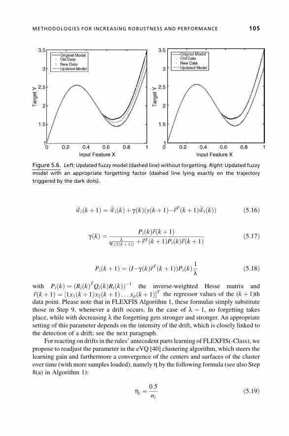
~wiðkþ 1Þ ¼ ~wiðkÞþ gðkÞðyðkþ 1Þ�~rTðkþ 1Þ~wiðkÞÞ ð5:16Þ

gðkÞ ¼ PiðkÞ~rðkþ 1Þl

Yið~xðkþ 1ÞÞ þ~rTðkþ 1ÞPiðkÞ~rðkþ 1Þ ð5:17Þ

Piðkþ 1Þ ¼ ðI�gðkÞ~rTðkþ 1ÞÞPiðkÞ 1l ð5:18Þ

with PiðkÞ ¼ ðRiðkÞTQiðkÞRiðkÞÞ�1 the inverse-weighted Hesse matrix and

~rðkþ 1Þ ¼ ½1x1ðkþ 1Þx2ðkþ 1Þ . . . xpðkþ 1Þ�T the regressor values of the (kþ 1)th

data point. Please note that in FLEXFIS Algorithm 1, these formulas simply substitute

those in Step 9, whenever a drift occurs. In the case of l ¼ 1, no forgetting takes

place, while with decreasing l the forgetting gets stronger and stronger. An appropriate

setting of this parameter depends on the intensity of the drift, which is closely linked to

the detection of a drift; see the next paragraph.

For reacting on drifts in the rules’ antecedent parts learning of FLEXFIS(-Class), we

propose to readjust the parameter in the eVQ [40] clustering algorithm, which steers the

learning gain and furthermore a convergence of the centers and surfaces of the cluster

over time (with more samples loaded), namely h by the following formula (see also Step

8(a) in Algorithm 1):

hi ¼0:5

nið5:19Þ

Figure 5.6. Left:Updated fuzzymodel (dashed line) without forgetting. Right:Updated fuzzy

model with an appropriate forgetting factor (dashed line lying exactly on the trajectory

triggered by the dark dots).


From formula (5.19) it can be realized that the learning gain decreaseswith the number of

samples forming the ith rule (ni), which is a favorable characteristic in order to converge

to optimality in the least-squares sense (section 5.2). If a drift occurs in a data stream, this

favorable characteristic is not favorable any longer, as then centers and widths of the

cluster(s) should change to the new data distribution. Hence, we propose a successive

increase of the learning gain with more samples loaded, whenever a drift starts (here,

assuming this for the ith cluster):

hi ¼0:5

ni�fac*ni;drift ð5:20Þ

where ni;drift denotes the number of data samples forming cluster i since the start of the

drift. The factor fac in the denominator depends on ni and on the speed of the drift from

one distribution to the other: Whenever ni is high, fac should be high as well in order to

gain a significant increase, especially at the beginning of the drift; on the other hand,

when ni is low, fac can be kept low, as the already-available cluster is not really distinct

and can be easily formed according to the new data distribution. Whenever the speed is

high, fac should also be high, as a fast adaptation to the new situation is required. In

Figure 5.7 three parameter curves showing the development of hi are visualized when

using three different values of fac, assuming that a drift starts at ni ¼ 600 and ends at

ni ¼ 700.

Figure 5.7. Increasing learninggainhduringadrift phase (left-hand side), decreasing learning

gain h when back into normal mode (right-hand side), when applying fac ¼ 1 (solid line), 2

(dashed line), and 3 (dashed dotted line).


In Section 5.5, we will highlight how a gradual forgetting of consequent resp.

antecedent parameters of the rules improves the predictive accuracies of regression

models and classifiers.

5.4.3.2 Drift Detection. The remaining central question is how to detect a drift

automatically from the data, as only in very rare cases will an external operator give

feedback on this issue from outside to the evolving modeling process. The detection is

necessary, because the more data, fully and equally weighted, is used in the learning

process, the better the accuracies of the models usually become, if no concept drift has

occurred since the data arrived. In this sense, a permanent gradual forgetting during the

whole online modeling procedure would asymptotically create worse models, when no

drift occurs. On the other hand, when a drift occurs, the distribution of the older data

differs from the current distribution, so that the older data may be misleading and hence

need to be outdated. One possibility for doing drift detection in online data streams when

applying evolving rule-based models is by exploiting the “rule age” concept introduced

in [2]. The rule age tracks how a rule becomes less important and has been used less; that

is, it will get “older” quicker than the average rate of ageing. In this sense, the derivatives

of the rule age curves can be inspected and a detection alarm triggered whenever a

significant knee in the smoothed curve can be observed (i.e., by a high second derivative).

In this case, a rule is suddenly ageingmuch faster than before (i.e., a change in the formof

a drift or shift in the underlying data distribution is quite likely).

5.4.4 Toward Safer Extrapolation Behavior

When doing adaptation of premise parts in fuzzymodelswith the usage of fuzzy sets with

infinite support (especially with themost commonGaussian sets), it usually happens that

not all fuzzy sets possess the samewidth. This is due to the nature of online data streams,

where local areas (which are projected onto the axes to form the fuzzy sets) reflect

different system behaviors with different ranges. This can lead to undesirable extrap-

olation effects, when the outermost set is not the broadest one, as a kind of reactivation of

an inner membership function in the extrapolation region is caused (see Figure 5.8).

Figure 5.8. A fuzzy partitionwhere inner sets are broader than outer ones. Especially compare

the two rightmost sets ! reactivation of the inner set in the extrapolation region.


Especially compare the two rightmost fuzzy sets; the extrapolation region is based on the

range of the input variable in the data set (from 0 to 1.03).

Inner sets can be reactivated, which is a precarious thing, as an outermost set

usually stands for the most confidential information in the case of extrapolation as it is

the nearest one.

In principle, one may focus on a learning procedure with constraints on the

clustering process in order to ensure the same widths for all clusters and consequently

fuzzy sets; however, thismay cause a severe drop in predictive performance in the normal

range as the model may no longer correctly represent the actual data characteristics.

Hence, we pursue another possibility for overcoming this drawback, which is simply

keeping all inner fuzzy sets as they are andmodifying the outermost fuzzy sets by letting

them be constant at the membership degree 1 for the second half of their Gaussian

membership functions, causing a zero-order extrapolation behavior over the complete

range of the variables [49]. Another possibility (which prevents the definition of a

twofold membership function) is to transform each outermost Gaussian fuzzy set to a

sigmoid function defined by:

mijðxjÞ ¼1

1þ eð�aijðxj�bijÞÞð5:21Þ

based on the following two properties (leading to two equations in a and b):

1. The position of inflection point of the Gaussian fuzzy set is equal to those of the

sigmoid function.

2. At the center position of theGaussian set the value of the sigmoid function is 0.99

(as 1 is not possible).

The solution gives

aðrightÞj ¼ � ln 0:01

sðrightÞjbðrightÞj ¼ cðrightÞj�sðrightÞj

ð5:22Þ

for the rightmost fuzzy set and

aðleftÞj ¼ ln 0:01

sðleftÞjbðleftÞj ¼ cðleftÞj þsðleftÞj

ð5:23Þ

for the leftmost fuzzy set, substituting aij and bij in (5.21). Figure 5.9 demonstrates the

impact of this transformation figure based on a simple two-dimensional example, when

trying to regress 10�4sinð0:001x2Þx3þ e2 with e2 a normally distributed random noise

with s ¼ 5 on 700 samples lying in the range of 0 to 80; in all images the samplewise

mean-squared error is plotted, which is obtained on 100 samples lying in the extrap-

olation range of 81 to 100 (so, 5 samples between eachwhole-number pair) andwhich are


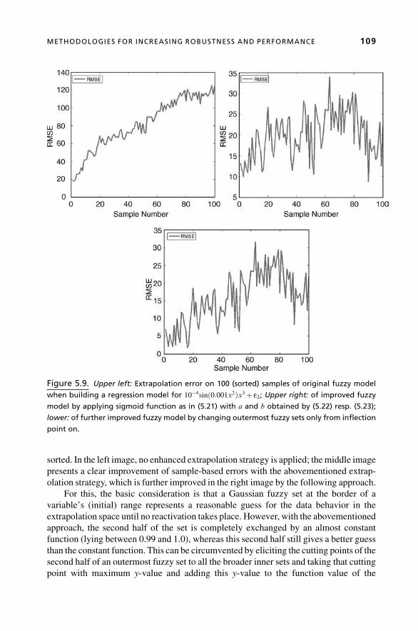
sorted. In the left image, no enhanced extrapolation strategy is applied; themiddle image

presents a clear improvement of sample-based errors with the abovementioned extrap-

olation strategy, which is further improved in the right image by the following approach.

For this, the basic consideration is that a Gaussian fuzzy set at the border of a

variable’s (initial) range represents a reasonable guess for the data behavior in the

extrapolation space until no reactivation takes place. However, with the abovementioned

approach, the second half of the set is completely exchanged by an almost constant

function (lying between 0.99 and 1.0), whereas this second half still gives a better guess

than the constant function. This can be circumvented by eliciting the cutting points of the

second half of an outermost fuzzy set to all the broader inner sets and taking that cutting

point with maximum y-value and adding this y-value to the function value of the

Figure 5.9. Upper left: Extrapolation error on 100 (sorted) samples of original fuzzy model

when building a regression model for 10�4sinð0:001x2Þx3þ e2; Upper right: of improved fuzzy

model by applying sigmoid function as in (5.21) with a and b obtained by (5.22) resp. (5.23);

lower: of further improved fuzzy model by changing outermost fuzzy sets only from inflection

point on.


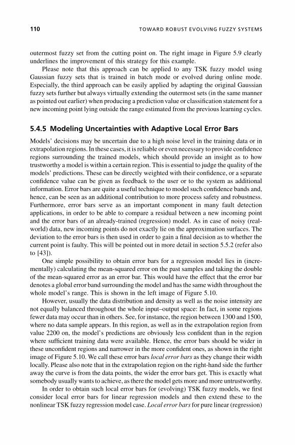
outermost fuzzy set from the cutting point on. The right image in Figure 5.9 clearly

underlines the improvement of this strategy for this example.

Please note that this approach can be applied to any TSK fuzzy model using

Gaussian fuzzy sets that is trained in batch mode or evolved during online mode.

Especially, the third approach can be easily applied by adapting the original Gaussian

fuzzy sets further but always virtually extending the outermost sets (in the same manner

as pointed out earlier) when producing a prediction value or classification statement for a

new incoming point lying outside the range estimated from the previous learning cycles.

5.4.5 Modeling Uncertainties with Adaptive Local Error Bars

Models’ decisions may be uncertain due to a high noise level in the training data or in

extrapolation regions. In these cases, it is reliable or evennecessary to provide confidence

regions surrounding the trained models, which should provide an insight as to how

trustworthy amodel is within a certain region. This is essential to judge the quality of the

models’ predictions. These can be directly weighted with their confidence, or a separate

confidence value can be given as feedback to the user or to the system as additional

information. Error bars are quite a useful technique to model such confidence bands and,

hence, can be seen as an additional contribution to more process safety and robustness.

Furthermore, error bars serve as an important component in many fault detection

applications, in order to be able to compare a residual between a new incoming point

and the error bars of an already-trained (regression) model. As in case of noisy (real-

world) data, new incoming points do not exactly lie on the approximation surfaces. The

deviation to the error bars is then used in order to gain a final decision as to whether the

current point is faulty. This will be pointed out in more detail in section 5.5.2 (refer also

to [43]).

One simple possibility to obtain error bars for a regression model lies in (incre-

mentally) calculating the mean-squared error on the past samples and taking the double

of the mean-squared error as an error bar. This would have the effect that the error bar

denotes a global error band surrounding themodel and has the samewidth throughout the

whole model’s range. This is shown in the left image of Figure 5.10.

However, usually the data distribution and density as well as the noise intensity are

not equally balanced throughout the whole input–output space: In fact, in some regions

fewer data may occur than in others. See, for instance, the region between 1300 and 1500,

where no data sample appears. In this region, as well as in the extrapolation region from

value 2200 on, the model’s predictions are obviously less confident than in the region

where sufficient training data were available. Hence, the error bars should be wider in

these unconfident regions and narrower in the more confident ones, as shown in the right

image of Figure 5.10. We call these error bars local error bars as they change their width

locally. Please also note that in the extrapolation region on the right-hand side the further

away the curve is from the data points, the wider the error bars get. This is exactly what

somebody usuallywants to achieve, as there themodel getsmore andmore untrustworthy.

In order to obtain such local error bars for (evolving) TSK fuzzy models, we first

consider local error bars for linear regression models and then extend these to the

nonlinear TSK fuzzy regressionmodel case. Local error bars for pure linear (regression)


models

f ð~xÞ ¼ y ¼Xdegi¼1

wi*regið~xÞ ð5:24Þ

with regi the ith regressor term applied to input variables x1; :::;xp, whose linear

parameters w were estimated by solving the least-squares optimization function, can

be calculated through the following formula [14]:

y�ffiffiffiffiffiffiffiffiffiffiffiffiffiffiffiffiffiffiffiffiffiffiffiffiffiffidiagðcovfygÞ

pð5:25Þ

where y is the estimated output value from (5.24) and

covfyg ¼ Xactcovfs2ðXTXÞ�1gXTact ð5:26Þ

The noise variance s can be estimated by

s2 ¼2XNj¼1ðyðjÞ�yðjÞÞ2

N�deg ð5:27Þ

where N is the number of data points, deg is the number of degrees of freedom (the

number of parameters in the linear case), X is the regression matrix, Xact is the matrix

containing the actual data points for which the error bars should be calculated, and yðjÞare themeasured values of the target. Note that the smaller the number of data points and/

or the higher the noise in the data, the higher the noise variance gets.

Figure 5.10. Left: Global model error band (light lines surrounding the darker line¼ fuzzy

model).Right: Local error barsgivingmoreprecise local informationabout the confidenceof the

model (taking into account holes in the data and extrapolation regions).


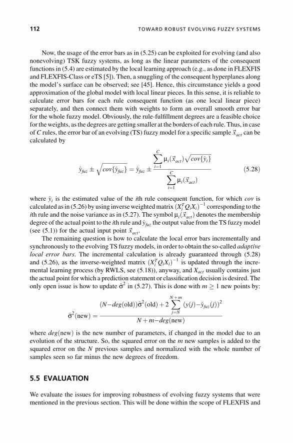
Now, the usage of the error bars as in (5.25) can be exploited for evolving (and also

nonevolving) TSK fuzzy systems, as long as the linear parameters of the consequent

functions in (5.4) are estimated by the local learning approach (e.g., as done in FLEXFIS

and FLEXFIS-Class or eTS [5]). Then, a snuggling of the consequent hyperplanes along

the model’s surface can be observed; see [45]. Hence, this circumstance yields a good

approximation of the global model with local linear pieces. In this sense, it is reliable to

calculate error bars for each rule consequent function (as one local linear piece)

separately, and then connect them with weights to form an overall smooth error bar

for the whole fuzzy model. Obviously, the rule-fulfillment degrees are a feasible choice

for theweights, as the degrees are getting smaller at the borders of each rule. Thus, in case

ofC rules, the error bar of an evolving (TS) fuzzy model for a specific sample~xact can becalculated by

yfuz �ffiffiffiffiffiffiffiffiffiffiffiffiffiffiffiffiffifficovfyfuzg

q¼ yfuz �

XCi¼1

mið~xactÞffiffiffiffiffiffiffiffiffiffiffiffiffiffifficovfyig

pXCi¼1

mið~xactÞð5:28Þ

where yi is the estimated value of the ith rule consequent function, for which cov is

calculated as in (5.26) by using inverseweightedmatrix ðXTi QiXiÞ�1 corresponding to the

ith rule and the noise variance as in (5.27). The symbol mið~xactÞ denotes the membership

degree of the actual point to the ith rule and yfuz the output value from the TS fuzzymodel

(see (5.1)) for the actual input point ~xact.The remaining question is how to calculate the local error bars incrementally and

synchronously to the evolving TS fuzzymodels, in order to obtain the so-called adaptive

local error bars. The incremental calculation is already guaranteed through (5.28)

and (5.26), as the inverse-weighted matrix ðXTi QiXiÞ�1 is updated through the incre-

mental learning process (by RWLS, see (5.18)), anyway, and Xact usually contains just

the actual point for which a prediction statement or classification decision is desired. The

only open issue is how to update s2in (5.27). This is done with m � 1 new points by:

s2ðnewÞ ¼ðN�degðoldÞÞs2ðoldÞþ 2

XNþm

j¼NðyðjÞ�yfuzðjÞÞ2

Nþm�degðnewÞwhere degðnewÞ is the new number of parameters, if changed in the model due to an

evolution of the structure. So, the squared error on the m new samples is added to the

squared error on the N previous samples and normalized with the whole number of

samples seen so far minus the new degrees of freedom.

5.5 EVALUATION

We evaluate the issues for improving robustness of evolving fuzzy systems that were

mentioned in the previous section. This will be done within the scope of FLEXFIS and


FLEXFIS-ClassMM approaches.We exploit three different online data sets, that is, data

sets that were collected within an online production process and stored onto hard disc

exactly in the same order as they appeared during the online process. In this sense, we

could simulate online mode in an offline program by simply taking sample by sample

from the data collection (row per row from a data matrix) and sending these for

incremental learning to FLEXFIS and FLEXFIS-Class respectively. We examine three

application cases:

1. Building an online prediction model for the resistance value at rolling mills

(applying FLEXFIS).

2. Online fault detection at engine test benches (applying FLEXFIS): This includes

a complete online system identification step of several high-dimensional regres-

sion models, representing different system dependencies, and together with their

adaptive local error bars serving as reference models for detecting faults in the

system.

3. Online image classification (applying FLEXFIS-Class MM) for supervising CD

imprint production processes and eggs.

In all cases, we are dealing with high-dimensional data (ranging from 32 to 74 input

variables/features, so regularization is essential) and in some caseswith smaller or bigger

drifts in the data streams. In the case of the engine test bench data, there are several

steady-state data included (so overcoming the unlearning effect is necessary), always

appearing after a significant change in rotation speed and torquewasmade in order to find

the balance for the new operating condition.

Note: For an empirical comparison of (conventional) FLEXFIS with other evolving

fuzzy systems techniques such as eTS, exTS, DENFIS, MRAN, RANEKF, SAFIS,

SOFNN, and GDFNN on both a high-dimensional approximation and a dynamic

identification problem, refer to [41]. For a detailed analytical and empirical comparison

with eTS, refer to [6]. For an empirical comparison of (conventional) FLEXFIS-Class

MM with eClass, refer to [3].

5.5.1 Online Prediction at Rolling Mills

The task was to identify a prediction model for the resistance value of a steel plate at a

rolling mill. This should be done in a first step with some offline (pre-collected)

measurement data in order to obtain a feeling about the achieved quality of the fuzzy

model and then to refine the predictionmodel with newly recorded online data. The latter

step was possible as first a prediction for the resistance is given, influencing the whole

process at the rolling mill, whereas a few seconds later (after the steel plate is passed) the

real value for the resistance is measured, which can then be incorporated into the model

adaptation process. In this sense, it is not the predicted (and maybe wrong) value that is

taken for further adaptation, but the correct measured value; hence, this can be seen as a

potential procedure for improving the models. The initial situation was as follows: An

analytical model was already available where some parameters were estimated through

EVALUATION 113

linear regression and should be improved by the fuzzy model component FLEXFIS,

whichwas applied purely based onmeasurement data. The analyticalmodel is physically

motivated by material laws that go back to Spittel and Hensel [26]; in modified form, the

resistance value can be estimated by an exponential function of the temperature, speed,

and thickness of the steel plate. Approximately 6000 training data points and approx-

imately 6000 online data points including 13 system variables (12 inputs, 1 output), such

as thickness of the steel plate before and after the rollingmill, average temperature, grain

size, and others, were collected during online production. Time delays up to 10 were

added for each input variable, leading to 121 input channels. The maximal delay was set

to 10, as from the experience of the operators it is known that the resistance value is

affected by influence values recorded maximally 8 to 10 passes ago (where one pass

delivers one measurement). A 10-fold cross-validation procedure [56] with the training

data was conducted for different parameter settings, varying the number of rules in the

fuzzy model and varying the input dimension from 1 to 20, whereas the most important

inputs were selected using amodified version of forward selection [20]. It turned out that

the maximal delay in any of the selected input variables was 8. The best-performing

fuzzy models obtained from the cross-validation step (Algorithm 1, Steps 1 and 2) were

compared on the independent online data with the analytical model in terms of mean

absolute error, the maximal errors from the upper and the lower side (estimated value too

high or too low), and the number of values as estimated 20 units too low than the

measured one (it was important to keep this error very low). Based on the best-

performing parameter setting, the fuzzy model was further adapted and evolved with

the online data, where for each sample a prediction was first given and then adapted with

the measured value. This was carried out with FLEXFIS (Algorithm 1, from Step 3 on).

The results are demonstrated in Table 5.1. The rows represent the different methods

applied, whereas the row “Static fuzzymodels” denotes the fuzzymodels obtained in the

offline CV step and not further updated with the separate online data set (so kept fixed

during the whole online prediction process), as opposed to the row “Evolving fuzzy

models,” where the fuzzy models are further evolved with Algorithm 1 from Step 3 on.

The columns represent the different validation measures. From this table it can be

realized that the results could be significantly improvedwhen using adaptation/evolution

of the models based on new measurements in parallel to the predictions, instead of

keeping them static. It is also remarkable that the static fuzzy models could outperform

the analytical model in offline mode.

T A B L E 5.1. Comparison of Evolving Fuzzy Prediction Models Obtained by FLEXFIS with anAnalytical and a Static Fuzzy Model for the Resistance Value at Rolling Mills

Method MAE

Max MAE Too High/Max

MAE Too Low/# MAEs> 20

Analytical 7.84 63.47 /87.37 /259

Static fuzzy models 5.41 38.05 /78.88 /159

Evolving fuzzy models 4.66 37.34 /75.43 /97

Evolving fuzzy models with grad. f. 4.34 31.99 /74.56 /68

Evolving fuzzy models no reg. 9.88 85.23 /151.21 /501


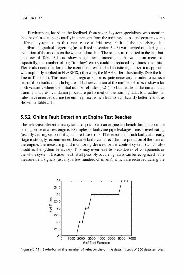
Furthermore, based on the feedback from several system specialists, who mention

that the online data set is totally independent from the training data set and contains some

different system states that may cause a drift resp. shift of the underlying data

distribution, gradual forgetting (as outlined in section 5.4.3) was carried out during the

evolution of the models on thewhole online data. The results are reported in the last-but-

one row of Table 5.1 and show a significant increase in the validation measures;

especially, the number of big “too low” errors could be reduced by almost one-third.

Please also note that for all the mentioned results the heuristic regularization approach

was implicitly applied in FLEXFIS; otherwise, theMAE suffers drastically. (See the last

line in Table 5.1). This means that regularization is quite necessary in order to achieve

reasonable results at all. In Figure 5.11, the evolution of the number of rules is shown for

both variants, where the initial number of rules (5.21) is obtained from the initial batch

training and cross-validation procedure performed on the training data; four additional

rules have emerged during the online phase, which lead to significantly better results, as

shown in Table 5.1.

5.5.2 Online Fault Detection at Engine Test Benches

The taskwas to detect asmany faults as possible at an engine test bench during the online

testing phase of a new engine. Examples of faults are pipe leakages, sensor overheating

(usually causing sensor drifts), or interface errors. The detection of such faults at an early

stage is strongly recommended, because faults can affect the interpretation of the state of

the engine, the measuring and monitoring devices, or the control system (which also

modifies the system behavior). This may even lead to breakdowns of components or

thewhole system. It is assumed that all possibly occurring faults can be recognized in the

measurement signals (usually, a few hundred channels), which are recorded during the

Figure 5.11. Evolution of the number of rules on the online data in steps of 300 data samples.

EVALUATION 115

test phase of an engine, and furthermore that most of the faults appear quite instan-

taneously. These include measurements of physical variables, such as pressures and

temperatures measured from sensors at different positions in the whole test bench cycle

(e.g., pressure of the oil is one important factor) and also all kind of emissions (NOX, CO2

etc.) whose values should be quite low in order to be in line with the legally allowed

boundary. Faults in the system may spoil these values and mislead the conclusion of an

engine under test and evaluation.

Our approach is now to identify high-dimensional relationships and dependencies

within the system, serving as (fault-free) reference models, which can be used to

calculate the deviation of new samples to these models (! residuals). As this

identification should be done fully automatically and without prior knowledge within

online operating mode in real time, it requires an incremental and evolving learning

mechanism for model building. In order not to be restricted to simple linear dependen-

cies, we exploit fuzzymodelswith highly nonlinear characteristics (and that are also able

to model linear dependencies). The noise is usually quite high at such engine test

benches, such that the integration of error bands surrounding the models into the fault

detection process is necessary.

In the case of global error bands, we exploit the whole model error (including bias

and variance error [24]), and the fault condition becomes (for m identified models,

see [43]):

9m :f fuz;k;m�xk;m�exmmodel�errorm

> thr _ f fuz;k;m�xk;mþ exmmodel�errorm

< �thr ð5:29Þ

with xk;m the actual (the kth) measured value of the target variable in the mth model

and f fuz;k;m the estimated output value from the mth first-order TSK fuzzy model as

defined in (5.1), and exm the inaccuracy in the target variables (recall: xm is the output

variable in themth model). In this sense, each fuzzymodel is checked with (5.29), and, if

this condition is fulfilled for at least one fuzzy model, the actual measurement (the kth)

is classified as faulty, otherwise as nonfaulty. This is quite intuitive, as faults usually

appear independently in one or more different measurement channels; hence, one

affected measurement channel is sufficient in order to trigger a fault alarm. Note

that thr is a threshold, usually set to a value of 2 for taking two times the model error

as error band.

As pointed out in section 5.4.5, local error bars achieve a good representation of the

data distribution in various local regions. In this sense, we extended the condition

in (5.29) to

9m :yfuz;k;m�xk;m�exmffiffiffiffiffiffiffiffiffiffiffiffiffiffiffiffiffiffiffiffiffiffiffiffiffi

covfyfuz;k;mgq > thr _ yfuz;k;m�xk;mþ exmffiffiffiffiffiffiffiffiffiffiffiffiffiffiffiffiffiffiffiffiffiffiffiffiffi

covfyfuz;k;mgq < �thr ð5:30Þ

including the local error bars (as in (5.28)) in the denominator of both conditions. In order

to overcome a hard-coded (offline) threshold thr and to achieve an adaptive online

thresholding concept, we analyzed the normalized residuals (according to the fault


condition)

resi¼1;:::;k�1;m ¼minðjyfuz;i;m�xi;m�exm j; jyfuz;i;m�xi;mþ exm jÞffiffiffiffiffiffiffiffiffiffiffiffiffiffiffiffiffiffiffiffiffiffiffiffi

covfyfuz;i;mgq ð5:31Þ

by univariate adaptive statistical methods exploiting a locally sliding regression model

for tracking the local trend of the residual signals adaptively over time. If anomalies in

these signals are observed (e.g., untypical peaks in case of outliertype faults or unusual

transients in case of drift-type faults), a fault alarm is triggered. In this sense, the fault

detection approach flexibly adapts to the current residual signal and does not imply one

unique threshold, which usually has totally different optimal values for different data sets

(engines to be tested). If the fault alarm is not confirmed as correct, the measurement can

be assumed to be fault-free and is taken into account for the further evolution of the fuzzy

models. On the other hand, if the fault alarm is confirmed as correct, the corresponding

residual resk is not sent into the parameter update of the local trend model and the

measurement is not taken into account for the evolution of the fuzzy models.

The evaluation test is performed onmeasurement data recorded from a BMWdiesel

engine. Eight different types of possibly occurring faults were simulated at an engine test

bench by switching off some components or reproducing leaks in pipes, and so on. In

sum, 7180 data pointswere recorded for 74 differentmeasurement channels. It turned out

that 56 measurement channels could be reasonably approximated with maximally five

others (reasonably approximatedmeans having amodel quality of greater than 0.8 where

1 would denote a perfect model), leading to m ¼ 1; . . . ; 56 evolving first-order TSK

fuzzy models, based on which the fault detection strategy mentioned earlier (i.e.,

incremental analysis of the residuals) is carried out online and samplewise. The results

are reported in Table 5.2, where basic fault detection with global error bands is compared

with improved fault detection logic, exploiting adaptive local error bars.

This comparison includes the detection rates on measurement basis (third column);

all measurements affected by faults are counted (in sum 80) as well as on the fault basis

(fourth column), that is, all different kinds of faults are counted (in sum eight). Column 2

represents the averagemodel quality over all 56 (reasonable)models (as quality measure

for the online identification part), which is measured in terms of the r-squared-adjusted

T A B L E 5.2. Comparison of Fault Detection Approaches on Real-Occurring Faults at anEngine Test Bench with the Usage of 56 Evolving Fuzzy Models Generated by FLEXFIS

Method

Average Model

Quality

Detection

Rate A

Detection

Rate B

Basic 0.958 71.59% 6 out of 8

Improved 0.958 87.50% 7 out of 8

Basic without overcoming

unlearning

0.913 64.23% 5 out of 8

Improved without overcoming

unlearning

0.913 72.83% 6 out of 8

EVALUATION 117

measure [23]:

R2adjusted ¼ 1�ðN�1Þð1�R

2ÞN�deg ð5:32Þ

where deg denotes the degrees of freedom (number of rules times the number of inputs)

and N the number of data points used for model training and R2defined by

R2 ¼ ssreg

ssregþ ssresð5:33Þ

where

ssreg ¼XNk¼1ðyðkÞ��yðkÞÞ2 ssres ¼

XNk¼1ðyðkÞ�yðkÞÞ2 ð5:34Þ

and �y the mean value of output target channel y. This measure is obviously normalized to

the unit interval and is nearer to 1 the smaller ssres is. Furthermore, it punishes more

complex models as integrating the degrees of freedom in the denominator.

Moreover, improved fault detection using local error bars can significantly outper-

form the basic one, as two faults more could be detected with the improved approach,

where one of these two was a major one and hence mandatory to be detected. Note that

rows 2 and 3 represent the results obtainedwhen integrating the approach for overcoming

the unlearning effect as outlined in section 5.4.2, that is, only to update the significantly

firing rules in Step 9 of FLEXFIS Algorithm 1. This is necessary as the online recorded

(dynamic) measurement data contain quite a lot of steady-state samples, that is, samples

showing an almost constant behavior in a lot of measurement channels over time (for

balancing out a new operating condition to get a valid and robust stationary data sample).

Rows 4 and 5 show the results suffering quite a bit when the approach for overcoming the

unlearning effect is omitted. The threshold here was set to 0.1, which gave best results

over various others (varied between 0 and 0.8 in steps of 0.05). A complete sensitivity

analysis of this threshold versus the change in fault detection rate achieved when using

adaptive local error bars is shown in Figure 5.12.

It can be seen that varying the threshold between 0.05 and 0.2 does not affect the fault

detection rate significantly. The average complexity measured in terms of the number of

rules of the finally evolved fuzzy models is 12.2 with a range of between 10 and 22 rules.

5.5.3 Online Image Classification Framework

An application example is given that includes an automatically self-reconfigurable and

adaptive image classification, which is shown in Figure 5.13.

The framework is able to cope with online operation modes and has a specific

component integrated for evolving classifiers based on operator feedback during online

production cycles. This human–machine interaction component is highlighted with an

ellipsoid in Figure 5.13 and serves as an essential part for improving initially offline-


trained classifiers further with new incoming images in order to extend classifiers to new

operating conditions (e.g., new types of images) and, hence, to prevent extrapolation and

a low classification performance. Please note that initially offline-trained classifiers

(from prelabeled training data) are mandatory as giving the experts a first hint as to

whether the classification task can be reasonably trained at all up to a certain (predefined)

level of accuracy, yielding a prediction about the success or failure of the classifier [55].

After preprocessing the images by comparing themwith amaster to obtain deviation

images, where each pixel represents a potential candidate for indicating a fault, regions

of interest are automatically recognized and for each region a large set of object features

are extracted. Examples of object features describing the characteristics of a region of

interest are ratio of the principal axis to the secondary axis of a circumscribing ellipse

(roundness), perimeter, area, compactness, and statistical values such as curtosis, skew,

or different quantiles out of the corresponding gray-level histograms. These are

completed with a set of aggregated features characterizing images as a whole, and so,

characterizing all pixels and objects joined together. Examples of aggregated features are

the number of objects, the maximal density of objects, or the average brightness in an

image. Classification of the images is done into good or bad ones, indicating fault-free or

Figure 5.12. Sensitivity analysis for the threshold in FLEXFIS for overcoming the unlearning

effect.

Figure 5.13. Online classification framework for classifying images into good and bad.

EVALUATION 119

faulty situations at the system. Depending on the level of detail the user gives to the

system (i.e., labeling only whole images or also single objects), the classification of

whole images is done either based on aggregated features plus unsupervised object

information (produced by aggregation operators or by clustering approaches on the

object features) or by aggregated features plus supervised object information obtained as

output from an object-level classifier. (For details see [54].) Here, we report results on the

former approach, including 74 features (57 object features plus 17 aggregated features)

and based on two different data sets:

1. Online collected CD-imprint data containing 1534 samples that were labeled by

four different operators with different experiences (so, we obtained four different

classifiers with different accuracies): The task was to distinguish between real

faults onCD imprints such asweak colors,wrong palettes, and so on, and pseudo-

errors such as shifts of discs in the tray.

2. Online collected egg data containing 4238 samples labeled by just one operator:

The task was to discriminate between real faults on eggs, such as scratches or

yolks, and nonfaulty appearances on the eggs, such as different kinds of dirt.

In both cases, the online collected data were stored onto hard-disc in the same order as

they were recorded; so a valid simulation of the online mode is the case when sending

sample per sample into the evolution of the fuzzymodels and taking the label entries as a

simulation of online operator feedback.

Both data sets were split into a training data set (two-thirds of the data) and a test data

set (one-third of the data). The training datawas split into two halves, one taken for initial

offline training, the other for further evolution of the classifiers. The test data set is for the

purpose of evaluating the evolved classifiers on new unseen data. Table 5.3 shows the

performance of evolving classifiers obtained by FLEXFIS-Class MM (see Algorithm 2)

vs. static classifiers trained in initial offline mode with the first batch of data and not

further updated, based on the CD-imprint data. It can be seen that by doing an adaptation

during online mode the performance on new unseen samples significantly increases by

10 to 15% over all operators as well as for the egg data. Furthermore, the third row shows

us that, when retraining a batch decision-tree classifier on all training samples (the well-

known CARTalgorithm [10], which was the best-performing one on this data set among

T A B L E 5.3. Performance (Accuracy in%) of Evolving Online vs. Static (and Retrained) BatchClassifiers

Dataset Op. 1 Op. 2 Op. 3 Op. 4 Eggs

Fuzzy classifier static 68.63 85.29 85.68 78.24 76.08

Fuzzy classifier retrained 86.23 89.11 90.55 87.02 93.93

Evolving fuzzy classifier 84.12 88.06 89.92 86.90 93.6

Evolving fuzzy classifier every 5 84.05 88.01 89.44 85.99 93.11

Decision trees static 70.94 78.82 80.00 76.08 91.73

Decision trees retrained 82.74 90.59 90.39 88.24 96.6


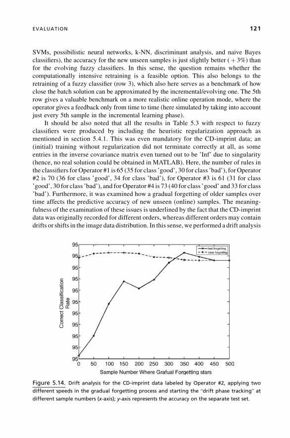
SVMs, possibilistic neural networks, k-NN, discriminant analysis, and naive Bayes

classifiers), the accuracy for the new unseen samples is just slightly better (þ 3%) than

for the evolving fuzzy classifiers. In this sense, the question remains whether the

computationally intensive retraining is a feasible option. This also belongs to the

retraining of a fuzzy classifier (row 3), which also here serves as a benchmark of how

close the batch solution can be approximated by the incremental/evolving one. The 5th

row gives a valuable benchmark on a more realistic online operation mode, where the

operator gives a feedback only from time to time (here simulated by taking into account

just every 5th sample in the incremental learning phase).

It should be also noted that all the results in Table 5.3 with respect to fuzzy

classifiers were produced by including the heuristic regularization approach as

mentioned in section 5.4.1. This was even mandatory for the CD-imprint data; an

(initial) training without regularization did not terminate correctly at all, as some

entries in the inverse covariance matrix even turned out to be ’Inf’ due to singularity

(hence, no real solution could be obtained in MATLAB). Here, the number of rules in

the classifiers for Operator #1 is 65 (35 for class ’good’, 30 for class ’bad’), for Operator

#2 is 70 (36 for class ’good’, 34 for class ’bad’), for Operator #3 is 61 (31 for class

’good’, 30 for class ’bad’), and for Operator #4 is 73 (40 for class ’good’ and 33 for class

’bad’). Furthermore, it was examined how a gradual forgetting of older samples over

time affects the predictive accuracy of new unseen (online) samples. The meaning-

fulness of the examination of these issues is underlined by the fact that the CD-imprint

data was originally recorded for different orders, whereas different orders may contain

drifts or shifts in the image data distribution. In this sense, we performed a drift analysis

Figure 5.14. Drift analysis for the CD-imprint data labeled by Operator #2, applying two

different speeds in the gradual forgetting process and starting the “drift phase tracking” at

different sample numbers (x-axis); y-axis represents the accuracy on the separate test set.

EVALUATION 121

with different starting points (beginning with gradual evolution at 0, 50, 100, 150, . . .,500 online samples), lasting over 50 samples in the drift phase and with two different

speeds for gradual forgetting. The results for Operator #2 are shown in Figure 5.14,

where the slow gradual forgetting is denoted by the dotted-dashed line and the fast

gradual forgetting by the solid line. The sample number in the second half of the

training set at which the drift is initialized is represented by the x-axis; the achieved

accuracies on separate test data when including the gradual forgetting on the rest of the

second half of the training data are represented by the y-axis. In fact, the accuracies for

Operator #2 can be boosted up by about 3% (to 91.39% maximum) when initiating a

drift phase at the correct sample number and taking the appropriate speed in the gradual

forgetting process. In our case, this means that a slow forgetting starting between 100

and 150 and a fast forgetting starting at 350 is beneficial, tracking two different types of

drifts. In fact, when combining these two, a classification rate of even over 92% can be

achieved, gaining another 1% accuracy.

Moreover, the class distribution of the CD-imprint data is quite unbalanced as only

around 20% of bad samples could be gathered from the production process. In this sense,

we applied the “timing of update” strategy mentioned at the end of section 5.4.2; that is,

we updated the fuzzy classifier only with samples from the ’good’ class in the case of a

disagreement of the classification decision and the true class label of the new sample.

This gave us another 1.4%more accuracy on the CD-imprint data, compared to the 92%

achieved with double drift tracking.

5.6 CONCLUSION

In this chapter we demonstrated several issues for obtaining more robustness, process

safety, and higher predictive accuracies when doing an evolution of fuzzy models based

on online data, and underlined the importance of these issues with graphical visualiza-

tions. All of these issues were implemented within the scope of the FLEXFIS and

FLEXFIS-Class approaches which borrow from eTS and eClass approaches, respec-

tively. The evaluation section shows quite promising results when applying some of these

issues for three different real-world applications, including online fault detection at

engine test benches, online image classification based on operator feedback, and online

prediction at rolling mills. Sometimes, some of these issues were even mandatory in

order to obtain any reasonable and robust prediction or classification feedbacks at all. In

most cases, several issues could guide the evolved fuzzymodels tomore predictive power

in terms of accuracy, especially in the case of steady-state data or a smoothly changing

behavior of the underlying data distribution in the form of a drift. Robustness in terms of

the performance of evolving fuzzy models coming close to the batch performance could

be also shown. The approaches for improving robustness are applicable for other

evolving fuzzy modeling methods as well, especially for those that exploit TSK

(neuro-)fuzzy-type architectures (all issues)—respectively, fuzzy sets with infinite

support (better extrapolation behavior, overcoming unlearning effect) and/or polynomial

consequent functions (adaptive local error bars, regularization, tracking drifts)—but are

not necessarily restricted to these. In this sense, these approaches can be seen as an


important step in the future in order to achieve much richer evolving fuzzy modeling

components in intelligent systems.

5.7 ACKNOWLEDGMENTS

This work was supported by the European Commission (Project Contract No.

STRP016429, acronym DynaVis) and by the the Upper Austrian Technology and

Research Promotion. This chapter reflects only the author’s view.

5.8 REFERENCES

1. J. Abonyi, Fuzzy Model Identification for Control. Boston: Birkh€auser, 2003.

2. P.Angelov,D. Filev, “Simpl_eTS:ASimplifiedMethod forLearningEvolvingTakagi-Sugeno

Fuzzy Models.” Proceedings of FUZZ-IEEE 2005, Reno, Nevada, 2005, pp. 1068–1073.

3. P. Angelov, X. Zhou, D. Filev, E. Lughofer, “Architectures for Evolving Fuzzy Rule-Based

Classifiers.” Proceedings of SMC 2007, Montreal, Canada, 2007, pp. 2050–2055.

4. P. Angelov, X. Zhou, F. Klawonn, “Evolving Fuzzy Rule-Based Classifiers.” 2007 IEEE

International Conference on Computational Intelligence Application for Signal and Image

Processing, Honolulu, Hawaii, 2007 pp. 220–225.

5. P.P. Angelov, D. Filev, “An Approach to Online Identification of Takagi-Sugeno Fuzzy

Models,” IEEE Trans. on Systems, Man and Cybernetics, Part B, 34 (1): 484–498, 2004.

6. P. P. Angelov, E. Lughofer, “Data-Driven Evolving Fuzzy Systems Using eTS and FLEXFIS:

Comparative Analysis,” International Journal of General Systems, 37 (1): 45–67, 2008.


8. J. C. Barros, A. L. Dexter, “An Evolving Fuzzy Model for Embedded Applications.” Second

Int. Symposium on Evolving Fuzzy Systems, Lake District, UK, 2006, pp. 36–41.

9. F. Bauer, “Some Considerations Concerning Regularization and Parameter Choice

Algorithms,” Inverse Problems, 23: 837–858, 2007.

10. L. Breiman, J. Friedman, C. J. Stone, R. A. Olshen,Classification and Regression Trees. Boca

Raton: Chapman and Hall, 1993.

11. G. A. Carpenter, S. Grossberg, “Adaptive Resonance Theory (art).” In TheHandbook of Brain

Theory and Neural Networks. (M. A. Arbib, ed.) Cambridge: MIT Press, 1995, pp. 79–82.

12. J. Casillas, O. Cordon, F. Herrera, L. Magdalena, Interpretability Issues in Fuzzy Modeling.

Berlin, Heidelberg: Springer-Verlag, 2003.

13. D.Donoho, I. Johnstone, “MinimaxEstimationviaWavelet Shrinkage,”Annual Statistics, 26:

879–921, 1998.

14. N. R. Draper, H. Smith, Applied Regression Analysis: Probability and Mathematical

Statistics. New York: John Wiley & Sons, 1981.

15. R. O. Duda, P. E. Hart, D. G. Stork, Pattern Classification, Second Edition. Southern Gate,

Chichester, West Sussex PO 19 8SQ, England: Wiley-Interscience, 2000.

16. H.W. Engl, M. Hanke, A. Neubauer,Regularization of Inverse Problems. Dordrecht: Kluwer,

1996.

REFERENCES 123

17. D. P. Filev, F. Tseng, “Novelty Detection BasedMachine Health Prognostics.” Proc. 2006 Int.

Symposium on Evolving Fuzzy Systems, Lake District, UK, 2006, pp. 193–199.

18. R. M. Gray, “Vector Quantization,” IEEE ASSP, pages 4–29, 1984.

19. C. W. Groetsch, The theory of Tikhonov regularization for Fredholm Equations of the First

Kind. Boston: Pitman, 1984.

20. W.Groißb€ock, E. Lughofer, E. P.Klement, “AComparison ofVariable SelectionMethodswith

the Main Focus on Orthogonalization.” In Soft Methodology and Random Information

Systems: Advances in Soft Computing. (M. Lop�ez-D�ıaz, M. A. Gil, P. Grzegorzewski, O.

Hryniewicz, J. Lawry, ed.) Berlin, Heidelberg, New York: Springer, 2004, pp. 479–486.

21. N. Sundararajan, H.-J. Rong, G.-B. Huang, P. Saratchandran, “Sequential Adaptive Fuzzy

Inference System (SAFIS) for Nonlinear System Identification and Prediction,” Fuzzy Sets

and Systems, 157 (9): 1260–1275, 2006.

22. P. C. Hansen, “The truncated svd as a Method for Regularization,” BIT, 27: 534–553, 1987.

23. F. E. Harrel. Regression Modeling Strategies. New York: Springer-Verlag New York, 2001.

24. T. Hastie, R. Tibshirani, J. Friedman, The Elements of Statistical Learning: Data Mining,

Inference and Prediction. New York, Berlin, Heidelberg: Springer-Verlag, 2001.

25. S.Haykin,Neural Networks: AComprehensive Foundation, 2nd Edition.Upper Saddle River,

NJ: Prentice Hall, 1999.

26. A. Hensel, T. Spittel, Kraft- und Arbeitsbedarf bildsamer Formgebungsverfahren. VEB

Deutscher Verlag f€ur Grundstoffindustrie, 1978.

27. G. B.Huang, P. Saratchandran, N. Sundararajan, “AnEfficient Sequential LearningAlgorithm

for Growing and Pruning RBF (GAP-RBF) Networks,” IEEE Transactions on Systems, Man

and Cybernetics, Part B (Cybernetics), 34 (6): 2284–2292, 2004.

28. R. Iserman, Fault Diagnosis Systems: An Introduction from Fault Detection to Fault

Tolerance. Berlin: Springer-Verlag, 2005.

29. H. Ishibushi, T. Nakashima, T. Murata, “Performance Evaluation of Fuzzy Classifier Systems

for Multidimensional Pattern Classification Problems,” IEEE Transactions on Systems, Man

and Cybernetics, Part B (Cybernetics), 29 (5): 601–618, 1999.

30. H. Ishibushi, Y. Nojima, “Analysis of Interpretability-Accuracy Tradeoff of Fuzzy Systems by

Multiobjective Fuzzy Genetics-Based Machine Learning,” Int. Journal of Approximate

Reasoning, 44 (1): 4–31, 2007.

31. T. A. Johansen, R. Babuska, “Multiobjective Identification of Takagi-Sugeno FuzzyModels,”

IEEE Transactions on Fuzzy Systems, 11 (6): 847–860, 2003.

32. N. Kasabov, Evolving Connectionist Systems: Methods and Applications in Bioinformatics,

Brain Study and Intelligent Machines. London: Springer-Verlag, 2002.

33. N. K. Kasabov, “Evolving Fuzzy Neural Networks for Supervised/Unsupervised Online

Knowledge-Based Learning,” IEEE Trans. on Systems, Men and Cybernetics, Part B

(Cybernetics), 31 (6): 902–918, 2001.

34. N. K. Kasabov, Q. Song, “DENFIS: Dynamic Evolving Neural-Fuzzy Inference System and Its

Application for Time-Series Prediction,” IEEETrans. onFuzzy Systems, 10 (2): 144–154, 2002.

35. C. C. Lee, “Fuzzy Logic in Control Systems: Fuzzy Logic Controller, Parts I and II,” IEEE

Trans. System, Man, Cybernetics, 20: 404–435, 1990.

36. G. Leng, T. M.. McGinnity, G. Prasad, “An Approach for On-line Extraction of Fuzzy Rules

Using a Self-Organising Fuzzy Neural Network,” Fuzzy Sets and Systems, 150 (2): 211–243,

2005.


37. O. V. Lepskij, “On a Problem of Adaptive Estimation in Gaussian White Noise,” Theory of

Probability and its Applications, 35 (3): 454–466, 1990.

38. E. Lima, F. Gomide, R. Ballini, “Participatory Evolving Fuzzy Modeling.” Second Int.

Symposium on Evolving Fuzzy Systems, Lake District, UK, 2006, pp. 36–41.

39. L. Ljung, System Identification: Theory for the User. Upper Saddle River, NJ: Prentice Hall

PTR, Prentice-Hall, 1999.

40. E. Lughofer, “Extensions of Vector Quantization for Incremental Clustering,” Pattern

Recognition, 41 (3): 995–1011, 2008.

41. E. Lughofer, “FLEXFIS: A Robust Incremental Learning Approach for Evolving TS Fuzzy

Models,” IEEE Trans. on Fuzzy Systems (Special Issue On Evolving Fuzzy Systems), 16 (4):

1–18, 2008.

42. E. Lughofer, P. Angelov, X. Zhou, “Evolving Single- andMulti-Model Fuzzy Classifiers with

FLEXFIS-Class.” Proceedings of FUZZ-IEEE 2007, London, UK, 2007 pp. 363–368.

43. E. Lughofer, C.Guardiola, “ApplyingEvolvingFuzzyModelswithAdaptive Local Error Bars

to On-line Fault Detection.” Proceedings of Genetic and Evolving Fuzzy Systems 2008,

Witten-Bommerholz, Germany, 2008, pp. 35–40.

44. E. Lughofer, C. Guardiola, “On-line Fault Detection with Data-Driven Evolving Fuzzy

Models,” Journal of Control and Intelligent Systems, 36 (2), 2008.

45. E. Lughofer, E. H€ullermeier, E. P. Klement, “Improving the Interpretability of Data-Driven

Evolving Fuzzy Systems.” Proceedings of EUSFLAT 2005, Barcelona, Spain, 2005, pp. 28–33.

46. J. G. Qiang Shen Marin-Blazquez, “From Approximative to Descriptive Fuzzy Classifiers,”

IEEE Transactions on Fuzzy Systems, 10 (4): 484–497, 2002.

47. V. A. Morozov, “On the Solution of Functional Equations by the Methdod of Regularization,”

Sov. Math. Dokl, 7: 414–417, 1965.

48. D.Nauck, R.Kruse, “ANeuro-FuzzyMethod to Learn FuzzyClassificationRules fromData,”

Fuzzy Sets and Systems, 89(3): 277–288, 1997.

49. A. Piegat, Fuzzy Modeling and Control. Heidelberg, New York: Physica Verlag, Springer-

Verlag, 2001.

50. F. Provost, “Machine Learning from Imbalanced Data Sets.” Proceedings of the AAAI

workshop, Menlo Park, CA, 2000, pp. 1–3.

51. S. J. Qin, W. Li, H. H. Yue, “Recursive PCA for Adaptive Process Monitoring,” Journal of

Process Control, 10: 471–486, 2000.

52. J. A. Roubos, M. Setnes, J. Abonyi, “Learning Fuzzy Classification Rules from Data,”

Information Sciences—Informatics and Computer Science: An International Journal, 150:

77–93, 2003.

53. D. Donoho, S. Chen, M. Saunders, “Atomic decomposition by basis pursuit,” SIAM Rev., 43

(1): 129–159, 2001.

54. D. Sannen,M. Nuttin, J. E. Smith,M. A. Tahir, E. Lughofer, C. Eitzinger, “An Interactive Self-

Adaptive On-line Image Classification Framework.” In, Proceedings of ICVS 2008, Vol. 5008

of LNCS ( A. Gasteratos, M. Vincze, J. K. Tsotsos, ed.) Santorini Island, Greece: Springer,

2008 pp. 173–180.

55. J. E. Smith,M.A. Tahir, “StopWastingTime:OnPredicting the Success or Failure of Learning

for Industrial Applications.” Proccedings of the 8th International Conference on Intelligent

Data Engineering and Automated Learning (IDEAL’08), Lecture Notes in Computer Science,

LNCS 4881. Birmingham, UK: Springer-Verlag, 2007, pp. 673–683.

REFERENCES 125

56. M. Stone, “Cross-Validatory Choice andAssessment of Statistical Predictions,” Journal of the

Royal Statistical Society, 36: 111–147, 1974.

57. A. N. Tikhonov, V. Y. Arsenin, Solutions of Ill-Posed Problems. Washington D.C.:Winston &

Sonst, 1977.

58. N. Tschichold-Guerman, “Generation and Improvement of FuzzyClassifierswith Incremental

Learning Using Fuzzy Rulenet.” Proceedings of the 1995 ACM Symposium on Applied

Computing, Nashville, Tennessee, 1995, ACM Press, New York.

59. A. Tsymbal, “The Problem of Concept Drift: Definitions and Related Work.” Technical

Report TCD-CS-2004-15, Department of Computer Science, Trinity College Dublin, Ireland,

2004.

60. G. C. van den Eijkel, J.C.A. van der Lubbe, E. Backer, “Fuzzy Incremental Learning of Expert

Rules for aKnowledge-BasedAnesthesiaMonitor.”Fourth EuropeanCongress on Intelligent

Techniques and Soft Computing Proceedings, EUFIT ’96, Verlag Mainz, 1996, pp.

2056–2060.

61. L. X.Wang, J. M.Mendel, “Fuzzy Basis Functions, Universal Approximation andOrthogonal

Least-Squares Learning,” IEEE Trans. Neural Networks, 3(5): 807–814, 1992.

62. G. Widmer, M. Kubat, “Learning in the Presence of Concept Drift and Hidden Contexts,”

Machine Learning, 23(1): 69–101, 1996.

63. S. Wu, M. J. Er, “Dynamic Fuzzy Neural Networks: A Novel Approach to Function

Approximation,” IEEE Trans. on Systems, Man and Cybernetics, Part B (Cybernetics),

30: 358–364, 2000.

64. S. Wu, M. J. Er, Y. Gao, “A Fast Approach for Automatic Generation of Fuzzy Rules by

Generalized Dynamic Fuzzy Neural Networks,” IEEE Trans. on Fuzzy Systems, 9(4):

578–594, 2001.

65. R. Yager, D. Filev, “Generation of Fuzzy Rules by Mountain Clustering.” Technical Report

MII-1318R, Machine Intelligence Institute, Iona College, New Rochelle, NY 10801, 1994.

66. R. R. Yager, “A Model of Participatory Learning,” IEEE Trans. on Systems, Man and

Cybernetics, 20: 1229–1234, 1990.

67. J. Yen, L. Wang, C. W. Gillespie, “Improving the Interpretability of TSK Fuzzy Models by

Combining Global Learning and Local Learning,” IEEE Trans. on Fuzzy Systems, 6(4):

530–537, 1998.


6

BUILDING INTERPRETABLESYSTEMS IN REAL TIMEJos�e V. Ramos, Carlos Pereira, Antonio Dourado

Abstract: Building interpretable learning machines from data, incrementally, with the

capability for a-posteriori knowledge extraction, is still a big challenge. It is difficult to

avoid some degree of redundancy and unnecessary complexity in the obtained models.

This work presents two alternative ways for building interpretable systems, using fuzzy

models or kernel machines. The goal is to control the complexity of the machine, either

the number of rules or the number of kernels, using incremental learning techniques and

merging of fuzzy sets. In the first case, online implementation of mechanisms for

merging membership functions and rule base simplification, toward evolving first-order

Takagi-Sugeno fuzzy systems (eTS), is proposed in this chapter in order to improve the

interpretability of the fuzzy models. As a comparative solution, kernel-based methods

may also contribute to the interpretability issue, particularly the incremental learning

algorithms. The interpretability is analyzed based on equivalence principles between

local model networks and Takagi-Sugeno fuzzy inference systems.

A considerable reduction of redundancy and complexity of the models is obtained,

increasing the model transparency and human interpretability. The learning technique

is developed for large spanned evolving first-order Takagi-Sugeno (eTS) fuzzy models.

The benchmark of the Box-Jenkins time-series prediction is used to evaluate the

techniques.


and Nikola Kasabov


6.1 INTRODUCTION

Every year, more than 1 exabyte (1018 bytes) of data is generatedworldwide, most of it in

digital form [1]. Data-driven methodologies for automatic generation of computational

models are probably one of the most important tools needed to be developed to properly

process and use that immense quantity of information [2]. In most applications (industry,

medicine, finance, business, etc.), these methodologies should be iterative, to process

the data as it is being reported in real time, and transparent, building a linguistic model

clearly interpretable by humans. eTS (evolving Takagi-Sugeno systems) is one of those

methodologies [3]. In the present work, the eTS developed by [4] is improved, increasing

the rule-span in state space, and used to build fuzzy systems from data. Traditionally,

the most important property of a fuzzy system has been its accuracy in representing the

real system (for simulation, prediction, decision making, etc.).

However, the obtained fuzzy systems frequently arewithout practical utility because

it is impossible to give some semantic meaning to the rules due to fuzzy sets

superposition, and rules that are sometimes redundant and sometimes contradictory,

frequently with high complexity. In [5] a comprehensive collection of papers present

several approaches for evolving the fuzzy systems to more interpretability (mainly

offline trained or expert-based ones). In recent years, interpretability has been considered

to be the key feature of fuzzy models [6, 7], continuing previous important works [8, 9],

and can be pursued by rule base simplification and reduction methods. There is actually

considerable activity concerning this challenging problem. Several perspectives are

being developed, for example, by fuzzy set merging using entropy measures [10],

by genetic optimization [11–13], by multiobjective evolutionary algorithms [14–16],

by manipulating the cost index [17, 18], or by Radial Basis Function Networks [19]. For

a more detailed review and treatment, see [22] or [23]. Most of the known methods have

been developed for batch processing for an already-existing rule base.

Kernel-based learning methods, such as Support Vector Machines (SVMs), Rele-

vance Vector Machines (RVMs), or Kernel PCA, have been studied extensively in the

machine-learning community, being among the best learning techniques for many

benchmark data sets and real-world applications [24]. The basic idea of these methods

is topreprocess thedata by somenonlinearmapping (using thekernel trick) and thenapply

a linear algorithm in a usually higher-dimensional feature space. Such large feature spaces

are handled with the simple computational cost of the kernel function. This approach

indicates an alternative point of view to the parameters learning of a fuzzy system,with the

membership functions being those examples that are critical to solving the given task. In

the traditional forms of automatic learning, the functions are simply regarded as clusters.

The objective of the present chapter is online learning, for developingmodels in real

time for classification problems and dynamic systems. Computational time is a critical

issue and simple, efficient techniques are searched for. A pruning technique is developed

and tested to reduce the degree of redundancy and unnecessary complexity arising in the

automated building of fuzzy rules. This improves the human semantic interpretability

and as a consequence the usefulness of the results, allowing the merging of compatible

fuzzy sets and possibly reduction of the number of rules and features. The fuzzy system is

based on an improved version of the eTS algorithm of [4], strengthening its capability to

128 BUILDING INTERPRETABLE SYSTEMS IN REAL TIME

spread rules over all the reachable state space. Pruning of the rules is based on fusion of

the antecedents fuzzy sets subject on a similarity threshold and rule elimination based

on similar antecedents. The advantage of similarity measures, principally the geometric

ones, is there simplicity from the computational point of view, which is explored in this

work.

This chapter is organized as follows. The eTS of [4] is briefly reviewed in section 6.2

and conditions are proposed to increase the span of the rules in the state space. In

section 6.3 the pruning technique and merging of fuzzy rules is developed. In section 6.4

the interpretability is analyzed based on equivalence principles between local model

networks and Takagi-Sugeno fuzzy inference systems. In addition, methods to improve

the interpretability of the support vector machine are briefly discussed. Finally,

section 6.5 presents the application to the benchmark problem of Box-Jenkins dynamic

time-series prediction. The chapter ends with some conclusions and perspectives.

6.2 IMPROVING eTS SPAN IN THE REACHABLE STATE SPACE

Online learning of eTS fuzzy models, which is based on Takagi-Sugeno rules, considers

their online identification to be subject to gradually evolving rules. The procedure in the

present work includes recursive subtractive fuzzy clustering, for determination of the

antecedent parameters, and recursive least-squares estimation, for determination of

the consequent parameters. Angelov and Filev [4] developed an interesting technique for

recursive clustering and rule creation that is the starting and fulcral point for the present

proposal. The procedure can be summarized as follows:

Step 1: Initialization of the rule base.

The rule base is initially empty. Rules are created around the centers of the

input–output clusters, in the subtractive clustering framework. Let xk and yk be

the input and output vectors at instant k, respectively.When the first input–output

data is coming, z1 ¼ ½x1; y1�, it is the single existing cluster in the input–output

space and at the same time its own center z*1. P1(z1�) is the energy potential of the

cluster center z*1 to be used for subtractive clustering. The cluster center z*1 is a

multidimensional point (the number of dimensions is equal to the number of

inputs plus the number of outputs) and each input is an antecedent of each fuzzy

rule. To obtain from it a fuzzy set for each antecedent, one needs to project the

cluster center into each input dimension, and this projection gives the center of

the fuzzy set of each antecedent.

So the rule base is initialized with the first data sample, as in (6.1):

k ¼ 1; R ¼ 1; x*1 ¼ xk; P1ðz*1Þ ¼ 1 ð6:1Þwhere k is the actual sampling point, R is the actual number of rules, z*1 is the first

cluster center; x*1 is the focal point of the antecedent of first rule, obtained by

projecting z*1 on the input dimensions.

In a mixed-batch–real-time learning approach, the rule base can be initialized

by existing expert knowledge or based on previous offline identification, defining

IMPROVING eTS SPAN IN THE REACHABLE STATE SPACE 129

an initial set zi� of cluster centers and of initial rules, Rini. In this case, we

have (6.2):

R ¼ Rini; P1ðz*i Þ ¼ 1; i ¼ 1; . . . ;Rini ð6:2Þ

Step 2: Reading the next data sample.

In an online set, each input is coming in fixed successive instants of time. At the

next time step, instant k, the new data sample zk ¼ ½xk; yk� is collected. This newdata sample changes all the field energy and as a consequence the potential

energy of every existing center; the new potentials must then be calculated.

Step 3: Recursive calculation of the potentials of each new data sample (for

subtractive clustering).

For online learning, the potentials must be computed recursively, leading to

the need of recursive formulas for potentials like the Cauchy function (A1) of the

appendix proposed by [4] and adopted in this work.

Step 4:Recursive update of the potentials of existing centers taking into account the

influence of the new data sample.

This is made according to the method developed by [4].

Step 5: Upgrade of the rule base structure: Modify a rule or create a new one.

This is the essential stage in eTS philosophy. The potential of the newdata sample

is compared to the updated potential of existing centers; then the important

decision whether to modify or create a new rule is taken. This is a very sensitive

task and different scenarios have been empirically investigated for rule base

upgrade and modification. An extensive work undertaken in [17, 18] for a broad

set of problems allowed a better understanding about the influence on the creation

and modification of the rules and proposed new conditions described in the

following, improving the algorithm of [4].

6.2.1 Rule Base Upgrade: Improve Span over State Space

Two situations may arise:

1. The new data point spans over new regions of state-space, where previously no

point has been reached. This point has a very lowpotential because it has very few

neighbors but it has novelty of information. Thismeans that, although it has a low

potential, it must originate a new rule for that particular region of the state-space.

A lower-bound threshold must be fixed in order to decide to create a new rule.

Let it be fixed by common sense as the minimum of the actual potentials of all

the active centers, Pk. So, we will have the decision (6.3): Create a new rule

centered on the new sample if the potential is inferior to the lower bound, that is,

if PkðzkÞ < Pk.

2. The newpoint is located in a densely populated region and in thisway its potential

is higher than the maximum potential Pk of the existing centers. This means that

the point is very meaningful and must generate a new rule, as proposed by [4].


As a consequence, the following procedure is derived, joining cases 1 and 2:

If PkðzkÞ > Pk or PkðzkÞ < Pk then R ¼ Rþ 1; x*R ¼ xk;Pkðx*RÞ ¼ PkðxkÞð6:3Þ

where Pk ¼ maxR

l¼1Pkðz*l Þ and Pk ¼ min

R

l¼1Pkðz*l Þ.

Rule base modification: When the new point has a high potential but is situated

near an already-existing center, then a new rule is not created (it would be redundant to

some extent), but instead the existing rule is replaced by a new one centered on the new

point, since it ismore representative than the existing one. In case 1,when the potential of

the new point is under the minimum of the potentials of the existing centers but is near

an existing center, it will replace this existing center and no new rule is created. The

minimum distance of the new point to an existing center is dmin. The threshold is defined

as a fraction of the radius r of the clusters of the subtractive clustering method, a simpler

technique than that proposed by [4], but proven to be efficient. In our experiments this

parameter r has been fixed by experimentation, producing good performance while

producing a low number of rules.

The rule for the replacement of an old rule by a new one is then (6.4):

If ðPkðzkÞ > Pk or PkðzkÞ < PkÞ and dmin <r

2then z*j ¼ zk;Pkðz*j Þ ¼ PkðzkÞ ð6:4Þ

where dmin ¼ minR

l¼1zk� z*l�� , r is the constant radii and j is the index of the replaced rule

(rule center closest to the new data point).

We return to our step list:

Step 6: Recursive calculation of the consequent parameters by modified RLS

algorithm for globally optimal parameters or by modified wRLS for locally

optimal parameters [4].

When the number of rules increases or decreases, the number of parameters to

be optimized increases or decreases as well, and for RLS special care must be

takenwith the covariancematrix that changes its dimensions in these cases. First-

order Takagi-Sugeno rules are used and the number of parameters increases

quickly with the number of rules.

Step 7: Prediction of the model output for the next time step.

With the rule base as it is, after updating, predict the output for a certain future

instant.

The algorithm continues from stage 2 at the next time step (theoretically, an

infinite loop in case of online learning). The prediction error will be measured

when the future instant arrives and will then be used in the quadratic criterion of

the recursive least squares for consequent parameter learning.

IMPROVING eTS SPAN IN THE REACHABLE STATE SPACE 131

6.3 PRUNING THE RULE BASE

Fuzzy models obtained with data-driven techniques have already a considerable history,

since the pioneers ANFIS [28], LOLIMOT [29], and FMCLUST [30] (for a review of

methods see [31]), as in this work, typically contain unnecessary redundancy. When

fuzzy clustering algorithms are used to determine the structure of the fuzzy model,

redundancy results because the rules, defined in the multidimensional space, overlap in

one or more dimensions. In order to reduce that redundancy, rule base simplification and

reduction methods must be combined with data-driven modeling tools, resulting in a

more transparent fuzzy modeling scheme. Online transparent modeling results from the

integration of rule base simplification and reduction procedures in the online learning

process. In the online learning procedure of eTS, very few parameters need to be

predefined. One of the parameters is the radius of the clusters, and several problems

concerning the size, shape, and orientation of the clusters can be considered: same radii

for all the input variables, different radii for each of the input variables; different radii

for each of the input variables in each cluster (rule); different radii for each of the input

variables and orientation in each cluster (rule). This chapter concerns the situation of the

same radii for all the input variables.

6.3.1 Merging Fuzzy Sets

Merging of fuzzy sets is based on similarity measures [20, 21]. This approach has been

adopted because of its simplicity for online learning. A similarity measure S, for this

purpose, must satisfy the following conditions:

Nonoverlapping fuzzy sets must have S¼ 0:

SðA;BÞ ¼ 0, mAðxÞmBðxÞ ¼ 0; 8x 2 X ð6:5Þ

Overlapping fuzzy sets must have S > 0:

SðA;BÞ > 0, 9x 2 X;mAðxÞmBðxÞ „ 0 ð6:6Þ

Only equal fuzzy sets can have S ¼ 1:

SðA;BÞ ¼ 1, mAðxÞ ¼ mBðxÞ; 8x 2 X ð6:7Þ

The similarity between two fuzzy sets must not be influenced by scale changes or

by displacements in the domain where they are defined:

SðA0;B0Þ ¼ SðA;BÞ;mA0 ðlþ kxÞ ¼ mAðxÞ;mB0 ðlþ kxÞ ¼ mBðxÞ k; l 2 R; k > 0

ð6:8Þ

The last condition guarantees that the particular numerical values in the domain of the

variables do not influence the similarity.


Similarity measures are used to detect fuzzy sets in a rule base that represent more-

or-less compatible concepts. Similar fuzzy sets express the same region in the universe of

discourse of a fuzzy variable—they describe the same concept. The similarity measures

are divided in two main groups: geometric and set-theoretic.

Geometric similarity measures represent fuzzy sets as points in a metric space (the

centers of the clusters from where the fuzzy sets have been derived) and similarity

between the sets is regarded as an inverse of their distance in this metric space. The

similarity S(A,B) between fuzzy sets A and B can be written as:

SðA;BÞ ¼ 1

1þ dðA;BÞ ð6:9Þ

where dðA;BÞ is a distance between A and B.

Set-theoretic similarity measures achieve the degree of equality of fuzzy sets. The

most common similarity measure of fuzzy sets is the fuzzy Jaccard index [22], based

on the intersection and union operations among fuzzy sets, and defined as (6.10):

SðA;BÞ ¼ A \ Bj jA [ Bj j ¼

A \ Bj jAj j þ Bj j � A \ Bj j ð6:10Þ

where S is the similarity measure, j:j designates the cardinality or the size of a set, and

intersection and union operators are represented by \ and [, respectively.Geometric similarity measures are best suited for measuring similarity (or dissim-

ilarity) among distinct fuzzy sets, while the set-theoretic measures are the most suitable

for capturing similarity among overlapping fuzzy sets. However, the implementation

of the fuzzy Jaccard index in a continuous universe of discourse is computationally

intensive, particularly for Gaussian membership functions, preventing its use in real

time, online, with the current technology.

A simple geometric measure has been searched. The similarity analysis of each pair

of fuzzy sets is quite simple since, in this study, all the fuzzy sets have the same size and

shape. In this case, a similarity measure based on a distance (6.11) is used:

SðA1;A2Þ ¼ 1

1þ dðA1;A2Þ ; Sð:Þ 2 ð0; 1� ð6:11Þ

For the particular case of Gaussian membership functions, the distinguishing

parameters are the centers and the widths of the membership functions. It is then

intuitive to define the simple expression (6.12) to approximate the distance between

two fuzzy sets [33]:

dðA1;A2Þ ¼ffiffiffiffiffiffiffiffiffiffiffiffiffiffiffiffiffiffiffiffiffiffiffiffiffiffiffiffiffiffiffiffiffiffiffiffiffiffiffiffiffiffiffiffiffiffiðc1� c2Þ2þðs1�s2Þ2

qð6:12Þ

where ci is the center and si is the width of the Gaussian membership function.

PRUNING THE RULE BASE 133

For the problem, since the width is the same for all sets, this equation resumes

to (6.13):

dðA1;A2Þ ¼ffiffiffiffiffiffiffiffiffiffiffiffiffiffiffiffiffiffiffiðc1� c2Þ2

q¼ c1� c2j j ð6:13Þ

If the similarity of two fuzzy sets is greater than a predefined threshold l 2 ð0; 1�, a newfuzzy set is created to replace similar fuzzy sets. The parameters of the new fuzzy set are

defined according to (6.14), aweighted average of the parameters of the two original sets:

cnew ¼ c1s1þ c2s2

s1þs2

;snew ¼ s1þs2

2ð6:14Þ

Equation (6.14) is simplified as (6.15) since all the fuzzy sets have the same width:

cnew ¼ c1þ c2

2;snew ¼ s1 ¼ s2 ð6:15Þ

It should be underlined that in formulas (6.11–6.15) we do not need any prior data for this

complexity reduction approach; a fully single-pass online algorithm can be performed

synchronously to eTS in each incremental learning step demanding a low computational

power.

After merging the fuzzy sets, the rule base may contain irrelevant fuzzy sets. For

example, if a fuzzy set became similar to the universal set U or to a singleton-like fuzzy

set, then it is a candidate to be removed from the rule base. However, this does not happen

here, since all the fuzzy sets have the same width before and after fuzzy sets merging.

6.3.2 Merging Fuzzy Rules

After the merging of fuzzy sets, the merging of fuzzy rules is likely to happen,

particularly when some redundancy is present. In TS fuzzy models, since the conse-

quents of the rules are not fuzzy, the similarity is considered only in the antecedent part

of the rules. If the antecedents of two or more rules become equal, these rules can be

removed and replaced by one general equivalent rule. The new rule has the same

antecedents as the rules that it replaces, but the consequent parameters must be

reestimated, since this rule must account for the total contribution of all the rules that

it replaces. It may happen that two rules with the same antecedents have different and

even contradictory consequents (this is the black side of the data-driven approaches).

One possibility is to use the average of the consequents of all the rules with equal premise

parts as in (6.12):

ynew ¼ 1

k

Xki¼1

yi ð6:16Þ

where yi is the vector with the parameters of rule Ri.


When merging of fuzzy sets occurs, the implications in the online learning

algorithm are minimal, but when merging of fuzzy rules occurs the implications are

significant, particularly in the covariance matrixes, potential of the cluster centers, and

so on. When the membership functions have the same width, from a computational

point of view, it is quite simple to accomplish with these implications since basically

what happens is that the matrixes are dynamically updated by the elimination of

unnecessary information of the removed rules. Unfortunately, the repercussions of this

in the learning process of eTS fuzzymodels are not completely understood andmust be

investigated more deeply.

After merging of fuzzy sets and fuzzy rules, the fuzzy model may contain irrelevant

inputs. An input is irrelevant if it is not appearing in any rule, and it can be eliminated

since it does not contribute to the output.

6.4 KERNEL MACHINES

Kernel machines have been highly successful in solving both classification and regres-

sion problems. In the particular case of support vector machines, the nonlinear feature

space is directly incorporated in the parameter optimization by implicitly mapping the

inputs into a new space and finding a suitable linear solution in this feature space. The

feature mapping is defined by a positive definite kernel function, given by dot products

in the feature space but using only the input space patterns. In classification, the solution

is given by the decision surface, which maximizes the margin separating the classes of

patterns in the feature space, where the margin is defined as the maximal distance

between a training example in the feature space and the separating hyperplane. The

solution is given by a set of support vectors lying on the boundary, and basically

represents the information required to separate the data. The generalization ability is

obtained through the margin maximization. For regression problems, the minimization

of the weight vector, with a modified loss function, is used as a criterion. By solving the

quadratic optimization problem, one obtains the number of hidden units, their values, and

the weights of the output layer.

In the particular case of a support vectormachine, a function linear in the parameters

is used to approximate the regression in the feature space (6.17):

f ðxÞ ¼Xmj¼1

wjgjðxÞ ð6:17Þ

where x 2 Rd represent the input andwj the linear parameters, and gj denotes a nonlinear

transformation. The goal is to find a function f with a small test error, based on training

data ðxi; yiÞ; i ¼ 1; . . . ; n, by minimizing the empirical risk (6.18):

Remp f½ � ¼ 1

n

Xni¼1

Leðy; f ðxÞÞ ð6:18Þ

KERNEL MACHINES 135

subject to the constraint wk k2 � c, where c is a constant. The constrained optimization

problem is reformulated by introducing the slack variables xi � 0; x0i � 0; i ¼ 1; . . . ; n(6.19):

yi �Xmj¼1

wjgjðxÞ � eþ xi

Xmj¼1

wjgjðxÞ� yi � eþ x0i

ð6:19Þ

Assuming this constraint, the problem is posed in terms of quadratic optimization by

introducing the following functional (6.20):

Qðxi; x0i;wÞ ¼C

n

Xni¼1

xi þXni¼1

x0i

!þ 1

2wTw ð6:20Þ

The predetermined coefficient C should be sufficiently large and affects the tradeoff

betweencomplexity and the trainingerror.Then this optimizationproblem is transformed

into the dual problem by constructing a Lagrangian and applying the Kuhn-Tucker

theorem. The regression function is then given by (6.21):

f ðxÞ ¼Xni¼1ðai � biÞKðxi; xÞ ð6:21Þ

where Kðxi; xÞ represents the inner product kernel defined in accordance with Mercer’s

theorem. In the dual problem, the parameters ai and bi are calculated by maximizing the

functional (6.22):

Qða; bÞ ¼Xni¼1

yiðai� biÞ� eXni¼1ðai þ biÞ

� 1

2

Xni¼1

Xnj¼1ðai � biÞðaj � bjÞKðxi; xÞ

ð6:22Þ

subject to the following constraints (6.23):

Xni¼1ðai � biÞ ¼ 0

0 � ai � C

n; 0 � bi �

C

n; i ¼ 1; . . . ; n

ð6:23Þ

Concerning online learning, two main difficulties arise from the use of the kernel

methods: (1) the time and memory complexities caused by the growing kernel matrix,

and (2) the necessity to overcome the overfitting.

Incremental online algorithms are suitable for large data sets and for problems in which

the data becomes available during training. Most of the incremental techniques for


kernel-based methods simply modify the decision surface whenever a new training

example is either misclassified or classified with an insufficient margin. In that case, the

example is inserted into the kernel expansion and a suitable coefficient is chosen. Often

this causes significant problems with noisy data sets and overfitting, due to the usually

large number of support vectors that are quickly achieved. Thus kernel removal

techniques have been suggested to control the complexity of the machine. In particular,

Bordes and colleagues proposed LASVM [34], a kernel classifier in which examples

from the current kernel expansion can be removed online. It is proved that the algorithm

converges to the solution of the quadratic programming problem.

Most of the incremental SVMs are based on the algorithm of Cauwenberghs and

Poggio [35]. The key idea of the algorithm is to add the new data point to the solution by

varying the margin and at the same time preserving the Kuhn-Tucker conditions for the

previous trained examples. The incremental approach identifies three types of patterns:

1. The nonsupport vectors represent the patterns being out of the margins and are

irrelevant to training.

2. The support vectors represent patterns that are strictly on the margin.

3. The patterns lying between the two margins are named the error vectors—these

patterns are not necessarily wrongly classified.

Only the patterns belonging to the last two classes are critical and should affect directly

the incremental training process. In the decremental learning process, a leave-one-out

(LOO) error estimation is performed on the relevant vectors. The key idea is unlearning

part of the relevant patterns by decrementing its corresponding a coefficients to zero, andcomputing the output of the resulting SVM [36]. This auxiliary technique helps decrease

the complexity of the machine.

Particularly useful for regression problems, an incremental method, the Kernel

Recursive Least Squares (KRLS) algorithm, combines the principles of recursive least

squares and the benefits of the kernel trick, providing an efficient and nonparametric

approach for online regression [37]. In thismethod, the size of the kernelmatrix is limited

by mapping the input patterns to a limited set of kernels, admitting into the kernel

representation a new input pattern only if its feature space representation cannot be

sufficiently well approximated by a combination of the current kernel representation.

This technique permits both reducing the order of the feature space and bounding the

time and memory complexity of the algorithm. It should be noted that other existing

architectures like least-squares support vector machines, RBF neural networks, and TS

fuzzy systems are equivalent to a KRLS machine. Recently, kernel least-squares

approaches have been successfully applied to different areas such as anomaly detec-

tion [38], dynamic systems [39], channel identification [40].

As with any other kernel method, the KRLS output is a predictor of the form (6.24),

equivalent to (17):

f ðxÞ ¼Xmj¼1

wjhfðxjÞ; fðxÞi ð6:24Þ

KERNEL MACHINES 137

To select the kernel representatives, a minimum threshold on the amount of new

information of an input vector must be provided in order to be added to the kernel

representation.

A given feature vector fðxkÞ is said to be approximately linearly dependent on

ffðx1Þ; fðx2Þ; . . . ; fðxk� 1Þg, if the projection error defined according to (6.25)

dk ¼ mina

Xk� 1

i¼1ai � fðxiÞ� fðxkÞ

�� ð6:25Þ

is less than a predefined threshold, dk < n.The weights wj are learned online through successive minimization of prediction

errors based on recursive leastsquares.

As a final remark, it can be stated that incremental learning algorithm approaches

enable the application of SVMs to large data sets but do not significantly contribute

to system interpretability. Additional preprocessing algorithms may help decrease the

complexity of the kernel machine. Further studies will follow this research direction.

Results of a combination of subtractive clusteringwith kernel least squares for regression

problems are presented in section 6.5.

6.4.1 Complexity and Interpretability

The main issue in the kernel-based learning methods is to identify the most suitable

kernel function. A number of algorithms have been proposed to automatically learn the

kernel function/matrix from the labeled examples. However, some of these methods

do not assume any parametric form of the kernel functions and interpretability is not

possible. Evolutionary algorithms have also been used to evolve the parameter values for

a given kernel function. In particular, [41] proposed a parallel evolutionary algorithm to

learn optimal parameters in a Gaussian kernel.

When Gaussian kernels are used, the resulting SVM corresponds to an RBF

network. In this case, hidden neurons and support vectors correspond to each other,

thus giving interpretability to the learning machine.

6.4.1.1 Structure Interpretability. The SVM works by mapping the input

space into a high-dimensional feature space using a set of nonlinear basis

functions [42]. It can be used either in classification or regression tasks. The

framework was originally designed for pattern recognition, but the basic properties

carry over to regression by choosing a suitable cost function, for example, the e-

insensitive or Vapnik’s loss function. Instead of minimizing the empirical training error,

like traditional methods, the support vector machine aims at minimizing an upper bound

of the generalization error, finding a separating hyperplane and maximizing the margin

between the hyperplane and the training data.

An SVM with Gaussian kernels belongs to a general class of local model function

estimators and can be interpreted as an output of a fuzzy system. However, the SVM

solution does not guarantee real model transparency. It guarantees only that the linear

combination of local basis functions accurately approximates the true function. The


solution takes the form (6.26):

y ¼Xmi¼1

fiðxÞyi ð6:26Þ

where fi are the basis functions and yi the consequent parameters. These local basis

function networks are under certain conditions functionally equivalent to the fuzzy

model (6.27) with constant consequent parts:

Ri : If x is Ai then y ¼ yi; i ¼ 1; 2; . . . ;m: ð6:27Þwhere x is the antecedent linguistic variable, which represents the input to the fuzzy

system, and y is the consequent variable representing the output. Ai is the linguistic term

defined by the Gaussian multivariable membership function, andm denotes the number

of rules.

A major problem of SVMs is their lack of capacity to provide an explanation in a

human-comprehensible form. In particular, for medical applications the transparency

and explanation of the model is crucial. Considering rule extraction, a measure of its

success is the performance of extracted rules as compared to the original SVM model.

Support vector learning in combination with data preprocessing allows reducing

the complexity of the problem; however, the SVM solution may not correspond to a set

of interpretable local models, which characterizes a fuzzy representation. An approach

to reduce the training complexity of the support vector machines using supervised

clustering and combining the approximation and generalization ability provided bySVM

with the interpretability of fuzzy systems has been proposed in [43]. The learning

mechanism proceeds in two phases:

1. Information complexity reduction: Estimate relevant data using supervised

clustering.

2. Machine complexity reduction: Estimate a function from relevant data using

support vector learning.

Nowadays there is a wide range of methods to extract comprehensible rules from SVMs.

In particular, the eclectic rule-extraction approach [44] includes three stages: training,

rule extraction, and rule quality evaluation. After training the SVM (first stage), a data set

composed of the examples that became support vectors is built with the target class for

these patterns replaced by the class predicted by the SVM. In the final stage, the rules

representing the concepts learned by the SVM are extracted using a decision tree learner.

In fact, in support vector machines, only part of the training samples are used as a

solution, and if all data points that are not support vectors were discarded from the

training data set, the same solution would be found. Based on this property, a definition

for information quality has been proposed [35]. A data set has the highest quality if:

1. All the training patterns are support vectors.

2. The generalization ability of the support vector machine is the highest.

KERNEL MACHINES 139

6.4.1.2 Estimation of Relevant Data. If domain knowledge should become

available before applying support vector learning by means of a preliminary analysis of

training data, thenmechanisms of data clustering arise as natural options to be considered

for the preprocessing phase.

The purpose of a clustering algorithm is to classify a set of N data points

X ¼ fx1; x2; . . . ; xNg into homogeneous groups of data P ¼ fp1; p2; . . . ; pCg with

1 � c � N. (If c ¼ 1, all data belongs to the same class, and if c ¼ N, each data sample

defines a class.) One important drawback that is common to a variety of clustering

algorithms is that all of them are considered as completely unsupervised. However, in the

context of the support vector learning, it is important that the clustering mechanism

establishes groups within the data, assuring that these are also homogeneous with regard

to the output variable. Therefore, the vectors to which a clustering algorithm will be

applied are obtained by augmenting the input samples with the desired output.

To modify the objective function used by the unsupervised clustering method, the

augmented vector inRnþ 1 : X ¼ ½x y� is defined. As a result, the positions of the centersare influenced not only by the input sample spread but also by the output values. This will

improve of the quality of the training data set (large data sets increase the training

complexity and do not always make a better model accuracy or generalization). In [35],

the input–output data is clustered according to the subtractive clustering method,

a modified form of the mountain method [45] for cluster estimation. The advantage

of using the subtractive clustering algorithm is that the number of clusters does not need

to be a priori specified—the method determines the optimal number of clusters and their

positions.

6.5 EXPERIMENTAL RESULTS

The approach for online learning and fuzzy rule base simplification is tested on the

well-known benchmark of the Box-Jenkins time-series prediction [46].

TheBox-Jenkins time-series data set consists of 290 pairs of input–output data taken

from a laboratory furnace. Each data sample consists of the methane flow rate, the

process input variable uk, and the CO2 concentration in off gas, the process output yk.

From different studies, the best model structure for this system is:

yk ¼ f ðyk� 1; uk� 4Þ ð6:28Þ

The learning data set consists of the first 200 pairs and the last 90 pairs from the

validation data set. The data is normalized into the domain [0, 1].

Online learning without interpretability. The developed approach is applied for

online learning without online interpretability; that is, the rule base simplification and

reduction procedures are not active. In the online learning process, the following

configuration was applied: constant radii, 0.3; initialization parameter for the RLS, the

initial diagonal covariancematrixW ¼ diagð750Þ. It is remarkable that for the eTS fuzzy

models only two parameters need to be predefined. Figure 6.1 shows the evolution of the

online learning process.


From Figure 6.1 it is possible to inspect the evolution of the rule base, particularly

the evolution of the number of rules and the exact instants when a rule is created or

modified. The final number of fuzzy rules is 8, and this value is strongly dependent on

the predefined parameter radii (the most important one) that can be used to control the

number of fuzzy rules and inherently the model complexity and accuracy. As a general

guidance, too-large values of radii lead to averaging and too-small values lead to

overfitting. A value of radii in the range of [0.3, 0.5] is generally recommended.

TheVAF criterion is used to evaluate the performance of the fuzzymodels. TheVAF

criterion represents the percentile “variance accounted for” measured between the real

data and the model output. The value of VAF equals 100% when the signals yr and ymare equal:

VAF ¼ 100% 1� varðyr� ymÞvarðyrÞ

� �ð6:29Þ

Figure 6.1. Online learning process without rule base simplification and reduction.

EXPERIMENTAL RESULTS 141

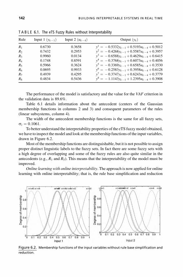
The performance of the model is satisfactory and the value for the VAF criterion in

the validation data is 89.6%.

Table 6.1 details information about the antecedent (centers of the Gaussian

membership functions in columns 2 and 3) and consequent parameters of the rules

(linear subsystems, column 4).

The width of the antecedent membership functions is the same for all fuzzy sets,

si ¼ 0:1061.To better understand the interpretability properties of the eTS fuzzymodel obtained,

we have to inspect themodel and look at themembership functions of the input variables,

drawn in Figure 6.2.

Most of themembership functions are distinguishable, but it is not possible to assign

proper distinct linguistic labels to the fuzzy sets. In fact there are some fuzzy sets with

a high degree of overlapping and some of the fuzzy rules are also quite similar in the

antecedents (e.g., R1 and R5). This means that the interpretability of the model must be

improved.

Online learning with online interpretability. The approach is now applied for online

learning with online interpretability; that is, the rule base simplification and reduction

T A B L E 6.1. The eTS Fuzzy Rules without Interpretability

Rule Input 1 ðyk� 1Þ Input 2 ðuk� 4Þ Output ðykÞR1 0.6730 0.3658 y1 ¼ � 0:5332yk� 1þ 0:5193uk� 4þ 0:5012R2 0.7432 0.2953 y2 ¼ � 0:4268yk� 1þ 0:5587uk� 4þ 0:3957R3 0.9960 0.0134 y3 ¼ � 0:6588yk� 1þ 0:4629uk� 4þ 0:6415R4 0.1748 0.8591 y4 ¼ � 0:3768yk� 1þ 0:6073uk� 4þ 0:4056R5 0.5966 0.3624 y5 ¼ � 0:3369yk� 1þ 0:6585uk� 4þ 0:3530R6 0.0695 0.9933 y6 ¼ � 0:2583yk� 1þ 0:3958uk� 4þ 0:6128R7 0.4939 0.4295 y7 ¼ � 0:3747yk� 1þ 0:6243uk� 4þ 0:3779R8 0.4834 0.5436 y8 ¼ � 1:1143yk� 1þ 1:2395uk� 4þ 0:3908

Figure 6.2. Membership functions of the input variables without rule base simplification and

reduction.


procedures are active during the learning process. The configuration for the online

learning process is basically the same (r ¼ 0:3 and W ¼ diagð750Þ) with the exception

of the new parameter for the similarity threshold between fuzzy sets, l ¼ 0:9. Themerging of similar fuzzy sets takes placewhen the similarity is greater than l. Figure 6.3shows information about the evolution of the online learning process. Table 6.2 contains

Figure 6.3. Online learning process with online interpretability.

T A B L E 6.2. Fuzzy Model Parameters with Online Interpretability

Rule Input 1 ðyk� 1Þ Input 2 ðuk� 4Þ Output ðykÞR1 0.5913 0.5005 y1 ¼ � 0:3760yk� 1þ 0:6276uk� 4þ 0:3743R2 0.9960 0.0134 y2 ¼ � 0:5563yk� 1þ 0:3736uk� 4þ 0:5482R3 0.1748 0.9471 y3 ¼ � 0:3684yk� 1þ 0:6818uk� 4þ 0:2577R4 0.4834 0.5005 y4 ¼ � 0:4271yk� 1þ 0:9937uk� 4þ 0:2577R5 0.0555 0.9471 y5 ¼ � 0:3917yk� 1þ 0:7578uk� 4þ 0:2649


the antecedent and consequent parameters of the eTS fuzzy model acquired from data.

Figure 6.4 presents the membership functions for the input variables at the end of the

learning process. The width of the membership functions is the same as in the previous

experiment, si ¼ 0:1061, since the constant radii remains also the same.

The incorporation of the online rule base simplification and reduction methods

has a large impact over the online learning process. The number of fuzzy rules attains

a maximum of 7 during the learning process and reaches the final number of 5 sooner

than in the previous experiment without online interpretability.

The behavior of the approach is now strongly influenced not only by the parameter

radii but also by the similarity threshold between fuzzy sets. These two parameters allow

the control of the model interpretability, complexity, and precision. The threshold lrepresents the degree towhich the user allows for equality between fuzzy sets used in the

model. The lower the value of l, the more fuzzy sets are merged, decreasing the term set

of the model. It is expected that the numerical accuracy of the model decreases as the

parameter l decreases, but it depends on the redundancy of the model. Typical values

for parameter l are in the range of [0.65, 0.95], but there is always a tradeoff between

accuracy and interpretability, since they act in opposing directions.

The performance of the model is not very different from the one in the previous

experiment. The value for the VAF criterion in the validation data is 89.4%. The reason

for this is that the value for the similarity threshold is quite high, l¼ 0.9. However, the

interpretability of the model has improved considerably since now it is possible to assign

proper linguistic terms to all the fuzzy sets (Figure 6.4). The number of fuzzy rules

reduced from 8 to 5 and for input 2 (uk� 4) the number of linguistic terms necessary to

describe the variable is reduced from 8 to 3. This allows us also to conclude that input 1

(yk� 1) is more relevant than input 2 in the model.

For input 1 (uk-1) the labels are very low, low, medium, quite high, very high. For

input 2 (uk-4) they are very low, medium, very high. With these semantic labels the five

rules are shown in Table 6.3.

Now the time series is verbally described by a set of five rules with semantic

meaning. Of course the fuzzy sets quite high, low, and so on, are those of Figure 6.4 and

no others. For a lower value of the radii coefficient, more rules are obtained, eventually

Figure 6.4. Membership functions of the input variables with online interpretability.


with better performance in the training set but with poorer generalization capabilities in

the testing set. These five rules produce a good value for VAF.

The methodology described in section 6.4, in particular the combination of

supervised subtractive clustering [35, 43] with KRLS [37, 39], has been also applied

to the Box-Jenkins furnace data set. The estimation of relevant data represents an

additional criterion to control machine complexity, that is, nonclustered points will not

be included in the kernel representation [43]. As a result of the application of the KRLS

with clustering, using a Gaussian width of 0.2 and a threshold of 0.01, the number

of kernels achievedwas 8. The representation of themultidimensional fuzzy sets for both

inputs reveals a satisfactory interpretability of the results (Figures 6.5 and 6.6), while the

accuracy has been better than that achieved by the evolving fuzzy system. Comparing the

three proposed methodologies, the KRLS with clustering achieved 95.2% for the VAF

criterion (Table 6.4). Concerning the structure complexity, it is slightly higher than with

Figure 6.5. Representation of the Gaussian kernels as membership functions of the input

variables.

T A B L E 6.3. The Five Interpretable Rules for the Box-Jenkins Time Series Prediction

Rule Syntax

R1 IF uk-1 is quite high AND uk-4 is medium

THEN y1k ¼ � 0:3760yk� 1þ 0:6276uk� 4þ 0:3743R2 IF uk-1 is very high AND uk-4 is very low

THEN y2k ¼ � 0:5563yk� 1þ 0:3736uk� 4þ 0:5482R3 IF uk-1 is low AND uk-4 is very high

THEN y3k ¼ � 0:3684yk� 1þ 0:6818uk� 4þ 0:2577R4 IF uk-1 is medium AND uk-4 is medium

THEN y4k ¼ � 0:4271yk� 1þ 0:9937uk� 4þ 0:2577R5 IF uk-1 is very low AND uk-4 is very high

THEN y5k ¼ � 0:3917yk� 1þ 0:7578uk� 4þ 0:2649


eTSwith online interpretability. However, it should be also noted that the kernelmodel is

equivalent to a zero-order TSK fuzzy systems, while the applied evolving fuzzy system

has linear consequents that help decrease the number of rules. In an overall conclusion,

both methodologies proved to be effective in controlling model complexity, providing a

good tradeoff between interpretability and accuracy.

6.6 CONCLUSION

The approach for online learning with the integration of online rule base simplification

and reduction procedures allows implementing the concept of online transparent

modeling in order to improve interpretability and reduce the complexity of fuzzymodels

acquired with a purely data-driven approach.

The behavior of the approach is strongly influenced by two predefined para-

meters: the radius of the clusters (radii) and the similarity threshold between fuzzy

sets. Parameter radii can be used to control the number of fuzzy rules, and inherently

model complexity and precision, while the similarity threshold parameter can be used

to balance the interpretability and numerical accuracy of the model. These two

parameters together allow the control of model interpretability, complexity, and

precision.

T A B L E 6.4. Structure Complexity Analysis

Method

Structure Complexity

(Number of Rules/Kernels) Accuracy (VAF)

eTS 8 89.6 %

eTS þ Interpretability 5 89.4 %

KRLS þ Clustering 8 95.2 %

Figure 6.6. Time evolution of the number of kernels and norm of the covariance matrix.


The role of the radii of the clusters is also particularly important for the formulation

of different problems concerning the size, shape, and orientation of the clusters. When

the same radii is used for all the input variables of the model, a relatively simple solution

for online transparent modeling can be obtained. The incorporation of the rule base

simplification and reduction methods has a great impact in the online learning process,

and despite the influence of the predefined parameters in the approach iswell understood;

the implications of the merging of fuzzy sets and fuzzy rules in the learning process of

eTS fuzzy models (covariance matrix, consequent parameters, and potential of the

cluster centers) still need to be investigated more deeply.

Procedure (6.16) is a simpleway for knowledge fusion to give satisfactory results for

the presented benchmark problems. However, alternative and more elaborated methods,

for example, the form of an affine combination, might eventually be preferable in other

type of problems. But it must be stated that reestimation of the consequent parameters

in the reduced rule base using past training data is not possible because the data is no

longer available, since we are in the context of online learning, and this is an additional

difficulty that cannot yet be resolved.

The work was developed in the MATLAB environment including the Fuzzy Logic

Toolbox [47].

6.7 ACKNOWLEDGMENTS

The authors express their gratitude to Professor Plamen Angelov, Lancaster University,

for the fruitful and interesting discussions concerning online learning and eTS systems.

This work is supported by the Portuguese Government, under the program PRODEP

III—Acc~ao 5.3, and partially supported by POSI—Programa Operacional Sociedade de

Informac~ao—of Portuguese Fundac~ao para a Ciencia e Tecnologia under Project

ALCINE (POSI/EEI/14155/2001), including FEDEREUfinancial support, and partially

supported by FCT – Fundac~ao para a Ciencia e Tecnologia, under Project BIOINK

(PTDC/EIA/71770/2006).

6.8 REFERENCES

1. D. A. Keim, “Information Visualization and Visual Data Mining,” IEEE Trans. on Visual-

ization and Computer Graphics, 8(1): 1–8, Jan–Mar 2002.

2. P. Angelov, “Evolving Rule-BasedModels: ATool for Design of Flexible Adaptive Systems,”

Studies in Fuzziness and Soft Computing, 92, Springer-Verlag, 2002.

3. N. Kasabov, Q. Song, “DENFIS: Dynamic Evolving Neural-Fuzzy Inference System and Its

Application for Time-Series Prediction,” IEEE Trans. on Fuzzy Systems, 10(2): 144–154,

2002.

4. P.Angelov,D. Filev, “AnApproach toOnline Identification of Takagi-Sugeno FuzzyModels,”

IEEE Trans. on Systems, Man, and Cybernetics—Part B: Cybernetics, 34(1): 484–498, 2004.

REFERENCES 147

5. J. Casillas, O. Cordon, F. Herrera, L. Magdalena, Interpretability Issues in Fuzzy Modeling,

Berlin, Heidelberg: Springer-Verlag, 2003.

6. C. Mencar, G. Castellano, A. M. Fanelli, “Distinguishability Quantification of Fuzzy Sets,”

Information Science, 177: 130–149, Elsevier, 2007.

7. R. Mikut, J. J€akel, L. Gr€oll, “Interpretability Issues in Data-Based Learning of Fuzzy

Systems,” Fuzzy Sets and Systems, 150: 179–197, 2005

8. C. Mencar, G. Castellano, A. M. Fanelli, “Some Fundamental Interpretability Issues in Fuzzy

Modeling.” Proc. EUSFLAT, Barcelona, September 7–9, 2005.

9. M. Setnes, “Complexity Reduction in Fuzzy Systems,” PhD Thesis, Delft University of

Technology, 2001.

10. S.-M. Zhou, J. Q. Gan, “Constructing Accurate and Parsimonious Fuzzy Models with

Distinguishable Fuzzy Sets Based on an Entropy Measure,” Fuzzy Sets and Systems 157:

1057–1074, 2006.

11. E. V. Broekhoven, V. Adriaenssens, B. De Baets, “Interpretability-Preserving Genetic

Optimization of Linguistic Terms in Fuzzy Models for Fuzzy Ordered Classification: An

Ecological Case Study,” Int. J. Approximate Reasoning 44(1): 65–90, 2007.

12. Rafael Alcal�a, Jesus Alcal�a-Fdez, Francisco Herrera, Jos�e Olero, “Genetic Learning of

Accurate and Compact Fuzzy Rule-Based Systems Based on the 2-Tuples Linguistic

Representation,” Int. J. Approximate Reasoning 44(1) (33 ref.): 45–64, 2007, Elsevier, ISSN

0888-613X.

13. C. Sivapragasam, “Rule Reduction in Fuzzy Logic for better Interpretability in Reservoir

Operation Hydrological Processes”, Vol. 21, Issue 21, Hoboken: John Wiley &Sons, 2007,

pp. 2835–2844.

14. J. Gonz�alez, I. Rojas, H. Pomares, L. J. Herrera, A. Guill�en, J. M. Palomares, F. Rojas,

“Improving the Accuracy While Preserving the Interpretability of Fuzzy Function Approx-

imators by Means of Multi-objective Evolutionary Algorithms,” Int. J. Approximate

Reasoning, 44(1): 32–44, 2007.

15. A. F.Gomez-Skarmeta, F. Jim�enez,G. S�anchez, “Improving Interpretability inApproximative

Fuzzy Models via Multiobjective Evolutionary Algorithms,” Int. J. Intelligent Systems, Vol.

22, Issue 9, Wiley Periodicals, 2007, pp. 943–969.

16. H. Ishibuch, Y. Nojima, “Analysis of Interpretability-Accuracy Tradeoff of Fuzzy Systems

byMultiobjective FuzzyGenetics-BasedMachine Learning,” Int. J. Approximate Reasoning,

44(1): 4–31, 2007.

17. J. L. D�ıez, J. L. Navarro, A. Sala, “A Fuzzy Clustering Algorithm Enhancing Local Model

Interpretability,” Soft Computing, A Fusion of Foundations,Methodologies and Applications,

Vol. 11, pp. 973–983, Springer-Verlag, 2007.

18. Feng Liu, Chai Quek, Geok See Ng, “A Novel Generic Hebbian Ordering-Based Fuzzy

Rule Base Reduction Approach to Mamdani Neuro-Fuzzy System,” Neural Comput. 19(6):

1656–80, June 2007.

19. Y. Jin, B. Sendhoff, “Extracting Interpretable Fuzzy Rules from RBF Networks,” Neural

Processing Letters, Vol. 17(2), pp. 149–164 (16), Springer, 2003.

20. M. Eftekhari, S. D. Katebi, M. Karimi, A. H. Jahanmiri, “Eliciting Transparent Fuzzy Model

Using Differential Evolution,” Applied Soft Computing Journal, Elsevier, in press, 2008.

21. E. Lughofer, E. H€ullermeier, E. P. Klement, “Improving the Interpretability of Data-Driven

Evolving Fuzzy Systems.” Proc. EUSFLAT 2005, Barcelona, Spain, 2005, pp. 28–33.


22. K. P. Ajoy, D. Popovic, “Transparent Fuzzy/Neuro-Fuzzy Modelling in Computational

Intelligence in Time Series Forecasting, Theory and Engineering Applications,” London:

Springer, 2005, pp. 275–303.

23. Plamen Angelov, Edwin Lughofer, “Data-Driven Evolving Fuzzy Systems Using eTS and

FLEXFIS: Comparative Analysis,” Int. J. General Systems, 37(1): 45–67, 2008.

24. J. Victor, A. Dourado, “Evolving Takagi-Sugeno Fuzzy Models,” Technical Report, CISUC,

2003, http://cisuc.dei.uc.pt/acg.

25. B. Scholkopf, A. Smola, Learning with Kernels. Cambridge, MA: MIT Press, 2001.

26. V. Vapnik, The Nature of Statistical Learning Theory. Springer, 1995.

27. J. Victor, A. Dourado, “Online Interpretability by Rule Base Simplification and Reduction.”

Proc. Eunite Symposium, Aachen, 2004.

28. J.-S.R. Jang,ANFIS: “Adaptive-Network-Based Fuzzy Inference Systems,” IEEETrans. Syst.

Man Cybern., 23: 665–685, 1993.

29. O. Nelles, “LOLIMOT Local Linear Model Trees for Nonlinear Dynamic System

Identification,” Automatisierungstechnik, 45(4): 163–174, April 1997.


31. P. Angelov, C. Xydeas, “Fuzzy Systems Design: Direct and Indirect Approaches,” Soft

Computing: A Fusion of Foundations, Methodologies and Applications, 10: 836–849,

Springer Verlag, 2006.

32. M. Setnes, R. Babuska, U. Kaymak, H. R. van Nauta Lemke, “Similarity Measures in

Fuzzy Rule Base Simplification,” IEEE Trans. on Systems, Man, and Cybernetics—Part

B: Cybernetics, 28(3): 376–386, 1988.

33. Y. Jin, “FuzzyModeling of High-Dimensional Systems: Complexity Reduction and Interpret-

ability Improvement,” IEEE Trans. on Fuzzy Systems, 8(2): 212–221, 2000.

34. A. Bordes, S. Ertekin, J.Weston, L�eonBottou, “Fast Kernel Classifiers withOnline andActiveLearning,” J. Machine Learning Research, 6: 1579–1619, 2005.

35. G. Cauwenberghs, T. Poggio, “Incremental and Decremental Support Vector Machine

Learning.” In Advances in Neural Processing Systems, vol. 10, Cambridge, MA: MIT Press,

USA, 2001.

36. C. Diehl, G. Cauwenberghs, “SVM Incremental Learning, Adaptation and Optimization.”

Proc. IEEE Int. Joint Conf. Neural Networks (IJCNN’03), 2003.

37. Y. Engel, S. Mannor, R. Meir, “The Kernel Recursive Least Squares Algorithm,” IEEE Trans.

Signal Proc., 52(8): 2275–2285, 2004.

38. T. Ahmed, M. Coates, A. Lakhina, “Multivariate Online Anomaly Detection Using Kernel

Recursive Least Squares.” Proc. IEEE Infocom, Anchorage, 2007.

39. D. Wingate, S. Singh, “Kernel Predictive Linear Gaussian Models for Nonlinear Stochastic

Dynamical Systems.” Int. Conf. Machine Learning, 2006; resources at web.mit.edu/wingated/www/resources.html.

40. S. Van Vaerenbergh, J. Vıa, I. Santamarıa, “A Sliding Window Kernel RLS Algorithm and Its

Application to Nonlinear Channel Identification.” IEEE Int. Conf. Acoustics, Speech, and

Signal Processing (ICASSP), Toulouse, France, May 2006.

41. T. Runarsson, S. Sigurdsson, “Asynchronous Parallel Evolutionary Model Selection for

Support Vector Machines,” Neural Information Processing—Letters and Reviews, 3(3):

59–67, 2004.

REFERENCES 149

42. C. Cortes, V. Vapnik, “Support Vector Networks,” Machine Learning, 20: 273–297, 1995.

43. C. Pereira, A. Dourado, “On the Complexity and Interpretability of Support Vector Machines

for Process Modeling. IJCNN ’02—Int. Joint Conference on Neural Networks, 2002.

44. N. Barakat, J. Diederich, “Eclectic Rule-Extraction from Support Vector Machines,” Int. J.

Computational Intelligence, 2(1): 59–62, 2005.

45. R. Yager, D. Filev, “Learning of Fuzzy Rules by Mountain Clustering.” Proc. SPIE Conf. on

Applications of Fuzzy Logic Technology, Boston, 1994, pp. 246–254.

46. UCIRepository ofMachine LearningDatabases, University of California, www.ics.uci.edu/mlearn/MLRepository.html.

47. MATLAB and Fuzzy Logic Toolbox, Mathworks, Inc.


7

ONLINE FEATURE EXTRACTIONFOR EVOLVING INTELLIGENT

SYSTEMSS. Ozawa, S. Pang, N. Kasabov

7.1 INTRODUCTION

Whenwe build a classification systemor a forecasting system,we sometimes encounter a

situation where it is not easy to collect a complete set of training samples. For example,

human faces have large variations due to lighting conditions, emotional expression,

glasses, makeup, hairstyles, age, and so forth. Taking all these factors into consideration

when a face database is constructed is almost impossible. Thus, in many cases, we

construct an imperfect system that workswell in some limited conditions, and the system

is improved whenever the system makes incorrect recognition or prediction. Therefore,

inmore practical situations, the presentation of training samples becomes sequential, and

the learning and prediction have to be alternatively carried out by a system. This type of

learning is often called online learning. On the other hand, in some practical applications

(e.g., stock price forecasting), the property of a data source might be changed over time.

In that case, even if a system made a correct prediction for some input at a certain time,

the prediction might have to be modified in the future. Then, the learning also has to be

online. In online learning circumstances, a system is required to modify only wrong

predictions without loosing prediction accuracy for other inputs. In this sense, incre-

mental learning has recently received a great deal of attention in many practical

applications.

When data are composed of many attributes, feature extraction (or selection) is very

important to attain both good generalization performance and fast learning of classifiers.


and Nikola Kasabov


Therefore, the incremental learning should be considered not only for classifiers but also

for feature extraction. However, many approaches to incremental learning are aimed at

classifiers such as decision trees (Utgoff, 1989; Weng & Hwang, 2007), support vector

machines (Shilton et al., 2005), memory-based learning models (Atkeson, 1997), and

neural networks (Carpenter & Grossberg, 1988). There have not been proposed many

incremental feature extraction methods so far.

As for the incremental learning of feature extraction, Incremental Principal Com-

ponent Analysis (IPCA) (Hall et al., 1998; Oja & Karhunen, 1985, Sanger, 1989) and

Incremental Linear Discriminant Analysis (ILDA) (Weng et al., 2003) have been

proposed. Hall and Martin (1998) have devised a smart method to update eigenvectors

and eigenvalues incrementally based on eigenvalue decomposition. Ozawa et al. (2004)

have extended this IPCA algorithm such that an eigen-axis is augmented based on the

accumulation ratio in order to control the dimensionality of an eigenspace easily. On the

other hand, Pang et al. (2005) have proposed an incremental LDA (ILDA) algorithm in

which a between-class scatter matrix and a within-class scatter matrix are incrementally

updated, and then the eigen-axes of a feature space are obtained by solving an

eigenproblem. Zhao et al. (2006) have also proposed different ILDA algorithms based

on a singular decomposition technique.

Recently, we have proposed a new scheme of incremental learning in which

feature extraction and classifier learning are simultaneously carried out online

(Ozawa et al., 2004, 2005; Pang et al., 2005). In our previous work, IPCA or ILDA

are adopted as feature extraction methods, and k-nearest neighbor classifier with

Evolving Clustering Method (ECM) (Kasabov, 2002) or Resource Allocating

Network with Long-Term Memory (RAN-LTM) (Kobayashi et al., 2001; Ozawa

et al., 2005) are adopted as classifiers. A distinctive feature of the proposed scheme

is that the learning of feature extraction and a classifier is simultaneously conducted in

one pass, which means that training samples are passed through a system only once

for learning purposes (Kasabov, 2002). One-pass incremental learning is quite

important and effective especially when a system has to learn from a large-scale data

set with limited computational resources (i.e., CPU performance and memory). It

was verified that the classification accuracy of the above classification system

was improved constantly even if a small set of training samples were provided at a

starting point (Ozawa et al., 2005). To enhance the learning speed, we have proposed an

extension of IPCA (Ozawa et al., 2008), called Chunk IPCA, in which the update of an

eigenspace is completed for a chunk of data by performing single eigenvalue

decomposition.

This chapter introduces the above two versions of IPCA as online feature extraction

methods and shows how to construct a classification system. Section 7.2 describes the

learning algorithm of IPCA in which an eigenspace model is updated for a single

training sample at a time. Section 7.3 explains Chunk IPCA, which can update an

eigenspace model with a chunk of training samples; in addition, we explain how to

combine IPCAwith k-nearest neighbor classifier, whose prototypes are trained by ECM.

In section 7.4, we show the performance evaluation for IPCA and Chunk IPCA using

six real data sets. Section 7.5 summarizes the chapter and discusses directions for

further work.

152 ONLINE FEATURE EXTRACTION FOR EVOLVING INTELLIGENT SYSTEMS

7.2 INCREMENTAL PRINCIPAL COMPONENT ANALYSIS (IPCA)

7.2.1 Learning Assumptions and General Idea in IPCA

Assume thatN training samples xðiÞ 2 Rnði ¼ 1; . . . ;NÞ are initially provided to a systemand an eigenspace model W ¼ ð�x;Uk;Lk;NÞ is obtained by applying Principal Com-

ponent Analysis (PCA) to the training samples. In the eigenspace model W, �x is a mean

vector of xðiÞði ¼ 1; . . . ;NÞ, Uk is an n k matrix whose column vectors correspond to

eigenvectors, andLk ¼ diag l1; . . . ;lkf g is a k kmatrix whose diagonal elements are

non-zero eigenvalues. Here, k is the number of eigen-axes spanning the eigenspace (i.e.,

eigenspace dimensionality) and the value of k is determined based on a certain criterion

(e.g., accumulation ratio). After calculating W, the system holds the information on Wand all the training samples are thrown away.

Now assume that the ðNþ 1Þth training sample xðNþ 1Þ ¼ y 2 Rn is given. The

addition of this new sample results in the changes in the mean vector and the covariance

matrix; therefore, the eigenspace model W ¼ ð�x;Uk;Lk;NÞ should be updated. Let us

define the new eigenspacemodel byW0 ¼ ð�x0;U0k0 ;L0k0 ;Nþ 1Þ. Note that the eigenspacedimensions might be increased from k to k þ 1; thus, k0 in W0 is either k or k þ 1.

Intuitively, if y includes almost all energy in the current eigenspace spanned by the

eigenvectors U0k, there is no need to increase its dimensions. However, if y includes

certain energy in the complementary eigenspace, the dimensional augmentation is

inevitable; otherwise, crucial information on the new sample ymight be lost. Regardless

of thenecessity ineigenspaceaugmentation, theeigen-axesshouldberotated toadapt to the

variation in the data distribution. In summary, there are three main operations in IPCA:

(1) mean vector update, (2) eigenspace augmentation, and (3) rotation of eigen-axes.

The first operation is easily carried out based on the following equation:

�x0 ¼ 1

Nþ 1ðN�xþ yÞ 2 Rn ð7:1Þ

The other two are explained below.

7.2.2 Condition on Eigenspace Augmentation

There are two criteria for decidingwhether the dimensional augmentation is needed.One

is the norm of a residue vector defined by

h ¼ ðy��xÞ�UTkg where g ¼ UT

k ðy��xÞ ð7:2ÞHere, T means the transposition of vectors and matrixes. The other is the accumulation

ratio whose definition and incremental calculation are shown as follows:

AðUkÞ ¼

Xki¼1

li

Xnj¼1

lj¼ðNþ 1Þ

Xki¼1

li þ jUTk ðy��xÞ

j2ðNþ 1Þ

Xnj¼1

lj þ jy��xj jj2ð7:3Þ

INCREMENTAL PRINCIPAL COMPONENT ANALYSIS (IPCA) 153

where li is the ith largest eigenvalues, and n and kmean the dimensionality of the input

space and that of the current eigenspace, respectively. The former criterion in equa-

tion (7.2) was adopted by the original IPCA proposed by Hall andMartin (1998), and the

latter in equation (7.3) was used in the modified IPCA proposed by the authors (Ozawa

et al., 2004). Using these criteria, the condition on the eigenspace augmentation is

respectively represented by:

½Residue Vector Norm� h ¼ h= jhj jj if jhj jj>h0 otherwise

�ð7:4Þ

½Accumulation Ratio� h ¼ h= jhj jj if AðUkÞ < q0 otherwise

�ð7:5Þ

where h (in the original IPCA (Hall &Martin, 1998), h is set to zero) and q are a positiveconstant. Note that setting a too-large threshold h or too-small q would cause serious

approximation errors for eigenspacemodels.Hence, it is important to set proper values to

h in equation (7.4) and q in equation (7.5). In general, finding a proper threshold h is

easier than doing a proper q unless input data are appropriately normalized within a

certain range (another difficulty arises for automatic data normalization in online

learning environments). On the other hand, since the accumulation ratio is defined by

the ratio of input energy in an eigenspace over the original input space, the value of q isrestricted between 0 and 1. Therefore, it would be easier for q to get an optimal value by

applying a cross-validationmethod. The detailed algorithm of selecting q in incremental

learning settings is described in Ozawa et al. (2008).

7.2.3 Eigenspace Rotation

If the condition of equation (7.4) or (7.5) satisfies, the dimensions of the current

eigenspace would be increased from k to kþ 1, and a new eigen-axis h should be

added to the eigenvector matrix Uk. Otherwise, the dimensionality remains the same.

After this operation, the eigen-axes are rotated to adapt to the new data distribution.

Assume that the rotation is given by a rotation matrix R; then the eigenspace update is

represented by the following equation:

1. If there is a new eigen-axis to be added,

U0kþ 1 ¼ ½Uk; h�R ð7:6Þ

2. Otherwise,

U0k ¼ UkR ð7:7Þ

In order to obtain R, it has been shown that new eigenvectors and the corresponding

eigenvalues are obtained by solving the following intermediate eigenproblem (Hall &

Martin, 1998):


1. If there is a new eigen-axis to be added,

N

N þ 1

Lk 0

0T 0

� �þ N

ðNþ 1Þ2ggT ggggT g2

� �( )R ¼ RL0kþ 1 ð7:8Þ

2. Otherwise,

N

Nþ 1Lk þ N

ðNþ 1Þ2 ggT

( )R ¼ RL0k ð7:9Þ

Here, g ¼ hðy��xÞ and 0 is a k-dimensional zero vector. Here,L0kþ 1 andL0k are the neweigenvalue matrixes whose diagonal elements correspond to k and kþ 1 eigenvalues,

respectively. Using the solutionR, the new eigenvectormatrixU0k orU0kþ 1 is calculated

from equation (7.6) or (7.7).

7.3 CHUNK INCREMENTAL PRINCIPAL COMPONENT ANALYSIS(CIPCA)

IPCA can be applied to a single training sample at a time, and the intermediate

eigenproblem in equation (7.8) or (7.9) must be solved separately for each of the

samples even though a chunk of samples is provided for learning. Obviously, this is

inefficient from a computational point of view, and the learning may get stuck in a

deadlock if a large chunk of training samples is given to learn in a short time. That is, the

next chunk of training samples could come before the learning is completed if it takes a

long time to update an eigenspace.

To overcome this problem, we extended the original IPCA so that the eigenspace

model W can be updated with a chunk of training samples in a single operation (Ozawa

et al., 2008). This extended algorithm is called Chunk IPCA.

7.3.1 Update of Eigenspace

Let us assume that training samplesX ¼ xð1Þ; . . . ; xðNÞ� � 2 RnN have been given so far

and they were already discarded. Instead of keeping actual training samples, a system

holds an eigenspace model W ¼ ð�x;Uk;Lk;NÞ where �x, Uk, and Lk are a mean input

vector, an n k eigenvector matrix, and a k k eigenvaluematrix, respectively. Here, k

is the number of eigen-axes spanning the current eigenspace. Now, assume that a chunk

of L training samples Y ¼ yð1Þ; . . . ; yðLÞ� � 2 RnL is presented. The mean vector �x0 is

updated without the past training samples X as follows:

�x0 ¼ 1

N þ LN�xþ L�yð Þ ð7:10Þ

Next, let us derive the update equations forUk andLk. Suppose that l eigen-axes are

augmented to avoid loosing essential input information when a chunk of L training

CHUNK INCREMENTAL PRINCIPAL COMPONENT ANALYSIS (CIPCA) 155

samples Y is provided; that is, the eigenspace dimensions are increased by l. Let us

denote the augmented eigen-axes as follows:

Hl ¼ fh1; . . . ; hlg 2 Rnl ; 0 � l � L ð7:11Þ

Then, the updated eigenvector matrix U0kþ l is represented by

U0kþ l ¼ ½Uk;Hl �R ð7:12Þ

where R is a rotation matrix. It has been shown that eigenvectors and the corresponding

eigenvalue are obtained by solving the following intermediate eigenproblem (Ozawa et

al., 2008):

1. If there are new eigen-axes to be added (i.e., l 6¼ 0),

N

N þ L

Lk 0

0T 0

" #þ NL2

ðNþ LÞ3�g�gT �g�gT

�ggT �g�gT

" #þ N2

ðN þ LÞ3XLi¼1

g0ig0iT g0ig 0

Ti

g 0ig0iT g 0ig 0

Ti

" #(

LðLþ 2NÞðNþ LÞ3

XLi¼1

g00ig00i

Tg00ig00Ti

g 00ig00i

T g 00ig00Ti

" #)R ¼ RL0kþ l ð7:13Þ

2. Otherwise,

N

NþLLkþ NL2

ðNþLÞ3�g�gTþ N2

ðNþLÞ3XLi¼1

g0ig0Ti þ

LðLþ2NÞðNþLÞ3

XLi¼1

g00ig00Ti

( )R¼RL0k

ð7:14Þ

where �g¼UTk ð�y��xÞ, g0i¼UT

k ðyðiÞ��xÞ, g00i¼UT

k ðyðiÞ��yÞ, �g¼HTl ð�y��xÞ,

g 0i¼HTl ðyðiÞ��xÞ, g

00i¼HT

l ðyðiÞ��yÞ.

Solving this intermediate eigenproblem, the rotation matrix R and the eigenvalue

matrix L0kþ l are obtained. Then, the corresponding new eigenvector matrix U0kþ l is

given by equation (7.12).

7.3.2 A Criterion for Eigen-axis Augmentation

In Chunk IPCA, the number of eigen-axes to be augmented is determined by finding the

minimum k such that AðUkÞ � q holds where q is a threshold between 0 and 1. To

introduce this criterion, we need to modify equation (7.3) such that the accumulation

ratio can be updated incrementally for a chunk of L samples. In Chunk IPCA, we need

two types of accumulation ratios. One is the accumulation ratio for a k-dimensional

eigenspace spanned by U0k ¼ UkR and the other is that for a (k þ l)-dimensional


augmented eigenspace spanned by U0kþ l ¼ Uk Hl½ �R. The former is used for checking

whether the current k-dimensional eigenspace should be augmented. The latter is used

for checking whether further eigen-axes are needed for the (k þ l)-dimensional aug-

mented eigenspace.

The updated accumulation ratio A0ðU0kÞ and A0ðU0kþ lÞ are calculated as follows:

A0ðU0kÞ ¼

Xki¼1

li þ L

Nþ Lj�gj jj2þ 1

N

XLj¼1

��g00 j��2Xni¼1

li þ L

N þ Lj�mj jj2þ 1

N

XLj¼1jm00 j j2

ð7:15Þ

A0ðU0kþ lÞ �

Xki¼1

li þ L

N þ L

�� g�g��2þ 1

N

XLj¼1

�� g00 jg 00 j

��2Xni¼1

li þ L

Nþ Lj�mj jj2þ 1

N

XLj¼1

��m00 j��2ð7:16Þ

where �m ¼ �x��y and m00 j ¼ yðjÞ��y. To update A0ðU0kÞ, the summation of eigenvalues

liði ¼ 1; . . . ; nÞ is required, and this summation can be held by accumulating the power

of training samples. Hence, the individual eigenvalues li (i ¼ kþ 1; . . . ; n) are not

necessary for this update. As seen from equations (7.15) and (7.16), we need no past

sample xðjÞ and no rotation matrix R to update the accumulation ratio. Therefore, this

accumulation ratio is updated with the following information: a chunk of given training

samples Y ¼ fyð1Þ; . . . ; yðLÞg, the current eigenspace model W ¼ ð�x;Uk;Lk;NÞ, thesummation of eigenvalues

Xni¼1

li, and a set of augmented eigen-axes Hl , which are

obtained through the procedure described next.

7.3.3 Selection of Eigen-axes

In IPCA, a new eigen-axis is selected so as to be perpendicular to the existing

eigenvectors given by the column vectors of Uk. A straightforward way to get new

eigen-axes is to apply Gram-Schmidt orthogonalization to a chunk of given training

samples (Hall et al., 2000). If the training samples are represented by ~L linearly

independent vectors, the maximum number of augmented eigen-axes is ~L. However,the subspace spanned by all of the ~L eigen-axes is redundant in general; in addition,

if the chunk size is large, the computation costs to solve the intermediate eigenproblem

in equation (7.13) would be considerably expensive. Therefore, we need to find the

smallest set of eigen-axes without losing essential information of the given training

samples.


The problem of finding an optimal set of eigen-axes is stated below.

Find the smallest set of eigen-axes H* ¼ fh1; . . . ; hl*g for the current eigenspacemodel W ¼ ð�x;Uk;Lk;NÞ without keeping the past training samples X such that

the accumulation ratio A0ðU0kþ l*Þ of the given training samples fX;Yg is largerthan a threshold q.

Assume that we have a candidate set of augmented eigen-axes Hl ¼ fh1; . . . ; hlg.Since the denominator of equation (7.16) is constant once themeanvector �y is calculated,the increment of the accumulation ratio from A0ðU0kÞ to A0ðU0kþ lÞ is determined by the

numerator terms. Thus, let us define the following difference D ~A0 ðU0kþ lÞ of the

numerator terms between A0ðU0kÞ and A0ðU0kþ lÞ:

D ~A0 ðU0kþ lÞ ¼ L

Nþ L

��HTl ð�x��yÞ

��2þ 1

N

XLj¼1

��HTl ðyðjÞ��yÞ

��2defXli¼1

D~A0i ð7:17Þ

where

D~A0i ¼ L

Nþ LfhTi ð�x��yÞg

2þ 1

N

XLj¼1fhTi ðyðjÞ��yÞg

2 ð7:18Þ

Equation (7.17) means that the increments of the accumulation ratio are determined by

the linear sum of D~A0i. Therefore, to find the smallest set of eigen-axes, first find hi with

the largest D~A0i, and put it into the set of augmented eigen-axes Hl (i.e., l ¼ 1 and

Hl ¼ hi). Then, check whether the accumulation ratio A0ðU0kþ lÞ in equation (7.16)

becomes larger than the threshold q. If not, select hi with the second-largestD ~A0 i, and thesame procedure is repeated until A0ðU0kþ lÞ � q satisfies. This type of greedy algorithm

makes the selection of an optimal set of eigen-axes very simple. Eigen-axis selection is

summarized in Pseudo-code 1.

Pseudo-code 1: Selection of Eigen-axes

Input: Eigenspace model W ¼ ð�x;Uk;Lk;NÞ, a chunk of L training samples

Y ¼ fyð1Þ; . . . ; yðLÞg, the summation of eigenvaluesPn

i¼1 li, and threshold q of accumu-

lation ratio.

1. Calculate the mean vector �y of the given training samples Y.

2. Calculate the accumulation ratio A0ðU0kÞ from equation (7.15).

3. If A0ðU0kÞ � q, terminate this algorithm.

4. For i ¼ 1 to L do

Obtain the following residue vectors hi using the ith training sample yðiÞ:

hi ¼ ri

jrij jj where ri ¼ ðyðiÞ��xÞ�UkU

Tk ðyðiÞ��xÞ: ð7:19Þ

End for


5. Define an index set G of hi, and initialize H and l.

6. Loop:

(i) Find the residue vector hi0 that gives the largest D ~A0 i in equation (7.18):

hi0 ¼ argmaxi2G D~A0i.

(ii) H ½H; hi0 �, l lþ 1, and G G�i0.(iii) If G is empty, terminate this algorithm.

(iv) Calculate the updated accumulation ratio A0ðU0kþ lÞ from equation (7.16).

(v) If A0ðU0kþ lÞ>q, terminate this algorithm.

End loop

Output: Set of augmented eigen-axes: Hl ¼ fh1; . . . ; hlg.

7.3.4 Training of Initial Eigenspace

Assume that a set of initial training samples D0 ¼ fðxðiÞ; zðiÞÞji ¼ 1; . . . ;Ng is given

before the learning gets started. To obtain an initial eigenspace model

W ¼ ð�x;Uk;Lk;NÞ, the conventional PCA is applied to D0 and the smallest dimension-

ality k of the eigenspace is determined such that the accumulation ratio is larger than q.Since a proper q is usually unknown and often depends on training data, the cross-

validation technique can be applied to determining q (Ozawa et al., 2008).However, let usassume that a proper q is given in advance. The initial training is shown in Pseudo-code 2.

Pseudo-code 2: Training of Initial Eigenspace

Input: Initial training set D0 ¼ fðxðiÞ; zðiÞÞji ¼ 1; . . . ;Ng and threshold q.1. Calculate the mean vector �x of xðiÞ 2 D0.

2. Apply PCA to D0 and obtain the eigenvectors Un ¼ fu1; . . . ; ung whose eigenvalues

Ln ¼ diagfl1; . . . ; lng are sorted in decreasing order.

3. Find the smallest k such that the following condition holds: AðUkÞ � q.Output: W ¼ ð�x;Uk;Lk;NÞ where Uk ¼ fu1; . . . ; ukg and Lk ¼ diagfl1; . . . ; lkg.

7.3.5 Incremental Learning of a Classifier

Since the eigen-axes spanning a feature space are rotated and sometimes increased

over time, it is not simple to build a classifier under such a dynamic environment.

For this purpose, we have proposed a nearest-neighbor classifier whose prototypes

(reference vectors) are evolved by the Evolving Clustering Method (ECM)

(Kasabov, 2002).

Let the jth prototype in the current eigenspace W ¼ ð�x;Uk;Lk;NÞ be~pjðj ¼ 1; . . . ;PÞ and let the corresponding prototype in the original input space be


pj . Here, P is the number of prototypes. Obviously, the following relation holds between

these prototypes:

~pj ¼ UTk ðpj��xÞ ð7:20Þ

After adding a chunk of L training samplesY, assume that the eigenspaceW is updated to

W0 ¼ ð�x0;U0ðkþ lÞ;L0ðkþ lÞ;Nþ LÞ. Substituting equations (7.10) and (7.12) into (7.20),

the updated prototypes ~p0jðj ¼ 1; . . . ;PÞ are given by

~p0j ¼ U0Tðkþ lÞðpj��x0Þ ¼ RT~pj

HTðpj��xÞ� �

þ L

N þ LRT �g

�g

� �ð7:21Þ

If no dimensional augmentation is needed,H ¼ 0 holds. Hence, equation (7.21) reducesto

~p0j ¼ RT~pj þL

N þ LRT�g ð7:22Þ

where no information on pj is needed in the prototype update. However, when the

dimensional augmentation as well as the rotation occurs, the original prototypes pj are

necessary for the exact calculation of the new prototype ~p0j . That is, unless we keep theoriginal prototypes in memory, it is impossible to carry out this prototype update.

Since the complementary space generally includes only negligible energy of the

prototypes, equation (7.21) is approximated by

~p0j � RT ~pj0

� �þ L

N þ LRT �g

�g

� �ð7:23Þ

where ½~pTj ; 0T �T is a (k þ 1)-dimensional columnvector that is given by adding l zeros to

the current prototype ~pj . This approach is efficient in memory use, but we have to mind

the approximation error if the threshold q is too small.

7.3.6 Incremental Learning Algorithm

In online learning environments, classification and learning in a system are conducted

alternatively as follows. First, suppose thatN training samples are given to form an initial

eigenspace modelW ¼ ð�x;Uk;Lk;NÞ. Then, a chunk of query inputs is presented to thesystem, and the distances between each of the query inputs and all the prototypes are

calculated, and then the nearest-neighbor method is applied to determine the class. The

misclassified query inputs (and sometimes some of the correctly classified ones) as well

as their class labels are stored temporally into a set of training samples

Y ¼ fyð1Þ; . . . ; yðLÞg where L is the number of training samples. Next, Y is applied to

Chunk IPCA to update the current eigenspace modelW. The updated eigenspace model

W0 ¼ ð�x0;U0ðkþ lÞ;L0ðkþ lÞ;Nþ LÞ is utilized for transformingY into the features, and the

feature vectors as well as the prototypes are used to train the classifier.


The main routine for learning and classification is summarized in Pseudo-code 3.

Note that the online classification process to select a set of training samplesY is omitted

here for the sake of simplicity.

Pseudo-code 3: Learning and classification

Input: Initial training set D0 ¼ fðxðiÞ; zðiÞÞji ¼ 1; . . . ;Ng and the threshold q of accu-

mulation ratio.

Initialization:

1. Call Training of Initial Eigenspace to calculate the initial eigenspace model

W ¼ ð�x;Uk;Lk;NÞ of D0 ¼ fðxðiÞ; zðiÞÞji ¼ 1; . . . ;Ng.2. Calculate the projection of each initial training sample xðiÞ 2 D0 into the eigenspace to

obtain the feature vector ~xðiÞ. Apply ECM (Kasabov, 2002) to the feature vectors, and

obtain the prototypes ~pj .

3. Loop:

(i) Input: A new chunk of training samples D ¼ fðyðiÞ; zðiÞÞji ¼ 1; . . . ; Lg.(ii) Apply Chunk IPCA to Y ¼ fyð1Þ; . . . ; yðLÞg:

(a) Call Selection of Eigen-axes to obtain Hl of the l augmented eigen-axes.

(b) Solve an intermediate eigenproblem in equation (7.13) or (7.14) to obtain a

rotation matrix R and an eigenvalue matrix L0kþ l .

(c) Update the mean vector �x0 and the eigenvector matrix U0kþ l based on

equations (7.10) and (7.12), respectively.

(iii) Update the eigenspace model as follows: W ¼ ð�x;Uk;Lk;NÞ W0 ¼ð�x0;U0ðkþ lÞ;L0ðkþ lÞ;Nþ LÞ.

(iv) Calculate the feature vectors ~Y ¼ f~yð1Þ; . . . ; ~yðLÞg of Y as follows:

~yðiÞ ¼ U0hðyðiÞ��xÞ ði ¼ 1; . . . ; LÞ.(v) Apply ECM to ~Y, and obtain the updated prototypes ~p0 jðj ¼ 1; . . . ;PÞwhere P is

the number of prototypes.

(vi) Predict the classes of yðiÞði ¼ 1; . . . ; LÞ based on the nearest-neighbor method.

Output: Prediction zðyðiÞÞði ¼ 1; . . . ; LÞ.End loop

7.4 PERFORMANCE EVALUATION

7.4.1 Experimental Setup

We selected six data sets for evaluation from the UCI Machine Learning Repository

(see Table 7.1), which have various numbers of data samples and attributes. Since

Internet Advertisement, MUSK, and Spambase are not divided into training and test

samples, we split them randomly into two halves, and the evaluations are conducted

based on twofold cross-validation. Although, theMUSKdatabase includes two data sets,

we select the larger one.

PERFORMANCE EVALUATION 161

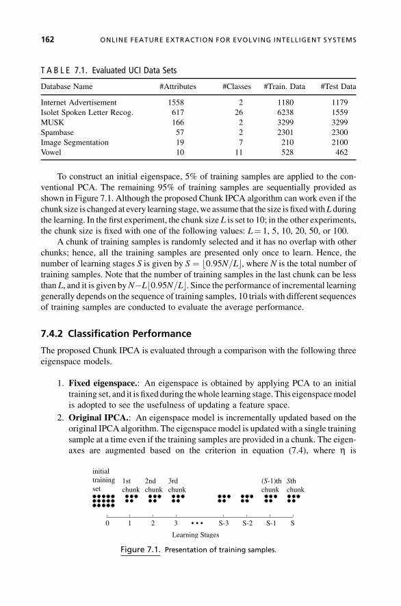
To construct an initial eigenspace, 5% of training samples are applied to the con-

ventional PCA. The remaining 95% of training samples are sequentially provided as

shown in Figure 7.1. Although the proposed Chunk IPCA algorithm can work even if the

chunk size is changed at every learning stage,we assume that the size is fixedwithL during

the learning. In the first experiment, the chunk size L is set to 10; in the other experiments,

the chunk size is fixed with one of the following values: L¼ 1, 5, 10, 20, 50, or 100.

A chunk of training samples is randomly selected and it has no overlap with other

chunks; hence, all the training samples are presented only once to learn. Hence, the

number of learning stages S is given by S ¼ 0:95N=Lb c, where N is the total number of

training samples. Note that the number of training samples in the last chunk can be less

than L, and it is given byN�L 0:95N=Lb c. Since the performance of incremental learning

generally depends on the sequence of training samples, 10 trials with different sequences

of training samples are conducted to evaluate the average performance.

7.4.2 Classification Performance

The proposed Chunk IPCA is evaluated through a comparison with the following three

eigenspace models.

1. Fixed eigenspace.: An eigenspace is obtained by applying PCA to an initial

training set, and it is fixedduring thewhole learning stage. This eigenspacemodel

is adopted to see the usefulness of updating a feature space.

2. Original IPCA.: An eigenspace model is incrementally updated based on the

original IPCA algorithm. The eigenspace model is updated with a single training

sample at a time even if the training samples are provided in a chunk. The eigen-

axes are augmented based on the criterion in equation (7.4), where h is

T A B L E 7.1. Evaluated UCI Data Sets

Database Name #Attributes #Classes #Train. Data #Test Data

Internet Advertisement 1558 2 1180 1179

Isolet Spoken Letter Recog. 617 26 6238 1559

MUSK 166 2 3299 3299

Spambase 57 2 2301 2300

Image Segmentation 19 7 210 2100

Vowel 10 11 528 462

3210

initialtrainingset

1stchunk

2ndchunk

3rdchunk

Learning Stages

SS-1S-2S-3

Sthchunk

(S-1)thchunk

Figure 7.1. Presentation of training samples.


determined such that the eigenspace has similar dimensionality to the eigenspace

constructed by the proposed Chunk IPCA. Therefore, the main concern in

adopting the original IPCA is to evaluate the computation costs.

3. Batch PCA.: An eigen-feature space is updated at every learning stage by

applying PCA to all the training samples given so far. The computation costs

would bemore expensive than the incremental learning methods, but an accurate

eigenspace is always obtained. The dimensionality of an eigenspace is set to the

same value as the proposed Chunk IPCA. Therefore, the classification accuracy

of this method gives a target value for the proposed Chunk IPCA.

Table 7.2 shows the experimental results of the above three eigenspace models and

the proposed Chunk IPCA (L¼ 10) when the nearest neighbor method combined with

ECM is adopted as classifier. As seen in Table 7.2a, the classification accuracy of the

fixed eigenspace model is inferior to other models except for the Isolet and MUSK data

sets. This result shows that the features extracted from the initial training samples were

inappropriate to classify the remaining training samples correctly; therefore, it is

effective to update the feature space to adapt to the change of data distributions. As

for the Isolet and MUSK data sets, we could not find a clear difference in classification

accuracy, and the results suggest that even 5% of training samples include enough

information to construct an effective eigenspace. However, even in such a case, the

importance of incremental learning is not lost because it is generally impossible to know

in advance whether an initial data set includes a sufficient amount of information on

future training samples.

On the other hand, there is no significant difference in classification accuracy

between the original IPCA and the Chunk IPCA. This is not a negative result because the

thresholdh in equation (7.4) is determined such that the eigenspaces constructed by these

T A B L E 7.2. Performance Comparison on (a) Classification Accuracy and (b) CPU Time withThree Eigenspace Models: Fixed Eigenspace, Original IPCA, and Batch IPCA

(a) Classification Accuracy

Advertisement Isolet MUSK Spambase Segmentation Vowel

Fixed Eigenspace 89.7 88.0 95.0 69.4 77.3 54.8

Original IPCA 93.2 88.3 95.1 78.9 87.3 57.7

Batch PCA 94.2 88.5 94.8 79.2 87.3 58.6

Chunk IPCA 93.4 88.0 94.9 78.9 87.3 57.2

(b) CPU Time

Advertisement Isolet MUSK Spambase Segmentation Vowel

Fixed Eigenspace 13.7 1.8 0.044 0.003 0.0003 0.001

Original IPCA 18.1 6379 17.4 27.4 0.073 0.109

Batch PCA 3000 2146 37.6 3.1 0.022 0.05

Chunk IPCA 18.5 265.9 1.7 0.9 0.023 0.058


two models have as similar a dimensionality as possible; that is, the threshold value is

determined such that the two eigenspaces include the same amount of information on

training samples. Compared with the Batch PCA, the proposed Chunk IPCA has slightly

lower classification accuracy; however, the difference is not significant. This means that

the proposed method ensures the quasi-optimality in the construction of eigenspace

without keeping past training samples.

The computation costs of the eigenspace update are estimated by measuring the

CPU time using a MATLAB function. In Table 7.2b, the CPU time of Fixed Eigenspace

corresponds to the time required to construct an initial feature space. As you can see in

Table 7.2b, the computation costs of Chunk IPCA are significantly reduced against both

Original IPCA and Batch PCA, especially for large data sets. However, for the

Advertisement data set, Chunk IPCA has no advantage over Original IPCA, in which

an intermediate eigenproblem is solved for every training sample. The main reason for

this is that the computation costs of the eigen-axis selection could be expensive for large-

dimensional data because the large-scale matrix multiplication is neededmany times for

all eigen-axis candidates. However, this can be alleviated by introducing a more

sophisticated search algorithm (e.g., binary search) in the eigen-axis selection. The

experimental results here suggest that the proposed method possesses excellent scal-

ability unless the number of attributes is too large.

7.4.3 Influence of Chunk Size on System Performance

Since eigen-axes selection is based on a greedy approach, the approximation error of

eigen-axes obtained by Chunk IPCA could increase when a large chunk of training

samples is given for training at one time.On the other hand, fast learning of an eigenspace

is expected for Chunk IPCA. Therefore, it should be interesting for Chunk IPCA to study

the influence of chunk size on classification accuracy and learning time.

Figure 7.2 shows the classification accuracy at the final learning stage and the

learning time when training samples are provided in various chunk sizes. The relative

CPU time is defined as the ratio of the CPU time to that for L¼ 1.

As seen in Figure 7.2a, the classification accuracy is not seriously affected by the

chunk size except for the Image Segmentation data set, although the approximation

error of eigen-axes could be increased for a larger chunk size. Figures 7.3a, and b,

respectively, show the time evolutions of classification accuracy and feature space

dimensions when the chunk size L is set to 1, 10, and 20. The data set used here is

“Spambase.” From the results in Figure 7.3a, it is also confirmed that chunk size does not

affect the learning process very much in terms of classification accuracy. Figure 7.3b

suggests that the evolution of classification accuracy results from dynamic augmentation

of feature spaces. Therefore, one can say that incremental learning not only of classifiers

but also of the feature extraction part is very effective in online pattern recognition

problems.

As seen in Figure 7.3b, however, the feature space dimensions seem to depend on

the chunk size. Although the evolutions of classification accuracy have similar trends

among those three cases (see Figure 7.3a), the dimensions are increasing in

different ways after around the 200th learning stage. As will be discussed later, since


5060708090100

100

8060

4020

0

Classification Accuracy

Chu

nk S

ize

MU

SK

Adv

ertis

emen

t

Isol

etIm

age

Spam

Vow

el

(a)

Cla

ssif

icat

ion

accu

racy

0.2

0.4

0.6

0.8

1.0

100

8060

4020

0C

hunk

Siz

e

Relative CPU Time

MU

SK

Adv

ertis

emen

t

Isol

et

Imag

e

Spam

Vow

el

(b)

Rel

ativ

e C

PU ti

me

Figure

7.2.Finalclassificationaccuracy

andrelative

CPU

timeofChunkIPCA

whenthech

unksize

Lissetto

1,2,5,10,20,50,and100.

165

2000

1000

0

7080 75 65Classification Accuracry [%]

Lea

rnin

g St

ages

L=

1

L=

10 L=

20

2000

1000

0

2040 Feature Space Demensions

Lea

rnin

g St

ages

L=

1

L=

10

L=

20

(b)

(a)

Figure

7.3.Tim

eevo

lutionsof(a)classificationaccuracy

and(b)feature

space

dim

ensionswhenthech

unksize

Lissetto

1,1

0,a

nd20.T

hedata

setis

“Spambase.”

166

the primary eigenvectors of Chunk IPCA have good approximation to those of Batch

PCA for any chunk size, it is considered that the above differences in dimensions

originate from the approximation errors for minor eigenvectors. Thus, the differences

in feature space dimensions do not usually cause serious problem from a practical point

of view.

On the other hand, as seen in Figure 7.2b, computation time is greatly reduced as

chunk size becomes large. The reduction in computation time is mainly attained by

reducing the repeated times of solving the intermediate eigenproblem. However, the

decreasing rate for the Advertise data set is smaller than for the others. This result

suggests that the increase in the computation costs of calculating the matrix products in

equations (7.13), (7.16), and (7.19) cancels the reduction in the computation costs of

solving the intermediate eigenproblem.

7.4.4 Accuracy of Updated Eigenvectors

To seewhether an appropriate feature space is constructed byChunk IPCA, the similarity

of eigenvectors obtained by Batch PCA and Chunk IPCA is examined. The similarity is

measured by the following directional cosine di:

di ¼ 1

M

XMj¼1

uðbÞTji u

ðcÞji

juðbÞji

j juðcÞji j ð7:24Þ

where uðbÞji and u

ðcÞji are respectively the ith eigenvector obtained by Batch PCA and

Chunk IPCA in the jth trial, and M is the number of trials to average the similarity.

Obviously, if the similarity is one, it means two eigenvectors are identical.

Figure 7.4 shows the average similarity between the eigenvectors obtained by Batch

PCA and Chunk IPCA for the six UCI data sets in Table 7.1. The horizontal axis

corresponds to the number of eigenvectors with the largest 25 eigenvalues. Figures 7.4a

and b show the similarity when the chunk size L is 10 and 50, respectively.

As seen in Figure 7.4, in almost all cases, the similarity is kept above 0.9 for the

major eigenvectors. As for Isolet and MUSK data sets, about 20 major eigenvectors are

precisely obtained by Chunk IPCA. Figure 7.5 shows the distribution of the normalized

eigenvalues for the 25major eigenvectors. Here, the ith normalized eigenvalue is defined

as the eigenvalue for the ith eigenvector normalized by the sum of all the eigenvalues. As

seen in Figure 7.5, the normalized eigenvalues are going down quickly to zero after

around the 5th major eigenvector except for Isolet andMUSK data sets. From the results

in Figures 7.4 and 7.5, we can say that the proposed Chunk IPCA gives a good

approximation to major eigenvectors with large eigenvalues even if the eigen-axes are

selected based on a greedy method.

On the other hand, the approximation to minor eigenvectors, whose normalized

eigenvalues are almost zero as shown in Figure 7.5, has a large error. The primary reason

for this originates from the approximation error introduced in the derivation of the

intermediate eigenproblem in equation (7.13). This approximation error could be small if

the threshold for accumulation ratio q is set properly. However, it is not easy to know a


proper value of q in advance because it depends on the sequence of training samples. In

the one-pass learning situation assumed here, a chunk of training samples given

sequentially is thrown away after the learning is done at every stage. Therefore, if the

sample distributionswere largely varied from those at early learning stages, some crucial

information would be lost during learning, and the loss would prevent constructing an

effective eigenspace. To overcome this problem, we should introduce an adaptive

mechanism for q, but this is left as our future work.

0.2

0.4

0.6

0.8

1

2520151050

Eigenvectors

Eig

enva

lues

Spam

Image

Advertisement

VowelMUSK

Isolet

Figure 7.5. Average eigenvalues of themajor 25 eigenvectors. For “Image Segmentation” and

“Vowel” data sets, 19 and 10 eigenvalues are shown.

(b) L = 50(a) L =10

0.2

0.4

0.6

0.8

1

2520151050Eigenvectors No.

Sim

ilari

ty

Isolet

MUSK

ImageVowel

Advertisement

Spam

0.2

0.4

0.6

0.8

1

0 252015105Eigenvectors No.

Sim

ilari

ty

Isolet

MUSKImageVowel

Advertisement

Spam

Figure 7.4. Average similarity between eigenvectors obtained by Batch PCA and Chunk IPCA

for the six UCI data sets when the chunk size L is 10 and 50.


7.5 CONCLUSION AND FUTURE WORK

This chapter introduced an adaptive method for evolving intelligent systems in which

Incremental Principal Component Analysis (IPCA) and Evolving Clustering Method

(ECM) are effectively combined. This learning scheme gives a new concept for pattern

recognition systems: Feature extraction and classifier learning are simultaneously

carried out online. One drawback of this approach was scalability in terms of the

number of data samples and the number of their attributes. This drawback comes from the

limitation of the Original IPCA, where training samples must be applied one by one even

if a chunk of training samples is given at one time.

To overcome this problem, the authors developed a newmethod called Chunk IPCA

(Ozawa et al., 2008), in which a chunk of training samples can be applied at one time to

update an eigenspace model incrementally. In addition, a nearest-neighbor classifier

whose prototypes are adapted to the evolution of a feature space was proposed. This

chapter explained the algorithm of eigen-axis selection, the introduction of accumulation

ratio as a criterion of eigen-axis augmentation, and the integration of two types of

incremental learning for feature space and classifier. The proposed learning scheme

enables a classification system to learn incrementally, online, and in one pass. This

property provides an efficient method of learning a system in terms of computations and

memory.

To evaluate the scalability and the learning efficiency of the proposed Chunk IPCA,

we tested the method on six standard data sets with various numbers of data samples and

attributes. The experimental results meant that the proposed learning scheme worked

quitewell regardless of the sizes of chunks of training samples provided at one time. That

is to say, chunk size does not affect the final classification accuracy of the system, and the

learning time is significantly shortened depending on the chunk size. Furthermore, we

examined the approximation error of the eigenvectors obtained by Chunk IPCA. As a

result, Chunk IPCA learned major eigenvectors without serious errors, whereas

minor eigenvectors have large errors. However, as far as we can see from the exper-

imental results, the errors for minor eigenvectors do not seriously affect classification

accuracy.

There remains further work to be done. First, the approximation error to minor

eigenvectors may prevent construction of an effective eigenspace if the sample dis-

tributionswere largely changed over time. This problem can be alleviated by introducing

an adaptive selection for the threshold q. Second, system performance can be greatly

enhanced by introducing Incremental Linear Discriminant Analysis (LDA) (Pang et

al., 2005) as feature extraction and by introducing other powerful classifiers such as

neural networks (Ozawa et al., 2005) and a support vector machine. Therefore, pursuing

the optimal combination of feature space learning and classifier learning is another

interesting topic. Finally, PCA and LDA transform inputs into linear features, and these

features are not always effective for classification purposes. Recently, kernel PCA and

kernel LDA have been widely noticed as high-performance feature extraction methods

(Scholkopf et al., 1996); hence, the extension of the incremental learning approach to

kernel PCA (Takeuchi et al., 2007) and kernel LDA (Cai et al., 2007) is also a promising

future work.

CONCLUSION AND FUTURE WORK 169

7.6 REFERENCES

Atkeson, C. G., A. W. Moore, S. Schaal (1997). “Locally Weighted Learning,” Artificial

Intelligence Review, Vol. 11, pp. 75–113.

Cai, D., X. He, J. Han (2007). “Efficient Kernel Discriminant Analysis via Spectral Regression.”

Proc. Seventh IEEE Int. Conf. on Data Mining, pp. 427–432.

Carpenter, G. A., S. Grossberg (1988). “The ART of Adaptive Pattern Recognition by a Self-

organizing Neural Network,” IEEE Computer, Vol. 21, No. 3, pp. 77–88.

Hall, P., R. Martin (1998). “Incremental Eigenanalysis for Classification.” Proc. British Machine

Vision Conference, Vol. 1, pp. 286–295.

Hall, P., D. Marshall, R. Martin (2000). “Merging and Splitting Eigenspace Models,” IEEE Trans.

on Pattern Analysis and Machine Intelligence, Vol. 22, No. 9, pp. 1042–1049.

Kasabov, N. (2002). Evolving Connectionist Systems: Methods and Applications in Bioinfor-

matics, Brain Study and Intelligent Machines. Springer-Verlag, London, UK.

Kasabov, N. (2007). Evolving Connectionist Systems: The Knowledge Engineering Approach,

London: Springer.

Kobayashi, M. A. Zamani, S. Ozawa, S.Abe (2001). “Reducing Computations in Incremental

Learning for Feedforward Neural Network with Long-termMemory.” Proc. Int. Joint Conf. on

Neural Networks, Vol. 3, pp. 1989–1994.

Oja, E. J. Karhunen (1985). “On Stochastic Approximation of the Eigenvectors and Eigenvalues

of the Expectation of a Random Matrix,” J. Math. Analysis and Application, Vol. 106, pp.

69–84.

Ozawa, S., S. Pang, N. Kasabov (2004). “A Modified Incremental Principal Component Analysis

for On-line Learning of Feature Space and Classifier.” In PRICAI 2004: Trends in Artificial

Intelligence, LNAI, (C. Zhang, H. W. Guesgen, W. K. Yeap, eds.). Springer-Verlag, pp.

231–240.

Ozawa, S., S. L. Toh, S. Abe, S. Pang, N. Kasabov (2005). “Incremental Learning of Feature Space

and Classifier for Face Recognition,” Neural Networks, Vol. 18, No. 5–6, pp. 575–584.

Ozawa, S., S. Pang, N. Kasabov (2008). “Incremental Learning of Chunk Data for On-line Pattern

Classification Systems,” IEEE Trans. on Neural Networks, Vol. 19, No. 6, pp. 1061–1074.

Pang, S., S. Ozawa, N. Kasabov (2005). “Incremental Linear Discriminant Analysis for Classi-

fication of Data Streams.” IEEE Trans. on Systems, Man, and Cybernetics, Part B, Vol. 35, No.

5, pp. 905–914.

Sanger, T. D. (1989). “Optimal Unsupervised Learning in a Single-layer Linear Feedforward

Neural Network,” Neural Networks, Vol. 2, No. 6, pp. 459–473.

Scholkopf, B., A. Smola, K.-R. Muller (1996). “Nonlinear Component Analysis as a Kernel

Eigenvalue Problem,” MPI Technical Report, No. 44.

Shilton, A.,M. Palaniswami, D. Ralph, A. C. Tsoi (2005). “Incremental Training of Support Vector

Machines.” IEEE Trans. on Neural Networks, Vol. 16, No. 1, pp. 114–131.

Takeuchi, Y., S. Ozawa, S. Abe (2007). “An Efficient Incremental Kernel Principal Component

Analysis for Online Feature Selection.” Proc. Int. Joint Conf. on Neural Networks 2007, CD-

ROM.

Thrun S., L. Pratt (1998). Learning to Learn. Kluwer Academic Publishers, Boston, MA, USA.

Utgoff, P. E. (1989). “Incremental Induction of Decision Trees,”Machine Learning, Vol. 4, No. 2,

pp. 161–186.


Weng, J., Y. Zhang, W.-S. Hwang (2003). “Candid Covariance-Free Incremental Principal

Component Analysis,” IEEE Trans. on Pattern Analysis and Machine Intelligence, Vol. 25,

No. 8, pp. 1034–1040.

Weng, J.,W.-S. Hwang (2007). “Incremental Hierarchical Discriminant Regression.” IEEE Trans.

on Neural Networks, Vol. 18, No. 2, pp. 397–415.

Yan, J., Q.-S. Cheng, Q. Yang, B. Zhang (2005). “An Incremental Subspace Learning Algorithm to

Categorize Large Scale Text Data.” Prof. of 7th Asia-Pacific Web Conference, pp. 52–63.

Zhao, H., P. C. Yuen, J. T. Kwok (2006). “ANovel Incremental Principal Component Analysis and

Its Application for Face Recognition.” IEEE Trans. on Systems, Man and Cybernetics, Part B,

Vol. 36, No. 4, pp. 873–886.

REFERENCES 171

8STABILITY ANALYSIS

FOR AN ONLINE EVOLVINGNEURO-FUZZY RECURRENT

NETWORKJos�e de Jesus Rubio

8.1 OUTLINE

In this chapter, an online evolving neuro-fuzzy recurrent network (ENFRN) is

proposed. The network is capable of perceiving the change in the actual system and

adapting (self-organizing) itself to the new situation. Both structure and parameters

learning take place at the same time. The network generates a new hidden neuron if the

smallest distance between the new data and all the existing hidden neurons (the winner

neuron) is more than a predefined radius. A new pruning algorithm based on the

population density is proposed. Population density is the number of times each hidden

neuron is used. If the value of the smallest density (the looser neuron) is smaller than a

prespecified threshold, this neuron is pruned. It is proposed to use a modified least-

squares algorithm to train the parameters of the network. The major contributions of this

chapter are: (1) The stability of the algorithm of the proposed evolving neuro-fuzzy

recurrent network was proven; and (2) the bound of the average identification error was

found. Three examples are provided to illustrate the effectiveness of the suggested

algorithm based on simulations.


and Nikola Kasabov


8.2 INTRODUCTION

Both neural networks and fuzzy logic are universal estimators; they can approximate any

nonlinear function to any prescribed accuracy, provided that sufficient hidden neurons or

fuzzy rules are available.

Resent results show that the fusion procedure of these two different technologies

seems to be very effective for nonlinear system identification [7]. Over the past fewyears,

the application of fuzzy neural networks to nonlinear system identification has been a

very active area [28]. Fuzzy modeling involves structure and parameters identification.

Neural networks can be classified as feedforward and recurrent [15]. Feedforward

networks, for example, multilayer perceptrons (MLPs), are implemented for the

approximation of nonlinear functions. The main drawbacks of these neural networks

are that the updating of the weights can fall in a local minimum, and the function

approximation is sensitive to the training data [30]. Since recurrent networks incorporate

feedback, they have powerful representation capability and can successfully overcome

disadvantages of feedforward networks [26].

System identification can be classified into two groups: (1) offline identification

[4, 9, 18, 32, 38, 41]; (2) online identification [2, 3, 20, 21, 23, 24, 27, 31, 39, 40, 42].

In offline identification, the update of the parameters and the structure takes place

only after the whole training data set has been presented, that is, only after each epoch.

Structure identification is used to select fuzzy rules. It often relies on a substantial amount

of heuristic observation to express proper knowledge of a strategy. It is often tackled by

offline, trial-and-error approaches, like the unbiasedness criterion [32]. Several ap-

proaches generate fuzzy rules from numerical data. One of the most common methods

for structure initialization is uniform partitioning of each input variable into fuzzy sets,

resulting in a fuzzy grid. This approach is followed in ANFIS [18]. In [4], the Takagi-

Sugeno model was used for designing various neuro-fuzzy systems. This approach

consists of two learning phases: (1) structure learning, which involves finding the main

input variables out of all the possible ones specifying the membership functions, the

partitioning of the input space, and determining the number of fuzzy rules; and

(2) parameter learning, which involves the determination of the unknown parameters

and the optimization of the existing ones using somemathematical optimizationmethod.

The latter phase is based on linguistic information from the human expert and on the

numeric data obtained from the actual system to be modeled. The parameter updating is

employed after the structure is decided. Most structure identification methods are based

on data clustering, such as fuzzy C-means clustering [5], mountain clustering [41], and

subtractive clustering [9].

In online identification, model structure and parameter identification are updated

immediately after each input–output pair has been presented, that is, after each iteration.

Online identification also includes (1) model structure and (2) parameter identification.

For structure identification, mainly clustering methods are used. In clustering, to update

fuzzy rules, distance from centers of fuzzy rules, potentials of new data sample, or errors

from previous steps have been used. Different mechanisms are used in constructing the

structure. The resource allocating network (RAN) [31] uses a geometric growing

174 STABILITY ANALYSIS FOR AN ONLINE EVOLVING NEURO-FUZZY

criterion to update fuzzy rules. Evolving fuzzy neural networks (EFuNNs) [23] use the

difference between twomembership vectors to update the fuzzy rules.Dynamic evolving

neural fuzzy inference system (DENFIS) [24], self-constructing neural fuzzy inference

network (SONFIN) [20], and the recurrent self-organizing neural fuzzy inference

network (RSONFIN) [21] use the distance to update the fuzzy rules. The Evolving

Takagi-Sugenomodel (ETS) [2] uses potential to update fuzzy rules. The Takagi-Sugeno

inference algorithm in [25] considers input and output data to update the rules.

In order to extract fuzzy rules in a growing fashion from a large numerical database,

some self-constructing fuzzy networks are presented. In [2] they form new focals of

fuzzy rules based on data density, which is calculated recursively (online), and considers

whether a newpiece of data,which is accepted as a focal point of a new rule, is too close to

a previously existing rule. Then the old rule is replaced by the new one, and the self-

constructing neural fuzzy networks can be used for online learning. The dynamic fuzzy

neural network (DFNN) [39] approach is shown to provide good results. The error

reduction ratio of each radial basis function neuron is used to decide which radial basis

function neurons are important to the network. The less important radial basis function

neuron may be deleted. The general dynamic fuzzy neural network (GDFNN) proposed

in [40] tries to give reasonable explanations for some predefined training parameters in

DFNN. These explanations, however, depend on the number of total training data. The

self-organizing fuzzy neural network (SOFNN) [27] approach proposes a pruning

method devised from the optimal brain surgeon (OBS) approach [14]. The basic idea

of the SOFNN is to use the second derivative information to find the unimportant neuron.

The simplified method for learning evolving Takagi-Sugeno fuzzy models (simpl_eTS)

given in [3] monitors the population of each cluster, and if it amounts to less than 1% of

the total data samples at that moment, the cluster is ignored by removing the rule

(respectively, neuron) from the rule-based (network) and reducing the size of the

covariance matrix. On the other hand, the stability of fuzzy neural networks is important

for online training, and the self-constructing neural fuzzy networks mentioned above do

not guarantee the stability. The online training is used in online control. It is well known

that normal identification algorithms (for example, gradient descent and least squares)

are stable in ideal conditions. In the presence of unmodeled dynamics, they may become

unstable. The lack of robustness of the parameter identificationwas demonstrated in [11]

and became a hot issue in the 1980s, when some robust modification techniques were

suggested in [17]. The learning procedure of fuzzy neural networks can be regarded as a

type of parameter identification. Gradient descent and backpropagation algorithms are

stable, if fuzzy neural models can match nonlinear plants exactly. However, some robust

modifications must be applied to assure stability with respect to uncertainties. The

projection operator is an effective tool to guarantee that the fuzzy modeling is

bounded [17, 38]. In [42] the input-to-state stability (ISS) approach is applied to system

identification via fuzzy neural networks and gradient descent algorithm. In [33] neural

identification uses double dead-zone to assure stability of the identification error in the

gradient algorithm. In [34] the Lyapunovmethod is used to prove that a double dead-zone

Kalman filter training is stable. A self-constructing fuzzy-neural network uses different

mechanisms of rules/neurons update based on the error in previous steps [20–22].

INTRODUCTION 175

For example, while evolving fuzzy rule-based models [1–3], use the data density

(informative potential) of the new data sample as a trigger to update the rule base.

Knowledge-based evolving intelligent systems (EISs) should be able to do the follow-

ing [23, 24]:

1. Learn fast from a large amount of data (using fast training).

2. Adapt incrementally in an online mode.

3. Dynamically create new modules with open structure.

4. Memorize information that can be used at a later stage.

5. Interact continuously with the environment in a lifelong learning mode.

6. Deal with knowledge (e.g., rules) as well as with data.

7. Adequately represent space and time.

Developing a computational model, called an evolving fuzzy neural recurrent

network, that meets these seven requirements is one of the objectives of the current

research. In this chapter an online evolving neuro-fuzzy recurrent network (ENFRN)

was proposed to address these problems. Structure and parameters learning are active

each time step of the algorithm. It generates a new hidden neuron if the smallest

distance between the new data and all the existing hidden neurons (the winner neuron)

is more than a given threshold, as in [20–22]. When a new hidden neuron is generated,

the center of the membership function of the antecedent part takes the state of the

nonlinear system and the center of the consequent part takes the output of the

nonlinear system, as in [1], [3], and [25]. A new pruning algorithm is proposed based

on the number of data associated to each hidden neuron with its population density.

The hidden neuron that has the smallest population density (the looser neuron) is

pruned if the value of its population density is smaller than a prespecified threshold. In

order to have faster parameter convergence, a modified least-squares algorithm is

used to train the centers and the widths in the hidden layer and the centers in the

output layer in parameter learning, as in [2] and [24]. The stability of the proposed

algorithm was proven and the bound of the average identification error was found

theoretically.

8.3 EVOLVING NEURO-FUZZY RECURRENT NETWORKFOR NONLINEAR IDENTIFICATION

Let us consider the following discrete-time nonlinear recurrent system:

xiðkÞ ¼ hi½xðk�1Þ; uðk�1Þ� ð8:1Þ

where i¼ 1,. . ., n, xi(k) is the ith state, xðk�1Þ ¼ ½x1ðk�1Þ; x2ðk�1Þ; :::; xnðk�1Þ�2 Rn, uðk�1Þ 2 Rm2 is an input vector, jj uðkÞ jj 2 � �u; �u is the upper bound of

jj uðkÞjj 2, u (k� 1) and x (k� 1) are known, and hi is an unknown nonlinear


smooth function, hi 2 C1, hð.Þ ¼ h1ð.Þ; h2ð.Þ; :::; hnð.Þ½ � 2 Rn. We use the following

series-parallel [29] recurrent neural network to identify the nonlinear plant (8.1):

xiðkÞ ¼ sixiðk�1Þþ f i;k�1þ gi;k�1 ð8:2Þwhere i¼ 1,. . ., n, f i;k�1 ¼ V1i;k�1sðk�1Þ; gi;k�1V2i;k�1fðk�1Þuðk�1Þ; xiðkÞ representsthe ith state of the neural network, xðk�1Þ ¼ x1ðk�1Þ; x2ðk�1Þ; :::; xnðk�1Þ½ � 2 Rn.

The matrix S ¼ diagðsiÞ 2 Rnn is a stable matrix. The weights in the output layer are

V1i;k 2 R1m1;V21i;k 2 R1m2;s ism1-dimensionvector function, and fð.Þ 2 Rm2m2 is

a diagonal matrix:

sðk�1Þ ¼ ½s1ðk�1Þ;s2ðk�1Þ; :::;sm1ðk�1Þ�T

fðk�1Þ ¼ diag½f1ðk�1Þ; f2ðk�1Þ; :::; fm2ðk�1Þ�Tð8:3Þ

where si and fi are given later. Each input variable xi has n fuzzy sets. By using productinference, center-average defuzzifier and center fuzzifier, called Sugeno fuzzy inference

system (FIS), with weighted average can be expressed as [19, 38]:

f i;k�1 ¼a1iðk�1Þb1ðk�1Þ

a1iðk�1Þ ¼Xm1

j¼1v1ijðk�1Þz1jðk�1Þ

b1ðk�1Þ ¼Xm1

j¼1z1jðk�1Þ

z1jðk�1Þ ¼ exp �g21jðk�1Þh i

g1jðk�1Þ ¼Xni¼1

w1ijðk�1Þ xiðk�1Þ�c1ijðk�1Þ� �

gi;k�1 ¼a2iðk�1Þb2ðk�1Þ

a2iðk�1Þ ¼Xm2

j¼1v21ijðk�1Þz2jðk�1Þujðk�1Þ

b2ðk�1Þ ¼Xm2

j¼1z2jðk�1Þ

z2jðk�1Þ ¼ exp �g221jðk�1Þh i

g2jðk�1Þ ¼Xni¼1

w2ijðk�1Þ xiðk�1Þ�c2ijðk�1Þ� � ð8:4Þ

where xiðk�1Þ are states of system (8.1), (i¼ 1,. . ., l, n), c1ijðk�1Þ, and w1ijðk�1Þ ¼1

r1ijðk�1Þ are the centers and the widths of the membership function of the antecedent part,

EVOLVING NEURO-FUZZY RECURRENT NETWORK 177

respectively, and (j¼ 1,. . .,m1), v1ijðk�1Þ is the center of the membership function of the

consequent part. We use w1ijðk�1Þ inside of r1ijðk�1Þ in order to avoid singularity in theidentifier for online training; the online training is used in control. Note that the weighted

average radial basis function (RBFN) [19] comes to the same expression, (8.4), where

xiðk�1Þ are the states of the system (8.1), (i¼ 1,. . ., n), c1ijðk�1Þ, and w1ijðk�1Þ are thecenters and the widths of the hidden layer, respectively, and (j¼ 1,. . ., m1), v1ijðk�1Þ arethe weights of the output layer. The conditions under which an RBFN and an FIS are

functionally equivalent are summarized as follows [19]:

. Both the RBFN and the FIS under consideration use the same aggregation method

(namely, either weighted average or weighted sum) to derive their overall outputs.

. The number of receptive field units in theRBFN is equal to the number of fuzzy IF-

THEN rules in the FIS.

. Each radial basis function of the RBFN is equal to a multidimensional composite

membership function of the antecedent part of a fuzzy rule in the FIS. One way to

achieve this is to use Gaussian membership functions with the same variance in a

fuzzy rule, and apply product to calculate the firing strength. Themultiplication of

these Gaussian membership functions becomes a multidimensional Gaussian

function—a radial basis function in RBFN.

. Corresponding radial basis function and fuzzy rule should have the same response

function. That is, they should have the same constant terms (for the original RBFN

and zero-order Sugeno FIS) or linear equations (for the extended RBFN and first-

order FIS).

Let us define the functions siðk�1Þ and fiðk�1Þ from (8.3) as [42]:

sjðk�1Þ ¼ z1jðk�1Þb1ðk�1Þ

fjðk�1Þ ¼z2jðk�1Þb2ðk�1Þ

ð8:5Þ

Then (8.4) can be written as follows:

f i;k�1 ¼Xm1

j¼1v1ijðk�1Þsjðk�1Þ ¼ V1i;k�1sðk�1Þ

gi;k�1 ¼Xm2

j¼1v2ijðk�1Þfjðk�1Þujðk�1Þ ¼ V2i;k�1fðk�1Þuðk�1Þ

ð8:6Þ

where V1i;k�1 ¼ w1i1ðk�1Þ:::w1im1ðk�1Þ½ � 2 Rm1 and V2i;k�1 ¼ w2i1ðk�1Þ:::½w2im2ðk�1Þ� 2 Rm2.

Theparameterm1 ischangingwith the structureof thealgorithm(see thenext section),

while the parameterm2 is fixed and it is given by the dimension of the input uðk�1Þ. Thestate xiðk�1Þ on f i;k�1 and gi;k�1 on the right-hand side of (8.2) (this is xiðk�1Þ givenin (8.4)) can also be xiðk�1Þ, in which case it is called a parallel model [29]. By using the


previous results from [34] it can be demonstrated that the parallel model training has

similar results as the series-parallel model (8.2). See Figure 8.1.

According to the Stone-Weierstrass theorem [26], the unknown nonlinear

system (8.1) can be written in the following form:

xiðkÞ ¼ sixiðk�1Þþ fi;k�1þ gi;k�1 ð8:7Þ

where fi;k�1 ¼ V�1i s�ðk�1Þþ 2fi;k�1, gi;k�1 ¼ V�2i

f�ðk�1Þuðk�1Þþ 2gi;k�1, 2fi;k�1 þ2gi;k�1¼ hi xiðk�1Þ; uðk�1Þ½ ��sixiðk�1Þ�fi;k�1�gi;k�1 represents unmodeled dynam-

ics. In [26] it was shown that the term (2fi;k�1 þ 2gi;k�1) can bemade arbitrarily small by

simply selecting appropriate number of the hidden neurons.

Remark 8.1: The structure (8.1) is the discrete time version of the continuous time

network given in [26], where a sigmoidal activation function is used. In this chapter we

use aGaussian function and they use the gradient descent algorithm and use the recursive

least-squares algorithm introduced in [2] and also used in [23] and [27]. The recursive

least-squares algorithm has faster convergence in parameters than the gradient. The

stability of the algorithm is proven theoretically.

The unknown nonlinear function fi;k�1 of (8.7) is:

fi;k�1 ¼Xm1

j¼1v�1ijs

�j ðk�1Þþ 2fi;k�1¼ V�1is

�ðk�1Þþ 2fi;k�1 ð8:8Þ

where s�j ðk�1Þ ¼z�1jðk�1Þ

b�1ðk�1Þ, b�1ðk�1Þ ¼

Xm1

j¼1z�1jðk�1Þ, z�1jðk�1Þ ¼ exp �g�21j ðk�1Þ

h i,

g�1jðk�1ÞXni¼1

w�1ij xiðk�1Þ�c�1ijh i

, v�1ij , w�1ij , and c�1ij are the optimal parameters that

can minimize the modeling error 2fi;k�1 [26].

Figure 8.1. The evolving neuro-fuzzy recurrent network used in this chapter.


In this section, we linearize the model that will be used to find the parameters

updating and to prove the stability of the proposed algorithm.We need the stability of the

structure and parameters learning because this algorithmworks online.Online learning is

used in control.

In the case of three independent variables, a smooth function has a Taylor series as:

f ða1;a2;a3Þ ¼ f ða00;a

021;a

03Þþ

qf ða1;a2;a3Þa1

a1�a01

� �þqf ða1;a2;a3Þ

a2

a2�a02

� �þ qf ða1;a2;a3Þa3

a3�a03

� �þRi;k�1

ð8:9Þ

where Ri; k�1 is the remainder of the Taylor series. Let a1, a2, and a3 correspond to

c1ijðk�1Þ,w1ijðk�1Þ, and v1ijðk�1Þ,a01,a

02, anda

03 correspond to c

�1ij ,w

�1ij, and v

�1ij . Let us

define ~c1ijðk�1Þ ¼ c1ijðk�1Þ�c�1ij , ~w1ijðk�1Þ ¼ w1ijðk�1Þ�w�1ij and v1ijðk�1Þ ¼v1ijðk�1Þ �v�1ij . Then we apply the Taylor series to linearize V1i;k�1sðk�1Þ of (8.4)and (8.6) as:

V1i;k�1sðk�1Þ¼V�1is�ðk�1ÞþRf

i;k�1þXm1

j¼1

qv1ijðk�1Þsjðk�1Þqc1ijðk�1Þ ~c1ijðk�1Þ

þXm1

j¼1

qv1ijðk�1Þsjðk�1Þqw1ijðk�1Þ ~w1ijðk�1Þþ

Xm1

j¼1

qv1ijðk�1Þsjðk�1Þqv1ijðk�1Þ ~v1ijðk�1Þ

ð8:10ÞConsidering (8.4), (8.5), (8.6) and using the chain rule [20, 33, 34, 38], we get:

qv1ijðk�1Þsjðk�1Þc1ijðk�1Þ ¼qv1ijðk�1Þsjðk�1Þ

qa1iðk�1Þqa1iðk�1Þqz1jðk�1Þ

qz1jðk�1Þqg1jðk�1Þ

qg1jðk�1Þqc1ijðk�1Þ

þqv1ijðk�1Þsjðk�1Þqb1ðk�1Þ

qb1ðk�1Þqz1jðk�1Þ


qg1jðk�1Þqc1ijðk�1Þ

¼2g1jðk�1Þz1jðk�1Þw1ijðk�1Þv1ijðk�1Þ�f i;k�1

b1ðk�1Þ

þqv1ijðk�1Þsjðk�1Þw1ijðk�1Þ ¼qv1ijðk�1Þsjðk�1Þ

qa1iðk�1Þqa1iðk�1Þqz1jðk�1Þ


qg1jðk�1Þqw1ijðk�1Þ

þqv1ijðk�1Þsjðk�1Þqb1ðk�1Þ

qb1ðk�1Þqz1jðk�1Þ


qg1jðk�1Þqw1ijðk�1Þ

¼2g1jðk�1Þz1jðk�1Þ xiðk�1Þ�c1ijðk�1Þ� � f i;k�1�v1ijðk�1Þ

b1ðk�1Þqv1ijðk�1Þsjðk�1Þ

v1ijðk�1Þ ¼sjðk�1Þ


Substitutingqv1ijðk�1Þsjðk�1Þ

c1ijðk�1Þ ,qv1ijðk�1Þsjðk�1Þ

w1ijðk�1Þ andqv1ijðk�1Þsjðk�1Þ

v1ijðk�1Þ in equation (8.10)

gives:

V1i;k�1sðk�1Þ¼V�1is�ðk�1ÞþRf

i;k�1þXm1

j¼1sjðk�1Þ~v1ijðk�1Þ

þXm1

j¼12g1jðk�1Þz1jðk�1Þw1ijðk�1Þ

v1ijðk�1Þ�f i;k�1b1ðk�1Þ ~c1ijðk�1Þ

þXm1

j¼12g1jðk�1Þz1jðk�1Þ xiðk�1Þ�c1ijðk�1Þ

� � f i;k�1�v1ijðk�1Þb1ðk�1Þ ~w1ijðk�1Þ

ð8:11ÞLe us define Bc

1ijðk�1Þ, Bw1ijðk�1Þ and Bv

1ijðk�1Þ as:

Bc1ijðk�1Þ¼2g1jðk�1Þz1jðk�1Þw1ijðk�1Þ

v1ijðk�1Þ�f i;k�1b1ðk�1Þ

Bw1ijðk�1Þ¼2g1jðk�1Þz1jðk�1Þ xiðk�1Þ�c1ijðk�1Þ

� � f i;k�1�v1ijðk�1Þb1ðk�1Þ

Bv1ijðk�1Þ¼sjðk�1Þ

ð8:12Þ

Note that sjðk�1Þ is repeated for each i in Bv1ijðk�1Þ. Using the above definitions

in (8.11) gives:

V1i;k�1sðk�1Þ¼Xm1

j¼1Bc1ijðk�1Þ~c1ijðk�1Þ

þXm1

j¼1Bw1ijðk�1Þ~w1ijðk�1Þþ

Xm1

j¼1Bv1ijðk�1Þ~v1ijðk�1Þ

þV�1is�ðk�1ÞþRfi;k�1

ð8:13Þ

Let us define ~f i;k�1¼ f i;k�1�fi;k�1, substituting (8.6), (8.8), and ~f i;k�1 in (8.13) gives:

~f i;k�1¼BfTi;k�1~u

f

i ðk�1Þþmfi ðk�1Þ ð8:14Þ

where i¼ 1,..., n, BfTi;k�1¼ Bc

1i1ðk�1Þ;:::;Bc1im1ðk�1Þ;Bw

1i1ðk�1Þ;:::;Bw1im1ðk�1Þ;

�Bv1i1ðk�1Þ;:::;Bv

1im1ðk�1Þ�2R13m1; ~uf

i ðk�1Þ¼ ~c1i1ðk�1Þ;:::;~c1im1ðk�1Þ; ~w1i1ðk�1Þ;½:::; ~w1im1ðk�1Þ;~v1i1ðk�1Þ;:::;~v1im1ðk�1Þ�T 2R3m11. Thus ~u

f

i ðk�1Þ¼ ufi ðk�1Þ�~uf�i ,

Bc1ijðk�1ÞBw

1ijðk�1Þ, and Bv1ijðk�1Þ are given in (8.12), mf

i ðk�1Þ¼ Rfi;k�1�2fi;k�1.

Similarly in ~gi;k�1¼ gi;k�1�gi;k�1 we have:

~gi;k�1¼BgTi;k�1~u

g

i ðk�1Þþmgi ðk�1Þ ð8:15Þ


where i¼ 1, ..., n, BgTi;k�1¼ Bc

2i1ðk�1Þ;:::;Bc2im1ðk�1Þ;Bw

2i1ðk�1Þ;:::;Bw2im1ðk�1Þ;

�Bv2i1ðk�1Þ;:::;Bv

2im1ðk�1Þ�2R13m2; ~ug

i ðk�1Þ¼ ~c2i1ðk�1Þ;:::;~c2im1ðk�1Þ; ~w2i1ðk�1Þ;½:::; ~w2im1ðk�1Þ;~v2i1ðk�1Þ;:::;~v2im2ðk�1Þ�T 2R3m21. Thus ~u

g

i ðk�1Þ¼ ugi ðk�1Þ�~ug�i ,

Bc2ijðk� 1Þ;¼ 2ujðk;� 1Þg2jðk�1Þz2jðk;� 1Þw2ijðk� 1Þ v2ijðk�1Þ�gi;k�1

b2ðk�1Þ , Bw2ijðk�1Þ ¼

2ujðk�1Þg2j ðk�1Þz2jðk�1Þ xiðk�1Þ�c2ijðk�1Þ� � gi;k�1�v2ijðk�1Þ

b2ðk�1Þ and Bv2ijðk�1Þ¼

ujðk�1Þfjðk�1Þ. Note that fjðk�1Þ is repeated for each i in Bv2ijðk�1Þ,

mgi ðk�1Þ¼R

gi;k�1�2gi;k�1. We can define the identification error as:

eiðk�1Þ¼ yiðk�1Þ�yiðk�1Þ ð8:16Þ

where yiðk�1Þ¼ f i;k�1þgi;k�1¼ xiðkÞ�sixi ðk�1Þ is the output of the network and

yiðk�1Þ¼ fi;k�1þgi;k�1¼xiðkÞ�sixiðk�1Þ is the output of the nonlinear system,

eiðk�1Þ2R. Then substituting yiðk�1Þ, yiðk�1Þ, (8.14), and (8.15) in (8.16) gives:

eiðk�1Þ¼BTi;k�1~uiðk�1Þþmiðk�1Þ ð8:17Þ

where i¼ 1,..., n, BTi;k�1¼ B

gTi ðk�1Þ;BgT

i ðk�1Þ� �2R13ðm2þm1Þ, ~uiðk�1Þ¼ ~u

g

i ðk�1Þ;h

~uf

i ðk�1Þ�2R3ðm2þm1Þ1, miðk�1Þ¼mfi ðk�1Þþmg

i ðk�1Þ2R, ~uf

i ðk�1Þ and BfTi;k�1 are

given in (8.14), and ~ug

i ðk�1Þ and BgTi;k�1 are given in (8.15).

We define the state error as ~xiðkÞ¼ xiðkÞ�xiðkÞ. From (8.16) we have xi ðkÞ¼sixi ðk�1Þþ yiðk�1Þ and xi ðkÞ¼sixiðk�1Þþyiðk�1Þ; the first equation minus the

second one gives xi ðkÞ�xiðkÞ¼si xiðk�1Þ�xiðk�1Þ½ � þ yiðk�1Þ�yiðk�1Þ½ �.Substituting ~xiðkÞi and eiðk�1Þ of (8.16) in the previous equation gives:

~xiðkÞ¼si~xiðk�1Þþeiðk�1Þ ð8:18Þ

8.4 STRUCTURE IDENTIFICATION

Choosing an appropriate number of hidden neurons is important in designing evolving

neuro-fuzzy systems, because too many hidden neurons result in a complex evolving

system that may be unnecessary for the problem and can cause overfitting [19], whereas

too few hidden neurons produce a less powerful neural system that may be insufficient to

achieve the objective. We view the number of hidden neurons as a design parameter and

determine it based on the input-output pairs and on the number of elements of each

hidden neuron. The basic idea is to group the input–output pairs into clusters and use one

hidden neuron for one cluster, as in [1–3], [23, 24]; that is, the number of hidden neurons

equals the number of clusters.


One of the simplest clustering algorithms is the nearest-neighbor clustering algo-

rithm. In this algorithm, first we put the first data as the center of the first cluster. Then, if

the distances of the data to the cluster centers are less than a prespecified value (the radius

r), put these data into the cluster whose center is the closest to these data; otherwise, set

these data as a new cluster center. The details are given as follows.

Let xðk�1Þ be a newly incoming pattern. Then from (8.4) we get:

pðk�1Þ ¼ max1�j�m1

z1jðk�1Þ ð8:19Þ

If pðk�1Þ < r, then a new hidden neuron is generated (each hidden neuron

corresponds to each center) and m1 ¼ m1þ 1 where r is a selected radius, r 2 ð0; 1Þ.Once a new hidden neuron is generated, the next step is to assign initial centers and

widths of the network. A new density with value 1 is generated for this hidden neuron:

c1im1þ 1ðkÞ ¼ xiðkÞw1im1þ 1ðkÞ ¼ rand 2 ð2; 4Þv1im1þ 1ðkÞ ¼ yiðkÞdm1þ 1ðkÞ ¼ 1

ð8:20Þ

If pðk�1Þ � r, then a hidden neuron is not generated. If z1jðk�1Þ ¼ pðk�1Þ, wehave the winner neuron j�. Thewinner neuron is a neuron that increments its importance

in the algorithm. Then its population density [3] must be increased and is updated as:

dj�ðkÞ ¼ dj�ðkÞþ 1 ð8:21Þ

The algorithm above is no longer a practical system if the number of input–output

pairs is large because the number of hidden neurons (clusters) grows; some data are even

grouped into hidden neurons (clusters). Therefore, one needs a pruning method. In this

chapter a newpruning algorithm based on the number associated to each hidden neuron is

proposed. From (8.20) one can see that when a new hidden neuron is generated its

population density starts at one, and from (8.21) one can see that when a piece of data is

associated to an existing hidden neuron, the population density of this hidden neuron is

simply increased by one. Thus each cluster (hidden neuron) has its own population

density, as introduced in [3]. The least important hidden neuron is the hidden neuron that

has the smallest population density. After several iterations DLð Þ one can prune the leastimportant hidden neuron if the value of its population density is smaller than a

prespecified threshold ðduÞ. The details are given as follows.

At each DL iterations where DL 2 @, we take:

dminðkÞ ¼ min1�j�m1

djðkÞ ð8:22Þ

If m1 � 2 (if there is one hidden neuron given as m1 ¼ 1), we cannot prune any

hidden neuron, and if dminðkÞ � du, this hidden neuron is pruned, where du 2 @ is the

STRUCTURE IDENTIFICATION 183

minimum selected population density allowed and it is called the threshold parameter.

Once a hidden, neuron is pruned, the next step is to assign centers and widths of the

network. When djðkÞ ¼ dminðkÞ, we have the looser neuron j�. The looser neuron is theleast important neuron of the algorithm. If j � j*, do nothing; but if j > j*, we move all

the parameters in order to organize them as follows:

c1ij�1ðkÞ ¼ c1ijðkÞw1ij�1ðkÞ ¼ w1ijðkÞv1ij�1ðkÞ ¼ v1ijðkÞdj�1ðkÞ ¼ djðkÞ

ð8:23Þ

In this way we send the looser neuron j� to the last element j ¼ m1. For j ¼ m1 we prune

the looser neuron as follows:

c1im1ðkÞ ¼ 0

w1im1ðkÞ ¼ 0

v1im1ðkÞ ¼ 0

dm1ðkÞ ¼ 0

ð8:24Þ

Then we update m1 as m1 ¼ m1�1 in order to decrease the size of the network: If

dminðkÞ > du or m1 ¼ 1, do nothing.

Finally, we update L as L ¼ LþDL.

Remark8.2: The parametersL andDL are needed because the pruning algorithm is

not active at each iteration. The initial value of L is DL. The pruning algorithm works at

the first time when k ¼ L; then L is increased by DL. The pruning algorithm works every

DL iterations. The parameter DL was found empirically as 5du; thus, the pruning

algorithm has only du as the design parameter.

Remark 8.3: The clustering algorithm is somewhat similar to that given in [20–22]

but they do not take themax of z1jðk�1Þ as (8.19). This idea is taken from the competitive

learning of ART recurrent neural network [16, 19] in order to get the winner neuron.

Remark 8.4: In [27] the second derivative of an objective function is used to find

the unimportant hidden neuron. In this chapter we use the population density [3] to find

the unimportant neuron.

Remark 8.5: You can see that the structure identification of this recurrent network

uses the informative potential of the new data sample as a trigger to update the hidden

neuron (rule) base as [1–3], and it is able to satisfy the basic features of an evolving

intelligent system (EIS) as in section 8.2 of this chapter; thus, it is an evolving neuro-

fuzzy recurrent network.


8.5 STABILITY OF THE IDENTIFICATION

The fuzzily weighted recursive least-squares algorithm proposed in [2] and also used

in [24] is modified in this chapter as follows:

uiðkÞ ¼ uiðk�1Þ� 1

Qi;k�1Pi;kBi;k�1eiðk�1Þ

Pi;k ¼ Pi;k�1� 1

Ri;k�1Pi;k�1Bi;k�1BT

i;k�1Pi;k�1ð8:25Þ

where i¼ 1,. . ., n, Qi;k�1 ¼ 10þBTi;k�1Pi;kBi;k�1, Ri;k�1 ¼ 2Qi;k�1þBT

i;k�1Pi;kBi;k�1,BTi;k�1 and uiðk�1Þ are given in (8.17), and Pi;k 2 R3ðm2þm1Þ3ðm2þm1Þ is a positive

definite covariance matrix.

Now, we analyze the stability of the algorithm proposed.

Theorem8.1: Themodified least-squares algorithm (8.2), (8.4), (8.20), and (8.25)

to train structure and parameters is uniformly stable and the upper bound of the average

identification error satisfies:

lim supT!1

ðBTi;k�1Pi;k�1Bi;k�1Þ2Q2

i;k�1Ri;k�1e2i ðk�1Þ �

�mi

10ð8:26Þ

�mi is the upper bound of the uncertainty jmiðk�1Þj < �mi.

Proof: Let us define the following Lyapunov function:

Liðk�1Þ ¼ ~uT

i ðk�1ÞP�1i;k�1~uiðk�1Þ ð8:27ÞSubstituting ~uiðk�1Þ of (8.25) in DLiðkÞ gives:

DLiðkÞ ¼ ~uT

i ðkÞP�1i;k~uiðkÞ�~uTi ðk�1ÞP�1i;k�1~uiðk�1Þ

¼ ~uiðk�1Þ� 1Qi;k�1

Pi;kBi;k�1eiðk�1Þh iT

P�1i;k~uiðk�1Þ� 1

Qi;k�1Pi;kBi;k�1eiðk�1Þ

� �

�~uTi ðk�1ÞP�1i;k�1~uiðk�1Þ ¼ ~uT

i ðk�1Þ P�1i;k�P�1i;k�1h i

~uiðk�1Þ

� 2

Qi;k�1~uT

i ðk�1ÞBi;k�1eiðk�1Þþ 1

Q2i;k�1

BTi;k�1Pi;kBi;k�1e2i ðk�1Þ

ð8:28ÞNow we apply the matrix inversion lemma [12], [38] to

Pi;k ¼ Pi;k�1� 1

2Qi;k�1þBTi;k�1Pi;kBi;k�1

Pi;k�1Bi;k�1BTi;k�1Pi;k�1 :

AþBCDð Þ�1 ¼ A�1�A�1B DA�1BþC�1ð Þ�1DA�1 ð8:29Þ

STABILITY OF THE IDENTIFICATION 185

with A�1 ¼ Pi;k�1;B ¼ Bi;k�1;C�1 ¼ 2Qi;k�1;D ¼ BTi;k�1; so we have

P�1i;k ¼ P�1i;k�1þ1

2Qi;k�1Bi;k�1BT

i;k�1 or P�1i;k�P�1i;k�1 ¼

1

2Qi;k�1Bi;k�1BT

i;k�1

Substituting in (8.28) gives:

DLiðkÞ ¼ 1

2Qi;k�1~uT

i ðk�1ÞBi;k�1BTi;k�1~uiðk�1Þ�

2

Qi;k�1~uT

i ðk�1ÞBi;k�1eiðk�1Þ

þ 1

Q2i;k�1

BTi;k�1Pi;kBi;k�1e2i ðk�1Þ ð8:30Þ

Considering (8.25), the last term of (8.30) is:

1

Q2i;k�1

BTi;k�1Pi;kBi;k�1e2i ðk�1Þ

¼ 1

Q2i;k�1

BTi;k�1 Pi;k�1� 1

Ri;k�1Pi;k�1Bi;k�1BT

i;k�1Pi;k�1

� �Bi;k�1e2i ðk�1Þ

¼ BTi;k�1Pi;k�1Bi;k�1

Q2i;k�1

e2i ðk�1Þ�ðBT

i;k�1Pi;k�1Bi;k�1Þ2Q2

i;k�1Ri;k�1e2i ðk�1Þ

So

1

Q2i;k�1

BTi;k�1Pi;kBi;k�1e2i ðk�1Þ �

1

Qi;k�1e2i ðk�1Þ�



ð8:31Þ

Substituting (8.31) in (8.30) gives:

DLiðkÞ � 1

2Qi;k�1~uT


2

Qi;k�1~uT

i ðk�1ÞBi;k�1eiðk�1Þ

þ 1

Qi;k�1e2i ðk�1Þ�


i;k�1Ri;k�1e2i ðk�1Þ ð8:32Þ

Since (8.17) we have eiðk�1Þ ¼ BTi;k�1~uiðk�1Þþmiðk�1Þ, then e2i ðk�1Þ ¼

~uT

i ðk�1ÞBi;k�1BTi;k�1~uiðk�1Þþ 2miðk�1ÞBT

i;k�1~uiðk�1Þþm2i ðk�1Þ. Substituting in

the second and in the third elements of (8.32) gives:


DLiðkÞ � 1

2Qi;k�1~uT

i ðk�1ÞBi;k�1BTi;k�1~uiðk�1Þ

þ 1

Qi;k�1~uT

i ðk�1ÞBi;k�1BTi;k�1~uiðk�1Þþ 2miðk�1ÞBT

i;k�1~uiðk�1Þþm2i ðk�1Þ

h i

� 2

Qi;k�1~uT

i ðk�1ÞBi;k�1 BTi;k�1~uiðk�1Þþmiðk�1Þ

h i

�ðBTi;k�1Pi;k�1Bi;k�1Þ2Q2


DLiðkÞ � 1

2Qi;k�1~uT


2

Qi;k�1~uT


� 2

Qi;k�1~uT

i ðk�1ÞBi;k�1miðk�1Þþ1

Qi;k�1~uT


þ 1

Qi;k�1m2i ðk�1Þþ

2

Qi;k�1~uT

i ðk�1ÞBi;k�1miðk�1Þ

� ðBTi;k�1Pi;k�1Bi;k�1Þ2Q2

i;k�1Ri;k�1e2i ðk�1ÞDLiðkÞ � �

1

2Qi;k�1~uT


þ 1

Qi;k�1m2i ðk�1Þ�


i;k�1Ri;k�1e2i ðk�1Þ ð8:33Þ

Considering that Q2i;k�1 > 0;Ri;k�1 > 0;BT

i;k�1Pi;kBi;k�1 > 0, soðBT

i;k�1Pi;k�1Bi;k�1Þ2Q2

i;k�1Ri;k�1

e2i ðk�1Þ > 0, and also that Qi;k�1 ¼ 10þBTi;k�1Pi;kBi;k�1 > 0, so 1

Qi;k�1< 1

10,

jmiðk�1Þj < �mi in (8.33), we have:

DLiðkÞ � � 1

2Qi;k�1~uT

i ðk�1ÞBi;k�1BTi;k�1~uiðk�1Þþ

1

Qi;k�1m2i ðk�1Þ

� � 1

2Qi;k�1~uT

i ðk�1ÞBi;k�1BTi;k�1Pi;k�1P�1i;k�1~uiðk�1Þþ

�m2i

10

DLiðkÞ � �viLiðk�1Þþ �m2i

10ð8:34Þ

where vi ¼ lmin½BTi;k�1P

�1i;k�1Bi;k�1�

2Qi;k�1> 0 and

�m2i

10> 0. From [17] we know that the modified

least-squares algorithm is uniformly stable and Liðk�1Þ is bounded.Using (8.4), (8.6), (8.20), and (8.16), when the algorithm adds a new neuron, for this

neuron we have:

yiðk�1Þ ¼yiðk�1Þexp½�g2im1þ 1�

exp½�g2im1þ 1�¼ yiðk�1Þ

eiðk�1Þ ¼ yiðk�1Þ�yiðk�1Þ ¼ 0

ð8:35Þ

STABILITY OF THE IDENTIFICATION 187

Then from (8.25) for this case: ~uiðkÞ ¼ ~uiðk�1Þ� 1Qi;k�1

Pi;kBi;k�1eiðk�1Þ¼ ~uiðk�1Þ <1. From (8.17) we have BT

i;k�1~uiðk�1Þþmiðk�1Þ ¼ eiðk�1Þ ¼ 0,

jBTi;k�1~uiðk�1Þj ¼ j�miðk�1Þj ¼ jmiðk�1Þj � �mi <1. Then jBT

i;k�1j <1, as P�1i;k ¼P�1i;k�1þ 1

2Qi;k�1Bi;k�1BT

i;k�1, we have P�1i;k <1. Then in this case Liðk�1Þ ¼~uT

i ðk�1ÞP�1i;k�1~uiðk�1Þ is bounded. When the algorithm prunes a neuron, the

parameters are updated with the modified least-squares algorithm (8.25). Thus, in all

the cases Liðk�1Þ is bounded.The identification error eiðkÞ is not the same as the state error ~xiðkÞ ¼ xiðkÞ�xiðkÞ,

but they are minimized at the same time. From (8.18) we have:

~xið2Þ ¼ si~xið1Þþ eið1Þ~xið3Þ ¼ si~xið2Þþ eið2Þ ¼ s2i ~xið1Þþ eið2Þ

~xiðkþ 1Þ ¼ ski ~xið1ÞþXkj¼1

sk�ji eiðjÞ

because jsij < 1:

j~xiðkþ 1Þj � j~xið1Þj þXkj¼1jeiðjÞj ð8:36Þ

since j~xið1Þj is a constant, the minimization of the training error eiðjÞ means the

upper bound of the identification error ~xiðkþ 1Þ is minimized. When eiðjÞ is

bounded, ~xiðkþ 1Þ is also bounded.

Using again (8.33) and as 12Qi;k�1

~uT

i ðk�1Þ Bi;k�1BTi;k�1~uiðk�1Þ > 0, 1

Qi;k�1< 1

10and

jmiðk�1Þj < �mi, we have:

DLiðkÞ � ��BTi;k�1Pi;k�1Bi;k�1

�2Q2

i;k�1Ri;k�1e2i ðk�1Þþ

�m2i

10ð8:37Þ

Summarizing (8.37) from 2 to T:

XTk¼2


i;k�1Ri;k�1e2i ðk�1Þ�

T �m2i

10� Lið1Þ�LiðTÞ ð8:38Þ

Since LiðTÞ > 0 is bounded and Lið1Þ > 0 is constant:

XTk¼2



T �m2i

10þ Lið1Þ�LiðTÞ � T �m2

i

10þ Lið1Þ

1

T

XTk¼2



�m2i

10þ 1

TLið1Þ


lim supT!1

1

T

XTk¼2



�m2i

10ð8:39Þ

Equation (8.26) is established.

Remark 8.6: From (8.26) one can see that the final iteration parameter (time) T

tends to infinity; thus, the stability of the algorithm proposed is preserved when T!1.

Remark 8.7: The parameter m1 (number of rules) is bounded because the

clustering and pruning algorithms do not let m1 become infinity. The number of

rules m1 is changed by the clustering and pruning algorithms, and m1 only changes

the dimension of BTi;k�1 and uiðk�1Þ; thus, the stability result is preserved.

8.6 THE PROPOSED ALGORITHM

The proposed final algorithm is as follows:

1. Select the following parameters: The parameter of the clustering algorithm is

r 2 ð0; 1Þ, and the parameter of the pruning algorithm is du 2 @, (L ¼ LþDL,DL ¼ 5du).

2. For the first data k ¼ 1, (where k is the number of iterations)m1 ¼ 1 (wherem1 is

the number of hidden neurons), the initial parameters of the modified least-

squares algorithm are Pi;1 2 R3ðm2þm1Þ3ðm2þm1Þ with diagonal elements,

v1i1ð1Þ ¼ yið1Þ; c1i1ð1Þ ¼ xið1Þ, and w1i1ð1Þ ¼ rand 2 ð2; 4Þ, (v1i1ð1Þ is the

initial parameter of the consequent part, c1i1ð1Þ and w1i1ð1Þ are the centers andwidths of the membership function of the antecedent part, i¼ 1,. . ., n),

v21i1ð1Þ ¼ yið1Þ; c2i1ð1Þ ¼ xið1Þ, and w2i1ð1Þ ¼ rand 2 ð2; 4Þ, m2 is the size of

the input uðk�1Þ, and the initial parameter of the clustering and pruning

algorithm is d1ð1Þ ¼ 1, (where di is the population density parameter).

3. For the other data k � 2, evaluate the fuzzy network parameters z1jðk�1Þ,b1ðk�1Þ, z2jðk�1Þ, and b2ðk�1Þ with (8.4); evaluate the output of the fuzzy

network yiðk�1Þ with (8.5), (8.6), and (8.16), evaluate the identification error

eiðk�1Þ with (8.16), update the parameters of the modified least-squares

algorithm v1ijðkÞ; c1ijðkÞ;w1ijðkÞ, v2ijðkÞ; c2ijðkÞ, and w2ijðkÞ with (8.25) (wherei¼ 1,. . ., n, j¼ 1,. . .,m1 for f i;k�1 and j¼ 1,. . .,m2 for gi;k�1), and evaluate the

parameter of the clustering and pruning algorithm pðk�1Þ with (8.19).

The updating of the clustering algorithm is as follows:

4. If pðk�1Þ < r, then a new neuron is generated (m1 ¼ m1þ 1) (e.g., the number

of neurons is increased by one); assign initial values to the new neuron as

v1im1þ 1ðkÞ; c1im1þ 1ðkÞ;w1im1þ 1ðkÞ, and dm1þ 1ðkÞwith (8.20).We assignvalues

for Pi;k 2 R3ðm2þm1þ 1Þ3ðm2þm1þ 1Þ from elementsm2þ 1 tom2þm1þ 1 with

diagonal elements, (where v1ijðkÞ; c1ijðkÞ;w1ijðkÞ, and Pi;k are the modified

THE PROPOSED ALGORITHM 189

least-square algorithm parameters, djðkÞ is the population density parameter,

i¼ 1,. . ., n, j¼ 1,. . .,m1), go to 3.

5. If pðk�1Þ � r, then a neuron is not generated; if z1jðk�1Þ ¼ pðk�1Þ, we havethe winner neuron j�. The value of the population density dj� ðkÞ of this hiddenneuron is updated with (8.21). The winner neuron is a hidden neuron that

increments its importance in the algorithm, go to 3.

The updating of the pruning algorithm is as follows:

6. For the case that k ¼ L, the pruning algorithm works (the pruning algorithm is

not active at each iteration). Evaluate the minimum population density dminðkÞwith (8.22) and L is updated as L ¼ LþDL.

7. If m1 � 2 and if dminðkÞ � du, this hidden neuron is pruned. If djðkÞ ¼ dminðkÞ,we have the looser neuron j�. The looser neuron is the least important neuron of

the algorithm. We assign values to v1ijðkÞ; c1ijðkÞ;w1ijðkÞ, and djðkÞ with (8.23)and (8.24) in order to prune the looser neuron j�. We assign values for

Pi;k 2 R3ðm2þm1�1Þ3ðm2þm1�1Þ from elements m2þ 1 to m2þm1�1 with

diagonal elements in order to prune the looser neuron j� (where

v1ijðkÞ; c1ijðkÞ;w1ijðkÞ, and Pi;k are the modified least-squares algorithm para-

meters and djðkÞ is the population density parameter, i¼ 1,. . .,n, j¼ 1,. . .,m1),

update m1 as m1 ¼ m1�1 (e.g., the number of neurons is decreased by one),

go to 3.

8. If dminðkÞ > du or m1 ¼ 1, this rule is not pruned, go to 3.

8.7 SIMULATIONS

In this section, the suggested online evolving neuro-fuzzy recurrent algorithm is applied

to nonlinear system identification based on three synthetic (simulated-based) systems.

Note that in this chapter the structure learning and parameters learningwork at each time-

step and online.

Example 8.1: The nonlinear plant to be identified is expressed as [29, 36]:

yðk�1Þ ¼ yðkÞyðk�1Þyðk�2Þ1þ y2ðkÞþ y2ðk�1Þþ y2ðk�2Þ þ 0:5yðk�3Þþ 2uðkÞ ð8:40Þ

This input–output model can be transformed into the following state-space model:

x1ðkÞ ¼ x1ðk�1Þx2ðk�1Þx3ðk�1Þ1þ x21ðk�1Þþ x22ðk�1Þþ x23ðk�1Þ

þ 0:5x4ðk�1Þþ 2uðk�1Þ

x2ðkÞ ¼ x1ðk�1Þ; x3ðkÞ ¼ x2ðk�1Þ; x4ðkÞ ¼ x3ðk�1Þð8:41Þ

The input is T ¼ 0:01, uðk�1Þ ¼ 0:03sin½3pðk�1ÞT � þ 0:01sin½4pðk�1ÞT � þ0:06 sin½pðk�1ÞT �. This unknown nonlinear system has the standard form (8.1). We

use the recurrent neural network given in (8.2) and (8.4) or (8.2), (8.5), and (8.6) to


identify it, where xðkÞ ¼ x1ðkÞ; x2ðkÞ; x3ðkÞ; x4ðkÞ½ �T , xðkÞ 2 R4, S 2 R44.We select

S ¼ diagð0:1Þ, which is a stable diagonal matrix. The parameters of the ENFRN are

Pi;1 ¼ diagð100Þ 2 R3ð1þ 1Þ3ð1þ 1Þ, r ¼ 0:9, and du ¼ 4. We compare the ENFRN

without a pruning algorithm with the ENFRN with the pruning algorithm given in this

chapter based on the population density [3]. The identification results for x1ðkÞ areshown in Figure 8.2. If we define the mean squared error for finite time as

JðTÞ ¼ 12T

XTk¼1

e2i ðk�1Þ, the comparison results for the identification error are shown

in Figure 8.3 and the growth of the hidden neurons is shown in Figure 8.4, denoted bym1.

From Figures 8.2 to 8.4, it can be seen that the proposed pruning algorithm provides an

improvement to the result with a guaranteed stability, because the result is more compact

and the error is smaller.

Example 8.2: Consider the model taken from [8]; which can be represented by the

following difference equations:

x3ðkÞ ¼ x21ðk�1Þþ x22ðk�1Þþ x23ðk�1Þþ tanh½uðk�1Þ�x21ðk�1Þþ x22ðk�1Þþ x23ðk�1Þþ 1

x1ðkÞ ¼ x2ðk�1Þ; x2ðkÞ ¼ x3ðk�1Þð8:42Þ

The input is T ¼ 0:01, uðk�1Þ ¼ 0:18 sin½1:5pðk�1ÞT� þ 0:28 sin½0:5pðk�1ÞT�.This unknown nonlinear system has the standard form (8.1). We use the recurrent

neural network given in (8.2) and (8.4) or (8.2), (8.5), and (8.6) to identify it, where

xðkÞ ¼ ½x1ðkÞ; x2ðkÞ; x3ðkÞ�T , xðkÞ 2 R3, S 2 R33.We select S ¼ diagð0:1Þ.Which is

a stable diagonal matrix. The parameters of the ENFRN are

Pi;1 ¼ diagð100Þ 2 R3ð1þ 1Þ3ð1þ 1Þ, r ¼ 0:9, and du ¼ 4. We compare the ENFRN

without a pruning algorithm with the ENFRN with the pruning algorithm given in this

Figure 8.2. Identification results for Example 1.

SIMULATIONS 191

chapter based on the population density. The identification results for x3ðkÞ are shown inFigure 8.5. The comparison results for the identification error are shown in Figure 8.6 and

the growth of the hidden neurons is shown in Figure 8.7, denoted by m1. In Figures 8.5

through 8.7, it is seen that the proposed pruning algorithm given in this chapter provides

an improvement to the result with a guaranteed stability. The result is more compact and

the error is smaller.

Figure 8.3. Identification error for Example 1.

Figure 8.4. Growth of the hidden neurons for Example 1.


Example 8.3: The model of experimental population studies of a model of flour

beetle population dynamics describes an age-structured population [13]:

Lf ðkÞ ¼ bf Af ðk�1Þexp�ceabAf ðk�1Þ�celLf ðk�1ÞcPf ðkÞ ¼ Lf ðk�1Þ½1�ml �Af ðkÞ ¼ Pf ðk�1Þexp½�cpa Af ðk�1Þ� þAf ðk�1Þ½1�ma�

ð8:43Þ



SIMULATIONS 193

where variables and parameters are defined in Table 8.1. Cannibalism is important in this

species and is represented in themodel as a decrease in the survival rates of the consumed

ages in the presence of consuming age. Adults and larvae both consume larvae; pupae do

not eat larvae. Adults eat pupae, but not other adults. So, negative exponentials in (8.43)

represent the reduction of larval survival as adult or larvae numbers increase. The number

of larval recruits increases linearly with the adults number by the rate bf . Thus, the rate

equation for larvae is composed of two rate process rates multiplied together:

reproduction and mortality. The equation for pupae is simple: Every larva that

survives predation becomes a pupae, but pupae die from causes of mortality other

than cannibalism at the rate ml . Adults have a similar death term. In addition, adult

consumepupae, so the number of pupae emerging as adults is the fraction not eaten by the

current adult cohort. This survival rate declines as a negative exponential term with


T A B L E 8.1. Parameters of the Age-Structured Population

Variables

Lf x1 250 numbers Larvae

Pf x2 5 numbers Pupae

Af x3 100 numbers Adults

Parameters

bf 11.98 numbers Larvae recruits per adult

cea 0.011 unitless Susceptibility of eggs to cannibalism by adults

cel 0.013 unitless Susceptibility of eggs to cannibalism by larvae

cpa 0.017 unitless Susceptibility of pupae to cannibalism by adults

ml 0.513 unitless Fraction of larvae dying (not cannibalism)

ma Varied unitless Fraction of adults dying


increasing numbers of adults. Forma ¼ 0:04we have high equilibrium; forma ¼ 0:27wehave two cycles; for ma ¼ 0:73 we have low equilibrium; and for ma ¼ 0:96 we have anaperiodic behavior [13]. We use ma ¼ 0:96 to identify this model.

This unknown nonlinear system has the standard form (8.1) without using input

uðk�1Þ. We use the recurrent neural network given in (8.2) and (8.4) or (8.2), (8.5),

and (8.6) without using gi;k�1 to identify it, where xðkÞ ¼ x1ðkÞ; x2ðkÞ; x3ðkÞ½ �T ,xðkÞ 2 R3, S 2 R33. We select S ¼ diagð0:1Þ, which is a stable diagonal matrix. The

parameters of the ENFRN are Pi;1 ¼ diagð1 105Þ 2 R3ð1Þ3ð1Þ, r ¼ 0:9, and du ¼ 4.

We compare the ENFRNwithout a pruning algorithm with the ENFRNwith the pruning

algorithm given in this chapter based on the population density. The identification results

for x1ðkÞ are shown in Figure 8.8. The comparison results for the identification error are

shown in Figure 8.9 and the growth of the hidden neurons are shown in Figure 8.10,

denoted bym1. In Figures 8.8 through 8.10, it is seen that the proposed pruning algorithm

given in this chapter provides an improvement to the result with a guaranteed stability.

The result is more compact and the error is smaller.

8.8 CONCLUSION

In this chapter a quick and efficient approach for system modeling is proposed using an

evolving neuro-fuzzy recurrent network. It is effective, as it does not require retraining of

thewholemodel along the lines of the EIS proposed in [41] and developed in [1–3, 23, 24,

27]. It is based on recursive building of the hidden neuron base by unsupervised and

supervised learning, the hidden neuron-based model structure learning, and parameter


CONCLUSION 195

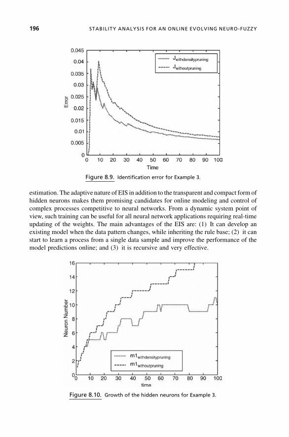
estimation. The adaptive nature of EIS in addition to the transparent and compact form of

hidden neurons makes them promising candidates for online modeling and control of

complex processes competitive to neural networks. From a dynamic system point of

view, such training can be useful for all neural network applications requiring real-time

updating of the weights. The main advantages of the EIS are: (1) It can develop an

existing model when the data pattern changes, while inheriting the rule base; (2) it can

start to learn a process from a single data sample and improve the performance of the

model predictions online; and (3) it is recursive and very effective.




The main contribution of this chapter is the theoretical proof of stability of learning

based on the modified version of the fuzzily weighted recursive least-squares method for

a particular type of evolving fuzzy network (with particular types of consequences).

8.9 ACKNOWLEDGMENTS

We express our gratitude to the editors for inviting us to participate in this project and to

the reviewers for their valuable comments and suggestions, which helped to improve this

research.

8.10 REFERENCES

1. P. P. Angelov, R. Buswell, “Identification of Evolving Fuzzy Rule-Based Models,” IEEE

Trans. on Fuzzy Systems, Vol. 10, No. 5, pp. 667–677, 2002.

2. P. P. Angelov, D. P. Filev, “An approach to Online Identification of Takagi-Sugeno Fuzzy

Models,” IEEE Trans. on Systems, Man and Cybernetics, Vol. 32, No. 1, pp. 484–498, 2004.

3. P. P. Angelov, D. P. Filev, “Simpl_eTS: A Simplified Method for Learning Evolving Takagi-

Sugeno Fuzzy Models.” Int. Con. on Fuzzy Systems, 2005, pp. 1068–1072.

4. M. F. Azem, M. Hanmandlu, N. Ahmad, “Structure identification of Generalized Adaptive

Neuro-Fuzzy Inference Systems,” IEEETrans. onFuzzy Systems, Vol. 11,No. 6, pp. 666–681,

2003.

5. J. C. Bezdek,“Fuzzy Mathematics in Pattern Classification,” PhD thesis, Applied Math.

Center, Cornell University, Ithaca, 1973.

6. E. G. P. Box, G. M. Jenkins, Time Series Analysis, Forecasting and Control. San Francisco:

Holden Day, 1976.

7. M.Brown,C. J.Harris,AdaptiveModeling andControl. NewYork:Macmillan, Prentice-Hall,

1994.

8. J. B. D. Cabrera, K. S. Narendra, “Issues in the Application of Neural Networks for Tracking

Based on Inverse Control,” IEEE Transactions on Automatic Control, Vol. 44, No. 11, pp.

2007–2027, November 1999.

9. S. L. Chiu, “Fuzzy Model Identification Based on Cluster Estimation,” Journal of Intelligent

and Fuzzy Systems, Vol. 2, No. 3, 1994.

10. G. Cybenco, “Approximation by Superposition of Sigmoidal Activation Function,” Math.

Control Sig. System, Vol. 2, pp. 303–314, 1989.

11. B. Egardt, “Stability of Adaptive Controllers,” Springer-Verlag Berlin, Lecture Notes in

Control and Information Sciences, Vol. 20, 1979.

12. G. C. Goodwin, K. Sang Sin, Adaptive Filtering Prediction and Control. Englewood Cliffis,

NJ: Prentice Hall, 1984.

13. J. W. Haefner, Modeling Biological Systems: Principles and Applications. New York:

Springer, 2005, ISBN-10: 0-387-25012-3 (E).

14. D.Hassibi, D.G. Stork,“SecondOrderDerivatives forNetworkPruning,”Advances inNeural

Information Processing, Los Altos, CA, Vol. 5, pp. 164-171, 1993.

15. S. Haykin, Neural Networks. A Comprehensive Foundation. New York: Macmillan, 1994.

REFERENCES 197

16. J. R. Hilera, V. J. Martines, Redes Neuronales Artificiales, Fundamentos, Modelos y

Aplicaciones. Addison-Wesley Iberoamericana, 1995.

17. P. A. Ioannou, J. Sun, Robust Adaptive Control. Upper Saddle River: NJ: Prentice-Hall, 1996.

18. J. S. R. Jang, “AFNFIS: Adaptive-Network-Based Fuzzy Inference System,” IEEE Trans. on

Systems, Man and Cybernetics, Vol. 23, pp. 665–685, 1993.

19. J. S. R. Jang, C. T. Sun, E.Mizutani,Neuro-Fuzzy and Soft Computing. Englewood Cliffs, NJ:

Prentice-Hall, 1996.

20. C. F. Juang, C.T. Lin, “An On-line Self-Constructing Neural Fuzzy Inference Network and Its

Applications,” IEEE Trans. on Fuzzy Systems, Vol. 6, No. 1, pp. 12–32, 1998.

21. C. F. Juang, C.T. Lin, “A Recurrent Self-Organizing Fuzzy Inference Network,” IEEE Trans.

on Neural Networks, Vol. 10, No. 4, pp. 828–845, 1999.

22. C. F. Juang, “A TSK-Type Recurrent Fuzzy Network for Dynamic Systems Processing by

Neural Network and Genetic Algorithms,” IEEE Trans. on Fuzzy Systems, Vol. 10, No. 2, pp.

155–169, 2002.

23. N. K. Kasabov, “Evolving Fuzzy Neural Networks for Supervised/Unsupervised Online

Knowledge-Based Learning,” IEEE Trans. on Systems, Man and Cybernetics, Vol. 31, No. 6,

pp. 902–918, 2001.

24. N. K. Kasabov, Q. Song, “DENFIS: Dynamic Evolving Neural-Fuzzy Inference System and

Its Application for Time-Series Prediction,” IEEETrans. on Fuzzy Systems, Vol. 10, No. 2, pp.

144–154, 2002.

25. K. Kim, E. J. Whang, C.-W. Park, E. Kim, M. Park, A TSK Fuzzy Inference Algorithm for

Online Identification, Berlin, Heidelberg: Springer-Verlag, 2005, pp. 179–188.

26. E. B. Kosmatopoulos, M.M. Polycarpou, M.A. Christodoulou, P.A. Ioannou, “High-order

Neural Network Structures for Identification of Dynamic Systems,” IEEE Trans. on Neural

Networks, Vol. 6, No. 2, pp. 422–431, 1995.

27. G. Leng, T. M. McGinnity, G. Prasad, “An Approach for On-line Extraction of Fuzzy Rules

Using a Self-Organizing Fuzzy Neural Network,” Fuzzy Sets and Systems, Vol. 150, pp.

211–243, 2005.

28. C. T. Lin,Neural Fuzzy Control Systems with Structure and Parameter Learning. NewYork:

World Scientific, 1994.

29. K. S. Narendra, K. Parthasarathy, “Identification and Control of Dynamic Systems Using

Neural Networks,” IEEE Trans. Neural Networks, Vol. 1, No. 1, pp. 4–27, 1990.

30. A. G. Parlos, S. K. Menon, A. F. Atiya, “An Algorithm Approach to Adaptive State Filtering

Using Recurrent Neural Network,” IEEE Trans. Neural Networks, Vol. 12, No. 6, pp.

1411.1432, 2001.

31. J. Platt, “A Resource-Allocating Network for Function Interpolation,” Neural Computation,

Vol. 3, No. 2, pp. 213–225, 1991.

32. I. Rivals, L. Personnaz, “Neural Network Construction and Selection in NonlinearModeling,”

IEEE Trans. on Neural Networks, Vol. 14, No. 4, pp. 804–820, 2003.

33. J. J. Rubio,W.Yu, “ANewDiscrete-Time Sliding-Mode Control with Time-VaryingGain and

Neural Identification,” Int. J. Control, Vol. 79, No. 4, pp. 338–348, April 2006.

34. J. J. Rubio, W. Yu, “Nonlinear System Identification with Recurrent Neural Networks and

Dead-Zone Kalman Filter Algorithm,” Neurocomputing, Vol. 70, pp. 2460–2466, 2007.

35. J. J. Rubio, W. Yu, “Dead-Zone Kalman Filter Algorithm for Recurrent Neural Networks.”

44th IEEE Conf. on Decision and Control, Spain, 2005, pp. 2562–2567.


36. P. S. Sastry, G. Santharam, K. P. Unnikrishnan, “Memory Neural Networks for Identification

and Control of Dynamic Systems,” IEEE Trans. Neural Networks, Vol. 5, pp. 306–319, 1994.

37. S. G. Tzafestas, K. C. Zikidis, “On-Line Neuro-Fuzzy ART-Based Structure and Parameter

Learning TSK Model,” IEEE Trans. on Systems, Man and Cybernetics, Vol. 31, No. 5, pp.

797–803, 2001.

38. L. X. Wang, A Course in Fuzzy Systems and Control. Englewood Cliffs, NJ: Prentice-Hall,

1997.

39. S. Wu, M. J. Er, “Dynamic Fuzzy Neural Networks: A Novel Approach to Function

Approximation,” IEEE Trans. on Systems, Man and Cybernetics—Part B, Vol. 30, pp.

358–364, 2000.

40. S. Wu, M. J. Er, “A Fast Approach for Automatic Generation of Fuzzy Rules by Generalized

Dynamic FuzzyNeural Networks,” IEEE Trans. on Fuzzy Systems, Vol. 9, pp. 578–594, 2001.

41. R. R. Yager, D. P. Filev, “Learning of Fuzzy Rules byMountain Clustering.” Proc. SPIE Conf.

on Application of Fuzzy Logic Technology, Boston, 1993, pp. 246–254.

42. W. Yu, X. Li, “Fuzzy Identification Using Fuzzy Neural Networks with Stable Learning

Algorithms,” IEEE Trans. on Fuzzy Systems, Vol. 12, No. 3, pp. 411–420, 2004.

REFERENCES 199

9ONLINE IDENTIFICATION OFSELF-ORGANIZING FUZZYNEURAL NETWORKS FOR

MODELING TIME-VARYINGCOMPLEX SYSTEMS

G. Prasad, G. Leng, T.M. McGinnity, D. Coyle

Abstract: Fuzzy neural networks are hybrid systems that combine the theories of fuzzy

logic and neural networks. By incorporating in these hybrid systems the ability to self-

organize their network structure, self-organizing fuzzy neural networks (SOFNNs) are

created. The SOFNNs have enhanced ability to identify adaptive models, mainly for

representing nonlinear and time-varying complex systems, where little or insufficient

expert knowledge is available to describe the underlying behavior. Problems that arise

in these systems are large dimensions, time-varying characteristics, large amounts of

data, and noisy measurements, as well as the need for an interpretation of the resulting

model.

This chapter presents an algorithm for online identification of a self-organizing

fuzzy neural network. The SOFNN provides a singleton or Takagi-Sugeno (TS)-type

fuzzy model. It therefore facilitates extracting fuzzy rules from the training data. The

algorithm is formulated to guarantee the convergence of both the estimation error and

the linear network parameters. It generates a fuzzy neural model with high accuracy

and compact structure. Superior performance of the algorithm is demonstrated through

its applications for function approximation, system identification, and time-series

prediction in both industrial and biological systems.


and Nikola Kasabov


9.1 INTRODUCTION

In order to effectively handle the complexity and dynamics of real-world problems, there

is often the need to model online nonlinear and time-varying complex systems. Such a

need arises in both industrial and biological systems, for example, models for market

forecasts, optimal manufacturing control, and administering anesthesia optimally.

The complexity of modeling these systems is exacerbated due to the fact that there

is often very little or insufficient expert knowledge available to describe the underlying

behavior. Additional common problems that arise in these systems are large dimensions,

large amounts of data, and noisy measurements. In such cases, it is thus an obvious

requirement that an appropriate modeling algorithm should have a much higher level of

autonomy in themodeling process as well as being capable of providing an interpretation

of the resulting model. In order to meet these stringent modeling requirements, an

algorithm developed using a hybrid intelligent systems approach is reported in this

chapter. The algorithm is basically a fuzzy neural network (FNN) identification

procedure, in which fuzzy techniques are used to enhance certain aspects of the neural

network’s learning and adaptation performance. FNNs are usually represented as

multilayer feedforward networks and are used to learn fuzzy membership functions

and explain the rules that are used to make decisions. A good review about FNNs can be

found in Buckley and Hayashi (1994) and Nauck (1997). Some authors make a

distinction between FNNs and neuro-fuzzy systems. However, no differentiation is

made in this chapter. The algorithmwe are discussing is based on a self-organizing fuzzy

neural network (SOFNN) approach, in which the FNN possesses an ability to self-

organize its structure along with associated premise parameters. A type of recursive

least-squares (RLS) algorithm (Astrom & Wittenmark, 1995) forms an integral part of

the approach. This is used to identify consequent parameters of a singleton or Takagi-

Sugeno (TS)-type (Takagi & Sugeno, 1985) fuzzy model. Thus, the main purpose of the

SOFNN approach here is to devise a hybrid fuzzy neural network architecture to create

self-adaptive fuzzy rules for online identification of a singleton or TS-type fuzzy model

of a nonlinear time-varying complex system. The associated algorithm therefore aims to

create a self-organizing neural network that is designed to approximate a fuzzy algorithm

or a process of fuzzy inference through the structure of neural networks and thus create a

more interpretable hybrid neural network model making effective use of the superior

learning ability of neural networks and easy interpretability of fuzzy systems. The twin

main issues associated with the identification of a singleton or TS-type fuzzy model are:

(1) structure identification, which involves partitioning the input–output space and thus

identifying the number of fuzzy rules for the desired performance, and (2) parameter

estimation, which includes identifying parameters of premises and consequences.

With sufficient good-quality training data, there are several supervised training ap-

proaches (Mitra & Hayashi, 2000; Wang & Lee, 2001) proposed in the literature for an

adaptive fuzzy neural model identification. The main difference lies in the method

adopted for the partitioning of input–output space for the structure identification. As

suggested in Wang and Lee (2001), the methods proposed in the literature can be placed

into two broad categories: (1) the static adaptation method, where the number of

input–output partitions are fixed, while their corresponding fuzzy rule configurations are

202 ONLINE IDENTIFICATION OF SELF-ORGANIZING FUZZY NEURAL

adapted through optimization to obtain the desired performance, and (2) the dynamic

adaptation method, where both the number of input–output space partitions and their

corresponding fuzzy rule configurations are simultaneously and concurrently adapted.

The main focus of the SOFNN algorithm is the design of an approach for dynamic

adaptation of the structure of the hybrid network, so that the underlying behavior of

a nonlinear time-varying complex system could be captured in a model that is more

accurate, compact, and interpretable.

For similar performance, the number of fuzzy partitions, and thereby fuzzy rules, can be

greatly reduced by cluster-based partitioning of the input–output space (Zadeh, 1994).

Therefore, for identifying a more compact structure, input–output space partitioning

based on the traditional clustering approaches, such as hard c-means (HCM) and fuzzy

c-means (FCM) (Gonzalez et al., 2002; Klawonn & Keller, 1998; Wang & Lee, 2001),

has been proposed. The number of partitions, however, needs to be fixed by a priori

expert knowledge in these approaches. The final configuration of the clusters and the

corresponding fuzzy rule parameters are obtained by a nonlinear optimization. However,

there is no guarantee of convergence to an optimal solution, as the final solution greatly

relies on the selection of initial locations of cluster centers. Also, it is difficult and time

consuming tovisualize the optimal number of partitions required formodeling a complex

system, particularly if the underlying structural behavior of the system is time-varying

and inadequately known.

Under the dynamic adaptationmethod, the trainingmay start with a single fuzzy rule

or neuron or none at all (Er&Wu, 2002; Kasabov&Song, 2002; Rizzi et al., 2002;Wang

& Lee, 2001; Wu & Er, 2000; Wu et al., 2001). During training, the network structure

grows and concurrently the parameters of antecedents and consequents are adapted to

obtain the desired modeling accuracy.

A constructive approach for creating on ANFIS-like network is proposed in

(Mascioli & Martinelli, 1998; Mascioli et al., 2000; Rizzi et al., 2002) based on

Simpson’s min-max technique (Simpson, 1992;1993). The input space is partitioned

by constructing hyperboxes using the min-max procedure. The hyperbox-based frame-

work facilitates application of different types of fuzzy membership functions. To

decrease the complexity of the network, a pruning method, called pruning adaptive

resolution classifier (PARC), is developed in Rizzi et al. (2002). This consists of deleting

some negligible hyperboxes and a fusion procedure to make actual coverage complete.

This constructive approach is, however, basically developed for batch learning to create a

structure-adaptive network with a significantly higher degree of automation.

A dynamic fuzzy neural network (DFNN) architecture reported inWu and Er (2000)

and Er and Wu (2002) is another notably relevant work. It makes use of a hierarchical

learning approach and an orthogonal least-squares-based pruning technique (Chen

et al., 1991). In the DFNN architecture, fuzzy rules are represented by radial basis

function (RBF) neurons in the first hidden layer. However, the representation is restrictive

in the sense that widths of the membership functions belonging to various inputs that

create anRBFneuron of theDFNNhave the samevalue.An enhanced version ofDFNN is

GDFNN (Wu et al., 2001). It introduces width vectors in RBF neurons, so that the

Gaussian membership functions within a neuron can be assigned appropriate widths

separately. The GDFNN also attempts to provide explanations for selecting the values of

INTRODUCTION 203

width parameter of the Gaussian fuzzy membership functions based on the concept of e-completeness (Wang, 1992). However, the hierarchical learning approach proposed for

training GDFNN is dependent on the total number of training data patterns. This implies

that theGDFNNapproach is primarily designed for batch training using a fixed number of

training data patterns.

The dynamic evolving neuro-fuzzy system (DENFIS) is another notable approach

(Kasabov & Song, 2002) that employs a dynamic adaptation method and can be applied

in online TS-type model identification. The input space partitioning in DENFIS is

accomplished online using an evolving clustering method (ECM) that creates new

clusters as newdata vectors arrive, based on a distance threshold. The fuzzy inference and

thereby the consequent parameters are estimated based on only the nearestm fuzzy rules.

Although this approach implements the concept of local learning by limiting the learning

in the region nearest to the current data vector, it has no provision to ensure that network

size remains compact while ensuring higher generalization accuracy.

SOFNN is in the same category of approaches as eTS (Angelov and Filev, 2004).

In order to model a time-varying nonlinear system, a truly online training algorithm is

required so that the desired accuracy as well as network size can be obtained. Ensuring

convergence of the network parameters and the estimation error is also essential for

an online training algorithm. Based on the dynamic adaptation method, this chapter

presents an algorithm for creating a self-organizing fuzzy neural network that identifies

a singleton or TS-type fuzzy model online. A modified recursive least-squares (RLS)

algorithm derived to guarantee the convergence of the estimation error and the linear

network parameters is used for estimating consequent parameters. For structure

learning, the algorithm makes use of a procedure to decide how to create a new

ellipsoidal basis function (EBF) neuron with a center vector and a width vector. The

EBF neuron represents a fuzzy rule formed by AND logic (or T-norm) operating on

Gaussian fuzzy membership functions. The elements of center vector and width vector

of the EBF neurons are the centers and widths of the Gaussian membership functions.

The structure learning approach consists of a combination of system error and firing

strength–based criteria for adding newEBF neurons using the concepts from statistical

theory and the e-completeness of fuzzy rules (Lee, 1990). This ensures that the

membership functions have the capability to cover more data. The SOFNN approach

uses a pruning method based on the optimal brain surgeon (OBS) approach (Hassibi &

Stork, 1993; Leung et al., 2001). This method is computationally very efficient for

online implementation, as it does not involve any significant additional computation

because it makes direct use of the Hermitian matrix obtained as a part of the RLS

algorithm. These two features of adding and pruning neurons automatically enable the

SOFNN to have an adaptive structure to model nonlinear and time-varying systems

online. The structure learning and parameter learning methods are very simple and

more efficient and yield a fuzzy neural model with high accuracy and compact

structure.

In the next section, the architecture of the SOFNN is described. The structure

learning of the SOFNN that presents the approach of adding and pruning neurons is

organized in Section 9.2. It also describes the modified RLS algorithm and the analysis

of the properties of this algorithm for the parameter learning. Typical applications and


a performance evaluation of the SOFNN algorithm are discussed in Section 9.3. Finally,

conclusions are summarized in Section 9.4.

9.2 ALGORITHMIC DETAILS

9.2.1 Architecture of the SOFNN

The architecture of the self-organizing fuzzy neural network is a five-layer fuzzy neural

network, shown in Figure 9.1. The five layers are the input layer, the ellipsoidal basis

function (EBF) layer, the normalized layer, the weighted layer, and the output layer.

Some of the interconnections are shown by dotted lines. This is to indicate that the

SOFNN has the ability to self-organize its own neurons in the learning process for

implementing singleton or Takagi-Sugeno (TS)-fuzzy models.

In the EBF layer, each neuron is a T-norm of Gaussian fuzzy membership functions

belonging to the inputs of the network. Every membership function (MF) thus has its

own distinct center and width, which means every neuron has both a center vector and

awidthvector and thedimensionsof thesevectorsare the sameas thedimensionof the input

vector. Figure 9.2 illustrates the internal structure of the jth neuron, where

x ¼ x1 x2 . . . . . . xr½ � is the input vector, cj ¼ c1j c2j . . . . . . crj½ � is the

vector of centers in the jth EBF neuron, and sj ¼ s1j s2j . . . . . . srj½ � is the

vector of widths in the jth neuron. Here, multi-input, single-output (MISO)

systems are considered. However, all results could also be applied to multi-input, multi-

output (MIMO) systems. A layerwise mathematical description of the network follows.

Layer 1 is the input layer. Each neuron in this layer represents an input variable,

xi, i ¼ 1; 2; . . . ; r.Layer 2 is the EBF layer. Each neuron in this layer represents an if-part (or premise)

of a fuzzy rule. The outputs of EBF neurons are computed by products of the grades of

Figure 9.1. Self-organizing fuzzy neural network.

ALGORITHMIC DETAILS 205

MFs. Each MF is in the form of a Gaussian function,

mij ¼ exp � ðxi � cijÞ22s2

ij

" #

i ¼ 1; 2; . . . ; r; j ¼ 1; 2; . . . ; u

ð9:1Þ

where mij is the ith membership function in the jth neuron; cij is the center of the ith

membership function in the jth neuron; sij is the width of the ith membership function

in the jth neuron; r is the number of input variables; and u is the number of neurons.

For the jth neuron, the output is

fj ¼ exp �Xri¼1

ðxi � cijÞ22s2

ij

" #

j ¼ 1; 2; . . . ; u

ð9:2Þ

Layer 3 is the normalized layer. The number of neurons in this layer is equal to that

of layer 2. The output of the jth neuron in this layer is

cj ¼fjXu

k¼1fk

¼exp �

Xri¼1

ðxi� cijÞ22s2

ij

" #

Xuk¼1

exp �Xri¼1

ðxi � cikÞ22s2

ik

" #j ¼ 1; 2; . . . ; u

ð9:3Þ

Layer 4 is the weighted layer. Each neuron in this layer has two inputs and the

product of these inputs as its output.One of the inputs is the output of the related neuron in

layer 3 and the other is theweighted biasw2j obtained as the dot product of the bias vector

MF1j

(c1j, σ1j)

MF2j

(c2j, σ2j)

MFrj

(crj, σrj)

x1

x2

xr

φj

μ1j

μ2j

μrj

Π

Figure 9.2. Structure of the jth neuron Rj with cj and sj in the EBF layer.


B and the row vector Aj. For the Takagi-Sugeno (TS) model (Takagi & Sugeno, 1985),

the bias is the column vector B ¼ ½1 x1 x2 . . . xr�T. For the singleton fuzzy model,

B ¼ ½1 0 0 � � � 0�T . The dimension of the column vector B is rþ 1. The row vector

Aj ¼ aj0 aj1 aj2 . . . . . . ajr½ � represents the set of parameters corresponding to the

then-part (or consequent) of the fuzzy rule j. The weighted bias w2j is

w2j ¼ Aj �B ¼ aj0þ aj1x1þ � � � þ ajrxr

j ¼ 1; 2; . . . ; uð9:4Þ

This is thus the then-part (or consequent) of the jth fuzzy rule of the fuzzymodel. The

output of each neuron is fj ¼ w2jcj .

Layer 5 is the output layer. Each neuron in this layer represents an output variable

as the summation of incoming signals from layer 4. The output of a neuron in layer 5 is

yðxÞ ¼Xuj¼1

fj

¼

Xuj¼1

w2j exp �Xri¼1

ðxi � cijÞ22s2

ij

" #

Xuk¼1

exp �Xri¼1

ðxi � cikÞ22s2

ik

" #ð9:5Þ

where y is the value of an output variable.

Suppose uEBF neurons are generated from the n training patterns of the input vector

xt and the corresponding desired output dtðt ¼ 1; 2; . . . ; nÞ. Rewrite the output of the

network as

Y ¼W2Y ð9:6Þ

where, for the TS model,

Y ¼ y1 y2 . . . yn½ � ð9:7Þ

W2 ¼ a10 a11 . . . a1r . . . au0 au1 . . . aur½ � ð9:8Þ

Y ¼

c11 . . . c1n

c11x11 . . . c1nx1n

..

. ... ..

.

c11xr1 . . . c1nxrn

..

. ... ..

.

cu1 . . . cun

cu1x11 . . . cunx1n

..

. ... ..

.

cu1xr1 . . . cunxrn

26666666666666664

37777777777777775

ð9:9Þ


whereW2 is the parametermatrix, andcjt is the output of the jth neuron in the normalized

layer when the tth training pattern enters the network.

9.2.2 The SOFNN Learning Algorithm

The learning process of the SOFNN includes the structure learning and the parameter

learning. The structure learning attempts to achieve an economical network size with

a self-organizing approach. As a result of this, neurons in the EBF layer are augmented

or pruned dynamically in the learning process. The parameter learning makes the

network converge quickly through an online recursive least-squares algorithm.

9.2.2.1 Adding aNeuron. There are two criteria to judgewhether to generate an

EBF neuron. One is the system error criterion, and the other is the coverage or the if-part

criterion. The error criterion considers the generalization performance of the overall

network. The if-part criterion evaluates whether existing fuzzy rules or EBF neurons can

cover and cluster the input vector suitably.

The Error Criterion: Consider the nth observation ðxn; dnÞ, where xn is the input

vector and dn is the desired output. The output of the network with the current structure

is yn. The system error eðnÞ is defined as

eðnÞj j ¼ dn� ynj j ð9:10Þ

If

eðnÞj j > d ð9:11Þ

where d is the predefined error tolerance, a new EBF neuron should be considered either

for addition to the structure or to modify the widths of some membership functions.

TheCoverageCriterion:EveryEBFneuron in the EBF layer represents an if-part ofa fuzzy rule. For the nth observation ðxn; dnÞ with r as the dimension of input vector, the

firing strength or the output of each EBF neuron is

fj ¼ exp �Xri¼1

ðxin� cijÞ22s2

ij

" #j ¼ 1; 2; . . . ; u ð9:12Þ

The input vector xn would be assumed to have been appropriately clustered by

existing fuzzy rules or EBF neurons if the firing strength of at least one neuron is greater

than 0.1354. This condition would ensure that no individual input can have a fuzzy

membership grade less than 0.1354, and thus the e-completeness of fuzzy rules

(Lee, 1990), with e ¼ 0:1354, would be satisfied. It is also to be noted that for a Gaussianmembership function MFðcij;sijÞ the membership grade is 0.1354 for the inputs at

cij � 2sij . Assuming a normal input data distribution, 95% of input data belonging to

this membership function will lie within the input range ½cij � 2sij ; cij þ 2sij�.


Now define

fðnÞ ¼ maxj¼1......u

ðfjÞ ð9:13Þ

If fðnÞ < 0:1354, it means no neuron in this structure can cluster this input vector. So,

the width should be modified to cover the input vector suitably or a new EBF neuron

should be considered for adding into the structure. Keeping the neuron output threshold

constant, the capability of membership functions for covering input vectors may be

increased by enlarging the widths of membership functions.

When the first training pattern ðx1; d1Þ enters the network, the structure of the firstneuron is defined as

c1 ¼ xT1 ð9:14Þ

s1 ¼ s0 s0 � � � s0½ �T ð9:15Þ

where c1 is the center vector whose dimension is r 1, s1 is the width vector whose

dimension is r 1, and s0 is a predefined initial width.

For the nth training pattern, the following scenarios are possible:

1. eðnÞj j � d and fðnÞ � 0:1354: This means that the network has good general-

ization and some neurons can cluster this input vector. The fuzzy neural network

can thus accommodate the observation. Either nothing should be done or only

the parameters should be adjusted.

2. eðnÞj j � d and fðnÞ < 0:1354: In this case, the network has good generalization,but no neuron can cluster this input vector. To ensure the e-completeness of

fuzzy rules, the widths of this EBF neuron should be enlarged to make its output

match the threshold 0:1354. So, the width of the membership function that has

the least value in this neuron should be enlarged to cover the input vector suitably

using (9.21), described later.

3. eðnÞj j > d and fðnÞ � 0:1354: This means that the network has poor general-

ization performance but a neuron can cluster the current input vector. Thus,

despite proper coverage of the current input by the existing neurons, the

generalizationperformanceof thenetwork ispoor.AnewEBFneuron is therefore

required to be added to the current structure to improve the performance.

Suppose the kth new neuron is to be added to the structure. For every neuron in

the EBF layer except the kth new neuron, find the minimum distance vector,

Distk ¼

dist1nðhm1Þdist2nðhm2Þ

..

.

distrnðhmrÞ

26664

37775 ¼

minj¼1; �� ;k� 1

ð x1n� c1j Þ

minj¼1; �� ;k� 1

ð x2n� c2j Þ...

minj¼1; �� ;k� 1

ð xrn� crj Þ

266666664

377777775

ð9:16Þ


where distinðhmiÞ is the distance between the ith input of the nth observation

xn ¼ ½x1n x2n . . . . . . xrn� and the center of the hmith membership function

in the mith neuron. The center cihmiof the hmith membership function is the

nearest center from xin. Here i ¼ 1; 2; . . . . . . r. Let the center vector ck and the

width vector sk of the kth new neuron be

ck ¼ c1k c2k . . . crk½ �T ð9:17Þand

sk ¼ s1k s2k . . . srk½ �T ð9:18Þ

If distinðhmiÞ � kdðiÞ, where kdðiÞ is a predefined distance threshold of the ith

input, i ¼ 1; 2; . . . r, then

cik ¼ cihmi

sik ¼ sihmi

ð9:19Þ

and if distinðhmiÞ > kdðiÞ, then

cik ¼ xinsik ¼ distinðhmiÞ ð9:20Þ

The parameters of the current network should be updated tominimize the system

error eðnÞ since there is a new neuron added in this situation.

4. eðnÞj j > d and fðnÞ < 0:1354: This shows that the network has poor general-

ization and no neurons can cluster this input vector. The strategy for this case is to

try improving the entire performance of the current network by enlarging some of

the widths to cover the current input vector. Suppose fðnÞ is the output of the jthEBF neuron. Thewidth of the ith membership function that has the least value in

this neuron should be enlarged to cover the input vector suitably:

snewij ¼ kss

oldij ð9:21Þ

whereks is a predefined constant that is larger than 1. For simulations in this chapter,

ks ¼ 1:12. The width enlargement process is continued until fðnÞ � 0:1354. If thenetwork still has bad generalization, that is, eðnÞj j > d, the old widths are main-

tained and a new EBF neuron is added to the structure using the same procedure as

described in the scenario 3. The parameters of the new network also should be

updated.

9.2.2.2 The Linear Parameter Learning Method. The SOFNN model could

be rewritten as a special case of a linear regression model

dðtÞ ¼XMi¼1

piðtÞqi þ eðtÞ ð9:22Þ


where dðtÞ is the desired output; piðtÞ is the ith regressor, which is a fixed function of

input vector xt ¼ x1t x2t . . . xrt �½ , that is, piðtÞ ¼ piðxtÞ; qi is the ith linear

parameter; eðtÞ is the error signal; and Mis the dimension of the parameters, here,

M ¼ u ðrþ 1Þ.Using (9.6) through (9.9), (9.22) can be written in matrix form at time t ¼ n as

DðnÞ ¼ PðnÞQðnÞþEðnÞ ð9:23Þ

where,DðnÞ¼ dð1Þ dð2Þ . . . dðnÞ½ �T 2Rn;PðnÞ ¼ YT ¼ ½pTð1Þ pTð2Þ . . .pTðnÞ�T 2RnM , and pTðiÞ ¼ p1ðiÞ p2ðiÞ . . . pMðiÞ½ �, 1 � i � n; QðnÞ ¼WT

2 ¼q1 q2 . . . qM½ �T 2 RM; and EðnÞ ¼ eð1Þ eð2Þ . . . eðnÞ½ �T 2 Rn.

Using the linear least-squares method, the parameter of the regression model is

given by

QðtÞ ¼ ½PTðtÞPðtÞ�� 1PTðtÞDðtÞ ð9:24Þ

Based on the RLS algorithm (Astrom & Wittenmark, 1995) at time t, an online

weight learning algorithm is developed for the parameter learning. Define an M M

Hermitian matrix Q as

QðtÞ ¼ ½PTðtÞPðtÞ�� 1 ð9:25Þ

Using the matrixQ, the final update equations of the standard RLS algorithm can be

written as

LðtÞ ¼ QðtÞpðtÞ ¼ Qðt� 1ÞpðtÞ½1þ pTðtÞQðt� 1ÞpðtÞ�� 1 ð9:26Þ

QðtÞ ¼ ½I�LðtÞpTðtÞ�Qðt� 1Þ ð9:27Þ

QðtÞ ¼ Qðt� 1ÞþLðtÞ½dðtÞ� pTðtÞQðt� 1Þ� ð9:28Þ

In order to ensure convergence, a variation of the above standard recursive least-

squares algorithm is used. At time t, when the estimation error eðtÞj j is less than the

approximation error eðtÞj j, the parameters of the network are not adjusted and the

structure is also not modified. Thus, the online learning algorithm is modified to:

LðtÞ ¼ QðtÞpðtÞ ¼ Qðt� 1ÞpðtÞ½1þ pTðtÞQðt� 1ÞpðtÞ�� 1 ð9:29Þ

QðtÞ ¼ ½I�aLðtÞpTðtÞ�Qðt� 1Þ ð9:30Þ

QðtÞ ¼ Qðt� 1ÞþaLðtÞ½dðtÞ� pTðtÞQðt� 1Þ� ð9:31Þ

a ¼ 1; eðtÞj j � eðtÞj j0; eðtÞj j < eðtÞj j

�ð9:32Þ

where eðtÞ ¼ ½dðtÞ� pTðtÞQðt� 1Þ�; eðtÞ ¼ ½dðtÞ� pTðtÞQðtÞ�.


This modification ensures that the above modified algorithm guarantees an asymp-

totic convergence of the estimation error to zero and the convergence of the parameter

to finite values. The proof of the convergence is detailed in Leng et al. (2004).

9.2.2.3 Pruning a Neuron. In the learning process, the network reaches a local

minimum in error. The cost function is defined as the squared error, EðQ; tÞ ¼12

Pti¼1 ½dðiÞ� pTðiÞQ�2. At time t, using the functional Taylor series of the error

with respect to parameters Q, it can be shown that (Gang et al., 2004):

DEðQ; tÞ � 1

2DQTHDQ ð9:33Þ

where

H ¼ @2EðQ; tÞ@Q2

¼Xti¼1

pðiÞpTðiÞ ¼ PTðtÞPðtÞ ¼ Q� 1ðt� 1Þþ pðtÞpTðtÞ ¼ Q� 1ðtÞ

ð9:34ÞDeleting a neuron is equivalent to setting the values of the related parameters to zero.

The smaller the value of the change in the squared error, the less important is the neuron.

Based on these twin concepts, the pruning method is designed using the following steps:

1. Calculate the training root mean squared error Ermse at time t.

2. Define the tolerance limit for the root mean squared error as lErmse, where l is

a predefined value and 0 < l < 1. For simulations in this chapter, l ¼ 0:8.

3. Calculate the change of the squared error DE for every neuron. The smaller the

value of DE is, the less important is the neuron.

4. Choose E ¼ maxðlErmse; krmseÞ, where krmse is the expected training root mean

squared error, which is a predefined value.

5. Select the least important neuron, delete this neuron, and then calculate the

training rootmean squared error ðERMSEÞ of this new structure. IfERMSE < E, this

neuron should be deleted. Then do the same thing for the second least important

neuron, and so on. Otherwise, stop and do not delete any more neurons.

9.2.2.4 CombiningMembership Functions andRules. If somemembership

functions are very similar to each other, they can be in the same group and combined into

one new membership function as in Wang (1997). In the SOFNN algorithm, the

membership functions that have the same center are combined into one new

membership function. Consider n membership functions that have the same center csand different widths ss1;ss2; . . . . . . ;ssn. The new membership function is defined with

the center

cnew ¼ cs ð9:35Þ


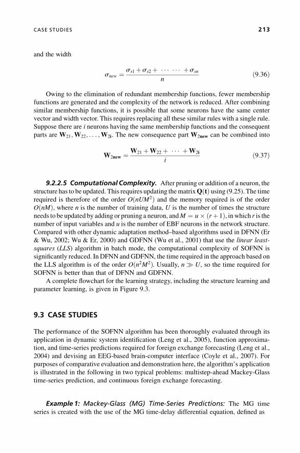
and the width

snew ¼ ss1þss2þ � � � � � � þssn

nð9:36Þ

Owing to the elimination of redundant membership functions, fewer membership

functions are generated and the complexity of the network is reduced. After combining

similar membership functions, it is possible that some neurons have the same center

vector and width vector. This requires replacing all these similar rules with a single rule.

Suppose there are i neurons having the same membership functions and the consequent

parts are W21;W22; . . . ;W2i. The new consequence part W2new can be combined into

W2new ¼W21þW22þ � � � þW2i

ið9:37Þ

9.2.2.5 Computational Complexity. After pruning or addition of a neuron, the

structure has to be updated. This requires updating thematrixQðtÞ using (9.25). The time

required is therefore of the order OðnUM2Þ and the memory required is of the order

OðnMÞ, where n is the number of training data, U is the number of times the structure

needs to be updated by adding or pruning a neuron, andM ¼ u ðrþ 1Þ, inwhich r is thenumber of input variables and u is the number of EBF neurons in the network structure.

Compared with other dynamic adaptation method–based algorithms used in DFNN (Er

& Wu, 2002; Wu & Er, 2000) and GDFNN (Wu et al., 2001) that use the linear least-

squares (LLS) algorithm in batch mode, the computational complexity of SOFNN is

significantly reduced. In DFNN and GDFNN, the time required in the approach based on

the LLS algorithm is of the order Oðn2M2Þ. Usually, n U, so the time required for

SOFNN is better than that of DFNN and GDFNN.

A complete flowchart for the learning strategy, including the structure learning and

parameter learning, is given in Figure 9.3.

9.3 CASE STUDIES

The performance of the SOFNN algorithm has been thoroughly evaluated through its

application in dynamic system identification (Leng et al., 2005), function approxima-

tion, and time-series predictions required for foreign exchange forecasting (Leng et al.,

2004) and devising an EEG-based brain-computer interface (Coyle et al., 2007). For

purposes of comparative evaluation and demonstration here, the algorithm’s application

is illustrated in the following in two typical problems: multistep-ahead Mackey-Glass

time-series prediction, and continuous foreign exchange forecasting.

Example 1: Mackey-Glass (MG) Time-Series Predictions: The MG time

series is created with the use of the MG time-delay differential equation, defined as

CASE STUDIES 213

Feed training data(Xi, di), i = 1,2,…,n

No neuron in thestructure?

Update theparameters (Qi, Θi)Eqs. (9.29)–(9.32)

Initialize the firstneuron (c1, σ1)

Eqs. (9.14), (9.15)

Initialize theparameters (Q1, Θ1)

Eqs. (9.25), (9.24)

Calculate the error andif-part criteria

Eqs. (9.10), (9.13)

|ε(i)| > δ?

φ(i) < 0.1354?

Prune neurons?Eqs. (9.33), (9.34)

Add a new neuron andupdate the structure

Eqs. (9.16)–(9.20), (9.24), (9.25)

i = n+1?

Stop

Prune neurons

Y

N

Y

N

Y

N

Y

N

Y

N

φ(i) < 0.1354?NY

Enlarge the widthEqs. (9.21)

Enlarge the widthEqs. (9.21)

Figure 9.3. Flowchart for the learning strategy.


dx

dt¼ bxðt� tÞ

1þ x10ðt� tÞ � 0:1xðtÞ

b ¼ 0:2; t ¼ 17; xð0Þ ¼ 1:2

ð9:38Þ

To obtain values at integer time points, the fourth-order Runge-Kutta method was

used to find the numerical solution to theMG equation (9.38). Here, we assume that time

step is 0.1. The task is to predict the values from input vectors for any value of the time.

For the purpose of a comparative analysis, we list the performance of existing online

learningmodels neural gas (Fritzke, 1995), RAN (Platt, 1991), andDENFIS (Kasabov&

Song, 2002) applied for the same task and reported in (Kasabov, 2007). Here, the

performance is evaluated in terms of the nondimensional error index (NDEI), which is

defined as the root mean-square error (RMSE) divided by the standard deviation of the

target series.

In order to obtain the multistep-ahead predictive model, 3000 input-target data

between t ¼ 201 and 3200 are used as the training data, and another 500 input-target data

between t ¼ 5001 and 5500 are used as the testing data. The predictionmodel is given by

xðtþ 85Þ ¼ f ðxðtÞ; xðt� 6Þ; xðt� 12Þ; xðt� 18ÞÞ ð9:39Þ

It is thus used to predict the value of the next, 85th step. There are four inputs and one

output. The values of the training parameters are d ¼ 0:15, s0 ¼ 0:1, krmse ¼ 0:05,kdð1Þ ¼ 0:1, kdð2Þ ¼ 0:1, kdð3Þ ¼ 0:1, kdð4Þ ¼ 0:1. The results are shown in Table 9.1and Figures 9.4 to 9.8. One neuron is pruned in the learning process as seen in Figure 9.7.

From Table 9.1, it is clear that the application of SOFNN results in a network of

much smaller size and relatively favorable generalization performance. It is possible to

further improve the generalization performance by selecting more stringent training

parameters. Also, compared to DFNN and GDFNN approaches, the SOFNN provides

favorable performance, when applied in chaotic time-series prediction as discussed in

(Leng et al. 2004).

Example 2: Currency Exchange Rate Prediction: A set of real data is applied

in the investigation for the forecasting problem and to demonstrate the effectiveness of the

proposed algorithm.Thedata represent the daily averaged exchange rates between theUK

pound and the U.S. dollar during the period from January 3, 1986 toMay 31, 2002. There

T A B L E 9.1. Results of Mackey-Glass Time-Series Prediction

Methods

Number of

Neurons/Fuzzy Rules

NDEI for

Testing Data

Neural gas (Fritzke, 1995) 1000 0.062

RAN (Platt, 1991) 113 0.373

DENFIS (Kasabov & Song, 2002) 58 0.276

DENFIS (Kasabov & Song, 2002) 883 0.042

SOFNN 12 0.2159

CASE STUDIES 215

are 4281 observations. These data are divided into two sets. The first 3000 data are the

training data and other data are the testing data. In the N-step-ahead predictive model

yðtþNÞ ¼ f ðyðtÞ; yðt� tÞ; . . . ; yðt�ðn� 1ÞtÞÞ ð9:40Þ

defining N ¼ 6, t ¼ 1, and n ¼ 6, the prediction model is given by

yðtþ 6Þ ¼ f ðyðtÞ; yðt� 1Þ; yðt� 2Þ; yðt� 3Þ; yðt� 4Þ; yðt� 5ÞÞ ð9:41Þ

This model thus has six inputs and one output and is used to predict the value of

the next, 6th step. The values of the training parameters are d ¼ 0:05, s0 ¼ 0:4,

Figure 9.5. RMSE during training.

Figure 9.4. Training result (– desired output, � network output).


krmse ¼ 0:01, kdð1Þ ¼ 0:2, kdð2Þ ¼ 0:2, kdð3Þ ¼ 0:2, kdð4Þ ¼ 0:2, kdð5Þ ¼ 0:2,kdð5Þ ¼ 0:2, kdð6Þ ¼ 0:2. The results are shown in Figures 9.9 to 9.14. The fuzzy rulesextracted during the training are listed in the appendix of the end of the chapter.

Thus, a 25-EBF-neuron network is generated. The RMSE of training data is 0.0266.

The RMSE of testing data is 0.0183. Figure 9.15 shows a frequency distribution of

prediction errors for 6-step-ahead prediction. This histogram gives a Gaussian distri-

bution. The mean is �0.0044 and the standard deviation is 0.0177. As the average of

errors is near 0 and the spread of errors is small, this figure shows that the obtained

network is a valid model. The coefficient of correlation for the testing target and testing

output is 0.9824.

Figure 9.7. Growth of neurons.

Figure 9.6. Errors during training.

CASE STUDIES 217

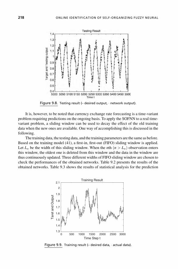
It is, however, to be noted that currency exchange rate forecasting is a time-variant

problem requiring predictions on the ongoing basis. To apply the SOFNN to a real time-

variant problem, a sliding window can be used to decay the effect of the old training

data when the new ones are available. One way of accomplishing this is discussed in the

following.

The training data, the testing data, and the training parameters are the same as before.

Based on the training model (41), a first-in, first-out (FIFO) sliding window is applied.

Let Lw be the width of this sliding window. When the nth ðn > LwÞ observation enters

this window, the oldest one is deleted from this window and the data in the window are

thus continuously updated. Three different widths of FIFO sliding window are chosen to

check the performances of the obtained networks. Table 9.2 presents the results of the

obtained networks. Table 9.3 shows the results of statistical analysis for the prediction

0 500 1000 1500 2000 2500 30001.3

1.4

1.5

1.6

1.7

1.8

1.9

2

2.1Training Result

Time Step t

Tar

et a

nd O

utpu

t

Figure 9.9. Training result (– desired data, � actual data).

Figure 9.8. Testing result (– desired output, � network output).


errors. The distribution of the testing errors for the sliding windowwhose width is 120 is

depicted in Figure 9.16.

Considering the complexity and statistical analysis of the obtained networks using

the three slidingwindows, the sliding windowwhosewidth is 120 has the best coefficient

of correlation and yields a smaller structure. This size of thewidth for the slidingwindow

may thus be a satisfactory choice.

9.4 CONCLUSION

The chapter has discussed an algorithm for creating a self-organizing fuzzy neural

network (SOFNN) that can identify a singleton or TS-type fuzzymodel online. Based on

Figure 9.11. Errors during training.

0 500 1000 1500 2000 2500 30000

0.005

0.01

0.015

0.02

0.025

0.03

0.035RMSE during Training

Time Step t

RM

SE

Figure 9.10. RMSE during training.

CONCLUSION 219

the dynamic adaptation method, both the number of input–output space partitions and

their corresponding fuzzy rule configurations are simultaneously and concurrently

adapted by the SOFNN algorithm. The architecture of the SOFNN consists of ellipsoidal

basis function (EBF) neurons with a center vector and a width vector in the first hidden

layer. The EBF neuron represents the premise part of a fuzzy rule formed by AND logic

(or T-norm) operating on Gaussian fuzzy membership functions. The elements of center

vector and width vector of the EBF neuron are the centers and widths of the Gaussian

membership functions. The structure learning approach combines the system error

criterion and firing strength-based coverage criterion for adding new EBF neurons using

Figure 9.13. Testing result (– desired data, � actual data).

Figure 9.12. Growth of neurons.


concepts from statistical theory and the e-completeness of fuzzy rules. The algorithm

includes a pruning method that is based on the optimal brain surgeon (OBS) approach.

This method is computationally very efficient for online implementation, as it does not

involve any significant additional computation because it makes direct use of the

-0.08 -0.06 -0.04 -0.02 0 0.02 0.04 0.060

20

40

60

80

100

120

140

160

180Distrbution of Prediction Errors for Testing Data

Prediction Errors for 6-step-ahead

Freq

uenc

y

Figure 9.15. Distribution of prediction error for testing data.

3000 3200 3400 3600 3800 4000 4200 4400-0.08

-0.06

-0.04

-0.02

0

0.02

0.04

0.06Actual Output Errors of Testing Data

Time Step t

Err

or

Figure 9.14. Actual output error of testing data.

T A B L E 9.2. Results of the Obtained Networks with Different Windows

Width of Windows Number of Neurons RMSE of Training RMSE of Testing

60 2 0.0221 0.0480

120 18 0.0229 0.0221

360 21 0.0247 0.0309

No window 25 0.0266 0.0183

CONCLUSION 221

Hermitianmatrix obtained as a part of the proposedRLS algorithm.Amodified recursive

least-squares algorithm is derived through the proof of convergence. The proofs of the

convergence of the estimation error and the linear network parameters provide condi-

tions for guaranteed convergence in the proposed RLS parameter learning algorithm.

Since the new EBF neurons are created based on both the approximation error and the

coverage criteria, the SOFNN architecture is less sensitive to the sequence of training

data pattern. Moreover, the SOFNN algorithm is superior in time complexity to the

other dynamic adaptation method–based algorithms. Through several case studies, it

has been shown that the SOFNN algorithm is suitable for application to the area of

function approximation with less effort from the designer and has the capability of self-

organization to determine the structure of the network automatically. It results in models

that provide superior accuracy while ensuring very compact structure.

One difficulty with the SOFNN algorithm is that it has a number of free training

parameters. However, based on detailed experimental analysis (Leng, 2004), a general

rule for selecting these training parameters can be suggested. The smaller the error

tolerance ðdÞ and the expected training RMSE ðkrmseÞ, the better the performance of the

resulting network, but the more expensive the structure. By choosing about 10–20%

of the input data range as the distance threshold ðkdÞ, good performance is obtained in

most cases.Usually, the smaller the percentage, themoreEBFneurons are generated, and

-0.08 -0.06 -0.04 -0.02 0 0.02 0.04 0.060

20

40

60

80

100

120

140

160

180Distrbution of Prediction Errors for Testing Data

Prediction Errors for 6-step-ahead

Fre

quen

cy

Figure 9.16. Distribution of prediction error for testing data (width is 120).

T A B L E 9.3. Results of Statistical Analysis for the Prediction Errors with Different Windows

Width of Windows Mean Standard Deviation Coefficient of Correlation

60 �0.0269 0.0397 0.9518

120 �0.0085 0.0204 0.9804

360 �0.0141 0.0275 0.9722

No window �0.0044 0.0177 0.9824


the performance of the obtained network may be better. Generally, the initial width ðs0Þof about twice the smallest value of the input distance thresholds is observed to be an

appropriate value. Free parameters can also be obtained through a detailed sensitivity

analysis of all of the free parameters, as discussed in Mascioli et al. (2000), wherein a

method to measure the automaticity of an algorithm by relying on its sensitivity to the

training parameters is outlined. The goal is to find how sensitive the performance is to

changes in the predefined parameters. For example, if a slight change in a free parameter

results in a large change in the prediction error, then this parameter is critical. This

approach has been successfully investigated while applying SOFNN for identifying

neural time-series prediction models needed in devising an EEG-based brain–computer

interface (Coyle et al., 2006). Further work is ongoing to enhance the autonomy of the

algorithm by making the model identification process more robust against outliers and

noisy signals.

9.5 APPENDIX

The following fuzzy rules are extracted from the training data to create a 6-step-ahead

currency exchange prediction model.

Rule 1. If yðtÞ is Að1:4380; 0:4000Þ and yðt� 1Þ is Að0; 1:7454Þ and yðt� 2Þ isAð0; 1:7454Þ and yðt� 3Þ is Að0; 1:7454Þ and yðt� 4Þ is Að0; 1:5584Þ and

yðt� 5Þ is Að0; 1:5584Þ, then yðtþ 6Þ ¼ 2:9702� 1:6946yðtÞ� 1:6159yðt� 1Þ� 2:5043yðt� 2Þþ 4:6495yðt� 3Þþ 3:8791yðt� 4Þþ 4:6954yðt� 5Þ.

Rule 2. If yðtÞ isAð1:4380; 0:4000Þ and yðt� 1Þ isAð1:4178; 1:4178Þ and yðt� 2Þ isAð1:4100; 1:4100Þ and yðt� 3Þ is Að1:4092; 1:4092Þ and yðt� 4Þ is

Að1:4120; 1:4120Þ and yðt� 5Þ is Að1:3940; 1:3940Þ, then yðtþ 6Þ ¼2:0723þ 7:2870yðtÞþ 4:0797yðt�1Þ�0:9831yðt�2Þ�3:6191yðt�3Þ� 1:9742yðt� 4Þ� 8:0081yðt� 5Þ.


Að1:6675; 0:2555Þ and yðt� 5Þ is Að1:6615; 0:2675Þ, then yðtþ 6Þ ¼0:4681� 0:6359yðtÞ�1:1152yðt� 1Þ�0:2191yðt�2Þ�0:6299yðt�3Þþ0:5832yðt� 4Þþ 2:0233yðt� 5Þ.


Að1:6675; 0:2555Þ and yðt� 5Þ is Að1:6615; 0:2675Þ, then yðtþ 6Þ ¼� 1:4851� 4:8189yðtÞ� 0:7613yðt� 1Þþ1:9410yðt� 2Þþ2:0636yðt� 3Þþ 4:7936yðt� 4Þþ 1:7146yðt� 5Þ.


Að1:6675; 0:2555Þ and yðt� 5Þ is Að1:8665; 0:2050Þ, then yðtþ 6Þ ¼� 0:1423� 1:4870yðtÞþ 1:6411yðt� 1Þþ 0:7526yðt� 2Þþ 2:1964yðt� 3Þþ0:4385yðt� 4Þ� 2:8673yðt� 5Þ.

APPENDIX 223

Rule 6. If yðtÞ is Að1:8870; 0:2050Þ and yðt� 1Þ is Að1:6810; 0:2632Þ and yðt� 2Þis Að1:6805; 0:2705Þ and yðt� 3Þ is Að1:6693; 0:2601Þ and yðt� 4Þis Að1:8685; 0:2010Þ and yðt� 5Þ is Að1:8665; 0:2050Þ, then yðtþ 6Þ ¼0:3998� 2:5860yðtÞþ 2:2463yðt� 1Þþ 1:4929yðt� 2Þþ 1:3186yðt� 3Þ�1:2658yðt� 4Þ� 4:1081yðt� 5Þ.

Rule 7. If yðtÞ is Að1:6820; 0:2440Þ and yðt� 1Þ is Að1:6810; 0:2632Þ and yðt� 2Þis Að1:6805; 0:2705Þ and yðt� 3Þ is Að1:6693; 0:2601Þ and yðt� 4Þis Að1:8685; 0:2010Þ and yðt� 5Þ is Að1:8665; 0:2050Þ, then

yðtþ 6Þ¼ � 2:3948� 1:6585yðtÞþ1:6235yðt� 1Þ� 3:1106yðt� 2Þ� 4:1815yðt� 3Þþ 1:0034yðt� 4Þþ 5:2777yðt� 5Þ.

Rule 8. If yðtÞ is Að1:6820; 0:2440Þ and yðt� 1Þ is Að1:4178; 1:4178Þ and yðt� 2Þis Að1:6805; 0:2705Þ and yðt� 3Þ is Að1:6693; 0:2601Þ and yðt� 4Þis Að1:6675; 0:2555Þ and yðt� 5Þ is Að1:6615; 0:2675Þ, then yðtþ 6Þ ¼2:4617� 1:6756yðtÞ� 1:7724yðt� 1Þ� 0:3653yðt� 2Þþ 0:5775yðt� 3Þþ1:8644yðt� 4Þþ 2:4504yðt� 5Þ.

Rule 9. If yðtÞ is Að1:4380; 0:4000Þ and yðt� 1Þ is Að1:6810; 0:2632Þ and yðt� 2Þis Að1:6805; 0:2705Þ and yðt� 3Þ is Að1:6693; 0:2601Þ and yðt� 4Þis Að1:6675; 0:2555Þ and yðt� 5Þ is Að1:6615; 0:2675Þ, then yðtþ 6Þ ¼3:8904þ 3:6036yðtÞþ 0:6532yðt� 1Þ� 0:3136yðt� 2Þ� 0:0174yðt� 3Þ�1:1595yðt� 4Þ� 0:0073yðt� 5Þ.

Rule 10. If yðtÞ is Að1:4380; 0:4000Þ and yðt� 1Þ is Að1:4178; 1:4178Þ and yðt� 2Þis Að1:6805; 0:2705Þ and yðt� 3Þ is Að1:6693; 0:2601Þ and yðt� 4Þ is

Að1:6675; 0:2555Þ and yðt� 5Þ is Að1:6615; 0:2675Þ, then yðtþ 6Þ ¼4:3341þ 3:0301yðtÞþ 0:3956yðt� 1Þ� 1:7438yðt� 2Þ� 1:4548yðt� 3Þ�2:3981yðt� 4Þ� 2:7462yðt� 5Þ.

Rule 11. If yðtÞ is Að1:8870; 0:2050Þ and yðt� 1Þ is Að1:6810; 0:2632Þ and yðt� 2Þis Að1:6805; 0:2705Þ and yðt� 3Þ is Að1:8715; 0:2022Þ and yðt� 4Þis Að1:8685; 0:2010Þ and yðt� 5Þ is Að1:8665; 0:2050Þ, then yðtþ 6Þ ¼1:3026þ 0:3954yðtÞþ 4:4722yðt� 1Þþ 3:7180yðt� 2Þþ 2:1874yðt� 3Þ�2:2567yðt� 4Þ� 2:6959yðt� 5Þ.

Rule 12. If yðtÞ is Að1:8870; 0:2050Þ and yðt� 1Þ is Að1:8990; 0:2180Þ and yðt� 2Þis Að1:8820; 0:2015Þ and yðt� 3Þ is Að1:8715; 0:2022Þ and yðt� 4Þis Að1:8685; 0:2010Þ and yðt� 5Þ is Að1:8665; 0:2050Þ, then yðtþ 6Þ¼�7:2540�2:1435yðtÞ� 7:1385yðt�1Þþ 0:4498yðt� 2Þþ 6:7225yðt� 3Þþ2:2576yðt� 4Þþ 9:7282yðt� 5Þ.

Rule 13. If yðtÞ is Að1:6820; 0:2440Þ and yðt� 1Þ is Að1:6810; 0:2632Þ and yðt� 2Þis Að1:6805; 0:2705Þ and yðt� 3Þ is Að1:8715; 0:2022Þ and yðt� 4Þis Að1:8685; 0:2010Þ and yðt� 5Þ is Að1:8665; 0:2050Þ, then yðtþ 6Þ¼�1:2048� 0:6483yðtÞþ 3:3214yðt� 1Þ� 2:0228yðt� 2Þ� 3:7937yðt� 3Þþ0:0485yðt� 4Þþ 5:1957yðt� 5Þ.

Rule 14. If yðtÞ is Að1:8870; 0:2050Þ and yðt� 1Þ is Að1:6810; 0:2632Þ and yðt� 2Þis Að1:8820; 0:2015Þ and yðt� 3Þ is Að1:6693; 0:2601Þ and yðt� 4Þis Að1:8685; 0:2010Þ and yðt� 5Þ is Að1:8665; 0:2050Þ, then yðtþ 6Þ ¼


2:0090� 0:8164yðtÞþ 2:0942yðt� 1Þþ 2:4415yðt� 2Þþ 4:1190yðt� 3Þþ0:4264yðt� 4Þ� 2:1817yðt� 5Þ.

Rule 15. If yðtÞ is Að1:8870; 0:2050Þ and yðt� 1Þ is Að1:6810; 0:2632Þ and yðt� 2Þis Að1:8820; 0:2015Þ and yðt� 3Þ is Að1:8715; 0:2022Þ and yðt� 4Þis Að1:8685; 0:2010Þ and yðt� 5Þ is Að1:8665; 0:2050Þ, then yðtþ 6Þ¼�0:3215� 1:0764yðtÞþ 0:0705yðt�1Þþ 0:1660yðt� 2Þþ 0:7547yðt� 3Þ�4:2133yðt� 4Þ� 3:6794yðt� 5Þ.

Rule 16. If yðtÞ is Að1:8870; 0:2050Þ and yðt� 1Þ is Að1:8990; 0:2180Þ and yðt� 2Þis Að1:6805; 0:2705Þ and yðt� 3Þ is Að1:8715; 0:2022Þ and yðt� 4Þ is Að1:8685;0:2010Þ and yðt� 5Þ is Að1:8665; 0:2050Þ, then yðtþ 6Þ¼ �0:6878� 4:1172yðtÞ� 4:0004yðt�1Þþ2:6210yðt�2Þþ4:6924yðt�3Þ� 0:8018yðt� 4Þ þ 1:2282yðt� 5Þ.

Rule 17. If yðtÞ is Að1:6820; 0:2440Þ and yðt� 1Þ is Að1:6810; 0:2632Þ and yðt� 2Þis Að1:8820; 0:2015Þ and yðt� 3Þ is Að1:8715; 0:2022Þ and yðt� 4Þis Að1:8685; 0:2010Þ and yðt� 5Þ is Að1:8665; 0:2050Þ, then yðtþ 6Þ ¼1:0696þ 2:8785yðtÞþ 4:9632yðt� 1Þþ 0:0680yðt� 2Þ� 1:9631yðt� 3Þ�0:1113yðt� 4Þ� 0:2044yðt� 5Þ.

Rule 18. If yðtÞ is Að1:6820; 0:2440Þ and yðt� 1Þ is Að1:8990; 0:2180Þ and yðt� 2Þis Að1:8820; 0:2015Þ and yðt� 3Þ is Að1:8715; 0:2022Þ and yðt� 4Þis Að1:8685; 0:2010Þ and yðt� 5Þ is Að1:8665; 0:2050Þ, then yðtþ 6Þ ¼2:4530þ 2:6305yðtÞ� 0:1678yðt� 1Þ� 0:5804yðt� 2Þ� 0:0308yðt� 3Þ�2:0911yðt� 4Þ� 4:9579yðt� 5Þ.

Rule 19. If yðtÞ is Að1:4380; 0:4000Þ and yðt� 1Þ is Að1:4178; 1:4178Þ and yðt� 2Þis Að1:4100; 1:4100Þ and yðt� 3Þ is Að1:6693; 0:2601Þ and yðt� 4Þis Að1:4120; 1:4120Þ and yðt� 5Þ is Að1:6615; 0:2675Þ, then

yðtþ 6Þ¼ � 0:8160� 0:8992yðtÞþ 1:1975yðt� 1Þ� 0:0167yðt� 2Þþ1:2892yðt� 3Þþ 2:8390yðt� 4Þþ 0:3297yðt� 5Þ.

Rule 20. If yðtÞ is Að1:4380; 0:4000Þ and yðt� 1Þ is Að1:4178; 1:4178Þ and yðt� 2Þis Að1:4100; 1:4100Þ and yðt� 3Þ is Að1:6693; 0:2601Þ and yðt� 4Þis Að1:6675; 0:2555Þ and yðt� 5Þ is Að1:6615; 0:2675Þ, then yðtþ 6Þ ¼3:5789þ 1:8287yðtÞþ 0:6149yðt� 1Þ� 2:0083yðt� 2Þ� 1:4587yðt� 3Þ�2:5421yðt� 4Þ� 3:2149yðt� 5Þ.

Rule 21. If yðtÞ is Að1:4380; 0:4000Þ and yðt� 1Þ is Að1:6810; 0:2632Þ and yðt� 2Þis Að1:4100; 1:4100Þ and yðt� 3Þ is Að1:4092; 1:4092Þ and yðt� 4Þis Að1:6675; 0:2555Þ and yðt� 5Þ is Að1:6615; 0:2675Þ, then yðtþ 6Þ ¼4:5656� 1:2014yðtÞ� 1:6341yðt� 1Þ� 2:3921yðt� 2Þ� 1:2630yðt� 3Þ�0:1076yðt� 4Þþ 0:7582yðt� 5Þ.

Rule 22. If yðtÞ is Að1:4380; 0:4000Þ and yðt� 1Þ is Að1:4178; 1:4178Þ and yðt� 2Þis Að1:6805; 0:2705Þ and yðt� 3Þ is Að1:4092; 1:4092Þ and yðt� 4Þis Að1:4120; 1:4120Þ and yðt� 5Þ is Að1:6615; 0:2675Þ, then yðtþ 6Þ¼� 0:0823�1:8718yðtÞþ 0:0403yðt� 1Þ� 0:5319yðt� 2Þ� 0:3908yðt� 3Þþ3:7132yðt� 4Þþ 0:5153yðt� 5Þ.

APPENDIX 225

Rule 23. If yðtÞ is Að1:4380; 0:4000Þ and yðt� 1Þ is Að1:4178; 1:4178Þ and yðt� 2Þis Að1:4100; 1:4100Þ and yðt� 3Þ is Að1:6693; 0:2601Þ and yðt� 4Þis Að1:4120; 1:4120Þ and yðt� 5Þ is Að1:3940; 1:3940Þ, then yðtþ 6Þ¼�1:2382� 5:5875yðtÞ� 1:8131yðt� 1Þ� 1:3073yðt� 2Þ� 0:0610yðt� 3Þþ3:6037yðt� 4Þþ 7:3688yðt� 5Þ.

Rule 24. If yðtÞ is Að1:4380; 0:4000Þ and yðt� 1Þ is Að1:4178; 1:4178Þ and yðt� 2Þis Að1:4100; 1:4100Þ and yðt� 3Þ is Að1:4092; 1:4092Þ and yðt� 4Þis Að1:6675; 0:2555Þ and yðt� 5Þ is Að1:6615; 0:2675Þ, then yðtþ 6Þ ¼0:1478þ 2:0104yðtÞþ 3:3299yðt� 1Þþ 1:0922yðt� 2Þþ 0:1780yðt� 3Þþ0:3262yðt� 4Þ� 2:8788yðt� 5Þ.

Rule 25. If yðtÞ is Að1:4380; 0:4000Þ and yðt� 1Þ is Að1:4178; 1:4178Þ and yðt� 2Þis Að1:6805; 0:2705Þ and yðt� 3Þ is Að1:6693; 0:2601Þ and yðt� 4Þis Að1:6675; 0:2555Þ and yðt� 5Þ is Að1:3940; 1:3940Þ, then yðtþ 6Þ ¼2:2146� 4:9791yðtÞ� 2:9356yðt� 1Þ� 1:9422yðt� 2Þ� 0:0269yðt� 3Þþ2:4106yðt� 4Þþ 9:1815yðt� 5Þ.

9.6 REFERENCES

P. Angelov, D. Filev, (2004). “An Approach to On-line Identification of Takagi-Sugeno Fuzzy

Models,” IEEE Trans. on Systems, Man, and Cybernetics, Part B: Cybernetics, Vol. 35, No. 3,

pp. 275–289.

K. J. Astrom, B. Wittenmark, (1995). Adaptive Control, 2nd ed. Addison-Wesley.

M. Berthold, K. P. Huber, (1999). Constructing Fuzzy Graphs from Examples,” Int. J. Intelligent

Data Analysis, 3, pp. 37–53.

J. J. Buckley, Y. Hayashi, (1994). “Fuzzy Neural Networks: A Survey,” Fuzzy Sets & Systems, 66,

pp. 1–13.

C. T. Chao,Y. J. Chen, C. C. Teng,(1995). “Simplification of Fuzzy-Neural Systems Using

Similarity Analysis.” IEEE Trans. on Systems, Man, and Cybernetics, Part B: Cybernetics,

26, pp. 344–354.

S. Chen, C.F.N. Cowan, Grant P. M.,(1991). “Orthogonal Least Squares Learning Algorithm for

Radial Basis Function Network,” IEEE Trans. on Neural Networks, 2, pp. 302–309.

K.B. Cho, B. H. Wang, (1996). “Radial Basis Function Based Adaptive Fuzzy Systems and Their

Applications to Identification and Prediction,” Fuzzy & Systems, 83, pp. 325–339.

D. H. Coyle, G. Prasad, T. M. McGinnity, (2006), “Enhancing Autonomy and Computational

Efficiency of the Self-Organizing FuzzyNeuralNetwork for aBrainComputer Interface.” Proc.

2006 IEEE International Conference on Fuzzy Systems, World Congress on Computational

Intelligence, Ontario, Canada, pp. 2270–2277.

M. J. Er, S. Wu, (2002). “A Fast Learning Algorithm for Parsimonious Fuzzy Neural Systems,”

Fuzzy Sets & Systems, 126, pp. 337–351.

G. F. Franklin, J. D. Powell, M. L.Workman, (1990).Digital Control of Dynamic Systems, 2nd ed.

Addison-Wesley.

B. Fritzke, (1995), “A Growing Neural Gas Network Learns Topologies,” Adv. Neural Inform.

Processing System, Vol. 7.


J. Gonzalez, I. Rojas, H. Pomares, J. Ortega, A. Prieto, (2002). “A New Clustering Technique for

Function Approximation,” IEEE Transactions on Neural Networks, 13, pp. 132–142.

B. Hassibi, D. G. Stork, (1993). “Second-Order Derivatives for Network Pruning: Optimal Brain

Surgeon,” Advances in Neural Information Processing, 4, pp. 164–171. Morgan Kaufman.

K. Hornik, M. Stinchcombe, H. White, (1989). “Multilayer Feedforward Networks Are Universal

Approximators,” Neural Networks, 2, pp. 359–366.

J. S. R. Jang,, (1993). “ANFIS: Adaptive-Network-Based Fuzzy Inference System,” IEEE Trans.

on Systems, Man, and Cybernetics, 23, pp. 665–684.

N. Kasabov, (2007). Evolving Connectionist Systems: The Knowledge Engineering Approach,

2nd ed. London: Spinger-Verlag.

N. Kasabov, Q. Song, (2002). “DENFIS: Dynamic Evolving Neural-Fuzzy Inference System and

Its Applications to Time-Series Predictions,” Transactions on Fuzzy Systems, Vol. 10, No. 2,

pp. 144–154.

F. Klawonn, A. Keller, (1998). “Grid Clustering for Generating Fuzzy Rules.” European

Congress on Intelligent Techniques and Soft Computing (EUFIT98), Aachen, Germany,

pp. 1365–1369.

C. C. Lee, (1990). “Fuzzy Logic in Control Systems: Fuzzy Logic Controller—Parts I and II,”

IEEE Trans. on Systems, Man, and Cybernetics, 20, pp. 404–435.

G. Leng, (2004). “Algorithmic Developments for Self-Organising Fuzzy Neural Networks,” PhD

thesis, University of Ulster, UK.

G. Leng, G. Prasad,McGinnity T.M. (2004). “AnOn-line Algorithm for Creating Self-Organising

Fuzzy Neural Networks,” Neural Networks, Vol. 17, pp. 1477–1493, Elsevier.

G. Leng, T.M.McGinnity, PrasadG. (2005). “AnApproach forOn-Line Extraction of FuzzyRules

Using a Self-OrganisingFuzzyNeuralNetwork,”Fuzzy Sets&Systems, Vol. 150, pp. 211–243,

Elsevier.

C. S. Leung,K.W.Wong, P. F. Sum, L.W.Chan, (2001). A PruningMethod for theRecursiveLeast

Squared Algorithm,” Neural Networks, 14, pp. 147–174.

C. T. Lin, (1995). “ANeural FuzzyControl Systemwith Structure and Parameter Learning,”Fuzzy

Sets & Systems, 70, pp. 183–212.

Mascioli, F.M.F., G. Martinelli, (1998). “A Constructive Approach to Neuro-Fuzzy Networks,”

Signal Processing, 64, pp. 347–358.

F.M.F.Mascioli, A.Rizzi,M. Panella, G.Martinelli, (2000). Scale-BasedApproach toHierarchical

Fuzzy Clustering,” Signal Processing, 80, pp. 1001–1016.

S. Mitra, Y. Hayashi, (2000). “Neuro-Fuzzy Rule Generation: Survey in Soft Computing

Framework,” IEEE Trans. on Neural Networks, 11, pp. 748–768.

D.Nauck, (1997). “Neuro-Fuzzy Systems:Review andProspects.”Proc. Fifth EuropeanCongress

on Intelligent Techniques and Soft Computing (EUFIT’97), pp. 1044–1053.

D. Nauck, R. Kruse, (1999). “Neuro-Fuzzy Systems for Function Approximation,” Fuzzy Sets &

Systems, 101, pp. 261–271.

J. Platt, (1991). “A Resource Allocating Network for Function Interpolation,” Neural Comp.,

Vol. 3, pp. 213–225.

A. Rizzi, M. Panella, Mascioli, F.M.F. (2002). “Adaptive Resolution Min-Max Classifiers,” IEEE

Trans. on Neural Networks, 13, pp. 402–414.

I. Rojas, H. Pomares, J. Ortega, A. Prieto, (2000). “Self-Organized Fuzzy SystemGeneration from

Training Examples,” IEEE Trans. on Fuzzy Systems, 8, pp. 23–36.

REFERENCES 227

P. K. Simpson, (1992). “Fuzzy Min-Max Neural Networks—Part 1: Classification,” IEEE Trans.

on Neural Networks, 3, pp. 776–786.

P. K. Simpson, (1993). “Fuzzy Min-Max Neural Networks—Part 1: Classification,” IEEE Trans.

on Fuzzy Systems, 1, pp. 32–45.

T. Takagi, M. Sugeno, (1985). “Fuzzy Identification of Systems and Its Applications to Modeling

and Control,” IEEE Trans. on Systems, Man, and Cybernetics, 15, 116–132.

L. X. Wang, (1992). “Fuzzy Systems are Universal Approximators.” Proc. Int. Conf. Fuzzy Syst.,

pp. 1163–1170, 1992.

W. J. Wang, (1997). “New Similarity Measures on Fuzzy Sets and on Elements,” Fuzzy Sets &

Systems, 85, pp. 305–309.

J. S. Wang, Lee, C.S.G. (2001). “Efficient Neuro-Fuzzy Control Systems for Autonomous

Underwater Vehicle Control.” Proc. 2001 IEEE Int. Conf. on Robotics and Automation,

pp. 2986–2991.

S. Wu, M. J. Er, (2000). “Dynamic Fuzzy Neural Networks: A Novel Approach to Function

Approximation,” IEEE Trans. on Systems, Man, and Cybernetics, Part B: Cybernetics, 30,

pp. 358–364.

S. Wu, M. J. Er, Y. Gao, (2001). “A Fast Approach for Automatic Generation of Fuzzy Rules

by Generalized Dynamic Fuzzy Neural Networks,” IEEE Trans. on Fuzzy Systems, 9,

pp. 578–594.

L. A. Zadeh, (1994). “Soft Computing and Fuzzy Logic,” IEEE Soft.


10

DATA FUSION VIA FISSION FORTHE ANALYSIS OF BRAIN DEATH

L. Li, Y. Saito, D. Looney, T. Tanaka, J. Cao, D. Mandic

Abstract: Information fusion via signal fission is addressed in the framework of

empirical mode decomposition (EMD) to determine brain death in deep coma patients.

In this way, a general nonlinear and nonstationary brain signal is decomposed into its

oscillatory components (fission); the components of interest are then combined in an

ad-hoc or automated fashion in order to provide greater knowledge about a process in

hand (fusion). This chapter illustrates how the fusion via fissionmethodology can be used

to retain components of interest in electroencephalography (EEG), thus highlighting

the absence or presence of brain death. Additionally, it is shown how complex extensions

of the algorithm can be used to detect phase synchronization by simulations and

applications to EEG signals.

10.1 INTRODUCTION

As modern society evolves, there is an ever-growing requirement for more focused

information rather than superfluous data. The ability to take measurements and gather

data is generally well developed. But optimizing data gathering and information

production, which is vital for economic and social progress, are in their infancy. For

example, it is difficult via conventional means to characterize signals that display highly


and Nikola Kasabov


complex nonlinear and nonstationary behavior caused by either the measurement

equipment or the interconnection of data from different sources.

Data analysis methods, which are not limited to linear, deterministic, or stationary

signals, are needed for the analysis of real-world data. Recently, information fusion via

fission has been realized [15] by decomposing input signals into a set of their components

using empirical mode decomposition (EMD) (originally introduced in [10]) and then

fusing these components using suitable criteria. In this chapter, we apply this method-

ology to the area of analyzing electroencephalogram (EEG) data recorded from the brain.

We illustrate, through experimental results, how the characteristics of the underlying data

can be extracted via EMD.

10.2 DATA FUSION VIA FISSION

Time-domain analysis illustrates amplitude changes with time. However, by examining

data in the frequency domain, it is often possible to extract more useful information,

especially when examining signals obtained from the brain. Fourier-based analysis is the

traditional data analysis method and regarded as the best-established tool for the proces-

sing of linear and stationary data. In the real world, data are nonlinear and nonstationary,

for which Fourier analysis is not well suited, it is required to resort to time-frequency

analysis techniquessuchas the short timefourier transform (STFT) andwavelet transform

(WT). Despite the power of these techniques, they still rely on some kind of projection on

a set of predefined bases; this makes some areas of their application, particularly when

focusing on high-frequency content, rather limited [10]. Therefore, empirical mode

decomposition [10] was first introduced as a fully data-driven technique that makes no

assumptions on the underlying data being analyzing. It decomposes the signal into a set of

zero mean components, which are called intrinsic mode functions (IMFs).

EMDhas enormous appeal for nonlinear and nonstationary signals because it makes

no prior assumptions about the data and, as such, it belongs to the class of exploratory

dataanalysis (EDA) techniques [20].Theoriginal algorithmwas successfully applied to a

number of problems that require high resolution but are separable in the time–frequency

domain, such as in ocean engineering [6], biomedical signal processing [18] and

seismics [23]. Although EMD has primarily been used for time–frequency analysis, it

is clear that the IMFs represent the oscillation modes embedded in the data and therefore

has potential within the framework of data fusion and feature extraction [12, 13].

Data and information fusion is the approach whereby data from multiple sensors or

components are combined to achieve improved accuracies and more specific inferences

that could not be achieved by the use of only a single sensor [9]. Its principles have been

employed in a number of research fields, including information theory, signal processing,

and computing [7, 9, 21, 22]. Recent work [14] demonstrates that the decomposition

nature of EMD provides a unifying framework for information fusion via fission, where

fission is the phenomenon by which observed information is decomposed into a set of its

components. More specifically, the stages of signal processing, feature extraction, and

situation assessment from thewaterfall model (a well-established fusion model given in

Figure 10.1) can all be achieved by EMD.

230 DATA FUSION VIA FISSION FOR THE ANALYSIS OF BRAIN DEATH

A simple example of the fission and feature extraction properties of EMD is its

ability to separate original input components from a signal composed of linear sinusoids,

as shown in Figure 10.2. The signal “U” shown at the top of the figure is a linear sum of

three sinusoids, with individual frequencies of 0.1Hz, 1Hz, and 10Hz, represented

below as:

UðtÞ ¼ sinð0:2ptÞþ sinð2ptÞþ sinð20ptÞ ð10:1Þ

The above signal is decomposed into its IMFs with EMD. The IMFs are denoted

by Ci(k), i¼ 1,2, . . . ,M in the subsequent panels on Figure 10.2. Note that the IMFs

represent the original sinusoidal components used to create U. Most importantly,

though, EMD has distinct advantages over other decomposition techniques in analyzing

real-world signals as it does not make unrealistic assumptions about the data.

0 1 2 3 4 5 6 7 8 9 10

x 104

−5

0

5

U

0 1 2 3 4 5 6 7 8 9 10

x 104

−0.2

0

0.2

R

time

1 2 3 4 5 6 7 8 9 10

x 104

−1

0

1

C1

1 2 3 4 5 6 7 8 9 10

x 104

−101

C2

1 2 3 4 5 6 7 8 9 10

x 104

−1

0

1

C3

Figure 10.2. Example of data fission via EMD.

SensingMakingProcessing

Decision

AssessmentSituationPattern

Extraction

Feature

Processing

Signal

Figure 10.1. Waterfall model of information fusion.

DATA FUSION VIA FISSION 231

Principal component analysis (PCA), for example, assumes linearity and stationarity. As

a result, PCA performs poorly when processing real-world signals that display nonlinear

and nonstationary behavior such as biomedical data [18]. Similar criticisms can bemade

of independent component analysis (ICA), which requires that input components be

statistically independent. This issue is highlighted by the ability of EMD to decouple

noisy recordings in the problem of blood volume estimation [18].

10.3 BRAIN DEATH DETECTION

The investigation of the brain’s consciousness, especially the state of brain death, is

highly important. Brain death is currently used as a definition for death among the legal

and medical communities. It is for this reason that brain death needs to be determined

precisely so as not to cause patients potential risk.

The legal definition of brain death is an irreversible loss of forebrain and brainstem

functions [2]; however, it is very difficult to realize brain death diagnosis precisely due to

clinical difficulties. Specialized personnel and technology are needed to perform a series

of tests that are expensive and time consuming and can sometimes bring risk to the

patient. In this chapter, brain death means an initial diagnosis.

Some of the tests require that medical care instruments be removed. Further, some

tests require that the patient be transported out of the intensive care unit (ICU) and others

(confirmatory test) need to be performed several times at an interval of up to 10 hours and

can take as long as 30 minutes. After initial documentation of the clinical signs of brain

death, repetition of clinical testing is required by a number of countries. Although the

diagnosis criteria are different from country to country, these tests can bring the patient

a potential medical risk of lessmedical care due to the requirements of implementing test

and stress to the already compromised organ [16].

To overcome these difficulties, a preliminary EEG test has been proposed [3] to

determine whether further brain death tests, especially those requiring patients to be

disconnected from important medical care (the respirator), need to be implemented. This

is clearly of great benefit as it reduces potential complications and stress for patients. The

test is not trivial, however, as interference to the EEG signal is caused by various other

medical instruments in the ICU.As a result, these interferences can contaminate the EEG

signal we want to investigate. In the past, ICA has been used to perform the preliminary

test [3]. But, for reasons explored earlier, ICA is limited by its unrealistic assumptions.

Therefore, data fusion via fission through empirical mode decomposition is introduced

in this chapter to analyze EEG signals and extract useful information without making

assumptions of the input EEG signal.

10.4 EEG DATA

10.4.1 Introduction

Electroencephalography (EEG) is regarded as a vital clinical monitoring tool in

understanding the brain activity by recording the voltage differences between different


parts of brain using electrodes placed on the scalp, subdurally or in the cerebral cortex.

Essentially, EEG can detect brain activities by highlighting the voltage differences

generated by neurons in the brain.

10.4.2 EEG Data Acquisition

The standardized 10–20 system for collecting EEG data was originally described by

Jasper in 1958 [11] for placement of electrodes. There are also other systems such as the

10–10 system, an extension to the original 10–20 systemwith a higher channel density of

81, suggested by [4]. But the 10–20 system has also been accepted as the standard of

the American Clinical Neurophysiology Society (formerly the American Electroen-

cephalographic Society) and the International Federation of Clinical Neurophysiology

(formerly the International Federation of Societies for Electroencephalography and

Clinical Neurophysiology). The 10–20 system was used to collect the EEG data for our

experiments.

In our analysis of brain death, the patients involved were all lying in bed facing up

with eyes closed, and the data was obtained via nine electrodes on the forehead with

channels based on the 10–20 system. That is, electrodes were placed at positions F3, F4,

F7, F8, Fp1, Fp2, as well as GND, and also two were placed on the ears (denoted by A1

and A2 respectively). The electrodes placed on the ears act as a reference for the

measurements, which can be calculated as (A1 þ A2)/2. Themeasured voltage signal is

then digitalized via a portable EEG recording instrument with a sampling frequency of

1000Hz. The position of the electrodes and its output signal can be seen in Figure 10.3.

Nasion10%

20%

20%

40%

10%

A1 A2

F8

FP2FP1

GND

F4F3

F7

Inion

Figure 10.3. Electrode placement.

EEG DATA 233

10.4.3 Patients’ Data

The experimental data shown in Table 10.1 was obtained from 36 patients (16 female,

20 male) of ages ranging from 17 to 85 years old from 2004 until 2006. Nineteen of the

patients were in a state of coma, 18 of them need a further test to determine its status, and

the consciousness of one patient was clinically in a state of uncertainty. Total recordings

of EEG signals from these 36 patients with an average signal length of fiveminutes were

stored and analyzed.

To illustrate, two sets of EEG signals are shown here: Figure 10.4 is the EEG signal

of patient 1: a 64-year-old male patient in a deep coma state. The patient regained

consciousness. Figure 10.5 is the EEG signal of patient 2: a 48-year-oldmale patient who

lost consciousness on October 18, 2005.

The signal shown in Figure 10.4 is the time–amplitude plot of the EEG signal from

patient 2 in a deep coma status. In the figure, from top to bottom, the six EEG channels

are shown individually with the same time slot of 40,000 seconds. Figure 10.5 presents

the EEG signal of the same patient in a brain-death status.

10.4.4 EEG Frequency Band and Its Relative Behavior

EEG signals are typically nonlinear and nonstationary data that are composed of

frequencycomponentsof interestup to40Hz.ThebasicEEGfrequenciesare summarized

briefly in Table 10.2, with regard to their typical distribution on the scalp and subject

states [5]. The EEG signal is closely related to the level of consciousness of the person.

As the brain activity increases, the higher frequency bands of the EEG become more

dominant.

10.5 EMPIRICAL MODE DECOMPOSITION

10.5.1 The EMD Algorithm

The empirical mode decomposition and Hilbert–Huang transform (HHT) were intro-

duced specifically for analyzing data from nonlinear and nonstationary processes by

Huang et al. [10]. The EMDmethod adaptively decomposes the signals into a set of zero-

mean components. As these components, called intrinsic mode functions (IMFs), are

band-limited signals, the Hilbert transform can be applied to determine a unique

time–frequency representation of the data. The decomposition of a signal into a set of

IMFs is achieved using the sifting algorithm:

T A B L E 10.1. Experimental Data

Type of Patient Coma Quasi-Brain-Death Male Female Total

Number of Patients 19 18 20 16 36


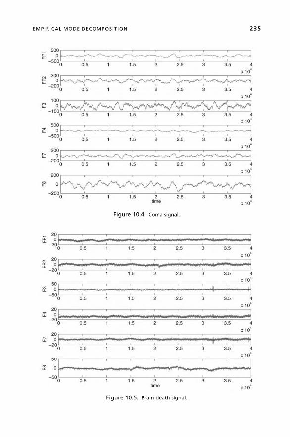
Figure 10.5. Brain death signal.

Figure 10.4. Coma signal.

EMPIRICAL MODE DECOMPOSITION 235

Sifting Algorithm

1. Find the local maxima and connect the maxima with interpolation (max

envelope). Also extract the minima and connect them by interpolation (min

envelope).

2. Take the average of the max envelope and the min envelope to determine the

signal mean.

3. Subtract the signal mean obtained from step 2 from the original signal.

4. Repeat steps 1, 2, and 3 until the signal satisfies the IMF criteria defined by

Huang [10].

5. Subtract the IMF signal from the original signal; a new signal is then obtained.

Again, steps 1, 2, 3, 4, and 5 should be implemented to extract IMFs until the

residual is a monotonic function.

The decomposition of a signal x(t) into IMFs can be summarized by the following

equation:

xðtÞ ¼Xni¼1ðCiðtÞÞþ rðtÞ ð10:2Þ

where Ci(t) is the ith IMF, n is the total number of IMFs, and r(t) is the residue.

The criteria of an IMF are as follows. The first condition is that the number of local

extrema and the number of zero crossings must either be equal or differ at most by one.

The second condition is that at any point the mean of the signal defined by the local

maxima and the local minima is zero.

10.5.2 The Hilbert Spectrum and Instantaneous Frequency

The monocomponent nature of the IMFs facilitates a unique time–frequency represen-

tation of the original signal—the Hilbert–Huang spectrum. The Hilbert transform is

T A B L E 10.2. EEG Signal Frequency Band

Frequency

Band

Frequency

(Hz) Consciousness Level Distribution

Delta 0.5–4 Low level of arousal Generally broad, diffused

Theta 4–8 Distracted Regional, involvesmany lobes

Alpha 8–12 Relaxed, meditation Regional, involves entire lobe

Low Beta 12–15 Relaxed, yet focused By side and lobe (frontal,

occipital, etc.)

Midrange Beta 15–18 Alert, active, not agitated Localized, over various areas

High Beta > 18 Very focused, alertness Very localized, maybe very

focused

Gamma 40 High-level info processing Very localized


given by [8]:

~xðtÞ ¼ H xðtÞ½ � ¼ð1�1

xðuÞpðt�uÞ du ð10:3Þ

wherex(t) is a time domain signal.H½ � � is the Hilbert operator. The analytic signal z(t) isrelated to the Hilbert transform of x(t), represented below as:

zðtÞ ¼ xðtÞþ j~xðtÞ ð10:4Þ

Given the analytic representation, the magnitude function a(t) and phase function u(t)can be obtained from z(t) as:

aðtÞ ¼ffiffiffiffiffiffiffiffiffiffiffiffiffiffiffiffiffiffiffiffiffiffiffiffiffiffix2ðtÞþ ~x2ðtÞ

qand uðtÞ ¼ arctan

~xðtÞxðtÞ� �

ð10:5Þ

zðtÞ ¼ aðtÞe juðtÞ ð10:6Þ

where a(t) describes the envelope of the original signal x(t), in the other words, the

instantaneous amplitude of the signal [8]. u(t) describes the instantaneous phase of x(t).Therefore, the instantaneous frequency of x(t) can be defined as the derivative of the

phase of the signal as:

wðtÞ ¼ d

dtuðtÞ ð10:7Þ

Thus, the Hilbert spectrum is given by [10]:

xðtÞ ¼Xni¼1

aiðtÞexp j

ðwiðtÞ

� �dt ð10:8Þ

Given the above representation equation, a three-dimensional plot with the amplitude,

instantaneous frequency as a function of time can be obtained in a straightforward

fashion. This is the Hilbert spectrum.

10.5.3 Importance of Complex EMD

The extension to the complex domainC is particularly important for the analysis of phase-dependent processes [15]. This applies not only to naturally occurring complex data, butalso to multi-channel real data. In this way, it is possible to analyze mutual phaseinformation between real-valued signals.

The first method of employing EMD in the complex domain, complex empirical

mode decomposition, was introduced in 2007 [19]. The method is rigorously derived,

based on the inherent relationship between the positive and negative frequency compo-

nents of a complex signal and the properties of theHilbert transform. The idea behind this

approach is rather intuitive: first note that a complex signal has a two-sided, asymmetric


spectrum. The complex signal can therefore be converted into a sum of analytic signals

by a straightforward filtering operation that extracts the opposite sides of the spectrum.

Direct analysis in C can be subsequently achieved by applying standard EMD to both thepositive and negative frequency parts of the signal. Given a complex signal x(k), real-valued components corresponding to the positive and negative sides of the spectrum can

be extracted as

xþ ðkÞ ¼ RF�1fXðe jwÞ �Hðe jwÞgx�ðkÞ ¼ RF�1fXðe jwÞ �Hðe�jwÞg

ð10:9Þ

whereF�1 is the inverse Fourier transform,R is an operator that extracts the real part of

a signal, and Hðe jwÞ is an ideal filter with the transfer function

Hðe jwÞ ¼ 1; w > 0

0; w < 0

�

Given that xþ (k) and x�(k) are real valued, standard EMD can be applied to obtain a set

of IMFs for each analytic signal. This can be expressed as

xþ ðkÞ ¼XMþi¼1

xiðkÞþ rþ ðkÞ

x�ðkÞ ¼X�1

i¼�M�xiðkÞþ r�ðkÞ

ð10:10Þ

where fxiðkÞgNþi¼1 and fxiðkÞgi¼1i¼�N� denote sets of IMFs corresponding, respectively,

to xþ (k) and x�(k), whereas rþ (k) and r�(k) are the respective residuals. The originalcomplex signal can be reconstructed by

x½ðkÞ ¼ ðxþ ðkÞþ jH½xþ ðkÞ�Þþ ðx�ðkÞþ jH½x�ðkÞ�Þ* ð10:11Þ

where H is the Hilbert transform operator. To conclude the derivation, a single set of

complex IMFs corresponding to the complex signal x(k) is given by

xðkÞ ¼XMþ

i¼M�; i „ 0yiðkÞþ rðkÞ ð10:12Þ

where r(k) is the residual and yi(k) is defined by

yiðkÞ ¼ðxþ ðkÞþ jH½xþ ðkÞ�Þ; i ¼ 1; . . . ;Mþ ;

ðx�ðkÞþ jH½x�ðkÞ�Þ*; i ¼ �M�; . . . ;�1

�

Although the two time series (x1(k) and x2(k)) are real valued, a complex signal,

z(k)¼ x1(k) þ jx2(k), is constructed with the signals representing the real and imag-

inary parts, respectively. To its advantage, it has a straightforward, intuitivemathematical


derivation. As an example of its mathematical robustness, it preserves the dyadic filter

property of standard EMD. In other words, the algorithm acts as dyadic filter bank when

processing complex noise [19].

Rotation-invariant EMD, introduced in [1], proposes a way of extending EMD

theory so that it operates fully in C. This is achieved through the use of complex splines.Unlike complex EMD, by design this method generates an equal number of IMFs for thereal and imaginary parts; these can be given physical meaning, thus retaining an importantproperty of real-valued EMD. A critical aspect of the derivation of EMD in C is thedefinition of an extremum. Several possible approaches are suggested in [1], such as the

extrema of the modulus and the locus where the angle of the first-order derivative (with

respect to time) changes sign; this way it can be assumed that local maxima will be

followed by local minima (and vice versa). This definition is equivalent to the extrema of

the imaginary part, that is, for a complex signal Z(t) (for convenience we here use a

continuous time index t):

ff _ZðtÞ ¼ 0Y fff _xðtÞþ j � _yðtÞg ¼ 0

Y tan�1_yðtÞ_xðtÞ ¼ 0Y _yðtÞ ¼ 0

ð10:13Þ

Because of its aforementioned advantages over complex EMD, namely the physical

meaning of its IMFs, rotation-invariant EMD is the extension of choice to perform

analysis on complex data.

10.5.4 Experiments and Results

As stated previously, an EEG signal can reflect brain activities; therefore, it is regarded as

a powerful tool to analyze cerebral consciousness status (e.g., coma and quasi-brain-

death). We distinguish cerebral consciousness status by analyzing EEG frequency

components within the frequency range from 0Hz to 30Hz; in particular, we are

interested (See Table 10.2) in the delta range (0.5 to 4Hz), theta range (4 to 8Hz),

alphawave (8 to 12Hz), and 13Hz componentswithin the lowbeta range. This is because

the patients are in a state of coma, as noted before, and this means that the brain activity

of interest dominates lower-frequency ranges.

We consider two patients (patient 1 and patient 2) in a coma state. EEG data for each

patient has been provided by [3]. Since these recordings were collected, patient 1 has a

wakened from coma while patient 2 has died. It is proposed to apply EMD to extract the

relevant features from the EEG data and to illustrate how these features can be used to

detect inevitable brain death in patient 2. Time–amplitude plots of length one second for

each of the six EEG channels (FP1, FP2, . . . , etc.) for patient 1 and patient 2 are given inthe left columns of Figures 10.6 and 10.7, respectively. EMD was applied to each of the

channels to decompose them into their IMFs and the resulting Hilbert spectrum was

computed. The Hilbert spectrum of each channel within the range 0 to 30Hz is given in

Figures 10.6 and 10.7, respectively. The third column of each figure shows the

frequency–amplitude plots for each channel obtained by averaging the corresponding

Hilbert spectrum plots.


Figure 10.7. Coma to Brain Death.

Figure 10.6. Coma to awake.


There are several important points to note regarding the features obtained using

EMD. First, it is clear that by comparing the frequency–amplitude plots for patient 1 and

patient 2, the brain activity within the range of 0 to 13Hz is significantly weaker for

patient 2. As mentioned earlier, activity within this range is related to the low level and

meditative brain activity. It can therefore be suggested that there is little or no activity

within this crucial range and that it can be used as an indication of inevitable brain death.

Also note that the same observations can be made from the data given in Figure 10.8,

patient 2 at a later date. The second point to note is that there exists strong similarity

between the spectra obtained from EEG channels of patient 1. For example, compare the

frequency–amplitude plots of FP1 and FP2 in Figure 10.6. However, it is clear that this is

not the case for patient 2. It can be thus concluded that strong similarities in the range 0 to

13Hz (particularly in channel FP1 and FP2) indicate that the patient will not succumb to

brain death.

10.5.4.1 EEG Phase Analysis using EMD. It is clear that if similarities exist

between specific frequency ranges (8 to 13Hz) among different EEG channels (FP1 and

FP2), then this is an indication that the patient will not succumb to brain death. For this

reason, it is proposed to extract relevant channel features using EMD and to compare

these features using complex extensions of the algorithm.

The EEG data from channel FP1 and FP2 for each patient were decomposed into

their IMFs and their instantaneous amplitude and frequencies were calculated. Features

within the desired frequency range were retained by [17], fusing instantaneous ampli-

tudes that corresponded to instantaneous frequencies within 8 to 13Hz. All other

Figure 10.8. Brain Death.


instantaneous amplitudes were omitted from the fusion process. The data was subse-

quently denoised [17] by zeroing the underlying signal if in a certain period, unless the

signal continuously has non-zero value in this period. The results of this fusion process

for FP1 andFP2 are given in the bottom panel of Figure 10.9 for patient 1. Similarly,

the fusion result for FP1 and FP2 for patient 2 is given in the bottom panel of Figure 10.10

0 1000 2000 3000 4000 5000 6000 7000 8000 9000−200

−100

0

100

200

Inpu

t−C

h1

0 1000 2000 3000 4000 5000 6000 7000 8000 9000−400

−200

0

200

400

Inpu

t−C

h2

0 1000 2000 3000 4000 5000 6000 7000 8000 90000

10

20

30

40

8−13

HZ

Am

p

time

Ch1Ch2

Figure 10.9. Filtered EEG deep coma patient 1 to awake.

0 1000 2000 3000 4000 5000 6000 7000 8000 9000−200

−100

0

100

200

Inpu

t−C

h1

0 1000 2000 3000 4000 5000 6000 7000 8000 9000−200

−100

0

100

Inpu

t−C

h2

0 1000 2000 3000 4000 5000 6000 7000 8000 90000

5

10

15

20

8−13

HZ

Am

p

time

Ch1Ch2

Figure 10.10. Filtered EEG deep coma patient 2 to death.


as FP10 and FP20, respectively. Note that among the features extracted for patient 1, there

is much synchronization between the extrema. This is not the case for patient 2.

Complex extensions of EMDwere then applied to the features so as to highlight any

synchronizations that were present. By decomposing the complex signal (FP10 þ jFP20)using rotation-invariant EMD, it was possible to monitor the phase relationship

accurately between the two channels. Taking the first complex IMF, it can be assumed

extracting the high-frequency information, which can suggest the spikes of the original

signal. By design, if the variations of two signals are similar, the phase of the complex

signal is approximately p/4. AS is shown in Figure 10.11, the panel represents the

absolutely value of the first complex IMF. The amplitude peaks when FP10 and FP20

both have a peak. The third plot in Figure 10.11 is a digitalized phase information. If the

phase of the first complex IMF is near top/4, thevaluewas set to one; otherwise, the valuewas set to zero. Then the extracted phase and amplitude information was combined

together by multiplying the absolute value of the first IMF with the digitalized phase

information. The combined amplitude–phase information can be seen from the plot at the

bottom of Figure 10.11. This is regarded as an index for detecting the amplitude–phase

similarity of the two signals. The result of the samemethod applied to the filtered signals

FP10 and FP20 is shown at the bottom of Figure 10.12.

By comparing the index derived from the coma signals of patient 1 and patient 2,

it can be seen that patient 1 is likely to recover. Note that the interval in the digitalized

phase information of patient 1 is longer than the interval in the digitalized phase

information of patient 2. This can suggest a quicker phase change in patient 2. Therefore,

the patient should be treated bymedical care rather than having further diagnosis tests for

braindeath.

Figure 10.11. Complex EEG analysis deep coma patient 1 leading to awake.


10.6 CONCLUSION

The data fusion via fission concept is introduced in this chapter. Using EMD as the

methodology of data fission, then fusing the information of interest, provides a powerful

tool for analyzing data. By extending EMD fusion via fission to the complex domain,

it can be seen that the methodology is not limited to complex signals, but is also useful

when the phase information between two signals is important. It has been illustrated in

the area of quasi-brain-death preliminary diagnosis.

10.7 REFERENCES

1. M. U. B. Altaf, T. Gautama, T. Tanaka, D.P. Mandic, “Rotation Invariant Complex Empirical

Mode Decomposition.” Proc. International Conference on Acoustics, Speech and Signal

Processing (ICASSP), 2007, Vol. 3, pp. 1009–1012.

2. H. K. Beecher, “A Definition of Irreversible Coma: Report of the Ad Hoc Committee of the

Harvard Medical School to Examine the Definition of Brain Death,” JAMA: Journal of the

American Medical Association, 205: 337–340, 1968.

3. J. Cao, “Analysis of the Quasi-Brain-Death EEG Data Based on a Robust ICA Approach,”

LNAI 4253, Part III: 1240–1247, KES 2006.

4. G. E. Chatrian, E. Lettich, P. L. Nelson, “Ten Percent Electrode System for Topographic

Studies of Spontaneous and Evoked EEG Activity,” American Journal of EEG Technology,

25: 83–92, 1985.

5. T. F. Collura, “The Five Percent Electrode System for High-Resolution EEG and ERP

Measurements,” Clinical Neurophysiology, 112: 713–719, 1997.

Figure 10.12. Complex EEG analysis deep coma patient 2 leading to brain death.


6. M.Datig, T. Schlurmann, “Performance andLimitations of theHilbert-Huang Transformation

(HHT) with an Application to Irregular Water Waves,” Ocean Engineering, 31: 1783–1834,

October 2004.

7. D.F. Group,“Functional Description of the Data Fusion Process,” Technical Report, Office of

Naval Technology, 1992.

8. S. L. Hahn, Hilbert Transforms in Signal Processing. Artech House, 1996.

9. D. L. Hall, J. Llinas, “An introduction to Multisensor Data Fusion.” Proc. IEEE, 1997, 85 (1):

6–23.

10. N. E. Huang, Z. Shen, S. R. Long, M. L. Wu, H. H. Shih, Z. Quanan, N. C. Yen, C. C. Tung,

H. H. Liu, “The Empirical Mode Decomposition and the Hilbert Spectrum for Nonlinear and

non-stationary Time Series Analysis,” Proc. Royal Society A, 1998, 454: 903–995.

11. H. H. Jasper. “Report of the Committee on Methods of Clinical Examination in electro-

encephalography,” Electroencephalography and Clinical Neurophysiology, (10): 370–375,

1958.

12. D. Looney, D. P. Danilo, “A Machine Learning Enhanced Empirical Mode Decomposition

(Accepted).”Proc. IEEEInt.Conf. onAcoustics, Speech, andSignalProcessing (ICASSP’O8),

2008.

13. D. Looney, L. Li, T. Rutkowski, D. P. Mandic, A. Cichocki, “Ocular Artifacts Removal from

EEG Using EMD.” First Int. Conf. Cognitive Neurodynamics, Shanghai, China, November

2007.

14. D. P. Mandic, M. Golz, A. Kuh, D. Obradovic, T. Tanaka, Signal Processing Techniques for

Knowledge Extraction and Information Fusion. Springer, 2008.

15. D. P. Mandic, G. Souretis, W. Leong, D. Looney, M. Hulle, T. Tanaka, Signal Process ing

Techniques for Knowledge Extraction and Information Fusion. Springer, 2007.

16. A. Paolin, A.Manuali, F. Di Paola, F. Boccaletto, P. Caputo, R. Zanata, G. P. Bardin, G. Simini,

“Reliability in diagnosis of brain death,” Intensive Care Med, 21: 657–662, 1995.

17. Y. Saito, T. Tanaka, J. Cao, D. P. Danilo, “Quasi-Brain-Death EEGData Ayalysis by Empirical

Mode Decomposition.” Proc. ICCN 2007.

18. G. Souretis, D. P. Mandic, M. Griselli, T. Tanaka, M. M. Van Hulle, “Blood Volume Signal

Analysis with Empirical Mode Decomposition.” Proc. 15th International DSP Conference,

2007, pp. 147–150.

19. T. Tanaka, D. P. Mandic, “Complex Empirical Mode Decomposition,” IEEE Signal Proces-

sing Letters, 14(2): 101–104, February 2007.

20. J. W. Tukey, Exploratory Data Analysis. Reading, MA: Addison-Wesley, 1977.

21. L. Wald, “Some Terms of Reference in Data Fusion.” IEEE Trans. Geosciences and Remote

Sensing, 37(3): 1190–1193, 1999.

22. E. Waltz, J. Llinas, Multisensor Data Fusion. Artech House, 1990.

23. R. R. Zhang, S.Ma, E. Safak, S.Hartzell, “Hilbert-HuangTransformAnalysis of Dynamic and

Earthquake Motion Recordings. J. Engineering Mechanics, 129: 861–875, 2003.

REFERENCES 245

11SIMILARITY ANALYSIS AND

KNOWLEDGE ACQUISITION BYUSE OF EVOLVING NEURAL

MODELS AND FUZZY DECISIONGancho Vachkov

Abstract: This chapter proposes a computational scheme for fuzzy similarity analysis

and classification of large data sets and images that first uses an information granulation

procedure followed by a subsequent fuzzy decision procedure. A special new version of

the growing unsupervised learning algorithm for information granulation is introduced in

the chapter. It reduces the original raw data (the RGB pixels) of the image to a

considerably smaller number of information granules (neurons). After that, two features

are extracted from each image: the center of gravity and theweighted average size of the

image. These features are further used as inputs of a special fuzzy inference procedure

that numerically computes the similarity degree for a given pair of images. Finally, a

sorting procedure with a predefined threshold is used to obtain the classification results

for all available images. The proposed similarity and classification scheme is illustrated

using the example of 18 images of flowers. The chapter also emphasizes that the

appropriate tuning of the parameters of the fuzzy inference procedure is quite important

for obtaining plausible, humanlike results. Therefore, a simple empirical process for

selection of these parameters is also suggested. Finally, the iterative computation scheme

for knowledge acquisition by using a gradually enlarging image base is also presented

and analyzed.


and Nikola Kasabov


11.1 INTRODUCTION

During the daily operation of many industrial systems and complex machines, such as

chemical and metallurgical plants, trucks, hydraulic excavators, and other construction

machines, large data sets can be collected from a number of sensors. These data sets are

later used bymaintenance engineers and experts to discover any significant difference or

change in the operating conditions, which points to a possible faulty condition of the

machine or system. If this is the case, quick countermeasures by the operator are needed

to prevent further deterioration in the system performance.

The above is only a small example of the many typical cases in which the human

operator is faced with the problem of similarity analysis of large multidimensional data

sets. Evaluating the similarity between a given set or pairs of large data sets and

discovering the differences between them is a very fundamental step that is used for

further classification and extracting a kind of knowledge about the system.

The complexity of the problem of similarity analysis arises from the fact that we

have to analyze and compare directly the large data sets to each other rather than just

classifying single patterns (single data points) in the predefined feature space, as in the

standard classification problem.

The problem of similarity exists also when different types of pictorial information

should be properly compared and classified. Here, the similarity analysis of a large

number of images is considered to be a very important step in themore general procedure

for unsupervised classification [1, 2] and knowledge acquisition from many types of

pictorial information.

This is a very specific and important task, where humans still perform better than the

currently available computerized systems. Among the reasons for such results are the

obvious complexity and thevagueness (subjective nature) of the problem itself, aswell as

the various possible criteria that could be used for the similarity analysis. Nevertheless, a

“good” (i.e., true and plausible) solution to the problem of similarity evaluation is a key

factor for success inmany applications, such as fast visual search through a large amount

of image information for proper sorting and classification.

In this chapter, we present a special fuzzy rule-based scheme for similarity analysis.

The results from this analysis, in the form of similarity degrees, can be later used for

unsupervised classification of images. After investigating several possible features for a

plausible similarity analysis, we have finally selected two of them as inputs of the fuzzy

decision procedure. These are the center of gravity of the image and the weighted

average size of the image, computed in two versions. The features are extracted from the

“raw” pixel data information through respective algorithms. Especially, the image

volume is approximately evaluated as the number of information granules (neurons)

that represent the original raw data set (pixels). The number of neurons, as well as their

proper locations in the three-dimensional RGB space, is automatically defined by a

specially introduced growing unsupervised learning algorithm.

Finally, extended simulations are performed over a test example, consisting of 18

images of different flowers. They show the merits of the proposed fuzzy rule-based

similarity analysis, which can be successfully applied to solving real-world classification

248 SIMILARITY ANALYSIS AND KNOWLEDGE ACQUISITION

problems that include much larger numbers of images. An iterative computation scheme

for knowledge acquisition based on a given image basewith core images is also presented

and discussed in the chapter.

11.2 BASICS OF INFORMATION GRANULATION

Normally, the large data sets and images are stored in the original “raw” form that keeps

all themeasurements or all pixels. In the case of image information, it is usually stored as

respective BMP or JPG file, where each pixel is represented by three integer numbers

within the range [0,255] that correspond to the intensity of the three basic colors Red,

Green and Blue. Thus thewhole image information is saved as a three-dimensional RGB

data set xi ¼ ½xi1; xi2; . . . ; xiK �; i ¼ 1; 2; . . . ;M, where K¼ 3 is the dimension number

and M represents the total number of pixels in this image.

However, it is obvious that directly using the original large raw RGB data set for

further processing is not the best idea from the point of view of efficient computation.

Therefore, we propose here another idea, according to the general concept of information

granulation in [3]. It is to replace the original large number of raw data with a smaller

number of “information granules,” by an appropriate unsupervised learning algo-

rithm [4–7]. The reduced set of information granules (called also neurons in this

chapter) is obtained by using the appropriate unsupervised learning algorithm, as will be

shown in the next sections. As a result of this learning, the set of neurons that is produced

should resemble as much as possible the density distribution, shape, and the volume of

the original set of RGB pixels in the three-dimensional space. This process is also called

information compression and the trained set of neurons is regarded as a kind of

compressed information model (CIM) or granulation model (GM) of the original (raw)

data set. It should be mentioned that such an approach to information compression

(granulation) that uses any of the unsupervised learning algorithms is a lossy compres-

sion in the sense that it would be not possible to fully recover the original information

from the obtained compressed model.

From a theoretical viewpoint, the information granulation can be considered as a

kind of unsupervised learning process that uses the original large three-dimensional data

set (containing M pixels): xi ¼ ½xi1; xi2; xi3�; i ¼ 1; 2; . . . ;M in order to determine the

locations of N information granules (neurons) in the same space, that is,

ci ¼ ½ci1; ci2; ci3�; i ¼ 1; 2; . . . ;N;N � Mwith CR¼M/N, called the compression ratio.

An illustrative example for information granulation is shown in the next two figures.

Figure 11.1 shows the original RGBdata set (4200 pixels) from a small image (not shown

here), whereas Figure 11.2. depicts the result of the information granulation, by using the

fixed number of N¼ 62 information granules (neurons) obtained after the end of the

unsupervised learning process.

Generally, the available unsupervised learning algorithms for information granu-

lation can be divided into three big groups:

Group 1, which consists of standard offline unsupervised learning algorithms with

the assumption of preliminary fixed number of neurons (granules) N, as in [5–7].

BASICS OF INFORMATION GRANULATION 249

Group 2,which uses the idea of the growing learning algorithm [8–10] with variable

(adjustable) number of neurons in order to fit a prespecified granulation quality.

Group 3, in which the concept of on-line unsupervised learning is used. Here it is

assumed that all data are not available at once but rather come “one by one” in a

finite (or even endless) sequence of data points. Then all neurons from the set of

assumed core neurons are gradually adjusting their locations in the space,

according to the newly arriving data. Our recent research results on this type

of online learning algorithm can be found in [10, 11].

Among the most popular standard offline learning algorithms from Group 1 are the

self-organizing (Kohonen) maps [4] and the neural gas learning algorithm [5]. One

modification of the offline neural gas learning algorithm is presented in Section 11.3.

0

50100

150200

250

050

100150

200250

050100150200250

050

100150

200

250

4200 Pixels

RedGreen

Blue

Figure 11.1. Three-dimensionalplotofa small image, containing4200pixelsusedas “raw”RGB

data set for information granulation.

0

50

100

150200

0

50

100150

200

050100150

200

250

050

100

150

200

250

RedGreen

Blue

Information Granulation with 62 Neurons

AVmin = 10

Figure 11.2. Information granulation with N¼62 neurons of the original RGB data set from

Figure 11.1.


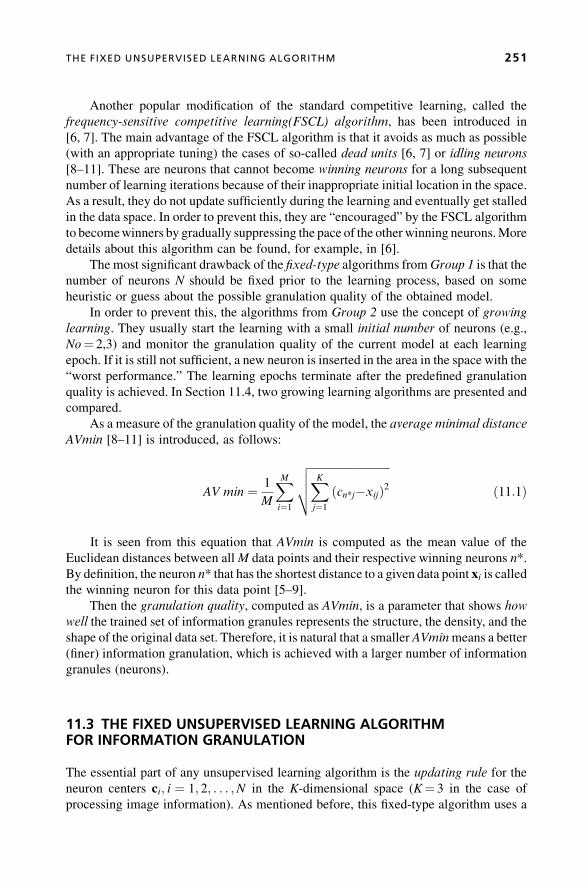
Another popular modification of the standard competitive learning, called the

frequency-sensitive competitive learning(FSCL) algorithm, has been introduced in

[6, 7]. The main advantage of the FSCL algorithm is that it avoids as much as possible

(with an appropriate tuning) the cases of so-called dead units [6, 7] or idling neurons

[8–11]. These are neurons that cannot become winning neurons for a long subsequent

number of learning iterations because of their inappropriate initial location in the space.

As a result, they do not update sufficiently during the learning and eventually get stalled

in the data space. In order to prevent this, they are “encouraged” by the FSCL algorithm

to becomewinners by gradually suppressing the pace of the other winning neurons.More

details about this algorithm can be found, for example, in [6].

The most significant drawback of the fixed-type algorithms fromGroup 1 is that the

number of neurons N should be fixed prior to the learning process, based on some

heuristic or guess about the possible granulation quality of the obtained model.

In order to prevent this, the algorithms from Group 2 use the concept of growing

learning. They usually start the learning with a small initial number of neurons (e.g.,

No¼ 2,3) and monitor the granulation quality of the current model at each learning

epoch. If it is still not sufficient, a new neuron is inserted in the area in the space with the

“worst performance.” The learning epochs terminate after the predefined granulation

quality is achieved. In Section 11.4, two growing learning algorithms are presented and

compared.

As a measure of the granulation quality of the model, the average minimal distance

AVmin [8–11] is introduced, as follows:

AV min ¼ 1

M

XMi¼1

ffiffiffiffiffiffiffiffiffiffiffiffiffiffiffiffiffiffiffiffiffiffiffiffiffiffiffiffiffiXKj¼1ðcn*j�xijÞ2

vuut ð11:1Þ

It is seen from this equation that AVmin is computed as the mean value of the

Euclidean distances between allM data points and their respective winning neurons n*.

By definition, the neuron n* that has the shortest distance to a given data point xi is calledthe winning neuron for this data point [5–9].

Then the granulation quality, computed as AVmin, is a parameter that shows how

well the trained set of information granules represents the structure, the density, and the

shape of the original data set. Therefore, it is natural that a smaller AVminmeans a better

(finer) information granulation, which is achieved with a larger number of information

granules (neurons).

11.3 THE FIXED UNSUPERVISED LEARNING ALGORITHMFOR INFORMATION GRANULATION

The essential part of any unsupervised learning algorithm is the updating rule for the

neuron centers ci; i ¼ 1; 2; . . . ;N in the K-dimensional space (K¼ 3 in the case of

processing image information). As mentioned before, this fixed-type algorithm uses a

THE FIXED UNSUPERVISED LEARNING ALGORITHM 251

predetermined number of neuronsN and the updating rule is performed for a preliminary

fixed number of T iterations (t¼ 0, 1, 2, . . ., T), as follows:

ciðtÞ ¼ ciðt�1ÞþDciðtÞ; i ¼ 1; 2; . . . ;N ð11:2Þ

Here the computation way of the updateDciðtÞ varies according to the version of theunsupervised algorithm, such as [4–8].We use here a special simplified version [8–10] of

the original neural gas learning algorithm [5], where the amount of the update is

computed as:

DciðtÞ ¼ RðtÞHsðt; riÞ½xs�ciðt�1Þ�;i ¼ 1; 2; . . . ;N; s ¼ 1; 2; . . . ;M

ð11:3Þ

The parameter RðtÞ; 0 � RðtÞ � 1; t ¼ 0; 1; 2; . . . ; T in (11.3) is a monotonically

decreasing learning rate,which guarantees the convergence and stability of the learning

process:

RðtÞ ¼ R0 expð�t=TCÞ; t ¼ 0; 1; . . . ; T ð11:4Þ

The neighborhood function 0 � Hsðt; riÞ � 1 in (11.3) also decreases exponentially

with the iterations. It is used to compute the dynamic activity of all neurons, which

decreases exponentially with the iterations and depends also on the current ranking order

of the neuron at this iteration. In [4–8], we proposed a simple way to compute the

monotonically decreasing neighborhood function as follows:

Hsðt; riÞ ¼ exp½�ðri�1Þ=BðtÞ�;t ¼ 0; 1; . . . ; T ; s ¼ 1; 2; . . . ;M; i ¼ 1; 2; . . . ;N

ð11:5Þ

where

BðtÞ ¼ expð�t=TWÞ; t ¼ 0; 1; . . . ;T ð11:6Þ

Here ri 2 ½1; 2; . . . ;N� is an integer number for the ranking order of the ith neuron

(i¼ 1, 2, . . .,N) to the sth data point (s¼ 1, 2, . . .,M). This ranking order is defined by the

Euclidean distance between the ith neuron and the sth data point. The closest neuron (in

the sense of minimal Euclidean distance) is called the winning neuron and gets ranking

order r¼ 1. The second closest neuron gets r¼ 2, and so on.

The initial learning rate R0 and the steepness parameters TC and TW have to be

preset before the learning. In the further simulation we use the following settings:

T ¼ 500;R0 ¼ 0:15 and TC ¼ TW ¼ T=5: One typical example for information com-

pression of a raw data set containing M¼ 800 data by using N¼ 60 neurons is given in

Figure 11.3.

The unsupervised learning algorithm described above is referred to as algorithm

Fixed when compared to the next two learning algorithms presented in Section 11.4.


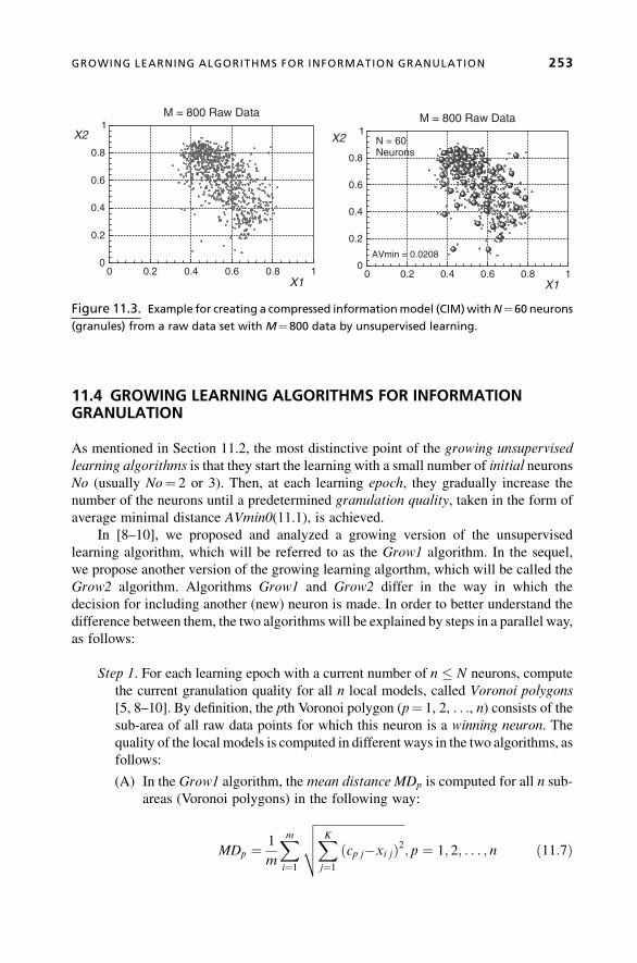
11.4 GROWING LEARNING ALGORITHMS FOR INFORMATIONGRANULATION

As mentioned in Section 11.2, the most distinctive point of the growing unsupervised

learning algorithms is that they start the learning with a small number of initial neurons

No (usually No¼ 2 or 3). Then, at each learning epoch, they gradually increase the

number of the neurons until a predetermined granulation quality, taken in the form of

average minimal distance AVmin0(11.1), is achieved.

In [8–10], we proposed and analyzed a growing version of the unsupervised

learning algorithm, which will be referred to as the Grow1 algorithm. In the sequel,

we propose another version of the growing learning algorthm, which will be called the

Grow2 algorithm. Algorithms Grow1 and Grow2 differ in the way in which the

decision for including another (new) neuron is made. In order to better understand the

difference between them, the two algorithms will be explained by steps in a parallel way,

as follows:

Step 1. For each learning epoch with a current number of n � N neurons, compute

the current granulation quality for all n local models, called Voronoi polygons

[5, 8–10]. By definition, the pth Voronoi polygon (p¼ 1, 2, . . ., n) consists of thesub-area of all raw data points for which this neuron is a winning neuron. The

quality of the local models is computed in different ways in the two algorithms, as

follows:

(A) In the Grow1 algorithm, the mean distance MDp is computed for all n sub-

areas (Voronoi polygons) in the following way:

MDp ¼ 1

m

Xmi¼1

ffiffiffiffiffiffiffiffiffiffiffiffiffiffiffiffiffiffiffiffiffiffiffiffiffiffiffiffiffiXKj¼1ðcp j�xi jÞ2

vuut ; p ¼ 1; 2; . . . ; n ð11:7Þ

10.80.60.40.200

0.2

0.4

0.6

0.8

1M = 800 Raw Data

X1

X2

10.80.60.40.200

0.2

0.4

0.6

0.8

1M = 800 Raw Data

X1

X2 N = 60 Neurons

AVmin = 0.0208

Figure 11.3. Example for creating a compressed informationmodel (CIM)withN¼60 neurons

(granules) from a raw data set with M¼800 data by unsupervised learning.

GROWING LEARNING ALGORITHMS FOR INFORMATION GRANULATION 253

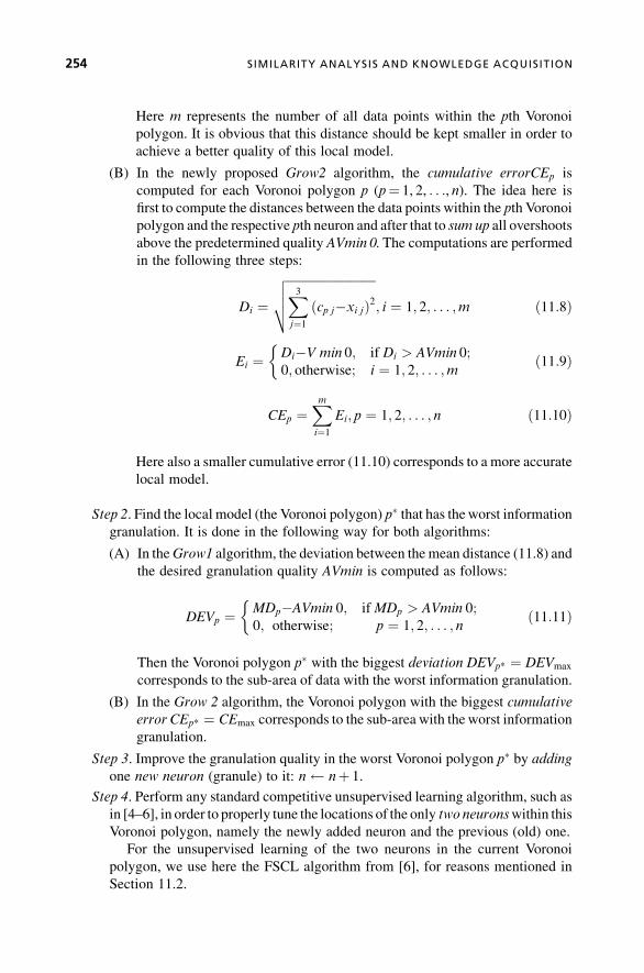
Here m represents the number of all data points within the pth Voronoi

polygon. It is obvious that this distance should be kept smaller in order to

achieve a better quality of this local model.

(B) In the newly proposed Grow2 algorithm, the cumulative errorCEp is

computed for each Voronoi polygon p (p¼ 1, 2, . . ., n). The idea here is

first to compute the distances between the data points within the pth Voronoi

polygon and the respective pth neuron and after that to sum up all overshoots

above the predetermined quality AVmin 0. The computations are performed

in the following three steps:

Di ¼ffiffiffiffiffiffiffiffiffiffiffiffiffiffiffiffiffiffiffiffiffiffiffiffiffiffiffiffiffiX3j¼1ðcp j�xi jÞ2

vuut ; i ¼ 1; 2; . . . ;m ð11:8Þ

Ei ¼ Di�V min 0; if Di > AVmin 0;0; otherwise; i ¼ 1; 2; . . . ;m

�ð11:9Þ

CEp ¼Xmi¼1

Ei; p ¼ 1; 2; . . . ; n ð11:10Þ

Here also a smaller cumulative error (11.10) corresponds to a more accurate

local model.

Step 2. Find the local model (the Voronoi polygon) p� that has theworst information

granulation. It is done in the following way for both algorithms:

(A) In theGrow1 algorithm, the deviation between themean distance (11.8) and

the desired granulation quality AVmin is computed as follows:

DEVp ¼ MDp�AVmin 0; if MDp > AVmin 0;0; otherwise; p ¼ 1; 2; . . . ; n

�ð11:11Þ

Then the Voronoi polygon p� with the biggest deviation DEVp* ¼ DEVmax

corresponds to the sub-area of data with the worst information granulation.

(B) In the Grow 2 algorithm, the Voronoi polygon with the biggest cumulative

error CEp* ¼ CEmax corresponds to the sub-area with theworst information

granulation.

Step 3. Improve the granulation quality in the worst Voronoi polygon p� by addingone new neuron (granule) to it: n nþ 1.

Step 4. Perform any standard competitive unsupervised learning algorithm, such as

in [4–6], in order to properly tune the locations of the only two neuronswithin this

Voronoi polygon, namely the newly added neuron and the previous (old) one.

For the unsupervised learning of the two neurons in the current Voronoi

polygon, we use here the FSCL algorithm from [6], for reasons mentioned in

Section 11.2.


Step 5. Check the granulation quality (11.1) of the whole model, achieved by the

current number of n neurons. If AVmin � AVmin0, then the predetermined

quality is achieved with N ¼ n neurons and the algorithm terminates. If

AVmin > AVmin0, the algorithm continues the learning process with the next

epoch from step 1.

11.5 COMPARISON OF THE GROWING AND THE FIXED LEARNINGALGORITHMS FOR INFORMATION GRANULATION

It is worth noting that the learning process of the growing algorithms is much faster (as

computation time) compared with the fixed-type learning algorithm from Section 11.3.

There are two reasons for this. The first one is that, here, instead of the whole data set

containing allM data, amuch smaller subset of onlym<M data is used for the learning at

each epoch. This subset consists of the data points that belong to the current, worst sub-

area p�. The second reason for the faster performance is that at each learning epoch, only

two neurons are used, instead of thewhole set ofN neurons, as in the case of the algorithm

Fixed.

We compared all three learning algorithms, namely Fixed, Grow1, and Grow2, in

the same example of a large data set, consisting of M¼ 49152 three-dimensional data.

This data set was actually the RGB pixels matrix from an image (image 4 from

Figure 11.6) with resolution 256 192 pixels. For a predetermined granulation quality

of AVmin¼ 12, number of iterations T¼ 350, and learning rate R0 ¼ 0:11, the CPU time

(using the same compiler) was as follows: 119 sec for Grow1, 177 sec for Grow2, and

257 sec for Fixed. At the end of the learning, the number of all generated neurons was as

follows:N¼ 109 forGrow1 andN¼ 169 forGrow2. The algorithmFixedwas runwith a

predetermined number of N¼ 109 neurons. Figure 11.4 shows the convergence of the

AVmin for both algorithms. It becomes clear that Grow2 is the fastest among the three

16014012010080604020010

15

20

25

30

35

40

45

50

55AVmin

Epochs

Grow1Grow2

Comparison of Grow1 and Grow2Algorithms

Figure 11.4. Convergence of the granulation quality AVmin for Grow1 and Grow2.

COMPARISON OF THE GROWING AND THE FIXED LEARNING ALGORITHMS 255

algorithms and, additionally, it produces a more economical model with the same

granulation quality AVmin by using a smaller number of neurons than Grow1.

Figure 11.5 shows the amount of data that are used for learning at each epoch for both

growing learning algorithms:Grow1 andGrow2. Note that after the first epoch that uses

the full set ofM¼ 49152 data, all other epochs use only a fraction of these data, located in

the worst sub-area of the data space. In addition, this number tends to decrease

exponentially with the growing number of epochs. This fact explains the speed of the

growing algorithms, compared with the algorithm Fixed, which always uses the full set

of data.

However, the algorithm Fixed produces a granulation model (gm) with a slightly

better granulation quality AVmin, compared with any of the growing algorithms that use

the same number of neurons. For example, algorithm Grow1 produces a model with

AVmin¼ 11.987 by usingN¼ 109 neutrons. At the same time, algorithmFixed creates a

granulation model with the same fixed number of N¼ 109 neurons, but with a better

granulation quality of AVmin¼ 11.463. Even if the difference is not so significant, it is a

matter of a trade-off (CPU time against themodel quality) whenmaking a decision about

the proper algorithm for information granulation.

Finally, the growing learning algorithmsGrow1 andGrow2 can be considered to be

a kind of adaptive algorithms that gradually adjust both the number and the position of

the neurons so as to reach the predetermined model quality AVmin. From such a point of

view, these algorithms gradually build evolving models, during the learning process.

Since we use an offline data set with a fixed number of data (M¼ const), this allows us to

perform iterations over the whole available data set and to evolve the models during the

iterations. As a result, the final models that are produced will be fitted to the concrete

training data set but cannot be used for another data set with different characteristics.

From such a point of view, themodels produced by the offline data set cannot be regarded

as fully evolving models.

1801601401201008060402000

5,000

10,000

15,000

20,000

25,000

30,000

35,000

40,000

45,000

50,000

Learning Epochs

Number of Data Used at Each Epoch

Algorithms: Grow1 and Grow2

Algorithm: Fixed

Figure 11.5. Number of data used for learning at each epoch for algorithmsGrow1 andGrow2

compared with algorithm Fixed.


11.6 SELECTION OF FEATURES FOR THE SIMILARITY ANALYSIS

The unsupervised classification of images [1, 2] can be viewed as a simple computational

procedure that uses the results of the preliminary similarity analysis, namely the

computed similarity degrees between the new (unknown) image and all existing images

from the image base. For classification purposes, these results have to be sorted in

descending order of the similarity degrees for each pair of images. Then, according to a

preliminary, assumed reasonable threshold for the similarity degree, the new (unknown)

image is classified as “belonging” to the class of the “most similar” image or rejected as

“non-belonging” to any known class of images.

Now it becomes clear that in order to achieve a satisfactory solution to this problem

wefirst need to extract themost representative characteristics (features) from the original

images in appropriate numerical form that corresponds to the specific of this image.

We can view each separate image as a kind of data cloud in the three-dimensional

RGB space, which has its specific density distribution, shape, and location in this space.

All three correspond in some indirect way to the diversity and the overall ratio of the

colors in the original two-dimensional image. Therefore, the problem of computing

the similarity degree between a given pair of images becomes a problemof evaluating the

difference between the respective features of the three-dimensional data clouds in the

RGB space.

It seems natural to assume that the first (and probably the most important) feature

that can be extracted from a given data cloud is its center of gravity (COG), defined as the

vector CG ¼ CG1;CG2;CG3½ �, which can be directly computed from the original raw

data as follows:

CGj ¼XMi¼1

xi j=M; j ¼ 1; 2; 3 ð11:12Þ

If the original raw data are already not available (after the information granulation),

then the center of gravity can be also approximately evaluated by using the parameters of

the obtained granulation model, in the following way:

CGj ¼XNi¼1

ci jgi=XNi¼1

gi; j ¼ 1; 2; 3 ð11:13Þ

Here, 0 < gi � 1; i ¼ 1; 2; . . . ;N are the normalized weights of the neurons,

computed as:

gi ¼ mi=M; i ¼ 1; 2; . . . ;N ð11:14Þ

and mi � M; i ¼ 1; 2; . . . ;N is the number of the data points: xs; s ¼ 1; 2; . . . ;mi for

which the ith neuron is a winning neuron.

It is obvious that there will be a slight difference between the real COG computed

by (11.12) and its evaluated value, computed by (11.13). This discrepancy is related to the

SELECTION OF FEATURES FOR THE SIMILARITY ANALYSIS 257

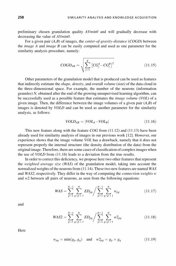
preliminary chosen granulation quality AVmin0 and will gradually decrease with

decreasing the value of AVmin0.

For a given pair (A,B) of images, the center-of-gravity-distance (COGD) between

the image A and image B can be easily computed and used as one parameter for the

similarity analysis procedure, namely:

COGDAB ¼ffiffiffiffiffiffiffiffiffiffiffiffiffiffiffiffiffiffiffiffiffiffiffiffiffiffiffiffiffiffiffiffiffiffiffiffiXKj¼1

�CGA

j �CGBj

�2vuut ð11:15Þ

Other parameters of the granulation model that is produced can be used as features

that indirectly estimate the shape, density, and overall volume (size) of the data cloud in

the three-dimensional space. For example, the number of the neurons (information

granules) N, obtained after the end of the growing unsupervised learning algorithm, can

be successfully used as a possible feature that estimates the image volume (VOL) of a

given image. Then, the difference between the image volumes of a given pair (A,B) of

images is denoted by VOLD and can be used as another parameter for the similarity

analysis, as follows:

VOLDAB ¼ VOLA�VOLBjj ð11:16Þ

This new feature along with the feature COG from (11.12) and (11.13) have been

already used for similarity analysis of images in our previous work [12]. However, our

experience shows that the image volume VOL has a drawback, namely that it does not

represent properly the internal structure (the density distribution of the data) from the

original image. Therefore, there are some cases of classification of complex imageswhen

the use of VOLD from (11.16) leads to a deviation from the true results.

In order to correct this deficiency, we propose here two other features that represent

the weighted average size (WAS) of the granulation model, taking into account the

normalizedweights of the neurons from (11.14). These two new features are namedWAS

andWAS2, respectively. They differ in the way of computing the connection weights w

and w2 between all pairs of neurons, as seen from the following equations:

WAS ¼XN�1p¼1

XNq¼pþ 1

EDpq

�XN�1p¼1

XNq¼pþ 1

wpq ð11:17Þ

and

WAS2 ¼XN�1p¼1

XNq¼pþ 1

EDpq

�XN�1p¼1

XNq¼pþ 1

w2pq ð11:18Þ

Here

wpq ¼ minðgp; gqÞ and w2pq ¼ gp gq ð11:19Þ


denote the connection weights for a given pair fp; qg of neurons, and EDpq in (11.17)

and (11.18) is the Euclidean Distance between the neurons in this pair.

The differences WASD and WAS2D between the respective weighted average

sizes (11.17) and (11.18) for a given pair (A,B) of images can be used as two other

parameters for the similarity analysis, as follows:

WASDAB ¼ WASA�WASBjj ð11:20Þ

WAS2DAB ¼ WAS2A�WAS2Bjj ð11:21Þ

Performance analysis of the classification, made by using all four parameters,

computed by (11.15), (11.6) and (11.20), (11.21), is shown and discussed in the next

sections.

11.7 EXAMPLE OF SIMILARITY ANALYSIS OF IMAGES

In order to illustrate the whole proposed process for image classification, based on

similarity analysis, later we use the following test example of 18 images, representing

different flowers, as shown in Figure 11.6.

As mentioned in Section 11.2, first the BMP files with the original images have been

preprocessed in order to obtain the respective RGB files with the raw data in the form of

three-dimensional matrixes containing the pixel values within the range of 0–255.

The center of gravity CG of all 18 images from Figure 11.6. have been computed

from the rawpixel data byusing equation (11.12).Their locations in the three-dimensional

RGB space are shown in Figure 11.7. They almost coincide with the locations of the CG

obtained from the respective granulation models and computed by (11.13).

It is easy to see in Figure 11.7 that the CGs for many of the images are quite close to

each other, that is, they can be considered to be very similar. However, this differs from

the reality, as seen from the original images in Figure 11.6. Therefore, a conclusion can

bemade that the use of only one feature (the center of gravity in this case) is not sufficient

for a true and precise similarity analysis and classification.

The image volumes VOL for all 18 images have been computed by both learning

algorithms,Grow1 andGrow2, and for three desired values of the granulation quality, as

follows: AVmin0¼ 12, 13, and 14. The results from using the Grow2 algorithm are

shown in Figure 11.8. It is seen from this figure that the ratio between the image volumes

of the different images remains almost unchanged with increasing or decreasing

granulation quality AVmin0. This means that even larger (faster-computed) values of

AVmin0 could be used with the same success for the similarity analysis.

A direct comparison between algorithmsGrow1 andGrow2 is shown in Figure 11.9

for the same granulation quality AVmin0¼ 12. Note that the Grow2 algorithm reaches

the same (predetermined) granulation quality AVmin0 by using fewer neurons; that is, it

produces a more economical solution to the granulation problem. The general reason for

such a result is that the cumulative error (11.10) gives amore precise characteristic of the

model than the mean distance (11.7).

EXAMPLE OF SIMILARITY ANALYSIS OF IMAGES 259

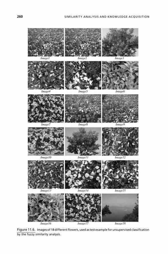
Figure 11.6. Imagesof18differentflowers,usedas testexample forunsupervised classification

by the fuzzy similarity analysis.


Figure 11.10 depicts the next two features, namely the weighted average sizesWAS

(11.17) andWAS2(11.18) for all 18 test images. In the figure, these two features follow

the same (increase–decrease) tendency, which means that we expect similar results from

them for the similarity analysis.

Each of the above four features have been used separately for similarity analysis and

classification, by computing the respective distances: (11.15), (11.16), (11.20),

and (11.21). The results are shown in Table 11.1. Here N1 and N2 denote the most

similar and the second-most-similar image.

It is easy to note the discrepancy between the results produced by each feature

separately.

The results from this similarity analysis lead to the conclusion that using each of the

four single features separately does not produce plausible results for all test examples

1816141210864200

20

40

60

80

100

120N—Number of Neurons Grow2 Algorithm

Images

AVmin=14

AVmin=12

AVmin=13

Figure 11.8. Image volumes VOL (number of neurons N) of all 18 Images from Figure 11.6,

computed by learning algorithm Grow2.

90100

110120

130140

150

2040

6080

100120

140160

80

100

120

140

160

80

100

120

140

160

Center-of-Gravity of All 18 Models

RedGreen

Blue

Figure 11.7. Centers of gravityCGof all 18 Images fromFigure 11.6, computedby (11.12). They

almost coincide with the CG computations by (11.13).

EXAMPLE OF SIMILARITY ANALYSIS OF IMAGES 261

1816141210864200

50

100

150

200 Grow1

Grow2

N—Number of Neurons

Images

AVmin = 12

Figure 11.9. Image volumesVOLof all 18 Images from Figure 11.6, computedby both learning

algorithms:Grow1 andGrow2. Note that theGrow2 algorithmproduces amore efficientmodel

for the same desired AVmin.

T A B L E 11.1. Four Different Classifications of All 18 Images, Performed by Using SeparatelyAll Four Single Features

Four “Single-Feature” Classifications

COGD

(11.15)

VOLD

(11.16)

WASD

(11.20)

WAS2D

(11.21)

Image N1 N2 N1 N2 N1 N2 N1 N2

1 9 8 8 14 2 9 8 2

2 10 6 6 16 9 1 9 1

3 14 15 6 16 11 13 13 18

4 13 12 5 15 12 18 12 18

5 15 14 4 15 15 7 11 14

6 16 10 16 3 16 9 16 9

7 17 15 17 11 17 11 17 15

8 9 1 1 14 10 1 1 2

9 1 8 14 1 2 1 2 1

10 2 16 2 6 8 18 8 4

11 12 4 3 17 17 3 5 15

12 4 13 5 4 4 18 18 13

13 4 12 15 4 4 3 18 12

14 3 15 9 1 15 5 5 11

15 5 17 13 4 5 14 7 17

16 6 10 16 3 6 9 6 9

17 7 15 7 11 11 7 7 15

18 13 4 7 17 12 4 12 13


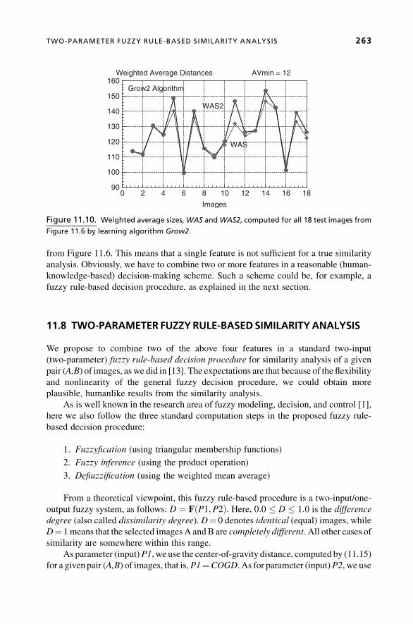
from Figure 11.6. This means that a single feature is not sufficient for a true similarity

analysis. Obviously, we have to combine two or more features in a reasonable (human-

knowledge-based) decision-making scheme. Such a scheme could be, for example, a

fuzzy rule-based decision procedure, as explained in the next section.

11.8 TWO-PARAMETER FUZZYRULE-BASEDSIMILARITYANALYSIS

We propose to combine two of the above four features in a standard two-input

(two-parameter) fuzzy rule-based decision procedure for similarity analysis of a given

pair (A,B) of images, as we did in [13]. The expectations are that because of the flexibility

and nonlinearity of the general fuzzy decision procedure, we could obtain more

plausible, humanlike results from the similarity analysis.

As is well known in the research area of fuzzy modeling, decision, and control [1],

here we also follow the three standard computation steps in the proposed fuzzy rule-

based decision procedure:

1. Fuzzyfication (using triangular membership functions)

2. Fuzzy inference (using the product operation)

3. Defiuzzification (using the weighted mean average)

From a theoretical viewpoint, this fuzzy rule-based procedure is a two-input/one-

output fuzzy system, as follows: D ¼ FðP1;P2Þ. Here, 0:0 � D � 1:0 is the difference

degree (also called dissimilarity degree). D¼ 0 denotes identical (equal) images, while

D¼ 1means that the selected images A andB are completely different. All other cases of

similarity are somewhere within this range.

As parameter (input)P1, we use the center-of-gravity distance, computed by (11.15)

for a given pair (A,B) of images, that is,P1¼COGD. As for parameter (input)P2, we use

18161412108642090

100

110

120

130

140

150

160

Images

AVmin = 12

Grow2 Algorithm

WAS2

WAS

Weighted Average Distances

Figure 11.10. Weighted average sizes,WAS andWAS2, computed for all 18 test images from

Figure 11.6 by learning algorithm Grow2.

TWO-PARAMETER FUZZY RULE-BASED SIMILARITY ANALYSIS 263

the weighted average size differences, computed by (11.20) and also by (11.21). Since

the results obtained from the similarity analysis using WASD and those using WAS2D

were similar, we will display the results by using P2¼WAS2D.

For each of the inputs P1 and P2, we have assumed five triangular membership

functions for the fuzzification step. Their respective linguistic variables are: VS¼Very

Small; SM¼ Small; MD¼Medium; BG¼Big; and VB¼Very Big.

It is well known that the general problem in fuzzy modeling, control, and decision is

the proper tuning of the locations (centers) of all membership functions. Here different

optimization techniques could be applied to successfully tune the membership function

locations, with a preliminary defined optimization criterion.

In this chapter we are not dealing with the problem of precise tuning and the choice

of the optimization criterion. We are rather interested in investigating and showing how

sensitive are the preliminary chosen parameters P1 and P2 to the final results from the

similarity analysis. For this purpose in the sequel we propose a kind of simple heuristic

(and approximate) computational procedure for finding the range and the centers of the

membership functions for P1 and P2.

First, we compute the ranking lists P1min ! P1max and P2min ! P2max for

each image separately, compared to all other images. The results from these computa-

tions for the test example with 18 images is shown in Figure 11.11 for parameter

P1¼COGD and in Figure 11.12 for parameter P2¼WAS2D.

After that, the centers of each linguistic variable are computed according to the

following (heuristic) rule:

VS¼ 0.0

SM¼Mean value of Rank No. 2 for all images

MD¼Mean value of Rank No. 5 for all images

BG¼Mean value of Rank No. 9 for all images

VB¼Mean value of Rank No. 17 (the most different image)

1816141210864200

20

40

60

80

100

120

140

160

P1 = COGD Center-of-Gravity Distance

Images

Rank No. 1,2,3,4, and 5

COGD = max

Figure 11.11. Ranking list for all 18 images, using parameter P1¼COGD(11.15).


The computed centers of the triangular membership functions for parameters P1 and P2

are shown in the three charts in Figure 11.13.

The next important block in the fuzzy decision procedure is the fuzzy rule base. As

shown in Figure 11.14, it consists of 25 human-experience-based fuzzy rules, with

singleton-type (numerical) outputs denoted by U1;U2; . . . ;U9.

The following numerical values for all nine singletons U1;U2; . . . ;U9 have been

assumed in this simulation:

U1 ¼ 0:0;U2 ¼ 0:125;U3 ¼ 0:250;

U4 ¼ 0:375;U5 ¼ 0:500;U6 ¼ 0:625;

U7 ¼ 0:750;U8 ¼ 0:875;U9 ¼ 1:0

ð11:22Þ

It isworth noting that any changes in their values could produce different final results

from the similarity analysis, so these are important tuning parameters, too.

The response surface of the fuzzy inference procedure that uses the fuzzy rule base

from Figure 11.14 and the membership functions from Figure 11.13 is shown in

Figure 11.15.

This response surface is computed by the following defuzzification procedure:

D ¼XLi¼1

uivi

�XLi¼1

vi ð11:23Þ

Here, 0 � vi � 1; i ¼ 1; 2; . . . ; L is the firing (activation) degree of the ith fuzzy rule

and L¼ 25 is the total number of fuzzy rules. ui 2 ½U1;U2; . . . ;U9� represents the

actual singleton value of the ith fuzzy rule, according to the fuzzy rule base in

Figure 11.14, for example, u8 ¼ U4 ¼ 0:375, since fuzzy rule 8 as seen fromFigure 11.14

1816141210864200

10

20

30

40

50

60

Rank No. 1,2,3,4 and 5

WAS2D = max

P2 = WAS2D WAS2 Difference

Images

Figure 11.12. Ranking list of all 18 images, using parameter P2¼WAS2D(11.21).


1201008060402000

0.2

0.4

0.6

0.8

1

Membership Value for COG_Distance

P1 = COG Distance

MDSMVS BG VB

353025201510500

0.2

0.4

0.6

0.8

1

P2 = WAS_Difference

Membership Value for WAS_DifferenceVS MDSM BG VB

40353025201510500

0.2

0.4

0.6

0.8

1

P2 = WAS2_Difference

Membership Value for WAS2_DifferenceBGMDSMVS VB

Figure 11.13. Five triangular membership functions assumed for inputs P1 and P2.


is as follows:

IFðF1 is SMAND F2 isMDÞ THEND ¼ U4 ð11:24Þ

The results from the similarity analysis based on the above-proposed fuzzy decision

procedure are discussed below.

Table 11.2 shows the three most similar results ranked as no.1, no. 2, and no. 3, for

each of the 18 test images. Here, the two input parameters used for the fuzzy decision are

P1¼COGD and P2¼WAS2D. N1, N2, and N3 denote the code numbers of the image

and FD1, FD2, and FD3 are the fuzzy difference degrees D computed by (11.23).

A detailed look at the results shows that, in most cases, the images that are ranked as

no. 1 (themost similar images) represent the correct similarity decision, which coincides

with the human decision. However, there are also some cases, such as the similarity

decisions for images 3 and 13, that do not look correct from a human viewpoint. These

two images represent different parts of the same tree and, according to the commonsense

human decision, this pair of images should be considered to be the most similar images.

However, the fuzzy decision procedure shows different results in Table 11.2.

This fact also shows that a proper human-defined criterion for similarity should

be established prior to running a respective optimization procedure that tunes the para-

meters of the fuzzy decision procedure, namely, the centers of the membership functions

andthevaluesofthesingletons.Then,thecomputerfuzzydecisionprocedureshouldbeable

to closely simulate the human similarity decision. Our future research goal lies in this

direction.

Another important finding from Table 11.2 is that even if an image has been

classified as no. 1 (i.e., the most similar image to a given one), the final decision for

acceptance or rejection of this result should be made using a prespecified threshold, Th.

For example, if the preset threshold is Th¼ 0.33, then the solutions for the similarity

analysis of images nos. 3, 10, 11, and 18 would be discarded as nonplausible, that is,

image no. 18 is not similar to image no. 12, even if it is ranked as no. 1.

VS

SM

MD

BG VBVS MD

BG

VB

F1

P2

WAS(WAS2)Difference

Center-of-Gravity Distance

Fuzzy Difference between Two Images

SM

D

U2

U1

U3

U4

U5

U2

U3

U4

U5

U6

U4U3 U5

U4

U5

U6

U7

U5

U6

U7

U8

U6

U7

U8

U9

Figure 11.14. Proposed fuzzy rule base (FRB) with 25 fuzzy rules, used for similarity analysis.


11.9 UNSUPERVISED CLASSIFICATION FOR KNOWLEDGEACQUISITION

The above-proposed computation scheme for similarity analysis can be incorporated into

a larger computation scheme for classification of new (unknown, test) images to a given

image base that contains the group of currently known core images. These images are

considered to be available current pieces of knowledge about the process under

investigation. The block diagram of this computation scheme is shown in

Figure 11.16. Then the process of knowledge acquisition is done in the following

relatively simple way.

With a predetermined threshold Th, for example, Th¼ 0.33, any newly submitted

image could be classified as being similar to a given core image from the image base or

could be rejected as an unknown image. In the latter case, the new image is added to the

image base as a new piece of knowledge about the process, thus enlarging the number of

the core images in the image base.

Figures 11.17 and 11.18 show the classification results of images nos. 6,7,. . ., 18fromFigure 11.6 under the assumption that the image base in Figure 11.16 consists of the

following five core images, namely nos. 1,2,3,4, and 5. It is seen from the figures that six

images (nos. 6, 7, 11, 16, 17, and 18) are rejected by the classification.

T A B L E 11.2. Similarity Analysis of All 18 Images by the Fuzzy Decision Procedure

Image FD_WAS2 Similarity Analysis

No. 1 No. 2 No. 3

N1 FD1 N2 FD2 N2 FD3

1 8 0.153 9 0.165 2 0.551

2 10 0.301 16 0.395 6 0.413

3 12 0.445 17 0.454 7 0.456

4 13 0.104 12 0.114 18 0.470

5 15 0.239 14 0.282 11 0.345

6 16 0.085 2 0.413 10 0.480

7 17 0.049 15 0.181 5 0.403

8 1 0.153 9 0.266 12 0.565

9 1 0.165 8 0.266 2 0.517

10 2 0.301 16 0.469 6 0.480

11 5 0.345 15 0.407 7 0.461

12 4 0.114 13 0.120 18 0.441

13 4 0.104 12 0.120 18 0.449

14 5 0.282 15 0.413 17 0.492

15 7 0.181 17 0.201 5 0.239

16 6 0.085 2 0.395 10 0.469

17 7 0.049 15 0.201 5 0.412

18 12 0.441 13 0.449 4 0.470


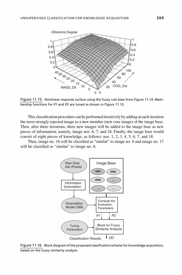
This classification procedure can be performed iteratively by adding at each iteration

the most strongly rejected image as a new member (new core image) of the image base.

Then, after three iterations, three new images will be added to the image base as new

pieces of information, namely, image nos. 6, 7, and 18. Finally, the image base would

consist of eight pieces of knowledge, as follows: nos. 1, 2, 3, 4, 5, 6, 7, and 18.

Then, image no. 16 will be classified as “similar” to image no. 6 and image no. 17

will be classified as “similar” to image no. 6.

Raw Data Set (Pixels)

InformationGranulation

Compute theEvaluationParameters

Block for Fuzzy Similarity Analysis

GranulationModel (GM)

Image Base

Classification Results

TuningParameters

P1 P2

DD

GM1 GM2

GM3 ...

......

Figure 11.16. Block diagramof the proposed classification scheme for knowledge acquisition,

based on the fuzzy similarity analysis.

0

20

4060

80100

05

1015

2025

3035

40

00.2

0.4

0.6

0.8

1

0

0.2

0.4

0.6

0.8

1

COG_DstWAS2_Dif

Diference Degree

Figure 11.15. Nonlinear response surface using the fuzzy rule base from Figure 11.14. Mem-

bership functions for P1 and P2 are tuned as shown in Figure 11.13.

UNSUPERVISED CLASSIFICATION FOR KNOWLEDGE ACQUISITION 269

11.10 CONCLUSION

In this chapter a special unsupervised classification scheme for large data sets and images

is proposed, based on a two-input fuzzy rule-based similarity procedure. In order to

extract the inputs for this fuzzy procedure, two growing-type unsupervised learning

algorithms are presented and compared. They convert the original “raw” data set (the

RGB data set from the image) into the so-called granulation (compressed) model with a

smaller number of neurons.

18171615141312111098760

1

2

3

4

5

Classified as:

Unknown Test (New) Images

Figure 11.18. Classificationresultsof the remaining (new)13 imagesusing the imagebasewith

the first 5 Images. The accepted results are shown as large ball symbols.

18171615141312111098760.05

0.1

0.15

0.2

0.25

0.3

0.35

0.4

0.45

0.5 Difference DegreeDD

Unknown (Test, New) Images

ThresholdTh = 0.33

Accepted

Rejected

Figure 11.17. Computed difference degrees of the new images that are used for the classi-

fication decision (accepted—rejected) based on the predefined threshold Th¼0.33.


It is shown that the Grow2 algorithm has the advantage over the Grow1 algorithm

because it produces a granulationmodel with fewer neurons thanGrow1within the same

granulation quality AVmin. Both algorithms Grow1 and Grow2 are much faster in

computation time compared to the standard offline learning algorithm Fixed, which uses

the same predetermined number of neurons.

The two parameters used in the fuzzy decision procedure for similarity analysis are

extracted from the obtained granulation model as follows. The first parameter P1 is the

center-of-gravity distance COGD between a given pair of data sets (images), and

parameterP2 represents theweighted average size difference, computed in two versions,

namely WASD and WAS2D.

The performance of the proposed fuzzy decision procedure for similarity analysis is

demonstrated in a test example of 18 images. In addition, the same example is used for the

more general computation scheme for knowledge acquisition under the assumption that

the first 5 images are used as core images in the initial image base. The iterative process of

classification leads to adding 3 new core images to the image base. The proposed

procedure could be used as an evolving computation scheme for knowledge acquisition

from a large (or even unlimited) number of images or other data sets.

Further development of the above computation schemes is considered in the

following two directions. The first one is to establish a proper human-defined criterion

for optimizing the parameters of the fuzzy similarity procedure, in order to achievemore

plausible humanlike results from the similarity analysis and classification. The second

direction is to further refine the iterative (evolving) procedure for knowledge acquisition

in order for it to be successfully used for knowledge extraction from online processes and

data streams.

11.11 REFERENCES


Plenum Press, 1981.

2. Ch. M. Bishop, Neural Networks for Pattern Recognition. Oxford University Press, 2003.

3. W. Pedrycz, Knowledge-Based Clustering: From Data to Information Granules. Wiley-

Interscience, 2005, p. 316.

4. T. Kohonen, Self-Organizing Maps, 3rd ed. Springer Series in Information Sciences. Berlin:

Springer, 2001.

5. T.Martinetz, S. Berkovich, K. Schulten, “Neural-Gas Network for Vector Quantization and Its

Application to Time-Series Prediction,” IEEE Trans. Neural Networks, Vol. 4, No. 4, pp.

558–569, 1993.

6. Lei. Xu, A. Krzyzak, E. Oja, “Rival Penalized Competitive Learning for Clustering Analysis,

RBFNet andCurveDetection,” IEEETrans.NeuralNetworks,Vol. 4,No.4, pp. 636–649,1993.

7. S. C. Ahalt, A.K.Krishnamurty, P. Chen,D. E.Melton, “Competitive LearningAlgorithms for

Vector Quantization,” Neural Networks, Vol. 3, pp. 277–291, 1990.

8. G. Vachkov, “Growing Neural Models for Process Identification and Data Analysis,” Int. J.

InnovativeComputing, Information andControl, IJICIC, Vol. 2,No. 1, pp. 101–123, February

2006.

REFERENCES 271

9. G. Vachkov, “Classification of Machine Operations Based on Growing Neural Models and

Fuzzy Decision,” CD-ROM. Proc. 21st European Conf. on Modelling and Simulation, ECMS

2007, Prague, Czech Republic, June 4–6, 2007, pp. 68–73.

10. G. Vachkov, H. Ishihara, “Learning Algorithms for Compression and Evaluation of Infor-

mation from Large Data Sets,” CD-ROM. Proc. SICE Annual Conference 2007, Takamatsu,

Japan, September 17–20, 2007, pp. 1837–1844.

11. G. Vachkov, H. Ishihara, “On-Line Unsupervised Learning for Information Compression and

Similarity Analysis of Large Data Sets,” CD-ROM. Proc. 2007 IEEE Int. Conf. on Mecha-

tronics and Automation, ICMA 2007, Harbin, China, August 5–8, 2007, pp. 105–110.

12. G. Vachkov, “Classification of Images Based on Fuzzy Similarity Analysis,” CD-ROM. Proc.

5th Int. Symposium on Management Engineering, ISME 2008, Graduate School on Infor-

mation, Production and Systems,Waseda University, Hibikino, Kitakyushu City, Japan, paper

R09, March, 15–17, 2008, pp. 162–169.

13. G. Vachkov, “Classification of Images Based on Information Granulation and Fuzzy Rule

Based Similarity Analysis,” CD-ROM. Proc. 2008 World Congress on Computational

Intelligence, WCCI 2008, FUZZ-IEEE 2008, Hong Kong, China, paper FS0528, June 1–6,

2008, pp. 2326–2332.


12AN EXTENDED VERSION OF THE

GUSTAFSON-KESSELALGORITHM FOR EVOLVINGDATA STREAM CLUSTERING

Dimitar Filev, Olga Georgieva

Abstract: The chapter deals with a recursive clustering algorithm that enables a real-

time partitioning of data streams. The proposed algorithm incorporates the advantages of

the Gustafson-Kessel clustering algorithm of identifying clusters with different shape

and orientation while expanding its area of application to the challenging problem of

real-time data clustering. The algorithm is applicable to a wide range of practical

evolving system–type applications, such as diagnostics and prognostics, system iden-

tification, real-time classification, and process quality monitoring and control.

12.1 INTRODUCTION

Cluster analysis is one of the challenging theoretical and practical problems in data

mining, signal processing, diagnostics and prognostics, and information retrieval in

numerous other application areas. Most of the clustering methods are based on the

concept of batch clustering; that is, the data set is assumed to be available before the

clustering analysis is carried out. In a wide range of applications, however, the data is

presented to the clustering algorithm in real time.

Recently, we have obseyrved a growing interest toward methods for real-time

clustering streams of data [7, 18, 19]. Among them are the methods for single-pass


and Nikola Kasabov


clustering, for example, [15, 21, 23], comprising techniques that find clusters by

executing one pass through the data set, in contrast to the iterative strategies like

K-means clustering. A prototypical representative of the one-pass evolving algorithms is

the evolving clustering method (ECM) [19]. It is a distance-based clustering method

where the cluster centers are represented by evolving nodes that are continuously

updated through changing their centers’ positions and adjusting their cluster radii.

Alternatively, new clusters are created.

The approach of single-pass clustering is also applied in the dynamic data

assigning algorithm (DDAA) [13]. It is a heuristic clustering method that detects a

single (good) cluster among noisy data, applying the concept of noise clustering [8, 9].

The aim is to discover an interesting pattern in terms of a specific group that might

cover only a small proportion of the full data set, rather than to partition the whole data

set into clusters. The evolving version of the algorithm [13, 14] is suitable for dealing

with data streams. It assigns every new data point to an already-determined good

cluster or alternatively to the noise cluster. The assignment can be done in a crisp or

fuzzy sense.

Alternative clustering algorithms, for example, DBSCAN [10] or its incremen-

tal version [11], take noise into account as well. DBSCAN defines clusters in terms

of a homogeneous minimum density; that is, the user must specify two para-

meters Eps and MinPts. For each point in a cluster, the Eps-neighborhood must

contain at least MinPts points; otherwise, the point is considered to be noise. This

means that the definition of noise is homogeneous in the whole data space, and the

decision as to whether points are to be marked as noise or as outliers strongly

depends on the setting of these parameters. The algorithm is applicable to image

analysis.

Some of the clustering methods are widely used as a foundation for structure

identification of fuzzy rule-based models [3, 6, 22]. Examples of clustering algorithms

that are used in model identification procedures include the mountain clustering

algorithm [22] and its modification—the subtractive clustering algorithm [6]. The

online extension of mountain/subtractive clustering utilizes recursive and noniterative

techniques for calculating the potential of the new data point in order to update

the existing clusters or to discover new ones [1, 2]. The method is targeted to real-

time modeling and classification tasks.

A newmethodology for dynamic data mining based on fuzzy clustering is proposed

in [7]. It continuously updates the structure and parameters of a fuzzy classifier by

incorporating a Fuzzy-C-Means (FCM) clustering algorithm [4].

In a number of real problems, such as performance analysis of dynamic systems,

and time-series data, as well as some forecasting and modeling tasks, the identified

clusters are not spherical as they are presumed to be by the commonly used FCM

clustering method and its derivatives, but are characterized with a different shape and

orientation in the space. Several clustering algorithms extend the original FCMmethod

to the case of clusters with a general shape [3, 12, 17, 20]. The Gustafson-Kessel (GK)

clustering algorithm [16] is commonly used in most of the cases as a powerful

clustering technique with numerous applications in various domains, including image

274 AN EXTENDED VERSION OF THE GUSTAFSON-KESSEL ALGORITHM

processing, classification, and system identification. By contrast to the FCMalgorithm,

its main feature is the local adaptation of the distance metric to the shape of the cluster

by estimating the cluster covariance matrix and adapting the distance-inducing matrix.

In addition, it is relatively insensitive to the data scaling and initialization of the

partition matrix.

In this chapter, we propose a new clustering algorithm called the evolving GK-

like (eGKL) algorithm that builds on the advantages of the GK algorithm as a

valuable clustering technique that is able to identify clusters with a generic shape

and orientation. We discuss the idea of expanding the original GK algorithm to the

problem of clustering data streams. We also address the issues of estimation of

the number of clusters and recursive updating and adaptation of their parameters to

the data.

The chapter is organized as follows. The second section presents the necessary

background on cluster analysis based on the GK algorithm. The idea of the evolving GK-

like algorithm and a simplified version are presented in the third section. The further

necessary methodological and computational considerations related to the evolving GK

concept are presented in the fourth and fifth sections, respectively. The evolving GK-like

algorithm is developed in the sixth section. Final conclusions are provided in the seventh

section.

12.2 CLUSTER ANALYSIS BY GK ALGORITHM

Objective function-based clustering aims at minimization of an objective function J that

represents the fitting error of the clusters with respect to the data. In this objective

function, the number of clusters has to be fixed in advance. The underlying objective

function for most of the clustering algorithms is [4]:

JðV ;U;FÞ ¼Xci¼ 1

XNk¼ 1

ðuikÞmd2ik ð12:1Þ

whereN is thenumberofdatapoints,c is thenumberofclustersgiveninadvance,uikanddikdenote correspondingly the membership degree and distance between the kth data point

xk ¼ ½xk1; xk2; . . . ; xkn�,k ¼ 1; . . . ;N and the ith cluster prototype, i ¼ 1; . . . ; c, andnis the number of features describing each data point.U ¼ fuikg is cN partitionmatrix.

In the simplest case, the cluster prototype is a single vector called, a cluster center, which

for the ith cluster is vi ¼ ½vi1; vi2; . . . ; vin�; V ¼ fvig is c n prototype matrix. The

fuzzifier m 2 ½1;¥Þ is the weighted exponent coefficient that determines how much

clusters may overlap. In most of cases, satisfactory results are obtained at m ¼ 2.

The distance dik used by the GK algorithm is a squared inner-product distance norm

that depends on a positive definite symmetric matrix Ai as follows:

d2ik ¼ xk�vik k2Ai

¼ ðxk�viÞAiðxk�viÞT ð12:2Þ

CLUSTER ANALYSIS BY GK ALGORITHM 275

The matrix Ai, i ¼ 1; . . . ; c determines the shape and orientation of the selected

cluster. Thus, the GK algorithm employs an adaptive distance norm unique for every

cluster as the norm-inducing matrix Ai is calculated by estimates of the data covariance:

Ai ¼ ½ridetðFiÞ�1=nF�1i ð12:3Þ

where ri is the cluster volume of the ith cluster and Fi is the fuzzy covariance matrix

calculated as follows:

Fi ¼PN

k¼ 1 ðuikÞmðxk�viÞTðxk�viÞPNk¼ 1 ðuikÞm

ð12:4Þ

Without any prior knowledge, the cluster volumes ri, i ¼ 1; . . . ; c are simply fixed

at one for each cluster.

Knowing the distances (12.2), the membership degree uik; i ¼ 1; . . . ; c,k ¼ 1; . . . ;N of each data to every cluster is calculated as a relative value:

uik ¼ 1Pcj¼ 1 ðdik=djkÞ2=ðm�1Þ

ð12:5Þ

and the cluster centers are defined as a weighted mean:

vi ¼PN

k¼ 1 ðuikÞmxkPNk¼ 1 ðuikÞm

ð12:6Þ

where m> 1 is a parameter defining the fuzziness of the clusters. In order to avoid the

trivial solution assigning no data to any cluster by setting all uik to zero, and to avoid

empty clusters, the following constraints are introduced:

uik 2 ½0; 1�; 1 � i � c; 1 � k � N ð12:7iÞXci¼ 1

uik ¼ 1; 1 � k � N ð12:7iiÞ

0 <XNi¼ 1

uik < N; 1 � i � c ð12:7iiiÞ

The GK algorithm, as do other FCM-based clustering algorithms, uses the Lagrange

multiplier method to minimize the cost functional (12.1). It iteratively determines the

membership degree uik and cluster parameters—cluster center vi and the fuzzy covari-

ance matrix Fi—which finally define the distance value dik. The optimization scheme of

the GK clustering is given in the appendix at the end of this chapter.

The obtained clusters are hyperellipsoids with arbitrary orientation. This general-

ized set of clusters well suits a variety of practical problems.


12.3 EVOLVING CLUSTERING BASEDONGK SIMILARITY DISTANCE

Although the GK algorithm possesses a great advantage over the other clustering

algorithms as it adapts the clusters according to their real shape, the algorithm is not

able to deal with streams of data and limits its scope to batch clustering due mainly to

three obstacles. These shortcomings have nothing to dowith the GK procedure itself but

with the attempt to expand all FCM-type clustering algorithms to cases that deal with

streaming data—a basic characteristic of an evolving-system-type application. First, it

processes only a fixed data set. Second, the algorithm assumes that the number of clusters

is known in advance. Finally, it determines the clusters by an iterative optimization

scheme. Thus, in practice, the new incoming data cannot be processed by the original

algorithm scheme as the stream of incoming data changes over time.

The idea of an alternative recursive clustering algorithm that is similar to the concept

of the GK algorithm in the sense of using clusters with general data structure is presented

in the following. Our solution is inspired by two of themost common recursive clustering

algorithms—the k-nearest neighbor (k-NN) [24] and the linear vector quantization

(LVQ) [25] algorithms.Wedo not consider the proposed algorithm an evolving version of

the GK algorithm but a rather recursive complement that uses the same Mahalanobis

distance—like metrics and the norm-inducing matrix—while avoiding the aforemen-

tioned drawbacks.

One simplified solution could be formulated according to the direct implementation

of the k-NN approach. Originally, we will be assuming that the GK has been applied to

identify an initial set of c clusters of the previously collected data. Each of those clusters

is defined by its center vi and fuzzy covariance matrix Fi. This assumption is realistic

given the fact that in almost all evolving applications some initial knowledge about the

data being processed is available.

We assume that the boundary of each cluster is defined by the cluster radius, which is

calculated from the membership degrees (12.5). The radius ri of the ith cluster is equal to

the maximal distance between the cluster center vi and the points belonging to this

cluster with membership degree larger than or equal to a given threshold membership

degree uh:

ri ¼ max vi�xj��

Ai

8xj2 ith cluster and uij>uh

ð12:8Þ

where �k kAiis the GK distance norm determined according to equation (12.2) and the

data xj belongs to the ith cluster with membership degree uij such that uij > uh.

Suppose xk is a new data point coming in currently. Three possibilities should be

evaluated. First, the data belongs to an existing cluster if it is within the cluster boundary.

This case imposes just clusters’ update. If the data point is not within the boundary of any

existing cluster, it may define a new cluster. Alternatively, xk could be an outlier, which

does not affect the data structure. These three possibilities for assigning xk are considered

in detail in the following.

The similarity between the new data point xk and each of the existing c clusters is

evaluated by checking theMahalanobis-like distances using equations (12.2) and (12.3),

EVOLVING CLUSTERING BASED ON GK SIMILARITY DISTANCE 277

dik ¼ffiffiffiffiffiffiffiffiffiffiffiffiffiffiffiffiffiffiffiffiffiffiffiffiffiffiffiffiffiffiffiffiffiffiffiffiffiffiffiffiffiffiffiffiffiffiffiffiffiffiffiffiffiffiffiffiffiffiffiffiffiffiffiffiffiffiffiðxk�viÞ½ðdetðFiÞÞ1=nF�1i �ðxk�viÞT

qð12:9Þ

and assuming that each cluster volume ri’s is fixed at one. The minimal distance dpkdetermines the closest cluster p as

p ¼ argmini¼ 1;...; c

ðdikÞ ð12:10Þ

The data point xk is assigned to the cluster p if the distance dpk is less than or equal to the

radius rp, that is, if the condition

dpk � rp ð12:11Þ

is satisfied. If this is the case, we can apply theKohonen rule [25] to update the pth cluster

parameters—cluster center and covariance matrix:

vp;new ¼ ð1�aÞvp;old þaxk ¼ vp;old þaðxk�vp;oldÞ ð12:12Þ

Fp;new ¼ ð1�aÞFp;old þaðxk�vp;oldÞTðxk�vp;oldÞ ¼¼ Fp;old þaððxk�vp;oldÞTðxk�vp;oldÞ�Fp;oldÞ

ð12:13Þ

where a ¼ [0.05 0.3] is a learning rate; vp,new and vp,old denote the new and old values of

the center; and Fp,new and Fp,old denote the new and old values of the covariance matrix.

If condition (12.11) fails, a new potential cluster is created and the number of clusters is

incremented:

c :¼ cþ 1 ð12:14Þ

Then, the incoming data xk is accepted as a center vnew of the new cluster,

vnew ¼ xk ð12:15Þ

and its covariance matrix Fnew is initialized with the covariance matrix of the closest

cluster:

Fnew ¼ Fp;old ð12:16Þ

In order to quantify the credibility of the estimated clusters, a parameter

Pi; i ¼ 1; . . . ; c is introduced to assess the number of points belonging to ith cluster.

Its lower bound is estimated from the minimal number of data points necessary to learn

the parameters of the covariance matrix. It is determined by the dimensionality n of the

data vector as:

Pmin ¼ nðnþ 1Þ=2 ð12:17Þ


Apparently, a high value of Pi not only guarantees the validity of the

covariance matrixes but improves the robustness of the algorithm with respect to

outliers. That is why we suggest a larger threshold Ptol, Ptol>Pmin that corresponds

to the desired minimal amount of points falling within the ri boundary of each cluster.

The threshold value is context determined due to the specificity of the considered data

set.

The simplified online GK-like clustering that summarizes the ideas presented above

is given in the following step-by-step description:

1. Initialization: Calculate the initial number of clusters c and the corresponding

matrixes V, U and Fi; i ¼ 1; . . . ; c by the offline GK algorithm. Choose in

advance: uh, a, Ptol.

Repeat for every new data point xk.

2. Calculate dik; i ¼ 1; . . . ; c:

dik ¼ffiffiffiffiffiffiffiffiffiffiffiffiffiffiffiffiffiffiffiffiffiffiffiffiffiffiffiffiffiffiffiffiffiffiffiffiffiffiffiffiffiffiffiffiffiffiffiffiffiffiffiffiffiffiffiffiffiffiffiffiffiffiffiffiffiffiffiðxk�viÞ½ðdetðFiÞÞ1=nF�1i �ðxk�viÞT

q

3. Determine the closest cluster p:

p ¼ argmini¼ 1;...; c

ðdikÞ

4. Calculate the radius rp of the closest cluster:

rp ¼ max vp�xj��

Ap

8xj2 pth cluster and upj>uh

5. If dpk � rp:

Update the center vp and matrix Fp:

vp,new = vp,old + a(xk�vp,old)

Fp,new = Fp,old + a ((xk�vp,old)T(xk�vp,old)�Fp,old)

Recalculate the partition matrix U.

else dpk>rp

Create a new cluster: vc+1 := xs; Fc+1 := Fp

Calculate the number Pc+1.

If Pc+1�Ptol

Accept the new cluster, c:= c+1.

else

Refuse the new cluster and keep the old structure.

end

end


The choice of the parameters uh, a, and Ptol is of real importance for the clustering

results. Themembership threshold uh is difficult to determine in advance and depends on

the density of the data set and the level of cluster overlapping. The default value of uh is

0.5, but being stricter in the identification of proper clusters the prescribed threshold

membership degree should be chosen larger. For a more tolerant identification it should

be chosen smaller. The learning rate a determines the step of searching and, thus, a large

value guarantees sparsely selected clusters. However, in some cases the large step is not

preferred as it leads to large changes that could ignore a valuable cluster. It might be

beneficial to use two different thresholdmembership values as uh is used to determine the

cluster radius of the existing clusters and uh_new to calculate the radius of the newly

created cluster. If we set uh >uh_new, we give more freedom in the new cluster selection,

whereas we remain strict in the assessment of the points belonging to the existing

clusters.

The algorithm is validated in two examples based on an artificial data set and the

benchmark electroencephalography (EEG) data set [36].

12.3.1 Application of the Algorithm to an Artificial Data Set

The clustering capability of the simplified evolving GK-like clustering algorithm

is demonstrated on an artificial data set generated by an unvaried nonlinear

function [3]:

yk ¼ 10�4sinð0; 001 k2Þk3þ e ð12:18Þ

where e is normally distributed random noise. The dynamics simulated by this function

present a typical behavior of a certain nonlinear process. The generated data set is

organized in a 200 2 data matrix, whose first column is formed by the values of the

vector k ¼ ½1 : 0:5 : 100� and the second column by the corresponding values of the

vector yk.

The off-line GK algorithm with parameters m ¼ 2 and tol ¼ 0.01 was applied to

the first 100 data points in order to initialize the simplified evolving algorithm

(Figure 12.1a) while the remaining data was treated as a data stream. Due to the

lack of a priori information the default value of the threshold membership degree

uh ¼ 0.5 and a low boundary level of the learning rate a ¼ 0.05 were considered. The

parameter Ptol ¼ 10 was determined to guarantee robustness of the clusters. The third

cluster was created after the 33-th incoming data had been added. Simultaneously, the

second cluster center was updated (Figure 12.1b). After the creation of the forth

cluster (Figure 12.1c) the rest of the data only updated the previously identified data

structures (Figure 12.1d).

Results comparable to the batchGK clustering application are obtainedwhenwe are

strict in the assessment of the existing clusters as uh ¼ 0.95 but more free in the

evaluation of the newly created cluster as uh_new ¼ 0.8 (Figure 12.2). In both cases, five

valuable clusters are selected.


12.3.2 Application of the Algorithm to a Benchmark Data Set

Multiple electrode time-series EEG recordings of control and alcoholic subjects are

provided by UC Irvine Machine Learning Repository [36]. This data arises from a large

study to examine EEG correlation to genetic predisposition to alcoholism. It contains

measurements from 64 electrodes placed on the scalp sampled at 256Hz (3.9ms epoch)

for 1 second.

Notwithstanding the EEGdata set provides a large amount of data series, herewe are

interested in a single series as a subject of online partitioning. Initially, the first 100 points

are clustered by the batch GK algorithm in four clusters. For the rest of the data, the

evolving clustering is accomplished through a parameter set close to the default values as

uh ¼ 0.6 and a ¼ 0.05. The parameter Ptol ¼ 10 was context defined. As a result, five

new clusters are selected that fit the changes in the signal shape (Figure 12.3a).

Figure 12.1. Clustering results: dots aredata; squ"res are cluster centers; the circle is the current

data point: (a) initial clusters; (b) the third selected cluster at 33rd incoming data; (c) the fourth

cluster selected at 173rd data point. (d) The last cluster is slightly updated until the rest of the

data have been accumulated.


If we reduce the threshold Ptol to the minimal value Ptol ¼ Pmin ¼ 3 according to

equation (12.17), we are able to detect all peaks provided in the data series, obtaining in

total 18 clusters (Figure 12.3b).

The simulation results show that the developed evolving algorithm discovers

relatively well the changes in the data structure. However, in some cases the cluster

centers are not precisely defined and their shape and orientation are not correctly

determined (Figure 12.2). The simplified evolving reasoning does not provide a reliable

procedure for initiation and adjustment of the newfound cluster. In the next section, these

drawbacks are overcome by applying amore sophisticated concept inspired by the theory

of statistical process control (SPC) and the idea to account for older observations within

a moving window length.

Figure 12.3. Evolving clustering of EEG data.

Figure 12.2. Squares are cluster centers of the evolving algorithm and stars are the centers of

the batch GK algorithm application.


12.4 METHODOLOGICAL CONSIDERATIONS

Some additional methodological and computational considerations related to the

evolving GK-like (eGKL) concept that concern the definition of the clusters’ radii and

recursive updating of the cluster parameters will be addressed in the preliminaries.

The main challenge is the determination of the cluster radius. The objective

function-based clustering algorithms establish the radius based on data as the value of

the cost function (12.1) can be seen as a measure of the total variance of xk from vi.

However, this assumption is not acceptable for an evolving data set due to the growing

amount of points coming in as a stream. In the following we propose a new approach for

determining a generic cluster radius that can be applicable independently of the data.

This approach is inspired by statistical process control as a powerful methodology for

identifying variations in monitored output variables that are due to actual input changes

rather than process noise.

The main reason to seek to transfer some of the concepts and techniques from the

established SPC methodology to the (new) field of evolving clustering is the similarity

between the streams of data that are the result of the process monitoring and the data in

evolving clustering. In both cases, we dealwith data that is generated by a specific system

(e.g., device, machine, process), that is, governed by certain model of physical law

defining some similarity relationships between the data over time. In the evolving system

concept, the data has a temporal dimension that defines amechanism of ordering the data

points/samples. This type of data is different than the type of data considered in

conventional clustering, where the temporal dimension is missing and the data is

regarded as different objects.

The process variable y could be associated with its current mean yi� if the monitored

process is in statistical control; that is, the variable y is within the process control limits

that are usually set at yi� � 3syi according to the following condition:

y�y*i j < 3syi

ð12:19Þ

where yi� and syi are the process mean and standard deviation corresponding to the ith

particular process condition. When y exceeds the process control band (12.19), the

system is considered out of control.

In practice, the process control condition (12.19) defines a similarity relation as all

values of ywithin the process control band yi� � 3syi are considered similar and could be

represented by the mean yi�. This reasoning could be extended from the perspective of

considering a single-dimensional similarity relation clustering of the process variable y

into clusters with centers yi�’s and respective radii 3syi’s. If the process variable takes

values that are out of the process control limits (12.19), this is an indication of a

substantial variable change, which could be additionally indicated by a trend over time,

ormultiple points below or above themean.When the process is out of statistical control,

the process control parameters are recalculated, resulting in a new mean value yj� and

standard deviation syj (Figure 12.4).

The statistical process control condition for an n dimensional process variable

yk ¼ ½yk1; yk2; . . . ; ykn� is defined through the squaredMahalanobis distanceD between

METHODOLOGICAL CONSIDERATIONS 283

the current vector yk and the population mean [26, 27], where the population mean and

covariance are approximated by the sample mean y* and covariance S of the certain

process control condition:

D2 ¼ ðy�y*ÞS�1ðy�y*ÞT ð12:20Þwhere

y* ¼ 1

N

XNk¼ 1

yk ð12:21iÞ

S ¼ 1

N

XNk¼ 1

ðyk�y*ÞTðyk�y*Þ ð12:21iiÞ

The process vector yk is considered in statistical control when D2 is upper bounded

by the chi-square distribution, that is,

D2 < x2n;b ð12:22Þ

where x2n;b is the (1�b)th value of the chi-square distribution with n degrees of freedom

andb is the probability of a false alarm. Several low-dimensional values of the distribution

for the well-known�3s and�2s limits are given in Table 12.1. It could be seen that the

condition (12.22) covers the single-dimensional case (12.19) for the case of a single

process value n ¼ 1 [28].

The multidimensional process control condition (12.22) defines a relation of

similarity for all vectors yk that are within the (squared) radius x2n;b. The data points

within this region could be viewed as a cluster with center y� and shape defined by the

covariance matrix S. The vectors yk that are characterized with large values of the

T A B L E 12.1.

b

x2n;b 0.0027 0.0455

1 9 4

n 2 11.8290 6.1801

3 14.1563 8.0249

Figure 12.4. Process variable (a) and its SPC (Shewhart) chart (b).


distance D2 are far away from the center of the cluster y* and are less likely to belong to

that particular cluster.

The squared radius of the cluster is independent of the data as it is determined by the

chi-square distribution constant x2n;b that remains the same for a given probability b and

dimensionality n of the vector yk. The constant x2n;b defines themaximal distanceD2 for a

given probability threshold 1 –b. Beyond that distance, we reject the null hypothesis thatthe process is in control. Thus, vectors yk that fail condition (12.22) are considered not to

belong to the specific cluster.

The other challenge is to transfer the concepts of the SPC to the problem of evolving

GK-like clustering. Some additional specifications related to the application of the SPC

condition (12.22) to the evolving clustering features have to be given. In order to

calculate the radii of the eGKL clusters that are induced by the Mahalanobis-like

distance (12.2), we modify expression (12.22) by multiplying the left and right sides of

the inequality with the nonnegative (the covariance matrix S is always positive

semidefinite) constant (det(S))1/n:

ðy�y*ÞS�1ðy�y*ÞTðdetðSÞÞ1=n < x2n;bðdetðSÞÞ1=n ð12:23Þ

Therefore, for a given probability b and dimensionality n of the vectors yk, the radii

of theMahalanobis-like distance (12.2), the induced eGKL clusters are dependent on the

determinant of the covariance matrix:

R2 ¼ x2n;bðdetðSÞÞ1=n

and the similarity measure that is associated with the Mahalanobis-like distance

clusters is:

d2 < R2 ð12:24Þ

where

d2 ¼ ðy�y*ÞðdetðSÞÞ1=nS�1ðy�y*ÞT ð12:25Þ

From expression (12.23), it is easy to see that GK-like clusters are identical to the

clusters generated by the similaritymeasure (12.22). Therefore, we can use either (12.22)

or (12.24) to determine the clusters. In the next section, we will introduce the similarity

measure (12.22) as a criterion for deciding whether a data vector belongs to a cluster in

the process of creating the eGKL clusters. Further, we will employ the distance measure

(12.25) in order to calculate the degrees of membership of the individual data vectors

similarly to the GK clustering algorithm.

Nevertheless, condition (12.22) provides a natural and objective way to define the

cluster radii. Its application is connectedwith restrictions for a normal distribution. If this

assumption is not valid, the vectors yk can be wrongly associated with process control

situations or can be identified as outliers. Several authors, for example, Thissen et al. [29]

and Fraley and Raftery [31], have explored the idea of using the multivariate process

METHODOLOGICAL CONSIDERATIONS 285

control of modeling nonnormally distributed process control regions by combining

Gaussian mixture clusters. However, all these works have been focused on batch-type

application of the expectation-maximization (EM) clustering method to estimate

a mixture of Gaussian functions and could not be directly transferred to the streaming

data set. The other restriction is in the ability of the SPC condition (12.22) to detect

anomalies as this capacity is significantly reduced with increasing process dimension-

ality [27]. Third, the calculation of (12.22) is considered tedious and impractical since it

involves updating the covariance matrix and calculation of its inverse for every new

observation vector yk [30]. The last drawback could be compensated by a recursive

computational scheme.

12.5 RECURSIVE COMPUTATIONAL ASPECTS

Though conditions (12.22) and (12.24) guarantee that the cluster radii are reliably

identified, the problem with the correct and exact adjustment of the newfound cluster is

still open. Conventional distance definition (12.20) through the sample mean and

covariance matrix (12.21) is not convenient for real-time implementation since it

requires buffering of data and does not support recursive evaluation of the similarity

measure (12.22). On the other hand, experience shows (see section 12.3) that one-step

update does not provide exact results. In order to compensate for these shortcomings we

apply the exponentially weighted moving average (EWMA) procedure. The mean

value (12.21i) is replaced with its exponentially weighted moving average version:

y*new ¼ ð1�aÞy*old þayk ¼ y*old þaðyk�y*oldÞ ð12:26Þ

where the constant forgetting factor 0 � a � 1 controls the rate of updating the new

mean y*new by assigning a set of exponentially decreasing weights to the older observa-

tions y*old . Thus, for a constant a, expression (12.26) recursively generates a vector of

positive weights:

W ¼ ½ð1�aÞkað1�aÞk�1að1�aÞk�2 � � � a� ð12:27Þ

with a unit sum. The vectorW forms a weighted average–type aggregating operator with

exponentially decreasing weights that depend on a. The key question in EWMA

application is the memory depth (moving window length) of the aggregating operator.

It can be shown that the memory depth Ka is approximately reciprocal to the forgetting

factor Ka ¼ 1/a. The moving window length is calculated for indexes belonging to the

soft interval:

s 2 fk�Kaþ 1; k� ð12:28Þ

where the symbol {indicates a soft lower interval limit that includes values with lower

indexes than (k�Ka), which have relatively low contribution [32, 33]. For a variable


parameter a ¼ 1/k, expression (12.26) equals the recursive form of the arithmetic

mean in (12.21).

Analogously to the recursive calculation of the mean values, we can apply the

EWMA SPC chart to derive an alternative exponentially weighted recursive expression

for the covariance matrix S:

Snew ¼ ð1�aÞSold þaðyk�y*oldÞTðyk�y*oldÞ ð12:29Þ

where Sold and Snew are the old and updated versions of the covariance matrix S. It is

easy to see that expression (12.29) is a weighted form of the average-based conventional

covariance matrix (12.21ii). For a ¼ 1/k, the exponentially weighted covariance

matrix (12.29) is identical to the recursive form of the covariance matrix (12.21ii).

However, the recursive calculations of the covariance matrix have to tackle another

problem as well. Although the recursive expression (12.29) significantly simplifies the

calculation of the covariance matrix, it does not resolve the problemwith the calculation

of its inversion. This problem is further complicated by the possible singularity of the

covariance matrix—a valid concern in cases of correlated data.

The algorithm for recursive calculation of the inverse covariance matrix follows

from the woodbury matrix inversion lemma [34]:

ðAþBCDÞ�1 ¼ A�1�A�1BðC�1þDA�1BÞ�1DA�1 ð12:30Þ

that is valid for any nonsingular squarematrixesA,C, and (C�1 þ DA�1B). If we denote

A ¼ ð1�aÞSold ; B ¼ dT ; C ¼ a; D ¼ d; d ¼ ðyk�y*oldÞ

we can obtain the recursive inversion of the covariance matrix (12.29) as follows:

S�1new ¼ ðð1�aÞSold þaðyk�y*oldÞTðyk�y*oldÞÞ�1

¼ ð1�aÞ�1S�1old�ð1�aÞ�1S�1old dTða�1þ dð1�aÞ�1S�1old dTÞ�1dð1�aÞ�1S�1old

¼ ð1�aÞ�1S�1old�G dð1�aÞ�1S�1old ¼ ðI�G dÞS�1oldð1�aÞ�1ð12:31Þ

where

G ¼ ð1�aÞ�1S�1old dTða�1þ dð1�aÞ�1S�1old dTÞ�1 ð12:32Þ

and S�1old and S�1new are the old and updated inverses of the covariance matrix S.

The nonsingularity requirements of the Woodbury matrix inversion lemma are

satisfied if S�1old is initialized as a diagonal matrix with sufficiently large elements and

0<a< 1.

By applying the determinant identity [35]:

detðAþ xyTÞ ¼ detðAÞð1þ yTA�1xÞ

RECURSIVE COMPUTATIONAL ASPECTS 287

wherex and y arevectorswith dimensionality equal to the rank of the squaredmatrixA, to

the expression for the updated covariance matrix (12.29):

detðSnewÞ ¼ detðð1�aÞSold þaðyk�y*oldÞTðyk�y*oldÞÞ

we can calculate the recursive version of the determinant of the covariance matrix. With

this aim, let us denote by detSnew and detSold the updated and the old values of the

covariance determinant, and also denote x ¼ aðyk�y*oldÞT ; y ¼ ðyk�y*oldÞT . A recur-

sive form of calculation of the determinant of the covariance matrix can be recursively

expressed as follows:

detSnew ¼ detðð1�aÞSold þaðyk�y*oldÞTðyk�y*oldÞÞ¼ detðð1�aÞSoldÞð1þaðyk�y*oldÞð1�aÞ�1S�1oldðyk�y*oldÞTÞ¼ ð1�aÞndetðSoldÞð1það1�aÞ�1ðyk�y*oldÞS�1oldðyk�y*oldÞTÞ¼ ð1�aÞn�1detSoldð1�aþaðyk�y*oldÞS�1oldðyk�y*oldÞTÞ ð12:33Þ

where S�1old is the old inverse of the covariance matrix S. Since the inverse covariance is

initialized as a diagonal matrix with sufficiently large elements, the initial value of the

determinant, detSold, of the initial covariance is easily obtained.

The previous equations show that covariance matrix (12.31) and its determi-

nant (12.33) could be easily recursively updated by using their previously estimated

values from the previous step. Both expressions will be further incorporated in the

formulation of the evolving GK-like algorithm.

12.6 EVOLVING GK-LIKE (eGKL) CLUSTERING ALGORITHM

If there isnoinitiallycollecteddataset,wecansupposethatvectorx1representsthefirstdata

point of thedata streamxk,k ¼ 1, 2,. . ..Weassociate thefirst cluster centerwith that point

v1 ¼ x1

and initialize its inverse covariance matrix and determinant, and the counter M1 of the

vectors belonging to the cluster:

F�11;new ¼ F�10 ; detF1;new ¼ detðF0Þ; M1 ¼ 1 ð12:34Þ

where F0 is an initial estimate of the covariance matrix. The initial covariance matrix

could be evaluated as an sample covariance of the already-collected data. If such

information does not exist, the matrix is initialized as a diagonal matrix F�10 ¼ gI,where I is an identity matrix of size n and g is a sufficiently large positive number. This

initialization corresponds to assigning a small ball-type cluster around the first cluster

center.


Suppose we have c cluster centers when the kth data vector is presented. The

similarity between xk and each of the existing c clusters is evaluated by checking the

similarity relation (i.e., the process control condition) (12.22):

D2ik < x2

n;b; i ¼ ½1; c� ð12:35Þ

where

D2ik ¼ ðxk�viÞF�1i ðxk�viÞT ð12:36Þ

Dik is the Mahalanobis distance of xk to each of the already-identified c cluster centers.

The minimal distance Dpk:

p ¼ arg mini¼ ½1;c�

ðDikÞ;D2ik < x2

n;b; i ¼ ½1; c� ð12:37Þ

determines the pth cluster that is closest to the kth data vector xk that simultaneously

satisfies condition (12.35). In this case the vector xk is assigned to the pth cluster, for

which we apply updating expressions (12.26), (12.31), (12.32), (12.33) to recalculate the

pth cluster’s characteristics—cluster center, inverse covariance matrix, and its deter-

minant—as follows:

vp;new ¼ ð1�aÞvp;old þa xk ¼ vp;old þaðxk�vp;oldÞ ð12:38Þ

F�1p;new ¼ ðI�Gpðxk�vp;oldÞÞF�1p;old

1

1�a ð12:39Þ

where

Gp ¼ F�1p;oldðxk�vp;oldÞTa

1�aþaðxk�vp;oldÞF�1p;oldðxk�vp;oldÞT

detFp;new ¼ ð1�aÞn�1detFp;oldð1�aþaðxk�vp;oldÞF�1p;oldðxk�vp;oldÞTÞð12:40Þ

As the parameter Mp counts the number of data points that fall within the boundary of

each cluster, its value is increased by assigning a point to the closest cluster:

Mp;new ¼ Mp;old þ 1 ð12:41Þ

Simultaneously, we update in the opposite direction the remaining cluster centers in an

attempt to move them away from the pth cluster:

vq;new ¼ vq;old�aðxk�vq;oldÞ; q ¼ ½1; c�; q 6¼ p ð12:42Þ

The parameterMi, i ¼ [1,c] assesses the credibility of the estimated clusters. Its minimal

value corresponds to theminimal number of data points needed to learn the parameters of

EVOLVING GK-LIKE (eGKL) CLUSTERING ALGORITHM 289

the ith inverse covariancematrixF�1i that is estimated by the dimensionality n of the data

vector:

Mmin ¼ nðnþ 1Þ=2

However, from a practical point of view, the algorithm needs a more conservative

value of the Mmin parameter to ensure the cluster significance:

Mmin ¼ Q nðnþ 1Þ=2where Q is a credibility parameter with default value Q ¼ 2. A high value of Mmin not

only guarantees the validity of covariance matrixes Fi’s but improves the robustness of

the algorithm with respect to outliers.

In the opposite case, condition (12.35) fails. The vector xk is not similar to any of the

cluster centers and it could not be assigned to any of the existing clusters. So, the natural

decision is to create a new cluster. However, before implementing that step we check

whether that fact is not due to the lack of credible clusters surroundingxk, that is, whether

the condition:

Mp0 < Mmin ð12:43Þwhere

p0 ¼ arg mini¼ ½1;c�

ðDikÞ

applies. If this is the case, we have to fulfill the updates (12.38)–(12.42) to the closest

cluster p0. Note that for cluster p0 the similarity condition is not satisfied.Otherwise, a new

cluster is created and the number of clusters is incremented:

cnew ¼ cold þ 1

The center of the new cluster is initializedwith the newdata pointxk. The covariance

matrix of the newly formed cluster is initialized with the sample covariance matrix of the

population:

vc;new ¼ xk; F�1c;new ¼ F�10 ; detFc;new ¼ detðF0Þ; Mc;new ¼ 1 ð12:44Þ

As the parameter Mi accounts for the number of points that form a given cluster, it

could be used to control the value of the learning rate a. The inequality Mi<Mmin

presents a situationwhen the estimated ith cluster is sparse and its covariancematrixFi is

not completely estimated. Obviously, we should not allow for any forgetting of the data,

and the true sample inverse covariance is calculated by considering:

a ¼ 1=ðMminþ 1ÞFor dense clusters that contain points exceeding the minimal number of Mmin, we

consider a learning rate

_a � 1

_=Mmin ð12:45Þ


that guarantees that the memory depth (the length of themoving window)will not be less

than the minimumMmin. This ensures credible estimation of the inverse covariance and

also that the clusters will be continually updated with new data.

The clusters defined by the similarity relationship (12.35) can be viewed as sets of

points that are characterized with their sample means, covariance matrices, and radii

x2n;b.We can extend those clusters by assigning additional data points that belong to them

with degrees of fuzzy membership corresponding to their similarities to the identified

cluster centers. We can use either the Mahalanobis distance (12.36) or the Mahalanobis-

like distance as in the original GK algorithm:

d2ik ¼ ðxs�viÞ½ðdetðFiÞÞ1=nF�1i �ðxs�viÞT i ¼ ½1; c� ð12:46Þ

to determine themembership grades of all points to each core cluster. In the first case, we

get degrees of membership that are calculated from the distances Dik’s by (12.36):

Uik ¼ 1Pcj¼ 1 ðDik=DjkÞ2

; 8i;Mi > Mmin; i ¼ 1; c½ � ð12:47Þ

or alternatively, if the Mahalanobis-like distances dik’s from expression (12.46) are

determined, another set of membership functions could be calculated:

uik ¼ 1Pcj¼ 1 ðdik=djkÞ2

; 8i;Mi > Mmin; i ¼ 1; c½ � ð12:48Þ

For every vector xk, the memberships of any of the credible clusters yield a set

of membership functions that is similar to the one used in the GK clustering

algorithm. We’ll call the clusters with membership functions according to (12.48)

the eGKL clusters because of their similarity to the ones used in the GK clustering

algorithm.

Next we summarize the eGKL algorithm. We assume no prerequisite information

about the clusters.

Summary of the eGKL Algorithm

1. Choose the probability of a false alarm b and define the x2n;b according to

Table 12.2. We consider a default probability of false alarm b ¼ 0.0455 that

relates to the 2s process control band in the single-variable SPC. Estimated

values of x2n;b for different sizes of the data vector x are given in Table 12.1:

T A B L E 12.2.

n 2 3 4 5 6 7 8 9 10

x2n;0:0455 6.1801 8.0249 9.7156 11.3139 12.8489 14.3371 15.7891 17.2118 18.6104


2. Choose the initialization parameter g for the inverse covariance matrix (we

consider default values g ¼ 50):

F�10 ¼ gI

3. Choose the cluster credibility parameter Q (default value Q ¼ 2) and

establish Mmin:

Mmin ¼ Q nðnþ 1Þ=2

4. Read the first data point x1 and set c ¼ 1.

5. Initialize the first cluster as follows:

vc ¼ x1; F�1c;new ¼ F�10 ; det Fc;new ¼ detðF0Þ; Mc ¼ 1

6. Read the next data point xk..

7. Calculate the membership of xk in all credible clusters:

uik ¼ 1Pcj¼ 1 ðdik=djkÞ2

; 8i;Mi > Mmin; i ¼ 1; c½ �

where

d2ik ¼ ðxk�viÞ½ðdetðFiÞÞ1=nF�1i �ðxk�viÞT < R2; i ¼ ½1; c�

8. Check the similarity of xk to the existing clusters:

D2ik < x2

n;b; i ¼ ½1; c�

where

D2ik ¼ ðxk�viÞF�1i ðxk�viÞT

9. Identify the closest cluster:

p ¼ arg mini¼ ½1;c�

ðDikÞ

10. If D2pk < x2

n;b or Mp<Mmin, then do the following:

10.1. Update the parameters of the pth cluster:

vp;new ¼ vp;old þaðxk�vp;oldÞ

F�1p;new ¼ ðI�Gpðxk�vp;oldÞÞF�1p;old

1

1�a


where

Gp ¼ F�1p;oldðxk�vp;oldÞTa

1�aþaðxk�vp;oldÞF�1p;oldðxk�vp;oldÞT

detFp;new ¼ ð1�aÞn�1detFp;oldð1�aþaðxk�vp;oldÞF�1p;oldðxk�vp;oldÞTÞMp;new ¼ Mp;old þ 1

10.2. Move away the centers of remaining clusters:

vq;new :¼ vq;old�aðxk�vq;oldÞ; q ¼ ½1; c�; q 6¼ p

10.3. Go to step 6.

11. If none of the conditions D2pk < x2

n;b or Mp<Mmin applies, then do the

following:

11.1. Increment c.

11.2. Initialize the next cluster as follows:

vc ¼ xk; F�1c;new ¼ F�10 ; detFc;new ¼ detðF0Þ; Mc ¼ 1;

11.3. Go to step 6.

Without a loss of generality, the eGKL algorithm could be applied if a set of clusters

has been already identified with the conventional batch GK algorithm. In this case, the

algorithm starts from step 6.

The application of the eGKL algorithm to the problem of real-time clustering

streams of data is illustrated in the example data set generated by (12.18). However, the

data stream data set was extended to 994 data points. This new data set shows a large

difference in the magnitude of the elements of the two-dimensional row data vectors. In

order to ensure that the two data vectors arewithin the samemagnitude in their variations

independently of the different physical meanings, the raw vectors y’s are replaced by

their standardized values

Yk ¼ ðyk�y*ÞðdiagðsÞÞ�0:5

where y� and s are the sample mean and covariance matrix. This preprocessing

standardization is a realistic assumption that can be easily implemented as a process of

recursive learning of the means and the variances of the components of the raw data x:

y*k ¼k�1k

y*k�1þ1

kyk; y

*1 ¼ 0

s2k ¼k�1k

s2k�1þ1

k�1 diagððyk�y*kÞTðyk�y*kÞÞ; s21 ¼ 0


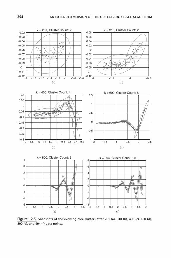
-2 -1.8 -1.6 -1.4 -1.2 -1 -0.8 -0.6-0.12

-0.11

-0.1

-0.09

-0.08

-0.07

-0.06

-0.05

-0.04

-0.03

-0.02k = 201, Cluster Count: 2

-2 -1.5 -1 -0.5-0.12

-0.1

-0.08

-0.06

-0.04

-0.02

0

0.02

0.04

0.06

0.08k = 310, Cluster Count: 2

(b)(a)

-2 -1.8 -1.6 -1.4 -1.2 -1 -0.8 -0.6 -0.4 -0.2-0.3

-0.25

-0.2

-0.15

-0.1

-0.05

0

0.05


-2 -1.5 -1 -0.5 0 0.5-1

-0.5

0

0.5

1


(d)(c)

-2 -1.5 -1 -0.5 0 0.5 1 1.5-3

-2

-1

0

1

2

3

4k = 800, Cluster Count: 8

-2 -1.5 -1 -0.5 0 0.5 1 1.5 2-6

-4

-2

0

2

4

6

8k = 994, Cluster Count: 10

(e) (f)

Figure 12.5. Snapshots of the evolving core clusters after 201 (a), 310 (b), 400 (c), 600 (d),

800 (e), and 994 (f) data points.


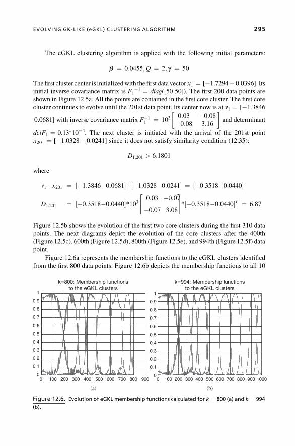
The eGKL clustering algorithm is applied with the following initial parameters:

b ¼ 0:0455;Q ¼ 2; g ¼ 50

Thefirst cluster center is initializedwith the first data vectorx1 ¼ [�1.7294� 0.0396]. Its

initial inverse covariance matrix is F1�1 ¼ diag([50 50]). The first 200 data points are

shown in Figure 12.5a. All the points are contained in the first core cluster. The first core

cluster continues to evolve until the 201st data point. Its center now is at v1 ¼ [�1.38460.0681] with inverse covariance matrix F�11 ¼ 103

0:03 �0:08�0:08 3:16

� �and determinant

detF1 ¼ 0.13�10�4. The next cluster is initiated with the arrival of the 201st point

x201 ¼ [�1.0328� 0.0241] since it does not satisfy similarity condition (12.35):

D1;201 > 6:1801

where

v1�x201 ¼ ½�1:3846�0:0681��½�1:0328�0:0241� ¼ ½�0:3518�0:0440�

D1;201 ¼ ½�0:3518�0:0440�*1030:03 �0:07�0:07 3:08

" #*½�0:3518�0:0440�T ¼ 6:87

Figure 12.5b shows the evolution of the first two core clusters during the first 310 data

points. The next diagrams depict the evolution of the core clusters after the 400th

(Figure 12.5c), 600th (Figure 12.5d), 800th (Figure 12.5e), and 994th (Figure 12.5f) data

point.

Figure 12.6a represents the membership functions to the eGKL clusters identified

from the first 800 data points. Figure 12.6b depicts the membership functions to all 10

0 100 200 300 400 500 600 700 800 9000

0.1

0.2

0.3

0.4

0.5

0.6

0.7

0.8

0.9

1

0

0.1

0.2

0.3

0.4

0.5

0.6

0.7

0.8

0.9

1

k=800: Membership functionsto the eGKL clusters

0 100 200 300 400 500 600 700 800 900 1000

k=994: Membership functionsto the eGKL clusters

(b)(a)

Figure 12.6. Evolution of eGKL membership functions calculated for k ¼ 800 (a) and k ¼ 994

(b).


clusters identified from that data stream. Membership functions are calculated using the

Mahalanobis-like distance.

12.7 CONCLUSION

This chapter presents one approach to the challenging problem of discovering

structures of streaming data in real time. The proposed evolving Gustafson-Kessel-

like (eGKL) clustering algorithm is a step toward the problem of online evolving

clustering of streams of data. Although inspired by the generic cluster shape and

orientation of the Gustafson-Kessel algorithm, the new algorithm is closer to the spirit

of the k-NN and LVQ clusteringmethods. It provides amethodology for adaptive, step-

by-step identification of clusters that are similar to the GK clusters. The algorithm is

based on a new approach to the problem of estimation of the number of clusters and

their boundaries that is motivated by the identified similarities between the concept of

evolving clustering and the well-established multivariate SPC techniques. The pro-

posed algorithm addresses some of the basic problems of the new field of evolving

systems, for example, recursive estimation of the cluster centers, inverse covariance

matrixes, covariance determinants,Mahalanobis distance-type similarity relations that

are enablers for computationally efficient implementation in real-time identification,

classification, prognostics, process modeling, and anomaly detection, and other

embedded-system types of applications.

Appendix: GK Algorithm

Initialization: Choose in advance the number of clusters c, theweight exponentm(default m ¼ 2), and the termination tolerance tol (default tol ¼ 0,01) andvolumes ri (default ri ¼ 1, i ¼ 1, . . ., c).

1. Initialize randomly partition matrix UðoÞ according to the membership constrains.

Repeat forl ¼ 1, 2, . . ..2. Compute the cluster centers:

vðlÞi ¼

PNk¼ 1 ðuðl�1Þik ÞmxkPNk¼ 1 ðuðl�1Þik Þm

; for i ¼ 1; . . . ; c

3. Compute the cluster covariance matrixes:

Fi ¼PN

k¼ 1 ðuðl�1Þik Þmðxk�vðlÞi ÞTðxk�vðlÞi ÞPNk¼ 1 ðuðl�1Þik Þm

; for i ¼ 1; . . . ; c

4. Compute the distances between the current point xk and the cluster centers vi:

d2ik ¼ ðxk�vðlÞi Þ½ðridetðFiÞÞ1=n F�1i �ðxk�vðlÞi ÞT ; i ¼ 1; . . . ; c ; k ¼ 1; . . . ;N


5. Update the partition matrix:

If dik > 0 for i ¼ 1; . . . ; c k ¼ 1; . . . ;N

uðlÞik ¼

1Pcj¼ 1 ðdik=djkÞ2=ðm�1Þ

otherwise uðlÞik ¼ 0 if dv > 0; and u

ðlÞik 2 ½0; 1�with

Xci¼ 1

uðlÞik ¼ 1:

until UðlÞ�Uðl�1Þ�� < tol.

12.8 ACKNOWLEDGMENTS

The research of the second author was partly supported by the project “SISTER:

Strengthening the IST Research Capacity of Sofia University” of 7FP-PEGPOT-

2007-1 program of the European Union.

12.9 REFERENCES

1. P. P. Angelov, Evolving Rule-Based Models: A Tool for Design of Flexible Adaptive Systems.

Heidelberg, Germany: Springer-Verlag, 2002.

2. P. P. Angelov, D. P. Filev, “An Approach to Online Identification of Takagi-Sugeno Fuzzy

Models,” IEEE Trans. on SMC—Part B: Cybernetics, Vol. 34, No. 1, pp. 484–498, 2004.



Plenum Press, 1981.

5. J. C. Bezdek, “A Convergence Theorem for the Fuzzy ISODATA Clustering Algorithms,”

IEEE Trans. Pattern Analysis and Machine Intelligence, Vol. 2, pp. 1–8, 1980.

6. S. L.Chiu, “FuzzyModel IdentificationBased onCluster Estimation,” J. Intelligent andFuzzy

Systems, Vol. 2, pp. 267–278, 1994.

7. F. Crespo, R.Weber, “AMethodology for Dynamic DataMining Based on Fuzzy Clustering,”

Fuzzy Sets and Systems, Vol. 150 pp. 267–284, 2005.

8. R. H. Dav�e, “Characterization and Detection of Noise in Clustering,” Pattern Recognition

Letters, Vol. 12, pp. 657–664, 1991.

9. R. H. Dav�e, R. Krishnapuram, “Robust ClusteringMethods: AUnified View,” IEEE Trans. on

Fuzzy Systems, Vol. 5 pp. 270–293, 1997.

10. M. Ester, H.-P. Kriegel, J. Sander, X. Xu, “A Density-Based Algorithm for Discovering

Clusters in LargeSpatial DatabaseswithNoise.”Proc. 2nd Int. Conf. onKnowledgeDiscovery

and Data Mining, Portland, OR, 1996, pp. 226–231.

11. M. Ester, H.-P. Kriegel, J. Sander,M.Wimmer, X.Xu, “Incremental Clustering forMining in a

Data Warehousing Environment.” Proc. 24th Int. Conf. Very Large Databases, VLDB, 1998,

pp. 323–333.

REFERENCES 297

12. I. Gath, A. B. Geva, “Unsupervised Optimal Fuzzy Clustering,” IEEE Trans. on Pattern

Analysis and Machine Intelligence, Vol. 7, pp. 773–781, 1989.

13. O. Georgieva, F. Klawonn,“Dynamic Data Assigning Assessment Clustering of

Streaming Data, Applied Soft Computing—Special Issue on Dynamic Data Mining (in

press), 2008.

14. O. Georgieva, F. Klawonn, “EvolvingClustering via theDynamicDataAssigningAssessment

Algorithm.” Proc. 2006 International Symposium on Evolving Fuzzy Systems, Ambleside,

UK, September 7–9, 2006, pp. 95–100, IEEE Catalog Number: 06EX1440; ISBN: 0-7803-

9718-5.

15. C. Gupta, R. L. Grossman, “GenIc: A Single Pass Generalized Incremental Algorithm for

Clustering.” 2004 SIAM Int. Conf. on Data Mining, SDM 04 (SIAM), Philadelphia, 2004, pp.

137–153.

16. D. E. Gustafson, W. C. Kessel, “Fuzzy Clustering with a Fuzzy Covariance Matrix.” Proc.

IEEE CDC (IEEE), San Diego, 1979, pp. 761–766.

17. F. H€oppner, F. Klawonn, R. Kruse, T. Runkler, Fuzzy Cluster Analysis. Chichester, NewYork:

John Wiley & Sons, 1999.

18. G. Hulten, L, Spencer, P. Domingos, “Mining Time-Changing Data Streams.” Proc. of KDD

2001. New York: ACM Press, 2001, 97–106.

19. N. K.Kasabov, Q. Song, “DENFIS: Dynamic EvolvingNeuro-Fuzzy Inference System and Its

Application for Time-Series Prediction,” IEEE Trans. Fuzzy Systems, Vol. 10, pp. 144–154,

2002.

20. A. Keller, F. Klawonn, “Adaptation of Cluster Sizes in Objective Function Based Fuzzy

Clustering.” Intelligent Systems: Technology and Applications, Vol. IV: Database and

Learning Systems ( C. T. Leondes,ed.) Boca Raton: CRC Press, 2003, pp. 181–199.

21. R. Papka, J. Allan, “On-Line New Event Detection Using Single Pass Clustering,” UMASS

Computer Science Technical Report 98-21, 1998.

22. R. Yager, D. Filev, Essentials of Fuzzy Modeling and Control. NewYork: JohnWiley& Sons,

1994.

23. J. Yang, “Dynamic Clustering of Evolving Streams with a Single Pass.” Proc. 19th Int. Conf.

on Data Engineering, ICDE’03, Bangalore, 2003, pp. 695–697.

24. J. Keller, M. Gray, J. Givens, “A Fuzzy k-Nearest Neighbor Algorithm,” IEEE Trans. on

Systems, Man, and Cybernetics, Vol. 15, pp. 580–585.

25. T. Kohonen, Self-Organization and Associative Memory, 3rd ed. Berlin: Springer-Verlag.

26. T. Ryan, Statistical Methods for Quality Improvement. New York: JohnWiley & Sons, 1989.

27. N. Ye, C. Borror, D. Parmar, “Scalable Chi-Square Distance versus Conventional Statistical

Distance for Process Monitoring with Uncorrelated Data Variables,” Quality and Reliability

Engineering International, Vol. 19, pp. 505–515.

28. N. Ye, Q. Chen, S. M. Emran, S. Vilbert, “ Hotelling’sT2 Multivariate Profiling for Anomaly

Detection.” Proc. 1st IEEE SMC Inform. Assurance and Security Workshop, 2000.

29. U. Thissen et al., “Multivariate Statistical Process Control Using Mixture Modeling,” J.

Chemometrics, Vol. 19, pp. 23–31, 2005.

30. N. Ye et al., “Probabilistic Techniques for Intrusion Detection Based on Computer Audit

Data,” IEEE Trans. on Systems, Man and Cybernetics, Part A, Vol. 31, pp. 266–274, 2001.

31. C. Fraley, A. Raftery, “Model-Based Clustering, Discriminant Analysis, and Density

Estimation,” J. Am. Statist. Assoc., Vol. 97, pp. 611–631, 2002.


32. A. Beex, J. Zeidler, “Non-Wiener Effects in Recursive Least Squares Adaptation,” Proc. 7th

Int. Symposium on Signal Processing and Its Applications, Vol. 2, 2003, pp. 595–598.

33. D. Erdogmus et al., “Recursive Principal Components Analysis Using Eigenvector Matrix

Perturbation,” EURASIP J. Applied Signal Processing, Vol. 13, pp. 2034–2041, 2004.

34. M. Woodbury, “Inverting Modified Matrices: Memorandum Rept. 42,”Statistical Research

Group, Princeton University, Princeton, NJ, p. 4, 1950.

35. M. Brookes, The Matrix Reference Manual. London: Imperial College, 2005.

36. UC Irvine Machine Learning Repository, http://archive.ics.uci.edu/ml/databases/eeg/eeg.

data.html.

REFERENCES 299

13

EVOLVING FUZZYCLASSIFICATION OF

NONSTATIONARY TIME SERIESYe. Bodyanskiy, Ye. Gorshkov, I. Kokshenev, V. Kolodyazhniy

Abstract:The problem of adaptive segmentation of time series changing their properties

at a priori unknown moments is considered. The proposed approach is based on the idea

of indirect sequence clustering, which is realized with a novel robust evolving recursive

fuzzy clustering algorithm that can process incoming observations online (possibly in

real-time mode) and is stable with respect to outliers that are often present in real data.

An application to the segmentation of a biological time series confirms the efficiency of

the proposed algorithm.

13.1 INTRODUCTION

Recent years have witnessed a growing interest in the analysis of nonstationary time

series changing their properties at a priori unknown moments. The problems of time-

series analysis are quite typical in speech processing, text and web mining, robot sensor

analysis, and especially in medical and biological diagnostics. It is important to note that

these problems often need to be solved online as new data become available.

In the process of solving such problems, the time series is partitioned (segmented)

into internally homogeneous (homomorphic) parts, which are subsequently represented

via some more compact description for further diagnosis.


and Nikola Kasabov


Such problems in some cases were solved using the approach based on the methods

of properties change detection in signals and systems [1]. However, the known algo-

rithms are usually oriented to the detection of abrupt changes, and are not well suited for

the detection of slow variations in characteristics.

In real situations, especially in biomedical applications, internal changes in the

monitored object are usually quite slow, and the stable states of an organism usually

overlap in many of their characteristics. Besides that, transient states exist that simul-

taneously have characteristics of several stable ones.

In this situation, themethods of fuzzy clustering of time series are preferable because

of the ability to find parameters of the overlapping clusters or segments. They are based

on thewidely used techniques of fuzzy cluster analysis [2–4]. Thesemethods have proved

to be effective in solving many problems in batch mode, but their use in real time is

complicated by a number of difficulties. One can overcome some of these difficulties

using the fast evolvingmethods of recursive cluster analysis [5–9].However, themethods

mentioned earlier are capable of efficient data clustering when the clusters are over-

lapping only with the assumption that the clusters are compact, that is, they do not have

abrupt (anomalous) outliers. Whereas real data sets usually contain up to 20% out-

liers [10–12], the assumptionof cluster compactnessmay sometimes become inadequate.

Thus, the problem of cluster analysis of data with heavy-tailed distributions has

receivedmore andmore attention in recent years. Variousmodifications of the clustering

methods mentioned earlier were proposed in papers [13–15] to process data containing

outliers.

At the same time, most of the proposed robust fuzzy clustering algorithms are not

suitable for real-time or sequential operation. So, it is advisable to develop recursive

algorithms for robust fuzzy clustering of time series, having evolving properties and

suitable for the sequential processing of incoming data, when the characteristics of the

system generating the data are changing with time.

13.2 PREPROCESSING OF TIME SERIES AND INDIRECTSEQUENCE CLUSTERING

In the problems of segmentation of time series Y ¼ fyð1Þ; yð2Þ; . . . ; yðkÞ; . . . ; yðTÞg, theindirect sequence clustering approach [14] is used quite often. It consists in the extraction

of some characteristic features from the time series and their subsequent mapping onto

a transformed feature space, where known space-based clustering algorithms can be

used to form clusters. Such features can be the correlation, regression, and spectral

characteristics of the time series, which in our case should be computed with adaptive

iterative procedures.

For this purpose, such estimates as mean, variance, and autocorrelation coefficients

can be used. To provide adaptive properties, these estimates can be computed via

exponential smoothing [1]. The mean value can be estimated as

SðkÞ ¼ a yðkÞþ ð1�aÞSðk�1Þ; 0 < a < 1 ð13:1Þwhere a ¼ 2=ðN þ 1Þ corresponds to smoothing on a moving window of width N.

302 EVOLVING FUZZY CLASSIFICATION OF NONSTATIONARY TIME SERIES

The variance of the time series can be estimated as

s2ðkÞ ¼ aðyðkÞ�SðkÞÞ2þð1�aÞs2ðk�1Þ ð13:2Þ

and the autocorrelation coefficients as

rðk; tÞ ¼ aðyðkÞ�SðkÞÞðyðk�tÞ�SðkÞÞþ ð1�aÞrðk�1; tÞ ð13:3Þ

where t ¼ 1; 2; . . . ; tmax.

Thus, a feature vector xðkÞ ¼ ðsðkÞ; s2ðkÞ; rðk; 1Þ; rðk; 2Þ; . . . ; rðk; tmaxÞÞT of

dimensionality 2þ tmax is computed at every instant k, such that a set ofG n-dimensional

feature vectors X ¼ fxð1Þ; xð2Þ; . . . ; xðTÞg is formed, where xðkÞ 2 Rn, k ¼ 1;2; . . . ; T . The output of a fuzzy clustering algorithm should be the separation of the

source data into m clusters with some degrees of membership wjðkÞ of the kth feature

vector xðkÞ to the jth cluster, where m in the common case is unknown and can change

over time.

In what follows, we make an attempt to derive an adaptive computationally simple

robust fuzzy clustering algorithm for recursive data processing in the online mode as

more and more data become available.

13.3 RECURSIVE FUZZY CLUSTERING APPROACH

The approach that we use belongs to the class of the objective function–based algo-

rithms [2] that are designed to solve the clustering problem via the optimization of

a certain predetermined clustering criterion, and are, in our opinion, the best grounded

from the mathematical point of view.

We consider the objective function

EðwjðkÞ; cjÞ ¼XTk¼1

Xmj¼1

wbj ðkÞDðxðkÞ; cjÞ ð13:4Þ

subject to constraints

Xmj¼1

wjðkÞ ¼ 1; k ¼ 1; . . . ; T ð13:5Þ

0 <XTk¼1

wjðkÞ � T ; j ¼ 1; . . . ;m ð13:6Þ

Here wjðkÞ 2 ½0; 1� is the degree of membership of the vector xðkÞ to the jth cluster, cj isthe prototype (center) of the jth cluster, b is a nonnegative parameter, referred to as

RECURSIVE FUZZY CLUSTERING APPROACH 303

a fuzzifier (usually b ¼ 2), and DðxðkÞ; cjÞ is the distance between xðkÞ and cj in the

adopted metrics. The result of the clustering is assumed to be a T m matrix

W ¼ fwjðkÞg, referred to as the fuzzy partition matrix.

Note that since the elements of the matrixW can be regarded as the probabilities of

the hypotheses of data vectors’ membership in certain clusters, the procedures generated

from (13.4) subject to constraints (13.5), (13.6) can be referred to as “probabilistic

clustering algorithms” [4]. Note that it is also possible to remove the probabilistic

constraints (13.5) and (13.6) using the possibilistic approach to fuzzy clustering

[9, 16, 17], but this approach is not considered here.

The distance function DðxðkÞ; cjÞ is usually assumed to be the Minkowski Lp

metrics [1]

DðxðkÞ; cjÞ ¼Xni¼1

xiðkÞ�cji p !1

p

; p � 1 ð13:7Þ

where xiðkÞ, cji are ith components of ðn 1Þ-vectors xðkÞ, cj respectively. Assuming

b ¼ p ¼ 2 leads us to the most popular, simple, and quite effective Bezdek’s fuzzy

c-means algorithm [2]:

wjðkÞ ¼xðkÞ�cj�� 2Pml¼1 xðkÞ�clk k�2 ð13:8Þ

cj ¼PT

k¼1 w2j ðkÞxðkÞPT

k¼1 w2j ðkÞ

ð13:9Þ

13.4 ROBUST RECURSIVE FUZZY CLUSTERING ALGORITHM

The estimates connected with the quadratic objective functions are optimal when the

processed data belong to the class of distributions with bounded variance. The most

important representative of this class is the Gaussian distribution. Varying the parameter

p, we can improve the robustness property of the clustering procedures. However,

the estimation quality is determined by the distribution of data. Indeed, the estimates

corresponding to p ¼ 1 are optimal for the Laplacian distribution, but obtaining them

requires a lot of computations.

Using the following construct as the robust metrics (see Figure 13.1)

DRðxðkÞ; cjÞ ¼Xni¼1ð1�sech2ðxiðkÞ�cjiÞÞðxiðkÞ�cjiÞ

25 ð13:10Þ


we can introduce an objective function for robust fuzzy clustering

ERðwjðkÞ; cjÞ ¼XTk¼1

Xmj¼1

wbj D

RðxðkÞ; cjÞ

¼XTk¼1

Xmj¼1

wbj

Xni¼1ð1�sech2ðxiðkÞ�cjiÞÞðxiðkÞ�cjiÞ

25

ð13:11Þ

and a corresponding Lagrange function

LðwjðkÞ; cj; lðkÞÞ ¼XTk¼1

Xmj¼1

wbj ðkÞ

Xni¼1ð1�sech2ðxiðkÞ�cjiÞÞðxiðkÞ�cjiÞ

25

þXTk¼1

lðkÞXmj¼1

wjðkÞ�1 ! ð13:12Þ

where lðkÞ is an undetermined Lagrangemultiplier that guarantees the fulfillment of the

constraints (13.5, 13.6).

The saddle point of the Lagrange function (13.12) can be found solving the

following system of Kuhn-Tucker equations:

@LðwðkÞ; cj ; lðkÞÞ@wjðkÞ ¼ 0;

@LðwjðkÞ; cj; lðkÞÞ@lðkÞ ¼ 0;

rcj LðwjðkÞ; cj; lðkÞÞ ¼ 0

8>>>>>><>>>>>>:

ð13:13Þ

Solving the first and the second equation of the system (13.13) leads to the well-known

result [4] (13.14)–(13.15)

–3 –2 3210–1x(k)

0,5

1

1,5DR

Figure 13.1. Plot of the robust metrics function (13.10).

ROBUST RECURSIVE FUZZY CLUSTERING ALGORITHM 305

wjðkÞ ¼ ðDRðxðkÞ; cjÞ1

1�bPml¼1 ðDRðxðkÞ; clÞÞ

11�b

ð13:14Þ

lðkÞ ¼ �Xml¼1ðbDRðxðkÞ; clÞÞ

11�b

!1�bð13:15Þ

but the third one

rcj LðwjðkÞ; cj; lðkÞÞ ¼XTk¼1

wbj rcjD

RðxðkÞ; cjÞ ¼ 0 ð13:16Þ

obviously has no analytical solution. The solution of (13.15) could be computed with the

use of a localmodification of the Lagrange function [5] and the recursive fuzzy clustering

algorithms [9]. Furthermore, the search for the saddle point of the local Lagrange

function

LkðwjðkÞ; cj; lðkÞÞ ¼Xmj¼1

wbj ðkÞDRðxðkÞ; cjÞþ lðkÞ

Xmj¼1

wjðkÞ�1 !

ð13:17Þ

with the help of the Arrow-Hurwitz-Uzawa procedure [18] leads to algorithm (13.17),

where hðkÞ is the learning rate parameter, and cjiðkÞ is the ith component of the jth

prototype vector calculated at the kth step:

wjðkÞ ¼ ðDRðxðkÞ; cjÞ1

1�bPml¼1 ðDRðxðkÞ; clÞÞ

11�b

ð13:18Þ

cjiðkþ 1Þ ¼ cjiðkÞ�hðkÞ @LkðwjðkÞ; cj; lðkÞÞ@cji

¼ cjiðkÞ

þhðkÞwbj ðkÞ 2 sech2ðxiðkÞ�cjiðkÞÞtanhðxiðkÞ�cjiðkÞÞ xiðkÞ�cjiðkÞ

25�þ 0:4ð1�sech2ðxiðkÞ�cjiðkÞÞÞ xiðkÞ�cjiðkÞ

�35 signðxiðkÞ�cjiðkÞÞð13:19Þ

Cluster centers cjiðkÞ and membership values wjðkÞ can be initialized with randomvalues uniformly distributed over the data set range.

The considered robust recursive method (13.18)–(13.19) could be used in the batch

clustering mode as well as in the online mode. The computational complexity is of the

same order as that of the known recursive fuzzy clustering algorithms [7–9], and depends

linearly on the number of samples in the data set.


13.5 EXPERIMENTS

The data set is a time series of a hamster’s heartbeat intervals (the R-R intervals between

R wave peaks of the QRS complexes on the electrocardiogram, ECG) in the process of

evolving and awaking from an artificial hypometabolic state. The time series preseg-

mented by expert biologists and projection of the data set after the preprocessing stage

to the first two principal components are shown in Figure 13.2.

The comparison of the clustering-based segmentation of this time series using the

proposed robust clustering algorithm to the other conventional recursive clustering

methods based on different objective functions is presented in this section.We compare it

to the well-known Bezdek’s fuzzy c-means [2] and Gustafson-Kessel [19] clustering

algorithms.

Clustering is performed in a single pass over the data set. For better results, the data

set is randomly shuffled. There are only three features computed at the preprocessing

stage: sðkÞ, s2ðkÞ, and rðk; 2Þ with a ¼ 0:095238 (20 samples window). This subset

of features was selected experimentally as the minimum subset of (13.1)–(13.3) that

provided meaningful and stable results. The number of prototypes m ¼ 5 was chosen

experimentally. Smaller numbers of clusters (m < 5) led to unstable results, heavily

dependent on the initialization. For m > 5, some of the generated clusters became

indistinguishable. Thus, we assumed that there are five different clusters connected with

the changing of the animal’s functional condition.

13.5.1 Robust Recursive Fuzzy Clustering Algorithm (13.18)–(13.19)

The parameters of the algorithm (13.18)–(13.19) were as follows: fuzzifier b ¼ 2,

learning rate h ¼ 0:01. The projections of the data and cluster prototypes onto the first

two principal components of the feature space are shown in Figure 13.3 and the time-

series segmentation obtainedwith this algorithm is shown in Figure 13.4. Crisp segments

of the time series shown on the plots correspond to the data samples with maximal

degrees of membership in the computed clusters.

0 1000 2000 3000 4000 5000 60000

500

1000

1500

2000

2500

3000

3500

step number, k

R−

R in

terv

al (

mse

c.)

cluster 5cluster 4

cluster 3

cluster 2

cluster 1

−30 −25 −20 −15 −10 −5 0−10

−5

0

5

10

15

20

1st principal component

2nd

prin

cipa

l com

pone

nt

(b)(a)

Figure 13.2. Hamster’s heartbeat intervals: (a) segmentation of the time seriesmadeby expert

biologists; (b) projection of the preprocessed data set onto the first two principal components.

EXPERIMENTS 307

13.5.2 Fuzzy C-Means Clustering Algorithm

The parameters of the algorithm [2] were as follows: fuzzifier b ¼ 2, termination

tolerance e ¼ 10�3. The projections of the data and cluster prototypes onto the first

two principal components of the feature space are shown in Figure 13.5 and the time-

series segmentation obtained with this algorithm is shown in Figure 13.6.

13.5.3 Gustafson-Kessel Clustering Algorithm

The parameters of the algorithm [19] were as follows: fuzzifier b ¼ 2, termination

tolerance e ¼ 10�6, predetermined cluster volumes rj ¼ 1, j ¼ 1; 2; . . . ;m, maximal

0 1000 2000 3000 4000 5000 60000

1000

2000

3000

4000

R−

R in

terv

al (

mse

c.)

0 1000 2000 3000 4000 5000 60000

0.2

0.4

0.6

0.8

1

step number, k

mem

bers

hip

valu

e, w

j(k)

cluster 1cluster 2

cluster 3 cluster 4 cluster 5

100 150 200 250 300 3500

1000

2000

3000

4000

R−

R in

terv

al (

mse

c.)

100 150 200 250 300 3500

0.2

0.4

0.6

0.8

1

step number, k

mem

bers

hip

valu

e, w

j(k)

cluster 1cluster 2

(b)(a)

Figure 13.4. Segmentation of heartbeat intervals time series with robust recursive fuzzy

clustering algorithm: (a) full time-series range; (b) fragment of the time series on a range

k ¼ 0; . . . ;350.

−8 −7 −6 −5 −4 −3 −2 −1 0−7

−6

−5

−4

−3

−2

−1

0

1

2


2nd p

rinci

pal c

ompo

nent

Figure 13.3. Projection of the data set and cluster centers onto the principal components for

robust recursive clustering algorithm.


ratio between the maximum and minimum eigenvalue of the covariance matrix

q ¼ 1015, and weighting parameter l ¼ 0. The projections of the data and cluster

prototypes onto the first two principal components of the feature space are shown in

Figure 13.7 and the time-series segmentation obtained with this algorithm is shown in

Figure 13.8.

Without any other direct criteria for determination of the changes in the animal’s

organism condition, the following interpretation can be assumed [20].

0 1000 2000 3000 4000 5000 60000

1000

2000

3000

4000

R−

R in

terv

al (

mse

c.)

0 1000 2000 3000 4000 5000 60000

0.2

0.4

0.6

0.8

1

step number, k

mem

bers

hip

valu

e, w

j(k)

cluster 1

cluster 2 cluster 3 cluster 4 cluster 5

Figure 13.6. Segmentation of heartbeat intervals time series with fuzzy c-means clustering

algorithm.

−0.9 −0.8 −0.7 −0.6 −0.5 −0.4 −0.3 −0.2 −0.1 0

−0.2

−0.1

0

0.1

0.2

0.3

0.4

0.5

0.6

0.7


2nd p

rinci

pal c

ompo

nent


fuzzy c-means clustering algorithm.

EXPERIMENTS 309

The first part of the curve (time steps k ¼ 0; . . . ; 350), which is characterized by thesimultaneous presence of two clusters, may reflect some degree of imbalance in the heart

rhythm control system caused by the initiation of the artificial hypometabolic state.

The most probable reason for such a disturbance may be connected with the drastic

deceleration of breathing frequency (to 1 per min) that consequently results in the

disturbance of the modulating effect on the heart rhythm by breathing.

Reaching a stable hypometabolic state with reversible reduction of the main vital

functions (body temperature near 15�C) is represented in the second part of the curve.

The corresponding cluster combined two different stages: both the stable hypometabolic

condition and the initial stage of the animal’s rewarming taking place on the background

0 1000 2000 3000 4000 5000 60000

1000

2000

3000

4000

R−

R in

terv

al (

mse

c.)

0 1000 2000 3000 4000 5000 60000

0.2

0.4

0.6

0.8

1

step number, k

mem

bers

hip

valu

e, w

j(k)

cluster 5cluster 4

cluster 1cluster 2cluster 3

100 150 200 250 300 350 4000

1000

2000

3000

4000

R−

R in

terv

al (

mse

c.)

100 150 200 250 300 350 4000

0.2

0.4

0.6

0.8

1

step number, k

mem

bers

hip

valu

e, w

j(k)

cluster 1 cluster 2 cluster 3 cluster 4

(b)(a)

Figure 13.8. Segmentation of heartbeat intervals time series with Gustafson-Kessel clustering

algorithm: (a) full time-series range; (b) fragment of the time series on a range k ¼ 0; . . . ;350.

−0.9 −0.8 −0.7 −0.6 −0.5 −0.4 −0.3 −0.2 −0.1 0

−0.2

−0.1

0

0.1

0.2

0.3

0.4

0.5

0.6

0.7


2nd

prin

cipa

l com

pone

nt


Gustafson-Kessel clustering algorithm.


of gradual activation of the thermoregulation system. Rapid activation of the latter with

maximal activation of the shivering thermogenesis leads to changing the cluster.

Normalization of temperature homeostasis of the organism that is typical for the last

part of the curve of heat rate distribution results in the appearance of the last cluster.

Its domination may reflect the emergence of a relatively stable functional state, which,

as onemay suppose, is connected with the finishing of themost power-consuming period

in temperature homeostasis restoration.

Thus, the results of solving the clustering problem in unsupervised mode do not

contradict the facts of the laboratory animal’s condition.

13.6 CONCLUSION

In this chapter, an evolving robust recursive fuzzy clustering algorithm based on the

objective function of a special form, suitable for time-series segmentation, is discussed.

The algorithm could be used in a wide range of applications, such as medical diagnosis

and monitoring, data mining, fault diagnosis, and pattern recognition in self-organizing

modewhen the size of the data set is not known a priori, there are outliers in the data, and

the processing must be done in real time.

Due to its adaptive sequential form, the clustering algorithm proposed in this chapter

is related to evolving fuzzy systems [21], and can be used for the online tuning of their

rule bases.

13.7 REFERENCES

1. L. F. Pau, Failure Diagnosis and Performance Monitoring. New York: Marcel Dekker, 1981.

2. J. C. Bezdek, Pattern Recognition with Fuzzy Objective Function Algorithms. New York;

Plenum Press, 1981.

3. F. H€oppner, F. Klawonn, R. Kruse, Fuzzy-Klusteranalyse. Verfahren f€ur die Bilderkennung,Klassifikation und Datenanalyse. Braunschweig: Vieweg, 1996.

4. F. Klawonn, R. Kruse, H. Timm, “Fuzzy Shell Cluster Analysis,” In Learning, Networks

and Statistics (G. Della Riccia, H. J. Lenz, R. Kruse, eds.). Wien: Springer-Verlag, 1997,

pp. 105–120.

5. C. G. Looney, “A Fuzzy Clustering and Fuzzy Merging Algorithm,” Technical Report,

Computer Science Department, University of Nevada, Reno, NV, 1999. Available at http://

sherry.ifi.unizh.ch/looney99fuzzy.html.

6. C. G. Looney, “A Fuzzy Classifier Network with Ellipsoidal Epanechnikovs,” Technical

Report, Computer Science Department, University of Nevada, Reno, NV, 2001. Available at

http://sherry.ifi.unizh.ch/looney01fuzzy.html.

7. F. L. Chung, T. Lee, “Fuzzy Competitive Learning,” Neural Networks, Vol. 7, pp. 539–552,

1994.

8. D. C. Park, I. Dagher, “Gradient Based Fuzzy C-Means (GBFCM) Algorithm,” Proc. IEEE

Int. Conf. on Neural Networks, 1984, pp. 1626–1631.

REFERENCES 311

9. Ye. Bodyanskiy, V. Kolodyazhniy, A. Stephan, “Recursive Fuzzy Clustering Algorithms.”

Proc. 10th East–West Fuzzy Colloquium, Zittau, Germany, 2002, pp. 276–283.

10. V. Barnett, T. Lewis, Outliers in Statistical Data. Chichester-New York-Brisbane-Toronto:

John Wiley & Sons, 1978.

11. W. J. J. Rey, “Robust Statistical Methods,” Lecture Notes in Mathematics, Vol. 690. Berlin-

Heidelberg-New York: Springer-Verlag, 1978.

12. P. J. Huber, Robust Statistics, New York: John Wiley & Sons, 1981.

13. K. Tsuda, S. Senda, M. Minoh, K. Ikeda, “Sequential Fuzzy Cluster Extraction and Its

Robustness Against Noise,” Systems and Computers in Japan, Vol. 28, pp. 10–17, 1997.

14. F. H€oppner, F. Klawonn, “Fuzzy Clustering of Sampled Functions,” Proc. 19th Int. Conf. of

the North American Fuzzy Information Processing Society (NAFIPS), Atlanta, USA, 2000,

pp. 251–255.

15. O. Georgieva, F. Klawonn, “A Clustering Algorithm for Identification of Single Clusters

in Large Data Sets.” Proc. 11th East–West Fuzzy Colloquium, Zittau, Germany, 2004,

pp. 118–125.

16. R. Krishnapuram, J. Keller, “A Possibilistic Approach to Clustering,” IEEE Trans. on Fuzzy

Systems, Vol. 1, pp. 98–110, 1993.

17. R. Krishnapuram, J. Keller, “Fuzzy and Possibilistic Clustering Methods for Computer

Vision,” Neural Fuzzy Systems, Vol. 12, pp. 133–159, 1994.

18. K. Arrow, L. Hurwitz, H. Uzawa, Studies in Nonlinear Programming. Stanford: Stanford

University Press, 1958.

19. E. E. Gustafson, W. C. Kessel, “Fuzzy Clustering with a Fuzzy Covariance Matrix.” Proc.

IEEE CDC, San Diego, California, 1979, pp. 761–766.

20. Ye. Gorshkov, I. Kokshenev, Ye. Bodyanskiy, V. Kolodyazhniy, O. Shylo, “Robust Recursive

Fuzzy Clustering-Based Segmentation of Biological Time Series.” Proc. 2006 Int. Symp. on

Evolving Fuzzy Systems, Ambleside, UK, 2006, pp. 101–105.

21. P. Angelov, Evolving Rule-Based Models. Heidelberg-New York: Physica-Verlag, 2002.


14

EVOLVING INFERENTIALSENSORS IN THE CHEMICAL

PROCESS INDUSTRYPlamen Angelov, Arthur Kordon

14.1 INTRODUCTION

This chapter presents a new and promising technique for design of inferential sensors in

the chemical process industry that has a broad range of applicability. It is based on the

concept of evolving fuzzy rule-based systems (EFSs). Mathematical modeling was used

to infer otherwise-difficult-to-measure variables such as product quality since the 1980s,

including in online mode. The challenge today is to develop such adaptive, flexible, self-

calibrating online inferential sensors that reduce maintenance costs while keeping

high precision and interpretability/transparency. The methodology of fuzzy rule-based

models of the Takagi-Sugeno type (Takagi-Sugeno, 1985), which have flexible, open

structure and are therefore called evolving (see also Chapter 2), is particularly suitable for

addressing this challenge. The basic concept is described from the point of view of the

implementation of this technique in self-maintaining and self-calibrating inferential

sensors for several chemical industry processes. The sensitivity analysis (input variables

selection) was performed online and this was compared to the offline input variables

selection using genetic programming. A case study based on four different inferential

sensors for estimating chemical properties is presented in more detail, while the

methodology and conclusions are valid for the broader area of the chemical and process

industry in general. The results demonstrate that easily interpretable inferential sensors


and Nikola Kasabov


with simple structure can be designed automatically from the data stream in real time to

provide estimation of the real values of process variables of interest. The proposed

approach can be used as a basis for development of a new generation of inferential

sensors that can address the challenges of the modern advanced process industry.

14.2 BACKGROUND

Inferential sensors (also called soft sensors) aim to provide accurate real-time estimates

of otherwise-difficult-to-measure parameters or to replace expensive measurements

(such as emissions, biomass, melt index, etc.), based on available cheap sensors for

physical variables like temperatures, pressures, and flows. The commercial offerings

are based on black-box models derived by artificial neural networks. Several vendors,

such as Pavilion Technologies, Aspen Technologies, Honeywell, Siemens, Gensym

Corporation, and so on, have applied hundreds of soft sensors in almost every industry.

The benefit from improved quality and reduced process upsets is estimated in the

hundreds of millions of dollars (Kordon et al., 2003).

Model-based techniques for process quality monitoring often provide a valuable

advantage over the conventional approaches that rely on manual intervention and

laboratory tests. Such models, however, are costly to build and maintain since the

environment in which the industrial process takes place is dynamically changing, and

the equipment is getting older and contaminated or being replaced; the complexity of

the processes leads to a number of aspects of the process being ignored by the models.

Raw materials often alter in quality. To maintain the quality of the products in the

chemical and process industry, in general, it is a routine practice to take samples from

the product during the processing (fermentation, rectification, etc.) due to the lack of or

difficulties related to the measurements of some variables such as concentrations,

product quality, and so on. (Fortuna et al., 2007; Macias et al., 2003). Samples are

usually taken in several-hour intervals and analyzed in a laboratory environment. The

main aim is to certify the process by monitoring the deviation from a specification.

Another scenario includes modeling at the design and process planning stage—the

inference between certain measurable process variables and a certain target value

(product quality, for example)—is of great importance (Macias et al., 2003).

A crucial weakness of model-based approaches for design of inferential sensors is

that significant efforts must be made based on batch sets of data to develop and maintain

thesemodels/sensors offline. Evenminor process changes outside the conditions used for

offline model development can lead to performance deterioration of the model-based

(including advanced NN-based and statistical) inferential sensors, which require main-

tenance and recalibration.

14.2.1 Modes of Operation of Inferential Sensors

After installing a preselected and pretrained offline inferential sensor in a real dynamic

environment, it can be used in different modes of operation, dependent on the level of

process changes. The first alternative is when the inferential sensor predicts reliably with

314 EVOLVING INFERENTIAL SENSORS IN THE CHEMICAL PROCESS INDUSTRY

the chosen fixed structure and parameters. The industrial experience from the chemical

industry, however, shows that the inferential sensors that have been applied demonstrate

acceptable performance in this mode only if the process changes are very minor, that is,

on average less than 5% outside the offline model development range. In case of more

significant process changes (i.e., on average, 5–20% outside the offline model devel-

opment range), the sensor starts to provide a higher number of errors and needs

recalibration or retraining. The most frequent solution is offline refitting of the model

parameters to the new process conditions. However, in case of frequent changes, a

continuous adaptation to the new conditions is needed through parameter estimation

within the fixed structure. The third possible mode of operation of inferential sensors

handles the most difficult case of major process changes (i.e., on average,> 20% outside

the offline model development range) when the predictive model changes automatically

its structure and corresponding parameters in order to adjust to the new data pattern.

We call the latter mode evolving self-calibrating inferential sensor, or briefly, eSensor. In

this chapter wewill describe an approach particularly suitable for this mode of operation

(although it can also work in any of the former modes, too).

14.2.2 Need for Evolving Inferential Sensors

Different empirical methods, such as statistical models (Hastie et al., 2001), neural

networks (NN) (Rallo et al., 2004), partial least squares (PLS) (Fortuna et al., 2007),

support vector machines (SVM) (Yan et al., 2004), and genetic programming (GP)

(Kordon & Smits, 2001), have been used for inferential sensor development. In order to

prevent future extrapolation, during offline model development the broadest possible

ranges of the inputs and outputs are selected from the available historical data. However,

for different reasons such as operating regime fluctuations, due to different product

demand, control system readjustment, or equipment changes, the online operating

conditions for at least 30% of the applied inferential sensors in the chemical industry

exceed the initial offline model development ranges (on average, > 20% outside the

offlinemodel development range). This extrapolation level is very high and is a challenge

for anyof the usual empiricalmodeling techniques. Unfortunately, the high extrapolation

level requires model redesign, including derivation of an entirely new structure. In this

case, modeling expertise is needed and, as a result, maintenance cost is increased.

An alternative that we propose is to use evolving/adaptive inferential sensors that are

flexible in the sense that they can adapt/evolve their structure as well as their parameters

in order to follow the data pattern, to retrain, and recalibrate, in brief, to be self-

maintaining (autonomous). This alternative is appealing to the industry because it saves

time and computational and human resources. If the evolving inferential sensors are

based on fuzzy rule-based models, they have another important advantage—they are

transparent and interpretable (Hopner & Klawonn, 2000; Victor & Dourado, 2004).

The gradual evolution of the model structure (fuzzy rules) will mean that a retraining of

the sensor when required will modify (add or replace) only one or a few fuzzy rules

(Angelov, 2002). Ideally, we would require inferential sensors that can automatically

recalibrate, detect and shifts anddrifts in the data stream (Klinkenberg&Joachims, 2000;

Widmer & Kubat, 1996). One such methodological framework is presented by the

BACKGROUND 315

evolving Takagi-Sugeno fuzzy models (eTS) (Angelov and Filev, 2004; Angelov &

Zhou, 2006; see also Chapter 2).

14.2.3 Input Variables Selection

A key issue in inferential sensor development is input variables selection. The dominant

approach in the offline case is the dimensionality reduction by principal component

analysis (PCA) and building linear models with projections to latent structures bymeans

of partial least squares (PLS). This approach, however, has two key problems: (1) The

model interpretation is difficult, and (2) it is limited to linear systems. One approach to

extend this to nonlinear systems is to use neural networks. The variables selection

algorithm in this case is based on gradually reducing the number of inputs until an

optimal structure is obtained (Saltelli et al., 2001). However, this process is coupled with

the hidden layer structure selection and requires high-quality data sets, which are not

always available for real processes. An alternative is to apply genetic programming (GP),

which has a built-in mechanism to select the variables that are related to the problem

during the simulated evolution and to gradually ignore variables that are not (Kordon &

Smits, 2001). In this way, a different type of nonlinear input variables selection can be

used for dimensionality reduction that could be appropriate for industrial data analysis

in general and inferential sensor development in particular. A more efficient procedure

for online input variables selection applicable in real time is provided by eTSþ (see

Chapter 2 and also Angelov & Zhou, 2008).

14.3 STATE OF THE ART OF INDUSTRIAL INFERENTIAL SENSORS

Soft sensors can infer important process variables (called outputs) from available

hardware sensors (called inputs). Usually the outputs are measured infrequently by

laboratory analysis, material property tests, expensive gas chromatograph analysis, and

so forth. Very often the outputmeasurement is performed offline and then introduced into

the online process monitoring and control system. It is assumed that soft sensor inputs

are available online, either from cheap hardware sensors or from other soft sensors.

Different inferencemechanisms can be used for soft sensor development. If there is a

clear understanding of the physics and chemistry of the process, the inferred value can be

derived from a fundamental model. Another option is to estimate the parameters of the

fundamental model via Kalman filter or extended Kalman filter. There are cases when

the input–output relationship is linear and can be represented either by linear regression

or by multivariate model; additionally, Kalman filter assumes Gaussian distribution

and stationary signals (Kalman, 1960). The most general representation of the soft

sensor, however, is a form of nonlinear empirical model, and the signal is, generally,

nonstationary.

14.3.1 Assumptions for Industrial Inferential Sensor Development

Aswith anymodel, the inferential sensor is derived under certain assumptions that define

its validity limits. The first assumption for soft sensor design is that the developed


input–output relationship could be nonlinear. This assumption broadens the implemen-

tation areas, especially in the chemical industry. However, it imposes challenges typical

for nonlinear empirical models, such as unpredictable extrapolation, lack of model

confidence limits, andmultiplicity of model solutions. The second assumption is that the

derived empirical model will guarantee reliable performance with acceptable accuracy

of prediction inside the range of input data used for model development (also called

training data). The excellent interpolation qualities of machine learning approaches, in

general, and the universal approximator property of neural networks, in particular

(Hornik, 1990) form the basis underlying this assumption. It is critical for industrial

applications of inferential sensors because it gives the necessary theoretical basis for

reliable predictions and to support the investment for model development. The third

assumption is the expectations of performance deterioration in new operating conditions

(i.e., outside the range of training data), which is a logical consequence from the previous

two assumptions. As a result, model retraining or even a complete redesign is recom-

mended. Since the process and operating condition variations are rather a rule than

an exception, increased robustness in these circumstances becomes the central issue of

inferential sensor design.

14.3.2 Economic Benefits from Industrial Inferential Sensors

The assumptions formulated above define the requirements and the realistic expectations

for industrial implementation of inferential sensors. However, the key issue that can turn

the technical capabilities of this modeling approach into a successful application is the

potential for value creation. The sources of economic benefits from inferential sensors

are as follows:

. Soft sensors allow tighter control of the most critical parameters for final product

quality and, as a result, product consistency is significantly improved.

. Online estimates of critical parameters reduce process upsets through early

detection of problems.

. Inferential sensors improve working conditions by reducing or eliminating

laboratory measurements in a dangerous environment.

. Very often soft sensors are at the economic optimum. Their development and

maintenance cost is lower in comparison with the alternative solutions of

expensive hardware sensors or more expensive first-principles models.

. One side effect of the implementation of inferential sensors is the optimization of

the use of expensive hardware; that is, they reduce capital investments.

. Soft sensors can be used not only for parameter estimation but also for running

what-if scenarios in production planning.

These economic benefits have been realized rapidly by the industry, and from the early

1990s a spectacular record of successful applications is reported by the vendors and in

the literature. We will illustrate the large range of applications with several typical

cases.

STATE OF THE ART OF INDUSTRIAL INFERENTIAL SENSORS 317

14.3.3 Inferential Sensor Application Areas

The poster child of inferential sensor applications is environmental emission monitoring

(Kordon et al., 2003; Qin et al., 1997). Traditionally, emission monitoring is performed

by expensive analytical instruments with costs ranging between $100,000 and $200,000

and maintenance costs of at least $15,000/year. The inferential sensor alternative,

implemented as a “classical” neural network, is much cheaper and has accuracy

acceptable by federal, state, and local regulations in the U.S. and similarly in the EU.

NOx emissions in burners, heaters, incinerators, and so on, are inferred by associated

process variables—mostly temperatures, pressures, and flows. According to one of the

leading vendors in soft sensors for emission monitoring, Pavilion Technologies, more

than 250 predictive emission monitors (PEMs) have been installed in the United States

alone since the mid-1990s.

Another area of successful inferential sensor implementation is biomass estimation

in different continuous and fed-batch bioprocesses (Chen et al., 2000; Kordon et al.,

2003). Estimating the biomass is of critical importance for successful control of

fermenters, especially during the growth phase of organisms. Usually, the biomass

concentrations are determined offline by laboratory analysis every two to four hours.

However, the low measurement frequency can lead to poor control. This can be

compensated by online estimates.

One of the first popular applications of inferential sensors was estimation of product

composition in distillation columns (Kordon et al., 2003). However, themostwidespread

implementation of soft sensors in the chemical industry is for prediction of polymer

quality (Kordon et al., 2003). Several polymer quality parameters such as melt index,

average molecular weight, polymerization rate, and conversion are inferred from

reactor temperature, jacket inlet and outlet temperatures, and the coolant flow rate

through the jacket. It is also possible to estimate online the amount of reactor impurities

during the initial stage of polymerization. Of special interest is the nonlinear controller

developed by Pavilion Technology, called Process Perfecter, which optimizes the

transition between different polymer products.

In summary, inferential sensors fill the growing need in industry for sophisticated

nonlinear models of process quality parameters. For several years, a number of well-

established vendors, such as Pavilion Technologies, Aspen Technology, Siemens,

Honeywell, and so on, have implemented thousands of soft sensors in almost every

industry. The benefit from improved quality and reduced process upsets is estimated in

hundreds of millions of dollars, but the potential market is much bigger.

14.4 OPTIONAL OFFLINE PREPROCESSING USING GENETICPROGRAMMING

14.4.1 Inferential Sensors Generated by Genetic Programming

One modeling approach that is increasingly being used in the industry is genetic

programming (GP). GP is of special interest to soft sensor development due to its

capability for symbolic regression (Koza, 1992). GP-generated symbolic regression is


a result of simulation of the natural evolution of numerous potential mathematical

expressions. The final result is a list of “the best and the brightest” analytical forms

according to the selected objective function. Of special importance to the industry are the

following unique features of GP (Kordon & Smits, 2001):

. No a priori modeling assumptions

. Derivative-free optimization

. Few design parameters

. Natural selection of the most important process inputs

. Parsimonious analytical functions as a final result

The final feature has double benefit. On one hand, a simple soft sensor often has the

potential for better generalization capability and increased robustness, and needs less

frequent retraining. On the other hand, process engineers and developers prefer to use

non-black-box empirical models and are much more open to the risk of implementing

inferential sensors based on functional relationships. An additional advantage is the low

implementation cost of such soft sensors. They can be incorporated directly into

the existing distributed control systems (DCSs), avoiding the additional specialized

software packages that are typical for NN-based inferential sensors.

At the same time, there are still significant challenges in implementing industrial

soft sensors generated by GP, such as (1) function generation with noisy industrial data;

(2) dealing with time delays; and (3) sensitivity analysis of large data sets, to name a few.

Of special importance is the main drawback of GP: the low speed of model development

due to the inherently high computational requirements of thismethod. For real industrial

applications, the calculation time is in the order of several hours, even with the current

high-end PCs.

14.4.2 Pareto-Front Method for Parsimonious InferentialSensor Selection

Several thousand empirical models are generated in a typical GP run with at least 20

simulated evolutionary processes of 200 generations. Most of the generatedmodels have

similar performance and proper model selection is nontrivial. The direct approach is to

use the r2-statistic (Hastie et al., 2001) as the model selection criterion and to select

the best model based on the fitness measure at the end of the run. However, the fitness

measure does not take complexity or smoothness of the function into account. Further-

more, it is possible that for a slight decrease in the measure a far less complex function

may be obtained that may have higher robustness. Therefore, the experience of the

analyst is needed to inspect a manageable number of models that have been extracted.

One indicator of the complexity of the models in a GP run is the number of nodes

used to define the model. This measure may be misleading because it does not discern

between the types of operators used in each node. For example, no distinction is made

between an operator that is additive and an operator that is an exponential function.

Clearly, there is a huge difference in complexity. However, using the number of nodes as

OPTIONAL OFFLINE PREPROCESSING USING GENETIC PROGRAMMING 319

an indicative measure can help reduce the number of models to inspect to a reasonable

size.

In order to find the right tradeoff between complexity and accuracy, the Pareto-front

is constructed. The Pareto-front is a concept commonly used in multiobjective opti-

mization (Zitzler & Thiele, 1999). In multiobjective optimization, apart from the

solution space, which is constructed by the constraints in terms of the input variables,

there is also an objective space. The objective space is a mapping of the solution space

onto the objectives. In classical multiobjective optimization, the problem is cast onto

a single-objective optimization problem by defining an a priori weighted sum. Each

solution of the single-objective optimization problem represents a single point in the

objective space. However, as the optimal weighted sum is seldom known a priori, it is

often better to make the final decision from a set of solutions that is independent of the

weights. This set of solutions is given by the Pareto-front (Zitzler & Thiele, 1999). The

Pareto-front thus represents a surface in the objective space of all possible weighted

combinations of the different objectives that satisfy the constraints.

Since the model selection task is, in principle, a multiobjective problem (i.e.,

accuracy vs. complexity), one can apply the fundamentals of the Pareto-front. Using the

Pareto-front for GP-generated models has many advantages (Smits &Kotanchek, 2004).

First, it effectively displays the tradeoff between the measures, which enables the

analyst to make an unbiased decision. Second, as only a small fraction of the generated

models in GP will end up on the Pareto-front, the number of models that need to be

inspected individually is decreased tremendously. Finally, additional considerations

such as variety in input variables used for ensemble construction can be taken into

account. For example, if a Pareto-optimal model uses an undesirable transformation

or input variable, one could look for an alternative model among the models close to the

Pareto-front.

In Figure 14.1 the Pareto-front is displayed for a set ofGP-generatedmodels in terms

of two objectives: (1) ratio of nodes (RN), and (2) the r2 value. The ratio of nodes is

Figure 14.1. Pareto-front of predictive models, generated by GP.


a measure of complexity and needs to be minimized. The second objective, r2, is a

measure of the performance of the models. Using (1� r2) instead of r2 allows easier

interpretation as both objectives are minimized. The Pareto-front models provide

nondominated solutions for which no improvement on one objective can be obtained

without deteriorating another objective. The optimal model will, therefore, lie some-

where on the Pareto-front. Its position will depend on the problem at hand. For example,

if complexity and performance have equal importance, then the optimal model would lie

in the lower-left corner of the Pareto-front.

Recall that another advantage of using the Pareto front is the reduced number of

models to inspect. This is clearly seen in Figure 14.1, where 88 models in total are

depicted. However, only 18 of them are identified as Pareto-front models. Furthermore,

one can clearly see that using models with a ratio of nodes higher than 0.3 does not result

in a significant improvement of r2. Therefore, the number of models to consider may be

even less. Generally, Pareto-front does not provide a unique solution/model structure, but

rather a small subset of solutions. One way to extract a unique solution is to minimize

the distance to the origin of the coordinate system. In Figure 14.1, thismeans tominimize

the vector:

~p ¼ffiffiffiffiffiffiffiffiffiffiffiffiffiffiffiffiffiffiffiffiffiffiffiffiffiffiffiffiffiffiffiffiffiffiffið1� r2Þ2þðRNÞ2

qð14:1Þ

14.4.3 Input Variable Selection Using Pareto-Front GP

Asmentioned earlier, one of the potential applications of symbolic regressionvia genetic

programming is sensitivity analysis of nonlinear problems with a potentially large set of

candidate input variables. These kinds of problems are frequently encountered in the

chemical processing industry. Sensitivity analysis is also called the problem of input

variables selection in machine learning terminology. Many problems in the chemical

industry are of this type. Usually, there are a large number of measurements available at

a plant, many of which are redundant or not relevant to the problem that one is trying to

solve.

Engineering knowledge about the problem is usually the first step in trying to narrow

down the number of inputs. Sensitivity analysis generates a ranking of all the input

variables in terms of how important they are in modeling a certain unknown process. In

linear problems the sensitivity of an input variable is related to the derivative of the output

with respect to that variable. In nonlinear problems, however, the derivative becomes a

local property and has to be integrated over the entire input domain to qualify as

sensitivity. Since this approach is not really practical in a genetic programming context,

the sensitivity of a given input variable can be related to its fitness in the population of

equations. The rationale is that important input variables will be used in equations that

have a relatively high fitness. So, the fitness of input variables is related to the fitness of

the equations they are used in. There is, however, a question with respect to credit

assignment, that is, what portion of the fitness goes towhich variable in the equation. The

easiest approach is to distribute the credit (the fitness of the equation) equally over all

variables present. Provided the population size is large enough, we can take the fitness of

OPTIONAL OFFLINE PREPROCESSING USING GENETIC PROGRAMMING 321

each equation in the population, distribute this fitness in equal amounts over the input

variables present in that equation, and sum all these contributions for each input variable

over the entire population.

We already mentioned that when variables accumulate fitness from the entire

population there is a chance that we get somewhat of a distorted picture because

unimportant variables that happen to be part of equations with a relatively high fitness

will also pick up fitness from those. To compensate for this, we introduced amodification

where variables accumulate fitness only from equations that reside in the archive.

Since the archive contains the Pareto-front of all of the high-fitness equations relative to

their complexity, this modification is expected to make input variables selection more

robust.

14.4.4 Example of Variables Selection Based on Pareto-Front GP

An example of variables selection from an inferential sensor for emissions prediction

based on eight potential inputs relative to the emissions is given in Smits et al. (2006).

Pareto GP was used for variables selection and nonlinear model generation. The results

from the variables selection are shown in Figure 14.2.

The results are based on 5 independent runs of 10 cascades with 50 generations.

The average sensitivities with their standard deviations for each input, as defined in the

previous section, for a population size of 100 are shown in Figure 14.3. It is clearly seen

that four inputs (x2, x5, x6, and x8) have been consistently selected in the generated

functions during the simulated evolution. For comparison, a linear variable selection,

based on the PCA-PLS model with two principal components, is shown in Figure 14.3.

The inputs ranking is represented by a variable importance in the projection (VIP)

(Eriksson et al., 2001); variables with VIP > 1 are treated as important.

Figure 14.2. Nonlinear sensitivity of all models generated by GP for emissions inferential

sensor at the last generation.


One of the differences between linear and GP-based variables selection is that input

x5 is insignificant from the linear point of view. However, it is one of the most significant

inputs, according to nonlinear sensitivity analysis and process experts. The experts

also selected two models for the final implementation, which included the four most

influential inputs from GP variables selection—x2, x5, x6, and x8. The application

details are given in Kordon et al. (2003).

14.5 INPUT VARIABLES SELECTION USING eTSþ

Selecting informative inputs is a critical task for an automatic modeling system such as

an inferential (soft) sensor. The complexities of this task are rooted in the inherent

relationships between input physical variables and input–output relationships/depen-

dencies, which are (normally) highly nonlinear and nonstationary. Conventionally, this

task is performed as part of preprocessing offline before the modeling of the real system.

In classification- and data mining–related literature it is called feature selection or

sensitivity analysis. Typical approaches used to address this problem include principal

component analysis (PCA) (Fukunaga, 1990; Li et al. 2000), genetic programming

(Kordon & Smits, 2001), and partial least squares (Fortuna et al., 2007). It is difficult,

however, to obtain appropriate training samples.

Themethod for online input variables selection (see Chapter 2) allows us to evaluate

online the importance of input variables based on the sensitivity of the output,qyi

qxj; i ¼ 1; 2; . . .R; j ¼ 1; 2; . . . ; n because of the (partially) linear consequences in terms

of the inputs (Angelov, 2006):

qyi

qxj¼ aij ð14:2Þ

Figure 14.3. Variable importance in the projection (VIP) of the 8 inputs based on a two-

principal-components PCA-PLS model of the emissions soft sensor.

INPUT VARIABLES SELECTION USING eTS þ 323

When accumulated over the period of training (or retraining), these weights indicate the

relative contribution of the respective input variables (Angelov, 2006):

wij ¼

Xkl¼1

qyiðlÞqxjðlÞ

ð14:3Þ

Note that the inputs and the output are normalized in the range [0;1] or standardized and

therefore the consequent parameters are comparable. Also, note that absolute values are

taken to ignore the role of the sign and to avoid cancellations.

One can define the weight �wij of a particular input variable xj as a proportion of the

contribution of this particular variable to the contributions of the other variables

(Angelov, 2006):

�wij ¼

wijXn

l¼1wil

ð14:4Þ

The inputs can be ranked based on their relativeweight �wij and inputs with low value

of �wij , which do not contribute significantly to the output and can be removed.

14.6 CASE STUDIES—INFERENTIAL SENSORS FOR THE CHEMICALPROCESS INDUSTRY

The capabilities of the proposed evolving inferential sensors will be explored on four

different industrial data sets for chemical properties estimation. All four cases include

operating regime changes with different impacts on the specific chemical properties.

However, all the changes create a challenge to existing inferential sensors with a fixed

structure. As a basis for comparison, a robust inferential sensor with a simple structure,

generated by GP, will be used.

The first case (Case1) is based on product composition estimation in a distillation

tower. The selected 6 inputs are themost statistically significant process variables related

to this composition. The measurements are based on laboratory analysis, taken every

8 hours, and are noisy. Process data are the hourly averaged values for the time when

the grab sample for the laboratory measurement has been taken. The data includes

309 records (samples) where a significant change in the operating conditions has been

introduced after sample 127. The time series of the measured composition is shown in

Figure 14.4.

The second case (Case2) is based on product composition estimation in the bottom

of a distillation tower. Using 47 process variables the measurements are based on

laboratory analysis, taken every 8 hours, and are not as noisy as in the other cases. Process

data are the hourly averaged values for the time instances when the sample for the

laboratory measurement has been taken. The data includes 308 records (samples) where

a significant change in the operating conditions has been introduced after sample 113.

The time series of the output is shown in Figure 14.5.


The third case (Case3) is based on product composition estimation in the top of the

same distillation tower as Case2. In this case, the same 47 process variables are used as

inputs in the model development. The data includes 308 records (samples) where a

significant change in the operating conditions has been introduced in the same place

(after sample 113). The difference from the previous case is the higher level of output

noise, as is seen in Figure 14.6.

The final case (Case4) is based on propylene evaluation in the top of a distillation

tower. In this case, 22 process variables are potentially related to propylene and are used

as inputs in the model development. The propylene measurements are based on gas

chromatograph analysis, taken every 15 minutes. Process data are the snapshot minute

values for the time when the gas chromatograph measurement has been taken. The data

includes 3000 records (samples) with a very broad range of operating conditions and the

time series of the measured propylene is shown in Figure 14.7.

These four test cases cover most of the real issues in applying inferential sensors in

industry, such as noisy data, changing operating conditions, need for variable selection,

and so forth. Case 4 is in operation at the Dow Chemical plants since May 2004.

Composition2

0

10

20

30

40

50

60

70

80

295274253232211190169148127106856443221

Figure 14.5. Time series for Case2.

Composition1

050

100150200250300350

2872612352091831571311057953271


CASE STUDIES—INFERENTIAL SENSORS FOR THE CHEMICAL PROCESS INDUSTRY 325

14.7 EXPERIMENTAL RESULTS AND ANALYSIS

The experiments for the evolving inferential sensor are carried out on the real data from

the four cases described in section 14.6. The main aim was to generate interpretable,

simple-to-understand models that are flexible and adaptive (evolving in time and

following the dynamics of the data) and are robust to noise and imprecise measurement

data starting with no a priori information. The precision was measured using root mean

squares (RMSE) (Hastie et al., 2001). All four cases were tested in two experimental

settings: (1) using all measured input variables (features) that may have a potential

effect on the output, and (2) using selected input variables (features) as described in

Propylene

0.00

0.20

0.40

0.60

0.80

1.00

1.20

1.40

1.60

1.80

2.00

2719241721151813151112099076053031


Composition3

0

0.1

0.2

0.3

0.4

0.5

0.6

0.7

0.8

0.9

295274253232211190169148127106856443221



section 14.4. The data in all experiments were normalized based on the estimated range

as described in Hastie et al. (2001) and Angelov and Zhou (2006). Both experiments are

conducted in a simulated online manner. eSensor starts with an empty fuzzy rule base

and generates it on-the-fly based on the data that are provided sample-by-sample and

disregarded from the memory once processed. Based on the data spatial distribution,

eSensor evolves the structure of the fuzzy rule base on-the-fly and optimizes the

parameters as detailed in Chapter 2. The output prediction is calculated for every data

sample and can be used at any time instant. Training samples are provided when they are

available. The experimental results indicate that the selection of most important input

variables significantly improves the performance of the inferential sensor in both

precision and interpretability (simplicity) terms.

14.7.1 Offline Preselection of Input Variables Using GeneticProgramming

Thefirst part of the experimental study includes the nonadaptivemodel generation byGP.

The summary of the results from the inputs or features selection are represented in

Table 14.1.

The GP-based variables selection significantly reduced the number of relevant

inputs in all four cases. The selected analytical functions with optimal balance between

accuracy and complexity, lying on the Pareto-front, for the four cases are given below,

where xi are the corresponding input indexes:

Case1: y ¼ � 6:45þ 324075ex1 � x63:05 ð14:5Þ

Case2: y ¼ � 635þ 732:5x30

x29ð14:6Þ

Case3: y ¼ � 4:94þ 0:06x29

x47þ logðx42Þþ x32� x43

� �ð14:7Þ

Case4: y ¼ � 0:175þ 0:00292x211

x11� x8

� �ð14:8Þ

T A B L E 14.1. Results of Offline Features Selection by GP

Case1 Case2 Case3 Case4

inputs Initial Selected Initial Selected Initial Selected Initial Selected

Number 6 2 47 2 47 5 22 2

Selection [x1; x6] x1, x6 [x1; x47] x29, x30 [x1; x47] x29, x32,

x42, x43, x47

[x1; x22] x8, x11

EXPERIMENTAL RESULTS AND ANALYSIS 327

All the selected equations are very simple and have been accepted and interpreted

by process engineers. A summary of the performance of these models is given in

Table 14.2.

The performance of the nonadaptive sensor deteriorates dramatically in the new

operating conditions in all four experiments. The effect is very strong inCase3, where the

nonadaptive sensor gives very unreliable estimates.

14.7.2 eSensor with All Features

In this experiment, no feature selectionwas applied and thus all availablemeasured input

variables were used. The summary of the result is shown in Table 14.3.

As soon as there are data samples that include the measured output, eSensor can

start to generate its structure or to update (recalibrate). It evolves its fuzzy rule base from

the very first input for which the output is also measured (a supervision is provided). The

automatically generated rule-base is in the following form:

Final Rule Base for Case2:

R1: IF (x1 is close to 42.00) AND (x2 is close to 64.37) . . . . . . AND (x47 is

close to 20.83) THEN ð�y ¼ 0:019� 0:016�x1þ . . . � 0:109�x47ÞR2: IF (x1 is close to 42.05) AND (x2 is close to 56.33) . . . . . . AND (x47 is

close to 36.70) THEN ð�y ¼ 0:813� 0:004�x1þ . . . � 0:113�x47ÞR3: IF (x1 is close to 43.42) AND (x2 is close to 34.21) . . . . . . AND (x47 is

close to 66.20) THEN ð�y ¼ 0:712� 0:007�x1þ . . . � 0:206�x47ÞR4: IF (x1 is close to 40.078)AND (x2 is close to 34.209) . . . . . .AND (x47 is

close to 32.17) THEN ð�y ¼ 0:432� 0:150�x1þ . . . � 0:094�x47Þ

where �y; �x denote the normalized values of the output y and inputs x, respectively.

T A B L E 14.3. Results Using eSensor with All Features Online


RMSE 18.015 4.5968 0.095961 0.16903

Correlation 0.94959 0.91931 0.83202 0.94769

# of Rules 2 4 3 4

# of features 6 47 47 23

T A B L E 14.2. Performance of the Nonadaptive Inferential Sensor Based on (14.5)–(14.8)


Offline

Training Testing

Offline

Training Testing

Offline

Training Testing

Offline

Training Testing

RMSE 11.596 19.73 1.628 2.636 0.054 4.59 0.027 0.21


This is, for example, the result of training eSensor for Case2 with all the data

available. The evolution of the fuzzy rule base is provided for Case4 in Figure 14.8. One

can see that the number of fuzzy rules is growing but also reducing (due to, for example,

ageing and a shift of the concept as described in Chapter 2).

Due to the large number of input variables (features), especially for Case2 andCase3

(47 inputs!) and propylene (23 inputs!), the antecedent (linguistic) part of the fuzzy rules

becomes very long and therefore difficult to understand. The high dimensionality of

the inputs and input–output data space leads also to computational problems. Note that

in the rule base shown above, some fuzzy sets from different rules have values that are

very close in a particular dimension (e.g., in dimension x1, rule 1 and rule 2 have a very

close definition of the fuzzy sets: IF(x1is close to 42.00 /42.05). This is also seen in

Figure 14.9.

In order to increase the interpretability of the rule base, such very close fuzzy sets can

be merged by using one of the focal points (the one that represents a younger rule) to

represent the similar fuzzy sets. Note that the approach proposed in Victor and

Dourado (2004) and applied to eTS for online fuzzy rule base and fuzzy sets simpli-

fication based on arithmetic averaging suffers from the following problems: (1) The

averaged result may be infeasible; and (2) the nonlinearity of the input–output relation

leads to introducing an error. The approach described inmore detail in Chapter 2 does not

suffer from these limitations and leads to simpler andmore accuratemodels as illustrated

in this section.

Looking into the consequent part of the rules, the absolute values of some parameters

on one dimension (feature) are significantly higher than the parameters on the other

dimensions (features). These features therefore have more impact on the output of the

rules and are therefore more important.

Figure 14.8. Evolution of the fuzzy rule base for propylene using eTS-based eSensor.


Figure 14.9. Membership functions of fuzzy sets for input 4: (a) before simplification; (b) after

simplification by removing the older fuzzy set.


Estimation can be retrieved from the sensorwhen necessary. As shown inTable 14.3,

prediction accuracy is acceptably high and the rule base generated automatically has

a small number of fuzzy rules (2 to 6 rules generated over the whole data set).

14.7.3 Results for the Experiment Including Online Feature Selection

In the second experiment, the input variables were selected automatically online as

described in section 14.5 using eTS-based eSensor. As seen in Table 14.4, a significantly

smaller number of input variables (features) were used, which leads to very clearly

interpretable models.

The results show that eSensor is able to produce very high rates of precision with

simpler models (see Figure 14.10).

This leads to models extracted automatically from the data that are robust, flexible,

and yet understandable by the operator of the process. That means that the fuzzy rule

T A B L E 14.4. Results for the Online Experiment Using Feature Selection


RMSE 18.907 4.7494 0.09067 0.071866

Correlation 0.94435 0.92143 0.84721 0.98937

# of Rules 3 3 3 6

# of Features 2 2 4 2

Figure 14.10. Prediction of the output by eSensor.


base that can be extracted and stored can be directly presented to the operators without

postprocessing.

The fuzzy rule bases generated automatically are:


R1: IF (x1 is around 183.85) AND (x2 is around 170.31) THENð�y ¼ 0:84� 0:96�x1þ 0:61�x2Þ




R1: IF (x1 is around 24.6) AND (x2 is around 26.3) THENð�y ¼ � 0:039þ �x1� 0:324�x2Þ

R2: IF (x1 is around 39.0) AND (x2 is around 43.5) THENð�y ¼ � 0:615þ 4:77�x1� 0:340�x2Þ

R3: IF (x1 is around 46.2) AND (x2 is around 49.5) THENð�y ¼ � 0:679þ 1:090�x1þ 0:450�x2Þ

R4: IF (x1 is around 45.9) AND (x2 is around 49.9) THENð�y ¼ � 1:340þ 5:570�x1� 3:320x2Þ

R5: IF (x1 is around 36.2) AND (x2 is around 43.5) THENðy ¼ � 0:002þ 0:320�x1� 0:065�x2Þ

R6 IF (x1 is around 31.6) AND (x2 is around 38.7) THENð�y ¼ � 0:007þ 0:366�x1� 0:129�x2Þ

Note that the fuzzy sets in the rule base for Case2 for the features/inputs x1 and x2,

respectively, are very close to each other. They were further merged into one fuzzy

rule as described earlier, leaving rule 3 as younger rules between similar rules. This

leads to the interesting conclusion that for Case2 a linear model may be sufficient. This

fact is automatically detected by eSensor analyzing the data in a simulated online

regime.

The interpretability of the fuzzy rules can also be seen in Figure 14.11, where the

consequent part of the fuzzy rules for the propylene experiment are depicted alongside

the membership functions of the fuzzy sets for two of the input variables (features), x1and x2, respectively.

This illustrates the rate at which a particular input (feature) affects the output in each

of the local regions. One can see the local regions generated in another experiment

(Case1) represented by the dashed lines in Figure 14.12.

It is interesting to note that, compared to the first experiment, fewer rules are

generated, whereas, instead of dropping down, the prediction rate is higher for all four


Figure 14.11. Top plot: Membership functions of fuzzy sets for the input/feature 2. Bottom

plot: Consequents of two of the fuzzy rules in Case4 in respect to (projection on) input variable

(feature) 1 (the other input variable is assumed to be equal to zero (2D cut).


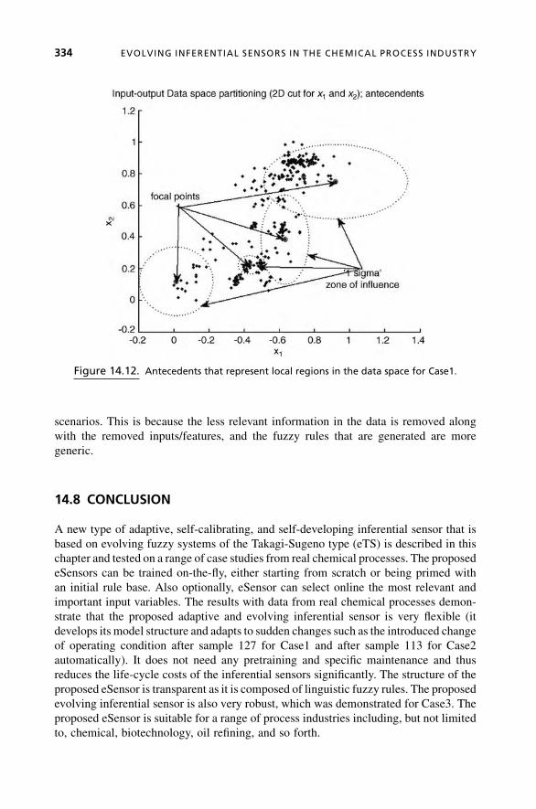
scenarios. This is because the less relevant information in the data is removed along

with the removed inputs/features, and the fuzzy rules that are generated are more

generic.

14.8 CONCLUSION

A new type of adaptive, self-calibrating, and self-developing inferential sensor that is

based on evolving fuzzy systems of the Takagi-Sugeno type (eTS) is described in this

chapter and tested on a range of case studies from real chemical processes. The proposed

eSensors can be trained on-the-fly, either starting from scratch or being primed with

an initial rule base. Also optionally, eSensor can select online the most relevant and

important input variables. The results with data from real chemical processes demon-

strate that the proposed adaptive and evolving inferential sensor is very flexible (it

develops its model structure and adapts to sudden changes such as the introduced change

of operating condition after sample 127 for Case1 and after sample 113 for Case2

automatically). It does not need any pretraining and specific maintenance and thus

reduces the life-cycle costs of the inferential sensors significantly. The structure of the

proposed eSensor is transparent as it is composed of linguistic fuzzy rules. The proposed

evolving inferential sensor is also very robust, which was demonstrated for Case3. The

proposed eSensor is suitable for a range of process industries including, but not limited

to, chemical, biotechnology, oil refining, and so forth.

Figure 14.12. Antecedents that represent local regions in the data space for Case1.


14.9 ACKNOWLEDGMENT

The authors would like to thank Mr. Xiaowei Zhou for performing the numerical

experiments.

14.10 REFERENCES

Angelov P. (2002). Evolving Rule Based Models: A Tool for Design of Flexible Adaptive Systems.

Heidelberg, New York: Springer-Verlag, ISBN 3-7908-1457-1.

Angelov P., D. Filev (2004). “An Approach to On-line Identification of Takagi-Sugeno Fuzzy

Models,” IEEE Trans. on System, Man, and Cybernetics, Part B—Cybernetics, Vol. 34, No. 1,

pp. 484–498, ISSN 1094-6977.

Angelov, P. (2006). “Machine Learning (Collaborative Systems),” patent (WO2008053161,

priority date—November 1, 2006).


2006 Int. Symposium on Evolving Fuzzy Systems, Ambleside, UK, September 7–9, 2006, IEEE

Press, pp. 29–35, ISBN 0-7803-9719-3.

Angelov, P., X. Zhou (2008). “On-Line Learning Fuzzy Rule-based System Structure from Data



Chen L., O. Bernard, G. Bastin, P. Angelov (2000). “Hybrid Modelling of Biotechnolo-gical

Process Using Neural Networks,” Control Eng. Practice, Vol. 8, No. 7, pp. 821–827.

Eriksson, L., E. Johansson, N. Wold, S. Wold (2001). Multi- and Megavariate Data Analysis:

Principles and Applications. Umea, Sweden: Umetrics Academy.

Fortuna L., S. Graziani, A. Rizzo, M. G. Xibilia (2007). “Soft Sensor for Monitoring and Control

of Industrial Processes.” InAdvances in Industrial Control Series (M. J.Grimble,M.A. Johnson

eds.). Springer Verlag: Berlin, Germany.

FukunagaK. (1990). Introduction to Statistical Pattern Recognition, 2nd edition, Academic Press,

San Diego, CA, USA, ISBN 0-12-269851-7.

Hastie T., R. Tibshirani, & J. Friedman (2001). TheElements of Statistical Learning: DataMining,

Inference and Prediction. Heidelberg, Germany: Springer-Verlag.

Hopner F., F. Klawonn (2000). “Obtaining Interpretable FuzzyModels from Fuzzy Clustering and

Fuzzy Regression.” Proc. 4th Int. Conf. on Knowledge Based Intelligent Engineering Systems

and Allied Technologies (KES), Brighton, UK, pp. 162–165.

Hornik K. (1990). “Approximation Capabilities of Multilayer Feedforward Neural Networks,”

Neural Networks, Vol. 4, pp. 251–257.

Kalman R. (1960). “A New Approach to Linear Filtering and Prediction Problems,” Transactions

of the ASME—Journal of Basic Engineering, Vol. 83, pp. 95–107.

Klinkenberg R., T. Joachims (2000). “Detection Concept Drift with Support Vector Machines.”

Proc. 7th Int. Conf. on Machine Learning (ICML), Morgan Kaufman, pp. 487–494.

Kordon A., G. Smits (2001). “Soft Sensor Development Using Genetic Programming.” Proc.

GECCO’2001, San Francisco, pp. 1346–1351.

Kordon A., G. Smits, A. Kalos, E. Jordaan (2003). “Robust Soft Sensor Development Using

Genetic Programming.” In Nature-Inspired Methods in Chemometrics (R. Leardi ed.).

Amsterdam, Holland: Elsevier, pp. 69–108.

REFERENCES 335

Koza J. (1992). Genetic Programming: On the Programming of Computers by Means of Natural

Selection. Cambridge, MA: MIT Press.

Li W., H. H. Yue, S. Valle-Cervantes, S. J. Qin (2000). “Recursive PCA for Adaptive Process

Monitoring,” Journal of Process Control, Vol. 10, No. 5, pp. 471–486.

Macias, J., Feliu, J., Bosch, A. (2003). “SimulationWorkbench between HYSYS Rigorous Model

and Its NN Extension: Case Study of a Complex Simulation with Re-circulation.” Proc. 4th

European Congress on Chemical Engineering, ECCE 4, ISBN: 84-88233-31-0.

Qin, S. J., H. Yue, R. Dunia (1997). “Self-Validating Inferential Sensors with Application to Air


Rallo R., J. Ferre-Gine, A. Arena, F. Girault (2004). “Neural Virtual Sensor for the Inferential

Prediction of Product Quality from Process Variables,”Computers and Chemical Engineering,

Vol. 26, pp. 1735–1754.

Saltelli, A., K. Chan, E. Scott (2001). Sensitivity Analysis, John Wiley and Sons Ltd., Chichester,

West Sussex, UK, ISBN 0-471-99892-3.

Smits G., M. Kotachenek (2004). “Pareto-Front Exploitation Symbolic Regression,” In Genetic

Programming Theory and Practice II (U. M. O’Reiley, T. Yu, R. Riolo, B. Worzel, eds).

New York: Springer, pp. 283–300.


IndustrialData SetsUsing ParetoGenetic Programming.” InGenetic Programming Theory and

Practice III (T., Yu, R. Riolo, B. Worzel,eds). New York: Springer, pp. 79–92.

Takagi T., M. Sugeno (1985). “Fuzzy Identification of Systems and Its Applications to Modeling

and Control,” IEEE Trans. on Systems, Man and Cybernetics, Vol. 15, No. 1, pp. 116–132.

Victor J., A. Dourado (2004). On-line Interpretability by Fuzzy Rule Base Simplification and

Reduction,” European Symposium on Intelligent Technologies, Hybrid Systems and Their

Implementation on Smart Adaptive Systems, EUNITE2004, Aachen, Germany.

Widmer G., M. Kubat (1996). “Learning in the Presence of Concept Drift and Hidden Contexts,”

Machine Learning, Vol. 23, No. 1, pp. 69–101.

YanW., H. Shao, X.Wang (2004). “Soft SensingModelling Based on Support VectorMachine and

Bayesian Model Selection,” Computers and Chemical Engineering, Vol. 28, pp. 1489–1498.

Zitzler E., L. Thiele (1999). “Multiobjective Evolutionary Algorithms: AComparative Case Study

and the Strength Pareto Approach,” IEEE Trans. on Evolutionary Computation, Vol. 3, No. 4,

pp. 257–271.


15

RECOGNITION OF HUMANGRASP BY FUZZY MODELING

R. Palm, B. Kadmiry, B. Iliev

15.1 INTRODUCTION

Over the past decade, the field of humanlike robotic hands has attracted significant

research efforts aiming at applications such as service robots and prosthetic hands, as

well as industrial applications. However, such applications are relatively few so far due to

the lack of appropriate sensor systems and some unsolved problems with human–robot

interaction. One reason is the difficult programming procedure due to the high

dimensionality of grasping and manipulation tasks. An approach to solve this problem

is programming by demonstration (PbD), which is used in complex robotic applications

such as grasping and dexterous manipulation.

In PbD, the operator performs a task while the robot captures the data by a motion-

capture device or a video camera and analyzes the demonstrated actions. Then the robot

has to recognize these actions and replicate them in the framework of a complex

application. One of the most complicated tasks is the recognition procedure because of

the ambiguous nature of human grasp. One of the techniques to copewith the recognition

problem is to use evolving fuzzy systems (EFSs) that are able to learn parameters online in

a self-developing and self-adapting manner. Important research has been done in the

fields of identification of TS-fuzzy models [1] and the adaptation of fuzzy rule bases

using online clusteringmethods [2]. A robotic application formobile robots in a dynamic

environment can be found in [3]. Different techniques for grasp recognition have been


and Nikola Kasabov


applied in PbD. Kang et al. [4] describe a system that observes, recognizes, and maps

human grasp to a robot manipulator using a stereo vision system and a data glove.

Zoellner et al. [5] use a data glovewith integrated tactile sensors where the recognition is

based on support vector machines (SVMs). Ikeuchi et al. [6] apply hidden Markov

models (HMMs) to segment and recognize grasp sequences. Ekvall and Kragic [7] also

use HMM methods and address the PbD problem using arm trajectory as an additional

feature for grasp classification. Li et al. [8] use singular value decomposition (SVD) for

the generation of feature vectors of human grasp and SVMs, which are applied to the

classification problem. Aleotti and Caselli [9] describe a virtual-reality-based PbD

system for grasp recognition where only final grasp postures aremodeled based on finger

joint angles. Palm and Iliev presented twomethods based on fuzzy models [10] and [11].

These twomethods can be seen as evolving fuzzy systems as they are able to learn robotic

behaviors or task primitives from experience. However, looking at the rich variety of

cited methods, it is evident that they do not provide equally successful results.

Therefore, three methods are compared with one another, two of them being already

described in detail in [10] and [11] and the third one being a hybrid method of fuzzy

clustering andHMMmethods.All threemethods startwith fuzzy time clustering. Thefirst

method, which is the simplest one, classifies a given test grasp using the distances of the

time clusters between the test grasp and a set of model grasps [10]. The second method,

which is more complex, is based on qualitative fuzzy recognition rules and solves the

segmentation problem and the recognition problem at once [11]. The third method deals

with fuzzy time clustering and grasp recognition usingHMMs [12]. All threemethods are

tested on the same set of grasp data in order to provide a fair comparison of the methods.

This chapter is organized as follows: Section 15.2 describes the experimental

platform consisting of a data glove and a hand simulation tool. Section 15.3 discusses

the learning of grasps by time-clustering and the training of model grasps. Section 15.4

describes the three recognition methods. Section 15.5 presents the experimental results

and gives a comparison of the three methods. Finally, section 15.6 draws some

conclusions and directions for future work.

15.2 AN EXPERIMENTAL PLATFORM FOR PBD

Robotic grasping involves two main tasks: segmentation of human demonstrations and

grasp recognition. The first task is to partition the data record into a sequence of episodes,

where each one contains a single grasp. The second task is to recognize the grasp

performed in each episode. Then the demonstrated task is (automatically) converted into

a program code that can be executed on a particular robotic platform (see Figure 15.1).

If the system is able to recognize the corresponding human grasps in a demonstration, the

robot will also be able to perform the demonstrated task by activating respective grasp

primitives (see Figure 15.2). The experimental platform consists of a hand-motion-

capturing device and a hand simulation environment. Themotions of the human operator

are recorded by a data glove (CyberGlove), which measures 18 joint angles in the hand

and the wrist (see [13]). Since humans mostly use a limited number of grasp types, the

recognition process can be restricted to certain grasp taxonomies, such as those

338 RECOGNITION OF HUMAN GRASP BY FUZZY MODELING

developed by Cutkosky [14] and Iberall [15]. Here, we use Iberall’s human grasp

taxonomy (see Figure 15.3).

To test the grasp primitives,we developed a simulationmodel of a five-fingered hand

with three links and three joints in each finger. The simulation environment allows us to

perform a kinematic simulation of the artificial hand and its interaction with modeled

objects.

Moreover, we can simulate recorded demonstrations of human operators and

compare them with the result from the execution of corresponding grasp primitives.

We tested the grasping of 15 different objects (see Figure 15.4), some of them belonging

to the same class in terms of an applied type of grasps. For example, cylinder and small

bottle correspond to cylindrical grasp, and sphere and cube to precision grasp, and so on.

Figure 15.1. Programming by demonstration of grasping tasks.

Figure 15.2. Learning of grasp primitives from human demonstrations.

AN EXPERIMENTAL PLATFORM FOR PBD 339

15.3 MODELING OF GRASP PRIMITIVES

15.3.1 Modeling by Time-Clustering

The recognition of a grasp type is achieved by a model that reflects the behavior of the

hand in time. In the following, an approach to learning human grasps from demonstra-

tions by time-clustering [10] is briefly described. The result is a set of grasp models for a

selected number of human grasp motions. According to section 15.2, a number of

experiments were performed in which time sequences for 15 different grasps were

collected using a data glove with 18 sensors (see [13]).

Each demonstration has been repeated several times to collect enough samples of

every particular grasp. The time period for a single grasp is about 3 seconds. From those

data, models for each individual grasp have been developed using fuzzy clustering and

Takagi-Sugeno fuzzy modeling [16].

The basic idea is described in the following [10]. We consider the time instants as

model inputs and the three finger joint angles as model outputs (for fingertip coordinates,

Figure 15.3. Grasp taxonomy by Th. Iberall [15].


see Figures 15.5 and 15.6). Let the angle trajectory of a finger be described by

qðtÞ ¼ fðtÞ ð15:1Þ

where q 2 R3; f 2 R3; t 2 Rþ . Linearization of (15.1) at selected time points ti yields

qðtÞ ¼ qðtiÞþDfðtÞDt

ti

� ðt�tiÞ ð15:2Þ

which is a linear equation in t:

qðtÞ ¼ Ai � tþ di ð15:3Þwhere

Ai ¼ DfðtÞDt

ti

2 R3 and di ¼ qðtiÞ�DfðtÞDt

ti

� ti 2 R3

Using (15.3) as a local linear model one can express (15.1) in terms of a Takagi-Sugeno

fuzzy model [17]:

qðtÞ ¼Xci¼1

wiðtÞðAi � tþ diÞ ð15:4Þ

Figure 15.4. Grasp primitives.

Figure 15.5. Block scheme of grasp modeling.

MODELING OF GRASP PRIMITIVES 341

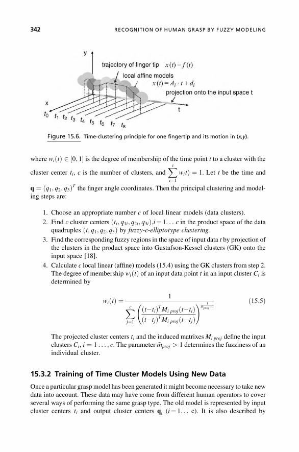
where wiðtÞ 2 ½0; 1� is the degree of membership of the time point t to a cluster with the

cluster center ti, c is the number of clusters, andXci¼1

witÞ ¼ 1. Let t be the time and

q ¼ ðq1; q2; q3ÞT the finger angle coordinates. Then the principal clustering and model-

ing steps are:

1. Choose an appropriate number c of local linear models (data clusters).

2. Find c cluster centers ðti; q1i; q2i; q3iÞ;i¼ 1. . . c in the product space of the data

quadruples ðt; q1; q2; q3Þ by fuzzy-c-elliptotype clustering.

3. Find the corresponding fuzzy regions in the space of input data t by projection of

the clusters in the product space into Gustafson-Kessel clusters (GK) onto the

input space [18].

4. Calculate c local linear (affine) models (15.4) using the GK clusters from step 2.

The degree of membership wiðtÞ of an input data point t in an input cluster Ci is

determined by

wiðtÞ ¼ 1

Xcj¼1

ðt�tiÞTMi projðt�tiÞðt�tjÞTMi projðt�tjÞ

! 1~mproj�1

ð15:5Þ

The projected cluster centers ti and the induced matrixesMi proj define the input

clusters Ci, i ¼ 1 . . . ; c. The parameter ~mproj > 1 determines the fuzziness of an

individual cluster.

15.3.2 Training of Time Cluster Models Using New Data

Once a particular grasp model has been generated it might become necessary to take new

data into account. These data may have come from different human operators to cover

several ways of performing the same grasp type. The old model is represented by input

cluster centers ti and output cluster centers qi (i¼ 1. . . c). It is also described by

Figure 15.6. Time-clustering principle for one fingertip and its motion in (x,y).


parameters Ai and bi of the local linear models. The old model was built by a time

sequence ½t1; t2; . . . ; tN � and a respective angle sequence ½q1; q2; . . . ; qN �. A new model

using new data ½~t1;~t2; . . . ;~tM � and ½~q1; ~q2; . . . ; ~qM � can be built by combining the

sequences ½t1; t2; . . . ; tN ;~t1;~t2; . . . ;~tM� and ½q1; q2; . . . ; qN ; ~q1; ~q2; . . . ; ~qM �. The result

is a model that involves properties of the old model and the new data. If the old sequence

of data is not available, a corresponding sequence can be generated by running the old

model with the time instants ½t1; t2; . . . ; tN � as inputs and the joint angles ½q1; q2; . . . ; qN �as outputs.

15.3.3 Modeling of Inverse Kinematics

In a similar way, the inverse kinematics of each finger for a particular grasp is modeled.

Let

xðtÞ ¼ fðqÞ; qðtÞ ¼ f�1ðxÞ ð15:6Þ

be the nonlinear direct and inverse transformation for a single finger where the inverse

transformation is not necessarily unique for the existing finger kinematics. From (15.6)

one can easily obtain the differential transformations

_xðtÞ ¼ JðqÞ _q; _qðtÞ ¼ Jþ ðxÞ _x ð15:7Þ

where JðqÞ ¼ qqqx is the Jacobian and J

þ ðxÞ is the pseudo-inverse Jacobian. Since xðtÞ or_xðtÞ, respectively, are already known from (15.4), the inverse kinematics in (15.7)

remains to be computed.

In order to avoid the time-consuming calculation of the inverse Jacobian at every

time instant, the inverse differential kinematics is approximated by a TS model

_qðtÞ ¼Xci¼1

wiðqÞJþi ðxiÞ _x ð15:8Þ

where wiðqÞ 2 ½0; 1� is the degree of membership of the angle vector q to a cluster with

the cluster centerqi, and Jþi ðxiÞ are the pseudo-inverse Jacobians in the cluster centers xi.

Due to the errorsDx ¼ xðtÞ�xmðtÞbetween the desired position xðtÞ and the real positionxmðtÞ, a correction of the angles is done using the analytical forward kinematics

xm ¼ fðqðtÞÞ of the finger (see Figure 15.7). This changes (15.8) into

_qðtÞ ¼Xci¼1

wiðxÞJþi ðxiÞð _xþK � ðxðtÞ�xmðtÞÞÞ ð15:9Þ

whereK is a scalar that has to be determined so that the optimization loop is stable. It has

to be emphasized that the correction or optimization loop using the forward kinematics

fðqðtÞÞ is started at every new time instant and stopswhen either a lower bound jjDxjj < eis reached or a given number of optimization steps is executed. The general control

scheme is shown in Figure 15.8. Kawato [19] used a related technique that suggests that

MODELING OF GRASP PRIMITIVES 343

humans use both kinematical and dynamical internal models in movement planning and

control. In our implementation, a grasp command activates the respective forward

dynamic model of type (15.6) to generate the desired trajectory in Cartesian space. The

desired joint space trajectories are obtained using the inverse kinematical model (15.8).

The grasping motion continues until contact with the object is established.

15.4 RECOGNITION OF GRASPS—THREE METHODS

In the previous section we showed that TS fuzzy models can be successfully used for

modeling and imitation of human grasp behaviors. Now, wewill show that they can also

be used for classification of grasps from recorded human demonstrations. If we just

observe captured motions of a human arm while executing several grasp actions it is

difficult to identify the exact moment when a grasp sequence starts and ends. Related

research shows that this task can be solved efficiently only by fusion of additional

information sources such as tactile sensing and vision (see [6] and [7]).

In the following, we present three different recognition methods, all of them based

on the time clustering of human grasps. The first method classifies a test grasp by

comparing the time clusters of the test grasp and a set of model grasps. The second

Figure 15.7. Inverse kinematics with correction.

Figure 15.8. Control architecture.


method uses fuzzy recognition rules for segmentation and recognition. The third method

classifies a test grasp using HMMs, which are applied to the output cluster centers of the

grasp models. It should be stressed that methods 1 and 2 are related; both of them use

distances between fuzzy clusters for recognition. Method 3 is a completely different

approach using a probability method for recognition and classification.

15.4.1 Recognition of Grasps Using the Distance between FuzzyClusters

Let the model of each grasp have the same number of clusters i ¼ 1 . . . c so that each

duration Tlðl ¼ 1 . . . LÞ of the lth grasp is divided into ðc�1Þ time intervals

Dti ¼ ti�ti�1, i¼ 2. . . c, of the same length. Let the grasps be executed in an environment

comparable to the modeled grasp in order to avoid calibration and rescaling procedures.

Furthermore let

Vmodel l ¼ ½Vindex;Vmiddle;Vring;Vpinkie;Vthumb�lVindex l ¼ ½q1; . . . ; qi; . . . ; qc�index l

..

.

Vthumb l ¼ ½q1; . . . ; qi; . . . ; qc�thumb l

qi ¼ ðq1i; q2i; q3iÞT

ð15:10Þ

wherematrixVmodel l includes the output cluster centersqi of everyfinger for the lth grasp

model. qi is the vector of joint angles of each finger. A model of the grasp to be classified

is built by the matrix

Vgrasp ¼ ½Vindex;Vmiddle;Vring;Vpinkie;Vthumb�grasp ð15:11Þ

A decision on the type of grasp is made by applying the Euclidean matrix norm

Nl ¼ kVm�Vgraspkl ð15:12Þ

The unknown grasp is classified to the grasp model with the smallest norm minðNlÞ,l ¼ 1 . . . L, and the recognition of the grasp is finished.

15.4.2 Recognition Based on Qualitative Fuzzy Recognition Rules

The identification of a grasp from a combination of grasps is based on a recognition

model. This model is represented by a set of recognition rules using the model grasps

mentioned in the previous section. The generation of the recognition model is based on

the following steps:

1. Computation of distance norms between a test grasp combination and the model

grasps involved

2. Computation of extrema along the sequence of distance norms

RECOGNITION OF GRASPS—THREE METHODS 345

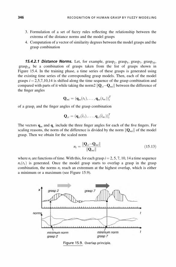
3. Formulation of a set of fuzzy rules reflecting the relationship between the

extrema of the distance norms and the model grasps

4. Computation of a vector of similarity degrees between the model grasps and the

grasp combination

15.4.2.1 Distance Norms. Let, for example, grasp2; grasp5; grasp7; grasp10;grasp14 be a combination of grasps taken from the list of grasps shown in

Figure 15.4. In the training phase, a time series of these grasps is generated using

the existing time series of the corresponding grasp models. Then, each of the model

grasps i¼ 2,5,7,10,14 is shifted along the time sequence of the grasp combination and

compared with parts of it while taking the norm2 kQci�Qmik between the difference ofthe finger angles

Qmi ¼ ðqmðt1Þ; . . . ; qmðtncÞÞTiof a graspi and the finger angles of the grasp combination

Qci ¼ ðqcið~t1Þ; . . . ; qcið~tncÞÞTiThe vectors qm and qc include the three finger angles for each of the five fingers. For

scaling reasons, the norm of the difference is divided by the norm kQmik of the model

grasp. Then we obtain for the scaled norm

ni ¼ kQci�QmikkQmik

ð15:13Þ

where ni are functions of time.With this, for each grasp i¼ 2, 5, 7, 10, 14 a time sequence

niðt1Þ is generated. Once the model grasp starts to overlap a grasp in the grasp

combination, the norms ni reach an extremum at the highest overlap, which is either

a minimum or a maximum (see Figure 15.9).

Figure 15.9. Overlap principle.


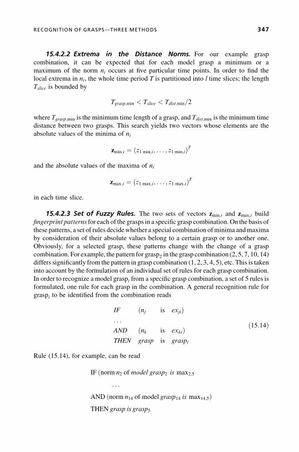
15.4.2.2 Extrema in the Distance Norms. For our example grasp

combination, it can be expected that for each model grasp a minimum or a

maximum of the norm ni occurs at five particular time points. In order to find the

local extrema in ni, the whole time period T is partitioned into l time slices; the length

Tslice is bounded by

Tgrasp;min < Tslice < Tdist;min=2

where Tgrasp;min is the minimum time length of a grasp, and Tdist;min is the minimum time

distance between two grasps. This search yields two vectors whose elements are the

absolute values of the minima of ni

zmin;i ¼ ðz1 min;i; . . . ; z1 min;iÞT

and the absolute values of the maxima of ni

zmax;i ¼ ðz1 max;i; . . . ; z1 max;iÞT

in each time slice.

15.4.2.3 Set of Fuzzy Rules. The two sets of vectors zmin;i and zmax;i build

fingerprint patterns for each of the grasps in a specific grasp combination.On the basis of

these patterns, a set of rules decidewhether a special combination ofminima andmaxima

by consideration of their absolute values belong to a certain grasp or to another one.

Obviously, for a selected grasp, these patterns change with the change of a grasp

combination. For example, the pattern for grasp2 in the grasp combination (2, 5, 7, 10, 14)

differs significantly from the pattern in grasp combination (1, 2, 3, 4, 5), etc. This is taken

into account by the formulation of an individual set of rules for each grasp combination.

In order to recognize a model graspi from a specific grasp combination, a set of 5 rules is

formulated, one rule for each grasp in the combination. A general recognition rule for

graspi to be identified from the combination reads

IF ðnj is exjiÞ. . .

AND ðnk is exkiÞTHEN grasp is graspi

ð15:14Þ

Rule (15.14), for example, can be read

IF ðnorm n2 of model grasp2 is max2;5

. . .

AND ðnorm n14 of model grasp14 is max14;5ÞTHEN grasp is grasp5


The full rule to identify grasp5 reads

IF ðn2 is max2;5ÞAND ðn5 is min5;5ÞAND ðn7 is max7;5ÞAND ðn10 is min10;5ÞAND ðn14 is min14;5ÞTHEN grasp is grasp5

ð15:15Þ

j¼ 2 . . . 14 are the indexes of the grasps in the grasp combination; i is the index of graspito be identified; exij indicate fuzzy sets of local extrema, which can be either minima

minij or maxima maxij . Extrema appear at the time points ~t ¼ tj at which model graspimeets graspj in the grasp combination with a maximum overlap.

Let the total extremum zex; tot be either a total minimum zmin; tot or a maximum

zmax; tot over all 5 rules and all time slices (see Figure 15.10):

zmin; tot ¼ minðzjmin;iÞ; zmax; tot ¼ maxðzjmax;i

Þj ¼ 1 . . . l; i ¼ 2; 5; 7; 10; 14

ð15:16Þ

Then a local extremum zjex;i can be expressed by the total extremum zex; tot and a weight

wji 2 ½0; 1�:

zjex;i ¼ wji � zex; tot; zjmin;i¼ wji � zmin; tot

zjmax;i¼ wji � zmax; tot; j; i ¼ 2; 5; 7; 10; 14

ð15:17Þ

Figure 15.10. Norms of a grasp sequences.


15.4.2.4 SimilarityDegrees. From the time plots in Figure 15.10 of the norms nifor the training sets, the analytical form of (15.15) for the identification of graspi is

chosen as follows:

ai ¼Yjmji;

mji ¼ Expð�jwji � zex; tot�zex ijÞzex i ¼ ðz1ex;i; . . . ; z1ex;iÞT

j ¼ 2; 5; 7; 10; 14 ð15:18Þ

ai ¼ ða1i; . . . ; aliÞT , ami 2 ½0; 1�;m ¼ 1; . . . ; l is a vector of similarity degrees between

themodel graspi and the individual grasps 2, 5, 7, 10, 14 in the grasp combination at the

time point tm. The vector zex;i represents the vector of either minima zmin;i or maxima

zmax;i of the norms ni, respectively.

The product operation in (15.18) represents theAND-operation in rules (15.15). The

exponential function in (15.18) is a membership function indicating the distance of a

norm ni to a local extremum wji � zex; tot. With this, the exponential function reaches its

maximum at exactly that time point tm when graspi in the grasp combination has its local

extremum (see, e.g., Figure 15.11). Sincewe assume the time points for the occurrence of

the particular grasps in the combination to be known, we also know the similarity degrees

am;i between the model graspi and grasps 2, 5, 7, 10, 14 at these time points. If, for

Figure 15.11. Grasp membership functions.


example, grasp5 occurs at time point tm in the grasp combination, then we obtain for

am;5 ¼ 1.

All the other grasps lead to smaller values of ak;i ¼ 1; k ¼ 2; 7; 10; 14.With this, the

type of grasp is identified and the grasp recognition is finished.

15.4.3 Recognition Based on Time-Cluster Models and HMM

The task is to classify an observation sequence of a test grasp given a set of observation

sequences of model grasps using HMMs. The HMMs used here are of discrete nature,

which requires the formulation of a number discrete states and discrete observations. One

condition for the use of HMMs in our approach is that all model grasps and the test grasp

to be recognized are modeled by the time-clustering described earlier.

The elements of a discrete HMM can be described in the compact notation [20]:

l ¼ ðA;B; p;N;MÞ ð15:19Þ

where N is the number of states S, M is the number of observations O, A ¼ faijg is thematrix of state transition probabilities,B ¼ fbijg is the observation symbol probability of

symbolOk in state j, and p is the initial state distribution vector. To prepare the HMM for

the recognition, a number of steps have to be done:

Step 1:Determine a number N of states S. The states need not be directly connected

with a physical meaning, but it is of great advantage to do so.

Therefore, M¼ 5 states are chosen, getting the following labels:

State S1: open hand

State S2: half-open hand

State S3: middle position

State S4: half-closed hand

State S5: closed hand

Step 2: Generate a number M of discrete observations O. To generate discrete

observations, one first has to deal with the continuous observations, meaning

the output cluster centers in Vgrasp and the corresponding joint angles qi. It should

be mentioned that the clustering process leads to vectors of cluster centers whose

elements, although being “labelled” by a time stamp, are not sorted in increasing

order of time. Since clustering of several grasps is done independently of each

other, the orders of time stamps of the cluster centers are in general different. This

makes a comparison of test clusters Vgrasp and model clusters Vmodel impossible.

Therefore, after time clustering has been performed, the output clusters have to be

sorted in increasing order of time. In the following, cluster centers are assumed to

be sorted in that way. Next, one has to transform the continuous output cluster

centers Vmodel (i), i¼ 1. . .10 of the model into discrete numbers or labels. If one

attached to each cluster center an individual label, one would obtain

M ¼ 10 15 ¼ 150 observation labels (10-number of clusters, 15-number of

grasps). This number of observations is unnecessarily high because some of the


cluster centers form almost identical hand poses. Therefore, two observations are

reserved for the starting pose and ending pose of all grasps since it can be assumed

that every grasp starts and ends with nearly the same pose. Three poses for each

grasp are then chosen at cluster numbers (3,5,6), which makes

M ¼ 3 15þ 2 ¼ 47 observations. The result is obviously a set of possible

observations labeled by the numbers 1 . . . 47, representing 47 poses of 15 time-

clustering models of grasps. In order to label a specific pose of a given grasp, one

finds the minimal norms

IjðiÞ ¼ minðkVgraspj ðiÞ�out1k; . . . ; kVgraspj ðiÞ�out47kÞ; i ¼ 1 . . . 10 ð15:20Þ

where IjðiÞ 2 ½1 . . . 47� is the observation label, i 2 ½1 . . . 10� is the number of a

time cluster for test grasp j 2 ½1 . . . 15�, OðkÞ ¼ Vmodel mðlÞ, k 2 ½1 . . . 47� is thekth observation, m 2 ½1 . . . 15� is a corresponding model grasp, and

l 2 ½2; 3; 5; 6; 9� is a corresponding number of a time cluster in model grasp

m. This procedure is done for all model grasps Vmodel with the result of 15

sequences IjðiÞ of 10 observations each, and for the test grasp Vgrasp to be

recognized.

Step 3: Determine the initial matrixes A 2 RMM , B 2 RNM and the initial state

distribution vector p 2 R1N. Since in the experiments the hand always starts to

move from almost the same pose and keeps on moving through the states defined

above, we can estimate both the initial matrixes A and B, and the initial state

distribution vector p easily.

Step 4: Generate 15 observation sequences Otrain 2 R1015 for the 15 model grasps

according to step 2.

Step 5:Generate 1 observation sequenceOtest 2 R101 for the test grasp according tostep 2.

Step 6: Train the HMM with every model sequence Otrain separately, using the

iterative expectation-modification (EM), procedure, also known as the Baum-

Welch method. The training process evaluates a log-likelihood LL of the trained

model during iteration and stops as the change of LL undergoes a certain

threshold. Observe here that LL � 0.

Step 7: Classify the observation sequence Otest by evaluating the log-likelihood

LL of the mth trained HMM for a model grasp m given the test data Otest. In

addition, the most probable sequence of states using the Viterbi algorithm is

computed.

Step 8: Compute the most probable model grasp number m to be closest to the test

model by computing maxðLLiÞ, i¼ 1. . .15. With step 8, the grasp recognition is

completed.

15.5 EXPERIMENTS AND SIMULATIONS

In this section, we present the experimental evaluation of the proposed approach for

modeling and classification of grasps. We tested 15 different grasps:

EXPERIMENTS AND SIMULATIONS 351

1. Cylinder

2. Big bottle

3. Small bottle

4. Hammer

5. Screwdriver

6. Small ball

7. Big ball

8. Precision grasp (sphere)

9. Precision grasp (cube)

10. Plane (1 CD-ROM)

11. Plane (3 CD-ROMs)

12. Fingertip grasp (small ball)

13. Fingertip grasp (big ball)

14. Fingertip grasp (can)

15. Penholder grasp

and recorded five instances for each one to perform themodeling.Here, three of the tested

grasps and their simulations are shown. The motion trajectories are generated according

to the scheme in Figure 15.8.

The grasp is completed when the fingers establish contact with the object as in the

demonstrations:

. Grasp a CD-ROM (plane; see Figures 15.12, 15.13)

. Grasp a small bottle (cylinder; see Figures 15.14, 15.15)

. Grasp a big ball (sphere; see Figures 15.16, 15.17)

15.5.1 Modeling of the Fingertip Trajectories

For each grasp and finger, 10 fingertip position models with 10 cluster centers have been

generated from the collected data. Furthermore, 3 inverse Jacobianmodels for each grasp

Figure 15.12. CD-ROM grasp.


Figure 15.14. Small bottle grasp.

Figure 15.13. CD-ROM grasp simulation.

Figure 15.15. Small bottle grasp simulation.


behavior and finger with 3 cluster centers have been built. Since there are 33 time steps

for the whole motion, time clustering results in the cluster centers

t1 ¼ 2:04; 5:43; 8:87; 12:30; 15:75; 19:19; 22:65; 26:09; 29:53; 32:94

These are complemented by the corresponding cluster centers for the x,y,z coordinates of

the fingertips. This equidistant spacing can be found for every individual grasp primitive

as a result of the time clustering. Figures 15.18 and 15.19 present the example of the index

finger performing the task “grasp CD-ROM.” Figures 15.20–15.23 show the modeling

results for the middle, ring, and pinkie finger, and the thumb. All results show a good or

even excellent modeling quality.

15.5.2 Grasp Segmentation and Recognition

In this subsection, we present the experimental evaluation of the three proposed

approaches for recognition of human grasp behaviors.

Figure 15.16. Big ball grasp.

Figure 15.17. Big ball grasp simulation.


15.5.2.1 Method 1: Distance between Fuzzy Clusters. The experimental

results are divided into three groups of recognition rates:

1. Grasps with a recognition rate � 75%

2. Grasps with a recognition rate < 75% . . . � 50%

3. Grasps with a recognition rate < 50%

Table 15.1 shows the recognition rates for method 1. The first group with a recognition

rate � 75% is the largest one, where 4 of 7 grasps show a recognition rate 100%. The

equally large groups 2 and 3 follow. The experimental results confirm the assumption that

distinct grasps can be discriminated quite well from each other, whereas the discrim-

ination between similar grasps is difficult. Therefore, merging of similar grasps and

Figure 15.19. Index finger time plots.

Figure 15.18. Trajectories of index finger.


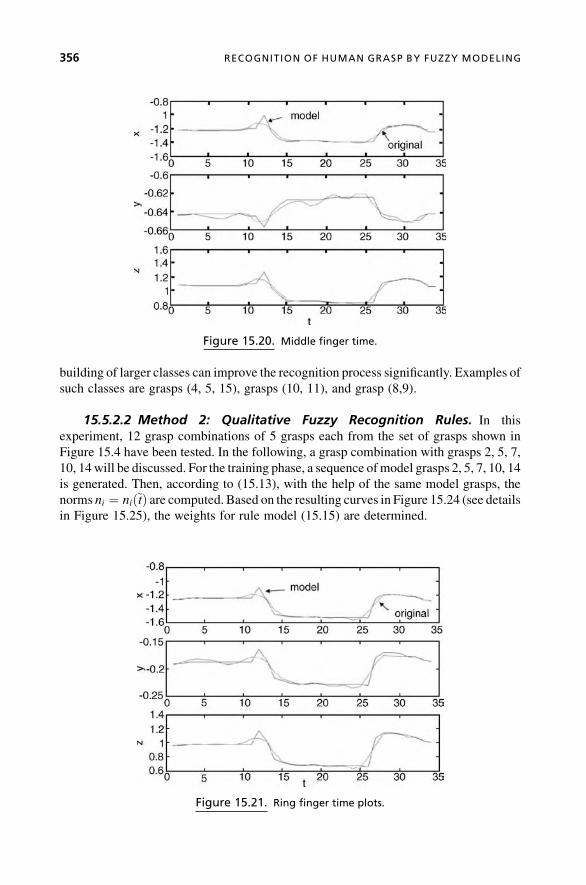
building of larger classes can improve the recognition process significantly. Examples of

such classes are grasps (4, 5, 15), grasps (10, 11), and grasp (8,9).

15.5.2.2 Method 2: Qualitative Fuzzy Recognition Rules. In this

experiment, 12 grasp combinations of 5 grasps each from the set of grasps shown in

Figure 15.4 have been tested. In the following, a grasp combination with grasps 2, 5, 7,

10, 14will be discussed. For the training phase, a sequence ofmodel grasps 2, 5, 7, 10, 14

is generated. Then, according to (15.13), with the help of the same model grasps, the

norms ni ¼ nið~tÞ are computed. Based on the resulting curves in Figure 15.24 (see details

in Figure 15.25), the weights for rule model (15.15) are determined.

Figure 15.21. Ring finger time plots.

Figure 15.20. Middle finger time.


The training results in the table in Figure 15.26 show that both the starting points and

the types of grasps 5, 7, 10, and 14 can be reliably recognized. Grasp 2, however, shows

rather high numbers at other time points, too,meaning that the recognition of this grasp is

less reliable. A test sample of the same grasp combination confirms this assumption:

There are good results for grasps 5, 7, 10, and 14 but a different (wrong) result for grasp 2

(see Figure 15.27). Many tests with other grasp combinations have shown that some

grasps can be more reliably recognized than others. Grasps with distinct maxima and

minima in their ni patterns can be recognized better than thosegraspswithout this feature.

In addition to the above example, another combination with a high recognition rate is

grasp(1,13,12,8,10), where grasps 1, 12, 8, and 10 are reliably recognized. In the

Figure 15.23. Thumb time plots.

Figure 15.22. Pinkie finger time plots.


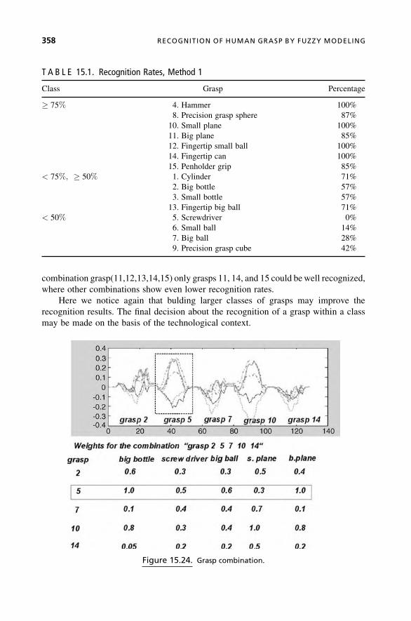
combination grasp(11,12,13,14,15) only grasps 11, 14, and 15 could bewell recognized,

where other combinations show even lower recognition rates.

Here we notice again that bulding larger classes of grasps may improve the

recognition results. The final decision about the recognition of a grasp within a class

may be made on the basis of the technological context.

T A B L E 15.1. Recognition Rates, Method 1

Class Grasp Percentage

� 75% 4. Hammer 100%

8. Precision grasp sphere 87%

10. Small plane 100%

11. Big plane 85%

12. Fingertip small ball 100%

14. Fingertip can 100%

15. Penholder grip 85%

< 75%; � 50% 1. Cylinder 71%

2. Big bottle 57%

3. Small bottle 57%

13. Fingertip big ball 71%

< 50% 5. Screwdriver 0%

6. Small ball 14%

7. Big ball 28%

9. Precision grasp cube 42%

Figure 15.24. Grasp combination.


Table 15.2 shows the recognition rates for method 2. It could be shown that grasps

with distinct maxima andminima in their ni patterns can be recognized better than grasps

without this feature. Reliable grasps are also robust against variations in the time span of

an unknown test grasp compared to the time span of the respective model grasp. Our

results show that this method can handle a temporal difference up to 20%. The first group

Figure 15.26. Grasp combination, training results.

Figure 15.25. Details of grasp 5.


with recognition rate � 75% is again the largest one, where 3 of 8 grasps show

recognition rate 100%.

15.5.2.3 Method 3: Time Cluster Models and HMM. The detailed choice of

the number of states and observations has already been described in steps 1 and 2 of the

Figure 15.27. Grasp combination, test results.



� 75% 4. Hammer 100%

5. Screwdriver 93%



10. Small plane 100%

11. Big plane 88%



< 75; � 50% 1. Cylinder 55%

2. Big bottle 60%

3. Small bottle 66%

6. Small ball 55%

< 50% 7. Big ball 16%




description of the algorithm. The recognition rates for method 3 are shown in Table 15.3.

Here, the second group is the largest one, with recognition rate<75%,� 50%, followed

by the first group, where 2 of 5 grasps show recognition rate 100%, and then by the third

one.

15.5.2.4 Comparison of the Three Methods. For more than half of the grasp

primitives, all threemethodsprovidesimilar results.This is true forgrasps1,2,3,4,7,8,10,

and15.However, similarities betweengraspsmaygive space formisinterpretations,which

explains the low percentages for some grasps (e.g., grasps 5 and 9 in method 1 or grasps 5

and 8 in method 3). Looking at the first groups in Tables 15.1, 15.2, and 15.3, group 1,

method 1 is the most successful, and is also a solution with the easiest implementation.

Then follows method 2, with quite a high implementation effort, and finally method 3,

based onHMM. It should be stated that theHMMprinciplemay allow some improvement

of the results, especially in the case of an extended sensory in the experimental setup.

15.6 CONCLUSION

The goal of grasp recognition is to develop an easy way of programming by demon-

stration of grasps for a humanoid robotic arm. One promising way to cope with the

recognition problem is to use evolving fuzzy systems, which are self-developing and

self-adapting systems. In this chapter, three different methods of grasp recognition are

presented. Grasp primitives are captured by a data glove and modeled by TS-fuzzy

models. Fuzzy clustering and modeling of time-and-space data are applied to the

modeling of the finger joint angle trajectories (or fingertip trajectories) of grasp

primitives. The first method, being the simplest one, classifies a human grasp by



� 75% 4. Hammer 100%


10. Small plane 85%



< 75%; � 50% 1. Cylinder 71%

2. Big bottle 57%

3. Small bottle 71%

5. Screwdriver 71%

6. Small ball 57%

11. Big plane 57%



< 50% 7. Big ball 0%


CONCLUSION 361

computing the minimum distance between the time clusters of the test grasp and a set of

model grasps. In the secondmethod, a qualitative fuzzymodel is developed,with the help

of which both a segmentation and a grasp recognition can be achieved. These first two

methods can be seen as evolving fuzzy systems, whereas the third method uses hidden

Markovmodels for grasp recognition. A comparison of the three methods shows that the

first method is the most effective method, followed by the second and third approaches.

To improve the PbD process, these methods will be further developed for the

recognition and classification of operator movements in a robotic environment using

more sensory information about the robot workspace and the objects to be handled.

15.7 REFERENCES

1. P. Angelov, D. Filev, “An approach to On-line Identification of Takagi-Sugeno Fuzzy

Models,” IEEE Trans. on Syst., Man, and Cyb., part B, Vol. SMC-34, No. 1, pp.

484–498, January/February 2004.

2. P. Angelov, R. Buswell, “Identification of Evolving Rule-Based Models,” IEEE Trans. on

Fuzzy Systems, Vol. SMC-34. No. 1, pp. 667–677, October 2002.

3. N. Kubota, Y. Nojima, F. Kojima, “Local Episode-Based Learning of a Mobile Robot in a

Dynamic Environment,” IEEE Trans. on Fuzzy Systems, Dynamic Systems Approach for

Embodiment and Sociality—From Ecological Psychology to Robotics. Int. Series on Ad-

vanced Intelligence, pp. 318–322, 2003.

4. S. B. Kang, K. Ikeuchi, “Towards Automatic Robot Instruction from Perception: Mapping

Human Grasps to Manipulator Grasps,” IEEE Trans. on Robotics and Automation, Vol. 13,

No. 1, 1997.

5. R. Zoellner, O. Rogalla, R. Dillmann, J.M. Zoellner, “Dynamic Grasp Recognition within the

Framework of Programming by Demonstration.” Proc. Robot and Human Interactive

Communication, 10th IEEE International Workshop, Bordeaux, Paris, France, September

18–21, 2001, IEEE.

6. K. Ikeuchi, K. Bernardin, K. Ogawara, R. Dillman, “A Sensor Fusion Approach for

Recognizing Continuous Human Grasp Sequences Using Hidden Markov Models,” IEEE

Trans. on Robotics, Vol. 21, No. 1, February 2005.

7. S. Ekvall, D. Kragic, “Grasp Recognition for Programming by Demonstration.” Proc. Int.

Conf. Robotics and Automation, ICRA 2005, Barcelona, Spain, 2005.

8. Ch. Li, L.Khan, B. Prabhaharan, “Real-TimeClassification ofVariable LengthMulti-attribute

Motions,” Knowledge and Information Systems, DOI 10.1007/s10115-005-0223-8, 2005.

9. J. Aleotti, S. Caselli, “Grasp Recognition in Virtual Reality for Robot Pregrasp Planning by

Demonstration.” ICRA 2006—Int. Conf. on Robotics and Automation, Orlando, Florida, May

2006, IEEE.

10. R. Palm, B. Iliev, “Learning of Grasp Behaviors for an Artificial Hand by Time Clustering and

Takagi-Sugeno Modeling.” Proc. FUZZ-IEEE 2006—IEEE Int. Conf. on Fuzzy Systems,

Vancouver, BC, Canada, July 16–21, 2006, IEEE.

11. R. Palm, B. Iliev. “Segmentation and Recognition of Human Grasps for Programming-by-

Demonstration Using Time Clustering and Takagi-Sugeno Modeling.” Proc. FUZZ-IEEE

2007—IEEE Int. Conf. on Fuzzy Systems, London, UK, July 23–26, 2007, IEEE.


12. R. Palm, B. Iliev, “Grasp Recognition by Time-Clustering, Fuzzy Modeling, and Hidden

MarkovModels (HMM):AComparative Study.”Proc. FUZZ-IEEE2008—IEEE Int. Conf. on

Fuzzy Systems, Hong Kong, June 1–6, 2008, IEEE.

13. H. H. Asada, J. R. Fortier, “Task Recognition and Human–Machine Coordination through the

Use of an Instrument-Glove,” Progress Report No. 2–5, pp. 1–39, March 2000.

14. M. Cutkosky, “On Grasp Choice, Grasp Models, and the Design of Hands for Manufacturing

Tasks,” IEEE Trans. on Robotics and Automation, Vol. 5, No. 3, 1989.

15. Thea Iberall, “Human Prehension and Dexterous Robot Hands,” Int. J. Robotics Research,

Vol. 16, pp. 285–299, 1997.

16. R. Palm, Ch. Stutz, “Generation of Control Sequences for a Fuzzy Gain Scheduler,” Int. J.

Fuzzy Systems, Vol. 5, No. 1, pp. 1–10, March 2003.

17. T. Takagi, M. Sugeno, “Identification of Systems and Its Applications to Modeling and

Control.” IEEE Trans. on Syst., Man, and Cyb., Vol. SMC-15, No. 1, pp. 116–132, January/

February 1985.

18. D. E. Gustafson, W. C. Kessel, “Fuzzy Clustering with a Fuzzy Covariance Matrix.” Proc.

1979 IEEE CDC, pp. 761–766, 1979.

19. M. Kawato, “Internal Models for Control and Trajectory Planning,” Current Opinion in

Neurobiology, No. 9, pp. 718–727, 1999.

20. L. R. Rabiner, “A Tutorial on Hidden Markov Models and Selected Applications in Speech

Recognition.” Proc. IEEE, Vol. 77, No. 2, pp. 257–286, February 1989.

REFERENCES 363

16EVOLUTIONARY

ARCHITECTURE FORLIFELONG LEARNING ANDREAL-TIME OPERATION INAUTONOMOUS ROBOTS

R. J. Duro, F. Bellas, J. A. Becerra

16.1 CHAPTER OVERVIEW

This chapter deals with evolution in the creation of a cognitive architecture for robots to

be able to learn and adapt throughout their lifetime. The emphasis of the architecture is

placed on modularity, progressive construction, and real-time adaptation to changes in

the environment, in the robot itself or in its motivations. As in other explicit cognitive

architectures, there is a part dealing with models (of the world, of the robot itself, of its

satisfaction. . .) and another part dealing with the generation of actions. Models must

adapt to changing circumstances and they must be remembered and generalized in order

to be reused. Actions and sequences of actions, on the other hand, must be generated in

real time so that the robot can copewith the environment and survive. In this line, the basic

idea of the system involves modular and incremental neural network–based architectures

for robot controllers that are in charge of the actions and reactions of the robots, and a

cognitive mechanism, based on evolutionary techniques, that permits learning about the

world and the robot itself and using this information to provide a framework for selecting

and modifying the controllers through lifelong interaction with the world, leading to the

ability of the robots to adapt to changing environments, goals, and circumstances. With

this combination, an evolutionary architecture is proposed for autonomous robots to

create complex behavior controllers that provide quick real-time response and that can be


and Nikola Kasabov


adjusted or even developed during the robot’s lifetime. Several examples of the use of

these types of architectures and their elements are presented and discussed.

16.2 INTRODUCTION

When dealingwith the problem of robots that are supposed to be autonomous, and leaving

aside the whole discussion on body–mind interaction (for this topic, see the excellent

review in [1]), a question arises on how to obtain the complex adaptive control system that

is required. A control system such as the one that is necessary for autonomy is really

something that goes beyond traditional control in terms of the specifications or require-

ments. These additional requirements imply the ability to learn the control function from

scratch, the ability to change or adapt it to new circumstances, and the ability to interact

with the world in real time while performing the aforementioned processes and, in some

instances, even to change the objectives that guide the control system.

Consequently, and to differentiate it from traditional control systems, these struc-

tures are usually called cognitive systems or mechanisms and in this chapter we will be

dealing with ways to apply evolution as an intrinsic element within these structures.

Cognition, as defined in [2], is “The mental process of knowing, including aspects

such as awareness, perception, reasoning, and judgment.” According to [3], cognitive

systems can be taken as “a collection of emerging information technologies inspired by

the qualitative nature of biologically based information processing and information

extraction found in the nervous system, human reasoning, human decision-making, and

natural selection.” To this we think it is very pertinent to add that a cognitive system

makes no sense without its link to the real (or virtual) world in which it is immersed and

which provides the data to be manipulated into information, requiring, consequently, the

capability of acting and sensing.

It is from these broad definitions that the actual implementations of cognitive

systems must arise, and there are several elements that should be taken into account. On

one hand we have the mental process of knowing, that is, in more mathematical terms, of

extracting models from data. These models can be employed in the process of decision

making so that appropriate actions may be taken as a function of sensing andmotivation.

On the other, we have the decision-making process itself, and, in robotics, a decision is

always related to an action or sequence of actions. In a sense, the models must be used in

order to decide the appropriate actions so as to fulfill the agent’s motivations. It is in how

the model-making process and the action determination process takes place that

cognitive mechanisms differ from each other.

To select actions is to explore the action space trying to fulfill the motivations or

objectives, that is, to find the optimal action for the agent. To create models is to try to

minimize the difference between the reality that is being modeled and the predictions

provided by themodel. Consequently, it is clear that a cognitivemechanismmust involve

some type of optimization strategy or algorithm. One of the most promising avenues

in this line, especially as the search spaces are not really known beforehand and are

usually very complex, is to employ stochasticmultipoint search techniques, in particular,

artificial evolution.

366 EVOLUTIONARY ARCHITECTURE FOR LIFELONG LEARNING

In the field of autonomous robotics, evolutionary algorithms have been widely

applied to obtain controllers due to their adequateness for providing robust solutions

while minimizing the knowledge imposed by the designer. In fact, over the past two

decades, evolutionary robotics [4] has been one of the most active fields in the area of

autonomous robotics in terms of the number of publications on this topic.

However, most approaches presented take a static point of view regarding the

controllers or cognitive mechanisms obtained. That is, evolution is used as a tool to

obtain different types of data and information processing structures that are adapted to

a particular robot, environment, and tasks, and, once obtained, these structures hardly

change during the operation of the robot; they are mostly static [4]. In this chapter we

consider a different problem: how to obtain a cognitive mechanism that uses evolution

intrinsically to allow the robot cognitive system to adapt throughout its lifetime to

changing circumstances in terms of environment, objectives, and even of the robot itself.

Obviously, the ideal situationwith respect to designer workwould be for the robot to start

interacting with the world with no information and for it to be able to autonomously

construct its models and behaviors.

In the literature dealing with this problem, solutionsmay be found that use evolution

in a sort of lifelong learning process that starts from scratch, without any initial

knowledge provided to the robot. That is, the evolutionary algorithm is executed in

real time in the real robot, so that the improvement of the controller occurs in the genetic

algorithm’s time scale. Relevant examples of this approach are Watson et al. and their

embodied evolution system [5], where the authors use a population of physical robots that

autonomously reproduce while situated in their task environment; Nehmzow’s PEGA

algorithm [6], where the author presents experiments with a group of autonomous

mobile robots that learn to perform fundamental sensory-motor tasks through a collab-

orative learning process, or Floreano et al.’s coevolution system [7], where two Khepera

robots, one a predator and one the prey, interact with each other in a competitive way,

so that changes in the behavior of one agent drive further adaptation in the other.

However, few examples can be found following a pure lifelong-learning approach,

mainly because the evolutionary techniques applied in real robots that learn from

scratch require a very robust and complex learning system. The main problem is that

initial solutions are poor and the real robot could be damaged when using these initial

controllers to select an action. In addition, the learning system must be designed

minimizing the interference of the evolutionary process on the task; that is, the robot

must work in real time without pauses or speed limitations as a consequence of the time

taken up by evolution.

To minimize these problems, different authors have proposed, as an alternative to

lifelong learning, the application of an initial training stage where the robot works in

a controlled fashion and learns a limited number of tasks prior to real-time operation.

This way, when the robot starts with its task in the real world, it has a knowledge base in

terms of simple controllers that can be improved or adapted during its lifetime, if needed.

Within this approach, the solutions that can be found in the literature could be divided

into two main groups: authors that use the real robot for the training stage and authors

that use a simulator. In the first case, the real robot is used to estimate the fitness of the

individuals in the evolutionary algorithm for a particular task. Once the task is learned,

INTRODUCTION 367

the controller obtained is stored and a new learning process starts with the aim of learning

another. Obviously, this is a very designer-dependent approach where the teaching

process is highly time consuming. On the other hand, the solutions obtained are very

robust because they have been created in the same conditions the robot will find during its

real-time operation. Examples of this approach are Horny et al.’s [8] project to develop

efficient gaits in an AIBO robot or Marocco et al.’s [9] active vision system for mobile

robots.

Many more authors can be found that have used some kind of simulation stage to

obtain the controllers, mainly because this procedure permits complete control over the

environment, as well as carrying out a larger number of tests, avoiding in both cases all

the problems derived from the use of real robots. Within this approach wemust point out

the work of Wilson et al. [10], where the evolution in simulation and the real world are

interleaved. Initially, the authors produced primitive behaviors in simulation that were

tested on the physical robot. In later stages, these basic behaviors were randomly

concatenated to create sequences of behaviors. Another relevant approach is the

application of anytime learning [11] to hexapod robots, developed by Parker et al. [12],

where evolution took place in simulation and the best solution was sent to the physical

robot periodically. The information provided by the real robot application was used to

modify the genetic algorithm itself.

Finally, Walker [13] et al. have developed an approach to investigate the relative

contributions to robot performance of the training stage and lifelong learning. In this

case, the authors make use of a standard genetic algorithm for the training phase and

an evolutionary strategy for the real-time application stage. In their work, they conclude

that the real application stage improves the performance of a trained robot controller

in dynamic environments, and that the initial knowledge is very important for the

performance of the lifelong phase. In this line, in a recent review paper [14], Walker has

noted the observed advantages of using a combination of an initial training phase where

a knowledge base is created and a lifelong learning phase where the robot can adapt this

knowledge to the dynamics of real operation.

All of the aforementioned research, however, is based on consideration of the

autonomous robot as a system to be controlled and not really a cognitive system in terms

of having an internal structure that allows it to autonomously train and retrain itself—a

structure that allows the robot to have some type of modifiable internal representation of

its world, itself, and its objectives so that it can really apply cognitive strategies to solving

the problems it encounters throughout its lifetime as opposed to just following a set of

cleverly obtained recipes for particular situations in which it has been trained.

In this chapter, we provide an overview of what would be required as a first step

toward a cognitive robot and, in this line, one that can learn throughout its lifetime in an

adaptive manner. In particular, we will describe an approach that considers evolution an

intrinsic part of the cognitive system and that allows a robot to be able to learn different

tasks and objectives. Taking the process one step further, wewill incorporate the concept

of controller and controller architecture into cognition as a way to implement actions

and behaviors on the part of the robot; in particular, behaviors that are repeatedly and

successfully used will become reflex in terms of not having to go through the whole

cognitive process in order to activate them under particular circumstances. It is important


to note that a controller architecture that can be used within a cognitive system must

verify a series of requirements in order to be able to fully exploit its potential. The

architecture must be modular so that different behaviors may be combined to create new

ones, thus generating a structure that can grow depending on requirements without

having to relearn all from scratch, and parts of which may be reused as needed. In

addition there must be amechanism to gradually go from one behavior to another, so that

combinations of behaviors may be regulated.

The chapter is organized as follows: Section 16.3 describes the basic evolutionary

cognitive system and explains its general operation, including some comments on the

requirements for the evolutionary algorithms employed. Section 16.4 provides an

introduction to the behavior-based controller architecture that will act as a base for the

actuation part of the cognitive mechanism. Section 16.5 is devoted to the presentation

of some examples of the application of the cognitive architecture to real robots and a

discussion of its operation. Finally, Section 16.6 provides some conclusions and

comments on future work that is necessary in this line.

16.3 LIFELONG LEARNING EVOLUTIONARY ARCHITECTURE:THE MULTILEVEL DARWINIST BRAIN

Themultilevel Darwinist brain (MDB) is a general cognitive architecture first presented

in [15], that permits automatic acquisition of knowledge in a real agent through

interaction with its environment, so that it can autonomously adapt its behavior to

achieve its design objectives. To achieve this requirement, we have resorted to classical

biopsychological theories byChangeaux [16], Conrad [17], and Edelman [18] in the field

of cognitive science relating the brain and its operation through a Darwinist process.

All of these theories lead to the same concept of cognitive structure based on the brain

adapting its neural connections in real time through evolutionary or selectionist

processes.

The MDB can be formalized through a cognitive model, which is a particulari-

zation of the standard abstract architectures for agents [19]. In this case, a utilitarian

cognitive model was adopted that starts from the premise that, to carry out any task, a

motivation (defined as the need or desire that makes an agent act) must exist that guides

the behavior as a function of its degree of satisfaction. From this basic idea, the concepts

of action, world, and internal models (W and I), satisfaction model (S) and action–

perception pairs (sets of values made up by the sensorial inputs and the satisfaction

obtained after the execution of an action in the real world) are used to construct a

cognitive mechanism. Two processes must take place in a real non-preconditioned

cognitive mechanism: (1) modelsW, I, and Smust be obtained as the agent interacts with

theworld, and (2) the best possible actions must be selected through some sort of internal

optimization process using the models available at that time to determine fitness.

Thus, formalizing in general, the external perception e(t) of an agent is made up of

the sensory information it is capable of acquiring through its sensors from the envi-

ronment in which it operates. The environment can change due to the actions of the agent

or to factors uncontrolled by the agent. Consequently, the external perception can be

LIFELONG LEARNING EVOLUTIONARY ARCHITECTURE 369

expressed as a function of the last action performed by agent A(t� 1), the sensory

perception it had of the external world in the previous time instant e(t� 1), and a

description of the events occurring in the environment that are not due to its actions

Xe(t� 1) through a function W:

eðtÞ ¼ W ½eðt� 1Þ; Aðt� 1Þ; Xeðt� 1Þ�

The internal perception i(t) of an agent is made up of the sensory information

provided by its internal sensors, its propioception. Internal perception can be written in

terms of the last action performed by the agent, the sensory perception it had from the

internal sensors in the previous time instant i(t� 1), and other internal events not caused

by the agent action Xi(t� 1) through a function I:

iðtÞ ¼ I½iðt� 1Þ; Aðt� 1Þ; Xiðt� 1Þ�

The satisfaction s(t) of the agent can be defined as a magnitude or vector that

represents the degree of fulfilment of the motivation or motivations of the agent and it

can be related to its internal and external perceptions through a function S. As a first

approximation, we are going to ignore the events over which the agent has no control

and reduce the problem to the interactions of the agent with the world and itself. Thus,

generalizing:

sðtÞ ¼ S½eðtÞ; iðtÞ� ¼ S½W ½eðt� 1Þ; Aðt� 1Þ�; I½iðt� 1Þ; Aðt� 1Þ��

The main objective of the cognitive architecture is the satisfaction of the motivation

of the agent, which, without any loss of generality,may be expressed as themaximization

of the satisfaction s(t) in each instant of time. Thus:

maxfsðtÞg ¼ maxfS½W ½eðt� 1Þ; Aðt� 1Þ�; I½iðt� 1Þ; Aðt� 1Þ��g

To solve this maximization problem, the only parameter the agent can modify is the

action it performs, as the external and internal perceptions should not be manipulated.

That is, the cognitive architecture must explore the possible action space in order to

maximize the resulting satisfaction. To obtain a system that can be applied in real time,

the optimization of the action must be carried out internally (without interaction with the

environment), so W, I, and S are theoretical functions that must be somehow obtained.

These functions correspond to what are traditionally called:

World model (W): function that relates the external perception before and after

applying an action

Internal model (I): function that relates the internal perception before and after

applying an action

Satisfaction model (S): function that provides a predicted satisfaction from

predicted perceptions provided by the world and internal models


As mentioned before, the main starting point in the design of the MDB was that the

acquisition of knowledge should be automatic, so we establish that these three models

must be obtained during execution time as the agent interacts with theworld. To perform

this modeling process, information can be extracted from the real data the agent has

after each interaction with the environment. These data will be called action–perception

pairs and are made up of the sensorial data in instant t, the action applied in instant t, the

sensorial data in instant t þ 1, and the satisfaction in t þ 1.

Summarizing, for every interaction of the agent with its environment, two processes

must be solved:

1. The modeling of functions W, I, and S using the information in the action

perception pairs. As we will explain later, these are learning processes.

2. The optimization of the action using the models available at that time.

Figure 16.1 displays a block diagram of the MDB with arrows indicating the flow of

execution. The operation of the architecture can be summarized by considering that the

selected action (represented by the current action block) is applied to the environment

through an acting stage obtaining new sensing values. These acting and sensing values

provide a new action–perception pair that is stored in short-term memory (STM). After

this, the model learning processes start (for world, internal, and satisfaction models)

trying to find functions that generalize the real samples stored in the STM. The best

models in a given instant of time are taken as current world, internal, and satisfaction

models and are used in the process of optimizing the action with regard to the predicted

satisfaction of the motivation. After this process finishes, the best action obtained

(current action) is applied again to the environment through an acting stage obtaining

new sensing values. These steps constitute the basic operation cycle of the MDB, and

we will call it one iteration. As more iterations take place, the MDB acquires more

information from the real environment (new action–perception pairs) and thus the model

learning processes havemore information available and, consequently, the action chosen

using these models is more appropriate.

Figure 16.1. Block diagram of the multilevel Darwinist brain.


Finally, we must point out that the block labeled long-term memory (LTM) in

Figure 16.1 stores those models that have provided successful and stable results on their

application to a given task in order to be reused directly in other problems or as seeds for

new learning processes. This memory element provides a quick adaptation in dynamic

environments where the robot returns to a previously learned situation, because it avoids

the need to relearn the models. The LTM is a highly relevant element in the performance

of the MDB and its interplay with the STM is very important in the learning process,

as we will explain in the next section.

16.3.1 Short- and Long-Term Memory

Themanagement of short-termmemory is critical in the real-time learning processes we

are using in the MDB, because the quality of the learned models depends on what is

stored in this memory and the way it changes. On the other hand, long-term memory is

necessary if model knowledge is to be stored. As this chapter is aimed at describing the

application of evolutionary algorithms to the creation of cognitive models for lifelong

learning, and themechanisms governing STM and LTM are not evolutionary, wewill not

dwell too much on the details of short- and long-term memory and will just provide an

overview of their participation in the MDB.

The STM stores action–perception pairs that are taken as the input and target values

for the evolution of the world, internal, and satisfaction models. The data stored in the

STM are acquired in real time as the system interacts with the environment; obviously,

it is not practical or even useful to store all the samples acquired in the agent’s lifetime.

A dynamic replacement strategy was designed that labels the samples using four basic

features (distance, complexity, initial relevance, and time) related to saliency of the data

and their temporal relevance. These four terms are weighted and, depending on the

storage policy (depending on the motivation), the information stored in the STMmay be

different. For example, while the agent is exploring the environment or wandering (the

motivation could be just to explore), wewould like the STM to store themost general and

salient information of the environment, and not necessarily the most recent. This can be

achieved by simply adjusting the parameters of the replacement strategy. Details about

the management strategy for the STM can be found in [20].

Long-termmemory is a higher-level memory element, because it stores information

obtained after the analysis of the real data stored in the STM. From an operational point

of view, the LTM stores the knowledge acquired by the agent during its lifetime. This

knowledge is represented in the MDB as models (world, internal, and satisfaction

models) and their context. Thus, the LTM stores the models that were classified by the

agent as relevant in certain situations (context) and stores a representation of the context

by storing the contents of the STM in a given instant of time for that model. As an initial

approach we have considered that a model must be stored in the LTM if it predicts the

contents of the STM with high accuracy during an extended period of time.

From a practical point of view, the introduction of the LTM in the MDB avoids the

need of relearning the models in a problemwith a real agent in a dynamic situation every

time the agent changes into different states (different environments or different oper-

ational schemes). The models stored in the LTM in a given instant of time are introduced


in the evolving populations of MDB models as seeds, so that if the agent returns to a

previously learned situation, or to a similar one, the model will be present in the

population and the prediction soon will be accurate. Obviously, for LTM to work

adequately, unless it is infinite in size, it is necessary to introduce some type of

replacement strategy. This strategy will determine when a model is good enough to

go into LTM and what model in the LTM should be erased to leave room for the new one.

The process is not evident, as models are generalizations of situations and, in the present

case, where they are implemented as artificial neural networks, it is not easy to see

whether a model is the same or similar to another one. This is the reason for storing the

context together with the model as it allows the MDB to test how good models are in

predicting other models’ contexts and thus provide a measure of similarity among

models in terms of their application. In [21] there is formal presentation of the LTM in the

MDB.

In addition, as explained earlier, the replacement strategy of the STM favors the

storage of relevant samples. But, in dynamic environments, what is considered relevant

could change during time, and consequently the information that is stored in the STM

should also change so that the newly generated models correspond to the new situation.

If no regulation is introduced, when situations change, the STM will be polluted by

information from previous situations (there is a mixture of information) and, conse-

quently, themodels generatedwill not correspond to any one of them. These intermediate

situations can be detected by the replacement strategy of the LTM as it is continuously

testing the models to be stored in the LTM. Thus, if it detects a model that suddenly and

repeatedly fails in the predictions of the samples stored in the STM, it is possible to

assume that a change of context has occurred. This detection will produce a regulation

of the parameters controlling the replacement in the STM so that it will purge the older

context. A more in-depth explanation of the interaction between short- and long-term

memory can be found in [22].

16.3.2 Some Comments on the Evolutionary MechanismsNecessary for the MDB

The main difference of the MDB with respect to other architectures lies in the way the

process of modeling functions W, I, and S is carried out by exploring different actions

and observing their consequences. The models resulting from this exploration are

usually complex due to the fact that the real world is dynamic and the robot state, the

environment, and the objective may change in time. To achieve the desired neural

adaptation through evolution established by the Darwinist theories that are the basis for

this architecture, it was decided to use artificial neural networks (ANNs) as the represen-

tation for themodels and evolutionary algorithms asmodeling techniques. Consequently,

the acquisition of knowledge in the MDB is basically a neuroevolutionary process.

Neuroevolution is a reference learning tool due to its robustness and adaptability to

dynamic environments and nonstationary tasks [23]. In our case, the modeling is not

an optimization process but a learning process taking into account that we seek the best

generalization for all times, or, at least, an extended period of time, which is different

from minimizing an error function in a given instant t [24]. Consequently, the modeling


technique selected must allow for gradual application, as the information is known

progressively and in real time. Evolutionary techniques permit this gradual learning

process by controlling the number of generations of evolution for a given content of the

STM. Thus, if evolutions last just a few generations per iteration (interactions with the

environment), gradual learning by all the individuals is achieved.

To obtain general modeling properties in the MDB, the population of the evolu-

tionary algorithm must be maintained between iterations (represented in Figure 16.1

through the world, internal, and satisfaction model blocks that are connected with the

learning blocks), leading to a sort of inertia learning effect wherewhat is being learned is

not the contents of the STM in a given instant of time, but of sets of STMs that were

previously seen. In addition, the dynamics of the real environments where theMDBwill

be applied imply that the architecture must be intrinsically adaptive. This strategy of

evolving for a few generations and maintaining populations between iterations permits

a quick adaptation of models to the dynamics of the environment, as we have a collection

of possible solutions in the populations that can be easily adapted to the new situation.

In the first versions of the MDB, the evolution of the models was carried out using

standard canonic genetic algorithms where the ANNs were represented by simple two-

layer perceptron models. These tools provided successful results when dealing with

simple environments and tasks, but as soon as real-world learning problems were faced,

they were insufficient. Standard genetic/evolutionary algorithms, when applied to these

tasks, tend to converge toward homogeneous populations, that is, populations where all

of the individuals are basically the same. In static problems this would not be a drawback

if this convergence took place after reaching the optimum. Unfortunately, there is noway

to guarantee this, and diversity may be severely reduced long before the global optimum

is achieved. In dynamic environments, where even the objectivemay change, this is quite

a severe drawback. In addition, the episodic nature of real-world problems implies that

whatever perceptual streams the robot receives could contain information corresponding

to different learning processes or models that are intermingled (periodically or not), that

is, learning samples need not arise in an orderly and appropriate manner. Some of these

sequences of samples are related to different sensorial or perceptualmodalities andmight

not overlap in their information content; others correspond to the same modalities but

should be assigned to differentmodels. The problem that arises is how to learn all of these

different models, the samples of which are perceived as partial sequences that appear

randomly intermingled with those of the others.

Most traditional learning algorithms fail in this task as they have mostly been

designed for learning a single model from sets of data that correspond to that model and,

at most, some noisy samples or outliers within the training set. This problem becomes

even more interesting if we consider that it would be nice to be able to reuse some of the

models, or at least parts of them, that have been successful in previous tasks in order to

produce models for more complex tasks in an easier and more straightforward manner.

The existing approaches for applying evolutionary algorithms to dynamic problems,

mainly optimization, can be grouped into two types [25]: memory-based approaches and

search-based approaches. In the first group, the algorithm includes some kind ofmemory

structure that stores information that can be used in the future to improve the optimi-

zation. This memory may be internal, that is, included in the chromosomes [26, 27] and


evolved, or external, storing successful individuals that are usually introduced in the

population as seeds [28, 29]. External memory-based approaches perform better in

periodic dynamic environments, with predictable changes or when the changes are easy

to detect, where the individuals can be associated to a given objective function and stored.

For problems where the changes are not predictable or are hard to detect, most authors

have resorted to search-based techniques, enhancing their ability for continuously

searching, usually by trying to preserve a high level of diversity in the population

[25, 30]. These techniques have had success to some degree in the case of quasi-

stationary changes, but when abrupt changes occur they are basically starting neuroe-

volution from scratch.

With regard to learning with ANNs, the most relevant neuroevolutionary methods

presented in last few years are SANE [31], a cooperative coevolutionary algorithm that

evolves a population of neurons instead of complete networks; ESP [32], similar to

SANE, butwhich allocates a separate population for each of the units in the network, and

where a neuron can be recombined only with members of its own subpopulation; and

NEAT [33], nowadays the most-used neuroevolutionary algorithm. It can evolve net-

works of unbounded complexity from a minimal starting point and is based on three

fundamental principles: employing a principled method for the crossover of different

topologies, protecting structural innovation through speciation, and incrementally

growing networks from a minimal structure. Some of these neuroevolutionary techni-

ques have been tested in nonstationary periodic tasks using external memory ele-

ments [29, 32].

In order to deal with the particularities of the learning processes involved in the

MDB, we were confronted with the need of developing a new neuroevolutionary

algorithm able to deal with general dynamic problems, that is, combining both memory

elements and the preservation of diversity. This algorithmwas called the promoter-based

genetic algorithm (PBGA). In this algorithm the chromosome is endowed with an

internal or genotypicmemory and tries to preserve diversity using a genotype–phenotype

encoding that prevents the loss of relevant information throughout the generations.

An external memory is added to improve the adaptive capabilities of the algorithm. The

basic operation and the main features of this algorithm within the MDB are presented in

the next section.

16.3.3 PBGA: Promoter-Based Genetic Algorithm

There are two basic biologically based approaches to gene expression: diploid repre-

sentations and promoter-based mechanisms. Diploid genotypes are made up of a double

chromosome structure where each strand contains information for the same functions.

In this work, however, we concentrate on the use of gene promoters.Gene promoters are

important regulatory structures that control the initiation and level of transcription of

a gene. They sit upstream of the gene and dictate whether, or to what extent, that gene is

turned on or off.

An initial approach to the introduction of promoter genes was implemented in the

structured genetic algorithm (sGA), developed by Dasgupta and McGregor [26] as a

general hierarchical genetic algorithm. They applied a two-level interdependent genetic


algorithm for solving the knapsack problem and developing application-specific neural

networks [34]. A two-layer sGAwas used to represent the connectivity and weights of

a feedforward neural network. Higher-level genes (connectivity) acted as a switch for

sections of the lower-level weight representation. Sections of the weight level, whose

corresponding connectivity bits were set to one, were expressed in the phenotype. Those

whose corresponding bits had the value of zero were retained, but were not expressed.

The main difference between the sGA applied to neuroevolution and the PBGA, is that

the activation genes in the sGA act at the connection level, whereas the PBGAworkswith

neuron units, that is, functional units. This is a very relevant difference as, even though to

enable/disable a neuron may seemmuch more disruptive, it permits preserving complex

functional units.

To demonstrate the potential of these types of structures when applied to neuroe-

volution, we have considered a GA that evolves the weights of feedforward artificial

neural networks (any other evolutionary algorithmwith a similar type of encoding could

have been chosen). These neural networks are encoded into sequences of genes for

constructing a basic ANN unit. Each of these blocks is preceded by a gene promoter

acting as an on/off switch that determines whether that particular unit will be expressed.

For example, the genotypic representation used in the PBGAcorresponding to the simple

feedforward ANN shown in Figure 16.2 (top) is:

½111W13W231W14W241W15W251W36W46W561W37W47W571W38W48W581W69W79W89�

Figure 16.2. Genotypic (top) and phenotypic (bottom) representation of an ANN with two

input neurons, two hidden layers, with a maximum of three neurons and one output neuron

corresponding to a PBGA example chromosome.


where all the genes of value 1 are promoter genes. Thus, the first two genes represent that

the two input neurons are enabled, the third gene represents that neuron 3 is enabled

(controllingweightsW13W23), and so on. Continuingwith the same example, Figure 16.2

(bottom) shows the phenotypic representation of the PBGA chromosome:

½111W13W230W14W240W15W251W36W46W560W37W47W571W38W48W581W69W79W89�

where the promoter genes of neurons 4, 5, and 7 are disabled and, consequently, these

three neurons and their inbound and outbound connections are not shown on the

phenotype.

We have considered a neuron with all of its inbound connections as represented in

Figure 16.3 as the basic unit of the PBGA. Consequently, the genotype of a basic unit is a

set of real-valued weights followed by the parameters of the neuron (in this case, a

traditional sigmoid, but it could be any other) and controlled by an integer-valued field

that determines the promoter gene value and, consequently, the expression of the unit. By

concatenating units of this type we can construct the whole network. With this encoding

we want the information that is not expressed to still be carried by the genotype in

evolution but shielded from direct selective pressure, preserving in this way the diversity

in the population. Therefore, a clear difference is established between the search space

and the solution space, permitting information learned and encoded into the genotypic

representation to be preserved by disabling promoter genes.

As a consequence, in order to maintain previously learned information in the

chromosomeswhen dealingwith nonstationary problems and taking into account that the

information is in the structure of the ANN, the genetic operators must be tailored toward

preserving these topological relationships. Although other approaches are possible, the

same topology was used for the genotypic representation of all the ANNs in the

population to avoid complexities such as a continuous growth in the ANN size (which

results in CPU-intensive tasks) or the high number of parameters that are needed to

Figure 16.3. Basic unit in the PBGA genotypic representation: a neuronwith all of its inbound

connections.


control the combination of the different topologies, associated to other approacheswhere

the topology is completely free, as in NEAT [33]. This way, all the ANN genotypes

have the same number of total neurons, in this case, within a two-layer feedforward

representation. The designer simply imposes a maximum number of neurons per hidden

layer, and all the ANNs are created with the same chromosome length. This does not

mean that the ANNs resulting from the genotype–phenotype transformation have the

same topology, as this depends on what functional units are enabled by the promoters.

The PBGA usually starts with minimal phenotypical ANNs (just one neuron enabled per

hidden layer) and evolutionmakes different types of ANNs (in terms of enabled neurons)

coevolve.

16.3.4 Genetic Operators

Themain problem that had to be dealt with in the implementation of the algorithm is how

to perform crossover and mutation without being extremely disruptive or generating

a bias in the evolution of what genes are expressed. Bear in mind that not only weight

values, but also the neurons that conform the topology of the network are being crossed

over. Consequently, it is necessary to be careful about how disruptive crossover or

mutation are on the information units found in the genotype. If two parent chromosomes

are taken at random, they will probably not have the same expressed neurons, and these

are the ones that directly affect the fitness of the individual when implemented in the

phenotype. Thus, we find two types of information in the parent genotypes that must be

recombined in order to produce an offspring: genes corresponding to expressed neuron

units, which are responsible for fitness, and genes for unexpressed neurons, about which

we have little information.

The crossover is panmitic in the PBGA, that is, one child chromosome is created

from two parent chromosomes. This process implies crossing over whole neuron units.

To be statistically neutral regarding the expression of the genes, crossover must be

performed carefully taking into account the promoter genes that control the expression of

the gene sequences. This crossover adheres to the following three rules:

1. If both parent units are expressed, the offspring unit is expressed and the weights

are obtained applying a simple BLX-a crossover to the neuron unit’s weights.

2. If both parent units are not expressed, the offspring unit is not expressed and the

weights are directly inherited from one of the parents (50% chance).

3. When one unit is expressed and the other is not, there is a 50% chance of the

offspring unit being expressed and the weights are inherited from the corre-

sponding parent.

Thus, on average, the number of expressed units is preserved and a bias in this term

prevented. In addition, the strategy of preserving the disabled neuron units and

performing information crossover only in cases when both neurons are active, that is,

where the crossover effect can be tested, is followed.

Regarding mutation, things are simpler, and the only consideration that needs to be

made is that gene promotersmust bemutated at a different rate from that of regular genes.


Note that mutating gene promoters may be very disruptive as it affects in a very serious

way the composition of the phenotype, whereas mutation of the rest of the genes is, on

average,muchmoregradual on the resulting phenotype. Consequently,we decided to use

different mutation rates on the gene promoters (structural mutation) and on the real-

valued genes (parametric mutation). The structural mutation operator simply inverts the

activation value from 0 to 1 or from 1 to 0, and the parametric mutation operator applies

a nonlinear cubed randommutationmechanism ( f(x)¼ f(x) þ rand(0,1)3) only to genes

belonging to active neurons. As will be shown in the examples presented later, the values

for these mutation probabilities are quite critical for the performance of the algorithm.

16.3.5 Working Cycle

The PBGA is a genetic algorithm and follows the basic scheme of this type of algorithm,

performing crossover and mutation over a selected pool of individuals that represent

ANNs. The working cycle of the PBGA is very standard:

1. Creation of a random population of N individuals using the representation

mentioned earlier.

2. Fitness calculation over the whole population.

3. Selection of 2N individuals using a tournament selection operator.

4. Panmitic crossover with a probability Pc over the 2N population. The crossover

operator is applied twice over the same parents and the offspring with highest

fitness is selected.

5. After crossover, an N individual offspring population is produced.

6. Mutation with probabilities Psm, Ppm over the offspring population.

7. Fitness calculation over the offspring population.

8. Elitism that substitutes the worst individuals of the offspring population with the

best individuals of the original population.

9. Return to step 3 for n generations.

Six parameters must be established by the user in the PBGA: (1) maximum number

of neurons of the ANNs, (2) population size, (3) crossover probability, (4) structural

mutation probability, (5) parametric mutation probability, and (6) number of generations

of evolution. All of these are problem dependent but, as wewill show in the next section,

their values are intuitively easy to set up.

16.3.6 Simple Application of the PBGA

To test the PBGA in the conditions used for its design and development, we take

inspiration from the type of task that a real robot must perform when learning in a

dynamic environment. Thus, we assume that a robot is executing a given task in an

environment that changes due to several possible reasons, like a change in the ambient

conditions or because the robotmoves to another environment, and as a consequence, the


model of the environment that the robot is learning changes, too. To simulate this change

of objective functions to be learned, we have used two different 3D functions that the

PBGA must learn and that are cycled periodically and nonperiodically:

F1ðx; yÞ ¼ ðxþ yÞ=2 x; y 2 ½�10; 10�F2ðx; yÞ ¼ sinð4xÞþ y sinðyÞ x; y 2 ½�10; 10�

To show the basic features of the PBGA as a consequence of its architecture, in a first

experiment we used a given fitness function (F1) for 100 generations of evolution and

a different one (F2) for the next 100 generations and kept cycling between them,

simulating thus a periodic change of the environment. It is important to note that even

though the change occurred periodically, this information is not known to the algorithm

and what it is experimenting is an unpredictable change. We expect the PBGA to

converge faster as the iterations (fitness function switch cycles) progress, because some

of the previously learned information has a chance of remaining in the unexpressed part

of the genotype. Figure 16.4 displays the root mean squared error (RMSE) for the first

2000 generations (20 cycles) of evolution (top graph). Function F1 is learnedwith a lower

error rate than function F2, as expected due to its simpler nature. The RMSE decreases

during each 100-generation cycle as expected for a typical error evolution. When a

change of objective function occurs, there is an error peak that is larger in the cycle from

F1 to F2 due to the higher complexity of the second function. This peak rapidly decreases

as the networks adapt to the new function. In addition, it can be observed how the error

level at the end of each 100-generation cycle decreases in both functions along the cycles

until it stabilizes.

Figure 16.5 displays the number of generations required by the PBGA in order to

achieve a given error value, for example, 1.5 RMSE for the F2 function, when, as in the

Figure 16.4. Evolution of the RMSE for the first 2000 generations obtained using the PBGA

cycling between functions to be learned F1 and F2 every 100 generations.


previous case, this function appeared interspersed with F1 every 100 generations. The x

axis represents the number of cycleswhen the F2 functionwas learned. It is clear from the

graph that, except in the 8 initial cycles where the PBGA is not able to reach the desired

error level of 1.5 RMSE in the 100 generations, there is a decreasing tendency in the error

level (represented in the figure with a pointed gray logarithmic trend line). This is the

main property of the PBGA and clearly indicates that the preservation of information

in the unexpressed part of the genotype really leads to improvements in the speed of

evolution toward a solution the system has seen totally or partially before.

To conclude this section, we must point out that the PBGA has been tested in real-

world modeling tasks within the MDB [35], providing successful results with real data.

16.4 ACTIONS AND BEHAVIORS

The description of the MDB presented in the previous sections provides an overview of

howageneral cognitivemechanism and, in particular, this implementation of it, operates.

As commented before, the tasks to be performed when running a cognitive mechanism

can be divided into two main processes:

1. Generating and maintaining appropriate models of the world, of the agent itself,

and of the relationship between sensing and satisfaction

2. Obtaining the most adequate action or actions for the achievement of the agent’s

objectives

The process of generating and maintaining the models has already been mentioned

and the implications for the evolutionary algorithms required for this task analyzed. In

Figure 16.5. Number of generations required by the PBGA to achieve an RMSE error value

of 1.5 for function F2 when this function appeared interspersed with F1 every 100 generations.

The dashed gray line represents a logarithmic trend line of the points.

ACTIONS AND BEHAVIORS 381

this section wewill concentrate on the part of the mechanism that obtains the actions the

robot must perform.

In its most simple form, a cognitive mechanism produces just one action as output

each iteration. The selection of the action is also an optimization process whose aim is to

produce the action that results in the highest possible predicted satisfaction value for the

agent within the time constraints of the operation of the mechanism. Thus, we have an

optimization process whose fitness function is given by running the world and internal

models with the information present in the STMon the latest perceptions of the robot and

the actions to be evaluated. The world and internal models will produce the predicted

perceptions of the robot for the next instant of time and, by feeding these data to the

satisfactionmodel, a predicted satisfactionvalue is obtained. Obviously, if the number of

possible actions to be performed is very small (i.e., the robot can go only left, right,

forward, or backward), all of the options can be tested on the models and the one

predicted as most satisfying chosen and executed. However, if the action space is large

and high dimensional (lots of actuators with lots of possible states), some type of search

and optimization algorithm must be employed in order to choose the resulting action

within the allowed time constraints.

This action-by-action approach is not very efficient; many tasks in theworld require

more than one action to be carried out as a sequence in order to achieve the objective and

it would make the operation of the robot smoother if sequences of actions could be

generated as a response. Extending this concept, one could think of generalizing the

concept of action to that ofwhole behaviors. That is, the action selection part of theMDB,

instead of producing an action as a result of its processing, could produce or select a

behavior controller (in the same sense as in behavior-based robotics) that would be

applied until one that offered a better predicted satisfaction was available.

In this case, instead of testing actions in order to obtain their fitness and thus try to

decide on the best one, the process would consist in testing behavior based controllers

on a simulated world constructed through the world and internal models and assigning

them fitness values with respect to the predicted satisfaction. The idea is simple: An

action is the most basic representation of behavior, so, if the appropriate structures are

created, more complex behaviors can be constructed incrementally by interacting with

the world.

These behaviors will come into play whenever the MDB verifies that they are the

ones that will predictably produce the best results for the agent’s current motivation or

objective and, as long as they fulfil their purpose, theMDBwill be liberated from the task

of constantly having to produce an action as these behavior modules can operate

autonomously. The concept is very similar to learning skills. Initially one has to pay

a lot of attention to every detail of the actions that come together to do something and to

the decision of what action to take (hit a tennis ball with a racket, punch the keyboard

typing something that makes sense, etc.). As more practice or experience is gathered

performing the task, the behavior becomesmore automatic and in some cases even reflex.

To achieve this objective, one needs a structured manner of constructing any type of

behavior-based module or structure and an algorithm that will achieve the task of doing

so autonomously. As the process of constructing the architecture must be incremental

and, for the sake of efficiency, parts should be reusable, it is obvious that a modular


behavior-based architecture should be considered. Additionally, it would be interesting

to be able to regulate behaviors so that smooth transitions from one behavior to another

can occur and intermediate behaviors between any two can be obtainedwithout having to

create new modules. To fulfill all of these requirements, a behavior-based architecture

using ANNs and the concept of modulation has been developed and is presented in the

next section.

16.4.1 Behavior-Based Architecture

As stated earlier, the three main requirements behind the design of the behavior

architecture presented here are reusability, smooth transitions, and the possibility of

obtaining it incrementally. These requirements have led to the following characteristics:

Controllers implementing behaviors may consist of one or several modules. These

modules are other controllers that were previously obtained. This way, the fact that in

order to learn something we usually reuse previously obtained behaviors and skills is

reflected, and controllers are combined to obtain other more complex controllers.

Modules are grouped into two classes: action and decision. Action modules can

establish values for actuators, whereas decision modules cooperate to select what action

modules have to be activated. Of course, an architecturewhere everymodule is able to do

both things is possible, but this function separation allows for the reuse of some modules

(decision modules) even between different kinds of robots. It also makes the process of

obtaining the modules easier (there are fewer possible interactions compared to the case

where every module can do everything) and, finally, makes the whole process and the

final controller easier to understand from a human point of view.

From a designer viewpoint, modules are coupled into a hierarchical structure where

the lowest-level modules are action modules and modules at higher levels are decision

modules that govern modules below them. Again, this makes the process of obtaining it

easier to carry out and to understand as compared to distributed architectures.

There are three types of decision modules, each one with its particular capabilities:

actuator modulators, sensor modulators, and selectors. Actuator modulators regulate

how the action modules at the bottom of the hierarchy take control of actuators,

dismissing, augmenting, and combining their values before applying them to the

actuators. Sensormodulators regulate howmodules below them in the hierarchy perceive

the world by modifying the data coming from the sensors. Finally, selectors just activate

one module in the level immediately below, preventing execution of the remaining

modules.

The process used to obtain a controller is the following. If the desired behavior is

very simple, an action module is obtained. If the desired behavior is more complex, or

something that is already present may be reused, a decision module is obtained that can

use any of the othermodules present (irrespective of its type, as decisionmodulesmay be

organized hierarchically).

In a formal way, the components of the architecture can be described as follows:

. A module X is an ancestor of a module Y if there is a path from X to Y.

. X is a descendant of Y if there is a path from Y to X.


. X is a direct descendant of Y if there is a path of length 1 from Y to X.

. X will be called a root node (denoted as R) if it has no ancestors. Every controller

has at least one R node. Whenever the controller has to be executed, the control

flows starting from its R node(s).

. X is an actuator node (A) if its outputs establish values for the actuators.

. X is an actuator modulating node (AM) if its outputs modify (multiplying by a

value between 0 and 2) the outputs of its descendant nodes of type A. Assuming

that an AMmodulates the values of n actuators, its number of outputs is n�number

of direct descendants, as the modulation propagated to each descendant is

different. An AM does not necessarily modulate all the actuators over which the

set of nodes acts, just any subset of them. If between R and A there is more than

one AM that modulates one output of A, the resulting modulating valuewill be the

product of the individual modulations in the path. When more than one node A

provides values for the same actuator, the actuator receives the sumof thesevalues.

. X is a sensor modulating node (SM) if its outputs modify (multiplying by a value

between 0 and 2) the inputs of its descendant nodes. Assuming that an SM

modulates the values of n sensors, its number of outputs is n�number of direct

descendants, as themodulation propagated to each descendant is different. An SM

does not necessarily modulate all the sensors over which the nodes act, just any

subset of them. If between R and Y there is more than one SM that modulates one

input of Y, the resulting modulating value will be the product of the individual

modulations in the path.

. X is a selector node (S) if its output selects one of its direct descendants as the

branch to follow, short-circuiting the others. An S is just a particular case of anAM

that alwaysmodulates the actuators of a single descendant with a value of 1 and the

actuators of the other descendants with a value of 0. The descendant modulated

by 1 can be different for each input values combination, but it is always unique.

. X is a virtual sensor (VS) if it defines a mapping function from a sensor space to

another sensor, real or not, space, which is used by some action or decision

module. The only requisite of this function is that it has to be defined for every

possible value of the original sensor space.

. X is a virtual actuator (VA) if it defines a mapping function from an actuator, real

or not, space used by some action or decision module to another actuator space.

The only requisite on this function is that it has to be defined for every possible

value of the original actuator space.

The global architecture is shown in Figures 16.6 and 16.7. The first one displays an

examplewith every possible element wherewe notice that the controller is graph-shaped

and not tree-shaped as a givenmodule can be used bymore than one higher-levelmodule.

The second figure provides a global vision of the architecture from a type of module

perspective. With this figure, considering the fact that modulations lead us to situations

where more than one subtree is in execution, we see how the architecture is not really

different from a distributed architecture where modules are categorized into different

groups because actuator modulators can be put together in the same level and sensor


modulators can be set aside from the hierarchy and attached to the appropriate inputs

where necessary.

Modulations are the key element in the way modules are connected in this

architecture as it provides the possibility of obtaining a broad range of new behaviors

from a small set of previously obtained modules. When using actuator modulators,

actuator values become at the end a linear combination of those individually produced by

action modules, which, in practice, means that by just adding a newmodule (an actuator

modulator) a continuous range of behaviors for the transitions between those determined

by the individual controllers may be obtained. On the other hand, sensor modulators

permit changing how a module, or set of modules, reacts under a given input pattern,

Figure 16.7. Global vision of the architecture from a type of module perspective.

Figure 16.6. Example of a controller with every possible element.


transforming it to a different one. This simplifies making changes in the reactions to

already-learned input patterns.

Virtual sensors and actuators permit transferring controllers from one robot to

another. This can be done at two different levels. The whole behavior controller may be

transferred between robots by designing virtual sensors and actuators for every sensor

and actuator needed, or action modules may be reobtained in the new platform and

decision modules reused using virtual sensors on them. The second alternative implies

a little more work but it usually leads to better results if the target robot platform has a

better sensors/actuators set [36].

Regarding two important aspects that remain unmentioned, how to implement

modules and how to obtain them, even though nothing in the architecture limits the tools

used in both cases, to be coherent with the rest of theMDB, in a similar way as in the case

of models, artificial neural networks (ANNs) were chosen for the implementation of

the modules and evolutionary algorithms (EAs) for obtaining them. Both choices are

very common in behaviour-based robotics and jointly permit automating that process

so the robot can obtain the behavior by itself, without human intervention. However, the

problemwe are copingwith here is quite different from the general problem evolutionary

behavior-based roboticists face due to the fact that, even though the behaviors are

operating in a real robot, their evolution is taking place usingmodels of the realworld and

robot instead of fitness functions and precalculatedmodels. This implies that evolution is

taking place within a simulator, but unlike the case of traditional evolutionary robotics

studies on obtaining behaviors in simulated environments [37], here the simulator is

functional and is changing in time as the models adapt to the incoming perceptual stream

from the dynamic environment the robot is operating in. Thus, it is a more realistic

simulator (at least once good models have been obtained) and we have a situation that is

closer to operation in reality.

What is clear is that the process of obtaining these behavior controllers can be carried

out either starting from scratch (that is, the initial controllers are randomly generated) or

having an initial population of modules that have been seeded with previous controllers

obtained online or offline. These seeds may be modified during evolution to adapt them

to the current circumstances or new decisionmodules may be created that combine some

of these seeds in order to achieve new behaviors.

From a purely behavior-based perspective and when obtaining modules offline in

order to seed the populations, simulations have the problem of not being perfect and,

consequently, the evaluation of candidate controllers has to be treated as a noisy process

applying the correct techniques to minimize differences between behavior in simulation

and the resulting behavior in the real world. In addition, in order to make the controllers

robust, a broad range of possible variations or possible environments must be used.

Regarding these problems, Jakobi [37] established a set of conditions to be fulfilled

in an evolutionary process using simulation to guarantee that the behaviors obtained in

evolution work adequately in the real robot. Santos et al. [38] have reported some ideas

on the types of noise needed to fulfill Jakobi’s criteria.

These latest considerations are relevant only for obtaining offline behaviors. When

carrying out online evolution to improve existing behaviors or to obtain new ones, the

process relies on theworld and internalmodels instead of precalculatedmodels. In online


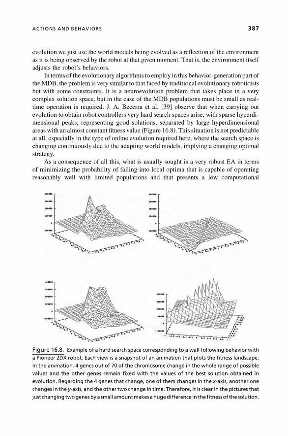
evolution we just use the world models being evolved as a reflection of the environment

as it is being observed by the robot at that given moment. That is, the environment itself

adjusts the robot’s behaviors.

In terms of the evolutionary algorithms to employ in this behavior-generation part of

theMDB, the problem is very similar to that faced by traditional evolutionary roboticists

but with some constraints. It is a neuroevolution problem that takes place in a very

complex solution space, but in the case of the MDB populations must be small as real-

time operation is required. J. A. Becerra et al. [39] observe that when carrying out

evolution to obtain robot controllers very hard search spaces arise, with sparse hyperdi-

mensional peaks, representing good solutions, separated by large hyperdimensional

areas with an almost constant fitness value (Figure 16.8). This situation is not predictable

at all, especially in the type of online evolution required here, where the search space is

changing continuously due to the adapting world models, implying a changing optimal

strategy.

As a consequence of all this, what is usually sought is a very robust EA in terms

of minimizing the probability of falling into local optima that is capable of operating

reasonably well with limited populations and that presents a low computational

Figure 16.8. Example of a hard search space corresponding to a wall following behavior with

a Pioneer 2DX robot. Each view is a snapshot of an animation that plots the fitness landscape.

In the animation, 4 genes out of 70 of the chromosome change in the whole range of possible

values and the other genes remain fixed with the values of the best solution obtained in

evolution. Regarding the 4 genes that change, one of them changes in the x-axis, another one

changes in the y-axis, and the other two change in time. Therefore, it is clear in the pictures that

just changing twogenesbya small amountmakesahugedifference in thefitnessof the solution.


complexity. The macroevolutionary algorithm (MA) [40], which is the algorithm

selected here, seems to be an appropriate choice [39]. The main difference between

MAs and other kinds of EAs is how selection formating is performed. For themajority of

EAs, more fitness means more probability of mating and transmitting information to the

next generation. In MAs, fitness plays a role together with distance between individuals

in order to determine who survives and, once an individual is tagged as a survivor, it has

the same probabilities of reproducing as any other survivor. The MA’s dynamics can be

summarized as follows:

1. An initial population is randomly generated. In MAs, the term species is used

instead of individuals in order to provide a better analogy with nature, although

in current implementations each species corresponds to a single individual.

2. The population is evaluated.

3. A survival coefficient is calculated for each species i as the sum of ( f(i)� f(j))/

d(i� j), where j is every other species, f the fitness function, and d the distance

in the search space. If that sum is positive, the species survives; otherwise, it

becomes extinct. That is, a species survives if its fitness is better than a weighted

average that takes into account the distance between species. Consequently,

a species can survivewith a relatively poor fitness value if it is far from the rest of

the species.

4. Each extinct species is substituted by another species that can be randomly

generated or derived froma combination of itself and a randomly chosen survivor

depending on the value of a t parameter. This parameter is usually set up so that

in the first generations most of the new species are random, and, in the last

generations, most of the new species are derived from combining extinct species

with survivors, going from almost pure exploration to almost pure exploitation as

generations evolve.

5. The population is evaluated again and the algorithm loops until a stopping

criterion (number of generations or a given fitness value) is reached.

This particular way of performing selection, taking into account distance in the

search space and maintaining a low evolutionary pressure, produces a niching effect in

the population; that is, individuals tend to organize themselves into clusters in the search

space simultaneously exploring different areas, which helps to avoid falling into local

optima. Finally, MAs also present a low computational complexity for low populations,

which is the case in online evolution.

16.5 SOME APPLICATION EXAMPLES

In this section, we are going to present some application examples. The objective is to

provide an indication of the possibilities of the different elements that go into the MDB.

Initially, an example is described where a complete behavior-based control architecture

is obtained for a Pioneer 2 DX robot in order to demonstrate the versatility and


capabilities of modulation-based architectures as a base for the action part of the global

cognitive mechanism. In fact, the complex controller obtained is an example of the

base controllers that can be inserted as initial material to be refined by the cognitive

mechanism when in real-time operation. After this, we describe an example where the

whole MDB cognitive mechanism is used, showing its ability to adapt and readapt to

different environments and/or tasks through a process of interacting with teachers.

16.5.1 Training a Modulation Architecture

The following example [41] illustrates the offline process for obtaining controllers with

the aim of showing how the behavior-based architecture used for the action part of the

cognitive mechanism obtains complex behaviors from combinations of simple modules

and modulation. The example shows many of the architecture components, including

both input and output modulation.

In this behavior, the robot has to catch a prey avoiding a predator. Prey and predator

are also mobile objects. The robot gains energy as it goes near the prey and loses energy

as it goes near the predator. There are two internal values that also affect the robot energy:

the energetic cost associated with each step and the anxiety level of the robot that makes

it lose energy (the higher the anxiety level, the higher the energy loss). The objective is to

catch the prey, maximizing energy. That means that if the energetic cost in each step or

the anxiety is very high, the robot should go straight to the prey, without worrying about

being near the predator. Otherwise, the robot should try to catch the prey while avoiding

the predator by a long distance.

The controller has 4 modules: 2 low-level modules (go straight to the prey and

escape straight from the predator), 1 actuator modulator (which modulates outputs of

the 2 low-level modules depending on distance to prey and predator and the energetic

cost associated with each step) and 1 sensor modulator (which modulates inputs of

the actuator modulator depending on anxiety). Figure 16.9 shows the controller

structure.

The ANN of the sensor modulator has 2 inputs, 2 hidden layers with 6 neurons each,

and 2 outputs. The ANN of the actuator modulator has 3 inputs (two of them modulated

by the sensormodulator), 2 hidden layers with 6 neurons each, and 2 outputs. To simplify

the problem, the only output of the low-level modules is the angular velocity (which will

be between �40�/sec and 40�/sec). Linear velocity is set to a fixed value (200mm/sec).

The prey escapes from the robot and the predator tries to get between the prey and the

robot. Amacroevolutionary algorithm [40]was used in every evolutionwith a very small

number of individuals (for instance, the sensor modulator’s evolution was performed

with a population of 100 individuals, during 100 generations, and each individual was

evaluated 200 times with a life of 300 steps).

The process was carried out as follows. First, the lowest-level modules were

obtained. Then, the actuator modulator was evolved and we had a behavior that allowed

the robot to catch the prey avoiding the predator by a distance that depends on the

energetic penalization for each step. Finally, a sensor modulator was obtained so that the

robot could take into account not only the energetic penalization but also its anxiety level

when deciding how far away the predator had to be.

SOME APPLICATION EXAMPLES 389

Figures 16.10 and 16.11 show some example runs. In the controllers resulting from

evolution, the actuator modulator regulates only the “escape from predator” module,

maintaining the modulation of the “go to prey” module constant. The sensor modulator

evolves in a similar way and it maintains the modulation of the sensor that indicates the

distance to the prey constant and modulates only the sensor that indicates the distance to

the predator. The constant modulation applied to the “distance to prey” sensor is in fact

a “0”, so the ANN corresponding to the actuator modulator can be pruned. This makes

Figure 16.9. Controller diagram.


sense; the actuator modulator activates the “go to prey”module by default and onlywhen

it is near the predator does it activate the “escape from predator” module. It is also really

interesting to see that the sensormodulator changes the actuatormodulator behavior only

when anxiety is higher than the amount of energy lost in each step; otherwise, the actuator

modulator already behaves correctly.

Figure 16.11. Example in the real robot.

Figure 16.10. Some examples of the global behavior in the simulator. Graphics represent

modulation levels. Dashed lines¼actuator modulator outputs; continuous lines¼ sensor mod-

ulator outputs.


16.5.2 Online Adaptation

The online learning capabilities of the MDB have been tested in different experiments

using real robots [42, 43]. The example we present here [44] employs the main features

of the architecture: real-time learning, real-time operation, physical agent operation, and

adaptive behavior. In order to emphasize the robustness of theMDB, we have carried out

the experiment using the Pioneer 2 robot and Sony’s AIBO robot.

The task the robotmust carry out is simple: Learn to obey the commands of a teacher

that, initially, guides the robot toward an object located in its neighbourhood. In

Figure 16.12, we show the experimental setup for both robots. In the case of the Pioneer

2 robot (left image of Figure 16.12), the object to reach is a black cylinder, and in the case

of the AIBO robot the object is a pink ball (right images of Figure 16.12). The Pioneer 2

robot is a wheeled robot that has a sonar sensor array around its body and a laptop placed

on its top platform. The laptop provides two more sensors, a microphone, and the

numerical keyboard, and the MDB runs on it. The AIBO robot is a doglike robot with

a larger range of sensors and actuators. In this example, we use the digital camera, the

microphones, and the speaker. The MDB is executed remotely on a PC and commu-

nicates with the robot through a wireless connection.

Figure 16.13 displays a schematic view of the current world and satisfaction models

(with their respective numbers of inputs and outputs) that arise in this experiment in a

given instant of time. The sensory meaning of the inputs and outputs of these models in

both physical agents is summarized in Table 16.1. In this example, we do not take into

account internal sensors in the agent and, consequently, internalmodels are not used. The

flowof the learning process is as follows: The teacher observes the relative position of the

robot with respect to the object and provides a command that guides it toward the object.

Figure 16.12. Left images show a sequence of real actions in the Pioneer 2 robot when the

teacher is present (top) and the robot uses the induced models (bottom). Middle and right

images correspond to the same situation, but in the case of the AIBO robot.


T A B L E 16.1. Inputs and Outputs Involved in the Models of the MDB for the Two PhysicalAgents Used in the Experiment

Pioneer 2 robot AIBO robot

Command (1 input) . Group of seven possible values

according to the seven musical

notes.

. Group of seven possible values

according to seven spoken

words: hard right, medium

right, right, straight, left, medi-

um left and hard left.. Provided by the teacher through

a musical keyboard.

. The teacher speaks directly.

. Sensed by the robot using the

microphone of the laptop.

. Sensed using the stereo micro-

phones of the robot.. Translated to a discrete numer-

ical range from �9 to 9.

. Speech recognition using

Sphinx software translated into

a discrete numerical range from

�9 to 9.

Action (1 input) . Group of seven possible ac-

tions: turn hard right, turn me-

dium right, turn right, follow

straight, turn left, turn medium

left and turn hard left that are

encoded with a discrete numer-

ical range from �9 to 9.

. Group of seven possible ac-

tions: turn hard right, turn me-

dium right, turn right, follow

straight, turn left, turn medium

left and turn hard left that are

encoded with a discrete numer-

ical range from �9 to 9.. The selected action is decoded

as linear and angular speed.

. The selected action is decoded

as linear speed, angular speed

and displacement.

Predicted human

feedback (1 output/

input)

. Discrete numerical range that

depends on the degree of ful-

fillment of a command from 0

(disobey) to 5 (obey).

. Group of five possible values

according to five spoken words:

well done, good dog, ok, pay

attention, bad dog.. Provided by the teacher directly

to theMDBusing the numerical

keyboard of the laptop.

. The teacher speaks directly

. Sensed using stereo micro-

phones of the robot.. Speech recognition using

Sphinx software translated into

a discrete numerical range from

0 to 5

Satisfaction

(1 output)

. Continuous numerical range

from 0 to 11 that is automati-

cally calculated after applying

an action. It depends on:

. Continuous numerical range

from 0 to 11 that is automati-

cally calculated after applying

an action. It depends on:

T The degree of fulfillment of a

command from 0 (disobey)

to 5 (obey).

T The degree of fulfillment of a

command from 0 (disobey)

to 5 (obey).

(continued)


Initially, the robot has no idea of what each command means in regard to the actions it

applies. After sensing the command, the robot acts and, depending on the degree of

obedience, the teacher provides a reward or a punishment as a pain or pleasure signal. The

motivation of the physical agent in this experiment is to maximize pleasure, which

basically means being rewarded by the teacher.

To carry out this task, the robot just needs to follow the commands of the teacher,

and a world model with that command as sensory input is obtained (top world model of

Figure 16.13) to select the action. From this point forward, we will call this model

communicationmodel. The satisfactionmodel (top satisfactionmodel of Figure 16.13) is

trivial as the satisfaction is directly related to the output of the communication model,

that is, the reward or punishment.

T A B L E 16.1 (Continued)

Pioneer 2 robot AIBO robot

T The distance increase from 0

(no increase) to 3 (max).

T The distance increase from 0

(no increase) to 3 (max).

T The angle with respect to the

object from 0 (back turned)

to 3 (robot frontally to the

object)

T The angle with respect to the

object from 0 (back turned)

to 3 (robot frontally to the

object).

Distance and angle

(2 outputs/inputs)


sonar array sensor.


images provided by the colour

camera.. Measured from the robot to the

black cylinder and encoded di-

rectly in cm and degrees.

. Colour segmentation process

and area calculation taken from

Tekkotsu software.. Encoded in cm and degrees.. Measured from the robot to the

pink ball.

Figure 16.13. Worldand satisfactionmodels involved in this examplewith their corresponding

sensory inputs and outputs.


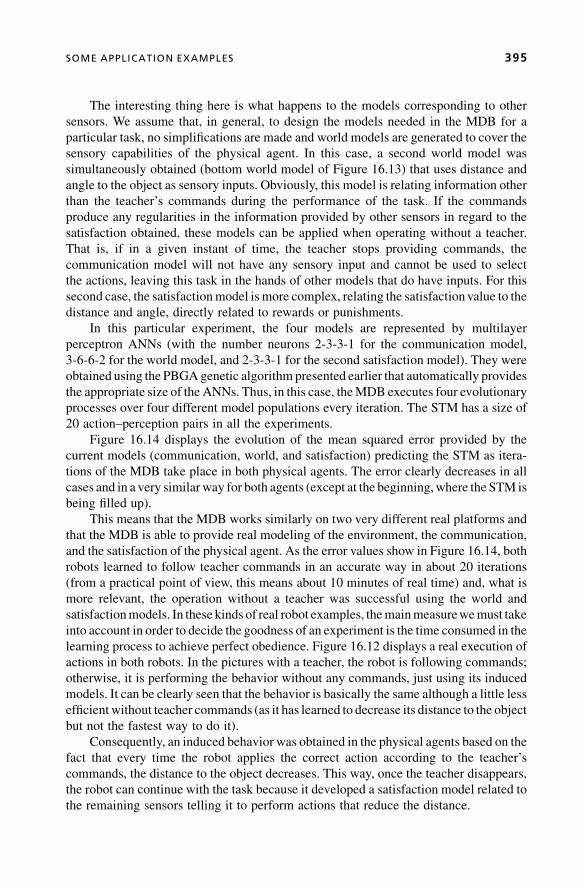
The interesting thing here is what happens to the models corresponding to other

sensors. We assume that, in general, to design the models needed in the MDB for a

particular task, no simplifications are made and world models are generated to cover the

sensory capabilities of the physical agent. In this case, a second world model was

simultaneously obtained (bottom world model of Figure 16.13) that uses distance and

angle to the object as sensory inputs. Obviously, this model is relating information other

than the teacher’s commands during the performance of the task. If the commands

produce any regularities in the information provided by other sensors in regard to the

satisfaction obtained, these models can be applied when operating without a teacher.

That is, if in a given instant of time, the teacher stops providing commands, the

communication model will not have any sensory input and cannot be used to select

the actions, leaving this task in the hands of other models that do have inputs. For this

second case, the satisfactionmodel is more complex, relating the satisfactionvalue to the

distance and angle, directly related to rewards or punishments.

In this particular experiment, the four models are represented by multilayer

perceptron ANNs (with the number neurons 2-3-3-1 for the communication model,

3-6-6-2 for the world model, and 2-3-3-1 for the second satisfaction model). They were

obtained using the PBGAgenetic algorithmpresented earlier that automatically provides

the appropriate size of the ANNs. Thus, in this case, theMDB executes four evolutionary

processes over four different model populations every iteration. The STM has a size of

20 action–perception pairs in all the experiments.

Figure 16.14 displays the evolution of the mean squared error provided by the

current models (communication, world, and satisfaction) predicting the STM as itera-

tions of the MDB take place in both physical agents. The error clearly decreases in all

cases and in a very similar way for both agents (except at the beginning,where the STM is

being filled up).

This means that the MDB works similarly on two very different real platforms and

that the MDB is able to provide real modeling of the environment, the communication,

and the satisfaction of the physical agent. As the error values show in Figure 16.14, both

robots learned to follow teacher commands in an accurate way in about 20 iterations

(from a practical point of view, this means about 10 minutes of real time) and, what is

more relevant, the operation without a teacher was successful using the world and

satisfactionmodels. In these kinds of real robot examples, themainmeasurewemust take

into account in order to decide the goodness of an experiment is the time consumed in the

learning process to achieve perfect obedience. Figure 16.12 displays a real execution of

actions in both robots. In the pictures with a teacher, the robot is following commands;

otherwise, it is performing the behavior without any commands, just using its induced

models. It can be clearly seen that the behavior is basically the same although a little less

efficientwithout teacher commands (as it has learned to decrease its distance to the object

but not the fastest way to do it).

Consequently, an induced behavior was obtained in the physical agents based on the

fact that every time the robot applies the correct action according to the teacher’s

commands, the distance to the object decreases. This way, once the teacher disappears,

the robot can continue with the task because it developed a satisfaction model related to

the remaining sensors telling it to perform actions that reduce the distance.


To show the adaptive capabilities of the MDB, in Figure 16.15 (left) we have

represented the evolution of the MSE provided by the current communication model

during 200 iterations for the example with the Pioneer 2 robot. In the first 70 iterations,

the teacher provides commands using the same encoding (language) applied in the

previous experiment. This encoding is not preestablished and we want the teacher to

make use of any correspondence it wants. From iteration 70 to iteration 160, another

teacher appears using a different language (different andmore complex relation between

musical notes for the Pioneer robot), and, finally, from iteration 160 to iteration 200, the

original teacher returns. As shown in the figure, in the first 70 iterations the error

Figure 16.14. Evolution of themean squared error of the current communicationmodel (top),

satisfaction model (middle), and world model (bottom) predicting the STM as iterations of the

MDB take place in the Pioneer 2 robot.

Figure 16.15. Evolution of the MSE provided by the current communication model (left) and

satisfactionmodel (right) predicting the STMas iterations of theMDB take place. The left graph

corresponds to a dynamic language and the right graph to a dynamic satisfaction.


decreases fast to a level (1.6%) that results in a very accurate prediction of the rewards.

Consequently, the robot successfully follows the commands of the teacher. When the

second teacher appears, the error level increases because the STM starts to store samples

of the new language and the previous models fail in the prediction. At this point, as

mentioned before, the LTMmanagement system detects this mixed situation (detects an

unstablemodel) and induces a change in the parameters of the STM replacement strategy

to a FIFO strategy. As displayed in Figure 16.15 (left), the increase in the value of the

error stops in about 10 iterations and, once the STM has been purged of samples from the

first teacher’s language, the error decreases again (1.3% at iteration 160). The error level

between iterations 70 and 160 is not as stable as in the first iterations. This happens

because the language used by the second teacher is more complex than the previous one

and, in addition, we must point out that the evolution graphs obtained from real robots

oscillate, in general, much more than in simulated experiments due to the broad range of

noise sources of the real environments. But the practical result is that about iteration 160

the robot follows the new teacher’s commands successfully again, adapting itself to

teacher characteristics. When the original teacher returns using the original language

(iteration 160 of Figure 16.15, left), the adaptation is very fast because the communi-

cation models stored in the LTM during the first iterations are introduced as seeds in the

evolutionary processes.

In Figure 16.15 (right) we have represented the evolution of theMSE for the current

satisfaction model in another execution of this second experiment. In this case, the

change occurs in the rewards provided by the teacher. From iterations 0 to 70, the teacher

rewards reaching the object and, as we can see in the graph, the error level is low (1.4%).

From iteration 70 to 160, the teacher changes its behavior and punishes reaching the

object, rewarding escaping from it. There is a clear increase of error level due to the

complexity of the new situation (high ambiguity of possible solutions, that is, there

are more directions of escaping than reaching the object). In iteration 160, the teacher

returns to the first behavior and, as expected, the error level decreases to the original

levels, quickly obtaining a successful adaptive behavior.

16.6 CONCLUSION

An approach based on the simultaneous use of a reactive modular ANN-based robot

architecture and amore deliberative lifelong-learningmechanism for autonomous robots

is presented here. These two approaches to the implementation of the complete control

system for an autonomous robot can be combined through the use of the reactive-based

modular structure as the action-generation part of an evolutionary-based cognitive

mechanism. The cognitive mechanism is in charge of obtaining and managing world

and internal models of the environments and the robot as well as satisfaction models,

which are used in its action-generation part to evolutionarily adapt the control structure

of the robot. One of the advantages of this approach is that some reactive architectures

can be roughly pretrained in simulation, as it is more efficient, and then introduced in

the real robot so that the cognitive mechanism can refine them to the level required by

the task.

CONCLUSION 397

This procedure greatly simplifies the task of the cognitive mechanism, as it does not

have to start from a clean slate and also facilitates the production of the reactive control

architectures, which do not have to be perfectly trained at the beginning. In fact, this

approach can be equated to the one used by nature, where a rough set of competencies are

preloaded in animal or human brains, which are then tuned to the particular environments

and circumstances each individual will face through adaptation by interacting with the

world.

Further work is necessary to assess the level of complexity that may be achieved

using these strategies, especially in terms of the size of the modular structures that are

manageable. But what is more important is to be able to elucidate a methodology that

allows for the automatic decomposition of large behaviors into coherent subparts that can

be reused by the cognitive mechanism when adapting. This is the main line we are now

working on.

16.7 REFERENCES

1. R. Pfeifer, J.C. Bongard, How the Body Shapes the Way We Think. MIT Press, 2006.

2. TheAmericanHeritage�Dictionary of the English Language, 4th ed.HoughtonMifflin, 2000.

3. L. M. Brasil, F. M. Azevedo, J. M. Barreto, M. Noirhomme-Fraiture, “Complexity and

Cognitive Computing,” IEA/AIE, Vol. 1, pp. 408–417, 1998.

4. S. Nolfi, S. & D. Floreano, Evolutionary Robotics: The Biology, Intelligence and Technology

of Self-Organizing Machines. Cambridge, MA: MIT, 2000.

5. R. A. Watson, S. G. Ficici, J. B. Pollack, “Embodied Evolution: Distributing an Evolutionary

Algorithm in a Population of Robots,”Robotics and Autonomous Systems, 39, pp 1–18, 2002.

6. U. Nehmzow, “Physically Embedded Genetic Algorithm Learning in Multi-Robot Scenarios:

The PEGA Algorithm.” Proc. 2nd Int. Workshop on Epigenetic Robotics: Modelling

Cognitive Development in Robotic Systems, 2002.

7. D. Floreano, J. Urzelai, “Evolution of Plastic Control Networks,” Autonomous Robots, 11,

pp. 311–317, 2001.

8. G. Hornby, S. Takamura, J. Yokono, O. Hanagata, T. Yamamoto, M. Fujita, “Evolving Robust

Gaits with AIBO.” IEEE Int. Conf. on Robotics and Automation, 2000, pp. 3040–3045.

9. D. Marocco, D. Floreano, “Active Vision and Feature Selection in Evolutionary Behavioural

Systems. From Animals to Animats: Proceedings of the Seventh Int. Conf on the Simulation

of Adaptive Behaviour (SAB’02), 2002, pp. 247–255.

10. M.Wilson, “Preston: A System for the Evaluation of Behaviour Sequences,” Interdisciplinary

Approaches to Robot Learning, In (Demmiris, J. and Birk, A.,eds.) Would Scientific, 24(9),

pp. 185–208, 2000.

11. J. Grefenstette, C. Ramsey, “An Approach to Anytime Learning.” Proc. 9th Int. Machine

Learning Conference, 1992, pp 189–195.

12. G. Parker, “Co-evolving Model Parameters for Anytime Learning in Evolutionary Robotics,”

Robotics and Autonomous Systems, 33, pp. 13–30, 2000.

13. J. Walker,“Experiments in Evolutionary Robotics: Investigating the Importance of Training

and Lifelong Adaptation by Evolution, PhD thesis, University of Wales, 2003.


14. J. Walker, S. Garret, M. Wilson, “Evolving Controllers for Real Robots: A Survey of the

Literature,” Adaptive Behavior, 11(3), pp. 179–203, 2006.

15. R. J. Duro, J. Santos, F. Bellas, A. Lamas, “On Line Darwinist Cognitive Mechanism for an

Artificial Organism.” Proc. Supplement Book SAB2000, 2000, pp. 215–224.

16. J. Changeux, P. Courrege, A. Danchin, “ATheory of the Epigenesis of Neural Networks by

Selective Stabilization of Synapses.” Proc. Nat. Acad. Sci. USA, 70, 1973, pp. 2974–2978.

17. M. Conrad, “Evolutionary Learning Circuits,” J. Theoretical Biology, 46, 1974.

18. G. Edelman,NeuralDarwinism: The Theory ofNeuronalGroup Selection. Basic Books, 1987,

pp. 167–188.

19. M. R. Genesereth, N. Nilsson, Logical Foundations of Artificial Intelligence. Morgan

Kauffman, 1987.

20. F. Bellas, R. J. Duro, “Multilevel Darwinist Brain in Robots: Initial Implementation.”

ICINCO2004 Proceedings Book, Vol. 2, 2004, pp. 25–32.

21. F. Bellas, R. J. Duro, “IntroducingLongTermMemory in anANN-BasedMultilevelDarwinist

Brain,” Lecture Notes in Computer Science, Vol. 2686, 2003, pp. 590–598.

22. F. Bellas, J. A. Becerra, R. J. Duro, “Construction of a Memory Management System in an

On-line Learning Mechanism.” ESANN 2006 Proceedings Book, 2006.

23. X. Yao, “Evolving Artificial Neural Networks.” Proc. IEEE, 87(9), 1999, 1423–1447.

24. K. Trojanowski, Z. Michalewicz, “Evolutionary Approach to Non-stationary Optimisation

Tasks.” Lecture Notes in Computer Science, Vol. 1609, 1999, pp. 538–546.

25. N. Mori, H. Kita, Y. Nishikawa, “Adaptation to a Changing Environment by Means of the

Feedback Thermodynamical Genetic Algorithm.” LNCS, Vol. 1498, pp. 149–158, 1998.

26. D. Dasgupta, D. R. MacGregor, “Nonstationary Function Optimization Using the Structured

Genetic Algorithm.” Proc. Parallel Problem Solving from Nature 2, 1992, pp. 145–154.

27. C. Ryan, J. J. Collins, D. Wallin, “Non-stationary Function Optimization Using Polygenic

Inheritance.” Lecture Notes in Computer Science, Vol. 2724, pp. 1320–1331, 2003.

28. J. Eggermont, T. Lenaerts, “Non-stationary Function Optimization Using Evolutionary

Algorithms with a Case-Based Memory,” Technical Report TR 2001-11, 2001.

29. T. D’Silva, R. Janik, M. Chrien, K. Stanley, R. Miikkulainen, “Retaining Learned Behavior

During Real-Time Neuroevolution.” Proc. AIIDE 2005, 2005.

30. H. G. Cobb,“An Investigation into the Use of Hypermutation as an Adaptive Operator in

Genetic Algorithms Having Continuous, Time-Dependent Nonstationary Environments,”

NRL Memorandum Report 6760, pp. 523–529, 1990.

31. D. E. Moriarty,“Symbiotic Evolution of Neural Networks in Sequential Decision Tasks,”

PhD Thesis, University of Texas at Austin, Tech. Rep. UT-AI97-257, 1997.

32. F. Gomez, D. Burger, R. Miikkulainen, “A Neuroevolution Method for Dynamic Resource

Allocation on a Chip Multiprocessor.” Proc. Int. Joint Conf. on Neural Networks, 2001.

33. K. O. Stanley, R. Miikkulainen, “Evolving Neural Networks through Augmenting

Topologies,” Evolutionary Computation, 10, pp. 99–127, 2002.

34. D. Dasgupta, D. McGregor, “Designing Application-Specific Neural Networks Using the

Structured Genetic Algorithm.” Proc. COGANN-92, 1992, pp. 87–96.

35. F. Bellas, R. J. Duro, “Modelling theWorldwith StatiscallyNeutral PBGAs: Enhancement and

RealApplications.”Proc. 9th Int. Conf. onNeural InformationProcessing, Vol. 1, 2002, IEEE

Press, pp. 2093–2098.

REFERENCES 399

36. R. J. Duro, J. A. Becerra, J. Santos, “Behavior Reuse and Virtual Sensors in the Evolution of

Complex Behavior Architectures,” Theory in Biosciences, Vol. 120, pp. 188–206, 2001.

37. N. Jakobi, P. Husbands, I. Harvey, “Noise and the Reality Gap: The Use of Simulation in

Evolutionary Robotics,” Lecture Notes in Artificial Intelligence, Vol. 929, pp. 704–720, 1995.

38. J. Santos, R. J. Duro, J. A. Becerra, J. L. Crespo, F. Bellas, “Considerations in the Application

of Evolution to the Generation of Robot Controllers,” Information Sciences, Vol. 133,

pp. 127–148, 2001.

39. J. A. Becerra, J. Santos, R. J. Duro, “MA vs. GA in Low Population Evolutionary Processes

with Mostly Flat Fitness Landscapes.” Proc. 6th Joint Conf. on Information Sciences, 2002,

pp. 626–630.

40. J. Mar�ın, R.V. Sol�e, “Macroevolutionary Algorithms: ANewOptimizationMethod on Fitness

Landscapes,” IEEE Trans. on Evolutionary Computation, Vol. 3, No. 4, pp. 272–286, 1999.

41. J. A. Becerra, F. Bellas, J. Santos, R. J. Duro, “Complex Behaviours through Modulation in

Autonomous Robot Control,” LNCS 3512, pp. 717–724, 2005.

42. F. Bellas, A. Lamas, R. J. Duro, “Adaptive Behavior through a Darwinist Machine,” Lecture

Notes on Artificial Intelligence, 2159, pp 86–89, 2001.

43. F. Bellas, R. J. Duro, “Multilevel Darwinist Brain in Robots: Initial Implementation.”

ICINCO2004 Proceedings Book, Vol. 2, 2004, pp. 25–32.

44. F. Bellas, J. A. Becerra, R. J. Duro, “Induced Behaviour in a Real Agent Using the Multilevel

Darwinist Brain,” Lecture Notes in Computer Science, Vol. 3562, pp. 425–434, 2005.


17

APPLICATIONS OF EVOLVINGINTELLIGENT SYSTEMS TO OIL

AND GAS INDUSTRYJos�e Macıas-Hern�andez, Plamen Angelov

17.1 BACKGROUND

The oil and gas (O&G) industry has a variety of characteristics that make it suitable for

application of evolving intelligent systems (EISs). One can summarize these as:

. The need for constant product monitoring

. Low margin and high throughput

. A regulated market for the products and a free market for the crude

. High process complexity

. Expensive process investment

. High number of process variables

. High number of process products

The rawmaterial for refineries is crude oil. There are avast variety of crudeswith different

properties that will give different cuts and yields when processing. The price of crude

depends on several factors, ranging from its intrinsic chemical properties to political

stability in the country of supply and short- and long-termmarket behavior. The crude oil

purchase department has to balance spot market and long-term contracts to maintain a


and Nikola Kasabov


stable crude supply to their refineries. Yields in crude have to fit refineries’ complexity to

balance the local consumption. Any violation of the balance is normally undesirable.

Oil refining activities are characterized by low margin and high throughput. The

international energy market is free, but the local market is normally highly regulated.

Therefore, lowering production costs is the best option for refineries to survive; they have

to produce as many intermediate materials as possible. Importing intermediate compo-

nents is not optimal. For a process industry with such characteristics, online process

monitoring and control is very important.

The processes in an oil refinery generate huge volumes and streams of data that are

routinely stored in huge databases. The operator of a typical distributed control system

(DCS) in a complex contemporary oil refinery controls andmonitors several process units

andhas responsibility formore than 400valves!A typical oil refinery database can contain

as many as 10,000–12,000 continuous data points. Laboratory samples are routinely

analyzed andmore than 2000 characteristics are reported every day. The process operators

continuously (in real time) make decisions based on previous experience to drive the

process toward targets. With evolving intelligent sensors, this process can be automated.

An oil refinery usually produces a very high number of products, which ranges from

light hydrocarbons to heavy fuels. There are a high number of legal specifications that

impact the process economics. It is normal practice to blend several intermediate

products and recipes in various combinations in order to produce different final products.

All of these combinations have to meet legal specifications. The balance between

specifications and product components gives the degrees of freedom and emphasizes the

need for online monitoring of the quality of the products.

17.2 APPLICATION OPPORTUNITIES

An oil refinery is a complex industrial installation from the point of view that the number

of interconnected processes is large, but also from the point of view of the work

organization (White, 2001, 2003). In general, different implementations of evolving

intelligent systems (EISs) can be applied in different departments of a typical oil refinery.

Table 17.1 shows the possible areas and problems that can be addressed by different

T A B L E 17.1. Potential Application Areas for EIS in O&G Industry

Departments/Areas Application Type

Operations Alarm monitoring, operator advisory, emergency management

Price Prediction Regression and time-series prediction models (e.g., eTSþ )

Process Engineering Process diagnostics (e.g., eClusteringþ )

Information Systems Mining data streams (e.g., eTSþ ) (Angelov & Filev, 2004;

Angelov & Zhou, 2006; see also Chapter 2)

Predictive Maintenance Machine health monitoring and prognostics (e.g., eClustering

and eTS) (Filev & Tseng, 2006)

Control Engineering eControl, guided rule-base adaptation (Filev et al., 2000)

Soft Sensors eSensor (Angelov et al., 2008)

402 APPLICATIONS OF EVOLVING INTELLIGENT SYSTEMS TO OIL AND GAS INDUSTRY

realizations of EISs. The majority of these departments can be found in any complex

industrial system. Therefore, some of the general ideas shown in the table can be applied

to any industrial plant.

17.2.1 Planning and Scheduling

The complexity and the opportunities to applyEIS to oil refineries beginwith the purchase

of crude oil. As we have shown, there are tradeoffs among quality, yields, spot and long-

term deals, and international policies that impact refinery economics. The purchase of oil

(amount and quality) and the products that are being produced have to balance themarket

demands. Planning and scheduling departments have to deal with this problem. There is,

therefore, an opportunity to have a complex nonlinear, nonstationarymodel that takes into

account all of this highly uncertain information (ERTC, 2004;Goel & Prashant, 1999).

Some companies have reported commercial products that address these problems (e.g.,

Aspentech�, GenSym�, but clearly there is an opportunity formore advanced solutions in

this area that take the dynamics of the economic processes into account.

17.2.2 Operations

Complex industrial plants running different types of crude assays are difficult to analyze

in real time. Operations and process engineering departments have to deal with short-

term process troubleshooting, security, and quality management. Process operators have

to deal with problems associated with the process security, stability, quality, and

optimization targets of the plant. Therefore, there are various opportunities to apply

EISs to the field of process operations:

Operator advisory applications. It is required to help operators in the real-time

decision-making process aiming to maintain security, stability, and process

optimization (Mac�ıas-Hern�andez, 2001).

Alarm monitoring and rationalization. The main goal is to detect and identify

abnormal behavior. Tools that can be useful and efficient for online implemen-

tation include eClusteringþ , eTSþ (Angelov, 2006; see also Chapter 2).

Emergency manager. This is related to the previous item, but here the goal is to

help the operator to manage emergency situations.

17.2.3 Process Engineering

The responsibilities of the process engineering department are process design and

troubleshooting. Traditionally, process engineers use steady-state simulators to create

virtual plants to calculate yields, and so on. Neural networks and neuro-fuzzy models

provide an efficient alternative for a rigorous steady-state simulation (Barsamian &

Mac�ıas, 1998). Process troubleshooting is related to short-term analysis of the process

behavior.Most instrument providers havevery efficient software for basic instrumentation

troubleshooting. Process diagnostics, however, is a more complex problem. Currently,

APPLICATION OPPORTUNITIES 403

there is no commercial software to accomplish this task in an automatic fashion. A

possible solution might be the use of eClustering and eTS (Filev & Tseng, 2006).

17.2.4 Maintenance

Predictive maintenance is a key activity to reduce total maintenance cost. The challenge

is to detect when and how equipment is going to fail based on vibration analysis, mean

time between failures (MTBF), process variables, corrosion indicators, and so forth. This

is a very good opportunity to apply anEIS.An early sensor failure detection is, in general,

an open problem. There are successful applications where this is the case, such as

vibration analysis, but cross-correlation between process operating data and equipment

failure is not done in an automatic fashion. eClustering and eTS are very promising tools

for this problem (Filev & Tseng, 2006).

17.2.5 Process Control

Control engineering has several general challenges:

Software sensors. There are a lot of successful applications of soft sensors

(Barsamian et al., 1998; Bhat et al., 2003; Fortuna et al., 2007; Kordon and

Smits, 2001; Rallo et al., 2004; Smits et al., 2006, etc.). Most of them, however,

are based on offline, black-box-type models. These are not able to recalibrate, or

to provide an insight to the process (are not transparent), and do not take into

account environmental dynamics and internal changes in the plant (different

operating modes, ageing, contamination), and so on. As a result, the life-cycle

costs of conventional soft sensors are high.

Dynamicmodel identification.Classical control theory provides a solid theoreticalbasis for linear cases and a limited number of nonlinear ones. Data mining is

suitable for offline cases, and dynamic model identification is a very promising

area; but for general nonlinear cases, there are practically no ready solutions apart

from EISs.

Detecting drift and shift. in the data pattern in streaming data (Angelov &

Zhou, 2008a).

Hybrid controllers. (multivariable predictive control [MPC] þ fuzzy techniques).

MPC tools are mature; however, their utilization depends on a properly designed

controller and the selection of variables (Camacho & Bordons, 1999). The first

part is usually done in practice using the Lyapunov theory, or linear matrix

inequalities (LMI) by the design engineer. Variables selection is an important task

that can be done automatically.

17.2.6 Information Systems

Modern DCSs have huge volumes of data that are processed and stored by sophisticated

information systems. It is common to find, including in the DCS, high-resolution history


(snap values) with a limited timeframe. In the majority of cases, there is low-resolution

history (average data values) with probably several years of data history. All this data

feeds several corporate applications, such as data reconciliation packages, oil move-

ments, product balance, and so forth. The results of these applications permit monitoring

of the overall refinery performance and support the planning, accounting, and operations

departments.

However, the data is usually highly correlated, so the useful information that is

contained there is much less than the overall amount of information stored and

collected online. Moreover, the successive events encountered in the plant are not

specified in the database, so sometimes the diagnosis of a problem in the operation or

in the performance of the plant is very difficult. Therefore, this volume of data alone in

the majority of cases is not useful for a deep understanding of the process unit. Because

of this, the diagnosis of any plant operation problem is madewhen it is fully developed,

and with the use of raw data and the immediate knowledge of the operations of

the plant.

The main characteristic of the database is to have a lot of variables but a short

operatingwindow. Because there are different crude types, it is highly noisy. Care should

be taken to design models with high information content and robustness.

It is clearly necessary to have more tools to manipulate the data and convert it to

information in industrial processes so that it can be used to help in diagnosis and process

follow-up. For instance, information can be used to help operators, and aid in diagnosis

and better control of processes. Process engineers can improve process performance and

planners can select the best feed for each process and plant status. Control engineers can

design more robust advanced control applications and solve unconventional process

control problems.

To do this effectively, advanced tools for mining data streams are required (e.g., the

eTSþ approach described in Chapter 2). Figure 17.1 shows a summary of functionality,

decision levels, and timeframe data.

Scope of ApplicationLevel of Decision

Sensors

Single-Loop

Plant Area

Operating Unit

Overall Plant

Plant Departments

Strategic Decisions

Logistics and Planning

Supervisory Control

Plant

Regulatory

Control

Week/Month

Seconds/Minutes

Days/Week

Hours/Shift

Seconds/Minutes

Years

OPC

DCS

Figure 17.1. Information and decision-making pyramid showing decision levels and applica-

tion areas for the O&G industry. (DCS denotes digital control system; OPC denotes OLE for

process control.)

APPLICATION OPPORTUNITIES 405

17.3 REFINERY

An oil refinery consists of an industrial installation where crude oil is separated on its

fraction, and then those fractions are treated to produce other fine products. The

commercial products are blended mixtures of intermediate refinery products to meet

legal specifications (See Figure 17.2).

In this section, the refining process will be briefly described, emphasizing the

opportunities for application of EISs to improve the quality of the products and the

efficiency.

17.3.1 Raw Material

The crude qualities (apart from the yield of each fraction) that are present and have the

most impact on refinery economics are sulfur, density, parafinicity or pour point, carbon

residue, salt content, nitrogen content, and metals. Sulfur impacts the refinery eco-

nomics because hydro-treating is required for most of the petroleum fractions. Sour

crudes are cheaper than sweet crudes. Low-density crudes correlate to lighter crudes and

produce a lower amount of fuel oil, which is one of the cheapest fractions. Upgrading

naphtha to gasoline requires the increase of aromaticity of the fraction and that uses

energy and requires processing. Therefore, lower parafinicity crudes are cheaper. The

carbon residue is related to asphalt content, which is the cheapest fraction. Salt produces

corrosion in the process units. Themore salts it contains, the cheaper the crude. Nitrogen

and sulphur are catalyst poisoning and should be removed. Metals produce catalyst

poisoning and severe deactivation.

Isomerization

Hydro-treating Reforming

Vapor Recovery

Catalytic Cracking

Alkylation

Aromatic Reduction

Propane Deasphalter

Vis-breaker

Dewaxing

Hydro Cracking

Delayed Coker

Trea

tin

g a

nd

Ble

nd

ing

CrudeUnit

Stabilizer Section

CrudeUnitAtm.

Tower Section

CrudeUnit

Vacuum Section

CRUDE

LPG and GAS

Straight Run Gasoline

Naphtha

Middle Distillates

GasolineHeavy Atmospheric Gas Oil

Vac. Gas Oil

LCO

Lube Base Stocks

Gasoline, Naphtha and Middle DistillatesFuel Oil

Asphalt

Gasoline, Naphtha and Middle Distillates

Lube Oils

Gas

Waxes

Gasoline, Naphtha and Middle Distillates

COKE

Asphalts

Greases

Lube Oils

Heating Oils

Diesels

Aviation Fuels

Solvents

Premium Gasoline

Regular Gasoline

LPG

Refinery Fuel Gas

Industrial Fuels

Refinery Fuel Oil

Hydro-treating

Figure 17.2. Typical complex refinery flowsheet.


17.3.2 Process Units

Opportunities for the use of EIS technology in process units can be analyzed from the

point of view of quality monitoring and control. Because there are numerous processes,

we select only the most typical ones. The same ideas can be extrapolated to others. The

principal operations required in a typical refinery are discussed in the following

subsections.

17.3.2.1 Distillation. Process Description. It is the first unit in the flowsheet,

and its mission is to separate by distillation the different crude fractions by means of

boiling the crude and condensing (see Figure 17.3). Steam is added to improve the

separation. The fractions obtained normally are:

. Naphtha

. Kerosene

. Gas oil

. Fuel oil

If there is a vacuum tower, it will be fed with fuel oil from the main distillation tower and

this second distillation will produce vacuum gas oil and asphalt.

Process Key Variables. The key operating variables are:

. Furnace temperature

. Top reflux

WATER

REFLUX DRUM

LPG RECOVERY

CW

CRUDE

KNO

GOL

HEATER

STEAMSALT WATER

DESALTER

STEAM

CRUDE

FUEL OIL

GASOIL

KNO

NAPHTHA

STEAM

Figure 17.3. Crude distillation unit.

REFINERY 407

. Side tower heat removal

. Process side-stream flows

These variables produce different ranges of side-stream qualities. It is important these

qualities are right because there are no further opportunities to correct them.

Opportunities for EIS. The opportunities to apply an EIS are mainly in soft

sensors—for example, soft analyzers for side-stream cut-point calculations. These are

used instead of real distillation analyzers, which are expensive and highly maintenance

dependent. Currently used technologies are offline neural networks (NNs), but there are

successful applications using partial least squares, PLS and bias update (Mac�ıas, 1998).The latter is especially important for close-loop soft control due to its robustness. There

are other soft sensors required for tower-loading calculations.

. Crude switch. Each time the process unit changes crude, the unit should be

adjusted to maintain qualities. The transient response of the unit is different from

normal operation. Therefore, the transient should be detected and corrected in

advance so the time-off specification is reduced to a minimum. Detection of the

transient is not precisely specified and represents an open problem.

. Feed properties and operation conditions. Crude tower behaviors differ from

one crude type to another. The unit should be adjusted to the newoptimumsettings.

This is typically accomplished by analyzing the process database to find the best

operating conditions of the unit or using case-based reasoning. An alternative

would be to use an EIS for online update to the new conditions. A good example of

an EIS is the guided rule-base initialization applied to advanced manufacturing

(Filev et al., 2000).

A case study based on development of evolving intelligent sensors (eSensor) for

estimation of different quality parameters of the distillation process will be described in

more detail in section 17.4. Four different quality parameters will be of interest:

1. Thn,�C: temperature of the heavy naphthawhen it evaporates 95% liquid volume,

ASTM D86-04b

2. Tk,�C: temperature of the kerosene when it evaporates 95% liquid volume,

ASTM D86-04b

3. A,�C: Abel inflammability analysis of the kerosene

4. Tgol,�C: temperature of the gas oilwhen it evaporates 85% liquid volume,ASTM

D86-04b

The inputs of interest for predicting Thn are (Maci�as et al., 2003):

. p,kg/cm2g: pressure of the tower

. P,%: amount of the product taking off

. d,g/l: density of the crude


. Tco,�C: temperature of the column overhead

. Tne,�C: temperature of the naphtha extraction

The inputs of highest relevance for predicting Tk are (Maci�as et al., 2003):

. p,kg/cm2: pressure of the tower

. P,%: amount of product taking off



. SGK,kg/h: steam introduced in GOL stripper

. Tke,�C: temperature of the kerosene extraction


The inputs suggested for predicting the Abel inflammability index of the Kero-

sene are:


. P,%: amount of the product taking off




. SK,kg/h: steam introduced in kerosene stripper

The inputs selected for predicting the temperature of the GOL when it evaporates 85%

liquid volume are (Maci�as et al., 2003):


. P,%: amount of product taking off



. SG,kg/h: steam introduced in GOL stripper

. Tke,�C: temperature of the kerosene extraction


17.3.2.2 Hydro-treating. Process Description. Hydro-treaters process a feed

in the presence of hydrogen to convert sulfur combined to SH2. This componentwill have

to be removed in a stripper tower. This unit is used for treatment of naphtha, kerosene, and

gas oil (Figure 17.4). This reaction takes place in the presence of a catalyst at high

temperature and pressure. Metals are not allowed because they destroy the catalyst.

During the process, coke is formed due to cracking. Hydrogen is used to minimize

cracking in the reactor.

REFINERY 409

ProcessKeyVariables. Thekeyvariablesthatcontroltheseverityofthereactionare:

. Reactor temperature

. Spatial velocity

Recycling hydrogen controls the length of the run. To remove the SH2 dissolved in the

reactor, effluent vapor or bottom temperature in the stripper are controlled.

Opportunities. Reactor models are only approximated and should be adjusted to

process variables. Also, the activity of the catalyst changes and therefore a long-term

adjustment should be made. This calls for evolving recalibrating models. The difficulty

arises due to the fact that the feed is not perfectly characterized. This requires the use of

fuzzy sets. eTSþ is thus perfectly placed to be used as a backbone technology for the

development of advanced evolving soft sensors (eSensors) to address this problem.

17.3.2.3 Reforming. Process Description. Reforming is a catalytic process

designed to increase the aromatic and isoparafinic content of naphtha, producing

high-octane gasoline (Figure 17.5). This process takes place in several reactors in

series, using hydrogen to protect the catalyst. Hydrogen is produced as well in the unit

due to dehydrogenation reactions. Some cracking takes place, producing liquefied

petroleum gas (LPG) and refinery gas.

Process Key Variables. Temperature and spatial velocity are again the key

variables. A post-fractionation control separates the LPG and gas from the reformed

naphtha. The operation variables in that tower are the reflux ratio and the boil-up

temperature. Control variables normally are the octane number and the Reid vapor

pressure of the reformed naphtha.

Opportunities. An EIS can be derived to model the operation of the unit to

accomplish octane number and yields. Such a model should take into account the

Hydrogen RecycleHydrogen Makeup

C3 and lighter to H2S removal

CW

Reactor

Heater

CW

Feed

Hydrogen Separator Stripper

Desulfurized Product

Steam or Hot Oil

Sour Water

Figure 17.4. Hydro-treating unit.


deactivation process of the catalyst. Ideally, it should be able to recalibrate and retrain

automatically. It is not usual to have octane analyzer at the bottom of the fractionation, so

an EIS-based soft sensor can be designed based on operating conditions and type of feed.

This latter characteristic should be derived upstream in crude and naphtha hydro-treating

units.

17.3.2.4 Catalytic Cracking. Process Description. Fluid catalytic cracking is a

technology to break the gas oil into gasoline and lighter fractions (Figure 17.6). Due to

the very high speed of deactivation of the catalyst because of the severe operating

conditions, the regeneration process takes place simultaneously in a second regenerator

reactor. The catalyst moves from the reactor to the regenerator. The catalyst coke is

burned in the regenerator using air.

Figure 17.6. Catalytic cracking unit.

CW

CW

Hydrogen Separator

Steam or Hot Oil

Gas

Feed

Hydrogen Recycle

CWHeaters and Reactors

Reformated Naphtha

Figure 17.5. Catalytic reforming unit.

REFINERY 411

Process Key Variables. With the fixed type of feedstock, the major operating

variables that affect the conversion and product distribution are:

. Cracking temperature

. Catalyst-to-feed ratio

. Space velocity

. Type of catalyst

. Recycle ratio

To increase the conversion, we must increase reaction temperature, catalyst-to-feed

ratio, catalyst activity, and reaction time. The limitations come from the limit on burning

activity, limit in the air compressor, and the limitation of temperature in the regenerator.

Sometimes, oxygen is added to increase the burning capability of the regenerator reactor.

Opportunities.This is a strong case for EIS-based soft analyzers to calculate octane

number of the gasoline and product distribution. There is also a case for hybridmodels to

simulate the reaction and regeneration sections in a mixed approach to rigorous

simulation of the main fractionation to balance catalyst activity with ageing and severity

using, for instance, eTSþ . A difficult and challenging task is to detect early different

types of feed to facilitate a faster move to unit limits. There is a large scope to address this

using techniques such as eClusteringþ and age of the clusters.

17.3.2.5 Thermal Cracking. Process Description. Vis-breaking is a type of

thermal cracking that reduces the viscosity of a heavier feed to a lower-viscosity fuel by

means of breaking higher-molecular-weight molecules into gasoline, kerosene, gas oil,

and lower-viscosity fuel (Figure 17.7). The reaction takes place by temperature and space

STEAM

Gas

Gasoline

Water

Gas Oil

Fractionator

STEAM

Fuel Oil

SoakerFurnace

Atmospheric Fuel Oil

Figure 17.7. Vis-breaking of soaker type.


velocity in the furnace (coil vis-breakers) or a soaker drum (soaker vis-breaker). The first

one gets product yields by temperature, the second one by the space velocity. As a result,

soaker drum vis-breakers get longer run times than coil vis-breakers. The reactor effluent

is separated in fractions in fractionation and stabilizer towers. Run length is controlled by

coke deposition in the furnace, which limits the skin temperature.

Process Key Variables. The key process variables are the temperature and the

spatial velocity. There are other operating variables in the fractionation, such as steam,

reflux ratio, and heat distribution in the tower. The key variable is the stability of the fuel

oil bottoms of the fractionation. A major practical obstacle is the lack of analyzers for

stability.Manipulating the extraction side streams and the stripping steam should control

side-stream cut point. Some types of feed are more sensitive to coke lay-down than

others. Prediction of coke lay-down is important to optimize the run length.

Opportunities.There are great opportunities for EIS-based soft analyzers to predict

the stability of the cracked fuel oil, that is the key variable for profit in this process unit.

There is also an opportunity for a flexible vis-breaking reaction model possibly mixed

with rigorous steady-state tower simulation into a hybrid model. There is also a need to

characterize the cracking ability and stability with the aim to predict coke lay-down and

run length. This information can be used to manipulate operating variables when

switching from one feed type to another.

17.4 CASE STUDY: eSENSOR FOR QUALITY-OF-PRODUCT ONLINEMONITORING

In this section, a particular application of a soft sensor that is based on eTSþ , called

eSensor, will be presented for monitoring the quality of oil products online. Soft sensors

and eSensors in particular can contribute to increasing the level of automation and to

bringing down life-cycle costs of the exploitation of these sensors in the O&G industry.

Due to the extremely high throughput of the oil refinery process, any improvement in

product quality has significant impact on the cost and the final profit. The process is

complex; a large number of internal variables and many process products (outputs) are

involved. Operational environment may also affect the process. Due to the complexity

and high setting requirement, the data is usually collected on a daily basis. Considering

the high throughput, interrupts of the process are very costly. The continuous running of

such a process is very important. As described in the previous sections, the crude oil

distillation tower is the first and most important part of the oil refinery. Crude oil is

separated into several major cuts (contents) in the distillation tower according to their

density and temperature after being heated. These contents are extracted from the

distillation tower with lateral pipes and in the consequent processes are refined and

blended into gasoline, gas oil, and other commercial products.

The specification for distillation usually is very strict (Macias et al., 2003). The

quality of this initial separation of crude oil has a fundamental impact on the efficiency of

the later refining process. The 95% ASTM distillation curve (Macias et al., 2003)

specifies the relation between the distillated products and the temperature of the

corresponding side vapor stream from the tower (see Figure 17.3). Normally, the

CASE STUDY: eSENSOR FOR QUALITY-OF-PRODUCT ONLINE MONITORING 413

products that come from the top end of the distillation tower, have a lower boiling point

and higher quality and price. The economic goal of the distillation is to obtain the

maximum amount of higher-quality product (Maci�as et al. 2003).Based on the analysis of the samples andmeasurements, the operators can adjust the

equipment settings and input crude oil, aiming to reduce the deviation of the product

quality from the specification. Conventionally, samples are taken for laboratory analysis,

which is a costly and slow manual procedure. Another problem with the laboratory

analysis is that there are a lot of errors due to the different sampling method, the

arbitrarily determined error compensation, and so on. Another issue is that the laboratory

analysis usually has hourly or daily delay,which leads to additional error. Attempts to use

soft sensors to predict the quality of the crude oil distillation started some 20 years ago

using principal component analysis (PCA) (Keinosuke, 1990; Li et al., 2000), partial

least squares (PLS) (Kaspar, 1993), and genetic programming (Kordon et al., 2003;

Smits et al., 2006). More recently, with the development of more advanced modeling

techniques, such as neural networks (Rodriguez et al., 1997) and support vector

machines (SVMs) (Yan et al., 2004), a significant improvement in prediction accuracy

has been achieved. The practice shows that this kind of soft sensor is able to maintain

acceptable prediction accuracy when the process is stable.

However, in real industrial plants, it is usually not possible tomaintain the consistent

stability of the processes. Once the shifts and drifts take place in the data pattern that

describes the process, the pretrained models have to be retrained (soft sensors have to be

recalibrated). Therefore, there is a clear demand for online adaptive/evolvingmodels that

are able to cope with the concept of shifts and drifts in the dynamic process, and to self-

calibrate and adapt to the dynamic changes in the environment and the plant (EC, 2007;

Qin et al., 1997). Applying evolving intelligent models such as eTSþ will significantly

increase the level of automation of the refining process.

17.4.1 Description of the Case Study

The plant used for this case study is a crude distillation installationwith a design capacity

of 80,000 bbl/d of crude oil from the Middle East (Maci�as et al., 2003). It has 47 valve

trays with a diameter of 5.2m in its top section and 2.4m at the bottom section. The tower

has two cold pumps (kerosene oil [KNO] and gas oil [GOL]) and a hot pump.

From the top to the bottom, the six side streams are (Maci�as et al., 2003):

1. Heavy naphtha (HN)

2. Kerosene (KN)

3. Light gas oil (LGO)

4. Medium gas oil (MGO)

5. Heavy gas oil (HGO)

6. Bottom product, atmospheric residue (RES)

The data for online training and validating of the proposed evolving intelligent sensor are

the instrument readings and the output data, including the information on emergencies,


shutdowns, process and instrument malfunction, and so on. They are taken on a daily

basis. In order to test the performance of the proposed evolving intelligent sensor in

conditions close to the reality, the raw data has not been filtered out. The inputs for the

modeling are:

. Temperatures

. Flow rates

. Pressures of the tower

. Stream injections

. Unit throughput

. Crude density

Four different eSensors were designed, one for each of the variables of interest to be

estimated (see section 17.3.2.1). Note that alternatively one can design also a single

eSensor with four outputs using the property of eTSþ to be suitable for multi-input-

multi-output (MIMO) problems (Angelov et al., 2004). In this study we have developed

four separate eSensors using all availablemeasurable variables and letting eSensor select

themost suitable input variables online. Note that the tests were performed in a simulated

online mode, but real-life experiments are currently taking place at the CPESA.

In Figure 17.8, eSensor predicts the value of Thn (respectively the other quality

parameters) based on themeasured online (by hard sensors) temperatures, pressures, and

so forth. The input variables selection block automatically reduces the number of input

Figure 17.8. Schematic representation of the proposed eSensor for Thn.


variables based on their contribution as described inChapters 2 and 14 (section 14.5) into

a smaller number of inputs that contribute most to the prediction. From time to time,

recalibration of eSensor is needed (the right-hand side of Figure 17.8). This is done

automatically without retraining of the model in terms of a change of the structure, but

rather as a smooth correction. This process (recalibration) also does not require human

involvement and expertise and thus reduces the maintenance and life-cycle costs

significantly.

The proposed evolving inferential sensors have two main modes of operation:

(1) prediction or estimation, and (2) recalibration (self-learning). Initially, the second

mode is active to build (evolve) the structure (fuzzy rule base) of the sensor automatically

online.This requires a relatively small number of training samples.

The experiment includes a simulated online mode of operation with initial sensor

design stage (learning the rule base) based on a certain limited number of samples (90

samples that correspond to threemonths ofwork of the refinery) and a recalibration phase

of 60 samples (two months of operation of the refinery) starting at sample 271 (that is,

after half a year of predictionwith a fixedmodel). Thewhole data set consists of 447 daily

measurements taken atCEPSAOilRefinery, SantaCruz deTenerife, a fewyears ago. The

results compare three modes:

1. A limited period of learning (90 samples) followed by fixing the structure of the

soft sensor (fuzzy rule base) for the remaining period. In this mode, laboratory

samplesareusedforalimitedperiodonly(90samples)andtheerror iscalculatedin

the remainingperiod (whenonly inputs aremeasured, that is, for samples91-447).

2. A limited learning period as described above, followed by recalibration with

duration of 60 samples starting at sample 271 and predictions with a fixed

structure after the initial learning period up to sample 270 and after sample 330

(until sample 447). In this mode, laboratory samples are used for two limited

periods (the first 90 samples and 60 samples after half a year of operation with a

fixedmodel). The errors are also calculated in two separate periods (B1, errors for

samples 91–270; B2, errors for samples 331–447).

3. Continuous recalibration, which always uses laboratory samples. The benefit of

this mode is that it makes one-step-ahead (one day) prediction of the quality

parameter in question, but it does not save the laboriouswork of taking laboratory

samples. This mode can also be used as a benchmark for performance.

17.4.2 Results and Analysis

The performance of the proposed evolving inferential sensorwas validated using an error

criterion commonly used in the industry, based on the standard deviation over the

absolute errors between the real outputs and the prediction (Macias et al., 2003):

e2 ¼ 1

N�1XN�1i¼1ðe�jejÞ2 ð17:1Þ


where e is the value of the error,N is the number of samples taken into account, and jej isthe absolute error. The results are summarized in Table 17.2.

Mode A is the typical way of using inferential sensors where a period of design (in

this experiment, 90 samples) is followed by a period of usage of the sensor with a fixed

structure and no retraining. The proposed evolving inferential sensor can work in this

mode as a self-learning fuzzy rule-based sensor benefiting from the automatic way of

developing its own structure (fuzzy rule base) from the data stream alone.

After a period of usage (in this experiment, 180 samples, i.e., half a year of

exploitation), a recalibration of the sensor may be required. The proposed eSensor can

recalibrate automatically, which corresponds tomodeB2 (in this experiment, for a period

of 60 samples the target values were provided based on laboratory analysis). eSensor was

able to evolve its structure as demonstrated in Figure 17.9 and change the number of rules

(as seen in the cases of Tk andA in Table 17.2 and in the latter case of Figure 17.10) using

the mechanisms described in more detail in Chapter 2 and also in Angelov (2006). As a

result, the performance of the proposed evolving inferential sensor inmode B2 improved

in comparison to mode A, as seen in the last column in Table 17.2, most notably for the

case of Tk.

Finally, an alternative mode (mode C) is also possible where the target value is

provided each time (theway thismode is assumed towork is similar to the adaptive control

systems) (Astrom&Wittenmark, 1989); namely, at each instant in time a prediction of the

quality parameter is made based on the respective inputs, and at the next time instant (in

this experiment, the next day) the target value of the output is provided to themodel/sensor

(in this experiment, based on the laboratory analysis) for training the sensor before the

prediction of the next value. The downside of this mode is that it assumes that laboratory

analysis goes in parallel with the use of the inferential sensor, which obviously is not cost

T A B L E 17.2. Results for Prediction of Crude Oil Distillation

Output Mode # Rules # Inputs e

Thn,�C A 4 5 3.8680

B1 4 5 3.6798

B2 4 5 3.7335

C 5 5 3.6927

Tk,�C A 5 9 2.5346

B1 5 9 2.7671

B2 3 9 1.7298

C 3 8 2.5398

A,�C A 2 6 2.4888

B1 2 6 2.6546

B2 3 6 2.2785

C 2 5 2.3370

Tgol,�C A 3 7 3.6108

B1 3 7 4.3209

B2 3 7 3.0100

C 3 7 4.1041


effective. As seen in Table 17.2, however, the evolving inferential sensor working inmode

B can achieve without using laboratory analysis (apart from the short periods of learning

and recalibration) almost the same or even better (as for B2 for Tk, A, and Tgol) results in

terms of precision. Additionally, the proposed evolving inferential sensor has a very

Figure 17.9. Evolving inferential sensor of the Abel inflammability index.

Figure 17.10. Evolution of the fuzzy rule base for eSensor of the Abel inflammability index.


intuitive and transparent structure with a small (two to five) number of fuzzy rules. The

fuzzy rule base after the end of the learning (90th sample) for the estimation of the Abel

inflammability index of the kerosene looks like this:

R1: IF (P is 5.4%) AND (Tco is 323.3 �C) AND . . . AND (Tne is 126.8 �C)THEN (A1

= 20.01 + 10.20P + 0.05Tco + 0.12Tne)

R2: IF (P is 11.7%)AND (Tco is 365.0 �C)AND . . .AND (Tne is 147.6 �C)THEN (A2

= 39.33 + 19.10P + 0.09Tco + 0.18Tne)

17.5 DISCUSSION

The implementation of EISs has a huge potential for applications in the O&G industry at

different stages of the process andmanagement. Due tomarket pressure, they have to use

better tools oriented to quality monitoring, prediction, and diagnosis. In the specific case

of refining, our proposal is to identify the key applications that can be solved successfully

using EISs and others that may be interesting to test in the near future.

The oil refining industry is very complex. Because of the nature of this complexity

there are numerous opportunities for implementation of EIS. The information available

in the oil refinery has several inherent characteristics: a high number of variables and a

small range of variation, and highly collinear and noisy data.Most of the time, there is no

clear relation between the data and type of feed. These factors increase uncertainty and

noise.

The tools that are most commonly used include soft analyzer, model building, and

time-series predictors. The use of fuzzy rule-based systems is suitable for operator

advisory systems in normal and emergency situations. An alarmmanagement tool can be

a special case of this application. Control engineering is one of the activities with the

highest number of opportunities for implementation of EISs. It is very well suited for

hybrid control, mixing between conventional control theory and fuzzy systems.

Essentially, opportunities for application of EISs exist in nearly every department

of the O&G industry, namely, in plant operations, process engineering, control engi-

neering, predictive maintenance, price prediction, information management, and ad-

vanced intelligent sensors.

17.6 CONCLUSION

Various EISs offer numerous opportunities such as:

. Fault detection and machine health monitoring and prognostics (e.g., by

eClusteringþ and eTSþ , as reported in Filev and Tseng (2006))

. Time-series prediction (price, variables of interest, etc), e.g., by eTSþ )

. Classification (e.g., products) by eClass (Angelov & Zhou, 2008b))

. Adaptive intelligent control (e.g., by eControl) (Angelov, 2002)

. Adaptive rule-base of initial conditions (e.g., as described in Filev et al., (2000)).

CONCLUSION 419

In this chapter, an overall analysis and overviewof all the opportunities is given and a

more detailed study of the special case of the evolving intelligent eSensor for oil refining

product-qualitymonitoring is presented. The approach for online input selection has also

been demonstrated to provide an automatic selection of a small subset of important input

variables. The proposed eSensor is just one possible implementation of EIS techniques to

the O&G industry, which provides an automatic, low-maintenance (in fact, self-main-

taining), high-performance technical solution.

17.7 ACKNOWLEDGMENT

The authorswould like to thankMr.Xiaowei Zhou for his assistance in performing part of

the numerical experiments.

17.8 REFERENCES


Heidelberg, New York: Springer-Verlag, ISBN 3-7908-1457-1.


Models,” IEEE Trans. on System, Man, and Cybernetics, Part B—Cybernetics, Vol. 34, No. 1,

pp. 484–498, ISSN 1094-6977.

Angelov, P., C. Xydeas, D. Filev (2004). “On-line Identification of MIMO Evolving Takagi-

Sugeno FuzzyModels.” Int. Joint Conf. on Neural Networks and Int. Conf. on Fuzzy Systems,

IJCNN-FUZZ-IEEE, Budapest, Hungary, July 25–29, pp. 55–60, ISBN 0-7803-8354-0.

Angelov, P. (2006). “Machine Learning (Collaborative Systems),” patent WO2008053161

(priority date—November 1, 2006).


2006 Int. Symp. on Evolving Fuzzy Systems, Ambleside, UK, September 7–9, IEEE Press, pp.

29–35, ISBN 0-7803-9719-3.

Angelov, P., X. Zhou (2008a). “On Line Learning Fuzzy Rule-based System Structure from Data


June 1–6, IEEE Press, pp. 915–922, ISBN 978-1-4244-1821-3/08.

Angelov, P., X. Zhou (2008b). “Evolving Fuzzy Rule-Based Classifiers fromData Streams,” IEEE

Trans. on Fuzzy Systems, ISSN1063-6706, special issue on evolving fuzzy systems,Dec. 2008,

Vol. 16, No. 6, pp. 1462–1475.

Angelov, P., A. Kordon, X. Zhou (2008). “Evolving Fuzzy Inferential Sensors for Process

Industry.” Proc. 3rd Int. Workshop on Genetic and Evolving Fuzzy Systems, Witten-Bomer-

holz, Germany, March 4–7, IEEE Press, pp. 41–46, ISBN 978-1-4244-1613-4.


Barsamian, A., Mac�ıas, J. (1998). “Neural Network-Based Inferential Property Predictors,”

Hydrocarbon Processing, Vol. 77, No. 10, pp. 107–116.

Bhat, S., D. Chatterjee, N. Saraf (2003). “On-line Data Processing and Product Properties

Prediction for Crude Distillation Units.” AIChe 2003 Spring National Meeting, New Orleans,

LA, pp. 1–19.

Camacho, E. F., C. Bordons (1999). Model Predictive Control. London: Springer, ISBN 3-540-

76241-8.


EC (2007). “NMP-2008-3.2—2 Self-Learning Production Systems: Work Programme on Nano-

sciences, Nanotechnologies, Materials, and New Production Technologies,” available at ftp://

ard.huji.ac.il/pub/251/NMP_Fiche_small__2008_02.pdf.

ERTC (2004). Conf. Proc. ERTC 2004, London, May 2004.

Filev, D. P., T. Larsson, L. Ma (2000). “Intelligent Control for AutomotiveManufacturing—Rule-

Based Guided Adaptation.” IEEE Conf. IECON-2000, Nagoya, Japan, October, pp. 283–288.

Filev, D., T. Tseng (2006). “Novelty Detection-Based Machine Health Prognostics.” Proc. 2006

Int. Symp. on Evolving Fuzzy Systems, IEEE Press, pp. 193–199.

Fortuna,L., S.Graziani,A.Rizzo,M.G.Xibilia (2007). “Soft Sensor forMonitoring andControl of

Industrial Processes.” Advances in Industrial Control Series ( M. J. Grimble, M. A. Johnson,

eds.). Berlin: Springer-Verlag.

Goel, K., Prashant, Y. (1999). “LeveragingKnowledgeCapital inOil Refineries through Intelligent

Systems.” Proc. Int. Conf. PETROTECH 99.

Kordon, A., G. Smits (2001). “Soft Sensor Development Using Genetic Programming.” Proc.

GECCO’2001, San Francisco, pp. 1346–1351.

Kordon, A., G. Smits, A. Kalos, E. Jordaan (2003). “Robust Soft Sensor Development Using

Genetic Programming.” Nature-Inspired Methods in Chemometrics ( R. Leardied.). Amster-

dam: Elsevier, pp. 69–108.

Li, W., H. H. Yue, S. Valle-Cervantes, S. J. Qin (2000). “Recursive PCA for Adaptive Process

Monitoring. J. Process Control, Vol. 10, No. 5, pp. 471–486.

Mac�ıas, J. (1998). “Application de la t�ecnica de calibracion PLS al control y modelado de

Processos”. PhD Thesis. University of La Laguna, Tenerife, Spain.

Mac�ıas-Hern�andez, J. (2001). “Design of a Production Expert System to Improve Refinery Process

Operations. European Symposium on Intelligent Technologies, Hybrid Systems, and Their

Implementation on Smart Adaptive Systems, Puerto de la Cruz, Tenerife, Spain, December

13–14, EUNITE 2001, pp. 63–68.

Macias, J., J. Feliu, A. Bosch (2003). “Simulation Workbench between HYSYS Rigorous Model

and Its NN Extension: Case Study of a Complex Simulation with Re-circulation,” Proc. 4th

European Congress on Chemical Engineering, ECCE 4, ISBN: 84-88233-31-0.

Qin, S. J., H. Yue, R. Dunia (1997). “Self-Validating Inferential Sensors with Application to Air


Rallo, R., J. Ferre-Gine, A. Arena, F. Girault (2004). “Neural Virtual Sensor for the Inferential

Prediction of Product Quality from Process Variables, Computers and Chemical Engineering,

Vol. 26, pp. 1735–1754.

Rodriguez, M., J. J. Rubio, A. Jimenez (1997). “Naphta Cut Point Inference Using Neural

Networks.” In Neural Networks in Engineering Systems (A. B. Bulsari, S. Kallio,eds.),

Stockholm, Sweden, June, www.diquima.upm.es/recursos/docs/homme.pdf.


IndustrialData SetsUsing ParetoGenetic Programming.” InGenetic Programming Theory and

Practice III (T. Yu, R. Riolo, B. Worzel,eds.). New York: Springer, pp. 79–92.

White, D. C. (2001). “The ‘Smart Plant’ Refinery: Economics and Technology.” NPRA Annual

Meeting, San Antonio, Texas, March 23–25, AM-03-19.

White, D. C. (2003). “Creating the ‘Smart Plant.’” Hydrocarbon Processing, October 2003,

pp. 41–50.

Yan,W., H. Shao,X.Wang (2004). “Soft SensingModellingBased on SupportVectorMachine and

Bayesian Model Selection,” Computers and Chemical Engineering, Vol. 28, pp. 1489–1498.

REFERENCES 421

EPILOGUE

The aim of this edited volume is to set the stage and to outline the methodology and

potential for applications of the emerging area of research that targets intelligent systems

that can adapt and evolve in response to the dynamics of the environment and data

patterns. No doubt more publications will follow that will detail various aspects of this

new research discipline, which lies on the crossroads of well-established branches of

science and technology such as machine learning, fuzzy logic systems, system iden-

tification, control, classification, clustering, and neural networks.

The first part of the book provides a systematic outline of the current state of the art in

the main pillars of the new discipline of evolving intelligent systems, namely;

. Evolving fuzzy rule-based systems

. Evolving neuro-fuzzy systems

. Evolving clustering and classification

Part II barely touches the surface of the vast area of potential industrial applications.

There are already a large number of papers and applications of evolving intelligent

systems in areas as diverse as car manufacturing, robotics (self-learning and mapping,

navigation, image processing), biomedical data processing, brain science, and speech

processing. For various reasons, not all of them have been included, but our belief is that

this aspect will be growing and will become the engine of further development in this

newly emerging field of research, posing new problems and bringing new followers. For

example, problems of user behavior modeling, autonomous systems, and intruder

detection are some areas in great need of further development of adaptive, self-learning,

yet intelligent approaches where the adaptation is not simply limited to model parameter

tuning. This new concept reflects the fact that new behavior, new features of the

environment or autonomous systems (e.g. machine health), new tactics of intruders,

and new states of a system may develop, or that previously existing ones can change/

evolve. Thus, it goes far beyond the well-known and exploited concepts of adaptive

(primarily linear) systems and learning in the sense of tuning a prespecified fixed

structure model.


and Nikola Kasabov


The firm belief of the editors is that although this book is merely a step in the

direction of development of this newfield, yet it provides readerswith a solid background

of methodological and applied knowledge and fresh ideas that are needed for innovation

and progress.

Lancaster, UK

Detroit, Michigan, USA

Auckland, New Zealand

February 2010

424 EPILOGUE

ABOUT THE EDITORS

PlamenAngelov is a Senior Lecturer (Associate Professor) at Lancaster University, UK.

Prior to that he spent over 10 years as a researcher working on computational intelligence

and advanced modeling and control problems. He holds an MEng in Electronics and

Automation (1989), and a PhD in Optimal Control (1993). He has been a visiting

researcher at the Catholic University of Leuvain-la-neuve, Belgium (1997) and Hans

Knoell Institute, Jena, Germany (1995/6). He was a research fellow at Loughborough

University from 1998 to 2003, when he was appointed at Lancaster University. He

authored and co-authored over 120 peer-reviewed publications, including a research

monograph, “Evolving Rule-based Models: A Tool for Design of Flexible Adaptive

Systems” (Springer, 2002), two edited volumes (IEEE Press, 2002 and 2006), over 30

journal papers, and a patent (2006). He is Co-Editor-in-Chief of Springer’s Journal on

Evolving Systems and on the editorial board of three other international scientific

journals. He is senior member of IEEE and a member of the Technical Committee on

Fuzzy Systems, chair of two and a member of two more task forces within the IEEE

Computational Intelligence Society. He is also a member of the Autonomous Systems

WorkingGroup of theNorth-West ScienceCouncil ofUK (a business-academia advisory

group to the regional development agency, and on the National Technical Committee,

UKonAutonomous Systems). He serves regularly on the technical/program committees

of leading international conferences on different aspects of computational intelligence

(over 60 for the last 5 years) and holds a portfolio of research projects, including a

participation in a £32 million program ASTRAEA, with funding from industry, EU, UK

Research Council, and so on. He supervises, a number of postdoctoral researchers and

PhD students. His research interests are in adaptive and evolving (self-organizing)

systems that posses computational intelligence. He is especially interested in and has

pioneered online and real-time identification and design of systems with evolving

(self-developing) structure and intelligent data processing, particularly in evolving

fuzzy rule-based models, self-organizing and autonomous systems, intelligent (infer-

ential) sensors, and optimization and optimal control in a fuzzy environment.

Dimitar P. Filev is Senior Technical Leader, Intelligent Control& Information Systems,

with Ford Research & Advanced Engineering, specializing in intelligent systems and

technologies for control, diagnostics, and decision making. He has published three

books, and over 180 articles in refereed journals and conference proceedings. He holds

14 granted U.S. patents and numerous foreign patents in the area of industrial intelligent


and Nikola Kasabov


systems. Dr. Filev is a recipient of the 1995 Award for Excellence of MCB University

Press and was four times awarded the Henry Ford Technology Award for development

and implementation of advanced technologies. He is associate editor of International

Journal of General Systems, International Journal of Approximate Reasoning, and

International Journal of AppliedMathematics and Computer Science. He is president of

the North American Fuzzy Information Processing Society (NAFIPS). He is a fellow of

IEEE and served on the board of the IEEE Systems, Man & Cybernetics Society. He is a

vice chair of the IEEE CIS Technical Committee on Fuzzy Systems. Dr. Filev received

his PhD. in Electrical Engineering from the Czech Technical University in Prague in

1979. Prior to joining Ford in 1994, he was with the Bulgarian Academy of Sciences—

Sofia, Bulgaria, and Iona College and the Machine Intelligence Institute—New Ro-

chelle, New York.

Nikola Kasabov is founding director and chief scientist of the Knowledge Engineering

and Discovery Research Institute (KEDRI), Auckland (www.kedri.info/). He holds a

Chair of Knowledge Engineering at the School of Computing and Mathematical

Sciences at Auckland University of Technology. He is a fellow of the Royal Society

of New Zealand, fellow of the New Zealand Computer Society, and a senior member of

IEEE. He is the president of the International Neural Network Society (INNS) and the

immediate president of the Asia Pacific Neural Network Assembly (APNNA). He is a

member of several technical committees of the IEEEComputational Intelligence Society

and of the IFIP AI TC12. Kasabov is associate editor of several international journals,

including Neural Networks, IEEE TrNN, IEEE TrFS, Information Science, and J.

Theoretical and Computational Nanosciences. He chairs a series of international

conferences, ANNES/NCEI in New Zealand. Kasabov holds MSc and PhD from the

Technical University of Sofia, Bulgaria. His main research interests are in the areas of

neural networks, intelligent information systems, soft computing, neurocomputing,

bioinformatics, brain study, speech and image processing, novel methods for data

mining, and knowledge discovery. He has published more than 400 publications,

including 15 books, 120 journal papers, 60 book chapters, 32 patents, and numerous

conference papers. He has extensive academic experience at various academic and

research organizations: University of Otago, New Zealand; University of Essex, UK;

University of Trento, Italy; Technical University of Sofia, Bulgaria; University of

California at Berkeley; RIKEN and KIT, Japan; University Kaiserslautern, Germany,

and others. Among the awards received by Professor Kasabov are the RSNZ Science and

Technology Medal, the 2007 Bayer Science Innovator Award, the APNNA Excellent

Service Award, and two IEEE conferences best paper awards. More information on

Professor Kasabov can be found on the KEDRI web site: www.kedri.info.

426 ABOUT THE EDITORS

ABOUT THE CONTRIBUTORS

CHAPTER 1

Ronald R. Yager has worked in the area of fuzzy sets and related disciplines of

computational intelligence for over 25 years. He has published over 500 papers and

15 books. Hewas the recipient of the IEEEComputational Intelligence Society Pioneer

award in fuzzy systems. Dr. Yager is a fellow of the IEEE, the New York Academy of

Sciences, and the Fuzzy Systems Association. He was given an award by the Polish

Academy of Sciences for his contributions. He served at the National Science

Foundation as program director in the Information Sciences program. He was a

NASA/Stanford visiting fellow and a research associate at the University of Califor-

nia—Berkeley. He has been a lecturer at NATOAdvanced Study Institutes. He received

his undergraduate degree from the City College of New York and his PhD from the

Polytechnic University of New York. Currently, he is director of the Machine

Intelligence Institute and Professor of Information and Decision Technologies at Iona

College. He is editor and chief of the International Journal of Intelligent Systems. He

serves on the editorial board of a number of journals, including the IEEE Transactions

on Fuzzy Systems, Neural Networks, Data Mining and Knowledge Discovery, IEEE

Intelligent Systems, Fuzzy Sets and Systems, the Journal of Approximate Reasoning,

and the International Journal of General Systems. In addition to his pioneeringwork in

the area of fuzzy logic, he has made fundamental contributions to decision making

under uncertainty and the fusion of information.

CHAPTER 3

Witold Pedrycz received his M.Sc., PhD, and DSc all from the Silesian University of

Technology, Gliwice, Poland. He is a Professor and Canada Research Chair (CRC) in

Computational Intelligence in the Department of Electrical and Computer Engineering,

University of Alberta, Edmonton, Canada. He is also with the Polish Academy of

Sciences, Systems Research Institute, Warsaw, Poland.

His research interests encompass computational intelligence, fuzzy modeling,

knowledge discovery and data mining, and fuzzy control, including fuzzy controllers,

pattern recognition, knowledge-based neural networks, granular and relational com-

puting, and software engineering. He has published numerous papers in these areas. He


and Nikola Kasabov


has also authored 12 research monographs. Witold Pedrycz has been a member of

numerous program committees of IEEE conferences in the area of fuzzy sets and

neurocomputing. He serves as editor-in-chief of IEEE Transactions on Systems, Man,

and Cybernetics—Part A, and associate editor of IEEE Transactions on Fuzzy Systems.

He is also editor-in-chief of Information Sciences. Dr. Pedrycz is a recipient of the

prestigious Norbert Wiener award from the IEEE Society of Systems, Man, and

Cybernetics and an IEEE Canada Silver Medal in computer engineering.

CHAPTER 4

Rosangela Ballini received her BSc in Applied Mathematics from the Federal

University of S~ao Carlos (UFSCar), SP, Brazil, in 1996. In 1998, she received an

MSc in Mathematics and Computer Science from the University of S~ao Paulo (USP),

SP, Brazil, and a PhD in Electrical Engineering from the State University of

Campinas (UNICAMP), SP, Brazil, in 2000. Currently, she is Professor at the

Department of Economic Theory, Institute of Economics (IE), UNICAMP. Her

research interests include time-series forecasting, neural networks, fuzzy systems,

and nonlinear optimization. She is a member of the IEEE Task Force on Adaptive

Fuzzy Systems.

Fernando Gomide received a BSc in Electrical Engineering from the Polytechnic

Institute of the Pontifical Catholic University of Minas Gerais (IPUC, PUC-MG), Belo

Horizonte, Brazil, an MSc in Electrical Engineering from the University of Campinas

(UNICAMP), Campinas, Brazil, a PhD in Systems Engineering from Case Western

Reserve University (CWRU), Cleveland, Ohio. He is Professor of the Department of

Computer Engineering and Automation (DCA), Faculty of Electrical and Computer

Engineering (FEEC) of UNICAMP, since 1983. His interests include fuzzy systems,

neural and evolutionary computation, modeling, control and optimization, logistics,

multiagent systems, decisionmaking, and applications. He is past vice president of IFSA

(International Fuzzy Systems Association), past IFSA secretary, and member of the

editorial board of IEEE Transactions on SMC—B. Currently, he serves on the board of

NAFIPS (North American Fuzzy Information Processing Society) and the editorial

boards of Fuzzy Sets and Systems, Intelligent Automation and Soft Computing, IEEE

Transactions on SMC—A, Fuzzy Optimization and Decision Making, International

Journal of Fuzzy Systems, and Mathware and Soft Computing. He is a past editor of

Controle & Automac~ao, the journal of the Brazilian Society for Automatics (SBA), the

BrazilianNationalMemberOrganization of IFAC, and IFSA.He is on the advisory board

of the International Journal of Uncertainty, Fuzziness and Knowledge-Based Systems,

Journal of Advanced Computational Intelligence, and Intelligent Automation and Soft

Computing, and member of the IEEE Task Force on Adaptive Fuzzy Systems, IEEE

Emergent Technology Technical Committee.

Michael Hell received the B.Sc. degree in electrical engineering from the Polytechnic

Institute of the Pontifical Catholic University of Minas Gerais (IPUC, PUC-MG)

428 ABOUT THE CONTRIBUTORS

Belo Horizonte, Brazil, the M.Sc. degree in electrical engineering from the Graduate

Program in Electrical Engineering of the Pontifical Catholic University of Minas Gerais

(PPGEE, PUC-MG) Belo Horizonte, Brazil. He got his Ph.D. degree in Electrical

Engineering from the University of Campinas (Unicamp), Campinas, Brazil. His current

research interest areas include nonlinear system modeling, computational intelligence,

fault detection and isolation, power systems and electrical devices.

Elton Lima received his BSc in Applied Mathematics and Computation from the State

University ofCampinas (UNICAMP), SP,Brazil, in 2006. In 2008, he received anMSc in

Electrical Engineering from the State University of Campinas (UNICAMP), SP, Brazil.

His research interests include time-series forecasting and fuzzy systems.

CHAPTER 5

EdwinLughofer recieved hisMS (1997) and PhD degrees (2005) at the Department of

Knowledge-Based Mathematical Systems, University of Linz, Austria and is now

employed as post-doc and research assistant. During the past five years, he has

participated in several research projects, such as EU-project DynaVis and EU-project

AMPA (Automatic Measurement Plausibility and Quality Assurance). He has

published several journal and conference papers in the fields of evolving fuzzy

systems, incremental (online) learning, fault detection, and image processing and

clustering, and a monograph “Evolving Fuzzy Models” (published by Verlag Dr.

M€uller).Research visits and stays include the following locations: Center for Bioimage

Informatics and Departments of Biological Sciences, Biomedical Engineering, and

Machine Learning, Carnegie Mellon University, Pittsburgh, Pennsylvania; Faculty for

Informatics (ITI) at Otto-von-Guericke-Universit€at, Magdeburg (Germany); Depart-

ment of Communications Systems InfoLab21 at Lancaster University, UK; and Institute

for Computational Intelligence and Bioinformatics, Phillips University Marburg

(Germany). In September 2006, he received the best-paper award for the invited

paper, “Process safety enhancements for data-driven evolving fuzzy models” at the

International Symposium on Evolving Fuzzy Systems. In February 2007, he visited

(Royal Society grant) Lancaster University to study evolving fuzzy systems. In March

2008, he recieved the best finalist award together with co-author Carlos Guardiola, for

the paper, “Applying evolving fuzzy models with adaptive local error bars to on-line

fault detection” at the Third International Workshop on Genetic and Evolving Fuzzy

Systems.

CHAPTER 6

Antonio Dourado is full Professor in the Department of Informatics Engineering of the

University of Coimbra and head of the research group in adaptive computation of the

Center for Informatics and Systems of the University of Coimbra. He has an Electrical

ABOUT THE CONTRIBUTORS 429

Engineering degree (1977), PhD in Automatique (LAAS du CNRS and Universit�e PaulSabatier, Toulouse, 1983), and Pos-Doc degree in Aggregation (University of Coimbra,

1997). He is presently teaching theory of computation, soft computing, systems and

control theory, and information processing to Informatics Engineering and Biomedical

Engineering students atUniversity ofCoimbra.His research interests are soft computing,

neural networks, fuzzy systems, data mining, real-time learning, and systems diagnosis

and control in biomedical and industrial applications. He has more than 200 publications

in refeered international books, journals, and conferences.

Carlos Pereira is Assistant Professor in the Department of Informatics Engineering and

Systems of the Polytechnic Institute of Coimbra and a member of the research group in

adaptive computation of the Center for Informatics and Systems of the University of

Coimbra. He has an Informatics Engineering degree, a Master’s degree in Systems and

Automation, and a PhD in Informatics Engineering from the University of Coimbra. His

current research interests are computational intelligence, neural networks, fuzzy sys-

tems, kernel machines, and bioinformatics.

Jos�e Victor Ramos is Assistant professor in the Department of Informatics Engineering

of the Polytechnic Institute of Leiria. and a member of the research group in adaptive

computation of the Center for Informatics and Systems of the University of Coimbra. He

has a BSc and MSc in Informatics Engineering from the University of Coimbra. His

research interest is computational intelligence.

CHAPTER 7

Seiichi Ozawa received BE and ME degrees in Instrumentation Engineering from

Kobe University, Kobe, Japan, in 1987 and 1989, respectively. In 1998, he received his

PhD in computer science from Kobe University. He is currently an associate professor

with Graduate School of Engineering, Kobe University. His primary research interests

include neural networks, machine learning, intelligent data processing, and pattern

recognition.

Shaoning Pang is the director of center for adaptive pattern recognition systems,

Knowledge Engineering and Discovery research Institute (KEDRI), Auckland Univer-

sity of Technology, New Zealand. His research interests include SVM aggregating

intelligence, incremental & multi-task learning, Bioinformatics, and adaptive soft

computing for industrial applications. He has been serving as a program member and

session chair for several international conferences including ISNN, ICONIP, ICNNSP,

IJCNN, and WCCI. He was a best paper winner of IEEE ICNNSP 2003, IEEE

DMAI2008, and an invited speaker of BrainIT 2007 and ICONIP2009. He is acting

as a guest editor of Journal of Memetic Computing, Springer, and a regular paper

reviewer for a number of refereed international journals including IEEE Trans on NN,

TKDE, SMC-B. Dr. Pang is a Senior Member of IEEE, and a Member of IEICE, and

ACM.


CHAPTER 8

Jos�e de Jesus Rubio was born in M�exico City in 1979. He graduated in Electronic

Engineering from the Institute Politecnico Nacional in M�exico in 2001. He received hisMaster’s degree in automatic control in the CINVESTAV IPN inM�exico in 2004 and hisdoctorate in Automic Control in the CINVESTAV IPN in M�exico in 2007. He was

Assistant Professor in the Autonomous Metropolitan University—Mexico City from

2006 to 2008. Since 2008, he is Assistant Professor of the Seccion de Estudios de

Posgrado e Investigacion—Instituto Polit�ecnico Nacional—ESIME Azcapotzalco. He

has published 6 chapters in international books and 10 papers in internationalmagazines,

and he has presented 24 papers in international conferences. He is a member of tne

adaptive fuzzy systems task force. His research interests are primarily evolving

intelligent systems, nonlinear and adaptive control systems, neural-fuzzy systems,

mechatronics, robotics, delayed systems, and modeling.

CHAPTER 9

Damien Coyle received a first class degree in computing and electronic engineering in

2002 and a doctorate in Intelligent Systems Engineering in 2006 from the University of

Ulsterwhere he is nowa lecturer at theSchool ofComputing and Intelligent Systems and a

member of the Intelligent Systems Research Centre. His research and development

interests include biosignal processing, bio-inspired cognitive, adaptive systems and brain-

computer interface technology. More recently he has been investigating computational

models of neural systems and neurodegeneration related to Alzheimer’s disease (AD).

Dr. Coyle chairs the UKRI chapter of the IEEE Computational intelligence Society (CIS)

and is the 2008 recipient of the IEEE CIS Outstanding Doctoral Dissertation Award.

Gang Leng received a BS in Engineering from Hangzhou Institute of Electronic

Engineering, Hangzhou, China, in 1985, an MS in Engineering from Chongqing

University, Chongqing, China, in 1992, and a PhD in Computing and Intelligent Systems

from University of Ulster, Londonderry, UK, in 2004.

He is currently Research associate in Lancaster University, Lancaster, UK. From

2005 to 2006, he was a postdoctoral research associate at the University of Manchester,

Manchester, UK. His research interests include neural networks, fuzzy logic, genetic

algorithms, system modeling, and time-series prediction.

Martin McGinnity has been a member of the University of Ulster academic staff since

1992, and holds the post of Professor of Intelligent Systems Engineering within the

Faculty of Computing and Engineering. He has a first-class honors degree in Physics, and

a doctorate from the University of Durham, and is a fellow of the IET, a member of the

IEEE, and a chartered engineer. He has 28 years’ experience in teaching and research in

electronic and computer engineering and was formerly head of the School of Computing

and Intelligent Systems at the University’s Magee campus. More recently, he held the

post of Acting Associate Dean of the Faculty of Engineering with responsibility for


research and development, and knowledge and technology transfer. He was a founding

member of the Intelligent Systems Engineering Laboratory at the Magee campus of the

University, and is currently director of the Intelligent Systems Research Centre, which

encompasses the research activities of over 50 researchers. He is also currently a director

of the University’s technology transfer company, UUTech. He is the author or co-author

of over 180 research papers, and has been awarded both a Senior Distinguished Research

Fellowship and a Distinguished Learning Support Fellowship by the university in

recognition of his contribution to teaching and research.

His current research interests are computational intelligence and the creation of bio-

inspired intelligent computational systems in general, particularly in relation to hardware

and software implementations of biologically plausible artificial neural networks, fuzzy

systems, genetic algorithms, embedded intelligent systems utilizing reconfigurable logic

devices, brain computer interfacing, and intelligent systems in robotics.

Girijesh Prasad (M’98-SM’07) received the B.Tech. degree in electrical engineering

from Regional Engineering College, Calicut, India, in 1987, the M.Tech. degree in

computer science and technology from theUniversity of Roorkee, India, in 1992, and the

Ph.D. degree from Queen’s University, Belfast, UK in 1997. He has been a member of

academic staff at the University of Ulster, Magee Campus, Londonderry, UK since 1999

and holds the post of Reader. He is an executivemember of Intelligent Systems Research

Centre at Magee Campus where he leads the Brain-Computer Interface and Assistive

Technology team.His research interests are in self-organising hybrid intelligent systems,

neural computation, fuzzy neural networks, type-1 and type-2 fuzzy logic, local model

networks, evolutionary algorithms, adaptive predictive modeling and control with

applications in complex industrial and biological systems including brain-computer

interface (BCI) and assistive robotic systems. He has published over 90 peer reviewed

academic papers in international journals, books, and conference proceedings.

Dr. Prasad is a Chartered Engineer and a member of the Institution of Engineering

and Technology, UK.

CHAPTER 10

Jianting Cao received M Eng and PhD degrees from the Graduate School of Science

and Technology, Chiba University, Japan, in 1993 and 1996, respectively. From 1996 to

1998, he worked as a researcher at the Brain Science Institute, RIKEN, in Japan. From

1998 to 2002, he was an associate, and an assistant professor, at the Sophia University in

Japan. From 2002 to 2006, he was associate professor at the Saitama Institute of

Technology in Japan. He is currently a professor at the Saitama Institute of Technology,

and a visiting research scientist at the Brain Science Institute, RIKEN, in Japan. His

research interests include blind signal processing, biomedical signal processing, neural

networks, and learning algorithms.

Ling Li received a Bachelor’s degree from the Department of Electronic Information

Engineering, Tianjin University, China in 2003, and an MSc from the Department of


Electrical andElectronic Engineering, University of Liverpool, in 2004. She thenworked

in a leading electronic testing company, Forwessun International Ltd., as application

engineer, and was later promoted to development manager. From 2006, she has been

pursuing her PhD at the Department of Electronic and Electrical Engineering, Imperial

College London. She is a student member of IET.

David Looney obtained a BEng in Electronic Engineering from University College

Dublin (UCD), Ireland, in 2005. He is currently pursuing his PhD at Imperial College

London. His research interests are machine learning for signal processing, in particular,

the fusion of heterogeneous data sources and multichannel processing.

Danilo P. Mandic is a reader in signal processing at Imperial College London. He

has been working in the area of nonlinear adaptive signal processing and nonlinear

dynamics. His publication record includes two research monographs (“Recurrent

Neural Networks for Prediction,” and “Complex Valued Nonlinear Adaptive Filters”)

with Wiley, an edited book, Signal Processing for Information Fusion (Springer,

2007), and more than 200 publications in signal and image processing. He has been a

member of the IEEE Technical Committee on Machine Learning for Signal Proces-

sing, and associate editor of IEEE Transactions on Circuits and Systems II, IEEE

Transactions on Signal Processing, IEEE Transactions on Neural Networks, and

International Journal of Mathematical Modelling and Algorithms. Dr. Mandic has

produced award-winning papers and products resulting from his collaboration with

industry. He is a senior member of the IEEE and member of the London Mathe-

matical Society. Dr. Mandic has been a guest professor in KU Leuven Belgium,

TUAT Tokyo, Japan, and Westminster University, UK, and frontier researcher in

RIKEN Japan.

Yuki Saito received the B.E. and the M.E. degrees from the Tokyo University of

Agriculture and Technology, Tokyo, Japan, in 2007 and 2009, respectively. He is

currently with Sony, Tokyo.

Toshihisa Tanaka received the B.E., the M.E., and the Ph.D. degrees from the Tokyo

Institute of Technology in 1997, 2000, and 2002, respectively. From2000 to 2002, hewas

a JSPS Research Fellow. From Oct. 2002 to Mar. 2004, he was a Research Scientist at

RIKEN Brain Science Institute. In Apr. 2004, he joined Department of Electrical and

Electronic Engineering, Tokyo University of Agriculture and Technology, where he is

currently an Associate Professor. His research interests include image and signal

processing, multirate systems, blind signal separation, brain signal processing, and

adaptive signal processing. In 2005, he was a Royal Society Visiting Fellow at the

Communications and Signal Processing Group, Imperial College London, U.K. He is a

co-editor of “Signal Processing Techniques for Knowledge Extraction and Information

Fusion” (with Mandic, Splinger), 2008. He has been a member of the Technical

Committee on Blind Signal Processing, IEEE Circuits and Systems Society since

2005 and a member of the Technical Group on Signal Processing, IEICE Engineering

Science Society since 2006.


CHAPTER 11

Gancho Vachkov graduated from the Technical University in Sofia, Bulgaria;

Department of Automation of Industry, in 1970, and obtained his PhD in Analysis of

Complex Technological Systems in 1978. From 1970 until 1995, he has been with the

Department of Automation of Industry of the University of Chemical Technology and

Metallurgy (UCTM) in Sofia, as Associate Professor. Since September 1996 he has been

working in Japan with the following three universities: Kitami Institute of Technology:

1996–1998 (Associate Professor, Department of Chemical Systems Engineering);

Nagoya University (professor, Department of Micro-System Engineering):

1998–2002; and Kagawa University (Visiting Professor, Department of Reliability-

based Information Systems Engineering): 2002–present.

Gancho Vachkov has long-term research interests, works, and achievements in the

broad area of computational intelligence, including fuzzy and neural modeling and

identification, intelligent control algorithms and applications, supervised and unsuper-

vised learning algorithms for information compression, intelligent fault diagnosis and

performance evaluation of complex machines and systems, and evolving models for

performance analysis and evaluation.

He has achieved original research results in solving such problems as reducing the

dimensionality problem in fuzzy modeling, simplified local learning of fuzzy models,

dynamic cause–effect relation-based modeling, fuzzy model-based predictive control,

learning algorithms for radial basis function neural networks (RBF NN), growing and

adaptive neural models for process identification, and data analysis and performance

evaluation of machines and systems.

Gancho Vachkov is a member of IEEE, the Computational Intelligence Society and

SMC Society, and of SOFT, the Japanese Society for Fuzzy Theory and Intelligent

Informatics, as well as a member of several other Japanese scientific societies. He is also

a regular program committee member and active reviewer of many worldwide inter-

national conferences and symposia on computational intelligence, soft computing, and

systemmodeling. He has publishedmore than 130 papers on the above topics in different

journals and proceedings of various international conferences.

Hismost recent research results are in the area of learning algorithms for information

compression and image similarity analysis, with applications for predictivemaintenance

and performance evaluation of complex machines and industrial systems.

CHAPTER 12

Olga Georgieva received an MS in Industrial Automation from the Technical Univer-

sity—Sofia, Bulgaria, in 1986, and a PhD from the Institute of Control and System

Research (ICSR), Bulgarian Academy of Sciences, in 1995. Since 1994, she is a

researcher with the ICSR, where in 2000 she was promoted to Associate Professor.

She is also a Lecturer at the Sofia University and Technical University—Sofia. Her

interests include intelligent systems, process modeling, data mining, and artificial

intelligence applications.


CHAPTER 13

Yevgeniy Bodyanskiy received his engineer’s degree in Electrical Engineering, PhD in

Technical Cybernetics and Information Theory, and DSc in Control in Technical

Systems, all from Kharkiv National University of Radio-Electronics, Ukraine, in

1971, 1980, and 1990, respectively. Currently he is Professor at the Artificial Intelligence

department at Kharkiv National University of Radio-Electronics, where he has been

since 1994, as well as head of the Control Systems Research Laboratory at the same

university. He has published over 400 scientific papers and has authored seven books. His

present research interests include hybrid systems of computational intelligence and their

technical, medical, and biological applications.

Yevgen Gorshkov received his BSc, MSc, and PhD degrees in Computer Science from

Kharkiv National University of Radio-Electronics, Ukraine, in 2003, 2004, and 2008,

respectively. He is currently a research scientist at the Control Systems Research

Laboratory of the same university. His current research interests are hybrid neuro-fuzzy

systems, type-2 fuzzy systems, fuzzy clustering, and classification methods.

Illya Kokshenev received his BSc and MSc degrees in Computer Science from the

Kharkiv National University of Radio-Electronics, Ukraine, in 2003 and 2004, respec-

tively. He is currently a PhD student at the Department of Electronic Engineering,

Federal University of Minas Gerais, Brazil. His research interests cover machine

learning, neural networks, neuro-fuzzy systems, and multiobjective machine

learning.

Vitaliy Kolodyazhniy received his MSc and PhD degrees in Control Engineering from

Kharkiv National University of Radio-Electronics, Ukraine, in 1998 and 2002, respec-

tively. In 1998–2006, he was with the Control Systems Research Laboratory of the same

university, holding positions of research assistant, research scientist, and senior research

scientist. In 2002–2003, he was a visiting researcher at the Institute for Automation and

System Engineering of the Technical University of Ilmenau, Germany. Since July 2006,

he has been a postdoctoral research fellow in pattern recognition and biomedical

engineering at the Institute for Psychology of the University of Basel, Switzerland. His

current research interests are in computational intelligence techniques for data analysis

and nonlinear system modeling, statistics, chronobiology, and psychophysiology.

CHAPTER 14

Arthur Kordon is a data mining and modeling leader in the Data Mining & Modeling

Group in Corporate Work Process and Six Sigma Center, The Dow Chemical Company,

in Freeport, Texas. He is an internationally recognized expert in applying computational

intelligence technologies in industry. Dr. Kordon has successfully introduced several

novel technologies for improved manufacturing and new product design, such as robust

inferential sensors, automated operating discipline, and accelerated fundamental model


building. His research interests include application issues of computational intelligence,

robust empirical modeling, intelligent process monitoring and control, and data mining.

He has published more than 60 papers, one book and eight book chapters in the area of

applied computational intelligence and advanced control. Dr. Kordon holds a Master of

Science in Electrical Engineering from the Technical University of Varna, Bulgaria, and

a PhD in Electrical Engineering from the Technical University of Sofia, Bulgaria.

CHAPTER 15

Boyko Iliev was born in Sofia, Bulgaria, in 1975. He graduated Technical University in

Sofia in 1997 in the field of systems and control engineering. After that, he started

working at the Centre for Parallel Information Processing as a research assistant/

programmer. In 1998, he started his PhD studies at Orebro University/Sweden. In

February 2004, he defended his PhD thesis, “Minimum-time Sliding Mode Control of

Robot Manipulators.” He became a senior researcher at AASS and started working on

control of robotic hands. Currently, his research interests are humanlike robotic grasping,

control of robotic hands, and programming-by-demonstration of industrial robots.

Boyko Iliev is author/co-author of three book chapters and/or journal articles, and

author/co-author of 10 conference papers.

Bourhane Kadmiry is a postdoc at the Department of Technology, Orebro University.

He received his PhD in Computer Science at Link€oping University—Sweden and a PhD

in Robotics and AI at (LAAS) Toulouse University—France. He also holds a Master of

Science in Sensor Technology, Control, and AI and a Master of computer Engineering,

both from Rouen Technical University—France. His research interests include auton-

omous helicopter navigation control, visual servoing control for autonomous helicop-

ters, fuzzy control, and control for an artificial (prosthetic) hand. He has authored two

journal articles and six fully refereed conference papers, and is a regular reviewer for

international conferences. He is also project manager for Airbus aeronautic programs

within Soerman Co.—Sweden.

Rainer Palm is adjunct professor at the Department of Technology (AASS), Orebro

University since 2004. Before 2004, he was a principal research scientist in the Neural

Computation Department of the Siemens Corporate Research Technology in Munich,

Germany, working both in research projects and industrial applications of automatic

control, fuzzy control, modeling of dynamic systems, and distributed systems.

He has been active as a control engineer since 1972, doing research and development

in the field of testing machines for electronic devices. He received his Dipl. Ing. degree

from the Technical University of Dresden, Germany, in 1975. Since 1982, he worked in

robotic research, in particular, the field of sensor-guided robots.

Palm received the Dr. Ing. degree from Humboldt University, Berlin, Germany, in

1981, and the Dr. sc. techn. degree from the Academy of Sciences, Germany, in 1989.

Since 1991, he held a position in the fuzzy logic task force group at Siemens AG.

Since 1992, he has had close cooperation with the Department of Computer Science,


Link€oping University, and since 1998, with the Department of Technology (AASS),

University Orebro.

Palm is author/co-author, editor/co-editor of 15 books or chapters in books, author/

co-author of 19 articles in journals, and author/co-author of 35 articles in conference

proceedings. He is also author/co-author of 14 patents. His research interests include

automatic control, fuzzy control, and robotics. Palm was spokesman of the fuzzy group,

1994–2002, and associate editor of IEEE Transactions on Fuzzy Systems, 1994–2004.

CHAPTER 16

Jos�e Antonio Becerra received BS and MS degrees in Computer Science from the

University of A Coruna, Spain, in 1999, and a PhD in Computer Science from the same

university in 2003. He is currently Associated Professor in the Department of Computer

Science and member of the Integrated Group for Engineering Research at the University

of La Coruna. His research activities are mainly related to autonomous robotics,

evolutionary algorithms, and parallel computing.

Francisco Bellas is a postdoctoral researcher at the University of A Coruna, Spain. He

received BS and MS degrees in Physics from the University of Santiago de Compostela,

Spain, in 2001, and a PhD in Computer Science from the University of ACoruna in 2003.

He is a member of the Integrated Group for Engineering Research at the University of A

Coruna. Current research activities are related to evolutionary algorithms applied to

artificial neural networks, multiagent systems, and robotics.

Richard J. Duro received an MS in Physics from the University of Santiago de

Compostela, Spain, in 1989, and a PhD in Physics from the same university in 1992.

He is currently a Professor in the Department of Computer Science and head of the

Integrated Group for Engineering Research at the University of La Coruna. His research

interests include higher-order neural network structures, signal processing, and auton-

omous and evolutionary robotics. He is a senior member of the IEEE.

CHAPTER 17

Jos�e J.Macıas-Hern�andez is currentlymanager of the Process EngineeringDepartment

at CEPSATenerife Oil Refinery and Associate Professor at the University of La Laguna,

Tenerife, Spain, where he lectures on simulation and optimization of chemical processes

and petroleum technology. He has more than 20 years of experience in oil refining in the

areas of process engineering, advanced process control, and operations. During his career

he has been in charge of conceptual design, and basic engineering packages for new and

revamped projects, and responsible for the design and commissioning of advanced

process control applications using both conventional and multivariable techniques. He

has published several papers and presented many communications to congresses on

steady-state and dynamic simulation, advanced process control, and soft sensors.


INDEX

activation level, 35 See Also rules firing degree

adaptation, 367, 372–374, 392, 395–396

adaptation, horizontal, 40

ageing, 35, 328

alarm monitoring, 401

Algorithm,

clustering, 25, 174, 182–184

pruning, 173, 190–196

antecedent, 24

Architecture,

controller, 365

behavior-based, 383–388

cognitive, 365, 369

single model, 95

modulation, 388, 389–391

arousal mechanism, 12

artificial neural networks (ANN), 373–379,

383, 386, 389–390, 393, 396

autonomous evolution, 40

average minimal distance, 251, 253

batch solution, 88

belief, 12

Behavior,

abnormal, 401

controller(s), 365, 382

incremental, 382, 383

reusing, 383, 386

snuggling, 92, 112

biomass estimation, 318

brain death, 333, 337

Cartesian space 344

catalyst, 407

Cauchy function, 25

center of gravity (CoG), 28, 247, 248,

257, 258

chemical industry, 313, 318, 321

chemical properties, 313, 324

classification 345

classifier, 152, 159–160

Cluster,

age, 30

merging, 59

quality indicators, 29

overlap, 27

projection, 28, 91

radius, 30

splitting, 57

support, 30

Clustering,

Gustafson-Kassel, 342

mountain, 37

dynamic, 54, 337, 342, 350

subtractive, 24

time, 338, 340, 344, 350, 360, 362

cognition, 366, 368

Cognitive,

mechanism, 366–369, 381, 382, 389, 396

system, 366–369, 396

Confidence,

limit, 317

region, 110

consequent parameter, 24, 33, 92

convergence, 35, 88, 92

core image, 249, 268, 269

correction terms, 92, 94

cracking, 407

crude oil, 399

Data,

base, 400, 403

glove 338, 340, 361

snapshot, 51


and Nikola Kasabov


Data, (Continued )

space partitioning, 24

stream, 21, 400, See Also streaming data

decision making, 401

decision support system (DSS), 88

degrees of freedom, 112, 118

DENFIS, 89

Density,

local, 30

global, 31

detection rate, 117

deviation images, 119

digital control system, 402

dimensionality reduction, 316

dissimilarity, 263

distance norm 345, 355, 362

distillation tower, 324–325, 405

distributed control systems, 319, 400

Dow Chemical, 325

Drift,

concept, 28, 103, 104, 121, 315, 402

detection, 107

reaction, 105, 121

dynamic model identification, 402

eClass, 41, 90

eClustering, 25

eClusteringþ , 25

ECM, 89

economics, 401

Eigenspace,

model, 153, 155

update, 153–159

electroencephalogram (EEG), 333,

338, 339

empirical mode decomposition (EMD), 333,

335

Hilbert-Huang transform (HHT), 341

Hilbert spectrum, 343

rotation invariant EMD, 346

environmental emissions monitoring,

318

ePL, 69, 89

eSensor, 315, 327–329, 331–332, 334

eTS, 21, 69, 89, 316

eTSþ , 21, 316

Evolution,

neuro-, 373–376, 387

macro-, 388

evolutionary algorithm, 367, 369, 372–376,

381, 386–389

Evolving,

clustering method, 25, 152, 159

intelligent systems, 1, 24, 151, 176,

184, 400

intelligent sensors, 315, 318, 400

fuzzy systems 24, 89, 313, 337

fuzzy classifiers, 28, 90

modeling, 22, 88

neuro-fuzzy systems, 89, 173, 176, 179, 182,

184, 190, 195

structure, 41

vector quantization, 91

exploratory data analysis (EDA), 335

extrapolation region, 107, 110

Fault,

alarm, 116

analysis, 89

condition, 116

detection, 88

reasoning, 89

Feature,

selection, 38, 323, 327, 331

aggregated, 119

few winners take all, 29

filtering, 41

fingertip 352

fitness, 320

FLEXFIS, 90, 91, 93

FLEXFIS-Class, 90, 96, 98

focal point, 23

forgetting factor, 104

fusion, 335

fusion via fission, 333, 334

Fuzzy,

aggregation, 34

clustering, 53, 338, 340

C-Means (FCM) clustering, 55

conditional clustering, 58

decision, 247, 248, 263, 265

inference system (FIS), 177, 178

modeling, 174, 175, 355, 362

neural networks, 174, 175

recognition rules 345, 346, 347, 356

rule base, 26, 248, 263, 265, 267, 315,

327–329, 332

sets, 22, 177

440 INDEX

systems 362

weights, 33

Fuzzily weighted,

extended inputs vector, 33

recursive least squares (fwRLS), 33, 91, 94

winner takes all (fWTA), 33

gas chromatograph analysis, 325

Gaussian fuzzy sets, 91

generalization, 25

genetic programming (GP), 313, 316, 318, 321,

323, 327

Global,

fwRLS, 35

optimization, 33

genetic programming (GP), 313

gradual forgetting, 104, 122

granulation, 21

granulation - de-granulation strategy, 56

Grasp,

combination, 346, 347, 349, 350

primitives, 338, 339, 361

recognition, 338, 361, 362

test, 350, 362

Hand,

artificial, 345

prosthetic, 337

hard sensors, 413

heuristic regularization, 100

Hessian matrix, 105

Hierarchical prioritization structure (HPS), 1

hiddenMarkovmodels (HMM), 338, 345, 350,

351, 361, 362

high-dimensional data, 113

Human,

grasp 337, 338, 340, 344, 361

machine interaction, 118

operator 338, 339, 342

Identification,174–176,185,190–193,195,401

error, 173, 182, 185, 188–189, 191–193,

195–196

nonlinear system, 174, 176

offline, 174

online, 22, 174–175

parameter, 22, 174–175

structure, 22, 174, 182, 184

image base, 247, 249, 257, 268

implicit regularization effect, 99

indicator matrices, 96

Industrial,

plant, 401

installation, 404

inferential sensors, 313–319, 324–326, 334

Information

compression, 249, 252, 272

content, 403

granularity, 53, 60, 65

granulation, 55, 247, 249, 250, 251

inner sets, 107

input variable selection, 316, 418

interpretability, 34, 95

inverse kinematics 343

joint angles 343, 345, 350, 361

Kalman filter, 316

kernel density estimation (KDE), 24

laboratory analysis, 400

laboratory sample, 400

layer, 23

Learning, 23

‘‘from scratch’’, 36

Gain, 106

lifelong, 367–369, 372, 396

incremental, 88, 95, 151–152, 159–160

online, 386, 388, 392

participatory, 1, 67

process, 367, 368, 371–375, 379, 392, 394

supervised, 33

unsupervised, 247, 248, 249, 250

life-cycle costs, 402

linear subsystems, 35

linearization 341

Local,

criteria, 34

error bars, 110–112

fwRLS (l-fwRLS), 35

learning, 45

scatter, 31

optimization, 33

Lyapunov,

covariance, 175, 185

diagonal, 177, 191, 195

inversion lemma, 185

matrix, 177, 185

INDEX 441

machine learning, 321

maintenance, 402

maintenance costs, 313

manipulator 337, 338

masking effect, 96, 97

matrix norm, 345

measurement frequency, 318

Membership,

degree, 342

function, 26, 36, 349

function reactivation, 107

Memory,

short-term, 371–374, 382, 394–395

long-term, 371–373, 395

MIMO, 22

MIMO eTSþ , 33

mining data streams, 403

MISO, 22

Model

based sensors, 314

error band, 111

extension, 88

evolution, 88

grasp, 344, 346, 348, 350, 356, 362

internal, 369–374, 382, 386, 392, 396

refinement, 88

uncertainty, 110

waterfall model, 335

world, 369–372, 374, 381–382, 386–387,

392–396

Modeling,

error, 26, 179

fuzzy, 23, 174

modulation, 384–385, 389–391

Modulator,

actuator, 383–385, 389–391

sensor, 383–385, 389–391

Modules,

action, 383, 385, 386

decision, 383, 384, 386

selector, 383, 384

monitoring cluster quality, 29

mountain function, 24

Multi-,

level Darwinist brain (MDB),

369–375, 381–382, 386–389,

392–395

model architecture, 96

objective optimization, 320

NARX, 41

Network,

fuzzy, 175, 189, 197

neural, 174–175, 177, 184, 190–191,

195–196, 314–317, 319

model, 174–176, 180, 190–196

neuro-fuzzy, 28, 173–174, 176, 179, 184,

190

parallel, 178–179

radial basis function, 177–178

series-parallel, 177, 179

neural gas – 250, 252, 271

Neuron, 173, 175, 184, 187–190

hidden, 173–174, 176, 179, 182–184,

189–192, 194–196

looser, 173, 176, 184, 190

winner, 173, 176, 183, 184, 190

NOE, 41

non-dominated solutions, 321

Nonlinear

function, 174, 176–177, 179

identification, 30, 174, 176

plant, 175, 177–178, 190, 400

system, 24, 176, 179, 182, 190–191, 195

non-stationary systems, 38, 373, 375, 377

normalization, 40

novelty detection, 42

observation 350, 351

OLE, 403

Online,

algorithms, 37

fault detection, 115

feature extraction, 151

image classification, 118

input variable selection, 38, 418

learning, 28, 88, 151, See Also online feature

extraction

monitoring, 411

prediction, 41, 113

scaling, 40

simulation, 113

training, 41, 175, 178

one pass, 91, 152

oil and gas industry, 399

OPC, 403

operating regime, 324

operating window, 403

operator, 400

442 INDEX

optimization, 343

outer data points, 26

outer sets, 107

outliers, 27

over-fitting, 182

parameter identification, 33

Pareto-front, 319–322, 327

partial least squares (PLS), 38, 315–316, 323

participatory learning, 24

planning, 401

plasticity, 91, 92

polymer quality prediction, 318

Population,

age, 193–194

density, 173, 176, 183–184, 189–192, 195

post-processing, 332

predictive emissions monitors, 318

predictive maintenance, 400

preprocessing, 38

principal component analysis (PCA), 152–159,

316, 323

prior knowledge, 38

problem-specific parameters, 37

Process,

industry, 400

variables, 316

unit, 400

Product,

composition, 318

monitoring, 399

operator, 400

quality, 400

programming-by-demonstration 337,

361, 362

projection, 37

promoter-based genetic algorithm (PBGA),

375–381, 393

propylene, 325

Quality,

control systems, 88

indicators, 33

monitoring, 405

of products, 404

of raw material, 314, 400

ration of nodes, 320

reactor, 408

real-time, 400

recalibration, 414

recognition 337, 338, 340, 344, 345, 347, 350,

354, 355, 357, 359

reconstruction criterion, 56

Recursive,

density estimation (RDE), 24

least squares (RLS), 35

reference model, 116

refinery, 399

regression, 41

regularization, 99

residuals, 116

retraining, 41, 121, 415

Robotics,

autonomous, 367

behavior-based, 382, 386

evolutionary, 367, 386

hand 337, 338

robustness, 37, 88, 403

rolling mill, 113

r2 statistics, 117, 319

rule-based model, 52

Rule,

age, 29, 107

active, 103

chain, 180

competition, 28

cooperation, 28

evolution, 29, 94

firing degree, 102

removal, 31

update, 41, 94

SAFIS, 89

scheduling, 401

segmentation 338, 345, 362

sensitivity analysis, 38, 118, 119, 313, 321,

323

self-calibrating sensors, 313

self-maintaining sensors, 313, 315

self-developing systems, 40

sliding regression model, 117

shift, concept, 30, 104, 402

simpl_eTS, 48, 89

similarity analysis, 247, 248, 257, 258

similarity degree 247, 248, 257, 263, 349

simulation 350, 351

SOFNN, 89

INDEX 443

soft analyzers, 406

soft sensor, 400

stability, 91, 92, 173, 175, 176, 179, 180, 185,

189, 191, 192, 195, 197

standardization, 40

state, 350, 351

state, balanced, 92

statistical models, 315

steady-state, 118, 400

streaming data, 35

structural changes, 35

Structure,

identification, 33

simplification, 31

support vector machines (SVM), 315

symbolic regression, 318, 321

System,

behavior, 88

faults, 115

structure evolution, 35

time series, 41, 418

trajectory 341, 344, 352

transparency, 34, 89

transparent structure, 413

Takagi-Sugeno - fuzzy model, 21, 24, 91, 313,

316, 334, 337, 340, 341, 344, 361

Taylor series, 180

Tichonov regularization, 100

timing of update, 103

trend of residual signal, 117

un-balanced class distribution, 103, 122

univariate statistical methods, 117

universal approximator, 317

unlearning effect, 102

unsupervised classification, 248, 257, 260, 268

utility, 30

value creation, 317

variable importance in the projection (VIP),

322

variables selection, 313, 316, 321–323,

327

virtual actuator(s), 384, 386

virtual sensor(s), 384, 386

weighted average size, 247, 248, 258,

259

winner takes all, 28, 91

yield, 404

zero-order extrapolation, 108

zone of influence, 30

444 INDEX

EVOLVING INTELLIGENT SYSTEMS

Documents

Transcript of EVOLVING INTELLIGENT SYSTEMS