EVOLUTIONARY GROUND REACTION FORCE CONTROL OF A

PROSTHETIC LEG TESTING ROBOT

RONALD DAVIS

Bachelor of Electrical Engineering

Cleveland State University

December, 2012

Submitted in partial fulfillment of the requirements for the degree of

MASTER OF SCIENCE IN ELECTRICAL ENGINEERING

At the

CLEVELAND STATE UNIVERSITY

August, 2013

We hereby approve the thesis of

Ronald Davis

Candidate for the Master of Science in Electrical Engineering degree.

This thesis has been approved for the department of

ELECTRICAL AND COMPUTER ENGINEERING

and

CLEVELAND STATE UNIVERSITY

College of Graduate Studies by

Thesis Committee Chairperson, Dr. Dan Simon

Department & Date

Dr. Hanz Richter

Department & Date

Dr. Antonie van den Bogert

Department & Date

Dr. Eugenio Villaseca

Department & Date

Students Date of Defense: 12/11/2013

ACKNOWLEDGMENTS

I would like to thank my entire advising committee for all of their suggestions and

help along the way of writing this thesis. Without them this thesis would have never been

possible. I want to thank Dr. Simon for his guidance, support and numerous suggestions

to improve the quality of this thesis. I want to thank Dr. Richter for the many hours we

spent together in his office and lab working on the robot and related issues. I want to

thank Dr. van den Bogert for always assisting me whenever I had a question related to

biomechanics or human gait. I would like to thank Dr. Villaseca for exposing me to many

of the concepts used in this thesis throughout all of his courses.

I would like to thank all of my fellow lab mates and students at CSU that helped

me along the way. Special thanks goes to George Thomas for helping me with the

simulation in this thesis.

I would last, but certainly not least, like to thank my family and friends who

supported and believed in me throughout the writing of this thesis. I could not have done

this without their constant love and support.

iv

EVOLUTIONARY GROUND REACTION FORCE CONTROL OF A

PROSTHETIC LEG TESTING ROBOT

RONALD DAVIS

ABSTRACT

Typical tests of prosthetic legs for transfemoral amputees prove to be

cumbersome and tedious. These tests are burdened by acclimation time, lack of

repeatability between subjects, and the use of complex gait analysis labs to collect data.

To create a new method for prosthesis testing, we design and construct a robot that can

simulate the motion of a human hip. We discuss the robot from concept to completion,

including methods for modeling and control design. Two single-input-single-output

(SISO) sliding mode controllers are developed using analytical and experimental

methods. We use human gait data as reference inputs to the controller. When doing so we

see the problems associated with the gait data that make it unfit for use as reference data.

We apply a smoothing algorithm to correct the gait data. The robot is evaluated based on

its ability to track the gait data. Despite proper tracking of the reference inputs, operating

the robot with a passive prosthesis shows that the robot cannot adequately produce the

ground reaction force (GRF) of an able bodied person. We devise a novel method to

control GRF of the robot/prosthesis combination based on the way that human subjects

walk with a prostheses. When walking with a prosthesis, users compensate for the

deficiencies of the prosthesis by modifying their gait patterns. To simulate this we use an

v

evolutionary algorithm called biogeography-based optimization (BBO). We use BBO to

modify the reference inputs of the robot, minimizing the error between the able-bodied

GRF data and that of the robot walking with the passive prosthesis. Experimental results

show a 62% decrease in the GRF error, effectively showing the robot’s compensation for

the prosthesis and improved control of GRF.

vi

TABLE OF CONTENTS

ACKNOWLEDGMENTS ................................................................................................. iii

ABSTRACT ....................................................................................................................... iv

LIST OF TABLES ............................................................................................................. ix

LIST OF FIGURES ............................................................................................................ x

ACRONYMS .................................................................................................................... xii

CHAPTERS

I. INTRODUCTION ....................................................................................................... 1

1.1 Overview ........................................................................................................... 1

1.2 Literature Review.............................................................................................. 3

1.3 Contribution of Thesis ...................................................................................... 7

1.4 Organization of Thesis ...................................................................................... 7

II. CONSTRUCTION OF THE HIP ROBOT (HR) ....................................................... 9

2.1 Overview ........................................................................................................... 9

2.2 Components .................................................................................................... 11

2.3 Assembly and Electrical work ........................................................................ 13

2.4 Modeling of Drive Stages ............................................................................... 14

2.4.1 Analytical Derivation ............................................................................... 15

2.4.2 Parameter Estimation ............................................................................... 16

2.5 Simulink and dSpace....................................................................................... 17

2.6 Ground Reaction Force (GRF) Measurement ................................................. 19

III. SLIDING MODE CONTROL (SMC) .................................................................... 21

3.1 Overview ......................................................................................................... 22

3.2 Derivation of Sliding Mode ............................................................................ 23

3.3 Hip Robot Input Trajectory Smoothing .......................................................... 24

vii

3.3.1 Input Trajectory Optimization Derivation .................................................. 25

3.3.2 Optimization Results ................................................................................... 27

3.4 Implementation of Controller on Robot ............................................................. 29

3.5 Controller Tracking ............................................................................................ 31

IV. GROUND REACTION FORCE (GRF) CONTROL ............................................. 36

4.1 Overview ......................................................................................................... 36

4.2 Biogeography Based Optimization (BBO) ..................................................... 37

4.3 Application of BBO ........................................................................................ 39

4.4 Hip Robot (HR) Simulation ............................................................................ 41

4.4.1 Simulation Characteristics ....................................................................... 41

4.4.2 Simulation Results ................................................................................... 44

4.5 BBO Application to HR .................................................................................. 47

4.5.1 Phase 1: Bias BBO ................................................................................... 50

4.5.2 Phase 2: Delta-Displacement BBO .......................................................... 53

V. CONCLUSION ........................................................................................................ 57

5.1 Summary ......................................................................................................... 57

5.2 Future Work .................................................................................................... 58

REFERENCES ................................................................................................................. 60

APPENDICES .................................................................................................................. 66

A: Wiring Lists and Schematics ................................................................................... 67

Linear Motor: Main Power and Encoder .................................................................. 68

Rotary Motor: Main Power and Encoder .................................................................. 71

System: Servo On and Emergency Stop ................................................................... 73

System: Limit Switches ............................................................................................ 75

dSpace: Encoder and Control Signals ....................................................................... 77

dSpace: Remaining Signals....................................................................................... 79

B: Robot Simulink Diagram ......................................................................................... 82

Hip Robot Simulink Schematic: ............................................................................... 82

viii

Hip Robot Simulink Subsystems: ............................................................................. 84

C: dSpace ...................................................................................................................... 86

Instruments ................................................................................................................ 86

dSpace-HMI .............................................................................................................. 88

ix

LIST OF TABLES

Table I: Linear drive-stage parameters. ............................................................................ 12

Table II: Rotary drive-stage parameters. .......................................................................... 13

Table III: Rotary drive-stage power supply parameters. .................................................. 14

Table IV: Linear drive-stage model parameters. .............................................................. 17

Table V: Rotary drive-stage model parameters. ............................................................... 17

Table VI: SMC gains for linear and rotary drive-stage. ................................................... 31

Table VII: HR Simulation BBO parameters. .................................................................... 44

Table VIII: HR Simulation BBO results. .......................................................................... 45

Table IX: Bias BBO parameters ....................................................................................... 51

Table X: Delta-displacement BBO ................................................................................... 54

x

LIST OF FIGURES

Figure 1: System block diagram ......................................................................................... 2

Figure 2: Body planes ....................................................................................................... 10

Figure 3: Hip robot schematic........................................................................................... 11

Figure 4: Completed assembly of the HR, set up with a passive prosthesis ..................... 14

Figure 5: dSpace connection input/output board. ............................................................. 18

Figure 6: Forces and angles of the human/prosthetic leg combination ............................ 20

Figure 7: Original data and smoothed data ....................................................................... 28

Figure 8: Vertical velocity vs. time................................................................................... 28

Figure 9: SMC as implemented in Simulink..................................................................... 29

Figure 10: Mauch Microlite S prosthesis with an Össur Flex Foot .................................. 32

Figure 11: Vertical displacement vs. time ........................................................................ 33

Figure 12: Hip angle vs time ............................................................................................. 33

Figure 13: Knee angle vs. time ......................................................................................... 34

Figure 14: GRF vs. time.................................................................................................... 35

Figure 15: Immigration and emigration rates vs. number of species. ............................... 38

Figure 16: Simulation flowchart. ...................................................................................... 43

Figure 17: Simulation vertical displacement vs. time. ...................................................... 44

Figure 18: Simulation GRF vs. time ................................................................................. 45

Figure 19: Simulation cost vs. generation......................................................................... 46

Figure 20: Simulated vertical displacement vs. time after BBO. ..................................... 46

Figure 21: Simulated GRF vs. time after BBO. ................................................................ 47

xi

Figure 22: Flowchart of BBO process on HR. .................................................................. 49

Figure 23: Cost vs. generation after phase 1 of BBO ....................................................... 52

Figure 24: Vertical displacement vs. time after phase 1 of BBO ..................................... 52

Figure 25: Thigh angle vs. time after phase 1 of BBO ..................................................... 53

Figure 26: GRF vs. time after phase 1 of BBO................................................................. 53

Figure 27: Cost vs. generation after phase 2 of BBO ....................................................... 55

Figure 28: Vertical displacement vs. time after phase 2 of BBO ..................................... 56

Figure 29: GRF vs. time after phase 2 of BBO ................................................................ 56

Figure 30: Hip robot Simulink diagram (part 1/2). ........................................................... 82

Figure 31:Hip robot Simulink diagram (part 2/2). ............................................................ 83

Figure 32: “Trajectory Generation 1” Simulink subsystem .............................................. 84

Figure 33: "Trajectory Generation 2" Simulink subsystem .............................................. 85

Figure 34: Slider from dSpace. ......................................................................................... 86

Figure 35: Input box from dSpace. ................................................................................... 86

Figure 36: Plotter in dSpace. ............................................................................................. 87

Figure 37: Display from dSpace. ...................................................................................... 87

Figure 38: Selector button from dSpace. .......................................................................... 87

Figure 39: dSpace HMI system (part 1/3)......................................................................... 88

Figure 40: dSpace HMI system (part 2/3)......................................................................... 90

Figure 41: dSpace HMI system (part 3/3)......................................................................... 90

xii

ACRONYMS

BBO Biogeography-Based Optimization

CC Cleveland Clinic

CSU Cleveland State University

DOF Degrees of Freedom

EE Electrical Engineering

EMC Embedded MATLAB Code

GRF Ground Reaction Force

HMI Human Machine Interface

HR Hip Robot

HSI Habitat Suitability Index

ME Mechanical Engineering

SISO Single Input Single Output

SIV Suitability Index Variable

SMC Sliding Mode Control

1

CHAPTER I

INTRODUCTION

1.1 Overview

Cleveland State University (CSU) and the Cleveland Clinic (CC) have partnered to

develop a new hydraulic prosthesis for above-knee (transfemoral) amputees [2], [39]. The

proposed prosthetic leg features a unique semi-active design. The knee stores energy

when the user puts weight on the leg and releases the stored energy as the knee

straightens. Therefore the prosthesis has the ability to produce positive work at the knee,

a feature not present in most prostheses [2].

To create an environment to test the new prosthesis, the partnership between CSU and

CC also includes the design and construction of a robot that simulates the kinematics of a

human hip. The hip robot (HR) will be used to test the new prosthesis and other

prostheses such that comparisons can be made. Having a robot test platform provides a

systematic approach to prosthesis testing, which often can be hazardous and lack

2

repeatability due to the use of human subjects [19]. The HR provides a safe testing

environment with repeatability and no liability issues.

This thesis documents the design and construction of the HR, and also a novel

approach to control the ground reaction force (GRF) produced by a prosthetic leg while

being tested with the HR.

We begin in Section 1.2 with a literature review where we discuss problems due to

the use of prostheses and the limitations of currently available prosthetic legs. We also

discuss sliding mode control (SMC) and biogeography-based optimization (BBO). We

use SMC on the HR for motion control. We use BBO to optimize the hip motions

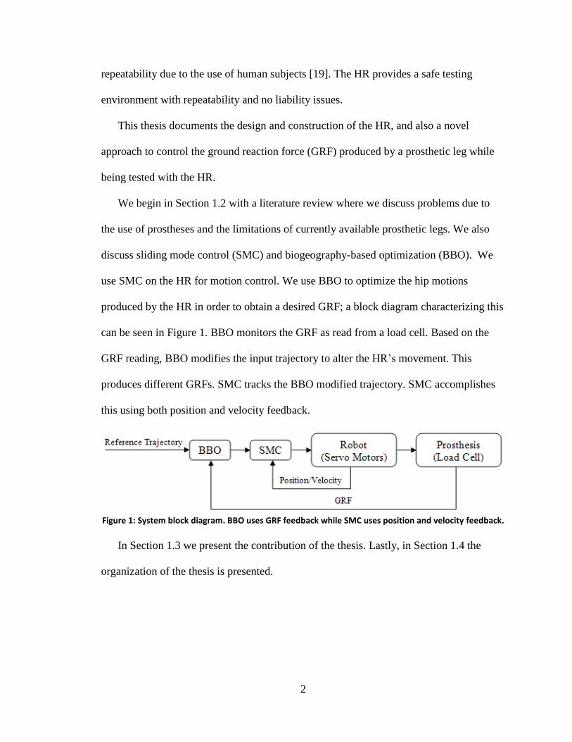
produced by the HR in order to obtain a desired GRF; a block diagram characterizing this

can be seen in Figure 1. BBO monitors the GRF as read from a load cell. Based on the

GRF reading, BBO modifies the input trajectory to alter the HR’s movement. This

produces different GRFs. SMC tracks the BBO modified trajectory. SMC accomplishes

this using both position and velocity feedback.

Figure 1: System block diagram. BBO uses GRF feedback while SMC uses position and velocity feedback.

In Section 1.3 we present the contribution of the thesis. Lastly, in Section 1.4 the

organization of the thesis is presented.

3

1.2 Literature Review

Prosthetic legs for transfemoral amputees are known to produce negative side effects

on their users [30]. Amputees alter their walking motions or gait dynamics to compensate

for the deficiencies of their prosthesis. This can cause a user to exert up to 65% more

energy than an able bodied person during normal walking [37]. This results in higher

strains and loading on the intact limb, which eventually leads to secondary physical

conditions such as osteoarthritis, osteoporosis, back pain, or joint pain [24], [30].

Secondary conditions can be due to a variety of issues, including improper alignment

of the prosthesis, improper training for the use of the prosthesis, or a poor prosthetic-

fit [30]. However, we can also attribute negative side effects to the fact that a majority of

transfemoral prosthesis users wear a passive prosthetic knee.

We define a passive prosthetic knee as one that has no source of power and is a

purely mechanical device with some form of damper. The damper typically has a spring-

loaded design and the prosthesis dissipates energy [14]. Passive knees limit a user’s gait.

They do not vary their resistance during swing phase and they do not have the ability to

self-actuate like a biological knee [13]. Because of this, prosthesis users develop gait

deviations which result in the secondary physical conditions mentioned previously [30].

An in-depth look at amputee gait with passive prostheses can be found in [36].

A more advanced prosthesis type is the variable-damper. Here a microcontroller

varies the damping or resistance of the prosthetic knee during the gait cycle to provide a

gait cycle that is closer to that of an able-bodied person. Devices that utilize a variable

damping knee are the Otto Bock C-Leg®, Össur Rheo Knee

®, and the Endolite Adaptive

Knee [25]. These designs yield promising results for users of transfemoral prostheses.

4

Variable-damping knees provide better gait stability than passive units. Unlike

passive units, they allow the user to easily change gait speeds without adjustment. Users

of variable-damping prostheses report less fatigue, easier locomotion, and more mobility

than with a passive leg [3, 22, 24]. Unfortunately, these designs still lack the ability to

deliver power at the knee, which impairs the user’s ability to have a normal gait

cycle [14].

Other prosthesis designs have elected to use an active knee. In this type of prosthesis

an electric motor or hydraulic actuator powers the knee joint. Examples include the Össur

Power KneeTM

[2] or the Bionic Leg Prosthesis with actuated knee and ankle [12, 13, 14,

15]. The goal of these prostheses is to restore power to the knee so the user can walk with

gait similar to an able bodied person. Results show that active knees do provide a gait

cycle closer to those of able-bodied biomechanics. However, these prostheses have

limited success because of their large power consumption compared to variable damping

legs and are therefore limited in their application [2].

The biggest issue facing active knees is their power sources [14]. Using lithium-ion

battery technology, the Bionic Leg Prosthesis can provide up to 9 km walking

distance [15]. This distance is expected to double in the next five years as battery

technology increases, potentially providing a prosthesis with 20 km of walking

distance [15].

The hydraulic prosthesis in development at CSU blends a variable-damping and an

active design, creating a unique semi-active knee. It consists of a hydraulic actuator, a

closed hydraulic system, and two flow valves to regulate the control of hydraulic fluid.

This design allows the prosthesis to store energy during stance-phase knee flexion. The

5

stored energy can be used to allow the user to perform movement when positive work is

necessary [2]. The knee uses a closed hydraulic system so it is always pressurized. This

means a pump is not required. The only power drawn is from the microcontroller and

opening and closing of the valves. This results in a knee that draws similar power levels

to a variable-damping knee, but includes the ability to produce positive work [38].

To develop the semi-active leg and verify its operation, an appropriate test routine

must be created. Typical tests of transfemoral prostheses are cumbersome and involve

vigorous routines with human subjects [20]. Tests require acclimation time so subjects

can become comfortable with the new prosthesis. This period of time can be up to three

months [3]. Often these tests require the use of a safety harness to prevent falling. Tests

require a gait or motion analysis lab where cameras, force plates, and other methods are

used to collect kinetic and kinematic data of the prosthetic test [2, 3, 22, 24, 25]. These

tests are not repeatable due to the often changing nature of human gait dynamics, which

can be affected by factors such as height, weight, sex, fatigue, general health, or

mood [17].

Due to the difficulties in testing prostheses, we design and construct a robot that can

test transfemoral prostheses under various walking conditions. Using a robot for testing

eliminates many of the factors present when testing with human subjects, making testing

easier. By using a robot, liability and risk of danger are virtually nonexistent. Unlike

humans, robots can operate continually without fatigue. Operation is continuous and

prostheses can be tested under repeatable conditions. Testing with robotics eliminates the

need for complex gait labs. The robot and prosthesis can be fitted with encoders, load

6

cells, and other sensors to measure quantities that are otherwise difficult to measure with

human subjects [20].

The HR project combines efforts from both the mechanical engineering (ME) and the

electrical engineering (EE) departments at CSU. We discuss construction and design of

the HR later in this thesis. To mimic the movement of a human hip, the HR uses clinical

human gait data as tracking inputs. We use SMC on the drive-stages of the HR for

feedback control.

SMC has been proven in the aerospace industry, robotics, power electronics, and

more. We choose SMC due to its popularity, ease of application, robustness, and

disturbance rejection properties [19]. In [23] SMC was used to control the flight of a

four-rotor mini flying robot. In [26] a two wheeled robot was controlled using SMC to

maintain the robot upright like an inverted pendulum. SMC will be shown in this thesis to

yield good tracking of the robot motion profiles.

Besides input tracking, we also test GRF control with the HR. When testing the robot

with able-bodied gait data, GRF of the robot did not match able-bodied GRF from the

human gait data. During these tests the drive-stages of the robot exhibited good input

tracking performance. We accept poor GRF tracking because we are using a passive knee

to simulate able-bodied walking. However, it is of interest to see if the HR could walk

with a GRF to match the able-bodied data. Doing so would require the robot to

compensate for the prosthesis, much like a human user would. To simulate human

compensation for a prosthesis and control the GRF of the HR, we modify the input

trajectories of the HR, indirectly controlling the GRF. BBO optimizes the input reference

trajectory so the desired GRF is obtained.

7

BBO is a recently developed evolutionary algorithm (EA). It has been shown to

perform better on many benchmark functions than traditional EAs, and has been applied

successfully to many real world optimization problems [6]. BBO has previously been

used to optimize the controls of CSU’s semi-active knee with initial simulation results

documented in [18, 38, 39]. For a more in-depth look at BBO, see Chapter 4.

1.3 Contribution of Thesis

This thesis documents the design, development, and construction of the HR.

Modeling techniques for drive stages of the robot and design of the controllers for those

respective systems are investigated. We evaluate human gait cycle data and show

characteristics which make it unfit to be a reference trajectory for the HR. To adjust the

data, we apply an algebraic spline interpolation method to smooth the data and solve the

problems with the raw data. The performance of the robot is evaluated based on its ability

to follow these optimized reference trajectories. Lastly we show that BBO can modify the

able-bodied gait data such that the robot walks with a desired GRF.

1.4 Organization of Thesis

Chapter 2 discusses the building of the robot. We look at the construction of the

robot, investigate the modeling of the robot, determine control parameters, and also

discuss implementation of the controllers.

Chapter 3 investigates the design of the SMC. We look at the theoretical

derivation of SMC. We present the limitations of human gait cycle data as useable

reference inputs to the HR. We then apply a smoothing optimization algorithm to make

8

the data usable as reference inputs to the HR. We lastly evaluate the performance of the

robot in following the smoothed reference trajectories.

Chapter 4 describes the method used for GRF control. We present BBO and how

it works. We then apply it to the HR to modify the input trajectories and obtain a desired

GRF. We end the chapter by examining the experimental results.

In Chapter 5 we conclude this thesis. We summarize the main ideas of the thesis

and the results from the experiments. As a final remark we look at ideas for future work.

9

CHAPTER II

CONSTRUCTION OF THE HIP ROBOT (HR)

We begin by discussing the design, construction, and modeling of the HR. In

Section 2.1, the basics of the design are presented. This discussion includes the desired

operation and motion of the HR. Section 2.2 documents the technical aspects of the HR.

Here we look at the physical components used to construct the HR. In Section 2.3 we

look at the electrical system of the robot. Section 2.4 presents the mathematical modeling

of the HR’s drive-stages. Shown also are the experiments used to determine the

parameters for those models. Lastly, in Section 2.5, we discuss the software and hardware

used to operate the robot.

2.1 Overview

Construction of the robot was a joint effort between the ME and EE departments

at CSU. The ME department designed the frame of the robot and found components that

would meet the desired specifications for the drive stages. Another account of the HR

work can be found in [20]. The research conducted as part of this thesis includes the

10

wiring and integration of the motors, drivers, and computer software into one functioning

unit.

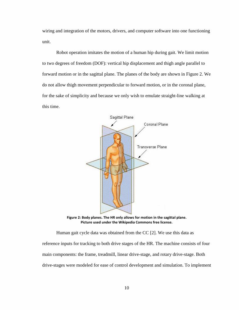
Robot operation imitates the motion of a human hip during gait. We limit motion

to two degrees of freedom (DOF): vertical hip displacement and thigh angle parallel to

forward motion or in the sagittal plane. The planes of the body are shown in Figure 2. We

do not allow thigh movement perpendicular to forward motion, or in the coronal plane,

for the sake of simplicity and because we only wish to emulate straight-line walking at

this time.

Figure 2: Body planes. The HR only allows for motion in the sagittal plane.

Picture used under the Wikipedia Commons free license.

Human gait cycle data was obtained from the CC [2]. We use this data as

reference inputs for tracking to both drive stages of the HR. The machine consists of four

main components: the frame, treadmill, linear drive-stage, and rotary drive-stage. Both

drive-stages were modeled for ease of control development and simulation. To implement

11

control of the drive stages and all other operating functions of the robot, Simulink® and

dSpace® software and hardware are used.

2.2 Electrical and Mechanical Components

The frame was designed so that it can withstand forces generated by the actuation

of the drive stages and prosthesis. Nuts, bolts, and fasteners were selected to meet those

criteria as well. The frame is constructed of welded A500 rectangular steel tubing using

bolts to attach mounting plates for drive-stages and the treadmill. All joints were verified

for static loading and fatigue using SolidWorks® software. Component life was also

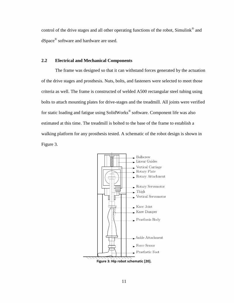
estimated at this time. The treadmill is bolted to the base of the frame to establish a

walking platform for any prosthesis tested. A schematic of the robot design is shown in

Figure 3.

Figure 3: Hip robot schematic [20].

12

The linear drive-stage consists of a brushless DC servo-motor, servo amplifier,

and ballscrew-driven linear slide. We configure the servo amplifier to run in torque mode

so the analog input voltage is theoretically proportional to the output torque of the motor.

The ballscrew mounts vertically to the robot frame to provide variation of vertical hip

displacement. The ballscrew has 12 inches of travel but on average we use only 100 mm

of travel for different motion profiles. We use the remaining distance to adjust the center

of oscillation so shorter or longer prostheses can be tested. An incremental encoder

attached to the servo motor measures both position and velocity. Absolute position of the

ballscrew is achieved using a limit switch on the top end of travel of the linear slide.

Table I shows the parameters of the drive stage.

Linear Drive-Stage

Servo Amplifier Manufacturer Mitsubishi

Model No. MR-J3-70A

Configuration Torque Mode

Servo Motor Manufacturer Mitsubishi

Model No. HF-KP73

Rated / Max Speed 3000 / 6000 RPM

Torque Rated / Max 7.2 / 8.36 Nm

Inertia Moment 1.43E-4 J-Kg-m2

Current Rated / Max 5.2 / 15.6 A

Linear Slide Manufacturer RAF Automation

Usable Travel 12 in

Lead 0.5 in / revolution Table I: Linear drive-stage parameters.

The rotary drive-stage also contains a brushless DC servo-motor and servo

amplifier. The motor drives a rotary-stage via a direct coupling and an inchworm-gear

reducer. Like the linear drive-stage, the servo amplifier is also configured for torque

mode. The entire rotary stage attaches to the linear slide’s carriage, so the entire rotary

drive-stage moves vertically when varying vertical hip displacement. When operating we

establish absolute position of the rotary stage with a limit switch. Angular position and

13

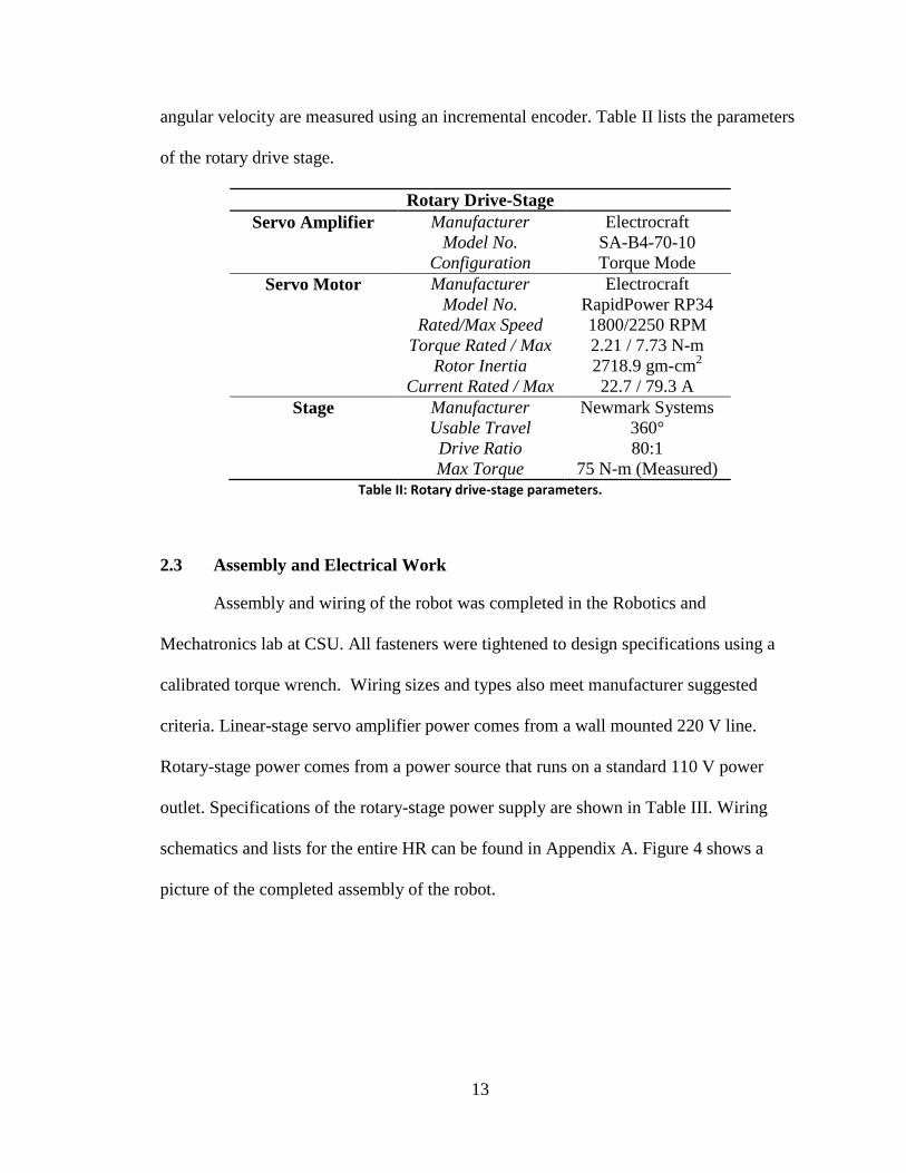
angular velocity are measured using an incremental encoder. Table II lists the parameters

of the rotary drive stage.

Rotary Drive-Stage

Servo Amplifier Manufacturer Electrocraft

Model No. SA-B4-70-10

Configuration Torque Mode

Servo Motor Manufacturer Electrocraft

Model No. RapidPower RP34

Rated/Max Speed 1800/2250 RPM

Torque Rated / Max 2.21 / 7.73 N-m

Rotor Inertia 2718.9 gm-cm2

Current Rated / Max 22.7 / 79.3 A

Stage Manufacturer Newmark Systems

Usable Travel 360°

Drive Ratio

Max Torque

80:1

75 N-m (Measured) Table II: Rotary drive-stage parameters.

2.3 Assembly and Electrical Work

Assembly and wiring of the robot was completed in the Robotics and

Mechatronics lab at CSU. All fasteners were tightened to design specifications using a

calibrated torque wrench. Wiring sizes and types also meet manufacturer suggested

criteria. Linear-stage servo amplifier power comes from a wall mounted 220 V line.

Rotary-stage power comes from a power source that runs on a standard 110 V power

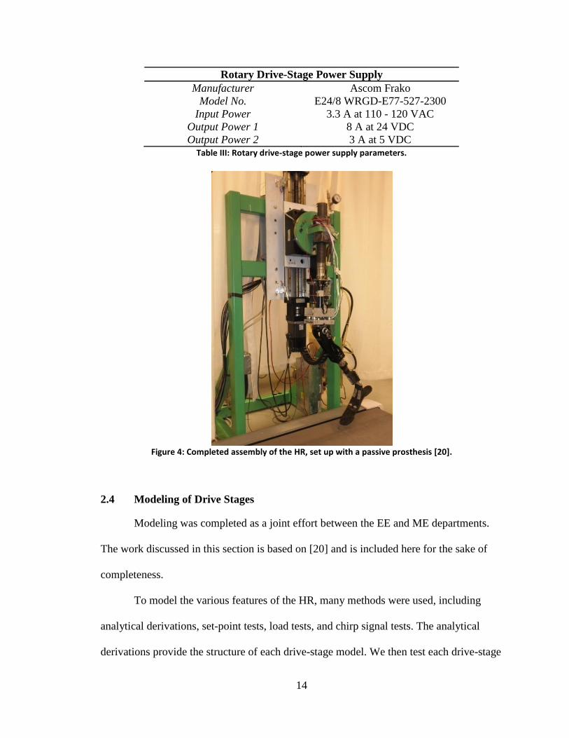
outlet. Specifications of the rotary-stage power supply are shown in Table III. Wiring

schematics and lists for the entire HR can be found in Appendix A. Figure 4 shows a

picture of the completed assembly of the robot.

14

Rotary Drive-Stage Power Supply

Manufacturer Ascom Frako

Model No. E24/8 WRGD-E77-527-2300

Input Power 3.3 A at 110 - 120 VAC

Output Power 1 8 A at 24 VDC

Output Power 2 3 A at 5 VDC Table III: Rotary drive-stage power supply parameters.

Figure 4: Completed assembly of the HR, set up with a passive prosthesis [20].

2.4 Modeling of Drive Stages

Modeling was completed as a joint effort between the EE and ME departments.

The work discussed in this section is based on [20] and is included here for the sake of

completeness.

To model the various features of the HR, many methods were used, including

analytical derivations, set-point tests, load tests, and chirp signal tests. The analytical

derivations provide the structure of each drive-stage model. We then test each drive-stage

15

to find values for variables within those model structures. Since both stages are

configured to run in torque mode we can model them as current driven DC machines with

inertias:

(2.1)

where τ represents torque of the motor, J the total inertia of the stage, angular

acceleration, the input current, and k the torque constant of the motor.

2.4.1 Analytical Derivation

For the vertical stage we ignore viscous damping and concern ourselves with

friction of the carriage on the guides. This provides the following ballscrew torque

balance equation:

(2.2)

where represents motor torque and represents torque due to the reaction of the

carriage on the screw. We also know that a ballscrew with lead and efficiency has

thrust force F:

(2.3)

We define motor torque as follows:

(2.4)

where relates input voltage of the servo amplifier to output torque, and is the input

voltage. Combining Equations 2.2, 2.3, and 2.4 gives the total thrust force that the motor

delivers to the carriage:

(2.5)

16

The rotary-stage can be modeled more simply using the basic model for a DC

current driven machine. We consider viscous damping due to the drivetrain and account

for the internal gear ratio (80:1) of the drive-stage. We take the Laplace transform of

Equation 2.1 and include the viscous damping coefficient :

(2.6)

where represents the input voltage, a constant which relates input voltage of the

servo amplifier to output torque, the inertia of the rotary stage actuator gear, the gear

ratio, and the inertia of the worm gear and motor armature.

2.4.2 Parameter Estimation

Each drive stage was operated though various tests to experimentally determine

the unknown variables in the modeling equations. For the linear drive-stage, a series of

set point tests were performed to determine . In these tests the slide’s carriage was

placed against a load cell to measure force, input voltages were then applied, and the

resultant forces were recorded. We used linear regression to determine the value for .

To determine , as given in Equation 2.3, the carriage was statically pressed

against a load cell. Thrust and torque were measured using a torque cell. Those values

were used in a linear regression equation to determine a value for . Using back

calculation, a value for efficiency was also found. Using the same torque cell, we found

braking torque of the carriage due to friction on the slides. The final values for the model

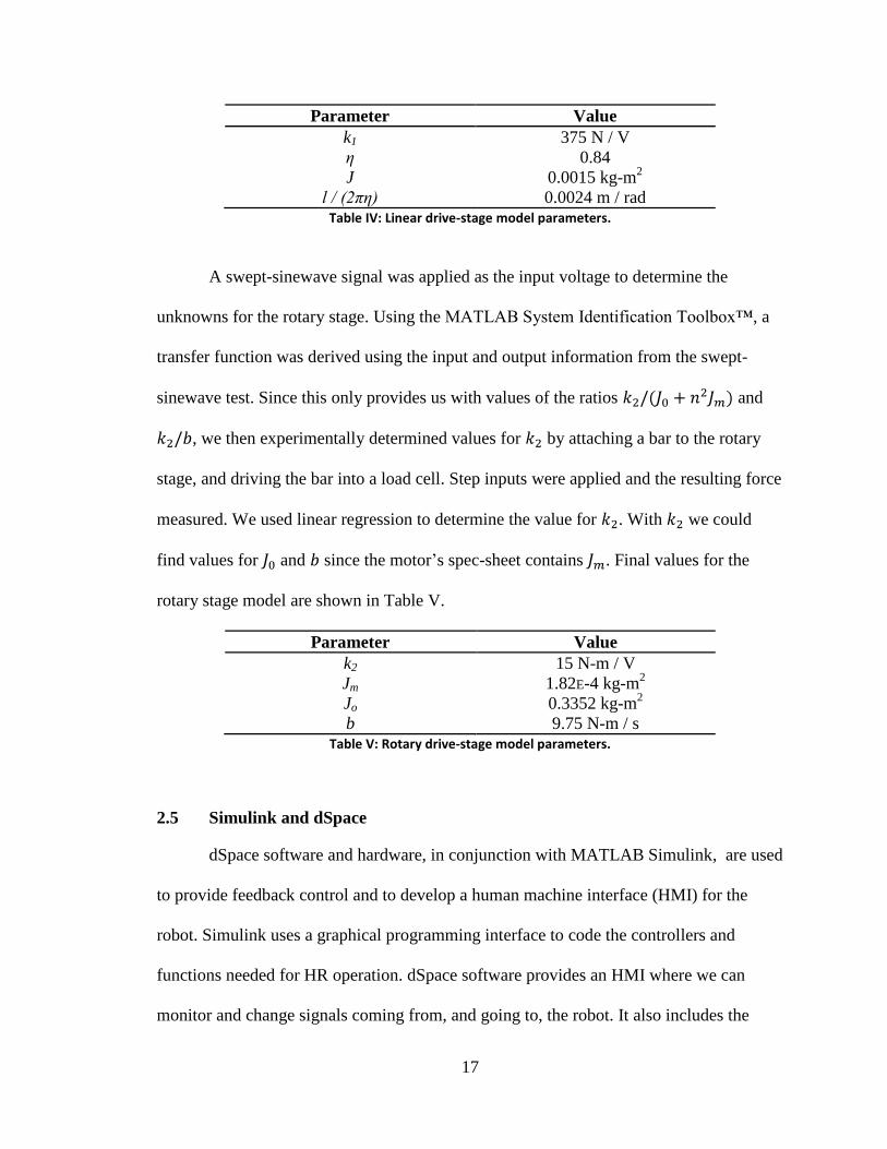
are shown in Table IV.

17

Parameter Value

k1 375 N / V

η 0.84

J 0.0015 kg-m2

l / (2πη) 0.0024 m / rad Table IV: Linear drive-stage model parameters.

A swept-sinewave signal was applied as the input voltage to determine the

unknowns for the rotary stage. Using the MATLAB System Identification Toolbox™, a

transfer function was derived using the input and output information from the swept-

sinewave test. Since this only provides us with values of the ratios and

, we then experimentally determined values for by attaching a bar to the rotary

stage, and driving the bar into a load cell. Step inputs were applied and the resulting force

measured. We used linear regression to determine the value for . With we could

find values for and since the motor’s spec-sheet contains . Final values for the

rotary stage model are shown in Table V.

Parameter Value

k2

Jm

Jo

15 N-m / V

1.82E-4 kg-m2

0.3352 kg-m2

b 9.75 N-m / s Table V: Rotary drive-stage model parameters.

2.5 Simulink and dSpace

dSpace software and hardware, in conjunction with MATLAB Simulink, are used

to provide feedback control and to develop a human machine interface (HMI) for the

robot. Simulink uses a graphical programming interface to code the controllers and

functions needed for HR operation. dSpace software provides an HMI where we can

monitor and change signals coming from, and going to, the robot. It also includes the

18

hardware necessary to do so, including an internal computer processor and external

connection board.

In the Simulink environment functions are displayed as blocks and the lines

connecting the blocks represent the signal paths. dSpace software provides blocks within

the Simulink environment that allow us to read various signals from the robot, and also to

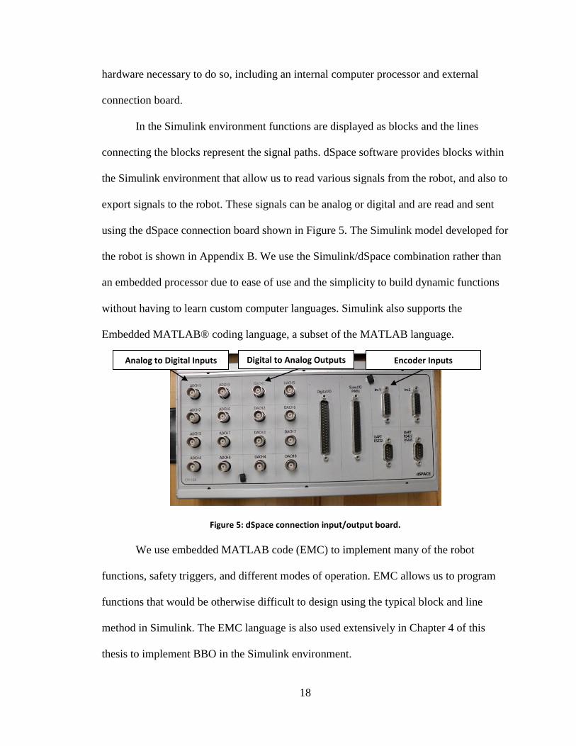
export signals to the robot. These signals can be analog or digital and are read and sent

using the dSpace connection board shown in Figure 5. The Simulink model developed for

the robot is shown in Appendix B. We use the Simulink/dSpace combination rather than

an embedded processor due to ease of use and the simplicity to build dynamic functions

without having to learn custom computer languages. Simulink also supports the

Embedded MATLAB® coding language, a subset of the MATLAB language.

Figure 5: dSpace connection input/output board.

We use embedded MATLAB code (EMC) to implement many of the robot

functions, safety triggers, and different modes of operation. EMC allows us to program

functions that would be otherwise difficult to design using the typical block and line

method in Simulink. The EMC language is also used extensively in Chapter 4 of this

thesis to implement BBO in the Simulink environment.

Digital to Analog Outputs Analog to Digital Inputs Encoder Inputs

19

We use dSpace software to create the HMI for the robot. The software actively

communicates with the Simulink model. This allows us to display and adjust values

within the Simulink model in real time. Some of the basic dSpace operators that we use,

such as the slider, input box, plotter, display, and selector button, are discussed in

Appendix C. The complete HR dSpace HMI used for this thesis can also be found in

Appendix C.

2.6 Ground Reaction Force (GRF) Measurement

When testing the HR, GRF is measured with a load cell attached to the prosthetic

leg. Using a custom bracket, the load cell mounts between the prosthetic knee and foot.

This is shown in Figures 3 and 10. Positioning the load cell at that location does not read

GRF directly but measures force along the lower shank of the prosthesis. For GRF

optimization, the measured force along the lower shank needs to be compared to the force

from the reference gait data. The force along the lower shank is not provided in the gait

cycle data; however, the three-dimensional decomposition of GRF is provided.

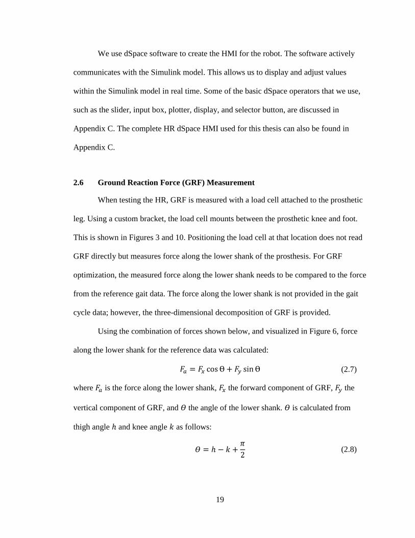
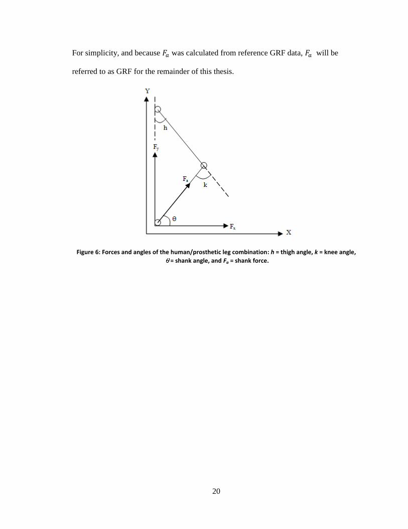
Using the combination of forces shown below, and visualized in Figure 6, force

along the lower shank for the reference data was calculated:

(2.7)

where is the force along the lower shank, the forward component of GRF, the

vertical component of GRF, and the angle of the lower shank. is calculated from

thigh angle and knee angle as follows:

(2.8)

20

For simplicity, and because was calculated from reference GRF data, will be

referred to as GRF for the remainder of this thesis.

Figure 6: Forces and angles of the human/prosthetic leg combination: h = thigh angle, k = knee angle,

= shank angle, and Fa = shank force.

21

CHAPTER III

SLIDING MODE CONTROL (SMC)

In this chapter we present the design, implementation, and performance of the

control system used for HR operation. We begin in Section 3.1 with a general overview

of SMC. We discuss why we use SMC, and some of its drawbacks. Section 3.2 presents

the mathematical derivation of a version of SMC applicable to the actuator models.

Section 3.3 investigates the problems associated with using human gait data as tracking

references to the HR. We address those problems by adjusting the gait cycle data using an

optimization algorithm. In Section 3.4 we implement the controller on the HR. We

present the use of Simulink, dSpace, and real time tuning methods for the controller.

Section 3.5 presents the operation of the robot, where the HR is fitted with a prosthesis

and tested. Lastly we examine the tracking of the robot compared to the reference motion

profiles and analyze the performance of both controller and HR.

22

3.1 Overview

For control purposes we treat the robot as two independent closed loop single

input single output (SISO) systems. The mechanical configuration of the robot allows us

to do so by ignoring the forces generated between drive-stages. We assume the rotary

drive-stages high gear ratio makes it non-back-drivable. For the vertical stage we assume

that swinging the leg with the rotary stage will produce only small inertial changes that

affect the linear stage [20].

We choose sliding mode control (SMC) due to its straightforward application and

robustness properties [19]. SMC was developed in the late 1950’s in the former Soviet

Union by professors V. I. Utkin and S. V. Emelyanov [41]. It is a nonlinear control

technique in which invariance properties guarantee disturbance rejection and robustness

under some conditions.

Unlike a PID or similar controller, SMC does not require real-time integration or

differentiation, which makes computer processing less of a burden. SMC is a switching

algorithm and therefore susceptible to chattering [19]. It requires three inputs: the

reference signal to be tracked, the reference signal’s first derivative, and the reference

signal’s second derivative. When computing these derivatives, SMC requires smoothness

of the signal and its derivatives. In most cases these derivatives are calculated off-line in

order to avoid the need for real time differentiation of the input trajectory.

23

3.2 Derivation of Sliding Mode Control

In SMC we define a sliding manifold towards which we drive the system. For our

purposes we follow the derivation of a basic SISO SMC which can be found in [19]. For

a SISO system with desired response and output the error is defined as:

(3.1)

We then define as the sliding function:

(3.2)

where represents a constant tuning parameter of the controller. Introducing

requires reference data and feedback . When the system is driven to the sliding

function, and consequently . To accomplish this we constrain the

derivative of to the signum function times a constant tuning parameter :

(3.3)

This guarantees that as time increases, goes to zero in some finite amount of time.

When the sliding function is reached. Taking the derivative of Equation 3.2 gives:

(3.4)

Substituting for , , and , we get:

(3.5)

This will be used later to derive our control signal . Our drive-stages can be modeled as

DC current-driven machines with damping:

(3.6)

where is the control signal, the combination servo amplifier gain and motor torque,

the inertia in the system, and the viscous damping. Simplifying Equation 3.6, taking

derivatives where necessary, and accounting for unknown torque disturbance gives:

24

(3.7)

The torque disturbance is ignored when deriving the control law. As shown in [20], its

effects can be entirely rejected by choosing a sufficiently large , provided the

disturbance is bounded by a known constant. Solving (3.7) for and substituting into

Equation 3.5 yields:

(3.8)

Solving for we get the resultant control signal:

(3.9)

Note in Equation 3.4 that . Therefore we need to calculate and ,

which means our controller also requires output and inputs and . From the motor

encoders we have feedback for position and velocity, or and . To achieve SMC we

need reference data and . Because of this, the input signal must be twice

differentiable. Due to differentiability, it is also continuous. Since is the reference

trajectory, these derivatives can be calculated off-line or before they are used as inputs to

the system to avoid the need for real-time differentiation.

3.3 Hip Robot Reference Input Trajectory Smoothing

Clinical human gait data for thigh angle and vertical hip displacement are used as

inputs to the robot to emulate human hip motion. The CC provided the gait cycle data,

which has limitations. Because of measuring methods, the data is only one stride or

period in length. If the robot needs to operate for more than one stride, the data needs to

be repeated cyclically. However, the data does not end at a point close to the start point.

Because of this, when it is repeated, noise appears in the first derivative, and

25

consequently in the second derivative as well. Since SMC requires smoothness of the

signal and its first two derivatives, we must adjust the input data to avoid those issues. In

order to do this we smooth the data using an optimization algorithm.

3.3.1 Reference Input Trajectory Optimization

Optimization provides a straightforward way to smooth the reference data. The

reference input trajectories must satisfy two criteria. First, they must be defined within

the three-dimensional space that the robot can move. Second, position, velocity, and

acceleration must be continuous [35]. Generally we optimize the trajectory in between

data points in order to minimize negative effects on the robot [9]. For our purpose, we

have the predetermined clinical data that consists of many points that the robot must

follow.

We can represent the gait cycle data using either a single polynomial or multiple

polynomials splined together between concurrent data points. Using a single polynomial

results in an extremely high order trajectory [34]. When constraining derivatives for

smoothness the order is even higher [35]. Therefore we spline together multiple low order

polynomials between adjacent data points to reduce the order and computational load of

the trajectory [34]. We perform optimization using algebraic spline interpolation, and

minimize the sum of squared error between the original data and the spline at the data

points. Algebraic spline interpolation is used due to its popularity, simplicity, and ease of

use [9]. We constrain the data in order to maintain the integrity of the original signal,

resulting in a smoothed signal that closely resembles the original.

Algebraic spline interpolation represents the signal between each pair of data

points using a polynomial. For the hip robot we require continuity of the input signal,

26

first derivative, and second derivative. For that reason we use a third order polynomial

between each pair of data points [4]. Typically a higher order polynomial will be more

likely to contain unnecessary oscillations [9]. We define our polynomial between two

adjacent data point as follows:

(3.10)

where the terms represent the polynomial coefficients. The interpolated signal is

therefore:

(3.11)

where , and , where n is the total number of data points in the

clinically provided human gait data. This yields a family of polynomial functions,

each with four coefficients to represent the smoothed signal.

The algebraic spline method allows us to impose multiple constraints to adapt the

optimization objective to our specific needs. For our purpose we want the data trajectory

to be continuous and end at the same point as it starts, allowing us to repeat the gait cycle

without discontinuities. We impose constraints for continuity:

(3.12)

for and constraints for the start and end points:

(3.13)

where is the time at the end of the gait cycle.

27

Using the constraints from (3.12) and (3.13), we use MATLAB function

quadprog to implement the algebraic spline optimization. We minimize the sum of

squared error defined as:

(3.14)

where is the smoothed spline signal at time , and is the original data at index .

We optimize this subject to the constraint equations in (3.12) and (3.13). Since

we have a third order representation of the signal, with data points, we optimize to find

unknowns.

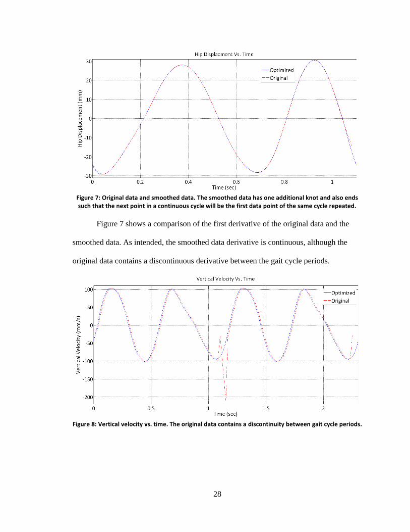
3.3.2 Optimization Results

Results are shown in Figures 7 and 8. Figure 7 compares the original data and the

smoothed data. We add one additional knot to the spline to aid the smoothing algorithm.

As constrained, the next point after the end point of the smoothed data will be the start

point of the next period of the smoothed data. This guarantees continuity between

repetitions of the gait cycle data. Figure 6 shows the third order algebraic spline,

maintaining the integrity of the original signal. Note that the original data is not periodic,

but the spline is periodic.

28

Figure 7: Original data and smoothed data. The smoothed data has one additional knot and also ends such that the next point in a continuous cycle will be the first data point of the same cycle repeated.

Figure 7 shows a comparison of the first derivative of the original data and the

smoothed data. As intended, the smoothed data derivative is continuous, although the

original data contains a discontinuous derivative between the gait cycle periods.

Figure 8: Vertical velocity vs. time. The original data contains a discontinuity between gait cycle periods.

29

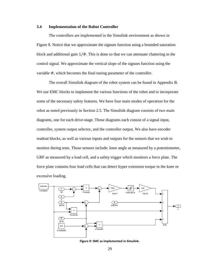
3.4 Implementation of the Robot Controller

The controllers are implemented in the Simulink environment as shown in

Figure 8. Notice that we approximate the signum function using a bounded saturation

block and additional gain . This is done so that we can attenuate chattering in the

control signal. We approximate the vertical slope of the signum function using the

variable , which becomes the final tuning parameter of the controller.

The overall Simulink diagram of the robot system can be found in Appendix B.

We use EMC blocks to implement the various functions of the robot and to incorporate

some of the necessary safety features. We have four main modes of operation for the

robot as noted previously in Section 2.5. The Simulink diagram consists of two main

diagrams, one for each drive-stage. Those diagrams each consist of a signal input,

controller, system output selector, and the controller output. We also have encoder

readout blocks, as well as various inputs and outputs for the sensors that we wish to

monitor during tests. Those sensors include: knee angle as measured by a potentiometer,

GRF as measured by a load cell, and a safety trigger which monitors a force plate. The

force plate contains four load cells that can detect hyper extension torque in the knee or

excessive loading.

Figure 9: SMC as implemented in Simulink.

30

There are multiple safety triggers to prevent damage to the robot and ensure

operator safety. There are limit switches to indicate if the robot has traveled outside of its

safe operating range. We have a user controlled emergency stop button which

immediately deactivates all robot functions. Velocity and acceleration limits are

programmed into the servo amplifiers. Saturation blocks in the Simulink diagram prevent

any analog signals from going outside of their safe operating ranges. Finally, a rate

transition block prevents the vertical displacement reference from changing too quickly.

The robot operator monitors GRF and deactivates the robot if unsafe readings are

measured.

Tuning of the controller was performed in real time with dSpace. Since dSpace

allows the manipulation of variables in real time, we configured dSpace sliders for each

tuning parameter of the SMCs. The stages were run and the sliders adjusted until proper

tracking was obtained. Adjusting allowed us to control the approximation of the

signum function and attenuated chattering of the system. Adjusting varied the

switching gain of the system. Generally the higher is, the less susceptible to

disturbances the system became, but increases in also increased chattering. Modifying

adjusted the convergence speed of the error to the sliding manifold. The values for and

are extremely robust and have a wide range in which the robot operation is acceptable.

The system is most sensitive to the adjustment of since this is the assumed slope we

use for the signum function and has an immediate effect on chatter. The final control

gains for both linear and rotary drive-stages are shown in Table VI.

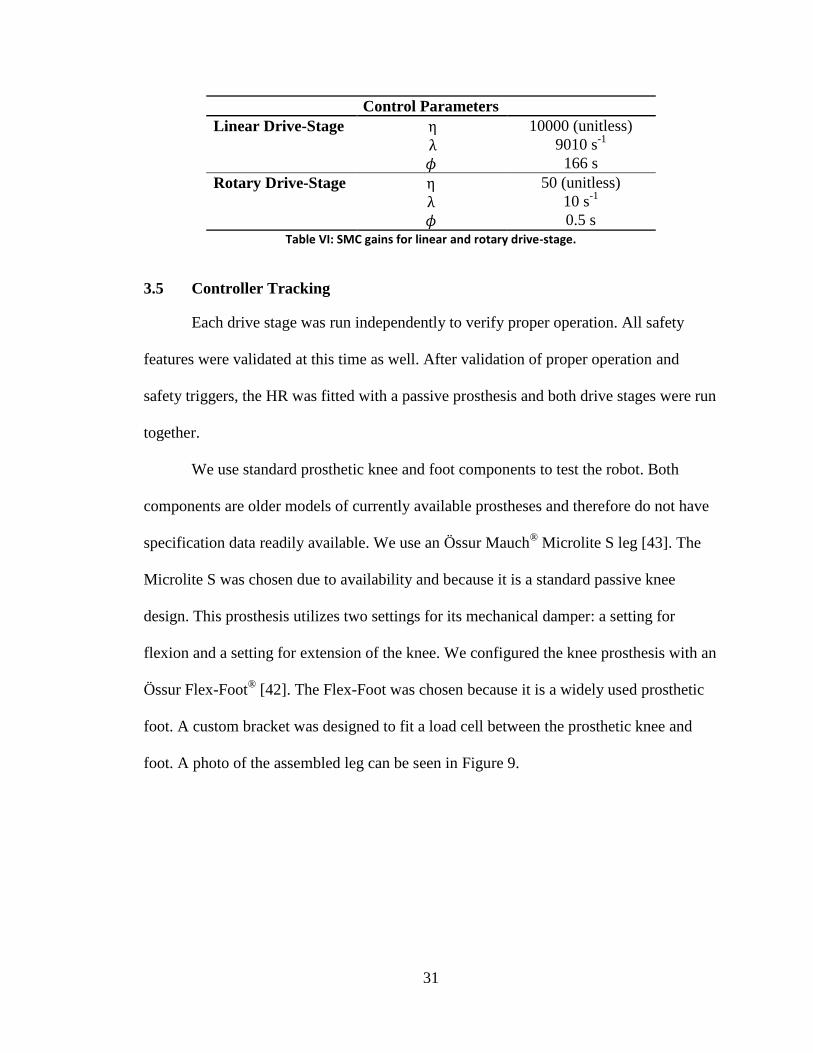
31

Control Parameters

Linear Drive-Stage 10000 (unitless)

9010 s-1

166 s

Rotary Drive-Stage 50 (unitless)

10 s-1

0.5 s

Table VI: SMC gains for linear and rotary drive-stage.

3.5 Controller Tracking

Each drive stage was run independently to verify proper operation. All safety

features were validated at this time as well. After validation of proper operation and

safety triggers, the HR was fitted with a passive prosthesis and both drive stages were run

together.

We use standard prosthetic knee and foot components to test the robot. Both

components are older models of currently available prostheses and therefore do not have

specification data readily available. We use an Össur Mauch® Microlite S leg [43]. The

Microlite S was chosen due to availability and because it is a standard passive knee

design. This prosthesis utilizes two settings for its mechanical damper: a setting for

flexion and a setting for extension of the knee. We configured the knee prosthesis with an

Össur Flex-Foot® [42]. The Flex-Foot was chosen because it is a widely used prosthetic

foot. A custom bracket was designed to fit a load cell between the prosthetic knee and

foot. A photo of the assembled leg can be seen in Figure 9.

32

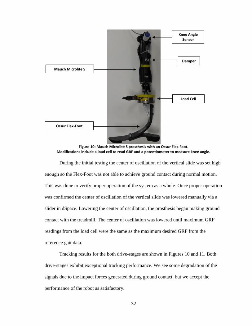
Figure 10: Mauch Microlite S prosthesis with an Össur Flex Foot.

Modifications include a load cell to read GRF and a potentiometer to measure knee angle.

During the initial testing the center of oscillation of the vertical slide was set high

enough so the Flex-Foot was not able to achieve ground contact during normal motion.

This was done to verify proper operation of the system as a whole. Once proper operation

was confirmed the center of oscillation of the vertical slide was lowered manually via a

slider in dSpace. Lowering the center of oscillation, the prosthesis began making ground

contact with the treadmill. The center of oscillation was lowered until maximum GRF

readings from the load cell were the same as the maximum desired GRF from the

reference gait data.

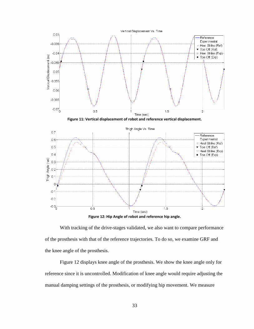
Tracking results for the both drive-stages are shown in Figures 10 and 11. Both

drive-stages exhibit exceptional tracking performance. We see some degradation of the

signals due to the impact forces generated during ground contact, but we accept the

performance of the robot as satisfactory.

Knee Angle Sensor

Össur Flex-Foot

Load Cell

Damper

Mauch Microlite S

33

Figure 11: Vertical displacement of robot and reference vertical displacement.

Figure 12: Hip Angle of robot and reference hip angle.

With tracking of the drive-stages validated, we also want to compare performance

of the prosthesis with that of the reference trajectories. To do so, we examine GRF and

the knee angle of the prosthesis.

Figure 12 displays knee angle of the prosthesis. We show the knee angle only for

reference since it is uncontrolled. Modification of knee angle would require adjusting the

manual damping settings of the prosthesis, or modifying hip movement. We measure

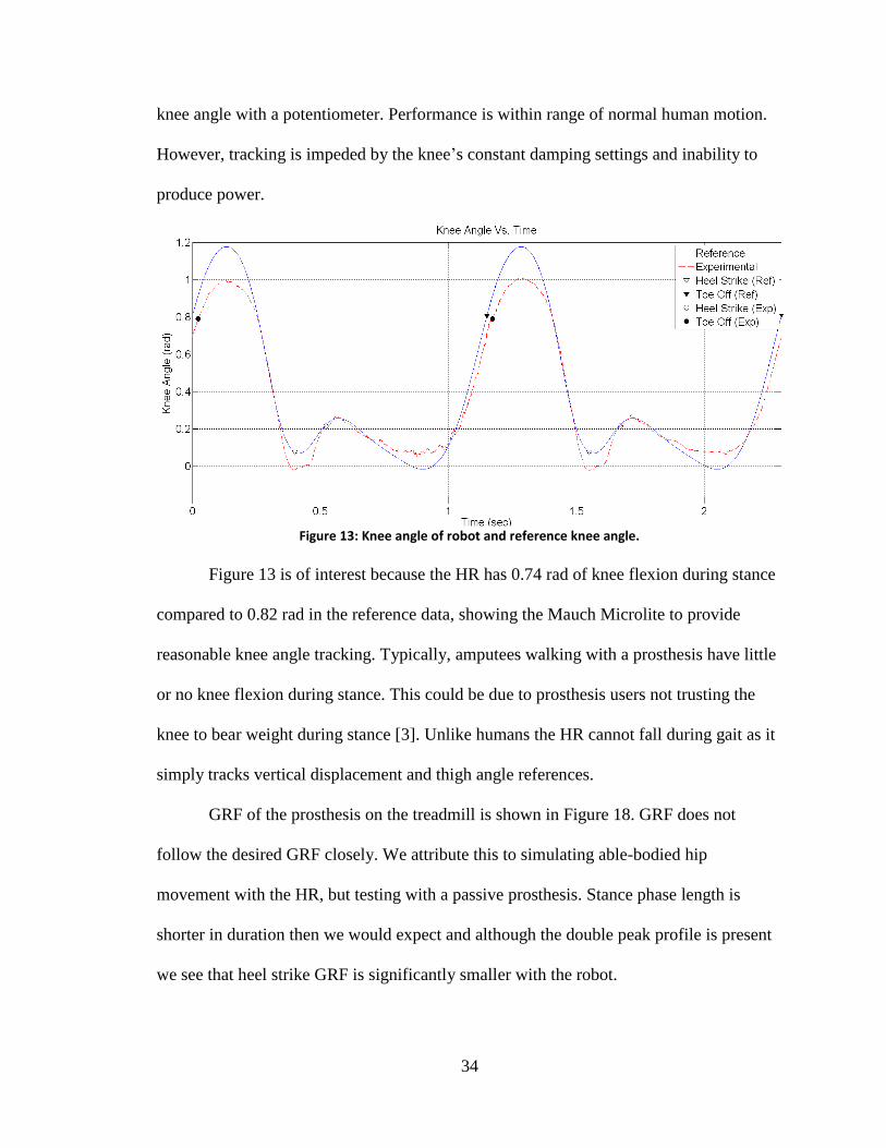
34

knee angle with a potentiometer. Performance is within range of normal human motion.

However, tracking is impeded by the knee’s constant damping settings and inability to

produce power.

Figure 13: Knee angle of robot and reference knee angle.

Figure 13 is of interest because the HR has 0.74 rad of knee flexion during stance

compared to 0.82 rad in the reference data, showing the Mauch Microlite to provide

reasonable knee angle tracking. Typically, amputees walking with a prosthesis have little

or no knee flexion during stance. This could be due to prosthesis users not trusting the

knee to bear weight during stance [3]. Unlike humans the HR cannot fall during gait as it

simply tracks vertical displacement and thigh angle references.

GRF of the prosthesis on the treadmill is shown in Figure 18. GRF does not

follow the desired GRF closely. We attribute this to simulating able-bodied hip

movement with the HR, but testing with a passive prosthesis. Stance phase length is

shorter in duration then we would expect and although the double peak profile is present

we see that heel strike GRF is significantly smaller with the robot.

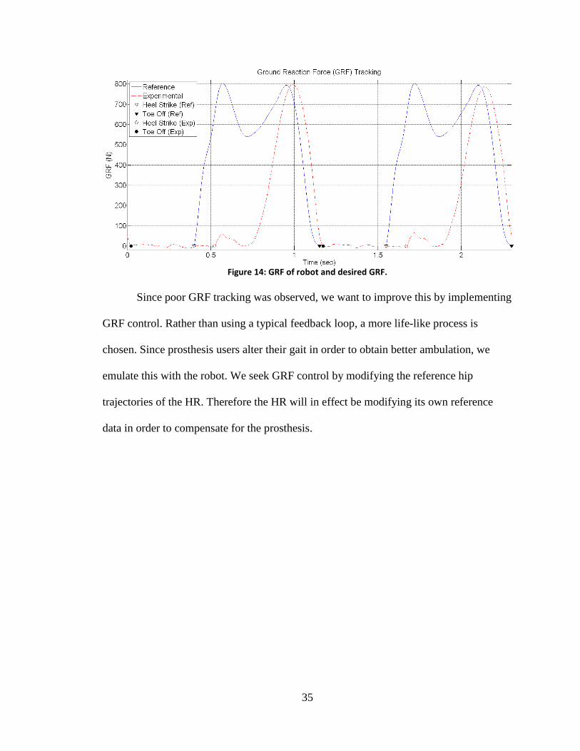
35

Figure 14: GRF of robot and desired GRF.

Since poor GRF tracking was observed, we want to improve this by implementing

GRF control. Rather than using a typical feedback loop, a more life-like process is

chosen. Since prosthesis users alter their gait in order to obtain better ambulation, we

emulate this with the robot. We seek GRF control by modifying the reference hip

trajectories of the HR. Therefore the HR will in effect be modifying its own reference

data in order to compensate for the prosthesis.

36

CHAPTER IV

GROUND REACTION FORCE CONTROL

Throughout this Chapter we discuss the implementation of BBO to control GRF

of the HR. We start in Section 4.1 with a general overview of how we apply BBO to the

HR in order to control GRF. Section 4.2 provides a description BBO. In Section 4.3 we

discuss the application of BBO to both the HR simulation and HR hardware. Section 4.4

presents the HR simulation. Here we explain the goals of the simulation and the

simulation results. Finally in Section 5.5 we apply BBO to the HR hardware to control

GRF. We apply BBO in two distinct optimization phases and discuss our final results.

4.1 Overview

The HR tracks the reference motion profiles as shown in the previous chapter.

However, those results show the deficiencies of a passive prosthesis. GRF and knee angle

do not follow the reference profiles. We do not address knee angle tracking since the

passive prosthesis knee is uncontrollable. However, we can control GRF of the

prosthesis. Rather than controlling GRF with a feedback loop, we choose to indirectly

37

control the GRF by adjusting the reference trajectories during the stance phase of gait.

We use BBO to adjust the reference data for the HR. This will make the robot

compensate for the passive prosthesis, like an actual amputee using the same prosthesis

would.

4.2 Biogeography-Based Optimization (BBO)

BBO is an EA which uses the geographical distribution of biological species as its

foundation. The study of biogeography examines the speciation, migration, mutation, and

extinction of organisms in nature. BBO represents and simulates this process [6]. It has

been applied to numerous problems, including aircraft engine sensor selection [6], control

of wall following robots [1], electrocardiogram parameter identification [5], and

prosthetic knee control [39].

In nature a habitat contains species or individuals. These individuals can migrate

between habitats based on how well a habitat is suited for supporting life. We measure

this as the habitat suitability index (HSI). The factors that influence HSI are suitability

index variables (SIVs). An SIV can be things such as rainfall, topography, temperature,

or abundance of vegetation [6]. In essence an HSI can be thought of as the dependent

variable of a habitat and an SIV the independent variable [5].

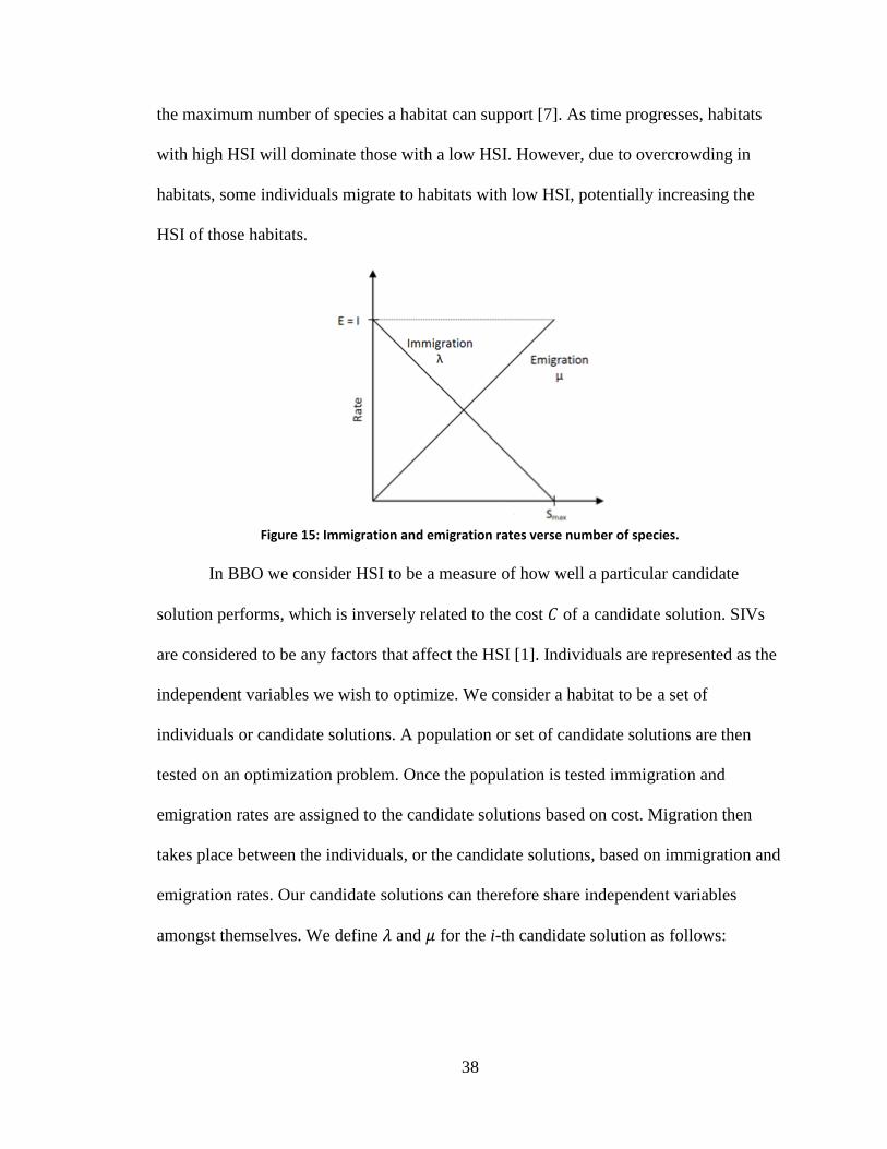
A high HSI means the habitat is highly suitable for life and therefore has a high

emigration rate and low immigration rate. Conversely, a habitat with low HSI has a high

immigration rate and low emigration rate. An example of this is shown in Figure 19,

where is the immigration rate, the emigration rate, and the number of species,

which is directly correlated with HSI. Maximum immigration to a habitat occurs when

there are no species in that habitat and maximum emigration occurs when ,

38

the maximum number of species a habitat can support [7]. As time progresses, habitats

with high HSI will dominate those with a low HSI. However, due to overcrowding in

habitats, some individuals migrate to habitats with low HSI, potentially increasing the

HSI of those habitats.

Figure 15: Immigration and emigration rates verse number of species.

In BBO we consider HSI to be a measure of how well a particular candidate

solution performs, which is inversely related to the cost of a candidate solution. SIVs

are considered to be any factors that affect the HSI [1]. Individuals are represented as the

independent variables we wish to optimize. We consider a habitat to be a set of

individuals or candidate solutions. A population or set of candidate solutions are then

tested on an optimization problem. Once the population is tested immigration and

emigration rates are assigned to the candidate solutions based on cost. Migration then

takes place between the individuals, or the candidate solutions, based on immigration and

emigration rates. Our candidate solutions can therefore share independent variables

amongst themselves. We define and for the i-th candidate solution as follows:

39

(4.1)

where represents the total number of candidate solutions in a population, , n is

the total number of candidate solutions in the BBO population, and is the fitness rank

of candidate solution , where the best candidate solution has a rank of 1 and the worst

has a rank of .

Similar to many EAs, BBO also implements elitism and mutation. Elitism allows

us to maintain the best candidate solution(s) from one generation to the next, assuring us

that the best candidate solutions are never lost [39]. Mutation increases diversity and adds

new information into the population [6].

4.3 Application of BBO to GRF Optimization

We apply BBO in both simulation and hardware. In both applications BBO

creates a continuous delta displacement signal which is added to the vertical displacement

reference. When we apply BBO to the robot we also optimize the zero-offsets or bias of

the reference data, but this is not necessary in simulation. This is discussed later in

Section 4.4. Here we discuss concepts that can be applied to both the simulation and

hardware applications of BBO.

We choose to add a delta displacement signal to the vertical displacement

reference trajectory. This is done so the original signal is not lost, which allows us to use

the original trajectory as an experimental control and initial condition. We create the delta

displacement signal using a Fourier series representation. BBO optimizes the Fourier

40

coefficients based on error between reference GRF and experimental GRF. To ease

computation we parameterize each candidate delta displacement signal as a Fourier

cosine series rather than a full Fourier series:

(4.2)

where is half of the control duration. Control duration is only during stance phase of

the gait cycle. is the number of Fourier coefficients. There are thus independent

variables to be optimized in the problem. is a tradeoff between search resolution and

problem size. is half of the signal duration so we can use the cosine series rather than

the full Fourier series, which reduces the dimension of the problem by almost 50% [16].

is an even function on the time interval , but we only apply the control

signal between time 0 and T.

To change the candidate solution into a delta-displacement signal, u(t) is

calculated from Equation (4.2) in real time. Since the HR uses SMC, we need an input

reference signal and its first two derivatives. To calculate the first two derivatives of the

delta-displacement signal, real time derivatives are calculated using a low pass filter

approximation which is shown in Equation (4.3).

(4.3)

where . Analytical derivatives could be used, however the reference data is

smooth enough that the approximation works satisfactorily.

The first candidate solution tested for each BBO simulation is the Fourier

coefficient set containing all zeros. This candidate solution, when added to the reference

data, produces no change in the reference data. This guarantees that we will always begin

41

the optimization process with the original reference data as the initial condition of the

BBO simulation.

4.4 Hip Robot (HR) Simulation

Before we use BBO on the HR hardware, we verify that BBO can modify the

vertical displacement motion profile using a Simulink simulation developed in [20],

which simulates HR operation. Doing so allows us to develop an appropriate BBO

process without risking unexpected or potentially harmful behavior to the HR. The

simulation utilizes a Hybrid Swing-Stance Model [20] for the HR and can predict

tracking performance of both drive-stages, knee angle of the prosthesis, and GRF of the

HR. The simulation utilizes the same model parameters for both drive-stages and the

SMC as derived in this thesis and in [20]. We do not pursue perfect GRF tracking with

the simulation due to the differences between the simulation and the robot hardware. The

simulation does not have a model for a prosthetic foot. It simulates the HR’s GRF by

means of a single point of ground contact, or peg leg, where as the robot tests prostheses

with a prosthetic foot. Therefore the simulation does not reproduce heel strike and toe off

conditions appropriately, and GRF from the simulation does not adequately simulate

GRF of the HR. We therefore use the simulation only to develop the BBO procedure for

the HR in order to avoid potentially hazardous situations. Simulation results only confirm

that the concept will be feasible on the HR hardware.

4.4.1 Simulation Characteristics

Simulations were run on a 24-core processor PC. Using MATLAB’s parallel

processing toolbox, simulations can run across a maximum of twelve cores. This means

42

that MATLAB can support 12 parallel processes or simulations. However, due to the

high computational demand of the HR simulation, we were only able to use eight parallel

simulations running across twelve cores. Using any more than 8 parallel simulations

would cause the optimization to crash due to lack of memory.

The simulation was updated to include a series of custom-made rate-limit and

saturation blocks in Simulink. These simulated the safety limits built into the robot. If any

of these limits were reached, the cost for the BBO candidate solution being tested was

assigned a high value as reaching these limits is undesirable.

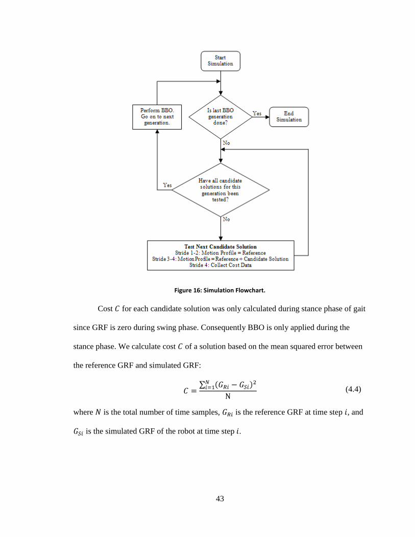
The test sequence for the simulation is shown in Figure 16. For each candidate

solution, the HR simulation was run for a series of four strides or complete gait cycles.

The first two strides were used to provide the same initial conditions for each candidate

solution. During these steps the simulation would be run using the unaltered reference

vertical displacement. The third and fourth steps then add the delta displacement signal to

the reference data. We use two steps because it was found that the HR in both simulation

and in experimental hardware needed at least one step before it reached consistent

operating conditions. Cost was calculated based on the GRF of the fourth gait cycle.

43

Figure 16: Simulation Flowchart.

Cost for each candidate solution was only calculated during stance phase of gait

since GRF is zero during swing phase. Consequently BBO is only applied during the

stance phase. We calculate cost of a solution based on the mean squared error between

the reference GRF and simulated GRF:

(4.4)

where is the total number of time samples, is the reference GRF at time step , and

is the simulated GRF of the robot at time step .

44

4.4.2 Simulation Results

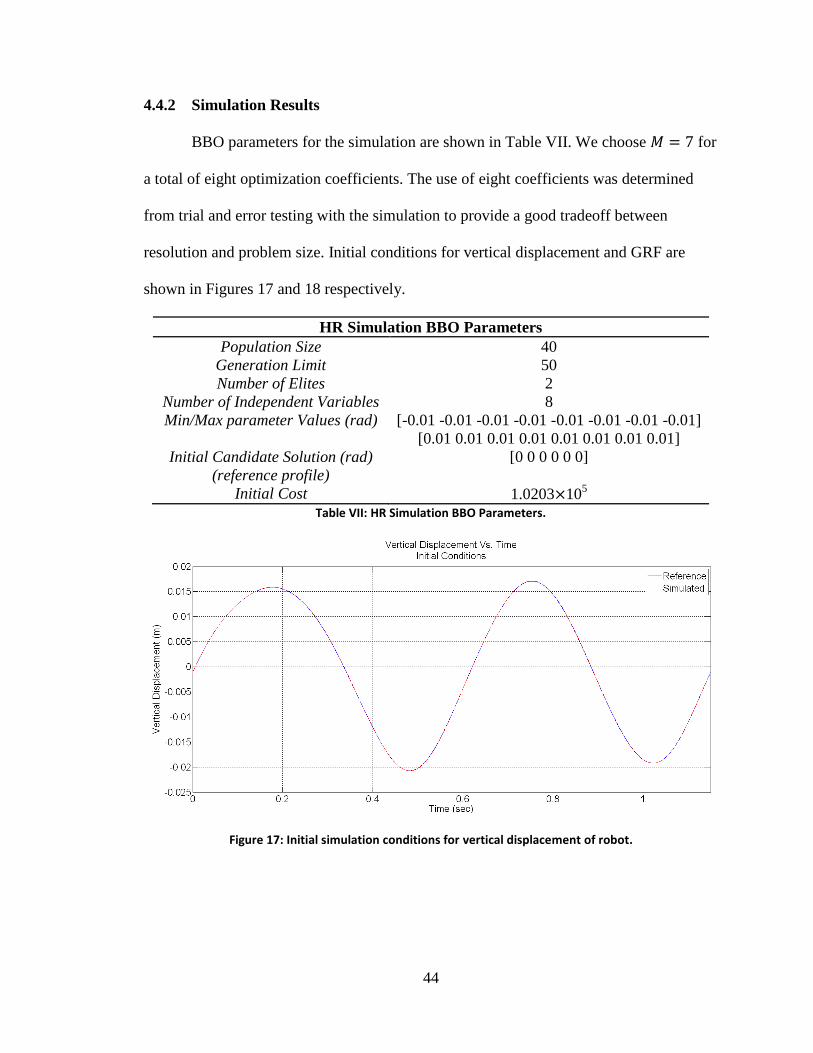
BBO parameters for the simulation are shown in Table VII. We choose for

a total of eight optimization coefficients. The use of eight coefficients was determined

from trial and error testing with the simulation to provide a good tradeoff between

resolution and problem size. Initial conditions for vertical displacement and GRF are

shown in Figures 17 and 18 respectively.

HR Simulation BBO Parameters

Population Size 40

Generation Limit 50

Number of Elites 2

Number of Independent Variables 8

Min/Max parameter Values (rad) [-0.01 -0.01 -0.01 -0.01 -0.01 -0.01 -0.01 -0.01]

[0.01 0.01 0.01 0.01 0.01 0.01 0.01 0.01]

Initial Candidate Solution (rad)

(reference profile)

[0 0 0 0 0 0]

Initial Cost 1.0203 105

Table VII: HR Simulation BBO Parameters.

Figure 17: Initial simulation conditions for vertical displacement of robot.

45

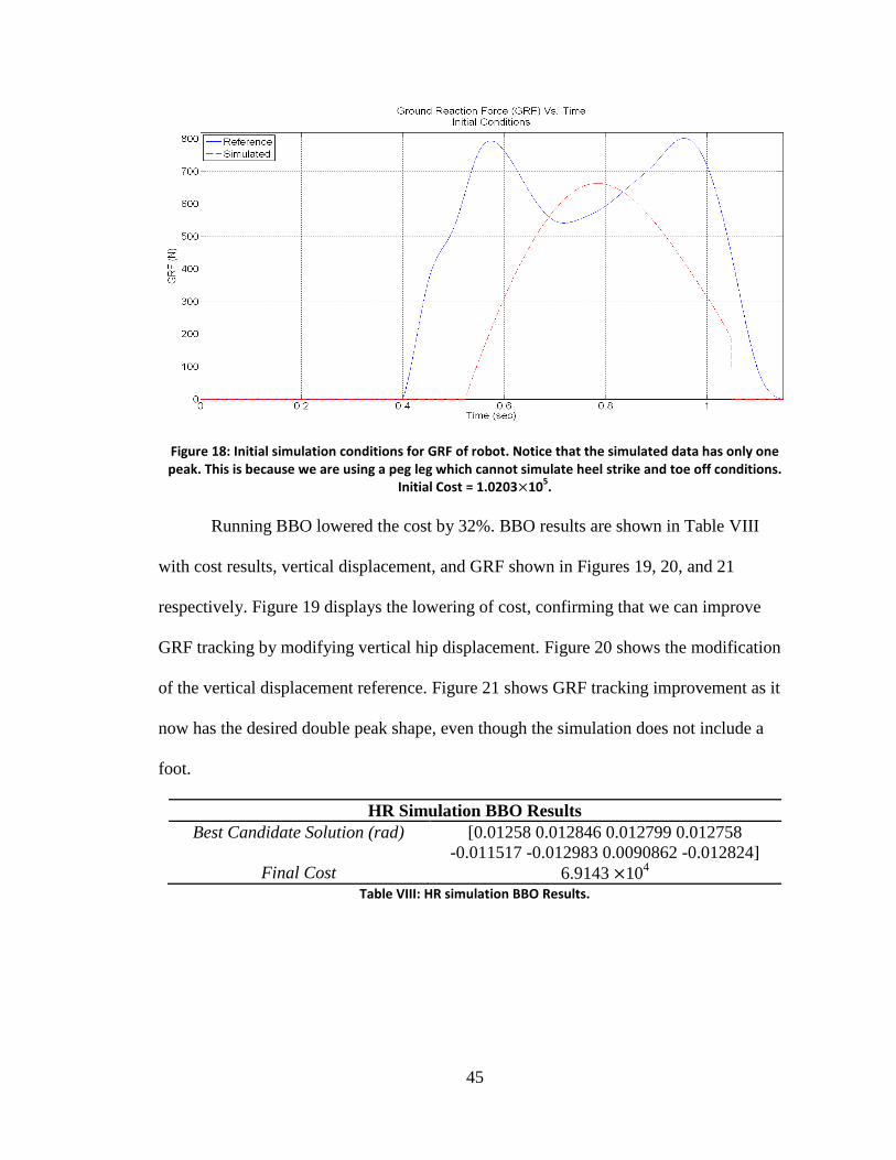
Figure 18: Initial simulation conditions for GRF of robot. Notice that the simulated data has only one peak. This is because we are using a peg leg which cannot simulate heel strike and toe off conditions.

Initial Cost = 1.0203 105.

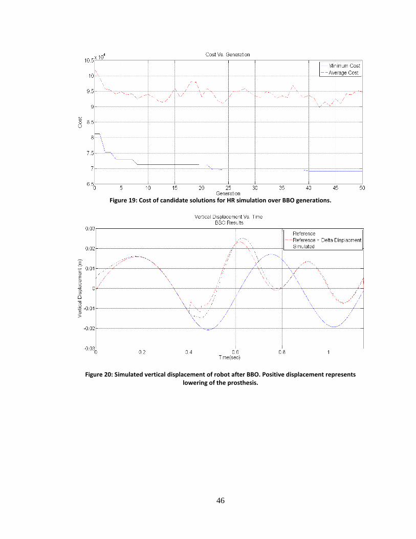
Running BBO lowered the cost by 32%. BBO results are shown in Table VIII

with cost results, vertical displacement, and GRF shown in Figures 19, 20, and 21

respectively. Figure 19 displays the lowering of cost, confirming that we can improve

GRF tracking by modifying vertical hip displacement. Figure 20 shows the modification

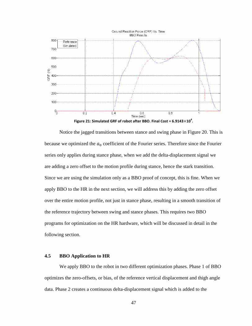
of the vertical displacement reference. Figure 21 shows GRF tracking improvement as it

now has the desired double peak shape, even though the simulation does not include a

foot.

HR Simulation BBO Results

Best Candidate Solution (rad) [0.01258 0.012846 0.012799 0.012758

-0.011517 -0.012983 0.0090862 -0.012824]

Final Cost 6.9143 104

Table VIII: HR simulation BBO Results.

46

Figure 19: Cost of candidate solutions for HR simulation over BBO generations.

Figure 20: Simulated vertical displacement of robot after BBO. Positive displacement represents lowering of the prosthesis.

47

Figure 21: Simulated GRF of robot after BBO. Final Cost = 6.9143 10

4.

Notice the jagged transitions between stance and swing phase in Figure 20. This is

because we optimized the coefficient of the Fourier series. Therefore since the Fourier

series only applies during stance phase, when we add the delta-displacement signal we

are adding a zero offset to the motion profile during stance, hence the stark transition.

Since we are using the simulation only as a BBO proof of concept, this is fine. When we

apply BBO to the HR in the next section, we will address this by adding the zero offset

over the entire motion profile, not just in stance phase, resulting in a smooth transition of

the reference trajectory between swing and stance phases. This requires two BBO

programs for optimization on the HR hardware, which will be discussed in detail in the

following section.

4.5 BBO Application to HR

We apply BBO to the robot in two different optimization phases. Phase 1 of BBO

optimizes the zero-offsets, or bias, of the reference vertical displacement and thigh angle

data. Phase 2 creates a continuous delta-displacement signal which is added to the

48

vertical displacement reference. The delta-displacement signal is created and represented

using the same methods as used for the HR simulation. Phase 1 and phase 2 are discussed

in more detail in Sections 4.5.1 and 4.5.2 respectively. Here we present concepts which

apply to both optimization programs.

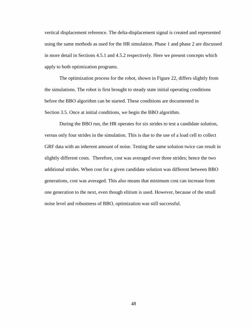
The optimization process for the robot, shown in Figure 22, differs slightly from

the simulations. The robot is first brought to steady state initial operating conditions

before the BBO algorithm can be started. These conditions are documented in

Section 3.5. Once at initial conditions, we begin the BBO algorithm.

During the BBO run, the HR operates for six strides to test a candidate solution,

versus only four strides in the simulation. This is due to the use of a load cell to collect

GRF data with an inherent amount of noise. Testing the same solution twice can result in

slightly different costs. Therefore, cost was averaged over three strides; hence the two

additional strides. When cost for a given candidate solution was different between BBO

generations, cost was averaged. This also means that minimum cost can increase from

one generation to the next, even though elitism is used. However, because of the small

noise level and robustness of BBO, optimization was still successful.

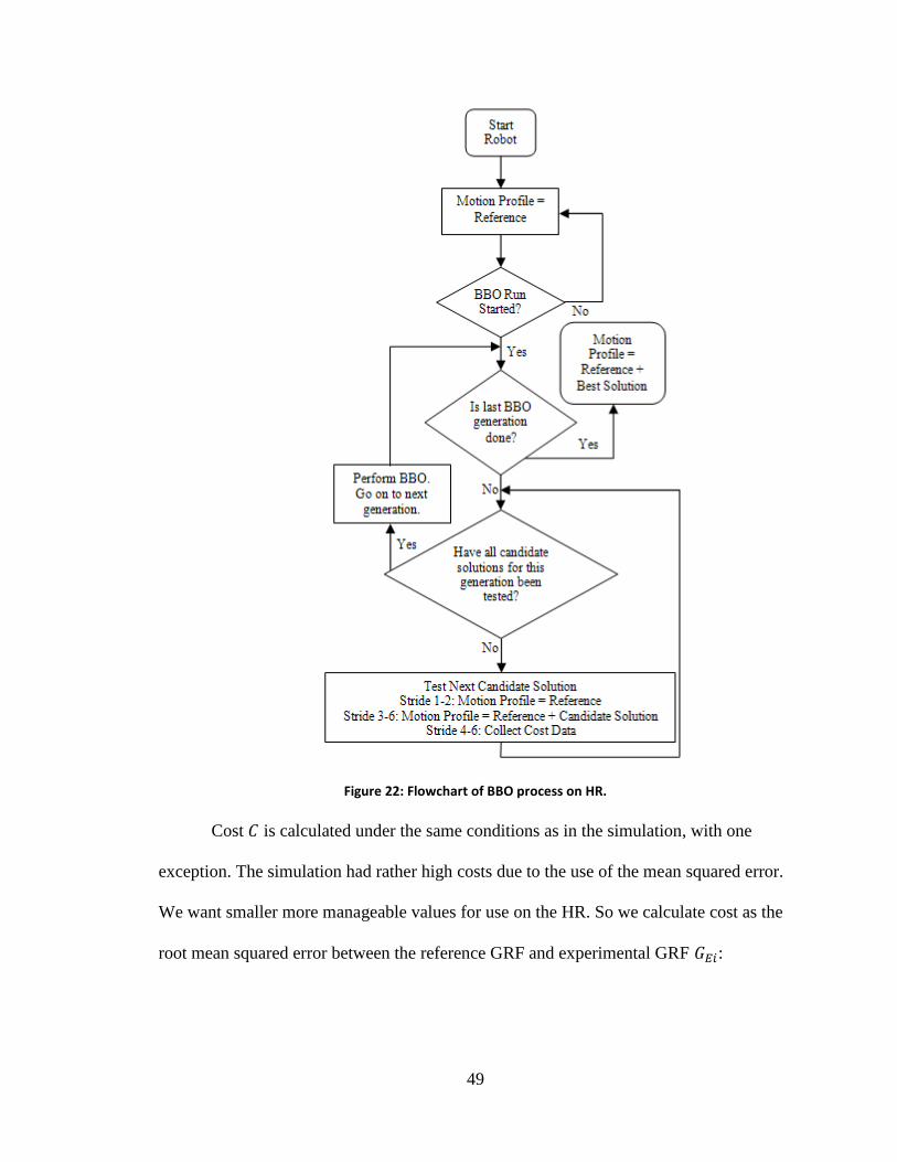
49

Figure 22: Flowchart of BBO process on HR.

Cost is calculated under the same conditions as in the simulation, with one

exception. The simulation had rather high costs due to the use of the mean squared error.

We want smaller more manageable values for use on the HR. So we calculate cost as the

root mean squared error between the reference GRF and experimental GRF :

50

(4.5)

4.5.1 Phase 1: Bias BBO

As seen previously in simulation, varying in the Fourier series representation

of the delta-displacement signal caused unwanted discontinuity between stance and swing

phases. Rather than biasing the vertical displacement signal by means of , we bias the

signal over the entire stride separately from the Fourier series.

During initial testing of the HR, bias of both reference trajectories was varied

manually to observe its effects on GRF. GRF was very sensitive to both zero-offsets of

the reference data. Varying thigh angle bias changed the heel strike and toe off conditions

in the GRF profile. Adjusting the vertical displacement offset modified the magnitude of

the HR’s GRF. We therefore choose to optimize both zero-offsets.

Unlike BBO as applied in the simulation and later in phase 2, bias BBO in

phase 1 is applied across the entire stride rather than just in stance phase. Therefore, bias

is updated at the beginning of each stride rather than at the start of stance phase.

Optimization could not be completed using one BBO run because of the small

safe operating ranges of the robot. Generally, both thigh-angle bias and vertical-

displacement bias are lowered to achieve a better GRF. However if one of these values

was lowered too far, the HR would enter an unsafe operating condition. To remain in safe

operation both values must be lowered together. To accomplish this, a set of two BBO

runs were completed. We refer to these as phases 1.1 and 1.2.

To determine the initial safe search space, the HR was first brought to normal

operating conditions (zero biases). Thigh angle bias and vertical displacement bias were

51

then adjusted manually until the limits of the HR were approached. Search space

parameters were determined using the same method for phase 1.2. However, the robot

was initially brought to the biases determined in phase 1.1 instead of normal operating

conditions.

Initial conditions and parameters for both bias BBO phases are shown in

Table IX. Note that the initial candidate solution for phase 1.2 is not contained

within the min/max parameter values. The initial population in phase 1.2 is random and

therefore possible to contain poor candidate solutions. We test the initial condition from

phase 1.1 to verify the improvement in phase 1.2.

Bias BBO Parameters

Both Phases Population Size 10

Generation Limit 12

Number of Elites 2

Number of Independent

Variables

2

Initial Candidate Solution

(rad)

[0 0]

Initial Cost 390.75

Phase 1.1 Min/Max parameter

Values (rad)

[-0.1300 0.0000]

[0.0000 2.400]

Best Candidate Solution

(rad)

[-0.1299 2.3757]

Best Cost 251.54

Phase 1.2 Min/Max parameter

Values (rad)

[-0.1300 2.0265]

[0.1183 5.5000]

Best Candidate Solution

(rad)

[-0.1253 4.8170]

Best Cost 197.61

Table IX: Bias BBO (Phase 1) parameters as applied to the HR.

Results for the bias optimization runs are also shown in Table IX. Phases 1.1 and

1.2 took approximately 14 minutes each to run on the hardware. Convergence results are

shown in Figure 23. Cost was lowered to in phase 1.1 and lowered further to

in phase 1.2. Overall reduction in cost is 49% from the initial condition.

Robot operation with the biased signals and resultant GRFs are shown in Figures 24, 25,

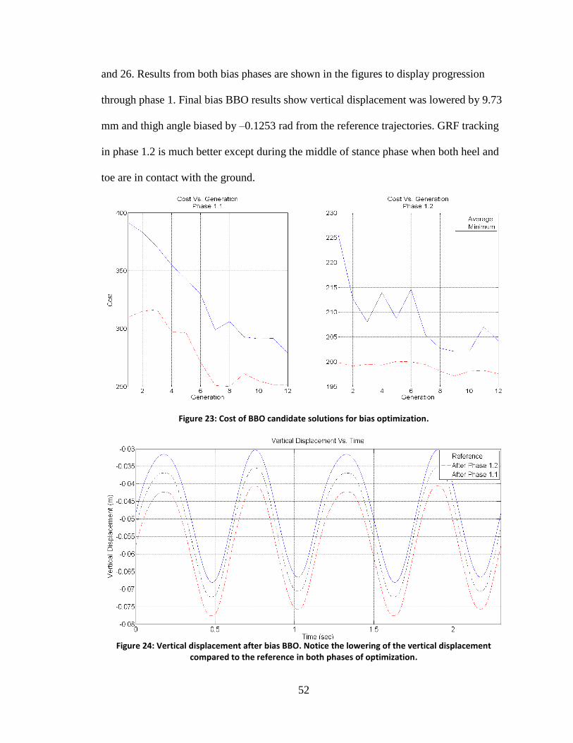
52

and 26. Results from both bias phases are shown in the figures to display progression

through phase 1. Final bias BBO results show vertical displacement was lowered by 9.73

mm and thigh angle biased by –0.1253 rad from the reference trajectories. GRF tracking

in phase 1.2 is much better except during the middle of stance phase when both heel and

toe are in contact with the ground.

Figure 23: Cost of BBO candidate solutions for bias optimization.

Figure 24: Vertical displacement after bias BBO. Notice the lowering of the vertical displacement

compared to the reference in both phases of optimization.

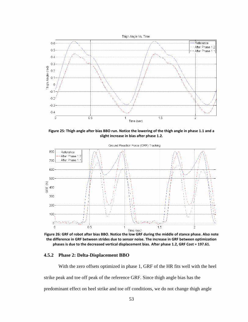
53

Figure 25: Thigh angle after bias BBO run. Notice the lowering of the thigh angle in phase 1.1 and a slight increase in bias after phase 1.2.

Figure 26: GRF of robot after bias BBO. Notice the low GRF during the middle of stance phase. Also note

the difference in GRF between strides due to sensor noise. The increase in GRF between optimization phases is due to the decreased vertical displacement bias. After phase 1.2, GRF Cost = 197.61.

4.5.2 Phase 2: Delta-Displacement BBO

With the zero offsets optimized in phase 1, GRF of the HR fits well with the heel

strike peak and toe off peak of the reference GRF. Since thigh angle bias has the

predominant effect on heel strike and toe off conditions, we do not change thigh angle

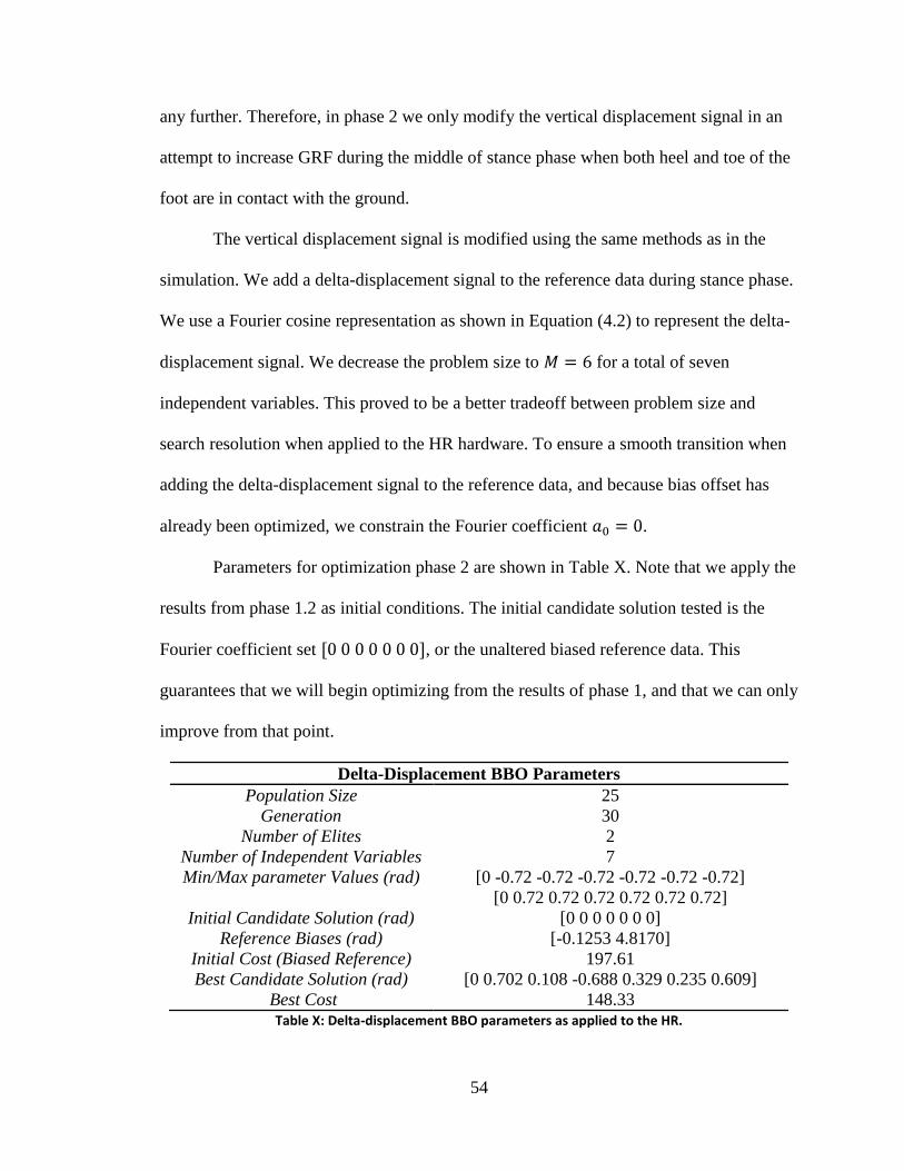
54

any further. Therefore, in phase 2 we only modify the vertical displacement signal in an

attempt to increase GRF during the middle of stance phase when both heel and toe of the

foot are in contact with the ground.

The vertical displacement signal is modified using the same methods as in the

simulation. We add a delta-displacement signal to the reference data during stance phase.

We use a Fourier cosine representation as shown in Equation (4.2) to represent the delta-

displacement signal. We decrease the problem size to for a total of seven

independent variables. This proved to be a better tradeoff between problem size and

search resolution when applied to the HR hardware. To ensure a smooth transition when

adding the delta-displacement signal to the reference data, and because bias offset has

already been optimized, we constrain the Fourier coefficient .

Parameters for optimization phase 2 are shown in Table X. Note that we apply the

results from phase 1.2 as initial conditions. The initial candidate solution tested is the

Fourier coefficient set , or the unaltered biased reference data. This

guarantees that we will begin optimizing from the results of phase 1, and that we can only

improve from that point.

Delta-Displacement BBO Parameters

Population Size 25

Generation 30

Number of Elites 2

Number of Independent Variables 7

Min/Max parameter Values (rad) [0 -0.72 -0.72 -0.72 -0.72 -0.72 -0.72]

[0 0.72 0.72 0.72 0.72 0.72 0.72]

Initial Candidate Solution (rad) [0 0 0 0 0 0 0]

Reference Biases (rad) [-0.1253 4.8170]

Initial Cost (Biased Reference) 197.61

Best Candidate Solution (rad) [0 0.702 0.108 -0.688 0.329 0.235 0.609]

Best Cost 148.33 Table X: Delta-displacement BBO parameters as applied to the HR.

55

Results of the BBO run are shown in Table X, with performance shown in

Figure 27. Phase 2 took approximately 1 hour and 20 minutes to run on the robot

hardware. BBO lowered the cost to , or by 62% from the reference data.

Figure 28 shows the modified vertical displacement signal compared to the original

reference data and the biased initial conditions. We show the biased vertical displacement

to demonstrate the effect of the delta-displacement signal. Thigh angle is the same as

phase 1.2 as shown in Figure 25. The improved GRF profile is shown in Figure 29,

effectively showing the robot compensating for the prosthesis.

Figure 27: Cost of BBO candidate solutions for delta-displacement optimization.

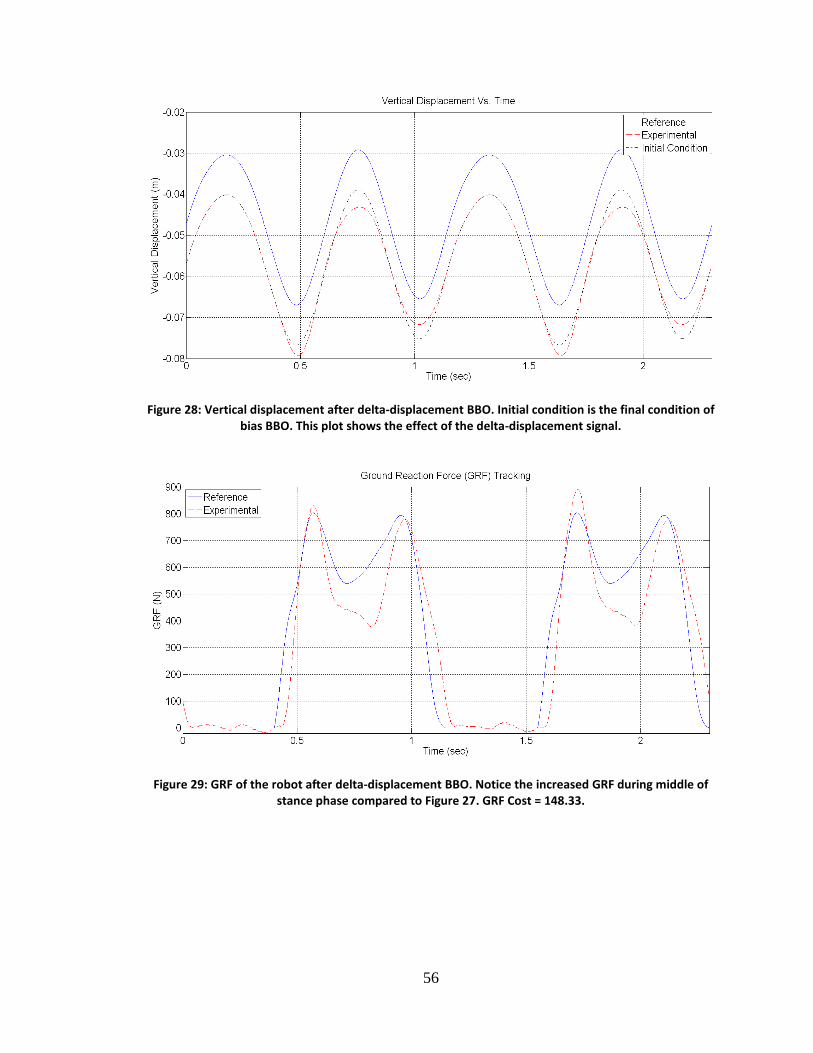
56

Figure 28: Vertical displacement after delta-displacement BBO. Initial condition is the final condition of bias BBO. This plot shows the effect of the delta-displacement signal.

Figure 29: GRF of the robot after delta-displacement BBO. Notice the increased GRF during middle of stance phase compared to Figure 27. GRF Cost = 148.33.

57

CHAPTER V

CONCLUSION

5.1 Summary

We have discussed and summarized problems associated with the testing of

prostheses on human subjects. We propose the use of a HR to facilitate prosthesis testing.

The HR emulates the movements of a human hip and allows prostheses to be tested under

conditions not possible with human subjects.

We use feedback control on the HR to track the human hip motions used as

references. Thigh angle and vertical displacement are tracked. We develop SMCs for

both drive stages in order to track reference inputs. Results show exceptional tracking of

both drive stages.

The hip motions used as references are shown to have limitations due to

discontinuities in the derivatives. Because SMC requires smoothness of the reference

signal and its first two derivatives, we adjust the reference data accordingly. We apply a

spline-based smoothing algorithm to optimize the data so that SMC can be used without

any problems with derivative discontinuities.

58

We apply BBO to control the GRF of the robot. We modify the reference hip

motions using BBO to simulate a prosthesis user compensating for a prosthesis. A

simulation of the HR is used to design test procedures for the HR. Using the simulation,

we also confirm the feasibility of modifying vertical hip displacement of the HR in order

to improve GRF tracking.

Applying BBO to the HR required two distinct optimization programs. We first

optimized bias for both thigh angle and vertical displacement reference data. Next a

delta-displacement signal was added to the reference vertical displacement data to modify

the reference data further. The delta-displacement signal was optimized using BBO.

Results show a 62% improvement in GRF tracking of the HR as compared to that

obtained with the original reference gait data.

5.2 Future Work

To improve the results shown here and make these tests more applicable to other

prostheses, a few things need to be adapted. Generally, when BBO is used, it would be

applied for many generations – for example, up to 100,000 generations in [5]. While that

would be unfeasible with the robot, a modest increase from this thesis would be an

improvement. Due to the time demands of these tests, including taking six strides per

candidate solution, the robot was only run for a maximum of 30 generations at a time.

Lowering the number of strides to test a solution would allow an increase in the number

of generations. We could lower the number of necessary strides by designing a new GRF

measurement system, or perhaps by purchasing a load cell with less noise.

In the results, GRF of the robot/prosthesis combination always had a small time

delay compared to the desired signal. Adding the delta-displacement signal to the

59

reference trajectory was always done during the stance phase as defined by the reference

data. Since we are modifying the reference data in order to improve GRF, we could allow

a slight time shift when adding the delta-displacement signal when it is added to the

reference data.

When applying BBO, the real-time derivative of the delta displacement signal

added to the reference data was calculated using a low pass filter approximation for input

to SMC. This was done for ease of coding. We could avoid this approximation by

calculating the derivatives of the Fourier series representing the delta-displacement

signal. The derivatives of the delta-displacement signal could then be added to the

corresponding derivatives of the reference data, avoiding the need for a real time

approximation.

Finally, we would like to adapt these tests and apply them to other prostheses.

60

REFERENCES

[1] A. Shah, Distributed Biogeography Based Optimization for Mobile Robots,

Master’s Thesis, Cleveland State University, Cleveland, OH, 2009.

[2] A. van den Bogert, S. Samorezov, B. Davis, and W. Smith, “Modeling and

Optimal Control of an Energy-Storing Prosthetic Knee,” Journal of

Biomechanical Engineering, vol. 134, no. 5, pp. 0510071-0510078, 2012.

[3] A. Segal, M. Orenduff, G. Klute, M. McDowell, J. Pecoraro, J. Shofer, and J.

Czerniecki, “Kinematic and Kinetic Comparisons of Transfemoral Amputee

Gait Using C-Leg and Mauch SNS® Prosthetic Knees,” Journal of

Rehabilitation Research and Development, vol. 43, no. 7, pp. 857-870, 2006.

[4] C. Lin, P. Chang, and J. Luh, “Formulation and Optimization of Cubic

Polynomial Joint Trajectories for Industrial Robots,” IEEE Transactions on

Automatic Control, vol. AC-28, no. 12, pp. 1066-1073, 1983.

[5] D. Sadey, Parameter Identification for the generation of Dynamic

Electrocardiograms, Honor’s Thesis, Cleveland State University, Cleveland,

OH, 2012.

[6] D. Simon, “Biogeography-Based Optimization,” IEEE Transactions on

Evolutionary Computation, vol. 12, no. 6, pp. 702-713, 2008.

[7] D. Simon, Evolutionary Optimization Algorithms, John Wiley & Sons, 2013.

[8] D. Simon and C. Isik, “The Generation and Optimization of Trigonometric

Joint Trajectories for Robotic Manipulators,” Proceedings of the American

Control Conference, Boston, MA, pp. 2027-2032, 1991.

61

[9] D. Simon and C. Isik, “Optimal Trigonometric Robot Joint Trajectories,”

Robotica, vol. 9, pp. 379-386, 1991.

[10] D. Simon, “Optimal Robot Motions for Repetitive Tasks,” Proceedings of the

31st Conference on Decision and Control, Tucson, AZ, pp. 3130-3134, 1992

[11] D. Winter, Biomechanics and Motor Control of Human Gait, 2nd

Edition,

University of Waterloo Press, 1991.

[12] F. Sup, A. Bohara, and M. Goldfarb, “Design and Control of a Powered Knee

and Ankle Prosthesis: Initial Evaluation on a Transfemoral Amputee,” IEEE

International Conference on Robotics and Automation, Rome, Italy, pp. 4134-

4139, 2007.

[13] F. Sup, A. Bohara, and M. Goldfarb, “Design and Control of a Powered

Transfemoral Prosthesis,” The International Journal of Robotics Research,

vol. 27, no. 2, pp. 263-273, 2008.

[14] F. Sup, H. Atakan, J. Mitchell, T. Withrow, and M. Goldfarb, “Design and

Control of an Active Electrical Knee and Ankle Prosthesis,” IEEE RAS EMBS

International Conference on Biomedical Robotics and Biomechatronics,

Scottsdale, AZ, pp. 523-528, 2008.

[15] F. Sup, H. Atakan, J. Mitchell, T. Withrow, and M. Goldfarb, “Self-Contained

Powered Knee and Ankle Prosthesis: Initial Evaluation on a Transfemoral

Amputee,” IEEE International Conference on Rehabilitation Robotics, Kyoto,

Japan, pp. 638-644, 2009.

62

[16] G. Konidaris, S. Osentoski, and P. Thomas. “Value function approximation in

reinforcement learning using the Fourier basis,” Twenty-Fifth Conference on

Artificial Intelligence, San Francisco, California, pp. 1468-1473, 2011.

[17] G. Nandi, A. Ijspeert, P. Chakraborty, and A. Nandi, “Development of

Adaptive Modular Active Leg (AMAL) Using Bipedal Robotics Technology,”

Robotics and Autonomous Systems, vol. 57, no. 6, pp. 603-616, 2009.

[18] G. Thomas, T. Wilmot, S. Szatmary, D. Simon, and W. Smith, “Evolutionary

Optimization of Artificial Neural Networks for Prosthetic Knee Control,”

Efficiency and Scalability Methods for Computational Intellect, (B. Igelnik

and J. Zurada, editors), Chap. 7, pp. 142-161, IGI Global, 2013.

[19] H. Richter, Advanced Control of Turbofan Engines, Springer Science +

Business Media, 2012.

[20] H. Richter and D. Simon, “Robust Tracking Control of a Prosthesis Test

Robot”, to appear in ASME Journal of Dynamic Systems, 2014.

[21] I. Pappas, M. Popovic, T. Keller, V. Dietz, and M. Morari, “A Reliable Gait

Phase Detection System,” IEEE Transactions on Neural Systems and

Rehabilitation Engineering, vol. 9, no. 2, pp. 113-125, 2001.

[22] J. Johansson, D. Sherrill, P. Riley, P. Bonato, and H. Herr, “A Clinical

Comparison of Variable-Damping and Mechanically Passive Prosthetic Knee

Devices,” American Journal of Physical Medicine & Rehabilitation, vol. 84,

no. 8, pp. 563-575, 2005.

[23] K. Zemalache, M. Tahar, A. Omari, and H. Maaref, “Sliding Mode Control

Technique: Application to a Four Rotors Mini-Flying Robot,” Intelligent

63

Systems and Automation, 2nd

Mediterranean Conference, vol. 1107, no. 1, pp.

160-165, 2009.

[24] L. Graham, D. Datta, B. Heller, and J. Howitt, “A Comparative Study of

Conventional and Energy-Storing Prosthetic Feet in High-Functioning

Transfemoral Amputees,” Archives of Physical Medicine & Rehabilitation,

vol. 88, no. 7, pp. 801-806, 2007.

[25] M. Bellman, T. Schmalz, and S. Blumentritt, “Comparative Biomechanical

Analysis of Current Microprocessor-Controlled Prosthetic Knee Joints,”

Archives of Physical Medicine & Rehabilitation, vol. 91, no. 4, pp. 644-652,

2010.

[26] N. Ghani, N. Yatim, and N. Azmi, “Trajectory Tracking of Two Wheels

Mobile Robot Using Sliding Mode Control,” Proceedings of the Fourth

Global Conference on Power Control and Optimization, vol. 1337, no. 1, pp.

135-139, 2011.

[27] P. A. Lilley, M. Raine, and G.W. Blunn, “In Vitro Generation of Replacement

Knee Wear by Simulation,” Proceedings of International Conference on

Simulation, York, UK, pp. 35-41, 1998.

[28] P. A. Lilley, M. Raine, and G.W. Blunn, “Simulation of the Wear of Metal

Implants by Soft-Tissue,” Proceedings of International Conference on

Simulation, York, UK, pp. 42-49, 1998.

[29] R. Davis, H. Richter, D. Simon, and A. van den Bogert, “Evolutionary

Optimization of Ground Reaction Force for a Prosthetic Leg Testing Robot,”

Submitted to the American Control Conference 2014 for publication.

64

[30] R. Gailey, K. Allen, J. Castles, J. Kucharik, and M. Roeder, “Review of

Secondary Physical Conditions Associated with Lower-Limb Amputation and

Long-Term Prosthesis Use,” Journal of Rehabilitation & Development, vol.

45, no. 1, pp. 15-20, 2008.

[31] R. Robinson, C. Kothera, B. Woods, R. Vocke, and N. Wereley, “High

Specific Power Actuators for Robotic Manipulators,” Journal of Intelligent

Material Systems and Structures, vol. 22, no. 13, pp. 1501-1511, 2011.

[32] R. Williams, A. Turner, M. Orenduff, A. Segal, G. Klute, J. Pecoraro, and J.

Czerniecki, “Does Having a Computerized Prosthetic Knee Influence

Cognitive Performance During Amputee Walking?” Archives of Physical

Medicine & Rehabilitation, vol. 87, no. 7, pp. 989-994, 2006.

[33] S. Au, P. Bonato, and H. Herr, “An EMG-Postion Controlled System for an

Active Ankle-Foot Prosthesis: An Initial Experimental Study,” Proceedings of

the 2005 IEEE International Conferecne on Rehabilitation Robotics, Chicago,

IL, pp. 375-379, 2005.

[34] S. Chand and K. Doty, “On-Line Polynomial Trajectories for Robot

Manipulators,” The International Journal of Robotics Research, vol. 4, no. 2,

pp. 38-48, 1985.

[35] S. Thompson and R. Patel, “Formulation of Joint Trajectories for Industrial

Robots Using B-Splines,” IEEE Transactions on Industrial Electronics, vol.

IE-34, no. 2, pp. 192-199, 1987.

[36] T. Bae, K. Choi, D. Hong, and M. Mun, “Dynamic Analysis of Above-Knee

Amputee Gait,” Clinical Biomechanics, vol. 22, no. 5, pp. 557-566, 2006.

65

[37] T. Chin, K. Machida, S. Sawamura, R. Shiba, H. Oyabu, Y. Nagakura, I.

Takase, and A. Nakagawa, “Comparison of Different Microprocessor

Controlled Knee Joints on the Energy Consumption During Walking in Trans-

Femoral Amputees: Intelligent Knee Prosthesis (IP) versus C-Leg,”

Prosthetics and Orthotics International, vol. 30, no. 1, pp. 73-80, 2006.

[38] T. Wilmot, G. Thomas, B. Montavon, R. Rarick, A. van den Bogert, S.

Szatmary, D. Simon, W. Smith, and S. Samorezov, “Biogeography-Based

Optimization for Hydraulic Prosthetic Knee Control,” Medical Cyber-

Physical Systems Workshop, Philadelphia, PA, pp. 18-25, 2013.

[39] T. Wilmot, Intelligent Controls for a Semi-Active Hydraulic Prosthetic Knee,

Master’s Thesis, Cleveland State University, Cleveland, OH, 2011.

[40] W. Dyck, S. Onyshko, D. Hobson, D. Winter, and A. Quanbury, “A

Voluntarily Controlled Electrohydraulic Above-Knee Prosthesis,” Bullettin of

Prosthetics Research, vol. 10, no. 23, pp. 169-186, 1975.

[41] X. Yu and O. Kaynak, “Sliding-Mode Control with Soft Computing: A

Survey,” IEEE Transactions on Industrial Electronics, vol. 56, no. 9, pp.

3275-3285, 2009.

[42] 2013, Flex-Foot Feet [Online], Available:

http://www.ossur.com/?PageID=12639

[43] 2013, Mauch Knee [Online], Available:

http://www.ossur.com/?PageID=12644

66

APPENDICES

67

APPENDIX A: Wiring Lists and Schematics

Here the overall wiring lists and schematics are shown for the HR. In order for

proper operation, all wires shown in the following schematics must be connected. The

wiring is broken up into subsections for ease of problem diagnosis. Each list provides

connection information for both ends of a wire as well as color information for any

internal conductor(s) within that wire. An example list is shown below detailing the

content found within each list.

Example Schematic Name

Cable Name

End 1 Main Shielding Color Conductor(s) End 2

Connection Location: Terminal (if needed)

Main color of shielding

for multiple conductor

wires or color of single

conductor

Color of internal

conductors for multiple

conductors or shielding

color for single wires.

Connection Location:

Terminal (if needed)

Acronyms Found in Wiring Lists:

NC Not Connected

LM Linear Motor

TB Terminal Board

RM Rotary Motor

BM Braking Module

CB Control Box

Emg Emergency

MC Microcontroller

QD Quick Disconnect

LC Load Cell

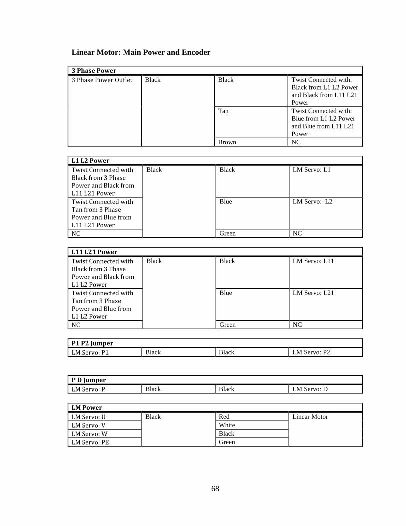
68

Linear Motor: Main Power and Encoder

3 Phase Power 3 Phase Power Outlet Black Black Twist Connected with:

Black from L1 L2 Power

and Black from L11 L21

Power

Tan Twist Connected with:

Blue from L1 L2 Power

and Blue from L11 L21

Power

Brown NC

L1 L2 Power

Twist Connected with Black from 3 Phase Power and Black from L11 L21 Power

Black Black LM Servo: L1

Twist Connected with Tan from 3 Phase Power and Blue from L11 L21 Power

Blue LM Servo: L2

NC Green NC

L11 L21 Power

Twist Connected with Black from 3 Phase Power and Black from L1 L2 Power

Black Black LM Servo: L11

Twist Connected with Tan from 3 Phase Power and Blue from L1 L2 Power

Blue LM Servo: L21

NC Green NC

P1 P2 Jumper

LM Servo: P1 Black Black LM Servo: P2

P D Jumper

LM Servo: P Black Black LM Servo: D

LM Power

LM Servo: U Black Red Linear Motor

LM Servo: V White

LM Servo: W Black

LM Servo: PE Green

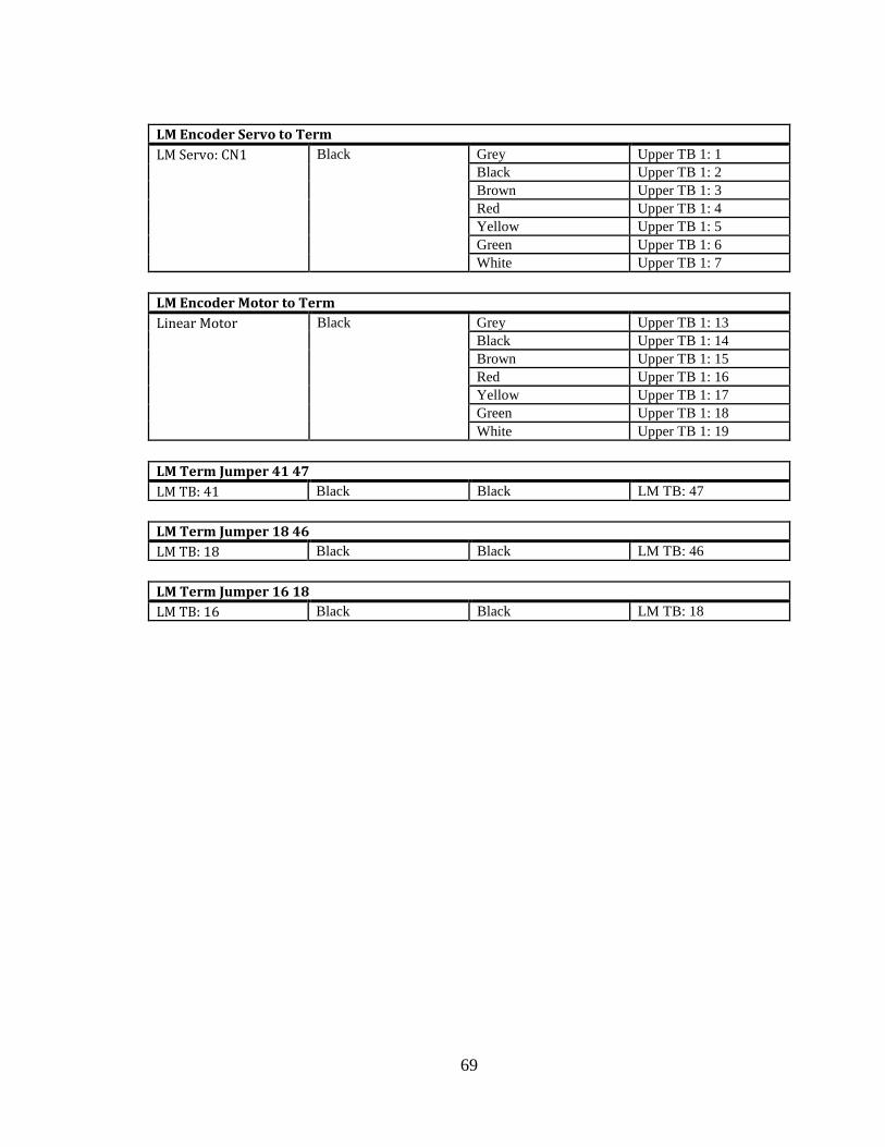
69

LM Encoder Servo to Term

LM Servo: CN1 Black Grey Upper TB 1: 1

Black Upper TB 1: 2

Brown Upper TB 1: 3

Red Upper TB 1: 4

Yellow Upper TB 1: 5

Green Upper TB 1: 6

White Upper TB 1: 7

LM Encoder Motor to Term

Linear Motor Black Grey Upper TB 1: 13

Black Upper TB 1: 14

Brown Upper TB 1: 15

Red Upper TB 1: 16

Yellow Upper TB 1: 17

Green Upper TB 1: 18

White Upper TB 1: 19

LM Term Jumper 41 47

LM TB: 41 Black Black LM TB: 47

LM Term Jumper 18 46

LM TB: 18 Black Black LM TB: 46

LM Term Jumper 16 18

LM TB: 16 Black Black LM TB: 18

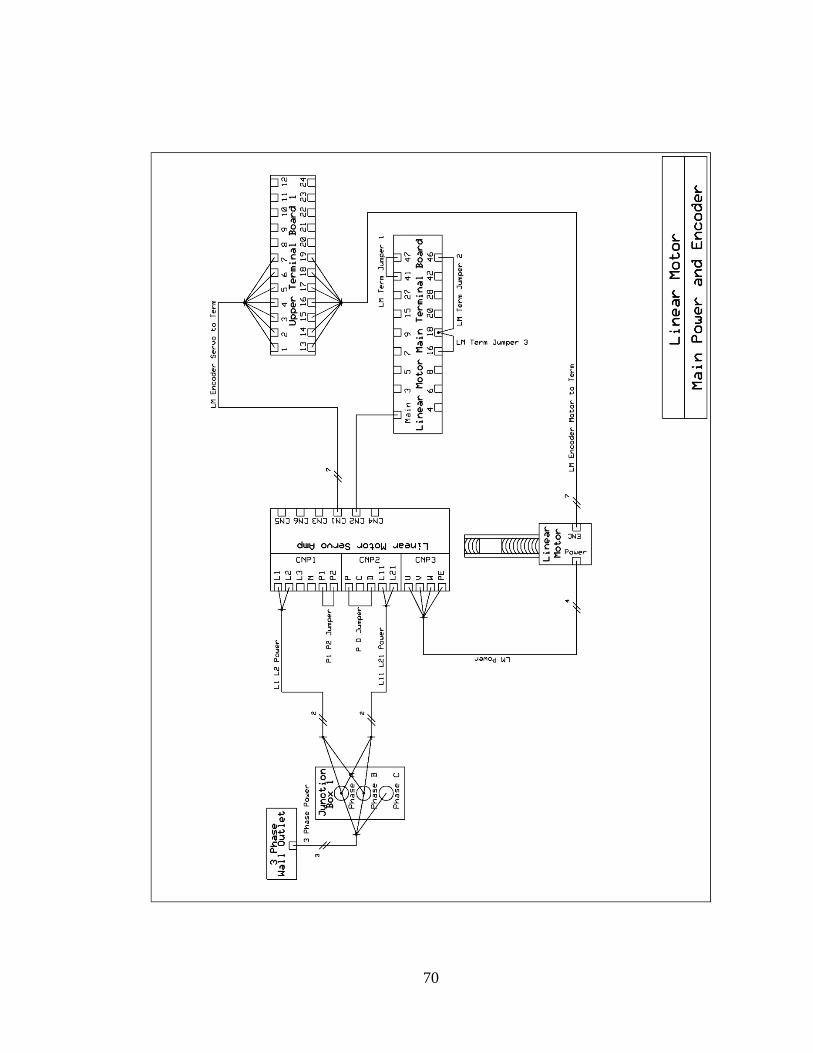
70

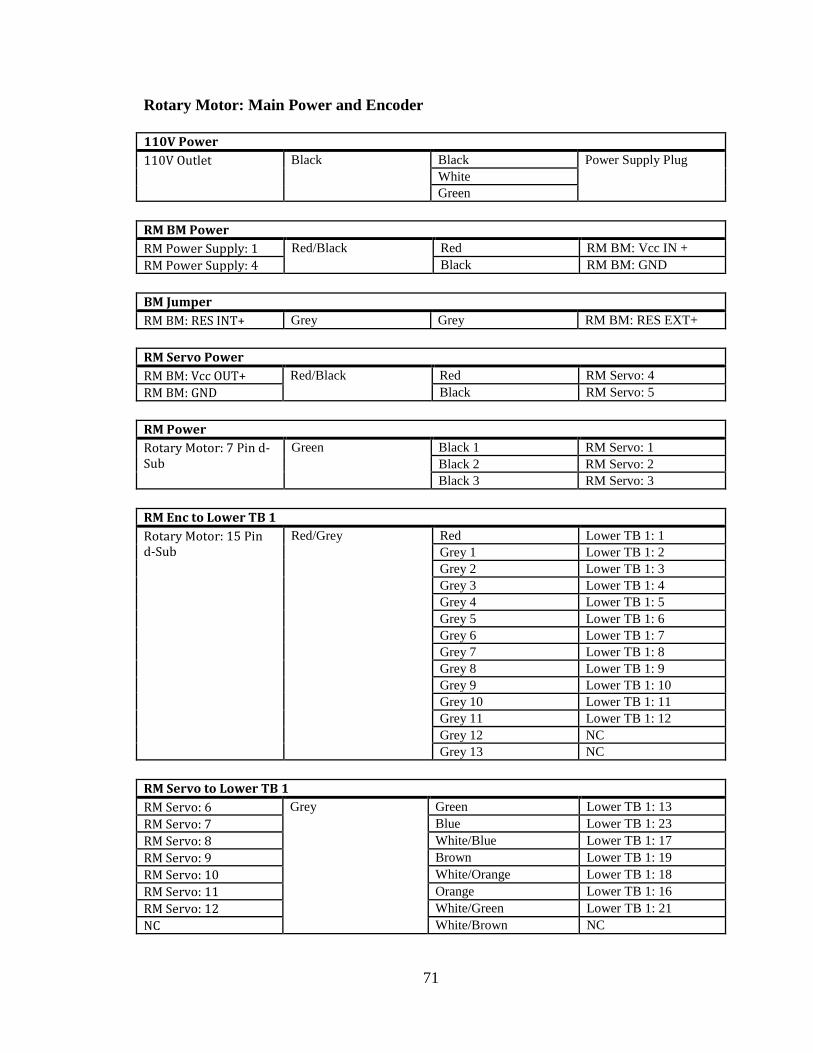
71

Rotary Motor: Main Power and Encoder

110V Power

110V Outlet Black Black Power Supply Plug

White

Green

RM BM Power

RM Power Supply: 1 Red/Black Red RM BM: Vcc IN +

RM Power Supply: 4 Black RM BM: GND

BM Jumper

RM BM: RES INT+ Grey Grey RM BM: RES EXT+

RM Servo Power

RM BM: Vcc OUT+ Red/Black Red RM Servo: 4

RM BM: GND Black RM Servo: 5

RM Power

Rotary Motor: 7 Pin d-Sub

Green Black 1 RM Servo: 1

Black 2 RM Servo: 2

Black 3 RM Servo: 3

RM Enc to Lower TB 1

Rotary Motor: 15 Pin d-Sub

Red/Grey Red Lower TB 1: 1

Grey 1 Lower TB 1: 2

Grey 2 Lower TB 1: 3

Grey 3 Lower TB 1: 4

Grey 4 Lower TB 1: 5

Grey 5 Lower TB 1: 6

Grey 6 Lower TB 1: 7

Grey 7 Lower TB 1: 8

Grey 8 Lower TB 1: 9

Grey 9 Lower TB 1: 10

Grey 10 Lower TB 1: 11

Grey 11 Lower TB 1: 12

Grey 12 NC

Grey 13 NC

RM Servo to Lower TB 1

RM Servo: 6 Grey Green Lower TB 1: 13

RM Servo: 7 Blue Lower TB 1: 23

RM Servo: 8 White/Blue Lower TB 1: 17

RM Servo: 9 Brown Lower TB 1: 19

RM Servo: 10 White/Orange Lower TB 1: 18

RM Servo: 11 Orange Lower TB 1: 16

RM Servo: 12 White/Green Lower TB 1: 21

NC White/Brown NC

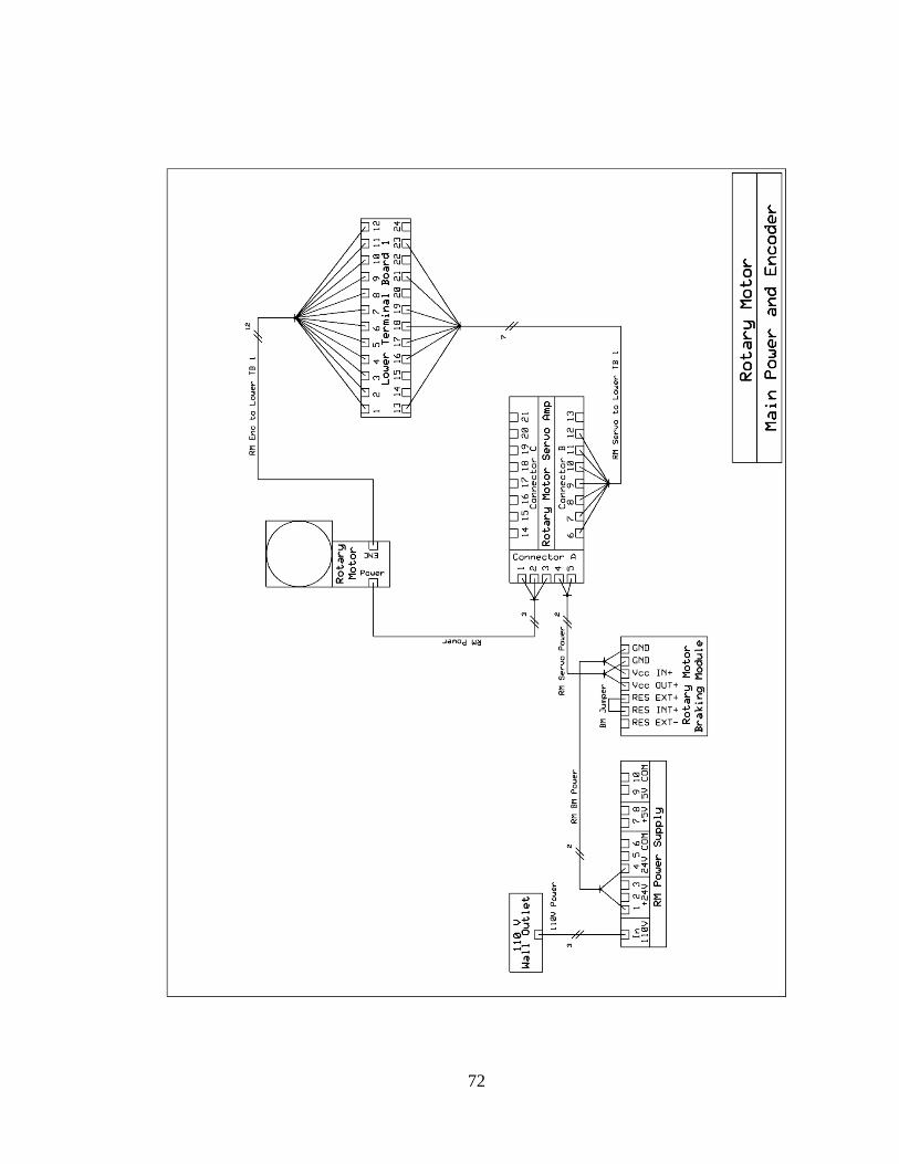
72

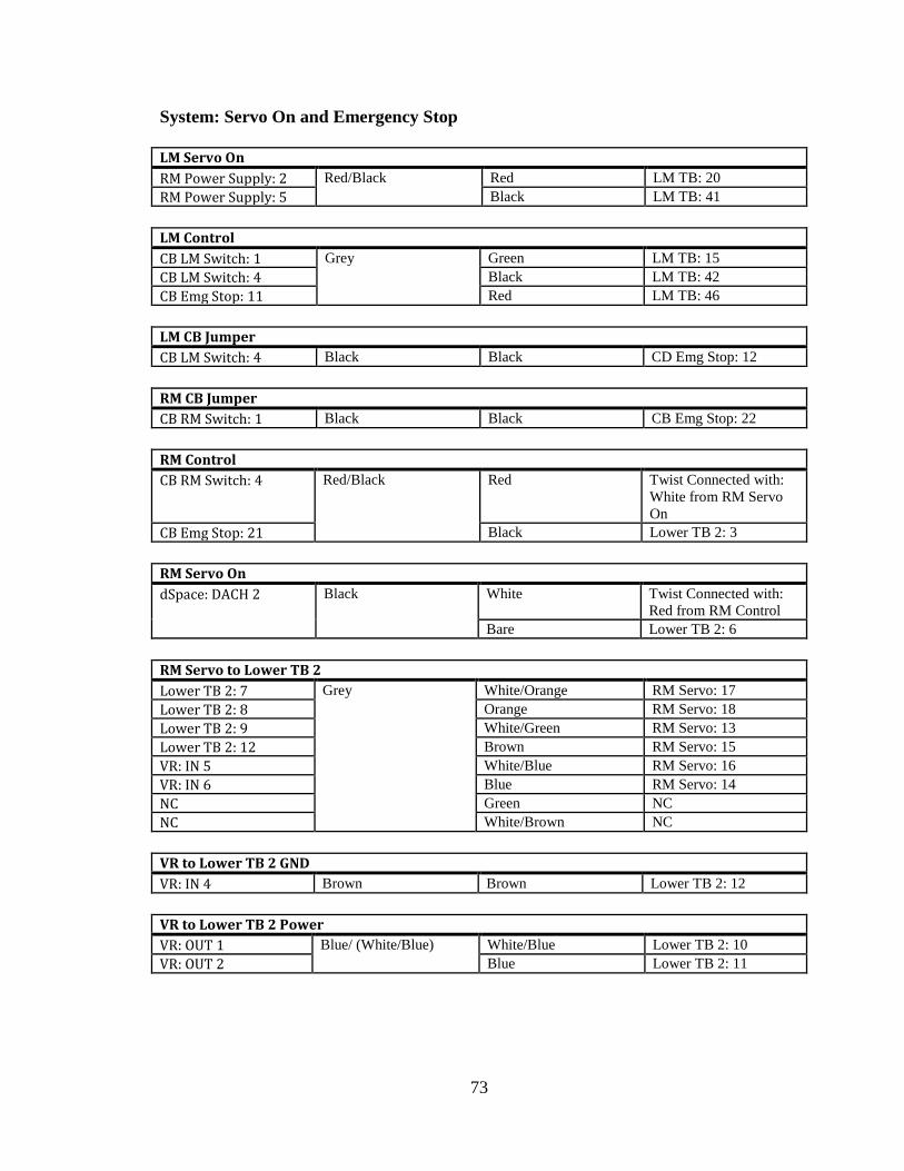
73

System: Servo On and Emergency Stop

LM Servo On

RM Power Supply: 2 Red/Black Red LM TB: 20

RM Power Supply: 5 Black LM TB: 41

LM Control

CB LM Switch: 1 Grey Green LM TB: 15

CB LM Switch: 4 Black LM TB: 42

CB Emg Stop: 11 Red LM TB: 46

LM CB Jumper

CB LM Switch: 4 Black Black CD Emg Stop: 12

RM CB Jumper

CB RM Switch: 1 Black Black CB Emg Stop: 22

RM Control

CB RM Switch: 4 Red/Black Red Twist Connected with:

White from RM Servo

On

CB Emg Stop: 21 Black Lower TB 2: 3

RM Servo On

dSpace: DACH 2 Black White Twist Connected with:

Red from RM Control

Bare Lower TB 2: 6

RM Servo to Lower TB 2

Lower TB 2: 7 Grey White/Orange RM Servo: 17

Lower TB 2: 8 Orange RM Servo: 18

Lower TB 2: 9 White/Green RM Servo: 13

Lower TB 2: 12 Brown RM Servo: 15

VR: IN 5 White/Blue RM Servo: 16

VR: IN 6 Blue RM Servo: 14

NC Green NC

NC White/Brown NC

VR to Lower TB 2 GND

VR: IN 4 Brown Brown Lower TB 2: 12

VR to Lower TB 2 Power

VR: OUT 1 Blue/ (White/Blue) White/Blue Lower TB 2: 10

VR: OUT 2 Blue Lower TB 2: 11

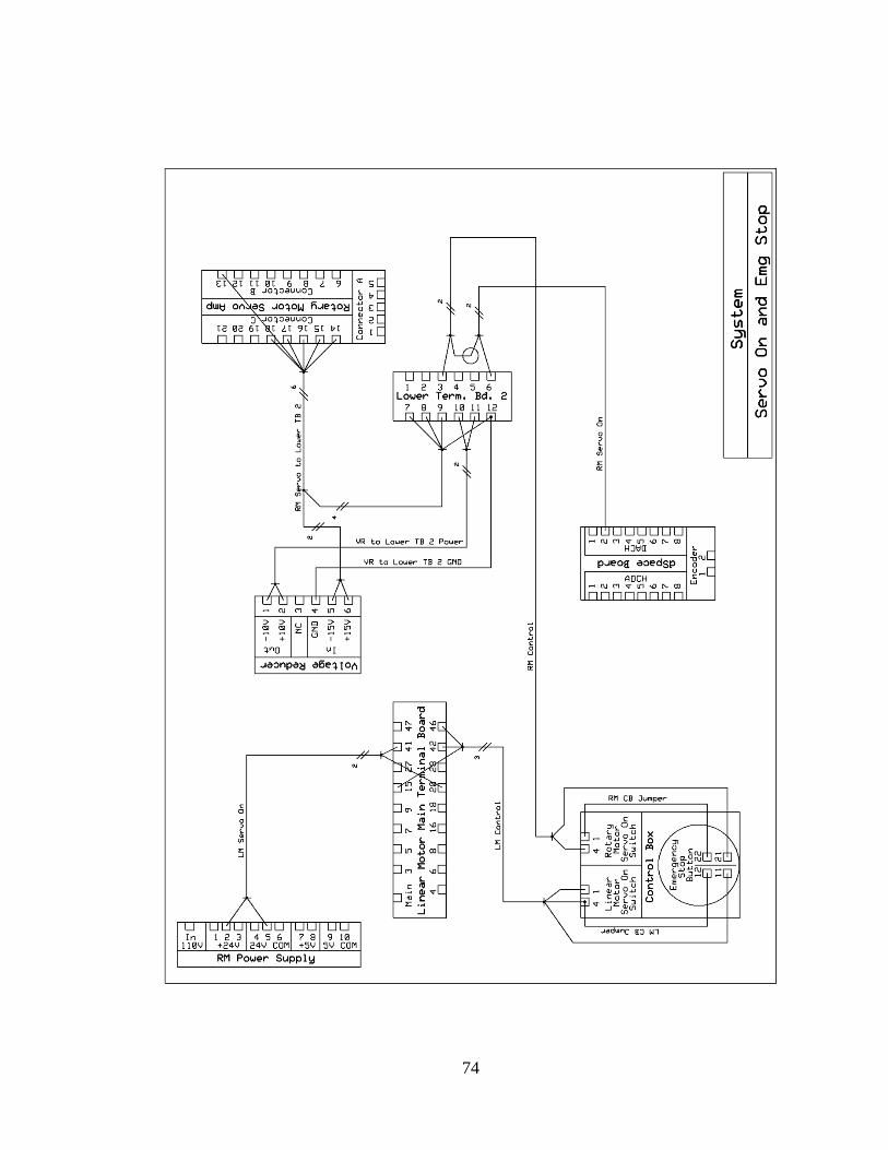
74

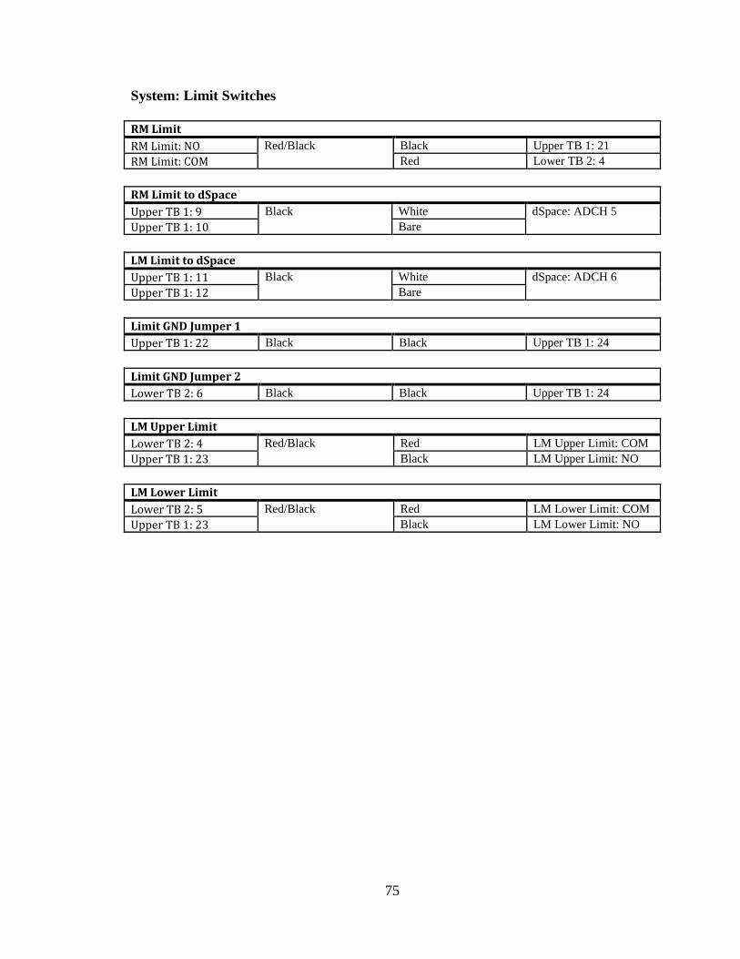
75

System: Limit Switches

RM Limit

RM Limit: NO Red/Black Black Upper TB 1: 21

RM Limit: COM Red Lower TB 2: 4

RM Limit to dSpace

Upper TB 1: 9 Black White dSpace: ADCH 5

Upper TB 1: 10 Bare

LM Limit to dSpace

Upper TB 1: 11 Black White dSpace: ADCH 6

Upper TB 1: 12 Bare

Limit GND Jumper 1

Upper TB 1: 22 Black Black Upper TB 1: 24

Limit GND Jumper 2

Lower TB 2: 6 Black Black Upper TB 1: 24

LM Upper Limit

Lower TB 2: 4 Red/Black Red LM Upper Limit: COM

Upper TB 1: 23 Black LM Upper Limit: NO

LM Lower Limit

Lower TB 2: 5 Red/Black Red LM Lower Limit: COM

Upper TB 1: 23 Black LM Lower Limit: NO

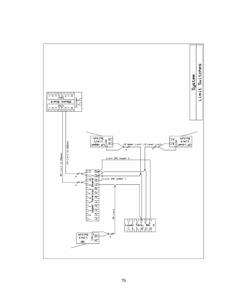
76

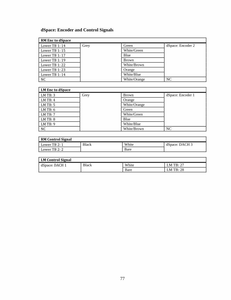
77

dSpace: Encoder and Control Signals

RM Enc to dSpace

Lower TB 1: 14 Grey Green dSpace: Encoder 2

Lower TB 1: 15 White/Green

Lower TB 1: 17 Blue

Lower TB 1: 19 Brown

Lower TB 1: 22 White/Brown

Lower TB 1: 23 Orange

Lower TB 1: 14 White/Blue

NC White/Orange NC

LM Enc to dSpace

LM TB: 3 Grey Brown dSpace: Encoder 1

LM TB: 4 Orange

LM TB: 5 White/Orange

LM TB: 6 Green

LM TB: 7 White/Green

LM TB: 8 Blue

LM TB: 9 White/Blue

NC White/Brown NC

RM Control Signal

Lower TB 2: 1 Black White dSpace: DACH 3

Lower TB 2: 2 Bare

LM Control Signal

dSpace: DACH 1 Black White LM TB: 27

Bare LM TB: 28

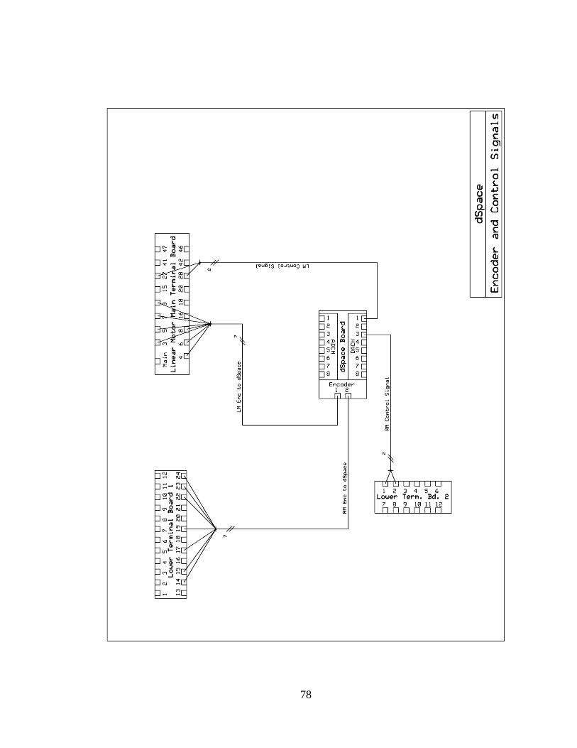
78

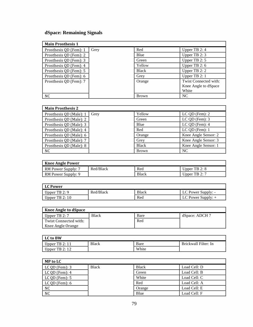
79

dSpace: Remaining Signals

Main Prosthesis 1

Prosthesis QD (Fem): 1 Grey Red Upper TB 2: 4

Prosthesis QD (Fem): 2 Blue Upper TB 2: 3

Prosthesis QD (Fem): 3 Green Upper TB 2: 5

Prosthesis QD (Fem): 4 Yellow Upper TB 2: 6

Prosthesis QD (Fem): 5 Black Upper TB 2: 2

Prosthesis QD (Fem): 6 Grey Upper TB 2: 1

Prosthesis QD (Fem): 7 Orange Twist Connected with:

Knee Angle to dSpace

White

NC Brown NC

Main Prosthesis 2

Prosthesis QD (Male): 1 Grey Yellow LC QD (Fem): 2

Prosthesis QD (Male): 2 Green LC QD (Fem): 3

Prosthesis QD (Male): 3 Blue LC QD (Fem): 4

Prosthesis QD (Male): 4 Red LC QD (Fem): 1

Prosthesis QD (Male): 6 Orange Knee Angle Sensor: 2

Prosthesis QD (Male): 7 Grey Knee Angle Sensor: 3

Prosthesis QD (Male): 8 Black Knee Angle Sensor: 1

NC Brown NC

Knee Angle Power

RM Power Supply: 7 Red/Black Red Upper TB 2: 8

RM Power Supply: 9 Black Upper TB 2: 7

LC Power

Upper TB 2: 9 Red/Black Black LC Power Supply: -

Upper TB 2: 10 Red LC Power Supply: +

Knee Angle to dSpace

Upper TB 2: 7 Black Bare dSpace: ADCH 7

Twist Connected with: Knee Angle Orange

Red

LC to BW

Upper TB 2: 11 Black Bare Brickwall Filter: In

Upper TB 2: 12 White

MP to LC

LC QD (Fem): 3 Black Black Load Cell: D

LC QD (Fem): 4 Green Load Cell: B

LC QD (Fem): 5 White Load Cell: C

LC QD (Fem): 6 Red Load Cell: A

NC Orange Load Cell: E

NC Blue Load Cell: F

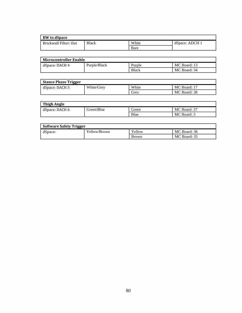
80

BW to dSpace

Brickwall Filter: Out Black White dSpace: ADCH 1

Bare

Microcontroller Enable

dSpace: DACH 4 Purple/Black Purple MC Board: 13

Black MC Board: 34

Stance Phase Trigger

dSpace: DACH 5 White/Grey White MC Board: 17

Grey MC Board: 38

Thigh Angle

dSpace: DACH 6 Green/Blue Green MC Board: 37 Blue MC Board: 3

Software Safety Trigger

dSpace: Yellow/Brown Yellow MC Board: 36 Brown MC Board: 35

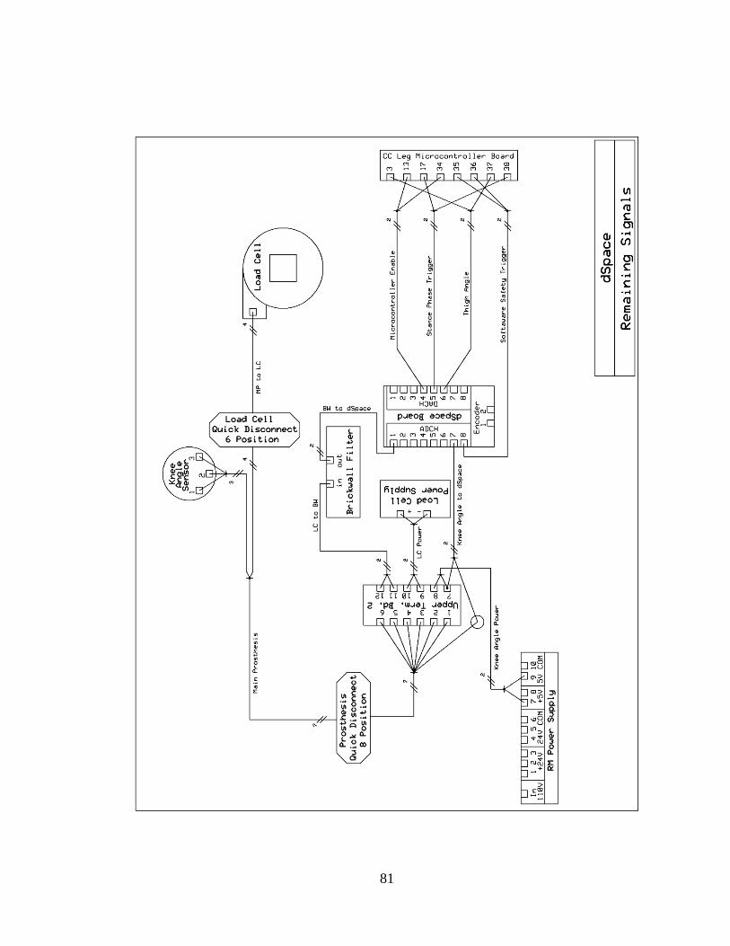
81

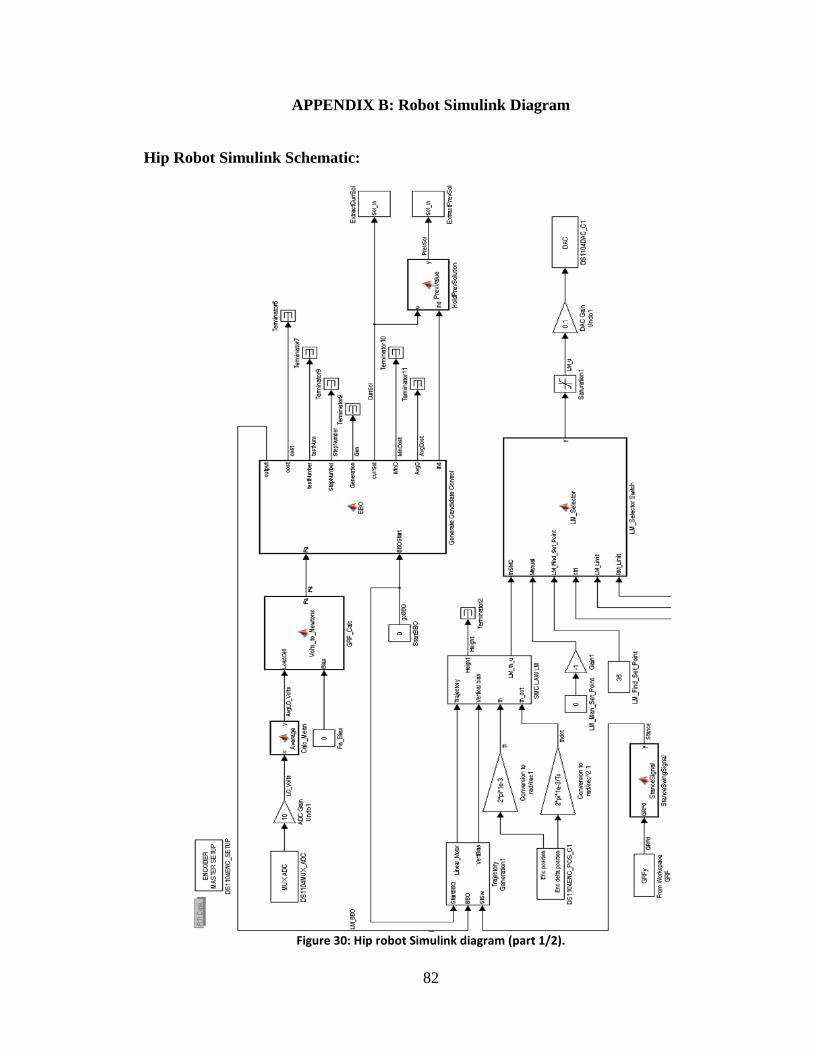
82

APPENDIX B: Robot Simulink Diagram

Hip Robot Simulink Schematic:

Figure 30: Hip robot Simulink diagram (part 1/2).

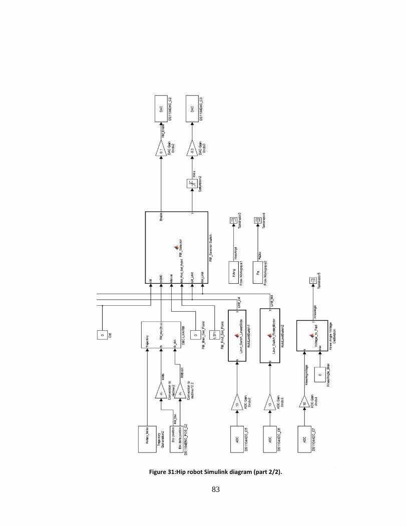
83

Figure 31:Hip robot Simulink diagram (part 2/2).

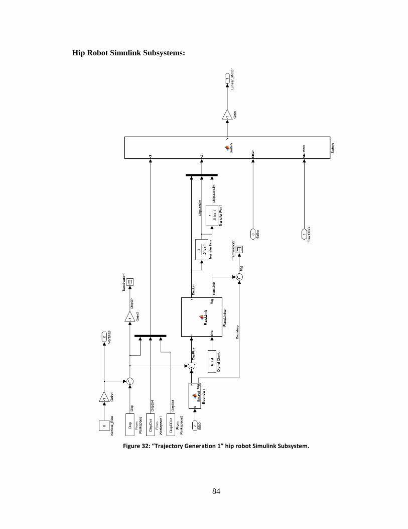
84

Hip Robot Simulink Subsystems:

Figure 32: “Trajectory Generation 1” hip robot Simulink Subsystem.

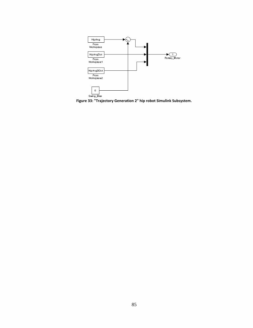
85

Figure 33: "Trajectory Generation 2" hip robot Simulink Subsystem.

86

APPENDIX C: dSpace

Here we document the HR dSpace-HMI. The following are the instruments we

use in dSpace. Following the instruments are screenshots of the actual HR dSpace-HMI.

Instruments

The slider, Figure 15, allows us to adjust a variable in Simulink by moving the

slider. This is especially useful when tuning a controller where slight adjustments are

necessary. We also use the slider to manually adjust the position of the drive-stages.

Figure 34: Slider from dSpace.

The input box, Figure 16, allows us to overwrite the value of a variable by

inputting its new value with the keyboard. We use this to set the initial starting positions

of the drive stages.

Figure 35: Input box from dSpace.

The plotter, Figure 17, is a graphical display of one or more signals over time. For

our purposes we graph the encoder position feedback versus the desired set point so that

we can monitor our controller’s tracking.

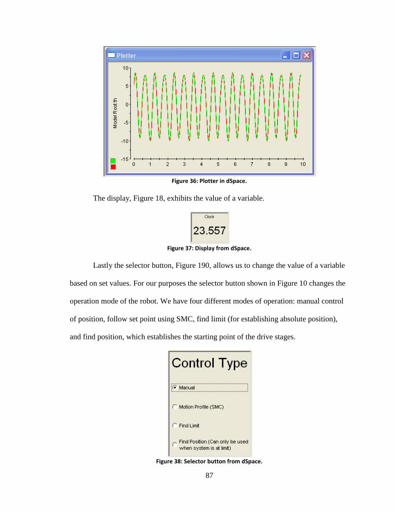
87

Figure 36: Plotter in dSpace.

The display, Figure 18, exhibits the value of a variable.

Figure 37: Display from dSpace.

Lastly the selector button, Figure 190, allows us to change the value of a variable

based on set values. For our purposes the selector button shown in Figure 10 changes the

operation mode of the robot. We have four different modes of operation: manual control

of position, follow set point using SMC, find limit (for establishing absolute position),

and find position, which establishes the starting point of the drive stages.

Figure 38: Selector button from dSpace.

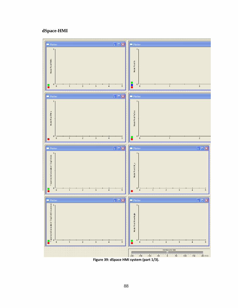
88

dSpace-HMI

Figure 39: dSpace HMI system (part 1/3).

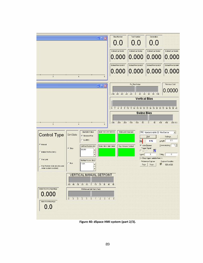
89

Figure 40: dSpace HMI system (part 2/3).

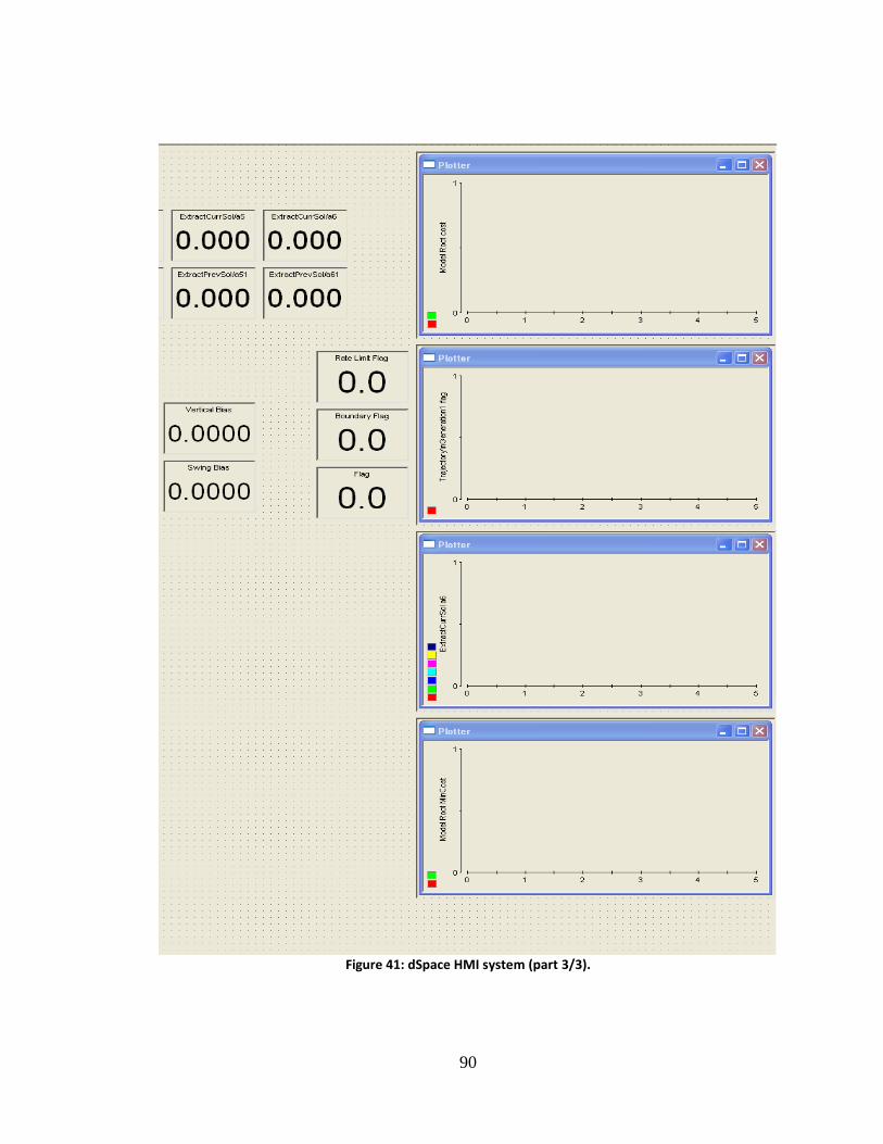
90

Figure 41: dSpace HMI system (part 3/3).