Evolution of magnetic ﬁelds and energetics of ﬂares in ...

Astronomy & Astrophysics manuscript no. all˙ar8210 February 3, 2006(DOI: will be inserted by hand later)

Evolution of magnetic fields and energetics of flaresin active region 8210

Stephane Regnier1,? and Richard C. Canfield2

1 ESA Research and Scientific Support Department, SCI-SH, Keplerlaan 1, 2201 AZ Noordwijk, The [email protected]

2 Montana State University, Physics Dept., 264 EPS Building, Bozeman, MT 59717, USA

Received; Accepted

Abstract. To better understand eruptive events in the solar corona, we combine sequences of multi-wavelength observationsand modelling of the coronal magnetic field of NOAA AR 8210, a highly flare-productive active region. From the photosphereto the corona, the observations give us information about the motion of magnetic elements (photospheric magnetograms), thelocation of flares (e.g., Hα, EUV or soft X-ray brightenings), and the type of events (Hα blueshift events). Assuming thatthe evolution of the coronal magnetic field above an active region can be described by successive equilibria, we follow intime the magnetic changes of the 3D nonlinear force-free (nlff) fields reconstructed from a time series of photospheric vectormagnetograms. We apply this method to AR 8210 observed on May 1, 1998 between 17:00 UT and 21:40 UT. We identifytwo types of horizontal photospheric motions that can drive an eruption: a clockwise rotation of the sunspot, and a fast motionof an emerging polarity. The reconstructed nlff coronal fields give us a scenario of the confined flares observed in AR 8210:the slow sunspot rotation enables the occurence of flare by a reconnection process close to a separatrix surface whereas thefast motion is associated with small-scale reconnections but no detectable flaring activity. We also study the injection rates ofmagnetic energy, Poynting flux and relative magnetic helicity through the photosphere and into the corona. The injection ofmagnetic energy by transverse photospheric motions is found to be correlated with the storage of energy in the corona andthen the release by flaring activity. The magnetic helicity is derived from the magnetic field and the vector potential of the nlffconfiguration is computed in the coronal volume. The magnetic helicity evolution shows that AR 8210 is dominated by themutual helicity between the closed and potential fields and not by the self helicity of the closed field which characterizes thetwist of confined flux bundles. We conclude that for AR 8210 the complex topology is a more important factor than the twist inthe eruption process.

Key words. Sun:magnetic fields, Sun:flares, Sun:corona, Sun:evolution

1. Introduction

The structure of the Sun’s corona is dominated by its mag-netic field. To understand eruptive events (flares, coronal massejections (CMEs) or filament eruptions), we need to know theevolution of the 3D magnetic configuration (geometry and to-pology) of the corona. In this study, we combine observationsof the solar atmosphere at various heights with models of thecoronal magnetic field to determine the sources of flaring activ-ity and the time changes of an active region before and after aflare. We focus our study on a five-hour period which is par-ticularly interesting because (i) it precedes a major flare/CMEevent and (ii) it is well observed with vector magnetograms.

Most flare models (see review by Priest & Forbes 2002; Linet al. 2003) involve magnetic reconnection processes to explainthe rapid conversion of magnetic energy into kinetic energy andthermal energy (hard X-ray sources, soft X-ray flux, brighten-

? Now at St Andrews University, School of Mathematics, NorthHaugh, St Andrews, Fife KY16 9SS, UK

ing in hot EUV lines or in Hα). In the classical CSHKP model(Carmichael 1964; Sturrock 1968; Hirayama 1974; Kopp &Pneuman 1976), the reconnection process occurs at the loca-tion of an X point in 2D, or at the location of a null point or aseparator field line in 3D. In 3D topology (see Priest & Forbes2000), the reconnection processes involved in flares do not oc-cur only in the vicinity of a null point but can also be associatedwith other topological elements (e.g., fan surfaces, spine fieldlines). The study of the topology of coronal magnetic fieldsshould help us to answer important questions for the energet-ics of flares, including (i) how is magnetic energy stored be-fore the eruption? (ii) is the stored magnetic energy enough topower a flare or a CME? Question (i) can be tackled by follow-ing the time evolution of the magnetic energy injected throughthe photosphere, and the free magnetic energy available in thecorona. To answer question (ii), we need to understand the tem-poral and spatial relationship between observed brighteningsand magnetic field changes in the corona.

2 Regnier & Canfield: AR 8210 evolution

Table 1. Photospheric, chromospheric and coronal observations of AR 8210 on May 1, 1998. ∆x is the pixel size, ∆t is the time between twoconsecutive observations.

Instrument Wavelength Obs. Time ∆x ∆t

SOHO/MDI Ni I at 676.8 nm 17:00–23:00 1′′.98 1 minMSO/IVM FeI at 630.25 nm 17:07–21:40 1′′.1 3 minNSO/BBSO Hα at 656.3 nm 17:00–21:08 1′′ 1 min

MSO/MCCD ” 17:00–22:00 2′′.4 15 sSOHO/EIT Fe XII at 19.5 nm 17:00–23:00 2′′.46 15 min

Yohkoh/SXT Soft X-rays 17:16–22:16 4′′.9 & 9′′.8 ∼ 8min

The injection of magnetic energy into the corona throughthe photosphere is considered to be associated with the hori-zontal displacement of magnetic features on the photosphere:emergence (Schmieder et al. 1997; Ishii et al. 1998; Kusanoet al. 2002; Nindos & Zhang 2002) and cancellation (Livi et al.1989; Fletcher et al. 2001) of magnetic flux, rotation of sun-spots (Kucera 1982; Lin & Chen 1989; Nightingale et al. 2002),and moving magnetic features (Zhang & Wang 2001; Moonet al. 2002). The velocity fields can be detrmined using thewhite light images (Nightingale et al. 2002) or by estimatingthe small displacements from a Local Correlation Tracking(LCT) technique (November & Simon 1988). Recently sev-eral more powerful techniques have been developed to retrievethe full photospheric velocity field from vector magnetograms(Welsch et al. 2004; Longcope 2004; Georgoulis & LaBonte2005).

In our study, the coronal magnetic field is assumed to bein a force-free equilibrium state at the time of observation.Therefore if the photospheric distribution of vertical electriccurrent density is known in addition to the vertical magneticfield (Sakurai 1982), the nonlinear force-free field (nlff) can beextrapolated in the corona (e..g., Mikic & McClymont 1994;Amari et al. 1997; Wheatland et al. 2000; Yan & Sakurai2000; Wiegelmann 2004). Inside nlff magnetic configurations,a more realistic distribution of twist and shear can be con-sidered in comparison to other assumptions commonly used toextrapolate the coronal magnetic field (potential, linear force-free fields). These nlff extrapolation methods were applied tosolar active regions using one snapshot of the magnetic field(e.g., Yan & Wang 1995; Regnier et al. 2002; Bleybel et al.2002; Regnier & Amari 2004). Here we propose to study thetime evolution of an active region considering that it can bedescribed by succesive nonlinear force-free equilibria. This as-sumption is justified by considering that the evolution of theactive region is sufficiently slow which means that the pho-tospheric velocities of the footpoints are small compared tocharacteristic speeds in the corona, such as the Alfven velocity(Antiochos 1987).

Using the above methods to estimate the velocity fields onthe photosphere and the 3D coronal magnetic field, we can es-timate the rate of magnetic energy injected into the corona byphotospheric motions and where this energy is deposited orreleased in the corona. We can also derive the magnetic heli-city and its evolution to understand the effects of reconnectionon the connectivity of field lines. In this work, we have se-

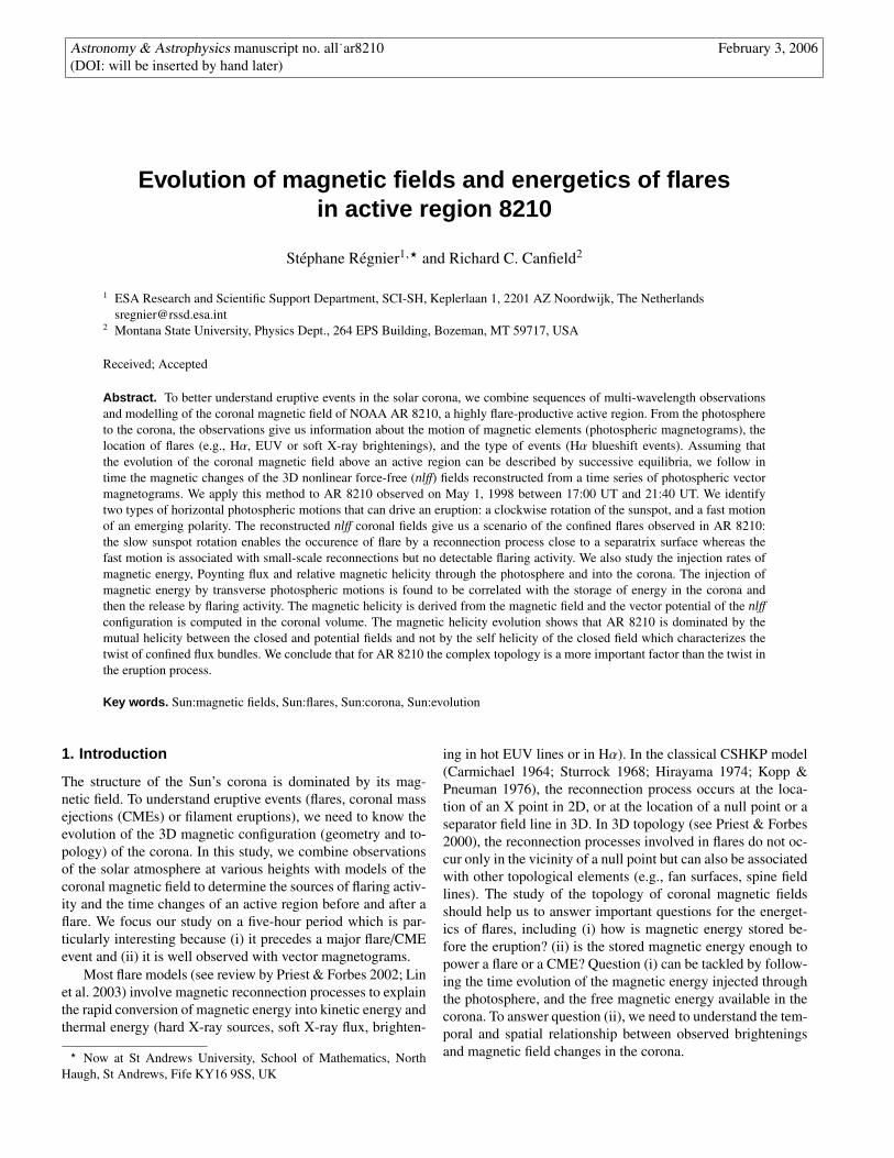
lected the active region 8210 (AR 8210) observed on May 1,1998 between 17:00 UT and 21:40 UT for which we have agood set of data covering the photosphere, the chromosphereand the corona as well as a high-cadence vector magnetic fieldobservations of good quality. AR 8210 is a well studied act-ive region for its flaring activity on May 1st and May 2nd(Thompson et al. 2000; Warmuth et al. 2000; Pohjolainen et al.2001; Sterling & Moore 2001a,b; Xia et al. 2001; Sterling et al.2001; Wang et al. 2002). We focus our attention on the timeperiod shown in Fig. 1 by the evolution of the X-ray flux. Wefirst give an overview of the AR 8210 data (see Section 2) weuse to analyse the precursors or signatures of flaring activity(Section 3): X-ray flux, Hα blueshift events (BSEs), photo-spheric velocity fields. In Section 4, we describe how to de-termine and analyse the 3D magnetic field of AR 8210. Wethen give a scenario of the magnetic field evolution during theflaring period (Section 5). The magnetic energy and helicitybudgets are derived in Sections 6 and 7. In Section 8, we dis-cuss the implications of those processes for flaring activity andsolar eruptions.

Fig. 1. X-ray flux measured by GOES-8 in the wavelength range 0.05–0.4 nm. Gray areas are the flaring periods. The rise (resp. decay) phaseof flares are the dark (resp. light) gray areas as defined in Section 3.1.

Regnier & Canfield: AR 8210 evolution 3

2. Data

In Table 1, we summarize the observations on May 1, 1998we are using in this study. Between 17:00 UT and 23:00 UT,we have photospheric line-of-sight and vector magnetograms,chromospheric images and spectra, and coronal images. Thosedata guide the analysis presented in later sections.

2.1. Photospheric Magnetic Field

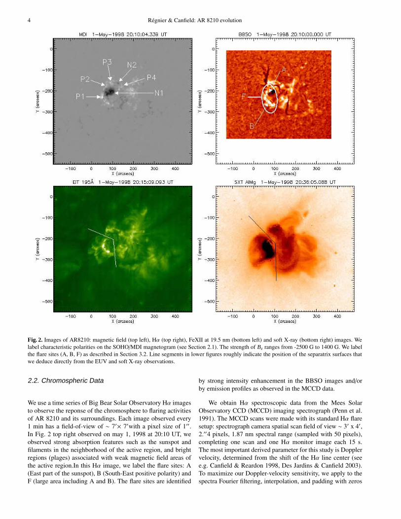
SOHO/MDI (Michelson Doppler Imager, Scherrer et al. 1995)measures the line-of-sight magnetic field strength deducedfrom the Zeeman splitting of the Ni I 676.8 nm line. Duringthe period of observation, we have 1 min cadence full-discmagnetograms which allow us to study the dynamics of pho-tospheric magnetic features. The measurement uncertainty is∼ 20 G. In Fig. 2 top left, we have the distribution of thelongitudinal magnetic field at 20:10 UT in a field-of-view of600”×600”. Basically AR 8210 is a sunspot complex of neg-ative polarity (polarity N1) surrounding by positive polarities(P1–4). AR 8210 also includes parasitic polarities such as N2,which is a new emerged and moving negative polarity.

IVM at MSO (Imaging Vector Magnetograph/Mees SolarObservatory, Mickey et al. 1996) is a vector magnetographmeasuring the full Stokes profiles of the Fe I 630.25 nm line.The four Stokes parameters, I = (I,Q,U,V), are measuredinside a field-of-view of 256x256 pixels with a pixel size of1.1′′square. The vector magnetograms are built with a seriesof 30 polarisation images obtained over 3 min (Mickey et al.1996). To increase the signal-to-noise ratio and to suppress theeffects of photospheric oscillations, we average the Stokes pro-files over 15 min. In the reduction process, we take into accountthe cross-talk between the I and V profiles as well as scatteredlight using daily off-limb measurements. A detailed reductionscheme is given by LaBonte et al. (1999). To infer the mag-netic field, the inversion code follows the radiative transfer ofline profiles as in Landolfi & Degl’innocenti (1982) based onUnno (1956) equations and including magneto-optical effects.We then obtain the magnetic field: Blos along the line-of-sight,Btrans and χ the strength and the azimuthal angle of the trans-verse components (in the plane perpendicular to the line-of-sight). We perform the transformation into the disc-center he-liographic system of coordinates and resolve the 180o ambi-guity existing on the transverse field following Canfield et al.(1993). The resulting magnetic field in a Cartesian frame is(Bx, By, Bz).

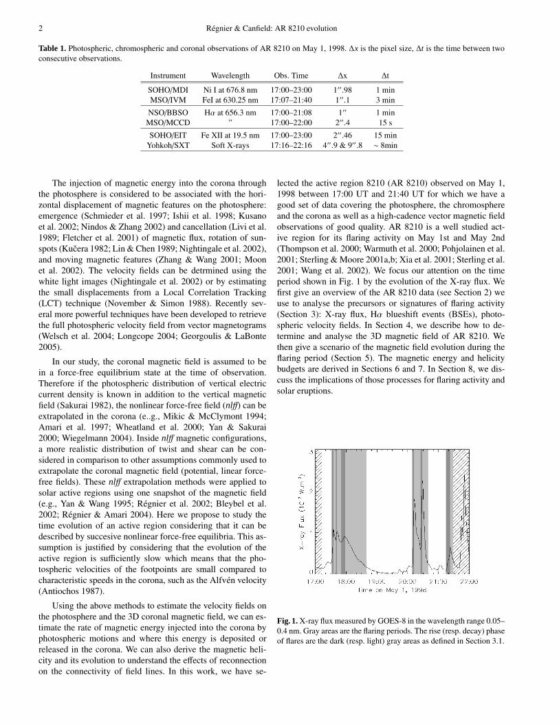
We have performed an analysis of the noise level for thevertical and the transverse components of the magnetic fieldon each of the 15 averaged magnetograms. We proceed as fol-lows: for the vertical magnetic field we plot the distributionwhich can be fitted with a gaussian profile, for the transversefield we fit the distribution with a χ2 distribution. In both cases,the estimated error is defined as the 3σ value associated withthe width (σ) of the fitted distribution (see Leka & Skumanich1999, Leka 1999). In Fig. 3, we plot the time evolution of thephotospheric unsigned magnetic flux as well as the associatederrors (from the 3σ errors on the Bz component) to show thequality of the data. The estimated formal errors on Bz range

Fig. 3. Unsigned magnetic flux for the IVM time series and the asso-ciated errors (unit of 1022 G.cm2). Gray areas are the flaring periodsas defined in Fig. 1.

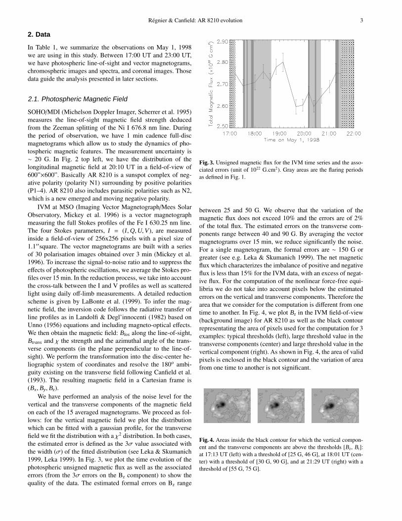
between 25 and 50 G. We observe that the variation of themagnetic flux does not exceed 10% and the errors are of 2%of the total flux. The estimated errors on the transverse com-ponents range between 40 and 90 G. By averaging the vectormagnetograms over 15 min, we reduce significantly the noise.For a single magnetogram, the formal errors are ∼ 150 G orgreater (see e.g. Leka & Skumanich 1999). The net magneticflux which characterizes the imbalance of positive and negativeflux is less than 15% for the IVM data, with an excess of negat-ive flux. For the computation of the nonlinear force-free equi-libria we do not take into account pixels below the estimatederrors on the vertical and transverse components. Therefore thearea that we consider for the computation is different from onetime to another. In Fig. 4, we plot Bz in the IVM field-of-view(background image) for AR 8210 as well as the black contourrepresentating the area of pixels used for the computation for 3examples: typical thresholds (left), large threshold value in thetransverse components (center) and large threshold value in thevertical component (right). As shown in Fig. 4, the area of validpixels is enclosed in the black contour and the variation of areafrom one time to another is not significant.

Fig. 4. Areas inside the black contour for which the vertical compon-ent and the transverse components are above the thresholds [Bz, Bt]:at 17:13 UT (left) with a threshold of [25 G, 46 G], at 18:01 UT (cen-ter) with a threshold of [30 G, 90 G], and at 21:29 UT (right) with athreshold of [55 G, 75 G].


Fig. 2. Images of AR8210: magnetic field (top left), Hα (top right), FeXII at 19.5 nm (bottom left) and soft X-ray (bottom right) images. Welabel characteristic polarities on the SOHO/MDI magnetogram (see Section 2.1). The strength of Bz ranges from -2500 G to 1400 G. We labelthe flare sites (A, B, F) as described in Section 3.2. Line segments in lower figures roughly indicate the position of the separatrix surfaces thatwe deduce directly from the EUV and soft X-ray observations.

2.2. Chromospheric Data

We use a time series of Big Bear Solar Observatory Hα imagesto observe the reponse of the chromosphere to flaring activitiesof AR 8210 and its surroundings. Each image observed every1 min has a field-of-view of ∼ 7′× 7′with a pixel size of 1′′.In Fig. 2 top right observed on may 1, 1998 at 20:10 UT, weobserved strong absorption features such as the sunspot andfilaments in the neighborhood of the active region, and brightregions (plages) associated with weak magnetic field areas ofthe active region.In this Hα image, we label the flare sites: A(East part of the sunspot), B (South-East positive polarity) andF (large area including A and B). The flare sites are identified

by strong intensity enhancement in the BBSO images and/orby emission profiles as observed in the MCCD data.

We obtain Hα spectroscopic data from the Mees SolarObservatory CCD (MCCD) imaging spectrograph (Penn et al.1991). The MCCD scans were made with its standard Hα flaresetup: spectrograph camera spatial scan field of view ∼ 3′ x 4′,2.′′4 pixels, 1.87 nm spectral range (sampled with 50 pixels),completing one scan and one Hα monitor image each 15 s.The most important derived parameter for this study is Dopplervelocity, determined from the shift of the Hα line center (seee.g. Canfield & Reardon 1998, Des Jardins & Canfield 2003).To maximize our Doppler-velocity sensitivity, we apply to thespectra Fourier filtering, interpolation, and padding with zeros


A

B

F

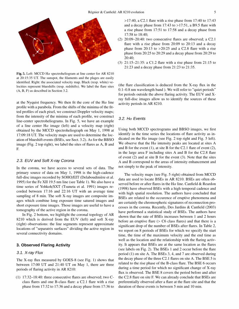
Fig. 5. Left: MCCD Hα spectroheliogram at line center for AR 8210at 20:15:35 UT. The sunspot, the filaments and the plages are easilyidentified. Right: the associated velocity map. Black (resp. white) ve-locities represent blueshifts (resp. redshifts). We label the flare sites(A, B, F) as described in Section 3.2.

at the Nyquist frequency. We then fit the core of the Hα lineprofile with a parabola. From the shifts of the minima of the fit-ted profiles of each pixel, we construct Doppler velocity maps;from the intensity of the minima of each profile, we constructline-center spectroheliograms. In Fig. 5, we have an exampleof a line center Hα image (left) and a velocity map (right)obtained by the MCCD spectroheliograph on May 1, 1998 at17:09:18 UT. The velocity maps are used to determine the loc-ation of blueshift events (BSEs, see Sect. 3.2). As for the BBSOimage (Fig. 2 top right), we label the sites of flares as A, B andF.

2.3. EUV and Soft X-ray Corona

In the corona, we have access to several sets of data. Theprimary source of data on May 1, 1998 is the high-cadencefull-disc images recorded by SOHO/EIT (Delaboudiniere et al.1995) for the Fe XII 19.5 nm line (see Table 1). We also have atime series of Yohkoh/SXT (Tsuneta et al. 1991) images re-corded between 17:16 and 22:16 UT with an average timesampling of 8 min. The soft X-ray images are composite im-ages which combine long exposure time satured images andshort exposure time images. Those images are useful to have atomography of the active region in the corona.

In Fig. 2 bottom, we highlight the coronal topology of AR8210 which is derived from the EUV (left) and soft X-ray(right) observations: the line segments represent approximatelocations of ”separatrix surfaces” dividing the active region inseveral connectivity domains.

3. Observed Flaring Activity

3.1. X-ray Flux

The X-ray flux measured by GOES-8 (see Fig. 1) shows thatbetween 17:00 UT and 21:40 UT on May 1, there are threeperiods of flaring activity in AR 8210:

(1) 17:32–18:40: three consecutive flares are observed; two C-class flares and one B-class flare: a C2.1 flare with a risephase from 17:32 to 17:36 and a decay phase from 17:36 to

>17:40, a C2.1 flare with a rise phase from 17:40 to 17:43and a decay phase from 17:43 to >17:51, a B9.5 flare witha rise phase from 17:51 to 17:58 and a decay phase from17:58 to 18:40;

(2) 20:09–20:40: two consecutive flares are observed; a C2.1flare with a rise phase from 20:09 to 20:13 and a decayphase from 20:13 to >20:25 and a C2.8 flare with a risephase from 20:25 to 20:29 and a decay phase from 20:29 to20:40;

(3) 21:15–21:35: a C1.2 flare with a rise phase from 21:15 to21:23 and a decay phase from 21:23 to 21:35.

(the flare classification is deduced from the X-ray flux in the0.1–0.8 nm wavelength band ). We will refer to ”quiet periods”for periods outside the above flaring activity. The EUV and X-ray full-disc images allow us to identify the sources of theseactivity periods in AR 8210.

3.2. Hα Events

Using both MCCD spectrograms and BBSO images, we firstidentify in the time series the locations of flare activity as in-dicated on the Hα image (see Fig. 2 top right and Fig. 5 left).We observe that the Hα intensity peaks are located at sites Aand B for the event (1), at site B for the C2.1 flare of event (2),in the large area F including sites A and B for the C2.8 flareof event (2) and at site B for the event (3). Note that the sitesA and B correspond to the areas of intensity enhancement andnot simply to the peak of intensity.

The velocity maps (see Fig. 5 right) obtained from MCCDdata are used to locate BSEs in AR 8210. BSEs are often ob-served before or after flares in the Hα line. Canfield & Reardon(1998) have observed BSEs with a high temporal cadence andwith high spatial resolution. The authors have concluded thatBSEs are related to the occurence of eruptive phenomena andare certainly the chromospheric signatures of reconnection pro-cesses in the corona. Recently, Des Jardins & Canfield (2003)have performed a statistical study of BSEs. The authors haveshown that the rate of BSEs increases between 1 and 2 hoursbefore an eruptive flare (> C6 class flares) and that there is asignificant drop of the number of BSEs after flares. In Table 2,we report on 8 periods of BSEs for which we specify the starttime, the time of the maximum velocity and the end time aswell as the location and the relationship with the flaring activ-ity. It appears that BSEs are at the same location as the flares(see labels on Fig. 2). The BSEs 1 and 2 occur before the flareperiod (1) on site A. The BSEs 3, 4, and 7 are observed duringthe decay phase of the three C2.1 flares on site A. The BSE 5 isrelated to the rise phase of the B-class flare. The BSE 6 occursduring a time period for which no significant change of X-rayflux is observed. The BSE 8 covers the period before and afterthe C2.8 flare on site F. We can already conclude that BSEs arepreferentially observed after a flare at the flare site and that theduration of these events is between 5 min and 10 min.


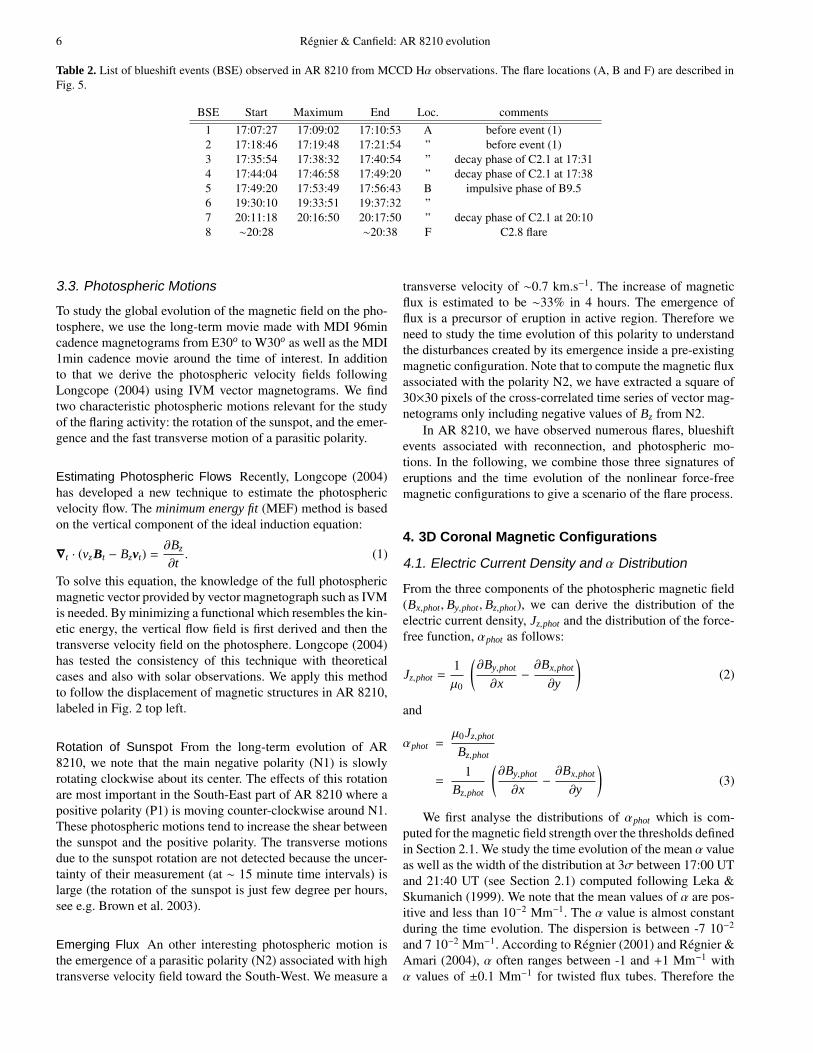
Table 2. List of blueshift events (BSE) observed in AR 8210 from MCCD Hα observations. The flare locations (A, B and F) are described inFig. 5.

BSE Start Maximum End Loc. comments1 17:07:27 17:09:02 17:10:53 A before event (1)2 17:18:46 17:19:48 17:21:54 ” before event (1)3 17:35:54 17:38:32 17:40:54 ” decay phase of C2.1 at 17:314 17:44:04 17:46:58 17:49:20 ” decay phase of C2.1 at 17:385 17:49:20 17:53:49 17:56:43 B impulsive phase of B9.56 19:30:10 19:33:51 19:37:32 ”7 20:11:18 20:16:50 20:17:50 ” decay phase of C2.1 at 20:108 ∼20:28 ∼20:38 F C2.8 flare

3.3. Photospheric Motions

To study the global evolution of the magnetic field on the pho-tosphere, we use the long-term movie made with MDI 96mincadence magnetograms from E30o to W30o as well as the MDI1min cadence movie around the time of interest. In additionto that we derive the photospheric velocity fields followingLongcope (2004) using IVM vector magnetograms. We findtwo characteristic photospheric motions relevant for the studyof the flaring activity: the rotation of the sunspot, and the emer-gence and the fast transverse motion of a parasitic polarity.

Estimating Photospheric Flows Recently, Longcope (2004)has developed a new technique to estimate the photosphericvelocity flow. The minimum energy fit (MEF) method is basedon the vertical component of the ideal induction equation:

∇t · (vzBt − Bzvt) =∂Bz

∂t. (1)

To solve this equation, the knowledge of the full photosphericmagnetic vector provided by vector magnetograph such as IVMis needed. By minimizing a functional which resembles the kin-etic energy, the vertical flow field is first derived and then thetransverse velocity field on the photosphere. Longcope (2004)has tested the consistency of this technique with theoreticalcases and also with solar observations. We apply this methodto follow the displacement of magnetic structures in AR 8210,labeled in Fig. 2 top left.

Rotation of Sunspot From the long-term evolution of AR8210, we note that the main negative polarity (N1) is slowlyrotating clockwise about its center. The effects of this rotationare most important in the South-East part of AR 8210 where apositive polarity (P1) is moving counter-clockwise around N1.These photospheric motions tend to increase the shear betweenthe sunspot and the positive polarity. The transverse motionsdue to the sunspot rotation are not detected because the uncer-tainty of their measurement (at ∼ 15 minute time intervals) islarge (the rotation of the sunspot is just few degree per hours,see e.g. Brown et al. 2003).

Emerging Flux An other interesting photospheric motion isthe emergence of a parasitic polarity (N2) associated with hightransverse velocity field toward the South-West. We measure a

transverse velocity of ∼0.7 km.s−1. The increase of magneticflux is estimated to be ∼33% in 4 hours. The emergence offlux is a precursor of eruption in active region. Therefore weneed to study the time evolution of this polarity to understandthe disturbances created by its emergence inside a pre-existingmagnetic configuration. Note that to compute the magnetic fluxassociated with the polarity N2, we have extracted a square of30×30 pixels of the cross-correlated time series of vector mag-netograms only including negative values of Bz from N2.

In AR 8210, we have observed numerous flares, blueshiftevents associated with reconnection, and photospheric mo-tions. In the following, we combine those three signatures oferuptions and the time evolution of the nonlinear force-freemagnetic configurations to give a scenario of the flare process.

4. 3D Coronal Magnetic Configurations

4.1. Electric Current Density and α Distribution

From the three components of the photospheric magnetic field(Bx,phot, By,phot, Bz,phot), we can derive the distribution of theelectric current density, Jz,phot and the distribution of the force-free function, αphot as follows:

Jz,phot =1µ0

(

∂By,phot

∂x−∂Bx,phot

∂y

)

(2)

and

αphot =µ0Jz,phot

Bz,phot

=1

Bz,phot

(

∂By,phot

∂x−∂Bx,phot

∂y

)

(3)

We first analyse the distributions of αphot which is com-puted for the magnetic field strength over the thresholds definedin Section 2.1. We study the time evolution of the mean α valueas well as the width of the distribution at 3σ between 17:00 UTand 21:40 UT (see Section 2.1) computed following Leka &Skumanich (1999). We note that the mean values of α are pos-itive and less than 10−2 Mm−1. The α value is almost constantduring the time evolution. The dispersion is between -7 10−2

and 7 10−2 Mm−1. According to Regnier (2001) and Regnier &Amari (2004), α often ranges between -1 and +1 Mm−1 withα values of ±0.1 Mm−1 for twisted flux tubes. Therefore the


α value and its dispersion indicate that there is only a smallamount of twist in AR 8210.

In order to describe the coronal field as a nonlinear force-free equilibrium, there are several requirements on the prop-erties of the current density distribution, Jz,phot. The electriccurrent should be balanced: the total electric current should bezero. The positive currents from one polarity should be equal tothe negative currents in the opposite polarity. These propertiescan be written as follows:∫

Σ+

Jz,phot dS =∫

Σ−

Jz,phot dS , (4)

and∫

Σ+

|J±z,phot | dS =∫

Σ−

|J∓z,phot | dS , (5)

and consequently,∫

Σ±

Jz,phot dS = 0 (6)

where Σ+ (resp. Σ−) is where Bz,phot > 0 (resp. Bz,phot < 0) andJ±z,phot is only considered where Jz,phot is positive or negativerespectively.

As an example, we study the distributions for the IVM vec-tor magnetogram at 17:13 UT. The thresholds on the magneticfield components are 25 G for Bz and 46 G for Bt. The ratio ofthe area of strong field region to the area of weak field regionis about 1.2. The electric current imbalance (from Eqn. (4)) is8% and from Eqn. (5) the electric current imbalance is 30%.

The imbalance of electric current is plausibly due to the factthat the current in the strong-field regions is detected becausethe observed fields there exceed the threshold required for Jz

calculations while that in weak-field regions is not detected.Note that the imbalance is negative, as one would expect, sinceJz is mostly negative in the sunspot N1 where the field strengthis high and then Jz well estimated.

4.2. nlff Reconstruction

To determine the structure of the coronal field we use thenonlinear force-free approximation based on a vector poten-tial Grad-Rubin (1958) method by using the XTRAPOL code(Amari et al. 1997, 1999). The nlff field in the corona is thengoverned by the following equations:

∇ ∧ B = αB, (7)

B · ∇α = 0, (8)

∇ · B = 0, (9)

where B is the magnetic field vector in the domain Ω abovethe photosphere, δΩ, and α is a function of space defined as theratio of the vertical current density, Jz and the vertical magneticfield component, Bz (see Eqn. (3)). From Eqn. (8), α is constantalong a field line. In terms of the magnetic field B, the Grad-Rubin iterative scheme can be written as follows:

B(n) · ∇α(n) = 0 in Ω, (10)

α(n)|δΩ± = h, (11)

where δΩ± is defined as the domain on the photosphere forwhich Bz is positive (+) or negative (−) and,

∇ ∧ B(n+1) = α(n)B(n) in Ω, (12)

∇ · B(n+1) = 0 in Ω, (13)

B(n+1)z |δΩ = g, (14)

lim|r|→∞

|B| = 0. (15)

The boundary conditions on the photosphere are given by thedistribution, g of Bz on δΩ (see Eqn. (14)) and by the distribu-tion h of α on δΩ for a given polarity (see Eqn. (11)). We alsoimpose that

Bn = 0 on Σ − δΩ (16)

where Σ is the surface of the computational box, n refers to thenormal component to the surface. These conditions mean thatno field line can enter or leave to computational box, or in otherwords that the studied active region is magnetically isolated.

Practically, the boundary conditions on the photosphereare: the observed vertical component of the magnetic field,Bz,phot in the disc-center heliographic system of coordinates al-lowing the computation in cartesian coordinates, and the αphot

distribution given by Eqn. (3) in a chosen polarity (we havechosen the negative polarity which represents the sunspot N1of the active region). In order to ensure that the entire activeregion is included in the field-of-view, we have created com-posite vector magnetograms by combining IVM magnetograms(strong-field regions) and MDI magnetograms (surroundingweak-field regions). We then compute the nonlinear force-freefield for the time series of composite magnetograms using across-correlation technique between each magnetogram and anon-uniform grid which reduces the computational time. Thoseproperties insure that we reconstruct the same volume of thecorona. Therefore we can study the time evolution of relevantquantities as the magnetic energy or the relative magnetic heli-city.

4.3. Basic Topology

An interesting property of a magnetic configuration is givenby its skeleton. The skeleton (Priest & Forbes 2000) corres-ponds to all topological elements inside a 3D magnetic fieldincluding null points, spine field lines, separatrix surfaces andseparators. To analyse the evolution of AR 8210, we determ-ine various topological elements. First we find the null pointson the photosphere by determining where the magnetic fieldvanishes and corresponds to a local minima and for which thetransverse components vanish. Around the null point, the mag-netic field has three eigenvalues, λi (i = 1, 2, 3), that sum tozero to satisfy Eqn. (9). An eigenvector is associated with eacheigenvalue (not necessarily three perpendicular vectors). If oneeigenvalue is positive (resp. negative) and the two others are


negative (resp. positive), the spine is the isolated field line dir-ected away from (resp. toward) the null and the separatrix sur-face consists of field lines radiating toward (resp. away from)the null. The separatrix surfaces give us the definition of thedifferent connectivity domains that comprise AR 8210.

NN1

PN1

PN2 PN3

NN2

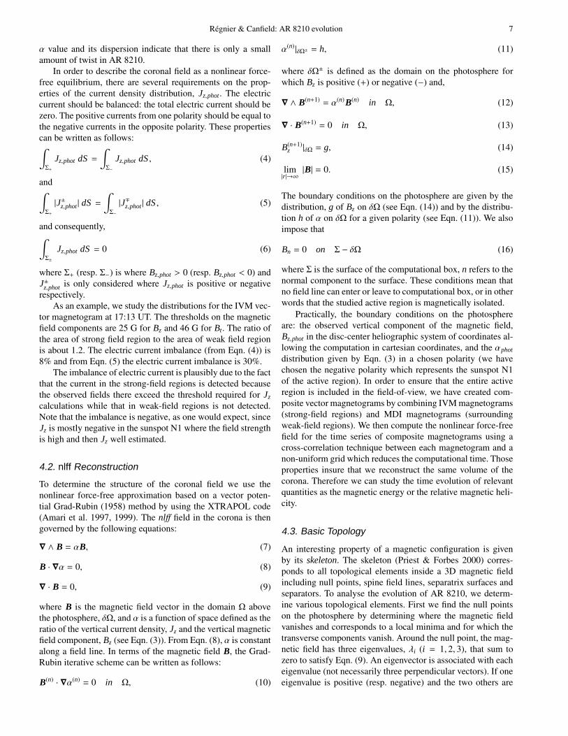
Fig. 6. Basic topological elements for AR 8210 at 17:13 UT. Red(resp. blue) triangles are positive (resp. negative) null points. Spinefield lines are thick white lines and separatrix surfaces (or fan sur-faces) are defined by two green vectors. Only the projection on thephotospheric plane is shown. The characteristic null points are labelledPN1–3 and NN1.

As shown in Fig. 6, AR 8210 exhibits a complex topologywith numerous photospheric null points (triangles) and separat-rix surfaces represented by the direction of the fan surfaces(green lines) and the spine (thick white lines). We only plotthe topological elements inside a reduced field of view. We ob-tain 49 null points in the entire field of view: 26 negative nullsand 23 positive nulls. We focus our study on four nulls: PN1-3and NN1 (PN: positive null, NN: negative null). The null pointsPN1–3 and their associated separatrix surface will be investig-ated in the next section. NN1 has a spine field line connectedwith surrounding negative polarities. The separatrix surface isin the same direction as the South separatrix surface shown onEUV and soft X-ray images (Fig. 2 bottom). The topology doesnot change dramatically during the evolution of AR 8210 (dur-ing the studied time period).

5. Flares, Photospheric Motions and MagneticReconnection

5.1. 3D Magnetic Evolution Associated withPrecursors

We now analyse the coronal magnetic changes during this timeperiod for the emerging, moving magnetic feature, and therotating sunspot (see Section 3.3). We describe small recon-nection processes associated with photospheric motions. By”small” reconnections we mean reconnection processes whichdo not modify the configuration of the entire active region, butfor which the connectivity of field lines is modified locally.

5.1.1. Emerging Flux

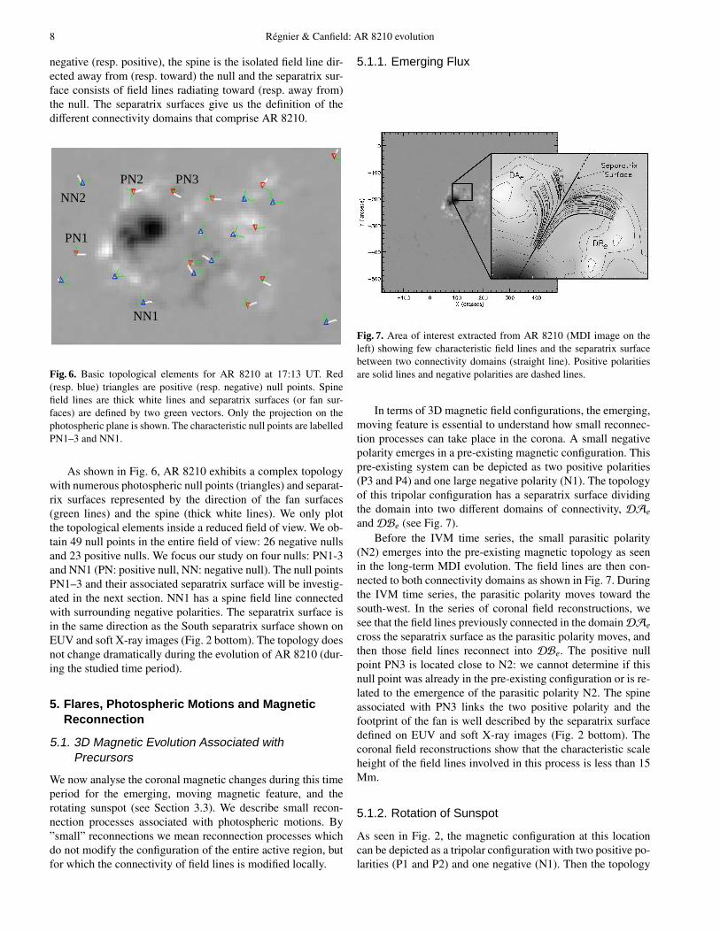
Fig. 7. Area of interest extracted from AR 8210 (MDI image on theleft) showing few characteristic field lines and the separatrix surfacebetween two connectivity domains (straight line). Positive polaritiesare solid lines and negative polarities are dashed lines.

In terms of 3D magnetic field configurations, the emerging,moving feature is essential to understand how small reconnec-tion processes can take place in the corona. A small negativepolarity emerges in a pre-existing magnetic configuration. Thispre-existing system can be depicted as two positive polarities(P3 and P4) and one large negative polarity (N1). The topologyof this tripolar configuration has a separatrix surface dividingthe domain into two different domains of connectivity, DAe

and DBe (see Fig. 7).Before the IVM time series, the small parasitic polarity

(N2) emerges into the pre-existing magnetic topology as seenin the long-term MDI evolution. The field lines are then con-nected to both connectivity domains as shown in Fig. 7. Duringthe IVM time series, the parasitic polarity moves toward thesouth-west. In the series of coronal field reconstructions, wesee that the field lines previously connected in the domainDAe

cross the separatrix surface as the parasitic polarity moves, andthen those field lines reconnect into DBe. The positive nullpoint PN3 is located close to N2: we cannot determine if thisnull point was already in the pre-existing configuration or is re-lated to the emergence of the parasitic polarity N2. The spineassociated with PN3 links the two positive polarity and thefootprint of the fan is well described by the separatrix surfacedefined on EUV and soft X-ray images (Fig. 2 bottom). Thecoronal field reconstructions show that the characteristic scaleheight of the field lines involved in this process is less than 15Mm.

5.1.2. Rotation of Sunspot

As seen in Fig. 2, the magnetic configuration at this locationcan be depicted as a tripolar configuration with two positive po-larities (P1 and P2) and one negative (N1). Then the topology


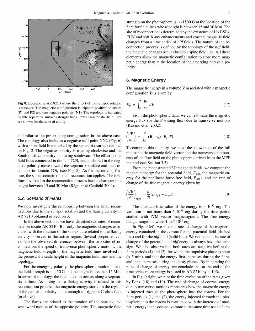
Fig. 8. Location in AR 8210 where the effect of the sunspot rotationis stronger. The magnetic configuration is tripolar: positive polarities(P1 and P2) and one negative polarity (N1). The topology is indicatedby thte separatrix surface (straight line). Few characteristic field linesare shown for the sake of clarity.

is similar to the pre-existing configuration in the above case.The topology also includes a negative null point NN2 (Fig. 6)with a spine field line marked by the separatrix surface definedon Fig. 2. The negative polarity is rotating clockwise and theSouth positive polarity is moving southward. The effect is thatfield lines connected in domain DAr and anchored in the neg-ative polarity move toward the separatrix surface and then re-connect in domain DBr (see Fig. 8). As for the moving fea-ture, the same scenario of small reconnection applies. The fieldlines involved in the reconnection process have a characteristicheight between 15 and 30 Mm (Regnier & Canfield 2004).

5.2. Scenario of Flares

We now investigate the relationship between the small recon-nections due to the sunspot rotation and the flaring activity inAR 8210 obtained in Section 3.

In the above sections, we have identified two sites of recon-nection inside AR 8210. But only the magnetic changes asso-ciated with the rotation of the sunspot are related to the flaringactivity observed in the active region. Several properties canexplain the observed differences between the two sites of re-connection: the speed of transverse photospheric motions, themagnetic field strength of the magnetic field lines involved inthe process, the scale height of the magnetic field lines and thetopology.

For the emerging polarity, the photospheric motion is fast,the field strength is ∼ -450 G and the height is less than 15 Mm.In terms of topology, the reconnection occurs along a separat-rix surface. Assuming that a flaring activity is related to thisreconnection process, the magnetic energy stored in the regionof the parasitic polarity is not enough to trigger a C-class flare(or above)

The flares are related to the rotation of the sunspot andsouthward motion of the opposite polarity. The magnetic field

strength on the photosphere is ∼ -1500 G at the location of theflare for field lines whose height is between 15 and 30 Mm. Thesite of reconnection is determined by the existence of HαBSEs,EUV and soft X-ray enhancements and coronal magnetic fieldchanges from a time series of nlff fields. The nature of the re-connection process is defined by the topology of the nlff field:the magnetic changes occur close to a spine field line. All theseelements allow the magnetic configuration to store more mag-netic energy than at the location of the emerging parasitic po-larity.

6. Magnetic Energy

The magnetic energy in a volume V associated with a magneticconfiguration B is given by

Em =

∫

V

B2

8π dV (17)

From the photospheric data, we can estimate the magneticenergy flux (or the Poynting flux) due to transverse motions(Kusano et al. 2002):(

dEdt

)

t

=

∫

S(Bt · vt) · Bz dS . (18)

To compute this quantity, we need the knowledge of the fullphotospheric magnetic field vector and the transverse compon-ents of the flow field on the photosphere derived from the MEFmethod (see Section 3.3).

From the reconstructed 3D magnetic fields, we compute themagnetic energy for the potential field, Epot, the magnetic en-ergy for the nonlinear force-free field, Enl f f , and the rate ofchange of the free magnetic energy given by(

dEdt

)

f ree

=ddt

(Enl f f − Epot) (19)

The characteristic value of the energy is ∼ 1033 erg. Thevariation is not more than 5 1031 erg during the time periodstudied with IVM vector magnetograms. The free energybudget ranges between 1 to 5 1031 erg.

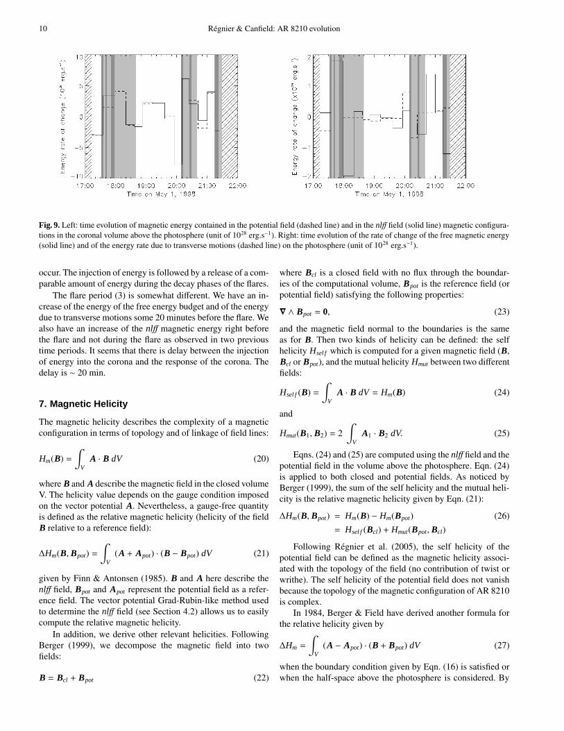
In Fig. 9 left, we plot the rate of change of the magneticenergy contained in the corona for the potential field (dashedline) and for the nlff field (solid line). We notice that the rate ofchange of the potential and nlff energies always have the samesign. We also observe that both rates are negative before theflare periods (1) and (2), for which the impulsive phase is short(< 5 min), and that the energy first increases during the flaresand then decreases during the decay phases. By integrating therates of change of energy, we conclude that at the end of thetime series more energy is stored in AR 8210 by ∼ 10%.

In Fig. 9 right, we plot the time evolution of the rates givenby Eqns. (18) and (19). The rate of change of coornal energydue to transverse motions represents how the magnetic energyis injected through the photosphere into the corona. For theflare periods (1) and (2), the energy injected through the pho-tosphere into the corona is correlated with the increase of mag-netic energy in the coronal volume at the same time as the flares


Fig. 9. Left: time evolution of magnetic energy contained in the potential field (dashed line) and in the nlff field (solid line) magnetic configura-tions in the coronal volume above the photosphere (unit of 1028 erg.s−1). Right: time evolution of the rate of change of the free magnetic energy(solid line) and of the energy rate due to transverse motions (dashed line) on the photosphere (unit of 1028 erg.s−1).

occur. The injection of energy is followed by a release of a com-parable amount of energy during the decay phases of the flares.

The flare period (3) is somewhat different. We have an in-crease of the energy of the free energy budget and of the energydue to transverse motions some 20 minutes before the flare. Wealso have an increase of the nlff magnetic energy right beforethe flare and not during the flare as observed in two previoustime periods. It seems that there is delay between the injectionof energy into the corona and the response of the corona. Thedelay is ∼ 20 min.

7. Magnetic Helicity

The magnetic helicity describes the complexity of a magneticconfiguration in terms of topology and of linkage of field lines:

Hm(B) =∫

VA · B dV (20)

where B and A describe the magnetic field in the closed volumeV. The helicity value depends on the gauge condition imposedon the vector potential A. Nevertheless, a gauge-free quantityis defined as the relative magnetic helicity (helicity of the fieldB relative to a reference field):

∆Hm(B, Bpot) =∫

V(A + Apot) · (B − Bpot) dV (21)

given by Finn & Antonsen (1985). B and A here describe thenlff field, Bpot and Apot represent the potential field as a refer-ence field. The vector potential Grad-Rubin-like method usedto determine the nlff field (see Section 4.2) allows us to easilycompute the relative magnetic helicity.

In addition, we derive other relevant helicities. FollowingBerger (1999), we decompose the magnetic field into twofields:

B = Bcl + Bpot (22)

where Bcl is a closed field with no flux through the boundar-ies of the computational volume, Bpot is the reference field (orpotential field) satisfying the following properties:

∇ ∧ Bpot = 0, (23)

and the magnetic field normal to the boundaries is the sameas for B. Then two kinds of helicity can be defined: the selfhelicity Hsel f which is computed for a given magnetic field (B,Bcl or Bpot), and the mutual helicity Hmut between two differentfields:

Hsel f (B) =∫

VA · B dV = Hm(B) (24)

and

Hmut(B1, B2) = 2∫

VA1 · B2 dV. (25)

Eqns. (24) and (25) are computed using the nlff field and thepotential field in the volume above the photosphere. Eqn. (24)is applied to both closed and potential fields. As noticed byBerger (1999), the sum of the self helicity and the mutual heli-city is the relative magnetic helicity given by Eqn. (21):

∆Hm(B, Bpot) = Hm(B) − Hm(Bpot) (26)= Hsel f (Bcl) + Hmut(Bpot, Bcl)

Following Regnier et al. (2005), the self helicity of thepotential field can be defined as the magnetic helicity associ-ated with the topology of the field (no contribution of twist orwrithe). The self helicity of the potential field does not vanishbecause the topology of the magnetic configuration of AR 8210is complex.

In 1984, Berger & Field have derived another formula forthe relative helicity given by

∆Hm =

∫

V(A − Apot) · (B + Bpot) dV (27)

when the boundary condition given by Eqn. (16) is satisfied orwhen the half-space above the photosphere is considered. By


computing both relative magnetic helicity given by the Finn &Antonsen and the Berger & Field formula, we show that the dif-ference between those two quantities is never more than 5% forthe entire time series. This fact means that the boundary con-ditions defined by the composite magnetogram (IVM + MDI)are put far enough to consider that the magnetic field vanishesat infinity required by Eqn. (15).

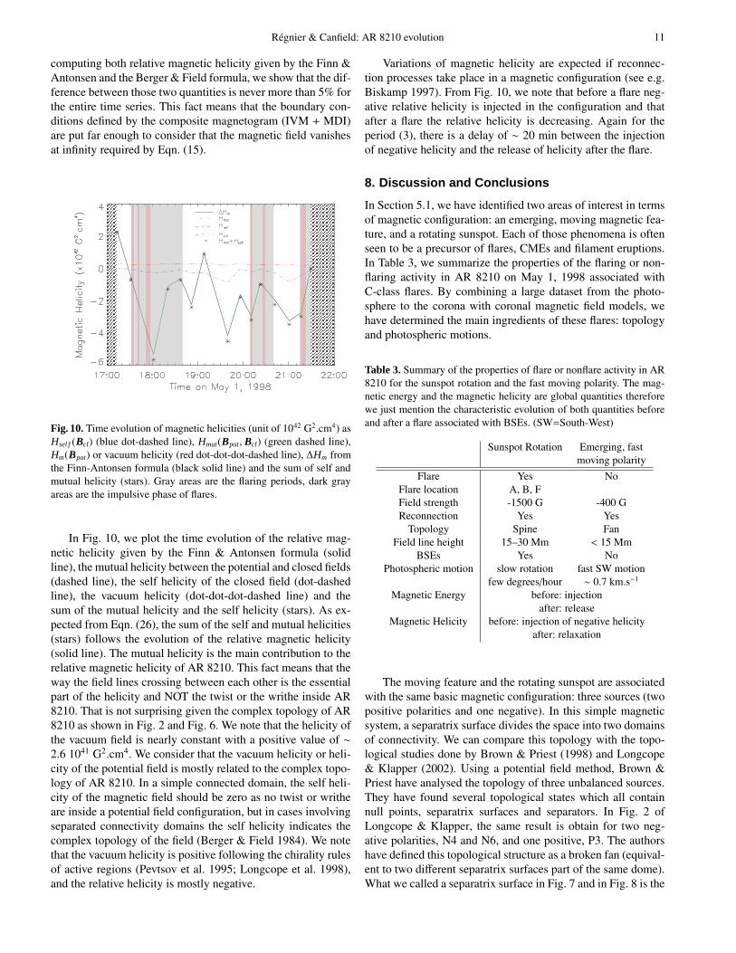
Fig. 10. Time evolution of magnetic helicities (unit of 1042 G2.cm4) asHsel f (Bcl) (blue dot-dashed line), Hmut(Bpot, Bcl) (green dashed line),Hm(Bpot) or vacuum helicity (red dot-dot-dot-dashed line), ∆Hm fromthe Finn-Antonsen formula (black solid line) and the sum of self andmutual helicity (stars). Gray areas are the flaring periods, dark grayareas are the impulsive phase of flares.

In Fig. 10, we plot the time evolution of the relative mag-netic helicity given by the Finn & Antonsen formula (solidline), the mutual helicity between the potential and closed fields(dashed line), the self helicity of the closed field (dot-dashedline), the vacuum helicity (dot-dot-dot-dashed line) and thesum of the mutual helicity and the self helicity (stars). As ex-pected from Eqn. (26), the sum of the self and mutual helicities(stars) follows the evolution of the relative magnetic helicity(solid line). The mutual helicity is the main contribution to therelative magnetic helicity of AR 8210. This fact means that theway the field lines crossing between each other is the essentialpart of the helicity and NOT the twist or the writhe inside AR8210. That is not surprising given the complex topology of AR8210 as shown in Fig. 2 and Fig. 6. We note that the helicity ofthe vacuum field is nearly constant with a positive value of ∼2.6 1041 G2.cm4. We consider that the vacuum helicity or heli-city of the potential field is mostly related to the complex topo-logy of AR 8210. In a simple connected domain, the self heli-city of the magnetic field should be zero as no twist or writheare inside a potential field configuration, but in cases involvingseparated connectivity domains the self helicity indicates thecomplex topology of the field (Berger & Field 1984). We notethat the vacuum helicity is positive following the chirality rulesof active regions (Pevtsov et al. 1995; Longcope et al. 1998),and the relative helicity is mostly negative.

Variations of magnetic helicity are expected if reconnec-tion processes take place in a magnetic configuration (see e.g.Biskamp 1997). From Fig. 10, we note that before a flare neg-ative relative helicity is injected in the configuration and thatafter a flare the relative helicity is decreasing. Again for theperiod (3), there is a delay of ∼ 20 min between the injectionof negative helicity and the release of helicity after the flare.

8. Discussion and Conclusions

In Section 5.1, we have identified two areas of interest in termsof magnetic configuration: an emerging, moving magnetic fea-ture, and a rotating sunspot. Each of those phenomena is oftenseen to be a precursor of flares, CMEs and filament eruptions.In Table 3, we summarize the properties of the flaring or non-flaring activity in AR 8210 on May 1, 1998 associated withC-class flares. By combining a large dataset from the photo-sphere to the corona with coronal magnetic field models, wehave determined the main ingredients of these flares: topologyand photospheric motions.

Table 3. Summary of the properties of flare or nonflare activity in AR8210 for the sunspot rotation and the fast moving polarity. The mag-netic energy and the magnetic helicity are global quantities thereforewe just mention the characteristic evolution of both quantities beforeand after a flare associated with BSEs. (SW=South-West)

Sunspot Rotation Emerging, fastmoving polarity

Flare Yes NoFlare location A, B, FField strength -1500 G -400 GReconnection Yes Yes

Topology Spine FanField line height 15–30 Mm < 15 Mm

BSEs Yes NoPhotospheric motion slow rotation fast SW motion

few degrees/hour ∼ 0.7 km.s−1

Magnetic Energy before: injectionafter: release

Magnetic Helicity before: injection of negative helicityafter: relaxation

The moving feature and the rotating sunspot are associatedwith the same basic magnetic configuration: three sources (twopositive polarities and one negative). In this simple magneticsystem, a separatrix surface divides the space into two domainsof connectivity. We can compare this topology with the topo-logical studies done by Brown & Priest (1998) and Longcope& Klapper (2002). Using a potential field method, Brown &Priest have analysed the topology of three unbalanced sources.They have found several topological states which all containnull points, separatrix surfaces and separators. In Fig. 2 ofLongcope & Klapper, the same result is obtain for two neg-ative polarities, N4 and N6, and one positive, P3. The authorshave defined this topological structure as a broken fan (equival-ent to two different separatrix surfaces part of the same dome).What we called a separatrix surface in Fig. 7 and in Fig. 8 is the


projection on the photospheric plane of the separatrix surface(including the separator field line) dividing the broken fan intotwo domains of connectivity. For the moving feature, the topo-logical element dividing the domains is the fan surface. For therotating sunspot, the spine field line has the same photosphericfootprint as the separatrix surface. Those types of reconnectioncan be fast as shown by Parnell & Galsgaard (2004).

In both the moving feature and the sunspot rotation, the ori-gins of reconnections lie in the photospheric motions of fieldlines footpoints. For the moving feature, the parasitic polarityemerges into the pre-existing three-source magnetic configur-ation and the fast displacement of this polarity leads to smallreconnection processes. For the sunspot rotation, the field linesexisting in the three-source configuration are moved toward theseparatrix surface by the clockwise rotation and generate re-connections.

In this article, we have focused our study on small eruptiveevents which did not dramatically modify the magnetic config-uration of the active region. In this study the most importantingredient is to use a good time series of vector magnetogramsbefore and after flaring activity. A similar study can be donefor M or X-class flares with the development of vector mag-netic field measurements on the photosphere or in the chromo-sphere by Solar B/SOT (Solar Optical Telescope), SDO/HMI(Helioseismic and Magnetic Imager) or ground-based obser-vatories (MSO, NSO/SOLIS, THEMIS, GREGOR, HuairouObservatory).

Acknowledgements. The authors would like to thank M. Berger, D.McKenzie, D. Longcope and G. Fisher for fruitful discussions andcomment as well as Mees Solar Observatory observers who haveprovided us the IVM observations. S. R. research is funded by theEuropean Commission’s Human Potential Programme through theEuropean Solar Magnetism Network, and by AFOSR under a DoDMURI grant ”Understanding Solar Eruptions and Their InterplanetaryConsequences”.

References

Amari, T., Aly, J. J., Luciani, J. F., Boulmezaoud, T. Z., &Mikic, Z. 1997, Solar Phys., 174, 129

Amari, T., Boulmezaoud, T. Z., & Mikic, Z. 1999, A&A, 350,1051

Antiochos, S. K. 1987, ApJ, 312, 886Berger, M. A. 1999, in Magnetic Helicity in Space and

Laboratory Plasmas (Brown, M. R., Canfield, R. C., Pevtsov,A. A. Eds), 1–9

Berger, M. A. & Field, G. B. 1984, Journal of Fluid Mechanics,147, 133

Biskamp, D. 1997, Nonlinear Magnetohydrodynamics(Nonlinear Magnetohydrodynamics, ISBN 0521599180,Cambridge University Press, Paperback, 1997.)

Bleybel, A., Amari, T., van Driel-Gesztelyi, L., & Leka, K. D.2002, A&A, 395, 685

Brown, D. S., Nightingale, R. W., Alexander, D., et al. 2003,Solar Phys., 216, 79

Brown, D. S. & Priest, E. R. 1998, in ASP Conf. Ser. 155:Three-Dimensional Structure of Solar Active Regions, 90

Canfield, R. C., de La Beaujardiere, J.-F., Fan, Y., et al. 1993,ApJ, 411, 362

Canfield, R. C. & Reardon, K. P. 1998, Solar Phys., 182, 145Carmichael, H. 1964, in AAS–NASA Symp. on Physics of

Solar Flares, 451Delaboudiniere, J.-P., Artzner, G. E., Brunaud, J., et al. 1995,

Solar Phys., 162, 291Des Jardins, A. C. & Canfield, R. C. 2003, ApJ, 598, 678Finn, J. M. & Antonsen, T. M. 1985, Comments Plasma Phys.

Controlled Fusion, 9, 111Fletcher, L., Metcalf, T. R., Alexander, D., Brown, D. S., &

Ryder, L. A. 2001, ApJ, 554, 451Georgoulis, M. K. & LaBonte, B. J. 2005, ApJ, submittedGrad, H. & Rubin, H. 1958, in Proc. 2nd Int. Conf. on Peaceful

Uses of Atomic Energy, Geneva, United Nations, Vol. 31,190

Hirayama, T. 1974, Solar Phys., 34, 323Ishii, T. T., Kurokawa, H., & Takeuchi, T. T. 1998, ApJ, 499,

898Kopp, R. A. & Pneuman, G. W. 1976, Solar Phys., 50, 85Kusano, K., Maeshiro, T., Yokoyama, T., & Sakurai, T. 2002,

ApJ, 577, 501Kucera, A. 1982, Bull. Astron. Inst. Czechosl., 33, 345LaBonte, B. J., Mickey, D. L., & Leka, K. D. 1999, Solar Phys.,

189, 1Landolfi, M. & Degl’innocenti, E. L. 1982, Solar Phys., 78, 355Leka, K. D. 1999, Solar Phys., 188, 21Leka, K. D. & Skumanich, A. 1999, Solar Phys., 188, 3Lin, J., Soon, W., & Baliunas, S. L. 2003, New Astronomy

Review, 47, 53Lin, Y. & Chen, J. 1989, Chinese Journal of Space Science, 9,

206Livi, S. H. B., Martin, S., Wang, H., & Ai, G. 1989, Solar Phys.,

121, 197Longcope, D. W. 2004, ApJ, 612, 1181Longcope, D. W., Fisher, G. H., & Pevtsov, A. A. 1998, ApJ,

507, 417Longcope, D. W. & Klapper, I. 2002, ApJ, 579, 468Mickey, D. L., Canfield, R. C., Labonte, B. J., et al. 1996, Solar

Phys., 168, 229Mikic, Z. & McClymont, A. N. 1994, in ASP Conf. Ser. 68:

Solar Active Region Evolution: Comparing Models withObservations, 225

Moon, Y.-J., Chae, J., Wang, H., Choe, G. S., & Park, Y. D.2002, ApJ, 580, 528

Nightingale, R. W., Brown, D. S., Metcalf, T. R., et al. 2002,in Multi-Wavelength Observations of Coronal Structure andDynamics, 149

Nindos, A. & Zhang, H. 2002, ApJ, 573, L133November, L. J. & Simon, G. W. 1988, ApJ, 333, 427Parnell, C. E. & Galsgaard, K. 2004, A&A, 428, 595Penn, M. J., Mickey, D. L., Canfield, R. C., & Labonte, B. J.

1991, Solar Phys., 135, 163Pevtsov, A. A., Canfield, R. C., & Metcalf, T. R. 1995, ApJ,

440, L109Pohjolainen, S., Maia, D., Pick, M., et al. 2001, ApJ, 556, 421Priest, E. & Forbes, T., eds. 2000, Magnetic reconnection :

MHD theory and applications


Priest, E. R. & Forbes, T. G. 2002, A&A Rev., 10, 313Regnier, S. & Amari, T. 2004, A&A, 425, 345Regnier, S., Amari, T., & Canfield, R. C. 2005, A&A, in pressRegnier, S. 2001, PhD ThesisRegnier, S., Amari, T., & Kersale, E. 2002, A&A, 392, 1119Regnier, S. & Canfield, R. C. 2004, in SOHO 15: Coronal

Heating, ESA-SP 575Sakurai, T. 1982, Solar Phys., 76, 301Scherrer, P. H., Bogart, R. S., Bush, R. I., et al. 1995, Solar

Phys., 162, 129Schmieder, B., Aulanier, G., Demoulin, P., et al. 1997, A&A,

325, 1213Sterling, A. C. & Moore, R. L. 2001a, ApJ, 560, 1045Sterling, A. C. & Moore, R. L. 2001b, J. Geophys. Res., 25227Sterling, A. C., Moore, R. L., Qiu, J., & Wang, H. 2001, ApJ,

561, 1116Sturrock, P. A. 1968, in IAU Symp. 35: Structure and

Development of Solar Active Regions, 471Thompson, B. J., Cliver, E. W., Nitta, N., Delannee, C., &

Delaboudiniere, J.-P. 2000, Geophys. Res. Lett., 27, 1431Tsuneta, S., Acton, L., Bruner, M., et al. 1991, Solar Phys.,

136, 37Unno, W. 1956, PASJ, 8, 108Wang, T., Yan, Y., Wang, J., Kurokawa, H., & Shibata, K. 2002,

ApJ, 572, 580Warmuth, A., Hanslmeier, A., Messerotti, M., et al. 2000, Solar

Phys., 194, 103Welsch, B. T., Fisher, G. H., Abbett, W. P., & Regnier, S. 2004,

ApJ, 610, 1148Wheatland, M. S., Sturrock, P. A., & Roumeliotis, G. 2000,

ApJ, 540, 1150Wiegelmann, T. 2004, Sol. Phys., 219, 87Xia, Z. G., Wang, M., Zhang, B. R., & Yan, Y. H. 2001, Acta

Astronomica Sinica, 42, 357Yan, Y. & Sakurai, T. 2000, Solar Phys., 195, 89Yan, Y. & Wang, J. 1995, A&A, 298, 277Zhang, J. & Wang, J. 2001, ApJ, 554, 474

Evolution of magnetic ﬁelds and energetics of ﬂares in ...

Documents

Transcript of Evolution of magnetic ﬁelds and energetics of ﬂares in ...