Analysis and modelling of recurrent solar ﬂares observed ... · Analysis and modelling of...

Astronomy & Astrophysics manuscript no. Printer˙version˙corrections˙arxiv c© ESO 2018June 18, 2018

Analysis and modelling of recurrent solar flares observed withHinode/EIS on March 9, 2012

V. Polito1, G. Del Zanna1, G. Valori2, E. Pariat3, H. E. Mason1, J. Dudık4, and M. Janvier5

1 Department of Applied Mathematics and Theoretical Physics, CMS, University of Cambridge, Wilberforce Road,Cambridge CB3 0WA, United Kingdom e-mail: [email protected]

2 UCL Mullard Space Science Laboratory, Holmbury St. Mary, Dorking, Surrey RH5 6NT, UK,3 LESIA, Observatoire de Paris, PSL Research University, CNRS, Sorbonne Universits, UPMC Univ. Paris 06, Univ. Paris Diderot,

Sorbonne Paris Cit, 5 place Jules Janssen, 92195 Meudon, France4 Astronomical Institute, Academy of Sciences of the Czech Republic, 25165 Ondrejov, Czech Republic,5 Institut d’Astrophysique Spatiale, CNRS, Univ. Paris-Sud, Universit Paris-Saclay, B¢t. 121, 91405 Orsay cedex, France

Preprint online version: June 18, 2018

ABSTRACT

Three homologous C-class flares and one last M-class flare were observed by both the Solar Dynamics Observatory (SDO) andthe Hinode EUV Imaging Spectrometer (EIS) in the AR 11429 on March 9, 2012. All the recurrent flares occurred within a shortinterval of time (less than 4 hours), showed very similar plasma morphology and were all confined, until the last one when a large-scale eruption occurred. The C-class flares are characterized by the appearance, at approximatively the same locations, of two brightand compact footpoint sources of ≈ 3–10 MK evaporating plasma, and a semi-circular ribbon. During all the flares, the continuousbrightening of a spine-like hot plasma (≈ 10 MK) structure is also observed. Spectroscopic observations with Hinode/EIS are used tomeasure and compare the blueshift velocities in the Fe XXIII emission line and the electron number density at the flare footpoints foreach flare. Similar velocities, of the order of 150–200 km s−1, are observed during the C2.0 and C4.7 confined flares, in agreementwith the values reported by other authors in the study of the last M1.8 class flare. On the other hand, lower electron number densitiesand temperatures tend to be observed in flares with lower peak soft X-ray flux. In order to investigate the homologous nature of theflares, we performed a Non-Linear Force-Free Field (NLFFF) extrapolation of the 3D magnetic field configuration in the corona. TheNLFFF extrapolation and the Quasi-Separatrix Layers (QSLs) provide the magnetic field context which explains the location of thekernels, spine-like and semi-circular brightenings observed in the (non-eruptive) flares. Given the absence of a coronal null point, weargue that the homologous flares were all generated by the continuous recurrence of bald patch reconnection.

Key words. Sun: flares, UV radiation – Techniques: spectroscopic – Magnetic fields – Methods: numerical

1. Introduction

Although major observational advances and significant progressin theoretical modelling have been achieved in the last fewdecades, we still lack a definitive model for solar flares. The stan-dard model of flares in 2D (CSHKP; Carmichael 1964; Sturrock1968; Hirayama 1974; Kopp & Pneuman 1976) proposes thatflares are driven by magnetic reconnection in the corona. Theenergy release due to reconnection results in heating of the localplasma, bulk kinetic energy and wave generation, although it isstill unclear how the energy is partitioned between different pro-cesses. In all cases, the energy is transported towards the chro-mosphere at the flare footpoints also called kernels, where theplasma is heated to very high temperatures (above 10 MK), and,due to the overpressure, evaporates along the field lines (chro-mospheric evaporation). The 2D model succeeds in explainingthe observed chromospheric brightenings and high temperatureupflows at the flare footpoints, as well as particle accelerationand the thermal cooling of loops. However, it fails to reproducesome more detailed features which can only be explained by 3Dmodels of eruptive flares, such as the strong-to-weak evolutionof the shear of flare loops (Aulanier et al. 2012), the apparentslipping motion of the flare footpoints (Janvier et al. 2013; Dudıket al. 2014, 2016) and the J-shaped structure of the ribbons (see,e.g. Janvier et al. 2015, and references therein). Also, in the 3D

models, magnetic reconnection can happen even in the absenceof a null point: rather it is associated with finite-volume regionswhere the magnetic connectivity is characterized by strong gra-dients, called quasi-separatrix layers (QSLs; Priest & Demoulin1995; Demoulin et al. 1996; Titov et al. 2002). While there isa general consensus on magnetic reconnection being the energyrelease mechanism for flares, the details of the energy conver-sion and transport through the corona are still strongly debated.Comparing the theoretical models with observations is compli-cated by the fact that we cannot observe the energy release di-rectly. A possible approach to this problem is to observe theresult of the heating, that is, plasma observables in EUV andX-ray wavelengths (such as flows, density, temperature, emis-sion measure, electron distribution). Several authors have com-pared observations with modelling in order to infer evidencesupporting a particular flare model, between thermal conduc-tion, thick-target or Afvenic wave models (see e.g. Petkaki et al.2012; Doschek et al. 2015; Battaglia et al. 2015; Polito et al.2016). One of the key observables is the blueshift of spectrallines revealing upflows at the loop footpoints during the chro-mospheric evaporation phase. This was first observed in the softX-ray lines with SOLFLEX (Doschek et al. 1979) and the SolarMaximum Mission (SMM) (Antonucci et al. 1982). These lines(8–25 MK) showed strong blue-asymmetric profiles, in contrastto the theoretical predictions of completely blueshifted line pro-

1

arX

iv:1

612.

0350

4v1

[as

tro-

ph.S

R]

12

Dec

201

6

V. Polito et al.: Analysis and modelling of recurrent solar flares observed with Hinode/EIS on March 9, 2012

files (Emslie & Alexander 1987). The chromospheric evapora-tion phase in flares has subsequently been extensively observedwith the Coronal Diagnostic Spectrometer (CDS; Harrison et al.1995) on board SoHO and the EUV Imaging Spectrometer (EIS;Culhane et al. 2007) on board Hinode. Similar to the earlier stud-ies, many CDS and EIS observations (e.g., Teriaca et al. 2003;Brosius 2003; Milligan et al. 2006) still showed strong asym-metries in the high temperature line profiles (Fe XIX with CDS,Fe XXIII and Fe XXIV with EIS). These asymmetries were of-ten interpreted as being due to a superposition of plasma up-flows at different velocities along the line-of-sight (Warren &Doschek 2005; Reeves et al. 2007). Totally shifted symmetri-cal profiles were however sometimes observed (Del Zanna et al.2006, 2011a; Brosius 2013), in agreement with theory. Our un-derstanding of chromospheric evaporation has been consider-ably improved since the launch of the IRIS satellite (De Pontieuet al. 2014) in 2013. In particular, simultaneous joint observa-tions with both EIS (in Fe XXIII) and IRIS (in Fe XXI) haveconfirmed that the asymmetric profiles seen with EIS are mostlydue to the limited spatial resolution of EIS, since IRIS observedtotally shifted Fe XXI profiles during all the observation(Politoet al. 2016). On the other hand, compared to IRIS, EIS hasthe advantage of observing many spectral lines formed at coro-nal and flare temperatures, which can provide useful plasmadiagnostics during flares (see e.g. the observational review byMilligan 2015). For instance, in the observation of a small B-class flare by Del Zanna et al. (2011a), the authors reported acomprehensive study of chromospheric evaporation, cooling andevolution of the plasma based on the analysis of several spectrallines with EIS.

One of the unsolved questions in solar flare models is un-derstanding if the same mechanism is responsible for large andsmall size events. Kahler (1982) suggested that there is a statisti-cal correlation between solar flare energy release and the magni-tude of any measured flare energy manifestation. Several statisti-cal studies have been dedicated to comparing the plasma param-eters of a large number of flares over time (e.g. Feldman et al.1996; Battaglia et al. 2005; Hannah et al. 2011). For instance,Feldman et al. (1996) studied the correlation between soft X-rayflare class and emission measure with electron temperature for868 flares of X-ray class A2 to X2. They found that the logar-itmic of the flux measure in GOES 1–8 Å or 0.5–4 Å channelsand the EM measured by either detectors is linearly proportionalto the electron temperature.

It should be noted that flare events happening in very dif-ferent plasma environments are difficult to compare directly. Infact, each flare can show different plasma parameters becauseof the different initial conditions in the active region where itoccurred. The so-called recurrent or homologous flares are par-ticularly interesting events, where a similar magnetic field con-figuration is reformed over time. Several authors have focusedon analysing the magnetic field structure and evolution in recur-rent flares. Some of the studies suggest that the flares are causedby the continuous emergence of new magnetic flux in the ac-tive region (e.g Nitta & Hudson 2001). Other authors concludedthat persistent shearing motions could trigger the energy releasein homologous flares (e.g. Romano et al. 2015). Although thereare several imaging and magnetic field observations of recurrentflares, there have not been many spectroscopic observations todate. One of the main issues is associated with the difficulty ofobserving the exact location of the flare footpoints for a longperiod of time within the limited field-of-view of spectroscopicinstruments.

A sequence of 4 recurrent flares in the Active Region NOAA11429 was observed by EIS on the 9 March 2012. EIS wasin a raster mode and could observe both flare loop footpoints.Spectroscopic observations of recurrent flares in the same activeregion (and covering both footpoint locations) offer the uniquepossibility of comparing the physical observables in flares of dif-ferent size taking place in a similar plasma environment. In par-ticular, we aim to address the following questions:

– How do the plasma parameters (flows, density, temperature)vary in flares of increasing energy?

– Is there a difference in the upflows observed at the two foot-points during the chromospheric evaporation phase?

– How does the timing of the EIS observations (slit positionduring the raster) affect the measurement of the upflows dur-ing the chromospheric evaporation process?

– What causes the homologous flares and how does the mag-netic field structure evolve?

The first three questions can be addressed by combiningmulti-wavelength imaging from the SDO/Atmospheric ImagingAssembly (AIA; Boerner et al. 2012) with spectroscopic ob-servations from EIS. In order to study the magnetic field struc-ture during the recurrent flares, we analysed data from theSDO/Helioseismic and Magnetic Imager (HMI; Scherrer et al.2012) and performed a Non Linear Force-Free Field (NLFFF)extrapolation in the active region under study.

The paper is structured as follows: Sect. 2 introduces thecontext of the AIA and EIS observations and the flare events.A detailed analysis of the blueshifts observed by EIS is then pre-sented in Sect. 3. Sect. 4 and 5 provide density and temperaturediagnostics based on the use of spectroscopic and imaging data.An analysis of the magnetic topology of the active region dur-ing the recurrent flares and the results of the extrapolation arethen presented in Sect. 6. Finally, we discuss and summarize ourresults in Sect. 7.

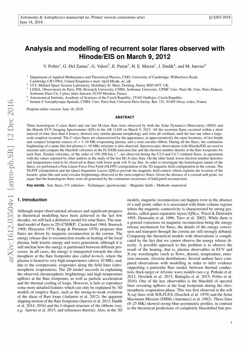
Fig. 1. Soft X-ray light curves of the recurrent flares on March9, 2012 observed by GOES in the 0.5–4 Å and 1–8 Å chan-nels. The vertical dotted lines indicate the time of the EIS rastersthat we analysed in this work, as explained in Sect. 2.2. The redarrows indicate the period of time when EIS was observing theflaring AR. See text for more details.

2


Fig. 2. Overview of the C-class recurrent flares on 9 March 2012 as observed by AIA in the following channels: 304 (left column),171 (middle) and 131 Å (right). The field-of-view of the EIS spectrometer is indicated by the yellow (and white in the middlecolumn) boxes in the figure. In addition, the location of the footpoint K1 and K2 (see Sect. 3) are indicated on the 304 image on thethird row. Finally, the small white arrows in the 131 Å image in the third, fifth and sixth rows row indicate: the spine-like feature,the erupting flux rope, and the slipping motion of the southern flare ribbon respectively, as discussed in the text. The online Movies1 and 2 show the evolution of the 171 and 131 Å AIA images respectively over time. See text for discussion of the rows.

Table 1. Time of the recurrent flares as observed by GOES

Flare Start Peak End Observed by EIS(UT) (UT) (UT)

C1.0 00:34 00:37 00:46 yesC2.0 01:23 01:28 01:34 yesC4.7 01:55 02:00 02:06 yesC1.2 03:01 03:04 03:08 no

M1.8/6.3 03:22 03:27/03:53 04:18 yes

2. Spectroscopic and imaging observations of therecurrent flares

Active Region (AR) NOAA 11429 was a highly complex βγδregion which produced many energetic events during the inter-val March 7–11, 2012. The magnetic evolution of this regionwas analysed by several authors (e.g. Chintzoglou et al. 2015a;Syntelis et al. 2016; Kouloumvakos et al. 2016; Patsourakoset al. 2016a).

A sequence of five recurrent flares occurred in the AR 11429on March 9, 2012 from around 00:00 UT to 04:18 UT, as shownin the GOES light curves in Fig. 1. The first four C-class flares(C1.0, C2.0, C4.7 and C1.2) were all confined. The last M-classeruptive flare started at 03:22 UT, reached a first maximum inthe soft X-ray flux at around 03:27 UT (M1.8 class) and, after

3


two small dips in intensity, increased up to about M6.3 (see Fig.1). EIS observed three of the C-class flares and the first part ofthe M-class flare, as indicated by the red arrows in Fig. 1.

The M-class flare is a well-studied event. A detailed anal-ysis of the EIS observations of the M1.8 flare was presentedby Doschek et al. (2013). This eruptive flare was also studiedby Simoes et al. (2013), who analysed the strong contractingmotions of peripheral coronal loops during the flare impulsivephase. In addition, Hao et al. (2012) focused on studying thewhite-light emission produced during the flare.

In this work we mainly focus on the series of three C-classconfined flares observed before the M-class flare by EIS. Thevertical dotted lines in Fig. 1 indicate the times of the EIS rasterswhich were analysed in this work. The start, peak, and end timesof all the flares are summarized in Tab. 1.

Sect. 2.1 provides an overview of the homologous flares(including the last eruptive one), as observed in the SDO/AIAmulti-wavelength images. Sect. 2.2 presents the details of theEIS spectroscopic observation of the three C-class confinedflares.

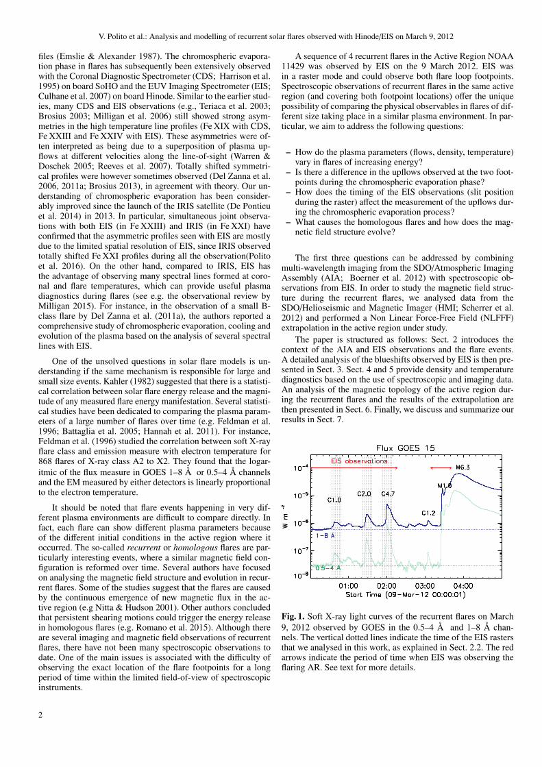
Fig. 3. SDO/HMI BLOS image of the AR 11429 during thepeak of the C4.7 class flare. The intensity contours of the AIA304 Å image of the flare are overplot in red. The position ofthe flare footpoints K1 and K2 (see Sect. 3) are also indicated,showing that the two footpoints are located in different magneticpolarities. The field-of-view of the AIA images in Fig. 4 is over-laid as a black boxed area.

2.1. AIA and HMI observation

The SDO/AIA and SDO/HMI magnetograms data were down-loaded through the solarsoft VSO package and converted to level1.5 images using the aia prep and hmi prep routines, respec-tively. The images were also corrected for solar rotation andaligned with the EIS images, as described in Sect. 2.2.

Fig. 2 shows an overview of the AIA observation of thehomologous flares in the 304 (left), 171 (middle) and 131(right) Å filters. During flares, these filters are dominated byemission from plasma at ≈ 0.05 MK, 1 MK and 11 MK respec-tively (e.g. O’Dwyer et al. 2010; Del Zanna et al. 2011b). Theonline Movies 1 and 2 show the evolution of the recurrent flares

over time, as observed by the 171 Å and 131 Å filters respec-tively.

The first row of Fig. 2 shows the first C1.0 class flare justafter the peak, at around 00:38 UT. The flare ribbons can best beseen in the low temperature 304 Å image, while the 131 Å im-age shows the high temperature flare loops (≈ 10 MK). The304 Å image also shows an elongated and dark filament struc-ture following the polarity inversion line (PIL) along the wholeAR. Notice that the filament appears to be composed of severalsegments which are constantly present until the major eruptionoccurs during the M-class flare. While the western arm has a sin-gle U-structure, the eastern arm extends northward as a collec-tion of smaller fragments. The observations —including those atother wavelengths— do not allow us to discern if the fragmenta-tion corresponds to an equally fragmented magnetic structure orrather is the effect of irregular absorption along the filament.

The second row in Fig. 2 shows the second C2.0 class flare,while the peak of the C4.7 class flare (at around 02:00 UT) isshown in the third row, with the field-of-view of the EIS spec-trometer overlaid (indicated by the coloured yellow and whiteboxes). In order to better understand the context of the observedevent, the intensity contours of the 304 Å AIA image around02:00 UT are overlaid on the the line-of-sight magnetic field(BLOS) map observed with SDO/HMI in Fig. 3. The overlayshows the complex morphology of the flare ribbons, with thenegative polarity ribbon having a semi-circular shape. We canalso observe two bright emission sources in the AIA 304 Å inten-sity contours, which are located on opposite magnetic polaritiesand indicated as K1 and K2 in Figs. 2 and 3. We indicate thesefootpoint sources as kernels, since they represent the locationwhere the chromospheric evaporation takes place (in the contextof the 2D standard flare model) as better described in Sects. 2.2and 3. This interpretation is corroborated by the simultaneity ofthe appearance of the two kernels in all 3 C-class flares (Fig. 2and online Movie 1), which indicates that the two locations aremagnetically connected by loops created during the flare events.

Fig. 2 also shows the presence of a spine-like feature, whichis indicated by the white arrow in the 131 Å image at around02:00 UT (third row). This feature is observed to brighten upduring all the recurrent flares. A more detailed analysis of themagnetic field structure associated with these features will bepresented in Sect. 6.

The AIA images in the fourth row of Fig. 2 show the eruptiveM-class flare just after its peak. In these images we note that theflare loops and the bright spine-like structure form at approxi-mately the same location as the confined flares.

2.2. EIS observation

On the 9 March 2012, EIS was running a core flare tr120x120study from around 00:02:39 UT to 02:16:04 UT on the AR11429, observing the sequence of the three C-class homolo-gous flares over a field-of-view of 120′′ × 120′′. From around03:09:33 UT, the spectrometer then run an Atlas 30 full-spectrum study and caught the last eruptive M1.8 class flare. Thetiming of core flare tr120x120 and Atlas 30 observing studies isindicated respectively by the first and second (from left to right)red arrows in Fig. 1. The Atlas 30 study was analysed in detailby Doschek et al. (2013). In the following, we will focus on thespectroscopic analysis of the first three confined flares but alsocompare our results with the diagnostics reported by Doscheket al. (2013). The EIS core flare tr120x120 study is a large rasterincluding 30 × 2′′ slit positions with a jump of 1′′ between each

4


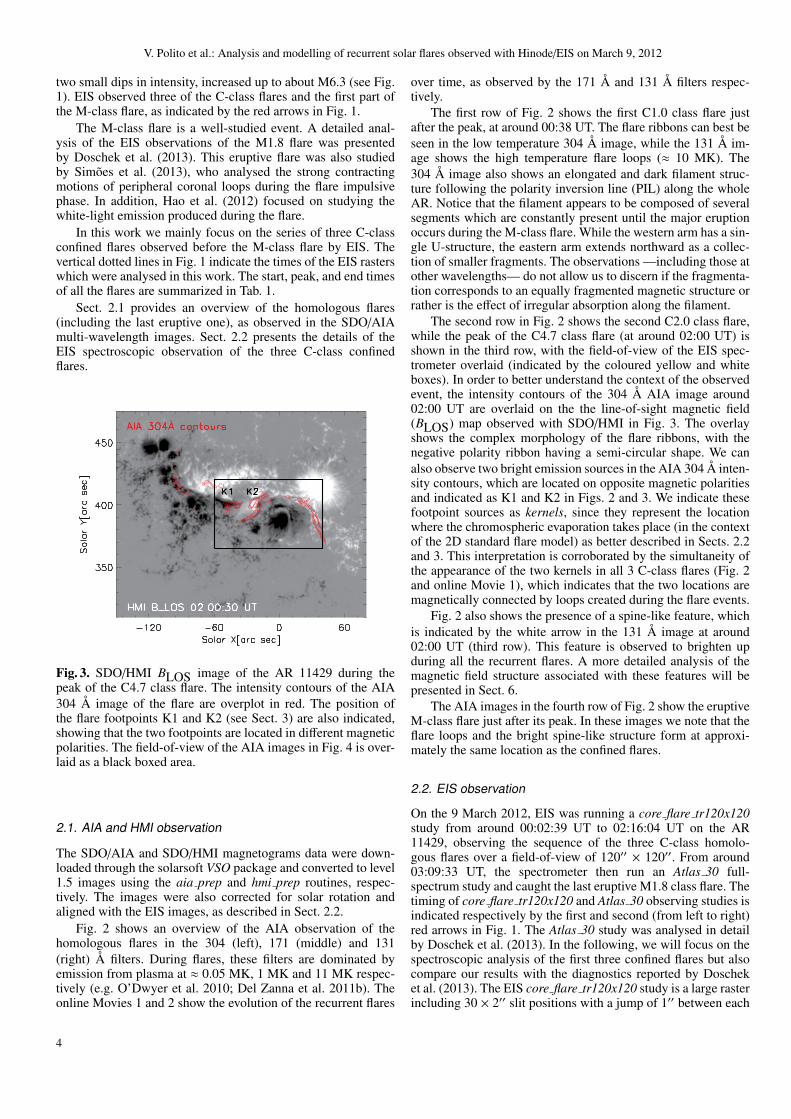
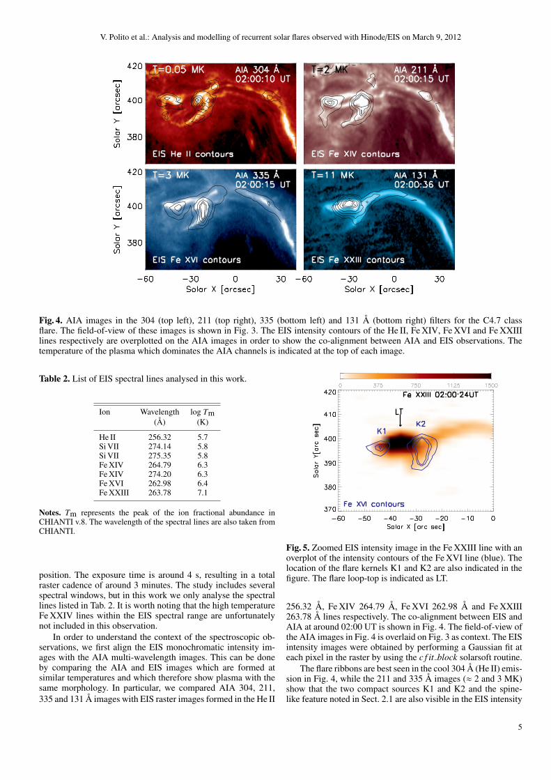
Fig. 4. AIA images in the 304 (top left), 211 (top right), 335 (bottom left) and 131 Å (bottom right) filters for the C4.7 classflare. The field-of-view of these images is shown in Fig. 3. The EIS intensity contours of the He II, Fe XIV, Fe XVI and Fe XXIIIlines respectively are overplotted on the AIA images in order to show the co-alignment between AIA and EIS observations. Thetemperature of the plasma which dominates the AIA channels is indicated at the top of each image.

Table 2. List of EIS spectral lines analysed in this work.

Ion Wavelength log Tm(Å) (K)

He II 256.32 5.7Si VII 274.14 5.8Si VII 275.35 5.8Fe XIV 264.79 6.3Fe XIV 274.20 6.3Fe XVI 262.98 6.4Fe XXIII 263.78 7.1

Notes. Tm represents the peak of the ion fractional abundance inCHIANTI v.8. The wavelength of the spectral lines are also taken fromCHIANTI.

position. The exposure time is around 4 s, resulting in a totalraster cadence of around 3 minutes. The study includes severalspectral windows, but in this work we only analyse the spectrallines listed in Tab. 2. It is worth noting that the high temperatureFe XXIV lines within the EIS spectral range are unfortunatelynot included in this observation.

In order to understand the context of the spectroscopic ob-servations, we first align the EIS monochromatic intensity im-ages with the AIA multi-wavelength images. This can be doneby comparing the AIA and EIS images which are formed atsimilar temperatures and which therefore show plasma with thesame morphology. In particular, we compared AIA 304, 211,335 and 131 Å images with EIS raster images formed in the He II

Fig. 5. Zoomed EIS intensity image in the Fe XXIII line with anoverplot of the intensity contours of the Fe XVI line (blue). Thelocation of the flare kernels K1 and K2 are also indicated in thefigure. The flare loop-top is indicated as LT.

256.32 Å, Fe XIV 264.79 Å, Fe XVI 262.98 Å and Fe XXIII263.78 Å lines respectively. The co-alignment between EIS andAIA at around 02:00 UT is shown in Fig. 4. The field-of-view ofthe AIA images in Fig. 4 is overlaid on Fig. 3 as context. The EISintensity images were obtained by performing a Gaussian fit ateach pixel in the raster by using the c f it block solarsoft routine.

The flare ribbons are best seen in the cool 304 Å (He II) emis-sion in Fig. 4, while the 211 and 335 Å images (≈ 2 and 3 MK)show that the two compact sources K1 and K2 and the spine-like feature noted in Sect. 2.1 are also visible in the EIS intensity

5


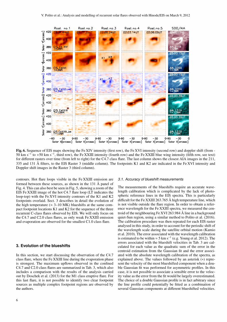
Fig. 6. Sequence of EIS maps showing the Fe XIV intensity (first row), the Fe XVI intensity (second row) and doppler shift (from -50 km s−1 to +50 km s−1, third row), the Fe XXIII intensity (fourth row) and the Fe XXIII blue wing intensity (fifth row, see text)for different rasters over time (from left to right) for the C4.7 class flare. The last column shows the closest AIA images in the 211,335 and 131 Å filters, to the EIS Raster 3 (middle column). The footpoints K1 and K2 are indicated in the Fe XVI intensity andDoppler shift images in the Raster 3 (third column).

contours. Hot flare loops visible in the Fe XXIII emission areformed between these sources, as shown in the 131 Å panel ofFig. 4. This can also best be seen in Fig. 5, showing a zoom of theEIS Fe XXIII image of the hot C4.7 flare loop (LT indicates theloop-top) with the Fe XVI intensity contours of the K1 and K2footpoints overlaid. Sect. 3 describes in detail the evolution ofthe high temperature (≈ 3–10 MK) blueshifts at the same com-pact footpoint locations K1 and K2 for the sequence of the threerecurrent C-class flares observed by EIS. We will only focus onthe C4.7 and C2.0 class flares, as only weak Fe XXIII emissionand evaporation are observed for the smallest C1.0 class flare.

3. Evolution of the blueshifts

In this section, we start discussing the observation of the C4.7class flare, where the Fe XXIII line during the evaporation phaseis strongest. The maximum upflows observed in the confinedC4.7 and C2.0 class flares are summarized in Tab. 3, which alsoincludes a comparison with the results of the analysis carriedout by Doschek et al. (2013) for the M1 class eruptive flare. Forthis last flare, it is not possible to identify two clear footpointsources as multiple complex footpoint regions are observed bythe authors.

3.1. Accuracy of blueshift measurements

The measurements of the blueshifts require an accurate wave-length calibration which is complicated by the lack of photo-spheric reference lines in the EIS spectra. This is particularlydifficult for the Fe XXIII 263.765 Å high temperature line, whichis not visible outside the flare region. In order to obtain a refer-ence wavelength for the Fe XXIII spectra, we measured the cen-troid of the neighbouring Fe XVI 263.984 Å line in a backgroundquiet-Sun region, using a similar method to Polito et al. (2016).The calibration procedure was then repeated for each EIS rasteranalysed in this study, in order to account for the periodic shift ofthe wavelength scale during the satellite orbital motion (Kamioet al. 2010). The error associated with the wavelength calibrationis estimated to be within ≈ 5 km s−1 (e.g. Young et al. 2012). Theerrors associated with the blueshift velocities in Tab. 3 are cal-culated for each value as the quadratic sum of the error in thecentroid estimation from the Gaussian fit and the error associ-ated with the absolute wavelength calibration of the spectra, asexplained above. The values followed by an asterisk (∗) repre-sent the velocity of the most blueshifted component when a dou-ble Gaussian fit was performed for asymmetric profiles. In thiscase, it is not possible to associate a sensible error to the veloc-ity value as the error from the fit would be largely overestimated.The choice of a double Gaussian profile is in fact arbitrary sincethe line profile could potentially be fitted as a combination ofseveral Gaussian components at different blueshifted velocities.

6


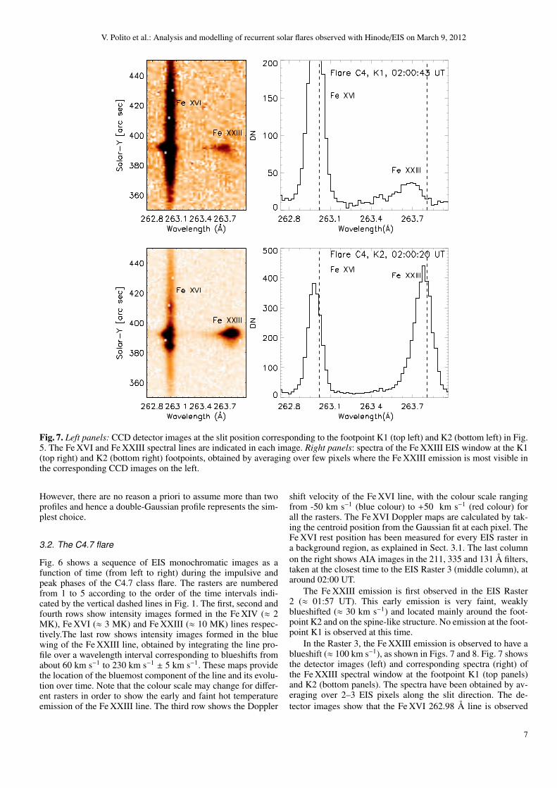
Fig. 7. Left panels: CCD detector images at the slit position corresponding to the footpoint K1 (top left) and K2 (bottom left) in Fig.5. The Fe XVI and Fe XXIII spectral lines are indicated in each image. Right panels: spectra of the Fe XXIII EIS window at the K1(top right) and K2 (bottom right) footpoints, obtained by averaging over few pixels where the Fe XXIII emission is most visible inthe corresponding CCD images on the left.

However, there are no reason a priori to assume more than twoprofiles and hence a double-Gaussian profile represents the sim-plest choice.

3.2. The C4.7 flare

Fig. 6 shows a sequence of EIS monochromatic images as afunction of time (from left to right) during the impulsive andpeak phases of the C4.7 class flare. The rasters are numberedfrom 1 to 5 according to the order of the time intervals indi-cated by the vertical dashed lines in Fig. 1. The first, second andfourth rows show intensity images formed in the Fe XIV (≈ 2MK), Fe XVI (≈ 3 MK) and Fe XXIII (≈ 10 MK) lines respec-tively.The last row shows intensity images formed in the bluewing of the Fe XXIII line, obtained by integrating the line pro-file over a wavelength interval corresponding to blueshifts fromabout 60 km s−1 to 230 km s−1 ± 5 km s−1. These maps providethe location of the bluemost component of the line and its evolu-tion over time. Note that the colour scale may change for differ-ent rasters in order to show the early and faint hot temperatureemission of the Fe XXIII line. The third row shows the Doppler

shift velocity of the Fe XVI line, with the colour scale rangingfrom -50 km s−1 (blue colour) to +50 km s−1 (red colour) forall the rasters. The Fe XVI Doppler maps are calculated by tak-ing the centroid position from the Gaussian fit at each pixel. TheFe XVI rest position has been measured for every EIS raster ina background region, as explained in Sect. 3.1. The last columnon the right shows AIA images in the 211, 335 and 131 Å filters,taken at the closest time to the EIS Raster 3 (middle column), ataround 02:00 UT.

The Fe XXIII emission is first observed in the EIS Raster2 (≈ 01:57 UT). This early emission is very faint, weaklyblueshifted (≈ 30 km s−1) and located mainly around the foot-point K2 and on the spine-like structure. No emission at the foot-point K1 is observed at this time.

In the Raster 3, the Fe XXIII emission is observed to have ablueshift (≈ 100 km s−1), as shown in Figs. 7 and 8. Fig. 7 showsthe detector images (left) and corresponding spectra (right) ofthe Fe XXIII spectral window at the footpoint K1 (top panels)and K2 (bottom panels). The spectra have been obtained by av-eraging over 2–3 EIS pixels along the slit direction. The de-tector images show that the Fe XVI 262.98 Å line is observed

7


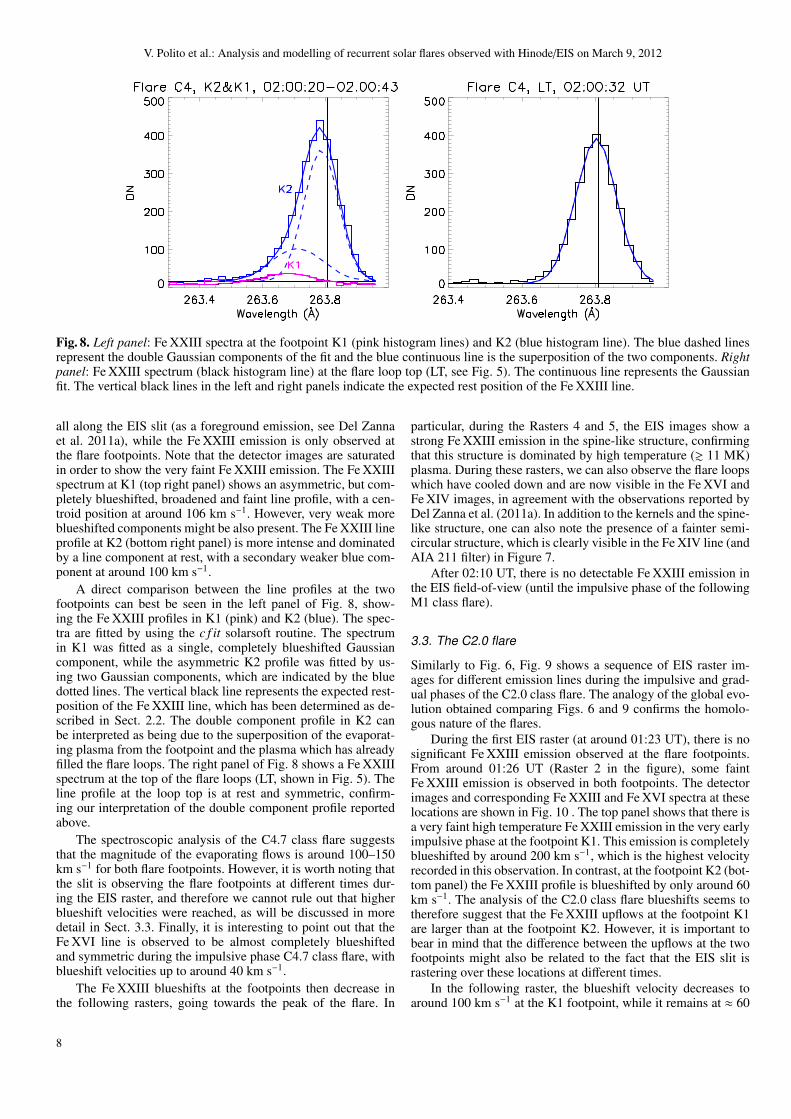
Fig. 8. Left panel: Fe XXIII spectra at the footpoint K1 (pink histogram lines) and K2 (blue histogram line). The blue dashed linesrepresent the double Gaussian components of the fit and the blue continuous line is the superposition of the two components. Rightpanel: Fe XXIII spectrum (black histogram line) at the flare loop top (LT, see Fig. 5). The continuous line represents the Gaussianfit. The vertical black lines in the left and right panels indicate the expected rest position of the Fe XXIII line.

all along the EIS slit (as a foreground emission, see Del Zannaet al. 2011a), while the Fe XXIII emission is only observed atthe flare footpoints. Note that the detector images are saturatedin order to show the very faint Fe XXIII emission. The Fe XXIIIspectrum at K1 (top right panel) shows an asymmetric, but com-pletely blueshifted, broadened and faint line profile, with a cen-troid position at around 106 km s−1. However, very weak moreblueshifted components might be also present. The Fe XXIII lineprofile at K2 (bottom right panel) is more intense and dominatedby a line component at rest, with a secondary weaker blue com-ponent at around 100 km s−1.

A direct comparison between the line profiles at the twofootpoints can best be seen in the left panel of Fig. 8, show-ing the Fe XXIII profiles in K1 (pink) and K2 (blue). The spec-tra are fitted by using the c f it solarsoft routine. The spectrumin K1 was fitted as a single, completely blueshifted Gaussiancomponent, while the asymmetric K2 profile was fitted by us-ing two Gaussian components, which are indicated by the bluedotted lines. The vertical black line represents the expected rest-position of the Fe XXIII line, which has been determined as de-scribed in Sect. 2.2. The double component profile in K2 canbe interpreted as being due to the superposition of the evaporat-ing plasma from the footpoint and the plasma which has alreadyfilled the flare loops. The right panel of Fig. 8 shows a Fe XXIIIspectrum at the top of the flare loops (LT, shown in Fig. 5). Theline profile at the loop top is at rest and symmetric, confirm-ing our interpretation of the double component profile reportedabove.

The spectroscopic analysis of the C4.7 class flare suggeststhat the magnitude of the evaporating flows is around 100–150km s−1 for both flare footpoints. However, it is worth noting thatthe slit is observing the flare footpoints at different times dur-ing the EIS raster, and therefore we cannot rule out that higherblueshift velocities were reached, as will be discussed in moredetail in Sect. 3.3. Finally, it is interesting to point out that theFe XVI line is observed to be almost completely blueshiftedand symmetric during the impulsive phase C4.7 class flare, withblueshift velocities up to around 40 km s−1.

The Fe XXIII blueshifts at the footpoints then decrease inthe following rasters, going towards the peak of the flare. In

particular, during the Rasters 4 and 5, the EIS images show astrong Fe XXIII emission in the spine-like structure, confirmingthat this structure is dominated by high temperature (& 11 MK)plasma. During these rasters, we can also observe the flare loopswhich have cooled down and are now visible in the Fe XVI andFe XIV images, in agreement with the observations reported byDel Zanna et al. (2011a). In addition to the kernels and the spine-like structure, one can also note the presence of a fainter semi-circular structure, which is clearly visible in the Fe XIV line (andAIA 211 filter) in Figure 7.

After 02:10 UT, there is no detectable Fe XXIII emission inthe EIS field-of-view (until the impulsive phase of the followingM1 class flare).

3.3. The C2.0 flare

Similarly to Fig. 6, Fig. 9 shows a sequence of EIS raster im-ages for different emission lines during the impulsive and grad-ual phases of the C2.0 class flare. The analogy of the global evo-lution obtained comparing Figs. 6 and 9 confirms the homolo-gous nature of the flares.

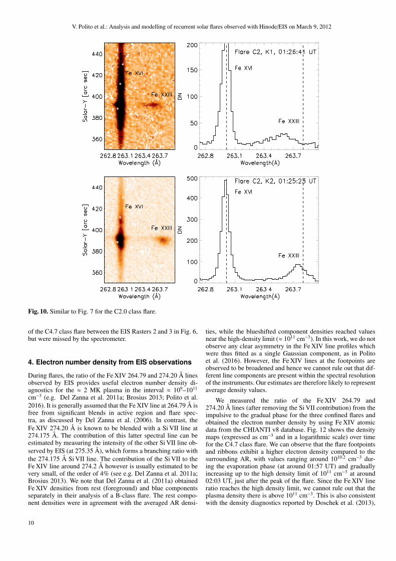
During the first EIS raster (at around 01:23 UT), there is nosignificant Fe XXIII emission observed at the flare footpoints.From around 01:26 UT (Raster 2 in the figure), some faintFe XXIII emission is observed in both footpoints. The detectorimages and corresponding Fe XXIII and Fe XVI spectra at theselocations are shown in Fig. 10 . The top panel shows that there isa very faint high temperature Fe XXIII emission in the very earlyimpulsive phase at the footpoint K1. This emission is completelyblueshifted by around 200 km s−1, which is the highest velocityrecorded in this observation. In contrast, at the footpoint K2 (bot-tom panel) the Fe XXIII profile is blueshifted by only around 60km s−1. The analysis of the C2.0 class flare blueshifts seems totherefore suggest that the Fe XXIII upflows at the footpoint K1are larger than at the footpoint K2. However, it is important tobear in mind that the difference between the upflows at the twofootpoints might also be related to the fact that the EIS slit israstering over these locations at different times.

In the following raster, the blueshift velocity decreases toaround 100 km s−1 at the K1 footpoint, while it remains at ≈ 60

8


Table 3. Maximum Fe XXIII and Fe XVI upflow velocities during the recurrent flares.

Flare Fe XXIII vel Fe XVI vel(km s−1) (km s−1)

K1 K2 K1 K2

C2.0 202 ± 14 60 ± 7 76* 12± 5C4.7 146 ± 10 110* 43 ± 5 39 ± 5

M1.8 (Doschek et al. 2013) 150–170 40–60

Notes. The values followed by an asterisk (∗) represent the velocity of the most blueshifted component when a double Gaussian fit was performed

Fig. 9. Similar to Fig. 6 for the C2.0 class flare

km s−1 at the footpoint K2. There are then no significant upflowsin the Fe XXIII line after about 01:30 UT and the Fe XXIII emis-sion is not visible after ≈ 01:36 UT. The strongest blueshift in theFe XVI line is also observed at the footpoint K1, as shown in thespectrum in Fig. 11. This is the only case we observed wherethe Fe XVI line profile shows a significant asymmetry. The linewas fitted with two Gaussian components (blue dotted lines), themost blueshifted one showing an upflow velocity of ≈ 76 km s−1.

The semi-circular feature observed in the C4.7 flare is alsoclearly visible here, especially in the Fe XIV line. Such a struc-ture, together with the spine-like brightening discussed above,is suggestive of a circular ribbon flare that is usually generatedby reconnection at a null point of the magnetic field at coronalheights, see e.g. Masson et al. (2009), Reid et al. (2012), Sunet al. (2013) and references therein. However, the confirmationof the presence of such a topological feature and its role in thehomologous nature of the flares studied requires more informa-

tion on the underlying magnetic field (for further discussion seeSect. 6).

From a comparison of the blueshifts in the two C-class flares,it seems that higher velocities are reached during the smallerC2.0 class flare. However, we emphasize that the timing of theobservations should also be taken into account. For the C4.7class flare, the area around the footpoint K1 was first observed byEIS at around 01:58 UT, that is ≈ 177 s after the beginning of theflare as measured by the GOES satellite (second column in Tab.1). No significant Fe XXIII is observed there at that time. Duringthe following raster, EIS observes a ≈ 145 km s−1 blueshift atthis footpoint at around 02:00 UT, that is already ≈ 300 s afterthe beginning of the impulsive phase. For the C2.0 class flare,the highest blueshift of ≈ 200 km s−1 is observed at around 220 sinto the impulsive phase of the flare. This suggests that larger up-flows at K1 might have been present during the impulsive phase

9


Fig. 10. Similar to Fig. 7 for the C2.0 class flare.

of the C4.7 class flare between the EIS Rasters 2 and 3 in Fig. 6,but were missed by the spectrometer.

4. Electron number density from EIS observations

During flares, the ratio of the Fe XIV 264.79 and 274.20 Å linesobserved by EIS provides useful electron number density di-agnostics for the ≈ 2 MK plasma in the interval ≈ 109–1011

cm−3 (e.g. Del Zanna et al. 2011a; Brosius 2013; Polito et al.2016). It is generally assumed that the Fe XIV line at 264.79 Å isfree from significant blends in active region and flare spec-tra, as discussed by Del Zanna et al. (2006). In contrast, theFe XIV 274.20 Å is known to be blended with a Si VII line at274.175 Å. The contribution of this latter spectral line can beestimated by measuring the intensity of the other Si VII line ob-served by EIS (at 275.35 Å), which forms a branching ratio withthe 274.175 Å Si VII line. The contribution of the Si VII to theFe XIV line around 274.2 Å however is usually estimated to bevery small, of the order of 4% (see e.g. Del Zanna et al. 2011a;Brosius 2013). We note that Del Zanna et al. (2011a) obtainedFe XIV densities from rest (foreground) and blue componentsseparately in their analysis of a B-class flare. The rest compo-nent densities were in agreement with the averaged AR densi-

ties, while the blueshifted component densities reached valuesnear the high-density limit (≈ 1011 cm−3). In this work, we do notobserve any clear asymmetry in the Fe XIV line profiles whichwere thus fitted as a single Gaussian component, as in Politoet al. (2016). However, the Fe XIV lines at the footpoints areobserved to be broadened and hence we cannot rule out that dif-ferent line components are present within the spectral resolutionof the instruments. Our estimates are therefore likely to representaverage density values.

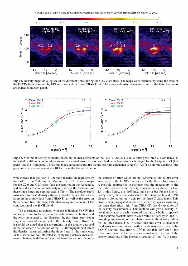
We measured the ratio of the Fe XIV 264.79 and274.20 Å lines (after removing the Si VII contribution) from theimpulsive to the gradual phase for the three confined flares andobtained the electron number density by using Fe XIV atomicdata from the CHIANTI v8 database. Fig. 12 shows the densitymaps (expressed as cm−3 and in a logarithmic scale) over timefor the C4.7 class flare. We can observe that the flare footpointsand ribbons exhibit a higher electron density compared to thesurrounding AR, with values ranging around 1010.2 cm−3 dur-ing the evaporation phase (at around 01:57 UT) and graduallyincreasing up to the high density limit of 1011 cm−3 at around02:03 UT, just after the peak of the flare. Since the Fe XIV lineratio reaches the high density limit, we cannot rule out that theplasma density there is above 1011 cm−3. This is also consistentwith the density diagnostics reported by Doschek et al. (2013),

10


Fig. 12. Density maps (in a log scale) for different times during the C4.7 class flare. The maps were obtained by using the ratio ofthe Fe XIV lines observed by EIS and atomic data from CHIANTI v8. The average density values measured at the flare footpointsare indicated in each panel.

Fig. 13. Maximum density estimates based on the measurements of the Fe XIV 264/274 Å ratio during the three C-class flares, asindicated by different coloured points and associated error bars (as described in the legend on each image) for the footpoints K1 (leftpanel) and K2 (right panel). The solid black curve indicates the theoretical ratio calculated using CHIANTI v8 atomic database. Thegray dotted curves represent a ± 10% error in the theoretical ratio.

who showed that the Fe XIV line ratio reaches the high densitylimit of 1011 cm−3 during the M-class flare. The density mapsfor the C2.0 and C1.0 class flare are reported in the Appendix,and the values of maximum density observed at the footpoints ofthese three flares are summarized in Tab. 4. The absolute errorsassociated to these density estimates should include the uncer-tainty in the atomic data from CHIANTI, as well as the error onthe observed line ratio from EIS, also taking into account of thecontribution of the Si VII blend.

The uncertainty associated with the individual Fe XIV lineintensity is due to the error in the radiometric calibration andthe error associated to the Gaussian fit, this latter error beingvery small, around few percent of the intensity values. However,it should be noted that the uncertainty in the atomic data andin the radiometric calibration of the EIS throughputs will affectthe density measured during the three flares in the same way.In this work, we are interested in comparing density measure-ments obtained in different flares and therefore we consider only

the sources of error which are not systematic, that is, the errorassociated to the Fe XIV line ratios for the three observations.A possible approach is to estimate how the uncertainty in theline ratio can affect the density diagnostics, as shown in Fig.13. In this figure, a ± 10% maximum error bar for the line ra-tios (given by the errors associated to the Gaussian fit and Si VIIblend) is plotted on the y-axis for the three C-class flares. Thiserror is then propagated on the x-axis (density space), assumingthe same theoretical ratio from CHIANTI (solid curve) for allthe density measurements. This method will give a density in-terval associated to each measured line ratio, which is reportedin the curved brackets next to each value of density in Tab. 4,providing an estimate of the relative error in the density valuesfor the three flares. Fig. 13 shows that this error is smaller ifthe density measured is well within the density sensitivity of theFe XIV line ratio (i.e. from ≈ 109.5 to less than 1011 cm−3), butit becomes larger if the density measured is at the edge of thedensity sensitivity of the line ratio (around 1011 cm−3). In partic-

11


Fig. 11. Fe XVI spectrum at the K1 footpoint during the impul-sive phase of the C2.0 class flare. The line profile is asymmetricand has been fitted with two Gaussian components, indicated bythe blue dashed lines.

ular, in this latter case, only a lower value of uncertainty can beestimated, as the upper limit of the line ratio will be outside thedensity sensitivity limit of the line ratio (but still consistent witha density above 1011 cm−3 considering a 10% uncertainty in theatomic data, gray lines). Within the estimated errors, the maxi-mum electron number densities observed during the C1.0 classflare are lower than the C2.0 and C4.7 flares for both footpointK1 and K2, while these latter flares reach in principle similarvalues of density at the footpoint K2. However, by comparingthe density maps in Figs. 12, A.2 and A.1, one can observe thathigher densities (above 1010 cm−3) are reached in the C4.7 classflare at both footpoints for a longer period of time during theimpulsive and peak phase of the flare (note that the three figureshave the same colour scale).

5. Plasma temperature from AIA observations

Despite the multi-thermal nature of the AIA channels, duringflares the 94 Å and 131 Å AIA channels are dominated by emis-sion from Fe XVIII (formed at ∼ 7 MK) and Fe XXI (formedat ∼ 11 MK) respectively (O’Dwyer et al. 2010; Boerner et al.2014). It has been shown previously that the intensity ratio ofthese bands can be used to provide reliable temperature diag-nostics for the flaring plasma (see e.g. Petkaki et al. 2012; DelZanna & Woods 2013). The AIA filter ratio method relies onthe assumption that the plasma is isothermal and dominated byplasma formed in the temperature sensitivity range of the AIA131 and 94 Å ratio (8–12 MK). This is a sensible assumptionclose to or during the peak of flares. In fact, Figs. 6 and 9 showthat during the peak of the flares the flare loops are dominatedby emission from the Fe XXIII ion (formed at around 10 MK),while no emission is observed at that time from cooler emissionlines (e.g. Fe XVI formed at 3 MK and Fe XIV formed at 2 MK).

In Fig. 14, we show the evolution of the plasma temperaturefor the three C-class flares using the 131 Å and 94 Å filter ra-tio. The AIA images were badly saturated during the peak phaseof the C4.7 and C2.0 class flares and cannot be used for diag-nosing the temperature. The first three panels of Fig. 14 showthe temperature maps for the C4.7, C2.0 and C1.0 class flares,respectively from top to bottom. These maps were calculated

Fig. 14. Temperature maps (in Log scale) of the three C-classflares obtained from the 131 and 94 Å AIA filter ratio two min-utes before the peak time for each flare (C4.7, C2.0 and C1.0)and at the peak of the C1.0 flare. The intensity contours of the131 Å channel are overplotted in each panel.

2 minutes and 3 s before the peak of each flare, which is theclosest time to their respective peaks where the AIA images foreach of the three flares are not saturated. The bottom panel showsthe temperature during the peak of the smallest C1.0 flare, werethe AIA images were not significantly saturated. The first three

12


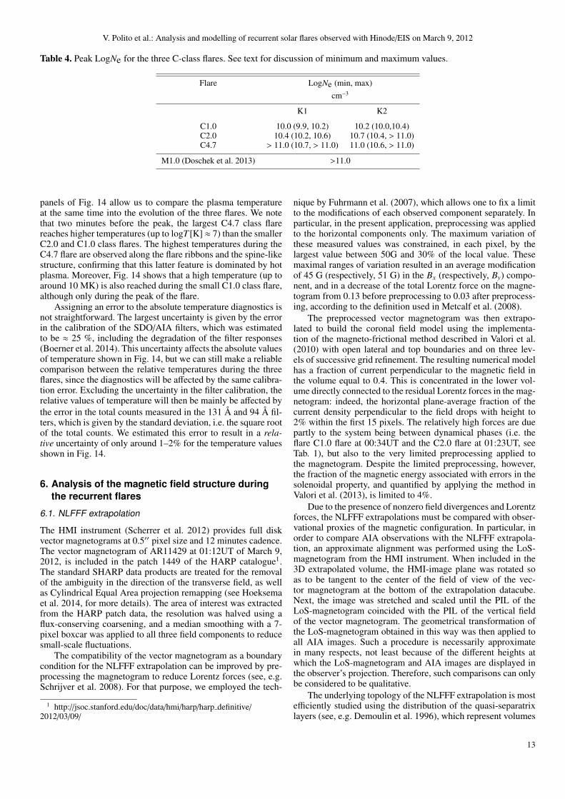
Table 4. Peak LogNe for the three C-class flares. See text for discussion of minimum and maximum values.

Flare LogNe (min, max)cm−3

K1 K2

C1.0 10.0 (9.9, 10.2) 10.2 (10.0,10.4)C2.0 10.4 (10.2, 10.6) 10.7 (10.4, > 11.0)C4.7 > 11.0 (10.7, > 11.0) 11.0 (10.6, > 11.0)

M1.0 (Doschek et al. 2013) >11.0

panels of Fig. 14 allow us to compare the plasma temperatureat the same time into the evolution of the three flares. We notethat two minutes before the peak, the largest C4.7 class flarereaches higher temperatures (up to logT [K] ≈ 7) than the smallerC2.0 and C1.0 class flares. The highest temperatures during theC4.7 flare are observed along the flare ribbons and the spine-likestructure, confirming that this latter feature is dominated by hotplasma. Moreover, Fig. 14 shows that a high temperature (up toaround 10 MK) is also reached during the small C1.0 class flare,although only during the peak of the flare.

Assigning an error to the absolute temperature diagnostics isnot straightforward. The largest uncertainty is given by the errorin the calibration of the SDO/AIA filters, which was estimatedto be ≈ 25 %, including the degradation of the filter responses(Boerner et al. 2014). This uncertainty affects the absolute valuesof temperature shown in Fig. 14, but we can still make a reliablecomparison between the relative temperatures during the threeflares, since the diagnostics will be affected by the same calibra-tion error. Excluding the uncertainty in the filter calibration, therelative values of temperature will then be mainly be affected bythe error in the total counts measured in the 131 Å and 94 Å fil-ters, which is given by the standard deviation, i.e. the square rootof the total counts. We estimated this error to result in a rela-tive uncertainty of only around 1–2% for the temperature valuesshown in Fig. 14.

6. Analysis of the magnetic field structure duringthe recurrent flares

6.1. NLFFF extrapolation

The HMI instrument (Scherrer et al. 2012) provides full diskvector magnetograms at 0.5′′ pixel size and 12 minutes cadence.The vector magnetogram of AR11429 at 01:12UT of March 9,2012, is included in the patch 1449 of the HARP catalogue1.The standard SHARP data products are treated for the removalof the ambiguity in the direction of the transverse field, as wellas Cylindrical Equal Area projection remapping (see Hoeksemaet al. 2014, for more details). The area of interest was extractedfrom the HARP patch data, the resolution was halved using aflux-conserving coarsening, and a median smoothing with a 7-pixel boxcar was applied to all three field components to reducesmall-scale fluctuations.

The compatibility of the vector magnetogram as a boundarycondition for the NLFFF extrapolation can be improved by pre-processing the magnetogram to reduce Lorentz forces (see, e.g.Schrijver et al. 2008). For that purpose, we employed the tech-

1 http://jsoc.stanford.edu/doc/data/hmi/harp/harp definitive/2012/03/09/

nique by Fuhrmann et al. (2007), which allows one to fix a limitto the modifications of each observed component separately. Inparticular, in the present application, preprocessing was appliedto the horizontal components only. The maximum variation ofthese measured values was constrained, in each pixel, by thelargest value between 50G and 30% of the local value. Thesemaximal ranges of variation resulted in an average modificationof 45 G (respectively, 51 G) in the Bx (respectively, By) compo-nent, and in a decrease of the total Lorentz force on the magne-togram from 0.13 before preprocessing to 0.03 after preprocess-ing, according to the definition used in Metcalf et al. (2008).

The preprocessed vector magnetogram was then extrapo-lated to build the coronal field model using the implementa-tion of the magneto-frictional method described in Valori et al.(2010) with open lateral and top boundaries and on three lev-els of successive grid refinement. The resulting numerical modelhas a fraction of current perpendicular to the magnetic field inthe volume equal to 0.4. This is concentrated in the lower vol-ume directly connected to the residual Lorentz forces in the mag-netogram: indeed, the horizontal plane-average fraction of thecurrent density perpendicular to the field drops with height to2% within the first 15 pixels. The relatively high forces are duepartly to the system being between dynamical phases (i.e. theflare C1.0 flare at 00:34UT and the C2.0 flare at 01:23UT, seeTab. 1), but also to the very limited preprocessing applied tothe magnetogram. Despite the limited preprocessing, however,the fraction of the magnetic energy associated with errors in thesolenoidal property, and quantified by applying the method inValori et al. (2013), is limited to 4%.

Due to the presence of nonzero field divergences and Lorentzforces, the NLFFF extrapolations must be compared with obser-vational proxies of the magnetic configuration. In particular, inorder to compare AIA observations with the NLFFF extrapola-tion, an approximate alignment was performed using the LoS-magnetogram from the HMI instrument. When included in the3D extrapolated volume, the HMI-image plane was rotated soas to be tangent to the center of the field of view of the vec-tor magnetogram at the bottom of the extrapolation datacube.Next, the image was stretched and scaled until the PIL of theLoS-magnetogram coincided with the PIL of the vertical fieldof the vector magnetogram. The geometrical transformation ofthe LoS-magnetogram obtained in this way was then applied toall AIA images. Such a procedure is necessarily approximatein many respects, not least because of the different heights atwhich the LoS-magnetogram and AIA images are displayed inthe observer’s projection. Therefore, such comparisons can onlybe considered to be qualitative.

The underlying topology of the NLFFF extrapolation is mostefficiently studied using the distribution of the quasi-separatrixlayers (see, e.g. Demoulin et al. 1996), which represent volumes

13


of sharp gradients in the field line connectivity. The connec-tivity gradient is quantified by the squashing degree Q (Titovet al. 2002), and is computed here using the method in Pariat& Demoulin (2012). In the photospheric Q-map obtained in thisway, high values of Q correspond to separations between differ-ent areas of connectivity.

Fig. 15. Comparison between NLFFF extrapolation andAIA 171 Å image from the AIA viewpoint, at around 01:12 UT.Top: AIA 171 Å image. Middle: NLFFF extrapolation, wheredifferent colors represent different sections of the flux rope.Bottom: Overlay of the AIA 171 Å image and the same fieldlines as in the middle panel.

6.2. Magnetic field analysis

By comparing some selected field lines from the extrapolationwith simultaneous (at ≈ 01:12UT) EUV images from AIA, onecan readily recognize the elongated filament corresponding tothe sheared and twisted flux system along the PIL (see Fig. 15).

Note that the AIA images and the line-of-sight magnetogramfrom SDO/HMI in Fig. 15 are on the (observer) image plane,whereas the vector magnetogram used for the NLFFF extrapola-tion was re-mapped to a Cartesian grid using a CEA projection(see Sect. 6.1). A careful comparison between the middle panelof Fig. 15 and the online AIA Movies 1 and 2 also shows a goodmatch between individual dark strands forming the filament, andindividual sections of the flux rope/sheared structure above thePIL in the NLFFF extrapolation (for instance, the brown south-ern field lines, or the core group of red/violet/blue field lines inFig. 15). In addition, the elongated spine-like structure in thecore, which is already recognizable at this time in the top panelof Fig. 15, has a good correspondence with the spine-like bluefield lines bundle in the extrapolation (see below for the identi-fication of the associated blue fan-like field lines at its easternend). Such details corroborate the quality of the extrapolationdespite the limitations discussed in Sect. 6.1.

Fig. 16. Comparison between the AIA 131 Å image at around01:12 UT, zoom on the ribbon region (top), and selected fieldlines from the NLFFF extrapolation (bottom). The color codingin the latter represents the magnetic field strength.

The magnetic helicity of the NLFFF extrapolation, computedfollowing the method in Valori et al. (2012), is −2.7 × 1043Mx2

(corresponding to 0.05 in units of flux squared). Estimations ofthe helicity of the same active region (but for 24 hours before)were performed by Patsourakos et al. (2016b) using three dif-ferent methods, with values ranging from -0.4×1043 Mx2 to -3.3 ×1043 Mx2. The value obtained with a NLFFF extrapolationcomparable with ours (Chintzoglou et al. 2015b) is -0.8 ×1043

Mx2, which is consistent with our value considering the timespan between the two extrapolations.

The free energy, estimated as in Valori et al. (2013), is 27.4%of the total magnetic energy, which is a value almost 7 timeslarger than the error associated with a violation of the solenoidalproperty in the field. Therefore, the extrapolation shows beyond

14


doubt that the AR under study had significantly high values ofboth free energy and helicity, and was thus in a non-potentialstate. Next, we can use the NLFFF extrapolation at 01:12UT to

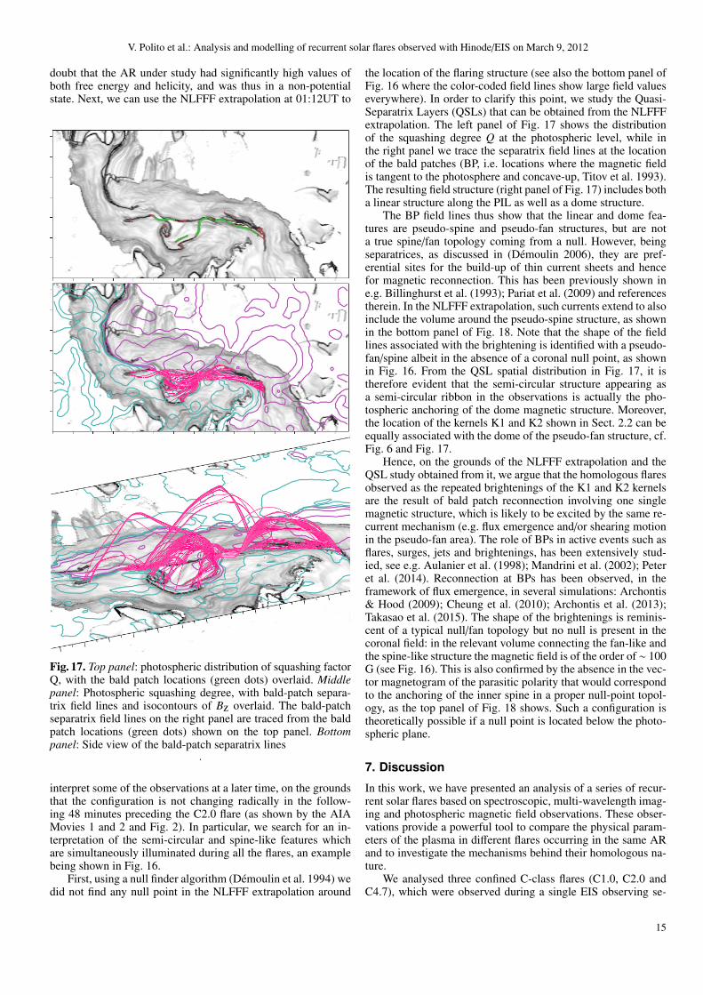
Fig. 17. Top panel: photospheric distribution of squashing factorQ, with the bald patch locations (green dots) overlaid. Middlepanel: Photospheric squashing degree, with bald-patch separa-trix field lines and isocontours of Bz overlaid. The bald-patchseparatrix field lines on the right panel are traced from the baldpatch locations (green dots) shown on the top panel. Bottompanel: Side view of the bald-patch separatrix lines

.

interpret some of the observations at a later time, on the groundsthat the configuration is not changing radically in the follow-ing 48 minutes preceding the C2.0 flare (as shown by the AIAMovies 1 and 2 and Fig. 2). In particular, we search for an in-terpretation of the semi-circular and spine-like features whichare simultaneously illuminated during all the flares, an examplebeing shown in Fig. 16.

First, using a null finder algorithm (Demoulin et al. 1994) wedid not find any null point in the NLFFF extrapolation around

the location of the flaring structure (see also the bottom panel ofFig. 16 where the color-coded field lines show large field valueseverywhere). In order to clarify this point, we study the Quasi-Separatrix Layers (QSLs) that can be obtained from the NLFFFextrapolation. The left panel of Fig. 17 shows the distributionof the squashing degree Q at the photospheric level, while inthe right panel we trace the separatrix field lines at the locationof the bald patches (BP, i.e. locations where the magnetic fieldis tangent to the photosphere and concave-up, Titov et al. 1993).The resulting field structure (right panel of Fig. 17) includes botha linear structure along the PIL as well as a dome structure.

The BP field lines thus show that the linear and dome fea-tures are pseudo-spine and pseudo-fan structures, but are nota true spine/fan topology coming from a null. However, beingseparatrices, as discussed in (Demoulin 2006), they are pref-erential sites for the build-up of thin current sheets and hencefor magnetic reconnection. This has been previously shown ine.g. Billinghurst et al. (1993); Pariat et al. (2009) and referencestherein. In the NLFFF extrapolation, such currents extend to alsoinclude the volume around the pseudo-spine structure, as shownin the bottom panel of Fig. 18. Note that the shape of the fieldlines associated with the brightening is identified with a pseudo-fan/spine albeit in the absence of a coronal null point, as shownin Fig. 16. From the QSL spatial distribution in Fig. 17, it istherefore evident that the semi-circular structure appearing asa semi-circular ribbon in the observations is actually the pho-tospheric anchoring of the dome magnetic structure. Moreover,the location of the kernels K1 and K2 shown in Sect. 2.2 can beequally associated with the dome of the pseudo-fan structure, cf.Fig. 6 and Fig. 17.

Hence, on the grounds of the NLFFF extrapolation and theQSL study obtained from it, we argue that the homologous flaresobserved as the repeated brightenings of the K1 and K2 kernelsare the result of bald patch reconnection involving one singlemagnetic structure, which is likely to be excited by the same re-current mechanism (e.g. flux emergence and/or shearing motionin the pseudo-fan area). The role of BPs in active events such asflares, surges, jets and brightenings, has been extensively stud-ied, see e.g. Aulanier et al. (1998); Mandrini et al. (2002); Peteret al. (2014). Reconnection at BPs has been observed, in theframework of flux emergence, in several simulations: Archontis& Hood (2009); Cheung et al. (2010); Archontis et al. (2013);Takasao et al. (2015). The shape of the brightenings is reminis-cent of a typical null/fan topology but no null is present in thecoronal field: in the relevant volume connecting the fan-like andthe spine-like structure the magnetic field is of the order of ∼ 100G (see Fig. 16). This is also confirmed by the absence in the vec-tor magnetogram of the parasitic polarity that would correspondto the anchoring of the inner spine in a proper null-point topol-ogy, as the top panel of Fig. 18 shows. Such a configuration istheoretically possible if a null point is located below the photo-spheric plane.

7. Discussion

In this work, we have presented an analysis of a series of recur-rent solar flares based on spectroscopic, multi-wavelength imag-ing and photospheric magnetic field observations. These obser-vations provide a powerful tool to compare the physical param-eters of the plasma in different flares occurring in the same ARand to investigate the mechanisms behind their homologous na-ture.

We analysed three confined C-class flares (C1.0, C2.0 andC4.7), which were observed during a single EIS observing se-

15


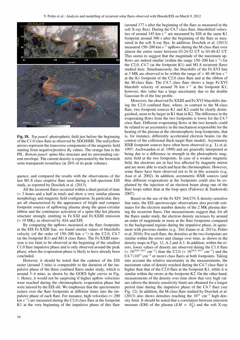
Fig. 18. Top panel: photospheric field just before the beginningof the C1.0 class flare as observed by SDO/HMI. The red/yellowarrows represent the transverse components of the magnetic fieldstarting from negative/positive Bz values. The orange line is thePIL. Bottom panel: spine-like structure and its surrounding cur-rent envelope. The current density is represented by the brownishsemi-transparent isosurface (at 26% of its peak volume).

quence, and compared the results with the observations of thelast M1.8 class eruptive flare seen during a full-spectrum EISstudy, as reported by Doschek et al. (2013).

All the recurrent flares occurred within a short period of time(≈ 3 hours and a half in total) and show a very similar plasmamorphology and magnetic field configuration. In particular, theyare all characterized by the appearance of bright and compactfootpoint sources of upflowing plasma along the quasi-circularribbon and the continuous activation of a spine-like hot plasmastructure strongly emitting in Fe XXI and Fe XXIII emission(≈ 10 MK), as observed by AIA and EIS.

By comparing the upflows measured at the flare footpointsin the EIS Fe XXIII line, we found similar values of blueshiftsvelocity (of the order of 150–200 km s−1) in the C2.0, C4.7(at the footpoint K1) and M1.8 class flares. The Fe XXIII emis-sion is too faint to be observed at the beginning of the smallestC1.0 flare impulsive phase and is only observed around the peakphase, when the evaporation phase is likely to have already beenconcluded.

However, it should be noted that the cadence of the EISraster (around 3 min) is comparable to the duration of the im-pulsive phase of the three confined flares under study, which isaround 3–4 mins, as shown by the GOES light curves in Fig.1. Hence, it would not be surprising if higher upflow velocitieswere reached during the chromospheric evaporation phase butwere missed by the EIS slit. We emphasize that the spectrometerrasters over the flare footpoints at different times into the im-pulsive phase of each flare. For instance, high velocities (≈ 200km s−1) are measured during the C2.0 class flare at the footpointK1 at the very beginning of the impulsive phase of this flare

(around 177 s after the beginning of the flare as measured in thesoft X-ray flux). During the C4.7 class flare, blueshifted veloci-ties of around 145 km s−1 are measured by EIS at the same K1footpoint around 300 s after the beginning of the flare as mea-sured in the soft X-ray flux. In addition, Doschek et al. (2013)measured 150–200 km s−1 upflows during the M-class flare overalmost the entire raster between 03:24:52 UT to 03:40:42 UT.This seems to suggest that the magnitude of the maximum up-flows are indeed similar (within the range 150–200 km s−1) forthe C2.0, C4.7 (at the footpoint K1) and M1.8 recurrent flaresstudied here. Simultaneously, the blueshifts of the Fe XVI lineat 3 MK are observed to be within the range of ≈ 40–60 km s−1

at the K1 footpoint of the C2.0 class flare and at the ribbon ofthe M-class flare. The C4.7 class flare shows a large Fe XVIblueshift velocity of around 76 km s−1 at the footpoint K1;however, this value has a large uncertainty due to the doubleGaussian fit of the line profile.

Moreover, the observed Fe XXIII and Fe XVI blueshifts dur-ing the C2.0 confined flare, where, in contrast to the M-classflare, two footpoint sources K1 and K2 could be clearly distin-guished, seem to be larger in K1 than in K2. The difference in theevaporating flows from the two footpoints is lower for the C4.7class flare. Different evaporating flows at the two kernels couldbe related to an asymmetry in the mechanism responsible for theheating of the plasma at the chromospheric loop footpoints, thatis, for instance, differently accelerated electron beams (in thecontext of the collisional thick-target flare model). AsymmetricHXR footpoint sources have often been observed (e.g. Li et al.1997; Aschwanden et al. 1999) and are generally interpreted asbeing due to a difference in strength in the photospheric mag-netic field at the two footpoints. In case of a weaker magneticfield, the electrons are in fact less affected by magnetic mirrorand are more able to reach and heat the chromosphere. However,some flares have been observed not to fit in this scenario (e.g.Asai et al. 2002). In addition, asymmetric HXR sources (andthus different evaporation) at the footpoints could also be ex-plained by the injection of an electron beam along one of theflare loops rather than at the loop apex (Falewicz & Siarkowski2007).

Based on the use of the Fe XIV 264/274 Å density-sensitiveline ratio, the EIS spectroscopic observations also provide esti-mates for the electron number density of the 2 MK plasma dur-ing the recurrent flares. Our measurements suggest that, for allthe flares under study, the electron density increases by aroundan order of magnitude or more at the flare footpoints comparedto the background regions during the impulsive phase, in agree-ment with previous studies (e.g. Del Zanna et al. 2011a; Politoet al. 2016). For each flare, the densities at the two footpoints aresimilar within the errors and change over time, as shown in thedensity maps in Figs. 12, A.2 and A.1. In addition, within the er-rors, lower values of density are observed during the C1.0 flare(≈ 1010.0−10.2 cm−3) than the C2.0 (≈ 1010.4−10.7 cm−3) and theC4.7 (1011 cm−3 or more) class flares at both footpoints. Takinginto account the relative uncertainty in the measurements, themaximum value of density reached during the C4.7 class flare ishigher than that of the C2.0 flare at the footpoint K1, while it issimilar within the errors at the footpoint K2. On the other hand,measurements of the density over time show that very high val-ues (above the density sensitivity limit) are obtained for a longerperiod time during the impulsive phase of the C4.7 flare (seeFig. 12). In addition, the M-class flare studied by Doschek et al.(2013) also shows densities reaching the 1011 cm−3 high den-sity limit. It should be noted that a correlation between emissionmeasure (EM) of the plasma (EM ∝ N2

e) and the soft X-ray

16


flux was also observed by previous authors, e.g. Feldman et al.(1996), Battaglia et al. (2005).

Given that similar velocities are observed during flares ofdifferent size, an increase in the electron number density withlarger peak soft X-ray flux would indeed be expected in orderto satisfy conservation of momentum of the plasma evaporatingfrom the flare kernels and filling the flare loops (in the context ofthe standard model of flares). For instance, assuming the samesize for the C2.0 and C4.7 flare footpoint sources (as observedwithin the EIS spatial resolution), the ratio between the peaksoft X-ray energy of the two flares is around a factor of ≈ 2.3(4.7/2.0) from the GOES measurements. This value is consistentwith the ratio of density values measured during the two flares(i.e. 1011/1010.6 ≈ 2.5).

Finally, the temperature diagnostics based on the AIA131/94 Å line ratio show that high temperature plasma (≈ 10MK) is observed at the flare footpoints and spine-like struc-ture, as also confirmed by the spectroscopic measurements in theFe XXIII line with EIS. In addition, by comparing the tempera-ture diagnostics during the three confined flares, we observe thatslightly higher temperatures (around 10 % higher with a relativeuncertainty of 1–2%) are reached a few minutes before the peakof the C4.7 flare than those of the other two flares. It is empha-sized that an increase in the electron temperature with peak softX-ray flux of the flare is in agreement with previous results bye.g. Feldman et al. (1996). However, since the AIA images arebadly saturated during the peak of the C2.0 and C4.7 class flares,reliable temperature measurements and conclusive comparisonscannot be obtained.

In order to understand the context of the observed eventsand investigate the mechanism responsible for the homologousflares, we performed a NLFFF extrapolation of the 3D mag-netic field configuration in the corona. The NLFFF extrapolationcatches the global topology and provides a good agreement withthe location of the quasi-circular ribbon and the 10 MK spine-like structure observed in AIA 131 Å. The extrapolation pro-vides the magnetic field context that is sufficient to interpretand explain the locations of all brightenings involved in the(non-eruptive) flares (kernels, spine, semi-circular brightenings)which have been studied.

The semi-circular ribbon shape is similar to those created bythe presence of a coronal null point, plus an associated spine-like structure connected to the circular one. However, there isno coronal null point, not just because it is absent in the NLFFFextrapolation, but because the observed photospheric field doesnot show the parasitic polarity necessary for its existence in thecorona. Instead, bald patch reconnection activates a magneticstructure consisting of a pseudo-fan and pseudo-spine. Such aconfiguration is conceivable as the geometrical prolongation inthe corona of a sub-photospheric null point structure. On thebasis of the NLFFF and the QSL study, we argue that the ho-mologous flares were all generated by a repetition of the sameprocess, namely bald patch reconnection.

We interpret the time evolution of the GOES fluxes in Fig.1 and the temperature distribution estimations in Fig. 14 as in-dications of a progressive increase in energy of the events con-sidered. Within the validity of the linear force-free theory, Valoriet al. (2015) derives the relation

∆Efree '1

4πHm∆α (1)

that relates the drop in free energy ∆Efree due to a flare to thechange in the force-free parameter ∆α and the relative magnetic

helicity of the whole active region, Hm. The considered homolo-gous flares are repetitions of roughly the same reconnection pro-cess, hence, in the spirit of the linear theory, we can represent thechange in connectivity producing them as a similar change ∆αin the linear parameter characterizing the field. Since the activeregion is in an emerging phase with increasing energy (and helic-ity) over several days (Dhakal & Zhang 2016), then Eq. 1 showsthat the same (small) drop in ∆ α generates flares that are higherand higher in energy, due to the increased accumulated helicityin time. In this sense, Eq. 1 provides a simple explanation whyhomologous flares often show a progressive increase in energy,as it does for the case under examination, see Fig. 1. However,this simple explanation is based on the linear theory, and inheritsits limited range of applicability, especially when dealing withfully non-linear configurations, as in the case treated here.

The EIS observations in this work, coupled with the mod-elling of the magnetic field structure based on the NLFFF extrap-olation, provide important information on the physical conditionof the plasma and the reconnection process during the recurrentflares. In particular, the plasma parameters obtained by the anal-ysis of the EIS spectra provide constraints for hydrodynamicalmodels using different values of total energy inputs (for eachflare) and based on different heating mechanisms, such as elec-tron beams or conduction fronts, assuming different time profilesand geometries for the heating injection.

In order to confirm the results of the comparative analysispresented in this work, future spectroscopic studies of recurrentflares would need higher temporal cadence observations at thesame footpoint source. This could best be achieved with an EISsit-and-stare rather than a raster observing mode. On the otherhand, raster observations offer the advantage of observing bothfootpoint sources, but higher cadence than the one used in thisstudy would still be desirable.

Acknowledgements. VP acknowledges support from the Isaac NewtonStudentship and the Cambridge Trust. GDZ and HEM acknowledge supportfrom the STFC and the RS Newton Alumni Programme. J.D. acknowledgessupport from the Grant Agency of the Czech Republic (GA CR), projects No.P209/12/1652, and 16-17586S. V.P., G.D.Z., H.E.M., and J.D. acknowledgesupport from the Royal Society via the Newton Alumni programme. GVacknowledges the support of the Leverhulme Trust Research Project Grant2014-051.

Hinode is a Japanese mission developed and launched by ISAS/JAXA, withNAOJ as domestic partner and NASA and STFC (UK) as international partners.It is operated by these agencies in co-operation with ESA and NSC (Norway).AIA and HMI data are courtesy of NASA/SDO and their respective scienceteams. CHIANTI is a collaborative project involving researchers at the universi-ties of Cambridge (UK), George Mason and Michigan (USA).

Appendix A: Density diagnostics in the C2.0 andC1.0 class flares

ReferencesAntonucci, E., Gabriel, A. H., Acton, L. W., et al. 1982, Sol. Phys., 78, 107Archontis, V. & Hood, A. W. 2009, A&A, 508, 1469Archontis, V., Hood, A. W., & Tsinganos, K. 2013, ApJ, 778, 42Asai, A., Masuda, S., Yokoyama, T., et al. 2002, ApJ, 578, L91Aschwanden, M. J., Fletcher, L., Sakao, T., Kosugi, T., & Hudson, H. 1999, ApJ,

517, 977Aulanier, G., Demoulin, P., Schmieder, B., Fang, C., & Tang, Y. H. 1998,

Sol. Phys., 183, 369Aulanier, G., Janvier, M., & Schmieder, B. 2012, A&A, 543, A110Battaglia, M., Grigis, P. C., & Benz, A. O. 2005, A&A, 439, 737Battaglia, M., Kleint, L., Krucker, S., & Graham, D. 2015, ApJ, 813, 113Billinghurst, M. N., Craig, I. J. D., & Sneyd, A. D. 1993, A&A, 279, 589Boerner, P., Edwards, C., Lemen, J., et al. 2012, Sol. Phys., 275, 41Boerner, P. F., Testa, P., Warren, H., Weber, M. A., & Schrijver, C. J. 2014,

Sol. Phys., 289, 2377

17


Fig. A.1. Density maps (in log scale) for different times during the C1.0 class flare. See caption of Fig. 12 for more details.

Fig. A.2. Density maps (in log scale) for different times during the C2.0 class flare. See caption of Fig. 12 for more details.

Brosius, J. W. 2003, ApJ, 586, 1417Brosius, J. W. 2013, ApJ, 762, 133Carmichael, H. 1964, NASA Special Publication, 50, 451Cheung, M. C. M., Rempel, M., Title, A. M., & Schussler, M. 2010, ApJ, 720,

233Chintzoglou, G., Patsourakos, S., & Vourlidas, A. 2015a, ApJ, 809, 34Chintzoglou, G., Patsourakos, S., & Vourlidas, A. 2015b, ApJ, 809, 34Culhane, J. L., Harra, L. K., James, A. M., et al. 2007, Sol. Phys., 243, 19De Pontieu, B., Title, A. M., Lemen, J. R., et al. 2014, Sol. Phys., 289, 2733Del Zanna, G., Berlicki, A., Schmieder, B., & Mason, H. E. 2006, Sol. Phys.,

234, 95Del Zanna, G., Mitra-Kraev, U., Bradshaw, S. J., Mason, H. E., & Asai, A.

2011a, A&A, 526, A1Del Zanna, G., O’Dwyer, B., & Mason, H. E. 2011b, A&A, 535, A46Del Zanna, G. & Woods, T. N. 2013, A&A, 555, A59Demoulin, P. 2006, Advances in Space Research, 37, 1269Demoulin, P., Henoux, J. C., & Mandrini, C. H. 1994, A&A, 285, 1023Demoulin, P., Henoux, J. C., Priest, E. R., & Mandrini, C. H. 1996, A&A, 308,

643Dhakal, S. K. & Zhang, J. 2016, in AAS/Solar Physics Division Meeting, Vol. 47,

AAS/Solar Physics Division Meeting, 11.02Doschek, G. A., Kreplin, R. W., & Feldman, U. 1979, ApJ, 233, L157Doschek, G. A., Warren, H. P., Dennis, B. R., Reep, J. W., & Caspi, A. 2015,

ApJ, 813, 32Doschek, G. A., Warren, H. P., & Young, P. R. 2013, ApJ, 767, 55Dudık, J., Janvier, M., Aulanier, G., et al. 2014, ApJ, 784, 144Dudık, J., Polito, V., Janvier, M., et al. 2016, ApJ, 823, 41Emslie, G. A. & Alexander, D. 1987, Sol. Phys., 110, 295Falewicz, R. & Siarkowski, M. 2007, A&A, 461, 285

Feldman, U., Doschek, G. A., Behring, W. E., & Phillips, K. J. H. 1996, ApJ,460, 1034

Fuhrmann, M., Seehafer, N., & Valori, G. 2007, A&A, 476, 349Graham, D. R., Hannah, I. G., Fletcher, L., & Milligan, R. O. 2013, ApJ, 767,

83Hannah, I. G., Hudson, H. S., Battaglia, M., et al. 2011, Space Sci. Rev., 159,

263Hao, Q., Guo, Y., Dai, Y., et al. 2012, A&A, 544, L17Harrison, R. A., Sawyer, E. C., Carter, M. K., et al. 1995, Sol. Phys., 162, 233Hirayama, T. 1974, Sol. Phys., 34, 323Hoeksema, J. T., Liu, Y., Hayashi, K., et al. 2014, Sol. Phys., 289, 3483Janvier, M., Aulanier, G., & Demoulin, P. 2015, Sol. Phys., 290, 3425Janvier, M., Aulanier, G., Pariat, E., & Demoulin, P. 2013, A&A, 555, A77Kahler, S. W. 1982, J. Geophys. Res., 87, 3439Kamio, S., Hara, H., Watanabe, T., Fredvik, T., & Hansteen, V. H. 2010,

Sol. Phys., 266, 209Kopp, R. A. & Pneuman, G. W. 1976, Sol. Phys., 50, 85Kouloumvakos, A., Patsourakos, S., Nindos, A., et al. 2016, ApJ, 821, 31Li, J., Metcalf, T. R., Canfield, R. C., Wulser, J.-P., & Kosugi, T. 1997, ApJ, 482,

490Mandrini, C. H., Demoulin, P., Schmieder, B., Deng, Y. Y., & Rudawy, P. 2002,

A&A, 391, 317Masson, S., Pariat, E., Aulanier, G., & Schrijver, C. J. 2009, ApJ, 700, 559Metcalf, T. R., Derosa, M. L., Schrijver, C. J., et al. 2008, Sol. Phys., 247, 269Milligan, R. O. 2015, Sol. Phys., 290, 3399Milligan, R. O., Gallagher, P. T., Mathioudakis, M., et al. 2006, ApJ, 638, L117Nitta, N. V. & Hudson, H. S. 2001, Geophys. Res. Lett., 28, 3801O’Dwyer, B., Del Zanna, G., Mason, H. E., Weber, M. A., & Tripathi, D. 2010,

A&A, 521, A21

18


Pariat, E. & Demoulin, P. 2012, A&A, 541, A78Pariat, E., Masson, S., & Aulanier, G. 2009, ApJ, 701, 1911Patsourakos, S., Georgoulis, M. K., Vourlidas, A., et al. 2016a, ApJ, 817, 14Patsourakos, S., Georgoulis, M. K., Vourlidas, A., et al. 2016b, ApJ, 817, 14Peter, H., Tian, H., Curdt, W., et al. 2014, Science, 346, 1255726Petkaki, P., Del Zanna, G., Mason, H. E., & Bradshaw, S. J. 2012, A&A, 547,

A25Polito, V., Reep, J. W., Reeves, K. K., et al. 2016, ApJ, 816, 89Priest, E. R. & Demoulin, P. 1995, J. Geophys. Res., 100, 23443Reeves, K. K., Warren, H. P., & Forbes, T. G. 2007, ApJ, 668, 1210Reid, H. A. S., Vilmer, N., Aulanier, G., & Pariat, E. 2012, A&A, 547, A52Romano, P., Zuccarello, F., Guglielmino, S. L., et al. 2015, A&A, 582, A55Scherrer, P. H., Schou, J., Bush, R. I., et al. 2012, Sol. Phys., 275, 207Schrijver, C. J., DeRosa, M. L., Metcalf, T., et al. 2008, ApJ, 675, 1637Simoes, P. J. A., Fletcher, L., Hudson, H. S., & Russell, A. J. B. 2013, ApJ, 777,

152Sturrock, P. A. 1968, The Astronomical Journal Supplement, 73, 78Sun, X., Hoeksema, J. T., Liu, Y., et al. 2013, ApJ, 778, 139Syntelis, P., Gontikakis, C., Patsourakos, S., & Tsinganos, K. 2016, A&A, 588,

A16Takasao, S., Fan, Y., Cheung, M. C. M., & Shibata, K. 2015, ApJ, 813, 112Teriaca, L., Falchi, A., Cauzzi, G., et al. 2003, ApJ, 588, 596Titov, V. S., Hornig, G., & Demoulin, P. 2002, Journal of Geophysical Research

(Space Physics), 107, 1164Titov, V. S., Priest, E. R., & Demoulin, P. 1993, A&A, 276, 564Valori, G., Demoulin, P., & Pariat, E. 2012, Sol. Phys., 278, 347Valori, G., Demoulin, P., Pariat, E., & Masson, S. 2013, A&A, 553, A38Valori, G., Kliem, B., Torok, T., & Titov, V. S. 2010, A&A, 519, A44+Valori, G., Romano, P., Malanushenko, A., et al. 2015, Sol. Phys., 290, 491Warren, H. P. & Doschek, G. A. 2005, ApJ, 618, L157Young, P. R., O’Dwyer, B., & Mason, H. E. 2012, ApJ, 744, 14

19

Analysis and modelling of recurrent solar ﬂares observed ... · Analysis and modelling of...

Documents

Transcript of Analysis and modelling of recurrent solar ﬂares observed ... · Analysis and modelling of...