Evaluation of trace-metal and isotopic records as ...
145
University of South Florida Scholar Commons Graduate eses and Dissertations Graduate School July 2018 Evaluation of trace-metal and isotopic records as techniques for tracking lifetime movement paerns in fishes Jennifer E. Granneman University of South Florida, [email protected] Follow this and additional works at: hps://scholarcommons.usf.edu/etd Part of the Other Oceanography and Atmospheric Sciences and Meteorology Commons is Dissertation is brought to you for free and open access by the Graduate School at Scholar Commons. It has been accepted for inclusion in Graduate eses and Dissertations by an authorized administrator of Scholar Commons. For more information, please contact [email protected]. Scholar Commons Citation Granneman, Jennifer E., "Evaluation of trace-metal and isotopic records as techniques for tracking lifetime movement paerns in fishes" (2018). Graduate eses and Dissertations. hps://scholarcommons.usf.edu/etd/7675
Transcript of Evaluation of trace-metal and isotopic records as ...

University of South FloridaScholar Commons
Graduate Theses and Dissertations Graduate School
July 2018
Evaluation of trace-metal and isotopic records astechniques for tracking lifetime movement patternsin fishesJennifer E. GrannemanUniversity of South Florida, [email protected]
Follow this and additional works at: https://scholarcommons.usf.edu/etdPart of the Other Oceanography and Atmospheric Sciences and Meteorology Commons
This Dissertation is brought to you for free and open access by the Graduate School at Scholar Commons. It has been accepted for inclusion inGraduate Theses and Dissertations by an authorized administrator of Scholar Commons. For more information, please [email protected].
Scholar Commons CitationGranneman, Jennifer E., "Evaluation of trace-metal and isotopic records as techniques for tracking lifetime movement patterns infishes" (2018). Graduate Theses and Dissertations.https://scholarcommons.usf.edu/etd/7675

Evaluation of trace-metal and isotopic records as techniques for tracking lifetime movement
patterns in fishes
by
Jennifer E. Granneman
A dissertation submitted in partial fulfillment
of the requirements for the degree of
Doctor of Philosophy
with a concentration in Marine Resource Assessment
College of Marine Science
University of South Florida
Co-Major Professor: Ernst B. Peebles, Ph.D.
Co-Major Professor: Steven A. Murawski, Ph.D.
William F. Patterson, III, Ph.D.
Cameron H. Ainsworth, Ph.D.
David J. Hollander, Ph.D.
Date of Approval:
April 9, 2018
Keywords: otolith microchemistry, eye lens, stable isotopes, trace elements, diet switch, meta-
analysis
Copyright © 2018, Jennifer E. Granneman 2018

Dedication
This work is dedicated to Dr. David Jones for his guidance, patience, and pursuit of the
significant truth.

Acknowledgements
I could not have achieved all I set out to do without the love and support of my family.
My husband is my cornerstone and I am deeply appreciative of all the love, patience, and
guidance he has provided throughout this trial. I would also like to thank my soul sisters and
aunt for their constant empathy; they helped me through the times when I wasn’t sure if it was
worth continuing to pursue this degree. My parents helped to instill the grit I needed to achieve
this goal, and for that I will be eternally thankful.
I must thank my co-advisors, Dr. Ernst Peebles and Dr. Steve Murawski, for their
financial support and mentorship offered to me during my time at USF. I also thank the
members of my dissertation committee - Dr. Cameron Ainsworth, Dr. David Hollander, and Dr.
William Patterson, III - for their feedback on this research. I would especially like to
acknowledge the late Dr. David Jones, my friend and committee member, for his support and
kindness throughout this academic journey.
This research was made possible in part by financial support provided by the William and
Elsie Knight Endowed Fellowship Fund for Marine Science, the Paul Getting Endowed
Memorial Fellowship in Marine Science, the Gulf of Mexico Research Initiative/C-IMAGE I
and II (SA 15-16), the State of Louisiana (S203-4S-2121), and the National Fisheries Institute.

i
Table of Contents
List of Tables iii
List of Figures v
Abstract vii
Chapter 1. Introduction 1
Chapter 2. Associations between metal exposure and lesion formation in offshore Gulf of
Mexico fishes collected after the Deepwater Horizon oil spill 6
2.1 Research Overview 6
2.2 Note to Reader 7
Chapter 3. Otolith microchemistry meta-analysis including the Gulf of Mexico, West
Atlantic, and Caribbean Sea 8
Abstract 8
3.1 Introduction 9
3.2 Methods 14
3.2.1 Trends in Concentrations of the Most Common Elements 16
3.2.2 One-way ANOVAs of Regions and Species 16
3.2.3 Multiple Comparison Tests of Regions and Families 17
3.3 Results 19
3.3.1 Trends in Concentrations of the Most Common Elements 19
3.3.2 One-way ANOVAs of Regions and Species 21
3.3.3 Multiple Comparison Tests of Regions and Families 23
3.3.4 Tests of Ecological Niches 25
3.4 Discussion 26
3.5 Tables 34
3.6 Figures 45
Chapter 4. Fish eye-lens response to an experimental step-change in dietary δ15N 55
Abstract 55
4.1 Introduction 55
4.2 Methods 57
4.2.1 Experimental animals and feed 57
4.2.2 Eye-lens isotope measurements 58
4.2.3 Isotope analysis 59
4.2.4 Lens-age relationship 59
4.2.5 Analysis of isotope data 60

ii
4.3 Results 62
4.4 Discussion 63
4.4.1 The pathway to isotopic conservation 63
4.4.2 Model shape and isotopic lags 66
4.4.3 Isotopic discrimination 69
4.4.4 Conclusions 70
4.5 Tables 72
4.6 Figures 75
Chapter 5. Examination of post-settlement movement patterns of Red Snapper (Lutjanus
campechanus) in the Gulf of Mexico 79
Abstract 79
5.1 Introduction 80
5.2 Methods 84
5.2.1 Regional otolith microchemistry 84
5.2.2 Field collection 84
5.2.3 Eye lens analysis 85
5.2.4 Otolith analysis 85
5.2.5 Statistical Analyses 86
5.3 Results 87
5.4 Discussion 88
5.5 Tables 95
5.6 Figures 99
Chapter 6. Conclusions 102
References 107
Appendix A: Author contributions and copyright permissions 116
Appendix B: Published chapter 117

iii
List of Tables
Table 3.1 Summary of the elements, studies, families, and regions included in the
study listed by species 34
Table 3.2 Average constituent values separated by regions, families, and ecological
niches 39
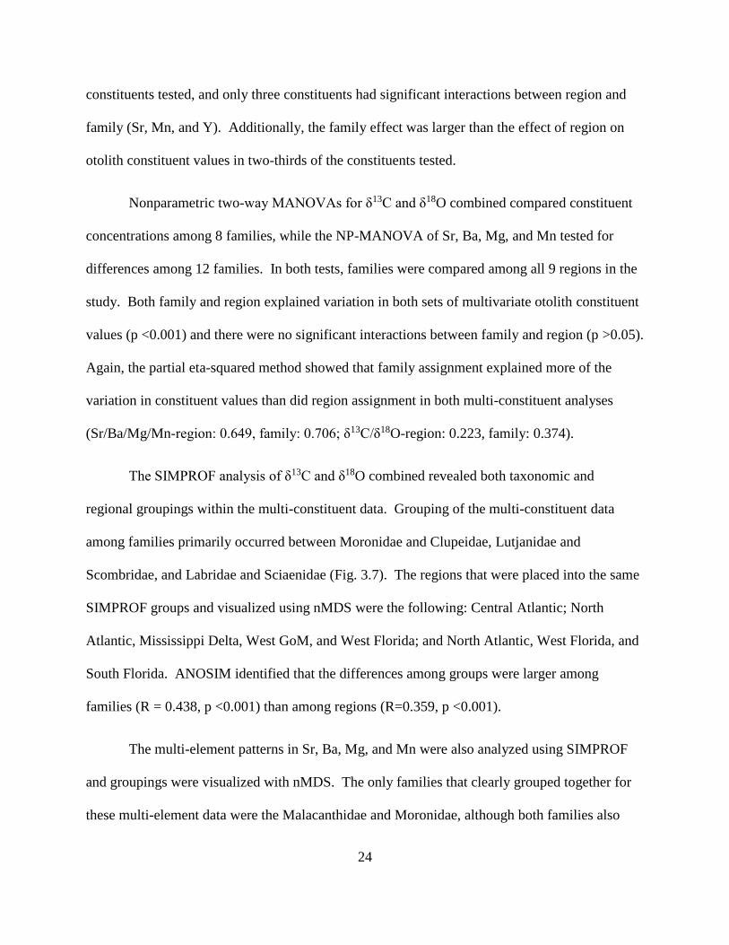
Table 3.3 Average element concentrations for Mg, Mn, Sr, and Ba separated by
migration- and habitat-type 41
Table 3.4 Results of one-way permutation-based ANOVAs to test whether there are
significant differences among species within a region 42
Table 3.5 Results of one-way permutation-based ANOVAs to test whether there are
significant differences across regions for a species 43
Table 3.6 Results of two-way, permutation-based ANOVAs to determine if there is a
significant difference in otolith element concentrations among families and
regions 44
Table 4.1 Feeding schedule of captive red drum 72
Table 4.2 Summary of water quality data during the experiment 72
Table 4.3 Characteristics of each of the red drum individuals at the end of the
experiment 73
Table 4.4 Results of Heady and Moore (3013) regression models for individual red
drum specimens (tissue turnover equation), including change-point lag,
residence time (τ) with standard error (SE), time to 90% tissue turnover
(t90), and model fit, as R2 74
Table 5.1 Reproduced from Patterson 2007 with additional recent studies 95
Table 5.2 Reproduced from Patterson 2007 with additional recent studies 96
Table 5.3 Summary of Red Snapper otolith microchemistry studies used to define
Regional element concentrations 97
Table 5.4 Results of permutation-based regression analyses of otolith element

iv
concentrations and δ15N over the life of each Red Snapper analyzed in
this study 97
Table 5.5 Results of permutation-based regression analyses of otolith element
concentrations over the life of each Red Snapper analyzed in this study 98

v
List of Figures
Figure 3.1 Locations of sample collections from all studies used in this meta-analysis 45
Figure 3.2 Boxplots of δ13C ratios (%, Air) in otoliths shown among regions (a),
families (b), and ecological niches (c). 46
Figure 3.3 Boxplots of δ18O ratios (%, Air) in otoliths shown among regions (a),
families (b), and ecological niches (c) 47
Figure 3.4 Boxplots of element concentrations (ppm) shown among regions for Ba (a),
Mg (b), Mn (c), and Sr (d) 48
Figure 3.5 Boxplots of element concentrations (ppm) shown among ecological niches for
Ba (a), Mg (b), Mn (c), and Sr (d) 49
Figure 3.6 Boxplots of element concentrations (ppm) shown among families for Ba (a),
Mg (b), Mn (c), and Sr (d) 50
Figure 3.7 Non-metric multi-dimensional scaling (nMDS) plot of δ13C and δ18O
otolith concentrations with SIMPROF groupings outlined for regions (a)
and families (b) 51
Figure 3.8 Non-metric multi-dimensional scaling (nMDS) plot of Ba, Mg, Mn, and
Sr otolith concentrations with SIMPROF groupings outlined for regions (a)
and families (b) 52
Figure 3.9 Comparison of effect size of environment, physiology, and niche as
determined using the partial eta-squared method. 53
Figure 3.10 Non-metric multi-dimensional scaling (nMDS) plot of (a) Ba, Mg, Mn, and
Sr and (b) δ13C and δ18O otolith concentrations with SIMPROF groupings
outlined for ecological niches 54
Figure 4.1 Regression describing the change in fish length (SL) with change in eye-
lens diameter (d), where SL = 5.404 + 1.97d2 + 36.98d (n = 145,
R2 = 0.98, p <0.0001) 75
Figure 4.2 Eye-lens δ15N values from 18 red drum raised in captivity from the egg
stage to an age of 201-210 d 76

vi
Figure 4.3 Variation in the δ15N values of fish feed and red drum eye-lens laminae
during time in captivity 77
Figure 4.4 Fit of the Heady and Moore (2013) single-compartment turnover model
Y = b3 – (b3 – b2)(exp[-1(t/b1)]) to measured δ15N, where day 0 was set to
the change points in Figure 4.3a and the regression was applied to data from
all individuals combined 78
Figure 5.1 Boxplots of otolith element concentrations among regions in the GoM for
Red Snapper 99
Figure 5.2 Otolith concentrations of Mg (a), Mn (b), Sr (c), and Ba (d) with each
plotted line representing a different specimen captured in Tampa Bay 100
Figure 5.3 Otolith concentrations of Mg (a), Mn (b), Sr (c), and Ba (d) with each
plotted line representing a different specimen captured at the
Alabama/Mississippi Border 101

vii
Abstract
The focus of this work was on the use of otolith microchemistry and fish eye lens
chemical profiles to measure fish movement and provided indirect support for the use of otolith
microchemistry to examine exposure to crude oil. Chapter 1 provides an introduction to the
applications of otolith microchemistry and eye lens isotopic profiles. In the second chapter,
which examined associations between metal exposure and lesion formation in fishes collected
after the Deepwater Horizon (DWH) oil spill, I did not observe any change in oil-associated
metal concentrations in otoliths coinciding with the timing of the DWH oil spill. This suggests
that either the technique used is not sensitive enough to detect any transient changes that may
have occurred because of exposure to the oil spill or that the fish examined were not exposed to
the oil spill. However, I did find that lesioned fish may have been exposed to a persistent source
of trace-metals in the GoM prior to, during, and after the oil spill, and metal-induced
immunomodulation may have occurred in these fish. These interactions between the
physiological and environmental modulation of otolith element incorporation were explored
further in Chapter 3 in which multiple tests demonstrated that physiology explained more of the
variation in otolith chemical tags than ambient water chemistry. These findings suggest that the
use of otolith microchemistry alone to track fish movement and potential exposure to harmful
metals may be complicated by physiological control of otolith microchemistry. Thus, in Chapter
4, I pursued a novel method to evaluate the movement of fish across isoscapes of varying δ15N. I

viii
validated the use of fish eye lenses as potential lifetime recorders of isotopic histories and in
Chapter 5 compared the use of fish eye lens δ15N profiles to otolith microchemistry profiles to
examine fish movement. Both techniques suggested similar patterns of movement in Red
Snapper from the northern GoM to the West Florida Shelf. This is the first study to use these
complimentary techniques to track fish movement.

1
Chapter 1. Introduction
The field of otolith microchemistry incorporates information about fish biology and the
physicochemistry of water bodies that fish move through. The fact that this has rapidly evolved
and expanded since its beginnings in the 1970s is testament to the application of this research in
fisheries management. There are several calcified structures within fish that produce identifiable
growth increments that can be used to determine the age of fish. These include opercula, fin
rays, cleithra, scales, vertebrae, and otoliths, although otoliths are most commonly used to
determine age in most species (Panfili et al. 2002). Otoliths are highly suitable for age
determination because, unlike other calcified structures contained within the fish, they are
metabolically inert once formed, which means that they are not mobilized for homeostasis during
times of stress (Campana 1999). The sagittal otolith is the largest of the three types of otoliths
that are part of the vestibular apparatus of fishes, which functions in the acoustico-lateralis
system (Popper and Fay 1973). Otoliths are primarily composed of aragonite, a form of
crystalline calcium carbonate, which is precipitated on a protein matrix (Degens et al. 1969).
The initial deposition of calcium carbonate material occurs during the latter part of the egg stage
and becomes the core of the otolith. As a juvenile fish grows, calcium carbonate is deposited
daily in a manner that results in a zone high in organic material that appears opaque and a
translucent mineral-rich zone. The deposition of these alternating layers of optically dense and
translucent zones usually occurs in a diel cycle and results in identifiable daily growth rings that
are discernible in young (<100 days post-hatch) fish (Pannella 1971). Additionally, faster

2
growth during the summer and slower growth during the winter results in the appearance of
seasonal and annual growth rings which can be counted to determine fish age (Pannella 1971).
Minor and trace elements from the surrounding water are incorporated into the otolith as
a fish grows at three sites within the otolith: as a substitution for calcium in the crystal structure,
within the interstitial spaces of the otolith at crystal defects, and by covalent bonding with the
organic molecules that make up the protein matrix (Campana 1999). Therefore, environmental
reconstruction based on the incorporation of trace elements in the otoliths is possible if fish
movement occurs through waters with differing physicochemical properties. However,
differences can only be detected in the otolith chemistry of fish migrating between different
water bodies if the fish reside in these environments for long enough to incorporate a chemical
tag. The ecosystems that fish occupy are often spatially and temporally variable in their
physicochemistry and this has provided considerable insight into the movement patterns of fish.
The emphasis of research involving otoliths has evolved and shifted focus with the
development of new technology. The dominant use of otoliths was for age and growth studies of
fish until about the 1980s. Prior to 1999, 80% of papers published on otolith research were
focused on annual age-and-growth studies (Campana 2005). However, in a review of otolith
studies published between 1999 and 2004, Campana (2005) found that age-and-growth papers
only accounted for 40% of the publications. During the 1980s and 1990s, a shift occurred and
the proportion of studies on otolith chemistry rapidly increased with the development of more
sensitive mass spectrometers (Campana and Thorrold 2001). In a review of the otolith literature
from 1999-2004, otolith chemistry, otolith microstructure, and other non-ageing applications of
otolith studies each accounted for between 15 and 20% of the studies on fish otoliths (Campana
2005). In the beginning of the 21st century, the analytical constraints associated with otolith

3
chemistry were mostly overcome with the development of more sensitive technologies. For
example, high-resolution laser ablation inductively coupled plasma mass spectrometry (HR-LA-
ICPMS) can detect parts per trillion trace element concentrations within precise locations in
otoliths.
Researchers investigating chemical tags within otoliths take two general approaches:
examination of the whole otolith or of different life-history stages using selected portions of the
otoliths. Whole-otolith analysis is accomplished by dissolving the entire otolith and measuring
the resulting solution using solution-based ICPMS. This technique provides a chemical tag that
integrates the entire life of the fish, but is only stable over a short period of time (months to
years). A different approach is to cut a thin section of an otolith and sample a selected time
period within the otolith corresponding to the life-history stage of interest. This approach can be
further divided into two different techniques: the analysis of a single location within an otolith
using spot-sampling or the analysis of a chemical profile within an otolith to relate changes in
chemistry to fish movement. Laser ablation ICPMS (LA-ICPMS), x-ray fluorescence, micro-
proton induced x-ray emission (PIXE), micromilling and mass spectrometry, and electron
microprobe are all techniques that can be used to analyze a specific portion of an otolith section
(Panfili et al. 2002).
In contrast, the use of fish eye lenses as chronological recorders of microchemical
constituents is a relatively recent development (reviewed by Tzadik et al. 2017). Fish eye lenses
consist of concentric cell layers (laminae) (Zampighi et al. 2000). All laminae except the
outermost ones are made up of lens fiber cells (LFC) that have undergone attenuated apoptosis, a
process in which all the DNA and organelles are removed from the LFCs (Wride 2011). The
process of attenuated apoptosis improves the optical properties of the LFCs by minimizing the

4
absorbance and scattering of light and prevents LFCs from synthesizing any new proteins
(Greiling and Clark 2012). Laminae are gradually added to the exterior of the eye lens as a fish
ages, with interior laminae becoming increasingly hardened and less water-soluble with age.
Unlike otoliths, which contain very little protein, the primary constituent of lens fiber
cells is the protein crystallin (Horwitz 2003). Thus, the abundance of crystallin protein in eye
lens laminae makes them well-suited for the analysis of stable isotopes, δ13C and δ15N.
Additionally, because eye lens laminae form through a sequential cessation of organic synthesis,
eye lens laminae are potential recorders of lifetime histories of δ13C and δ15N. Individual eye
lens laminae are carefully removed for analysis through the process of delamination. In this
process, each lamina is removed by starting near one lens pole and working towards the other.
After drying and homogenizing the laminae, they can be analyzed using an isotope ratio mass
spectrometer.
The use of fish eye lenses as potential long-term recorders of stable isotopes was
introduced by Wallace et al. (2014). Red Snapper and Gag Grouper eye lens laminae were
observed to exhibit enough isotopic variation to detect broad-scale changes in the isotopic
histories of individuals (Wallace et al. 2014). In addition, Wallace et al. (2014) matched the
isotopic histories of these fish collected on the West Florida Shelf (WFS) to isotopic baselines
created for the WFS by Radabaugh et al. (2013).
The following chapters explore the utility of otolith microchemistry and eye lens stable
isotopes as techniques to examine fish movement and exposure to Deepwater Horizon (DWH)
oil-associated metals. In Chapter 2, otolith microchemistry was used to determine whether fish
were exposed to metals associated with the DWH oil spill. In Chapter 3, a meta-analysis of

5
otolith microchemistry was conducted to evaluate the relative contribution of physiological and
environmental effects on otolith element incorporation. Chapter 4 validates the use of fish eye
lenses as stable isotope recorders through an experimental step-change in dietary δ15N. Finally,
Chapter 5 compares the otolith microchemistry and eye lens δ15N profiles of Red Snapper to
examine their movement in the Gulf of Mexico.

6
Chapter 2. Associations between metal exposure and lesion formation in offshore Gulf of
Mexico fishes collected after the Deepwater Horizon oil spill
2.1 Research Overview
The Deepwater Horizon (DWH) drilling platform explosion resulted in the release of
approximately 4.9 million barrels of crude oil into the Gulf of Mexico (GoM). The
unprecedented extent of subsurface and benthic oil from the DWH oil spill substantially
overlapped with the known distributions of many species of adult and larval fishes in the GoM.
The purpose of this study was to determine whether the unique, metal signatures recorded within
fish otoliths could potentially serve as oil-exposure biomarkers that would not degrade over time.
We took advantage of the chronological deposition of metals in otoliths in order to examine the
metal-exposure histories and establish baseline conditions for offshore fish species collected
after the DWH oil spill occurred. The main objectives of this study were to: (1) examine patterns
of short- and long-term metal exposure within the otoliths of six offshore fish species in varying
states of health, as indicated by the presence of external skin lesions, and (2) determine if there
was a change in otolith metal concentrations concurrent with the DWH oil spill. Otoliths
collected from 2011 to 2013 in the Gulf of Mexico (GOM) were analyzed for a suite of trace-
metals known to be associated with DWH oil. The short-term analysis of trends in otolith metal
concentrations revealed no significant differences among the years prior to, during, or after the
DWH oil spill for all of the species analyzed. We found that lesioned fish often had elevated
7
levels of otolith 60Ni and 64Zn before, during, and after the DWH oil spill. In addition, metal
exposure varied according to species-specific life history patterns. These findings indicate that
lesioned individuals were exposed to a persistent source of trace-metals in the GoM prior to the
oil spill.
2.2 Note to Reader
This chapter was published in the peer-reviewed Elsevier journal Marine Pollution
Bulletin and is included here in Appendix A. The full citation is Granneman, J.E., D.L. Jones,
and E. B. Peebles. 2017. Associations between metal exposure and lesion formation in offshore
Gulf of Mexico fishes collected after the Deepwater Horizon oil spill. Marine Pollution Bulletin
117(1-2): 462-477.

8
Chapter 3. Otolith Microchemistry Meta-Analysis including the Gulf of Mexico, West
Atlantic, and Caribbean Sea
Abstract
Otolith microchemistry is not a function of ambient water chemistry alone. Temperature
and salinity as well as species-specific ontogenetic processes and biochemical processes can
influence otolith element incorporation. This fact does not invalidate the use of otolith element
fingerprints that can be studied as natural tags of habitat use; however, it does make
interpretation of the results more complex. The purpose of this study was to quantify otolith
multi-element environmental, taxonomic, and ecological patterns of all fish species in the Gulf of
Mexico (GoM), along the West Atlantic coast, and in the Caribbean Sea for which this
information is available. A search of the relevant literature identified 63 studies of otolith
chemistry conducted on 45 species within 23 families within the GoM, Caribbean Sea, and West
Atlantic. A total of 415 data points were extracted from these studies, including 36 elements.
The following 8 constituents were found to potentially be indicative of ambient water chemistry
in both the freshwater and marine environment: δ18O, Li, Mg, Ba, Mn, Sr, Fe, and δ13C. The
only analytes that were found to be indicative of ambient water chemistry without being under
some degree of physiological control were δ18O and δ13C. In comparison, 70% of the elements
tested to determine the extent of physiological control on otolith element concentrations
indicated some degree of biological influence and the most important of these included: Ba, Sr,

9
Cu, Li, Na, Mg, Mn, Fe, and Pb. Multiple tests demonstrated that taxonomic effects explained
more of the variation in otolith chemical tags than regional effects. Although physiology
apparently is frequently more important in controlling otolith element concentrations than the
environment, regional patterns were observed in otolith element concentrations and region was
repeatedly observed to significantly affect otolith multielement patterns. Patterns of otolith
element concentrations among regions included a noticeable enrichment in element
concentrations from South Florida to the Mississippi Delta and the Central/North Atlantic.
3.1 Introduction
Advances in technology have been instrumental in obtaining detailed analyses of otolith
chemistry, but the ability to determine fish movements through different environments relies on
the ability to recognize the dynamic changes in water chemistry, temperature, and salinity that
vary in space and time among different water bodies. Fresh water chemistry can be affected by a
number of factors such as hydrologic processes, groundwater retention, heterogeneity of the
basement catchment, and the presence of evaporate minerals. In estuaries and marine systems
water chemistry may be affected by tides, water currents, evaporation, precipitation, temperature,
salinity, and upwelling. The primary sources of elements that contributed to localized increased
in these elements include atmospheric deposition, river discharge, or anthropogenic input.
Differences in otolith chemistry as a result of spatial variation in water chemistry have been
observed over a scale of several meters, while other studies found no differences in otolith
chemistry among locations separated by up to 3000 km (Elsdon et al. 2008). Temporal variation
in water chemistry may occur over short time periods in dynamic environments (Elsdon and
Gillanders 2006). Intra-annual variation in otolith chemistry has been observed in many studies;

10
thus, a sampling design that takes into account spatial and temporal variation in water chemistry
is needed in order to interpret chemical tags and make inferences about fish movement.
The proportion of studies on otolith structure and chemistry rapidly increased after 1999
with the development of more sensitive mass spectrometers (Campana and Thorrold 2001). The
ability to trace fish movement through waters with differing physicochemical properties has a
variety of fishery management applications; for instance, the method provides a useful tool for
discriminating fish stocks. Heidemann (2012) analyzed 12 element/calcium ratios in the otoliths
of Baltic cod to determine if significant differences could be detected in the otoliths of cod
collected from the eastern and western Baltic Sea and between the North Sea and Baltic Sea.
They found that adult cod collected from those areas could be separated based on their otolith
chemistry and additionally the core regions of otoliths from juveniles indicated that exchange
among stocks is limited. The use of otolith chemical tags to discriminate between fish stocks has
also been demonstrated for Orange Roughy (Edmonds et al. 1991), Atlantic Cod (Syedang et al.
2010), Spanish mackerels (Begg 1998), and Pink Snapper (Edmonds et al. 1991). Syedang
(2010) observed that differences in otolith element composition among sites provided even better
discrimination among populations than genetic studies.
Otolith microchemistry has also been remarkably successful in describing the migratory
routes and timing of fish migration, especially for diadromous species. Life history profiles of
otoliths can reveal the transition between fresh and marine habitats after identification of the
freshwater and marine end members (Hoover et al. 2012). Analyzing otolith chemical tags has
led to the discovery that groups of individuals, or contingents, within the same species may
exhibit facultative diadraomy. Otolith microchemistry has confirmed that some populations of

11
diadromous species of Anguilliformes, Salmoniformes, Perciformes and others consist of
residents and migrants (Walther and Limburg 2012).
Dispersal of larval fish and connectivity within metapopulations can also be examined
using otolith microchemistry. The otolith chemistry of the adult Scotia Sea Icefish was analyzed
in the Antarctic Peninsula and South Georgia to measure connectivity along the Antarctic
Peninsula shelf (Ashford et al. 2010). Analysis of otolith material deposited in the core of larval
otoliths indicated a population boundary between the Antarctic Peninsula and South Georgia.
Additionally, similarity in otolith core composition between the eastern and northern shelves of
South Georgia indicated a single, self-recruiting population in that region. Simulated particle
transport using a Lagrangian circulation model confirmed the population boundary suggested by
the otolith chemistry of larval Scotia Sea Icefish. Used in conjunction, particle simulations and
otolith chemistry can provide a useful technique for testing hypotheses related to larval dispersal
and connectivity.
Otoliths are used as natural tags to measure the fraction of adults that originate from
different nursery areas to identify important habitats and focus conservation efforts. This
technique was applied by Reis-Santos et al. (2012) to address the movement of juvenile flounder
and European sea bass from estuaries that function as nursery areas to offshore areas. Spatial
variation in otolith chemistry between these species and among estuaries enabled accurate
classification of the fish to their estuarine nursery of origin. However, seasonal and annual
temporal variation in otolith element fingerprints was identified for both species. Variation
among years hindered spatial discrimination, however seasonal variation did not and
incorporating seasonal data increased correct classification of estuaries. This study suggests the
importance of establishing year specific libraries of natural tags to account for temporal variation

12
in otolith chemistry and demonstrates the ability to estimate the contribution of estuarine nursery
areas to adult fish populations.
Clearly, otolith microchemistry can be used to differentiate fish movement among
differing water bodies, but how these patterns of element chemistry should be interpreted and
whether they are reflections of local water chemistry is less clear. In many studies of otolith
microchemistry, it was unnecessary for the authors to understand the mechanisms generating
geographic variability in the otolith chemical tags. Because significant spatial and temporal
variation in water chemistry often exists among the bodies of water being tested, this information
was unnecessary, provided it was possible for the authors to construct a library of the chemical
tags for the species and areas of interest. Yet, these studies could benefit from an understanding
of why such variation exists in otolith chemistry because the ability to predict that variation
would undoubtedly improve the spatial discrimination of the study and reduce repeated sampling
costs. Unfortunately, the complex interactions between the environmental and physiological
influences on the deposition of trace elements in otoliths in different fish species are not well
understood.
Otolith microchemistry is not a function of ambient water chemistry alone; temperature
and salinity as well as species-specific ontogenetic processes and biochemical processes can
influence otolith element incorporation. This fact does not invalidate the use of otolith element
fingerprints that can be studied as natural tags of habitat use; however, it does make
interpretation of the results more complex. The validation that species-specific variation exists
in the biological and geographical influences on otolith composition has stimulated the
development of research efforts that compare multispecies element fingerprints among different
locations (Swearer et al. 2003; Reis-Santos et al. 2008; Chang and Geffen 2012; Patterson et al.

13
2014). Such studies have consistently identified element fingerprints that were most similar
between species that are closely related in terms of phylogeny and ecology. In principle, species
that are phylogenetically closer will have the most analogous physiological processes. Although
laboratory experiments have yet to confirm similarity in otolith composition among closely
related species, they have identified species-specific biochemical control on element assimilation
due to differences in element discrimination at the interfaces of incorporation into the otolith
(Hamer and Jenkins 2007).
Chang and Geffen (2012) conducted a meta-analysis of otolith chemical tag data from
several species in European and North Atlantic waters in order to evaluate the relative
contributions of regional versus taxonomic factors in otolith multi-element patterns. Most
studies of otolith microchemistry occur over relatively short spatial and temporal scales, but this
meta-analysis provided a method for examining larger trends in otolith microchemistry data.
Chang and Geffen (2012) revealed that taxonomic patterns in otolith composition were often
stronger than regional patterns. This novel approach also suggested elements that may be subject
to greater physiological rather than environmental influences.
The purpose of the present study was to quantify otolith multi-element environmental,
taxonomic, and ecological patterns of all fish species in the Gulf of Mexico (GoM), along the
Western Atlantic Ocean, and in the Caribbean Sea for which this information is available.
Comparisons of otolith microchemistry among species and/or families within a geographic
region were used to determine if physiology has a significant effect on otolith microchemistry.
Fish that live within the same geographical area would likely be exposed to relatively similar
element concentrations and thus should have similar otolith microchemistry, unless there is
substantial species-specific physiological control on otolith element incorporation. Similarly,
14
fish species living across multiple geographic regions were used in this study to determine the
relative contribution of environmental, or geographic, effects on element incorporation. Mean
element concentrations from published otolith microchemistry studies were used to compare
otolith multi-element signals among species. This meta-analysis has the potential to inform
future studies of otolith microchemistry in the GoM and southwest Atlantic by revealing
elements that are more likely to show geographical, taxonomic, and/or ecological effects.
3.2 Methods
A literature search was conducted for otolith chemistry in the Gulf of Mexico, West
Atlantic, and Caribbean Sea within Cambridge Scientific Abstracts’ Natural Sciences Database
(www.csa.com). Searches were conducted for “otolith chemistry”, “Gulf of Mexico”, “West
Atlantic”, and “Caribbean Sea” from 1970-2016. Additional searches were also conducted for
each species with measured otolith chemistry to identify otolith chemistry studies of the same
species outside these areas, including in the relevant watersheds. Only studies of modern, not
fossilized, otoliths were used in this meta-analysis. The following information was recorded for
each relevant study identified in the literature search: species name, family name, species habitat
type from Fishbase (e.g. demersal, reef-associated, pelagic, pelagic-neritic, or benthopelagic),
species migration type from Fishbase (amphidromous, anadromous, catadromous, non-
migratory, or oceanodromous), sampling site, salinity regime from which fish were sampled
(freshwater or saltwater), sampling time (month and year), life-history stage (adult, juvenile,
young of the year, or larval stage), and element and/or stable isotope names and mean
concentrations.
The methods used in this study were similar to those used in the meta-analysis conducted
by Chang and Geffen (2013). Arithmetic mean element or isotope concentrations or ratios were

15
extracted from the selected studies either as mean values from a specific site location, time,
and/or life-history stage. These concentrations were all converted to either μmol/mol Ca or delta
notation relative to Vienna Pee Dee Belemnite (VPDB) for elements and isotope ratios,
respectively. All element concentrations were converted to ratios to Ca because most studies
reported element concentrations using this convention. Sampling site was placed into one of 9
regions which were defined based on the overlap among sampling sites to evenly distribute
studies among the regions and based on differences in the environmental, element concentrations
among these regions (Fig. 3.1). For instance, the Mississippi River delta was designated as a
separate region because the annual flux of elements to the GoM from the Mississippi River is
13.03 billion kg (Trefry 1977). In addition, there are two distinct sediment zones along the
northern GoM that affect the concentrations of trace metals in these regions: (1) west of the
Mississippi River sediments are primarily siliclastic and (2) east of the Mississippi River calcium
carbonate sediments dominate (Martinec et al. 2014). The 9 regions that were designated in this
study (Fig. 3.1) were the following: Caribbean Sea, West GoM, Mississippi Delta, Northeast
GoM, West Florida, South Florida, South Atlantic, Central Atlantic, and North Atlantic.
Migration- and habitat-type was taken from Fishbase (www.fishbase.org) for each species in this
study. Migration-type for the fishes in this study were benthopelagic, demersal, pelagic, pelagic-
neritic, or reef-associated. Habitat-type was either amphidromous, anadromous, catadromous,
non-migratory, or oceanodromous. Ecological niches were defined as unique combinations of
migration- and habitat-type (e.g. benthopelagic-amphidromous). There were 15 ecological
niches, defined as unique combinations of migration- and habitat-type, that were identified for
the species investigated. Many studies of otolith microchemistry were excluded from this meta-
analysis because element concentrations were not provided by the study and the authors could

16
not be reached to provide this information. Some studies were additionally excluded because the
same data were provided in multiple studies (e.g. Dorval et al. 2005, 2007) 31,32.
3.2.1 Trends in Concentrations of the Most Common Constituents (δ13C, δ18O, Ba, Mg, Mn, and
Sr)
To determine whether physiology or the environment has a larger effect on otolith
constituent incorporation, multi-constituent concentrations were made among species, families,
regions, and ecological niches. Comparisons among species were used to determine the relative
contribution of species-specific vital effects on constituent incorporation in otoliths; while
comparisons among families were similarly used to examine phylogenetic differences between
taxonomic groups. Regions were used in this study to determine the relative contribution of
environmental, or geographic, effects on constituent incorporation. Although differences in
otolith constituent concentrations are often observed over smaller spatial scales than those used
in this study, because data were compared over broad time periods and multiple life history
stages, the use of broad regions was necessary to determine whether differences among regions
were legitimate. Finally, the comparisons among ecological niches were used to determine
whether migration and habitat significantly affected otolith constituent concentrations.
The distributions of otolith constituent values among families, regions, and ecological
niches were compared using boxplots for the constituents that were most commonly reported in
the studies included in the meta-analysis. In addition, mean concentrations for each constituent
among regions, families, and ecological niches were calculated to provide additional
comparisons across levels of these factors.
3.2.2 One-way ANOVAs of Regions and Species

17
All statistical analyses were conducted with the Fathom toolbox for Matlab (Jones 2012)
and PRIMER 7 (Clarke and Gorley 2006). Because the underlying data distributions were often
not reported and could not be assumed to be normal, all data were analyzed using non-
parametric, permutation-based methods. One-way, permutation-based, ANOVAs were
conducted within regions among multiple species for each constituent for which there was
enough available data, defined as a minimum of three data points. For each constituent, values
were square-root transformed and a resemblance matrix was generated using Bray-Curtis
similarity (Bray and Curtis 1957). These analyses were conducted to test whether there was a
species-specific, or vital, effect on otolith microchemistry. For instance, if there were no
significant differences in the otolith constituent concentrations among species within a region,
this would indicate that the local environment, had a more substantial impact on otolith
microchemistry than physiological processes exerted at the species level. Additionally, one-way,
permutation-based ANOVAs were also conducted within species among multiple regions for
individual constituents to determine if the environment has a significant effect on otolith
microchemistry. Accordingly, non-significant findings in these analyses could indicate that
physiology is more important than geography in regulating otolith constituent concentrations. A
lack of significant results could alternatively be attributed to Type II error; however, as the same
methods are being employed to evaluate environmental and physiological influences on otolith
trace constituent composition this error should be the same for all the tests conducted. The
relative proportion of significant results from each test was compared to determine whether the
environment or species was more important in regulating otolith microchemistry. Finally, one-
way, permutation-based ANOVAs were also conducted among ecological niches to determine if
migration- and habitat-type significantly affected otolith microchemistry.

18
3.2.3 Multiple Comparison Tests of Regions and Families
To determine whether the environment or species-specific physiology has a larger effect
on otolith microchemistry, two-way, permutation-based ANOVAs of family versus region were
conducted for all constituents for which there were sufficient data, defined as a minimum of
three data points for a family tested within each region. Again, constituent values were square-
root transformed and a resemblance matrix was generated using Bray-Curtis similarity. The
partial eta-squared method was used to compare the magnitudes of the effect sizes.
Otolith constituents for permutation-based, two-way multivariate analyses of variance
(PERMANOVAs (Anderson 2001)) were selected to maximize the number of comparisons
among families and regions (i.e. constituents that are most commonly reported will be given
preference) and to maximize the number of constituents that are most often found to be
significantly different in the two-way, permutation-based ANOVAs. For each constituent,
concentrations were square-root transformed and a resemblance matrix was generated using
Bray-Curtis similarity. Stable isotope elemental ratios and element concentrations were analyzed
using separate PERMANOVAs. PERMANOVAs were conducted on the suite of selected
constituents to determine whether family or region significantly affects otolith microchemistry
and the partial eta-squared method was used to calculate the relative magnitude of the effect
sizes.
Exploratory data analysis was conducted using hierarchical cluster analysis, and the
divisions were tested using Type 1 similarity profile analysis (SIMPROF,(Clarke et al. 2008)) in
Primer 7 to detect significant multivariate structure within the same datasets used for the
PERMANOVAs. For each SIMPROF analysis, I standardized the data to give equal weight to

19
each constituent and a Bray-Curtis similarity was used to generate a resemblance matrix. Non-
metric multi-dimensional scaling (nMDS) plots were used to visually compare SIMPROF groups
among families, regions, and ecological niches.
3.3 Results
A search of the relevant literature identified 63 relevant studies of otolith microchemistry
conducted on 45 species within 23 families within the GoM, Caribbean Sea, and West Atlantic
(Fig. 3.1). A total of 415 data points were extracted from these studies, involving 36 constituents
(Table 3.1). The constituents with the most data points were Sr, Ba, Mg, Mn, δ18O, and δ13C;
thus, these constituents were used in additional multivariate analyses. The data for these
analyses was collected from fishes that lived anytime from 1992-2011. A lack of replicate data
points from overlapping time frames, species, and regions precluded a temporal meta-analysis of
otolith microchemistry.
3.3.1 Trends in Concentrations of the Most Common Constituents (δ13C, δ18O, Ba, Mg, Mn, and
Sr)
Average values were calculated for each of the 36 otolith constituents analyzed in this
study by family (n=322 individual fish), region (n=178), and ecological niche (n=230), although
constituent values were not available for all levels of each factor (Table 3.2). The Caribbean Sea
and Central Atlantic were most frequently the regions with the highest average constituent
values, while West GoM and North Atlantic consistently had the lowest constituent values. The
ecological niches that were observed to have the lowest constituent values were the
benthopelagic-anadromous followed by the reef-associated-oceanodromous ecological niche;
however, this result is potentially misleading as there were only 3 elements reported for the

20
benthopelagic-anadromous group and 32 for the reef-associated-oceanodromous ecological
niche. The reef-associated-non-migratory and demersal-anadromous ecological niches
frequently had the highest otolith constituent values. The Balistidae had a relatively large range
of constituent values and was frequently observed to have both the minimum and maximum
constituent values in comparison to other families. Excluding the Balistidae, the lowest
constituent values were observed most frequently in Lutjanidae and Haemulidae; The families
with the highest constituent values were the Salmonidae and Labridae, respectively.
An examination of δ13C values by family and region (Fig. 3.2) reveal that this isotope is
apparently at its lowest value in the North and Central Atlantic. Additionally, the families with
relatively low δ13C appear to be the Clupeidae, Istiophoridae, Labridae, Moronidae, and
Scombridae. Yet, these families are the only ones reported from the North and Central Atlantic
for δ13C; thus, it is not possible to determine for these fish whether family, region, or some
combination of these factors, were responsible for the relatively low δ13C. In contrast, there is an
apparent separation among ecological niches, with pelagic species appearing to have lower δ13C
in comparison to demersal and reef-associated species, although the demersal-anadromous
ecological niche does not follow this trend. These trends in δ13C among regions, families, and
ecological niches were repeated for δ18O, with slight variations (Fig 3.3). The Istiophoridae and
Scombridae families had relatively high δ18O, and the range of δ18Oin the South Atlantic was
similar to the Central and North Atlantic regions.
An increase in Ba and Sr occurred from South Florida north to the Central Atlantic and
north to the Mississippi Delta (Fig. 3.4). This geographic trend in element concentrations also
occurred for Mn and Mg, although the peak in Mn occurred in the North Atlantic, while the peak
in Mg occurred in the West GoM. Additionally, concentrations of Ba, Mg, and Mn in the

21
Caribbean Sea were similar or lower than in South Florida. Sr concentrations in the Caribbean
Sea had a relatively large range in comparison to the other regions, with both the minimum and
maximum Sr values observed in this region.
Demersal species tended to have relatively higher Sr, Ba, Mg, and Mn concentrations and
larger ranges in concentration; the top 2-3 ecological niches with the highest element
concentrations observed belonged to a demersal ecological niche (Fig. 3.5). In a comparison of
average element concentrations among migration-types, anadromous species had the highest
concentrations, while catadromous species had the lowest (Table 3.3). In a comparison of
habitat-type only, demersal species had the highest element concentrations and
pelagic/benthopelagic species were observed to consistently have the lowest concentrations.
The families Moronidae and Sciaenidae had relatively high concentrations of Sr, Ba, Mg,
and Mn and large ranges for all the elements examined (Fig. 3.6). In addition, clupeids and
eleotrids were observed to have relatively high concentrations of Sr and Ba, although this was
not true for Mg and Mn. There were no other consistent trends across elements in the remaining
families.
3.3.2 One-way ANOVAs of Regions and Species
There were 72 one-way ANOVAs conducted to determine if there was a significant
difference in otolith constituent concentrations among marine species within a region, thus
examining biological effects on otolith chemical tags (Table 3.4). These tests included 19
species collected in the marine environment from 9 regions. Because a minimum of 3 data
points were required for each species within a region tested, tests were only conducted on 23 of
the total 36 constituents and between 2 and 6 species were tested within a region. Between 45
22
and 100% of the constituents tested within a region were found to be significantly different
among species. There were 16 constituents that were significantly different among the species
tested within a region: B, Ba, Rb, Sn, V, Y, Sr, Cu, Li, Na, Mg, Mn, Fe, Pb, δ13C, and δ18O.
Although five of these constituents were significantly different among species in 100% of the
tests conducted, these constituents were only compared in 1or 2 tests. The constituents that were
most frequently (i.e., in more than 2 comparisons) observed to vary significantly among species
within a region in more than 50% of the tests conducted were Ba, Sr, Cu, Li, Na, Mg, Mn, Fe,
and Pb. Of the 72 tests conducted, 63% of the tests indicated a significant difference among
species within a region, suggesting a relatively large amount of physiological control on otolith
microchemistry.
Comparatively fewer one-way ANOVAs were conducted for freshwater species among
regions and only West Atlantic regions were included in these analyses (Table 3.4). These tests
compared the values of 2-4 constituents for 2-5 species, depending on the region being tested.
Half of the 10 tests that were conducted indicated a significant difference in otolith constituent
values among species within a region, with the North Atlantic having the highest number of
significant tests. Of the four elements tested, three were significantly different among species
within a region in 50% or more of the tests conducted: Ba, Sr, and δ18O.
To determine if ambient water chemistry had a significant influence on otolith constituent
values, otolith microchemistry was compared among regions for individual marine species
(Table 3.5). These analyses were conducted for 6 marine species across different combinations
of 7 different regions. The number of regions included within a species range that also contained
enough data points to be tested ranged from 2-4 regions. The tests of species-constituent
concentrations included 25 constituents, but ranged from 2-18 constituents, depending on

23
species. Approximately 30% of the constituents tested were found to be significantly different
among regions for a single species and included δ18O, Li, Mg, Ba, Mn, Sr, Fe, and δ13C. Of
those constituents that varied significantly among regions, only δ18O, Li, and Mg were
significantly different among regions in over 50% of the tests conducted. In total, only 26% of
the 57 tests conducted that compared constituent concentrations across regions were significant.
Spotted Seatrout otolith constituent concentrations were observed to be different among the
regions tested (Central Atlantic, Mississippi Delta, and West GoM) with the highest frequency.
Comparisons of freshwater species’ constituent concentrations occurred for the three
regions in the West Atlantic. There were three freshwater species with enough data to make
comparisons among regions and for each species a range of 2-4 constituents were tested. Only
25% of the tests (n = 8) identified a significant difference in otolith constituent concentrations
among regions. Sr and δ18O were significantly different among regions; however, only δ18O was
significantly different in over 50% of the tests conducted.
A total of 147 tests were conducted for both freshwater and marine species combined. Of
those tests of constituent values for species within a region, 61% of the tests were significant. In
comparison, 26% of the tests comparing multiple regions for a single species were significant.
Thus, otolith constituent values may be more strongly affected by species-specific, physiological
processes than by differences in water chemistry among geographical regions.
3.3.3 Multiple Comparison Tests of Regions and Family
Two-way ANOVAs comparing otolith constituent values among all regions and families
(marine and freshwater) were completed for 27 of the 36 constituents (Table 3.6). There was
either a significant effect of family, region, or both on the concentrations of 78% of the
24
constituents tested, and only three constituents had significant interactions between region and
family (Sr, Mn, and Y). Additionally, the family effect was larger than the effect of region on
otolith constituent values in two-thirds of the constituents tested.
Nonparametric two-way MANOVAs for δ13C and δ18O combined compared constituent
concentrations among 8 families, while the NP-MANOVA of Sr, Ba, Mg, and Mn tested for
differences among 12 families. In both tests, families were compared among all 9 regions in the
study. Both family and region explained variation in both sets of multivariate otolith constituent
values (p <0.001) and there were no significant interactions between family and region (p >0.05).
Again, the partial eta-squared method showed that family assignment explained more of the
variation in constituent values than did region assignment in both multi-constituent analyses
(Sr/Ba/Mg/Mn-region: 0.649, family: 0.706; δ13C/δ18O-region: 0.223, family: 0.374).
The SIMPROF analysis of δ13C and δ18O combined revealed both taxonomic and
regional groupings within the multi-constituent data. Grouping of the multi-constituent data
among families primarily occurred between Moronidae and Clupeidae, Lutjanidae and
Scombridae, and Labridae and Sciaenidae (Fig. 3.7). The regions that were placed into the same
SIMPROF groups and visualized using nMDS were the following: Central Atlantic; North
Atlantic, Mississippi Delta, West GoM, and West Florida; and North Atlantic, West Florida, and
South Florida. ANOSIM identified that the differences among groups were larger among
families (R = 0.438, p <0.001) than among regions (R=0.359, p <0.001).
The multi-element patterns in Sr, Ba, Mg, and Mn were also analyzed using SIMPROF
and groupings were visualized with nMDS. The only families that clearly grouped together for
these multi-element data were the Malacanthidae and Moronidae, although both families also

25
formed separate groups (Fig. 3.8). In addition, the two clearest groupings among regions
occurred between West Florida with the Northeast GoM and between the North and Central
Atlantic. ANOSIM of this multi-element dataset revealed that while there were significant
differences among both families and regions (p <0.001), the family effect (R = 0.535) was larger
than the region effect (R = 0.256).
3.3.4 Tests of Ecological Niches
There were 27 constituents tested to determine if there was a significant difference
among ecological niches (Table 3.7). Although there were 15 ecological niches identified in the
dataset, only 11 of the ecological niches had enough data to be tested. Of the constituents tested,
the only non-significant tests occurred for Ge and P; thus, 93% of the constituents tested varied
significantly among ecological niches.
Non-parametric MANOVAs for δ13C and δ18O combined compared isotope ratios among
8 ecological niches, while the NP-MANOVA of Sr, Ba, Mg, and Mn tested for differences
among 9 ecological niches. Ecological niche explained the variation in both sets of multivariate
otolith element concentrations (p <0.001). The effect size of family, region, and ecological niche
were compared in Figure 3.9, showing that physiology and ecological niche had relatively large
effect sizes for the combination of Sr, Ba, Mg, and Mn. In comparison, the effect sizes of
physiology, environment, and ecological niche were similar for δ13C and δ18O. The multi-
constituent patterns in both datasets were also analyzed using SIMPROF and groupings were
visualized with nMDS. The only ecological niches that clearly grouped together for δ13C and
δ18O were demersal-anadromous with pelagic-neritic-oceanodromous and reef-associated-
amphidromous with pelagic-oceanodromous (Fig. 3.10). For the multivariate analysis of Sr, Ba,

26
Mg, and Mn, there were 3 ecological niches that formed SIMPROF groups separate from other
niches: demersal-non-migratory, demersal oceanodromous, and demersal anadromous (Fig.
3.10). An ANOSIM of both multi-constituent datasets revealed that there were significant
differences among ecological niches for both datasets (p <0.001); however, this effect was more
pronounced in the Sr, Ba, Mg, and Mn dataset (R = 0.452) compared to the δ13C and δ18O dataset
(R = 0.316).
3.4 Discussion
Multiple tests demonstrated that taxonomic effects explained more of the variation in
otolith chemical tags than regional effects. These findings suggest that physiological regulation
of constituent incorporation into otoliths is more important than has previously been recognized.
Although physiology apparently can be more important in controlling otolith constituent values
than the environment (Table 3.6), regional patterns were observed in otolith constituent values
(Figures 3.2 and 3.3), and region was repeatedly observed to significantly affect otolith multi-
constituent patterns. Thus, while otolith constituent values may reflect the water chemistry that
differs among water bodies, the concentrations or ratios are likely not an accurate representation
of water chemistry, but are more likely the result of complex physiological processes occurring
in response to differing water chemistries.
Relatively little is known about the physiological regulation of constituent incorporation
in otoliths in relation to their concentration in the surrounding water. Constituents that are
incorporated into otolith material must first be absorbed across the gills or gut and then enter the
bloodstream of the fish. Then the constituent must move from the blood plasma into the
endolymph fluid of the inner ear canal and finally be incorporated into either the mineral

27
structure or protein matrix of the otolith (Campana 1999). Constituent discrimination can occur
to varying degrees at any of the interfaces in this multi-step process, although little is known
about the degree of discrimination. Several studies have observed differences in the constituent
fingerprints of different species inhabiting the same environment, suggesting species-specific
biochemical processes on constituent incorporation into otoliths (Swearer et al. 2003; Reis-
Santos et al. 2008; Chang and Geffen 2012; Reis-Santos et al. 2012).
In addition to the biochemical processes on mineralization, there are also species-specific
ontogenetic processes that may lead to alterations of otolith microchemistry. Trace constituent
concentrations in the otolith have been shown to vary with age, possibly as a result of changes in
metabolic rate subsequently affecting growth and incorporation of constituents into the otolith
(Morales-Nin et al. 2005). Age-related changes in otolith microchemistry may also be related to
changes in diet because dietary uptake of trace constituents has been shown to influence otolith
constituent composition (Buckel et al. 2004). Metamorphosis, reproduction, and maternal
contribution are all age-related events that have also been demonstrated to affect the uptake of
trace constituents into the otolith (Thorrold et al. 2006). Additionally, Sturrock et al. (2014)
observed ontogenetic, temporal, and sex-specific differences in blood plasma element
concentrations, especially among more thiophilic ‘soft acid metal ions’ (Mn, Cu, Zn, Se, and Pb).
These observations suggest that whole otolith analysis used to differentiate fish stocks must take
into account age and sex structure or else risk mistaking age- and sex-related trends for stock
differences.
Studies between salinity and temperature effects on otolith trace-constituent
incorporation have alternately observed no relationship, positive relationships, and negative
relationships (Martin and Wuenschel 2006). In addition, these relationships have been shown to

28
vary depending on the fish species and the constituent examined in the otolith. For instance,
Elsdon and Gillanders (2002) found a positive relationship between Sr:Ca and Ba:Ca ratios and
temperature, but no relationship between Mn:Ca and temperature for black bream,
Acanthopagrus butcheri. Temperature-salinity interactive effects and salinity alone have
generally been found to be more influential on trace-constituent incorporation than temperature
alone (Martin and Wuenschel 2006). There is a need for more laboratory-based validation
experiments to evaluate the potential effect of differences in water temperature and salinity on
otolith constituent incorporation because these effects are unknown for most fish species.
Although there were 25 constituents used to determine the extent to which the
environment significantly affects otolith microchemistry, only the following 8 constituents were
found to potentially be indicative of ambient water chemistry in both the freshwater and marine
environments: δ18O, Li, Mg, Ba, Mn, Sr, Fe, and δ13C (Table 3.4). Furthermore, δ18O, Li, and
Mg were the only constituents most consistently (i.e., over 50% of the time) observed to be
different among regions. In comparison, 70% of the constituents tested to determine the extent
of physiological control on otolith constituent values indicated some degree of biological
influence on constituent incorporation. Ba, Sr, Cu, Li, Na, Mg, Mn, Fe, and Pb were most
frequently different among both freshwater and marine species within the same region (Table
3.5). Interestingly, B, Rb, Sn, V, and Y were also observed to differentiate marine fishes in the
same region; yet, there were only 1-2 tests conducted for each of these elements, so further
testing may be necessary to determine whether these elements perform consistently. Thus, the
only analytes that were found to be indicative of ambient water chemistry without being under
some degree of physiological control were δ18O and δ13C. Additionally, δ18O is likely to be a

29
better indicator of ambient water chemistry, as it differentiated regions in 75% of the tests, while
differences in δ13C were observed in 25% of the tests conducted.
Chang and Geffen (2013) observed that Li, Ba, Sr, Pb, and Cu were likely to demonstrate
differences among environments, while Mg, Mn, Sr, and Ba were affected by species-specific
physiological effects. Unfortunately, δ18O and δ13C were not included in their meta-analysis.
Thus, the results from the Chang and Geffen (2013) meta-analysis suggest that Li, Pb, and Cu
are the best elements to use to distinguish species among different environments. Although the
present study also suggested that Li, Sr, and Ba were different among regions, these elements
were additionally observed to be significantly affected by species-specific physiology.
Both δ18O and δ13C were observed to have relatively low concentrations in the North and
Central Atlantic, although this was less apparent for δ13C (Figures 3.2 and 3.3). Depletion of
δ18O and δ13C occurs with decreasing salinity and temperature; thus, δ18O and δ13C follow the
predicted pattern and decrease from South Florida to the North Atlantic. In addition, the δ13C
baseline is higher in shallow, nearshore regions due to the dependence on benthic algae in these
systems (Radabaugh 2013). Although differences in δ13C among depth were not explicitly tested
in this study, the enriched values of δ13C in demersal species compared to pelagic species could
be explained by differences in the reliance on benthic primary production. Yet, kinetic and
metabolic effects on the incorporation of δ13C into otoliths have been documented (Hoie et al.
2003); thus, δ13C would not be expected to be as useful a discriminatory isotope among regions.
Sr was different among some regions in this study (Fig. 3.4) and is often assumed to be
one of the more useful elements for differentiating environments because ambient concentrations
are often related to salinity and geological differences. Yet, in this study it failed to distinguish

30
between large geographic regions for the Red Snapper (Northeast GoM, West GoM, West
Florida, and South Atlantic), even though it has been repeatedly used to track Red Snapper
movement throughout the GoM. This fact is surprising given the fact that Sr concentrations are
affected by sediment type and Florida, the Yucatan, and the Bahamas are primarily derived from
calcium carbonate, while the northern GoM and West Atlantic are composed of siliclastic
sediments (Taft and Harbaugh 1964). In this study, Sr was also affected by biology, which is in
agreement with several studies indicating that Sr otolith concentration is affected by a variety of
physiological processes.
Patterns of otolith constituent values among regions included a noticeable enrichment in
constituent values from South Florida to the Mississippi Delta and the Central/North Atlantic.
The substantial flux of metals to the GoM from the Mississippi River (Trefry 1977) could
explain the enrichment in constituent values observed from south to north along the West Florida
Shelf. The increase in constituent values from South Florida to the North Atlantic could be due,
in part, to transport and accumulation of metals via the Gulf Stream. The peak in constituent
values that was frequently observed in the Central Atlantic could also be attributed to the
presence of both the Chesapeake and Delaware bays in this region.
Otolith chemical tags indicated that the Caribbean Sea was one of the regions, along with
the Central Atlantic, that was relatively enriched in most of the constituents examined in this
meta-analysis and additionally exhibited the largest distributions in concentrations for some
elements (i.e., Sr). The Caribbean Sea was the largest region included in this meta-analysis;
thus, the relatively wide range in constituent values is likely the result of the large geographical
area this region encompasses. In addition, extractions of mineral deposits in the Caribbean Sea
have resulted in pollutants such as Pb, Cu, and Zn reaching the marine environment (Fernandez

31
et al. 2007). In contrast, the West GoM was observed to have relatively low constituent values in
comparison to other areas in the GoM. Martinec et al. (2014) demonstrated that trace-metal
concentrations west of the Mississippi River are primarily of a lithogenic, and not anthropogenic
origin.
Ecological niche explained a significant portion of the variation in otolith
microchemistry. Overall, pelagic species tended to have the lowest constituent values, while
demersal species had relatively higher values of most of the constituents examined. Demersal
species are closely associated with sediments that may harbor elevated constituent values in
comparison to the water column; thus, this finding is consistent with expectations. Additionally,
anadromous species were typically associated with higher concentrations of Sr, Ba, Mg, and Mn
in comparison to catadromous species. Dissolved concentrations of Ba are typically highest at
low salinities due to desorption from particles in estuaries (Coffey et al. 1997) while Sr is
typically elevated in marine habitats (Kraus and Secor 2004).
Family also had a relatively strong effect on otolith microchemistry. The Lutjanidae and
Haemulidae families were observed to have the lowest constituent values. The Salmonidae and
Labridae families were observed to have the highest constituent values examined; although, there
is no obvious explanation for this pattern. The Salmonidae and Labridae are in separate orders
and the species within each family inhabit different ecological niches. Additionally, the
SIMPROF plots revealed that the Malacanthidae and Moronidae were grouped together. These
families are in the same order, Perciformes, and the species within each of these families are
demersal.

32
There were many species in this study that exhibited similar patterns in otolith
microchemistry. For instance, the French Grunt and Schoolmaster in the Caribbean Sea inhabit
the same ecological niche and were observed to have similar values of δ18O, δ13C, Mg, Co, Cu,
Sr, and Ba. Within the Central Atlantic, the Spotted Seatrout and Weakfish, which are both
demersal species, did not have significantly different concentrations of Mg, Mn, Sr, and Ba.
Future research should focus on the analysis of sympatric species that are more likely to have
similar otolith chemical tags. For instance, Brown (2006) identified similarities in the otolith
microchemistry of two species of flatfish along the central California coast and used the
chemical tag of one species as a proxy for classifying estuarine use of the other species. The use
of a species-specific chemical tag as a proxy for another phylogenetically close species could
reduce the number of fishes and analyses required to investigate fish movement.
Although most studies of otolith microchemistry focus on a relatively short time frame
and small spatial scale, this meta-analysis examined trends in otolith chemistry throughout the
GoM, Caribbean Sea, and West Atlantic over an aggregated time span of decades. This study
has clearly demonstrated the comparatively large effect that physiology has on the incorporation
of constituents into fish otoliths. In multiple tests, the effect of species and/or family was found
to be substantially more informative than regional effects on otolith microchemistry. Although
most of the constituents tested were significantly affected by physiological processes, there were
two isotopes that were reliably different among regions: δ13C and δ18O. In addition, the ratios of
these isotopes within the otoliths included in this meta-analysis followed the patterns in δ13C and
δ18O that would be predicted from ambient water chemistry alone, although this was more
consistent for δ18O. Future otolith microchemistry studies should take into consideration that
metal concentrations in the water are not likely to align with those measured in otoliths.

33
Although differences in otolith microchemistry may be detected over short spatial and temporal
scales, those differences are most likely the result of complex physiological responses to
differences in the physicochemical properties of the water in which they reside, rather than true
reflections of metal concentrations measured within that water body. Consequently, there is a
need for more laboratory studies to measure the effects of differing physiochemical water
properties on otolith constituent incorporation rates before otolith chemical tags can be
accurately interpreted.

34
3.5 Tables
Table 3.1 Summary of the constituents, studies, families, and regions included in the study listed by species.
Common Name Study Family Migration Type Habitat Type Region
Salinity
Regime
Sample
Size Elements
Alabama Shad Schaffler et al. 2015 Clupeidae Anadromous Pelagic-neritic Northeast GOM FW 20 Mn, Y, Ba, Pb
Alewife Turner and Limburg 2014 Clupeidae Anadromous Pelagic-neritic North Atlantic SW 72 δ18
O, Sr87/86, Sr, Ba
Turner et al. 2015 Clupeidae Anadromous Pelagic-neritic North Atlantic FW 20 Sr87/86, Sr
American Shad Walther and Thorrold 2008 Clupeidae Anadromous Pelagic-neritic North Atlantic FW 58 δ18O, Sr87/86, Sr, Ba
Atlantic Bluefin Tuna Rooker et al. 2001 Scombridae Oceanodromous Pelagic Central Atlantic SW 69Li, Na, Mg, K, Mn, Sr,
Ba
Rooker et al. 2003 Scombridae Oceanodromous Pelagic North Atlantic SW 12 Li, Mg, Mn, Sr, Ba
Rooker et al. 2008 Scombridae Oceanodromous Pelagic North Atlantic SW 81 δ13C, δ18O
Rooker et al. 2014 Scombridae Oceanodromous Pelagic North Atlantic SW 115 δ13C, δ18O
Atlantic Croaker Hanson and Zdanowicz 1999 Sciaenidae Non-migratory Demersal West GOM SW 10Li, Na, Mg, K, Cr, Mn,
Ni, Cu, Ga, Rb, Sr, Ba
Limburg et al. 2015 Sciaenidae Non-migratory Demersal West GOM SW 10 Mn
Schaffler et al. 2009 Sciaenidae Non-migratory Demersal South Atlantic SW 28Mg, Mn, Rb, Sr, Y, Ba,
Pb
Thorrold et al. 1997 Sciaenidae Non-migratory Demersal Central Atlantic FW N/A Mg, Zn, Sr, Ba
Atlantic Menhaden Schaffler et al. 2014 Clupeidae Oceanodromous Pelagic-neritic Central Atlantic FW 52δ13C, δ18O, Li, Mg,
Mn, Rb, Sr, Y, Ba
Atlantic Salmon Kennedy et al. 2002 Salmonidae Anadromous Benthopelagic North Atlantic SW 4 Sr87/86
Bicolor damselfish Chittaro and Hogan 2013 Pomacentridae Non-migratory Reef-associated Caribbean Sea SW 328Mg, Mn, Zn, Sr, Ba,
La, Pb, Tl
Chittaro et al. 2006a Pomacentridae Non-migratory Reef-associated Caribbean Sea SW 66Li, Mg, Mn, Zn, Sr, Sn,
Ba, Ce, Pb
Chittaro et al. 2006b Pomacentridae Non-migratory Reef-associated Caribbean Sea SW 40 Mn, Zn, Sr, Ba, Ce, Pb
Bigmouth Sleeper Smith and Kwak 2014 Eleotridae Amphidromous Demersal Caribbean Sea FW N/A Sr, Ba
Blackfin Tuna Rooker et al. 2001 Scombridae Oceanodromous Pelagic West GOM SW 56Li, Na, Mg, K, Mn, Sr,
Ba
Blue marlin Wells et al. 2010 Istiophoridae Oceanodromous Pelagic Northeast GOM SW 26 δ13C, δ18O
Blueback Herring Turner and Limburg 2014 Clupeidae Anadromous Pelagic-neritic North Atlantic SW 48 δ18O, Sr87/86, Sr, Ba
Turner et al. 2015 Clupeidae Anadromous Pelagic-neritic North Atlantic FW 20 Sr87/86, Sr

35
Table 3.1 (Continued)
Common Name Study Family Migration Type Habitat Type Region
Salinity
Regime
Sample
Size Elements
Bluefish Buckel et al. 2004 Pomatomidae Oceanodromous Pelagic North Atlantic SW 9 Na, Mg, K, Mn, Sr, Ba
Bluehead Wrasse Hamilton and Warner 2009 Labridae Non-migratory Reef-associated Caribbean Sea SW 46 Mg, Mn, Sr, Ba
Ruttenberg et al. 2005 Labridae Non-migratory Reef-associated Caribbean Sea SW 121 Mg, Mn, Sr, Ba
Sandin et al. 2005 Labridae Non-migratory Reef-associated Caribbean Sea SW 100 Mg, Mn, Sr, Ba, Pb
Swearer et al. 1999 Labridae Non-migratory Reef-associated Caribbean Sea SW 232 Mn, Cu, Zn, Ba, Pb
Common Snook Patterson et al. 2005 Centropomidae Amphidromous Reef-associated South Florida SW 20 Mg, Mn, Cu, Zn, Sr, Ba
Rolls 2014 Centropomidae Amphidromous Reef-associated West Florida SW N/A V, Co, Sr, Y
French Grunt Chittaro et al. 2004 Haemulidae Non-migratory Reef-associated Caribbean Sea SW 44 Sr, Ba
Chittaro et al. 2005 Haemulidae Non-migratory Reef-associated Caribbean Sea SW 162Li, Mg, Cu, Zn, Rb, Sr,
Sn, Ba, Pb
Mateo et al. 2010a Haemulidae Non-migratory Reef-associated Caribbean Sea SW 45δ13C, δ18O, Na, Mg,
Co, Cu, Sr, Ba
Gag Grouper Hanson et al. 2004 Serranidae Oceanodromous Reef-associated West Florida SW 20
δ13C, δ18O, Li, Na,
Mg, K, Mn, Cu, Sr, Ba,
Pb
Jones et al. 2013 Serranidae Oceanodromous Reef-associated Northeast GOM SW N/A
Li, Na, Mg, Sc, V, Cr,
Fe, Mn, Co, Ni, Cu,
Zn, Ge, Rb, Sr, Y, Cd,
Sn, Ba, Au, Pb
Gray Snapper Gerard and Muhling 2010 Lutjanidae Amphidromous Reef-associated South Florida SW 70 δ13C, δ18O
Lounder 2009 Lutjanidae Amphidromous Reef-associated Northeast GOM SW 97δ13C, δ18O, Li, Mg,
Mn, Sr, Ba
Gray Triggerfish Sluis 2011 Balistidae Non-migratory Reef-associated Northeast GOM SW 15
Li, B, V, Fe, Mn, Co,
Cu, Zn, Mo, Cd, Sn,
Ba, Pb, Tl, Bi
Gulf Killifish Nelson et al. 2014 Fundulidae Non-migratory Benthopelagic Mississippi Delta SW N/A Fe, Mn, Rb, Sr, Ba, U
King Mackerel Grady et al. 1989 Scombridae Oceanodromous Reef-associated West GOM SW 15 Cu, Zn, Pb
Patterson et al. 2004 Scombridae Oceanodromous Reef-associated West Florida SW 140 Mg, Mn, Sr, Ba
Lane SnapperPatterson et al. 2010/Sluis et
al. 2012Lutjanidae Non-migratory Reef-associated West Florida SW N/A
δ13C, δ18O Li, Mg,
Mn, Sr, Ba
Largemouth Bass Farmer et al. 2013 Centrarchidae Non-migratory Benthopelagic Northeast GOM FW 28 Sr

36
Table 3.1 (Continued)
Common Name Study Family Migration Type Habitat Type RegionSalinity
Regime
Sample
SizeElements
Moutain Mullet Smith and Kwak 2014 Mugilidae Catadromous Pelagic-neritic Caribbean Sea FW N/A Sr, Ba
Nassau grouper Patterson et al. 1999 Serranidae Oceanodromous Reef-associated Caribbean Sea SW 15 Zn, Sr, Ba
Red Drum Houston 2015 Sciaenidae Oceanodromous Demersal Mississippi Delta SW N/AMg, V, Cr, Fe, Co, Ni,
Cu, Zn, Pb
Patterson et al. 2004 Sciaenidae Oceanodromous Demersal Northeast GOM SW 20 Mg, Mn, Zn, Sr, Ba
Rolls 2014 Sciaenidae Oceanodromous Demersal West Florida SW N/A Na, P, Cr, Cu, Sr
Rooker et al. 2010 Sciaenidae Oceanodromous Demersal West GOM SW 34 δ13C, δ18O
Red Grouper Granneman et al. 2017 Serranidae Non-migratory Reef-associated Northeast GOM SW 4
Li, Na, Mg, P, Sc, V,
Cr, Fe, Mn, Co, Ni,
Cu, Zn, Ge, Rb, Sr, Y,
Cd, Sn, Ba, Au, Pb, U
Red Porgy Granneman et al. 2017 Sparidae Oceanodromous Benthopelagic Northeast GOM SW 8
Li, Na, Mg, P, Sc, V,
Cr, Fe, Mn, Co, Ni,
Cu, Zn, Ge, Rb, Sr, Y,
Cd, Sn, Ba, Au, Pb, U
Red Snapper Barnett et al. 2015 Lutjanidae Oceanodromous Reef-associated South Atlantic SW 3δ13C, δ18O, Mg, Mn,
Sr, Ba
Granneman et al. 2017 Lutjanidae Oceanodromous Reef-associated Northeast GOM SW 89
Li, Na, Mg, P, Sc, V,
Cr, Fe, Mn, Co, Ni,
Cu, Zn, Ge, Rb, Sr, Y,
Cd, Sn, Ba, Au Pb, U
Nowling et al. 2011 Lutjanidae Oceanodromous Reef-associated Northeast GOM SW 32V, Co, Ni, Cu, Zn Ag,
Cd, Pb U
Patterson et al. 2001 Lutjanidae Oceanodromous Reef-associated Northeast GOM SW N/A Mg, Sr, Cd, Ba
Patterson et al. 2008 Lutjanidae Oceanodromous Reef-associated Northeast GOM SW 30 Mg, Mn, Sr, Ba
Patterson et al. 2010/Sluis et
al. 2012Lutjanidae Oceanodromous Reef-associated West Florida SW 20
δ13C, δ18O, Li, Mg,
Mn, Sr, Ba
Sluis 2011 Lutjanidae Oceanodromous Reef-associated Northeast GOM SW 377
Li, B, V, Fe, Mn, Co,
Cu, Zn, Mo, Cd, Sn,
Ba, Pb, Tl, Bi
Sturgeon et al. 2005 Lutjanidae Oceanodromous Reef-associated Northeast GOM SW N/A Li, Na, Mg, Mn, Sr, Ba

37
Table 3.1 (Continued)
Common Name Study Family Migration Type Habitat Type RegionSalinity
Regime
Sample
SizeElements
River goby Smith and Kwak 2014 Gobiidae Non-migratory Benthopelagic Caribbean Sea FW N/A Sr, Ba
Schoolmaster Chittaro et al. 2006c Lutjanidae Non-migratory Reef-associated Caribbean Sea SW 118Li, Mg, Cu, Zn, Rb, Sr,
Sn, Ba, Pb
Mateo et al. 2010a Lutjanidae Non-migratory Reef-associated Caribbean Sea SW 45δ13C, δ18O, Na, Mg,
Co, Cu, Sr, Ba
Sirajo goby Smith and Kwak 2014 Gobiidae Amphidromous Benthopelagic Caribbean Sea FW N/A Sr, Ba
Southern Flounder Farmer et al. 2013 Paralichthyidae Non-migratory Demersal Northeast GOM FW 8 Sr
Southern Hake Granneman et al. 2017 Phycidae Non-migratory Demersal Northeast GOM SW 7
Li, Na, Mg, P, Sc, V,
Cr, Fe, Mn, Co, Ni,
Cu, Zn, Ge, Rb, Sr, Y,
Cd, Sn Ba, Au, Pb, U
Spotted Seatrout Beharry 2011 Sciaenidae Non-migratory Demersal Central Atlantic SW 43δ13C, Li, Mg, Sr, Y,
Ba
Comyns et al. 2008 Sciaenidae Non-migratory Demersal Mississippi Delta SW N/Aδ13C, δ18O, Li, Mg,
Mn, Sr, Ba
Curtis et al. 2014 Sciaenidae Non-migratory Demersal West GOM SW N/Aδ13C, δ18O, B, Na, K,
Mn, Rb, Sr, Ba
Dorval et al. 2005 Sciaenidae Non-migratory Demersal Central Atlantic SW 22δ13C, Mn, Sr, Ba, La,
Ce
Striped Bass Mohan et al. 2012 Moronidae Anadromous Demersal Central Atlantic SW 6 Mg, Mn, Sr, Ba
Mohan et al. 2015 Moronidae Anadromous Demersal Central Atlantic SW 19 Mg, Mn, Sr, Ba
Summer Flounder Kellison and Taylor 2007 Paralichthyidae Oceanodromous Demersal Central Atlantic SW 28 Mg, Mn, Zn, Sr, Ba
Tautog Mateo et al. 2010b Labridae Non-migratory Reef-associated North Atlantic SW 20δ13C, δ18O, Mng, Co,
Rb, Sr, Ba
Tilefish Granneman et al. 2017 Malacanthidae Non-migratory Demersal Northeast GOM SW 30
Li, Na, Mg, P, Sc, V,
Cr, Fe, Mn, Co, Ni,
Cu, Zn, Ge, Rb, Sr, Y,
Cd, Sn, Ba, Au, Pb, U
Weakfish Thorrold et al. 1998 Sciaenidae Oceanodromous Demersal South Atlantic SW N/A Mg, Mn, Sr, Ba
White marlin Wells et al. 2010 Istiophoridae Oceanodromous Pelagic Northeast GOM SW 13 δ13C, δ18O

38
Table 3.1 (Continued)
Common Name Study Family Migration Type Habitat Type Region
Salinity
Regime
Sample
Size Elements
White Perch Kerr et al. 2007 Moronidae Anadromous Demersal Central Atlantic FW 6 δ13C, δ18O, Sr
Kerr et al. 2009 Moronidae Anadromous Demersal Central Atlantic SW 27 Sr
Yellowedge Grouper Granneman et al. 2017 Serranidae Non-migratory Demersal Northeast GOM SW 29
Li, Na, Mg, P, Sc, V,
Cr, Fe, Mn, Co, Ni,
Cu, Zn, Ge, Rb, Sr, Y,
Cd, Sn, Ba, Au Pb, U
Yellowfin Tuna Rooker et al. 2001 Scombridae Oceanodromous Pelagic Central Atlantic SW 92 Li, Na, Mg, K, Mn, Sr,
Yellowtail Snapper Huijber et al. 2013 Lutjanidae Non-migratory Reef-associated Caribbean Sea SW 89 δ13C, δ18O
Verweij et al. 2008 Lutjanidae Non-migratory Reef-associated Caribbean Sea SW 17 δ13C

39
Table 3.2 Average constituent values separated by regions, families, and ecological niches.
Region δ13
C δ18O Sr87/86 Li B1-11 Na Mg Al P K Sc V Cr Fe Mn Co Ni Cu
Caribbean Sea -3.02E+00 -7.83E-01 2.48E+00 3138.38739 48.21104 2685.53876 5.77E-01 9.23589 4.64E-01 1.70E+00 2.23E+00
Central Atlantic -6.21E+00 -6.95E+00 7.12E-01 3.82E+00 16442.09628 165.22129 1308.24102 22.51472
Mississippi Delta -5.48E+00 -2.87E+00 2.28E+00 124.54269 7.85E-03 4.26E-01 438.11198 32.80545 2.76E-01 1.54E-01 6.13E-01
North Atlantic -6.85E+00 -6.44E+00 7.12E-01 1.73E+00 14920.33242 77.29863 2180.65747 20.38962 3.68E-01
Northeast GOM -4.04E+00 -1.30E+00 7.37E+00 1.21E+01 11279.20849 120.69126 2.56E+03 3.97E+02 1042.88422 1.96E-01 5.22E-02 8.39E-01 541.50699 11.60866 1.87E-01 4.17E-01 7.06E-01
South Atlantic -3.31E+00 -2.40E+00 7.10E-01 128.48018 7.35294 1.51E-01
South Florida -3.54E+00 -5.58E-01 7.10E-01 3.35E+00 91.75798 1.60834 2.60E-01
West Florida -5.66E+00 -1.30E+00 6.29E+00 6.69E+00 11804.20831 94.31553 3.81E+02 1108.29037 2.15E-01 1.09E-01 1.04E+00 363.07533 19.48818 2.87E-01 5.34E-01 1.29E+00
West GOM -3.47E+00 -1.11E+00 4.85E+00 1.08E+01 11149.67045 188.41370 2.41E+03 1923.37032 3.63E-04 7.05E-01 221.05829 13.80597 2.42E-04 5.11E+00 6.02E-01
Family
Balistidae 9.42E+00 1.71E+01 1.26E-02 1968.78861 2.93094 2.55E-03 2.60E-01
Centrarchidae 130.92000 4.94000 1.90E-01
Centropomidae 124.22000 3.33E-01 4.47333 3.03E-01 2.10E-01
Clupeidae -8.88E+00 -8.03E+00 7.12E-01 3.77E+00 76.66667 5.17778
Eleotridae 626.73471 3.09439
Fundulidae 706.32007 2.79102
Gobiidae 1.73E+00 59.57622 2.57E+00
Haemulidae -2.35E+00 -7.16E-01 2.31E+00 3192.67276 39.45078 5.12E-01 9.23E-01
Istiophoridae -5.04E+00 -4.02E-01 57.00000 1.30000
Labridae -6.47E+00 -3.31E+00 1.87E+00 56.14232 5.31571 3.68E-01 1.42E+01
Lutjanidae -3.97E+00 -7.17E-01 5.93E+00 7.55E+00 6076.67990 150.51222 2.46E+03 3.00E+02 2.04E-01 3.29E-02 1.03E+00 214.22107 5.28014 2.02E-01 3.37E-01 4.51E-01
Malacanthidae 1.18E+01 10351.72561 81.49369 1.75E+02 1.83E-01 1.02E-01 9.79E-01 362.42021 2.50860 2.53E-01 4.34E-01 1.12E+00
Moronidae -1.15E+01 -7.21E+00 191.83054 43.49883
Mugilidae
Paralichthyidae 6.26E+00 13766.79094 197.61223 9.42E+02 1.63E-01 7.06E-02 7.52E-01 392.67361 9.29687 3.43E-01 8.11E-01 3.57E-01
Phycidae 5.64E+00 14068.19367 96.48531 9.42E+02 1.64E-01 7.02E-02 7.07E-01 402.74024 18.61310 3.72E-01 1.06E+00 3.52E-01
Pomacentridae 2.88E+00 14688.70765 86.85456 2059.68034 3.60933
Pomatomidae 7.18E-01 15151.95719 135.77453 2301.63460 4.55058
Salmonidae 3.60E+00 6742.12943 115.20263 2685.53876 5.77E-01 63.70813 1.70E+00 9.44E-01
Sciaenidae -3.88E+00 -1.84E+00 3.08E+00 1.33E+01 11538.20804 130.52384 4.17E+02 1923.37032 8.15E-03 6.99E-01 352.45907 45.17340 2.49E-01 1.08E+00 8.56E-01
Scombridae -8.56E+00 -1.48E+00 2.68E+00 16442.09628 96.99422 1308.24102 1.12915 1.35E-01
Serranidae -4.07E+00 -1.88E+00 6.65E+00 11580.87998 92.30632 2.73E+02 1079.22097 2.23E-01 9.53E-02 1.00E+00 379.72390 1.27931 3.11E-01 5.43E-01 1.74E+00
Sparidae 6.89E+00 9970.17322 116.57026 3.30E+02 2.03E-01 7.99E-02 9.15E-01 379.57703 0.62868 2.81E-01 4.23E-01 3.22E-01
Ecological Niche
Benthopelagic Amphidromous 7.18E-01
Benthopelagic Anadromous
Benthopelagic Non-migratory 7.20E+00 8937.82645 88.55687 3.98E+02 2.37E-01 8.99E-02 9.82E-01 669.02279 2.58121 2.45E-01 4.62E-01 3.98E-01
Benthopelagic Oceanodromous 6.89E+00 9970.17322 116.57026 3.30E+02 2.03E-01 7.99E-02 9.15E-01 379.57703 0.62868 2.81E-01 4.23E-01 3.22E-01
Demersal Amphidromous 156.34643 3.64046
Demersal Anadromous -1.15E+01 -7.21E+00 3.60E+00 6742.12943 182.25206 2685.53876 5.77E-01 46.02500 1.70E+00 9.44E-01
Demersal Non-migratory -4.28E+00 -2.14E+00 5.64E+00 1.33E+01 11158.50137 135.93473 4.56E+02 2022.55199 1.74E-01 8.28E-02 8.26E-01 376.49463 26.06971 2.86E-01 1.52E+00 8.10E-01
Demersal Oceanodromous -2.67E+00 -1.29E+00 12833.33333 110.59666 4.17E+02 8.15E-03 6.98E-01 352.45907 66.12593 2.49E-01 1.54E-01 7.61E-01
Pelagic Oceanodromous -5.92E+00 -6.70E-01 2.68E+00 15120.02995 124.39827 1601.70647 3.31160
Pelagic-neritic Anadromous -8.32E+00 7.12E-01 8.50000
Pelagic-neritic Catadromous -9.20E+00 -7.80E+00 3.10E+00 90.00000 5.00000
Pelagic-neritic Oceanodromous -7.93E+00 -5.62E+00 3.98E+00 80.83333 4.68333
Reef-associated Amphidromous -4.80E+00 -6.35E-01 3.47E+00 110.27088 3.33E-01 6.74437 3.03E-01 2.03E-01
Reef-associated Non-migratory -3.88E+00 -1.57E+00 6.92E+00 1.97E+01 4043.37459 60.78383 2.68E+02 3.05E-01 1.14E-01 1.64E+00 936.99990 3.67409 3.85E-01 7.36E-01 1.93E+00
Reef-associated Oceanodromous -3.83E+00 -9.23E-01 5.33E+00 7.55E+00 12552.06601 154.39267 2.46E+03 3.27E+02 1079.22097 2.03E-01 3.74E-02 8.20E-01 260.52153 3.82835 1.69E-01 4.08E-01 1.11E+00

40
Table 3.2 (Continued)
Region Zn Ga Ge Rb Sr Y Mo Ag Cd Sn Ba La Ce Au Pb Tl Bi U % Min % Max
Caribbean Sea 6.753 1.004 1.11E-01 2307.503 0.950 1.984 6.972 0.064 1.195 5.189E-02 19.0 47.6
Central Atlantic 5.752 1.08E-01 2413.974 1.122E-02 27.508 0.001 130.000 0.035 12.5 31.3
Mississippi Delta 0.408 1.23E-01 2832.851 2.000E-03 18.604 0.032 4.481E-04 16.7 11.1
North Atlantic 4.65E-01 2124.530 11.584 25.0 8.3
Northeast GOM 2.299 2.016E-01 2.30E-01 2347.602 9.363E-03 2.982E-03 3.585E-04 3.526E-02 0.199 5.256 6.325E-03 0.054 3.425E-04 5.024E-05 1.475E-03 12.5 28.1
South Atlantic 0.755 1.80E-02 2256.141 1.500E-03 16.990 0.014 25.0 0.0
South Florida 0.720 2205.079 6.339 20.0 10.0
West Florida 1.194 2.135E-01 1.46E-01 2200.613 8.893E-03 2.293E-03 6.006E-02 0.308 3.691 6.078E-03 0.079 2.593E-04 3.350E-05 2.889E-03 20.0 20.0
West GOM 0.738 0.956 9.65E-02 2215.900 2.392E-03 2.756E-02 0.002 9.368 0.006 2.642E-04 3.948E-05 3.571E-04 33.3 7.4
Family
Balistidae 27.006 1060.260 3.970E-03 8.451E-04 0.006 29.448 0.004 5.676E-04 5.264E-05 31.3 31.3
Centrarchidae 0.520 2197.522 2.650 0.0 0.0
Centropomidae 0.640 2588.600 1.700E-03 2.860 0.030 10.0 10.0
Clupeidae 4.16E-01 1943.311 7.429E-03 17.137 0.090 18.2 0.0
Eleotridae 1.40E-01 4764.873 6.270 3.571E-04 16.7 16.7
Fundulidae 1.27E-01 3818.676 4.212 3.734E-04 0.0 0.0
Gobiidae 1.670 1.40E-01 3673.577 0.649 1.181 0.072 11.1 0.0
Haemulidae 5.85E-02 1534.438 1.116 1.458 0.111 25.0 16.7
Istiophoridae 3250.000 0.030 16.7 16.7
Labridae 17.407 4.32E-01 2777.641 1.803 2.390 0.626 0.0 23.1
Lutjanidae 0.721 2.335E-01 1.33E-01 2143.902 9.810E-03 2.417E-03 3.585E-04 2.593E-02 0.093 5.902 8.270E-03 0.020 2.571E-04 4.147E-05 1.822E-03 25.8 16.1
Malacanthidae 0.816 2.184E-01 1.03E-01 3090.072 7.809E-03 5.593E-02 0.232 17.363 7.573E-03 0.056 2.666E-03 4.3 4.3
Moronidae 3458.716 43.285 16.7 16.7
Mugilidae 1303.049 0.160 0.0 0.0
Paralichthyidae 8.060 1.376E-01 1.28E-01 1785.698 6.238E-03 4.449E-02 0.239 3.669 5.596E-03 0.073 1.997E-03 8.7 8.7
Phycidae 2.256 1.390E-01 1.21E-01 2066.678 9.556E-03 4.513E-02 0.256 3.626 4.666 4.967E-03 0.118 1.557E-01 2.766E-03 4.0 8.0
Pomacentridae 3.268 2911.350 0.067 5.294 6.972 0.064 3.049 5.189E-02 7.7 15.4
Pomatomidae 1539.260 1.966 0.0 14.3
Salmonidae 1.004 1.05E-01 1769.003 14.564 8.3 33.3
Sciaenidae 0.733 0.956 7.36E-02 2304.715 1.192E-02 23.000 0.001 130.000 0.035 12.5 8.3
Scombridae 1.838 2021.645 1.824 0.015 8.3 8.3
Serranidae 1.970 2.145E-01 1.46E-01 2342.435 1.068E-02 6.815E-02 0.364 2.312 5.442E-03 0.098 2.684E-03 3.8 7.7
Sparidae 0.462 2.142E-01 1.56E-01 2585.154 1.116E-02 5.171E-02 0.249 5.610 6.536E-03 0.060 2.203E-03 8.7 0.0
Ecological Niche
Benthopelagic Amphidromous 1100.000 0.160 33.3 33.3
Benthopelagic Anadromous 410.000 0.980 50.0 0.0
Benthopelagic Non-migratory 0.552 2.246E-01 1.32E-01 3569.912 1.834E-02 5.872E-02 0.238 5.073 8.599E-03 0.054 6.184E-04 4.3 13.0
Benthopelagic Oceanodromous 0.462 2.142E-01 1.56E-01 1978.865 1.116E-02 5.171E-02 0.249 4.385 6.536E-03 0.060 2.203E-03 8.7 0.0
Demersal Amphidromous 5792.036 32.849 0.0 25.0
Demersal Anadromous 1.004 1.05E-01 3572.800 44.708 14.3 35.7
Demersal Non-migratory 1.044 0.956 1.789E-01 9.42E-02 2340.030 1.087E-02 5.308E-02 0.231 23.333 0.001 130.000 6.372E-03 0.057 2.469E-03 16.7 6.7
Demersal Oceanodromous 1.616 2017.571 6.944 0.036 12.5 12.5
Pelagic Oceanodromous 1432.588 2.000E-03 1.812 0.030 18.2 9.1
Pelagic-neritic Anadromous 1.25E+00 2020.515 3.500E-03 19.115 0.090 25.0 12.5
Pelagic-neritic Catadromous 2.00E-01 1128.500 6.800E-03 2.580 0.0 0.0
Pelagic-neritic Oceanodromous 1.25E-01 1341.667 8.340E-03 7.167 0.0 0.0
Reef-associated Amphidromous 1.024 2688.174 1.600E-03 4.556 4.666 0.211 1.557E-01 13.3 20.0
Reef-associated Non-migratory 8.015 3.193E-01 3.27E-01 2258.541 1.747E-02 4.002E-03 5.313E-02 0.533 3.229 6.972 0.064 1.006E-02 0.767 1.765E-02 5.981E-05 2.985E-03 12.9 48.4
Reef-associated Oceanodromous 1.373 1.946E-01 1.40E-01 2215.076 6.274E-03 2.417E-03 3.585E-04 3.405E-02 0.229 5.372 4.088E-03 0.059 2.571E-04 4.147E-05 1.767E-03 37.5 6.3
41
Table 3.3 Average element concentrations for Mg, Mn, Sr, and Ba separated by migration- and
habitat-type.
Ecological Niche Mg Mn Sr Ba
Habitat
Type
Benthopelagic 102.56 1.60 1764.69 2.65
Demersal 146.28 35.47 3430.61 26.96
Pelagic 98.41 5.37 1480.82 7.67
Reef 108.48 4.75 2387.26 4.39
Migration
Type
Amphidromous 133.31 5.19 3193.40 12.52
Anadromous 182.25 27.26 2001.10 21.60
Catadromous 90.00 5.00 1128.50 2.58
Non-migratory 95.09 10.78 2722.83 10.55
Oceanodromous 117.36 15.72 1797.15 5.14

42
Table 3.4 Results of one-way permutation-based ANOVAs to test whether there are significant differences among species within a
region. Significant differences among species (marine and freshwater) within a region for each constituent tested are shown using
different letters. Cells without letters indicate that a test was not conducted for that constituent because there were not sufficient data.
Region
(salinity) Species δ13
C δ18
O Li B Na Mg K V Cr Fe Mn Co Ni Cu Zn Rb Sr Y Cd Sn Ba Pb U
Sr87
/86
Bicolor Damselfish ab a a a a a
Bluehead Wrasse a a a ab a
French Grunt a a a ab a a ab b a
Nassau Grouper a a ab
Schoolmaster ab a b b a a b b
Yellowtail Snapper b a
Atlantic Menhaden a a a a a b a b
Spotted Seatrout b a b b a b a
Striped Bass ab ab b b
Weakfish b b ab ab
White Perch b a ab
Gulf Killifish a a a a
Red Drum a b
Spotted Seatrout b b b b
Gag Grouper a a a a a a a a a a
Gulf Killifish a a b a a
Largemouth Bass c
Red Drum a a
Red Snapper a b b b a b a b a c b b a
Red Drum a a a a
Red Snapper b b a b
Common Snook ab a ab a
Gag Grouper a a a a a ab a a a a a a a a b a a a a
Gray Snapper a a a a b b b
Red Drum a a a a a b a a b a ab ab b
Red Snapper b a b a ab a b a b a b ab ab
Atlantic Croaker a a a a a a a a
Red Drum a a
Red Snapper a a b a b b b b a
Spotted Seatrout a a b b a a b b b
American Shad a c a a
White Perch a b
Blueback Herring a a
Striped Bass b
Alewife ab a
Alewife a b a a
American Shad b a b a
Tautog c ab c
Blueback Herring b a
American Shad a a
Blueback Herring a a
Central
Atlantic (FW)
North Atlantic
(FW)
South Atlantic
(FW)
Central
Atlantic (SW)
Mississippi
Delta (SW)
Northeast
GOM (SW)
South Atlantic
(SW)
West Florida
(SW)
West GOM
(SW)
Caribbean Sea
(SW)

43
Table 3.5 Results of one-way permutation-based ANOVAs to test whether there are significant differences across regions for a
species. Significant differences among regions for each constituent tested are shown using different letters. Cells without letters
indicate that a test was not conducted for that constituent because there were not sufficient data.
Species (salinity) Region δ13
C
δ18
O Li B Na Mg K V Cr Fe Mn Co Ni Cu Zn Rb Sr Mo Cd Sn Ba Pb Tl Bi U
Sr87
/86
Northeast GOM a a a a a a a a a a a
West Florida a a b a a a a a b a a
South Florida a a
West Florida b b
Mississippi Delta a a a a a a
Northeast GOM b a a a b a
Mississippi Delta a a a a a a a a a
Northeast GOM a a
South Atlantic a a a a a
West Florida a a a a a a a a a a a a
Northeast GOM a ab a a a a a ab a a a a a a a ab a a a
South Atlantic a a a ab ab a c
West Florida a a a a a a a a a a a a
West GOM a b a a b a a b a a a a a a a b a a a
Central Atlantic a a a ab a a
Mississippi Delta a a b b a ab a
West GOM a b b b a
Central Atlantic a a
North Atlantic a a
Central Atlantic a a
North Atlantic a a
South Atlantic a a
Central Atlantic a ab a a
North Atlantic a a a a
South Atlantic b b a a
Spotted Seatrout
(SW)
Alewife (FW)
Blueback Herring
(FW)
American Shad
(FW)
Gag Grouper
(SW)
Gray Snapper
(SW)
Gulf Killifish (SW)
Red Drum (SW)
Red Snapper
(SW)

44
Table 3.6 Results of two-way, permutation-based ANOVAs to determine if there is a significant difference in otolith constituent
values among families and regions.
δ13
C δ18
O Li B Na Mg Pb K Sc V Cr Fe Mn Co Ni Cu Zn Ge Rb Sr Y Cd Sn Ba Au Pb U
Family p-value 0.001 0.001 0.001 0.130 0.029 0.001 0.002 0.161 0.380 0.001 0.002 0.001 0.001 0.001 0.001 0.001 0.188 0.192 1.000 0.001 0.002 0.001 0.001 0.001 0.195 0.002 0.002
Region p-value 0.001 0.001 0.001 0.012 0.004 0.001 0.003 0.277 0.570 0.001 0.001 0.001 0.001 0.001 0.001 0.002 0.186 0.780 1.000 0.001 0.003 0.008 0.001 0.001 0.688 0.003 0.002
Family x region 0.366 1.000 0.995 0.161 1.000 0.011 1.000 1.000 0.496 1.000 0.434 1.000 0.008 0.997 0.369 0.309 1.000 0.910 1.000 0.001 0.008 1.000 1.000 1.000 0.997 1.000 1.000
Family effect 0.332 0.439 0.426 0.003 0.673 0.283 0.655 0.759 0.148 0.672 0.349 0.782 0.484 0.423 0.250 0.422 0.541 0.234 0.658 0.399 0.295 0.448 0.580 0.607 0.229 0.655 0.535
Region effect 0.255 0.442 0.364 0.090 0.884 0.419 0.306 0.637 0.012 0.343 0.316 0.267 0.156 0.414 0.433 0.153 0.419 0.004 0.698 0.067 0.137 0.141 0.375 0.409 0.009 0.306 0.226

45
3.6 Figures
Fig. 3.1 Locations of sample collections from all studies used in this meta-analysis. Samples are sorted among 9 regions: Caribbean
Sea, North Atlantic, Central Atlantic, South Atlantic, South Florida, West Florida, Northeast GoM, Mississippi Delta, and West GoM
_̂̂_
_̂
_̂̂_
_̂̂_̂_
_̂
_̂̂_̂_ _̂̂_̂_ _̂̂_̂_̂_̂__̂̂_̂_̂_̂_̂_̂_
_̂̂_̂_̂_̂_̂_
_̂̂_̂_̂_
_̂̂__̂̂_
_̂̂_
_̂ _̂̂_̂_̂__̂̂_
_̂_̂̂__̂̂_̂_̂_ _̂ _̂_̂̂_̂_̂_̂__̂_̂
_̂_̂ _̂ _̂
_̂̂__̂̂__̂_̂
_̂̂_̂__̂_̂
_̂_̂̂_ _̂_̂ _̂̂__̂̂_̂_̂__̂̂_ _̂_̂ _̂̂_̂_̂_̂_̂_ _̂_̂ _̂
_̂̂_ _̂̂_̂__̂_̂
_̂̂_̂_̂_̂_
_̂̂_̂_
_̂̂_̂_̂_̂_̂_
_̂̂_̂__̂_̂̂_̂_̂_̂_̂_̂_̂_̂_
_̂̂_ _̂̂__̂ _̂̂_̂_̂_̂_̂__̂̂_ _̂̂_̂_̂_̂_̂_̂_̂_
_̂̂_
_̂̂_̂_̂_
_̂̂_
_̂̂__̂
_̂
_̂
_̂̂_
_̂_̂
_̂̂_
_̂
_̂̂__̂̂_
_̂
_̂̂_̂_̂_̂_̂_
_̂̂_̂_
_̂̂_̂_̂_̂_̂_
_̂̂_̂_̂_̂__̂_̂̂__̂ _̂̂__̂ _̂̂_̂_̂_̂__̂̂_
_̂
_̂
_̂̂__̂̂__̂̂_
_̂̂__̂̂_̂_̂_̂_̂_̂_̂_ _̂̂_
_̂_̂
_̂̂_̂_
_̂_̂̂_̂_̂_̂_̂_̂_
_̂̂__̂_̂
_̂
_̂
_̂̂_
_̂̂_
_̂̂__̂
_̂̂_̂_̂_̂_
_̂
_̂
_̂̂_
_̂_̂
_̂̂__̂̂_
_̂̂_̂_̂_̂_̂_̂_
_̂
_̂̂__̂ _̂̂_̂_
_̂̂_
_̂
_̂
_̂̂_
_̂_̂̂_
_̂
_̂
_̂
_̂
_̂̂_
_̂̂_̂_
_̂̂_̂_̂_
_̂̂_̂_̂_̂_̂_̂_̂_̂_̂_̂_̂_̂_̂_̂_̂_
_̂̂_
_̂̂_̂_̂_̂_̂_̂_̂_̂_̂_̂_̂__̂̂_̂_̂_̂_̂_̂_
Source: Esri, DigitalGlobe, GeoEye, Earthstar Geographics, CNES/Airbus DS, USDA, USGS, AeroGRID,
IGN, and the GIS User Community
Legend
_̂ Caribbean Sea
_̂ North Atlantic
_̂ Central Atlantic
_̂ South Atlantic
_̂ South Florida
_̂ West Florida
_̂ Northeast GoM
_̂ Mississippi Delta
_̂ West GoM 0 250 500 750 1,000125Kilometers

46
Fig. 3.2 Boxplots of δ13C ratios (%, Air) in otoliths shown among regions (a), families (b), and ecological niches (c). The top and
bottom of each box represent the 25th and 75th percentiles of the samples, respectively. The line in the middle of each box is the
sample median. The whiskers incorporate the furthest observations that are not designated as outliers. Outliers are displayed with a
red + sign and are values more than 1.5 times the interquartile range away from the top or bottom of the box. All the following
boxplots follow these same rules.
Clu
peid
ae
Hae
mulid
ae
Istio
phor
idae
Labr
idae
Lutja
nida
e
Mor
onid
ae
Sciae
nida
e
Sco
mbr
idae
Ser
ranida
e
-15
-10
-5
013C
Dem
ersa
l
Anadr
omou
sDem
ersal
Non-
migra
tory
Dem
ersal
Oce
anodro
mous
Pelagi
c
Oce
anod
rom
ous
Pelagic
-nerit
ic
Cata
drom
ous
Pela
gic-
neriti
c
Oce
anodro
mous
Reef-a
ssoc
iate
d
Am
phidro
mou
s
Reef
-ass
ociate
d
Non-
mig
rato
ry
Ree
f-ass
ociate
d
Oce
anod
rom
ous
-15
-10
-5
0
13C
Car
ibbe
anSea
Wes
t GOM
Mississ
ippi
Delta
Nor
thea
stGOM
Wes
t Florid
a
Sou
thFlo
rida
Sou
thAtla
ntic
Cen
tral A
tlant
ic
Nor
thAtla
ntic
-10
-5
0
13C

47
Fig. 3.3 Boxplots of δ18O (%, Air) ratios in otoliths shown among regions (a), families (b), and ecological niches (c).
Clu
peid
aeH
aem
ulid
aeIstio
phor
idae
Labr
idae
Lutja
nida
eM
oron
idae
Sci
aeni
daeSco
mbr
idae
Ser
rani
dae
-10
-8
-6
-4
-2
0
18O
Car
ibbea
nSea
Wes
t GOM
Missis
sippi
Delta
Nor
thea
stGOM
Wes
t Florid
aSout
hFl
orida
Sout
hAtla
nticCen
tral A
tlantic
North
Atla
ntic
-10
-8
-6
-4
-2
0
2
18O
Dem
ersal
Ana
drom
ousD
emer
sal
Non
-migra
tor
Dem
ersal
Oce
anod
rom
ous
Pelagi
c
Oce
anodro
mou
s
Pelagi
c-ne
ritic
Ana
drom
ous
Pel
agic
-ner
it ic
Cat
adro
mous
Pela
gic-
neritic
Oce
anod
rom
ous
Reef
-ass
ociate
d
Amphi
drom
ous
Ree
f-ass
ociate
d
Non
-migra
tory
Ree
f-ass
ocia
ted
Oce
anod
rom
ou
-10
-8
-6
-4
-2
0
18O
y s

48
Fig. 3.4 Boxplot of element concentrations (ppm) shown among regions for Ba (a), Mg (b), Mn (c), and Sr (d).
0
50
100
150
200
250B
a300
0
50
100
150
200
250
Mg
Car
ibbe
anSea
Wes
t GO
MM
ississ
ippi
Del
taNor
thea
stGO
M
Wes
t Florid
a
Sou
thFlo
rida
Sou
thAtla
ntic
Cen
tral
Atla
ntic
Nor
thAtla
ntic
0
50
100
150
200
250
Mn
Car
ibbe
anSea
Wes
t GOM
Mississ
ippi
Delta
Nor
thea
stGOM
Wes
t Florid
aSou
thFlorid
aSou
thAtla
ntic
Cen
tral A
tlant
icNor
thAtla
ntic
0
2000
4000
6000
8000
10000
Sr

49
Fig. 3.5 Boxplot of element concentrations (ppm) shown among ecological niches for Ba (a), Mg (b), Mn (c), and Sr (d).
Benth
opelag
icAm
phidro
mou
s
Ben
thop
elag
icAna
drom
ous
Benth
opelag
icNon
-migra
tory
Ben
thop
elag
icOce
anod
rom
ous
Dem
ersa
l Am
phidro
mou
s
Dem
ersa
l Ana
drom
ous
Dem
ersa
l Non
-migra
tory
Dem
ersa
l Oce
anod
rom
ous
Pelag
icOce
anod
rom
ous
Pelag
ic-n
eriticAna
drom
ous
Pelag
ic-n
eritic
Cat
adro
mou
s
Pelag
ic-n
eriticOce
anod
rom
ous
Ree
f-ass
ocia
tedAm
phidro
mou
s
Ree
f-as
sociat
edNon
-migra
tory
Reef-a
ssoc
iate
dOce
anod
rom
ous
-50
0
50
100
150
200
250
Ba
Benth
opelag
icNon
-migra
tory
Benth
opel
agic
Oce
anod
rom
ous
Dem
ersa
l Am
phidro
mou
s
Dem
ersa
l Ana
drom
ous
Dem
ersa
l Non
-migra
tory
Dem
ersa
l Oce
anod
rom
ous
Pelag
icOce
anod
rom
ous
Pela
gic-
nerit
icCatad
rom
ous
Pelag
ic-n
eriticOce
anod
rom
ous
Reef-a
ssoc
iate
dAm
phidro
mou
s
Ree
f-ass
ocia
ted
Non-m
igra
tory
Ree
f-ass
ociate
dOce
anod
rom
ous
0
50
100
150
200
250
300
Mg
Ben
thop
elag
icNon
-migra
tory
Ben
thop
elag
icOce
anod
rom
ous
Dem
ersa
l Am
phidro
mou
s
Dem
ersa
l Ana
drom
ous
Dem
ersa
l Non
-migra
tory
Dem
ersa
l Oce
anod
rom
ous
Pel
agic
Oce
anod
rom
ous
Pelag
ic-n
eriticAna
drom
ous
Pelag
ic-n
eritic
Catad
rom
ous
Pelag
ic-n
eriticOce
anod
rom
ous
Ree
f-ass
ocia
tedAm
phidro
mou
s
Ree
f-as
sociat
edNon
-migra
tory
Ree
f-ass
ocia
ted
Oce
anod
rom
ous
0
50
100
150
200
250
Mn
Ben
thop
elag
icAm
phidro
mou
s
Ben
thop
elag
icAna
drom
ous
Ben
thop
elag
icNon
-migra
tory
Ben
thop
elag
icO
cean
odro
mou
s
Dem
ersa
l Am
phidro
mou
s
Dem
ersa
l Ana
drom
ous
Dem
ersa
l Non
-migra
tory
Dem
ersa
l Oce
anod
rom
ous
Pel
agic
Oce
anod
rom
ous
Pelag
ic-n
eriticAna
drom
ous
Pelag
ic-n
eriticCat
adro
mou
s
Pel
agic-n
eriticO
cean
odro
mou
s
Ree
f-ass
ociate
dAm
phidro
mou
s
Ree
f-ass
ociate
dNon
-migra
tory
Ree
f-ass
ociate
dO
cean
odro
mou
s
0
2000
4000
6000
8000
10000
Sr

50
Fig. 3.6 Boxplot of element concentrations (ppm) shown among families for Ba (a), Mg (b), Mn (c), and Sr (d).
Balistid
ae
Cen
trarc
hida
e
Cen
trop
omidae
Clupe
idae
Eleot
ridae
Fund
ulidae
Gob
iidae
Hae
mul
idae
Istio
phor
idae
Labr
idae
Lutja
nida
e
Malac
anth
idae
Mor
onidae
Mug
ilida
e
Par
alicht
hyidae
Phy
cida
e
Pom
acen
trida
e
Pom
atom
idae
Salm
onid
ae
Sciae
nida
e
Sco
mbr
idae
Ser
ranida
eSpa
ridae
0
50
100
150
200
250B
a
Cen
trar
chid
ae
Cen
tropo
mid
aeClu
peid
aeGob
iidae
Hae
mulid
ae
Istio
phor
idae
Labr
idae
Lutja
nida
e
Malac
anth
idae
Mor
onid
ae
Par
alicht
hyid
aePhy
cida
e
Pom
acen
trida
e
Pom
atom
idae
Sal
mon
idae
Sciae
nida
eSco
mbr
idae
Ser
rani
dae
Spa
ridae
0
50
100
150
200
250
300
350
Mg
Bal
istid
ae
Cen
trarc
hida
e
Cen
trop
omidae
Clupe
idae
Ele
otrid
aeFu
ndul
idae
Istio
phor
idae
Labr
idae
Lutja
nida
e
Mal
acan
thidae
Mor
onidae
Par
alicht
hyidae
Phy
cida
e
Pom
acen
tridae
Pom
atom
idae
Salm
onidae
Sciae
nida
e
Sco
mbr
idae
Serra
nida
eSpa
ridae
0
50
100
150
200
250
Mn
Balistid
ae
Cen
trarc
hida
e
Cen
tropo
mid
aeClu
peid
aeEleot
ridae
Fundu
lidae
Gob
iidae
Hae
mulid
ae
Istio
phor
idae
Labr
idae
Lutja
nida
e
Malac
anth
idae
Mor
onid
aeM
ugilida
e
Par
alicht
hyid
aePhy
cida
e
Pom
acen
trida
e
Pom
atom
idae
Sal
mon
idae
Sciae
nida
e
Sco
mbr
idae
Ser
ranida
eSpa
ridae
-2000
0
2000
4000
6000
8000
10000
Sr

51
Fig. 3.7 Non-metric multi-dimensional scaling (nMDS) plot of δ13C and δ18O otolith isotope
ratios (%, Air), with SIMPROF groupings outlined for regions (a) and families (b).
Similarity95
FamilyScombridae
Clupeidae
Istiophoridae
Haemulidae
Serranidae
Lutjanidae
Sciaenidae
Labridae
Moronidae
2D Stress: 0.03
Similarity95
Broad RegionNorth Atlantic
Central Atlantic
Northeast GOM
South Florida
Caribbean Sea
West Florida
West GOM
South Atlantic
Mississippi Delta
2D Stress: 0.03A
B

52
Fig. 3.8 Non-metric multi-dimensional scaling (nMDS) plot of Ba, Mg, Mn, and Sr otolith
concentrations (ppm) with SIMPROF groupings outlined for regions (a) and families (b).
Similarity55
FamilyScombridae
Sciaenidae
Clupeidae
Pomacentridae
Pomatomidae
Labridae
Centropomidae
Serranidae
Lutjanidae
Sparidae
Phycidae
Moronidae
Paralichthyidae
Malacanthidae
2D Stress: 0.1
Similarity55
Broad RegionCentral Atlantic
North Atlantic
West GOM
South Atlantic
Caribbean Sea
South Florida
West Florida
Northeast GOM
Mississippi Delta
2D Stress: 0.1
A
B

53
Fig. 3.9 Comparison of effect size of environment, physiology, and niche as determined using
the partial eta-squared method.

54
Fig. 3.10 Non-metric multi-dimensional scaling (nMDS) plot of (a) Ba, Mg, Mn, and Sr and (b)
δ13C and δ18O otolith constituent values with SIMPROF groupings outlined for ecological
niches.
Similarity55
LIFESTYLEBenthopelagic Oceanodromous
Demersal Anadromous
Demersal Non-migratory
Demersal Oceanodromous
Pelagic Oceanodromous
Pelagic-neritic Oceanodromous
Reef-associated Amphidromous
Reef-associated Non-migratory
Reef-associated Oceanodromous
2D Stress: 0.1
Similarity95
LIFESTYLEDemersal Anadromous
Demersal Non-migratory
Demersal Oceanodromous
Pelagic Oceanodromous
Pelagic-neritic Oceanodromous
Reef-associated Amphidromous
Reef-associated Non-migratory
Reef-associated Oceanodromous
2D Stress: 0.03
A
B

55
Chapter 4. Fish eye-lens response to an experimental step-change in dietary δ15N
Abstract
The fish eye lens is composed of layers of lens fiber cells (LFCs) that form sequentially
creating successive, concentric shells (laminae) that are similar to the layers of an onion. After
LFCs form, they undergo an attenuated form of apoptosis, preventing new protein synthesis.
This sequential cessation of new organic synthesis makes the eye lens a potential lifetime,
isotopic recorder. To test the utility of fish eye lenses as recorders of isotopic history, I
conducted an experimental step-change in dietary δ15N and measured the δ 15N in eye lenses
from fish exposed to the dietary change. Red Drum raised in captivity were switched from a diet
depleted in δ 15N to a relatively enriched diet and sacrificed approximately 150 days after the diet
switch. Additionally, juvenile Red Drum specimens (n = 145) spanning a broad range of body
lengths were photographed, and standard length (SL) and lens (pupil) diameter were measured to
convert measured eye lens diameter to age. Reductions in eye-lens δ 15N values occurred on
average 15.7 d after the δ 15N of the feed was reduced by approximately 3.0‰, with residence
times (τ) averaging 16.7 d after the change point. Mean 90% assimilation (τ 90) of the new feed
isotopes occurred 38.5 d after the change point. In addition, the δ15N discrimination factor for
eye-lens tissue was 3.15 ± 0.06‰. These results support the use of fish eye lenses as recorders
of isotopic history, although this record has a lag of approximately 16 days.
4.1 Introduction
56
Lifetime records of the carbon radioisotope (δ14C) stored within the vertebrate eye lens
have been used to estimate the unknown ages of individual humans and sharks by matching
lifelong trends in eye-lens δ14C with decadal-scale trends in atmospheric δ14C (Lynnerup et al.
2008, Stewart et al. 2013, Nielsen et al. 2016). The vertebrate eye lens grows by accreting new
outer layers (laminae) with age, after which the new layers lose their ability to synthesize protein
(via attenuated apoptosis, Greiling and Clark 2012), and thus conserve the isotopic
characteristics that prevailed during lamina formation. These isotope-bearing laminae are
retained internally while new, outer laminae are formed around them. Using forceps, successive
laminae can be manually separated to produce time series of isotope data that extend backward
throughout life. This approach has recently been applied to stable isotopes (δ13C and δ15N) in the
eye lenses of wild-caught bony fishes and sharks (Wallace et al. 2014, Quaeck 2017, Tzadik et
al. 2017), yet the isotope-recording capability of the eye lens has not been experimentally
confirmed.
The objective of the present study was to study the isotopic response, as indicated by fish
eye-lens laminae, to an experimental step-change in dietary δ15N that took place during an
extended period of fish captivity (>200 d). The interest in δ15N derives from its utility in
recreating individual trophic and geographic histories (Wallace et al. 2014, Quaeck 2017), as it
has been demonstrated that geographic variation in δ15N often exists as predictable gradients
(McMahon et al. 2013, Radabaugh et al. 2013, Radabaugh and Peebles 2014) that are potentially
useful for reconstructing the geographic histories of individual animals. These δ15N gradients
exist between areas of the coastal ocean where the mass-balanced influences of surface runoff
from land (and possibly denitrification) result in elevated δ15N, and oligotrophic areas where
nitrogen fixation is dominant and δ15N is low (e.g., oceanic gyres and other nitrogen-poor seas).

57
In fishes, individual histories for δ15N are of particular interest because δ15N is difficult to obtain
from otoliths due to the otoliths’ low nitrogen content, and thus the ability to obtain lifetime
histories for δ15N is particularly novel.
The general design of the present study was to cultivate a number of individual fish from
the egg stage through a period of (isotopic) dietary transition, and then allow sufficient time in
continued captivity to allow isotopic expression of the diet switch within the eye lens.
Afterwards, the captive individuals were sacrificed and analyzed in the same manner as wild-
caught specimens (e.g., Wallace et al. 2014). Note that the decision to sacrifice all individuals at
the end of the experiment, rather than periodically sacrificing smaller numbers throughout the
experiment, simplified the investigation of potential lags between diet switch and incorporation
into eye lenses, and also simulated the procedures that have been used to investigate wild-caught
specimens.
4.2. Methods
4.2.1 Experimental animals and feed
Fertilized red drum eggs were obtained from captive broodstock at the Stock
Enhancement Research Facility (Manatee County, Florida, USA) of the Florida Fish and
Wildlife Conservation Commission. The eggs were transported to Mote Aquaculture Park
(Sarasota County, Florida, USA), where they hatched. Starting at age 3 d (posthatching), larvae
were fed rotifers twice daily along with Otohime A (Marubeni Nisshin Feed Co., Ltd., Japan).
Starting at age 7 d, Artemia (1-2 mL-1) was added to the diet. Between ages 16 and 54 d, the fish
were fed a variety of Otohime diets without rotifers or Artemia (Table 1). At age 54 d, the fish
were switched from Otohime to extruded sinking steelhead (ESS) feed (Skretting, Tooele, UT,

58
USA). The top ingredients of the Otohime diet were krill, fish, and squid meal, whereas the top
ESS feed ingredients were fish meal, whole wheat, and soybean meal. The ESS feed had
approximately 3.0‰ lower 𝛿15N relative to the mixture of Otohime feeds at the time of the diet
change on 12/2/15; the maximum difference in feed 𝛿15N was 4.0% (Table 4.1, isotope analysis
methods are provided below). Eighteen fish were maintained for an additional 147-156 d after
the switch to ESS feed. Water-quality conditions during the experiment are presented in Table
4.2.
4.2.2 Eye-lens isotope measurements
After a total period of 201-210 d in captivity, the fish were sacrificed using an overdose
of the anesthetic MS-222 (tricaine methanesulfonate) and were weighed and measured (Table
4.3). After sacrifice, whole eyes were removed, wrapped with sample-identification labels in
aluminum foil, and frozen at -20°C. Prior to dissection, one eye per specimen was thawed and
processed individually while wearing nitrile gloves. The thawed lens was removed through a
corneal incision and the elastic lens epithelium/capsule was removed from the lens. The lens was
immersed in de-ionized water (Stewart et al. 2013) under a dissecting stereomicroscope, where
successive layers of laminae were separated using two, fine-tipped forceps. Individual laminae
were removed (delaminated) by starting near one lens pole and working towards the other. Note
the term “delamination” may also refer to the embryonic lens separation from surface ectoderm.
Prior to each delamination, the lens diameter at the equator was measured to the nearest 0.01 mm
using an ocular micrometer, where “equator” was defined as the largest diameter that could be
measured perpendicular to the polar axis (Wallace et al. 2014, Tzadik et al. 2017). Lamina
position was defined as radial midpoint, (r1 + r2)/2, where r1 and r2 are lens radii before and after
individual lamina removal, respectively. Dissected laminae were placed into a dessicator at 55°C

59
for 24 hours. Dried, homogenized samples from each lamina were stored in sealed plastic vials
prior to isotope analysis.
4.2.3 Isotope analysis
After weighing with a Mettler-Toledo precision microbalance, duplicate 300-600 µg
samples of dried, homogenized, lens or diet material were placed into separate tin capsules for
measurement using a Carlo-Erba NA2500 Series II Elemental Analyzer (EA) combustion
furnace coupled to a continuous-flow ThermoFinnigan Delta+XL isotope ratio mass
spectrometer at the University of South Florida College of Marine Science in St. Petersburg,
Florida, USA. Calibration standards were NIST 8573 and NIST 8574 L-glutamic acid. Results
are presented in delta notation (δ, in ‰) relative to N2 in air, which is the international standard
for δ15N.
Eq. 1 𝛿15𝑁 = ((15𝑁/14𝑁)𝑠𝑎𝑚𝑝𝑙𝑒
(15𝑁/14𝑁)𝑠𝑡𝑎𝑛𝑑𝑎𝑟𝑑− 1) × 1000
The analytical precision of the δ15N measurements, which was estimated from replicate
measurements of NIST 1577b bovine liver, was ±0.17 ‰ (mean of standard deviations of 210
replicates).
4.2.4 Lens-age relationship
Although the ages of the captive specimens were known, individuals were not sacrificed
until the end of the experiment, necessitating assignment of ages to the internal lens laminae used
to obtain isotope measurements, where radial midpoints correspond temporally to earlier points
in life. Age and lens diameter at sacrifice were known for each specimen, and it was also known
that initial values were zero for both age at fertilization and lens diameter at fertilization, yet a
relationship was needed to describe the shape of the age-at-diameter curve between these two,

60
known endpoints (i.e., between fertilization and sacrifice). The first step was to establish a
relationship between fish length and lamina position (radial midpoint). Because the pupils of
most teleosts are immobile and have diameters that are similar to lens diameters, pupil diameter
can be used as a proxy for lens diameter (Walls 1942, Jagger 1997, Dahm et al. 2007). Juvenile
Red Drum specimens (n = 145) spanning a broad range of body lengths were photographed, and
standard length (SL) and lens (pupil) diameter were measured from the photographs using
calibrated ImageJ software. The specimens in this analysis were obtained from the fish collection
at the Florida Fish and Wildlife Research Institute in St. Petersburg, FL (USA), and had been
fixed in formalin for a period of days followed by preservation in alcohol for a period of years.
When compared with measurements from the 18 recently frozen Red Drum from the experiment,
the preserved Red Drum were found to have shorter lengths relative to their eye-lens (pupil)
diameters, and thus a scaling factor was calculated to correct for shrinkage in the preserved
specimens. Curve fitting of the corrected length data (preserved specimens only) was performed
in MATLAB, producing regression-based conversions for length-at-diameter. Next, the length-
at-age equation from Murphy and Taylor (1990) for Red Drum in Florida Gulf waters was
rearranged to produce an age-at-length equation
Eq. 2 𝑡 = (1
0.46) 𝑥 (𝐿𝑛 [
934.1
934.1−𝐹𝐿]) + 0.029
where t is age in years and FL is fork length in mm. Correction from SL to FL was achieved
using an equation specific to red drum from Fishbase (FL = 3.29 + 1.085SL, n = 1,075, R2 =
1.00, p <0.0001; Froese and Pauly 2000). Finally, ages at measured laminar midpoints were
calculated from the above series of equations, and the calculated ages of the outermost laminar
diameters were verified using the known ages of the specimens.

61
4.2.5 Analysis of isotope data
After using the above procedure to convert radial midpoints to age, δ15N values from
individual laminae were plotted against lamina age, and the cubic-spline function in MATLAB
was used to interpolate δ15N values at a daily frequency. Note that splining interpolates between
measured observations while preserving the measured values. For each Red Drum specimen,
initial change points in the splines were identified using the ‘findchangepts’ function in
MATLAB 2016b with the linear option to detect changes in mean and slope.
For each specimen, the calculated ages and corresponding δ15N values (not interpolated
data from splines) were trimmed to reset day one to the identified change point for that
specimen. Isotopic residence time for δ15N assimilation rate was calculated by fitting the Heady
and Moore (2013) single-compartment equation for equilibrium tissue-turnover to trimmed data
for each specimen, and also for all specimens combined. The Heady and Moore (2013) equation
is
Eq. 3
where δXPre is the initial feed isotope value, δXPost is the changed feed isotope value, t is time,
and residence time (τ) is distributed as an exponential density function of time (del Rio and
Anderson-Sprecher 2008)
Eq. 4
A Pearson correlation matrix was used to identify potential relationships between
residence time from the individual turnover regressions, change-point lag from time of feed
change, and individual characteristics (age, weight, length, and eye-lens diameter at sacrifice). A
62
discrimination factor for δ15N was calculated as the difference between (1) the mean δ15N of the
feed after the feed switch and (2) the predicted isotopic equilibrium, as modeled by regression,
assuming Red Drum tissues reached isotopic equilibrium with the diet (Galvan et al. 2016). All
error is reported as standard error (SE).
4.3 Results
Length had heterogeneous variance in its fit to eye-lens diameter, with residuals that
otherwise appeared to be unbiased relative to predicted means (Fig. 4.1). The fitted model was
curvilinear, although this curvature was subtle within the range of lens diameters (0.0–5.3 mm)
that was relevant to the experimental specimens.
The final weights, lengths, eye diameters and ages of the 18 experimental specimens are
presented in Table 4.3. During the experiment, each specimen experienced reductions in eye-lens
δ15N values at lens radii between 0.6 and 1.0 mm (Fig. 4.2). The change-point analysis indicated
these reductions started, on average, 15.7 d after the δ15N of the feed was reduced by about
3.0‰, with residence times (τ) averaging 16.7 d after the change point (Table 4.3, Fig. 4.3a).
Note that the age scale in Figure 4.3 does not encompass the entire, known ages of the specimens
(Table 4.3) because the scale extends from the radial midpoint of the lens nucleus to the radial
midpoint of the outermost lamina; thus, the age scale does not include the entire radius (age
range) of the lens. Mean 90% assimilation (τ 90) of the new feed isotopes occurred 38.5 d after
the change point. The 18 regressions that produced these estimates had consistently good fit (all
R2 values >0.87; mean = 0.93), but yielded variable estimates for τ and τ90. These two parameters
were not significantly correlated (p >0.05, n = 18) with any of the variables in Table 4.3.

63
Describing isotopic assimilation with all fish combined produced a model (Fig. 4.4) that
was used to calculate the new equilibrium after the feed switch, and this new equilibrium was
used to calculate the δ15N discrimination factor for eye-lens tissue as 3.15 ± 0.06‰. The
residuals from this model had apparently biased distributions about predicted means; the
residuals were mostly positive until about 15 d after the change point, then became mostly
negative until about 60 d, and finally became mostly positive at >60 d.
4.4 Discussion
The development of the fish eye lens has been studied extensively, which allows a well-
developed consideration of how laminae within the eye lens become isotopically isolated. This
isolation can be examined at the molecular, cellular, and anatomical levels, with particular
emphasis on vascular isolation, as vascular communication with tissues aids tissue turnover and
contributes to the loss of isotopically conservative properties.
4.4.1 The pathway to isotopic conservation
The fish eye lens consists of layers of lens fiber cells (LFC) that arise from mitotic
activity in the lens epithelium, a layer of cells that surrounds much of the lens in post-embryonic
fish (Dahm et al. 2007, Greiling and Clark 2012). LFCs develop from precursor lens epithelial
cells (LECs) that have migrated to the equatorial region of the epithelium (the transition zone),
where the LFCs elongate towards both poles simultaneously, occupying space between the
epithelium and the most recently formed LFC layer underneath. In fish, LFCs from the entire
circumference of the equator meet at the poles at simple, unbranched sutures. This process forms
successive, concentric shells (laminae) that are similar to the layers of an onion, with the oldest
LFCs trapped in the interior (Zampighi et al. 2000).

64
Following the processes of (1) LEC replication, (2) LEC migration to the transition zone,
and (3) pole-to-pole elongation of LFCs, LFCs degrade and remove their DNA and organelles
(attenuated apoptosis), which improves the LFCs’ optical properties, but also prevents new
protein synthesis (Greiling and Clark 2012). In adult zebrafish (Dania rerio), LFC nuclei
disappear abruptly at a depth of 75 µm from the epithelium, which equates to approximately
15% of the lens radius (Dahm et al. 2007). This sequential cessation of new organic synthesis is
central to the explanation for eye lenses serving as isotopic recorders.
In the absence of new synthesis, lens material could still be isotopically altered by fluxes
of materials into and out of the lens. LECs are nourished by the lens capsule, which is a
membrane that exerts elastic pressure on the lens and lens epithelium (Danysh and Duncan 2009,
Danysh et al. 2010). The lens capsule surrounds the lens/lens epithelium completely, and is the
point of contact for the multipoint lens suspensorium, which consists of a system of ligaments
and the tendon of the retractor lentis muscle (Khorramshahi et al. 2008). After initial embryonic
development of the eye lens, there is no vascularization of the lens, the lens epithelium, the lens
capsule, or the contacting tissues of the lens suspensorium (Khorramshahi et al. 2008, Greiling
and Clark 2012, Hartsock et al. 2014). The falciform process vascularizes (and innervates) the
retractor lentis muscle (Reckel and Melzer 2004), but this vascularization is separated from the
lens capsule by the retractor lentis tendon. In short, the post-embryonic lens is completely
isolated from direct contact with the vascular system, and so the vascular system cannot be a
direct source of organic flux at the lens (Zampighi et al. 2000, Mathias et al. 2007).
However, in the absence of direct vascular communication, organic flux within the eye
lens can still occur as diffusion and as the result of active transport of ions. Among its various
functions, the lens capsule serves as a “molecular sieve” (Danysh et al. 2010), receiving

65
materials from the surrounding vitreous and aqueous humors (Zampighi et al. 2000, Mathias et
al. 2007), including nitrogen-bearing nutrients used in cell formation, maturation, and
maintenance. The vitreous and aqueous humors are viscous fluids that are supplied with
nitrogen-bearing nutrients from adjacent, vascularized tissues, and are not isolated from each
other due to the imperfect seal between the lens and iris and the transmissivity of the lens itself,
which connects the two fluids (Mathias et al. 1997). Selective permeability at the vertebrate lens
capsule, coupled with asymmetrical ion flux distributions within the lens (Mathias et al. 1997,
Zampighi et al. 2000), allow circulation of water, O2, CO2, ions, glucose, and metabolic waste
into and out of the lens, which is required for cellular maintenance, cell maturation, and
regulation of the physical and biomechanical properties of the pre- and post-apoptotic LFCs
(Mathias et al. 1997, 2007, Danysh and Duncan 2009). Zampighi et al. (2000) suggested the
extracellular space at the polar sutures, which extends inward along the polar axis (i.e., along
suture lines), facilitates movement of materials from the humors into the interior of the lens.
Whether through diffusion or as the result of active transport (ion pumping), the general infusion
of materials into the lens becomes more difficult with increasing distance into the lens, most
notably at the lens nucleus. The mass-dominant proteins in the lens, crystallins, can undergo
post-transcriptional modifications that render them more water-insoluble with age (Greiling and
Clark 2012), and larger proportions of water-insoluble proteins in the older interior of the lens
may impede water-based permeability and associated material transport. Diffusion of larger
organic molecules (proteins) also exists within the vertebrate eye lens, yet this diffusion is
primarily intra-laminar, and any centripetal diffusion (i.e., radial diffusion among laminae) is
thought to produce only nominal isotopic deviations (Shi et al. 2009).
66
Thus, the post-embryonic isotopic communication of δ15N to LFCs travels from the
circulatory system to the humors, from the humors to the lens capsule, from the lens capsule to
LECs, and finally from LECs to LFCs. LFCs contain organic nitrogen (and associated isotopic
values) imparted to them at the lens epithelium. After LFC elongation and apoptosis, the LFCs
become metabolically inert, or dead, in the same manner as hair, feathers, claws, hooves,
fingernails, and chitinous exoskeletons (Dahm et al. 2007, Lynnerup et al. 2008, Auerswald
2010), yet may still be subjected to fluxes of materials into and out of the lens, as discussed
above. Successive, concentric growth of the lens (i.e., the addition of new layers of LFCs)
coincides with general somatic growth (Dahm et al. 2007; see also Fig. 4.1), creating the long-
term isotopic records that have been used to quantify the ages of individuals according to their
nuclear-bomb-related trends in radiocarbon (Lynnerup et al. 2010, Stewart et al. 2013, Nielsen et
al. 2016). In the present experiment, the strong response of the lens to changing dietary δ15N
suggests that post-apoptotic fluxes of materials into or out of the lens did not have a strong
isotopic effect. This observation is only possible because the fish were not sequentially
sacrificed. Instead, older lens layers were subjected to several months of post-apoptotic
conditions after the dietary shift, yet persisted in providing strong evidence of the dietary shift
(Figures 4.2 and 4.3).
4.4.2 Model shape and isotopic lags
The Heady and Moore (2013) equation is a turnover equation, whereas the process that
creates isotope records within eye lenses involves de novo protein synthesis prior to apoptosis
(rather than directly engaging turnover), and this protein then becomes stored as metabolically
inert (dead) tissue soon after its creation, as discussed above. While a diversity of potential
isotopic compartments have been recognized within the vertebrate body [e.g., 21 compartments

67
modeled by Poupin et al. (2014)], the fundamental dynamics of isotopic exchange can be
considered using just three body compartments: the metabolically dead pool, the metabolic pool,
and the storage pool, the latter of which includes liver and collagen-rich tissues (Auerswald
2010). Increasing assimilation of altered dietary δ15N contributes to the δ15N of the metabolic
pool, which then exchanges with δ15N in the storage pool, creating the dynamic mass-balance
(turnover) that contributes to negatively exponential isotopic turnover models such as the Heady
and Moore (2013) model. The δ15N in the metabolic pool becomes more integrated, or mixed
together, by transamination, wherein new amino acids are synthesized by transferring amino
groups from existing amino acids to alpha-keto carboxylic acid (Braun et al. 2014); the isotopic
homogenization that results from transamination may be exchanged with the storage pool
(Auerswald 2010, Braun et al. 2014). The metabolically dead pool, in contrast, derives its δ15N
solely from the metabolic pool, and does so while the metabolic pool is experiencing nitrogen
turnover (Auerswald 2010). Thus, turnover in the source metabolic pool justifies the use of a
turnover model for the metabolically dead pool (i.e., eye lenses). Despite this theoretical support,
we found statistical irregularities in the fit of the Heady and Moore (2013) model. Each of the 18
fish experienced a substantial reduction in their eye-lens δ15N following the large step change in
dietary δ15N, yet some aspects of the transition were anomalous.
First, the apparent lag in lens isotope response was not expected, as the commonly used
isotopic turnover models do not include lags. Yet visual inspection of the trends in Figure 4.3b
suggests an overall lagged response. We used change-point analysis to accommodate this
apparent lag, which identified an average change point of about 16 d (Table 4.4). As a statistical
algorithm, change-point analysis is not exact, but attempts to balance Type I and Type II
statistical errors by detecting meaningful change without including false changes; the

68
‘findchangepts’ function in MATLAB appeared to do a reasonable job of achieving this
objective (Fig. 4.3a).
We are not aware of any well-established, process-based explanations for the observed
temporal lag between the isotopic diet shift and its expression in the eye lens, except to note that
in mouse embryos, one week may pass between the time when an LEC is labeled with BrdU (5-
bromo-20-deoxyuridine) and the time of the cell’s first appearance as a LFC within the lens
cortex (Kallifatidis et al. 2011). The processes of LEC migration to the equatorial transition zone
and LFC elongation towards the lens poles each require time; Greiling and Clark (2012) describe
these processes in detail. Because both cell migration distances and poleward elongation
distances increase geometrically with increasing lens radius length, the total time required for
these processes would presumably also increase to some extent with increasing fish size (Fig.
4.1). In accordance with this explanation for the lagged response, the observed isotopic lag in
lens δ15N is somewhat analogous to the 6-15 d isotopic lag that has been observed in sheep wool,
where new isotope values have been experimentally imparted to the wool at the follicle, but did
not become expressed in external wool until the new hair-cell growth had had enough time to
extend beyond the external surface of the sheep’s skin (Zazzo et al. 2008). Finally, any isotopic
lags that are associated with LEC formation, LEC migration, and LFC elongation are preceded
by an unknown lag associated with isotopic turnover of humor secretions, as these connect the
vascularized retina to the post-embryonic lens capsule and epithelium. We suspect that isotopic
turnover in these fluids may be responsible for a substantial portion of the observed lag (Table
4.4, Figures 4.2 and 4.3).
A second anomaly involves the alternating bias in the signs of the residuals in Figure 4.4,
which suggests the Heady and Moore (2013) turnover equation may not be the most appropriate

69
model for describing the isotopic replacement process. Moreover, the resulting (and possibly
compromised) fit may have interfered with our calculation of trophic discrimination. One
possible cause for this discrepancy is the irregularity in dietary δ15N that occurred prior to the
large step change in Figure 4.3. The slight increase in lens δ15N that occurred between ages 35
and 60 d (Fig. 4.3b) may have reflected the lagged effect of an otherwise corresponding increase
in dietary δ15N that occurred between ages 10 and 24 (this increase was from 8.2 to 8.9‰, Table
4.1), causing an S-shaped response as lens δ15N increased slightly, reversed, and then
exponentially declined. The Heady and Moore (2013) equation may have been able to capture a
simple exponential decline after the removal of the lag period, but was not able to accommodate
any recurve that might have been created by the slight isotopic increase that preceded the large,
stepped decrease.
4.4.3 Isotopic discrimination
The -3.0‰ difference in 𝛿15N of ESS feed relative to the Otohime feeds can be explained
by its higher proportion of plant-derived protein. Specifically, soybean meal was a large
component of the ESS feed, and because soybeans derive their organic N from the N2 in air
(𝛿15N = 0, by definition), soybeans have whole-plant 𝛿15N close to zero (Unkovich 2013).
Likewise, wheat, which was an even larger component of the ESS feed, is likely to derive its
organic N from Haber-Bosch fertilizer, which is also derived from the N2 in air (Jenkinson 2001,
Galloway et al. 2004).
The calculated trophic discrimination factor was near 3.2‰, which is identical to the
value reported by McCutchan et al. (2003) for rainbow trout that were fed an ESS-type
commercial feed (3.2 ± 0.20‰ standard error). Inspecting Figure 4.3b at day 140 (before the

70
isotopic fluctuation in feed) directly yields a similar estimate. The minimum value at 110 d is
closer to 3.1‰, which is similar. However, McCutchan et al. (2003) reported a value of 3.8 ±
0.17‰ for brook trout fed an ESS-type feed, suggesting there may be interspecific variation in
trophic discrimination.
McCutchan et al. (2003) also demonstrated various effects of food type (protein content,
plant/algal content) and methodology (tissue-specific vs. whole body) on the trophic
fractionations that were observed. Importantly, interpretations of eye-lens isotope histories from
wild-caught specimens should not assume trophic-discrimination comparability with the results
from the present study because the specimens in the present study were fed artificial diets.
4.4.4 Conclusions
The results of the present study support the use of fish eye lenses as recorders of isotopic
history, except interpretation requires accommodation of an approximately 16 d lag between the
diet switch and the observed isotopic transition within the eye lens. We suggest the lag results
from the time required to complete all of the following processes: epithelial cell migration to the
lens equator, lens-fiber cell elongation, lens fiber-cell apoptosis, and isotopic turnover of the
aqueous and vitreous humors, which precedes the previous three processes. Unlike the post-
embryonic eye lens, the humors have constant vascular communication with isotopic substrates
in the diet, and we suspect that the relatively large mass of the humors and the associated length
of time required for their isotopic turnover may contribute substantially to the overall lag. There
are other molecular communications with the post-embryonic lens that persist after apoptosis, yet
these post-transcriptional molecular communications were not influential enough to disrupt

71
incorporation of the diet-change signal into the lens, as the size of the isotopic transfer from the
diet to the lens closely matched the size of the feed-based isotope shift.

72
4.5 Tables
Table 4.1 Feeding schedule of captive red drum. Hatching date was 10/8/15.
Dates
(MM/DD/YY) Feed type
Crude
Protein
(%)
Crude
Fat
(%)
δ15N
10/09/15 - 10/10/15 Rotifers
10/11/15 - 10/14/15 Rotifers & Otohime A 52 12 10.235
10/15/15 - 10/17/15 Rotifers, Artemia, & Otohime A 52 12 10.235
10/18/15 - 10/20/15 Artemia & Otohime B1 51 11 8.173
10/21/15 - 10/23/15 Artemia & Otohime B1, B2 51 11 8.469
10/24/15 - 10/31/15 Otohime B1, B2 51 11 8.469
11/01/15 - 11/2/15 Otohime C1, S1 51.5 12.5 8.922
11/03/15 - 11/11/15 Otohime S2 52 14 8.74
11/12/15 - 11/22/15 Otohime EP1 48 14 9.589
11/23/15 Otohime EP1, EP2 48 14.3 9.566
11/24/15 - 12/1/15 Otohime EP2 48 14.5 9.543
12/02/15 - 02/28/16 Skretting ESS 3.0 45 16 6.554
02/29/16 - 03/02/16 Skretting ESS 4.5 45 16 6.604
03/03/16 - 03/09/16 Skretting ESS 3.0 45 16 6.554
03/10/16 - 03/18/16 Skretting ESS 4.0 45 16 6.243
03/19/16 Skretting ESS 3.0 45 16 6.554
03/20/16 - 05/05/16 Skretting ESS 4.0 45 16 6.243
Table 4.2 Summary of water quality data during the experiment.
Dissolved
Oxygen pH
Salinity
(ppm)
Temperature
(°C)
Mean 7.60 7.96 23.52 24.34
Range 4.32-17.07 7.27-9.51 10.99-39.28 16.9-28.8

73
Table 4.3 Characteristics of each of the red drum individuals at the end of the experiment.
Specimen Weight
(kg)
Total
length
(mm)
Eye-lens
diameter
(mm)
Age
(d)
1 0.101 208 4.48 201
2 0.083 192 4 203
3 0.101 214 4.48 204
4 0.103 221 3.6 206
5 0.082 212 5.28 208
6 0.093 214 4.68 210
7 0.212 268 4.46 201
8 0.112 215 5.01 202
9 0.141 236 5.08 203
10 0.045 168 4.36 204
11 0.103 219 4.5 206
12 0.075 202 4.6 208
13 0.098 220 4.78 202
14 0.087 208 4.01 203
15 0.11 229 4.3 204
16 0.106 224 4.84 206
17 0.112 227 4.12 208
18 0.09 215 4.62 210
Means 0.103 216 4.51 205

74
Table 4.4 Results of Heady and Moore (3013) regression models for individual red drum
specimens (tissue turnover equation), including change-point lag, residence time (τ) with
standard error (SE), time to 90% tissue turnover (t90), and model fit, as R2.
Specimen
Time to
change
point (d)
τ ± SE (d) t90 R2
1 14 11.94 ± 2.19 27.46 0.96
2 20 12.24 ± 3.44 28.16 0.94
3 12 15.43 ± 4.71 35.49 0.91
4 15 17.16 ± 5.18 39.46 0.93
5 19 8.32 ± 6.19 19.13 0.95
6 17 21.01 ± 8.58 48.31 0.88
7 14 24.99 ± 8.4 57.48 0.91
8 15 18.14 ± 5.78 41.72 0.9
9 8 21.67 ± 4.84 49.84 0.97
10 17 15.36 ± 6.97 35.33 0.88
11 17 15.24 ± 3.99 35.04 0.95
12 9 21.74 ± 6.3 50 0.94
13 14 16.25 ± 4.33 37.37 0.93
14 34 4.19 ± 0.7 9.63 0.99
15 11 24.08 ± 5.54 55.38 0.95
16 20 20.99 ± 8.31 48.27 0.91
17 10 8.74 ± 1.66 20.09 0.98
18 16 23.96 ± 8.56 55.1 0.88
Means 15.67 16.74 ± 5.32 38.51 0.93

75
4.6 Figures
Figure 4.1 Regression describing the change in fish length (SL) with change in eye-lens diameter
(d), where SL = 5.404 + 1.97d2 + 36.98d (n = 145, R2 = 0.98, p<0.0001). Measurements were
obtained from preserved specimens, which were corrected for shrinkage via comparison with
recently frozen specimens.

76
Figure 4.2 Eye-lens δ15N values from 18 Red Drum raised in captivity from the egg stage to an
age of 201-210 d. Each data point represents an average of replicate δ15N measurements from
individual eye-lens laminae. Radial midpoint is lamina position with the lens, as measured using
an ocular micrometer, with low values being near the center of the lens and high values being
near the outer margin (all lenses had diameters <5.3 mm). The inset photo depicts the
delamination process (Amy Wallace photo credit).

77
Figure 4.3 Variation in the δ15N values of fish feed and red drum eye-lens laminae during time in
captivity. Cubic splines were used to interpolate between the data in Figure 4.2 for each of the
18 fish in the experiment, with change points identified from the combination of measured data
(Figure 4.2) and interpolated data (panel a). Change points ranged from 8 to 34d from the date
when feed δ15N was substantially reduced (arrow; Table 4.3). 95% confidence intervals (CI) for
the means of the measured and interpolated data were calculated at daily intervals and are plotted
in panel b without further modification (panel b).

78
Figure 4.4 Fit of Heady and Moore (2013) single-compartment turnover model Y = b3 - (b3 -
b2)(exp[-2(t/b1)]) to measured δ15N, where day 0 was set to the change points in Figure 3a and
the regression was applied to data from all individuals combined. Parameter estimates are b1 =
16.57 ± 1.45, b2 = 14.23 ± 0.16, and b3 = 9.71 ± 0.09 (R2 = 0.84).

79
Chapter 5: Examination of post-settlement movement patterns of Red Snapper (Lutjanus
campechanus) in the Gulf of Mexico
Abstract
The purpose of this study was to use both eye lens δ15N profiles and otolith
microchemistry profiles from the same Red Snapper individuals to estimate movement of Red
Snapper in the GoM. Numerous conventional and ultrasonic tagging studies have produced
conflicting results on movement probability of Red Snapper in the Gulf of Mexico (GoM).
Profiles of the Red Snapper eye lens stable isotopes were aligned with trace element profiles
from the otoliths by ageing the Red Snapper. I quantified longitudinal gradients in Red Snapper
otolith microchemistry from previous studies to compare to trace element profiles from Red
Snapper in the current study. The concentrations of Ba, Mg, and Mn in Red Snapper otoliths all
exhibited a similar geographic pattern with the lowest metal concentrations measured in Florida.
Red Snapper otolith Ba, Mg, and Mn profiles and eye lens δ15N profiles indicated that at least 8
of the 10 Red Snapper individuals used in this study moved from the northern GoM to the
locations that they were captured on the east coast of the GoM. Although both methods
indicated that Red Snapper moved from the northern GoM, the timing of this movement varied
with the method used. This chapter presented a first step in using two complimentary methods
for providing a potentially high-resolution, lifetime history of Red Snapper movement in the
GoM.

80
5.1 Introduction
The recreational and commercial fisheries for Red Snapper, Lutjanus campechanus, are
some of the more important and controversially managed finfish fisheries in the Gulf of Mexico
(GOM). The first stock assessments of Red Snapper in the 1980s noted that Red Snapper were
in decline and regulations have been introduced by the National Marine Fisheries Service
(NMFS) since 1990 to help the stock recover (Nelson and Manooch III 1982; Goodyear 1988).
Although the Red Snapper stock has experienced overfishing since at least the 1980s, the most
recent assessment of Red Snapper indicated that overfishing ended, but the stock is still severely
overfished (SEDAR 2013). Since management of Red Snapper began in the 1990s, the species
has been managed as a unit stock with the management unit extending from the United States-
Mexico border in the west through to west of the Dry Tortugas and the Florida Keys (SEDAR
2013). Evidence from genetic (Saillant et al. 2010), tagging (Patterson 2007), and morphometric
studies (Fischer et al. 2004), however, suggests that Red Snapper in the GOM exhibit a
metapopulation structure. Ignoring spatial population structure of Red Snapper could lead to
depletion of localized subpopulations (Kell et al. 2009), thus adherence to “precautionary”
management principles may require new management plans for separate Red Snapper stocks.
Early studies of Red Snapper genetic structure suggested that a single stock with
considerable gene flow existed in the GOM (Camper et al. 1993; Gold 1994). A planktonic larval
stage duration of approximately 4 weeks (Rooker et al. 2004) and protracted spawning season
(Fitzhugh et al. 2012) was used to explain the lack of genetic divergence reported among GOM
regions. Homogeneity in the distribution of selectively-neutral genetic markers, including both
81
mitochondrial and nuclear DNA microsatellites (Gold et al. 1997; Pruett et al. 2005; Saillant and
Gold 2006), additionally implied a single, panmictic stock; however, these studies also identified
different lines of evidence that suggested a metapopulation stock structure model for Red
Snapper. For instance, Saillant and Gold (2006) found significant differences in genetic
effective population size, or Ne, among southwest, northwest, and north-central regions of the
GOM. Additionally, Pruett et al. (2005) discovered evidence for past range expansions and
restricted gene flow with isolation by distance in Red Snapper, and suggested that a
metapopulation structure would be difficult to detect with selectively neutral genetic markers.
More recently, Saillant et al. (2010) observed non-random spatial distributions among young-of-
the-year Red Snapper genotypes at small geographic scales, implying that Red Snapper are semi-
isolated within regions. Thus, the most recent genetic evidence supports a metapopulation stock
structure model for Red Snapper and suggests that self-recruitment of red Snapper occurs within
a 50-100 km range. However, Pruett et al. (2005) indicated that more precise estimates of
movement among regions are needed to determine if Red Snapper constitute a metapopulation.
Post-settlement movement of Red Snapper may be more important in facilitating gene
flow among populations than previously thought (Addis et al. 2013). Red Snapper life history
patterns of habitat use are well studied; as Red Snapper age, they generally recruit to habitats
with increasing vertical relief (for review see Gallaway et al. 2009) . New settlers (16-19 mm
TL) are attracted to low-relief shell habitat or to mud and sand habitat with little or no structure
(Szedlmayer and Howe 1997; Szedlmayer and Conti 1999; Rooker et al. 2004; Szedlmayer and
Lee 2004). Juvenile Red Snapper (>50 mm TL) are believed to move to more complex, inshore
and low-relief habitat due to predation pressure (Workman and Foster 1994; Workman et al.
2002; Szedlmayer and Lee 2004; Piko and Szedlmayer 2007). Sub-adults (~20 cm TL) move to

82
mid- to high-relief structures, including reefs, shelf-edge banks, rock-outcroppings, and artificial
structures such as oil platforms (Moseley 1966; Nieland and Wilson 2003). Finally, adults older
than four years are found less often at these high-relief structures and may spend more time over
soft bottoms (Render 1995; Gitschlag et al. 2003; Nieland and Wilson 2003; Szedlmayer 2007),
perhaps due to lower site fidelity because they are largely invulnerable to predation, or because
of high fishing mortality at these structures as they enter the directed fishery at age two.
Although ontogenetic patterns of habitat use are well-understood, the degree of site
fidelity exhibited by Red Snapper at each of these habitats is a controversial topic. Numerous
conventional and ultrasonic tagging studies have produced conflicting results on movement
probability of Red Snapper in the GOM [summarized in Tables 5.1 and 5.2, respectively,
reproduced from Patterson (2007) with additional recent studies]. This may be due, in part, to
variability in the experimental designs of these studies, including differences in temporal and
spatial scales, sample size, tagging and recapture methods, and study location, although most
studies have been conducted on artificial reefs from the north-central GOM. For instance,
acoustic studies may overestimate site fidelity because of the small spatial scale of these studies
(0.02 km2 to 8 km2), which may bias estimates of movement by measuring ‘stayers’ versus
‘movers’ (Diamond et al. 2007). Conventional tagging studies suffer from low reporting rates of
recapture by fishers, tag loss, tag-induced mortality, and the fact that movement can only be
estimated as straight-line distances between release and recapture locations. Additionally, both
types of studies have temporal scales much shorter than the lifespan of the Red Snapper, which
can live as long as 55 years (Baker and Wilson 2001), and thus do not provide a complete picture
of Red Snapper lifetime movement. Furthermore, Diamond et al. (2007) observed that time at
liberty in a tag and recapture study was a significant factor predicting the movement probability
83
of Red Snapper. In a review of Red Snapper movement in the GOM, Patterson (2007) also
suggested that the scale of Red Snapper movement increased with both the temporal scale and
sample size of the tagging study.
Despite these caveats, tagging studies have revealed several factors predicting Red
Snapper movement in the GOM. Red Snapper movement rates are positively correlated with age
(Patterson et al. 2001b) and capture depth (Diamond et al. 2007). Seasonal patterns in Red
Snapper movement have been observed (Topping and Szedlmayer 2011) and may be related to
water temperature (Gallaway et al. 1999) or diet changes (McCawley and Cowan 2007). Finally,
the degree of reef isolation and reef type (artificial vs. natural) have been shown to affect
movement, as Red Snapper are more likely to move from isolated and/or natural reefs (Diamond
et al. 2007). In general, most tagging studies suggest a metapopulation structure for Red Snapper
in the GOM because most fish move only small distances (<10 km) rather than large distances
(>50 km) (Tables 5.1 and 5.2). Yet, overall estimates of fish movement may be conservative
because most studies of Red Snapper movement have used small, young fish (for an exception,
see Topping and Szedlmayer 2011).
Wallace et al. (2014) documented the potential use of fish eye lenses to reveal the
lifetime stable isotope (δ13C and δ15N) history for an individual. Red Snapper eye lens laminae
were observed to exhibit enough isotopic variation to detect broad-scale changes in the isotopic
histories of Red Snapper individuals (Wallace et al. 2014). This approach was further validated
by conducting an experimental step-change in dietary δ15N in Red Drum and observing a
corresponding change in eye lens laminae δ15N (Chapter 3). Thus, it should be possible to use
isoscape models developed for the GoM by Radabaugh et al. (2013) to examine lifetime

84
movement of Red Snapper using the isotopic histories generated from the analysis of eye lens
laminae.
The objective of the present study was to use both eye lens δ15N profiles and otolith
microchemistry profiles from the same Red Snapper individuals to estimate movement of Red
Snapper in the GoM. Longitudinal gradients in otolith microchemistry were documented in
Chapter 2 and used in this chapter to estimate Red Snapper movement based on otolith
microchemistry profiles. In addition, isoscape models were used to determine Red Snapper
movement based on eye lens δ15N profiles. This enabled me to estimate movement patterns for
10 Red Snapper individuals collected from the GoM and to determine if there were any patterns
in otolith microchemistry that corresponded with δ15N eye lens profiles.
5.2 Methods
5.2.1 Regional Otolith Microchemistry
The otolith element concentration database developed in Chapter 2 was used to select
studies of Red Snapper in the GoM. Red Snapper otolith microchemistry from these studies was
divided into the following five regions based on the states or countries from which the data were
recorded: Mexico, Texas, Louisiana/Texas, Alabama/Mississippi, and Florida. Only elements
with two or more data points for each region were selected for analysis.
5.2.2 Field collection (otoliths and eye lenses)
No fish were collected or killed for the purpose of this study. The Red Snapper used in
this study were collected as part of a larger study funded by the C-IMAGE I consortium to
examine the effects of the Deepwater Horizon (DWH) oil spill on fish in the GoM. Collections

85
were made in August 2014 using demersal longlines placed offshore of Pensacola, Florida
(29.89255 N, -87.21297 W), and Tampa Bay, Florida (28.09967 N, -84.39887 W). Both sagittal
otoliths were extracted from the Red Snapper and stored in envelopes for later processing. Red
Snapper eyes were removed, wrapped in aluminum foil, placed in plastic bags on ice, and frozen
at -40°C in the laboratory.
5.2.3 Eye lens analysis
Using the methods of Macko et al. (1997), Ellis (2012), and Wallace et al. (2014),
Wallace et al. (2017) isolated the geographic component from lifetime, eye-lens isotopic records,
and then classified 10 Red Snapper individuals as having low or high site fidelities. Individuals
with high site fidelity appeared to have remained on the central West Florida Shelf throughout
their lives, whereas individuals with low site fidelity appeared to have moved into the eastern
Gulf of Mexico from the northern and northwest GoM. Wallace et al. (2017) reported an overall
decline in δ15N in 9 of the 10 Red Snapper examined; Red Snapper SL4-40-19 which was
collected in Tampa Bay, was the exception. Comparisons with isoscapes suggested most Red
Snapper moved from the northern and northwest GoM to the areas in which they were captured,
near Panama City and Tampa Bay, Florida. Additionally, several individuals appeared to move
between the northern/northwestern GoM and West Florida Shelf more than once.
5.2.4 Otolith analysis
Red Snapper otoliths were prepared for analysis using the preparation procedures
described in Granneman et al. (2017). For each sample, a suite of 13 isotopes was measured:
7Li, 24Mg, 51V, 55Mn, 57Fe, 59Co, 63Cu, 64Zn, 88Sr, 114Cd, 118Sn, 137Ba, and 208Pb. 43Ca was
measured for use as an internal standard. These isotopes were selected for analysis because they

86
less likely to have inter-elemental isobaric interferences during analysis and they have been
measured in previous studies of Red Snapper otolith microchemistry in the GoM. Otoliths were
ablated and mean metal concentrations were calculated following the methods described in
Granneman et al. (2017).
Otolith element concentrations were converted from laser ablation path position to Red
Snapper SL. The positions of Red Snapper annuli within laser ablation transects were
determined using ImageJ software, thus translating laser ablation path position to Red Snapper
age. Red Snapper age was converted to total length (TL) using the Von Bertalanffy growth
functions for females and males developed by Patterson et al. (2001a):
Eq. 3. Females: TL = 976(1-e-0.191(t-0.051))
Eq. 4. Males: TL = 956(1-e-0.194(t+0.054))
Total length was converted to SL using the relationship described by Allen (1985):
Eq. 5. SL = 0.793 x TL
Red Snapper standard length was linearly interpolated to match laser-ablation path position,
which was recorded every 3.1µm.
5.2.5 Statistical Analyses
All statistical analyses were conducted with the Fathom toolbox for Matlab (Jones 2012).
The underlying data distributions of Red Snapper otolith microchemistry from the database
developed in Chapter 2 were often not reported and could not be assumed to be normal. Thus,
these data were analyzed using non-parametric, permutation-based methods. One-way,
permutation-based, ANOVAs were conducted among regions for each element for which there

87
was enough available data. For each element, concentrations were square-root transformed and a
resemblance matrix was generated using Bray-Curtis similarity (Bray and Curtis 1957). If there
was a significant difference in otolith element concentration among regions, a posteriori,
multiple comparison (pair-wise) tests were performed to determine how regions differed. The
distributions of element concentrations among regions were compared using boxplots for the
elements that were found to be significantly different among regions.
Elements that were found to be significantly different among regions were used in the
comparisons between otolith microchemistry and eye lens δ15N. For each Red Snapper
individual, permutation-based linear regressions were conducted between SL with metal
concentration to determine if there was a significant change over time. If a significant change in
occurred over the lifetime of an individual, the direction of the slope was used to determine the
potential direction of movement, based on the differences in element concentrations among
regions.
5.3 Results
Of the 63 studies used to conduct a meta-analysis of otolith microchemistry in Chapter 2,
7 of these studies were on Red Snapper in the GoM (Table 5.3). The data for these studies were
collected from individuals that lived anytime from 1996-2013. The only elements that were
significantly different among the 5 regions examined were Ba, Mg, and Mn (p <0.05). However,
because Sr is frequently used an element to describe Red Snapper movement, it was included in
some of the plots and analyses that follow. The concentrations of Ba, Mg, and Mn in Red
Snapper otoliths all exhibited a similar geographic pattern (Fig. 5.1, Table 5.4). The lowest
metal concentrations were measured in Florida, although the concentration of Ba was relatively

88
low in both Mexico and Florida. The concentration of Mg gradually increased moving counter-
clockwise around the GoM. Finally, Mn concentrations were relatively higher, but not
significantly different, in all regions of the GoM except Florida.
All otolith metals examined in this study, with the exception of Sr, exhibited a similar
pattern over the lifetime of each Red Snapper individual (Figures 5.2 and 5.3). The highest
metal concentrations observed for every individual were measured during the first year at a SL
less than 100mm. This period of initial high metal concentration was followed by a rapid
decrease in concentration and a relatively low concentration was maintained for the remainder of
the individual’s life. The otolith concentrations of Sr exhibited mixed patterns, with some Red
Snapper experiencing an increase, decrease, or no apparent change in Sr throughout the lifetime
of the individual.
There were significant, negative relationships between the concentrations of Ba, Mg, and
Mn with SL for all the individuals measured (p <0.001, Table 5.5), with the exception of
individual SL8-40-23. The concentration of Ba appeared to gradually increase over time for Red
Snapper SL8-40-23, although the R2 value for this relationship was relatively low (R2 = 0.049).
The R2 values for these relationships ranged between 0.02 and 0.75. The negative slope of these
relationships indicates that movement of these Red Snapper, with the possible exception of SL8-
40-23, may have occurred from the northwest GoM to the areas they were captured in the eastern
GoM.
5.4 Discussion
Red Snapper otolith Ba, Mg, and Mn profiles and eye lens δ15N profiles indicated that at
least 8 of the 10 Red Snapper individuals used in this study moved from the northern GoM to the

89
locations that they were captured in the eastern GoM. Of the ten individuals examined using
these techniques, two individuals had profiles exhibiting high site fidelity.
Both methods used in this study indicated that Red Snapper moved from the northern
GoM; however, the timing of this movement varied with the method used. Otolith element
profiles indicated that movement to the West Florida Shelf occurred during the first year, at a SL
of less than 100mm. Eye lens δ15N profiles indicated that Red Snapper movement from the
northern GoM was more gradual and occurred over the lifetime of the individual. Additionally,
for some individuals the δ15N profiles appeared to indicate that movement between the northern
GoM and WFS may have occurred repeatedly.
In Chapter 2, I provided evidence that physiology frequently is more important in
controlling otolith element incorporation than the environment. The consistent pattern of otolith
microchemistry observed in the Red Snapper profiles may suggest that a physiological or
ontogenetic process is affecting otolith microchemistry. For instance, Red Snapper settlers are
frequently observed in low-relief shell habitat, juveniles (>50 mm TL) are known to move to
more complex, inshore habitat, and sub-adults (~20 cm TL) move to mid- to high-relief
structures, such as oil platforms. This ontogenetic movement pattern, even if it occurs within the
same region, may result in changes to Red Snapper otolith microchemistry profiles.
Additionally, the variability in eye-lens profiles compared to the relatively consistent trends
observed in otolith element profiles for the same individuals further suggests that a physiological
process may be affecting otolith microchemistry. Controlled studies of captive Red Snapper
would be needed to determine whether there is an innate physiological process that results in a
decrease in otolith Mg, Mn, and Ba over time.

90
The eye lens profile from Red Snapper SL4-40-19 indicated that this individual remained
near the capture location for the duration of its life. In addition, this individual exhibited atypical
patterns in Mn, Ba, and Mg. Although there was a negative relationship between Mn, Ba, and
Mg with SL, the R2 values defining these relationships were comparatively lower for Mn and Ba
than the R2 values for other individuals. If Red Snapper SL4-40-19 resided near the Tampa Bay
capture location for the duration of its life, then Mn and Ba may be indicative of Red Snapper
movement and not physiological or ontogenetic processes. Additional sampling of Red Snapper
along the WFS may help clarify whether these elements are reliable in determining Red Snapper
movement in the GoM.
Red Snapper have been recorded to move in response to episodic events such as storms
and hypoxic conditions (Patterson et al. 2001b; Stanley and Wilson 2004). For instance, the
occurrence of hurricanes has repeatedly been documented as a significant factor predicting the
likelihood and/or magnitude of Red Snapper movement in the GOM (Watterson et al. 1998;
Patterson et al. 2001b; Addis et al. 2013). Since the 1970s, researchers have documented a
hypoxic water mass that forms every summer from the mouth of the Mississippi River up to 125
km offshore and encompassing an area up to 20,700 km2 (Rabalais et al. 2002). Stanley and
Wilson (2004) documented that, when hypoxia was present, Red Snapper moved higher in the
water column into zones of favorable dissolved oxygen levels.
Another episodic event that may influence movement of Red Snapper in the GOM is an
oil spill. In 2010, the DWH oil rig exploded, releasing over 200 million gallons of crude oil into
the GOM and making it the largest oil spill in US waters (Lehr 2010). Following the DWH oil
disaster, Valentine and Benfield (2013) documented a significant decrease in benthic megafauna
near the site of the spill, possibly as a result of increased mortality or emigration due to the event.

91
While movement of Red Snapper in response to an oil spill has not been explicitly examined,
avoidance of oil is probably similar to hypoxia avoidance and may be dependent on species-
specific physiological tolerances (Wannamaker and Rice 2000) weighed against predation risk
(Froeschke and Stunz 2012). All of the Red Snapper used in this study were collected in 2014
and were at least 4 years old when they were collected. Thus, avoidance behavior due to the oil
spill cannot be ruled out as a potential reason for the movement patterns recorded in this study.
Otolith microchemistry has previously been used to estimate Red Snapper movement and
population connectivity in the GOM. Otolith microchemistry can serve as a natural tag for fish
populations or nursery areas because ambient water chemistry is recorded in the structure of
otoliths. To use this approach it is first necessary to verify that there are significant differences
among regional otolith element signatures that can then be used as natural tags to estimate
population connectivity. Several studies have reported significantly different otolith element
signatures of age-0 Red Snapper among regions of the GOM (Fig. 5.1) (Patterson et al. 1998;
Patterson et al. 2008; Patterson et al. 2010; Sluis et al. 2012; Sluis and Cowan 2013; Patterson et
al. 2014). In most of these studies, classification accuracies of at least 70% were reported among
regions; however, regional differences were lower in some years because otolith elemental
signatures varied significantly among years, indicating that natural tags should be generated
annually. Patterson et al. (2010) determined the source of Red Snapper recruits to regions in the
GOM by assigning nursery origin to juvenile Red Snapper otolith elemental signatures using the
natural regional tags of age-0 Red Snapper. Overall, Patterson et al. (2010) observed more
mixing between the eastern and western GOM than has been previously found using
conventional tagging studies. For instance, the northwest GOM was found to be a significant
source of recruits to the northwest, north-central, and southwest GOM. Additionally, the source

92
of recruits to the eastern GOM was primarily from local recruitment and secondarily from the
north-central GOM. Sluis and Cowan (2013) collected Red Snapper from 4 regions (LA, TX,
AL, and FL) and 2 habitats (oil platforms and non-platform habitats) in order to determine both
region and habitat of origin. Overall classification success in the Sluis and Cowan (2013) study
was observed to be high among regions, but low among habitats, most likely because of Red
Snapper movement within regions. They found that Red Snapper from Florida originated
primarily from Louisiana and secondarily from Alabama, in contrast to the findings of Patterson
et al. (2010). Yet, Sluis and Cowan (2013) did not collect baseline samples of Red Snapper from
Florida; thus, their results should be interpreted with caution. Additionally, using maximum
likelihood estimates (MLE), Sluis and Cowan (2013) found that Red Snapper from Louisiana
and Texas consisted primarily of locally derived recruits. Thus, the current study supports these
previous findings by suggesting that Red Snapper collected from Florida originated from the
northern GoM.
The differences in otolith element concentrations among GoM regions observed in
previous studies and in this study may be due to the influence of the Mississippi River on the
GoM. In this study and in the meta-analysis conducted in Chapter 2, there was an increase in
element concentrations from Florida to the northern GoM. The substantial flux of metals to the
GoM from the Mississippi River (Trefry 1977) could explain the relatively high concentrations
of these metals in the northern GoM. In addition, otolith Mn is more abundant in otoliths from
fish exposed to hypoxia (Limburg et al. 2015). Thus, the relatively high Mn values recorded in
Red Snapper otoliths taken from the northern GoM could be indicative of exposure to the
northern Gulf of Mexico hypoxic zone.

93
Studies that have observed differences in Red Snapper size-at-age and age-frequency
among GOM regions (Fischer et al. 2004; Saari 2011) provide additional support for the
proposed metapopulation structure of Red Snapper in the GOM. Red Snapper from Texas and
Florida have been observed to both grow more rapidly and reach smaller maximum sizes than
fish from Alabama and Louisiana (Fischer et al. 2004; Saari 2011). Additionally, the percentage
of females with spawning markers (i.e., mature females) was observed to be lower in the eastern
GOM compared to the western GOM (Fitzhugh et al. 2012). Kulaw (2012) also found that Red
Snapper reached maturity most rapidly in Texas, followed by the north-central GOM and,
finally, Florida. Jackson et al. (2007) noted that Red Snapper from Alabama reached maturation
more quickly than those sampled off Louisiana, and suggested this may be indicative of a
density-dependent compensatory response to overfishing. These regional trends in reproductive
biology may correlate with the spatial patterns of demographic variation in Red Snapper age and
size. Nevertheless, these regional variations in life history suggest that management of Red
Snapper as a unit stock may not be the most cautious approach.
Evidence from genetic, tagging, otolith microchemistry, and morphometric studies
suggests that Red Snapper may constitute a metapopulation in the GOM; however, more precise
estimates of Red Snapper movement are needed to reveal this metapopulation structure. Tagging
studies have revealed that Red Snapper site fidelity may be affected by age, depth, habitat type,
season, water temperature, reproductive condition, and large-scale weather and ocean
phenomena. Previous studies of Red Snapper have presented short-term, and likely
conservative, estimates of movement. The frequency and scale of movement of Red Snapper are
indicators of stock structure and have important implications for management and conservation.
For instance, Diamond et al. (2007) found that Red Snapper that moved between a tagging site
94
and a recapture site were in better condition than similarly sized fish that remained, indicating
that movement may be beneficial for Red Snapper. Thus, there is a need for higher-resolution,
lifetime histories of movement patterns of Red Snapper in the GOM to manage this species
effectively.
The present study provides a first step in using two complimentary methods for providing
a potentially high-resolution, lifetime history of Red Snapper movement in the GoM. These two
approaches provided similar records of Red Snapper movement patterns in the GoM, with both
methods indicating that majority of the individuals examined exhibited low site fidelity. The
primary pattern of movement indicated from both methods was from the northern GoM to their
capture locations on the West Florida Shelf. Future work should focus on increasing the
sampling distribution and extent to determine if this movement pattern is widespread for Red
Snapper in the GoM.

95
5.5 Tables
Table 5.1 Reproduced from Patterson 2007 with additional recent studies. Movement and site fidelity estimates from conventional
tagging studies of Red Snapper in the northern GOM.
StudyLocation and
Habitat
Number
Tagged
Mean TL at
Tagging (mm)
Number
Recaptured
Mean/Max
Days Free
Mean/Max
km movedSite Fidelity
Beaumariage (1969)West Florida;
natural reefs1,126 NA 384
113/
2,049
NA/
279
90% recaptured
within 5 km of
release site
Fable (1980)
Texas; natural
reefs and oil
platforms
299 286 17112/
253
0.3/
5
94% recaptured at
release site
Szedlmayer and Shipp
(1994)
Alabama;
artificial reefs1,155 287 146
137/
430
4.6/
32
74% recaptured
within 2 km of
release site
Patterson and Cowan
(2003)
Alabama;
artificial reefs2,932 335 599
404/
1,501
30.9 /
55825-27% per year
Strelcheck et al. (2007)Alabama;
artificial reefs4,317 335 629
401/
1,587
2.1/
20248-50% per year
Diamond et al. (2007)
(TTU Tagging)
Texas; artificial
and natural reefs5,614 363 130
166/
564
9.8/
58.3
52.4% recaptured
at release site
Addis et al. (2013)West Florida;
artificial reefs2,114 358 232
313/
395
37.1/
1566
19% recaptured at
release site

96
Table 5.2 Reproduced from Patterson 2007 with additional recent studies. Results from ultrasonic tagging studies of Red Snapper in
the northern GOM.
StudyLocation and
Habitat
Area of
Detection/
Hydrophone
Hydrophones/
site
Number
Tagged
Mean TL at
Tagging (mm)
Mean Days
Detected in
Study Area
Max Days
Detected in
Study Area
Mean Days
Detected in
Study Area
Szedlmayer (1997)Alabama;
artificial reefs3.1 km
2 1; roving 23 349 150 597 150
Szedlmayer and
Schroepfer (2005)
Alabama;
artificial reefs≤ 8.0 km
2 3-4; fixed 54 589 212 595 212
Schroepfer and
Szedlmayer (2006)
Alabama;
artificial reefs≤ 8.0 km
2 3-4; fixed 77 542 179 597 179
Westmeyer et al. (2007)
Louisiana;
petroleum
platforms
0.02 km2
7 within a 35
km2 area
125 360 64 202 64
Piraino and Szedlmayer
(2014)
Alabama;
artificial reefs0.4 km
2 5; fixed 46 460 325 694 325
Topping and Szedlmayer
(2011)a
Alabama;
artificial and
natural reefs
0.8 km2 5; fixed 102 639 411 1099 411
Topping and Szedlmayer
(2011)b
Alabama;
artificial reefs0.6km2
5; fixed and
1; roving12 631 448 958 448

97
Table 5.3 Summary of Red Snapper otolith microchemistry studies used to define regional otolith element concentrations.
Table 5.4 Average, otolith element concentrations (mean ± std) among regions in the GoM for Red Snapper.
Study
Collection
Year(s) Age Region(s) Technique
Sample
Size Elements
Granneman et al. 2017 2011-2013 Adult Alabama/Mississippi and Florida LA-ICPMS 89 All
Nowling et al. 2011 2002-2003 AdultLouisiana/Texas and
Alabama/MississippiSB-ICPMS 98 V, Co, Cu, Zn, Cd, Pb
Patterson et al. 2001 1996-1997 Juvenile Texus and Alabama/Mississippi SB-ICPMS N/A Mg, Sr, Cd, Ba
Patterson et al. 2008 1997-2000 JuvenileTexas, Louisisana/Texas and
Alabama/MississippiSB-ICPMS 750 Mg, Mn, Sr, Ba
Sluis 2011 2007-2009 AdultTexas, Louisisana/Texas,
Alabama/Mississippi, and FloridaSB-ICPMS 4043
Li, V, Mn, Fe, Co,
Cu, Zn, Cd, Sn, Ba,
Sluis et al. 2012 2005-2007 Juvenile All regionsSB-ICPMS and
EA-IRMS432 Li, Mg, Mn, Sr, Ba
Sturgeon et al. 2005 1999 Adult Louisiana/Texas SB-ICPMS N/A Li, Mg, Mn, Sr, Ba
Region Mg Mn Sr Ba
Alabama/Mississippi 182.99 ± 28.34 6.63 ± 2.31 2147.51 ± 394.48 5.97 ± 1.46
Florida 98.66 ± 51.24 1.31 ± 0.92 2342.63 ± 233.39 4.22 ± 1.32
Louisiana/Texas 160.05 ± 49.56 4.66 ± 3.06 2310.57 ± 360.47 5.94 ± 1.99
Mexico 197.50 ± 37.75 4.25 ± 2.40 2275.00 ± 95.74 6.75 ± 3.07
Texas 212.28 ± 27.89 5.69 ± 3.38 2242.99 ± 335.11 7.20 ± 2.25

98
Table 5.5 Results of permutation-based regression analyses of otolith element concentrations and δ15N over the life of each Red
Snapper analyzed in this study.
SL4-40-2 SL4-40-3 SL4-40-6 SL4-40-19 SL4-40-21 SL8-40-3 SL8-40-8 SL8-40-12 SL8-40-19 SL8-40-23
Intercept 33.433 25.087 20.813 16.107 17.794 33.415 28.820 19.460 34.387 24.235
Slope -0.016 -0.011 -0.008 -0.009 -0.008 -0.018 -0.016 -0.010 -0.016 -0.013
p-value 0.001 0.001 0.001 0.001 0.001 0.001 0.001 0.001 0.001 0.001
R2
0.535 0.591 0.640 0.714 0.465 0.752 0.687 0.741 0.616 0.723
Direction
MovedSouth South South South South South South South South South
Intercept 0.736 0.439 0.298 0.038 0.620 1.696 1.354 0.187 1.194 0.284
Slope -0.0005 -0.0003 -0.0002 -0.00001 -0.0005 -0.0012 -0.0010 -0.0001 -0.0007 -0.0002
p-value 0.001 0.001 0.001 0.001 0.001 0.001 0.001 0.001 0.001 0.001
R2
0.150 0.145 0.236 0.021 0.118 0.322 0.229 0.258 0.370 0.299
Direction
MovedSouth South South South South South South South South South
Intercept 6.341 26.165 8.753 2.790 7.263 26.040 19.601 7.412 23.717 8.274
Slope -0.002 -0.014 -0.004 -0.001 -0.003 -0.014 -0.012 -0.003 -0.008 0.002
p-value 0.001 0.001 0.001 0.001 0.001 0.001 0.001 0.001 0.001 0.001
R2
0.169 0.390 0.546 0.193 0.500 0.411 0.447 0.315 0.302 0.049
Direction
MovedSouth South South South South South South South South North
Mg
Mn
Ba
Element

99
5.6 Figures
Fig 5.1 Boxplots of otolith element concentrations (ppm) among regions in the GoM for Red Snapper.
2
4
6
8
10
12
Ba
(ppm
)
50
100
150
200
250
Mg
(ppm
)
Mex
ico
Texa
s
Louisian
a/Te
xas
Alaba
ma/
Mississ
ippi
Florid
a
0
5
10
Mn
(ppm
)
Mex
ico
Texa
s
Louisian
a/Te
xas
Alaba
ma/
Mississ
ippi
Florid
a
1600
1800
2000
2200
2400
2600
2800
Sr
(ppm
)
a
ab bbb
abb
a a
c
a
a
a
a
b

100
Fig 5.2 Otolith concentrations (ppm) of Mg, Mn, Sr, and Ba with each plotted line representing a different specimen captured in
Tampa Bay.
0 200 400 6000
20
40
60
80
100M
g(p
pm
)
0 200 400 6000
2
4
6
Mn
(ppm
)
SL4-40-2
SL4-40-3
SL4-40-6SL4-40-19
SL4-40-21
0 200 400 6001000
1500
2000
2500
3000
3500
Sr(p
pm
)
0 200 400 6000
20
40
60
80
100
Ba
(ppm
)
Standard length (mm)

101
Fig 5.3 Otolith concentrations (ppm) of Mg, Mn, Sr, and Ba with each plotted line representing a different specimen captured at the
Alabama/Mississippi border.
0 100 200 300 400 5000
20
40
60
80
Mg
(ppm
)
0 100 200 300 400 5000
2
4
6
8
Mn
(ppm
)
SL8-40-3
SL8-40-8
SL8-40-12SL8-40-19
SL8-40-23
0 100 200 300 400 5001000
2000
3000
4000
Sr
(ppm
)
0 100 200 300 400 5000
20
40
60
80
100
Ba
(ppm
)
Standard length (mm)

102
Chapter 6. Conclusions
The main objectives of this study were to explore the utility of otolith microchemistry
and eye lens stable isotopes as techniques to examine fish movement and exposure to Deepwater
Horizon (DWH) oil-associated metals. In the first chapter, we examined whether the unique,
metal signatures recorded within fish otoliths could potentially serve as oil-exposure biomarkers
that would not degrade over time. Several studies documented a substantial overlap of the
known extent of surface oil from the DWH oil spill with the distributions of adult and larval
fishes, suggesting the potential for oil exposure in many fish species. In Chapter 2, we took
advantage of the chronological deposition of metals in otoliths in order to examine the metal-
exposure histories and establish baseline conditions for offshore fish species collected after the
DWH oil spill occurred. The objectives of this study were to: (1) examine patterns of short- and
long-term metal exposure within the otoliths of six offshore fish species in varying states of
health, as indicated by the presence of external skin lesions, and (2) determine if there was a
change in otolith metal concentrations concurrent with the DWH oil spill. Otoliths collected
from 2011 to 2013 in the Gulf of Mexico (GOM) were analyzed for a suite of trace-metals
known to be associated with DWH oil. The short-term analysis of trends in otolith metal
concentrations revealed no significant differences among the years prior to, during, or after the
DWH oil spill for all of the species analyzed. We found that lesioned fish often had elevated
levels of otolith 60Ni and 64Zn before, during, and after the DWH oil spill. In addition, metal
exposure varied according to species-specific life history patterns. These findings indicate that

103
lesioned individuals were exposed to a persistent source of trace-metals in the GoM prior to the
oil spill.
The results from Chapter 3 suggested that otolith chemistry is not a function of ambient
water chemistry alone, but that physiology may play a larger role in regulating otolith element
incorporation than has been previously recognized. This fact does not invalidate the use of
otolith element fingerprints that can be studied as natural tags of habitat use; however, it does
make interpretation of the results more complex. The purpose of Chapter 3 was to quantify
otolith multi-consituent environmental, taxonomic, and ecological patterns of all fish species in
the Gulf of Mexico (GoM), along the West Atlantic coast, and in the Caribbean Sea. A search of
the relevant literature identified 63 studies of otolith microchemistry conducted on 45 species
within 23 families within the Gulf of Mexico, Caribbean Sea, and West Atlantic. A total of 415
data points were extracted from these studies, including 36 elements. The following 8
constituents were found to potentially be indicative of ambient water chemistry in both the
freshwater and marine environment: δ18O, Li, Mg, Ba, Mn, Sr, Fe, and δ13C. The only
constituents that were found to be indicative of ambient water chemistry without being under
some degree of physiological control were δ18O and δ13C. In comparison, 70% of the
constituents tested to determine the extent of physiological control on otolith constituent values
indicated some degree of biological influence and the most important of these included: Ba, Sr,
Cu, Li, Na, Mg, Mn, Fe, and Pb. Multiple tests demonstrated that taxonomic effects explained
more of the variation in otolith chemical tags than regional effects. Although physiology
apparently is frequently more important in controlling otolith element concentrations than the
environment, regional patterns were observed in otolith element concentrations, and region was
repeatedly observed to significantly affect otolith multi-constituent patterns.

104
The focus of Chapter 4 was the validation of a new and complimentary technique for
tracking fish movement using fish eye lenses. The fish eye lens is composed of layers of lens
fiber cells (LFCs) that form sequentially creating successive, concentric shells (laminae) that are
similar to the layers of an onion. After LFCs form, they undergo an attenuated form of
apoptosis, preventing new protein synthesis. This sequential cessation of new organic synthesis
makes the eye lens a potential lifetime, isotopic recorder. To test the utility of fish eye lenses as
recorders of isotopic history, I conducted an experimental step-change in dietary δ15N and
measured the δ 15N in eye lenses from fish exposed to the dietary change. Red Drum raised in
captivity were switched from a δ 15N-depleted diet to a relatively enriched diet and were
sacrificed approximately 150 days after the diet switch. Additionally, juvenile Red Drum
specimens (n = 145) spanning a broad range of body lengths were photographed, and standard
length (SL) and lens (pupil) diameter were measured to convert measured eye lens diameter to
age. Reductions in eye-lens δ 15N values occurred on average, 15.7 d after the δ 15N of the feed
was reduced by about 3.0‰, with residence times (τ) averaging 16.7 d after the change point.
Mean 90% assimilation (τ 90) of the new feed isotopes occurred 38.5 d after the change point. In
addition, the δ15N discrimination factor for eye-lens tissue was 3.15 ± 0.06‰. These results
support the use of fish eye lenses as recorders of isotopic history, although this record has a lag
of approximately 16 days.
After validating the use of fish eye lenses as isotopic recorders, this technique was
applied to Red Snapper collected from the GoM. The objective of Chapter 5 was to use both eye
lens δ15N profiles and otolith microchemistry profiles from the same Red Snapper individuals to
estimate movement of Red Snapper in the GoM. Numerous conventional and ultrasonic tagging
studies have produced conflicting results on movement probability of Red Snapper in the Gulf of

105
Mexico (GoM). Profiles of the Red Snapper eye-lens stable isotopes were aligned with trace
element profiles from the otoliths by ageing the Red Snapper. Longitudinal gradients in Red
Snapper otolith microchemistry from previous studies were compared to trace element profiles
from Red Snapper in the current study. The concentrations of Ba, Mg, and Mn in Red Snapper
otoliths all exhibited a similar geographic pattern with the lowest metal concentrations measured
in Florida. Red Snapper otolith Ba, Mg, and Mn profiles and eye lens δ15N profiles indicated
that at least 8 of the 10 Red Snapper individuals used in this study moved from the northern
GoM to the locations that they were captured on the east coast of the GoM. Although both
methods indicated that Red Snapper moved from the northern GoM, the timing of this movement
varied with the method used. This chapter presented a first step in using two complimentary
methods for providing a potentially high-resolution, lifetime history of Red Snapper movement
in the GoM.
In conclusion, these chapters provide support for the use of otolith microchemistry and
fish eye lens profiles to measure fish movement and provided indirect support for the use of
otolith microchemistry to examine exposure to crude oil. The results from Chapter 2 did not
suggest a change in oil-associated otolith metal concentrations coinciding with the timing of the
DWH oil spill. This suggests that either the technique used is not sensitive enough to detect any
transient changes that may have occurred because of exposure to the oil spill or that the fish
examined were not exposed to the oil spill. However, lesioned fish in the study may have been
exposed to a persistent source of trace-metals in the GoM prior to, during, and after the oil spill
and metal-induced immunomodulation may have occurred in these fish. These interactions
between the physiological and environmental modulation of otolith element incorporation were
explored further in Chapter 3, in which multiple tests demonstrated that physiology explained

106
more of the variation in otolith chemical tags than ambient water chemistry. These findings
suggest that the use of otolith microchemistry alone to track fish movement and potential
exposure to harmful metals may be complicated by physiological control of otolith
microchemistry. In Chapter 4 the use of fish eye lenses as potential lifetime recorders of isotopic
histories was validated. Chapter 5 compared the use of fish eye lens δ15N profiles to otolith
microchemistry profiles to examine fish movement. Both techniques suggested similar patterns
of movement in Red Snapper from the northern GoM to the West Florida Shelf. This is the first
study to use these complimentary techniques to track fish movement.

107
References
Addis, D. T., W. F. Patterson, M. A. Dance, and G. W. Ingram. 2013. Implications of reef fish
movement from unreported artificial reef sites in the northern Gulf of Mexico. Fisheries
Research 147:349-358.
Allen, G. R. 1985. FAO species catalogue. v.6: Snappers of the world. An annotated and
illustrated catalogue of Lutjanid species known to date. FAO.
Anderson, M. J. 2001. A new method for non-parametric multivariate analysis of variance.
Austral Ecology 26(1):32-46.
Ashford, J., M. La Mesa, B. A. Fach, C. Jones, and I. Everson. 2010. Testing early life
connectivity using otolith chemistry and particle-tracking simulations. Canadian Journal
of Fisheries and Aquatic Sciences 67(8):1303-1315.
Auerswald, K., M.H.O.M. Wittmer, A. Zazzo, R. Schäufele, and H. Schnyder. 2010. Biases in
the analysis of stable isotope discrimination in food webs. Journal of Applied Ecology
47: 936–941.
Baker, M. S., and C. A. Wilson. 2001. Use of bomb radiocarbon to validate otolith section ages
of red snapper Lutjanus campechanus from the northern Gulf of Mexico. Limnology and
Oceanography 46(7):1819-1824.
Begg, G. A. C., M.; Cameron, D.S.; Boyle, S.; Sellin, M.J. 1998. Stock discrimination of school
mackerel, Scomberomorus queenslandicus, and spotted mackerel, Scomberomous
munroi, in coastal waters of eastern Australia by analysis of minor and trace elements in
whole otoliths. Fishery Bulletin 96(4):653-666.
Braun, A., A. Vikari, W. Windisch, and K. Auerswald. 2014. Transamination governs nitrogen
isotope heterogeneity of amino acids in rats. J. Agric. Food Chem. 62: 8008−8013.
Bray, J. R., and J. T. Curtis. 1957. An Ordination of the Upland Forest Communities of Southern
Wisconsin. Ecological Monographs 27(4):326-349.
Brown, J. A. 2006. Classification of juvenile flatfishes to estuarine and coastal habitats based on
the elemental composition of otoliths. Estuarine Coastal and Shelf Science 66(3-4):594-
611.
Buckel, J. A., B. L. Sharack, and V. S. Zdanowicz. 2004. Effect of diet on otolith composition in
Pomatomus saltatrix, an estuarine piscivore. Journal of Fish Biology 64(6):1469-1484.
Campana, S. E. 1999. Chemistry and composition of fish otoliths: pathways, mechanisms and
applications. Marine Ecology-Progress Series 188:263-297.
Campana, S. E. 2005. Otolith science entering the 21st century. Marine and Freshwater Research
56(5):485-495.
Campana, S. E., and S. R. Thorrold. 2001. Otoliths, increments, and elements: keys to a
comprehensive understanding of fish populations? Canadian Journal of Fisheries and
Aquatic Sciences 58(1):30-38.
Camper, J., R. Barber, L. Richardson, and J. Gold. 1993. Mitochondrial DNA variation among
red snapper (Lutjanus campechanus) from the Gulf of Mexico. Molecular Marine
Biology and Biotechnology 2(3):154-161.

108
Chang, M., and A. Geffen. 2012. Taxonomic and geographic influences on fish otolith
microchemistry. Fish and Fisheries.
Chang, M., and A. Geffen. 2013. Taxonomic and geographic influences on fish otolith
microchemistry. Fish and Fisheries 14(4):458-492.
Clarke, K. R., and R. N. Gorley. 2006. PRIMER v6: User Manual/Tutorial. PRIMER-E,
Plymouth.
Clarke, K. R., P. J. Somerfield, and R. N. Gorley. 2008. Testing of null hypotheses in
exploratory community analyses: similarity profiles and biota-environment linkage.
Journal of Experimental Marine Biology and Ecology 366(1-2):56-69.
Coffey, M., F. Dehairs, O. Collette, G. Luther, T. Church, and T. Jickells. 1997. The behaviour
of dissolved barium in estuaries. Estuarine Coastal and Shelf Science 45(1):113-121.
Dahm, R., H. B. Schonthaler , A. S. Soehn, J. van Marle, and G. F.J.M. Vrensen. 2007.
Development and adult morphology of the eye lens in the zebrafish. Experimental Eye
Research 85: 74-89.
Danysh, B.P. and M.K. Duncan. 2009. The lens capsule. Experimental Eye Research 88: 151–
164.
Degens, E. T., W. G. Deuser, and R. L. Haedrich. 1969. Molecular structure and composition of
fish otoliths. Marine Biology 2(2):105-109.
del Rio, C.M. and R. Anderson-Sprecher. 2008. Beyond the reaction progress variable: the
meaning and significance of isotopic incorporation data. Oecologia 156: 765-772.
Diamond, S. L., M. D. Campbell, D. Olson, and Y. Wang. 2007. Movers and stayers: Individual
variability in site fidelity and movements of red snapper off Texas. Pages 149-170 in
American Fisheries Society Symposium. American Fisheries Society.
Dorval, E., C. M. Jones, R. Hannigan, and J. van Montfrans. 2005. Can otolith chemistry be used
for identifying essential seagrass habitats for juvenile spotted seatrout, Cynoscion
nebulosus, in Chesapeake Bay? Marine and Freshwater Research 56(5):645-653.
Dorval, E., C. M. Jones, R. Hannigan, and J. van Montfrans. 2007. Relating otolith chemistry to
surface water chemistry in a coastal plain estuary. Canadian Journal of Fisheries and
Aquatic Sciences 64(3):411-424.
Edmonds, J. S., N. Caputi, and M. Morita. 1991. Stock Discrimination by Trace-Element
Analysis of Otoliths of Orange Roughy (Hoplostethus atlanticus), a Deep-Water Marine
Teleost. Australian Journal of Marine and Freshwater Research 42(4):383-389.
Ellis, G. S. 2012. Compound-specific stable isotopic analysis of protein amino acids: Ecological
applications in modern and ancient systems. Dissertation. University of South Florida,
Graduate Theses and Dissertations.
Elsdon, T. S., and B. M. Gillanders. 2002. Interactive effects of temperature and salinity on
otolith chemistry: challenges for determining environmental histories of fish. Canadian
Journal of Fisheries and Aquatic Sciences 59(11):1796-1808.
Elsdon, T. S., and B. M. Gillanders. 2006. Temporal variability in strontium, calcium, barium,
and manganese in estuaries: Implications for reconstructing environmental histories of
fish from chemicals in calcified structures. Estuarine Coastal and Shelf Science 66(1-
2):147-156.
Elsdon, T. S., B. K. Wells, S. E. Campana, B. M. Gillanders, C. M. Jones, K. E. Limburg, D. H.
Secor, S. R. Thorrold, and B. D. Walther. 2008. Otolith chemistry to describe movements
and life-history parameters of fishes: Hypotheses, assumptions, limitations and
inferences. Oceanography and Marine Biology: An Annual Review, Vol 46 46:297-302.

109
Fischer, A. J., M. S. Baker, and C. A. Wilson. 2004. Red snapper (Lutjanus campechanus)
demographic structure in the northern Gulf of Mexico based on spatial patterns in growth
rates and morphometrics. Fishery Bulletin 102(4):593-603.
Fitzhugh, G. R., E. T. Lang, and H. Lyon. 2012. Expanded Annual Stock Assessment Survey
2011: Red Snapper Reproduction. SEDAR31-DW07, Pensacola, Florida.
Froeschke, J. T., and G. W. Stunz. 2012. Hierarchical and interactive habitat selection in
response to abiotic and biotic factors: The effect of hypoxia on habitat selection of
juvenile estuarine fishes. Environmental Biology of Fishes 93(1):31-41.
Gallaway, B. J., J. G. Cole, R. Meyer, and P. Roscigno. 1999. Delineation of essential habitat for
juvenile red snapper in the northwestern Gulf of Mexico. Transactions of the American
Fisheries Society 128(4):713-726.
Gallaway, B. J., S. T. Szedlmayer, and W. J. Gazey. 2009. A Life History Review for Red
Snapper in the Gulf of Mexico with an Evaluation of the Importance of Offshore
Petroleum Platforms and Other Artificial Reefs. Reviews in Fisheries Science 17(1):48-
67.
Galloway, J.N., F.J. Dentener, D.G. Capone, E.W. Boyer, R.W. Howarth, S.P. Seitzinger, G.P.
Asner, C.C. Cleveland, P.A. Green, E.A. Holland, D.M. Karl, A.F. Michaels, J.H. Porter,
A.R. Townsend, and C.J. Vorosmarty. 2004. Nitrogen cycles: past, present, and future.
Biogeochemistry 70: 153-226.
Galvan, D.E., J. Janez, and A.J. Irigoyen. 2016. Estimating tissue-specific discrimination factors
and turnover rates of stable isotopes of nitrogen and carbon in the smallnose fanskate
Sympterygia bonapartii (Rajidae). Journal of Fish Biology 89(2): 1258-1270.
Gitschlag, G. R., M. J. Schirripa, and J. E. Powers. 2003. Impacts of red snapper mortality
associated with the explosive removal of oil and gas structures on stock assessments of
red snapper in the Gulf of Mexico. Pages 83-94 in American Fisheries Society
Symposium.
Gold, J. R., L.R. Richardson, C. Furman, and F. Sun. 1994. Mitochondrial DNA Diversity and
Population Structure in Marine Fish Species from the Gulf of Mexico. Canadian Journal
of Fisheries and Aquatic Sciences 51(1):205-214.
Gold, J. R., F. Sun, and L. R. Richardson. 1997. Population structure of red snapper from the
Gulf of Mexico as inferred from analysis of mitochondrial DNA. Transactions of the
American Fisheries Society 126(3):386-396.
Goodyear, C. P. 1988. Recent trends in the red snapper fishery of the Gulf of Mexico. Southeast
Fisheries Center, Miami Laboratory, Coastal Reources Division, Southeast Fisheries
Center.
Greiling, T. M. S., and J. I. Clark. 2012. New Insights into the Mechanism of Lens Development
Using Zebra Fish. International Review of Cell and Molecular Biology, Vol 296:1-61.
Hamer, P. A., and G. P. Jenkins. 2007. Comparison of spatial variation in otolith chemistry of
two fish species and relationships with water chemistry and otolith growth. Journal of
Fish Biology 71(4):1035-1055.
Hartsock, A., C. Lee, V. Arnold, and J.M. Gross. 2014. In vivo analysis of hyaloid vasculature
morphogenesis in zebrafish: A role for the lens in maturation and maintenance of the
hyaloid. Developmental Biology 394: 327–339.
Heady, W.N. and J.W. Moore. 2013. Tissue turnover and stable isotope clocks to quantify
resource shifts in anadromous rainbow trout. Oecologia 172: 21-34.

110
Heidemann, F., L. Marohn, H. H. Hinrichsen, B. Huwer, K. Hussy, A. Klugel, U. Bottcher, and
R. Hanel. 2012. Suitability of otolith microchemistry for stock separation of Baltic cod.
Marine Ecology Progress Series 465:217-226.
Hoover, R. R., C. M. Jones, and C. E. Grosch. 2012. Estuarine ingress timing as revealed by
spectral analysis of otolith life history scans. Canadian Journal of Fisheries and Aquatic
Sciences 69(8):1266-1277.
Horwitz, J. 2003. Alpha-crystallin. Experimental Eye Research 76(2):145-153.
Jackson, M. W., J. H. Cowan Jr, D. L. Nieland, W. Patterson, J. Cowan, G. Fitzhugh, and D.
Nieland. 2007. Demographic differences in northern Gulf of Mexico red snapper
reproductive maturation: implications for the unit stock hypothesis. Pages 197-206 in
American Fisheries Society Symposium. American Fisheries Society.
Jagger, W.S. 1997. Chromatic and monochromatic optical resolution in the rainbow trout. Vision
Research 37: 1249-1254.
Jenkinson, D.S. 2001. The impact of humans on the nitrogen cycle, with focus on temperate
arable agriculture. Plant and Soil 228: 3-15.
Jones, D. 2012. Processing LA-ICP-MS otolith microchemistry data using the Fathom Toolbox
for Matlab. College of Marine Science, University of South Florida, St. Petersburg, FL.
Kallifatidis, G., J. Boros, E.H.H. Shin, J.W. McAvoy, and F.J. Lovicu. 2011. The fate of dividing
cells during lens morphogenesis, differentiation and growth. Experimental Eye Research
92: 502-511.
Kell, L. T., M. Dickey-Collas, N. T. Hintzen, R. D. Nash, G. M. Pilling, and B. A. Roel. 2009.
Lumpers or splitters? Evaluating recovery and management plans for metapopulations of
herring. ICES Journal of Marine Science:181.
Khorramshahi, O., J.M. Schartau, and R.H.H. Kröger. 2008. A complex system of ligaments and
a muscle keep the crystalline lens in place in the eyes of bony fishes (teleosts). Vision
Research 48: 1503–1508.
2012. Habitat-and region-specific reproductive biology of female red snapper (Lutjanus
campechanus) in the Gulf of Mexico. Louisiana State University
Lehr, B., Bristol S., and A. Possolo. 2010. Oil budget calculator: Deepwater Horizon,
Washington, D.C.
Limburg, K. E., B. D. Walther, Z. L. Lu, G. Jackman, J. Mohan, Y. Walther, A. Nissling, P. K.
Weber, and A. K. Schmitt. 2015. In search of the dead zone: Use of otoliths for tracking
fish exposure to hypoxia. Journal of Marine Systems 141:167-178.
Lynnerup, N., Kjeldsen, H., Heegaard, S., Jacobsen, C. & Heinemeier, J. 2008. Radiocarbon
dating of the human eye lens crystallines reveal proteins without carbon turnover
throughout life. PLoS One.
Lynnerup, N., Kjeldsen, H., Zweihoff, R., Heegaard, S., Jacobsen, C. & Heinemeier, J. 2010.
Ascertaining year of birth/age at death in forensic cases: A review of conventional
methods and methods allowing for absolute chronology. Forensic Science International
201:74-78.
Macko, S. A., M. E. Uhle, M. H. Engel, and V. Andrusevich. 1997. Stable nitrogen isotope
analysis of amino acid enantiomers by gas chromatography combustion/isotope ratio
mass spectrometry. Analytical Chemistry 69(5):926-929.
Martin, G. B., and M. J. Wuenschel. 2006. Effect of temperature and salinity on otolith element
incorporation in juvenile gray snapper Lutjanus griseus. Marine Ecology Progress Series
324:229-239.

111
Martinec, C. C., J. M. Miller, N. K. Barron, R. Tao, K. Yu, P. M. Stewart, A. C. Nichols, D. A.
Steffy, and S. C. Landers. 2014. Sediment chemistry and meiofauna from the northern
Gulf of Mexico continental shelf. International Journal of Oceanography 2014.
Mathias, R.T., J. Kistler, and P. Donaldson. 2007. The lens circulation. Journal of Membrane
Biology 216: 1-16.
Mathias, R.T., J.L. Rae, and G.J. Baldo. 1997. Physiological properties of the normal lens.
Physiological Reviews 77: 21-50.
McCawley, J. R., and J. H. Cowan. 2007. Seasonal and size specific diet and prey demand of red
snapper on Alabama artificial reefs: Implications for management. American Fisheries
Society Symposium. American Fisheries Society.
McCutchan, J. H. Jr, Lewis, W. M., Kendall, C. and McGrath, C. C. 2003. Variation
in trophic shift for stable isotope ratios of carbon, nitrogen, and sulfur. Oikos 102:
378–390.
Morales-Nin, B., S. C. Swan, J. D. M. Gordon, M. Palmer, A. J. Geffen, T. Shimmield, and T.
Sawyer. 2005. Age-related trends in otolith chemistry of Merluccius merluccius from the
north-eastern Atlantic Ocean and the western Mediterranean Sea. Marine and Freshwater
Research 56(5):599-607.
Moseley, F. N. 1966. Biology of the red snapper, Lutjanus aya Bloch, of the northwestern Gulf
of Mexico. Publications of the Institute of Marine Science 11:90-101.
Murphy, M.D. and R.G. Taylor. 1990. Reproduction, growth, and mortality of red drum
Sciaenops ocellatus in Florida waters. Fishery Bulletin 88: 531-542.
Nelson, R. S., and C. S. Manooch III. 1982. Growth and mortality of red snappers in the west-
central Atlantic Ocean and northern Gulf of Mexico. Transactions of the American
Fisheries Society 111(4):465-475.
Nieland, D. L., and C. A. Wilson. 2003. Red snapper recruitment to and disappearance from oil
and gas platforms in the Northern Gulf of Mexico. Pages 73-82 in American Fisheries
Society Symposium. American Fisheries Society.
Nielsen, J., R. B. Hedeholm, J. Heinemeier, P.G. Bushnell, J.S. Christiansen, J. Olsen, C.B.
Ramsey, R.W. Brill, M. Simon, K.F. Steffensen, and J.F. Steffensen. 2016. Eye lens
radiocarbon reveals centuries of longevity in the Greenland shark (Somniosus
microcephalus). Science 353: 702-704.
Panfili, J., H. Pontual, H. Troadec, and P. J. Wright. 2002. Manual of Fish Sclerochronology.
Ifremer-IRD coedition, Brest, France.
Pannella, G. 1971. Fish otoliths - daily growth layers and periodical patterns. Science
173(4002):1124-1131.
Patterson, W. F., J. H. Cowan, C. A. Wilson, and Z. X. Chen. 2008. Temporal and spatial
variability in juvenile red snapper otolith elemental signatures in the northern Gulf of
Mexico. Transactions of the American Fisheries Society 137(2):521-532.
Patterson, W. F., III. 2007. A Review of Movement in Gulf of Mexico Red Snapper:
Implications for Population Structure. Pages 245-261 in W. F. Patterson III, J.H. Cowan,
Jr., G.R. Fitzhugh, and D.L. Nieland, editor. Red Snapper Ecology and Fisheries in the
U.S. Gulf of Mexico. American FIsheries Society, Symposium 60, Bethesda, Maryland.
Patterson, W. F., III, B. K. Barnett, M. Z. Sluis, J. H. Cowan, Jr., and A. M. Shiller. 2014.
Interspecific variation in juvenile snapper otolith chemical signatures in the northern Gulf
of Mexico. Aquatic Biology 21(1):1-10.

112
Patterson, W. F., III, J. H. Cowan, B. K. Barnett, and M. Z. Sluis. 2010. Estimation of the source
of red snapper recruits to west Florida and south Texas with otolith chemistry:
implications for stock structure and management. SEDAR31-RD14. Final Report
MARFIN grant no. NA05NMF4331072, Pensacola, Florida.
Patterson, W. F., III, J. H. Cowan, Jr., E. Y. Graham, and W. B. Lyons. 1998. Otolith
Microchemical Fingerprints of Age-0 Red Snapper, Lutjanus campechanus, from the
Northern Gulf of Mexico. Gulf of Mexico Science 16(1):83-91.
Patterson, W. F., III, J. H. Cowan, C. A. Wilson, and R. L. Shipp. 2001a. Age and growth of red
snapper, Lutjanus campechanus, from an artificial reef area off Alabama in the northern
Gulf of Mexico. Fishery Bulletin 99(4):617-627.
Patterson, W. F., III, J. C. Watterson, R. L. Shipp, and J. H. Cowan. 2001b. Movement of tagged
red snapper in the northern Gulf of Mexico. Transactions of the American Fisheries
Society 130(4):533-545.
Piko, A. A., and S. T. Szedlmayer. 2007. Effects of habitat complexity and predator exclusion on
the abundance of juvenile red snapper. Journal of Fish Biology 70(3):758-769.
Popper, A. N., and R. R. Fay. 1973. Sound detection and processing by teleost fishes: a critical
review. Brain Behavior and Evolution 41(1):14-38.
Poupin, N., F. Mariotti, J. Huneau, D. Mermier, & H. Fouillet. 2014. Natural isotopic
signatures of variations in body nitrogen fluxes: a compartmental model analysis. PLoS
Computational Biology 10, 1-17.
Quaeck, K. 2017. Stable isotope analysis of fish eye lenses: reconstruction of ontogenetic trends
in spatial and trophic ecology of elasmobranchs and deep-water teleosts. Doctoral
dissertation, University of Southampton, Southhampton, UK, 209pp.
Pruett, C., E. Saillant, and J. Gold. 2005. Historical population demography of red snapper
(Lutjanus campechanus) from the northern Gulf of Mexico based on analysis of
sequences of mitochondrial DNA. Marine Biology 147(3):593-602.
Rabalais, N. N., R. E. Turner, and W. J. Wiseman. 2002. Gulf of Mexico hypoxia, aka "The dead
zone". Annual Review of Ecology and Systematics 33:235-263.
Radabaugh, K. R., D. J. Hollander, and E. B. Peebles. 2013. Seasonal delta C-13 and delta N-15
isoscapes of fish populations along a continental shelf trophic gradient. Continental Shelf
Research 68:112-122.
Radabaugh, K.R. and E.B. Peebles. 2014. Multiple regression models of δ13C and δ15N for fish
populations in the eastern Gulf of Mexico. Continental Shelf Research 84:158-168.
Radabaugh, K.R., D.J. Hollander and E.B. Peebles. 2013. Seasonal d13C and d15N isoscapes of
fish populations along a continental shelf trophic gradient. Continental Shelf Research
68: 112-122.
Reckel, F. and R.R. Melzer. Modifications of the falciform process in the eye of Beloniformes
(Teleostei: Atherinomorpha): Evolution of a curtain-like septum in the eye. Journal of
Morphology 260: 13–20.
Reis-Santos, P., B. M. Gillanders, S. E. Tanner, R. P. Vasconcelos, T. S. Elsdon, and H. N.
Cabral. 2012. Temporal variability in estuarine fish otolith elemental fingerprints:
Implications for connectivity assessments. Estuarine Coastal and Shelf Science 112:216-
224.
Reis-Santos, P., R. P. Vasconcelos, M. Ruano, C. Latkoczy, D. Gunther, M. J. Costa, and H.
Cabral. 2008. Interspecific variations of otolith chemistry in estuarine fish nurseries.
Journal of Fish Biology 72(10):2595-2614.

113
Render, J. H. 1995. The life history (age, growth and reproduction) of red snapper (Lutjanus
campechanus) and its affinity for oil and gas platforms. Louisiana State University, Baton
Rouge.
Rooker, J., A. Landry, B. Geary, and J. Harper. 2004. Assessment of a shell bank and associated
substrates as nursery habitat of postsettlement red snapper. Estuarine, Coastal and Shelf
Science 59(4):653-661.
Saari, C. R. 2011. Comparison of the age and growth of red snapper (Lutjanus campechanus)
amongst habitats and regions in the Gulf of Mexico. Louisiana State University.
Saillant, E., S. C. Bradfield, and J. R. Gold. 2010. Genetic variation and spatial autocorrelation
among young-of-the-year red snapper (Lutjanus campechanus) in the northern Gulf of
Mexico. ICES Journal of Marine Science 67(6):1240-1250.
Saillant, E., and J. R. Gold. 2006. Population structure and variance effective size of red snapper
(Lutjanus campechanus) in the northern Gulf of Mexico. Fishery Bulletin 104(1):136-
148.
SEDAR. 2013. SEDAR 31 - Gulf of Mexico Red Snapper Stock Assessment Report, North
Charleston, SC.
Shi, Y., Barton, K., De Maria, A., Petrash, J.M., Shiels, A. & Bassnett, S. 2009. The stratified
syncytium of the vertebrate lens. Journal of Cell Science 122, 1607-1615.
Sluis, M., and J. H. Cowan. 2013. Platform recruited reef fish, phase II: Do platforms provide
habitat that increases the survival of reef fishes? Department of Interior, editor, New
Orleans, LA.
Sluis, M. Z., B. K. Barnett, W. F. Patterson, J. H. Cowan, and A. M. Shiller. 2012.
Discrimination of Juvenile Red Snapper Otolith Chemical Signatures from Gulf of
Mexico Nursery Regions. Marine and Coastal Fisheries 4(1):587-598.
Stanley, D. R., and C. A. Wilson. 2004. Effect of hypoxia on the distribution of fishes associated
with a petroleum platform off coastal Louisiana. North American Journal of Fisheries
Management 24(2):662-671.
Stewart, D.N., J. Lango, K.P. Nambiar, M.J.S. Falso, P.G. FitzGerald, D.M. Rocke, B.D.
Hammock and B.A. Buchholz. 2013. Carbon turnover in the water-soluble protein of the
adult human lens. Molecular Vision 19: 463-475.
Sturrock, A. M., C. N. Trueman, J. A. Milton, C. P. Waring, M. J. Cooper, and E. Hunter. 2014.
Physiological influences can outweigh environmental signals in otolith microchemistry
research. Marine Ecology Progress Series 500:245-264.
Swearer, S. E., G. E. Forrester, M. A. Steele, A. J. Brooks, and D. W. Lea. 2003. Spatio-temporal
and interspecific variation in otolith trace-elemental fingerprints in a temperate estuarine
fish assemblage. Estuarine Coastal and Shelf Science 56(5-6):1111-1123.
Syedang, H., C. Andre, P. Jonsson, M. Elfman, and K. E. Limburg. 2010. Migratory behaviour
and otolith chemistry suggest fine-scale sub-population structure within a genetically
homogenous Atlantic Cod population. Environmental Biology of Fishes 89(3-4):383-397.
Szedlmayer, S. 2007. An evaluation of the benefits of artificial habitats for red snapper, Lutjanus
campechanus, in the northeast Gulf of Mexico. Pages 223-230 in Proceedings of the Gulf
and Caribbean Fisheries Institute.
Szedlmayer, S., and J. Conti. 1999. Nursery habitats, growth rates, and seasonality of age-0 red
snapper, Lutjanus campechanus, in the northeast Gulf of Mexico. Fishery Bulletin
97(3):626-635.

114
Szedlmayer, S., and J. Lee. 2004. Diet shifts of juvenile red snapper (Lutjanus compechanus)
with changes in habitat and fish size. Fishery Bulletin 102(2):366-375.
Szedlmayer, S. T., and J. C. Howe. 1997. Substrate preference in age-0 red snapper, Lutjanus
campechanus. Environmental Biology of Fishes 50(2):203-207.
Taft, W. H., and J. W. Harbaugh. 1964. Modern Carbonate Sediments of Southern Florida,
Bahamas, and EspÃritu Santo Island, Baja California: A Comparison of Their
Mineralogy and Chemistry, volume 8. Stanford University Press.
Thorrold, S. R., G. P. Jones, S. Planes, and J. A. Hare. 2006. Transgenerational marking of
embryonic otoliths in marine fishes using barium stable isotopes. Canadian Journal of
Fisheries and Aquatic Sciences 63(6):1193-1197.
Topping, D. T., and S. T. Szedlmayer. 2011. Site fidelity, residence time and movements of red
snapper Lutjanus campechanus estimated with long-term acoustic monitoring. Marine
Ecology Progress Series 437:183-200.
Trefry, J., III. 1977. The transport of heavy metals by the Mississippi River and their fate in the
Gulf of Mexico. Texas A&M University.
Tzadik, O. E., J. S. Curtis, J. E. Granneman, B. N. Kurth, T. J. Pusack, A. A. Wallace, D. J.
Hollander, E. B. Peebles, and C. D. Stallings. 2017. Chemical archives in fishes beyond
otoliths: A review on the use of other body parts as chronological recorders of
microchemical constituents for expanding interpretations of environmental, ecological,
and life-history changes. Limnology and Oceanography-Methods 15(3):238-263.
Unkovich, M. 2013. Isotope discrimination provides new insight into biological nitrogen
fixation. New Phytologist 198: 643-646. DOI: 10.1111/nph.12227
Valentine, M. M., and M. C. Benfield. 2013. Characterization of epibenthic and demersal
megafauna at Mississippi Canyon 252 shortly after the Deepwater Horizon Oil Spill.
Marine Pollution Bulletin 77(1-2):196-209.
Wallace, A. A., G. S. Ellis, D. J. Hollander, and E. B. Peebles. 2017. Lifetime changes in trophic
level, as determined from compound-specific amino acid analysis of δ13C and δ15N
within isolated eye-lens layers 147th Annual Meeting of the American Fisheries Society,
Tampa, FL.
Wallace, A. A., D. J. Hollander, and E. B. Peebles. 2014. Stable Isotopes in Fish Eye Lenses as
Potential Recorders of Trophic and Geographic History. Plos One 9(10).
Walls, G.L. 1942. The vertebrate eye and its adaptive radiation. New York: Hafner.
Walther, B. D., and K. E. Limburg. 2012. The use of otolith chemistry to characterize
diadromous migrations. Journal of Fish Biology 81(2):796-825.
Wannamaker, C. M., and J. A. Rice. 2000. Effects of hypoxia on movements and behavior of
selected estuarine organisms from the southeastern United States. Journal of
Experimental Marine Biology and Ecology 249(2):145-163.
Watterson, J. C., W. F. Patterson, III, R. L. Shipp, and J. H. Cowan, Jr. 1998. Movement of red
snapper, Lutjanus campechanus, in the North Central Gulf of Mexico: potential effects of
hurricanes. Gulf of Mexico Science 16(1):92-104.
Workman, I., A. Shah, D. Foster, and B. Hataway. 2002. Habitat preferences and site fidelity of
juvenile red snapper (Lutjanus campechanus). ICES Journal of Marine Science 59:S43-
S50.
Workman, I. K., and D. G. Foster. 1994. Occurrence and behavior of juvenile red snapper,
Lutjanus campechanus, on commercial shrimp fishing grounds in the northeastern Gulf of
Mexico. Marine Fisheries Review 56(2):9-11.

115
Wride, M. A. 2011. Lens fibre cell differentiation and organelle loss: many paths lead to clarity.
Philosophical Transactions of the Royal Society B-Biological Sciences 366(1568):1219-
1233.
Zampighi, G. A., S. Eskandari, and M. Kreman. 2000. Epithelial organization of the mammalian
lens. Experimental Eye Research 71(4):415-435.
Zazzo, A., A.P. Moloney, F.J. Monahan, C.M. Scrimgeour, and O. Schmidt. 2008. Effect of age
and food intake on dietary carbon turnover recorded in sheep wool. Rapid Commun.
Mass Spectrom. 22: 2937–2945.
Addis, D. T., W. F. Patterson, M. A. Dance, and G. W. Ingram. 2013. Implications of reef fish
movement from unreported artificial reef sites in the northern Gulf of Mexico. Fisheries
Research 147:349-358.

116
Appendix A:
Author contributions and copyright permissions
Associations between metal exposure and lesion formation in offshore Gulf of Mexico fishes
collected after the Deepwater Horizon oil spill
J.E. Granneman conceived the research design, led the data collection and analysis, and
wrote the manuscript.
E.B. Peebles secured funding, assisted with the research design, and edited the
manuscript.
D. Jones assisted with data collection and analysis and edited the manuscript.
From: Norman, Dan (ELS-EXE) [mailto:[email protected]]
Sent: Monday, 9 July 2018 10:07 PM
To: Victor Quintino <[email protected]>; Pat Hutchings <[email protected]>; Francois
Galgani <[email protected]>
Cc: Sylvester, Harriet (ELS-EXE) <[email protected]>
Subject: RE: Enquiry: reprint permission
Dear all,
Thank you for your comments, you are correct that this reuse is permitted and will cause no violation.
Kind regards,
Dan Norman (on behalf of Harriet Sylvester)
From: [email protected] <[email protected]>
Sent: Saturday, 7 July 2018 11:35 AM
To: Pat Hutchings
Subject: Enquiry: reprint permission
Dr. Hutchings,
I am the first author of the following article published in Marine Pollution Bulletin: Associations between
metal exposure and lesion formation in offshore Gulf of Mexico fishes collected after the Deepwater
Horizon oil spill. Can you please give me permission to reprint this article as a chapter of dissertation
research to fulfill the requirements of my PhD program?
Thanks,
Jen

117
Appendix B Published chapter

Associations between metal exposure and lesion formation in offshoreGulf of Mexico fishes collected after the Deepwater Horizon oil spill
Jennifer E. Granneman ⁎, David L. Jones, Ernst B. PeeblesCollege of Marine Science, University of South Florida, 140 7th Ave. South, St. Petersburg, FL 33701, USA
a b s t r a c ta r t i c l e i n f o
Article history:Received 13 July 2016Received in revised form 24 January 2017Accepted 26 January 2017Available online 14 February 2017
The objectives of this studywere to: (1) examine patterns of short- and long-termmetal exposurewithin the oto-liths of six offshore fish species in varying states of health, as indicated by the presence of external skin lesions,and (2) determine if there was a change in otolith metal concentrations concurrent with the Deepwater Horizon(DWH) oil spill. Otoliths collected from 2011 to 2013 in the Gulf of Mexico (GOM) were analyzed for a suite oftrace metals known to be associated with DWH oil. We found that lesioned fish often had elevated levels of oto-lith 60Ni and 64Zn before, during, and after the DWH oil spill. In addition, metal exposure varied according to spe-cies-specific life history patterns. These findings indicate that lesioned individuals were exposed to a persistentsource of trace-metals in the GoM prior to the oil spill.
© 2017 Elsevier Ltd. All rights reserved.
Keywords:MetalOtolithMicrochemistryRed SnapperRed GrouperTilefish
1. Introduction
After the Deepwater Horizon drilling platform exploded on April 20,2010, approximately 4.9 million barrels of crude oil were released intothe Gulf of Mexico (GoM) at a depth of 1500 m before the Macondowell could be capped (Camilli et al., 2010). The Deepwater Horizon(DWH) oil spill was not only the largest oil spill in US history, it wasalso the first to release oil at the deep seafloor and to involve extensiveuse of chemical dispersants at depth (Lubchenco et al., 2012). Due to thedepth of the Macondo wellhead and its distance offshore, subsurfaceand benthic oil from the DWH oil spill may have directly impactedmarine fishes over an unprecedented depth range (0–1500 m) andspatial distribution (3200 km2) (Valentine et al., 2014). Several stud-ies have documented substantial overlap of the known extent of sur-face oil with the distributions of adult and larval fishes, suggestingthe potential for oil exposure in many fish species (Chakrabarty etal., 2012; Muhling et al., 2012; Rooker et al., 2013). Physiological bio-markers of sub-lethal oil exposure have been detected in several fishspecies since the spill occurred; the prevalence of external skin le-sions on fish and concentrations of biliary polycyclic aromatic hydro-carbons (PAHs) were higher in the vicinity of the spill site comparedto the West Florida Shelf, and have decreased since the oil spill oc-curred, suggesting exposure to PAH pollution from an episodic
event (Murawski et al., 2014). Alterations of genome expression inliver and gill tissue have been observed in resident fish from Louisi-ana marshes that were likely exposed to weathered crude oil fromthe spill (Dubansky et al., 2013). Yet, establishing a causal link be-tween the spill and any of the sub-lethal effects of oil exposure(e.g., disease prevalence) measured in fishes is problematic due toa lack of baseline data and the rapid deterioration of oil-exposurebiomarkers as a result of the efficient metabolization of PAHs bythe fishes themselves (Varanasi et al., 1989).
The unique, metal signatures recorded within fish otoliths could po-tentially serve as oil-exposure biomarkers that would not degrade overtime. Fish otoliths aremetabolically inert stones (primarily consisting ofaragonitic CaCO3) located within teleost ears that incorporate trace ele-ments from the surroundingwater and diet (Campana et al., 1995). Pre-vious studies have demonstrated that trace metals, particularly Ni andV, can be highly enriched in crude oil and are characteristic of the geo-graphic origin of the oil (Fingas, 2011). In a review of oil-spill literature,Gohlke et al. (2011) concluded that tracemetals in oil can accumulate inmarine organisms at levels above the baseline. For instance, concentra-tions of Ni and V in mollusks have been used as tracers of exposure topast oil spills (Amiard et al., 2004). Thus, the detection of crude-oil-as-sociated metals in fish otoliths could indicate exposure to spilled oil. Alaboratory-based study by Morales-Nin et al. (2007) demonstratedthat some of the trace metals in fuel oil (e.g., Na, Mg, Sr, Cr, Ni, andCu)were incorporated through the diet into the otoliths of juvenile Tur-bot (Scophthalmus maximus).
The metal content of the DWH crude oil, as identified by Liu et al.(2012), includes Mg, Al, V, Cr, Fe, Ni, Co, Cu, Zn, and Pb. Additionally,
Marine Pollution Bulletin 117 (2017) 462–477
⁎ Corresponding author.E-mail address: [email protected] (J.E. Granneman).
http://dx.doi.org/10.1016/j.marpolbul.2017.01.0660025-326X/© 2017 Elsevier Ltd. All rights reserved.
Contents lists available at ScienceDirect
Marine Pollution Bulletin
j ourna l homepage: www.e lsev ie r .com/ locate /marpo lbu l

the 1.84million gallons of chemical dispersants (Corexit 9500A) appliedby BP to dissipate the oil also contain trace amounts of As, Cr, and Cu(USEPA, 1995). Steffy et al. (2013) identified a significant increasefrom 2009 to 2010 in the concentrations of Ni, Cr, and Pb in northernGoM (NGoM) sediments, suggesting the spilled oil and dispersants con-tributed a new source of trace metals to the GoM. Elevated concentra-tions of Co identified within a subsurface intrusion of natural oil andgas (1000–1400 m depth) (Joye et al., 2011) were also attributed tothe DWH oil (Joung and Shiller, 2013).
Studies of coastal marine organisms in the GoM have thus far notsuggested a significant change in trace-metal tissue concentrationsdue to the DWH oil spill (Carmichael et al., 2012; Apeti et al., 2013). Incoastal saltmarshes of the northern GoM, researchers collected Gulf Kil-lifish (Fundulus grandis) after the oil spill at oiled and non-oiled refer-ence sites to determine if oil exposure could be detected in GulfKillifish otoliths (Nelson et al., 2014). The authors found no consistentdifferences in the metal signatures of otoliths from fish collected atoiled versus non-oiled sites. However, this result may bemisleading be-cause most of the fish analyzed by Nelson et al. (2014) were spawnedafter the DWH oil spill occurred. Additionally, these authors did notuse Gulf Killifish otoliths to establish baseline conditions prior to expo-sure, but instead relied on comparisons between presumptive oiled ver-sus non-oiled sites.
In the present study, we took advantage of the chronological de-position of metals in otoliths in order to examine themetal-exposurehistories and establish baseline conditions for offshore fish speciescollected after the DWH oil spill occurred. Otoliths grow continuallyby the concentric deposition of calcium carbonate layers, resulting inidentifiable daily and annual increments (Pannella, 1971) that can beused to determine fish age and growth rates (Campana and Neilson,1985). Additionally, otoliths are useful because no resorption or al-teration of an otolith occurs under stressful conditions (Campanaand Neilson, 1985), although stress has been observed to affect theincorporation of some metals into fish otoliths (Kalish, 1992). Thus,the dual function of an otolith as a recorder of both fish age andtrace elements provides a history of the annual element exposurethrough the environment and the diet of an individual fish through-out its lifetime.
In the aftermath of the DWH oil spill, federal and state agencies con-ductedpost-spill sampling of nearshore fishmore frequently than deep-water fish (Fitzgerald andGohlke, 2014), despite the substantial overlapof oil with the distributions of offshore fish species (Chakrabarty et al.,2012). The only studies of metal exposure in marine organisms fromthe offshore environment of the GoM alternately suggested an increasein metal exposure (Lu et al., 2012; Wise et al., 2014) or no change(Fitzgerald and Gohlke, 2014) due to the DWH oil spill. In either case,these studies were confounded by an important lack of baseline data.The ability to establish baselinemetal concentration in fish immediatelyprior to the DWH oil spill is invaluable, considering the only compre-hensive dataset for comparison in the GoM is from fish tissue collectedin 1978 (Hall et al., 1978).
The objectives of the present study were to (1) examine patterns ofshort- and long-term metal exposure within the otoliths of several off-shore fish species in varying states of health, as indicated by the pres-ence of external skin lesions, and (2) determine if there was a changein otolith metal concentrations concurrent with the DWH oil spill.These objectiveswere addressed by analyzing the lifetime otolith chem-istries of six offshore fish species collected in the GoM following theDWHoil spill. This approach is unique because it allowed us to establishbaseline conditions immediately preceding the DWH oil spill for indi-viduals that were collected after the spill. Unlike previous approaches,which relied on collection of individuals prior to the oil spill in orderto establish baseline conditions, this novel approach does not requireany a priori information on fish location during the time period of theoil spill or the extent of the oil spill, and can be applied to a wide arrayof species.
2. Methods
2.1. Study site and specimen collection
Longline surveys were conducted during the summer months(June–August) of the three years that followed the DWH oil spill(2011−2013). Fish were collected at stations along transects in the re-gion of the DWHoil spill and off theWest Florida Shelf (Fig. 1). Each sta-tionwasfished for 2 h using baited demersal long lines in an 8 km stringat a depth of approximately 10–150 m. For additional details on fieldcollection methods refer to Snyder et al. (2015). Total length, weight,and sex were recorded for the target fish species. Both sagittal otolithswere extracted from a subsample of the target species at the time ofcapture and stored for later processing.
Otoliths from the following species collected in the fieldwere select-ed for analysis using a stratified-random design across transects: RedGrouper, Epinephelus morio; Red Porgy, Pagrus pagrus; Red Snapper,Lutjanus campechanus; Southern Hake, Urophycis floridana; Tilefish,Lopholatilus chamaeleonticeps; and Yellowedge Grouper, Hyporthodusflavolimbatus. These species were selected for analysis because there isthe potential for overlap of the oil spill with the known distributionsof these fishes (Chakrabarty et al., 2012). Additionally, these species ex-hibit a variety of life history patterns (Table S1) that could provide in-sight into different pathways of exposure to DWH oil.
2.2. Sample preparation
Most otolith preparation procedures took place in a Class 100 lami-nar flow bench to avoid contamination of otoliths with trace metals.To clean residual tissue off of otoliths, they were scrubbed using asoft-bristled brush, immersed in 36% ultrapure hydrogen peroxide for3 min, rinsed three times in ultrapure water, and allowed to dry inclean vials for 24 h. Otoliths were embedded in Epoxies Etc. 20-3068epoxy adhesive and mounted on trace-metal-clean petrographic slidesusing Crystal Bond™ 509 adhesive. Thin transverse sections (1 mm)were cut through the primordium region with a Buehler IsoMet® lowspeed saw. Otolith sections were polished until the core was reachedusing a sequence of 68, 13, and 3 μm grit waterproof silicon carbide pa-pers wetted with ultrapure water. Polished sections were mounted onclean petrographic slides using Crystal Bond™ 509 adhesive, rinsedwith ultrapure water, sonicated for 5 min, and air-dried for 24 h.
2.3. Data collection and processing
Otoliths were ablated in a sealed chamber using a PhotonMachinesAnalyte.193 excimer UV laser ablation (LA) system. An Agilent7500CX Quadrupole Inductively Coupled Plasma-Mass Spectrometer(ICP-MS) was used to assay the ablated otolith material. For each sam-ple, a suite of 9 isotopes was measured: 24Mg, 51V, 53Cr, 57Fe, 59Co,60Ni, 63Cu, 64Zn, and 208Pb. 43Cawas alsomeasured for use as an internalstandard. These isotopeswere selected for analysis because they are lesslikely to have inter-element isobaric interferences during analysis andthey have been measured in the Macondo crude oil from the DWH oilspill (Liu et al., 2012).
The LA-ICP-MS instrumentation was tuned prior to data collectionwhile ablating a National Institute of Standards (NIST) 612 glass waferto maximize analytical sensitivity and minimize interferences. Back-ground element counts were quantified prior to otolith ablation bycollecting a gas blank for 60 s. A NIST 612 glass wafer was ablated twotimes for 60 s before and after each sample transect run to use as an ex-ternal calibration reference material. Ablation of otoliths occurred as aline scan along a transect with a width of 64.1 μm extending from theprimordium to the edge of the otolith along the sulcal groove. Thepulse frequency of the laser was set at 10 Hz, while the laser travelspeed was set to 10 μm/s. In most cases, 1–2 pre-ablation transects pre-ceded the sampling transect to remove potential contaminants,
463J.E. Granneman et al. / Marine Pollution Bulletin 117 (2017) 462–477

including Crystal Bond™ 509 adhesive. After each otolith was assayed,the ICP-MS continued to collect background levels for 60 s to ensureall sample material was flushed from the system. After otoliths wereassayed with the LA-ICP-MS, each otolith was imaged using PAX-it im-aging software and aged by two independent readers. Laser ablationtransect length and annual increment widths were measured usingImageJ software.
The limits of detectionwere calculated using the FathomToolbox forMatlab (Jones, 2012; Jones, 2015) as three times the standard deviationof the gas blank. Limits of detection were adjusted for each samplebased on ablation yield estimates following the methods of Longerichet al. (1996). Readings below detection limits were adjusted to zero.Meanmetal concentrations and limits of detection (ppm)were calculat-ed from counts-per-second data using established methods of geo-chemical data reduction (Longerich et al., 1996; Longerich et al., 1997;Halter et al., 2002; Heinrich et al., 2003; Jackson, 2008; Jones, 2012;Jones, 2015).
2.4. Statistical analysis
To address our first objective, which was to examine patterns ofshort- and long-term metal exposure, we examined annual metal con-centrations for the years 2009–2011 within the otoliths of each species.Annual metal concentrations were determined by averagingmetal con-centrations corresponding to the annual increments from approximate-ly 2009–2011, although the exact time periods for each species werebased on the timing of otolith annulus deposition (Table S1). For in-stance, Red Grouper annulus deposition occurs from April–July; thus,the time period examined in Red Grouper occurred from approximately
April–July 2009 to April–July 2011. The timing of annulus deposition forSouthern Hake is unknown and therefore the best approximation of thetime period investigated in this species is 2009–2011. For each species,we used the standardization procedure in PRIMER 7 to give equalweight to each metal by making the totals across samples all add to100, which allowed us to standardize the data without generating neg-ative values. A resemblance matrix was generated using Bray-Curtissimilarity (Bray and Curtis, 1957); this resemblance measure was usedbecause it is not affected by joint absences (Field et al., 1982), whichwere prevalent in this dataset.
We used hierarchical cluster analysis and the resulting divisionswere tested using Type 1 similarity profile analyses (SIMPROF, (Clarkeet al., 2008)) in PRIMER 7 to detect the presence of significant(α b 0.05) multivariate structure within the annual (2009–2011)metal concentration datasets of each species. This method was used toinvestigate natural group structure within each species dataset withoutspecifying a priori group membership. Heat maps (Wilkinson andFriendly, 2009) were constructed from the SIMPROF analyses to exam-ine relative differences inmetal concentrations among SIMPROF groups.Following the detection of significant multivariate structure using theSIMPROF test, the similarity percentages (SIMPER) exploratory analysisroutine in PRIMER 7 was used to detect whichmetals contributedmostto the SIMPROF group separation.
All of the remaining statistical tests were conducted using the Fath-omToolbox forMatlab (Jones, 2015) unless otherwise specified. Age-re-lated changes in otolith microchemistry have been demonstrated formany species; therefore, we used analysis of covariance (ANCOVA) toaddress the potentially confounding effect of fish age on metal concen-tration. For those metals identified by SIMPER for each species, any
Louisiana Shelf DeSoto Canyon West Florida Shelf
Fig. 1. Fish were collected at stations along the transects shown using baited demersal long lines during the three years that followed the DWH oil spill. The transects were separated intothree geographic regions: Louisiana Shelf, DeSoto Canyon, and West Florida Shelf.
464 J.E. Granneman et al. / Marine Pollution Bulletin 117 (2017) 462–477

significant age effects on metal concentration detected using ANCOVAwere consequently removed. For those metals identified by SIMPERfor each species, the data were standardized by metal to Z-scores andSIMPROF groups were used as a priori groups to generate canonicalanalysis of principal coordinate (CAP) models for each species. The pro-portional chance criterion (PCC) test was used to assess the classifica-tion success rate of the CAP model in assigning SIMPROF groupmembership in comparison to a null model that assigns groupmember-ship by randomallocation (McGarigal et al., 2000).We used CAPmodelsto create CAP plots with corresponding variable importance vectors tovisually assess the relative importance of the metals for the separationamong SIMPROF groups.
We analyzed SIMPROF groups identified by the SIMPER and CAPanalyses as containing relatively high levels of metals in order to inves-tigate alternative explanations for the composition of these groups. Dif-ferences in all of the following variables were investigated as alternativeexplanations for the formation of these SIMPROF groups: collection lo-cation (Louisiana Shelf, DeSoto Canyon, and West Florida Shelf, Fig. 1);collection year (2011–2013); fish sex (male, female, or unknown); an-alyte year assignment (2009, 2010, and 2011); and the presence of ex-ternal skin lesions (external breaks in the integument or severe skinirritation unrelated to mechanical damage, as originally classified byMurawski et al. (2014)). Non-random assignments of any of the vari-ables listed above to a SIMPROF group were detected using a propor-tional randomization (PR) test developed for this purpose (AppendixA).We predicted that the presence of external skin lesions could be im-portant in differentiating SIMPROF groups because stress has been ob-served to affect otolith microchemistry in other fish species (Kalish,1992; Payan et al., 2004; Heagney et al., 2013). All graphs generatedfrom SIMPROF analyses are labeled with fish lesion status to visualizeany differences in lesion status among groups.
We evaluated the null hypothesis that each fish species was equallyexposed to metals to investigate long-term trends in metal exposure.Lifetime metal concentrations were represented as the mean of entireotolith profiles (i.e., from the core to the edge of an otolith) for an indi-vidual. For each species, the SIMPROF test in PRIMER 7 was repeatedusing mean lifetime metal concentrations, a heat map of the SIMPROFgroups was constructed, and SIMPER analysis was used to determinewhich metals contributed most to the separation among SIMPROFgroups.
To address our second objective, which was to determine if therewas a change in metal concentrations concurrent with the DWH oilspill, we assessed the null hypothesis that there was no effect of year(i.e., before, during, and after the DWH oil spill) on the concentrationsof metals in fish otoliths. For each species, metal concentrations werestandardized to Z-scores and a resemblance matrix was generatedusing Bray-Curtis similarity. We used a 2-way permutation-based mul-tivariate analysis of variance (PERMANOVA; Anderson, 2001) to deter-mine if there was a difference in the concentrations of the metalsamong years, with individual as a random factor to take into accountthe repeated measures nature of the data. SIMPROF groups with com-paratively high concentrations of metals were also tested using a 2-way PERMANOVA to determine if exposure to metals changed inSIMPROF groups during the years bracketing the DWH oil spill (year:fixed factor, individual: random factor).
3. Results
3.1. Objective 1a: patterns of short-term metal exposure
We analyzed the otolith microchemistry of 222 fish consisting of sixspecies collected throughout the northeastern GOM from 2011 to 2013(Table 1). There appeared to be a trend of increasing metal concentra-tions for some of the fish species and metals examined from 2009 to2011 (Fig. 2). The SIMPROF analyses of mean annual metal concentra-tions (2009–2011) identified distinct SIMPROF groups for four of the
six species (Table 2, Figs. S2–S7). The metals 60Ni, 64Zn, and 63Cu weremost commonly responsible for the separation among distinct SIMPROFgroups, as identified by SIMPER (Table 2).
3.2. Red Grouper
Red Grouper annual metal concentrations formed three SIMPROFgroups with a similarity of 13% (SIMPROF: p b 0.05, Fig. S2). SIMPROFgroup B (Fig. 3A) was the largest group andwas relatively ‘clean’ in com-parison to the other two SIMPROF groups, which were characterized bycomparatively high metal concentrations (Table 3). SIMPER identified60Ni, 63Cu, and 64Zn as the most important metals differentiating theSIMPROF groups (Table 2, Table S2). None of the important metals werefound to significantly co-vary with age (ANCOVA: covariate p N 0.05).
The CAP plot (Fig. 3B) generated by a significant CAP model (classi-fication success rate, CSR: 100%; proportional chance criterion, PCC:p b 0.001), indicated 60Ni and 64Zn characterized SIMPROF group C,while the single individual in group A had a relatively high concentra-tion of 63Cu. Because SIMPROF group C was identified as a relatively‘contaminated’ group (i.e., high concentrations of the metals), it wasfurther analyzed to determine if there were any characteristics (e.g., le-sion status) that were over-represented in the group. Three variableswere observed more frequently than would be expected by chance inSIMPROF group C: 2011 collection year, lesion status, and collectionfrom the West Florida Shelf (PR: p b 0.05, Table 3).
3.3. Red Snapper
Red Snapperwere not equally exposed to elements in the years priorto, during, and after the DWH oil spill (SIMPROF: p b 0.05, Fig. S4). TheSIMPROF test of Red Snapper metal concentrations averaged over theyears 2009–2011 identified 18 distinct groups; however, to facilitate in-terpretation of these results, 18 groups were reduced to nine by slicingthe dendrogram at the maximum similarity level (i.e., 51%) that wouldnot subdivide SIMPROF groups (Fig. S4). Most Red Snapper belongedto group I, a relatively ‘clean’ group with low levels of metals (Fig. 4A).There were two anomalous samples in the heat map, each of whichformed a distinct SIMPROF group: A and B. All of the metals, except57Fe, were important in separating SIMPROF groups using SIMPER(Table 2). Of the metals identified by SIMPER, only 208Pb significantlyco-varied with age (ANCOVA: covariate p = 0.002); consequently, theeffect of agewas removed from the 208Pb data to generate the Red Snap-per CAP model.
Although nine Red Snapper groups were identified by the SIMPROFanalysis, the CAP plot (Fig. 4B) and confusion matrix (Table 5) createdusing a highly significant CAP model (CSR: 76.4%; PCC: p b 0.001) ap-pears to indicate that the most distinct separation occurred amonggroups D, E, and F. Group D was characterized by comparatively highconcentrations of 60Ni, 64Zn, and 208Pb (Fig. 4B) and consisted of a dis-proportionately large number of samples collected in 2011 (PR:p b 0.05, Table 4). Individuals from Group E, described by relativelyhigh 53Cr (Fig. 4A), were representative of the sample collections.Group F was characterized by high 60Ni and 59Co in comparison to theother SIMPROF groups and was over-represented by samples from2009 and individuals collected in 2012 from DeSoto Canyon. SIMPROFgroups C, G, H, and I were not strongly differentiated in the CAP analysis(Table 5, Fig. 4B) and were subsequently grouped together for the PRtest. This combined group contained relatively high concentrations of63Cu and 51V and was over-represented by individuals from 2012 col-lected on the Louisiana Shelf.
3.4. Southern Hake
We found that Southern Hake were not evenly exposed to oil-relat-ed elements in the years before, during, and after the DWH oil spill(SIMPROF: p b 0.05, Fig. S5). The SIMPROF test of Southern Hake
465J.E. Granneman et al. / Marine Pollution Bulletin 117 (2017) 462–477

identified three distinct groups at a minimum similarity of 41% (Table2). The heat map illustrates that the lowest metal concentrations wereobserved in group C, while groups A and B had comparatively higherconcentrations (Fig. 5A). The ANCOVA analysis did not identify any ofthe SIMPER metals, which included 51V, 53Cr, 60Ni, 63Cu, and 64Zn(Table 2, Table S2), as significantly co-varying with age (ANCOVA: co-variate p N 0.05).
The CAP plot that was created using a significant CAP model (CSR:96.67%; PCC: p b 0.001) indicated group A was primarily characterizedby 51V and 63Cu, while group B consisted of individuals with relativelyhigh levels of 60Ni and 64Zn (Fig. 5B). The PR tests of SIMPROF group A re-vealed that the characteristics of individuals fromgroupAwere represen-tative of the species (PR: all p N 0.05, Table 4). However, samples fromSIMPROF group B were predominately collected during 2011 and wereover-represented by lesioned individuals and females (PR: p b 0.05,Table 4).
3.5. Tilefish
In Tilefish, significant multivariate structure was detected in the an-nual, metal concentration dataset (Fig. S6). Of the three groups
identified in the SIMPROF analysis, most samples were assigned togroup C, which the heat map characterized as containing moderatelylow concentrations of metals (Fig. 6A). In comparison, the SIMPER anal-ysis identified elevated concentrations of 63Cu in SIMPROF group A,while group B had relatively high 60Ni and 64Zn concentrations (Table2, Table S2). None of the important SIMPERmetalswere found to signif-icantly co-varywith age (ANCOVA: covariate p N 0.05); therefore, unad-justed metal concentrations were used to construct a significant CAPmodel (CSR: 96.97%; PCC: p b 0.001).
The Tilefish CAP plot corroborated the patterns in metal concentra-tions among groups identified in the SIMPER analyses (Fig. 6B). Tomore clearly illustrate the differences between SIMPROF groups B andC, we plotted lifetime (i.e., core to edge) profiles of two individuals ran-domly selected from these two groups (Fig. 7). The profiles were linear-ly interpolated to fit on the same x-axis and smoothed by first applyingan 11-point moving median, then an 11-point moving average follow-ing Sinclair et al. (1998), a method also recommended by Sanborn andTelmer (2003). The concentrations of 64Zn, and to a lesser extent 60Ni,were above the detection limits for the individual from SIMPROFgroup B, but not for the individual from SIMPROF group C. Thus, theseprofiles indicated a substantial difference in the concentrations of
Table 1Summary of target species collections. Transects occur throughout the northeastern Gulf of Mexico and their locations are noted in Fig. 1. “Collection years” column refers to the yearsduringwhich sampleswere collected for analysis. The percentage of individuals in a species is given for each of the following categories: collection in the Louisiana Shelf (LA Shelf), DeSotoCanyon, andWest Florida Shelf (WFL Shelf) regions; sex, designated as female, male, and unidentified sex (UI); and the presence of external skin lesions. The percentage of observationsbelow the limits of detection (LOD) is given for each species.
Common name Samplesize
Collectionyear(s)
Depth(mean ± SD)
Age(mean ± SD)
Transectlocations
LA shelf%
DeSotoCanyon %
WFL Shelf%
Female%
Male%
UI % Lesioned%
BelowLOD
Red Grouper 10 2011–2013 37.0 ± 20.0 6.6 ± 2.9 2, 4, 5, 8 0.0 40.0 60.0 90.0 0.0 10.0 10.0 18.1Red Porgy 10 2011 42.0 ± 11.4 7.8 ± 4.8 6–8 0.0 80.0 20.0 50.0 50.0 0.0 0.0 23.6Red Snapper 113 2011–2012 37.6 ± 12.7 6.5 ± 2.2 4, 8, 9, 10–15 37.2 41.6 21.2 52.2 46.0 1.8 7.1 18.2Southern Hake 10 2011–2013 99.0 ± 22.3 7.5 ± 2.0 6–9, 13, 14 10.0 60.0 30.0 70.0 0.0 30.0 30.0 14.4Tilefish 44 2011–2012 114.1 ± 25.8 11.4 ± 3.9 7–9, 11, 13–15 20.5 50.0 29.5 68.2 18.2 13.6 9.1 20.1Yellowedge Grouper 35 2011–2013 88.3 ± 16.5 13.7 ± 6.1 3, 6–9, 11–15 14.3 68.6 17.1 94.3 2.9 2.9 5.7 22.6
0.00
0.05
0.10
0.15
0.20
0.25Cobalt
0
50
100
150
200
250Iron
Yellow
edge
Gro
uper
Red
Grouper
Red
Snapper
Tilefish
Red
Porgy
South
ern
Hake
0.00
0.05
0.10
0.15Lead
0.0
0.2
0.4
0.6
0.8Chromium
0
10
20
30
40Magnesium
Yellow
edge
Gro
uper
Red
Grouper
Red
Snapper
Tilefish
Red
Porgy
South
ern
Hake
0.00
0.01
0.02
0.03
0.04Vanadium
0.0
0.5
1.0
1.5Copper
Lifetime
Year 2009
Year 2010
Year 2011
0.0
0.1
0.2
0.3
0.4
0.5Nickel
Yellow
edge
Gro
uper
Red
Grouper
Red
Snapper
Tilefish
Red
Porgy
South
ern
Hake
0.0
0.5
1.0
1.5
2.0
2.5Zinc
Species
Co
nc
en
tra
tio
n (p
pm
)
Fig. 2. Lifetime and annual (2009–2011) concentrations (mean ± s.e.m.) of the nine metals measured for each of the target species.
466 J.E. Granneman et al. / Marine Pollution Bulletin 117 (2017) 462–477

Table 2Results of SIMPROF analyses of annual (2009–2011) and lifetime metal concentrations for the target species in this study. The “% similarity at first division” column refers to the first di-vision in the dendrograms created by the SIMPROF analysis. SIMPER metals are those elements selected by SIMPER because they contributed most to the separation among SIMPROFgroups. For those species that contained no significant SIMPROF groups, the selection of SIMPER metals and percent similarity at first division are not applicable (N/A).
Species # SIMPROF groups % Similarity at first division SIMPER metals
24Mg 51V 53Cr 57Fe 59Co 60Ni 63Cu 64Zn 208Pb
2009–2011Red Grouper 3 13 X X XRed Porgy 0 N/A N/A N/A N/A N/A N/A N/A N/A N/A N/ARed Snapper 9 13 X X X X X X X XSouthern Hake 3 41 X X X X XTilefish 3 30 X X XYellowedge Grouper 0 N/A N/A N/A N/A N/A N/A N/A N/A N/A N/A
LifetimeRed Grouper 2 38 X XRed Porgy 0 N/A N/A N/A N/A N/A N/A N/A N/A N/A N/ARed Snapper 9 42 X X X X X X X XSouthern Hake 2 56 X X XTilefish 3 28 X X XYellowedge Grouper 2 38 X X
Fig. 3. Red Grouper mean analyte concentrations from 2009 to 2011. (A) Heat map of SIMPROF groups with rectangle shading based on a linear scale from absence (white) to themaximum concentration (black) (relative concentration). Symbols indicate year assignment of samples and letters indicate lesion status and significantly different groups of samples.(B) CAP plot of SIMPROF groups with corresponding variable importance vectors of the metals identified in the SIMPER test. Symbols indicate significantly different groups of samplesand letters indicate lesion status.
467J.E. Granneman et al. / Marine Pollution Bulletin 117 (2017) 462–477

Table 3Target analyte concentrations (mean ± s.e.m.) (ppm) of all groups identified by the SIMPROF analyses of mean analytes from 2009 to 2011. *Indicates a group that contained only oneindividual.
Species Group 24Mg 51V (ppb) 53Cr 57Fe 59Co 60Ni 63Cu 64Zn 208Pb
Red Grouper A* 9.58 0.00 0.00 174.2 0.05 0.00 13.58 1.12 0.00B 9.20 ± 1.17 2.59 ± 0.00 0.06 ± 0.02 211.63 ± 3.13 0.13 ± 0.01 0.07 ± 0.01 0.03 ± 0.02 0.10 ± 0.01 0.05 ± 0.01C 11.61 ± 0.39 7.25 ± 3.96 0.51 ± 0.35 236.74 ± 3.75 0.15 ± 0.02 0.83 ± 0.11 0.15 ± 0.04 5.05 ± 0.59 0.10 ± 0.03
Red Snapper A* 812.21 5.81 0.19 185.66 0.06 0.06 0.10 2.19 0.03B* 24.50 0.00 0.00 185.7 0.08 0.00 0.00 0.00 0.49C 14.47 ± 3.39 3.22 ± 1.24 0.03 ± 0.01 202.68 ± 7.75 0.13 ± 0.05 0.10 ± 0.03 1.10 ± 0.24 0.15 ± 0.02 0.04 ± 0.01D 36.14 ± 7.27 3.24 ± 0.00 0.06 ± 0.02 216.65 ± 5.20 0.17 ± 0.02 0.25 ± 0.05 0.02 ± 0.01 0.91 ± 0.08 0.07 ± 0.01E 8.73 ± 1.04 2.76 ± 0.00 0.23 ± 0.03 224.44 ± 6.96 0.15 ± 0.03 0.09 ± 0.02 0.01 ± 0.00 0.05 ± 0.01 0.03 ± 0.01F 9.20 ± 0.22 0.00 ± 0.00 0.02 ± 0.01 269.76 ± 3.11 0.55 ± 0.02 0.31 ± 0.03 0.03 ± 0.02 0.00 ± 0.00 0.04 ± 0.01G 14.41 ± 2.43 5.06 ± 0.00 0.06 ± 0.02 201.57 ± 6.47 0.09 ± 0.02 0.05 ± 0.01 0.20 ± 0.01 0.18 ± 0.04 0.04 ± 0.01H 11.25 ± 0.74 11.09 ± 0.00 0.00 ± 0.00 221.83 ± 4.00 0.15 ± 0.02 0.10 ± 0.01 0.01 ± 0.00 0.10 ± 0.01 0.04 ± 0.00I 11.29 ± 0.48 1.00 ± 0.00 0.03 ± 0.00 210.89 ± 1.67 0.15 ± 0.01 0.07 ± 0.00 0.01 ± 0.00 0.09 ± 0.01 0.04 ± 0.00
Southern Hake A 14.29 ± 0.80 27.78 ± 7.15 0.10 ± 0.02 220.30 ± 3.33 0.20 ± 0.01 0.35 ± 0.09 0.20 ± 0.02 1.86 ± 0.55 0.12 ± 0.03B 19.29 ± 2.08 1.53 ± 0.73 0.05 ± 0.01 224.28 ± 1.63 0.21 ± 0.01 0.49 ± 0.03 0.03 ± 0.01 0.91 ± 0.28 0.11 ± 0.01C 6.80 ± 1.02 4.13 ± 2.07 0.02 ± 0.01 209.73 ± 2.75 0.12 ± 0.01 0.08 ± 0.03 0.01 ± 0.00 0.09 ± 0.05 0.04 ± 0.01
Tilefish A 8.87 ± 0.36 4.60 ± 0.00 0.03 ± 0.02 192.82 ± 3.55 0.07 ± 0.01 0.14 ± 0.01 1.70 ± 0.27 0.08 ± 0.02 0.02 ± 0.00B 12.97 ± 1.19 0.00 ± 0.00 0.01 ± 0.01 230.15 ± 6.84 0.14 ± 0.01 0.53 ± 0.07 0.16 ± 0.06 2.86 ± 0.74 0.14 ± 0.08C 15.94 ± 1.16 1.94 ± 0.00 0.04 ± 0.01 203.06 ± 1.83 0.11 ± 0.01 0.06 ± 0.01 0.06 ± 0.01 0.19 ± 0.03 0.04 ± 0.00
Fig. 4. Red Snapper mean analyte concentrations from 2009 to 2011. (A) Heat map of SIMPROF groups with rectangle shading based on a linear scale from absence (white) to themaximum concentration (black) (relative concentration). Letters indicate significantly different groups of samples. (B) CAP plot of SIMPROF groups with corresponding variableimportance vectors of the metals identified in the SIMPER test. Symbols indicate significantly different groups of samples and letters indicate lesion status. SIMPROF group A is notshown in this plot for clarity.
468 J.E. Granneman et al. / Marine Pollution Bulletin 117 (2017) 462–477

64Zn, and to a lesser extent 60Ni, between SIMPROF groups B and C. PRtests were used for groups A and B to determine if there were any char-acteristics over-represented in those groups. In both groups, fish of un-identified sex were represented more frequently than would beexpected by chance (PR: p b 0.05, Table 4). Additionally, a significantproportion of group A was collected from the West Florida Shelf,while group B consisted of individuals from the DeSoto Canyon regionand contained a significant number of lesioned fish (PR: p b 0.05,Table 4).
3.6. Yellowedge Grouper
The SIMPROF analysis failed to detect significant multivariate struc-ture within Yellowedge Grouper metal concentrations averaged annu-ally; however, the dendrogram indicated a separation, albeit non-significant, between lesioned and non-lesioned individuals (Fig. S7). Al-though all Yellowedge Grouper samples were deemed to be statisticallysimilar, a non-metric multidimensional scaling (nMDS) plot of theYellowedge Grouper resemblancematrix indicated an apparent separa-tion of the lesioned group (Fig. 8A). Examination of the YellowedgeGrouper heat map revealed an apparent group of lesioned individualsthat had relatively higher concentrations of 60Ni and 64Zn in comparisonto the other samples (Fig. 8B).
3.7. Objective 1b: patterns of long-term metal exposure
The SIMPROF tests of mean, lifetime metal concentrations detectedsignificant multivariate structure among individuals within each spe-cies, with the exception of Red Porgy (Table 2, Figs. S8–13). On average,lifetimemetal concentrationswithin otolithswere highest in Red Grou-per and lowest in Red Porgy (Fig. 9). The number of distinct groupingsidentified by the SIMPROF test varied between two and nine (Table 2).Close examination of the dendrograms generated by the cluster analysiswith SIMPROF indicated the first division among groups occurred at asimilarity between 30 and 55%. The metals responsible for the separa-tion among distinct SIMPROF groups, as identified by SIMPER, variedamong species, but 60Ni, 64Zn, 63Cu, and 51V were most frequently theimportant metals (Table 2, Table S3).
3.8. Objective 2: examination of otolith chemistry concurrent with DWH
There appeared to be a trend of increasing metal concentrations forsome of the fish species and metals examined from 2009 to 2011 (Fig.2); in particular, in the Red Grouper, there was a pattern of increasingconcentrations of 24Mg, 53Cr, 60Ni, 63Cu, and 64Zn in the years duringand after the DWH oil spill compared to the year prior to the oil spill.However, the PERMANOVA analyses of the metal concentrations from2009 to 2011 did not identify any significant differences in these con-centrations among years for any of the species tested (Table 6, TestType 1).Ta
ble4
Resu
ltsof
theprop
ortion
alrand
omization(PR)
testsof
selected
grou
psfrom
theSIMPR
OFan
alyses
ofmea
n,an
alytes
from
2009
to20
11.p-V
alue
sfrom
thePR
testsarepresen
tedforthe
follo
wingfiv
eva
riab
les:sex(fem
ale,male,un
iden
tifie
d=
UI),
analyteye
arassign
men
t(20
09–2
011),collectionye
ar(201
1–20
13),lesion
edstatus
(lesione
dor
non-lesion
ed),an
dcolle
ctionlocation
(Lou
isiana
Shelf,DeS
otoCa
nyon
,and
WestF
lorida
Shelf).B
oldva
lues
represen
tsignific
antp
-value
s(α
=0.05
).So
megrou
pattributes
(i.e.,un
iden
tifie
dsex)
wereno
tobserve
dwithinagrou
pan
dacco
rdinglyarelabe
led“n
otap
plicab
le”(N
/A).
Species
SIMPR
OF
Group
Highco
ncen
tration
elem
ent(s)
Female
Male
UI
Ana
lyte
2009
Ana
lyte
2010
Ana
lyte
2011
Colle
ctionYe
ar20
11Co
llectionYe
ar20
12Co
llectionYe
ar20
13Non
-lesione
dLe
sion
edLA Sh
elf
DeS
oto
Cany
onW
estFL
Shelf
RedGroup
erC
Ni,Zn
1.00
00.51
2N/A
0.67
40.65
60.66
50.00
21.00
01.00
01.00
00.01
0N/A
1.00
00.03
7Re
dSn
appe
rC,
G,H
,and
ICu
,V0.24
80.73
80.95
90.34
00.45
10.85
61.00
00.00
1N/A
0.60
40.58
30.02
60.95
60.80
3Re
dSn
appe
rD
Ni,Zn
0.98
90.12
50.05
70.90
80.15
40.61
70.00
11.00
0N/A
0.94
10.20
00.14
40.98
40.31
3Re
dSn
appe
rE
Cr0.67
50.49
71.00
00.62
50.36
40.83
90.93
90.25
0N/A
0.41
51.00
00.97
10.58
50.09
3Re
dSn
appe
rF
Ni,Co
0.40
60.68
01.00
00.00
20.86
01.00
01.00
00.00
3N/A
0.20
01.00
01.00
00.00
20.86
0So
uthe
rnHak
eA
Cu0.48
31.00
0N/A
0.54
71.00
00.56
10.48
11.00
01.00
00.47
01.00
01.00
01.00
00.07
6So
uthe
rnHak
eB
Ni,Zn
0.00
11.00
0N/A
0.64
20.88
00.33
90.00
11.00
01.00
01.00
00.00
60.17
20.96
50.49
0Tilefis
hA
Cu0.99
80.63
70.02
00.20
10.88
40.86
90.60
71.00
0N/A
0.61
01.00
01.00
00.97
50.02
8Tilefis
hB
Ni,Zn
0.72
90.98
40.01
50.87
30.45
30.44
70.00
11.00
0N/A
1.00
00.00
11.00
00.00
11.00
0
Table 5Confusion matrix generated from the CAP analysis of nine Red Snapper SIMPROF groups.Most misclassifications occurred among SIMPROF groups C, G, H and I. SIMPROF groupsA and B consisted of only 1 individual each.
Group A B C D E F G H I
A 0 0 100 0 0 0 0 0 0B 0 0 0 0 0 0 0 100 0C 0 0 58.3 0 0 8.3 33.3 0 0D 0 0 0 95.5 0 0 0 0 4.5E 0 0 0 0 100 0 0 0 0F 0 0 0 0 0 100 0 0 0G 0 0 0 0 0 0 66.7 11.1 22.2H 0 0 0 0 0 3.4 1.7 74.6 20.3I 0 0 0 0 0 2 5.9 2.5 89.6
469J.E. Granneman et al. / Marine Pollution Bulletin 117 (2017) 462–477

We narrowed our PERMANOVA analyses to specific groups withineach species that were identified by the SIMPROF analyses. The aim ofthese analyses was to highlight a potentially ephemeral metal exposuresignature in some individuals that may have been unnoticed due to di-lution of the signal by unexposed individuals. We focused thePERMANOVA analyses on the SIMPROF groupswith the highest concen-trations of metals. For each species, we combined individuals from theSIMPROF groups with high 60Ni and 64Zn concentrations with individ-uals in the high 63Cu concentration SIMPROF groups. Again, thePERMANOVAanalyses detected no significant differences in the concen-trations of metals among years for all of the SIMPROF groups tested(Table 6, Test Type 2).
4. Discussion
4.1. Objective 1: patterns of metal exposure
There was a consistent pattern of metal exposure observed in boththe short- and long-termmetal histories of the offshore fish species ex-amined. The analysis of long-term (i.e., lifetime) metal concentrationsrevealed that 60Ni, 64Zn, 63Cu, and 51V were repeatedly identified asthe metals differentiating SIMPROF groups for most species. Over theshort-term period from 2009 to 2011, the SIMPROF analyses consistent-ly identified the following groups in most of the six species analyzed: a
relatively clean SIMPROF group (“clean group”)with comparatively lowconcentrations of themetals measured; a smaller groupwith a relative-ly high concentration of 63Cu (“Cu group”); and a group characterizedby high concentrations of 60Ni and 64Zn (“Ni-Zn group”) that containedmore lesioned fish than would be expected by chance. All of theSIMPROF groups identified in the short-term analyses were present be-fore the DWH oil spill occurred. Taken together, the otolith metal histo-ries suggest a long-term and heterogeneous exposure of at least half ofthe offshore fish species examined to 60Ni, 64Zn, 63Cu, and 51V prior to,during, and after the DWH oil spill.
The Cu group was identified in four of the six species. In Tilefish, theCu group was over-represented by fish of unknown sex collected fromthe West Florida Shelf. There was only one individual in the Red Grou-per Cu group, but it was also collected from the West Florida Shelf. InRed Snapper, the Cu group contained a disproportionate number of in-dividuals from 2012 collected on the Louisiana Shelf. Finally, the South-ern Hake Cu group primarily consisted of individuals collected during2011. Thus, there was no defining characteristic (i.e., collection location,sex, etc.) that could clarify why individuals in this group were exposedto relatively high 63Cu concentrations.
In contrast, two variables were consistently over-represented in theNi-Zn group: lesioned status and collection during the year 2011. Thesevariables, however, are confounded because most lesioned individualsanalyzed were collected during 2011, with only a few lesioned
Fig. 5. Southern Hake mean analyte concentrations from 2009 to 2011. (A) Heat map of SIMPROF groups with rectangle shading based on a linear scale from absence (white) to themaximum concentration (black) (relative concentration). Symbols indicate year assignment of samples and letters indicate lesion status and significantly different groups of samples.(B) CAP plot of SIMPROF groups with corresponding variable importance vectors of the metals identified in the SIMPER test. Symbols indicate significantly different groups of samplesand letters indicate lesion status.
470 J.E. Granneman et al. / Marine Pollution Bulletin 117 (2017) 462–477

individuals collected during 2012–2013. Within the Tilefish, the Ni-Zngroup disproportionately consisted of individuals of unknown sexfrom the DeSoto Canyon study area, while Red Grouper in the Ni-Zngroup were disproportionately collected from the West Florida Shelf(Red Grouper become much less abundant west of the West FloridaShelf). Although the Yellowedge Grouper Ni-Zn group was not statisti-cally different from the other individuals in the sample, this “group”consisted of the only lesioned Yellowedge Grouper that were analyzed.Thus, the only consistent characteristic of the Ni-Zn group among spe-cieswas the presence of dermal lesions, although this factorwas not sig-nificant for the Red Snapper.
4.2. Proximate and ultimate causes of lesion formation
Chronic exposure of fish to sublethalmetal concentrations can resultin reductions in the following health indicators: growth, condition fac-tor, hepatosomatic index, and gonadosomatic index (Pereira et al.,1993; Clements and Rees, 1997; Bervoets and Blust, 2003; Maes et al.,2005; Bervoets et al., 2013), suppression of the immune response(Oneill, 1981; Zelikoff, 1993; Bols et al., 2001), and lesion formation(Mallatt, 1985; Kotsanis et al., 2000). Zelikoff (1993) demonstratedthat heavy-metal pollutants 60Ni and 64Zn alter immunoregulatoryfunctions in a variety of fish species. The majority of the lesioned fish
collected in the present study had relatively high concentrations of oto-lith 60Ni and 64Zn, suggesting metal-induced immunomodulation mayhave occurred in these fish. Alternatively, Ni and Zn bioavailabilitymay have been greater in lesioned fish if they were exposed to oil.
Murawski et al. (2014) identified an elevated frequency of skin le-sions in offshore NGoM fish species related to polycyclic aromatic hy-drocarbon (PAH) exposure following the DWH oil spill. Theprevalence of skin lesions observed on GoM fishes has continued to de-cline every year since the DWH oil spill occurred (Murawski, unpub-lished data), further suggesting that the cause of these skin lesions infish from the NGoM is likely of toxicopathic origin. We suspect thatthe lesioned fish in the Ni-Zn groups may have been immunosup-pressed prior to the DWH oil spill, and were thus more vulnerable tothe effects of the spilled PAHs.
Apart from the 699,700 metric tons (±10%) of oil released into theGoMby theDWHoil spill, an oil-pollution budget for the GoM identifiedthat an estimated 3571 tons of oil is spilled into theGoMannually due tooil and gas infrastructure (e.g., leaks and discharges from platforms andpipelines) (Ocean Studies Board and Marine Board, 2003). Grizzle(1986) observed higher lesion prevalence in severalfish species, includ-ing Southern Hake, in close proximity to oil and gas platforms. This highlesion frequency was attributed by Grizzle (1986) to exposure to toxi-cants originating from drilling fluids, drill cuttings, cooling water,
Fig. 6. Tilefish mean analyte concentrations from 2009 to 2011. (A) Heat map of SIMPROF groups with rectangle shading based on a linear scale from absence (white) to the maximumconcentration (black) (relative concentration). Letters indicate significantly different groups of samples. (B) CAP plot of SIMPROF groups with corresponding variable importance vectorsof the metals identified in the SIMPER test. Symbols indicate significantly different groups of samples and letters indicate lesion status.
471J.E. Granneman et al. / Marine Pollution Bulletin 117 (2017) 462–477

water originating from the well, drilling-related shipping activity, and/or the physical presence of structures and pipelines.
4.3. Trace metals near oil and gas platforms
Several of the important trace metals in this study (60Ni, 64Zn, 63Cu,and 51V) have been detected in higher concentrations in sedimentsnear oil platforms and are associated with oil production processes(Tillery and Thomas, 1980, as cited in (Neff, 1987)). In a synthesis ofthe literature on benthicmeiofauna andmacroinfauna responses to pol-lution in the GoM, Peterson et al. (1996) concluded that toxicity re-sponses, which were observed up to 100–200 m away from oil andgas platforms, were primarily due to the heavy metals in drilling mudand produced waters associated with platforms.
Previous studies have detected unique, metal signatures in the oto-liths of Red Snapper collected from oil and gas platforms in the NGoM(Nowling et al., 2011; Sluis and Cowan, 2013). Nowling et al. (2011) de-tected higher concentrations of 206Pb and 51V in the otoliths of RedSnapper collected from platform habitats, while Sluis and Cowan(2013) identified the following suite of metals unique to fish otolithscollected near oil and gas platforms: 138Ba, 59Co, 56Fe, 55Mn, 206Pb, 51V,63Cu, 65Cu, 64Zn, and 66Zn. In the Red Snapper from this study, the Ni-Zn group that was identified also contained relatively high concentra-tions of 208Pb. Hence, the high concentrations of 60Ni, 64Zn, and 63Cu ob-served in the otoliths of some of the individuals in this study may
indicate that those individuals lived near oil and gas platforms; yet,there aremany additional, potential sources of thesemetals in the GoM.
4.4. Gulf-wide sources of trace metals
The primary sources of metals that could contribute to localized in-creases in these metals in the GoM include: atmospheric deposition,river discharge, or anthropogenic input (De Groot et al., 1976;Windom, 1992). Historically, anthropogenic inputs of metals to someGoM estuaries have been shown to exceed natural, riverine inputs dueto weathering of continental rocks (Summers et al., 1996). An evalua-tion of NGoM estuarine sediments found that 39% of sites with anthro-pogenically-enriched sediments were near human population centers,industrial facilities, or military installations, 54% were near agriculturalwatersheds, and 7% included the Mississippi River (Summers et al.,1996).
Two distinct sediment zones exist along the continental shelf of thenorthern GoM, affecting trace metal concentrations in these zones: (1)silicate sediments derived from weathering of continental rocks westof the Mississippi River, and (2) calcium carbonate sediments derivedfrom the shells of planktonic foraminifera and coccolithophores east ofthe Mississippi River (Martinec et al., 2014). Trace metals concentra-tions (Cr, Cu, Fe, Ni, Pb, V, and Zn)west of theMississippi River correlatewith Al and longitude, suggesting that thesemetals have a lithogenic or-igin,without anthropogenic input (Martinec et al., 2014). The Louisiana/
Fig. 7. Linearly interpolatedprofiles, fromotolith core to edge, from twoTilefish otoliths from SIMPROF groups B andC showing the concentrations of (A)Ni, and (B) Zn. LOD represents thelimits of detection. Profiles were smoothed by first applying an 11-point moving median and then an 11-point moving average.
472 J.E. Granneman et al. / Marine Pollution Bulletin 117 (2017) 462–477

Texas current is likely responsible for carrying silty and clayey sedi-ments westward from the Mississippi River (Kourafalou andAndroulidakis, 2013). Several trace metals in the NGoM (Ni, Pb, Cd,Cu, and Mn) are enriched compared to Mississippi-derived materialand do not correlate well with Al; Wade et al. (1980) suggested thatthe enrichment of these metals may be due to natural diagenetic pro-cesses rather than anthropogenic inputs. East of the Mississippi River,tracemetal concentrations in sediments are comparatively low becausecarbonate sediments are precipitated by living organisms from chemicalspecies in seawater, which is depleted in trace metals; although, con-centrations of Sr, Ca, and Mg are elevated in these regions due to theavailability of carbonate material (Table 7) (Holmes, 1973; Martinec etal., 2014).
The annual flux of metals investigated in this study to the GoM fromthe Mississippi River totals 13.03 billion kg (Trefry, 1977) (Table 7).During the oil spill, the State of Louisiana opened freshwater diversionsalong the Mississippi River in an effort to prevent oil from reachingcoastal marshes (State of Louisiana, 2010). The discharge of the Missis-sippi River from July to September 2010, exceeded the 20-year mean
(O'Connor et al., 2016) and potentially contributed a second source oftrace metals to the northeastern Gulf. Whether this discharge reachedthe offshore environment sampled in this study is unknown. Compara-tively, the input of metals from the DWH oil spill contributed b1% of thetotal annual flux of these metals to the GoM from the Mississippi River(Table 7).
Additionally, an annual oil budget in the GoM identified all of the fol-lowing additional annual inputs of oil into the GoM that could contrib-ute to metals in the GoM: 70,000 tons from natural oil seeps (~73%);18,700 tons from oil combustion byproducts (~20%); 4090 tons fromtransportation activities (~4%); and 2710 tons from oil and gas extrac-tion activities (~3%) (Ocean Studies Board and Marine Board, 2003).Yet, Murawski et al. (2014) noted that in the northeastern GoM, oil in-puts from natural oil seeps likely account for less than ~30%, and not~73%, of the oil budget because most natural seeps primarily occur inthe northwestern GoM. We are unaware of any studies investigatingtrace metals that are contributed to the GoM from natural oil seeps;therefore, while seeps may contribute to the metal exposure of marineorganisms, the extent of these effects is currently unknown.
Fig. 8. Yellowedge Grouper mean analyte concentrations from 2009 to 2011. (A) Nonmetric multidimensional scaling (nMDS) plot of Yellowedge Grouper mean analyte concentrationsfrom 2009 to 2011. Groups with a non-significant 65% similarity level are indicated on the plot. (B) Heat map of SIMPROF groups with rectangle shading based on a linear scale fromabsence (white) to the maximum concentration (black) (relative concentration). Letters indicate lesioned status.
473J.E. Granneman et al. / Marine Pollution Bulletin 117 (2017) 462–477

4.5. Life-history patterns and exposure vectors
The differences in otolith chemistry observed among the species ex-amined here may be related to differences in life history patterns andexposure vectors. In the Red Porgy, both the lifetime and short-termanalyses revealed no significantmultivariate structure in the data. Addi-tionally, Red Porgy had, on average, the lowest concentrations of metalsin their otoliths (Fig. 9). Red Porgy and Red Snapper are the shallowestdwelling species investigated in this study (Table S1) and both are high-ly reef-associated. Red Snapper, unlike Red Porgy, are frequently ob-served to be closely associated with oil and gas platforms (Stanley andWilson, 1990; Stanley and Wilson, 1997).
The four other species examined in this study, forwhich a highNi-Zngroup was generally observed, are deeper-dwelling shelf species thatassociate closely with sediment (Table S1). Tilefish and Red Grouperhave been observed manipulating sediment with their mouths andfins to create burrows and expose rocky bottom habitat, whileYellowedge Grouper are known to utilize burrows created by Tilefish.Fish that burrow in and/or manipulate the sediment, or utilize burrows,may be exposed to metals associated with sediments. This exposureroute could be either uptake of metals through the integument and
gills, and/or through increased benthivory and incidental ingestion ofsediment particles that contain metals. Different patterns of habitatuse, including varying degrees of sediment association, likely exposedthe fish species in this study to different sources and concentrations ofmetals.
4.6. Objective 2: examination of otolith chemistry concurrent with DWH
The short-term analysis of trends in otolith metal concentrations re-vealed no significant differences among the years prior to, during, orafter the DWH oil spill for all of the species analyzed. Indeed, evenwhen the analyses were limited to those individuals in the Ni-Zn andCu groups (to eliminate a possible signal dilution) there was no signifi-cant change in metal concentrations among years. The results from thisstudy are in agreement with previous studies, which also observed nochange in the tracemetal content ofmarine or estuarine organisms dur-ing or after the DWH oil spill (Carmichael et al., 2012; Apeti et al., 2013;Fitzgerald and Gohlke, 2014; Nelson et al., 2014). In contrast, studies ofoffshoremicrobes (Lu et al., 2012) and spermwhales (Wise et al., 2014)in the GoM have suggested relatively high metal exposure in these or-ganisms, potentially as a result of exposure to the DWH oil spill.
Previous studies have detected increases in the trace-metal concen-trations in the water column, sediments, and marine organisms follow-ing the Gulf War, Prestige, and Erika oil spills (Fowler et al., 1993;Al-Abdali et al., 1996; Massoud et al., 1998; Chiffoleau et al., 2004;Prego et al., 2006; Santos-Echeandia et al., 2008; Moreno et al., 2011).Macondo crude oil is relatively depleted in trace metals in comparisonto many other crude oils (Joung and Shiller, 2013). One potential expla-nation for the lack of a trace-metal signature in somemarine organismsexposed to the DWH oil spill is the relatively low concentration of tracemetals in the Macondo crude oil.
4.7. Physiological regulation of otolith chemistry
Over one-third of all proteins in fish require a metal cofactor(Rosenzweig, 2002); yet, the potential toxicity of these essential metalssuggests that tight physiological control of these elements is necessary.Of the metals investigated in this study, several (57Fe, 59Co, 63Cu, and64Zn) are recognized as essential metals that fish are able to regulatein order to maintain homeostasis as long as concentrations are not ex-ceptionally high (Wood et al., 2012). The remaining metals in thestudy are either non-essential (60Ni and 208Pb) or have not been demon-strated to be under strict physiological control in marine fishes (24Mg,51V, and 53Cr) (Wood et al., 2012). In this study, we observed that le-sioned fish contained comparatively high concentrations of both an es-sential and a non-essential metal (63Cu and 60Ni, respectively),potentially indicating prolonged exposure to these heavy metals. An al-ternative explanation is that normal homeostatic regulation of these el-ements was inhibited by prolonged exposure to heavy metals, whichhas been shown to disturb ion regulation (Larsson et al., 1981; Kalish,1992; Bonga, 1997).
Otolithmicrochemistry is not a function of ambientwater chemistryalone, but may instead be influenced by temperature and salinity(Elsdon and Gillanders, 2002; Martin and Wuenschel, 2006), species-specific processes (Reis-Santos et al., 2008; Chang and Geffen, 2013),and biochemical controls (Campana, 1999; Hamer and Jenkins, 2007).The relative importance of the physiological regulation of element up-take in fish otoliths has only been recently recognized (Sturrock et al.,2014), and currently relatively little is known about the physiologicalregulation of element incorporation into otoliths in relation to their con-centration in the environment. In principle, species that are phylogenet-ically close will have the most analogous physiological processes andmore similar otolith microchemistries (Patterson et al., 2014). Thus,the differences in otolith microchemistry observed among species inthis study are likely due in part to species-specific physiological differ-ences in element regulation.
Fig. 9. Lifetime concentrations (mean ± s.e.m.) of the metals measured for each of thetarget species.
Table 6Results from the 2-way PERMANOVA analyses of metal concentration from 2009 to 2011for all individuals in a species (Test Type 1) and for individuals in SIMPROF groupswith thehighest concentrations of metals (Test Type 2).
Species Test Type DF Factor F-ratio p-Value
Red Grouper 1 2 Year 0.912 0.5661 9 Individual 2.568 0.0012 2 Year 5.807 0.1102 2 Individual 45.729 0.017
Red Porgy 1 2 Year 1.120 0.3311 9 Individual 2.039 0.001
Red Snapper 1 2 Year 1.490 0.0911 112 Individual 4.785 0.0012 2 Year 1.513 0.5312 9 Individual 0.743 0.980
Southern Hake 1 2 Year 1.304 0.2181 9 Individual 5.741 0.0012 2 Year 1.059 0.4252 6 Individual 2.787 0.047
Tilefish 1 2 Year 1.571 0.0871 43 Individual 2.590 0.0012 2 Year 0.587 0.7882 8 Individual 2.049 0.500
Yellowedge Grouper 1 2 Year 1.658 0.0701 34 Individual 5.228 0.001
474 J.E. Granneman et al. / Marine Pollution Bulletin 117 (2017) 462–477

5. Conclusions
The present study is thefirst to fully utilize the time-keeping proper-ties of otoliths to investigate otolith metal concentrations in fish beforeand after an oil spill. Its major findings are 1) in most of the species ex-amined, there was a group of individuals that contained a record oflong-term and relatively high concentrations of 60Ni and 64Zn in theirotoliths; 2) these high 60Ni and 64Zn concentrationswere present in oto-liths prior to the start of the DWH oil spill and did not appear to havechanged during or after the oil spill; and 3) the high Ni-Zn group wasstrongly characterized by individuals with external skin lesions. Thesefindings identify a long-term source of trace-metal stress in the north-ern Gulf of Mexico that has implications for fish health.
Acknowledgements
We thank the field team for collecting samples, including: K. Deak, E.Herdter, S. Gilbert, S. Grasty, S. Snyder, and A. Wallace. Gratitude isextended to Orian Tzadik, Matthew McCarthy, and two anonymousreviewers for comments on the manuscript. This research was madepossible in part by grants from The Gulf of Mexico Research Initiative/C-IMAGE I and II (SA 15-16), the National Fisheries Institute, and theState of Louisiana (S203-4S-2121). Data are publicly available throughthe Gulf of Mexico Research Initiative Information & Data Cooperative(GRIIDC) at https://data.gulfresearchinitiative.org (doi:10.7266/N7XS5SFZ).
Appendix A. Supplementary data
Supplementary data to this article can be found online at http://dx.doi.org/10.1016/j.marpolbul.2017.01.066.
References
Al-Abdali, F., Massoud, M.S., Al-Ghadban, A.N., 1996. Bottom sediments of the ArabianGulf - III. Tracemetal contents as indicators of pollution and implications for the effectand fate of the Kuwait oil slick. Environ. Pollut. 93 (3):285–301. http://dx.doi.org/10.1016/S0269-7491(96)00046-2.
Amiard, J.C., Bacheley, H., Barille, A.L., Geffard, A., Himery, N., 2004. Temporal changes innickel and vanadium concentrations and in condition index and metallothioneinlevels in three species of molluscs following the “Erika” oil spill. Aquat. Living Resour.17 (3):281–288. http://dx.doi.org/10.1051/alr:2004037.
Anderson, M.J., 2001. A newmethod for non-parametric multivariate analysis of variance.Austral Ecol. 26 (1):32–46. http://dx.doi.org/10.1111/j.1442-9993.2001.01070.pp.x.
Apeti, D., Whitall, D., Lauenstein, G., McTigue, T., Kimbrough, K., Jacob, A., Mason, A., 2013.Assessing the impacts of the Deepwater Horizon oil spill: the National Status and
Trends Program response. A Summary Report of Coastal Contamination. Silver Spring,MD. http://aquaticcommons.org/id/eprint/14686.
Bervoets, L., Blust, R., 2003. Metal concentrations in water, sediment and gudgeon (Gobiogobio) from a pollution gradient: relationship with fish condition factor. Environ.Pollut. 126 (1):9–19. http://dx.doi.org/10.1016/S0269-7491(03)00173-8.
Bervoets, L., Knapen, D., De Jonge, M., Van Campenhout, K., Blust, R., 2013. Differential he-patic metal and metallothionein levels in three feral fish species along a metal pollu-tion gradient. PLoS One 8 (3). http://dx.doi.org/10.1371/journal.pone.0060805.
Bols, N.C., Brubacher, J.L., Ganassin, R.C., Lee, L.E.J., 2001. Ecotoxicology and innate immu-nity in fish. Dev. Comp. Immunol. 25 (8–9):853–873. http://dx.doi.org/10.1016/S0145-305X(01)00040-4.
Bonga, S.E.W., 1997. The stress response in fish. Physiol. Rev. 77 (3), 591–625.Bray, J.R., Curtis, J.T., 1957. An ordination of the upland forest communities of southern
Wisconsin. Ecol. Monogr. 27 (4):326–349. http://dx.doi.org/10.2307/1942268.Camilli, R., Reddy, C.M., Yoerger, D.R., VanMooy, B.A.S., Jakuba,M.V., Kinsey, J.C., McIntyre,
C.P., Sylva, S.P., Maloney, J.V., 2010. Tracking hydrocarbon plume transport and bio-degradation at Deepwater Horizon. Science 330 (6001):201–204. http://dx.doi.org/10.1126/science.1195223.
Campana, S.E., 1999. Chemistry and composition of fish otoliths: pathways, mechanisms andapplications. Mar. Ecol. Prog. Ser. 188:263–297. http://dx.doi.org/10.3354/meps188263.
Campana, S.E., Neilson, J.D., 1985. Microstructure of fish otoliths. Can. J. Fish. Aquat. Sci. 42(5):1014–1032. http://dx.doi.org/10.1139/f85-127.
Campana, S.E., Gagne, J.A., McLaren, J.W., 1995. Elemental fingerprinting of fish otolithsusing ID-ICPMS. Mar. Ecol. Prog. Ser. 122 (1–3):115–120. http://dx.doi.org/10.3354/meps122115.
Carmichael, R.H., Jones, A.L., Patterson, H.K., Walton, W.C., Perez-Huerta, A., Overton, E.B.,Dailey, M., Willett, K.L., 2012. Assimilation of oil-derived elements by oysters due tothe Deepwater Horizon oil spill. Environ. Sci. Technol. 46 (23):12787–12795.http://dx.doi.org/10.1021/Es302369h.
Chakrabarty, P., Lam, C., Hardman, J., Aaronson, J., House, P.H., Janies, D.A., 2012. Speciesmap: a web-based application for visualizing the overlap of distributions and pollu-tion events, with a list of fishes put at risk by the 2010 Gulf of Mexico oil spill.Biodivers. Conserv. 21 (7):1865–1876. http://dx.doi.org/10.1007/s10531-012-0284-4.
Chang, M., Geffen, A., 2013. Taxonomic and geographic influences on fish otolithmicrochemistry. Fish Fish. 14 (4):458–492. http://dx.doi.org/10.1111/j.1467-2979.2012.00482.x.
Chiffoleau, J.F., Chauvaud, L., Amouroux, D., Barats, A., Dufour, A., Pecheyran, C., Roux, N.,2004. Nickel and vanadium contamination of benthic invertebrates following the“Erika” wreck. Aquat. Living Resour. 17 (3):273–280. http://dx.doi.org/10.1051/alr:2004032.
Clarke, K.R., Somerfield, P.J., Gorley, R.N., 2008. Testing of null hypotheses in exploratorycommunity analyses: similarity profiles and biota-environment linkage. J. Exp. Mar.Biol. Ecol. 366 (1–2):56–69. http://dx.doi.org/10.1016/j.jembe.2008.07.009.
Clements, W.H., Rees, D.E., 1997. Effects of heavy metals on prey abundance, feedinghabits, and metal uptake of brown trout in the Arkansas River, Colorado. Trans. Am.Fish. Soc. 126 (5):774–785. http://dx.doi.org/10.1577/1548-8659(1997)126%3C0774:Eohmop%3E2.3.Co;2.
De Groot, A., Salomons, W., Allersma, E., 1976. Processes affecting heavy metals in estua-rine sediments. In: Burton, J., Less, P. (Eds.), Estuarine Chemistry. Academic Press,London, pp. 131–157.
Dubansky, B., Whitehead, A., Miller, J.T., Rice, C.D., Galvez, F., 2013. Multitissue molecular,genomic, and developmental effects of the Deepwater Horizon oil spill on residentgulf killifish (Fundulus grandis). Environ. Sci. Technol. 47 (10):5074–5082. http://dx.doi.org/10.1021/es400458p.
Elsdon, T.S., Gillanders, B.M., 2002. Interactive effects of temperature and salinity on oto-lith chemistry: challenges for determining environmental histories of fish. Can. J. Fish.Aquat. Sci. 59 (11):1796–1808. http://dx.doi.org/10.1139/F02-154.
Table 7Concentrations (ppm) and fluxes (106 kg) of trace metals investigated in this study in the GoM and Macondo crude oil.
Metal Ref Cr Co Cu Fe Pb Mg Ni V Zn
Comparison data for metals in sediments and water columnNW shelf and slope 1 47 ± 2.05 8 ± 1.41 10 ± 1.70 15,100 ± 2.09 24 ± 1.77 7400 ± 1.98 19 ± 2.07 73 ± 2.01 309 ± 2.36NE shelf and slope 1 31 ± 2.89 7 ± 1.44 9 ± 1.85 12,100 ± 3.33 23 ± 1.99 12,500 ± 2.62 16 ± 2.48 36 ± 2.47 55 ± 2.63South Florida shelf and slope 1 26 ± 1.88 2 ± 3.27 NA 3710 ± 3.74 NA 24,100 ± 1.37 5 ± 3.52 19 ± 2.29 11 ± 2.26NGOM slope sediments 2 54 NA 27 0.028 17 NA 38 100 81Deep Water (1000–1350 m) 3 0.16 8.3 × 10⁻⁴ 0.083 0.051 NA NA 0.276 1.579 NA
Crude oil and dispersant concentrationsMC252 crude 4 9.4 0.2 0.5 7.9 0.3 6.4 1.5 0.2 18MC252 mousse 4 7.4–9.4 0.2–0.7 1.7–4.0 49.9–955 0.6–1.5 309–2899 4.2–7.7 1.0–1.7 13.3–51.8Corexit 5,6 0.03 0.1 0.14
Annual flux of metals to the GoMAnnual Flux (particulate and dissolved) 7 22.3 NA 14.1 12,905.7 13.3 NA 16.6 NA 59.7Metal input from MC252 oil and dispersant NA 7.3 0.2 0.4 6.2 0.2 5.0 1.2 0.2 14.0
1. Geometric mean (± geometric deviations) metal concentrations in surficial sediments on the continental shelf and slope in the NGoM (Holmes, 1973).2. Mean metal concentrations in surficial sediments on the continental slope in the NGoM (Wade et al., 1980).3. Mean metal concentrations (ppb) from water collected at depths of 1000–1350 m (Joung and Shiller, 2013).4. Mean metal concentrations in Macondo crude oil and range of values from Macondo mousses (Liu et al., 2012).5,6. Mean metal concentrations in Corexit dispersant (USEPA, 1995; Steffy et al., 2013).7. Annual flux of metals from the Mississippi River to the GoM (Trefry, 1977).
475J.E. Granneman et al. / Marine Pollution Bulletin 117 (2017) 462–477

Field, J.G., Clarke, K.R.,Warwick, R.M., 1982. A practical strategy for analyzingmultispeciesdistribution patterns. Mar. Ecol. Prog. Ser. 8 (1):37–52. http://dx.doi.org/10.3354/meps008037.
Fingas, M., 2011. Introduction to oil chemistry and properties. In: Fingas, M. (Ed.), Oil SpillScience and Technology. Elsevier, Burlington, MA:pp. 51–59 http://dx.doi.org/10.1016/B978-1-85617-943-0.10003-6.
Fitzgerald, T.P., Gohlke, J.M., 2014. Contaminant levels in Gulf of Mexico reef fish after theDeepwater Horizon oil spill as measured by a fishermen-led testing program. Envi-ron. Sci. Technol. 48 (3):1993–2000. http://dx.doi.org/10.1021/Es4051555.
Fowler, S.W., Readman, J.W., Oregioni, B., Villeneuve, J.P., Mckay, K., 1993. Petroleum-hy-drocarbons and trace-metals in nearshore gulf sediments and biota before and afterthe 1991 war - an assessment of temporal and spatial trends. Mar. Pollut. Bull. 27:171–182. http://dx.doi.org/10.1016/0025-326x(93)90022-C.
Gohlke, J.M., Doke, D., Tipre, M., Leader, M., Fitzgerald, T., 2011. A review of seafood safetyafter the Deepwater Horizon blowout. Environ. Health Perspect. 119 (8):1062–1069.http://dx.doi.org/10.1289/ehp.1103507.
Grizzle, J.M., 1986. Lesions in fishes captured near drilling platforms in the Gulf of Mexico.Mar. Environ. Res. 18 (4):267–276. http://dx.doi.org/10.1016/0141-1136(86)90026-7.
Hall, R., Zook, E.G., Meaburn, G., 1978. National Marine Fisheries Service Survey of TraceElements in the Fishery Resource. (Seattle, WA. http://hdl.handle.net/1969.3/20105).
Halter, W.E., Pettke, T., Heinrich, C.A., Rothen-Rutishauser, B., 2002. Major to trace ele-ment analysis of melt inclusions by laser-ablation ICP-MS: methods of quantification.Chem. Geol. 183 (1–4):63–86. http://dx.doi.org/10.1016/s0009-2541(01)00372-2.
Hamer, P.A., Jenkins, G.P., 2007. Comparison of spatial variation in otolith chemistry oftwo fish species and relationships with water chemistry and otolith growth. J. FishBiol. 71 (4):1035–1055. http://dx.doi.org/10.1111/J.1095-8649.2007.01570.X.
Heagney, E.C., Gillanders, B.M., Suthers, I.M., 2013. The effect of parasitism by a blood-feeding isopod on the otolith chemistry of host fish. Mar. Freshw. Res. 64 (1):10–19. http://dx.doi.org/10.1071/Mf12123.
Heinrich, C.A., Pettke, T., Halter, W.E., Aigner-Torres, M., Audetat, A., Gunther, D.,Hattendorf, B., Bleiner, D., Guillong, M., Horn, I., 2003. Quantitative multi-elementanalysis of minerals, fluid and melt inclusions by laser-ablation inductively-coupled-plasma mass-spectrometry. Geochim. Cosmochim. Acta 67 (18):3473–3497. http://dx.doi.org/10.1016/s0016-7037(03)00084-x.
Holmes, C., 1973. Distribution of Selected Elements in Surficial Marine Sediments of theNorthern Gulf of Mexico Continental Shelf and Slope. US Government Printing Office,pp. 2330–7102 (Washington, DC).
Jackson, S.E., 2008. Calibration strategies for elemental analysis by LA-ICP-MS. In:Sylvester, P. (Ed.), Laser Ablation-ICP-MS in the Earth Sciences. Current Practicesand Outstanding Issuesvolume Short Course Series Volume 40. Mineralogical Associ-ation of Canada, Vancouver, B.C. :pp. 169–188. http://hdl.handle.net/1959.14/85596.
Jones, D., 2012. Processing LA-ICP-MS Otolith Microchemistry Data Using the FathomToolbox for Matlab. University of South Florida, St. Petersburg, FL, College of MarineScience (http://marine.usf.edu/user/djones).
Jones, D.L., 2015. Fathom Toolbox for Matlab: Software for Multivariate Ecological andOceanographic Data Analysis. College of Marine Science, University of South Florida,St. Petersburg, FL, USA (http://www.marine.usf.edu/user/djones/matlab/matlab.html).
Joung, D., Shiller, A.M., 2013. Trace element distributions in the water column near theDeepwater Horizon well blowout. Environ. Sci. Technol. 47 (5):2161–2168. http://dx.doi.org/10.1021/es303167p.
Joye, S.B., MacDonald, I.R., Leifer, I., Asper, V., 2011. Magnitude and oxidation potential ofhydrocarbon gases released from the BP oil well blowout. Nat. Geosci. 4 (3):160–164.http://dx.doi.org/10.1038/Ngeo1067.
Kalish, J.M., 1992. Formation of a stress-induced chemical check in fish otoliths. J. Exp.Mar. Biol. Ecol. 162 (2):265–277. http://dx.doi.org/10.1016/0022-0981(92)90206-P.
Kotsanis, N., Iliopoulou-Georgudaki, J., Kapata-Zoumbos, K., 2000. Changes in selectedhaematological parameters at early stages of the rainbow trout, Oncorhynchus mykiss,subjected to metal toxicants: arsenic, cadmium andmercury. J. Appl. Ichthyol. 16 (6):276–278. http://dx.doi.org/10.1046/j.1439-0426.2000.00163.x.
Kourafalou, V.H., Androulidakis, Y.S., 2013. Influence of Mississippi River induced circula-tion on the Deepwater Horizon oil spill transport. J. Geophys. Res. Oceans 118 (8):3823–3842. http://dx.doi.org/10.1002/jgrc.20272.
Larsson, A., Bengtsson, B.E., Haux, C., 1981. Disturbed ion balance in flounder, Platichthysflesus L exposed to sublethal levels of cadmium. Aquat. Toxicol. 1 (1):19–35. http://dx.doi.org/10.1016/0166-445x(81)90004-7.
Liu, Z.F., Liu, J.Q., Zhu, Q.Z., Wu, W., 2012. The weathering of oil after the Deepwater Ho-rizon oil spill: insights from the chemical composition of the oil from the sea surface,salt marshes and sediments. Environ. Res. Lett. 7 (3). http://dx.doi.org/10.1088/1748-9326/7/3/035302.
Longerich, H.P., Jackson, S.E., Gunther, D., 1996. Laser ablation inductively coupled plasmamass spectrometric transient signal data acquisition and analyte concentration calcu-lation. J. Anal. At. Spectrom. 11 (9):899–904. http://dx.doi.org/10.1039/Ja9961100899.
Longerich, H.P., Jackson, S.E., Gunther, D., 1997. Laser ablation-inductively coupled plas-ma-mass spectrometric transient signal data acquisition and analyte concentrationcalculation. Errata. J. Anal. At. Spectrom. 12, 391.
Lu, Z.M., Deng, Y., Van Nostrand, J.D., He, Z.L., Voordeckers, J., Zhou, A.F., Lee, Y.J., Mason,O.U., Dubinsky, E.A., Chavarria, K.L., Tom, L.M., Fortney, J.L., Lamendella, R., Jansson,J.K., D'haeseleer, P., Hazen, T.C., Zhou, J.Z., 2012. Microbial gene functions enrichedin the Deepwater Horizon deep-sea oil plume. ISME J. 6 (2):451–460. http://dx.doi.org/10.1038/ismej.2011.91.
Lubchenco, J., McNutt, M.K., Dreyfus, G., Murawski, S.A., Kennedy, D.M., Anastas, P.T., Chu,S., Hunter, T., 2012. Science in support of the Deepwater Horizon response. Proc. Natl.Acad. Sci. U. S. A. 109 (50):20212–20221. http://dx.doi.org/10.1073/Pnas.1204729109.
Maes, G.E., Raeymaekers, J.A.M., Pampoulie, C., Seynaeve, A., Goemans, G., Belpaire, C.,Volckaert, F.A.M., 2005. The catadromous European eel Anguilla anguilla (L.) as a
model for freshwater evolutionary ecotoxicology: relationship between heavymetal bioaccumulation, condition and genetic variability. Aquat. Toxicol. 73 (1):99–114. http://dx.doi.org/10.1016/j.aquatox.2005.01.010.
Mallatt, J., 1985. Fish gill structural changes induced by toxicants and other irritants: a statis-tical review. Can. J. Fish. Aquat. Sci. 42 (4):630–648. http://dx.doi.org/10.1139/f85-083.
Martin, G.B., Wuenschel, M.J., 2006. Effect of temperature and salinity on otolith elementincorporation in juvenile gray snapper Lutjanus griseus. Mar. Ecol. Prog. Ser. 324:229–239. http://dx.doi.org/10.3354/Meps324229.
Martinec, C.C., Miller, J.M., Barron, N.K., Tao, R., Yu, K., Stewart, P.M., Nichols, A.C., Steffy,D.A., Landers, S.C., 2014. Sediment chemistry and meiofauna from the northernGulf of Mexico continental shelf. Int. J. Oceanography 2014.
Massoud, M.S., Al-Abdali, F., Al-Ghadban, A.N., 1998. The status of oil pollution in the Ara-bian gulf by the end of 1993. Environ. Int. 24 (1–2):11–22. http://dx.doi.org/10.1016/S0160-4120(97)00117-7.
McGarigal, K., Cushman, S., Stafford, S., 2000. Multivariate Statistics for Wildlife and Ecol-ogy Research. Springer-Verlag New York Inc. http://dx.doi.org/10.1007/978-1-4612-1288-1.
Morales-Nin, B., Geffen, A.J., Cardona, F., Kruber, C., Saborido-Rey, F., 2007. The effect of Pres-tige oil ingestion on the growth and chemical composition of turbot otoliths. Mar.Pollut. Bull. 54 (11):1732–1741. http://dx.doi.org/10.1016/J.Marpolbul.2007.07.007.
Moreno, R., Jover, L., Diez, C., Sanpera, C., 2011. Seabird feathers as monitors of the levelsand persistence of heavy metal pollution after the Prestige oil spill. Environ. Pollut.159 (10):2454–2460. http://dx.doi.org/10.1016/j.envpol.2011.06.033.
Muhling, B.A., Roffer, M.A., Lamkin, J.T., Ingram, G.W., Upton, M.A., Gawlikowski, G.,Muller-Karger, F., Habtes, S., Richards, W.J., 2012. Overlap between Atlantic bluefintuna spawning grounds and observed Deepwater Horizon surface oil in the northernGulf of Mexico. Mar. Pollut. Bull. 64 (4):679–687. http://dx.doi.org/10.1016/j.marpolbul.2012.01.034.
Murawski, S.A., Hogarth, W.T., Peebles, E.B., Barbeiri, L., 2014. Prevalence of external skinlesions and polycyclic aromatic hydrocarbon concentrations in Gulf of Mexico fishes,post-Deepwater Horizon. Trans. Am. Fish. Soc. 143 (4):1084–1097. http://dx.doi.org/10.1080/00028487.2014.911205.
Neff, J.M., 1987. Biological effects of drilling fluids, drill cuttings, and produced waters. In:Boesch, D.F., Rabalais, N.N. (Eds.), Long-Term Environmental Effects of offshore Oiland Gas Development. Elsevier Applied Science, London, UK:pp. 469–538 http://dx.doi.org/10.1086/416424.
Nelson, T.R., DeVries, D.R., Wright, R.A., Gagnon, J.E., 2014. Fundulus grandis otolithmicrochemistry as a metric of estuarine discrimination and oil exposure. Estuar.Coasts:1–15 http://dx.doi.org/10.1007/s12237-014-9934-y.
Nowling, L., Gauldie, R.W., Cowan, J.J.H., Carlo, E.D., 2011. Successful discrimination usingotolith microchemistry among samples of Red Snapper Lutjanus campechanus fromartificial reefs and sample of L. campechanus taken from nearby oil and gas platforms.Open Fish Sci. J. 4:1–9. http://dx.doi.org/10.2174/1874401X01104010001.
Ocean Studies Board and Marine Board, 2003. Oil in the Sea III. Inputs, Fates, and Effects.National Academies Press, Washington, DC. http://dx.doi.org/10.17226/10388.
O'Connor, B.S., Muller-Karger, F.E., Nero, R.W., Hu, C., Peebles, E.B., 2016. The role of Mis-sissippi River discharge in offshore phytoplankton blooming in the northeastern Gulfof Mexico during August 2010. Remote Sens. Environ. 173:133–144. http://dx.doi.org/10.1016/j.rse.2015.11.004.
Oneill, J.G., 1981. The humoral immune-response of Salmo trutta L and Cyprinus carpio Lexposed to heavy metals. J. Fish Biol. 19 (3):297–306. http://dx.doi.org/10.1111/j.1095-8649.1981.tb05833.x.
Pannella, G., 1971. Fish otoliths - daily growth layers and periodical patterns. Science 173(4002):1124–1131. http://dx.doi.org/10.1126/science.173.4002.1124.
Patterson III, W.F., Barnett, B.K., Sluis, M.Z., Cowan Jr., J.H., Shiller, A.M., 2014. Interspecificvariation in juvenile snapper otolith chemical signatures in the northern Gulf of Mex-ico. Aquat. Biol. 21 (1):1–10. http://dx.doi.org/10.3354/ab00567.
Payan, P., De Pontual, H., Edeyer, A., Borelli, G., Boeuf, G., Mayer-Gostan, N., 2004. Effects ofstress on plasma homeostasis, endolymph chemistry, and check formation duringotolith growth in rainbow trout (Oncorhynchus mykiss). Can. J. Fish. Aquat. Sci. 61(7):1247–1255. http://dx.doi.org/10.1139/f04-059.
Pereira, J.J., Mercaldoallen, R., Kuropat, C., Luedke, D., Sennefelder, G., 1993. Effect of cad-mium accumulation on serum vitellogenin levels and hepatosomatic andgonadosomatic indexes of winter flounder (Pleuronectes americanus). Arch. Environ.Contam. Toxicol. 24 (4):427–431. http://dx.doi.org/10.1007/BF01146157.
Peterson, C.H., Kennicutt, M.C., Green, R.H., Montagna, P., Harper, D.E., Powell, E.N.,Roscigno, P.F., 1996. Ecological consequences of environmental perturbations associ-ated with offshore hydrocarbon production: a perspective on long-term exposures inthe Gulf of Mexico. Can. J. Fish. Aquat. Sci. 53 (11):2637–2654. http://dx.doi.org/10.1126/science.108428210.1139/Cjfas-53-11-2637.
Prego, R., Cobelo-Garcia, A., Marmolejo-Rodriguez, J., Santos-Echeandia, J., 2006. Trace el-ements in the Prestige fuel-oil spill: levels and influence on Laxe Ria sediments (NWIberian peninsula). Cienc. Mar. 32 (1b):179–186. http://dx.doi.org/10.7773/cm.v32i12.1028.
Reis-Santos, P., Vasconcelos, R.P., Ruano, M., Latkoczy, C., Gunther, D., Costa, M.J., Cabral,H., 2008. Interspecific variations of otolith chemistry in estuarine fish nurseries.J. Fish Biol. 72 (10):2595–2614. http://dx.doi.org/10.1111/J.1095-8649.2008.01871.X.
Rooker, J.R., Kitchens, L.L., Dance, M.A., Wells, R.J.D., Falterman, B., Cornic, M., 2013. Spa-tial, temporal, and habitat-related variation in abundance of pelagic fishes in theGulf of Mexico: potential implications of the Deepwater Horizon oil spill. PLoS One8 (10). http://dx.doi.org/10.1371/journal.pone.0076080.
Rosenzweig, A.C., 2002. Metallochaperones: bind and deliver. Chem. Biol. 9 (6):673–677.http://dx.doi.org/10.1016/S1074-5521(02)00156-4.
Sanborn, M., Telmer, K., 2003. The spatial resolution of LA-ICP-MS line scans across het-erogeneous materials such as fish otoliths and zoned minerals. J. Anal. At. Spectrom.18 (10):1231–1237. http://dx.doi.org/10.1039/B302513F.
476 J.E. Granneman et al. / Marine Pollution Bulletin 117 (2017) 462–477

Santos-Echeandia, J., Prego, R., Cobelo-Garcia, A., 2008. Influence of the heavy fuel spillfrom the Prestige tanker wreckage in the overlying seawater column levels of copper,nickel and vanadium (NE Atlantic ocean). J. Mar. Syst. 72 (1–4):350–357. http://dx.doi.org/10.1016/j.jmarsys.2006.12.005.
Sinclair, D.J., Kinsley, L.P.J., McCulloch, M.T., 1998. High resolution analysis of trace ele-ments in corals by laser ablation ICP-MS. Geochim. Cosmochim. Acta 62 (11):1889–1901. http://dx.doi.org/10.1016/s0016-7037(98)00112-4.
Sluis, M., Cowan, J.H., 2013. Platform Recruited Reef Fish, Phase II: Do Platforms ProvideHabitat that Increases the Survival of Reef Fishes? Department of Interior, NewOrleans, LA
Snyder, S.M., Pulster, E.L., Wetzel, D.L., Murawski, S.A., 2015. PAH exposure in Gulf ofMexico demersal fishes, post-Deepwater Horizon. Environ. Sci. Technol. 49 (14):8786–8795. http://dx.doi.org/10.1021/acs.est.5b01870.
Stanley, D.R., Wilson, C.A., 1990. A fishery-dependent based study of fish species compo-sition and associated catch rates around oil and gas structures off Louisiana. Fish. Bull.88 (4), 719–730.
Stanley, D.R., Wilson, C.A., 1997. Seasonal and spatial variation in the abundance and sizedistribution of fishes associated with a petroleum platform in the northern Gulf ofMexico. Can. J. Fish. Aquat. Sci. 54 (5):1166–1176. http://dx.doi.org/10.1139/cjfas-54-5-1166.
State of Louisiana, 2010. Office of Coastal Protection and Resotration officials open DavisPond diversion to full capacity to help curb oil penetration into coastal marshes.http://emergency.louisiana.gov/Releases/05102010-ocpr.html.
Steffy, D.A., Nichols, A.C., Morgan, L.J., Gibbs, R., 2013. Evidence that the Deepwater Hori-zon oil spill caused a change in the nickel, chromium, and lead average seasonal con-centrations occurring in sea bottom sediment collected from the eastern Gulf ofMexico continental shelf between the years 2009 and 2011. Water Air Soil Pollut.224 (11). http://dx.doi.org/10.1007/S11270-013-1756-1.
Sturrock, A.M., Trueman, C.N.,Milton, J.A.,Waring, C.P., Cooper, M.J., Hunter, E., 2014. Phys-iological influences can outweigh environmental signals in otolith microchemistry re-search. Mar. Ecol. Prog. Ser. 500:245–264. http://dx.doi.org/10.3354/Meps10699.
Summers, J.K., Wade, T.L., Engle, V.D., Malaeb, Z.A., 1996. Normalization of metal concen-trations in estuarine sediments from the Gulf of Mexico. Estuaries 19 (3):581–594.http://dx.doi.org/10.2307/1352519.
Tillery, J.B., Thomas, R.E., 1980. Heavy metal contamination from petroleum platforms inthe central Gulf of Mexico. Page 562 in Research on Environmental Fate and Effects ofDrilling Fluids and Cuttings Volume 1. American Petroleum Institute, Washington,D.C.
Trefry III, J., 1977. The Transport of Heavy Metals by theMississippi River and their Fate inthe Gulf of Mexico. Texas A&M University.
USEPA, 1995. Corexit 9500 A. Technical Bulletin #D-4. http://www.epa.gov/emergency-response/corexitr-ec9500a.
Valentine, D.L., Fisher, G.B., Bagby, S.C., Nelson, R.K., Reddy, C.M., Sylva, S.P., Woo, M.A.,2014. Fallout plume of submerged oil from Deepwater Horizon. Proc. Natl. Acad.Sci. 111 (45):15906–15911. http://dx.doi.org/10.1073/pnas.1414873111.
Varanasi, U., Stein, J., Nishimoto, M., 1989. Biotransformation and disposition of polycyclicaromatic hydrocarbons (PAH) in fish. In: Varanasi, U. (Ed.), Metabolism of PolycyclicAromatic Hydrocarbons in the Aquatic Environment. CRC Press, Inc., Boca Raton, Flor-ida, pp. 1–40.
Wade, T.L., Soliman, Y., Sweet, S.T., Wolff, G.A., Presley, B.J., 1980. Trace elements andpolycyclic aromatic hydrocarbons (PAHs) concentrations in deep Gulf of Mexico sed-iments. Deep Sea Res. Pt II 55 (24):2585–2593. http://dx.doi.org/10.1016/j.dsr2.2008.07.006.
Wilkinson, L., Friendly, M., 2009. The history of the cluster heat map. Am. Stat. 63 (2):179–184. http://dx.doi.org/10.1198/tas.2009.0033.
Windom, H.L., 1992. Contamination of the marine environment from land-based sources.Mar. Pollut. Bull. 25 (1–4):32–36. http://dx.doi.org/10.1016/0025-326x(92)90180-E.
Wise, J.P.J., Wise, J.T.F., Wise, C.F., Wise, S.S., Gianios, C., Xie, H., Thompson, W.D., Perkins,C., Falank, C., Wise, J.P.S., 2014. Concentrations of the genotoxic metals, chromiumand nickel, in whales, tar balls, oil slicks, and released oil from the Gulf of Mexicoin the immediate aftermath of the Deepwater Horizon oil crisis: is genotoxic metalexposure part of the Deepwater Horizon legacy? Environ. Sci. Technol. 48 (5):2997–3006. http://dx.doi.org/10.1021/Es405079b.
Wood, C.M., Farrell, A.P., Brauner, C.J., 2012. Homeostasis and Toxicology of EssentialMetals. volume 31. Academic Press.
Zelikoff, J.T., 1993. Metal pollution-induced immunomodulation in fish. Annu. Rev. FishDis. 3:305–325. http://dx.doi.org/10.1016/0959-8030(93)90041-9.
477J.E. Granneman et al. / Marine Pollution Bulletin 117 (2017) 462–477