Journal of Computational and Applied Mathematics 236 (2011) 860–866

Contents lists available at SciVerse ScienceDirect

Journal of Computational and AppliedMathematics

journal homepage: www.elsevier.com/locate/cam

Evaluation of mechanical parameters of an elastic thin film system bymodeling and numerical simulation of telephone cord bucklesShan Wang, Zhiping Li ∗LMAM & School of Mathematical Sciences, Peking University, Beijing 100871, PR China

a r t i c l e i n f o

Keywords:Telephone cord bucklesElastic thin filmInitial residual stressInterface toughnessVon Karman plate equationsChebyshev collocation method

a b s t r a c t

The morphology of telephone cord buckles of elastic thin films can be used to evaluate theinitial residual stress and interface toughness of the film–substrate system. The maximumout-of-plane displacement δ, the wavelength λ and amplitude A of the wave buckles canbe measured in physical experiments. Through δ, λ, and A, the buckle morphology isobtained by an annular sector model established using the von Karman plate equationsin polar coordinates for the elastic thin film. The mode-mix fracture criterion is appliedto determine the shape and scale parameters. A numerical algorithm combining theNewmark-β schemeand theChebyshev collocationmethod is adopted tonumerically solvethe problem in a quasi-dynamic process. Numerical experiments show that the numericalresults agree well with physical experiments.

© 2011 Elsevier B.V. All rights reserved.

1. Introduction

Thin filmmaterials arewildly used inmany fields, such as thermal barrier coatings [1],micro-electro-mechanical systems[2], magnetic recording media [3] etc. However, compressed residual stresses are generally inevitably introduced on theelastic thin films in manufacturing processes, which can lead to undesirable delamination in the interface of the thin filmand the substrate. For this reason, various patterns of buckles, such as the most commonly observed circular buckles [4],straight-sided buckles [5] and telephone cord buckles [6], are formed.

In experiments, the telephone cord buckles are the most frequently observed. Unfortunately, due to its complexitycompared with the other two kinds, the results on the telephone cord buckles are much less reported. In 1997, applyingthe Griffith criterion and assuming that the energy release rate is identical everywhere on the fracture front, Gioia andOrtiz established a model in which the zigzagged edges of a telephone cord buckle are approximated by a sequence ofcongruent connected circular arcs, and the propagation fronts are also approximated by circular arcs but in a different size.Themodel describes the shape of the edges successfully and fits experimental results well [7]; however, it cannot determinethe widths of the telephone cord buckles. In 2002, Moon et al. established a pinned circle model, in which the delaminationarea is characterized by a sequence of connected sectors and on each sector the deformation of the buckle is assumed tobe rotationally symmetric with respect to the pinned center [8]. The model describes well both the shape of the edges andthe width of the telephone cord buckle, and the corresponding numerical problem is reduced to one dimension. However,because of the rotationally symmetric assumption, the center of the sector is a singular point of the energy release rate, andin addition, the global deformation is discontinuous across the connection lines between the sectors. Anothermodel uses theanalytical solution of straight-sided buckles [9],which avoids numerical computation. Themodel is based on the similarity ofthe out-of-plane displacements on the connection lines and the straight-sided buckles, and approximates the buckle near aconnection line as a straight-sided buckle. A similarmodel is adapted in [10], which approximates the telephone cord buckle

∗ Corresponding author. Tel.: +86 10 62755285; fax: +86 10 62751801.E-mail addresses: shasti0@math.pku.edu.cn (S. Wang), lizp@math.pku.edu.cn, lizp.pku@gmail.com (Z. Li).

0377-0427/$ – see front matter© 2011 Elsevier B.V. All rights reserved.doi:10.1016/j.cam.2011.05.018

S. Wang, Z. Li / Journal of Computational and Applied Mathematics 236 (2011) 860–866 861

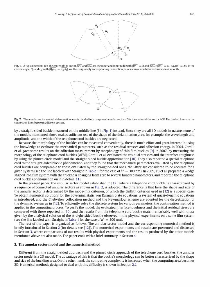
Fig. 1. A typical section: O is the center of the sector, OA1 and OA2 are the outer and inner radii with |OA1| = R and |OA2|/|OA1| = r0 , A1OB1 = 2θ0 is thecentral angle. Q1 and Q2 with |Q1A1| = |Q2B2| are the reciprocally corresponding connection points across which the deformation is smooth.

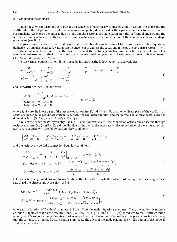
Fig. 2. The annular sector model: delamination area is divided into congruent annular sectors. O is the center of the sector AOB. The dashed lines are theconnection lines between adjacent sectors.

by a straight-sided buckle measured on the middle line (l in Fig. 1) instead. Since they are all 1D models in nature, none ofthe models mentioned above makes sufficient use of the shape of the delamination area, for example, the wavelength andamplitude, and the width of the telephone cord buckles are neglected.

Because the morphology of the buckles can be measured conveniently, there is much effort and great interest in usingthe knowledge to evaluate the mechanical parameters, such as the residual stresses and adhesion energy. In 2004, Cordillet al. gave some results on the adhesion measurement by morphology of thin film buckles [9]. In 2007, by measuring themorphology of the telephone cord buckles (AFM), Cordill et al. evaluated the residual stresses and the interface toughnessby using the pinned circle model and the straight-sided buckle approximation [10]. They also reported a special telephonecord to the straight-sided buckle phenomenon, and they found that the mechanical parameters evaluated by the telephonecord buckles are comparable to those evaluated by the straight-sided ones, the latter are considered to be accurate for agiven system (see the line labeled with Straight in Table 1 for the case of h∗

= 300 nm). In 2009, Yu et al. prepared a wedgeshaped iron film systemwith the thickness changing from zero to several hundred nanometers, and reported the telephonecord buckles phenomenon on it in detail [11].

In the present paper, the annular sector model established in [12], where a telephone cord buckle is characterized bya sequence of connected annular sectors as shown in Fig. 2, is adopted. The difference is that here the shape and size ofthe annular sector is determined by the mode-mix criterion, of which the Griffith criterion used in [12] is a special case.To obtain numerical solutions for the governing static von Karman plate equations, a system of quasi-dynamic equationsis introduced, and the Chebyshev collocation method and the Newmark-β scheme are adopted for the discretization ofthe dynamic system as in [12]. To efficiently solve the discrete system for various parameters, the continuation method isapplied in the computing process. To verify the model, the evaluated interface toughness and the initial residual stress arecompared with those reported in [10], and the results from the telephone cord buckle match remarkably well with thosegiven by the analytical solution of the straight-sided buckle observed in the physical experiments on a same film system(see the line labeled with Straight in Table 1 for the case of h∗

= 300 nm).The rest of the paper is organized as follows. The annular sector model and the corresponding numerical method is

briefly introduced in Section 2 (for details see [12]). The numerical experiments and results are presented and discussedin Section 3, where comparisons of our results with physical experiments and the results produced by the other modelsmentioned above are also made. The paper ends with a brief summary in Section 4.

2. The annular sector model and the numerical method

Different from the straight-sided approach and the pinned circle approach of the telephone cord buckles, the annularsector model is a 2D model. The advantage of this is that the buckle’s morphology can be better characterized by the shapeand size of the buckling area. On the other hand, the computing complexity is increased when the computing area becomes2D. Numerical methods designed to deal with this difficulty is shown in Section 2.2.

862 S. Wang, Z. Li / Journal of Computational and Applied Mathematics 236 (2011) 860–866

2.1. The annular sector model

To describe a typical telephone cord buckle as a sequence of reciprocally connected annular sectors, the shape and thewidth scale of the telephone cord buckle, which can be completely determined by three parameters, need to be determined.For simplicity, we choose the outer radius R of the annular sector as the scale parameter, the half central angle θ0 and thenormalized inner radius r0, i.e. the ratio of the inner radius against the outer radius, of the annular sector as the shapeparameters (see Fig. 1).

The governing equations of the equilibrium state of the buckle can be reduced to the von Karman plate equationsdefined on an annular sectorΩ∗. Naturally, it is convenient to express the equations in the polar coordinate system (r∗, θ∗)with the annular sector’s center O as the polar origin and the sector’s geometric symmetry line as the polar axis. Forsimplicity, we assume that the initial residual stress is equi-biaxial compressive, in Cartesian coordinates this is expressedas −σxx = −σyy = σ ∗

0 > 0, σxy = 0.The von Karman equation is non-dimensioned by introducing the following normalized variables

u =Ru∗

(h∗)2, v =

Rv∗

(h∗)2, w =

w∗

h∗, r =

r∗

R, θ = θ∗, h =

h∗

R,

σ ∗

c =E

1 − ν2

(πh)2

3(1 − r0)2, σ0 =

σ ∗

0

σ ∗c.

(1)

and is rewritten as (see [12] for details)

2w −4π2

(1 − r0)2σ0w = NW (w, u, v),

LU(u, v)+ NU(w) = 0,LV (u, v)+ NV (w) = 0,

(r, θ) ∈ Ω, (2)

where LU , LV are the linear parts of the last two equations in (2), and NW , NU , NV are the nonlinear parts of the von Karmanequations under polar coordinate system, denotes the Laplacian operator, and the normalized annular sector region isdefined asΩ =

(r, θ)|r0 < r < 1,−θ0 < θ < θ0

.

To reflect the experimental symmetry (l in Fig. 1 is the symmetric axis), the connection of the annular sectors throughreciprocal points (Q1,Q2 in Fig. 1), and the film that is clamped to the substrate on the arched edges of the annular sectors,Eqs. (2) are coupled with the following boundary conditions

w(r0, θ) = 0, w ,r(r0, θ) = 0, u(r0, θ) = 0, v(r0, θ) = 0,w(1, θ) = 0, w ,r(1, θ) = 0, u(1, θ) = 0, v(1, θ) = 0, (3)

and the reciprocally periodic connection boundary conditions

1rk∂kw

∂θ k

(r,−θ0)

=1

(1 + r0 − r)k∂kw

∂θ k

(1+r0−r, θ0)

, k = 0, 1, 2, 3,

u(r,−θ0) = −u(1 + r0 − r, θ0),u ,θ (r,−θ0)

r= −

u ,θ (1 + r0 − r, θ0)1 + r0 − r

,

v(r,−θ0) = v(1 + r0 − r, θ0),v ,θ (r,−θ0)

r=v ,θ (1 + r0 − r, θ0)

1 + r0 − r.

(4)

Let E and ν be Young’s modulus and Poisson’s ratio of the elastic thin film. In the polar coordinate system, the energy releaserate G and the phase angle ψ are given as [13]

G(r0, θ0) =3(1 − ν2)h∗(σ ∗

c )2

8π4E

(w ,rr +

ν

r2w ,rθ )

2+ 12u ,2r

,

ψ(r0, θ0) = arctan

(w ,rr +

ν

r2w ,rθ ) cosω +

√12u ,r sinω

−(w ,rr +ν

r2w ,rθ ) sinω +

√12u ,r cosω

,

(5)

where ω is a function of Dundurs’ parameter [13]. Let ΓI be the mode-I interface toughness. Then, the mode-mix fracturecriterion [14] states that on the fracture front G = Γ (ψ) ≡ ΓI

1 + tan2((1 − ρ)ψ)

. It reduces to the Griffith criterion

when ρ = 1. We choose the mode-mix criterion as our fracture criterion, and choose the shape parameters in such a waythat the variance of ΓI on the fracture front is minimized. The effect of the mode parameter ρ on the output of the model isstudied numerically.

S. Wang, Z. Li / Journal of Computational and Applied Mathematics 236 (2011) 860–866 863

2.2. Numerical treatment

We adopt a partial dynamic approach to solve the static von Karman equations (2). Our aim is to find the equilibriumsolution of the following equations

w ,tt +cw ,t + 2w −

4π2

(1 − r0)2σ0w = NW (w, u, v),

LU(u, v)+ NU(w) = 0,LV (u, v)+ NV (w) = 0,

(r, θ) ∈ Ω. (6)

The Newmark-β (γ = 0.5, β = 0.25) scheme [14] is adopted in temporal discretization of the first equation for w,which is in fact the only equation that is time dependent in Eqs. (6). For simplicity, in NW , u and v take the value of theprevious time step, while w takes the unknown value in the current time step. This simplification will definitely reducetremendous amount of computing cost, though it may also lose some temporal accuracy which is not of much concern fora static solution. The discrete scheme of the first equation of Eqs. (6) is implicit and is solved by fixed point iterations.

The Chebyshev collocationmethod is adopted in spatial discretization. First,wemap thenormalized annular sector regionto a standard computing region Ω =

(x, y)|−1 < x < 1,−1 < y < 1

with x = (2r −1− r0)/(1− r0), y = θ/θ0. The first

equation in Eqs. (6) is of the fourth order for the normalized out-of-plane displacementw, thus the boundary conditions ofw need to be treatedwith special care.With a new variable q, setw(x, y) = (1−x2)q(x, y) [14], then, the clamped boundaryconditions (3) forw reduce to the homogeneous boundary conditions for q, just the same as for u and v, which can be easilyimposed with Gauss–Lobatto collocation points. Let Ti(x) be the Chebyshev polynomials of degree i. The discrete form of thedisplacements u, v andw are given as

wn(x, y) =

M−i=0

N+2−j=0

(1 − x2)qnijTi(x)Tj(y),

un(x, y) =

M−i=0

N−j=0

unijTi(x)Tj(y),

vn(x, y) =

M−i=0

N−j=0

vnijTi(x)Tj(y).

(7)

For the reciprocally periodic connections (4), we have twice as many boundary conditions forw as for u and v. Followingthe idea of constructing the Gauss–Lobatto type collocation points [15], we denote Pi(x) polynomials of degree iwhich formthe sequence of orthogonal polynomials on [−1, 1] with the weight function W (y) = (1 − y2)

32 . Then, we construct the

collocation points for the discrete form (7): the Gauss–Lobatto collocation points in the x direction are used for wn, un, vn(there are (M−1) interior points and 2 boundary points), the Gauss–Lobatto collocation points in the y direction are used forun, vn (there are (N−1) interior points and 2 boundary points), and zeros of PN−1(y) are chosen to be the interior collocationpoints forwn in the y direction, each of the boundary points are used twice in this case tomatch the number of the boundaryconditions [12].

To conclude, we write the fully discrete system as 4(∆t)2

+2c∆t

W n+1

M,N = F(W n+1M,N ,U

nM,N)+

3(∆t)2

+c

2∆t

W n+1

M,N

+ 2 1(∆t)2

+c∆t

W n

M,N −

1(∆t)2

+c

2∆t

W n−1

M,N , (8)

L(Un+1M,N) = f(W n+1

M,N ), (9)

where t is the time step length,W nM,N ,U

nM,N stand for the vector value ofw, (u, v)T at time nt on the interior collocation

points, F ,L and f stand for NW − 2w + 4π2(1 − r0)−2σ0w, (LU , LV )T ,−(NU ,NV )

T , respectively. As mentioned before,the first equation of (8) is solved by the fixed point iterations 4

(∆t)2+

2c∆t

W n+1,k+1

M,N = F(W n+1,kM,N ,Un

M,N)+

3(∆t)2

+c

2∆t

W n+1,k

M,N

+ 2 1(∆t)2

+c∆t

W n

M,N −

1(∆t)2

+c

2∆t

W n−1

M,N , (10)

where W n+1,0M,N is set to beW n

M,N .In our numerical experiments, we set M = 20 and N = 10, which turned out to be sufficient to obtain reasonably

accurate numerical results with acceptable efficiency [12].

864 S. Wang, Z. Li / Journal of Computational and Applied Mathematics 236 (2011) 860–866

Fig. 3. The relationship betweenwm = δ/h∗ and σ0 established by the annular sector model with κ = 2.

Fig. 4. The relationship between δ and Γ established by the annular sector model with κ = 2 and h∗= 200 nm.

3. Numerical results and discussions

In this section, our numerical results on the relationship between the geometrical and mechanical parameters arepresented and compared with the experimental and numerical results reported in [10].

3.1. The relationship between the geometrical and mechanical parameters

Since the shape parameter r0 is not easily obtained in physical experiments, to apply our model, we would rather in-troduce another shape parameter that is more easily accessible and more stable in the computation. One such parameteris κ = 4Aλ−1, where A and λ are the wave amplitude and the wavelength of the telephone cord buckles [11], which canbe conveniently measured in experiments and can be expressed, in the annular sector model, as functions of the shapeparameters r0 and θ0 as follows

λ = (1 + r0) sin θ0, A = 2 − (1 + r0) cos θ0. (11)

By choosing κ and θ0 as independent shape parameters of an annular sector, r0 is then given as

r0 =κ sin θ0 + cos θ0 − 2κ sin θ0 − cos θ0

. (12)

In this subsection, we present numerical results with κ = 2, which is the value measured in Fig. 2(a) in [10]. For a given setof mechanical parameters, the mode-mix criterion is used to obtain the shape parameters (r0(κ, θ0), θ0), and the shape andsize of the corresponding buckle is then completely determined. The numerical results on such a relationship (see Fig. 3)can now be used conversely to obtain mechanical parameters, such as the initial stress σ0 and the interface toughness ΓIand Γ (ψ) (see Fig. 4), of the elastic thin film system from the shape and size parameters measured in the telephone cordbuckles observed in physical experiments. Other than κ and θ0, another parameter we use for evaluating σ0 is themaximumout-of-plane displacement δ, the measurements of which will be taken either on the whole buckling area or restricted to

S. Wang, Z. Li / Journal of Computational and Applied Mathematics 236 (2011) 860–866 865

Table 1Recovered values of the initial residual stress and interface toughness with κ = 2 by the annular sector model, compared with the data obtained withthree 1D models in [10], wherewm = δ/h∗ .

h∗ (nm) Meas/model δ (µm) wm (ratio) σ ∗

0 (GPa) σ0 (ratio) ΓI (J/m2) Γ (ψ) (J/m2)

A-S/C 0.633 3.17 4.8 9.5 4.8 16.3200 A-S/A 0.67 3.33 5.3 10.5 4.8 16.5(Case 1) Str-str 0.633 3.17 4.7 5.96 9.56

Curv-str 0.67 3.33 4.75 9.43 6.01Pincrc-pincrc 0.67 3.33 3.74 6.87 2.93

A-S/C 1.47 4.9 2.14 18.8 0.4 1.58A-S/A 1.73 5.77 1.87 22.8 0.14 0.61

300 Straight 1.31 4.7 2.07 15.4 1.6(Case 2) Str-str 1.47 4.9 2.18 19.1 1.8

Curv-str 1.73 5.77 2.14 26.1 1.67Pincrc-pincrc 1.73 5.77 1.64 18.5 0.86

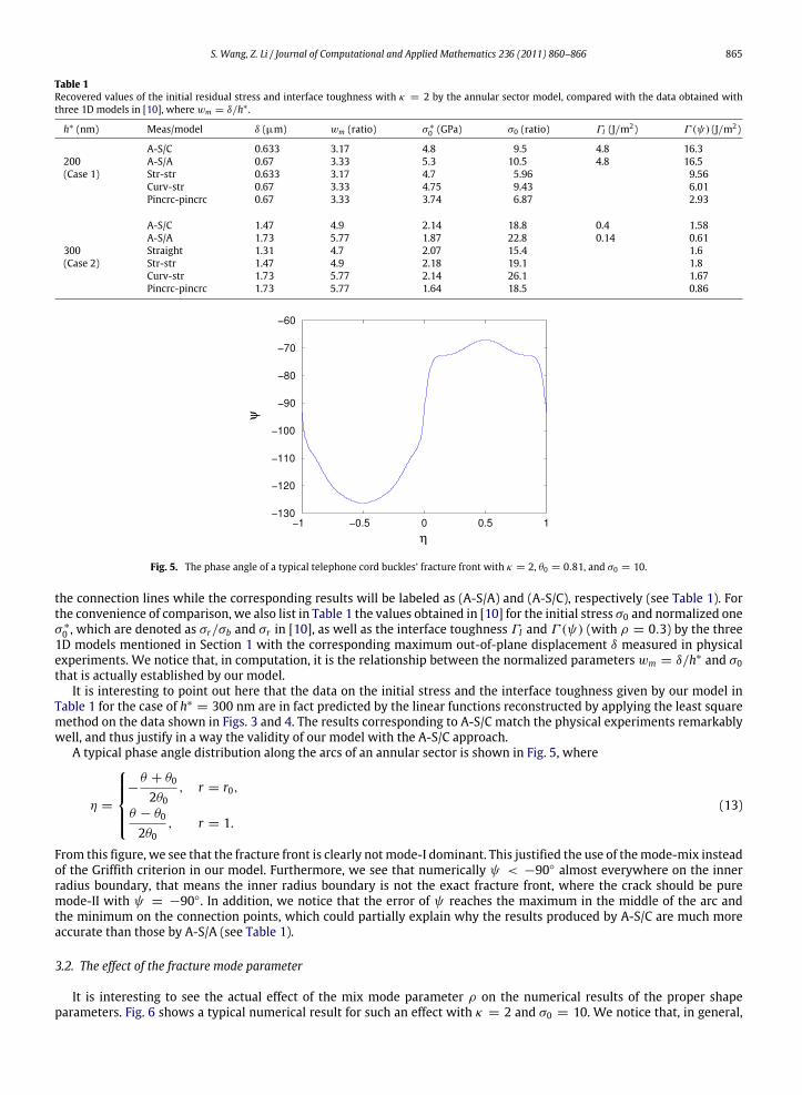
Fig. 5. The phase angle of a typical telephone cord buckles’ fracture front with κ = 2, θ0 = 0.81, and σ0 = 10.

the connection lines while the corresponding results will be labeled as (A-S/A) and (A-S/C), respectively (see Table 1). Forthe convenience of comparison, we also list in Table 1 the values obtained in [10] for the initial stress σ0 and normalized oneσ ∗

0 , which are denoted as σr/σb and σr in [10], as well as the interface toughness ΓI and Γ (ψ) (with ρ = 0.3) by the three1D models mentioned in Section 1 with the corresponding maximum out-of-plane displacement δ measured in physicalexperiments. We notice that, in computation, it is the relationship between the normalized parameters wm = δ/h∗ and σ0that is actually established by our model.

It is interesting to point out here that the data on the initial stress and the interface toughness given by our model inTable 1 for the case of h∗

= 300 nm are in fact predicted by the linear functions reconstructed by applying the least squaremethod on the data shown in Figs. 3 and 4. The results corresponding to A-S/C match the physical experiments remarkablywell, and thus justify in a way the validity of our model with the A-S/C approach.

A typical phase angle distribution along the arcs of an annular sector is shown in Fig. 5, where

η =

−θ + θ0

2θ0, r = r0,

θ − θ0

2θ0, r = 1.

(13)

From this figure, we see that the fracture front is clearly notmode-I dominant. This justified the use of themode-mix insteadof the Griffith criterion in our model. Furthermore, we see that numerically ψ < −90 almost everywhere on the innerradius boundary, that means the inner radius boundary is not the exact fracture front, where the crack should be puremode-II with ψ = −90. In addition, we notice that the error of ψ reaches the maximum in the middle of the arc andthe minimum on the connection points, which could partially explain why the results produced by A-S/C are much moreaccurate than those by A-S/A (see Table 1).

3.2. The effect of the fracture mode parameter

It is interesting to see the actual effect of the mix mode parameter ρ on the numerical results of the proper shapeparameters. Fig. 6 shows a typical numerical result for such an effect with κ = 2 and σ0 = 10. We notice that, in general,

866 S. Wang, Z. Li / Journal of Computational and Applied Mathematics 236 (2011) 860–866

a b

Fig. 6. The relationship between ρ and the shape parameters r0, θ0 with κ = 2, σ0 = 10.

there is essentially no effect for ρ < 0.5, while the effect is clearly not negligible for ρ > 0.5. In fact, the effect of ρ on r0should be considered quite significant for ρ > 0.5. We would also like to point out here that the result shown in Fig. 6 istypical in the sense that for various normalized initial residual stress σ0, the graphs are qualitatively the same, in particular,the value of the proper shape parameter θ0 changes only slightly (within 5% when σ0 varies from 8 to 14).

4. Conclusion

For a given set of mechanical parameters, the morphology of the telephone cord buckles developed on an elastic thinfilm system can be fully determined numerically by the 2D annular sector model coupled with the mode-mix fracturecriterion. This in fact establishes a relationship between the mechanical parameters of the elastic thin film system and thegeometrical parameters of the telephone cord buckles. It turns out that the relationship can be used to evaluate the system’smechanical parameters by the measurements of some easily accessible shape and size parameters of the telephone cordbuckles observed in physical experiments. The numerical results match well with the physical experiments and justify theuse of the mode-mix fracture criterion. Furthermore, for the telephone cord buckles, the mechanical parameters recoveredby our 2D model are in general much more accurate than those evaluated by the three well known 1D models.

Acknowledgments

This research was supported in part by the NSFC project 10871011 and RFDP of China.

References

[1] A.G. Evans, D.R.Mumm, J.W.Hutchinson, G.H.Meier, F.S. Pettic,Mechanisms controlling the durability of thermal barrier coatings, Progress inMaterialsScience 46 (2001) 505–553.

[2] Y. Fu, H. Du, W. Huang, S. Zhang, M. Hu, TiNi-based thin films in MEMS applications: a review, Sensors and Actuators A: Physical 112 (2004) 395–408.[3] P.J. Grundy, Thin film magnetic recording media, Journal of Physics-London-d Applied Physics 31 (1998) 2975.[4] A.S. Argon, V. Gupta, H.S. Landis, J.A. Cornie, Intrinsic toughness of interfaces between SiC coatings and substrates of Si or C fibre, Journal of Materials

Science 24 (1989) 1207–1218.[5] V. Sergo, D.R. Clarke, Observation of subcritical spall propagation of a thermal barrier coating, Journal of the American Ceramic Society 81 (1998)

3237–3242.[6] N. Matuda, S. Bada, A. Kinbara, Internal stress, Young’s modulus and adhesion energy of carbon films on glass substrates, Thin Solid Films 81 (1981)

301–305.[7] G. Gioia, M. Ortiz, Delamination of compressed thin films, Advances in Applied Mechanics 33 (1997) 119–192.[8] M.W.Moon, H.M. Jensen, J.W. Hutchinson, K.H. Oh, A.G. Evans, The characterization of telephone cord buckling of compressed thin films on substrates,

Journal of the Mechanics and Physics of Solids 50 (2002) 2355–2377.[9] M. Cordill, D. Bahr, N. Moody, W. Gerberich, Recent developments in thin film adhesion measurement, IEEE Transactions on Device and Materials

Reliability 4 (2) (2004) 163–168.[10] M. Cordill, D. Bahr, N. Moody, W. Gerberich, Adhesion measurements using telephone cord buckles, Materials Science and Engineering A 443 (2007)

150–155.[11] S. Yu, Y. Zhang, M. Chen, Telephone cord buckles in wedge-shaped Fe films sputtering deposited on glass substrates, Thin Solid Films 518 (2009)

222–226.[12] S. Wang, Z.-P. Li, Mathematical modeling and numerical simulation of telephone cord buckles of elastic films, Science China. Mathematics 54 (5)

(2011) 1063–1076.[13] J.W. Hutchinson, Z. Suo, Mixed mode cracking in layered materials, Advances in Applied Mechanics 29 (1992) 63–191.[14] Z. Yosibash, R.M. Kirby, D. Gottlieb, Collocation methods for the solution of von Karman dynamic non-linear plate systems, Journal of Computational

Physics 200 (2004) 432–461.[15] J. Shen, T. Tang, Spectral and High-order Methods with Applications, Science Press, Beijing, 2006.