Evaluation of Inversion of Final Tile Product to Backscatter, AMM1

Introduction: The Antarctic Mapping Mission (AMM1) products were distributed in a form that minimized radiometric artifacts in the Final Tile Product. Distributed as such, the products required invertible smoothing functions to be applied to the input data, and software for inverting the data from the “smoothed” version to backscatter values (“sigma naught” or σº). Such a system allowed for the distribution of a single product. The software distributed with the final AMM1 product for inverting the data is “GETSIG0,” an ASCII C program which inverts all the radiometric functions applied to Final Tile Product on a coordinate-by-coordinate basis.

The second Antarctic Mapping Mission (MAMM) has a distribution scheme similar to AMM1, including a Final Tile Product which minimizes radiometric artifacts. Upon the completion of the ascending mosaic of MAMM, and with the additional storage capacities now inexpensive with modern hardware, it has become possible to address scientific questions regarding the differences in σº between mosaics. Thus, inversion of the entire AMM1 and MAMM mosaics to σº values has become desirable.

Unfortunately, performance limitations to the GETSIG0 code prevent large scale comparisons of AMM1 and MAMM from easily being completed. James Miller at Vexcel, the vendor which originally completed the GETSIG0 code, improved the speed with which the code executes by completing calculations on an entire tile, rather than on individual coordinates, thus making inverted AMM1 and MAMM mosaics possible.

The aim of this project is to evaluate the quality of the σº values that are the output from Tilesig as applied to the AMM1 product by comparing them to values from GETSIG0, as well as σº values derived directly from slant range SAR and orthorectified SAR imagery, both imagery types which require no radiometric inversion.

Procedure: Evaluation of σº from the final tile product requires derivation of σº from two orthorectified sources: the final tile product, and the orthorectified SAR imagery. It also requires data from a non-geocoded source, the original ingested slant range SAR. Slant range SAR is not in geographic (map) coordinates, but rather in slant range coordinates. It is thus compressed in the across track direction, and has a range of effective ground resolutions. As such, it is difficult or impossible, when paired with geocoded data, to compare individual geographic points. The problem of comparing individual geographic points is overcome when the approximate same areas are selected in the slant range and orthorectified imagery, and global statistics such as histograms, mean, median, mode, and standard deviation are compared. As such, global characteristics were used in the evaluation of the inverted final tile product

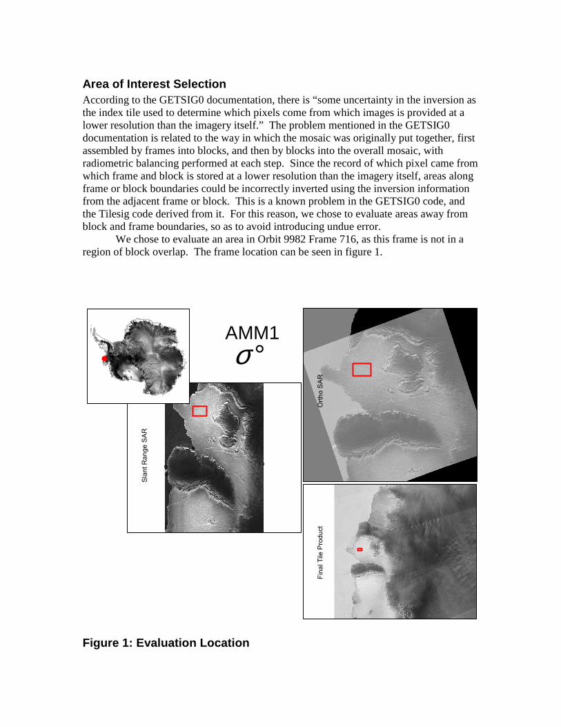
Area of Interest Selection According to the GETSIG0 documentation, there is “some uncertainty in the inversion as the index tile used to determine which pixels come from which images is provided at a lower resolution than the imagery itself.” The problem mentioned in the GETSIG0 documentation is related to the way in which the mosaic was originally put together, first assembled by frames into blocks, and then by blocks into the overall mosaic, with radiometric balancing performed at each step. Since the record of which pixel came from which frame and block is stored at a lower resolution than the imagery itself, areas along frame or block boundaries could be incorrectly inverted using the inversion information from the adjacent frame or block. This is a known problem in the GETSIG0 code, and the Tilesig code derived from it. For this reason, we chose to evaluate areas away from block and frame boundaries, so as to avoid introducing undue error. We chose to evaluate an area in Orbit 9982 Frame 716, as this frame is not in a region of block overlap. The frame location can be seen in figure 1.

AMM1 Sigma0 Evaluation

Sla

nt

Ra

ng

e S

AR

Ort

ho

SA

RF

ina

l T

ile P

rod

uct

AMM1 °σ

Figure 1: Evaluation Location

Data Extraction Images were subset in ERDAS Imagine to approximately the same homogenous “bright” area in each of the slant range image, the ortho, and the tile overview. The pixel values for these areas were exported into an ASCII file from ERDAS using “Utilities: Convert Pixels to ASCII”. From the resultant ASCII files σº values were calculated from DN values in Microsoft Excel using the following equations: Tilesig Final Tile Product conversion from signed 16-bit:

( )30

35.1638

32766__16 −+

=° − dBscaledbitDNσ

Slant range and orthorectified SAR conversion:

−×=° − 0005.0

6000log20 __16

10amplitudescaledbitDN

σ

where DN is the digital number from the imagery.

The lists of coordinates in the ASCII output were also used in a script to extract σº values directly from the GETSIG0 code.

σº values were inverted to Power for analysis of the number of looks:

°

= 1010σ

Power

Statistics Statistics for the analysis of the ASCII output were generated in Matlab. Histograms were generated from the imported array of values for each file using the hist() command. Mean, median, mode, and standard deviation were calculated on the arrays as well.

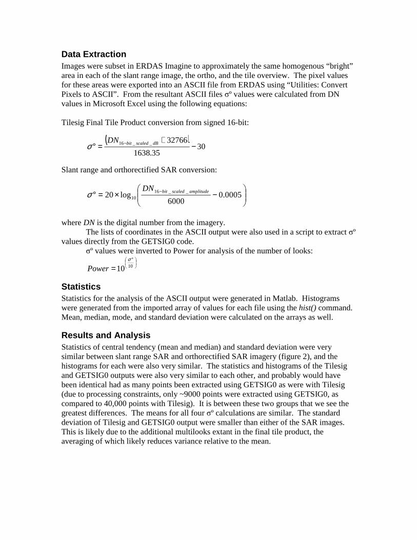
Results and Analysis Statistics of central tendency (mean and median) and standard deviation were very similar between slant range SAR and orthorectified SAR imagery (figure 2), and the histograms for each were also very similar. The statistics and histograms of the Tilesig and GETSIG0 outputs were also very similar to each other, and probably would have been identical had as many points been extracted using GETSIG0 as were with Tilesig (due to processing constraints, only ~9000 points were extracted using GETSIG0, as compared to 40,000 points with Tilesig). It is between these two groups that we see the greatest differences. The means for all four σº calculations are similar. The standard deviation of Tilesig and GETSIG0 output were smaller than either of the SAR images. This is likely due to the additional multilooks extant in the final tile product, the averaging of which likely reduces variance relative to the mean.

Figure 2: Histograms

-12 -10 -8 -6 -4 -2 0 2 4 6 80

100

200

300

400

500

600

700

Fre

quen

cy

-12 -10 -8 -6 -4 -2 0 2 4 6 80

50

100

150

200

250

300

350

400

Fre

quen

cy

-12 -10 -8 -6 -4 -2 0 2 4 6 80

50

100

150

200

250

300

350

Fre

quen

cy

-12 -10 -8 -6 -4 -2 0 2 4 6 80

10

20

30

40

50

60

70

80

90

Sigma 0

Fre

quen

cy

mean: -0.675

median: -0.607

mode: -1.1367

stdev: 1.8196

mean: -0.6938

median: -0.6272

mode: -1.5006

stdev: 1.8197

mean: -0.6209

median: -0.5918

mode: -0.5972

stdev: 1.3973

mean: -0.6152

median: -0.5957

mode: -0.8669

stdev: 1.3988

0 0.5 1 1.5 2 2.5 3 3.5 4 4.50

100

200

300

400

500

600

700

800

900

Fre

quen

cy

0 0.5 1 1.5 2 2.5 3 3.5 4 4.50

50

100

150

200

250

300

350

400

Fre

quen

cy

0 0.5 1 1.5 2 2.5 3 3.5 4 4.50

50

100

150

200

250

300

350

400

450

Fre

quen

cy

0 0.5 1 1.5 2 2.5 3 3.5 4 4.50

10

20

30

40

50

60

70

80

90

Power

Fre

quen

cy

Poweroσ

Fre

quen

cymean: 0.932stdev: 0.3886ratio: 0.416953

mean: 0.928stdev: 0.3862ratio: 0.416164

mean: 0.9122stdev: 0.2949ratio: 0.323284

mean: 0.9136stdev: 0.2969ratio: 0.324978

Sla

nt R

ange

SA

RO

rtho

SA

RF

inal

Tile

: Tile

sig

Fin

al T

ile: G

ET

SIG

0

-12 -10 -8 -6 -4 -2 0 2 4 6 80

100

200

300

400

500

600

700

Fre

quen

cy

-12 -10 -8 -6 -4 -2 0 2 4 6 80

50

100

150

200

250

300

350

400

Fre

quen

cy

-12 -10 -8 -6 -4 -2 0 2 4 6 80

50

100

150

200

250

300

350

Fre

quen

cy

-12 -10 -8 -6 -4 -2 0 2 4 6 80

10

20

30

40

50

60

70

80

90

Sigma 0

Fre

quen

cy

mean: -0.675

median: -0.607

mode: -1.1367

stdev: 1.8196

mean: -0.6938

median: -0.6272

mode: -1.5006

stdev: 1.8197

mean: -0.6209

median: -0.5918

mode: -0.5972

stdev: 1.3973

mean: -0.6152

median: -0.5957

mode: -0.8669

stdev: 1.3988

0 0.5 1 1.5 2 2.5 3 3.5 4 4.50

100

200

300

400

500

600

700

800

900

Fre

quen

cy

0 0.5 1 1.5 2 2.5 3 3.5 4 4.50

50

100

150

200

250

300

350

400

Fre

quen

cy

0 0.5 1 1.5 2 2.5 3 3.5 4 4.50

50

100

150

200

250

300

350

400

450

Fre

quen

cy

0 0.5 1 1.5 2 2.5 3 3.5 4 4.50

10

20

30

40

50

60

70

80

90

Power

Fre

quen

cy

Poweroσ

Fre

quen

cymean: 0.932stdev: 0.3886ratio: 0.416953

mean: 0.928stdev: 0.3862ratio: 0.416164

mean: 0.9122stdev: 0.2949ratio: 0.323284

mean: 0.9136stdev: 0.2969ratio: 0.324978

-12 -10 -8 -6 -4 -2 0 2 4 6 80

100

200

300

400

500

600

700

Fre

quen

cy

-12 -10 -8 -6 -4 -2 0 2 4 6 80

50

100

150

200

250

300

350

400

Fre

quen

cy

-12 -10 -8 -6 -4 -2 0 2 4 6 80

50

100

150

200

250

300

350

Fre

quen

cy

-12 -10 -8 -6 -4 -2 0 2 4 6 80

10

20

30

40

50

60

70

80

90

Sigma 0

Fre

quen

cy

mean: -0.675

median: -0.607

mode: -1.1367

stdev: 1.8196

mean: -0.6938

median: -0.6272

mode: -1.5006

stdev: 1.8197

mean: -0.6209

median: -0.5918

mode: -0.5972

stdev: 1.3973

mean: -0.6152

median: -0.5957

mode: -0.8669

stdev: 1.3988

0 0.5 1 1.5 2 2.5 3 3.5 4 4.50

100

200

300

400

500

600

700

800

900

Fre

quen

cy

0 0.5 1 1.5 2 2.5 3 3.5 4 4.50

50

100

150

200

250

300

350

400

Fre

quen

cy

0 0.5 1 1.5 2 2.5 3 3.5 4 4.50

50

100

150

200

250

300

350

400

450

Fre

quen

cy

0 0.5 1 1.5 2 2.5 3 3.5 4 4.50

10

20

30

40

50

60

70

80

90

Power

Fre

quen

cy

-12 -10 -8 -6 -4 -2 0 2 4 6 80

100

200

300

400

500

600

700

Fre

quen

cy

-12 -10 -8 -6 -4 -2 0 2 4 6 80

50

100

150

200

250

300

350

400

Fre

quen

cy

-12 -10 -8 -6 -4 -2 0 2 4 6 80

50

100

150

200

250

300

350

Fre

quen

cy

-12 -10 -8 -6 -4 -2 0 2 4 6 80

10

20

30

40

50

60

70

80

90

Sigma 0

Fre

quen

cy

mean: -0.675

median: -0.607

mode: -1.1367

stdev: 1.8196

mean: -0.6938

median: -0.6272

mode: -1.5006

stdev: 1.8197

mean: -0.6209

median: -0.5918

mode: -0.5972

stdev: 1.3973

mean: -0.6152

median: -0.5957

mode: -0.8669

stdev: 1.3988

0 0.5 1 1.5 2 2.5 3 3.5 4 4.50

100

200

300

400

500

600

700

800

900

Fre

quen

cy

0 0.5 1 1.5 2 2.5 3 3.5 4 4.50

50

100

150

200

250

300

350

400

Fre

quen

cy

0 0.5 1 1.5 2 2.5 3 3.5 4 4.50

50

100

150

200

250

300

350

400

450

Fre

quen

cy

0 0.5 1 1.5 2 2.5 3 3.5 4 4.50

10

20

30

40

50

60

70

80

90

Power

Fre

quen

cy

-12 -10 -8 -6 -4 -2 0 2 4 6 80

100

200

300

400

500

600

700

Fre

quen

cy

-12 -10 -8 -6 -4 -2 0 2 4 6 80

50

100

150

200

250

300

350

400

Fre

quen

cy

-12 -10 -8 -6 -4 -2 0 2 4 6 80

50

100

150

200

250

300

350

Fre

quen

cy

-12 -10 -8 -6 -4 -2 0 2 4 6 80

10

20

30

40

50

60

70

80

90

Sigma 0

Fre

quen

cy

mean: -0.675

median: -0.607

mode: -1.1367

stdev: 1.8196

mean: -0.6938

median: -0.6272

mode: -1.5006

stdev: 1.8197

mean: -0.6209

median: -0.5918

mode: -0.5972

stdev: 1.3973

mean: -0.6152

median: -0.5957

mode: -0.8669

stdev: 1.3988

-12 -10 -8 -6 -4 -2 0 2 4 6 80

100

200

300

400

500

600

700

Fre

quen

cy

-12 -10 -8 -6 -4 -2 0 2 4 6 80

50

100

150

200

250

300

350

400

Fre

quen

cy

-12 -10 -8 -6 -4 -2 0 2 4 6 80

50

100

150

200

250

300

350

Fre

quen

cy

-12 -10 -8 -6 -4 -2 0 2 4 6 80

10

20

30

40

50

60

70

80

90

Sigma 0

Fre

quen

cy

-12 -10 -8 -6 -4 -2 0 2 4 6 80

100

200

300

400

500

600

700

Fre

quen

cy

-12 -10 -8 -6 -4 -2 0 2 4 6 80

50

100

150

200

250

300

350

400

Fre

quen

cy

-12 -10 -8 -6 -4 -2 0 2 4 6 80

50

100

150

200

250

300

350

Fre

quen

cy

-12 -10 -8 -6 -4 -2 0 2 4 6 80

10

20

30

40

50

60

70

80

90

Sigma 0

Fre

quen

cy

mean: -0.675

median: -0.607

mode: -1.1367

stdev: 1.8196

mean: -0.6938

median: -0.6272

mode: -1.5006

stdev: 1.8197

mean: -0.6209

median: -0.5918

mode: -0.5972

stdev: 1.3973

mean: -0.6152

median: -0.5957

mode: -0.8669

stdev: 1.3988

0 0.5 1 1.5 2 2.5 3 3.5 4 4.50

100

200

300

400

500

600

700

800

900

Fre

quen

cy

0 0.5 1 1.5 2 2.5 3 3.5 4 4.50

50

100

150

200

250

300

350

400

Fre

quen

cy

0 0.5 1 1.5 2 2.5 3 3.5 4 4.50

50

100

150

200

250

300

350

400

450

Fre

quen

cy

0 0.5 1 1.5 2 2.5 3 3.5 4 4.50

10

20

30

40

50

60

70

80

90

Power

Fre

quen

cy

0 0.5 1 1.5 2 2.5 3 3.5 4 4.50

100

200

300

400

500

600

700

800

900

Fre

quen

cy

0 0.5 1 1.5 2 2.5 3 3.5 4 4.50

50

100

150

200

250

300

350

400

Fre

quen

cy

0 0.5 1 1.5 2 2.5 3 3.5 4 4.50

50

100

150

200

250

300

350

400

450

Fre

quen

cy

0 0.5 1 1.5 2 2.5 3 3.5 4 4.50

10

20

30

40

50

60

70

80

90

Power

Fre

quen

cy

0 0.5 1 1.5 2 2.5 3 3.5 4 4.50

100

200

300

400

500

600

700

800

900

Fre

quen

cy

0 0.5 1 1.5 2 2.5 3 3.5 4 4.50

50

100

150

200

250

300

350

400

Fre

quen

cy

0 0.5 1 1.5 2 2.5 3 3.5 4 4.50

50

100

150

200

250

300

350

400

450

Fre

quen

cy

0 0.5 1 1.5 2 2.5 3 3.5 4 4.50

10

20

30

40

50

60

70

80

90

Power

Fre

quen

cy

Poweroσ

Fre

quen

cymean: 0.932stdev: 0.3886ratio: 0.416953

mean: 0.928stdev: 0.3862ratio: 0.416164

mean: 0.9122stdev: 0.2949ratio: 0.323284

mean: 0.9136stdev: 0.2969ratio: 0.324978

Sla

nt R

ange

SA

RO

rtho

SA

RF

inal

Tile

: Tile

sig

Fin

al T

ile: G

ET

SIG

0

Data Format for All Sigma 0 Products As mentioned in the Data Extraction Section, sigma naught dB data output are scaled to 16-bit binary for storage and transfer purposes from the Tilesig Code. For consistency and storage purposes, the same equation is used for all sig0 products.

( )( ) 327663035.1638__16 −+°×=− dBdBscaledbitDN σ

Null values are stored as -32767. Ignoring null values, conversion from 16-bit scaled dB to dB requires the following inverse equation.

( )30

35.1638

32766__16 −+

=° − dBscaledbitDNσ

Projection information All sig0 products are distributed in South Pole Polar Stereographic. Latitude of true scale is -71°, thus making the scaling factor 0.97276901289.

Processing Information Data for the AMM1 Sig0 Mosaic were processed first using the tilesig code developed by Vexcel in order to invert the radiometric corrections applied to the dataset. The data were then converted to a linear form of sigma naught for resampling to coarser resolution tiers, 50m, 100m, 200m, 400m, and 800m tiers. The tiers were then mosaic’d, converted back to a scaled 16-bit version of sigma naught, and also an unscaled 32-bit version.

100,200400,800mlinear sig0

tiers mosaic

100,200400,800mmosaics

(dB)

100,200400,800m

Tiers(scaled dB)

AMM1Tiles

tilesig25m scaled

dBtiers

dB tolinear

25m linearsig0tiers

degrade

(50),100,200400,800mlinear sig0

tiers

linear toscaled dB

mosaic

Scaled dBto dBfloat

Figure 3: AMM1 sig0 Block Diagram