PROCEEDINGS, 43rd Workshop on Geothermal Reservoir Engineering

Stanford University, Stanford, California, February 12-14, 2018

SGP-TR-213

1

Multiscale Elastic-Waveform Inversion of 2016 Walkway VSP Data from the Raft River

Geothermal Field

Benxin Chi and Lianjie Huang

Los Alamos National Laboratory, Geophysics Group, Los Alamos, NM 87545, USA

benxinchi@lanl.gov; ljh@lanl.gov

Keywords: Elastic-waveform inversion, Raft River geothermal field, velocity model, vertical seismic profiling.

ABSTRACT

The Raft River geothermal field was selected by the U.S. Department of Energy (DOE) as an Enhanced Geothermal System (EGS)

demonstration project in 2010. Vertical seismic profiling (VSP) data were acquired along five walkaway lines at the Raft River geothermal

field in 2016 for subsurface imaging, particularly for characterizing the Narrows zone for EGS stimulations. The VSP data were recorded

using 84 three-component receivers in well RRG-9. We conduct multiscale elastic-waveform inversion of the VSP data to obtain high-

resolution P- and S-wave velocity models for reservoir characterization and migration imaging. We first build a 1D velocity model from

sonic log data and zero-offset VSP data, and obtain a 3D traveltime tomography velocity model using the first arrivals of down-going

waves in the VSP data. We then conduct multiscale elastic-waveform inversion of rotated and denoised three-component VSP data using

the 3D traveltime tomography velocity models as the initial models. Our preliminary inversion result shows a low-velocity zone that may

be associated with the Narrows zone.

1. INTRODUCTION

The Raft River geothermal field, located in southern Idaho approximately 100 miles northwest of Salt Lake City, Utah (Figure 1), was

selected by the U.S. Department of Energy (DOE) as an Enhanced Geothermal System (EGS) demonstration project in 2010. There are

four production wells in Raft River geothermal fields: RRG 1, 2 and 4 located on the northwest side of the field (Figure 1) and RRG-7

situated on the southeast side. It was inferred from geophysical data (Mabey et al., 1978), where production is generally from the

Precambrian basement from depths of 1400 to 1750 m (Ayling et al., 2011; Jones et al., 2011). Geochemical analysis by Ayling et al.

(2011) found different geothermal fluid geochemistries in the southeast and northwest parts of the field. Reservoir fluids from the

northwest (RRG-1,2,4,5) contain lower salinities than those from the southeast (RRG-3,6,7,9,11). Based on these data, Ayling and Moore

(2013) concluded that the northwestern and southeastern portions of the geothermal field are separated by a low permeability shear zone

within the Precambrian basement, which they referred as the Narrows zone (Figure 2). Accurate imaging and characterization of the

Narrows zone is necessary for EGS development at the Raft River geothermal field.

Figure 1: Map of the Raft River geothermal field. Production wells and production pipelines are shown in red. Injection wells and

injection pipelines are shown in blue. Well RRG-9 was used for VSP data acquisition. (Modified from Williams et al., 1982)

Chi and Huang

2

The presence of the Narrows zone is supported by microseismic data collected since August, 2010 (Figure 2) by Lawrence Berkeley

National Laboratory (LBNL). Multiple walkaway vertical seismic profiling (VSP) surveys were conducted in 2016 for building a high-

resolution velocity model, which is needed for accurate microseismic imaging and focal mechanism inversion, and high-resolution

imaging of the underlying structures using VSP data. We apply our recently developed multiscale elastic-waveform inversion method to

the VSP data acquired in 2016 to invert for both P- and S-wave velocity models.

We first briefly describe our multiscale elastic-waveform inversion method, present example VSP data for inversion, build a 1D velocity

model from sonic log data, and give traveltime tomography and multiscale elastic-waveform inversion results obtained using VSP data of

one walkaway line acquired at the Raft River geothermal field in 2016.

Figure 2: Distribution of microseismic events since August, 2010 along the Narrows zone at the Raft River geothermal field (Li et

al., 2017).

2. METHOD

We use a multiscale elastic-waveform inversion method to build velocity models using VSP data. The method combines envelope

inversion and multiscale inversion in both the space and time domains.

Elastic-waveform envelope inversion can produce a low-resolution initial velocity model for elastic-waveform inversion to improve the

convergence. Analog to elastic-waveform inversion, envelope inversion fits data envelope obse with synthetic data envelope

cale by

minimizing the misfit function given by

obs cal

2 2

obs cal

(t) (t)dt1

(t)dt (t)dtE

e em

e e, (1)

where m is elastic parameters to be inverted, and t is time.

Elastic-waveform inversion progressively fits synthetic elastic waveforms cald with recorded elastic waveforms

obsd to obtain elastic

parameters m . The inversion minimizes the following zero-lag cross-correlation objective function:

obs cal

2 2

obs cal

(t) (t)dt1

(t)dt (t)dtE

d dm

d d. (2)

The correlation-based misfit function can suppress some inversion artifacts caused by the difficulty in matching amplitudes of seismic

waveforms in practical applications. Synthetic elastic-waveforms cald are related to model parameters m as

cal fd m , (3)

Chi and Huang

3

where f is the wavefield forward modeling operator. We use an optimized high-order staggered-grid finite-difference algorithm with

convolutional perfectly matched layers for forward and backward propagation of wavefields in elastic-waveform inversion.

In data-domain, low-frequency bandpass filtered data are used at earlier stages of inversion, producing a long-wavelength/low-resolution

model. The inverted model is then used as the initial model at later stages of inversion of higher-frequency bandpass filtered data to

produce a shorter-wavelength/higher-resolution models. With gradually increased the frequency bands, all frequency contents of the

observed data are eventually used for inversion. The objective function of this data-domain multiscale approach can be defined as:

obs cal

2 2

obs cal

(t) (t)dt1

(t) dt (t) dtm

W WE

W W

d dm

d d

, (4)

with the frequency-dependent weights defined as

min max

min max

if1,

if or0,W

, (5)

where min and

max are the minimum and maximum frequency of a frequency band, respectively. In the time domain elastic-waveform

inversion, this scheme is implemented by filtering observed and synthetic data before the gradient computation using the adjoint-state

method.

In our recently developed multiscale elastic-waveform inversion in both the space and time domains, we apply the wavelet transform to

inversion results of different frequency bands of data. Different frequency bands of data should invert for different spatial resolution of

models. The inversion model can be transformed into different spatial scales using the wavelet transform:

X W m , (6)

where X denotes the wavelet transform result of the inversion model, and W is the wavelet basis. Reconstruction of the model reconstrm

is obtained using the inverse wavelet transform:

reconstr

T TW X W W m m . (7)

With Equations (6) and (7), we can obtain multiscale model representations for inversion results of different frequency bands of data. In

our joint data-domain and model-domain multiscale inversion, we employ coarser scales coefficients at earlier stages of elastic-waveform

inversion for lower-frequency data, and gradually add finer scales at later stages of elastic-waveform inversion for higher-frequency data.

3. RESULTS

3.1 Walkaway VSP Data and Initial Model

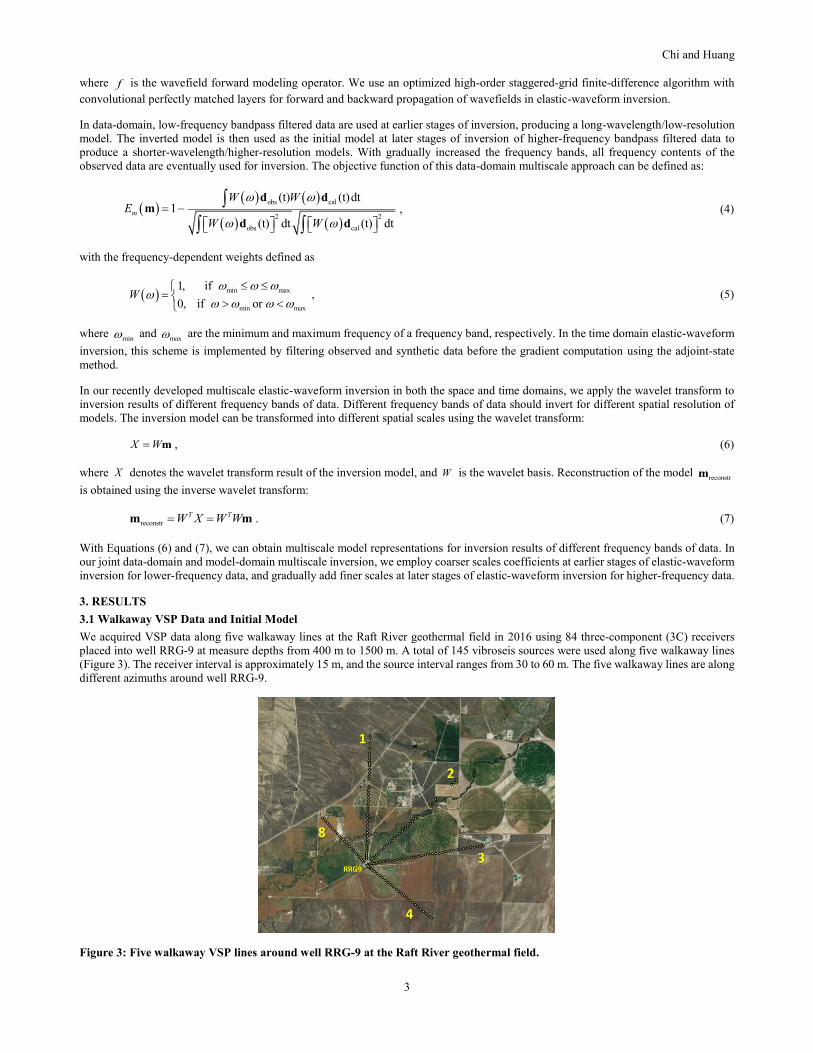
We acquired VSP data along five walkaway lines at the Raft River geothermal field in 2016 using 84 three-component (3C) receivers

placed into well RRG-9 at measure depths from 400 m to 1500 m. A total of 145 vibroseis sources were used along five walkaway lines

(Figure 3). The receiver interval is approximately 15 m, and the source interval ranges from 30 to 60 m. The five walkaway lines are along

different azimuths around well RRG-9.

Figure 3: Five walkaway VSP lines around well RRG-9 at the Raft River geothermal field.

Chi and Huang

4

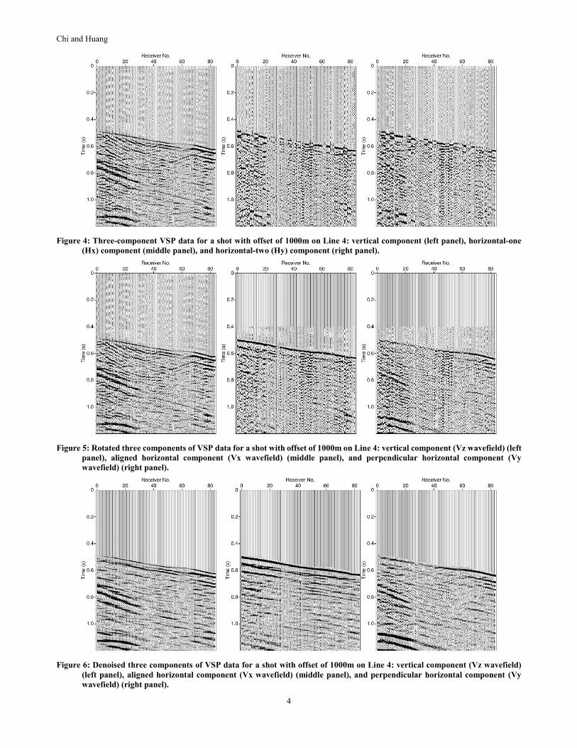
Figure 4: Three-component VSP data for a shot with offset of 1000m on Line 4: vertical component (left panel), horizontal-one

(Hx) component (middle panel), and horizontal-two (Hy) component (right panel).

Figure 5: Rotated three components of VSP data for a shot with offset of 1000m on Line 4: vertical component (Vz wavefield) (left

panel), aligned horizontal component (Vx wavefield) (middle panel), and perpendicular horizontal component (Vy

wavefield) (right panel).

Figure 6: Denoised three components of VSP data for a shot with offset of 1000m on Line 4: vertical component (Vz wavefield)

(left panel), aligned horizontal component (Vx wavefield) (middle panel), and perpendicular horizontal component (Vy

wavefield) (right panel).

Chi and Huang

5

We first rotate and denoise the raw VSP data for our multiscale elastic-waveform inversion. Figure 4-Figure 6 show the raw, rotated and

denoised three-component VSP data for a shot with offset of 1000m on Line 4.

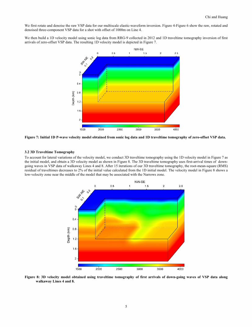
We then build a 1D velocity model using sonic log data from RRG-9 collected in 2012 and 1D traveltime tomography inversion of first

arrivals of zero-offset VSP data. The resulting 1D velocity model is depicted in Figure 7.

Figure 7: Initial 1D P-wave velocity model obtained from sonic log data and 1D traveltime tomography of zero-offset VSP data.

3.2 3D Traveltime Tomography

To account for lateral variations of the velocity model, we conduct 3D traveltime tomography using the 1D velocity model in Figure 7 as

the initial model, and obtain a 3D velocity model as shown in Figure 8. The 3D traveltime tomography uses first-arrival times of down-

going waves in VSP data of walkaway Lines 4 and 8. After 15 iterations of our 3D traveltime tomography, the root-mean-square (RMS)

residual of traveltimes decreases to 2% of the initial value calculated from the 1D initial model. The velocity model in Figure 8 shows a

low-velocity zone near the middle of the model that may be associated with the Narrows zone.

Figure 8: 3D velocity model obtained using traveltime tomography of first arrivals of down-going waves of VSP data along

walkaway Lines 4 and 8.

Chi and Huang

6

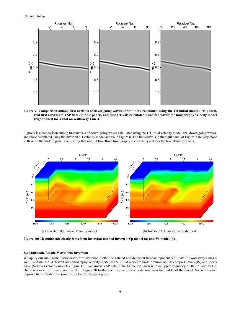
Figure 9: Comparison among first arrivals of down-going waves of VSP data calculated using the 1D initial model (left panel),

real first arrivals of VSP data (middle panel), and first arrivals calculated using 3D traveltime tomography velocity model

(right panel) for a shot on walkaway Line 4.

Figure 9 is a comparison among first arrivals of down-going waves calculated using the 1D initial velocity model, real down-going waves,

and those calculated using the inverted 3D velocity model shown in Figure 8. The first arrivals in the right panel of Figure 9 are very close

to those in the middle panel, confirming that our 3D traveltime tomography successfully reduces the traveltime residuals.

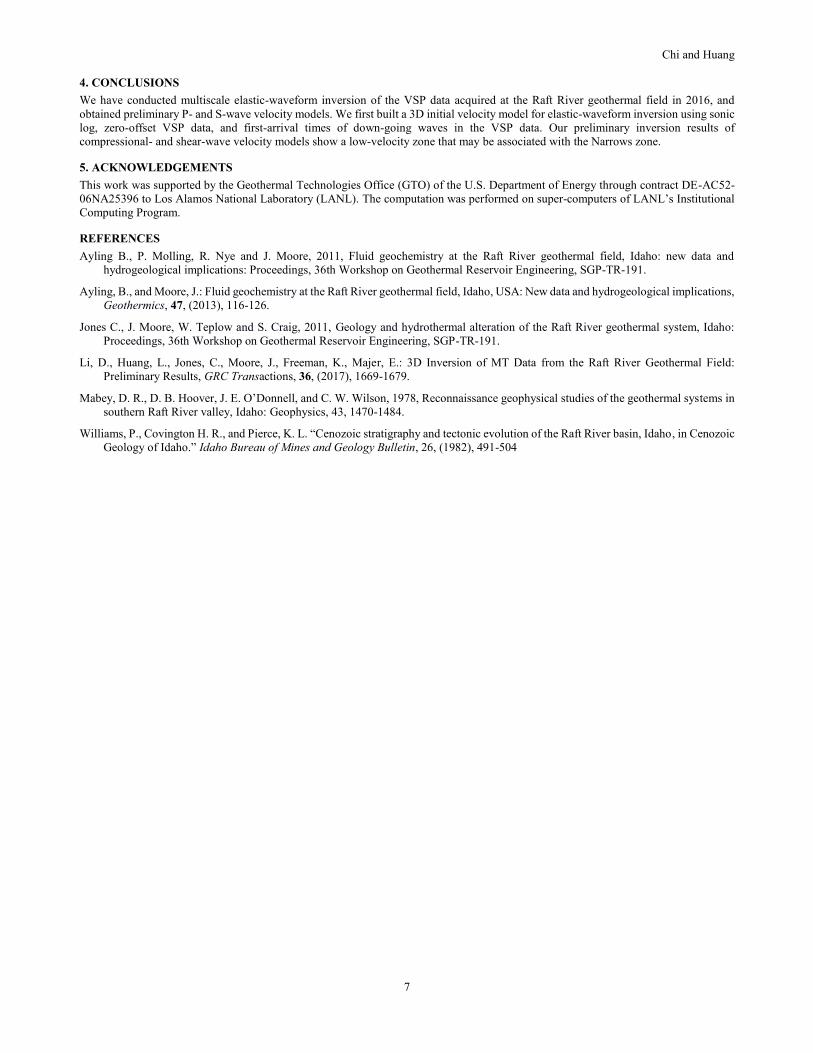
(a) Inverted 3D P-wave velocity model (b) Inverted 3D S-wave velocity model

Figure 10: 3D multiscale elastic-waveform inversion method inverted Vp model (a) and Vs model (b).

3.3 Multiscale Elastic-Waveform Inversion

We apply our multiscale elastic-waveform inversion method to rotated and denoised three-component VSP data for walkaway Lines 4

and 8, and use the 3D traveltime tomography velocity model as the initial model to build preliminary 3D compressional- (P-) and shear-

wave (S-wave) velocity models (Figure 10). We invert VSP data in the frequency bands with an upper frequency of 10, 15, and 25 Hz.

Our elastic-waveform inversion results in Figure 10 further confirm the low-velocity zone near the middle of the model. We will further

improve the velocity inversion results for the deeper regions.

Chi and Huang

7

4. CONCLUSIONS

We have conducted multiscale elastic-waveform inversion of the VSP data acquired at the Raft River geothermal field in 2016, and

obtained preliminary P- and S-wave velocity models. We first built a 3D initial velocity model for elastic-waveform inversion using sonic

log, zero-offset VSP data, and first-arrival times of down-going waves in the VSP data. Our preliminary inversion results of

compressional- and shear-wave velocity models show a low-velocity zone that may be associated with the Narrows zone.

5. ACKNOWLEDGEMENTS

This work was supported by the Geothermal Technologies Office (GTO) of the U.S. Department of Energy through contract DE-AC52-

06NA25396 to Los Alamos National Laboratory (LANL). The computation was performed on super-computers of LANL’s Institutional

Computing Program.

REFERENCES

Ayling B., P. Molling, R. Nye and J. Moore, 2011, Fluid geochemistry at the Raft River geothermal field, Idaho: new data and

hydrogeological implications: Proceedings, 36th Workshop on Geothermal Reservoir Engineering, SGP-TR-191.

Ayling, B., and Moore, J.: Fluid geochemistry at the Raft River geothermal field, Idaho, USA: New data and hydrogeological implications,

Geothermics, 47, (2013), 116-126.

Jones C., J. Moore, W. Teplow and S. Craig, 2011, Geology and hydrothermal alteration of the Raft River geothermal system, Idaho:

Proceedings, 36th Workshop on Geothermal Reservoir Engineering, SGP-TR-191.

Li, D., Huang, L., Jones, C., Moore, J., Freeman, K., Majer, E.: 3D Inversion of MT Data from the Raft River Geothermal Field:

Preliminary Results, GRC Transactions, 36, (2017), 1669-1679.

Mabey, D. R., D. B. Hoover, J. E. O’Donnell, and C. W. Wilson, 1978, Reconnaissance geophysical studies of the geothermal systems in

southern Raft River valley, Idaho: Geophysics, 43, 1470-1484.

Williams, P., Covington H. R., and Pierce, K. L. “Cenozoic stratigraphy and tectonic evolution of the Raft River basin, Idaho, in Cenozoic

Geology of Idaho.” Idaho Bureau of Mines and Geology Bulletin, 26, (1982), 491-504