Evaluation of Fault-Normal/Fault-Parallel Directions Rotated Ground Motions for Response History Analysis of an Instrumented Six-Story Building

By Erol Kalkan and Neal S. Kwong

Prepared in cooperation with the University of California Berkeley

Open-File Report 2012—1058

U.S. Department of the Interior U.S. Geological Survey

U.S. Department of the Interior KEN SALAZAR, Secretary

U.S. Geological Survey Marcia K. McNutt, Director

U.S. Geological Survey, Reston, Virginia: 2012

For product and ordering information:

World Wide Web: http://www.usgs.gov/pubprod/

Telephone: 1-888-ASK-USGS

For more information on the USGS—the Federal source for science about the Earth,

its natural and living resources, natural hazards, and the environment:

World Wide Web: http://www.usgs.gov/

Telephone: 1-888-ASK-USGS

Suggested citation:

Kalkan, E., and Kwong, N.S., 2012, Evaluation of fault-normal/fault-parallel directions rotated ground

motions for response history analysis of an instrumented six-story building: U.S. Geological Survey

Open-File Report 2012-1058, 30 p., available at http://pubs.usgs.gov/of/2012/1058/.

Any use of trade, product, or firm name/ is for descriptive purposes only and does not imply

endorsement by the U.S. Government./

Although this report is in the public domain, permission must be secured from the individual copyright

owners to reproduce any copyrighted material contained within this report.

iii

Contents Abstract ...........................................................................................................................................1 Introduction ......................................................................................................................................1 Description of Structural System and Computer Model ...................................................................3 Ground-Motions Selected ................................................................................................................4 Methodology for Evaluation of Fault-Normal/Fault-Parallel Directions .............................................4 Structural Response Variability with Rotation Angle ........................................................................5 Evaluation of Fault-Normal/Fault-Parallel Directions Rotated Ground Motions................................6 Conclusions .....................................................................................................................................8 Acknowledgments ...........................................................................................................................9 References Cited .............................................................................................................................9

Tables 1. Linear-elastic dynamic properties of the Imperial County Services Building; the modal

participation () and modal contribution factors (MCF) are shown to illustrate how the first six modes contribute to the linear-elastic responses in two orthogonal directions. .................. 12

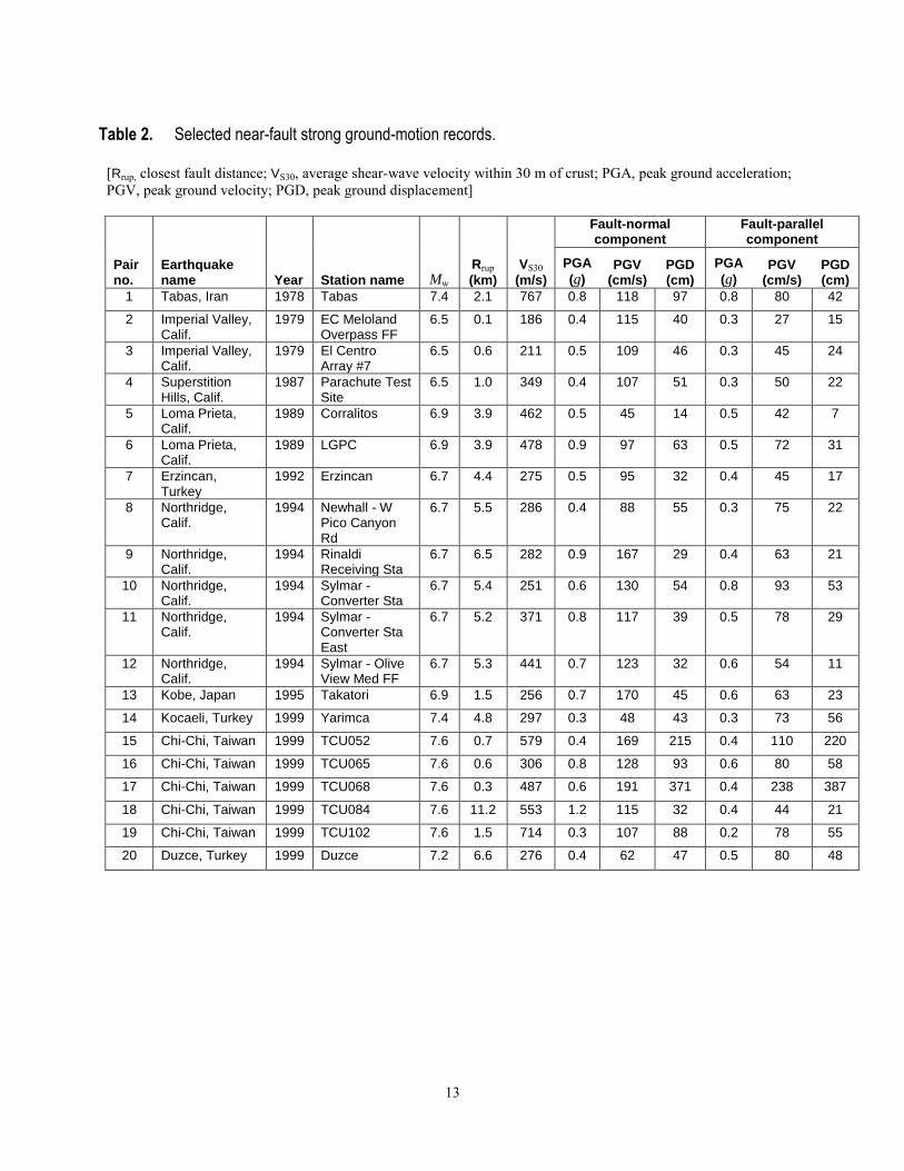
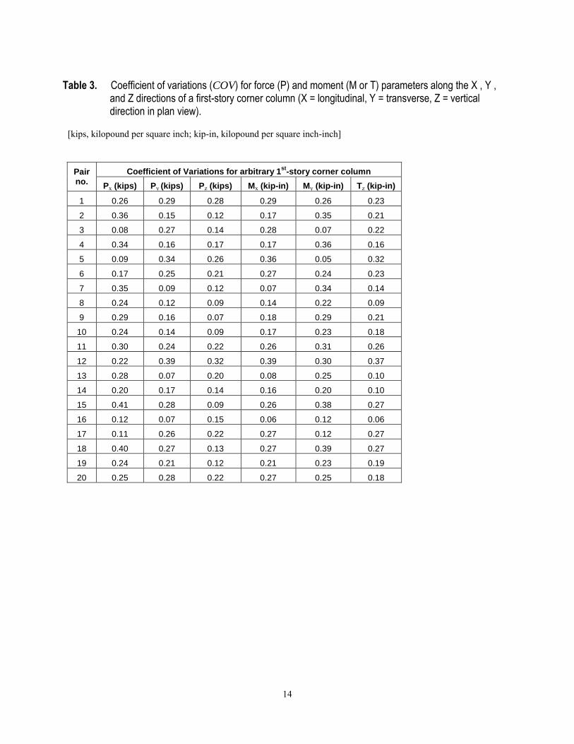
2. Selected near-fault strong ground-motion records. .................................................................. 13 3. Coefficient of variations (COV) for force (P) and moment (M or T) parameters along the X ,

Y , and Z directions of a first-story corner column (X = longitudinal, Y = transverse, Z = vertical direction in plan view). ................................................................................................. 14

4. Probabilities of exceeding the larger response among the fault-normal/fault-parallel (FN/FP) values for selected response quantities, estimated with 5,000 random samples. ....... 15

Figures 1. Imperial County Services Building—(top) general view towards north, (bottom) damage of

ground floor columns during the Mw 6.5 1979 Imperial Valley earthquake. ............................. 16 2. Foundation and ground level plan (top) and typical floor layout (bottom) of the Imperial

County Services Building ......................................................................................................... 17 3. Instrumentation layout of the Imperial County Services Building. ............................................. 18 4. Pseudo-acceleration response spectra of 20 near-fault strong ground motions; damping

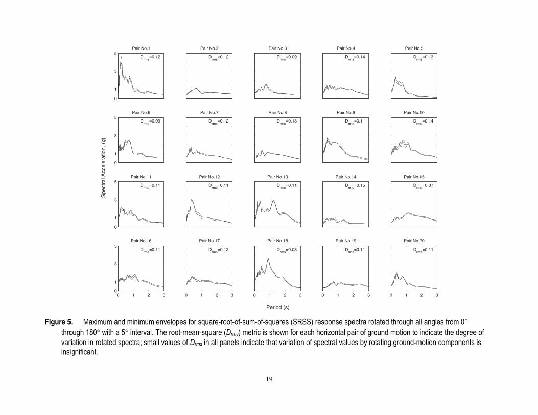
ratio 5 percent .Red, median spectrum of all records; Tn = spectral period. ............................. 18 5. Maximum and minimum envelopes for square-root-of-sum-of-squares (SRSS) response

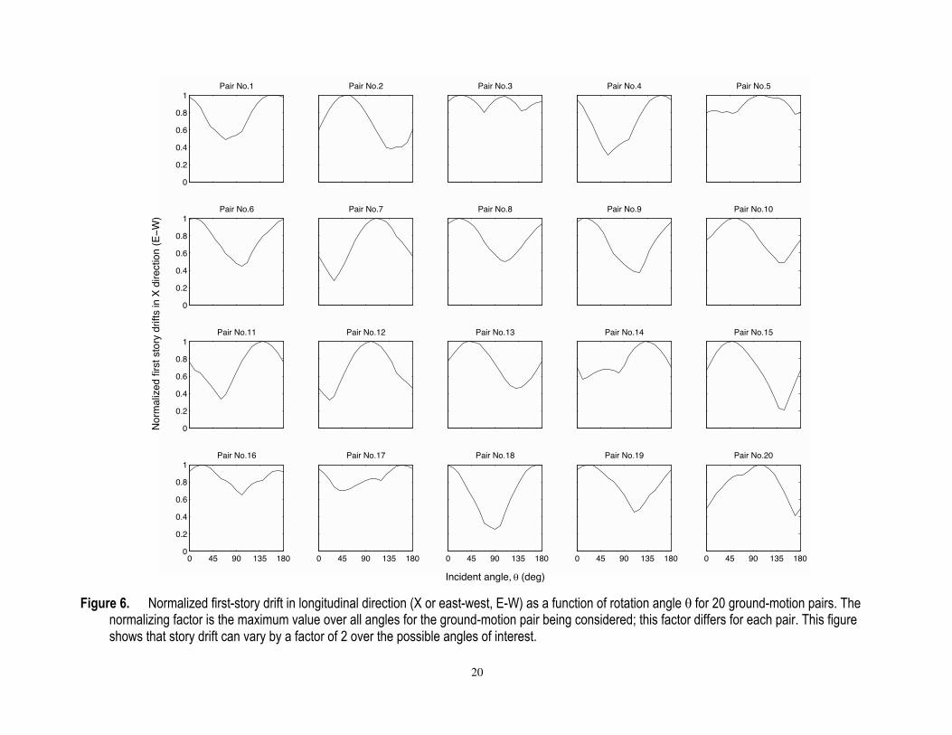
spectra rotated through all angles from 0 through 180 with a 5 interval. ............................. 19 6. Normalized first-story drift in longitudinal direction (X or east-west, E-W) as a function of

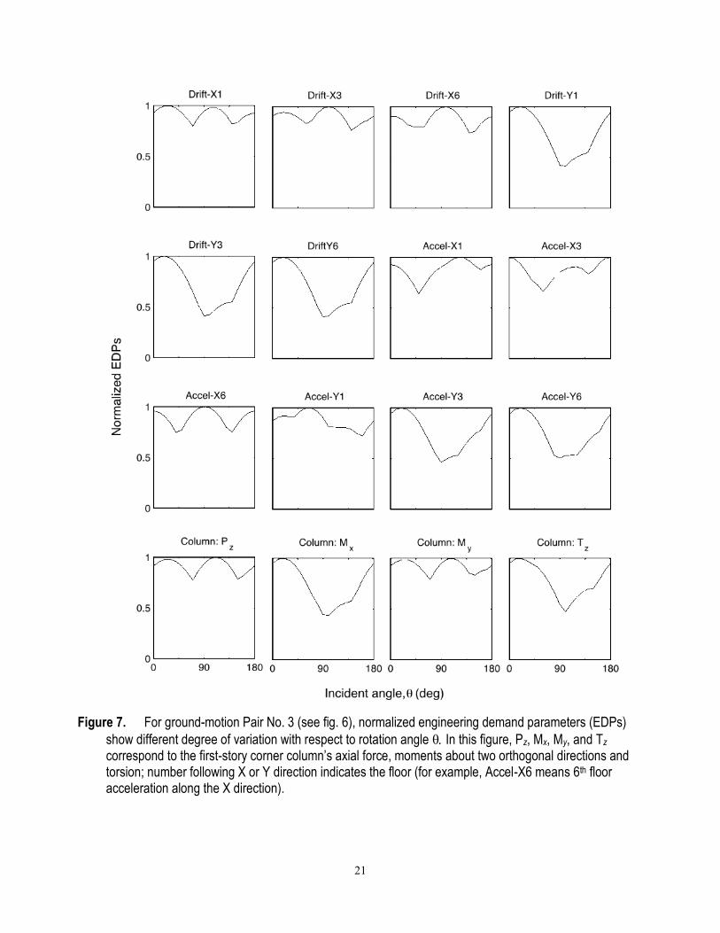
rotation angle θ for 20 ground-motion pairs. ............................................................................ 20 7. For ground-motion Pair No. 3, normalized engineering demand parameters (EDPs) show

different degree of variation with respect to rotation angle θ In this figure, Pz, Mx, My, and Tz correspond to the first-story corner column’s axial force, moments about two orthogonal directions and torsion; number following X or Y direction indicates the floor (for example, Accel-X6 means 6th floor acceleration along the X direction). .................................................. 21

8. Story-drift profiles in longitudinal (X or east-west, E-W) direction for 20 ground-motion pairs

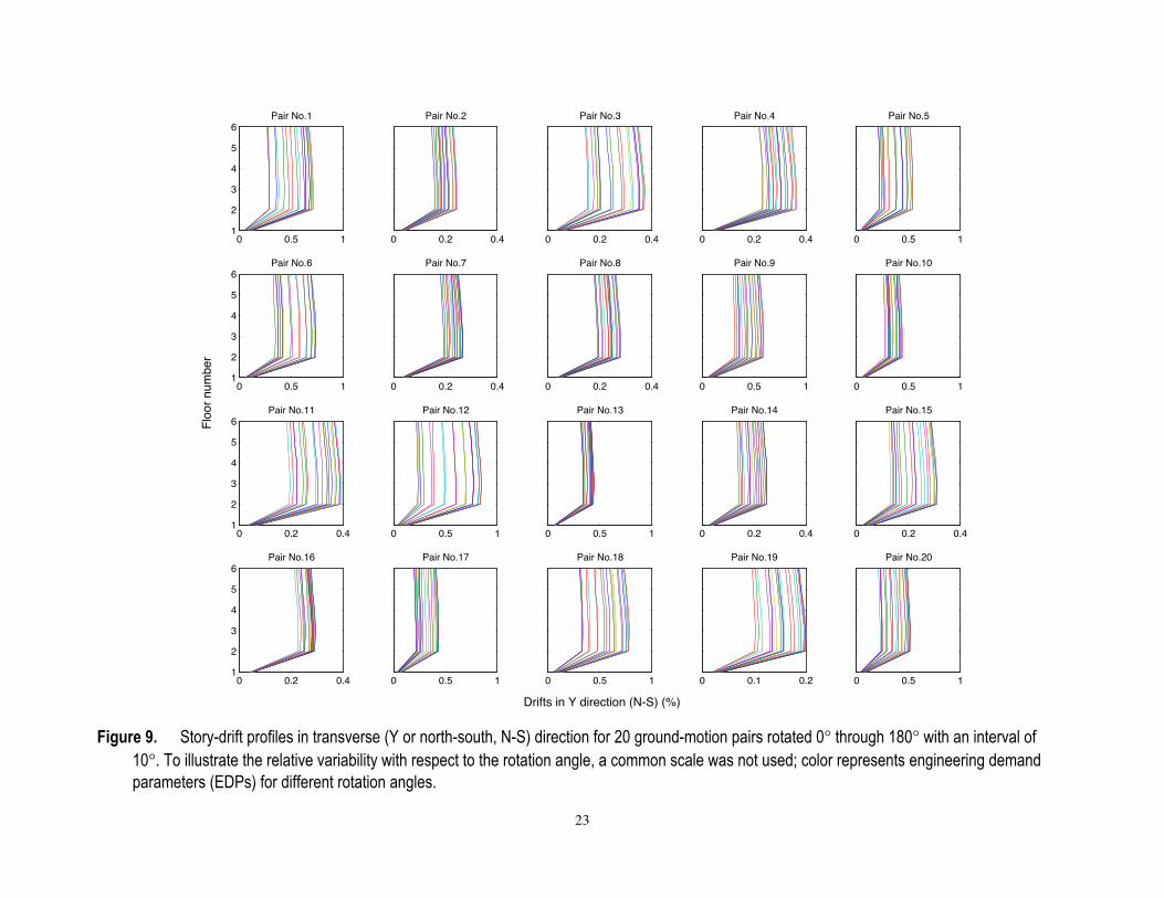
rotated 0 through 180 with an interval of 10. ....................................................................... 22 9. Story-drift profiles in transverse (Y or north-south, N-S) direction for 20 ground-motion

pairs rotated 0 through 180 with an interval of 10. .............................................................. 23

iv

10. Story-drift profiles in transverse (X or east-west, E-W) direction. ............................................. 24 11. Story-drift profiles in transverse (Y or north-south, N-S) direction. ........................................... 25 12. Histogram of 1,000 randomly obtained realizations of first-story drift in X or east west (E-

W) direction. ............................................................................................................................. 26 13. Histogram of 1,000 randomly obtained realizations of first-story drift in Y or north-south (N-

S) direction. ............................................................................................................................. 27 14. For a given pair of ground motion and a given value of first-story drifts in X or east-west (E-

W) direction, the probability of observing an engineering demand parameter (EDP) value equal to or less than the given EDP value is shown based on 1,000 realizations. ................... 28

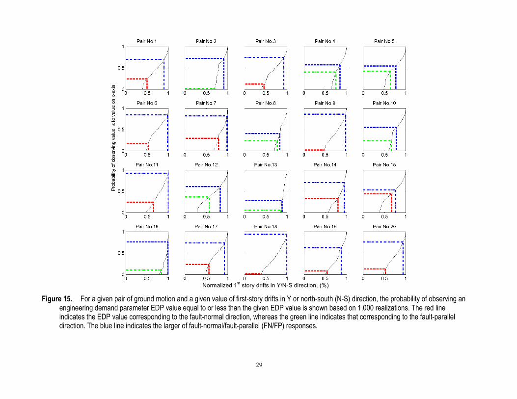
15. For a given pair of ground motion and a given value of first-story drifts in Y or north-south (N-S) direction, the probability of observing an engineering demand parameter EDP value equal to or less than the given EDP value is shown based on 1,000 realizations. ................... 29

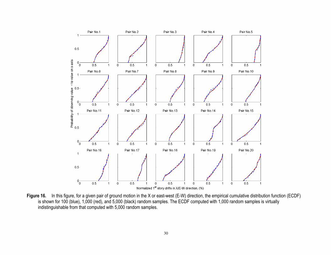
16. In this figure, for a given pair of ground motion in the X or east-west (E-W) direction, the empirical cumulative distribution function (ECDF) is shown for 100 (blue), 1,000 (red), and 5,000 (black) random samples. ................................................................................................ 30

Evaluation of Fault-Normal/Fault-Parallel Directions Rotated Ground Motions for Response History Analysis of an Instrumented Six-Story Building

By Erol Kalkan1 and Neal S. Kwong2

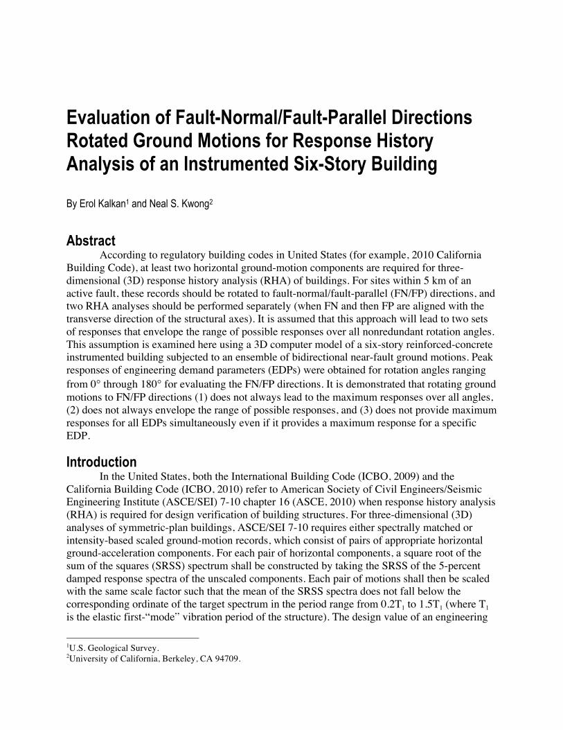
Abstract According to regulatory building codes in United States (for example, 2010 California

Building Code), at least two horizontal ground-motion components are required for three-dimensional (3D) response history analysis (RHA) of buildings. For sites within 5 km of an active fault, these records should be rotated to fault-normal/fault-parallel (FN/FP) directions, and two RHA analyses should be performed separately (when FN and then FP are aligned with the transverse direction of the structural axes). It is assumed that this approach will lead to two sets of responses that envelope the range of possible responses over all nonredundant rotation angles. This assumption is examined here using a 3D computer model of a six-story reinforced-concrete instrumented building subjected to an ensemble of bidirectional near-fault ground motions. Peak responses of engineering demand parameters (EDPs) were obtained for rotation angles ranging from 0° through 180° for evaluating the FN/FP directions. It is demonstrated that rotating ground motions to FN/FP directions (1) does not always lead to the maximum responses over all angles, (2) does not always envelope the range of possible responses, and (3) does not provide maximum responses for all EDPs simultaneously even if it provides a maximum response for a specific EDP.

Introduction In the United States, both the International Building Code (ICBO, 2009) and the

California Building Code (ICBO, 2010) refer to American Society of Civil Engineers/Seismic Engineering Institute (ASCE/SEI) 7-10 chapter 16 (ASCE, 2010) when response history analysis (RHA) is required for design verification of building structures. For three-dimensional (3D) analyses of symmetric-plan buildings, ASCE/SEI 7-10 requires either spectrally matched or intensity-based scaled ground-motion records, which consist of pairs of appropriate horizontal ground-acceleration components. For each pair of horizontal components, a square root of the sum of the squares (SRSS) spectrum shall be constructed by taking the SRSS of the 5-percent damped response spectra of the unscaled components. Each pair of motions shall then be scaled with the same scale factor such that the mean of the SRSS spectra does not fall below the corresponding ordinate of the target spectrum in the period range from 0.2T1 to 1.5T1 (where T1 is the elastic first-“mode” vibration period of the structure). The design value of an engineering

1U.S. Geological Survey. 2University of California, Berkeley, CA 94709.

2

demand parameter (EDP)—member forces, member deformations, or story drifts—shall then be taken as the mean value of the EDP over seven (or more) ground motion pairs, or its maximum value over all ground motion pairs, if the system is analyzed for fewer than seven ground motion pairs. This procedure requires a minimum of three records.

As input for RHAs, strong-motion networks provide users with ground accelerations recorded in three orthogonal directions—two horizontal and one vertical. The sensors recording horizontal accelerations are often, but not always, oriented in the North-South (N-S) and East-West (E-W) directions. These records with station-specific orientations are referred to as “as-recorded” ground motions. If the recording instrument had been installed in a different orientation about the vertical axis than the N-S and E-W directions, and the corresponding pair of ground motions was of interest, then a two-dimensional rotation transformation can be applied to the as-recorded motion. Because the instrument could have been installed at any angle, the rotated versions are possible realizations.

Although the as-recorded pair of ground motion may be applied to the structural axes corresponding to the structure’s transverse and longitudional directions, there is no reason why the pair should not be applied to any other axes rotated about the structural vertical axis. Equivalently, there is no reason why rotated versions should not be applied to the structural axes. Which angle, then, should one select for RHA remains a question in earthquake engineering practice.

This notion of rotating ground-motion pairs has been studied previously in various contexts. According to Penzien and Watabe (1975), the principal axis of a pair of ground motions is the angle or axis at which the two horizontal components are uncorrelated. Using this idea of principal axis, the effects of seismic rotation angle, defined as the angle between the principal axes of the ground-motion pair and the structural axes on which structural response was investigated (Fernandez-Davilla and others, 2000; MacRae and Matteis, 2000; Tezcan and Alhan, 2001; Khoshnoudian and Poursha, 2004; Rigato and Medina, 2007). A formula for deriving the angle that yields the peak elastic response over all possible nonredundant angles, called θcritical (or θcr), was proposed by Wilson (1995). Other researchers have improved on the closed-form solution of Wilson (1995) by accounting for the statistical correlation of horizontal components of ground motion in an explicit way (Lopez and Tores, 1997; Lopez and others, 2000). The Wilson (1995) formula is, however, based on concepts from response spectrum analysis—an approximate procedure used to estimate structural responses in the linear-elastic domain. Focusing on linear-elastic multi-degree-of-freedom symmetric and asymmetric structures, Athanatopoulou (2004) investigated the effect of the rotation angle on structural response using RHAs and provided formulas for determining the response at any rotation angle, given the response histories for two orthogonal orientations. Athanatopoulou (2004) also concluded that the critical angle corresponding to peak response over all angles varies not only with the ground-motion pair under consideration but with the response quantity of interest as well. However, no explanation was provided for the latter observation.

According to section 1615A.1.25 of the California Building Code (ICBO, 2010), at sites within 3 miles (5 kilometers, km) of the active fault that dominates the earthquake hazard, each pair of ground-motion components shall be rotated to the fault-normal and fault-parallel (FN/FP) directions (also called the strike-normal and strike-parallel directions) for 3D RHAs. It is believed that the angle corresponding to the FN/FP directions will lead to the most critical structural response. This assumption is based on the fact that, in the proximity of an active fault system, ground motions are significantly affected by the faulting mechanism, direction of rupture

3

propagation relative to the site, as well as the possible static deformation of the ground surface associated with fling-step effects (Kalkan and Kunnath, 2006); these near-source effects cause most of the seismic energy from the rupture to arrive in a single coherent long-period pulse of motion in the FN/FP directions (Kalkan and Kunnath, 2007; 2008). Thus, rotating ground-motion pairs to FN/FP directions is assumed to be a conservative approach appropriate for design verification of new structures or performance evaluation of existing structures.

Using a 3D structural model of an instrumented building and an ensemble of near-fault ground-motion records, this study systematically evaluates whether FN/FP directions rotated ground motions lead to conservative estimates of EDPs from RHAs.

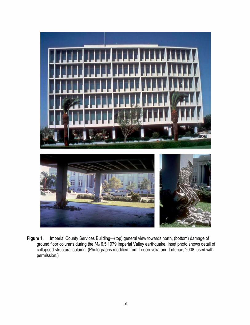
Description of Structural System and Computer Model The testbed system used is a 3D computer model of the former Imperial County Services

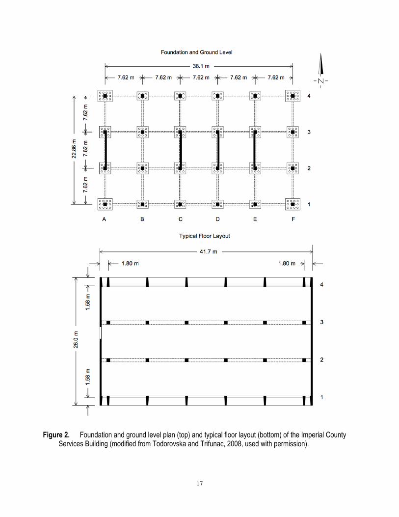
Building in El Centro, California. This relatively symmetrical building had an open first story and five occupied stories (fig. 1). Designed in 1968, its vertical load-carrying system consisted of 12.7-centimeter (5-inch) thick slabs of reinforced concrete (RC) supported by RC pan joists, which in turn are supported by RC frames spanning in the orthogonal direction. Figure 2 shows the foundation and typical floor layouts. Lateral resistance of all levels in the longitudinal (E-W) direction was provided by two exterior moment frames at column lines 1 and 4 and two interior moment frames on column lines 2 and 3. The lateral resistance in the transverse (N-S) direction was not continuous. At the ground floor level, it was provided by four short shear walls located along column lines A, C, D, and E and extending between column lines 2 and 3 only (figure 2 top). At the second floor and above, lateral (N-S) resistance was provided by two shear walls at the east and west ends of the building. This caused the building to appear top heavy with a soft first story as shown in figure 1 (Todorovska and Trifunac, 2008). The design strength of the concrete was 34.5 megapascals (MPa) (5 kilopound per square inch, ksi) for columns, 20.7 MPa (3 ksi) for the elements below ground level, and 27.6 MPa (4 ksi) elsewhere. All reinforcing steel was specified to be grade 40 (yield strength, Fy=276 MPa). The foundation system consisted of piles under each column with pile caps connected with RC beams (fig. 2 top).

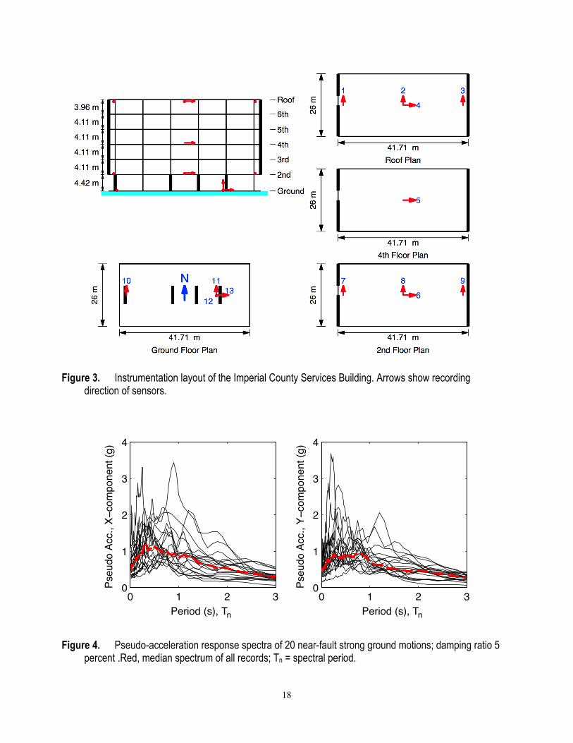
The building was instrumented in 1976 with 13 sensors at four levels of the building and 3 sensors at a reference free-field site. The sensors in the building measure horizontal accelerations at the ground floor, 2nd floor, 4th floor and roof; vertical acceleration was measured at the ground floor (fig. 3). The recorded motions of this building are available only for the Mw6.5 1979 Imperial Valley earthquake, during which this building was damaged. As a result, the building was subsequently demolished. The peak recorded accelerations during this earthquake were 0.34 g at the ground floor and 0.58 g at the roof level. This building is a rare case of an instrumented building severely damaged by an earthquake (Goel and Chadwell, 2007). Figure 1 (bottom) shows the concentration of damage in the ground-floor columns as a result of concrete spalling and buckling of reinforcing bars. The details about the design, recorded data and observed damage can be found in Kojic and others (1984).

The 3D computer model of this building was created using OpenSees (2010). Centerline dimensions were used in the element modeling, the composite action of floor slabs was not considered, and the columns were assumed to be fixed at the base level. For the response-history evaluations, masses were applied to frame models on the basis of the floor tributary area and were distributed proportionally to the floor nodes. The simulation models were calibrated to the response data (that is, floor accelerations) measured during the Imperial Valley earthquake so as to gain confidence in the computer model and analytical results of the comparative study.

4

Table 1 lists the linear-elastic periods of the first several modes, along with their modal participation and contribution factors (Chopra, 2007) for two orthogonal directions along the structural axes. The fundamental mode is primarily along the moment-frame (E-W direction) or X direction of the computer model. The irregularities in the N-S stiffness at the ground floor appear to have resulted in excessive torsional response and in significant coupling of the N-S and torsional excitations and responses. For the shear wall, or Y direction (N-S direction), the structure is not “first-mode dominated” as the modal contribution factor for the first mode in this direction is only 68 percent.

Ground-Motions Selected For this investigation, 20 near-fault strong-motion records, listed in table 2, were selected

from ten shallow crustal earthquakes compatible with the following scenario: • Moment magnitude: Mw=6.7±0.2 • Closest-fault distance: 0.1≤Rrup≤11 km • National Earthquake Hazards Reduction Program (NEHRP) soil type: C or D

Shown in figure 4 are the 5-percent damped-response spectra for the X and Y component of the as-recorded ground motions. Also shown is the median spectrum computed as the geometric mean of 20 response spectra in each direction. The median spectra show significantly large demands at the first and second mode of the building in both directions.

Methodology for Evaluation of Fault-Normal/Fault-Parallel Directions Restricting ourselves to the linear elastic version of the structural model, an attempt to

understand how structural responses vary with the rotation angle is made. Using the principle of superposition for a given response quantity, the response histories are computed for a range of rotation angles. Viewing the response as both a function of time and rotation angle enables us to better understand how the critical angle θcr, defined as the angle corresponding to the largest response over all angles, varies with both EDP and ground-motion pair.

For a given response quantity of interest and record pair, the FN/FP directions will correspond to two values. By comparing these two values with the responses at all other possible ground motion rotation angles, one can evaluate the level of conservatism in such directions; it means whether the FN/FP rotated ground motions provide an envelope of EDP. If obvious systematic benefits of the FN/FP orientations existed, they should be observable by repeating such comparisons for several EDPs and record pairs.

Even if no obvious trends are observed, one can still compare the FN/FP directions to no rotation at all. Rather than comparing the FN/FP directions to the as-recorded directions, however, the as-recorded direction may be viewed as an arbitrarily assigned orientation. As a result, one will be able to state the likelihood of the FN/FP responses being conservative instead of simply stating whether or not it was conservative.

If the rotation angle θ for a record pair was the only source of uncertainty and the probability distribution for θ was specified, then a conditional probability density function (PDF) for the structural response may be defined. In particular, if θ is uniformly distributed from 0° through 180°, then the PDF for the EDP may be estimated by (1) obtaining a random sample of n rotation angles based on the uniform distribution, (2) computing the EDP corresponding to each of the n angles, and (3) forming a histogram with the collection of EDP values (Wasserman, 2004). Equipped with an estimate of the EDP’s probability distribution, conditioned on a ground motion pair, one can approximately determine the probability of exceeding the FN/FP responses.

5

Low probabilities of exceedance would suggest that there is some merit in focusing our attention to the FN/FP directions.

Structural Response Variability with Rotation Angle According to the ASCE/SEI 7-10 provisions under Section 16.1.3.2, the horizontal

components are to be identically scaled such that the SRSS of the scaled response spectra in each horizontal direction exceed the target design spectrum by a factor of 1.3 over the period range of 0.2T1 to 1.5T1.

How will the SRSS spectrum change if the ground motion pair was rotated? By rotating each of the twenty record pairs in Table 2 from 0° to 180° with a 5° interval

in clock-wise, one can compute 36 alternative SRSS spectra. Figure 5 shows the maximum and minimum envelopes bounding such rotated versions of the SRSS response spectra of each ground-motion pair (no scaling is applied). In this figure, Drms refers to root mean square, a metric used to quantify the variability of spectral accelerations (Sa) with changing rotation angle. Drms is computed for each rotation angle over all spectral periods as:

(1)

where i refers to the ith spectral period and N is the total number of logarithmically spaced spectral periods. It is visually evident that the SRSS response spectrum does not vary much with rotation angle. The relatively small Drms values indicate that several rotated versions of the ground-motion pair can satisfy the ASCE/SEI criteria and yet provide structural responses that are different (as shown later). Figure 5 also implies that rotating ground motions has a marginal effect on the ground-motion-scaling factors computed for each ground-motion pair to satisfy the ASCE/SEI criteria.

How much variability is there in the elastic structural responses as the rotation angle is varied? Figure 6 addresses this question by showing the drifts in the longitudinal (E-W or X) direction for the first story as a function of the rotation angle for all records. To better understand the relative variability, each subplot was normalized by the maximum response over all angles. Maximum responses for individual ground-motion pairs were found to occur at different angles. With the exception of a few pairs, the first story drift in X direction can vary by a factor of 2 over the possible angles of interest. This is considered to be a large variation.

Although figure 6 indicates that the first story drift in X direction does not vary significantly with rotation angle for ground motion pair number three, the same statement cannot be made for other response quantities. Considering pair three, various other response quantities are shown as a function of rotation angle in figure 7. It is evident that peak values of other EDPs occur at different angles for the same record pair. Large variation for EDPs other than story drift is also observed. For example, the torsion for an arbitrarily selected column can vary by a factor of 2 over the possible angles.

To better quantify this variation with rotation angle, the coefficient of variation (COV) is computed using equation 2 for each ground motion pair and for each response quantity related to an arbitrarily selected corner column in the first story. These values are shown in table 3.

€

COV =

1n −1

(xi − x n−1

n

∑ )2

x (2)

6

The COV for the moment Mx is larger for ground-motion pair number one than for pair number two. The reverse is true, however, when the response quantity of interest is My instead. Here, the COV is larger for the second pair than for the first pair. These results demonstrate that one must consider both the response quantity of interest and the ground-motion characteristics when attempting to predict the variability with respect to rotation angle in advance.

The fact that the variability depends on both the response quantity and ground-motion pair can also be observed in figures 8 and 9, where the height-wise distribution of story drifts over several angles is shown. To illustrate the variability in the responses within each pair, a common scale was not used for the drift axis. The variability is significantly large for some ground-motion pairs (for example, pair nos. 12, 15, 18), as compared to smaller variability observed for pair nos. 3, 16, and 17 for the story drift in the X direction. For the 5th pair of ground motion in figure 8, the drift in the second story varies much more than the drift in the sixth story, indicating that higher-mode effects, contributing to the response with larger demands at upper stories, become more pronounced only at certain angles. These results also confirm the fact that θcr varies with ground motion and with response quantity of interest. This is because θcr is a quantity that is highly dependent on the complete response history of the EDP. As a result, predicting θcr is difficult.

Evaluation of Fault-Normal/Fault-Parallel Directions Rotated Ground Motions

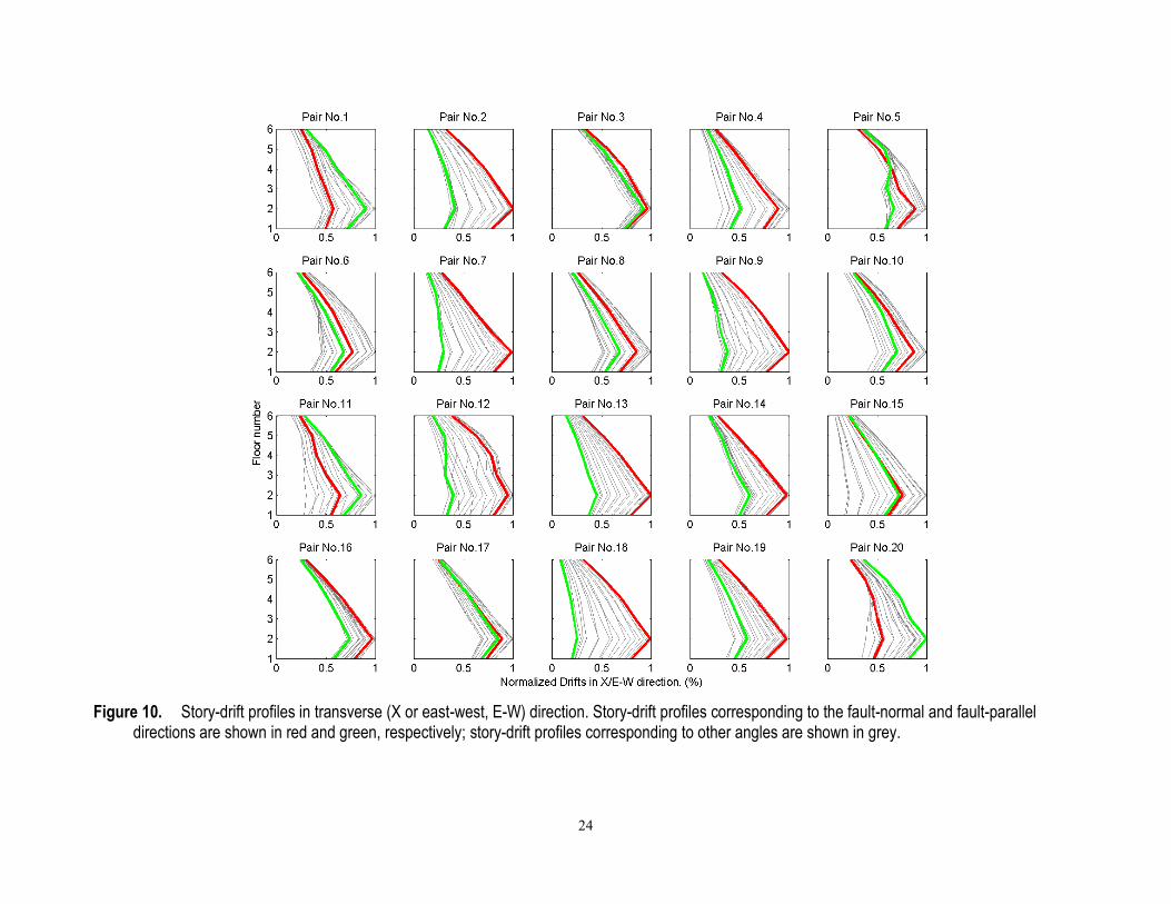
To evaluate the usefulness of rotating a record pair to the FN/FP directions, the EDPs corresponding to the FN/FP directions are compared against those corresponding to all other directions. To limit the computations to a reasonable size, each as-recorded pair is rotated clock-wise by increments of 10° before the EDPs are calculated. As a result, the two FN/FP sets of responses are compared against 19 other sets.

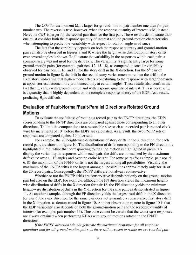
For example, the 20 height-wise distributions of story drifts in the X direction, for each record pair, are shown in figure 10. The distribution of drifts corresponding to the FN direction is highlighted in red, while that corresponding to the FP direction is highlighted in green. To display the variability in responses within each pair, the drifts are normalized by the maximum drift value over all 19 angles and over the entire height. For some pairs (for example, pair nos. 5, 6, 8), the maximum of the FN/FP drifts is not the largest among all possibilities. Visually, the maximum of the FN/FP drifts is the largest among all possibilities approximately only for 10 of the 20 record pairs. Consequently, the FN/FP drifts are not always conservative.

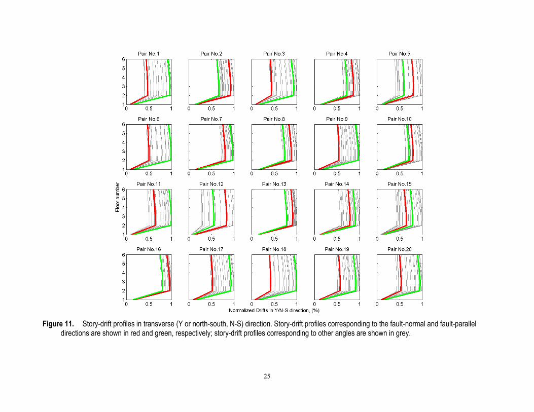
Whether or not the FN/FP drifts are conservative depends not only on the ground-motion pair but also on the EDP. For example, although the FN direction yields the maximum height-wise distribution of drifts in the X direction for pair 18, the FN direction yields the minimum height-wise distribution of drifts in the Y direction for the same pair, as demonstrated in figure 11. As another example, although the FP direction yields the largest roof drift in the X direction for pair 5, the same direction for the same pair does not guarantee a conservative first story drift in the X direction, as demonstrated in figure 10. Another observation to note in figure 10 is that the EDP variability also depends on both the ground-motion pair and the response quantity of interest (for example, pair number 13). Thus, one cannot be certain that the worst-case responses are always obtained when performing RHAs with ground motions rotated to the FN/FP directions.

If the FN/FP directions do not generate the maximum responses for all response quantities and for all ground-motion pairs, is there still a reason to rotate an as-recorded pair

7

prior to performing response history analyses? To address this issue, the FN/FP directions rotated ground motions are evaluated from a statistical viewpoint. Suppose the only source of aleatoric uncertainty in responses is due to uncertainty in the orientation, or rotation angle, of the ground-motion pair. In other words, given the structural model and ground motion pair, the EDP will have a probability distribution that is directly related to the probability distribution for the rotation angle. This conditional distribution for the EDP can serve as a benchmark to evaluate the usefulness in rotating as-recorded ground motions to the FN/FP directions.

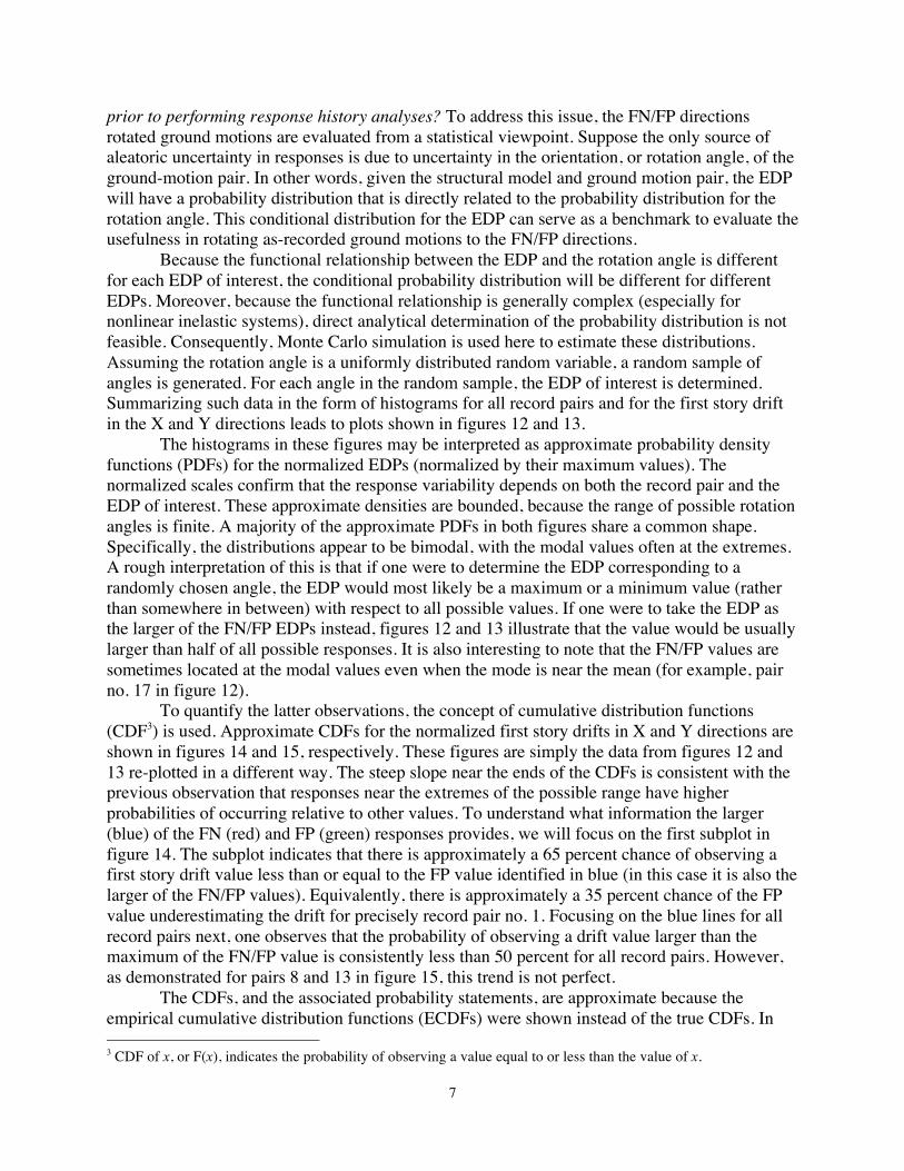
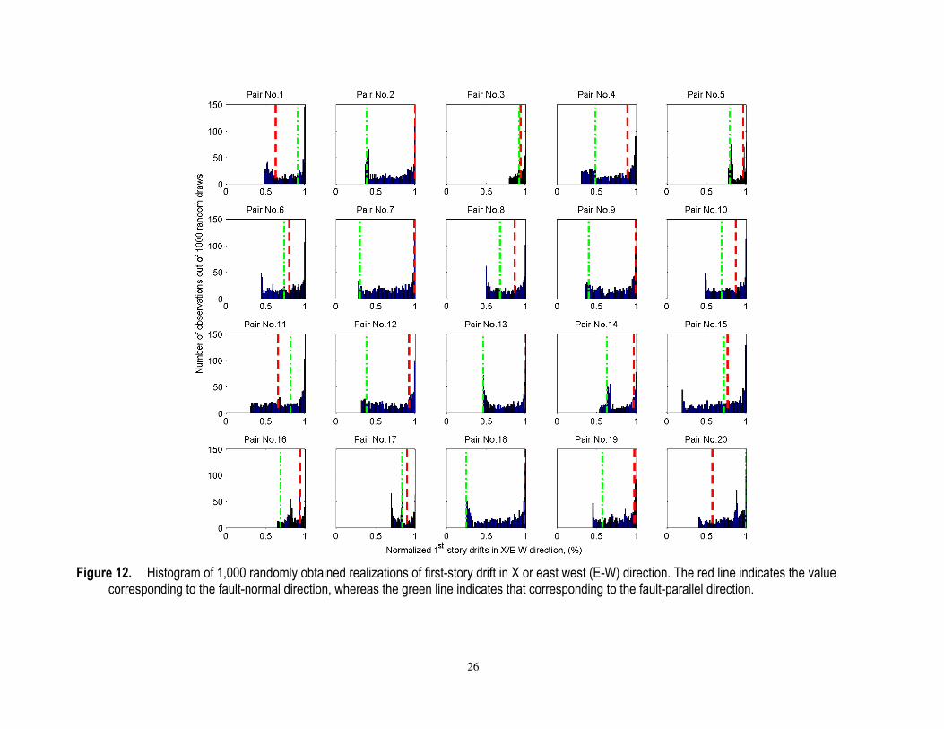
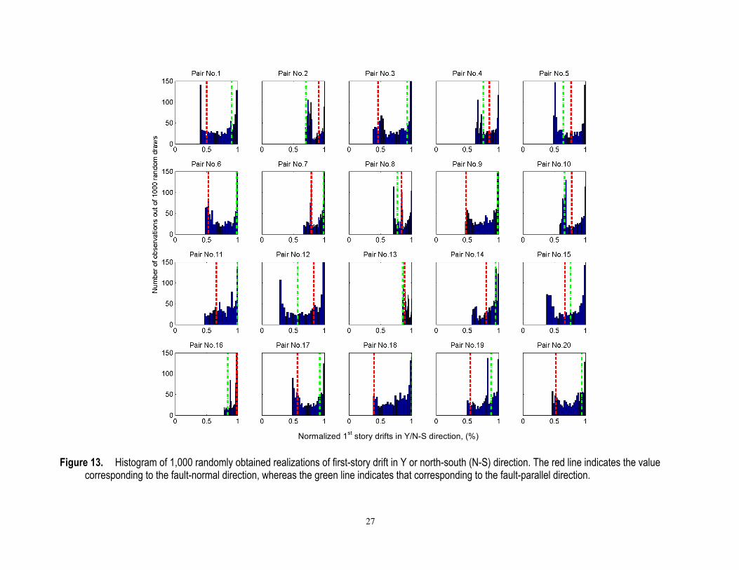
Because the functional relationship between the EDP and the rotation angle is different for each EDP of interest, the conditional probability distribution will be different for different EDPs. Moreover, because the functional relationship is generally complex (especially for nonlinear inelastic systems), direct analytical determination of the probability distribution is not feasible. Consequently, Monte Carlo simulation is used here to estimate these distributions. Assuming the rotation angle is a uniformly distributed random variable, a random sample of angles is generated. For each angle in the random sample, the EDP of interest is determined. Summarizing such data in the form of histograms for all record pairs and for the first story drift in the X and Y directions leads to plots shown in figures 12 and 13.

The histograms in these figures may be interpreted as approximate probability density functions (PDFs) for the normalized EDPs (normalized by their maximum values). The normalized scales confirm that the response variability depends on both the record pair and the EDP of interest. These approximate densities are bounded, because the range of possible rotation angles is finite. A majority of the approximate PDFs in both figures share a common shape. Specifically, the distributions appear to be bimodal, with the modal values often at the extremes. A rough interpretation of this is that if one were to determine the EDP corresponding to a randomly chosen angle, the EDP would most likely be a maximum or a minimum value (rather than somewhere in between) with respect to all possible values. If one were to take the EDP as the larger of the FN/FP EDPs instead, figures 12 and 13 illustrate that the value would be usually larger than half of all possible responses. It is also interesting to note that the FN/FP values are sometimes located at the modal values even when the mode is near the mean (for example, pair no. 17 in figure 12).

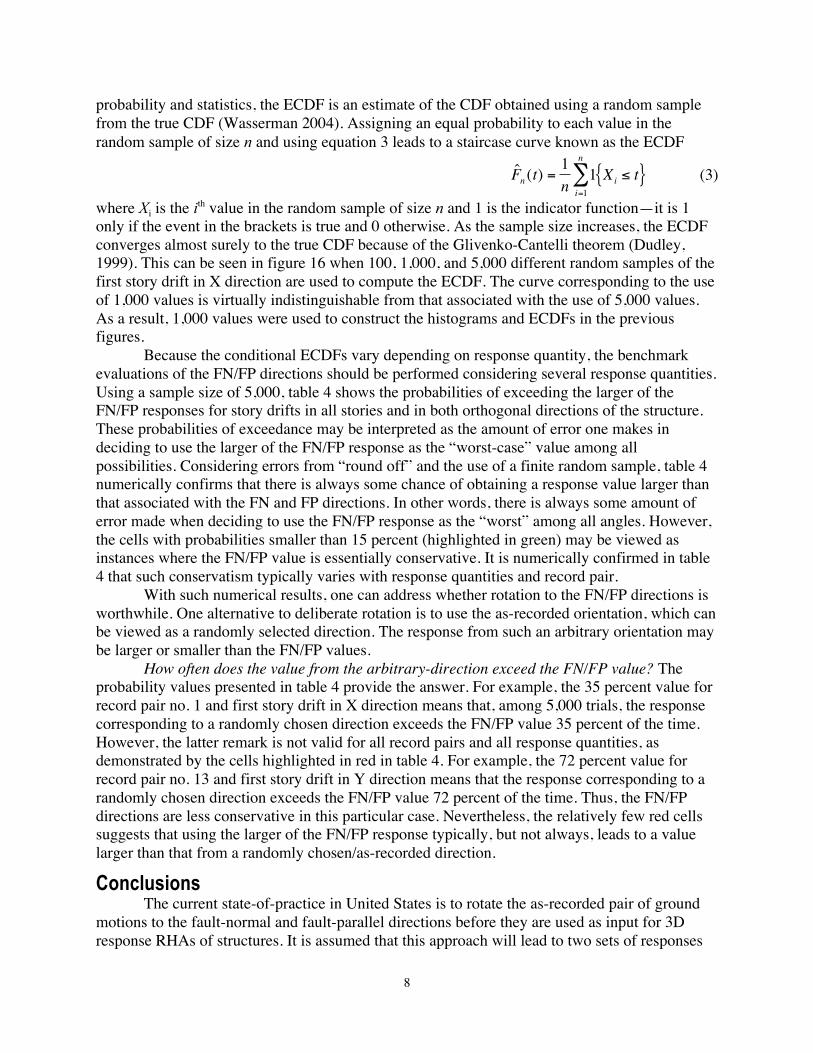
To quantify the latter observations, the concept of cumulative distribution functions (CDF3) is used. Approximate CDFs for the normalized first story drifts in X and Y directions are shown in figures 14 and 15, respectively. These figures are simply the data from figures 12 and 13 re-plotted in a different way. The steep slope near the ends of the CDFs is consistent with the previous observation that responses near the extremes of the possible range have higher probabilities of occurring relative to other values. To understand what information the larger (blue) of the FN (red) and FP (green) responses provides, we will focus on the first subplot in figure 14. The subplot indicates that there is approximately a 65 percent chance of observing a first story drift value less than or equal to the FP value identified in blue (in this case it is also the larger of the FN/FP values). Equivalently, there is approximately a 35 percent chance of the FP value underestimating the drift for precisely record pair no. 1. Focusing on the blue lines for all record pairs next, one observes that the probability of observing a drift value larger than the maximum of the FN/FP value is consistently less than 50 percent for all record pairs. However, as demonstrated for pairs 8 and 13 in figure 15, this trend is not perfect.

The CDFs, and the associated probability statements, are approximate because the empirical cumulative distribution functions (ECDFs) were shown instead of the true CDFs. In 3 CDF of x, or F(x), indicates the probability of observing a value equal to or less than the value of x.

8

probability and statistics, the ECDF is an estimate of the CDF obtained using a random sample from the true CDF (Wasserman 2004). Assigning an equal probability to each value in the random sample of size n and using equation 3 leads to a staircase curve known as the ECDF

€

ˆ F n (t) =1n

1 Xi ≤ t{ }i=1

n

∑ (3)

where Xi is the ith value in the random sample of size n and 1 is the indicator function—it is 1 only if the event in the brackets is true and 0 otherwise. As the sample size increases, the ECDF converges almost surely to the true CDF because of the Glivenko-Cantelli theorem (Dudley, 1999). This can be seen in figure 16 when 100, 1,000, and 5,000 different random samples of the first story drift in X direction are used to compute the ECDF. The curve corresponding to the use of 1,000 values is virtually indistinguishable from that associated with the use of 5,000 values. As a result, 1,000 values were used to construct the histograms and ECDFs in the previous figures.

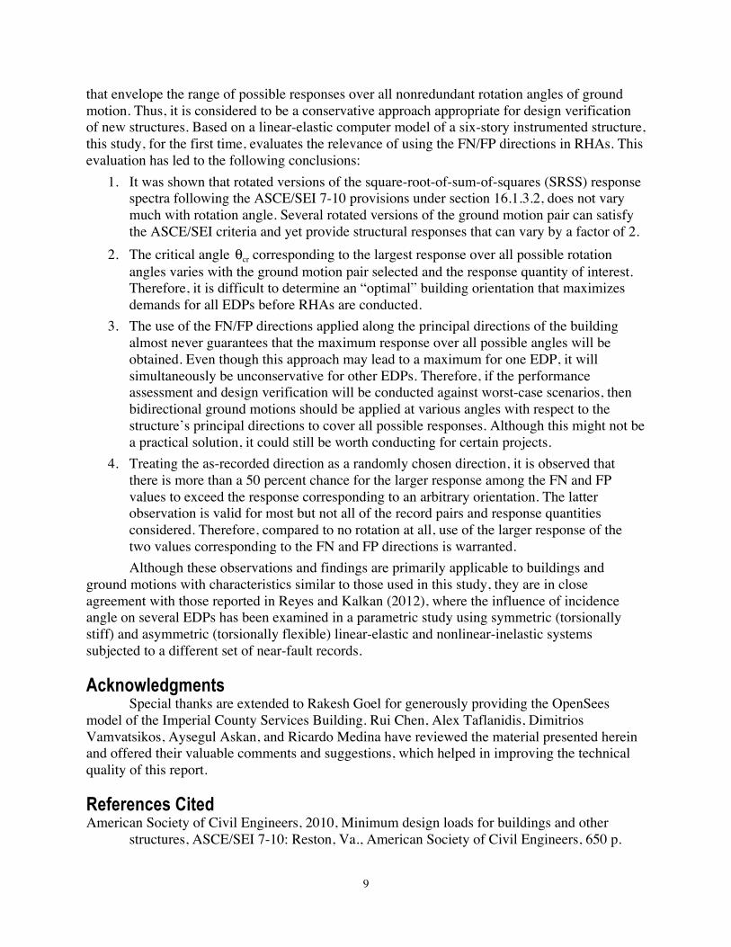
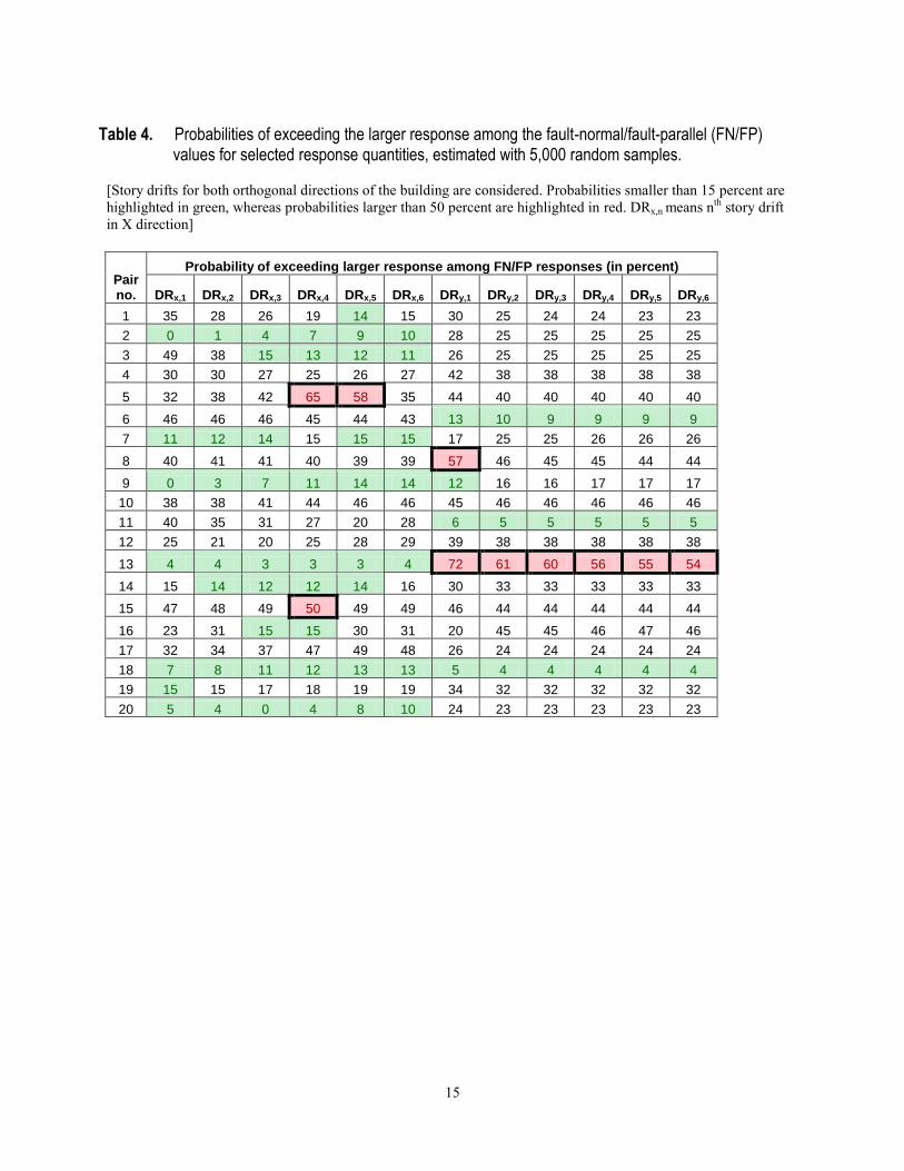
Because the conditional ECDFs vary depending on response quantity, the benchmark evaluations of the FN/FP directions should be performed considering several response quantities. Using a sample size of 5,000, table 4 shows the probabilities of exceeding the larger of the FN/FP responses for story drifts in all stories and in both orthogonal directions of the structure. These probabilities of exceedance may be interpreted as the amount of error one makes in deciding to use the larger of the FN/FP response as the “worst-case” value among all possibilities. Considering errors from “round off” and the use of a finite random sample, table 4 numerically confirms that there is always some chance of obtaining a response value larger than that associated with the FN and FP directions. In other words, there is always some amount of error made when deciding to use the FN/FP response as the “worst” among all angles. However, the cells with probabilities smaller than 15 percent (highlighted in green) may be viewed as instances where the FN/FP value is essentially conservative. It is numerically confirmed in table 4 that such conservatism typically varies with response quantities and record pair.

With such numerical results, one can address whether rotation to the FN/FP directions is worthwhile. One alternative to deliberate rotation is to use the as-recorded orientation, which can be viewed as a randomly selected direction. The response from such an arbitrary orientation may be larger or smaller than the FN/FP values.

How often does the value from the arbitrary-direction exceed the FN/FP value? The probability values presented in table 4 provide the answer. For example, the 35 percent value for record pair no. 1 and first story drift in X direction means that, among 5,000 trials, the response corresponding to a randomly chosen direction exceeds the FN/FP value 35 percent of the time. However, the latter remark is not valid for all record pairs and all response quantities, as demonstrated by the cells highlighted in red in table 4. For example, the 72 percent value for record pair no. 13 and first story drift in Y direction means that the response corresponding to a randomly chosen direction exceeds the FN/FP value 72 percent of the time. Thus, the FN/FP directions are less conservative in this particular case. Nevertheless, the relatively few red cells suggests that using the larger of the FN/FP response typically, but not always, leads to a value larger than that from a randomly chosen/as-recorded direction.

Conclusions The current state-of-practice in United States is to rotate the as-recorded pair of ground

motions to the fault-normal and fault-parallel directions before they are used as input for 3D response RHAs of structures. It is assumed that this approach will lead to two sets of responses

9

that envelope the range of possible responses over all nonredundant rotation angles of ground motion. Thus, it is considered to be a conservative approach appropriate for design verification of new structures. Based on a linear-elastic computer model of a six-story instrumented structure, this study, for the first time, evaluates the relevance of using the FN/FP directions in RHAs. This evaluation has led to the following conclusions:

1. It was shown that rotated versions of the square-root-of-sum-of-squares (SRSS) response spectra following the ASCE/SEI 7-10 provisions under section 16.1.3.2, does not vary much with rotation angle. Several rotated versions of the ground motion pair can satisfy the ASCE/SEI criteria and yet provide structural responses that can vary by a factor of 2.

2. The critical angle θcr corresponding to the largest response over all possible rotation angles varies with the ground motion pair selected and the response quantity of interest. Therefore, it is difficult to determine an “optimal” building orientation that maximizes demands for all EDPs before RHAs are conducted.

3. The use of the FN/FP directions applied along the principal directions of the building almost never guarantees that the maximum response over all possible angles will be obtained. Even though this approach may lead to a maximum for one EDP, it will simultaneously be unconservative for other EDPs. Therefore, if the performance assessment and design verification will be conducted against worst-case scenarios, then bidirectional ground motions should be applied at various angles with respect to the structure’s principal directions to cover all possible responses. Although this might not be a practical solution, it could still be worth conducting for certain projects.

4. Treating the as-recorded direction as a randomly chosen direction, it is observed that there is more than a 50 percent chance for the larger response among the FN and FP values to exceed the response corresponding to an arbitrary orientation. The latter observation is valid for most but not all of the record pairs and response quantities considered. Therefore, compared to no rotation at all, use of the larger response of the two values corresponding to the FN and FP directions is warranted. Although these observations and findings are primarily applicable to buildings and

ground motions with characteristics similar to those used in this study, they are in close agreement with those reported in Reyes and Kalkan (2012), where the influence of incidence angle on several EDPs has been examined in a parametric study using symmetric (torsionally stiff) and asymmetric (torsionally flexible) linear-elastic and nonlinear-inelastic systems subjected to a different set of near-fault records.

Acknowledgments Special thanks are extended to Rakesh Goel for generously providing the OpenSees

model of the Imperial County Services Building. Rui Chen, Alex Taflanidis, Dimitrios Vamvatsikos, Aysegul Askan, and Ricardo Medina have reviewed the material presented herein and offered their valuable comments and suggestions, which helped in improving the technical quality of this report.

References Cited American Society of Civil Engineers, 2010, Minimum design loads for buildings and other

structures, ASCE/SEI 7-10: Reston, Va., American Society of Civil Engineers, 650 p.

10

Athanatopoulou, A.M., 2004, Critical orientation of three correlated seismic components: Engineering Structures, v.27, p. 301–312.

Chopra, AK., 2007, Dynamics of structures—Theory and applications to equation engineering, 2nd ed.: Englewood Cliffs, N.J., Prentice Hall, 844 p.

Dudley, R.M., 1999, Uniform central lLimit theorems: Cambridge University Press, 452 p. Fernandez-Davila, I., Comeinetti, S., and Cruz, E.F., 2000, Considering the bi-directional effects

and the seismic angle variations in building design, in Proceedings of the 12th World Conference on Earthquake Engineering, Auckland, New Zealand: accessed March 20, 2012, at http://www.iitk.ac.in/nicee/wcee/article/0435.pdf.

Goel, R.K., and Chadwell, C., 2007, Evaluation of current nonlinear static procedures for concrete buildings using recorded strong-motion data: Sacramento, Calif., California Strong Motion Instrumentation Program, Data Interpretation Report.

International Conference of Building Officials (ICBO), 2009, International Building Code: Whittier, Calif., International Conference of Building Officials.

International Conference of Building Officials (ICBO), 2010, California Building Code, Whittier, Calif., International Conference of Building Officials.

Kalkan, E., and Kunnath, S.K., 2006, Effects of fling-step and forward directivity on the seismic response of buildings: Earthquake Spectra, v. 22, no. 2, p.367–390.

Kalkan, E., and Kunnath, S.K., 2007, Effective cyclic energy as a measure of seismic demand: Journal of Earthquake Engineering, v. 11, no. 5, p. 725–751.

Kalkan, E., and Kunnath, S.K., 2008, Relevance of absolute and relative energy content in seismic evaluation of structures: Advances in Structural Engineering, v. 11, no.1, p. 17–34.

Khoshnoudian, F., and Poursha, M., 2004, Responses of three dimensional buildings under bi-directional and unidirectional seismic excitations, in Proceedings of the 13th World Conference on Earthquake Engineering, Vancouver, Canada, August 1–6, 2004, accessed March 20, 2012, at http://www.iitk.ac.in/nicee/wcee/article/13_55.pdf.

Kojic, S., Trifunac, M.D., and Anderson, J.C., 1984, A post earthquake response analysis of the Imperial County Services Building in El Centro, Report CE 84-02: Los Angeles, Calif., University of Southern California, Department of Civil Engineering.

Lopez, O.A., and Torres, R., 1997, The critical angle of seismic incidence and structural response: Earthquake Engineering and Structural Dynamics, v. 26, p. 881–894.

Lopez, O.A., Chopra, A.K., and Hernandez, J.J., 2000, Critical response of structures to multicomponent earthquake excitation: Earthquake Engineering and Structural Dynamics, v. 29, p.1759–1778.

MacRae, G.A., and Mattheis, J., 2000, Three-dimensional steel building response to near-fault motions: American Society of Civil Engineers, Journal of Structural Engineering, v. 126, no.1, p.117–126.

OpenSees 2010, Open system for earthquake engineering simulation: OpenSees Web site accessed March 20, 2012, at http://opensees.berkeley.edu.

Penzien, J., and Watabe, M., 1975, Characteristics of 3-Dimensional earthquake ground motions, Earthquake Engineering and Structural Dynamics, v. 3, p. 365–373.

Reyes, J.C., and Kalkan, E., 2012, Significance of the ground motion rotation angle on nonlinear behavior of symmetric and asymmetric buildings in near fault sites, in Proceedings of the 9th International Conference on Urban Earthquake Engineering/4th Asia Conference on Earthquake Engineering, March 6–8, 2012: Tokyo, Japan, Tokyo Institute of Technology.

11

Rigato, A., and Medina, R.A., 2007, Influence of Angle of Incidence on the Seismic Demands for Inelastic Single-storey Structures Subjected to Bi-directional Ground Motions: Engineering Structures, v. 29, no.10, p. 2593-2601.

Tezcan, S.S., and Alhan, C., 2001, Parametric analysis of irregular structures under seismic loading according to the new Turkish Earthquake Code: Engineering Structures, v. 23, p. 600–609.

Todorovska, M.I., and Trifunac, M.D., 2008, Earthquake damage detection in the Imperial County Services Building III—Analysis of wave travel times via impulse response functions: Soil Dynamics and Earthquake Engineering, v. 28, no.5, p. 387–404.

Wasserman, L., 2004, All of statistics—A concise course in statistical inference: New York, N.Y., Springer, 461 p.

Wilson, E.L, and Suharwardy, I., 1995, A clarification of the orthogonal effects in a three-dimensional seismic analysis: Earthquake Spectra, v. 11, no.4, p.659–666.

12

Table 1. Linear-elastic dynamic properties of the Imperial County Services Building; the modal

participation () and modal contribution factors (MCF) are shown to illustrate how the first six modes contribute to the linear-elastic responses in two orthogonal directions.

Mode

Number (n) Period (s) Γn,x Γn,y MCF,x

(%) MCF,y

(%)

1 1.2 5.3 0.0 84.5 0.0

2 0.4 0.0 4.8 0.0 68.4

3 0.4 -1.9 0.0 10.5 0.0

4 0.3 0.0 -0.8 0.0 1.9

5 0.2 -1.0 0.0 3.0 0.0

6 0.2 -0.7 0.0 1.4 0.0

13

Table 2. Selected near-fault strong ground-motion records.

[Rrup, closest fault distance; VS30, average shear-wave velocity within 30 m of crust; PGA, peak ground acceleration;

PGV, peak ground velocity; PGD, peak ground displacement]

Fault-normal component

Fault-parallel component

Pair no.

Earthquake name Year Station name Mw

Rrup

(km)

VS30

(m/s)

PGA

(g) PGV

(cm/s) PGD (cm)

PGA

(g) PGV

(cm/s) PGD (cm)

1 Tabas, Iran 1978 Tabas 7.4 2.1 767 0.8 118 97 0.8 80 42

2 Imperial Valley, Calif.

1979 EC Meloland Overpass FF

6.5 0.1 186 0.4 115 40 0.3 27 15

3 Imperial Valley, Calif.

1979 El Centro Array #7

6.5 0.6 211 0.5 109 46 0.3 45 24

4 Superstition Hills, Calif.

1987 Parachute Test Site

6.5 1.0 349 0.4 107 51 0.3 50 22

5 Loma Prieta, Calif.

1989 Corralitos 6.9 3.9 462 0.5 45 14 0.5 42 7

6 Loma Prieta, Calif.

1989 LGPC 6.9 3.9 478 0.9 97 63 0.5 72 31

7 Erzincan, Turkey

1992 Erzincan 6.7 4.4 275 0.5 95 32 0.4 45 17

8 Northridge, Calif.

1994 Newhall - W Pico Canyon Rd

6.7 5.5 286 0.4 88 55 0.3 75 22

9 Northridge, Calif.

1994 Rinaldi Receiving Sta

6.7 6.5 282 0.9 167 29 0.4 63 21

10 Northridge, Calif.

1994 Sylmar - Converter Sta

6.7 5.4 251 0.6 130 54 0.8 93 53

11 Northridge, Calif.

1994 Sylmar - Converter Sta East

6.7 5.2 371 0.8 117 39 0.5 78 29

12 Northridge, Calif.

1994 Sylmar - Olive View Med FF

6.7 5.3 441 0.7 123 32 0.6 54 11

13 Kobe, Japan 1995 Takatori 6.9 1.5 256 0.7 170 45 0.6 63 23

14 Kocaeli, Turkey 1999 Yarimca 7.4 4.8 297 0.3 48 43 0.3 73 56

15 Chi-Chi, Taiwan 1999 TCU052 7.6 0.7 579 0.4 169 215 0.4 110 220

16 Chi-Chi, Taiwan 1999 TCU065 7.6 0.6 306 0.8 128 93 0.6 80 58

17 Chi-Chi, Taiwan 1999 TCU068 7.6 0.3 487 0.6 191 371 0.4 238 387

18 Chi-Chi, Taiwan 1999 TCU084 7.6 11.2 553 1.2 115 32 0.4 44 21

19 Chi-Chi, Taiwan 1999 TCU102 7.6 1.5 714 0.3 107 88 0.2 78 55

20 Duzce, Turkey 1999 Duzce 7.2 6.6 276 0.4 62 47 0.5 80 48

14

Table 3. Coefficient of variations (COV) for force (P) and moment (M or T) parameters along the X , Y , and Z directions of a first-story corner column (X = longitudinal, Y = transverse, Z = vertical direction in plan view).

[kips, kilopound per square inch; kip-in, kilopound per square inch-inch]

Pair no.

Coefficient of Variations for arbitrary 1st

-story corner column

Px (kips) Py (kips) Pz (kips) Mx (kip-in) My (kip-in) Tz (kip-in)

1 0.26 0.29 0.28 0.29 0.26 0.23

2 0.36 0.15 0.12 0.17 0.35 0.21

3 0.08 0.27 0.14 0.28 0.07 0.22

4 0.34 0.16 0.17 0.17 0.36 0.16

5 0.09 0.34 0.26 0.36 0.05 0.32

6 0.17 0.25 0.21 0.27 0.24 0.23

7 0.35 0.09 0.12 0.07 0.34 0.14

8 0.24 0.12 0.09 0.14 0.22 0.09

9 0.29 0.16 0.07 0.18 0.29 0.21

10 0.24 0.14 0.09 0.17 0.23 0.18

11 0.30 0.24 0.22 0.26 0.31 0.26

12 0.22 0.39 0.32 0.39 0.30 0.37

13 0.28 0.07 0.20 0.08 0.25 0.10

14 0.20 0.17 0.14 0.16 0.20 0.10

15 0.41 0.28 0.09 0.26 0.38 0.27

16 0.12 0.07 0.15 0.06 0.12 0.06

17 0.11 0.26 0.22 0.27 0.12 0.27

18 0.40 0.27 0.13 0.27 0.39 0.27

19 0.24 0.21 0.12 0.21 0.23 0.19

20 0.25 0.28 0.22 0.27 0.25 0.18

15

Table 4. Probabilities of exceeding the larger response among the fault-normal/fault-parallel (FN/FP) values for selected response quantities, estimated with 5,000 random samples.

[Story drifts for both orthogonal directions of the building are considered. Probabilities smaller than 15 percent are

highlighted in green, whereas probabilities larger than 50 percent are highlighted in red. DRx,n means nth

story drift

in X direction]

Pair no.

Probability of exceeding larger response among FN/FP responses (in percent)

DRx,1 DRx,2 DRx,3 DRx,4 DRx,5 DRx,6 DRy,1 DRy,2 DRy,3 DRy,4 DRy,5 DRy,6

1 35 28 26 19 14 15 30 25 24 24 23 23

2 0 1 4 7 9 10 28 25 25 25 25 25

3 49 38 15 13 12 11 26 25 25 25 25 25

4 30 30 27 25 26 27 42 38 38 38 38 38

5 32 38 42 65 58 35 44 40 40 40 40 40

6 46 46 46 45 44 43 13 10 9 9 9 9

7 11 12 14 15 15 15 17 25 25 26 26 26

8 40 41 41 40 39 39 57 46 45 45 44 44

9 0 3 7 11 14 14 12 16 16 17 17 17

10 38 38 41 44 46 46 45 46 46 46 46 46

11 40 35 31 27 20 28 6 5 5 5 5 5

12 25 21 20 25 28 29 39 38 38 38 38 38

13 4 4 3 3 3 4 72 61 60 56 55 54

14 15 14 12 12 14 16 30 33 33 33 33 33

15 47 48 49 50 49 49 46 44 44 44 44 44

16 23 31 15 15 30 31 20 45 45 46 47 46

17 32 34 37 47 49 48 26 24 24 24 24 24

18 7 8 11 12 13 13 5 4 4 4 4 4

19 15 15 17 18 19 19 34 32 32 32 32 32

20 5 4 0 4 8 10 24 23 23 23 23 23

16

Figure 1. Imperial County Services Building—(top) general view towards north, (bottom) damage of ground floor columns during the Mw 6.5 1979 Imperial Valley earthquake. Inset photo shows detail of collapsed structural column. (Photographs modified from Todorovska and Trifunac, 2008, used with permission.)

17

Figure 2. Foundation and ground level plan (top) and typical floor layout (bottom) of the Imperial County Services Building (modified from Todorovska and Trifunac, 2008, used with permission).

18

Figure 3. Instrumentation layout of the Imperial County Services Building. Arrows show recording direction of sensors.

Figure 4. Pseudo-acceleration response spectra of 20 near-fault strong ground motions; damping ratio 5 percent .Red, median spectrum of all records; Tn = spectral period.

! " # $!

"

#

$

%

&'()*+,-./0,12! " # $!

"

#

$

%

&'()*+,-./0,12

(a)

19

Figure 5. Maximum and minimum envelopes for square-root-of-sum-of-squares (SRSS) response spectra rotated through all angles from 0°

through 180° with a 5° interval. The root-mean-square (Drms) metric is shown for each horizontal pair of ground motion to indicate the degree of variation in rotated spectra; small values of Drms in all panels indicate that variation of spectral values by rotating ground-motion components is insignificant.

0

1

3

5Pair No.1

Drms=0.12

Pair No.2

Drms=0.12

Pair No.3

Drms=0.09

Pair No.4

Drms=0.14

Pair No.5

Drms=0.13

0

1

3

5Pair No.6

Drms=0.09

Pair No.7

Drms=0.12

Pair No.8

Drms=0.13

Pair No.9

Drms=0.11

Pair No.10

Drms=0.14

0

1

3

5Pair No.11

Drms=0.11

Pair No.12

Drms=0.11

Pair No.13

Drms=0.11

Pair No.14

Drms=0.15

Pair No.15

Drms=0.07

0 1 2 30

1

3

5Pair No.16

Drms=0.11

0 1 2 3

Pair No.17

Drms=0.12

0 1 2 3

Pair No.18

Drms=0.08

0 1 2 3

Pair No.19

Drms=0.11

0 1 2 3

Pair No.20

Drms=0.11

Period (s)

Spec

tral A

ccel

erat

ion,

(J)

20

Figure 6. Normalized first-story drift in longitudinal direction (X or east-west, E-W) as a function of rotation angle θ for 20 ground-motion pairs. The

normalizing factor is the maximum value over all angles for the ground-motion pair being considered; this factor differs for each pair. This figure shows that story drift can vary by a factor of 2 over the possible angles of interest.

!

!"#

!"$

!"%

!"&

'()*+,-."' ()*+,-."# ()*+,-."/ ()*+,-."$ ()*+,-."0

!

!"#

!"$

!"%

!"&

'()*+,-."% ()*+,-."1 ()*+,-."& ()*+,-."2 ()*+,-."'!

!

!"#

!"$

!"%

!"&

'()*+,-."'' ()*+,-."'# ()*+,-."'/ ()*+,-."'$ ()*+,-."'0

! $0 2! '/0 '&!!

!"#

!"$

!"%

!"&

'()*+,-."'%

! $0 2! '/0 '&!

()*+,-."'1

! $0 2! '/0 '&!

()*+,-."'&

! $0 2! '/0 '&!

()*+,-."'2

! $0 2! '/0 '&!

()*+,-."#!

!

345*6748,)49:7;,

21

Figure 7. For ground-motion Pair No. 3 (see fig. 6), normalized engineering demand parameters (EDPs)

show different degree of variation with respect to rotation angle θ In this figure, Pz, Mx, My, and Tz correspond to the first-story corner column’s axial force, moments about two orthogonal directions and torsion; number following X or Y direction indicates the floor (for example, Accel-X6 means 6th floor acceleration along the X direction).

22

Figure 8. Story-drift profiles in longitudinal (X or east-west, E-W) direction for 20 ground-motion pairs rotated 0° through 180° with an interval of

10°. To illustrate the relative variability with respect to the rotation angle, a common scale was not used; color represents EDPs for different rotation angles.

0 1 2 31

2

3

4

5

6Pair No.1

0 1 2

Pair No.2

0 0.5 1 1.5

Pair No.3

0 2 4

Pair No.4

0 0.5 1 1.5

Pair No.5

0 1 2 31

2

3

4

5

6Pair No.6

0 1 2 3

Pair No.7

0 1 2 3

Pair No.8

0 2 4 6

Pair No.9

0 2 4 6

Pair No.10

0 1 2 31

2

3

4

5

6Pair No.11

0 1 2 3

Pair No.12

0 5 10

Pair No.13

0 1 2

Pair No.14

0 2 4

Pair No.15

0 1 2 31

2

3

4

5

6Pair No.16

0 1 2 3

Pair No.17

0 2 4 6

Pair No.18

0 1 2 3

Pair No.19

0 1 2

Pair No.20

Drifts in X direction (E-W) (%)

Floo

r num

ber

23

Figure 9. Story-drift profiles in transverse (Y or north-south, N-S) direction for 20 ground-motion pairs rotated 0° through 180° with an interval of

10°. To illustrate the relative variability with respect to the rotation angle, a common scale was not used; color represents engineering demand parameters (EDPs) for different rotation angles.

0 0.5 11

2

3

4

5

6Pair No.1

0 0.2 0.4

Pair No.2

0 0.2 0.4

Pair No.3

0 0.2 0.4

Pair No.4

0 0.5 1

Pair No.5

0 0.5 11

2

3

4

5

6Pair No.6

0 0.2 0.4

Pair No.7

0 0.2 0.4

Pair No.8

0 0.5 1

Pair No.9

0 0.5 1

Pair No.10

0 0.2 0.41

2

3

4

5

6Pair No.11

0 0.5 1

Pair No.12

0 0.5 1

Pair No.13

0 0.2 0.4

Pair No.14

0 0.2 0.4

Pair No.15

0 0.2 0.41

2

3

4

5

6Pair No.16

0 0.5 1

Pair No.17

0 0.5 1

Pair No.18

0 0.1 0.2

Pair No.19

0 0.5 1

Pair No.20

Drifts in Y direction (N-S) (%)

Floo

r num

ber

24

Figure 10. Story-drift profiles in transverse (X or east-west, E-W) direction. Story-drift profiles corresponding to the fault-normal and fault-parallel directions are shown in red and green, respectively; story-drift profiles corresponding to other angles are shown in grey.

25

Figure 11. Story-drift profiles in transverse (Y or north-south, N-S) direction. Story-drift profiles corresponding to the fault-normal and fault-parallel directions are shown in red and green, respectively; story-drift profiles corresponding to other angles are shown in grey.

26

Figure 12. Histogram of 1,000 randomly obtained realizations of first-story drift in X or east west (E-W) direction. The red line indicates the value

corresponding to the fault-normal direction, whereas the green line indicates that corresponding to the fault-parallel direction.

27

Figure 13. Histogram of 1,000 randomly obtained realizations of first-story drift in Y or north-south (N-S) direction. The red line indicates the value corresponding to the fault-normal direction, whereas the green line indicates that corresponding to the fault-parallel direction.

Normalized 1st story drifts in Y/N-S direction, (%)

28

Figure 14. For a given pair of ground motion and a given value of first-story drifts in X or east-west (E-W) direction, the probability of observing an

engineering demand parameter (EDP) value equal to or less than the given EDP value is shown based on 1,000 realizations. The red line indicates the EDP value corresponding to the fault-normal direction, whereas the green line indicates that corresponding to the fault-parallel direction. The blue line indicates the larger of fault-normal/fault-parallel (FN/FP) responses.

29

Figure 15. For a given pair of ground motion and a given value of first-story drifts in Y or north-south (N-S) direction, the probability of observing an

engineering demand parameter EDP value equal to or less than the given EDP value is shown based on 1,000 realizations. The red line indicates the EDP value corresponding to the fault-normal direction, whereas the green line indicates that corresponding to the fault-parallel direction. The blue line indicates the larger of fault-normal/fault-parallel (FN/FP) responses.

Normalized 1st story drifts in Y/N-S direction, (%)

30

Figure 16. In this figure, for a given pair of ground motion in the X or east-west (E-W) direction, the empirical cumulative distribution function (ECDF)

is shown for 100 (blue), 1,000 (red), and 5,000 (black) random samples. The ECDF computed with 1,000 random samples is virtually indistinguishable from that computed with 5,000 random samples.