EXPLORING MOUNTAIN LION ECOLOGY IN TEXAS USING GENETIC

TECHNIQUES

A Thesis

by

JOSEPH DALE HOLBROOK

Submitted to the College of Graduate Studies

Texas A&M University-Kingsville

in partial fulfillment of the requirements for the degree of

MASTER OF SCIENCE

August 2011

Major Subject: Range and Wildlife Management

EXPLORING MOUNTAIN LION ECOLOGY IN TEXAS USING GENETIC

TECHNIQUES

A Thesis

by

JOSEPH DALE HOLBROOK

Approved as to style and content by:

_______________________________ ______________________________

Randall DeYoung, Ph.D. Michael Tewes, Ph.D.

(Co-Chairman of Committee) (Co-Chairman of Committee)

_______________________________

John Young, Ph.D.

(External Member)

____________________________

Scott Henke, Ph.D.

(Head of Department)

________________________________________________

Ambrose O. Anoruo, Ph.D.

(AVP & Dean, Research and Graduate Studies)

August 2011

iii

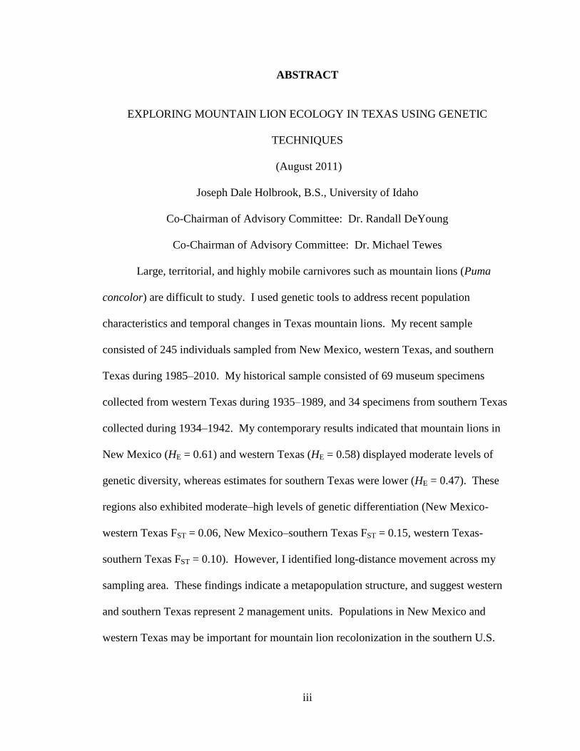
ABSTRACT

EXPLORING MOUNTAIN LION ECOLOGY IN TEXAS USING GENETIC

TECHNIQUES

(August 2011)

Joseph Dale Holbrook, B.S., University of Idaho

Co-Chairman of Advisory Committee: Dr. Randall DeYoung

Co-Chairman of Advisory Committee: Dr. Michael Tewes

Large, territorial, and highly mobile carnivores such as mountain lions (Puma

concolor) are difficult to study. I used genetic tools to address recent population

characteristics and temporal changes in Texas mountain lions. My recent sample

consisted of 245 individuals sampled from New Mexico, western Texas, and southern

Texas during 1985–2010. My historical sample consisted of 69 museum specimens

collected from western Texas during 1935–1989, and 34 specimens from southern Texas

collected during 1934–1942. My contemporary results indicated that mountain lions in

New Mexico (HE = 0.61) and western Texas (HE = 0.58) displayed moderate levels of

genetic diversity, whereas estimates for southern Texas were lower (HE = 0.47). These

regions also exhibited moderate–high levels of genetic differentiation (New Mexico-

western Texas FST = 0.06, New Mexico–southern Texas FST = 0.15, western Texas-

southern Texas FST = 0.10). However, I identified long-distance movement across my

sampling area. These findings indicate a metapopulation structure, and suggest western

and southern Texas represent 2 management units. Populations in New Mexico and

western Texas may be important for mountain lion recolonization in the southern U.S.

iv

Comparisons including historical samples revealed a ≈10-20% decline in genetic

diversity for southern Texas over time, while diversity in western Texas has remained

stable. Genetic differentiation between western and southern Texas has increased 2.5

times, which is likely due to the temporal changes that have occurred within southern

Texas (temporal FST = 0.13) rather than western Texas (temporal FST = 0.02). Effective

size estimates indicated a lower historical population size in southern Texas relative to

western Texas, and that southern Texas has declined > 50% over time. Effective size in

western Texas has remained large and stable. My findings show substantial temporal

declines and changes have occurred in southern Texas. Future research exploring

reproduction and survival in southern Texas is essential. Management actions such as

monitoring and harvest reduction may be needed to ensure the persistence of mountain

lions in Texas. Overall, this study emphasizes the importance and utility of applying

genetic tools to assist wildlife management and conservation.

v

DEDICATION

This thesis is dedicated to my parents (Chris and Dale), sister (Nicole), and dog

(Chief). I would not be here today without their unmatched love, support, and

encouragement. I am sincerely blessed to call them family! I also dedicate this work to

my Grandpa (Marvin), a true woodsman. His love of the outdoors and wildlife has

carried over 2 generations, and has largely influenced my career path in wildlife science.

Thank you Grandpa, I love and miss you!

vi

ACKNOWLEDGMENTS

First, I thank the Lord for giving me the strength, persistence, and ability to

complete my Master’s degree. Next, I sincerely thank my advisory committee Drs Randy

DeYoung, Mike Tewes, and John Young for their considerable support throughout the

project. My major professors, Randy DeYoung and Mike Tewes, deserve special thanks

for providing valuable insight, opportunities, criticism, time and effort, and friendship

during my stay at Kingsville. I very much enjoyed working under their tutelage and

appreciated the flexibility they offered to explore my ideas.

My fellow graduate students and colleagues deserve many thanks for their

support, as well as providing an environment that made the transition much easier for us

out-of-staters. Special thanks go to the cat coalition for stimulating conversations

regarding felid and carnivore ecology - thank you Arturo Caso, Lon Grassman, Chad

Stasey, Jen Korn, and Sasha Carvajal. I also thank the genetics crew for 1) keeping the

lab fun and lively around the clock, 2) their support and criticism, and 3) many

discussions regarding the application of genetic tools to ecological questions. I

particularly acknowledge Kelly Corman, Amber Dunn, Carlos Lopez, Karla Logan,

Damon Williford, Renee Keleher, Aaron Foley, and Johanna Delgado Acevedo.

Furthermore, Dr. Fred Bryant and the Caesar Kleberg Wildlife Research Institute staff

deserve large thanks for their valuable and much appreciated support. Yolanda Ballard,

Jere Sepulveda, DeAnna Greer, Chris Reopelle, Sara Barrera, and Becky Trant offered

essential insight that helped me successfully complete my degree.

Finally, I thank the collaborators and funding sources that were imperative to the

success of this project. Thanks to Bill Applegate, Louis Harveson, The Museum of

vii

Southwestern Biology - Division of Genomic Resources, and Jimmy Rutledge for

providing tissue samples. I greatly thank the National Museum of Natural History, Texas

Tech University, Sul Ross State University, Field Museum of Natural History, and

Carnegie Museum of Natural History for allowing access to historical samples. Many

thanks to Greta Shuster for providing lab space for me to process historical samples. I

thank Eric Redeker for his assistance and insight regarding GIS applications. The

Houston Safari Club, Quail Unlimited, South Texas Chapter, and the Quail Coalition

deserve special thanks for valuable scholarship funds. All financial support for this

research was provided by the Texas Parks and Wildlife Department, which was

absolutely essential and greatly appreciated.

viii

TABLE OF CONTENTS

Page

ABSTRACT ....................................................................................................................... iii

DEDICATION .....................................................................................................................v

ACKNOWLEDGMENTS ................................................................................................. vi

TABLE OF CONTENTS ................................................................................................. viii

LIST OF TABLES ............................................................................................................. xi

LIST OF FIGURES .......................................................................................................... xii

CHAPTER I: MOUNTAIN LIONS IN THE UNITED STATES AND TEXAS .............1

Overview ..................................................................................................................1

Ecology and demographics in Texas .......................................................................4

Literature cited .........................................................................................................6

CHAPTER II: GENETIC DIVERSITY, POPULATION GENETIC STRUCTURE,

AND MOVEMENTS OF MOUNTAIN LIONS (PUMA CONCOLOR) IN

TEXAS .......................................................................................................11

Abstract ..................................................................................................................11

Introduction ............................................................................................................12

Materials and methods ...........................................................................................14

Study area...................................................................................................14

Sample collection and DNA analysis ........................................................16

Genetic diversity and Hardy-Weinberg equilibrium..................................17

Genetic associations with distance.............................................................17

Genetic structure ........................................................................................18

ix

Assigning origin to dispersers ....................................................................20

Results ....................................................................................................................22

Genetic data ...............................................................................................22

Genetic associations with distance.............................................................22

Genetic structure ........................................................................................25

Assigning origin to dispersers ....................................................................34

Discussion ..............................................................................................................36

Acknowledgments..................................................................................................42

Literature cited .......................................................................................................42

CHAPTER III: DEMOGRAPHIC HISTORY OF AN ELUSIVE CARNIVORE: USING

MUSEUMS TO INFORM MANAGEMENT .........................................52

Summary ................................................................................................................52

Introduction ............................................................................................................53

Materials and methods ...........................................................................................57

Data analysis ..............................................................................................59

Results ....................................................................................................................62

Genetic diversity and differentiation .........................................................63

Effective population size............................................................................66

Discussion ..............................................................................................................69

Conservation and management implications .............................................73

Acknowledgements ................................................................................................75

References ..............................................................................................................75

APPENDICES ...................................................................................................................84

x

Appendix S1. Museum samples from Texas used in analyses .............................84

VITA ..................................................................................................................................86

xi

LIST OF TABLES

Table Page

2.1 Mountain lion genetic diversity in Texas and New Mexico ................................23

2.2 Pairwise estimates of FST for Texas and New Mexico mountain lions ................27

2.3 Genetic assignments for dispersers east of known populations ............................35

3.1 Genetic diversity per locus for Texas mountain lions ..........................................64

3.2 Allelic richness per locus for Texas mountain lions .............................................65

3.3 Variance effective population size (NeV) for Texas mountain lions .....................67

3.4 Effective number of breeders (Nb) for Texas mountain lions ...............................68

xii

LIST OF FIGURES

Figure Page

1.1 Mountain lion mortality reports in Texas ...............................................................3

2.1 Mountain lion sampling distribution throughout Texas and New Mexico ...........15

2.2 Relationship between genetic and Euclidean distance ..........................................24

2.3 Correlogram showing spatial genetic autocorrelation ..........................................26

2.4 Genetic clustering results from GENELAND ......................................................29

2.5 Genetic clustering results from BAPS ..................................................................30

2.6 The log probability of the data and ΔK from STRUCTURE ................................31

2.7 Ancestry proportions (q-values) from STRUCTURE ..........................................33

3.1 Temporal mountain lion sampling distribution throughout Texas .......................56

Chapter 1 of this thesis follows the format of the Journal of Wildlife Management.

1

CHAPTER I

MOUNTAIN LIONS IN THE UNITED STATES AND TEXAS

OVERVIEW

The mountain lion (Puma concolor) is a large, cryptic carnivore that occupies a

variety of habitats from northern Canada to the southern extent of South America

(Hornocker 1970, Hall 1981, Nowak 1991, Culver et al. 2000). Mountain lions are

mostly solitary (Hornocker 1969, 1970, Seidensticker et al.1973), exhibit a polygynous

mating system (Murphy 1998, Logan and Sweanor 2001), and occupy large territories

(10s–100s of km2; Seidensticker et al.1973, Ross and Jalkotzy 1992, Pierce et al. 1999,

Logan and Sweanor 2001). These large predators are highly mobile (Beier 1995, Ruth et

al. 1998), as revealed by dispersal distances up to 1,067 km (Thompson and Jenks 2005).

The behavioral and ecological characteristics of mountain lions have facilitated

contradictory social perceptions among humans. Many idealize mountain lions for their

charismatic qualities, whereas others are fearful and view them as direct competitors for

resources. Indeed, mountain lion-human conflicts have persisted for many years (Wade

et al. 1984).

Mountain lions have experienced persecution for centuries throughout much of

their range in the contiguous U.S. through recreational and bounty programs (i.e.,

trapping and hunting). The primary goal of these removal efforts was to minimize

depredation of livestock and big-game species (Doughty 1983, Wade et al. 1984, Logan

and Sweanor 2001). However, by the 1960s and 1970s most western U.S. states

regulated the harvest of mountain lions classifying them as game animals (Beausoleil et

2

al. 2008). This classification followed accomplishments in mountain lion research

identifying the biological roles they fulfill in ecosystems (Noss et al. 1996). The social

acceptance regarding unlimited take of a charismatic predator was also rapidly declining

by the 1970s (Russ 1996). The regulation of mountain lion harvest has contributed to

population stability throughout much of the western U.S. (e.g., Logan and Sweanor

2001), and created opportunity for re-expansion into their historical range.

However, mountain lion populations in Texas have sustained a restricted

distribution due to predator removal programs, bounties, and loss of habitat throughout

the 19th

and early 20th

century (Doughty 1983, Wade et al. 1984). Currently, Texas is the

only state in the U.S. where mountain lions are not classified as a game species, allowing

unregulated take with no mandatory inspection (Doughty 1983, Wade et al. 1984, Russ

1996). Young (2008) summarized harvest data spanning 1919–2006 from the U.S.

Department of Agriculture, Texas Division of Wildlife Services, which indicated a mean

of ~21 individuals taken per year and 2 substantial peaks in harvest during 1930–1938

and 1979–2004.

The unlimited harvest of mountain lions in Texas has led many to question the

viability of populations in the state. In response, the Texas Parks and Wildlife

Department (TPWD) began recording sightings and voluntary mortality reports from

various sources in 1982. The goal of this effort was to document relative changes in

mountain lion populations as well as distributional shifts in Texas. Recent (1980s–

2000s) mortality reports suggest that mountain lion populations are expanding (Figure

1.1; Sullins 2002). However, since 1970 (officially classified as non-game) there

3

Figure 1.1. The distribution of mountain lion mortalities reported in Texas, USA,

during 1983–2005. Reports were documented by the Texas Parks and Wildlife

Department.

4

has been no change in the status of mountain lions or harvest regulations and concerns of

over-harvest remain (Russ 1996). TPWD has sponsored several studies since 1982 to

better evaluate the status of mountain lions in Texas.

ECOLOGY AND DEMOGRAPHICS IN TEXAS

Mountain lions in Texas primarily select large prey species, such as mule deer

(Odocoileus hemionus) and white-tailed deer (Odocoileus virginianus), and supplement

their diet with a variety of other species (e.g., collared peccary [Tayassu tajacu],

livestock, porcupine [Erethizon dorsatum], nine-banded armadillo [Dasypus

novemcinctus], striped skunk [Mephitis mephitis]; McBride 1976, Leopold and Krausman

1986, Smith et al. 1986, Waid 1990). The age structure of mountain lions in Texas was

estimated from radio-telemetry studies, and is indicative of an exploited population where

a high proportion of individuals are in young (e.g., 24–48 months) age classes (McBride

1976, Smith et al. 1986, McBride and Ruth 1988, Waid 1990, Harveson et al. 1996).

Harveson et al. (1996) extrapolated density and home range estimates from previous

studies assuming an effective area size 1.5 times greater than the documented study area;

estimates ranged from 1.39–15 mountain lions/1,000 km2. Home range estimates ranged

from 59 km2–1,032 km

2 for females (Andersen 1983, Smith et al. 1986), and 207 km

2–

1,032 km2 for males (Andersen 1983, Smith et al. 1986).

Relatively recent mountain lion research has continued to address fundamental

ecological questions as well as explore the genetic properties of the southern and western

Texas populations. Harveson (1997) evaluated the ecology of a mountain lion population

in southern Texas and found that mean annual ranges were smaller for females (131.76

km2) than for males (503.48 km

2), and annual male-male and female-male range overlap

5

was extensive. Riparian habitats were preferred, while chaparral-dominant habitats were

avoided or used in proportion to available by both sexes. Subadult dispersal distances for

males (n = 4) ranged from 11.0–95.5 km and 6.3–23.1 km for females (n = 6; Harveson

1997). Mountain lions in southern Texas preferred preying on white-tailed deer,

exhibited a density of 0.59–0.74 individuals/100 km2, and survival of 0.81 (males) and

0.59 (females), respectively (Harveson 1997). Conclusions of this research suggested

high mortality coupled with low productivity of females may limit mountain lion

populations in southern Texas (Harveson 1997).

In another recent ecological study of mountain lions, Pittman et al. (2000)

examined a population occurring in western Texas. Male mountain lions exhibited larger

home ranges (348.6 km2) than that of females (205.9 km

2), and ~25% home range

overlap was documented among and between sexes (Pittman et al. 2000). Similar to

previous studies, fecal analyses indicated that mule deer and collared peccary were

preferred prey. Pittman et al. (2000) identified mountain lion density ranging from 0.26–

0.59 individuals/100 km2, and suggested that populations were limited by high male and

female mortality rates.

Lastly, 2 genetic studies were conducted in Texas addressing population genetic

structure of mountain lions (Walker et al. 2000, J. E. Janecka, Texas A&M University-

Kingsville, unpublished data). Walker et al. (2000) identified low levels of

heterozygosity within southern Texas (southern TX = 0.294) relative to the mountain lion

mean in North America (mean = 0.42, SE = 0.16; Culver et al. 2000). Populations in

southern and western Texas also exhibited reduced gene flow (Walker et al. 2000). More

localities were sampled in the most recent mountain lion study, however, results

6

generally supported Walker et al. (2000) conclusions; a genetic subdivision between

southern and western Texas and low levels of variation in southern Texas (J. E. Janecka,

Texas A&M University-Kingsville, unpublished data).

Previous research on mountain lions in Texas has provided an important

foundation of knowledge. However, essentially all studies have suffered from small

sample sizes, limited geographic extent, and short duration leaving many questions

unexplored. I employed genetic methods using harvested individuals (recently and

historically) to expand the knowledge of mountain lions in Texas, both spatially and

temporally. I addressed questions related to population continuity, genetic diversity, and

movements of mountain lions in Texas and New Mexico (Chapter II), and evaluated

temporal changes of mountain lion populations in Texas (Chapter III).

LITERATURE CITED

Anderson, A. E. 1983. A critical review of literature on puma (Felis concolor). Colorado

Division of Wildlife Special Report, No. 54. Fort Collins, Colorado, USA.

Beausoleil, R. A., D. Dawn, D. A. Martorello, and C. P. Morgan. 2008. Cougar

management protocols: a survey of wildlife agencies in North America. Pages

204–242 in D. Toweill, S. Nadeau, and D. Smith, editors. Proceedings of the

Ninth Mountain Lion Workshop, Sun Valley, Idaho, USA.

Beier, P. 1995. Dispersal of juvenile cougars in fragmented habitat. Journal of Wildlife

Management 59:228–237.

Culver, M., W. E. Johnson, J. Pecon-Slattery, and S. J. O’Brien. 2000. Genomic ancestry

of the American puma (Puma concolor). Journal of Heredity 91:186–197.

7

Doughty, R. W. 1983. Wildlife and man in Texas. Texas A&M University Press, College

Station, Texas, USA.

Hall, E. R. 1981. The mammals of North America. J. Wiley and Sons, New York, New

York, USA.

Harveson, L. A. 1997. Ecology of a mountain lion population in southern Texas.

Dissertation. Texas A&M University & Texas A&M University-Kingsville,

College Station, Texas, USA.

Harveson, L. A., M. E. Tewes, N. J. Silvy, and J. Rutledge. 1996. Mountain lion research

in Texas: past, present, and future. Pages 45–54 in W. D. Padly, editor.

Proceedings of the fifth mountain lion workshop. Department of Fish and Game,

San Diego, California, USA.

Hornocker, M. G. 1969. Winter territoriality in mountain lions. Journal of Wildlife

Management 33:457–464.

Hornocker, M. G. 1970. An analysis of mountain lion predation upon mule deer and elk

in the Idaho Primitive Area. Wildlife Monograph No. 21.

Leopold, B. D., and P. R. Krausman. 1986. Diets of 3 predators in Big Bend National

Park, Texas. Journal of Wildlife Management 50:290–295.

Logan, K. A., and L. L. Sweanor. 2001. Desert puma: evolutionary ecology and

conservation of an enduring carnivore. Island Press, Washington D.C., USA.

McBride, R. T. 1976. The status and ecology of the mountain lion (Felis concolor

stanleyana) of the Texas-Mexico border. M.S. Thesis, Sul Ross State University,

Alpine, Texas, USA.

8

McBride, R. T, and T. K. Ruth. 1988. Mountain lion behavior in response to visitor use in

the Chisos Mountains of Big Bend National Park, Texas. United States

Department of Interior, National Park Service Final Report.

Murphy, K. M. 1998. The ecology of the cougar (Puma concolor) in the northern

Yellowstone ecosystem: interactions with prey, bears, and humans. Ph.D.

Dissertation, University of Idaho, Moscow, Idaho, USA.

Noss, R. F., H. B. Quigley, M. G. Hornocker, T. Merrill, and P.C. Paquet. 1996.

Conservation biology and carnivore conservation in the Rocky Mountains.

Conservation Biology 10:949–963.

Nowak, R. M. 1991. Walker's Mammals of the World. The John Hopkins University

Press, Baltimore, Maryland, USA.

Pierce, B. M., V. C. Bleich, J. D. Wehausen, and R. T. Bowyer. 1999. Migratory patterns

of mountain lions: implications for social regulation and conservation. Journal of

Wildlife Management 80:986–992.

Pittman, M. T., G. J. Guzman, and B. P. McKinney. 2000. Ecology of the mountain lion

on Big Bend Ranch State Park in Trans-Pecos region of Texas. Texas Parks and

Wildlife, Final Report Project Number 86, Austin, Texas, USA.

Ross, P. I., and M. G. Jalkotzy. 1992. Characteristics of a hunted population of cougars in

southwestern Alberta. Journal of Wildlife Management 56:417–426.

Russ, W. B. 1996. The status of the mountain lion in Texas. Pages 30–31 in W. D. Padly,

editor. Proceedings of the fifth mountain lion workshop. Department of Fish and

Game, San Diego, California, USA.

9

Ruth, T. K., K. A. Logan, L. L. Sweanor, M. G. Hornocker, and L. J. Temple. 1998.

Evaluating cougar translocation in New Mexico. Journal of Wildlife Management

62:1264–1275.

Seidensticker, J. C., M. G. Hornocker, W. V. Wiles, and J. P. Messick. 1973. Mountain

lion social organization in the Idaho Primitive Area. Wildlife Monograph No. 35.

Smith, T. E., R. R. Duke, M. J. Kutilek, and H. T. Harvey. 1986. Mountain lions (Felis

concolor) in the vicinity of Carlsbad Caverns National Park, N.M. and Guadalupe

Mountains National Park, TX. Harvey and Stanley Associates, Inc., Alviso,

California, USA.

Sullins, M. R. 2002. Mountain lion status survey. Texas Parks and Wildlife Department,

Federal Aid in Wildlife Restoration Project Number W–125–R–13, Alpine,

Texas, USA.

Thompson, D. J., and J. A. Jenks. 2005. Long-distance dispersal by a subadult male

cougar from the Black Hills, South Dakota. Journal of Wildlife Management

69:818–820.

Wade, D. A., D. W. Hawthorne, G. L. Nunley, and M. Caroline. 1984. History and status

of predator control in Texas. Pages 122–131 in D. O. Clark, editor. Proceedings of

the Eleventh Vertebrate Pest Conference, University of Nebraska, Lincoln, USA.

Waid, D. D. 1990. Movements, food habits, and helminth parasites of mountain lions in

southwestern Texas. Ph.D. Dissertation, Texas Tech University, Lubbock, Texas,

USA.

10

Walker, C. W., L. A. Harveson, M. T. Pittman, M. E. Tewes, and R. L. Honeycutt. 2000.

Microsatellite variation in two populations of mountain lions (Puma concolor) in

Texas. The Southwestern Naturalist 45:196–203.

Young, J. 2008. Texas mountain lion status report. Pages 48–51 in Toweill D. E., S.

Nadeau and D. Smith, editors. Proceedings of the Ninth Mountain Lion

Workshop, Sun Valley, Idaho, USA.

Chapter 2 of this thesis follows the format of the Journal of Mammalogy.

11

CHAPTER II

GENETIC DIVERSITY, POPULATION GENETIC STRUCTURE, AND

MOVEMENTS OF MOUNTAIN LIONS (PUMA CONCOLOR) IN TEXAS

Delineating population boundaries and identifying long-distance movements are

important for successful wildlife conservation and management. I used genetic tools to

investigate genetic diversity, population structure, and long-distance movements of

mountain lions (Puma concolor) in Texas. I amplified 11 microsatellite loci for 245

individuals sampled from Texas and New Mexico during 1985–2010. Analyses indicated

New Mexico and western Texas exhibited moderate levels of genetic diversity (HE = 0.61

and 0.58), whereas diversity in southern Texas was lower (HE = 0.47). Bayesian

clustering and FST suggested my sample is comprised of 3 genetically differentiated

groups; New Mexico, western Texas, and southern Texas. Levels of differentiation

associated with southern Texas were high (FST = 0.10–0.15), while differentiation

between New Mexico and western Texas was moderate (FST = 0.06). I documented long-

distance movement among these groups, as well as dispersal eastward from New Mexico

and western Texas. Results suggest populations in New Mexico and Texas exhibit a

metapopulation structure, and that western and southern Texas should be treated as 2

management units. Southern Texas displayed characteristics of a fragmented population,

and further investigation is warranted to examine the current population status. Dispersal

results indicate mountain lion populations in New Mexico and western Texas may be

important for future recolonization in the southern U.S.

12

Key words: Bayesian clustering, genetic diversity, genetic structure, long-

distance movement, mountain lion, Puma concolor, Texas

INTRODUCTION

The distribution of mountain lions (Puma concolor) in North America has

declined over the last 200 years due to habitat loss and persecution (Anderson et al. 2010;

Logan and Sweanor 2001). However, many populations are currently expanding (Pierce

and Bleich 2003). In the United States (U.S.) mountain lions are increasingly being

observed far from known populations (Beier 2010; Thompson and Jenks 2010, 2005). As

populations expand in some areas, but remain tenuous in others, knowledge of

movements and dispersal is important for mountain lion conservation.

At the regional level, mountain lions in Texas are on the periphery of the range in

the U.S. Populations were historically distributed throughout the state, but over time

have declined in census size and geographic distribution. Today, breeding populations

are known to persist only in western and southern Texas (Schmidly 2004).

Harvest and habitat loss are likely responsible for reducing population sizes and

distribution in Texas. The livestock industry was ubiquitous in Texas during the late

1800s–mid 1900s, and as a result predator removal efforts were extensive (Lehmann

1969). Removal reduced mountain lion populations in western Texas and along the Rio

Grande River (Lehmann 1969; Wade et al. 1984). Mountain lion habitat has also been

reduced and fragmented due to agriculture, urbanization, and energy developments.

Furthermore, mountain lions in Texas have been designated as a nongame species from

1970–present, which has allowed unlimited take (Harveson et al. 1996; Russ 1996). It is

13

probable that excessive harvest has negatively influenced census size and geographic

distribution.

Only a few studies have been conducted on mountain lions in Texas. Results

suggest that populations in both western and southern Texas are limited by low survival

(Harveson 1997; Young et al. 2010) and reproductive rates (Harveson 1997; Pittman et

al. 2000). Individuals in southern Texas also exhibit lower levels of genetic diversity,

and appear to be isolated from western Texas (Walker et al. 2000). However, additional

data are needed to examine mountain lion ecology in Texas because all previous studies

were limited by small sample sizes.

Mountain lions are financially and logistically difficult to survey, particularly

when using traditional methods (e.g., marking). For example, they generally occur at low

densities, exhibit large home ranges and elusive behavior, inhabit rough terrain, and

display cryptic coloration (Logan and Sweanor 2001). Furthermore, under the nongame

designation in Texas hunters and trappers are not required to report mountain lion

harvest. This prevents managers from using harvest as a demographic index to monitor

population trends (e.g., Anderson and Lindzey 2005). Alternatives tools such as genetic

methods are useful to circumvent the challenges with studying mountain lions, and can

inform questions related to wildlife management (DeYoung and Honeycutt 2005).

Genetic data are increasingly being used in carnivore research (e.g., Haag et al.

2010; Spong et al. 2000). For highly mobile species such as mountain lions, genetic data

have been used to delineate population boundaries and management units (e.g., Anderson

et al. 2004; Ernest et al. 2003; McRae et al. 2005). Managers are interested in

characterizing units because demographic goals or objectives can then be formulated.

14

Additionally, genetic data have been used to identify long-distance movement and

populations of origin (Frantz et al. 2006; Wasser et al. 2008), which can inform

interpopulation connectivity and prioritize habitats or populations important for

conservation (Beier 2010; LaRue and Nielsen 2008). Assigning origins could also aid

mediation of mountain lion-human conflicts by revealing areas with higher probabilities

of interactions (Thompson and Jenks 2010). In the U.S. predicting conflicts is a priority

as mountain lions are increasingly being observed in more human dominated landscapes

(Beier 2010).

Historical persecution, habitat loss, and unregulated harvest have provoked

questions regarding the viability of mountain lion populations in Texas (Russ 1996). The

overall goal of this study was to examine genetic characteristics and dispersal within

Texas and adjacent populations. I sampled mountain lions from New Mexico for

comparison and to assess dispersal in the greater region. My objectives were to 1)

estimate genetic diversity, 2) characterize population genetic structure, and 3) assign

origin to long-distance dispersers. Information from my study will expand on previous

work in Texas, inform the current status of mountain lions in Texas, and perhaps identify

populations that are providing dispersers eastward.

MATERIALS AND METHODS

Study area.—I conducted this study throughout New Mexico, western Texas, and

southern Texas (Fig. 2.1), but my main focus was on Texas. Western Texas is primarily

a desert environment dominated by shrubs, cacti (Cactus spp.), and grasses with a few

isolated mountain ranges where trees such as oak (Quercus spp.), juniper

15

FIG. 2.1—Mountain lion sampling distribution (n = 245) throughout Texas and

New Mexico during 1985–2010. Triangles represent individuals sampled from known

populations (n = 237) and stars indicate potential dispersers sampled east of known

populations (n = 8); 1 each from Kerr, Fisher, Deaf Smith, Edwards, Kimble, Sutton, and

Real county, Texas, and Bossier City, Louisiana. I grouped individuals based on spatial

proximity and ecoregion for analyses; New Mexico (n = 31), western Texas (n = 178),

and southern Texas (n = 28).

16

(Juniperus spp.), and pine (Pinus spp.) are abundant (Bailey 1980). Southern Texas is

characterized as an arid environment exhibiting low elevations, mild topography, and

dense brush interspersed with grasses and trees [e.g., honey mesquite (Prosopis

glandulosa)].

Sample collection and DNA analysis.—I obtained mountain lion tissue samples

from Texas and New Mexico during 1985–2010. Samples from Texas were donated by

hunters and trappers, sampled from road-kills, or collected when marking individuals

during previous research. New Mexico samples were provided by the Museum of

Southwestern Biology, Division of Genomic Resources (MSB #58960–58963, 92685,

142863, 142867–142871, 142873, 142878, 142882, 142884–142887, 142890–142891,

142893, 142896, 142901–142902, 142909–142911, 142913, 142923, 142928, 145874,

and 157080). Tissue was frozen, dried, or placed in lysis buffer (Longmire et al. 1997)

until DNA extraction.

I extracted DNA from all tissue samples using a commercial kit (Qiagen DNeasy

tissue kit, Valencia, California). I used the polymerase chain (PCR) reaction to amplify

11 microsatellite loci (FCA008, FCA035, FCA043, FCA077, FCA082, FCA090,

FCA096, FCA132, FCA133, FCA176, FCA205) described by Menotti-Raymond et al.

(1999). I amplified all loci individually in 10 µL reaction volumes, which contained 5

µL AmpliTaq Gold® PCR Master Mix (Applied Biosystems, Foster City, California),

0.24 µM of each primer, and 10–50 ng of DNA. I used a touchdown PCR profile with

thermal conditions consisting of an initial denaturation at 94°C for 10 min, 20 cycles of

94°C for 30 s, 62°C for 30 s, 61°C for 30 s, 60°C for 30 s, and 72°C for 60 s, followed by

30 cycles of 94°C for 30 s, 55°C for 90 s, and 72°C for 60 s, with a final extension of

17

60°C for 10 min. After PCR, I mixed 3 µL of PCR product for each individual. I then

applied 1.5–2 µL of the PCR product mix to a separate denaturing formamide and size

standard mixture (Hi-Di Formamide, GeneScan ROX 500; Applied Biosystems). I

loaded the resulting mixtures onto an ABI 3130xl DNA analyzer (Applied Biosystems)

for fragment separation. I visually inspected each microsatellite locus and sized

fragments using GeneMapper® version 4.0 (Applied Biosystems). All runs on the DNA

analyzer had a positive and negative PCR control. I re-ran 10% of individuals to

calculate a genotyping error rate.

Genetic diversity and Hardy-Weinberg equilibrium.—I computed genetic

diversity overall, and for the 3 regions (Fig. 2.1). I estimated mean (over 11 loci)

observed heterozygosity (HO), expected heterzygosity (HE—Nei 1987), and number of

alleles/locus (A) using the computer program ARLEQUIN version 3.5 (Excoffier and

Lischer 2010). I estimated mean allelic richness (ar) using HP-RARE version 1.0

(Kalinowski 2005). I tested Hardy-Weinberg expectations using FIS (Weir and

Cockerham 1984), and assessed statistical significance (2-sided) by comparing the

observed value against a null value derived from 1,023 permutations of alleles among

individuals. I computed and tested FIS using ARLEQUIN version 3.5 (Excoffier and

Lischer 2010).

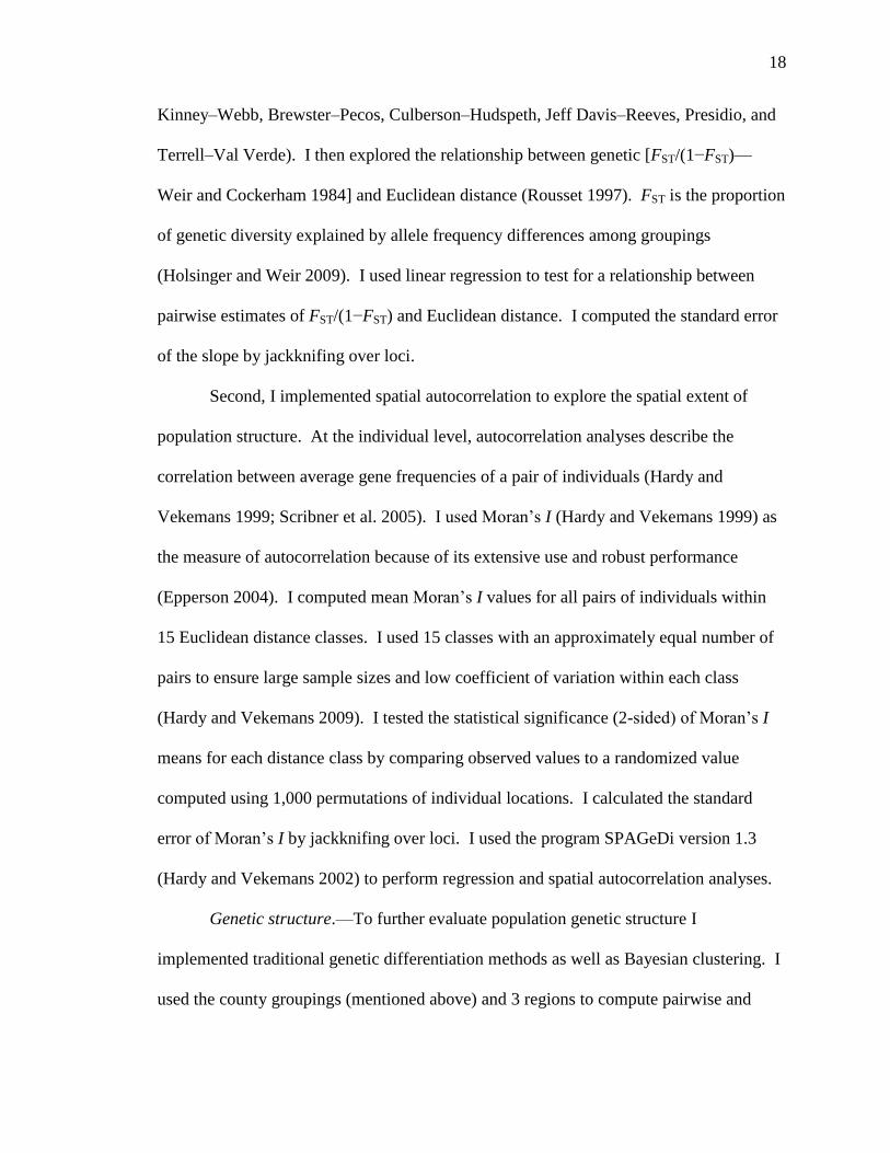
Genetic associations with distance.—I characterized mountain lion genetic

associations with geographic (Euclidean) distance using 2 approaches. First, I grouped

individuals by county, or combined proximate counties (i.e., rough county) to maintain n

≥ 5 (New Mexico—Bernalillo–San Miguel, Dona Ana, Grant–Catron, Hidalgo, and

Socorro–Sierra–Lincoln; Texas—LaSalle–McMullen–Kleberg–Live Oak, Maverick–

18

Kinney–Webb, Brewster–Pecos, Culberson–Hudspeth, Jeff Davis–Reeves, Presidio, and

Terrell–Val Verde). I then explored the relationship between genetic [FST/(1−FST)—

Weir and Cockerham 1984] and Euclidean distance (Rousset 1997). FST is the proportion

of genetic diversity explained by allele frequency differences among groupings

(Holsinger and Weir 2009). I used linear regression to test for a relationship between

pairwise estimates of FST/(1−FST) and Euclidean distance. I computed the standard error

of the slope by jackknifing over loci.

Second, I implemented spatial autocorrelation to explore the spatial extent of

population structure. At the individual level, autocorrelation analyses describe the

correlation between average gene frequencies of a pair of individuals (Hardy and

Vekemans 1999; Scribner et al. 2005). I used Moran’s I (Hardy and Vekemans 1999) as

the measure of autocorrelation because of its extensive use and robust performance

(Epperson 2004). I computed mean Moran’s I values for all pairs of individuals within

15 Euclidean distance classes. I used 15 classes with an approximately equal number of

pairs to ensure large sample sizes and low coefficient of variation within each class

(Hardy and Vekemans 2009). I tested the statistical significance (2-sided) of Moran’s I

means for each distance class by comparing observed values to a randomized value

computed using 1,000 permutations of individual locations. I calculated the standard

error of Moran’s I by jackknifing over loci. I used the program SPAGeDi version 1.3

(Hardy and Vekemans 2002) to perform regression and spatial autocorrelation analyses.

Genetic structure.—To further evaluate population genetic structure I

implemented traditional genetic differentiation methods as well as Bayesian clustering. I

used the county groupings (mentioned above) and 3 regions to compute pairwise and

19

overall FST (Weir and Cockerham 1984) using the computer program ARLEQUIN

version 3.5 (Excoffier and Lischer 2010). I tested statistical significance (2-sided) by

comparing the observed value to a null value derived from 1,023 permutations of

genotypes among groups (i.e., counties or regions).

Next, I applied 2 Bayesian clustering algorithms that incorporate spatial locations.

I employed the algorithm implemented in GENELAND (Guillot et al. 2005a, 2005b)

version 3.2.4 using program R version 2.11.1 (R Development Core Team 2011). This

model uses a Markov chain Monte Carlo (MCMC) approach to infer genetic

discontinuities among geo-referenced genotypes. I evaluated 1–8 possible genetic

clusters (K) with 8 independent runs for each K. I implemented the spatial model with 10

km of uncertainty to account for inexact sample coordinates. I assumed allele

frequencies to be correlated and used 100,000 MCMC iterations while recording 1,000

(thinning = 100). I selected K using the mode of the maximized posterior probability.

Additionally, I applied the Bayesian algorithm described by Corander et al. (2003) using

BAPS version 5. This approach uses stochastic optimization to infer the posterior mode

of genetic structure in the data. I implemented the spatial clustering of individuals

(Corander et al. 2008) and explored K = 1–8 with 8 independent runs. I selected K based

on the partitioning of individuals that maximized the log marginal likelihood. The

optimal partition of individuals in GENELAND and BAPS should minimize Hardy-

Weinberg and linkage disequilibrium within clusters.

Lastly, I employed a nonspatial Bayesian clustering algorithm using the computer

program STRUCTURE version 2.2. This model uses a MCMC to infer genetic clusters

and assign individuals to ancestral populations while minimizing Hardy-Weinberg and

20

linkage disequilibrium within clusters (Prichard et al. 2000). The algorithm also

estimates ancestry proportions (q-values) to each genetic cluster for each individual. I

selected the admixture model and assumed allele frequencies were correlated (Faulsh et

al. 2003). I performed 100,000 MCMC burn-in repetitions to reduce initial configuration

effects, followed by 500,000 MCMC repetitions of data collection. I explored 1–8

genetic clusters, with 8 independent runs to evaluate consistency. I calculated the

arithmetic mean and standard deviation of the log probability of the data [Ln P(D)] across

runs for each K to identify the plateau and determine the optimal number of clusters

(Prichard et al. 2007). I also calculated the ΔK statistic (Evanno et al. 2005) and used q-

values as an index (Prichard et al. 2007) to inform the selection of K.

Assigning origin to dispersers.—I determined origin for dispersers among known

populations and for potential migrants sampled outside of known populations using

Bayesian clustering and assignment tests. I used mean q-values (over 8 runs) from the

STRUCTURE analyses mentioned above and geographic locations to identify long-

distance dispersal among known populations. I defined long-distance as movement from

western Texas to southern Texas or vice versa, and southern Texas to New Mexico or

vice versa (i.e., ≥ 200 km). Similar to previous studies (e.g., Latch et al. 2006, 2008), I

considered individuals residents of a cluster if q > 0.75 and admixed if q was 0.25–0.75.

Next, I used 3 Bayesian assignment methods to assign origin to the potential

dispersers sampled east of known populations. Here, I used assignment methods because

I had determined which known populations exhibited genetic differentiation, and I could

use that information to define reference populations. In other words, assignment methods

are a more explicit way to discern genetic origins when reference populations are known

21

a priori. In all analyses I considered the 3 regions mentioned previously as reference

populations, and the potential dispersers as unknowns. First, I used the modified

assignment approach of Rannala and Mountain (1997) in GeneClass version 2 (Piry et al.

2004). This approach provides likelihood ratio scores for each unknown individual to

each reference population (Piry et al. 2004), and I used scores > 85% to indicate

assignment. Second, I employed the assignment methods implemented in STRUCTURE

version 2.2 (Falush et al. 2003) and BAPS version 5 (Corander et al. 2003). For both

analyses I assumed that K = 3, corresponding to the regional reference populations. I

employed the USEPOPINFO option in STRUCTURE (Faulsh et al. 2003), and executed

100,000 MCMC burn-in and 500,000 data collecting repetitions. I assumed allele

frequencies were correlated, no admixture, and updated frequencies with only reference

individuals. Because results of this analysis can be sensitive to the a priori assigned

migration rate (MIGPRIOR), I analyzed the data using a range of values (i.e., 0.001–

0.10) as suggested by Prichard et al. (2007). The choice of MIGPRIOR did not

substantially influence results, thus I only present results using MIGPRIOR = 0.05

(default value). Because I incorporated prior population information (i.e.,

USEPOPINFO) and assumed no admixture more certainty is associated with assignments

compared to the admixture analysis mentioned above. Thus, I used a more stringent q-

value (q > 0.85) to indicate genetic assignment (Frantz et al. 2006). Finally, I employed

the trained clustering methodology (Corander et al. 2006, 2008b) in BAPS (Corander et

al. 2003). I explored the assignment of each unknown individual to regional reference

populations, one-by-one. To evaluate the strength of assignment to each cluster I

multiplied by 2 the absolute value of change in the log marginal likelihood (i.e., Bayes

22

factor—Corander et al. 2009) of individual i being assigned to the alternative cluster j.

Values of 0 indicate the assigned reference population, and movement to another

population with a change ≥ 6 suggests substantial support for assignment (Kass and

Raftery 1995). A change ≤ 2 indicates poor assignment support.

RESULTS

Genetic data.—I successfully genotyped 245 mountain lions (57% males, 39%

females, and 4% had no sex information) at 11 microsatellite loci (Fig. 2.1). Of the total,

237 genotypes were sampled from known populations in Texas and New Mexico, and 8

were from presumed long-distance dispersers; 1 each from Kerr, Fisher, Deaf Smith,

Edwards, Kimble, Sutton, and Real County, Texas, and Bossier City, Louisiana. Positive

and negative PCR controls were consistent and did not exhibit any contamination. My

genotyping error rate was < 1%.

Estimates of mean heterozygosity, number of alleles/locus, and allelic richness

were moderate for New Mexico and western Texas as well as the total sample (Table

2.1). However, estimates of genetic diversity for southern Texas were 10%–25% lower

than western Texas and New Mexico. Hardy-Weinberg equilibrium tests using FIS

indicated that western Texas, southern Texas, and the total sample did not significantly

deviate from expectations (Table 2.1). New Mexico, however, exhibited a statistically

significant excess of homozygotes.

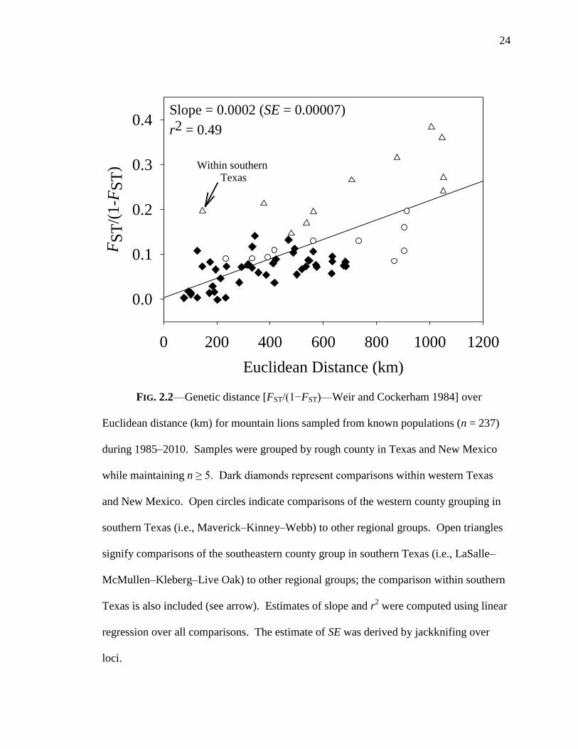
Genetic associations with distance.—I observed a positive linear relationship

(slope = 0.0002, SE = 0.00007) between genetic and Euclidean distance (Fig. 2.2), which

23

TABLE 2.1.—Mean estimates (over 11 loci) of observed (HO) and expected heterozygosity (HE—Nei 1987), number of

alleles/locus (A), allelic richness (ar—Kalinowski 2005) and Hardy-Weinberg equilibrium departure (FIS—Weir and Cockerham

1984) for known mountain lion populations in Texas and New Mexico sampled during 1985–2010. Standard deviations (SD) are in

parentheses, and n indicates sample size.

Region n HO HE A ar FIS

New Mexico 31 0.57 (0.21) 0.61 (0.22) 4.55 (1.64) 4.43 (1.59) 0.07*

Western Texas 178 0.56 (0.22) 0.58 (0.23) 5.09 (1.81) 4.23 (1.39) 0.02

Southern Texas 28 0.45 (0.25) 0.47 (0.25) 3.91 (1.64) 3.85 (1.60) 0.02

Total 237 0.55 (0.21) 0.59 (0.23) 5.55 (1.92) 5.53 (1.90) 0.02

*Significantly different (P < 0.05) than null value derived from 1,023 permutations of alleles among individuals.

24

Euclidean Distance (km)

0 200 400 600 800 1000 1200

FS

T/(

1-F

ST

)

0.0

0.1

0.2

0.3

0.4Slope = 0.0002 (SE = 0.00007)

r2 = 0.49

Within southern Texas

FIG. 2.2—Genetic distance [FST/(1−FST)—Weir and Cockerham 1984] over

Euclidean distance (km) for mountain lions sampled from known populations (n = 237)

during 1985–2010. Samples were grouped by rough county in Texas and New Mexico

while maintaining n ≥ 5. Dark diamonds represent comparisons within western Texas

and New Mexico. Open circles indicate comparisons of the western county grouping in

southern Texas (i.e., Maverick–Kinney–Webb) to other regional groups. Open triangles

signify comparisons of the southeastern county group in southern Texas (i.e., LaSalle–

McMullen–Kleberg–Live Oak) to other regional groups; the comparison within southern

Texas is also included (see arrow). Estimates of slope and r2 were computed using linear

regression over all comparisons. The estimate of SE was derived by jackknifing over

loci.

25

indicated a significant pattern of isolation-by-distance (IBD). Euclidian distance

accounted for approximately half of the variation in genetic distance (r2 = 0.49). Within

the southern Texas region, most pairwise comparisons involving the western counties

(Maverick–Kinney–Webb) followed the predicted IBD pattern. However, all

comparisons including the eastern counties (LaSalle–McMullen–Kleberg–Live Oak)

were greater than the predicted relationship. This indicated that the observed IBD cline

was a poor predictor of genetic distance for the eastern county grouping in southern

Texas.

Spatial autocorrelation analyses (Fig. 2.3) indicated a positive statistical

difference between observed and permuted values for the first 9 distance classes (~20–

250 km), except class 5 (~105 km). Moran’s I values in the first (~20 km) and second

(~40 km) distance class were 2 times greater and equal to second-cousins expectations,

respectively. These higher values indicated high levels of genetic association among

proximate individuals. I observed negative autocorrelation between distance classes 10–

15 (~370–820 km), substantiating the presence of an IBD pattern. Together, linear

regression and spatial autocorrelation provided evidence for an IBD cline, regional level

genetic structure, and genetic association among individuals at distances < 50 km.

Genetic structure.—I observed significant (P < 0.05) overall genetic

differentiation among county groupings (FST = 0.067) and the 3 regions (FST = 0.080)

indicating moderate levels of genetic structure. The regional division appeared to be

more appropriate given FST was higher, accounting for more genetic variation than the

county groupings. Fifty-six of 66 pairwise comparisons among samples grouped by

county were statistically > 0.0 (Table 2.2). Estimates of FST between Texas and New

26

Mean Distance Class (km)

0 200 400 600 800

Mora

n's

I (

SE

)

-0.08

-0.06

-0.04

-0.02

0.00

0.02

0.04

0.06

0.08

0.10

Observed

Permuted

FIG. 2.3—Mean autocorrelation coefficients (Moran’s I—Hardy and Vekemans

1999) and Euclidean distance (km) among all pairs of individuals using 15 distance

classes for known mountain lion populations (n = 237) in Texas and New Mexico

sampled during 1985–2010. Dark circles represent observed Moran’s I values, and light

circles represent null values based on 1,023 permutations of individual locations. Error

bars indicate ± 1 SE, and were computed by jackknifing over loci.

27

TABLE 2.2.—Pairwise estimates of FST (Weir and Cockerham 1984) for mountain lions in Texas and New Mexico sampled

during 1985–2010. Samples were grouped by county or proximate counties to maintain n ≥ 5. Black circles and NS represent

statistically significant (P < 0.05) and not significant estimates, respectively, based on 1,023 permutations of genotypes among groups.

New Mexico

Texas

County groupings

(sample size)

Bernalillo–

San

Miguel

Dona

Ana

Grant–

Catron Hidalgo

Socorro–

Sierra–

Lincoln

LaSalle–

McMullen–

Kleberg–

Live Oak

Maverick–

Kinney–

Webb

Brewster–

Pecos

Culberson–

Hudspeth

Jeff

Davis–

Reeves

Presidio

Terrell–

Val

Verde

Bernalillo–San Miguel

(n = 5) – 0.040 0.074 0.031 0.088

0.267 0.147 0.079 0.077 0.080 0.060 0.068

Dona Ana (n = 5) NS – 0.053 0.014 0.016

0.247 0.117 0.080 0.082 0.074 0.057 0.059

Grant–

Catron (n = 5) NS NS – 0.023 0.064

0.200 0.097 0.072 0.128 0.096 0.074 0.075

Hidalgo (n = 7) NS NS NS – 0.065

0.217 0.133 0.074 0.056 0.102 0.066 0.079

Socorro–

Sierra–Lincoln (n = 9) ● NS ● ● –

0.279 0.069 0.098 0.102 0.118 0.083 0.088

LaSalle–

McMullen–

Kleberg–

Live Oak (n = 21)

● ● ● ● ●

– 0.159 0.124 0.212 0.158 0.144 0.173

Maverick–

Kinney–

Webb (n = 7)

● ● ● ● ●

● – 0.078 0.103 0.089 0.083 0.077

Brewster–

Pecos (n = 30) ● ● ● ● ●

● ● – 0.070 0.016 0.002 0.004

Culberson–

Hudspeth (n = 11) ● ● ● ● ●

● ● ● – 0.069 0.049 0.067

Jeff Davis–

Reeves (n = 52) ● ● ● ● ●

● ● ● ● – 0.011 0.015

Presidio (n = 71) ● ● ● ● ●

● ● NS ● ● – 0.000

Terrell–

Val Verde (n = 14) ● ● ● ● ●

● ● NS ● ● NS –

28

Mexico were moderate–high (0.056–0.279), generally increasing with Euclidean distance

as expected under IBD. All estimates including the LaSalle–McMullen–Kleberg–Live

Oak group were notably high (FST = 0.124–0.279). The 3 pairwise comparisons among

regions were statistically positive (P < 0.05), and further indicated considerable

differentiation associated with southern Texas (New Mexico–southern Texas FST = 0.15,

western Texas–southern Texas FST = 0.10, and New Mexico–western Texas FST = 0.06).

Of the 8 runs using GENELAND, the maximized posterior probability of K

occurred at 3 for 6 runs, and at 5 for 2 runs. However, the maximized probability for all

6 runs at K = 3 was higher than at K = 5. Therefore, I inferred the optimal number of

clusters to be 3 (Fig. 2.4). The clusters of individuals and membership probability

suggested by GENELAND corresponded exactly to the 3 regions; New Mexico, western

Texas, and southern Texas. Similarly, BAPS results indicated that the log marginal

likelihoods for the 10 best visited partitions were maximized at K = 3, providing a

posterior probability of 1 for K = 3. The clustering of individuals from BAPS (Fig. 2.5)

approximately corresponded to New Mexico, western Texas, and southern Texas

corroborating the results from GENELAND.

The STRUCTURE results are less clear than those from GENELAND and BAPS.

The mean Ln P(D) appeared to reach a plateau at K = 2 or 3, peaked at K = 4, and

declined and became more variable at K > 4 (Fig. 2.6). The ΔK statistic of Evanno et al.

(2005) provided moderate support for K = 2 and 3, but high support for K = 4 (Fig. 2.6).

Ancestry proportions (q-values) for most individuals at K = 2, 3, and 4 maintained high

29

FIG. 2.4—Genetic clustering results from GENELAND for known mountain lion populations (n = 237) in Texas and New

Mexico sampled during 1985–2010. A) Map of the estimated genetic membership, which corresponds to the 3 regional groups; New

Mexico, western Texas, and southern Texas. B) Probability surface indicating which samples belong to New Mexico, C) western

Texas, and D) southern Texas. Dark–light colors indicate low–high probabilities of membership.

30

FIG. 2.5—Genetic clustering results from BAPS for known mountain lion

populations (n = 237) in Texas and New Mexico sampled during 1985–2010. A) Colored

Voronoi tessellations around each sample location for all individuals. Colors correspond

to each genetic cluster (K = 3). B) Individual assignments to each genetic cluster with

geographic sampling locations labeled below; New Mexico, southern Texas, and western

Texas. Each column represents 1 individual.

31

A

K

0 1 2 3 4 5 6 7 8 9

Ln

P(D

)

-6600

-6400

-6200

-6000

-5800

-5600

K

1 2 3 4 5 6 7 8

K

0

10

20

30

40

50

60B

FIG. 2.6—The log probability of the data [Ln P(D)] and ΔK (Evanno et al. 2005)

from STRUCTURE for known mountain lion populations (n = 237) in Texas and New

Mexico sampled during 1985–2010. A) Mean Ln P(D) over K for 8 independent runs.

Error bars indicate ± 1 SD, and K is the assumed number of genetic clusters. B) Estimate

of ΔK for K = 2–7 using estimates of Ln P(D) from STRUCTURE.

32

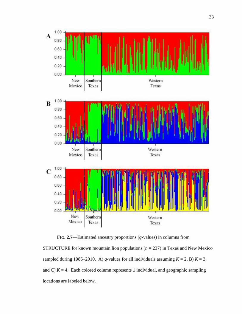
values indicating support for all 3 scenarios (Fig. 2.7). However, at K = 2–4 western

Texas displayed more admixture (q = 25–75%) than the other regions: K = 2—New

Mexico (29%), southern Texas (18%), western Texas (34%); K = 3—New Mexico

(32%), southern Texas (21%), western Texas (66%); K = 4—New Mexico (23%),

southern Texas (18%), western Texas (51%). To examine if there was a biological

feature or association responsible for the additional cluster in western Texas I mapped

individuals assuming K = 4. I included individuals in a cluster only if q was > 0.65.

There was no clear biological interpretation of the additional cluster in western Texas.

Incoherent clustering has been documented in clumped and opportunistic sampling

designs (McRae et al. 2005; Schwartz and McKelvey 2009), as well as in data exhibiting

IBD (Frantz et al. 2009); both of which are characteristic of my data. However, I

conducted exploratory analyses by separating males and females to determine if dispersal

differences were responsible for the additional cluster in western Texas. For both males

(n = 98) and females (n = 73) results indicated K = 1, but when combined Ln P(D) and

ΔK (Evanno et al. 2005) suggested K = 2. Accordingly, I explored genetic differentiation

between sexes in western Texas, which proved to be low (FST = 0.005, P > 0.05). I was

unable to identify biological support for the additional cluster in western Texas.

Therefore, I concluded that my sample was composed of only 3 genetic clusters, a

solution unequivocally supported by FST analyses and 2 of 3 clustering algorithms. The

partition of individuals from GENELAND, BAPS, and STRUCTURE suggested the

clusters generally corresponded to the 3 regions of New Mexico, western Texas, and

southern Texas.

33

FIG. 2.7—Estimated ancestry proportions (q-values) in columns from

STRUCTURE for known mountain lion populations (n = 237) in Texas and New Mexico

sampled during 1985–2010. A) q-values for all individuals assuming K = 2, B) K = 3,

and C) K = 4. Each colored column represents 1 individual, and geographic sampling

locations are labeled below.

34

Assigning origin to dispersers.—I identified long-distance movements among

known populations using mean q-values from STRUCTURE and assuming K = 3. Two

adult males sampled in Jeff Davis and Brewster county, western Texas, exhibited

ancestry to southern Texas (PC040—q = 0.793, SD = 0.010; MLA19—q = 0.933, SD =

0.003). In addition, 2 males and 1 adult female sampled in Maverick, LaSalle, and

Kinney county, southern Texas, exhibited ancestry to New Mexico (PC007—q = 0.780,

SD = 0.005; PC189—q = 0.794, SD = 0.005; and PC121—q = 0.753, SD = 0.008).

Before implementing assignment tests it is important to ensure that a sufficient

number of loci and individuals have been sampled from reference populations (Manel et

al. 2002). Reasonable levels of genetic diversity and differentiation are also required.

My reference populations were composed of 28–178 individuals genotyped at 11 loci

with reasonable levels of HE and FST, which provided adequate power to assign origins

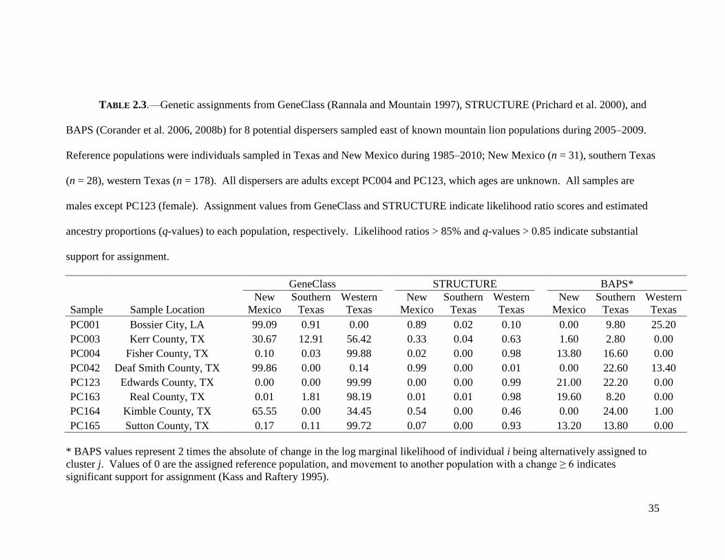
(Latch et al. 2006; Manel et al. 2002). Results from GeneClass, STRUCTURE, and

BAPS were consistent and implied strong genetic assignments for 6 of the 8 potential

dispersers (Table 2.3). PC001 and PC042 were strongly assigned to New Mexico. This

is particularly interesting because PC001 was a male sampled in Bossier City, Louisiana,

> 800 km from New Mexico. The assignment for PC0042 is not surprising because this

male was sampled < 10 km from New Mexico. PC004, PC123, PC163, and PC165 all

exhibited strong assignments to western Texas. These assignments are reasonable

because PC004 was a male sampled in north-central Texas, and PC123 (male), PC163

(female), and PC165 (male) were all sampled in central Texas.

Unfortunately, I was unable to assign 2 dispersers. PC003 was moderately–

weakly assigned to all reference populations by GeneClass and STRUCTURE suggesting

35

TABLE 2.3.—Genetic assignments from GeneClass (Rannala and Mountain 1997), STRUCTURE (Prichard et al. 2000), and

BAPS (Corander et al. 2006, 2008b) for 8 potential dispersers sampled east of known mountain lion populations during 2005–2009.

Reference populations were individuals sampled in Texas and New Mexico during 1985–2010; New Mexico (n = 31), southern Texas

(n = 28), western Texas (n = 178). All dispersers are adults except PC004 and PC123, which ages are unknown. All samples are

males except PC123 (female). Assignment values from GeneClass and STRUCTURE indicate likelihood ratio scores and estimated

ancestry proportions (q-values) to each population, respectively. Likelihood ratios > 85% and q-values > 0.85 indicate substantial

support for assignment.

GeneClass STRUCTURE BAPS*

Sample Sample Location

New

Mexico

Southern

Texas

Western

Texas

New

Mexico

Southern

Texas

Western

Texas

New

Mexico

Southern

Texas

Western

Texas

PC001 Bossier City, LA

99.09 0.91 0.00

0.89 0.02 0.10

0.00 9.80 25.20

PC003 Kerr County, TX

30.67 12.91 56.42

0.33 0.04 0.63

1.60 2.80 0.00

PC004 Fisher County, TX

0.10 0.03 99.88

0.02 0.00 0.98

13.80 16.60 0.00

PC042 Deaf Smith County, TX

99.86 0.00 0.14

0.99 0.00 0.01

0.00 22.60 13.40

PC123 Edwards County, TX

0.00 0.00 99.99

0.00 0.00 0.99

21.00 22.20 0.00

PC163 Real County, TX

0.01 1.81 98.19

0.01 0.01 0.98

19.60 8.20 0.00

PC164 Kimble County, TX

65.55 0.00 34.45

0.54 0.00 0.46

0.00 24.00 1.00

PC165 Sutton County, TX 0.17 0.11 99.72 0.07 0.00 0.93 13.20 13.80 0.00

* BAPS values represent 2 times the absolute of change in the log marginal likelihood of individual i being alternatively assigned to

cluster j. Values of 0 are the assigned reference population, and movement to another population with a change ≥ 6 indicates

significant support for assignment (Kass and Raftery 1995).

36

admixed ancestry. However, BAPS provided essentially no support to any reference

population (i.e., a change < 3 in 2 times the log marginal likelihood) indicating that

PC003 could be from an unsampled source. Further, by all methodologies PC164 was

moderately and weakly assigned to western Texas and New Mexico with essentially no

support for southern Texas. PC164 appeared to be a product of combined ancestry from

New Mexico and western Texas. Overall, assignments from GeneClass, STRUCTURE,

and BAPS indicated long-distance movements have occurred across my sampling area.

DISCUSSION

Disparate patterns of genetic structure have been observed in mountain lions,

ranging from continuous (Anderson et al. 2004; Culver et al. 2000; Sinclair et al. 2001)–

highly structured (Ernest et al. 2003). Genetic and geographic distance associations in

my sample indicated that genetic structure was present from the local–regional scale. At

the local scale (< 50 km), autocorrelation analyses suggested that sampled mountain lions

exhibited genetic associations similar to other large carnivores (Fabbri et al. 2007).

However, family members in southern Texas may have been sampled (Harveson 1997),

inflating these associations. Female philopatry (Logan and Sweanor 2001, 2010;

Sweanor et al. 2000), high sampling effort (e.g., hunting, trapping, etc.) at local scales

(Schwartz and McKelvey 2009), or a combination could further contribute to the non-

independence among proximate individuals. At the regional scale, autocorrelation and

regression analyses identified a significant IBD pattern indicating a decrease in gene flow

with increasing geographic distance. This pattern is consistent with other continuous

(Anderson et al. 2004; Sinclair et al. 2001) as well as structured mountain lion

populations (Ernest et al. 2003; McRae et al. 2005).

37

Traditional FST and Bayesian clustering analyses mostly agreed providing a

consensus for 3 differentiated groups at the regional level (New Mexico, western Texas,

and southern Texas. However, the nonspatial algorithm in STRUCTURE rendered

support for 4 genetic clusters (split western Texas into 2 clusters). Discrepant results

from the clustering algorithms may be due to sampling constraints or ecological

processes. Convenient and clumped sampling schemes (McRae et al. 2005; Schwartz and

McKelvey 2009) as well as patterns of IBD (Frantz et al. 2009), have created spurious

genetic discontinuities in clustering analyses. My sampling scheme was necessarily

clumped and opportunistic, and the data exhibited patterns of IBD producing an

amenable environment for spurious clustering. Alternatively, high harvest of mountain

lions can promote immigration from adjacent populations (Cooley et al. 2009). Mountain

lion harvest is unabated in Texas, and as a result my sample from western Texas may

have had a high proportion of immigrants from surrounding unsampled populations (e.g.,

Mexico). Analyses from STRUCTURE indicated higher levels of admixture within

western Texas, which might provide support for the harvest-immigration hypothesis.

Overall, however, the data provided the most support for K = 3, corresponding to the

regions of New Mexico, western Texas, and southern Texas.

The southern Texas region exhibited high levels of genetic differentiation (FST =

0.10–0.15) when compared to the remaining regions, substantiating the findings from

Walker et al. (2000). Within southern Texas, notable differentiation was displayed by the

county grouping of LaSalle–McMullen–Kleberg–Live Oak (FST = 0.12–0.28). In fact,

these levels were essentially identical to highly fragmented or isolated populations in

southwestern California (Ernest et al. 2003). Additionally, all comparisons including the

38

LaSalle–McMullen–Kleberg–Live Oak group in regression analyses fell above the

predicted IBD relationship, indicating factors other than geographic distance are likely

influencing genetic differentiation.

First, other vagile carnivores (e.g., Lynx—Lynx canadensis) have exhibited

higher differentiation in peripheral populations compared to interior populations

(Schwartz et al. 2003). Peripheral populations can suffer from smaller census sizes,

fewer opportunities for gene flow, and are generally more sensitive to distributional shifts

over time (Schwartz et al. 2003). Southern Texas represents the most peripheral

population in the southwestern U.S., and may have experienced 1 or more of these

mechanisms. Second, the urban development and sprawl throughout central Texas and

along the Mexico-U.S. border has presumably restricted mountain lion movements and

gene flow into southern Texas. Connectivity from adjacent populations to southern

Texas may have also been reduced as a result of predator removal during the 19th

and 20th

century (Wade et al. 1984). This is plausible because removal was targeted around

domestic sheep and goats, which were abundant in most habitats linking western Texas

and Mexico to southern Texas (Lehmann 1969). It may be fruitful to sample museum

specimens to determine if historical differentiation between southern and western Texas

are similar to present levels.

The differentiation I documented between western Texas and New Mexico was

moderate and consistent with other carnivores occupying desert habitats (Onorato et al.

2007). A noteworthy exception was the Culberson–Hudspeth county grouping in western

Texas, which was differentiated from other groupings within the region as well as New

Mexico (FST = 0.05–0.13). The patchy landscape across New Mexico and western Texas

39

could be influencing these levels of differentiation. The landscape matrix is generally

composed of moderate–high quality mountain lion habitat, intervened with low quality

habitat (Young 2009) that presumably impedes movements (Sweanor et al. 2000).

Alternatively, the Culberson–Hudspeth area may be a corridor for individuals moving

from southeastern New Mexico into western Texas. I did not sample southeastern New

Mexico, but previous research suggests mountain lions in that region are differentiated

from western Texas (Gilad et al., in press). Lastly, the clumped sampling in my data

could have contributed to the differentiation associated with the Culberson–Hudspeth

group. Additional research is needed to determine if convenience sampling or natural

process are driving differentiation in this area.

Although many mountain lions populations exhibit genetic differentiation, long-

distance dispersal has been documented (Thompson and Jenks 2010; 2005). My analyses

revealed long-distance movements have occurred across my sampling area, and that

dispersal appeared to be male-biased (11 males, 2 females). Among the known

populations, I documented movement into and out of southern Texas. However, the high

levels of differentiation and lower genetic diversity associated with southern Texas

implies immigrants are not surviving to reproduce. Further investigation is warranted to

determine the reproductive success of dispersers.

For 6 of the 8 potential dispersers sampled eastward New Mexico and western

Texas were the assigned origin. The adult male sampled in Louisiana was > 800 km

from its assigned origin in New Mexico, implying extensive movement. However, an

important note is that our New Mexico reference population may represent a genetic pool

greater than the state boundaries (e.g., southern Rocky Mountains). Dispersers sampled

40

in northern and central Texas were mostly assigned to western Texas, which offers some

support to predicted paths of eastward movement (LaRue and Nielsen 2008). Of the 2

remaining dispersers, 1 exhibited mixed ancestry and the other I could not conclusively

assign. My inability to discern an origin for PC003 suggests that I have not sampled all

sources. Mountain lion movement from Mexico into Texas is probably occurring, and

may explain why I was unable to assign PC003 (a male sampled < 200 km from the

Mexico border). Additional samples from different genetic stocks are needed to

determine origin for this individual, as well as other dispersers throughout the U.S.

I have shown that mountain lions in Texas and New Mexico represent 3 genetic

groups at the regional level with differing levels of connectivity and genetic diversity.

Further, populations in New Mexico, western Texas, and perhaps other unsampled

populations are facilitating eastward mountain lion movements. These finding have clear

implications for management and conservation. First, genetic diversity in New Mexico

and western Texas is at seemingly healthy levels compared to other mountain lion

populations (Culver et al. 2000), and will be maintained if effective population size

remains large (Allendorf and Luikart 2007). Management strategies should aim at

maintaining large effective sizes in these regions to perpetuate diversity and healthy

peripheral populations in the U.S. Southern Texas, however, displayed moderate levels

of genetic diversity along with high levels of differentiation; values comparable to

fragmented or isolated populations in California (Ernest et al. 2003). I did document

natural movements into southern Texas, but reproduction may be negated due to high

mortality as suggested by previous work (Harveson 1997). Natural dispersal into

southern Texas is promising because it has potential to increase diversity and reduce

41

differentiation if reproduction occurs. Strategies should be implemented to increase

fitness of these emigrants during movement and after establishment. For instance,

lowering harvest pressure in potential movement corridors into southern Texas could be 1

alternative. Furthermore, additional research on mountain lions in southern Texas is

needed. It is essential to characterize population productivity and survival because it will

inform the current status and future persistence of mountain lions in this region.

Second, my data suggests that mountain lions in the southwestern U.S. are not

contiguous (Logan and Sweanor 2001; Sweanor et al. 2000). The levels of differentiation

I documented between southern and western Texas is high, and similar to previous work

despite my larger sample size and sampling area. Therefore, I echo the suggestion by

Walker et al. (2000) that western and southern Texas be treated as 2 management units.

This information informs the status of mountain lion connectivity in Texas, and should be

considered when implementing management prescriptions that impact fitness. In

addition, my data indicates New Mexico and western Texas should be considered

separate units connected through moderate levels of genetic exchange. Habitat

conservation for mountain lions in New Mexico, Texas, as well as Mexico will likely

sustain large effective population sizes (Allendorf and Luikart 2007) with high

probabilities of persistence.

Finally, mountain lions from New Mexico and western Texas are moving east.

Mountain lions in New Mexico and Texas will be important to conserve if future

recolonization in the southern U.S. is desired. Additionally, as landscapes continue to

change more research is needed predicting mountain lion movement paths out of known

populations (Sweanor et al. 2000). These efforts would help prioritize important

42

movement corridors and identify locations of high mountain lion-human conflict; both of

which are imperative for the future of mountain lion conservation (Hornocker 2010).

ACKNOWLEDGMENTS

I extend my sincere thanks to Bill Applegate, Louis Harveson, The Museum of

Southwestern Biology - Division of Genomic Resources, Jimmy Rutledge, Johnny

Arredondo, Froylan Hernandez, Richard Dickerson, Billy Pat Mckinney, Ralph Donaho,

Rick Taylor, and James LaCour for providing tissue samples. I thank Eric Redeker for

valuable assistance with GIS applications. The Houston Safari Club, Quail Unlimited,

South Texas Chapter, and Quail Coalition deserve special thanks for valuable scholarship

funds. Financial support for this research was provided by the Texas Parks and Wildlife

Department.

LITERATURE CITED

ALLENDORF, F. W., AND G. LUIKART. 2007. Conservation and the genetics of populations.

Blackwell Publishing, Oxford, United Kingdom.

ANDERSON, C. R., AND F.G. LINDZEY. 2005. Experimental evaluation of population trend

and harvest composition in a Wyoming cougar population. Wildlife Society

Bulletin 33:179–188.

ANDERSON, C. R., F. G. LINDZEY, AND D. B. MCDONALD. 2004. Genetic structure of

cougar populations across the Wyoming basin: metapopulation or

megapopulation. Journal of Mammalogy 85:1207–1214.

ANDERSON, C. R., F. G. LINDZEY, K. H. KNOPFF, M. G. JALKOTZY, AND M. S. BOYCE.

2010. Cougar management in North America. Pp. 41–54 in Cougar ecology and

43

conservation (M. Hornocker and S. Negri, eds.). University of Chicago Press,

Chicago, Illinois.

BAILEY, R. G. 1980. Description of the ecoregions of the United States. U. S. Department

of Agriculture, Miscellaneous Publication 1391:1–77.

BEIER, P. 2010. A focal species for conservation planning. Pp. 177–189 in Cougar

ecology and conservation (M. Hornocker and S. Negri, eds.). University of

Chicago Press, Chicago, Illinois.

COOLEY, H. S., R. B. WIELGUS, G. M. KOEHLER, H. S. ROBINSON, AND B. T. MALETZKE.

2009. Does hunting regulate cougar populations? A test of the compensatory

mortality hypothesis. Ecology 90:2913–2921.

CORANDER J., J. SIRÉN, AND E. ARJAS. 2008a. Bayesian spatial modeling of genetic

population structure. Computational Statistics 23:111–129.

CORANDER, J., P. MARTTINEN, AND S. MANTYNIEMI. 2006. Bayesian identification of

stock mixtures from molecular marker data. Fishery Bulletin 104:550–558.

CORANDER J., P. MARTTINEN, J. SIREN, AND J. TANG. 2009. BAPS: Bayesian analysis of

population structure. Abo Akademi University, Finland, 1–27.

CORANDER J., P. MARTTINEN, J. SIREN, AND J. TANG. 2008b. Enhanced Bayesian

modelling in BAPS software for learning genetic structures of populations. BMC

Bioinformatics 9:539.

CORANDER J., P. WALDMANN, AND M. J. SILLANPAA. 2003. Bayesian analysis of genetic

differentiation between populations. Genetics 163:367–374.

44

CULVER, M., W. E. JOHNSON, J. PECON-SLATTERY, AND S. J. O’BRIEN. 2000. Genomic

ancestry of the American puma (Puma concolor). Journal of Heredity 91:186–

197.

DEYOUNG, R. W., AND R. L HONEYCUTT. 2005. The molecular toolbox: genetic

techniques in wildlife ecology and management. Journal of Wildlife Management

69:1362–1384.

EPPERSON, B. K. 2004. Multilocus estimation of genetic structure within populations.

Theoretical Population Biology 65:227–237.

ERNEST, H. B., W. M. BOYCE, V. C. BLEICH, B. MAY, S. J. STIVER, AND S. G. TORRES.

2003. Genetic structure of mountain lion (Puma concolor) populations in

California. Conservation Genetics 4:353–366.

EVANNO, G., S. REGNAUT, AND J. GOUDET. 2005. Detecting the number of clusters of

individuals using the software STRUCTURE: a simulation study. Molecular

Ecology 14:2611–2620.

EXCOFFIER, L., AND H. LISCHER. 2010. Arlequin suite ver 3.5: a new series of programs to

perform population genetics analyses under Linux and Windows. Molecular

Ecology Resources 10:564–567.

FABBRI, E., ET AL. 2007. From the Apennines to the Alps: colonization genetics of the

naturally expanding Italian wolf (Canis lupus) population. Molecular Ecology

16:1661–1671.

FALUSH, D., M. STEPHENS, AND J. K. PRICHARD. 2003. Inference of population structure

using multilocus genotype data: linked loci and correlated allele frequencies.

Genetics 164:1567–1587.

45

FRANTZ, A. C., ET AL. 2006. Genetic structure and assignment tests demonstrate illegal

translocation of red deer (Cervus elaphus) into a continuous population.

Molecular Ecology 15:3191–3203.

FRANTZ, A. C., S. CELLINA, A. KRIER, L. SCHLEY, AND T. BURKE. 2009. Using spatial

Bayesian methods to determine the genetic structure of a continuously distributed

population: clusters or isolation by distance? Journal of Applied Ecology 46:493–

505.

GILAD, O., J. E. JANEKA, F. ARMSTRONG, M. E. TEWES, AND R. L. HONEYCUTT. In press.

Mountain lions in the Guadalupe National Park: estimates of occurrence and

distribution through DNA analysis. Southwestern Naturalist.

GUILLOT, G., A. ESTOUP, F. MORTIER, AND J. F. COSSON. 2005a. A spatial statistical

model for landscape genetics. Genetics 170:1261–1280.

GUILLOT, G., F. MORTIER, AND A. ESTOUP. 2005b. Geneland: a computer package for

landscape genetics. Molecular Ecology Notes 5:712–715.

HAAG, T., ET AL. 2010. The effect of habitat fragmentation on the genetic structure of a

top predator: loss of diversity and high differentiation among remnant populations

of Atlantic Forest jaguars (Panthera onca). Molecular Ecology 19:4906–4921.

HARDY, O. J., AND X. VEKEMANS, 1999. Isolation by distance in a continuous population:

reconciliation between spatial autocorrelation analysis and population genetics

models. Heredity 83:145–154.

HARDY O. J., AND X. VEKEMANS. 2002. Spagedi: a versatile computer program to analyze

spatial genetic structure at the individual or population levels. Molecular Ecology

Notes 2:618–620.

46

HARDY O. J., AND X. VEKEMANS. 2009. SPAGeDi 1.3 a program for spatial pattern

analysis of genetic diversity. Universite Libre de Bruxelles, Brussels, Belgium, 1–

33.

HARVESON, L. A. 1997. Ecology of a mountain lion population in southern Texas. Ph.D.

dissertation, Texas A&M University & Texas A&M University-Kingsville,

College Station, Texas.

HARVESON, L. A., M. E. TEWES, N. J. SILVY, AND J. RUTLEDGE. 1996. Mountain lion

research in Texas: past, present, and future. Pp. 45–54 in Proceedings of the fifth

mountain lion workshop (W. D. Padly, ed.). Department of Fish and Game, San

Diego, California.

HOLSINGER, K. E., AND B. S. WEIR. 2009. Genetics in geographically structured

populations: defining, estimating and interpreting FST. Nature Reviews Genetics

10:639–650.

HORNOCKER, M. 2010. Pressing buisness. Pp. 235–247 in Cougar ecology and

conservation (M. Hornocker and S. Negri, eds.). University of Chicago Press,

Chicago, Illinois.

KALINOWSKI, S. T. 2005. HP-RARE 1.0: a computer program for performing rarefaction

on measures of allelic richness. Molecular Ecology Notes 5:187–189.

KASS, R. E., AND A. E. RAFTERY. 1995. Bayes factors. Journal of the American Statistical

Association 90:773–795.

LARUE, M. A., AND C. K. NIELSEN. 2008. Modelling potential dispersal corridors for

cougars in midwestern North America using least-cost path methods. Ecological

Modelling 212:372–381.

47

LATCH, E. K., G. DHARMARAJAN, J. C. GLAUBITZ, AND O. E. RHODES. 2006. Relative

performance of Bayesian clustering software for inferring population substructure

and individual assignment at low levels of population differentiation.

Conservation Genetics 7:295–302.

LATCH, E. K., D. G. SCOGNAMILLO, J. A. FIKE, M. J. CHAMBERLAIN, AND O. E. RHODES.

2008. Deciphering ecological barriers to North American river otter (Lontra

canadensis) gene flow in the Louisiana landscape. Journal of Heredity 99:265–

274.

LEHMANN, V. W. 1969. Forgotten legions. Texas Western Press, University of Texas-El

Paso, El Paso, Texas.

LOGAN, K. A., AND L. L. SWEANOR. 2001. Desert puma: evolutionary ecology and

conservation of an enduring carnivore. Island Press, Washington D.C., United

States.

LOGAN, K. A., AND L. L. SWEANOR. 2010. Behavior and social organization of a solitary

carnivore. Pp. 105–117 in Cougar ecology and conservation (M. Hornocker and

S. Negri, eds.). University of Chicago Press, Chicago, Illinois.

LONGMIRE, J. L., M. MALTBIE, AND R. J. BAKER. 1997. Use of lysis buffer in DNA

isolation and its implications for museum collections. Occasional Papers,

Museum of Texas Tech University 163:1–3.

MANEL, S., P. BERTHIER, AND G. LUIKART. 2002. Detecting wildlife poaching: identifying

the origin of individuals with Bayesian assignment tests and multilocus

genotypes. Conservation Biology 16:650–659.

48

MCRAE, B. H., P. BEIER, L. E. DEWALD, L. Y. HUYNH, AND P. KEIM. 2005. Habitat

barriers limit gene flow and illuminate historical events in a wide-ranging

carnivore, the American puma. Molecular Ecology 14:1965–1977.

MENOTTI-RAYMOND, M., ET AL. 1999. A genetic linkage map of microsatellites in the

domestic cat (Felis catus). Genomics 57:9–23.

NEI, M. 1987. Molecular evolutionary genetics. Columbia University Press, New York,

New York.

ONORATO, D. P., E. C. HELLGREN, R. A. VAN DEN BUSSCHE, D. L. DOAN-CRIDER, AND J.

R. SKILES. 2007. Genetic structure of American black bears in the desert

southwest of North America: conservation implications for recolonization.

Conservation Genetics 8:565–576.

PIERCE, B. M., AND V. C. BLEICH. 2003. Mountain lion (Puma concolor). Pp. 744–757 in

Wild mammals of North America: biology, management, and conservation. (G.

A. Feldhammer, B. C. Thompson, and J. A. Chapman, eds.). 2nd

ed. The John

Hopkins University Press, Baltimore, Maryland.

PIRY, S., A. ALAPETITE, J. M. CORNUET, D. PAETKAU, L. BAUDOUIN, AND A. ESTOUP.

2004. GeneClass2: a software for genetic assignment and first-generation migrant

detection. Journal of Heredity 95:536–539.

PITTMAN, M. T., G. J. GUZMAN, AND B. P. MCKINNEY. 2000. Ecology of the mountain

lion on Big Bend Ranch State Park in Trans-Pecos region of Texas. Texas Parks

and Wildlife Department, Final Report Project Number 86, Austin, Texas.

PRITCHARD, J. K., M. STEPHENS, AND P. DONNELLY. 2000. Inference of population

structure using multilocus genotype data. Genetics 155:945–959.

49

PRITCHARD, J. K., X. WEN, AND D. FAULSH. 2007. Documentation for structure software:

version 2.2. University of Chicago, Chicago, Illinois, 1–36.

RANNALA, R., AND J. L. MOUNTAIN. 1997. Detecting immigration by using mulilocus

genotypes. Proceedings of the National Academy of Sciences USA 94:9197–

9201.

R DEVELOPMENT CORE TEAM. 2011. R: a language and environment for statistical

computing. R Foundation for Statistical Computing, Vienna, Austria.

http://www.R-project.org. Accessed 14 March 2011.

ROUSSET, F. 1997. Genetic differentiation and estimation of gene flow from F-statistics

under isolation by distance. Genetics 145:1219–1228.

RUSS, W. B. 1996. The status of the mountain lion in Texas. Pp. 30–31 in Proceedings of

the fifth mountain lion workshop (W. D. Padly, ed.). Department of Fish and

Game, San Diego, California.

SCHMIDLY, D. J. 2004. The mammals of Texas. 6th ed. University of Texas Press, Austin,

Texas.

SCHWARTZ, M. K., AND K. S. MCKELVEY. 2009. Why sampling scheme matters: the

effect of sampling scheme on landscape genetic results. Conservation Genetics

10:411–452.

SCHWARTZ, M. K., L. S. MILLS, Y. ORTEGA, L. F. RUGGIERO, AND F. W. ALLENDORF.

2003. Landscape location affects genetic variation of Canada lynx (Lynx

canadensis). Molecular Ecology 12:1807–1816.

50

SCRIBNER, K. T., ET AL. 2005. Geographical genetics: conceptual foundations and

empirical applications of spatial genetic data in wildlife management. Journal of

Wildlife Management 69:1434–1453.

SINCLAIR, E. A., E. L. SWENSON, M. L. WOLFE, D. C. CHOATE, B. GATES, AND K. A.

CRANALL. 2001. Gene flow estimates in Utah’s cougars imply management

beyond Utah. Animal Conservation 4:257–264.

SPONG, G., M. JOHANSSON, AND M. BJORKLUND. 2000. High genetic variation in leopards

indicates large and long-term stable effective population size. Molecular Ecology

9:1773–1782.

SWEANOR, L. L., K. A. LOGAN, AND M. G. HORNOCKER. 2000. Cougar dispersal patterns,

metapopulation dynamics, and conservation. Conservation Biology 14:798–808.

THOMPSON, D. J., AND J. A. JENKS. 2010. Dispersal movements of subadult cougars from

the Black Hills: the notions of range expansion and recolonization. Ecosphere

1:1–11.

THOMPSON, D. J., AND J. A. JENKS. 2005. Long-distance dispersal by a subadult male

cougar from the Black Hills, South Dakota. Journal of Wildlife Management

69:818–820.

WADE, D. A., D. W. HAWTHORNE, G. L. NUNLEY, AND M. CAROLINE. 1984. History and

status of predator control in Texas. Pp 122–131 in Proceedings of the Eleventh

Vertebrate Pest Conference (D. O. Clark, ed.). University of Nebraska, Lincoln.

WALKER, C. W., L. A. HARVESON, M. T. PITTMAN, M. E. TEWES, AND R. L. HONEYCUTT.

2000. Microsatellite variation in two populations of mountain lions (Puma

concolor) in Texas. Southwestern Naturalist 45:196–203.

51

WASSER, S. K., ET AL. 2008. Combating the illegal trade in African elephant ivory with

DNA forensics. Conservation Biology 22:1065−1071.

WEIR, B. S., AND C. C. COCKERHAM. 1984. Estimating F-statistics for the analysis of

population structure. Evolution 38:1358–1370.

YOUNG, J. H. 2009. Estimating mountain lion population parameters in Texas. Ph.D.

dissertation, Texas A&M University-Kingsville, Kingsville, Texas.

YOUNG, J. H., M. E. TEWES, A. M. HAINES, G. GUZMAN, AND S. J. DEMASO. 2010.

Survival and mortality of cougars in the Trans-Pecos region. Southwestern

Naturalist 55:411–418.

Chapter 3 of this thesis follows the format of the Journal of Applied Ecology.

52

CHAPTER III

THE DEMOGRAPHIC HISTORY OF AN ELUSIVE CARNIVORE: USING

MUSEUMS TO INFORM MANAGEMENT

Summary

1. Characterizing population trends is a priority for wildlife managers. Unfortunately,

surveying elusive and inconspicuous carnivores is extremely difficult. I applied a

retrospective genetic approach to examine how historical and recent conditions

influenced the demographic history of mountain lions Puma concolor in Texas.

2. I sampled archived and recent genetic material and amplified 10 microsatellite loci. I

indexed population trends by estimating historical and recent genetic diversity, spatial

and temporal genetic differentiation and effective population size.

3. Mountain lions in southern Texas exhibited a 10–20% decline in genetic diversity

over time, whereas all estimates were similar for western Texas. From historical–current

conditions, genetic differentiation between western and southern Texas increased by 2.5

times. Temporal genetic differentiation in southern Texas was 7 times that of western

Texas, which appeared to be responsible the increase in genetic differentiation between

western and southern Texas.

4. Estimates of effective population size revealed a much lower average population size

in southern Texas relative to western Texas. Southern Texas also exhibited a > 50%

decline in effective size over time, whereas estimates for western Texas indicated

population stability.

53

5. Synthesis and applications. All evidence suggests mountain lions in western Texas

have remained at high and relatively stable levels over time. In contrast, my results show

dramatic temporal declines and changes have occurred in southern Texas. Lower genetic

diversity in southern Texas, and high genetic structure between southern and western

Texas is a recent phenomenon. Furthermore, additional research examining population

productivity and survival in southern Texas is essential. Management actions such as

population monitoring and harvest reduction may be needed to ensure the persistence of

mountain lions in this region. This study emphasizes the importance and utility of

genetically sampling museum and recent specimens to assist wildlife management and

conservation.

Key-words: Effective size, genetic differentiation, genetic diversity, microsatellite loci,

museum specimens, population trends, Puma concolor, Texas

Introduction

An important component of natural resource conservation and management is monitoring

population trends (Marsh & Trenham 2007). Changes in census size and demographic

parameters can inform harvest prescriptions, population augmentation, introductions and

overall conservation status (Witmer 2005). However, implementing a monitoring

program using traditional techniques such as marking individuals can be logistically and

financially demanding (Barea-Azcon et al. 2007). This is particularly true for territorial,

inconspicuous and elusive species that inhabit dense or rugged habitats (Witmer 2005);

many large carnivores exemplify these characteristics.

Genetic tools have been employed in many ways to assist the monitoring of

carnivore populations (e.g., De Barbra et al. 2010). Genetic data can discriminate

54

individuals or species and thus provide estimates of abundance, vital rates and

characterize changes in geographic distribution (Schwartz, Luikart & Waples 2006). The

use of genetic data has become relatively common to investigate the abundance and

distribution of many carnivore species (Boulanger, Himmer & Swan 2004; McKelvey et

al. 2006). Furthermore, genetic techniques can be used to assess demographic trends

through time (Wandeler, Hoeck & Keller 2007). Comparison of genetic data from

museum specimens to contemporary samples can elucidate the effects of historical and

recent events on genetic diversity and structure. The genetic analysis of historical

samples has informed the conservation and management of brown bears Ursus arctos

(L.) (Miller & Waits 2003), Florida panthers Puma concolor coryi (B.) (Culver et al.

2008) and gray wolves Canis lupus (L.) (Flagstad et al. 2003).

Throughout North America mountain lions Puma concolor (L.) have experienced

severe declines in census size and geographic distribution because of habitat loss and

predator management policies (Logan & Sweanor 2001; Anderson et al. 2010).

Currently, populations mainly inhabit the western half of the continent. During the mid–

late 1900s most western states in the United States modified policies and regulated the

harvest of mountain lions (Anderson et al. 2010). Regulation allowed populations in

some areas to recover to high levels (Logan & Sweanor 2001). Today, large populations

generally exhibit moderate levels of genetic diversity and low genetic differentiation

(Culver et al. 2000; Anderson, Lindzey & McDonald 2004). Small and peripheral

populations exhibit lower diversity and high differentiation (Walker et al. 2000; Ernest et

al. 2003).

55

In Texas, USA, mountain lions are peripheral to the greater distribution and

breeding populations occur only in the western and southern portions of the state (Fig.

3.1; Schmidly 2004). The harvest of mountain lions is not regulated in Texas and

mandatory inspection is not required (Harveson et al. 1996; Russ 1996; Anderson et al.

2010). Therefore, harvest cannot be used by managers to inform demographic indices of

population trends (e.g., Anderson & Lindzey 2005). Furthermore, little information is

available to assist mountain lion management in Texas. Previous studies indicate all

Texas populations have young age structures (Harveson et al. 1996), and exhibit low

survival (Harveson 1997; Young et al. 2010) and reproduction (Harveson 1997; Pittman,

Guzman & McKinney 2000). Genetic data suggest low diversity in southern Texas and

genetic structure between southern and western Texas, implying southern Texas may be

isolated (Walker et al. 2000). Together, unlimited harvest and sparse information

warrant management concern, and additional research is clearly needed.

My overall goal was to assess the demographic history of mountain lions in Texas

over the past century using microsatellite DNA data. Microsatellite loci are highly

variable genetic markers and consist of tandem repeats of a short sequence motif

(Allendorf & Luikart 2007). I used historical and contemporary samples from western

and southern Texas to estimate (i) genetic diversity, (ii) spatial genetic differentiation,

(iii) temporal genetic differentiation and (iv) effective population size. My genetic

approach also allowed me to determine if high differentiation and low diversity in

southern Texas (Walker et al. 2000) was present historically.

56

Fig. 3.1. Mountain lion sampling distribution throughout western and southern Texas, USA. (a) Samples from western Texas

during 1935–1955 (median = 1938; n = 27) and southern Texas during 1934–1942 (median = 1937; n = 34). (b) Samples from

western Texas during 1979–1989 (median = 1983; n = 42). (c) Samples from western Texas during 2000–2010 (median = 2006; n =

168) and southern Texas during 1985–2009 (median = 1996; n = 28).

57

Materials and methods

I obtained tissue samples from mountain lions collected in western and southern Texas

spanning the temporal period 1905–2010. For the historical samples, I collected c. 100–

200 mg of bone material taken from the maxilloturbinates of mountain lion skulls housed

in museum collections, following Wisely, Maldonado & Fleischer (2004). The

contemporary samples consisted of muscle tissues donated by hunters and trappers,

collected from road-kills, or taken from live-trapped individuals during previous research.

Muscle tissue was frozen, dried or placed in lysis buffer (Longmire, Maltbie & Baker

1997) and stored at -20 °C prior to DNA extraction.

I used separate protocols to extract DNA from muscle tissue and maxilloturbinate

samples. For muscle tissue, I extracted DNA using the DNeasy Tissue Kit and a

commercial protocol (Qiagen). For maxilloturbinates, I ground samples using a mortar

and pestle and placed them in lysis buffer (0∙5 M EDTA pH 8∙0, 0∙5% SDS and 0∙5

mg/ml proteinase K; Wang, Woiderski & Driver 2005). I handled a maximum of nine

samples (eight maxilloturbinate samples and one extraction negative) during each

extraction day to reduce the potential for cross-contamination. I incubated samples for ≥

24 h at 50 °C and extracted DNA using a QIAquick PCR Purification Kit (Qiagen,

California, USA) and a modified extraction protocol developed by Wang et al. (1998) for

ancient DNA samples.

Maxilloturbinates from museum specimens generally exhibit lower DNA quality

and quantity than modern tissue resulting in a higher probability of contamination during

extraction and PCR-setup (Wandeler, Hoeck & Keller 2007). Therefore, I extracted

DNA and prepared PCRs for all maxilloturbinate samples in an isolated laboratory where

58

no mammalian DNA had previously been extracted or amplified. All materials used for

DNA extraction and PCR were designated only for that purpose and were cleaned with

RNAse Away® (Molecular BioProducts, California, USA) or 50% bleach before and

after use.

For each individual I used the polymerase chain reaction (PCR) to amplify 10

microsatellite loci (FCA008, FCA035, FCA043, FCA077, FCA082, FCA090, FCA096,

FCA133, FCA176, FCA205) described by Menotti-Raymond et al. (1999). I amplified

loci individually in 10 µL reaction volumes that contained 5 µL AmpliTaq Gold® PCR

Master Mix (Applied Biosystems), 0∙24 µM of each primer, and 1–1∙5 µL of extracted

DNA. However, for maxilloturbinate reactions I increased primer concentration to 0∙50

µM, added 0∙2 mg/µL of bovine serum albumin, and increased the quantity of extracted

DNA to 1∙5–2∙5 µL. I used a touchdown PCR profile with an initial denaturation at 94

°C for 10 min, 20 cycles of 94 °C for 30 s, 62 °C for 30 s, 61 °C for 30 s, 60 °C for 30 s,

and 72 °C for 60 s, followed by 30 cycles of 94 °C for 30 s, 55 °C for 90 s, and 72 °C for

60 s, with a final extension of 60 °C for 10 min. For maxilloturbinate reactions I reduced

the first set of temperature cycles to 10 and increased the second set to 50. I combined 3

µL of PCR products for each individual and applied 1∙5–2 µL of the PCR product mix to

a denaturing formamide (Hi-Di Formamide; Applied Biosystems) and size standard

mixture (GeneScan ROX 500; Applied Biosystems). I loaded the resulting mixtures onto

a 3130xl genetic analyzer (Applied Biosystems) for fragment separation. I included a

positive and negative PCR control with each run through the analyzer to identify

contamination and run consistency. I inspected all loci and sized alleles using

59

GeneMapper® software v4.0 (Applied Biosystems). I re-ran 10% of muscle tissue

samples used in analyses to calculate a genotyping error rate.

Additional measures are required to ensure genotypes are correct for museum

samples because extracted DNA is at relatively low concentrations and quality

(Wandeler, Hoeck & Keller 2007; Casas-Marce, Revilla & Godoy 2009). Errors can

occur from contamination, allelic dropout and false alleles when using museum

specimens (Miller & Waits 2003; Wandeler, Hoeck & Keller 2007). Therefore, in

addition to the positive and negative PCR controls aforementioned, I attempted to

amplify all extraction negatives several times to detect potential cross-contamination

during DNA extraction. Additionally, I performed 2–5 separate reactions for each

individual at each locus and only called alleles I observed ≥ 2 times.

DATA ANALYSIS

The historical and recent samples represented three temporal periods for western Texas

(1935–1955, 1979–1989 and 2000–2010) and two periods for southern Texas (1934–

1942 and 1985–2009); all temporal samples had n ≥ 27 individuals. The median years

for the western Texas samples were 1938, 1983 and 2006, and the southern Texas

medians were 1937 and 1996 (see Appendix S1 for museum specimens used).

I created input files for data analyses using the computer program CONVERT

(Glaubitz 2004). I tested Hardy-Weinberg expectations (HWE) using FIS (Weir &

Cockerham 1984) for two pooled statewide samples spanning the temporal periods of

1934–1955 and 1985–2010. I also assessed HWE for each temporal sample (i.e.,

southern Texas: 1937, 1996; western Texas: 1938, 1983 and 2006). I evaluated statistical

significance (2-sided) by comparing the observed FIS value against a null value computed

60

from 1023 permutations of alleles among individuals in the computer program ARLEQUIN

3.5 (Excoffier & Lischer 2010).

I performed several analyses to characterize changes in genetic diversity over

time. I estimated observed heterozygosity (HO), expected heterozygosity (HE; Nei 1987),

number of alleles (A) and allelic richness (ar) per locus for each temporal sample. I

calculated HO, HE and A using the computer program ARLEQUIN 3.5 (Excoffier & Lischer

2010) and ar using HP-RARE 1.0 (Kalinowski 2004, 2005). I tested for temporal changes

in ar within southern and western Texas using a Wilcoxon signed rank test (one-sided).

During demographic declines such as population bottlenecks alleles are lost before

heterozygosity changes (Allendorf 1986; Leberg 2002; Schwartz, Luikart & Waples

2006). The estimates of ar use a rarefaction method (Hurlbert 1971; Kalinowski 2004) to

enable comparisons among unequal sample sizes.

Previous research indicated that mountain lions in western and southern Texas

may be genetically differentiated (FST > 0.10), and that HO in southern Texas was 40%

lower than in western Texas (Walker et al. 2000). I estimated FST (Weir & Cockerham

1984) between southern and western Texas for the temporal period of 1934–1955 and

1985–2010 to determine if structure was present historically. FST is the proportion of

genetic diversity explained by allele frequency differences among groups (Holsinger &

Weir 2009). Next, I evaluated the magnitude of genetic change over time within each

geographic region by calculating FST (Weir & Cockerham 1984) among the temporal

samples. This analysis produced one estimate for southern Texas (1937–1996) and three

estimates for western Texas (1938–1983, 1983–2006 and 1938–2006). I calculated FST

using the computer program ARLEQUIN 3.5 (Excoffier & Lischer 2010) and determined

61

statistical significance (2-sided) by comparing the observed value to a null value based on

1023 permutations of genotypes among groups (i.e., regions or temporal periods).

I estimated variance (NeV) and inbreeding (NeI) effective population size for

southern and western Texas to explicitly test for changes in population size over time.

Effective population size is the size of an idealized population exhibiting the same rate of

genetic change as the sampled population (Wright 1931). I used temporal changes in

allele frequencies (Krimbas & Tsakas 1971; Waples 1989) and linkage disequilibrium

(LD) among loci (Hill 1981) to derive estimates of NeV and NeI, respectively. Both

methodologies make simplifying assumptions (e.g., Waples 1989; Leberg 2005; Waples

2006; Luikart et al. 2010) including population closure and no substructure.

The temporal method requires two or more temporally spaced samples of a

species with non-overlapping generations to estimate NeV. When applying temporal

estimators to age structured species such as mountain lions it is important to describe how

samples are pooled over time, define a generation, and identify the number of generations

separating samples (Waples & Yokota 2007). For each discrete temporal sample from

southern and western Texas I used the median year as the pooled year (described

previously). I considered six years as a mountain lion generation because it was the mean

age of adults in a neighboring population exposed to hunting (Logan & Sweanor 2001).

My temporal samples from western and southern Texas covered a range of c. 4–11

mountain lion generations, which should ensure relatively unbiased and precise estimates

of NeV (Waples & Yokota 2007).

I estimated NeV using a moment-based (Krimbas & Tsakas 1971; Nei & Tajima

1981; Pollock 1983; Waples 1989), Bayesian (Berthier et al. 2002) and pseudo-likelihood

62

(Wang 2001) method in the computer program NeEstimator 1.3 (Peel, Overden & Peel

2004) and MLNE 1.0 (Wang & Whitlock 2003). I employed 1000 updates in the Bayesian

framework, and assumed a maximum NeV = 500 for western and southern Texas using the

Bayesian and likelihood methods (Wang 2001; Berthier et al. 2002).

Estimates of NeI do not require temporally spaced samples (Luikart et al. 2010). I

explored temporal changes in NeI using the LD approach of Waples (2006) for each

temporal sample from southern and western Texas. This produced five estimates

separated by 4–11 generations, which should allow me to identify trends in population

size (Tallmon et al. 2010). However, in age-structured samples estimates of NeI based on

the LD method reflect the effective number of breeders (Nb) that produced the cohorts

present in each sample (Waples & Do 2010). Therefore, I used the computer program

LDNE 1.31 (Waples & Do 2008) to compute Nb estimates and calculate 95% CIs

following a jackknifing procedure. I employed the random mating model rather than the

monogamy model because mountain lions exhibit a polygynous mating system (Murphy

1998). To reduce potential bias in the Nb estimates I only used alleles that were present at

frequencies > 0∙02 in analyses (Waples & Do 2010).

Results

I genotyped 10 microsatellite loci for 299 mountain lions (2% missing data) collected

from Texas (50% males, 46% females, and 4% unknown). The sample sizes for the

median year groups from western Texas included n = 27 (1938), n = 42 (1983) and n =

168 (2006), and n = 34 (1937) and n = 28 (1996) from southern Texas (Fig. 3.1). All

positive PCR controls were consistent, and extraction and PCR negatives exhibited no

contamination. My genotyping error rate for muscle tissues was < 1%.

63

GENETIC DIVERSITY AND DIFFERENTIATION

I observed a statistically positive FIS for the recent (1985–2010) statewide sample

indicating HWE were not satisfied (FIS = 0∙04, P = 0∙02). FIS for the historical statewide

sample (1934–1955) was also positive and approached statistical significance suggesting

deviations from HWE (FIS = 0∙05, P = 0∙06). In contrast, both temporal groups from

southern Texas (1937: FIS = 0∙04, P > 0∙05; 1996: FIS = 0∙04, P > 0∙05) and all groups

from western Texas (1938: FIS = 0∙02, P > 0∙05; 1983: FIS = -0∙05, P > 0∙05; 2006: FIS =

0∙00, P > 0∙05) satisfied HWE. Departures from HWE in statewide samples suggested a

Wahlund effect (Allendorf & Luikart 2007).

Estimates of HO, HE and A for each temporal period in western Texas indicated

only minor changes over time (Table 3.1) with mean HE ranging from 0∙59–0∙56 during

1938–2006. I detected no difference in ar (Table 3.2) for any comparisons conducted

within western Texas (1938–1983, 1983–2006 and 1938–2006: Wilcoxon T = -0∙36, P =

0∙36). Levels of diversity in the historical sample from southern Texas are similar to

diversity in western Texas. However, over time I documented a 20% decline in HO and

HE, and a 12% decline in A within southern Texas (Table 3.1). I also observed a

temporal reduction in ar (Table 3.2) that approached statistical significance (1937–1996:

Wilcoxon T = -1∙58, P = 0∙06).

Genetic differentiation between southern and western Texas for the historical

sample was moderate (1934–1955: FST = 0∙04, P < 0∙01), but more than doubled in the

recent sample (1985–2010: FST = 0∙10, P < 0∙01). I observed low yet significant

temporal genetic differentiation within western Texas (1938–1983: FST = 0∙03, P < 0∙01;

1983–2006: FST = 0∙01, P < 0∙01; 1938–2006: FST = 0∙02, P < 0∙01). Southern Texas,

64

Table 3.1. Genetic diversity estimates (HO, HE, A) per locus for geographic and temporal samples (listed by median) of Texas

mountain lions

Western Texas Southern Texas

1938 (n = 27)

1983 (n = 42)

2006 (n = 168)

1937 (n = 34)

1996 (n = 28)

Locus HO HE A HO HE A HO HE A HO HE A HO HE A

FCA008 0∙07 0∙07 3

0∙05 0∙05 2

0.00 0.00 1

0∙09 0∙11 2

0.00 0.00 1

FCA082 0∙70 0∙77 6

0∙75 0∙63 5

0∙52 0∙62 6

0∙47 0∙51 5

0∙58 0∙53 4

FCA090 0∙70 0∙77 6

0∙76 0∙77 6

0∙77 0∙76 7

0∙65 0∙75 7

0∙71 0∙78 6

FCA133 0∙63 0∙51 5

0∙57 0∙55 5

0∙53 0∙55 6

0∙71 0∙57 4

0∙64 0∙61 5

FCA176 0∙44 0∙57 4

0∙33 0∙39 4

0∙41 0∙40 5

0∙43 0∙49 3

0∙11 0∙10 3

FCA035 0∙59 0∙60 3

0∙73 0∙69 4

0∙66 0∙63 6

0∙52 0∙50 4

0∙42 0∙48 3

FCA043 0∙81 0∙80 5

0∙64 0∙67 5

0∙70 0∙75 6

0∙67 0∙75 6

0∙56 0∙58 6

FCA077 0∙48 0∙48 2

0∙55 0∙54 3

0∙54 0∙52 3

0∙41 0∙46 3

0∙14 0∙25 2

FCA096 0∙43 0∙67 4

0∙78 0∙78 5

0∙76 0∙78 5

0∙56 0∙70 5

0∙56 0∙56 5

FCA205 0∙67 0∙65 4 0∙66 0∙61 4 0∙67 0∙63 4 0∙59 0∙68 4 0∙46 0∙52 3

Mean

(SD*)

0∙55

(0∙21)

0∙59

(0∙21)

4∙20

(1∙32)

0∙58

(0∙23)

0∙57

(0∙22)

4∙30

(1∙16)

0∙56

(0∙23)

0∙56

(0∙23)

4∙90

(1∙79)

0∙51

(0∙18)

0∙55

(0∙19)

4∙30

(1∙49)

0∙42

(0∙25)

0∙44

(0∙24)

3∙80

(1∙69)

*Represents the standard deviations of estimate across loci.

65

Table 3.2. Allelic richness estimates per locus for temporal samples (listed by median) of

mountain lions from western and southern Texas

Western Texas

Southern Texas

Locus 1938

(n = 27)

1983

(n = 42)

2006

(n = 168)

1937

(n = 34)

1996

(n = 28)

FCA008 2.56 1.75 1.00

1.98 1.00

FCA082 6.00 4.89 4.51

4.50 3.96

FCA090 5.94 5.49 5.21

6.33 5.94

FCA133 4.56 4.39 4.80

3.62 4.68

FCA176 4.00 3.94 4.14

3.00 2.69

FCA035 3.00 3.94 4.21

3.58 2.99

FCA043 5.00 4.50 4.57

5.94 5.47

FCA077 2.00 2.94 2.55

2.62 2.00

FCA096 4.00 5.00 5.00

4.58 4.89

FCA205 4.00 3.51 3.83

3.95 2.94

Mean 4.11 4.03 3.98

4.01 3.66

SD* 1.34 1.10 1.28

1.38 1.59

*Represents the standard deviations of estimate across loci.

66

however, displayed temporal genetic differentiation seven times greater (1937–1996: FST

= 0∙13, P < 0∙01) than western Texas.

EFFECTIVE POPULATION SIZE

Estimates of NeV using the temporal approach produced statistically similar means within

temporal periods for western and southern Texas (Table 3.3). There was weak support

for an increase in NeV within western Texas, as the 95% CIs for historical (1938–1983)

and recent (1983–2006) NeV did not overlap the means. The arithmetic mean across

methods for each interval in western Texas were NeV (1938-1983) = 54, NeV (1983-2006) = 166,

and NeV (1938-2006) = 109. Estimates based on the likelihood approach of Wang (2001)

were consistently yet qualitatively higher than the moments (Pollock 1983; Waples 1989)

or Bayesian (Berthier et al. 2002) estimates. The temporal interval of 1983–2006

produced the most variable estimates of NeV in western Texas, but 1983–2006 was the

shortest temporal span with only 4 generations separating samples. The historical (1938-

1983) and overall estimates (1938-2006) capturing 7 and 11 generations were much more

precise, reflected by narrower 95% CIs (Table 3.3). In southern Texas all temporal

estimates were precise with an arithmetic mean of NeV (1937-1996) = 44. The mean estimate

of NeV for southern Texas was 60% lower than NeV in western Texas.

The LD estimates of Nb for western Texas exhibited no statistical differences

among temporal samples suggesting the population has remained stable over time (Table

3.4). The Nb estimates for the 1938 and 1983 temporal period were variable, but the 2006

estimate was comparatively precise. The disparity in precision may have reflected

differing samples sizes, with larger samples tending to be more precise (Tallmon et al.

2010). In southern Texas there was weak support for a decline in Nb over time as the

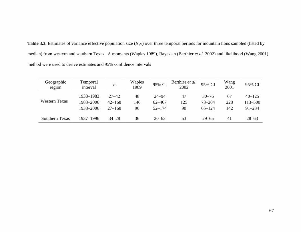
67

Table 3.3. Estimates of variance effective population size (NeV) over three temporal periods for mountain lions sampled (listed by

median) from western and southern Texas. A moments (Waples 1989), Bayesian (Berthier et al. 2002) and likelihood (Wang 2001)

method were used to derive estimates and 95% confidence intervals

Geographic

region

Temporal

interval n

Waples

1989 95% CI

Berthier et al.

2002 95% CI

Wang

2001 95% CI

Western Texas 1938–1983 27–42 48 24–94 47 30–76 67 40–125

1983–2006 42–168 146 62–467 125 73–204 228 113–500

1938–2006 27–168 96 52–174 90 65–124 142 91–234

Southern Texas 1937–1996 34–28 36 20–63 53 29–65 41 28–63

68

Table 3.4. Linkage disequilibrium (Waples 2006) estimates of the effective number of

breeders (Nb) for temporal samples (listed by median) of mountain lions from western

and southern Texas

Geographic region Temporal sample n Nb 95% CI*

Western Texas

1938 27 63 22–∞

1983 42 68 32–544

2006 168 91 65–134

Southern Texas

1937 34 21 12–42

1996 28 9 4–18

*Confidence intervals were computed using a jackknifing procedure.

69

95% CIs for 1937 and 1996 did not overlap means (Table 3.4). Similar to NeV results,

mean Nb for southern Texas was 67–90% lower than western Texas over similar temporal

periods.

Discussion

The demographic history of many species is poorly documented. Thus, a major

challenge in conservation genetic studies is to determine if contemporary levels of

genetic diversity and population structure are the result of recent or historical events. The

initial genetic analyses of Texas mountain lions presented a similar challenge (Walker et

al. 2000). The authors observed low genetic diversity in southern Texas, high structure

between southern and western Texas, but were unable to evaluate alternative hypotheses

without historical samples. Furthermore, the small number of samples (n = 16 and 9 for

southern and western Texas, respectively) limited the inferential power of the analyses.

My diversity estimates in recent western and southern Texas are higher than

reported by Walker et al. (2000), but generally supported their findings in that southern

Texas displayed less diversity. My differing values were likely due to the additional

samples and different loci used in my study. The inclusion of historical samples revealed

a 10–20% temporal decline in diversity for southern Texas. Clearly, the lower diversity

in contemporary mountain lions from southern Texas is a recent phenomenon.

The overall levels of diversity I documented were comparable to other

populations. Estimates for western Texas and historical southern Texas were less than

observed in mountain lions from South America (Culver et al. 2000), but were equivalent

to large and presumably healthy populations in North America (Sinclair et al. 2001;

Anderson, Lindzey & McDonald 2004; McRae et al. 2005). Recent estimates for

70

southern Texas were similar to severely fragmented populations in California, USA

(Ernest et al. 2003).

The genetic differentiation between historical western and southern Texas was

comparable to contiguous populations of mountain lions in western North America

(Sinclair et al. 2001). However, contemporary genetic differentiation between western

and southern Texas was similar to that reported by Walker et al. (2000) and isolated

populations of mountain lions in California (Ernest et al. 2003). The increase in

differentiation over the last 70 years appears to be the result of allele frequency changes

(i.e., genetic drift) that have occurred in southern Texas (temporal FST = 0∙13) rather than

western Texas (temporal FST = 0∙01−0∙03). Small levels of differentiation between

historical southern Texas and the 1983 and 2006 samples from western Texas (FST =

0∙04−0∙05) provide further support for temporal changes occurring mainly in southern

Texas. Indeed, the recent genetic structure observed between mountain lions in southern

and western Texas (Walker et al. 2000) was not present historically.

Estimates of NeV and Nb substantiated my genetic diversity and differentiation

findings. The temporal approach (Waples 1989) revealed similar estimates of NeV in

western Texas over time, and point estimates were similar to other temporally stable

populations of large carnivores (Miller & Waits 2003). Estimates of NeV for southern

Texas were much lower than western Texas providing evidence for a smaller average

population size over time. Estimates of Nb produced results similar to NeV indicating no

population changes over time in western Texas, and a lower average population size in

southern Texas. Estimates of Nb for southern Texas also suggested a decrease over time.

The recent estimate of Nb for southern Texas was 80% lower than the average NeV

71

estimate, and is similar to a reintroduced population of brown bears (De Barbra et al.

2010). The disparity between NeV and Nb estimates is likely because NeV reflects the

harmonic mean over the sampled time period (Waples & Yokota 2007), while Nb

represents the number of breeders producing the sampled cohorts (Waples & Do 2010).

In the case of southern Texas, temporal NeV could have been influenced by larger

historical population sizes whereas, recent estimates of Nb may be indicative of a small

effective size in the contemporary population. This hypothesis was supported by the

temporal decline I observed in genetic diversity within southern Texas.

Historically, mountain lions in western and southern Texas displayed similar

genetic diversity and low genetic structure. Over time, western Texas exhibited

essentially no change in diversity and effective population size, and showed low levels of

temporal genetic differentiation. However, genetic diversity and effective size decreased

to low levels in southern Texas, and temporal genetic differentiation was extensive.

Furthermore, genetic structure has doubled between western and southern Texas over

time. My findings highlight that mountain lions in western Texas have remained

relatively stable over time, but that obvious changes and declines have occurred in

southern Texas.

The human footprint and geographic location may be responsible for the stability

and changes of western and southern Texas. First, urban development and sprawl have

increased dramatically in southern Texas along the Mexico-USA border and in central

Texas. Furthermore, the Rio Grande Valley region of southern Texas supports vast areas

of cropland on both sides of the border. Collectively, development and agriculture have

reduced and fragmented habitat for mountain lions and increased the potential for auto

72

collisions and other mountain lion-humans conflicts in populated regions. Changes in

habitat reducing connectivity could be responsible for the increase in genetic

differentiation for the most peripheral population in southern Texas. In contrast, much of

western Texas remains rangeland with little urban development. The large geographic

area in western Texas, lack of urbanization, and proximity to adjacent mountain lion

populations in New Mexico, USA, and Mexico may have maintained a large effective

size. Movement occurs among western Texas, New Mexico and probably Mexico

(Chapter II), and the population boundaries of western Texas could easily extend beyond

state borders.

Second, during late 1800–mid 1900 livestock production was the dominant

industry in Texas (Lehmann 1969). Predator control was widely practiced to support

livestock production, and predator removals included mountain lions (Wade et al. 1984).

I found no evidence of decline in effective population size for western Texas, but

predator control may have reduced effective size and genetic diversity in southern Texas;

particularly if predator control contributed to isolation from neighboring populations.

Finally, the range of mountain lions contracted during the 1900s due to habitat alteration

and predator control, leaving the southern Texas population isolated on the eastern

periphery of the former range. Location on the landscape has been shown to influence

population size and genetic diversity in species of carnivores (Schwartz et al. 2003).

Peripheral populations may display smaller population sizes, fewer opportunities for gene

flow and greater fluctuations in population size due to geographic range shifts (Schwartz

et al. 2003). Compared to western Texas, southern Texas exhibited lower historical

effective sizes indicating southern Texas may have exhibited peripheral characteristics by

73

the early 1900s. Thus, the temporal decline in diversity and effective size within

southern Texas could be due to population isolation, range contraction, and mortality due

to predator control and other interactions with humans.

CONSERVATION AND MANAGEMENT IMPLICATIONS

My results demonstrate the utility of applying a retrospective genetic approach

(Schwartz, Luikart & Waples 2006) to evaluate the demographic history of an elusive

carnivore. Although exposed to unlimited hunting and a history of land-use change and

persecution mountain lions in western Texas appear to have remained at high and stable

levels. The current level of harvest may not have a large negative effect on the

population. However, my analyses offer no insight on the consequences of increasing

harvest in western Texas, which could easily be realized under current regulations.

Additionally, it is possible that genetic connectivity to adjacent populations is assisting

the stability I observed in western Texas. Connectivity to proximate populations should

be considered when applying habitat or population prescriptions. Future research

examining mountain lion survival and movements in western Texas would inform

questions regarding harvest mortality and interpopulation connectivity. Given the current

information, implementing a monitoring program using indices such as harvest reports

(Anderson & Lindzey 2005) with genetic sampling would be prudent for future mountain

lion management and conservation in western Texas.

Declines have occurred in genetic connectivity, genetic diversity and effective

population size for mountain lions in southern Texas. In fact the temporal decline in

diversity and current effective size are outside of the ranges suggested for long-term

population persistence (Soule et al. 1986). Furthermore, the decline in diversity within

74

southern Texas was 10–20% of the overall decline observed in Florida panthers (Culver

et al. 2000); a population that has displayed physical symptoms of inbreeding depression

(Roelke, Martenson & O’Brien 1993). Additional loss of diversity may occur through

genetic drift if the high mortality and low productivity previously documented (Harveson

1997) are sustained.

Management actions may be needed if mountain lions are to be maintained in

southern Texas. First, the current population size or trend in southern Texas is unknown.

Population monitoring efforts are needed to estimate reproductive rates, survival and

population viability without management intervention. Reporting mountain lion harvests

in southern Texas would assist monitoring efforts. If current harvest is unsustainable,

regulation of harvest may be needed (Young 2009). A harvest management plan would

allow managers to focus harvest on areas of potential mountain lion-human conflict,

while maintaining survival rates of residents and dispersers at sustainable levels. Unlike

the Florida panther, southern Texas exchanges migrants with neighboring populations in

western Texas, New Mexico (Chapter II) and perhaps Mexico. Successful reproduction

by dispersers would increase genetic connectivity, genetic diversity and effective size; all

of which are characteristic of healthy populations (e.g., Spong, Johansson & Björklund

2000). Overall, it is apparent that conservation programs are likely necessary to ensure

the persistence of mountain lions in Texas. This work illustrates the utility of using

museum collections and current genetic samples to examine population histories of

wildlife that are data deficient and difficult to survey.

75

Acknowledgements

I sincerely thank the National Museum of Natural History, Texas Tech University, Sul

Ross State University, Field Museum of Natural History, and Carnegie Museum of

Natural History for providing access to historical samples. I thank Bill Applegate, Louis

Harveson, Jan Janecka and Jimmy Rutledge for assisting with contemporary tissue

collection. I thank Greta Shuster for allowing access to her lab for historical sample

processing. Eric Redeker provided valuable assistance with GIS. The Houston Safari

Club, Quail Unlimited, South Texas Chapter, and Quail Coalition deserve special thanks

for scholarships. Financial support was provided by the Texas Parks and Wildlife

Department.

References

Allendorf, F.W. (1986) Genetic drift and the loss of alleles versus heterozygosity. Zoo

Biology, 5, 181–190.

Allendorf, F.W. & Luikart, G. (2007) Conservation and the Genetics of Populations.

Blackwell Publishing, Oxford.

Anderson, C.R. & Lindzey, F.G. (2005) Experimental evaluation of population trend and

harvest composition in a Wyoming cougar population. Wildlife Society Bulletin,

33, 179–188.

Anderson, C.R., Lindzey, F.G., Knopff, K.H., Jalkotzy, M.G. & Boyce, M.S. (2010)

Cougar management in North America. Cougar Ecology and Conservation (eds

M. Hornocker & S. Negri), pp. 41–54. University of Chicago Press, Illinois.

76

Anderson, C.R., Lindzey, F.G. & McDonald D.B. (2004) Genetic structure of cougar

populations across the Wyoming basin: metapopulation or megapopulation.

Journal of Mammalogy, 85, 1207–1214.

Barea-Azcon, J.M., Virgos, E., Ballesteros-Duperon, E., Moleon, M. & Chirosa, M.

(2007) Surveying carnivores at large spatial scales: a comparison of four broad-

applied methods. Biodiversity Conservation, 16, 1213–1230.

Berthier, P., Beaumont, M.A., Cornuet, J.M. & Luikart, G. (2002) Likelihood-based

estimation of the effective population size using temporal changes in allele

frequencies: a genealogical approach. Genetics, 160, 741–751.

Boulanger, J., Himmer, S. & Swan, C. (2004) Monitoring of grizzly bear trends and

demography using DNA mark-recapture methods in the Owikeno Lake area of

British Columbia. Canadian Journal of Zoology, 82, 1267–1277.

Casas-Marce, M., Revilla, E. & Godoy, J.A. (2009) Searching for DNA in museum

specimens: a comparision of sources in a mammal species. Molecular Ecology

Resources, 10, 502–507.

Culver, M., Hedrick, P.W., Murphy, K., O’Brien, S. & Hornocker, M.G. (2008)

Estimation of the bottleneck size in Florida panthers. Animal Conservation, 11,

104–110.

Culver, M., Johnson, W.E., Pecon-Slattery, J. & O’Brien, S.J. (2000) Genomic ancestry

of the American puma (Puma concolor). Journal of Heredity, 91, 186–197.

De Barbra, M., Waits, L.P., Garton, E.O., Genovesi, P., Randi, E., Mustoni, A. & Croff,

C. (2010) The power of genetic monitoring for studying demography, ecology

77

and genetics of a reintroduced brown bear population. Molecular Ecology, 19,

3938–3951.

Ernest, H B., Boyce, W.M., Bleich, V.C., May, B., Stiver, S.J. & Torres, S.G. (2003)

Genetic structure of mountain lion (Puma concolor) populations in California.

Conservation Genetics, 4, 353–366.

Excoffier, L. & Lischer, H. (2010) Arlequin suite ver 3.5: a new series of programs to

perform population genetics analyses under Linux and Windows. Molecular

Ecology Resources, 10, 564–567.

Flagstad, Ø., Walker, C.W., Vila, C., Sundqvist, A., Fernholm, B., Hufthammer, A.K.,

Wiig, Ø., Koyola, I., Ellegren, H. (2003) Two centuries of the Scandinavian wolf

population: patterns of genetic variability and migration during an era of dramatic

decline. Molecular Ecology, 12, 869–880.

Glaubitz, J.C. (2004) CONVERT: a user-friendly program to reformat diploid genotypic

data for commonly used population genetic software packages. Molecular

Ecology Notes, 4, 309–310.

Harveson, L.A. (1997) Ecology of a Mountain Lion Population in Southern Texas. Ph.D.

Thesis, Texas A&M University & Texas A&M University-Kingsville.

Harveson, L.A., Tewes, M.E., Silvy, N.J. & Rutledge, J. (1996) Mountain lion research in

Texas: past, present, and future. Proceedings of the Fifth Mountain Lion

Workshop (ed W.D. Padly), pp. 45–54. Department of Fish and Game, California.

Hill, W.G. (1981) Estimation of effective population size from data on linkage

disequilibrium. Genetical Research, 38, 209–216.

78

Holsinger, K.E. & Weir, B.S. (2009) Genetics in geographically structured populations:

defining, estimating and interpreting FST. Nature Reviews Genetics, 10, 639–650.

Hurlbert, S.H. (1971) The nonconcept of species diversity: a critique and alternative

parameters. Ecology, 52, 577–586.

Kalinowski, S.T. (2004) Counting alleles with rarefaction: private alleles and hierarchical

sampling designs. Conservation Genetics, 5, 539–543.

Kalinowski, S.T. (2005) HP-RARE 1.0: a computer program for performing rarefaction

on measures of allelic richness. Molecular Ecology Notes, 5, 187–189.

Krimbas, C.B. & Tsakas, S. (1971) The genetics of Dacus oleae. V. Changes of esterase

polymorphism in a natural population following insecticide control-selection or

drift? Evolution, 25, 454–460.

Leberg, P.L. (2002) Estimating allelic richness: effects of sample size and bottlenecks.

Molecular Ecology, 11, 2445–2449.

Leberg, P.L. (2005) Genetic approaches for estimating the effective size of populations.

Journal of Wildlife Management, 69, 1385–1399.

Lehmann, V.W. (1969) Forgotten legions. Texas Western Press, Texas.

Logan, K.A. & Sweanor, L.L. (2001) Desert Puma: Evolutionary Ecology and

Conservation of an Enduring Carnivore. Island Press, Washington D.C.

Longmire, J.L., Maltbie, M. & Baker, R.J. (1997) Use of lysis buffer in DNA isolation

and its implications for museum collections. Occasional Papers, Museum of

Texas Tech University, 163, 1–3.

79

Luikart, G., Ryman, N., Tallmon, D.A., Schwartz, M.K. & Allendorf, F.W. (2010)

Estimation of census and effective population sizes: the increasing usefulness of

DNA-based approaches. Conservation Genetics, 11, 355–373.

Marsh, D.M. & Trenham, P.C. (2007) Current trends in plant and animal population

monitoring. Conservation Biology, 22, 647–655.

McKelvey, K.S., Von Kienast, J., Aubry, K.B., Koehler, G.M., Maletzke, B.T., Squires,

J.R., Lindquist, E.L., Loch, S. & Schwartz, M.K. (2006) DNA analysis of scat and

hair collected snow tracks to document the presence of Canada lynx. Wildlife

Society Bulletin, 32, 451–455.

McRae, B. H., Beier, P., Dewald, L.E., Huynh, L.Y. & Keim, P. (2005) Habitat barriers

limit gene flow and illuminate historical events in a wide-ranging carnivore, the

American puma. Molecular Ecology, 14, 1965–1977.

Menotti-Raymond, M., David, V.A., Lyons, L.A., Schaffer, A.A., Tomlin, J.F., Hutton,

M.K. & O’Brien, S.J. (1999) A genetic linkage map of microsatellites in the

domestic cat (Felis catus). Genomics, 57, 9–23.

Miller, C.R. & Waits, L.P. (2003) The history of effective population size and genetic

diversity in the Yellowstone grizzly (Ursus arctos): implications for conservation.

Proceedings of the National Academy of Sciences, USA, 100, 4434–4439.

Murphy, K.M. (1998) The Ecology of the Cougar (Puma concolor) in the Northern

Yellowstone Ecosystem: Interactions with Prey, Bears, and Humans. Ph.D.

Thesis, University of Idaho.

Nei, M. (1987) Molecular evolutionary genetics. Columbia University Press, New York.

80

Nei, M. & Tajima, F. (1981) Genetic drift and estimation of effective population-size.

Genetics, 98, 625–640.

Peel, D., Ovenden, J.R. & Peel, S.L. (2004) NeEstimator: Software for Estimating

Effective Population Size, Version 1.3. Queensland Government, Department of

Primary Industries and Fisheries, Brisbane, Australia. Available at:

http://www.dpi.qld.gov.au/28_6908.htm (accessed 29 March 2011).

Pittman, M.T., Guzman, G.J. & McKinney, B.P. (2000) Ecology of the mountain lion on

Big Bend Ranch State Park in Trans-Pecos region of Texas. Texas Parks and

Wildlife Department, Final Report Project Number 86, Texas.

Pollack, E. (1983) A new method for estimating the effective population size from allele

frequency changes. Genetics, 104, 531–548.

Roelke, M.E., Martenson, J.S. & O’Brien, S.J. (1993) The consequences of demographic

reduction and genetic depleation in the endangered Florida panther. Current

Biology, 3, 340–350.

Russ, W.B. (1996) The status of the mountain lion in Texas. Proceedings of the Fifth

Mountain Lion Workshop (ed W.D. Padly), pp. 30–31. Department of Fish and

Game, California.

Schmidly, D.J. (2004) The Mammals of Texas, 6th edn. University of Texas Press, Texas.

Schwartz, M.K., Luikart, G. & Waples, R.S. (2006) Genetic monitoring as a promising

tool for conservation and management. Trends in Ecology and Evolution, 22, 25–

33.

81

Schwartz, M.K., Mills, L.S., Ortega, Y., Ruggiero, L.F. & Allendorf, F.W. (2003)

Landscape location affects genetic variation of Canada lynx (Lynx canadensis).

Molecular Ecology, 12, 1807–1816.

Sinclair, E.A., Swenson, E.L., Wolfe, M.L., Choate, D.C., Gates, B. & Crandall, K.A.

(2001) Gene flow estimates in Utah’s cougars imply management beyond Utah.

Animal Conservation, 4, 257–264.

Soule, M., Gilpin, M., Conway, W. & Foose, T. (1986) The millennium ark: how long a

voyage, how many staterooms, how many passengers? Zoo Biology, 5, 101–113.

Spong, G., Johansson, M. & Björklund, M. (2000) High genetic variation in leopards

indicates large and long-term stable effective population size. Molecular Ecology,

9, 1773–1782.

Tallmon, D.A., Grecovich, D., Waples, R.S., Baker, C.S., Jackson, J., Taylor, B.L.,

Archer, E., Martien, K.K., Allendorf, F.W. & Schwartz, M.K. (2010) When are

genetic methods useful for estimating contemporary abundance and detecting

population trends? Molecular Ecology Resources, 10, 684–692.

Wade, D.A., Hawthorne, D.W., Nunley, G.L. & Caroline, M. (1984) History and status of

predator control in Texas. Proceedings of the Eleventh Vertebrate Pest

Conference (ed D.O. Clark), pp. 122–131. University of Nebraska, Nebraska.

Walker, C.W., Harveson, L.A., Pittman, M.T., Tewes, M.E. & Honeycutt, R.L. (2000)

Microsatellite variation in two populations of mountain lions (Puma concolor) in

Texas. Southwestern Naturalist, 45, 196–203.

Wandeler, P., Hoeck, P. & Keller, L.F. (2007) Back to the future: museum specimens in

population genetics. Trends in Ecology and Evolution, 22, 634–642.

82

Wang, D.Y., Eng, B., Waye, J.S., Dudar, J.C. & Saunders, S.R. (1998) Technical note:

improved DNA extraction from ancient bones using silica-based columns.

American Journal of Physical Anthropology, 105, 539–543.

Wang, D.Y., Woiderski, J.R. & Driver, J.C. (2005) DNA analysis of archeological rabbit

remains from the American southwest. Journal of Archaeological Science, 32,

567–578.

Wang, J.L. (2001) A pseudo-likelihood method for estimating effective population size

from temporally spaced samples. Genetical Research, 78, 243–257.

Wang, J. & Whitlock, M.C. (2003) Estimating effective population size and migration

rates from genetic samples over space and time. Genetics, 163, 429–446.

Waples, R.S. (2006) A bias correction for estimates of effective population size based on

linkage disequilibrium at unlinked gene loci. Conservation Genetics, 7, 167–184.

Waples, R.S. (1989) A generalised approach for estimating effective population size from

temporal changes in allele frequency. Genetics, 121, 379–391.

Waples, R.S. & Do, C. (2008) LDNE: a program for estimating effective population size

from data on linkage disequilibrium. Molecular Ecology Resources, 8, 753–756.

Waples, R.S. & Do, C. (2010) Linkage disequilibrium estimates of contemporary Ne

using highly variable genetic markers: a largely untapped resource for applied

conservation and evolution. Ecological Applications, 3, 244–262.

Waples, R.S. & Yokota, M. (2007) Temporal estimates of effective population size in

species with overlapping generations. Genetics, 175, 219–233.

Weir, B.S. & Cockerham, C.C. (1984) Estimating F-statistics for the analysis of

population structure. Evolution, 38, 1358–1370.

83

Wisely, S.M., Maldonado, J.E. & Fleischer, R.C. (2004) A technique for sampling

ancient DNA that minimizes damage to museum specimens. Conservation

Genetics, 5, 105–107.

Witmer, G.W. (2005) Wildlife population monitoring: some practical considerations.

Wildlife Research, 32, 259–263.

Young, J.H. (2009) Estimating mountain lion population parameters in Texas. Ph.D.

Thesis, Texas A&M University-Kingsville.

Young, J.H., Tewes, M.E., Haines, A.M., Guzman, G. & DeMaso, S.J. (2010) Survival

and mortality of cougars in the Trans-Pecos region. Southwestern Naturalist, 55,

411–418.

Wright, S. (1931) Evolution in Mendelian populations. Genetics, 16, 97–159.

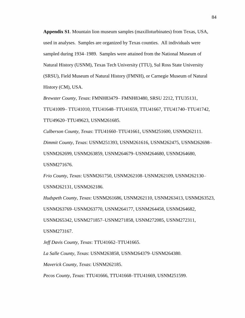
84

Appendix S1. Mountain lion museum samples (maxilloturbinates) from Texas, USA,

used in analyses. Samples are organized by Texas counties. All individuals were

sampled during 1934–1989. Samples were attained from the National Museum of

Natural History (USNM), Texas Tech University (TTU), Sul Ross State University

(SRSU), Field Museum of Natural History (FMNH), or Carnegie Museum of Natural

History (CM), USA.

Brewster County, Texas: FMNH83479– FMNH83480, SRSU 2212, TTU35131,

TTU41009– TTU41010, TTU41648–TTU41659, TTU41667, TTU41740–TTU41742,

TTU49620–TTU49623, USNM261685.

Culberson County, Texas: TTU41660–TTU41661, USNM251600, USNM262111.

Dimmit County, Texas: USNM251393, USNM261616, USNM262475, USNM262698–

USNM262699, USNM263859, USNM264679–USNM264680, USNM264680,

USNM271676.

Frio County, Texas: USNM261750, USNM262108–USNM262109, USNM262130–

USNM262131, USNM262186.

Hudspeth County, Texas: USNM261686, USNM262110, USNM263413, USNM263523,

USNM263769–USNM263770, USNM264177, USNM264458, USNM264682,

USNM265342, USNM271857–USNM271858, USNM272085, USNM272311,

USNM273167.

Jeff Davis County, Texas: TTU41662–TTU41665.

La Salle County, Texas: USNM263858, USNM264379–USNM264380.

Maverick County, Texas: USNM262185.

Pecos County, Texas: TTU41666, TTU41668–TTU41669, USNM251599.

85

Presidio County, Texas: CM21404, CM21406, TTU41670–TTU41677, USNM263772–

USNM263773, USNM271675.

Terrell County, Texas: SRSU 2869.

Val Verde County, Texas: USNM261614.

Webb County, Texas: USNM251375, USNM251418, USNM251468–USNM251469,

USNM261615, USNM263775–USNM263776, USNM263860, USNM264178–

USNM264180, USNM264678, USNM272086, USNM272310, USNM272350.

86

VITA

Name: Joseph Dale Holbrook

Education: B.S., Wildlife Resources, University of Idaho

Address: 725 East Hoffman Ave, Kingsville, Texas 78363

Professional Experience:

2009–Present Graduate Research Assistant, Caesar Kleberg Wildlife Research Institute,

Texas A&M University–Kingsville, Kingsville, Texas

2007–2008 Undergraduate researcher, Laboratory for Ecological and Conservation

Genetics, University of Idaho, Moscow, Idaho

2004–2008 Lead Wildlife Technician (Seasonal), United States Forest Service, Boise

National Forest, Boise, Idaho