Evaluating a hydrological flood routing function for...
82
Evaluating a hydrological flood routing function for implementation into a hydrological energy model 2012-03-16 ___________________________________________________________________ Victor Pelin Alexander Påhlsson Examensarbete TVVR 11/5010 Division of Water Resources Engineering Department of Building and Environmental Technology Lund University
-
Upload
phamkhuong -
Category
Documents
-
view
230 -
download
0
Transcript of Evaluating a hydrological flood routing function for...

Evaluating a hydrological flood routing function for implementation into a hydrological energy model
2012-03-16
___________________________________________________________________
Victor Pelin Alexander Påhlsson
Examensarbete
TVVR 11/5010
Division of Water Resources Engineering
Department of Building and Environmental Technology
Lund University

ii
Abstract In 2011 the Bonneville Power Administration (BPA) released new data for the streamflow in the
Columbia River. This extends the previous database record (1928-1999) to include the last nine years
(1999-2008). Thomson Reuters Point Carbon are using this database to apply their proprietary
hydrological HBV-type energy model in the Columbia River and therefore need a complete
understanding of the data and the methods behind them.
This master thesis aims at understanding the different aspects of hydrological routing in general and
more specifically in the Columbia River and to develop a hydrological routing function. The routing
function should be simple yet robust and applicable in areas where data is scarce.
A routing routine based on the ”cascade of reservoir” routing technique, similar to the one used in the
SSARR model, is developed. The routine is verified by using the parameter values and the average
daily unregulated routed flow (ARF) data provided by the BPA. A methodology for parameter
estimation, in Columbia River and in the general case, is developed. For the general case where the
parameters are unknown, two alternative parameters estimation methods are presented, one method
that can be used with a scarce amount of data and a second one for when additional data is available.
The overall effects of routing in the Columbia River catchment are relatively small. There are apparent
lag times of around 2-3 days and noticeable flow attenuation between the dams Mica (headwaters) and
The Dalles (distance 1300 km). Most of the water in the Columbia River enters as tributaries or local
inflows along the flow path; this reduces the effects of routing at The Dalles. The reasonableness of
the routing routine is evaluated with the Muskingum method. The Muskingum parameter values are
calibrated to fit the effects of routing between Mica and The Dalles, produced by the routing routine.
The calibrated Muskingum parameters are evaluated and considered to be reasonable.
Keywords: Hydrological routing, cascade of reservoirs, Columbia River, Muskingum

iii
Sammanfattning 2011 släppte Bonneville Power Administration (BPA) uppdaterade flödesdata för Columbia River.
Den nya databasen förlänger den tidigare (1928-1999) så att den nu även inkluderar de senaste nio
åren (1999-2008). Thomson Reuters Point Carbon använder denna databas för att applicera sin HBV-
baserade energimodell i Columbia River och behöver därför en full förståelse för data och
bakomliggande metoder.
Målet med detta examensarbete är att få förståelse för de olika aspekterna av hydrologisk routing i
allmänhet och mer specifikt i Columbia River och att utveckla en hydrologisk routing-funktion.
Routing-funktionen ska vara enkel och robust samt tillämpningsbar i områden där tillgången till data
är begränsad.
En routing-rutin baserad på ”cascade of reservoirs” routing-metoden, liknande den som används i
SSARR-modellen, utvecklas. Rutinen verifieras med hjälp av parametervärdena och de dagliga
oreglerade routade medelflödena från BPA. En metod för att uppskatta parametrarna, i Columbia
River och i det allmänna fallet, utvecklas. För det generella fallet då parametrarna är okända,
presenteras två alternativa metoder, en metod som kan användas vid begränsad datamängd och en som
kan användas när mer data finns tillgänglig.
De övergripande effekterna av routing i Columbia Rivers avrinningsområde är förhållandevis små. Det
finns tydliga tidsfördröjningar på 2-3 dagar och en märkbar utjämning av flödet mellan Mica
(källflöde) och The Dalles (avstånd 1300 km). Det mesta av vattnet i Columbia River rinner till som
biflöden eller lokala tillflöden längs med flodsträckan, vilket reducerar effekterna av routing vid The
Dalles. Rimligheten i routing-rutinen utvärderas med hjälp av Muskingum –metoden. Värdena på
Muskingum-parametrarna kalibreras för att passa effekterna av routing, genererade av routing-rutinen,
mellan Mica och The Dalles. De kalibrerade Muskingum-parametrarna utvärderas och anses rimliga.
Nyckelord: Hydrologisk routing, cascade of reservoirs, Columbia River, Muskingum

iv
Acknowledgements We would like to thank our supervisors Dr. Rolf Larsson at Water Resource Engineering (Lund
University) and Stefan Söderberg at Thomson Reuters Point Carbon for valuable comments and
guidance throughout this thesis project. Thank you Rolf for always taking the time to answer and
discuss our questions and sorry for always showing up five minutes early to our meetings. Thank you
Stefan for our interesting meetings and for giving us the opportunity to make this thesis.
To our friends and families, we are thankful for your support and encouragement through rain and
shine. Lastly, we would also like to express our gratitude to Prof. Magnus Larson at Water Resource
Engineering (Lund University) for helping us with contact information.
v
Acronyms and unit converter Station acronym Full station name
ALF Albeni Falls
ARD Hugh Keenleyside
BDY Boundary
BOX Box Canyon
CHJ Chief Joseph
CIB Columbia River at international border
CP Control Point used for routing, at Pasco, WA
GCL Grand Coulee
IHR Ice Harbor
JDA John Day
MCD Mica
MCN McNary
MUC Murphy Creek
PRD Priest Rapids
RIS Rock Island
RRH Rocky Reach
RVC Revelstoke
SEV Seven Mile
TDA The Dalles
WAN Wanapum
WAT Waneta
WEL Wells
YAK Yakima River
Data ID Explanation Unit
A Average daily project inflow cfs
ARF Average daily unregulated routed
flow
cfs
H Average daily observed streamflow
or project outflow
cfs
L Average daily local flow (between
two adjacent stations or projects)
cfs
S Average daily observed storage
change at project site
cfs
Acronym Full name
BPA Bonneville Power Administration
HBV Hydrologiska Byråns Vattenbalansavdelning
SMHI Swedish Meteorological Hydrological Institute
SSARR The Stream-flow Synthesis and Reservoir Regulation
Model
USACE U.S. Army Corps of Engineers
USBR U.S. Bureau of Reclamation
USGS U.S. Geological Survey
US units Metric units
1 ft 0.305 m
1 ft3/s (cfs) 0.0283 m
3/s
3.28 ft 1 m
35.3 ft3/s (cfs) 1 m
3/s
1 mile 1.61 km
0.621 mile 1 km

vi
Table of Contents Abstract ................................................................................................................................................... ii
Sammanfattning...................................................................................................................................... iii
Acknowledgements ................................................................................................................................ iv
Acronyms and unit converter .................................................................................................................. v
1. Introduction ......................................................................................................................................... 1
1.1 The importance of rivers in the hydrological cycle ....................................................................... 1
1.2 Rivers in hydrological rainfall-runoff models ............................................................................... 2
1.3 Developing a simple streamflow routing routine – incentives for this thesis ................................ 2
1.4 Objectives, scope and limitations .................................................................................................. 3
2. Background ......................................................................................................................................... 4
2.1 Streamflow modeling .................................................................................................................... 4
2.1.1 Basic concepts and principles ................................................................................................. 4
2.1.2 Rainfall-runoff modeling ........................................................................................................ 6
2.1.3 Streamflow routing ................................................................................................................. 7
2.1.4 Alternative routing methods ................................................................................................. 10
2.1.5 Routing in the HBV model ................................................................................................... 12
2.1.6 Routing in the SSARR model ............................................................................................... 12
2.1.7 Advantages and disadvantages of hydrologic modeling ...................................................... 12
2.2 Site description – Columbia River .............................................................................................. 13
2.2.1 Description of the catchment ................................................................................................ 13
2.2.2 Bonneville Power Administration (BPA) data ..................................................................... 13
3. Method .............................................................................................................................................. 16
3.1 Cascade Reservoir ....................................................................................................................... 16
3.1.1 Derivation of one reservoir ................................................................................................... 16
3.1.2 Model parameters and computational time step ................................................................... 17
3.1.3 Interpolation ......................................................................................................................... 19
3.2 Applying the model in the general case ...................................................................................... 20
3.2.1 Approximation of model parameters .................................................................................... 20
3.3 Applying the model in Columbia River ...................................................................................... 22
3.3.1 Model verification ................................................................................................................ 22
3.3.2 Lumping channel sub-stretches ............................................................................................ 23
3.4 Optimizing model parameters ..................................................................................................... 24
3.4.1 Sensitivity analysis ............................................................................................................... 24
3.4.2 Objective functions ............................................................................................................... 24
3.4.3 Calibration ............................................................................................................................ 25

vii
3.5 The importance of routing ........................................................................................................... 26
3.6 Comparison with Muskingum routing ......................................................................................... 27
3.6.1 Derivation of Muskingum routing equation ......................................................................... 27
3.7 Computer hardware and software ................................................................................................ 27
3.7.1 Computer hardware .............................................................................................................. 27
3.7.2 Computer software ............................................................................................................... 28
4. Results & Discussion ......................................................................................................................... 29
4.1 Solution procedure using the cascade3 routing routine ............................................................... 29
4.2 Model verification ....................................................................................................................... 30
4.2.1 Rock Island to Wanapum (distance 60 km) .......................................................................... 30
4.2.2 Grand Coulee to Priest Rapids (distance 310 km) ................................................................ 31
4.2.3 Albeni Falls to Grand Coulee (distance 360 km) ................................................................. 33
4.2.4 Mica to The Dalles (distance 1300 km)................................................................................ 35
4.3 Effects of routing ......................................................................................................................... 38
4.3.1 Grand Coulee to Priest Rapids (distance 310 km) ................................................................ 38
4.3.2 Albeni Falls to Grand Coulee (distance 360 km) ................................................................. 39
4.3.3 Mica to The Dalles (distance 1300 km)................................................................................ 41
4.4 Applying the model in Columbia River – Lumped parameters ................................................... 43
4.4.1 Lumping known parameter values ....................................................................................... 43
4.4.2 Parameter values and resulting routing effects Mica to The Dalles ..................................... 43
4.5 Applying the model in the general case ...................................................................................... 45
4.5.1 Scarce amount of data .......................................................................................................... 45
4.5.2 Additional amount of data .................................................................................................... 47
4.5.3 Combination scarce amount of data and additional data ...................................................... 49
4.5.4 Summary of parameter values and resulting routing effects Mica to The Dalles................. 49
4.6 Sensitivity analysis ...................................................................................................................... 53
4.7 Calibrating the model .................................................................................................................. 54
4.8 The importance of routing in hydrological models ..................................................................... 56
4.8.1 No sub reaches ...................................................................................................................... 56
4.8.2 Two sub reaches ................................................................................................................... 57
4.8.3 Four sub reaches ................................................................................................................... 58
4.8.4 Summary of the results of the objective functions ............................................................... 59
4.9 Comparison with Muskingum routing ......................................................................................... 60
4.10 Issues with the Bonneville Power Administration dataset ........................................................ 61
4.11 Suggestions for further studies of the cascade3 routing routine ................................................ 63
5. Conclusion ......................................................................................................................................... 64

viii
6. References ......................................................................................................................................... 65
7. Appendix A. Routing specifics.......................................................................................................... 67
8. Appendix B. MATLAB code ............................................................................................................ 68
The MATLAB code of the cascade3 routing routine ........................................................................ 68
The MATLAB code of the r2 routine ................................................................................................. 70
The MATLAB code of the Qav routine .............................................................................................. 71
The MATLAB code for a routing example ....................................................................................... 72
The MATLAB code of the Muskingum routing routine ................................................................... 73
Statement of contribution
Alexander has written most of chapter 2.2 and Victor has written the main part of chapter 2.1.3. The
rest has been written by both authors. It is the authors’ opinion that both of authors have contributed
equally to this master thesis.

Victor Pelin & Alexander Påhlsson 2012-03-01
1
1. Introduction
1.1 The importance of rivers in the hydrological cycle The ever ongoing circulation of water in different forms between the atmosphere and the land surfaces
or oceans, a concept called the hydrologic cycle, was the starting point for the science of hydrology
(Chow, et al., 1988). Dating as far back as hundreds of year B.C. the Greek philosopher Theophrastus
(c. 372-287 B.C.) managed to correctly describe the hydrological cycle in the atmosphere, with a
sound explanation of how precipitation was formed by condensation and freezing (ibid.). His theory
was later extended by the Roman architect and engineer Vitruvius, around the time of Christ, to
include the explanation that groundwater was mainly derived from precipitation that infiltrated the
ground surface (ibid.). Their work can be seen as a predecessor to the modern version of the
hydrological cycle (ibid.).
The hydrological cycle (see Figure 1) describes the continuous cycling and interdependence of all
phases of water, i.e. gaseous, liquid and solid (Ward and Robinson, 2000). The precipitation that falls
out of the atmosphere can have many different fates, e.g. it can be intercepted by the canopy before it
reaches the ground and then evaporated or it can hit the ground and form surface runoff that eventually
ends up in a nearby stream. The stream then runs out into the ocean or a lake, where water is
evaporated into the atmosphere and forms clouds by condensation, until it finally goes back to being
precipitation again and the circle is complete.
Figure 1: Schematic picture illustrating the hydrological cycle.
In other words, rivers play an important role in the hydrological cycle, receiving water that originates
from overland flow (Qo), throughflow (Qt), groundwater flow (Qg) and direct precipitation (Qp), see
Figure 2; and subsequently transporting it to the sea (Ward and Robinson, 2000).
Evapotranspiration
from land
Evaporation
from oceans
Precipitation
over land
Precipitation
over oceans
Condensation
Water vapour
Infiltration
Overland flow
Throughflow
Groundwater seepage

Victor Pelin & Alexander Påhlsson 2012-03-01
2
Figure 2: Illustration of a cross-section near a river with different flowpaths.
1.2 Rivers in hydrological rainfall-runoff models Hydrological rainfall-runoff models can be divided, according to how physical processes within the
watershed are modeled, into two categories: conceptual and physically based models. Conceptual
models are based on limited representation of the physical processes that produce the model outputs,
e.g. the drainage basin is represented by a number of different storages. Physically based models are
founded on a more solid understanding of the physical processes (Ward and Robinson, 2000).
Examples of conceptual and physically based models are presented below.
The HBV model is a conceptual rainfall-runoff model that was originally developed by SMHI in 1972
(SMHI, n.d.a). River routing, which is a way of modeling the change in the appearance of the
hydrograph as water moves from an upstream to a downstream location, can be described by the
Muskingum method or simple time lags in the HBV model. The Muskingum method is described
more in detail later and is built upon a simple relationship between storage and the inflow and outflow
hydrograph. Although it is popular and easy to use, Henderson (1966) argues that it is based on a
relationship that is not logically complete.
The Système Hydrologique Européen (SHE) model is a physically based rainfall-runoff model that
was developed collaboratively by the UK Institute of Hydrology (IH), the Danish Hydraulic Institute
(DHI) and the Société Grenoblois d’Étude et d’Applications Hydrauliques (SOGREAH) (Ward and
Robinson, 2000). In MIKE SHE there is a program called MIKE 11 that computes the streamflow in
rivers by using an implicit, 1D, finite-difference formulation. There are many options available for
how river routing can be modeled in this program. The options range from the most advanced case
where the complete non-linear Saint-Venant equations (described more in detail later) are used, to the
most simple case where the Muskingum method is used (no routing is also an option) (Singh &
Frevert, 2005). A disadvantage with the Saint-Venant equations is the demand of a lot of site specific
data to be able to model the watershed.
1.3 Developing a simple streamflow routing routine – incentives for this
thesis The main incentive of this thesis is the potential improvement of an existing conceptual rainfall-runoff
model – the HBV-type energy model used by Thomson Reuters Point Carbon – that can comes from
implementing streamflow routing into the model. In 2011 the Bonneville Power Administration
released new data for the streamflow in Columbia River. Thomson Reuters Point Carbon are using this

Victor Pelin & Alexander Påhlsson 2012-03-01
3
database to apply their proprietary hydrological HBV-type energy model in Columbia River and
therefore need a complete understanding of this data and the methods behind them. Since the model is
currently being run without specifically accounting for streamflow routing, it is vital to understand if
and how streamflow routing affects the model performance and moreover if and how streamflow
routing should be accounted for.
1.4 Objectives, scope and limitations This thesis includes four major parts:
The first part is to unravel and investigate the data set from the Columbia River (US) produced
by the Bonneville Power Administration in 2010 (BPA, 2011).
The second part is to develop a routing routine which can be implemented into an existing
HBV-type model.
The third part is to create a simple methodology for estimating the model parameters, both in
the Columbia River basin, but also in the general case where the available data is limited.
The fourth part is to investigate when it is favorable to include streamflow routing in a
hydrologic rainfall runoff model.
The routing routine will be evaluated on different geographical scales using the Columbia River data
set from BPA.
The aim of this thesis is not to develop a new routing technique; instead it will be based on existing
knowledge in the subject.
This thesis does not include testing the developed routing routine with the Thomson Reuter Point
Carbons HBV-type energy model.

Victor Pelin & Alexander Påhlsson 2012-03-01
4
2. Background
2.1 Streamflow modeling
2.1.1 Basic concepts and principles
Hydrograph
A hydrograph is explained by Chow et al. (1988) as “a graph or table showing the flow rate as a
function of time at a given location on the stream”. Any specific hydrograph is a result of a complex
array of factors summarized by Chow (1959) as “an integral expression of the physiographic and
climatic characteristics that govern the relations between rainfall and runoff of a particular drainage
basin”. Common time scales of hydrographs are for example storm hydrographs where the catchment
response during a single storm is shown and annual hydrographs where effects of the long term water
balance in the catchment are shown (Chow, et al., 1988).
Flow classification
A common way of classifying flow in open-channel hydraulics is by classifying the flow as steady or
non-steady and uniform or non-uniform (Chadwick, et al., 2004). Steady or non-steady refers to if or if
not the channel flow changes over time, and uniform or non-uniform refers to if or if not the channel
flow changes in space along the channel length (Chadwick, et al., 2004). Non-uniform flow can in turn
be classified as gradually or rapidly varied flow depending on how much it changes along the channel
length (Chaudhry, 2007).
Manning’s and Chezy´s formula
The Manning and Chezy formulas are resistance equations for steady, uniform, open channel flow
(Henderson, 1966; French, 1994). They describe how flow velocity depends on channel friction and
slope.
The Chezy formula was developed in 1769 by Antoine Chezy and was originally used for the purpose
of designing a canal in the Paris water supply (Henderson, 1966; French, 1994). The formula can be
derived by combining the force balance of any water element in the channel with dimensional analysis
of the bottom shear stress (Henderson, 1966). It is given by French (1994) as:
√ (1)
where u is the mean flow velocity , C √ is a resistant coefficient, R is the hydraulic
radius and S is the bottom slope.
The Manning formula was developed by Robert Manning in 1889 and was based on empirical curve
fitting (French, 1994; Chow, et al., 1988). The formula can be written as (French, 1994):
(2)
where n
is the Manning roughness coefficient. The Manning formula is widely used, because
of its simplicity and reliability, and the Chezy formula is still used in some European countries
(Henderson, 1966; Gordon, et al., 2004).
Continuity equation
The conservation of mass principle is simple and is regarded as the most useful physical principal in
hydrologic analysis. Equations expressing this conservation principle, so called “continuity

Victor Pelin & Alexander Påhlsson 2012-03-01
5
equations”, can be developed for a fluid volume, flow cross-section, and a point within a flow (Chow,
et al., 1988).
Figure 3: Definition sketch for the continuity equation.
An example of where the continuity principle can be applied is that of a river stretch with a changing
water-surface level (Henderson, 1966). Consider the river section shown in Figure 3 with a section of
a very short length, . The discharges at the two ends (Q1, Q2) do not have to be the same and will
differ according to equation 3:
(3)
The term on the right-hand side of equation 3 gives the rate at which the volume within this region is
decreasing. If h is the height of the water surface above a certain datum level, then the volume of water
in the section with length is increasing with a rate according to (Henderson, 1966):
where B is the water surface width. The two terms that were presented in the expression above and
equation 3 must be equal in magnitude but with opposite signs, which together result in the equation of
continuity for unsteady open channel flow (Henderson, 1966):
(4)
This equation is later used in the chapter about hydraulic routing where it has been rewritten by
expanding the term ⁄ ⁄ , which results in (Henderson, 1966):
(5)
where v is the flow velocity of the water, y is the water depth and A is the cross-sectional area.
Momentum equation
The momentum equation describes the unsteady non-uniform open channel flow and is not as easily
derived as the continuity equation described above. The derivation starts with the equation (equation
6) describing the gradient of the total energy line (Henderson, 1966):

Victor Pelin & Alexander Påhlsson 2012-03-01
6
(
) (6)
where H is the height of the total energy line above a certain datum level, h is the height of the water
surface above the same datum level and v is the velocity of the water. From there it is further rewritten
until it finally becomes:
(7)
The interested reader can find the complete derivation of the momentum equation (equation 7) in the
book “Open Channel Flow” by Henderson (1966).
2.1.2 Rainfall-runoff modeling
HBV
The Hydrologiska Byråns Vattenbalansavdelning (HBV) model is a rainfall runoff model developed
by Bergström for the Swedish Meteorological and Hydrological Institute (SMHI) in the early 1970s
(Bergström, 1976; SMHI, n.d.b; Lindström, et al., 1997; Hasan & Elshamy, 2011). The model was
originally developed for runoff simulation and hydrological forecasting in Scandinavian countries, but
has had an increasing range of applications (Lindström, et al., 1997). It has been applied in more than
40 countries all over the world with varying climatic conditions and on scales ranging from small
lysimeter plots to the entire Baltic Sea drainage basin (SMHI, n.d.b).
Many versions of the HBV model have been produced around the world since it was first developed in
the 1970s (Lindström, et al., 1997). The HBV model used by the SMHI is a semi-distributed model,
where the modeled catchment can be divided into several sub basins (SMHI, n.d.b). Each sub basin is
then described according to land use, lake area percentage and elevation (ibid.). The HBV model is
based on conceptual descriptions of a few main features of the hydrological cycle. In its standard form,
it comprises of three major parts: A snow routine, a soil moisture routine and a runoff response routine
(Amenu & Killingtveit, 2001). The snow routine handles snow melt and snow accumulation, the soil
moisture routine handles precipitation and evapotranspiration and computes the storage of water in the
soil, and the runoff routine transforms the percolation from the soil moisture routine into different
levels of runoff (Amenu & Killingtveit, 2001; SMHI, n.d.b). The model is usually run on a daily or
monthly time scale (SMHI, n.d.b; Hasan & Elshamy, 2011).
The HBV model is used for a wide range of applications, from flood forecasting in Nordic countries,
to evaluating climate change scenarios and nutrient load estimates (SMHI, n.d.b).
SSARR
The Stream-flow Synthesis and Reservoir Regulation Model (SSARR) was initially developed for the
North Pacific Division of the U.S. Army Corps of Engineers (USACE) to aid them in their planning,
design, and operation of water control works (USACE, 1991). It has been in the process of
development and application since 1956 and has been applied to numerous river systems in the United
States and elsewhere (ibid.).
It is a numeric model that describes the hydrology of a river catchment system and consists of two
”models”; a watershed model and a streamflow and reservoir regulation model (USACE, 1991). The
watershed model simulates rainfall-runoff, snow accumulation and snowmelt-runoff (ibid.). The
streamflow and reservoir regulation model – which uses a routing technique called the ”cascade of
linear reservoirs”– routes the water in the river from an upstream location to a downstream location
Victor Pelin & Alexander Påhlsson 2012-03-01
7
through channel and lake storage, and is also able to simulate flow through man-made reservoirs
(ibid.). In addition, there is also an option to include effects of backwater, diversion and overbank
flows (ibid.). The SSARR MODEL is able to simulate with time increments that are between 0.1 and
24 hours long (ibid.).
The SSARR model is used by the BPA, the USACE, and the U.S. Bureau of Reclamation (USBR) to
perform a number of studies, e.g. hydro-regulation studies of the Columbia River basin (BPA, 2011).
The SSARR model, in which the cascade routing routine is included, is used as a tool for both
forecasting and long term hydrology studies. Examples of applications are (USACE, 1991):
Simulation of design storms
Daily streamflow forecasting at many points throughout a river system
Seasonal streamflow forecasting.
The model has been developed to be used in relatively large drainage basins with limited amounts of
available observed data, but has been applied to a wide variety of large and small catchments around
the world (USACE, 1991). One specific case where the SSARR model should not be used is for
studies of small drainage areas in urban hydrology since it is a conceptual model rather than a
hydraulic model (ibid.). Also, the minimum computation step is one tenth of an hour, which can be too
long to be able to accurately simulate runoff peaks from very small areas (ibid.).
2.1.3 Streamflow routing
Hydrologic routing
As the flow through a water body changes due to any kind of disturbance, so does the water level and
thereby the water storage in the water body. The change in flow over time can be visualized in a
hydrograph and seen as a flood wave that propagates in the direction of the flow. The hydrograph will,
depending on the properties of the reservoir or channel, change as it propagates. Describing this
change of the hydrograph along the water course is referred to as routing the flow along its course. The
routing is often divided into two effects, time lag and flow attenuation. The time lag refers to the time
lag between two hydrographs caused by the fact that it takes time for a water volume to travel from an
upstream location to a downstream location. The attenuation refers to the change in the shape of the
hydrograph as it propagates caused by the storage capacity of the reservoir or friction and irregularities
of a channel reach (Henderson, 1966; Subramanya, 2008). Hydrologic routing is based on the simple
concept of continuity, which means that the change in storage S over time t in a water body equals the
difference between the inflow I and the outflow O (Chow, et al., 1988):
(8)
If the inflow hydrograph to a water body is known, two unknowns in the equation above remain. This
means that in order to solve the continuity equation, a second equation is required. For this reason a
storage function that relates storage to outflow and inflow is introduced (Chow, et al., 1988).
Hydrologic reservoir or lake routing
In order to solve the continuity equation (equation 8) a second relation between storage and flow is
required. One type of routing is when a flood wave passes through an unregulated lake or reservoir.
For a reservoir with an uncontrolled outflow and a level water surface, there is, depending on the
properties of the discharge point, a fixed relation between lake elevation (h) and the outflow from the
lake (Chow, et al., 1988). Thus:

Victor Pelin & Alexander Påhlsson 2012-03-01
8
(9)
As the lake elevation changes, so does, depending on the topographical properties of the lake, the
volumetric storage in the lake (Chow, et al., 1988). Thus:
(10)
Since both storage and outflow are functions of the lake stage, there is an indirect relation between
outflow and storage (Chow, et al., 1988):
(11)
The relation between stage and outflow can sometimes be determined using hydraulic equations. For
example, flow over several types of weirs can be described as (French, 1994):
(12)
where m and C depend on the physical properties of the weir. The relation between stage and storage
can be estimated using topographical maps. For any lake, the storage can be calculated as:
∫
(13)
where the lake area Alake is a function of the lake elevation h. As an example, consider a case where the
lake area doesn’t change as the lake elevation changes, then equation 13 becomes:
(14)
Combining equation 12 and equation 14 yields a relation between storage and outflow as:
(
)
(15)
where both B and C depend on the properties at the outflow point, and shape of the lake. The simplest
reservoir routing is the linear reservoir routing where the storage varies linearly with outflow as
(Chow, et al., 1988):
(16)
where k (s) is a constant parameter that can be determined by calibration. A physical interpretation of
the k parameter is the lake residence time, a definition of residence time can be found in Chow, et al.
(1988).
Hydrologic channel or river routing
In river routing the continuity equation is still valid. However, the storage is no longer solely a
function of reach discharge. As can be seen in Figure 4, two different storages are possible for the
same reach discharge (Qref), one where the flood wave is rising, and one where the flood wave is
falling. Hence the storage in the reach is no longer a unique function of discharge; instead there is a
looped relationship (USACE, 1994).

Victor Pelin & Alexander Påhlsson 2012-03-01
9
Figure 4: Rising and falling floodwave giving rise to a looped discharge-storage relationship.
A way of describing the routing through a river is by dividing the river into a discrete number of
identical cascading reservoirs (see Figure 5), with level pools, where the storage in each sub reservoir
is assumed to be a function of discharge. The storage is still different depending on whether the flood
wave is rising or falling, but the looped storage-outflow relationship of the total reach is improvingly
mimicked as compared to having a single reservoir (see Figure 5) (USACE, 1994). An example of the
cascading reservoir approach is the ”cascade of linear reservoirs” developed by Nash (1957), where
storage in each sub reservoir is assumed to be linearly proportional to the discharge in each sub
reservoir. The ”cascading reservoir” routing technique will be the approach used in this report,
however not with the linear relationship described above, but where the constant term in the linear
relationship is flow dependent.
Figure 5: The channel reach is approximated as a number of equal reservoirs. The storages in two of the reservoirs
with equal discharge are still different, but the error is reduced with increasing number of reservoirs.

Victor Pelin & Alexander Påhlsson 2012-03-01
10
Another popular way of better describing the flow through a river reach is by defining the concepts of
prism and wedge storage as seen in Figure 6 below.
Figure 6: The concepts of wedge and prism storage.
The total storage in the reach is then:
(17)
This can be rewritten in the form known as the Muskingum method (Henderson, 1966):
[ ] (18)
where K is a model parameter often associated to travel time, X is a model parameter that depends on
the wedge properties of the flood wave (Chow, et al., 1988). Hence the storage does now not only
depend on the reach discharge, but on the inflow as well.
2.1.4 Alternative routing methods
Hydraulic routing
Despite the popularity and ease of use of the hydrologic Muskingum routing method, it is as
mentioned previously not logically complete. The equations of motion do not justify the belief that
storage is strictly determined by inflow and outflow alone (Henderson, 1966). A more physical
approach to river routing is to use hydraulic routing techniques, which utilize some form of the
momentum equation to solve the continuity equation. In many cases some terms in the momentum
equation can be neglected, because of their insignificance in comparison to other terms. Below follows
a discussion of three special cases where it is valid to make certain approximations.
Dynamic routing
The equations of motion or the St Venant equations – the continuity and the momentum equation
(equation 5 and equation 7) – solved together with proper boundary conditions are called the complete
dynamic wave equations (USACE, 1994). These equations are considered to be the most accurate
solution to 1-D unsteady flow problems in open channels (ibid.). However, they are based on
assumptions that give rise to limitations of use. The assumptions used to derive the dynamic wave
equations are (ibid.):
i. Velocity is constant and the water surface is horizontal across any channel section.

Victor Pelin & Alexander Påhlsson 2012-03-01
11
ii. All flows are gradually varied with hydrostatic pressure prevailing at all points in the flow,
such that vertical accelerations can be neglected.
iii. No lateral secondary circulation occurs.
iv. Channel boundaries are treated as fixed; therefore, no erosion or deposition occurs.
v. Water is of uniform density, and resistance to flow can be described by empirical formulas,
such as Manning’s and Chezy’s equation.
(19)
(20)
where A is the cross-sectional area, v is the water velocity, B is the width of the river, y is the water
depth, q is the discharge per width of river, Sf is the friction slope (which is the slope of the total
energy line) and S0 is the bottom slope (ibid.). Figure 7 shows a planar and cross-section of a section
of a river where the notations described above are illustrated.
Figure 7: Planar and cross-sectional sketch of river section, with the total energy line (Sf), bottom slope (S0), water
depth (y), river width (B) and cross-sectional area (A).
Kinematic routing
For some flow situations the gravitational and frictional forces approach equilibrium. In such cases,
changes in depth and velocity with respect to time and space are small compared to the bed slope of
the channel (USACE, 1994). This justifies a deletion of the acceleration terms – both local and
convective – from the full dynamic wave equations (equation 19 and equation 20), which then reduces
to (ibid.): .
This equality between the friction slope and the bottom slope can be utilized in river routing. By
combining Manning’s or Chezy’s equation with the continuity equation, the governing kinematic
wave equation becomes (USACE, 1994):
(21)
where and are terms related to flow geometry and surface roughness. Since the kinematic wave
equation lacks all acceleration terms it assumes steady uniform flow and therefore it does not allow

Victor Pelin & Alexander Påhlsson 2012-03-01
12
hydrograph diffusion (USACE, 1994). In other words, the kinematic wave equation only translates the
hydrograph in time without any attenuation of the peak flow (ibid.).
Diffusion routing
Another approximation of the dynamic wave equations, but one which allows for diffusion of the
hydrograph (unlike the kinematic approximation), is the diffusion wave model. It adds a term for the
pressure differential to the kinematic wave equation (equation 23), which then becomes the diffusion
wave equation (USACE, 1994):
(22)
The pressure differential term allows the diffusion model to describe the attenuation of a flood wave
and also provides a possibility of specifying the boundary condition at the downstream end, to account
for backwater effects (USACE, 1994). Although it does not include the last two inertial terms of the
dynamic wave equation (equation 23), which limits the application to slow and moderately rising
flood waves, it can still describe most natural flood waves (ibid.).
( ) (23)
2.1.5 Routing in the HBV model
An additional part of the HBV model is to include routing. SMHI (n.d.b) mentions the possibility of
describing routing between sub basins by using the Muskingum method or by using simple time lags.
Another option is to entirely skip routing by simply adding the contributions of the different sub basins
(ibid.). As mentioned previously, lake area percentage is determined for all modeled sub basins. This
is because the model also includes level pool lake routing (SMHI, n.d.b; Lindström, et al., 1997).
2.1.6 Routing in the SSARR model
The SSARR model is divided into several sub-models, one of which is the “River and Reservoir
model”. This sub-model routes the streamflow from an upstream point to a downstream point and uses
a routing method referred to as a “cascade of reservoirs” technique (USACE, 1991). The cascade of
reservoirs technique simulates the lag and peak attenuation – the effects of routing – by dividing the
river into successive increments (ibid.). Thus, the river channel can be thought of as a series of small
“lakes” representing the natural delay and attenuation of runoff (ibid.).
2.1.7 Advantages and disadvantages of hydrologic modeling
The major advantage of conceptual hydrologic models as opposed to physical or hydraulic models is
the low demand on the amount of available data. The model parameters have little or no physical
meaning and cannot be measured; instead they are calibrated and validated using measured historic
streamflow. Adapting the model to historic conditions of course brings problems if future conditions
change, as for example if the climate would change. Furthermore streamflow data is often measured or
modeled as daily or monthly average whilst the effects of routing in small catchments, as the reader
will see later in this report, sometimes occur on a much smaller time scale.
Kinematic wave
Diffusion wave
Dynamic wave
Victor Pelin & Alexander Påhlsson 2012-03-01
13
2.2 Site description – Columbia River This thesis is focused on developing a streamflow routing routine, by studying BPA’s “Level
Modified Streamflow” report on the Columbia River Basin. Below follows a short description of the
area and some of the data types produced by BPA.
2.2.1 Description of the catchment
The Columbia River Basin (see Figure 8) stretches over 670,000 km2, including parts of seven U.S.
states and the Canadian Province of British Columbia (USEPA, 2012). Because it covers such a vast
area the climate across the region is variable. Annual precipitation is highest in the mountain areas
(e.g. Coast Mountains and Cascade Ranges) and lowest in the plateau areas (e.g. Columbia and Snake
River Plateau) (BPA, 2011). Temperatures are milder along the coast than inland, and temperature
variations are much more pronounced inland than along the coast (ibid.).
Figure 8: Map of the Columbia River Basin (USACE, n.d.).
The region is situated in a zone of prevailing westerly winds, which brings fronts that are associated
with extensive precipitation (BPA, 2011). The dominating type of runoff divides the region in two: (1)
one snowmelt-dominated regime east of the Cascade Range, and (2) one rainfall-dominated regime
along the coast west of the Cascade Range (ibid.). East of the Cascades the snow melts in May through
July, giving rise to peak streamflow discharges around early June (ibid.). West of the Cascades most
rain falls during the winter months and most of the runoff occurs in the winter period that stretches
from October to March (ibid.).
2.2.2 Bonneville Power Administration (BPA) data
The BPA in conjunction with the U.S. Army Corps (USACE) and the U.S. Bureau of Reclamation
(USBR) releases a “Level Modified Streamflow” report once every ten years. According to BPA
(2011) the definition of modified flows is: “…the historical streamflow that would have been observed
if current irrigation depletions (as of 2008) existed in the past and if the effects of river regulation were
removed (except at Snake, Deschutes, and Yakima basins where current upstream reservoir regulation
practices are included)”.

Victor Pelin & Alexander Påhlsson 2012-03-01
14
This streamflow dataset is, among other things, used for analysis of environmental impacts, power
revenue forecasts, and flood control studies (BPA, 2011). Below follows an explanatory part of the
data types that are of relevance for this thesis.
H
This data type is the average daily observed streamflow or project outflow, which are dams used for
hydropower production (BPA, 2011). For some periods streamflow gaging data was missing, but this
was corrected by using linear regression of the streamflow from nearby gaging stations (ibid.). At
some places the gaging station was not placed at the project, which was corrected by taking the
streamflow from an upstream station and then adding a portion of the incremental flow based on a
drainage area ratio (based on the ungaged portion of the drainage area) (ibid.). Where obvious errors
occur in the data set, linear interpolation between good data points were used instead (ibid.). However,
if large amounts of data were missing, alternative sources had to be used (e.g. stream gage data from
U.S. Geological Survey, USGS) (ibid.).
S
This data type is the average daily observed storage change at project sites, which includes the storage
change that occurs during the initial filling of the project in question (BPA, 2011). As opposed to H
values, S values can have both positive and negative values. The S data was taken from various
sources, e.g. USGS, the USACE, Environmental Canada, and project owners. Missing and erroneous
data was corrected using the same methods described in the section above (ibid.).
A
A is the average daily project inflow and was either calculated by using H and S values for the project
(see equation 24) or given by the project owners (BPA, 2011).
(24)
However, when calculating the project inflow from equation 24, values were sometimes negative
(which in most cases is incorrect). The probable cause of such errors is the S data and this is because
reservoir storage is often determined by storage/elevation tables (BPA, 2011). Due to the large area
that projects usually occupies, small errors in the elevation readings (e.g. caused by wind setup) can
result in large errors in the corresponding storage and change in storage values. These errors were
corrected by increasing the storage change values until a reasonable positive inflow was obtained
(ibid.). In order to preserve the original overall monthly storage change volumes, the same amount of
water that was added to correct the project inflow for one day was subtracted from another day that
month (ibid.).
L
L is the average daily local flow that comes into the river system between two data points, e.g.
between two projects or between a project and a gaging station (BPA, 2011). To retrieve the local
flows it is necessary to route the upstream outflow to the downstream project or gaging station, by
using the Streamflow Synthesis and Reservoir Regulation model (SSARR) (ibid.). An example that
shows how the local flow is calculated between an upstream dam and a downstream gaging station is
shown in equation 25 below (ibid.).
(25)
To check for errors calculated local flows are plotted and studied, in order to determine whether it has
a logical hydrological shape or not. Most of the time, unfortunately, the local flow had erratic spikes or

Victor Pelin & Alexander Påhlsson 2012-03-01
15
negative values (BPA, 2011). Negative values of local flows can be caused by any of the following
reasons: surface water – groundwater interconnections, evaporation, diversionary water uses or
inaccurate project data (ibid.). These negative values were corrected by using a method called
indexing, which is described in the “2010 Level Modified Streamflow” report (ibid.).
ARF
ARF is the average daily unregulated routed flow, which denotes the flow, in a point along the river,
as it would have been if no upstream dams existed (BPA, 2011). ARF is calculated by adding the local
flow between two locations (two dams or a dam and a gaging station) to the inflow (A) into the
upstream dam, routed (by SSARR) down to the downstream location (ibid.). An example of the
calculation procedure, when calculating the ARF value at Revelstoke Dam (which is the first
downstream station from Mica Dam), is shown in equation 26 below. Revelstoke is denoted RVC,
Mica is denoted MCD and the number after the name denotation (in this case 5) shows which revision
of the “Level Modified Streamflow” report that the data originates from (ibid.).
(26)
ARF is the data type that will be used throughout this report, when for example model performance is
evaluated. This is because ARF data is only influenced by routing and therefore was decided to be the
most suitable for this routing study.
Alternative data method
In the mid-Columbia River reach, between the Chief Joseph and the Priest Rapids projects, all project
inflows (A), outflows (H) and local inflows (L) have been recalculated due to problems with negative
locals and odd runoff shapes (BPA, 2011). Since almost all the side streams coming into the river are
gaged, the local inflows have instead been replaced by gaged data from these tributaries (ibid.). The
observed outflow at Chief Joseph and the inflow at Priest rapids have been assumed to be correct
(ibid.). All in-between project inflows have been recalculated by routing the upstream outflow to the
next station and adding the new local inflows (ibid.). Storage data was also assumed to be correct in
order to recalculate the project outflows according to equation 24 above (ibid.).

Victor Pelin & Alexander Påhlsson 2012-03-01
16
3. Method
3.1 Cascade Reservoir
3.1.1 Derivation of one reservoir
A routing equation, for one reservoir, similar to the one used in the SSARR model will be derived
below.
The continuity equation for a river reach can be written as:
(27)
where S is storage, t is time, I and O are inflow and outflow respectively from the river reach. The
above equation is discretized for a finite time increment, ∆t:
(28)
If the inflow and outflow during the time period ∆t are approximated as the mean over the period, the
above equation becomes:
(29)
The storage is assumed to depend on the discharge as (USACE, 1991):
(30)
TS is a proportionality factor between storage and outflow and could be interpreted as the time of
storage (USACE, 1991) i.e. retention time. Inserting equation 30 into equation 29 yields:
(
) (31)
Rearranging and separating all terms related to outflow at t+∆t to one side gives:
(
) (
) (32)
where
. Assuming that and rearranging equation 32 gives:
( (
))
(
)
( (
))
(
)
(33)
The above equation can be rewritten as the final reservoir routing equation (USACE, 1991):
(
)
(34)
The time of storage Ts is assumed to vary with discharge as (Rice & Larson, 1972) (USACE, 1991):
(35)

Victor Pelin & Alexander Påhlsson 2012-03-01
17
where KTS and n are parameters obtained by calibration (USACE, 1991). The mean time of storage
over a time increment ∆t can based on equation 35 be written as:
(( )
) (36)
3.1.2 Model parameters and computational time step
The model parameters will be introduced below, in the subsequent parts of this chapter. The parameter
units are user specified and are therefore only suggestions. Note that in equation 34, the time of
storage and the computational time step have to be of the same unit, e.g. (hours). Also, the inflows and
outflows have to be of the same units, e.g. (m3/s). More physical interpretations and methods of
estimating the parameters will be reviewed later in this chapter. Finally, the computational time step
will be commented on.
The number of sub reservoirs
The number of sub reservoirs affects the attenuation of the discharge, where one single reservoir yields
the greatest level of attenuation and an infinite number of reservoirs cause no flow attenuation, only
translation of the hydrograph (Heatherman, 2008). The optimal number of sub reservoirs is reach
specific and should ultimately be obtained by calibration (USACE, 1994). A rule of thumb presented
by the U.S. Army Corps (USACE) (1994) is that time of storage in each sub reservoir should be less
than 1/5 of the time of rise of the inflow hydrograph (ibid.). Another way of estimating the number of
phases is to introduce the concept of “characteristic reach length” – first developed by Kalinin and
Milyukov in 1958 – which is the conceptual channel length for which there is “a one-to-one
relationship between the depth in the midpoint and the discharge at the downstream end”
(Heatherman, 2008). This relationship also means that there exists a one-to one relationship between
storage in the sub reach and the discharge at the downstream end (ibid.). The SSARR manual suggests
that a crude approximation of the number of sub reservoirs can be obtained by assuming a
characteristic reach length of 5-10 miles (USACE, 1991). The USACE (2000) suggests that the
number of steps can be estimated using the following equation, based on empirical work done by
Strelkoff in 1980:
(37)
where N is the number of steps, L is the total reach length, S0 is the bottom slope and y0 is the normal
flow depth at base flow (Heatherman, 2008). A similar equation can be formulated based on the
derivation of the characteristic reach length derived by Perumal (1992) (Heatherman, 2008):
(38)
where Lu is the characteristic reach length, Q0 is discharge, T is the top width, C0 is the wave celerity at
the reference discharge Q0. Dividing the total reach length by the characteristic reach length gives the
number of required sub reservoirs:
(39)
The parameter value of the number of sub reservoirs is an integer value exceeding or equal to1.

Victor Pelin & Alexander Påhlsson 2012-03-01
18
The KTS parameter
The KTS parameter (h*(m3/s)
n) linearly affects the time of storage in the sub reservoirs (see equation
35). A large KTS thus results in a large time of storage and vice versa. Since a negative time of storage
is unrealistic, the KTS parameter has to be positive. KTS includes several physical properties of the
river reach such as friction, geometry, length and slope (Tingsanchali, 1986).
The n parameter
The time of storage changes with different discharge according to equation 35. Hence Ts in equation
34 includes a dependence of the discharge. Whether the time of storage increases or decreases with
discharge depends on the flow situation and is regulated by the exponential coefficient n. The range of
the n parameter is according to USACE (1991) between -1 and 1.
Time of storage varies with discharge according to equation 35, where the n coefficient controls the
impact that a change in discharge has on the time of storage. In other words, it is a coefficient which
controls the linearity/non-linearity of time of storage, where the linearity increases as n decreases and
vice versa when n increases.
Normally when streamflow is restricted to the channel, the time of storage varies inversely with
discharge, in which case n becomes a positive number (USACE, 1991). This is intuitive since with a
higher discharge the water stays within a particular stream reach for a shorter amount of time than
compared to a case with lower discharge. Figure 9 shows how the time of storage varies for different
discharge values when n=-0.2, n=0, n=0.2 and n=0.4 respectively. The n coefficient, as mentioned
before, usually has a value that is between -1 and 1 (ibid.).
Figure 9: Time of storage plotted against Q for different values of n.
Sometimes it may be necessary to use negative values for n, which means that time of storage instead
varies directly with the discharge. In this case an increase in discharge means an increase in time of
storage (USACE, 1991). In order to explain such a relationship between discharge and time of storage
consider a stream reach where overbank flow is dominant, when discharge increases the stream
expands laterally onto its floodplains and the flow slows down markedly, thus increasing the time of
storage of the water. Figure 9 shows how the time of storage varies for different discharge values
when n=-0.2.
Tim
e o
f st
ora
ge (
Ts)
Discharge (Q)
How time of storage changes with discharge and n
n=0.4
n=0.2
n=0
n=-0.2

Victor Pelin & Alexander Påhlsson 2012-03-01
19
Time of storage is affected to a relatively large extent by the value of n. Smaller values of n yields a
greater time of storage, assuming KTS to be constant for changes in n, and vice versa (USACE, 1991).
The total time of storage
All the above parameters combine into the flow dependent time of storage per phase (see equation 35).
Depending on the n parameter, the time of storage will either increase or decrease with flow. The total
time of storage in the reach will affect both attenuation and the lag time, where a large time of storage
will cause more attenuation and a larger time lag, and vice versa.
The computational time
It is intuitive that a too large computational time step as compared to the time of storage, will affect
the routing results negatively. In fact, as the computational time approaches two times the time of
storage in equation 34, the outflow is less and less affected by the outflow at the previous time step. If
the computational time step equals two times the time of storage, then the outflow (at t+ t) is simply
just the average of the inflow (at t and t+ t) as equation 34 becomes:
( )
→
If the computational time step increases even further, the equation above will produce a negative effect
of the outflow at the previous time step. In the limit where the computational time step approaches
infinity, equation 34 becomes:
( )
→
It is reasonable that as the computational time step increases, what happened at the previous time step
has less and less effect on what is happening on the current time step. It is however not reasonable that
what happened at the previous time step can affect the current time step negatively. Furthermore, the
above equation could potentially produce negative outflows if Ot>2*Im. Therefore, the value of the
computational time step should never exceed two times the minimum value of time of storage.
3.1.3 Interpolation
If the input data is of a cruder time resolution than the computational time step, the program has to
interpolate the data between known data values. In the BPA data set, the input data is daily average at
the finest. If the computational time step is set to for example 1 hour, the daily averages have to be
interpolated to give data over all of the 24 hours of the day. In the cascade3 routing routine – which is
the name of the routing routine that is developed in this thesis – daily average values are set to
represent all the sub time steps of the day, giving rise to a step-wise appearance of the hydrograph, as
can be seen in Figure 10.

Victor Pelin & Alexander Påhlsson 2012-03-01
20
Figure 10: A solution matrix from the cascade3 routing routine. The blue line shows the "constant" interpolation.
3.2 Applying the model in the general case
3.2.1 Approximation of model parameters
If no model parameters are available, a general method of estimating the parameters is needed. The
simplest method is to use parameters from similar areas, if available. Otherwise, the following
methods can be used.
The n parameter
The residence time of a water body is by definition the volume of the water body divided by the
throughflow (Chow, et al., 1988):
(40)
If the water body is a channel reach of a certain length L and a cross sectional area A, the above
equation can be rewritten as:
(41)
It is obvious that the cross sectional area will vary with the flow. For uniform steady flow, this can be
described using the Manning formula (French, 1994):
(
)
(42)
Assuming a wide channel (B>>y), and rearranging the above equation, the cross sectional area can be
expressed as a function of the flow:
(
)
(43)
Inserting equation 43 into equation 41 gives:
(44)

Victor Pelin & Alexander Påhlsson 2012-03-01
21
The above equation confirms what is intuitive, that the time of storage increases with increasing
friction, and decreases with increasing slope. Furthermore it provides an estimate of the n parameter of
0.4.
The nbrPhases parameter
The nbrPhases parameter represents the number of sub reservoirs, or phases, that the total river reach
is divided into. The nbrPhases parameter can be estimated with different methods depending on the
amount of data available. The simplest way of estimating the parameter is by using the rule of thumb
from the SSARR manual, previously mentioned as (USACE, 1991):
(45)
where the unit of Lreach is expressed in km.
If more reach data is available, equation 37 or equation 39 can be used to estimate the parameter:
(37)
(39)
where Lreach is the total reach length, y0 is the water depth at base flow, C0 is the flood wave velocity at
the reference flow, T is the top width, S0 is the bottom slope and Q0 is the reference flow. The
characteristic reach length will be different for different discharges (Heatherman, 2008), which means
that the number of phases will be optimized for the reference flow, Q0. Therefore the mean flow is
used as the reference flow.
It should be kept in mind that the nbrPhases parameter has to be a positive integer value.
The total time of storage Ts
As for the nbrPhases parameter, two different methods, with different level of required data, will be
used to estimate the total time of storage in the river reach. Both methods assume that the time of
storage is approximately the travel time (USACE, 1991) through the reach.
Figure 11: Estimating the travel time by studying inflow and outflow hydrographs at increasing intermediate
distance. This specific peak is around the mean flow of the full hydrographs.
The first and most obvious method is to look at the streamflow data sets, study the inflow and outflow
hydrographs from the river reach and estimate the time lag between the two hydrographs. Since high

Victor Pelin & Alexander Påhlsson 2012-03-01
22
and low flow will pass through the reach at different time of storage (see for example equation 35), it
is suggested to study the hydrographs around the mean flow. A problem arises if the time lag between
the inflow and outflow hydrographs is much less than the time resolution of the hydrograph data. The
strategy to address this issue is then to compare outflow and inflow hydrographs at greater
intermediate distance (see Figure 11) and to increase the intermediate distance until a clear time lag
can be seen. This of course requires data at multiple gaging stations along the river. The time of
storage for the different reaches is then simply determined by dividing the total time of storage
according to the length of the sub reaches. Thus the time of storage for a reach is estimated as:
(46)
The second method for estimating the total time of storage is by estimating the flood wave velocity
through the reach. The flood wave velocity can be estimated to be the mean velocity multiplied by 1.5
(USACE, 1991; USACE, 2000; Rantz, 1982):
(47)
where the mean velocity Umean can be estimated using the Manning formula (see equation 2).
This means that the total time of storage can be approximated as:
(48)
The KTS parameter
The only parameter that remains to be determined in equation 35 is the KTS parameter. This parameter
can be calculated as (USACE, 1991):
(49)
where Ts is the time of storage for the reach and Q is the mean flow through the reach.
3.3 Applying the model in Columbia River The cascade routing routine will be evaluated using the BPA (2011) data from the Columbia River.
The evaluation partly involves verifying the performance of the model and also getting familiarized
with the model and its parameters.
3.3.1 Model verification
To verify the performance of the cascade routing routine,
the routing through Columbia River as performed by the
BPA (2011) will be recreated and compared to the result
from BPA. The data recreated is the ARF data, simply
because they only consider the effects of routing and are
unaffected of further refinements. This involves a stepwise
routing procedure where the river is divided into a number
of sub reaches separated by stations, either dams or gages.
The flow at the headwater is routed to the next following
station and simply added to the local inflow over the sub
reach. This flow is in turn routed to the next station where
the next local inflow is added, and so on (see appendix Figure 12: Maps showing the different
geographic distances. The right hand map is
taken from Google Earth (2011).

Victor Pelin & Alexander Påhlsson 2012-03-01
23
Table 20 and
Table 21 for the exact procedure). This process continues all the way down to a final station where the
recreated ARF data is compared to the ARF data provided by the BPA (2011). The model verification
is in this way a comparison between the recreated routing routine and the routing in the SSARR
model, to confirm that the recreation is successful.
The model verification will be performed on three different geographical scales (Figure 12):
Short distance: The river reach between Rock Island (RIS) and Wanapum (WAN),
approximately 60 km. This particulate reach was chosen for the simplifying property of
having negligible local inflow and thereby only shows the effects of routing.
Intermediate distance: Two different river stretches of approximately the same length but with
different routing parameters. The first one is the part of the river between Grand Coulee
(GCL) and Priest Rapids (PRD), approximately 310 km. The second one is the part of the
river between Albeni Falls (ALF) and Grand Coulee (GCL), approximately 360 km.
Long distance: The part of the river between Mica (MCD) and The Dalles (TDA),
approximately 1300 km.
3.3.2 Lumping channel sub-stretches
This section evaluates the possibility of adding, or lumping, together the parameters from several
reaches into one set of “lumped” parameters for the entire reach. A procedure for how to lump known
parameters is suggested and tested.
Lumping multiple known stream stretch parameters
If the parameter values of nbrPhases, n and KTS are known for a number of succeeding channel sub
stretches, then the parameter values for the total channel stretch (including all sub reaches) can be
estimated as follows.
The nbrPhases parameter
Since all of the sub reaches each has an optimal number of phases, the number of phases for the entire
channel stretch is simply taken as the sum of the number of phases for all the sub reaches:
∑ (50)
where k is the number of sub reaches.
The KTS parameter
The total time of storage for a lumped channel stretch of k number of channel reaches equals the sum
of the time of storage for all the sub reaches:
(51)
If
then the above equation can be rearranged and reduced to:
∑
(52)

Victor Pelin & Alexander Påhlsson 2012-03-01
24
This means that the KTS value for the entire reach can be estimated by weighing the KTS values from
all the sub reaches based on their number of phases.
The n parameter
Taking the logarithm of both sides in equation 51 and rearranging gives:
(
)
(53)
If and if , then (54)
Evaluating the performance of the lumped routing
In order to investigate if the lumped model produces the same routing effects as the stepwise routing, a
stream reach that stretches from Mica (MCD) all the way down to The Dalles (TDA) (see Figure 12),
will be used. The routing effects are first computed by routing the flow from the headwater MCD
stepwise all the way down to TDA without adding the local inflows along the way. The lumped model
is then run using the lumped parameters in one “lumped” step and then compared to the routing effects
from the stepwise routing.
3.4 Optimizing model parameters
3.4.1 Sensitivity analysis
To make the calibration process more effective, it is important to know how the individual parameters
affect the outcome of the model. In the sensitivity analysis all model parameters are modified
individually to check how they affect the model output. One at a time, all of the parameter values are
first reduced to half and then increased to twice their original values, while simultaneously checking
the model output for these new values. This is done to get a better understanding of the model
parameters, so that it is clear how one should modify the parameters in order to optimize the model
performance during calibration.
3.4.2 Objective functions
The objective functions evaluate the model performance, which aids the user in deciding whether the
model output is good or bad. Even if the objective functions give an exact number of the model
performance it is still up to the user to decide if it is acceptable or not, in other words it is a subjective
decision. Below follows a description of two objective functions, one which is used frequently to
evaluate hydrological models and one that was created specifically to evaluate the cascade3 routing
routine.
Nash-Sutcliffe efficiency – r2
Moriasi et al. (2007) describes the Nash-Sutcliffe efficiency (r2) as: “a normalized statistic that
determines the relative magnitude of the residual variance (“noise”) compared to the measured data
variance (“information”)”. The term residual is in this case referring to the “error” in the model result
data as compared to the observed data.
∑ (
)
∑ ( ̅̅ ̅̅ )
(55)
observed discharge

Victor Pelin & Alexander Påhlsson 2012-03-01
25
modeled discharge
⁄ observed/modeled discharge at time t
(Nash and Sutcliffe, 1970)
The r2 value is commonly used to evaluate the performance of conceptual hydrological models.
Acceptable levels of performance are when r2 ranges between 0.0 and 1.0 (Moriasi, et al., 2007).
When r2 values are smaller than 0.0 it is an indication of that the mean observed value gives a better
prediction than the simulated value, which means that the model performance is unacceptable (ibid.).
An r2 value of 1.0 on the other hand indicates optimal model performance (ibid.).
The Nash-Sutcliffe ratio was, as mentioned above, originally intended to evaluate the performance of
conceptual hydrological models. Since streamflow routing only is a part of the hydrological cycle the
use of r2 is not optimal. Therefore, when evaluating the effects of routing, r
2 values will be near to 1.0.
This means that to be able to compare the r2 values from the different river reaches, a high number of
significant digits is needed. In this report, the number of significant digits for r2 will be kept high
enough to show where it deviates from unity.
Mean of the absolute flow error – Qav
The cascade3 routing routine strives to replicate U.S. Army Corps’ (USACE) “cascade of reservoir”
routing function as close as possible, which makes it interesting to compare simulated streamflow,
from USACE’s and the cascade3 routing routine, over time. To get a rough idea of how well the
cascade3 routing routine depicts their model one can sum the difference in streamflow – between the
two models – at each time step, and divide by the number of simulated time steps, which gives the
average flow error of the cascade3 routing routine. However, to avoid the risk of negative flow errors
cancelling out positive errors, it is necessary to take the absolute value of the flow error, before
summing the errors and dividing by the number of time steps. As can be seen in equation 56, the
objective function has the same unit as the discharge and is in other words not normalized. This is
because the effects of routing are a small part in the hydrological cycle, as mentioned in the previous
section, which would result in an insignificantly small value if it was normalized by for example the
total discharge.
∑ |
|
(56)
observed discharge
modeled discharge
⁄ observed/modeled discharge at time t
total number of time steps
3.4.3 Calibration
When all model parameters have been estimated, according to the methods described above, it will
most likely be necessary to calibrate them. Calibration of hydrological models is done by changing the
values of the model parameters, in order to get the modeled discharge to better fit the observed
discharge, within the area that is being modeled.
The cascade3 routing routine is not a complete hydrological model – it is a routing function that is to
be included into a hydrological rainfall runoff model – which can be calibrated with the use of stream

Victor Pelin & Alexander Påhlsson 2012-03-01
26
gage data. To calibrate a river routing function, stream gage data in two points are needed; one
upstream and one downstream. Then one needs to find the model parameters that best translate the
upstream hydrograph into the downstream hydrograph.
However, because the cascade3 routing routine is going to be a part of a hydrological rainfall runoff
model, both the routing function and the hydrological model need to be calibrated simultaneously.
This is because, as the water in the river is routed downstream, local inflows are generated by the
hydrological model and added to the water that is currently being routed. For the effects of routing not
to be completely “drenched” by local inflows it is important to find the “optimal” scale at which
calibration is done. Finding this “optimal” scale for calibration is a balance between not dividing the
catchment/-s into too small a scale at which the effects of routing are negligible but at the same time
not increasing too much in scale at which the effects of routing are drenched by local inflows.
Ultimately, this will be a balance between model precision and model simplicity. Once the optimal
scale for calibration is decided upon, both the routed upstream hydrograph and the local inflows within
the sub-area can be calibrated simultaneously against the downstream hydrograph (see Figure 13).
Figure 13: Example of how a sub-area used for calibration can look like, with points indicating where data is needed.
There are three model parameters that can be calibrated in order to
optimize model performance: KTS, n and nbrPhases. KTS and n can be
used to increase or decrease the time of storage within the reach (Eq.9).
The nbrPhases parameter governs how much the upstream hydrograph is
attenuated as it moves downstream. A more detailed description of the
model parameters is presented in chapter 3.1.2.
3.5 The importance of routing To evaluate the importance of routing in the Columbia River basin, three
different routing procedures with different degrees of routing will be
compared over the part of the river between Mica (MCD) and The Dalles
(TDA).
The first and most crude routing procedure is by routing the
headwater flow at MCD all the way down to TDA and adding it to
the sum of all the local inflows along the way. This will show how
the final result is affected if there is no routing of the local inflows. Figure 14: The stations where
local inflows were added.

Victor Pelin & Alexander Påhlsson 2012-03-01
27
The second less crude routing procedure is to divide the entire catchment in two, and to route
the headwater flow to a station halfway down to The Dalles (WEL in Figure 14) where the
summed local inflows along the first half of the river are added. This summed flow is then in
turn routed the second half down to The Dalles where it is added to the summed local inflows
along the second half of the river.
The third routing procedure is the same as above, but with four divisions instead of two (as
presented in Figure 14).
3.6 Comparison with Muskingum routing A common way of modeling streamflow routing in HBV-type models is to use the Muskingum routing
method. Routing over the stretch Mica to The Dalles will therefore also be modeled using the
Muskingum method. The Muskingum parameters will be calibrated against the effects of routing (see
chapter 3.3.1) from the cascade3 routing routine. Thus, the reasonableness of the calibrated
Muskingum parameters can further verify the reasonableness of the cascade3 routing routine.
3.6.1 Derivation of Muskingum routing equation
The continuity equation for a river reach, discretized over the time step ∆t can be written as equation
28:
(28)
Where S is reach storage, I is the upstream inflow and O is the downstream discharge. The storage can
be described using the Muskingum storage equation (equation 18):
[ ] (18)
Combining the continuity equation with the Muskingum storage equation gives the following routing
equation (Chow et al., 1988):
(57)
The constants C1, C2 and C3 are then expressed as (Chow et al., 1988):
(58)
(59)
(60)
Where K and X are the model parameters.
3.7 Computer hardware and software
3.7.1 Computer hardware
Below follows a specification of the hardware of the computer that was used for testing the routing
routines.
CPU: Intel (R) Core (TM) 2 Duo CPU T9400 @ 2.53GHz
Internal memory (RAM): 4.00 GB

Victor Pelin & Alexander Påhlsson 2012-03-01
28
Hard drive: Hitachi SATA Device (5400 rpm)
Graphics card: NVIDIA GeForce 9600M GT (512 MB dedicated)
3.7.2 Computer software
The computer software used to develop and run the routing routines is Mathworks MATLAB
7.12.0.635 (R2011a) and Microsoft Excel 2010. The only toolbox used in MATLAB is the
optimization toolbox, which includes a function called “fzero” that is used to solve an equation in the
cascade3 code. Other MATLAB functions that were used: xlsread, xlswrite, datenum, datetick.

Victor Pelin & Alexander Påhlsson 2012-03-01
29
4. Results & Discussion
4.1 Solution procedure using the cascade3 routing routine Below in Figure 15 the solution algorithm that is included in the cascade3 routing routine is presented.
The full MATLAB code is provided in the appendix along with a routing example. The appendix also
includes the MATLAB code for the objective functions. The routing routine basically interpolates the
input data over the user specified time step and solves equation 34 repeatedly for the subsequent time
steps and phases. The computational time step should not be too big (see chapter 3.1.2) and is
therefore checked and adjusted manually outside the cascade3 routing routine.
Input: Upstream daily flow data, parameter vector. Guess time step=1 hour.
Interpolation: The time resolution of the upstream flow is refined to the resolution of
the computational time step.
Routing: Reservoir by reservoir using the specified time step. Outflow from reservoir
n-1 acts as inflow to reservoir n. Data is stored in the Ihr matrix, where the first column
is the interpolated upstream inflow (above box), the second column is the outflow from
the first reservoir and inflow to the next and so on.
Daily averaging: The last column in the Ihr matrix, i.e. the outflow from the last
reservoir, is averaged to obtain the OMD column vector which holds the daily average
outflow from the modeled channel stretch.
Time step check: Is the time step larger than twice the maximum time of storage?
Yes
No
Figure 15: The solution procedure for channel routing using the cascade3 routing routine. The dashed parts are
performed outside the cascade3 function.

Victor Pelin & Alexander Påhlsson 2012-03-01
30
The input data to the cascade3 routing routine is described in Table 1 below.
Table 1: The input data required in the cascade3 routing routine.
Input Description
Upstream inflow data The observed upstream hydrograph
KTS Model parameter (see chapter 3.1.2, chapter 3.2.1 and chapter 3.3.2)
n Model parameter (see chapter 3.1.2, chapter 3.2.1 and chapter 3.3.2)
nbrPhases Model parameter (see chapter 3.1.2, chapter 3.2.1 and chapter 3.3.2)
T The computational time step (see Figure 15 and chapter 3.1.2)
tIndata The time resolution of the upstream inflow data
The output data from the cascade3 routing routine is described in Table 2 below.
Table 2: The output data from the cascade3 routing routine.
Output Description
OMD The routed outflows at the same timescale as the upstream inflow data
Ihr The full solution matrix including all phases at the timescale of the computational
time step
4.2 Model verification
4.2.1 Rock Island to Wanapum (distance 60 km)
The stretch between Rock Island (RIS) and Wanapum (WAN) is shown on a map in Figure 12. The fit
between the cascade3 model and the ARF (Average daily unregulated Routed Flow, see chapter 2.2.2)
data from BPA is very good for all flows, as can be seen in Figure 16 and Figure 17 below. This is
also confirmed by the objective functions (Table 3). Since there are no local inflows between RIS and
WAN the figures show the effects of routing. Some flow attenuation and a small time delay can be
seen in the figures, however not close to the time scale of the input data, which is given in days. The
errors in this case are so small that they approach round off errors. However, the errors will be
discussed more in detail in subsequent chapters. Even if the fit is very good in this reach, conclusions
regarding the model performance cannot be made on such a small geographical scale and will
therefore be treated in later chapters.
Figure 16 and Figure 17 include not only the resulting ARF values from the cascade3 routing routine
and from the BPA streamflow dataset (at WAN), but also the upstream ARF value from BPA (at RIS).
This is just to give the reader a reference for comparison and will be used as a reoccurring aid
throughout chapter 4.2.
Table 3: Value of objective functions for RIS-WAN, Model verification 1984.
Objective function Value
r2
0.999999988
Qav (cfs) 3.86

Victor Pelin & Alexander Påhlsson 2012-03-01
31
Figure 16: Rock Island ARF (average daily unregulated routed flow) routed to Wanapum. High flow.
Figure 17: Rock Island ARF routed to Wanapum. Low flow.
4.2.2 Grand Coulee to Priest Rapids (distance 310 km)
The fit between the models for the river reach between Grand Coulee (GCL) and Priest Rapids (PRD)
are quite good for both high and low flows, see Figure 18 and Figure 19. With an increasing distance
model errors begin to appear, which can be seen in Figure 18, Figure 19 and Figure 20. This is also
confirmed by the objective functions and especially in Qav (see Table 4), which increases many folds
as compared to the reach between RIS and WAN (Table 3). Furthermore, at this geographical distance
sections of poorer fit appear, as can be seen in Figure 20. These errors are probably caused by the
interpolation procedure in the cascade3 function, as explained in chapter 3.1.3. Interpolation errors are

Victor Pelin & Alexander Påhlsson 2012-03-01
32
first introduced at GCL (when interpolating the daily input data over 24 hours) and reoccur repeatedly
through the local inflows over the entire stretch. Interpolation errors will be discussed extensively
throughout the chapter.
Figure 18 to Figure 19 do not only show the effects of routing since the local inflows are not
negligible and thereby substantially affect the appearance of the graphs. Effects of routing for all river
stretches in this chapter will be discussed in chapter 4.3.
Table 4: Value of objective functions for GCL-PRD, Model verification 2001-2006.
Objective function Value
r2
0.9999956
Qav (cfs) 133
Figure 18: Grand Coulee ARF routed to Priest Rapids. Low Flow.

Victor Pelin & Alexander Påhlsson 2012-03-01
33
Figure 19: Grand Coulee ARF routed to Priest Rapids. High flow.
Figure 20: Grand Coulee ARF routed to Priest Rapids. A time period of poorer fit.
4.2.3 Albeni Falls to Grand Coulee (distance 360 km)
The river reach between Albeni Falls (ALF) and Grand Coulee (GCL) is of approximately the same
distance as the previous stretch (GCL-PRD). The model errors (see Figure 21, Figure 22 and Figure
23) and the value of the objective functions (Table 5) are similar to those of the previous stretch.

Victor Pelin & Alexander Påhlsson 2012-03-01
34
Figure 20 and Figure 23 show that the time period with a poor fit reoccurs at the exact same date in
both river reaches (GCL-PRD and ALF-GCL). This will be discussed more in detail in the next
chapter.
Table 5: Value of objective functions for ALF-GCL, Model verification 2001-2006.
Objective function Value
r2
0.999989
Qav (cfs) 168
Figure 21: Albeni Falls ARF routed to Grand Coulee. Low flow.

Victor Pelin & Alexander Påhlsson 2012-03-01
35
Figure 22: Albeni Falls ARF routed to Grand Coulee. High flow.
Figure 23: Albeni Falls ARF routed to Grand Coulee. A time period of poorer fit.
4.2.4 Mica to The Dalles (distance 1300 km)
At the largest geographical distance, between Mica (MCD) and The Dalles (TDA), the errors become
more apparent, see Figure 24, Figure 25 and Figure 26. Also the values objective functions are clearly
impaired as compared to previous river reaches (see Table 6). Apparently, the errors increase as the
geographical distance increases. As the geographical distance increases, so does the number of sub
reaches, within which local inflows are generated. All these local inflows are interpolated and included
in the model output.

Victor Pelin & Alexander Påhlsson 2012-03-01
36
The period of poorer fit reappears at the same date as in the previous two reaches (see Figure 26 c.f.
Figure 20 and Figure 23). Since the two previous stretches, ALF to GCL and GCL to PRD, are both
included in the river stretch between MCD and TDA (see Figure 12), it plausible that it reappears at
this stretch. Figure 27 shows the model check for a full year (2002). It appears that the cascade3
routing routine performs well in period of low variation of flow and worse in regions with very sharp
variations in the hydrograph. A possible explanation to these kinds of errors is further discussed in
chapter 4.3.3.
Table 6: The value of objective functions for MCD-TDA, model verification 2001-2006.
Objective function Value
r2
0.9994
Qav (cfs) 1780
Figure 24: Mica ARF routed to The Dalles. Low flow.

Victor Pelin & Alexander Påhlsson 2012-03-01
37
Figure 25: Mica ARF routed to The Dalles. High flow.
Figure 26: Mica ARF routed to The Dalles. A time period of poorer fit.

Victor Pelin & Alexander Påhlsson 2012-03-01
38
Figure 27: Mica ARF routed to The Dalles. The full year 2002.
4.3 Effects of routing
4.3.1 Grand Coulee to Priest Rapids (distance 310 km)
Figure 28 and Figure 29 show the effects of routing and the local inflows for the stretch Grand Coulee
(GCL) to Priest Rapids (PRD). The effects are larger than for the stretch Rock Island (RIS) to
Wanapum (WAN) (see Figure 16), but the time lag is still smaller than the time scale of the input data
(i.e. days). Notice that the inflow at GCL is larger than the local inflows for the reach. There are no
apparent differences in the routing effects for high and low flows.

Victor Pelin & Alexander Påhlsson 2012-03-01
39
Figure 28: Grand Coulee ARF routed to Priest Rapids without local inflows. Low flow.
Figure 29: Grand Coulee ARF routed to Priest Rapids without local inflows. High flow.
4.3.2 Albeni Falls to Grand Coulee (distance 360 km)
Figure 30 and Figure 31 shows the effects of routing and the local inflows for the river stretch Albeni
Falls (ALF) to Grand Coulee (GCL). Local inflows are consistently higher than the inflow at ALF.
The routing causes a time delay of about one day and some flow attenuation. Some small differences
in the time lag are observable between the high and low flows (low flows have a larger time lag). The
“spikiness” of the inflow hydrograph in Figure 30 is smoothened out by the routing.
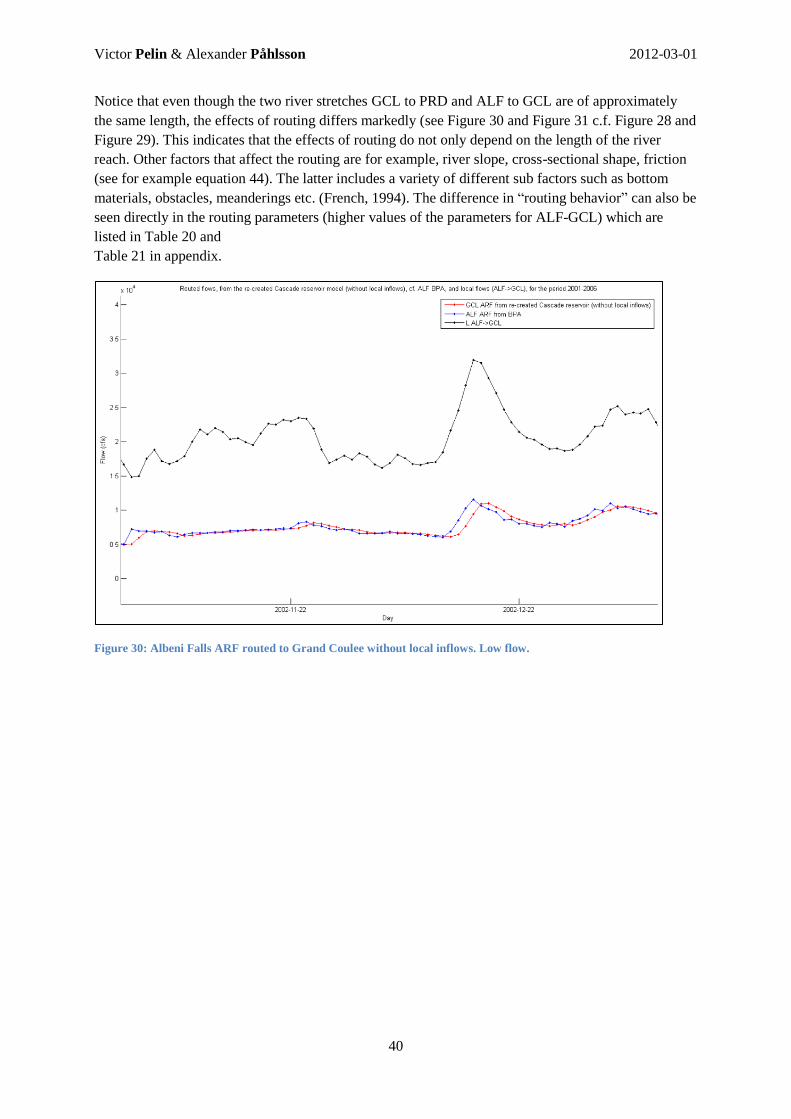
Victor Pelin & Alexander Påhlsson 2012-03-01
40
Notice that even though the two river stretches GCL to PRD and ALF to GCL are of approximately
the same length, the effects of routing differs markedly (see Figure 30 and Figure 31 c.f. Figure 28 and
Figure 29). This indicates that the effects of routing do not only depend on the length of the river
reach. Other factors that affect the routing are for example, river slope, cross-sectional shape, friction
(see for example equation 44). The latter includes a variety of different sub factors such as bottom
materials, obstacles, meanderings etc. (French, 1994). The difference in “routing behavior” can also be
seen directly in the routing parameters (higher values of the parameters for ALF-GCL) which are
listed in Table 20 and
Table 21 in appendix.
Figure 30: Albeni Falls ARF routed to Grand Coulee without local inflows. Low flow.

Victor Pelin & Alexander Påhlsson 2012-03-01
41
Figure 31: Albeni Falls ARF routed to Grand Coulee without local inflows. High flow.
4.3.3 Mica to The Dalles (distance 1300 km)
The stretch between Mica (MCD) and The Dalles (TDA) is shown on a map in Figure 12. In Figure 32
and Figure 33 below the effects of routing between MCD and TDA can be seen. Since MCD is at the
headwaters of Columbia River it is not unreasonable that the local inflows along the stretch are much
higher than the upstream inflow. Also there are many larger tributaries that connect to the main river
channel along this stretch, for example Snake River. The routing causes a time delay of about 2-3 days
(see Figure 32 and Figure 33). The differences in the effects of routing between high and low flows are
approximately one day in time delay. This clearly shows the flow dependence of the time of storage
and thereby the routing (see for example equation 35).
The attenuation is best seen in Figure 34. It can be seen that some peaks seem to be more dampened
than others (compare full and dashed circles in Figure 34). For the sake of reasoning, study equation
34, which is used in the cascade3 routing routine.
(
) (34)
It basically says that the flow at a certain time step is estimated by weighing the outflow and inflow at
a previous time step with the inflow at the current time step. This means that “sharp single peaks” will
be more dampened than peaks that persist over longer time. The fact that the shape of the hydrograph
largely affects the routing means that depending on which interpolation method the model uses, the
outflow hydrograph will be different. This supports the explanation that the errors in the model
verification likely are due to differences in interpolation methods between the cascade3 routing routine
and the routing routine in the SSARR model used by the BPA.

Victor Pelin & Alexander Påhlsson 2012-03-01
42
Figure 32: Mica ARF routed to The Dalles without local inflows. Low flow.
Figure 33: Mica ARF routed to The Dalles without local inflows. High flow.

Victor Pelin & Alexander Påhlsson 2012-03-01
43
Figure 34: Mica ARF routed to The Dalles without local inflows. A time period that displays visible effects of routing.
4.4 Applying the model in Columbia River – Lumped parameters
4.4.1 Lumping known parameter values
The procedure used in this chapter is described in chapter 3.3.2. Parameter values for all sub reaches
can be found in appendix Table 20. The sum of all phases from Mica (MCD) to The Dalles (TDA) is
(equation 50):
The total time of storage from MCD to TDA is:
The KTS parameter is (equation 52):
The n parameter is (equation 54):
4.4.2 Parameter values and resulting routing effects Mica to The Dalles
Figure 35 and Figure 36 show how well the lumped parameters (see Table 7) mimic the routing effects
from reach by reach routing. It is not a perfect fit (see Table 8) but it is a good starting point for
calibration, which will be done in chapter 4.7.

Victor Pelin & Alexander Påhlsson 2012-03-01
44
Table 7: Lumped parameter values, MCD-TDA.
Parameter Value
nbrPhases 43
n 0.2
KTS 8.65
Table 8: Objective functions for lumped parameter values, MCD-TDA.
Objective function Value
r2
0.997
Qav (cfs) 552
Figure 35: The effects of routing MCD-TDA. Lumped parameter approximation. High flow.

Victor Pelin & Alexander Påhlsson 2012-03-01
45
Figure 36: The effects of routing MCD-TDA. Lumped parameter approximation. Low flow.
4.5 Applying the model in the general case In the following section routing parameters are going to the approximated for the river reach Mica
(MCD) to The Dalles (TDA), in Columbia River, as they would have been approximated in the
general case when no parameter information is known a priori. This will be done with two different
methods, one that can be used when scarce amount of stream data is available and a second one when
some additional data is available.
4.5.1 Scarce amount of data
The n parameter
Equation 44 gives the following approximate value of n:
The assumptions that are included in this value are:
i. Uniform steady flow in the river channel
ii. Wide channel, which means that the width is much bigger than the depth (B>>y).
Although these assumptions in most cases may not be fulfilled, it can still serve as a first rough
estimation of the n parameter.
The number of phases parameter
If there is almost no data available for the river channel’s physical characteristics it is appropriate to
use equation 45, which is based on a suggestion from the U.S. Army Corps. Using this equation gives
the following number of phases:

Victor Pelin & Alexander Påhlsson 2012-03-01
46
Total time of storage
The total time of storage for a stream reach can be approximated to be equal to the time of travel for
the reach (USACE, 1991). The time of storage is estimated with equation 46 and the estimation
procedure is described more in detail in section 3.2.1.
The hydrograph at Grand Coulee (GCL) is plotted against the hydrograph at The Dalles (TDA)
(distance 620 km) in Figure 37. This was found to be an appropriate stream length, because the time
lag between peaks around the average flow was one day, which also was the time resolution of the
hydrograph data. The average flow between GCL and TDA is calculated by taking the mean of the
mean flow at each station. Figure 38 shows a zoomed view of the area inside of the dashed red circle
in Figure 37 with date marks at some of the peaks to show that the peak lag around the average flow in
this case is one day. The time of storage is then estimated according to equation 46:
An obvious problem with this method of estimating the total time of storage occurs when local inflows
are large in comparison to the upstream inflow. Then the figure, of the inflow and outflow hydrograph,
will not clearly show the lag time of the upstream flow because it will be disturbed by the shape of the
local inflow hydrograph. It is therefore important to study and compare hydrographs at different
geographical distances and over a long time period when applying this method.
Figure 37: Upstream and downstream hydrographs from the stations Grand Coulee (upstream) and The Dalles
(downstream).
0
50000
100000
150000
200000
250000
300000
350000
400000
450000
500000
2001-01-01 2001-03-12 2001-05-21 2001-07-30 2001-10-08 2001-12-17
Flo
w (
cfs)
Date (days)
Estimation of Ts
GCL
TDA
Average flow GCL->TDA
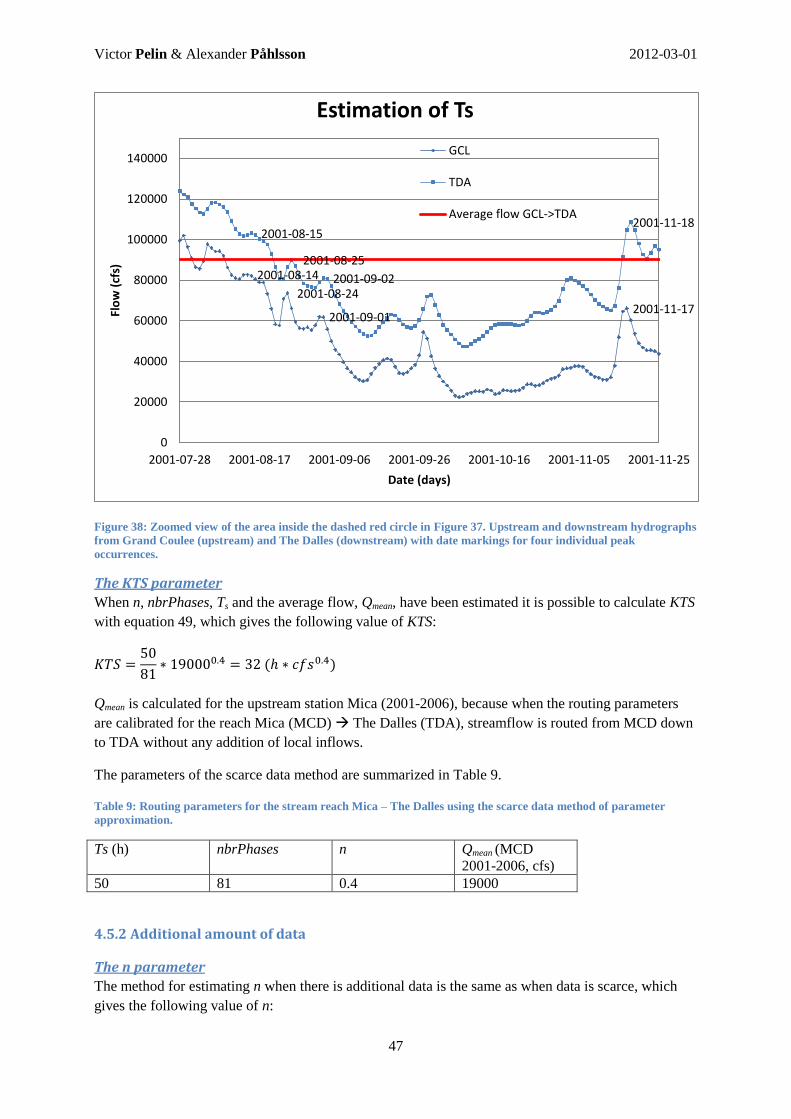
Victor Pelin & Alexander Påhlsson 2012-03-01
47
Figure 38: Zoomed view of the area inside the dashed red circle in Figure 37. Upstream and downstream hydrographs
from Grand Coulee (upstream) and The Dalles (downstream) with date markings for four individual peak
occurrences.
The KTS parameter
When n, nbrPhases, Ts and the average flow, Qmean, have been estimated it is possible to calculate KTS
with equation 49, which gives the following value of KTS:
Qmean is calculated for the upstream station Mica (2001-2006), because when the routing parameters
are calibrated for the reach Mica (MCD) The Dalles (TDA), streamflow is routed from MCD down
to TDA without any addition of local inflows.
The parameters of the scarce data method are summarized in Table 9.
Table 9: Routing parameters for the stream reach Mica – The Dalles using the scarce data method of parameter
approximation.
Ts (h) nbrPhases n Qmean (MCD
2001-2006, cfs)
50 81 0.4 19000
4.5.2 Additional amount of data
The n parameter
The method for estimating n when there is additional data is the same as when data is scarce, which
gives the following value of n:
2001-08-14
2001-08-24
2001-09-01 2001-11-17
2001-08-15
2001-09-02
2001-11-18
2001-08-25
0
20000
40000
60000
80000
100000
120000
140000
2001-07-28 2001-08-17 2001-09-06 2001-09-26 2001-10-16 2001-11-05 2001-11-25
Flo
w (
cfs)
Date (days)
Estimation of Ts
GCL
TDA
Average flow GCL->TDA

Victor Pelin & Alexander Påhlsson 2012-03-01
48
The nbrPhases parameter
Heatherman (2008) gives two methods for computing the nbrPhases parameter when additional data is
available (Table 10); equation 37 and equation 39. These two equations yield the following two values
of nbrPhases and the average of the two:
This approximation was made with data from the U.S. Geological Survey (USGS) at a station called
Vernita (USGS, n.d.), just downstream of Priest Rapids. The data in Table 10 was recorded on the 22nd
of May 1949 for the peak discharge, which in the approximation is used as the reference discharge. It
is obvious that using values of mean flow velocity, flow depth, top width and flow recorded at peak
discharge (and slope) at a point along a reach, does not give a value that is the most representative for
that particular reach. Furthermore the data is affected by the flow regulations from that time. But, it
gives a value that could be used as a reasonable starting point for calibration.
Table 10: Recorded data at Vernita, just downstream of Priest Rapids (USGS, n.d.).
Lreach S0 y0 v0 T Q0
4265000 ft 0.000194 30 ft 8.37 ft/s 1700 ft 406000 ft3/s
The total time of storage –Ts
When measurements of mean flow velocity are available, equation 48 can be used and Ts becomes:
In this particular case, where the mean velocity from Table 10 is used, the resulting value of Ts will
inherit the problems connected to the mean velocity, which was recorded at peak discharge and
perhaps not in a sub reach that is representative for the entire river. Thus, the time of storage estimated
using the scarce data method will in this case, when the additional data is of poor quality or relevance,
provide a better estimate than the additional data method. This is why a method that combines the
scarce and the additional data methods is presented in the next section.
The KTS parameter
Equation 49 gives the following value of KTS:
The parameters from the additional data method are summarized in Table 11.

Victor Pelin & Alexander Påhlsson 2012-03-01
49
Table 11: Routing parameters for the stream reach Mica – The Dalles using the additional data method of parameter
approximation.
KTS ( ) nbrPhases n Qmean (MCD
2001-2006, cfs)
99 49 0.4 19000
4.5.3 Combination scarce amount of data and additional data
As mentioned previously, the total time of storage parameter is in this case better estimated using the
scarce data method than the additional data method. However, for the nbrPhases parameter, using the
additional data method is possibly advantageous. A combination of the two methods yields the
following KTS value:
The parameters from the combined data method are summarized in Table 12.
Table 12: Routing parameters for the stream reach Mica – The Dalles using the combined method of parameter
approximation.
KTS ( ) nbrPhases n Qmean (MCD
2001-2006, cfs)
53 49 0.4 19000
4.5.4 Summary of parameter values and resulting routing effects Mica to The Dalles
Figure 39 to Figure 44 show how well the lumped model, with the general parameter approximations,
fit with the reach by reach routing. For high flows (see Figure 39 to Figure 41) the additional data
method appears to give the best fit. For low flows (see Figure 42 to Figure 44) the scarce and the
combined method appear to give the best fits. The time lag, the flow attenuation and the relation
between high and low flows are all slightly wrong, which suggests that all parameters need to be
adjusted by calibration. Since the lumped known parameters give the best fit this will be the starting
point in the sensitivity analysis (chapter 4.6) and the calibration (chapter 4.7).
According to the objective functions (see Table 14) the scarce and the combined methods give the best
general fit. However, in this case where are all the parameters for the sub reaches are known, the
lumped known parameter approximation gives the overall best fit. As can be seen in Table 13, the
nbrPhases parameter for the scarce amount of data method is somewhat larger than the rest. This is
likely because it is a very rough estimate that does not consider any properties of the catchment. The
KTS parameter is a direct result of the other parameters and the total time of storage (see equation 49)
and therefore also incorporates their variations.
Table 13: Summary of parameter values including the lumped parameters values from chapter 4.4, MCD-TDA.
Parameter Lumped known
parameters
Scarce amount of
data
Additional data Combination of
scarce and
additional data
nbrPhases 43 81 49 49
n 0.2 0.4 0.4 0.4
KTS ( ) 8.65 32 99 53

Victor Pelin & Alexander Påhlsson 2012-03-01
50
Table 14: Objective functions for lumped and general parameter approximations.
Parameter Lumped known
parameters
Scarce amount of data Additional data Combination of
scarce and additional
data
r2
0.99730 0.99022 0.98593 0.99038
Qav (cfs) 552 860 1400 846
Figure 39: The effects of routing MCD – TDA. General parameter approximation with scarce amount of data. High
flow.

Victor Pelin & Alexander Påhlsson 2012-03-01
51
Figure 40: The effects of routing MCD – TDA. General parameter approximation with additional amount of data.
High flow.
Figure 41: The effects of routing MCD – TDA. General parameter approximation with combined amount of data.
High flow.

Victor Pelin & Alexander Påhlsson 2012-03-01
52
Figure 42: The effects of routing MCD – TDA. General parameter approximation with scarce amount of data. Low
flow.
Figure 43: The effects of routing MCD – TDA. General parameter approximation with additional amount of data.
Low flow.

Victor Pelin & Alexander Påhlsson 2012-03-01
53
Figure 44: The effects of routing MCD – TDA. General parameter approximation with combined amount of data.
Low flow.
4.6 Sensitivity analysis The start values in this case are chosen to be the resulting values of the lumping of known parameters
(see chapter 4.4.1). These values give the best fit (see Table 14) compared to the reach-by-reach
routing and are therefore chosen as start values in the sensitivity analysis.
Figure 45: The result of the sensitivity analysis, Nash-Sutcliffe ratio.
0.88000
0.90000
0.92000
0.94000
0.96000
0.98000
1.00000
1.02000
-50% Start value +100%
Nas
h-S
utc
liffe
rat
io
Parameter change
Nash-Sutcliffe ratio
KTS
n
nbrPhases

Victor Pelin & Alexander Påhlsson 2012-03-01
54
Figure 46: The result of the sensitivity analysis, the average flow error.
The result of the sensitivity analysis is presented in Figure 45 and Figure 46. The lumped known
parameters are used as start values. Each parameter is then decreased by 50% and increased by 100%
and the resulting values of the objective functions are presented. The following remarks can be made:
The n parameter is the most sensitive parameter.
The KTS and nbrPhases parameters are almost equally sensitive.
The start values produce the best objective function results.
The fact that the n parameter is more sensitive to change than the other two is obvious since it
exponentially affects the total time of storage. The reason why KTS and nbrPhases are almost equally
sensitive is because they both linearly affect the total time of storage. They are not equally sensitive
because they affect attenuation differently. Notice that the start values produce the best results of the
objective functions. This means that to calibrate these parameters, changes smaller than the ones made
in the sensitivity analysis should be done.
The following steps are suggested when performing the calibration:
1. If the time lag is too large, decrease KTS, and vice versa, until the timing around the mean
flow is correct.
2. The “tilt” of timing between high and low flows can be altered using the n parameter. If high
flows have too large time lag, and low flows have too low time lag, increase n.
3. The attenuation is altered by changing nbrPhases and KTS simultaneously. To increase flow
attenuation without affecting the timing, the nbrPhases should be decreased and the KTS
increased by the same factor, and vice versa.
These three steps are repeated until the values of the objective functions and the resulting hydrograph
reach an acceptable result.
4.7 Calibrating the model To calibrate the model parameters for the entire Mica – The Dalles stretch, the lumped model
parameters from chapter 4.4 are used as start values. The calibration procedure used is the one
presented in chapter 4.6 above. Figure 47 and Figure 48 show an almost perfect fit, compared to the
0.00000
500.00000
1000.00000
1500.00000
2000.00000
2500.00000
3000.00000
3500.00000
-50% Start value +100%
Ave
rage
flo
w e
rro
r (c
fs)
Parameter change
Average flow error
KTS
n
nbrPhases

Victor Pelin & Alexander Påhlsson 2012-03-01
55
reach-by-reach routing, after calibration. The values of the objective functions in Table 16 show a
great improvement in the general fit as well.
The calibration procedure suggested in chapter 4.6 obviously works well. Mainly because it provides a
method with which one can manipulate individual routing effects. For example if, during calibration,
the timing around the mean flow is good, it is possible keep the total time of storage constant while
changing the attenuation (KTS and nbrPhases). This is possible since both the nbrPhases and KTS
parameter linearly affect the total time of storage (see for example equation 49).
Table 15: Parameter values before and after calibration.
Parameter Starting values Values after
calibration
nbrPhases 43 28
n 0.2 0.2
KTS (h*cfs0.2
) 8.65 15.8
Table 16: Values of the objective functions before and after the calibration.
Objective function Starting values Values after
calibration
r2
0.997 0.9999996
Qav (cfs) 552 6.17
Figure 47: The effects of routing MCD – TDA. Lumped parameter approximation after calibration. High flow.

Victor Pelin & Alexander Påhlsson 2012-03-01
56
Figure 48: The effects of routing MCD – TDA. Lumped parameter approximation after calibration. Low flow.
4.8 The importance of routing in hydrological models To get an idea of the importance of routing, three different cases (see Figure 14) with an increasing
level of routing of local inflows are presented below and compared with the full reach-by-reach routed
ARF flows from the cascade3 routing routine. This is further explained in the following sections.
4.8.1 No sub reaches
Figure 49 and Figure 50 show how well the flow hydrograph, if there is no routing of the local
inflows, fits the ARF data provided by the cascade3 routing routine. The timing of both high and low
flows is wrong; sometimes the time lag even differs by two days.

Victor Pelin & Alexander Påhlsson 2012-03-01
57
Figure 49: MCD routed to TDA, no routing of local inflows. Low flow.
Figure 50: MCD routed to TDA, no routing of local inflows. High flow.
4.8.2 Two sub reaches
In this case Columbia River is divided into two parts of roughly the same length, where the
accumulated local inflows for the first part is added in the middle (and then routed to the most
downstream station), while the accumulated local inflows for the second part is added at the most
downstream station. Figure 51 and Figure 52 show how well the flow hydrograph, when the division
of the stream described above is used, fits the ARF data provided by the cascade3 routing routine. The

Victor Pelin & Alexander Påhlsson 2012-03-01
58
timing and the attenuation of both high and low flows has clearly improved as compared to the case of
no routing of the local inflows.
Figure 51: MCD routed to TDA, two sub reaches with local inflows. Low flow.
Figure 52: MCD routed to TDA, two sub reaches with local inflows. High flow.
4.8.3 Four sub reaches
The division in this case is as in the preceding case with two sub reaches, but this time it is further
divided into four sub reaches. Figure 53 and Figure 54 show how well the flow hydrograph, when the
division of the stream described above is used, fits the ARF data provided by the cascade3 routing
routine. The timing and the attenuation of both high and low flows has further improved compared to
the previous case and the shape and timing of the hydrograph approaches the full reach-by-reach
hydrograph.

Victor Pelin & Alexander Påhlsson 2012-03-01
59
Figure 53: MCD routed to TDA, four sub reaches with local inflows. Low flow.
Figure 54: MCD routed to TDA, four sub reaches with local inflows. High flow.
4.8.4 Summary of the results of the objective functions
Table 17 shows a summary of the results above. The resulting values of the objective functions
improve as the number of divisions increase. Depending on what requirements of precision that the
full hydrological model has, the number of divisions can be decided upon accordingly. This decision
will be a compromise between simplicity and precision.
The crudest division (no sub reaches) gives a time delay of one or two days (see Figure 49 and Figure
50), which can be compared to the effects of routing (see Figure 32 and Figure 33) between Mica and
The Dalles that have a time delay of two to three days. This suggests that not only channel specific

Victor Pelin & Alexander Påhlsson 2012-03-01
60
properties (friction, slope, cross-sectional shape) affect the routing, but also the topology of the river,
i.e. how and where tributaries and local inflows are connected to the main river channel.
Table 17: Summary of the results of the objective functions.
Objective functions No sub reaches Two sub reaches Four sub reaches
r2
0.987 0.998 0.9993
Qav (cfs) 7530 2970 1760
4.9 Comparison with Muskingum routing The MATLAB code of the Muskingum routing routine is presented in appendix.
To calibrate the Muskingum model parameters for the entire stretch from Mica (MCD) to The Dalles
(TDA) (distance 1300 km), starting values are required for both K (h) and X (-). K is chosen as the
value of total time of storage (see Table 18), same as in chapter 4.4.1. The X parameter is chosen based
on Chow et al. (1988), who say that the mean value of X in natural streams is around 0.2.
Figure 55 and Figure 56 compare the routing effects of the calibrated Muskingum routing with the
cascade3 reach-by-reach routing. The figures show differences in routing effects between the two
methods, both in time lag and flow attenuation. Some peaks are more attenuated by the Muskingum
routing than the cascade3 routing, while other peaks are less attenuated. The lag time appears to be
better matched between the two models for high flows than for low flows. This difference in routing
between high and low flows is because the cascade3 routing is flow dependent, while the Muskingum
routing is not.
The values of the calibrated model parameters can be seen in Table 18. K does not change
significantly before and after the calibration, which indicates that the total time of storage is
approximately the same as travel time, K. Chow et al. (1988) and the U.S. Army Corps (1994) states
that the range of X is somewhere in between 0 and 0.5. Furthermore, Chow (1988) states that X for
natural streams usually is between 0 and 0.3. The calibrated value of X is 0.38, which is within
acceptable range of X according to the literature cited above.
Even though the two routing methods are different, they produce similar routing effects according to
the values of the objective functions in Table 19. Part of the reason why they are similar is that the
effects of routing are small. Furthermore, similarities between the methods can be seen in their
principles. If X in the Muskingum equation is set to zero then equation 18 reduces to the linear storage
equation 16. Additionally, if n is set to zero and the number of phases is set to one, then the cascade3
routing routine also reduces to the linear storage equation 16.
Table 18: Muskingum parameter values before and after calibration.
Parameter Start values Values after calibration
K (h) 51.2 63
X (-) 0.2 0.38
Table 19: Values of the objective functions before and after calibration.
Objective functions Start values Values after calibration
r2
0.991 0.994
Qav (cfs) 1040 819

Victor Pelin & Alexander Påhlsson 2012-03-01
61
Figure 55: The effects of routing, MCD – TDA, using both the cascade3 (reach-by-reach) routine and the Muskingum
method, high flow.
Figure 56: The effects of routing, MCD – TDA, using both the cascade3 (reach-by-reach) routine and the Muskingum
method, low flow.
4.10 Issues with the Bonneville Power Administration dataset The model verification for the shortest geographical distance (see chapter 4.2.1), which is Rock Island
(RIS) to Wanapum (WAN), was performed using the Bonneville Power Association (BPA)
streamflow data from 1984, as opposed to other stretches where the BPA data was taken from the

Victor Pelin & Alexander Påhlsson 2012-03-01
62
years 2001-2006. This was due to problems with the WAN ARF (Average daily unregulated Routed
Flow) from the last ten years. Figure 57 and Figure 58 shows the ARF data provided by BPA plotted
at RIS, WAN and Priest Rapids (PRD), which are three subsequent stations in Columbia River. The
figures also include the WAN ARF data provided by the cascade3 routing routine. Both figures show
that WAN has the highest flow, even though it is situated in between RIS and PRD and local inflows
between RIS and WAN is said to be negligible. The hydrograph at WAN is, over these years, in the
authors’ opinion, therefore unrealistic.
Figure 57: ARF data at RIS, WAN and PRD. High flow.
Figure 58: ARF data at RIS, WAN and PRD. Low flow.

Victor Pelin & Alexander Påhlsson 2012-03-01
63
Since the BPA dataset comprises 80 years of data from a large number of different dams and gaging
stations, it will inevitably contain data errors. In order to adjust these errors several different
techniques have been used by the BPA. Two major correction techniques are described and discussed
below.
A major problem with the data is that the dam storages (S) often are determined from elevation/storage
tables. The elevation is affected by for example wind setup, which induces severe errors in the storage
volumes. Since the dam inflows (A) are estimated using the outflow data (H) and the storage data (S)
according to equation 24, the errors in the storage volumes are also inherited in the dam inflows,
which sometimes causes negative inflows. To correct this, an arbitrary volume was added to the
storage on the affected day and then subtracted from another day the same month, in order to preserve
the overall monthly storage change volumes. This method is somewhat arbitrary and may not provide
a logical correction. Furthermore, even if the inflow values are positive they may still include errors
which were not adjusted for.
Another problem that concerns the local inflow data (L) is that it most of the time contains erratic
(irregular) spikes or negative values. To correct this, a method called indexing is used, which smooths
out the hydrograph so that it has a more reasonable hydrologic shape. Indexing involves calculating
the monthly average local inflow and the monthly average local flow at an adjacent index station. The
ratio of the local inflow average and the index average flow is then calculated. This ratio is then
multiplied with the daily index flows to get the hydrograph of the local inflow. As for the correction of
the storage volumes described in the previous section, the data is only corrected when there are
negative or irregular values. Even if the local inflows appear to be reasonable it could still contain
errors. Furthermore, the success of the indexing method depends on the quality of the adjacent station
data and also on how close the index station is.
Even if the correction methods are somewhat arbitrary, they still help to produce a reasonable dataset.
With such an extensive amount of data and the complexity of hydrology, it is a very difficult task to
handle.
4.11 Suggestions for further studies of the cascade3 routing routine To further evaluate the cascade3 routing routine and the importance of including routing in Thomson
Reuters Point Carbon’s proprietary hydrological HBV-type energy model, it is necessary to implement
the routing routine into the model and calibrate the routing routine and the model simultaneously. This
would give the ultimate answer to whether it is relevant to include streamflow routing in Thomson
Reuters Point Carbon’s proprietary hydrological HBV-type energy model.

Victor Pelin & Alexander Påhlsson 2012-03-01
64
5. Conclusion The Bonneville Power Administration (BPA) dataset is extensive and includes data from a great
number of stations throughout the Columbia River catchment (with an area larger than Sweden’s) over
80 years. The data has been revised and corrected repeatedly since 1970. Some of the correction
methods are somewhat arbitrary but produce reasonable data given the complex circumstances.
A routing routine (the cascade3 routing routine) based on the “cascade of reservoir” routing technique,
similar to the one used in the SSARR model, was developed. The routine was verified by using the
parameters and the average daily unregulated routed flow (ARF) data provided by the BPA. For short
distances (60 km) the routing routine gave very similar results to the routing in SSARR, whilst for
longer distances (1300 km) periods of poorer fit appeared. These are likely to be caused by the
differences in the interpolation methods between the routing routine in SSARR and the cascade3
routing routine.
A methodology for parameter estimation, in Columbia River and in the general case, was developed.
For the general case where the parameters are unknown, two alternative parameters estimation
methods were presented, one method that can be used with a scarce amount of data and a second one
for when additional data is available. Which of the methods that provides the best estimates largely
depends on the quality and appropriateness of the additional data.
The reasonableness of the routing produced by the cascade3 routing routine was evaluated using the
Muskingum method. The Muskingum method was calibrated to fit the effects of routing of the
cascade3 routing routine, and the calibrated Muskingum parameters were evaluated. The X parameter
was within reasonable range of the values for natural streams and the K parameter was close to the
total time of storage, which confirms the assumption that total time of storage is approximately the
same as the travel time.
The overall effects of routing in the Columbia River catchment are relatively small. The effects of
routing between Mica (MCD) and The Dalles (TDA) (distance 1300 km) are apparent with time lags
around 2-3 days and with noticeable flow attenuation. Most of the water in the Columbia River enters
as tributaries or local inflows along the flow path, which reduces the effects of routing at TDA. To get
a clear answer to whether it is favorable to include streamflow routing in a hydrological rainfall runoff
model, it is necessary to implement the routing routine into the model and calibrate them
simultaneously, which is suggested for future studies.

Victor Pelin & Alexander Påhlsson 2012-03-01
65
6. References Amenu, G.G., Killingtveit, Å., 2001. Real-time inflow forecasting for GilgelGibe reservoir, Ethiopia.
In: B. Honningsvåg, et al., ed. 2001. Hydropower in the New Millenium. Lisse: A.A.Balkema.
Bergström, S., 1976. Development And Application of a Conceptual Runoff Modell for Scandinavian
Catchments. Phd thesis. Lund: Institutionen för Teknisk Vattenresurslära, LTH, Lunds universitet.
Bonneville Power Administration United States Army Corps of Engineers, United States Bureau of
Reclamation, 2011. 2010 Level Modified Streamflow 1928-2008. Bonneville Power Administration,
Portland, OR.
Chadwick, A., Morfett, J., Borthwick, M., 2004. Hydraulics in civil and environmental engineering. 4th
ed. Abington: Spon Press.
Chaudhry, M.H., 2007. Open-Channel Flow. 2nd
ed. New York: Springer.
Chow, V.T., 1959. Open-Channel Hydraulics. New York: McGraw-Hill.
Chow, V. T., Maidment, D. R., Mays, L. W., 1988. Applied hydrology. New York: McGraw-Hill
Book Company.
French, R. H., 1994. Open-Channel Hydraulics. Singapore: McGraw-Hill Book Co.
Gordon, N.D., McMahon, T.A., Finlayson, B.L., Gippel, C.J., Nathan, R.J., 2004. Stream Hydrology –
An introduction for Ecologists. 2nd
ed. Chichester: John Wiley & Sons Ltd.
Google Earth, version 6.1.0.5001. (2011-10-17). Columbia River, 47°57'25.00"N, 118°58'50.93"W,
721. [Accessed 2011-12-22].
Hasan, E., Elshamy, M., 2011. Application of Hydrologial Models for Climate Sensitivity Estimation
of the Atbara Sub-basin. In: A.M. Melesse, ed. 2011. Nile Rive Basin – Hydrology, Climate and
Water Use. New York: Springer.
Heatherman, 2008. Flood Routing on Small Streams: A Review of Muskingum-Cunge, Cascading
Reservoirs, and Full Dynamic Solutions. University of Kansas.
Henderson, F. M., 1966. Open Channel Flow. New York: MacMillan Publishing CO., inc.
Lindström, G., Johansson, B., Persson, M., Gardelin, M., Bergström, S., 1997. Development and test
of the distributed HBV-96 hydrological model. Journal of Hydrology, 201(1997), pp. 272-288.
Nash, J.E., 1957. The form of the instantaneous unit hydrograph. International Association of Science
and Hydrology, 45(3) pp. 114-121.
Nash, J.E., Sutcliffe, J.V, 1970. River flow forecasting through conceptual models. Journal of
Hydrology 10(1970), pp. 282-290.
Perumal, M., 1992. The cause of negative initial outflow with the Muskingum method. Hydrological
Sicence, 37(4) pp. 391-401.
Rantz, S.E., 1982. Measurement and Computation of Streamflow: Volume 2. Computation of
Discharge. Geological Survey Water-Supply Paper 2175. Washington: United States Government
Printing Office.

Victor Pelin & Alexander Påhlsson 2012-03-01
66
Rice C. E., Larson C. L., 1972. Methods for routing hydrographs through open channels. WRRC,
Bulletin 51.
Singh, V.P., Frevert, D.K, 2005. Watershed Models [online], pp. 245-272. United States: CRC Press.
Available at:
http://www.dhigroup.com/upload/dhisoftwarearchive/papersanddocs/waterresources/MSHE_Book_Ch
apter/MIKE_SHE_Chp10_in_VPSinghDKFrevert.pdf [Accessed 2012-01-18]
SMHI, n.d.a HBV-modellen 1972.[online] (updated 2011-09-16) Available at:
http://www.smhi.se/kunskapsbanken/hbv-modellen-1.17857 [Accessed 2012-01-18]
SMHI, n.d.b The HBV model. [online] (updated 2006-05-03) Available at:
http://www.smhi.se/sgn0106/if/hydrologi/hbv.htm [Accessed 2011-11-25]
Strelkoff, T. 1980. Comparative analysis of flood routing methods (Research Document 24). U.S.
Army Corps of Engineers, Hydrologic Engineering Center, Davis, California.
Subramanya, E., 2008. Engineering hydrology. 3rd ed. New Dehli: Tata McGraw-Hill Publishing
Company Limited.
Tingsanchali T., 1986. Flood Simulation in the Tidal Delta of the Mekong River by the SSARR
Model. Water International, 11(3), pp. 117-126.
USACE, 1991. SSARR: Model Streamflow Synthesis and Reservoir Regulation Model. North Pacific
Division, US Army Corps of Engineers, Portland, OR. Available online at: http://www.nwd-
wc.usace.army.mil/report/ssarr.htm [Accessed 2011-11-25]
USACE, 1994. Engineering and Design: Flood-Runoff Analysis. US Army Corps of Engineers,
Washington DC. Ch. 9.
USACE, 2000. Hydrologic Modeling System HEC-HMS, Technical reference manual.
USACE, n.d.. [online] (updated 2003-11-21) Available at: http://www.nwd-
wc.usace.army.mil/report/colmap.htm [Accessed 2012-01-22]
U.S. Environmental Protection Agency, n.d. Columbia River Basin. [online] (updated 2012-01-18)
Available at: http://yosemite.epa.gov/r10/ecocomm.nsf/Columbia/Columbia
USGS, n.d.. Columbia River at Vernita, Wash. [online] (updated 2011-09-22) Available at:
http://il.water.usgs.gov/proj/nvalues/db_barnes/sites/12464500.shtml [Accessed 2012-01-12].
Ward, R.C., Robinson, M., 2000. Principles of Hydrology. London: McGraw-Hill Publishing
Company.

Victor Pelin & Alexander Påhlsson 2012-03-01
67
7. Appendix A. Routing specifics Table 20: The full stepwise routing from Mica to the Dalles. Based on BPA (2011).
Stretch Parameters
KTS n nbrPhases
MCD->RVC RVC_ARF=(MCD_ARF routed to
RVC)+RVC_L
5.0 0.2 3.0
RVC->ARD ARD_ARF=(RVC_ARF routed to
ARD)+ARD_L
10.0 0.2 2.0
ARD->MUC MUC_ARF=((ARD_ARF+BRD_ARF)
routed to MUC)+MUC_L
10.0 0.2 4.0
MUC->CIB CIB_ARF=(MUC_ARF routed to
CIB)+WAT_ARF+LLK_ARF
10.0 0.2 2.0
CIB->GCL GCL_ARF=(CIB_ARF routed to
GCL)+GCL_L
30.0 0.2 2.0
GCL->CHJ CHJ_ARF=(GCL_ARF routed to
CHJ)+CHJ_L
6.0 0.2 2.0
CHJ->WEL WEL_ARF=(CHJ_ARF routed to
WEL)+WEL_L
5.0 0.2 2.0
WEL->RRH RRH_ARF=(WEL_ARF routed to
RRH)+RRH_L+CHL_A
8.0 0.2 2.0
RRH->RIS RIS_ARF=(RRH_ARF routed to
RIS)+RIS_L
5.0 0.2 2.0
RIS->WAN WAN_ARF=(RIS routed to WAN) 7.0 0.2 2.0
WAN->PRD PRD_ARF=(WAN routed to PRD)+PRD_L 5.0 0.2 2.0
PRD /IHR->CP CP_ARF=(PRD routed to CP)+IHR_ARF 25.0 0.2 5.0
YAK->CP CP_ARF=CP_ARF+(YAK routed to CP) 6.3 0.1 2.0
CP->MCN MCN_ARF=(CP routed to MCN)+MCN_L 15.0 0.2 3.0
MCN->JDA JDA_ARF=(MCN routed to JDA)+JDA_L 5.0 0.2 5.0
JDA->TDA TDA_ARF=(JDA routed to TDA)+TDA_L 7.0 0.2 3.0
Table 21. The full stepwise routing from Albeni Falls to Grand Coulee.
Stretch Parameters
KTS n nbrPhases Total Ts
ALF->BOX BOX_ARF=(ALF_ARF routed to
BOX)+BOX_L
30 0.2 4.0 16.6
BOX->BDY BDY_ARF=(BOX_ARF routed to
BDY)+BDY_L
10 0.2 4.0 5.5
BDY->SEV SEV_ARF=BDY_ARF+SEV_L No routing in this reach
SEV->WAT WAT_ARF=SEV_ARF+WAT_S No routing in this reach
MUC->CIB
WAT->CIB
CIB_ARF=(MUC_ARF routed to
CIB)+WAT_ARF+LLK_ARF
10
0.2 2.0 2.8
CIB->GCL GCL_ARF=(CIB_ARF routed to
GCL)+GCL_L
30 0.2 2.0 6.8

Victor Pelin & Alexander Påhlsson 2012-03-01
68
8. Appendix B. MATLAB code
The MATLAB code of the cascade3 routing routine function [OMD Ihr]=cascade3(P,ID) %-------------------------------------------------------------------------- %SYFTE % Beräkna routat dagligt utflöde från en flodsträcka med givna % kalibreringsparametrar % %INPUT: % P=[KTS n nbrPhases t tIndata] Kalibrerade parametrar. % ID: Dagliga inflöden i kolonnmatris % %OUTPUT: % OMD: Dagliga routade utflöden i kolonnmatris, medel av de 24 % senast passerade timmarna. % % Ihr: Lösningsmatrisen med timdata. %-------------------------------------------------------------------------- %Senast modifierad: Alexander och Victor 2011-12-16. %Skriven av Victor Pelin & Alexander Påhlsson 2011-11-03. %--------------------------------------------------------------------------
%Kalibrerade parametrar och koefficienter från INPUT KTS=P(1,1); n=P(1,2); nbrPhases=P(1,3); t=P(1,4); tIndata=P(1,5);
%Definition av matriser %Resultatmatrisen: Inflöden respektive utflöden till alla reservoarer. Ih=zeros(length(ID)*round(tIndata/t),nbrPhases+1); ODM=zeros(length(ID),1); %Dagliga routade medelflöden.
%Tim-inflöde interpoleras som konstant värdet under den aktuella dagen r=0; %Räknaren nollställs for i=1:length(ID) for k=1:round(tIndata/t) r=r+1; Ih(r,1)=ID(i); end end
%Utflöde från respektive reservoar läggs i nya kolumner i Ih-matrisen och %fungerar som inflöde till nästa reservoar for i=1:nbrPhases %Inflödet (för timme 1) till reservoar 2/3/... gissas vara inflöde till %reservoar 1/2 (bara ett schablon-värde för att kunna börja räkna) Ih(1,i+1)=Ih(1,i); for k=1:length(Ih)-1 Im=(Ih(k,i)+Ih(k+1,i))/2; %Medelvärde på inflödet under timme k %Lös ut utflödet Q vid slutet av timmen -från reservoar 1- och sätt %in som inflöde till reservoar 2 under nästa tidssteg osv: Ih(k+1,i+1)=fzero(@(Q) (Ih(k,i+1)+t*(Im-Ih(k,i+1))/((KTS/((Ih... (k,i+1)+Q)/2)^n)+t/2)-Q),Im); end end

Victor Pelin & Alexander Påhlsson 2012-03-01
69
%Dagliga medelvärden av utflöde (ODM) beräknas som baklänges interpolering. r=0; %Räknaren nollställs. for i=1:length(ID) %Summera flödena under 24 h dela med 24. Medel gäller för kommande dag. for k=1:round(tIndata/t) r=r+1; ODM(i)=ODM(i)+Ih(r,nbrPhases+1)/round(tIndata/t); end end
OMD=ODM; %Slutligen läggs data i OUTPUT-matriserna. Ihr=Ih; end %--------------------------------C'est ca----------------------------------

Victor Pelin & Alexander Påhlsson 2012-03-01
70
The MATLAB code of the r2 routine function rsquare=rSquare(Dobs,Dmod) %-------------------------------------------------------------------------- %SYFTE % Beräkna R^2-värdet mellan observerad data och modellerad data % %INPUT: % Dobs: Observerad data (kolonnmatris) % Dmod: Modellerad data (kolonnmatris) % %OUTPUT: % rsquare: Värdet på R^2 %-------------------------------------------------------------------------- %Last modified: Victor Pelin 2011-11-04 %Skriven av Alexander Påhlsson och Victor Pelin 2011-11-04. %-------------------------------------------------------------------------- y_mean=0; for i=1:length(Dobs(:,1)) y_mean=y_mean+Dobs(i,1)/length(Dobs(:,1)); end
SS_tot=0; SS_err=0; for i=1:length(Dobs(:,1)) SS_tot=SS_tot+(Dobs(i,1)-y_mean)^2; SS_err=SS_err+(Dobs(i,1)-Dmod(i,1))^2; end
rsquare=1-SS_err/SS_tot; %--------------------------------C'est ca----------------------------------

Victor Pelin & Alexander Påhlsson 2012-03-01
71
The MATLAB code of the Qav routine function qav=qAverage(Dobs,Dmod) %-------------------------------------------------------------------------- %SYFTE % Beräkna medel för absolutbeloppen av skillnaderna mellan uppmätta och % simulerade flöden % %INPUT: % Dobs: Observerad data (kolonnmatris) % Dmod: Modellerad data (kolonnmatris) % %OUTPUT: % qav: Värdet qav %-------------------------------------------------------------------------- %Senast modifierad: Victor Pelin och Alexander Påhlsson 2011-12-08 %Skriven av Alexander Påhlsson och Victor Pelin 2011-12-08. %--------------------------------------------------------------------------
Q_av_abs=0;
for i=1:length(Dobs) Q_av_abs=Q_av_abs+abs(Dmod(i,1)-Dobs(i,1)); end
Q_av_abs=Q_av_abs/length(Dmod);
qav=Q_av_abs;
end
%---------------------------------C'est ca---------------------------------

Victor Pelin & Alexander Påhlsson 2012-03-01
72
The MATLAB code for a routing example clear '-------------------------------------------------------------------------' format long %Reading daily inflows at RIS
ID=xlsread('RIS5ARF_daily.xls','B20274:B20639'); %Reading daily outflows at WAN
OD=xlsread('WAN5ARF_daily.xls','B20274:B20639'); %Reading the date strings (for plotting)
[noll dates]=xlsread('WAN5ARF_daily.xls','A20274:A20639');
%Calibrated parameters (Appendix F: BPA, 2011)
KTS=7; n=0.2; nbrPhases=2; t=1; %Computational time step (hours) tIndata=24; %Time scale of input data (hours) P=[KTS n nbrPhases t tIndata];
[OMD Ihr]=cascade3(P,ID); %Time to route with cascade3
%Drawing graphs
figure(1) %Daily data hold on time=datenum(dates); plot(time,OD,'b.-') plot(time,OMD,'g.-') plot(time,ID,'k.-') set(gca,'XTick',724642:10:725007) datetick('x', 29, 'keepticks') xlabel('Day') ylabel('Flow (cfs)') title('Routed flows from cascade cf. to routed flows from BPA. 1984.') legend('ARF at WAN from BPA','ARF at WAN from cascade',... 'ARF at RIS (upstream) from BPA') hold off
figure(2) %Data at the computational time step scale hold on plot(Ihr(:,1),'b.-') plot(Ihr(:,nbrPhases+1),'r.-') xlabel('Computational time step') ylabel('Flow (cfs)') title('Routed flows at WAN from cascade cf. to inflow at RIS. 1984.'); legend('ARF at RIS, from BPA. Constant interpolation of inflow'... ,'ARF at WAN from cascade') hold off
%Controlling the computational time step Tmax=KTS./(max(Ihr)).^n; if Tmax<t/2 'Tidssteget t är för stort, prova ett mindre' else 'Tidssteget t är tillräckligt litet' end
%Objective functions: The R^2 value and the average deviation.
R2_WAN=rSquare(OD,OMD) qAv=qAverage(OD,OMD) '-------------------------------------------------------------------------'

Victor Pelin & Alexander Påhlsson 2012-03-01
73
The MATLAB code of the Muskingum routing routine function [OMD Ihr]=muskingum(P,ID) %-------------------------------------------------------------------------- %SYFTE % Beräkna routat dagligt utflöde från en flodsträcka med givna % kalibreringsparametrar % %INPUT: % P=[K X t tIndata] Kalibrerade parametrar. Tidssteget i timmar. % % ID: Dagliga inflöden i kolonnmatris % %OUTPUT: % OMD: Dagliga routade utflöden, medelvärden med tidsteget % tIndata. % % Ihr: Lösningsmatrisen med data i tidsteget t. %-------------------------------------------------------------------------- %Senast modifierad: Alexander och Victor 2012-01-30. %Skriven av Victor Pelin & Alexander Påhlsson 2012-01-30. %--------------------------------------------------------------------------
%Kalibrerade parametrar och koefficienter från INPUT K=P(1,1); X=P(1,2); t=P(1,3); tIndata=P(1,4);
%Definition av matriser %Resultatmatrisen: Inflöden respektive utflöden till alla reservoarer. Ih=zeros(length(ID)*round(tIndata/t),1); ODM=zeros(length(ID),1); %Dagliga routade medelflöden.
%Tim-inflöde interpoleras som konstant värdet under den aktuella dagen r=0; %Räknaren nollställs for i=1:length(ID) for k=1:round(tIndata/t) r=r+1; Ih(r,1)=ID(i); end end
%Utflöde från respektive reservoar läggs i nya kolumner i Ih-matrisen och %fungerar som inflöde till nästa reservoar
%Inflödet (för timme 1) till reservoar 2/3/... gissas vara inflöde till %reservoar 1/2 (bara ett schablon-värde för att kunna börja räkna) Ih(1,2)=Ih(1,1);
%Konstanterna C1, C2 och C3 beräknas från parametrarna. C1=(t-2*K*X)/(2*K*(1-X)+t); C2=(t+2*K*X)/(2*K*(1-X)+t); C3=(2*K*(1-X)-t)/(2*K*(1-X)+t);
%Lösningsrutinen: for k=1:length(Ih)-1 Ih(k+1,2)= C1*Ih(k+1,1)+C2*Ih(k,1)+C3*Ih(k,2); end

Victor Pelin & Alexander Påhlsson 2012-03-01
74
%Dagliga medelvärden av utflöde (ODM) beräknas som baklänges interpolering. r=0; %Räknaren nollställs. for i=1:length(ID) %Summera flödena under 24 h dela med 24. Medel gäller för kommande dag. for k=1:round(tIndata/t) r=r+1; ODM(i)=ODM(i)+Ih(r,2)/round(tIndata/t); end end
OMD=ODM; %Slutligen läggs data i OUTPUT-matriserna. Ihr=Ih; end %--------------------------------C'est ca-------------------------------