Graduate Theses and Dissertations Iowa State University Capstones, Theses andDissertations

2010

Evaluation of mechanistic-based compactionmeasurements for earthwork QC/QAJiake ZhangIowa State University

Follow this and additional works at: https://lib.dr.iastate.edu/etd

Part of the Civil and Environmental Engineering Commons

This Thesis is brought to you for free and open access by the Iowa State University Capstones, Theses and Dissertations at Iowa State University DigitalRepository. It has been accepted for inclusion in Graduate Theses and Dissertations by an authorized administrator of Iowa State University DigitalRepository. For more information, please contact digirep@iastate.edu.

Recommended CitationZhang, Jiake, "Evaluation of mechanistic-based compaction measurements for earthwork QC/QA" (2010). Graduate Theses andDissertations. 11547.https://lib.dr.iastate.edu/etd/11547

Evaluation of mechanistic-based compaction measurements for earthwork QC/QA

by

Jiake Zhang

A thesis submitted to the graduate faculty

in partial fulfillment of the requirements for the degree of

MASTER OF SCIENCE

Major: Civil Engineering (Geotechnical Engineering)

Program of Study Committee: David White, Major Professor

Vernon Schaefer Max Morris

Iowa State University

Ames, Iowa

2010

Copyright © Jiake Zhang, 2010. All rights reserved.

ii

TABLE OF CONTENTS

LIST OF FIGURES ....................................................................................................................... IV

LIST OF TABLES ........................................................................................................................ IX

LIST OF SYMBOLS ..................................................................................................................... X

ABSTRACT ................................................................................................................................. XII

CHAPTER 1. INTRODUCTION ................................................................................................... 1

Goals.................................................................................................................................... 2 Objectives ............................................................................................................................ 2 Significance ......................................................................................................................... 3 Thesis Organization............................................................................................................. 3

CHAPTER 2. BACKGROUND ..................................................................................................... 4

Light Weight Deflectometer (LWD) ................................................................................... 4 Size of LWD loading plate ...................................................................................... 4 Plate contact stress .................................................................................................. 6

Falling Weight Deflectometer (FWD) ................................................................................ 7 Plate Load Test (PLT) ......................................................................................................... 8 Briaud Compaction Device (BCD) ..................................................................................... 8 Dynamic Cone Penetrometer (DCP) ................................................................................. 10 Influence of Soil Layering................................................................................................. 13 Correlations between LWD and Other In Situ Point Measurements ................................ 13 Target Value Determination for Quality Assurance ......................................................... 14

Gyratory Compactor .............................................................................................. 14 Pressure Distribution Analyzer (PDA) .................................................................. 15

CHAPTER 3. TEST METHODS .................................................................................................. 17

Field Test Methods ............................................................................................................ 17 Laboratory Test Methods .................................................................................................. 23

Soil Index Properties Tests .................................................................................... 23 Laboratory Compaction Tests ............................................................................... 24 Laboratory Strength Tests ..................................................................................... 26

CHAPTER 4. MATERIALS ......................................................................................................... 29

TH 60 – Bigelow ............................................................................................................... 30 US 10 – Staples ................................................................................................................. 35

iii

Western Iowa loess............................................................................................................ 37 Geosynthetic Reinforcement Study ................................................................................... 39 Hormel PCC ...................................................................................................................... 43 Ohio Bridge Approach ...................................................................................................... 44 FHWA Intelligent Compaction (IC) ................................................................................. 46 Pavement Foundation Study.............................................................................................. 49

CHAPTER 5. TEST RESULTS AND DISCUSSION.................................................................. 52

Case Studies of Field Projects ........................................................................................... 52 Geosynthetic Reinforcement Study ....................................................................... 52 Hormel PCC .......................................................................................................... 57 Ohio Bridge Approach .......................................................................................... 68 FHWA Intelligent Compaction (IC) ..................................................................... 88 Pavement Foundation Study.................................................................................. 90

Influence of Device Configuration .................................................................................... 92 Correlations between LWD and Other in situ Point Measurements ................................. 97 Influence of Layered Soil Profiles on Surface Modulus ................................................. 101 Laboratory Test Results .................................................................................................. 104

Results from rigid boundary conditions .............................................................. 105 Results from flexible boundary conditions ......................................................... 109

Relationship between PDA Shear Resistance and Undrained Shear Strength ................ 114 Relationship between PDA Shear Resistance and Resilient Modulus ............................ 116 Establish Field Target Values for Quality Assurance ..................................................... 121 Linking Laboratory LWD-TVs to In situ LWD Measurements ..................................... 122

CHAPTER 6. CONCLUSIONS AND RECOMMENDATIONS .............................................. 129

REFERENCES ............................................................................................................................ 131

ACKNOWLEDGEMENTS ........................................................................................................ 135

APPENDIX I: FIELD TEST DATA ........................................................................................... 136

APPENDIX II: STATISTICAL MODELS ................................................................................ 161

iv

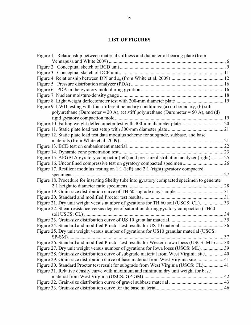
LIST OF FIGURES

Figure 1. Relationship between material stiffness and diameter of bearing plate (from Vennapusa and White 2009) ............................................................................................... 6

Figure 2. Conceptual sketch of BCD unit ...................................................................................... 9 Figure 3. Conceptual sketch of DCP unit ..................................................................................... 11 Figure 4. Relationship between DPI and su (from White et al. 2009) ........................................... 12 Figure 5. Pressure distribution analyzer (PDA) ........................................................................... 16 Figure 6. PDA in the gyratory mold during gyration ................................................................... 16 Figure 7. Nuclear moisture-density gauge .................................................................................... 18 Figure 8. Light weight deflectometer test with 200-mm diameter plate ....................................... 19 Figure 9. LWD testing with four different boundary conditions: (a) no boundary, (b) soft

polyurethane (Durometer = 20 A), (c) stiff polyurethane (Durometer = 50 A), and (d) rigid gyratory compaction mold ........................................................................................ 19

Figure 10. Falling weight deflectometer test with 300-mm diameter plate .................................. 20 Figure 11. Static plate load test setup with 300-mm diameter plate ............................................. 21 Figure 12. Static plate load test data modulus scheme for subgrade, subbase, and base

materials (from White et al. 2009) .................................................................................... 21 Figure 13. BCD test on embankment material .............................................................................. 22 Figure 14. Dynamic cone penetration test ..................................................................................... 23 Figure 15. AFGB1A gyratory compactor (left) and pressure distribution analyzer (right) .......... 25 Figure 16. Unconfined compressive test on gyratory compacted specimen ................................. 26 Figure 17. Resilient modulus testing on 1:1 (left) and 2:1 (right) gyratory compacted

specimens .......................................................................................................................... 27 Figure 18. Procedure for inserting Shelby tube into gyratory compacted specimen to generate

2:1 height to diameter ratio specimens .............................................................................. 28 Figure 19. Grain-size distribution curve of TH 60 sugrade clay sample ...................................... 31 Figure 20. Standard and modified Proctor test results .................................................................. 31 Figure 21. Dry unit weight versus number of gyrations for TH 60 soil (USCS: CL) ................... 33 Figure 22. Shear resistance versus degree of saturation during gyratory compaction (TH60

soil USCS: CL) ................................................................................................................. 34 Figure 23. Grain-size distribution curve of US 10 granular material............................................ 35 Figure 24. Standard and modified Proctor test results for US 10 material ................................... 36 Figure 25. Dry unit weight versus number of gyrations for US10 granular material (USCS:

SP-SM) .............................................................................................................................. 37 Figure 26. Standard and modified Proctor test results for Western Iowa loess (USCS: ML) ...... 38 Figure 27. Dry unit weight versus number of gyrations for Iowa loess (USCS: ML) .................. 39 Figure 28. Grain-size distribution curve of subgrade material from West Virginia site ............... 40 Figure 29. Grain-size distribution curve of base material from West Virginia site ...................... 41 Figure 30. Standard Proctor test result for subgrade from West Virginia (USCS: CL) ................ 41 Figure 31. Relative density curve with maximum and minimum dry unit weight for base

material from West Virginia (USCS: GP-GM) ................................................................. 42 Figure 32. Grain-size distribution curve of gravel subbase material ............................................ 43 Figure 33. Grain-size distribution curve for the base material ...................................................... 46

v

Figure 34. Grain-size distribution for the embankment material .................................................. 47 Figure 35. Standard Proctor test result for embankment material................................................. 47 Figure 36. Standard Proctor test result for aggregate base material .............................................. 48 Figure 37. Grain-size distribution curve for the untrimmed base material (TB1&3) ................... 49 Figure 38. Grain-size distribution curve for material from test bed #2......................................... 50 Figure 39. Standard Proctor test result for material from test bed #2 ........................................... 50 Figure 40. Relative density curve with maximum and minimum dry unit weight for material

from test bed #1 ................................................................................................................. 51 Figure 41. Test bed layout for West Virginia field study.............................................................. 53 Figure 42. Overview of the site ..................................................................................................... 54 Figure 43. Caterpillar (left) and Case (right) smooth drum rollers used in the West Virginia

site ..................................................................................................................................... 54 Figure 44. ELWD compaction curves for W-PP-GT and BX1200 sections .................................... 55 Figure 45. ELWD compaction curves for control and TX160 section ............................................ 56 Figure 46. Averaged ELWD compaction curves for each section ................................................... 57 Figure 47. Plan view of in situ test locations, results of crack survey using GPS and cracks on

the paved drive way (from White et al. 2009)................................................................... 58 Figure 48. FWD test results – paved drive way (from White et al. 2009) .................................... 59 Figure 49. LWD, CBR, and subbase thickness (interpreted from DCP-CBR profiles)

measurements on testing lane A (tests on unpaved area granular subbase) (from White et al. 2009) ......................................................................................................................... 60

Figure 50. LWD, CBR, and subbase thickness (interpreted from DCP-CBR profiles) measurements on testing lane B (tests on unpaved area granular subbase) (from White et al. 2009) ......................................................................................................................... 61

Figure 51. LWD, CBR, and subbase thickness (interpreted from DCP-CBR profiles) measurements on testing lane C (tests on unpaved area granular subbase) (from White et al. 2009) ......................................................................................................................... 62

Figure 52. LWD, CBR, and subbase thickness (interpreted from DCP-CBR profiles) measurements on testing lane D (tests on unpaved area granular subbase) (from White et al. 2009) ......................................................................................................................... 63

Figure 53. DCP-CBR profiles on testing lane A – unpaved area granular subbase (from White et al. 2009) .............................................................................................................. 64

Figure 54. DCP-CBR profiles on testing lane B – unpaved area granular subbase (from White et al. 2009) ......................................................................................................................... 65

Figure 55. DCP-CBR profiles on testing lane C – unpaved area granular subbase (from White et al. 2009) ......................................................................................................................... 66

Figure 56. DCP-CBR profiles on testing lane D – unpaved area granular subbase (from White et al. 2009) .............................................................................................................. 67

Figure 57. Bridge #1(BUT-75-0660) at I-75 &SR 129 interchange: (a) location of south and north MSE walls; (b) DCP test locations; (c) watering of backfill prior to compaction; (d) compaction of backfill next to the wall ....................................................................... 70

Figure 58. DCP-CBR profiles at location away from the NE and SW MSE walls – Bridge #1 ... 70 Figure 59. CBR at different depths from the top of the MSE wall at locations away from the

walls – Bridge #1............................................................................................................... 71 Figure 60. Moisture and dry density measurements at locations away from the MSE walls –

vi

Bridge #1 ........................................................................................................................... 71 Figure 61. Bridge #2 at Wilmington: (a) overview of the south MSE wall; (b) DCP test

locations; (c) vibratory plate compactor used to compaction of wall backfill .................. 73 Figure 62. DCP-CBR profiles at locations away from the MSE wall – Bridge #2 (USCS: SW-

SM) .................................................................................................................................... 74 Figure 63. Bridge #3 (MOT-75-1393) at downtown Dayton ........................................................ 75 Figure 64. DCP-CBR profiles at locations away from south wall and paving notch at east

abutment – Bridge #3 ........................................................................................................ 76 Figure 65. ELWD-Z2 measurements at locations away from paving notch and south wall on the

east abutment – Bridge #3 ................................................................................................. 76 Figure 66. Bridge #4 (FRA-670-0904B) near Columbus airport .................................................. 77 Figure 67. DCP-CBR profiles at locations away from the abutment – Bridge #4 ........................ 78 Figure 68. ELWD-Z2 at locations away from the approach slab – Bridge #4 ................................... 78 Figure 69. Bridge #5 (LIC-37-1225L) at Licking 161 over Moot Creek ...................................... 80 Figure 70. Proctor curve and field moisture and dry density measurement – Bridge #5 .............. 81 Figure 71. DCP-CBR profiles at locations away from the east and west abutments – Bridge

#5 ....................................................................................................................................... 81 Figure 72. ELWD-Z2 measurements at locations away from the east and west abutments –

Bridge #5 ........................................................................................................................... 82 Figure 73. Moisture and dry density measurements at locations away from the east and west

abutments – Bridge #5....................................................................................................... 82 Figure 74. Bridge #6 (MED-71-0729) at I-71 and I-76 interchange: (a) location of test site;

(b) void under the existing slab and old backfill material (c) in situ test locations – east lane (d) in situ test locations – west lane ................................................................... 84

Figure 75. DCP-CBR profiles at locations away from the south abutment for west and east lanes – Bridge #6 (USCS: GP-GM) .................................................................................. 85

Figure 76. ELWD-Z2 at locations away from the south abutment on east and west lanes – Bridge #6 ........................................................................................................................... 85

Figure 77. Stress-strain curves for static plate load tests – Bridge #6 .......................................... 86 Figure 78. Bridge #7 (MED-71-0750) at I-71 and I-76 interchange: (a) site location; (b) in

situ test locations ............................................................................................................... 87 Figure 79. DCP-CBR profiles at locations away from east abutment – Bridge #7 ....................... 87 Figure 80. ELWD-Z2 at locations away from east abutment – Bridge #7 ........................................ 88 Figure 81. Overview for test bed 1 ................................................................................................ 91 Figure 82. Overview for test bed 2 ................................................................................................ 92 Figure 83. Overview for test bed 3 ................................................................................................ 92 Figure 84. Correlations between ELWD with different sizes of loading plate ................................ 95 Figure 85. Relationship between ELWD and ELWD-Z2 with different bearing plate ......................... 96 Figure 86. Relationship between ELWD and ELWD-Z1.5 with different bearing plate ....................... 96 Figure 87. Correlations between ELWD and EFWD with 300 mm diameter loading plate ............... 99 Figure 88. Correlation between LWD measurement and BCD measurements............................. 99 Figure 89. Correlation between LWD measurements and PLT measurements for West

Virginia site ..................................................................................................................... 100 Figure 90. Correlation between ELWD-Z3 and PLT measurements for New York project site ..... 100 Figure 91. Correlation between ELWD-Z3 and PLT measurements for Michigan site .................. 101

vii

Figure 92. Sample calculation for estimating the equivalent modulus using DCP measurements .................................................................................................................. 102

Figure 93. Correlation between Eequivalent and ELWD-Z2 for Ohio project site ............................... 103 Figure 94. Correlation between Eequivalent and ELWD-Z2 for Hormel PCC project site .................. 103 Figure 95. Correlation between Eequivalent and ELWD-Z2 for West Virginia project site ................ 104 Figure 96. ELWD-Z1 contours in relationship with moisture and dry unit weight – US 10

granular material (USCS: SP-SM) (dLWD-Z1 = 85/ELWD-Z1) ............................................. 106 Figure 97. ELWD-Z1 contours in relationship with moisture and dry unit weight – TH36 silty

clay material (USCS: ML) (dLWD-Z1 = 59.4/ELWD-Z1) ...................................................... 106 Figure 98. ELWD-Z1 contours in relationship with moisture and dry unit weight – TH60 soil

301 material (USCS: CL) (dLWD-Z1 = 49.8/ELWD-Z1) ........................................................ 107 Figure 99. ELWD-Z1 contours in relationship with moisture and dry unit weight – TH60 (301,

303, and 305 combined) non-granular material (USCS: CL) (dLWD-Z1 = 49.8/ELWD-Z1) . 107 Figure 100. DPI contours in relationship with moisture and dry unit weight – TH60 non-

granular material (301, 303, and 305 combined) (USCS: CL) ....................................... 108 Figure 101. su contours in relationship with moisture and dry unit weight – TH60 non-

granular material (301, 303, and 305 combined) (USCS: CL) (su determined from empirical relationship with DPI) ..................................................................................... 108

Figure 102. Shear resistance versus number of gyrations (σo = 300 kPa) for TH 60 soil 306 (USCS: CL) ..................................................................................................................... 111

Figure 103. Shear resistance versus number of gyrations for US10 granular material (USCS: SP-SM) (σo = 300 kPa) .................................................................................................... 111

Figure 104. Influence of moisture content on τG for TH60 – soil 306 non-granular (USCS: CL) and US 10 granular (USCS: SP-SM) materials ....................................................... 112

Figure 105. Influence of boundary conditions on LWD measurements on gyratory compacted specimens at different moisture contents – TH 60 soil 306 (USCS: CL) ....................... 112

Figure 106. Relationships between LWD measurements and τG for different boundary conditions – TH 60 soil 306 (USCS: CL) ....................................................................... 113

Figure 107. Influence of boundary conditions on LWD measurements on gyratory compacted specimens at different moisture contents – US10 granular material (USCS: SP-SM) ... 113

Figure 108. Relationship between LWD measurements and τG for different boundary conditions – US10 granular material (USCS: SP-SM) ................................................... 114

Figure 109. τG versus number of gyrations for loess (USCS: ML) ............................................. 115 Figure 110. su and τG versus moisture content for gyratory compacted specimens after 100

gyrations at σo = 100, 300, and 600 kPa for loess (USCS: ML) .................................... 116 Figure 111. Relationship between su and τG for loess (USCS: ML) ........................................... 116 Figure 112. Effect of height to diameter ratio (H/D = 1 and 2) on Mr of gyratory compacted

specimens at σo = 100, 300 and 600 kPa at 100 gyrations –TH-60 soil 306 (USCS: CL) .................................................................................................................................. 119

Figure 113. Relationship between H/D = 2:1 and 1:1 Mr results on gyratory compacted specimens – TH60 soil 306 (USCS: CL) ........................................................................ 120

Figure 114. τG versus number of gyrations for σo = 100, 300, and 600 compacted specimens TH60 soil 306 (USCS: CL) ............................................................................................. 120

Figure 115. Correlation between su, Mr and τG for samples with H/D = 1 and 2 – TH 60 soil

viii

306 (USCS: CL) .............................................................................................................. 121 Figure 116. Results from in situ LWD tests showing ELWD increase and dLWD decrease with

number of blows at locations with different in situ moisture contents – TH60 .............. 122 Figure 117. ELWD-Z1 and ELWD-Z1.5 contours in relationship with moisture and dry unit weight

with stiff boundary conditions – TH60 soil 306 material (USCS: CL) .......................... 124 Figure 118. DPI and su contours in relationship with moisture and dry unit weight with stiff

boundary conditions – TH60 soil 306 material (USCS: CL) .......................................... 124 Figure 119. τG contours in relationship with moisture and dry unit weight with stiff boundary

test – TH60 soil 306 material (USCS: CL) ..................................................................... 125 Figure 120. Correlations between τG and LWD/DPI measurements with different boundary

conditions – TH60 soil 306 material (USCS: CL) (from White et al. 2009) .................. 126 Figure 121. Relationships between laboratory ELWD-Z1 and ELWD-Z2 measurements in

comparison with Terzaghi’s theoretical relationships – TH60 soil 306 material (USCS: CL) (from White et al. 2009) ............................................................................. 127

Figure 122. Comparison between in situ LWD measurements and laboratory predicted LWD target values (TH60 soil 306 “stiff” boundary model) (from White et al. 2009) ............ 127

Figure 123. Comparison between in situ LWD measurements and laboratory predicted LWD target values (TH60 soil 301, 302, 303 combined rigid boundary model) (from White et al. 2009) ....................................................................................................................... 128

Figure 124. DCP profiles for W-PP-GT and BX1200 sections .................................................. 137 Figure 125. DCP profiles for W-PP-GT and BX1200 sections – subbase layer 1 ...................... 138 Figure 126. DCP profiles for W-PP-GT and BX1200 section – subbase layer 2 ....................... 139 Figure 127. DCP profiles for W-PP-GT and BX1200 sections – final full depth test ................ 140 Figure 128. DCP profiles for control and TX160 sections ......................................................... 141 Figure 129. DCP profiles for control and TX160 sections – subbase layer 1 ............................. 142 Figure 130. DCP profiles for control and TX160 sections – subbase layer 2 ............................. 143 Figure 131. DCP profiles for control and TX160 sections – final full depth test ....................... 144 Figure 132. CBR profiles for subgrade layer for W-PP-GT and BX1200 sections .................... 145 Figure 133. CBR profiles for subgrade layer for control and TX160 sections ........................... 145 Figure 134. CBR profiles for W-PP-GT and BX1200 sections – subbase layer 1 ..................... 146 Figure 135. CBR profiles for W-PP-GT and BX1200 sections – subbase layer 2 ..................... 146 Figure 136. CBR profiles for W-PP-GT and BX1200 sections – final full depth test ................ 147 Figure 137. CBR profiles for control and TX160 sections – subbase layer 1 ............................ 147 Figure 138. CBR profiles for control and TX160 sections – subbase layer 2 ............................ 148 Figure 139. CBR profiles for control and TX160 sections – final full depth test ....................... 148

ix

LIST OF TABLES

Table 1. Summary of devices utilized in this research .................................................................. 17 Table 2. Summary of investigated materials ................................................................................. 29 Table 3. Summary of the material properties for TH 60 non-granular soil .................................. 32 Table 4. Summary of the material properties for US 10 granular material ................................... 36 Table 5. Summary of the material properties for Western Iowa loess .......................................... 38 Table 6. Summary of the material index properties for West Virginia site .................................. 42 Table 7. Summary of the material properties for the gravel subbase material.............................. 43 Table 8. Summary of soil index properties for backfill materials (sampled by ODOT) ............... 44 Table 9. Summary of soil index properties for backfill materials (sampled by ISU) ................... 45 Table 10. Summary of material index properties from New York project site ............................. 48 Table 11. Summary of soil index properties for the tested materials ............................................ 51 Table 12. Summary of in situ testing at different bridge locations ............................................... 68 Table 13. Summary of test beds and performed in situ testing ..................................................... 89 Table 14. Field LWD measurements from FHWA New York site ............................................... 90 Table 15. Summary of measured ELWD with different sizes of loading plates .............................. 94 Table 16. Summary of relationships between ELWD and other in situ point measurements .......... 98 Table 17. Summary of laboratory determined w-γd-DPI/su/ELWD relationships ......................... 109 Table 18. Comparison of Mr for 2:1 and 1:1 height to diameter ratio specimens – TH-60 soil

306 (USCS: CL) .............................................................................................................. 118 Table 19. Summary of DCP testing on subgrade ........................................................................ 149 Table 20. Summary of DCP testing on subbase 1 ....................................................................... 150 Table 21. Summary of DCP testing on TB-A after trafficking subbase 2 .................................. 151 Table 22. Summary of DCP testing on TB-B after trafficking subbase 2 .................................. 152 Table 23. Raw data for the correlation between Eequivalent and ELWD-Z2 – Ohio Site .................... 153 Table 24. Raw data for the correlation between Eequivalent and ELWD-Z2 – Dubuque Site ............. 154 Table 25. Raw data for the correlation between Eequivalent and ELWD-Z2 – West Virginia ............ 156

x

LIST OF SYMBOLS

Symbol Description Units

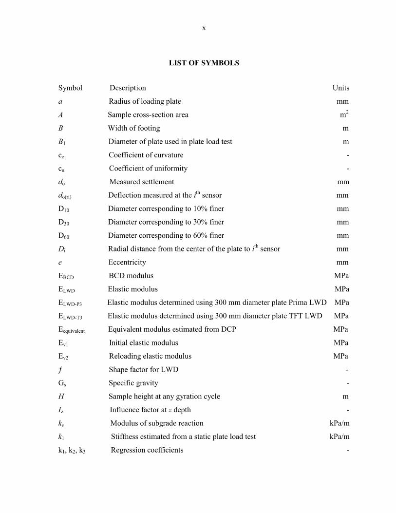
a Radius of loading plate mm

A Sample cross-section area m2

B Width of footing m

B1 Diameter of plate used in plate load test m

cc Coefficient of curvature -

cu Coefficient of uniformity -

do Measured settlement mm

do(ri) Deflection measured at the ith sensor mm

D10 Diameter corresponding to 10% finer mm

D30 Diameter corresponding to 30% finer mm

D60 Diameter corresponding to 60% finer mm

Di Radial distance from the center of the plate to ith sensor mm

e Eccentricity mm

EBCD BCD modulus MPa

ELWD Elastic modulus MPa

ELWD-P3 Elastic modulus determined using 300 mm diameter plate Prima LWD MPa

ELWD-T3 Elastic modulus determined using 300 mm diameter plate TFT LWD MPa

Eequivalent Equivalent modulus estimated from DCP MPa

Ev1 Initial elastic modulus MPa

Ev2 Reloading elastic modulus MPa

ƒ Shape factor for LWD -

Gs Specific gravity -

H Sample height at any gyration cycle m

Iz Influence factor at z depth -

ks Modulus of subgrade reaction kPa/m

k1 Stiffness estimated from a static plate load test kPa/m

k1, k2, k3 Regression coefficients -

xi

Symbol Description Units

Mr Resilient modulus MPa

P Applied load at surface N

Pa Atmospheric pressure MPa

R Resultant force N

z Depth from the surface mm

τG Shear resistance from gyratory compactor PDA kPa

θ Sum of principle stress or bulk stress MPa

σd Deviator stress MPa

ν Poisson’s ratio -

σo Applied stress MPa

r Radius of loading plate mm

ε Hoop strain on BCD plate -

γdmax Maximum dry unit weight kN/m3

wopt Optimum moisture content %

su Undrained shear strength kPa

σz Stress at depth of z kPa

xii

ABSTRACT

Compaction control for subgrade and base materials used in highway construction is

typically based on field tests in comparison to laboratory Proctor tests that determine the

relationship between dry unit weight and moisture content. The “optimum” moisture content

and maximum dry unit weight are established and then a minimum relative compaction value

and moisture content range is specified for acceptance during construction. This approach,

although widely accepted, does not directly determine the mechanistic properties of the

compacted material (i.e., strength or stiffness). The premise for adopting QA/QC tests that

determine mechanistic properties is that the QA/QC operations would more directly relate to

the design and also provide perhaps more value for ensuring quality as a final product. A

further limitation of standard QA/QC practices is that generally not enough information is

collected due to limited test frequency to ensure adequate reliability in quality over large

areas. Non-homogeneous vertical soil profiles are one aspect of in-situ testing that has largely

been ignored.

This study addressed these problems by evaluating five mechanistic-based devices in the

field and in the laboratory. Field studies were conducted at sites in West Virginia, Iowa,

Ohio, New York, and Michigan, to investigate the performance of five mechanistic-based

compaction control measurement devices. Laboratory tests were also performed to evaluate

relationship between moisture content, density, shear strength, and elastic/resilient modulus.

A unique aspect of this research in addition to the field studies is that gyratory compaction

samples were used to assess engineering properties of several soils and provided information

on moisture content, density, and shear resistance relationships during the compaction

process and a sample to test using other methods. Based on the comparison of the five

mechanistic-based devices conducted for this study, trends were observed between devices

and tradition density measurements, and the results provide data to evaluate the in situ

variability of compacted materials. The results of the laboratory study showed that gyratory

compacted samples provide useful information to determine mechanistic-based target values

for QC/QA practices.

1

CHAPTER 1. INTRODUCTION

The traditional approach for evaluating compaction quality of earth materials consists of

determining the moisture content (w) and dry unit weight (γd). Quality control (QC)

specifications typically require that the w and γd be within certain limits, and quality

assurance (QA) specifications require that w and γd be above some minimum value.

However, the w and γd are only surrogates to mechanistic properties which are used in

design. Design parameter values for pavements, slopes, foundations retaining structures, etc.

typically rely on strength or modulus/compressibility parameters. The study described here

focused on evaluating measurement technologies that link w and γd to mechanistic-based

parameters both in the laboratory and in the field.

Five mechanistic stiffness/strength measurement devices were evaluated in this study: light

weight deflectometer (LWD), falling weight deflectometer (FWD), plate load test (PLT),

Briaud compaction device (BCD), and dynamic cone penetrometer (DCP). The LWD and

FWD are dynamic tests, PLT is a static test, BCD is a small-strain test, and DCP is an

intrusive test. FWD and PLT have limitations that prevent wide spread implementation. For

example, the FWD needs a tow truck, which creates accessibility issues for the site, and PLT

needs a heavy load truck or frame to jack against. To make use of these devices, it is

important to have a better understanding for how these devices are related to each other, what

the factors that affect the measurements are and how target quality assurance values can be

developed. Further, variation in elastic modulus with depth surely affects the surface

measurement, but the impact of such condition has not been incorporated into practice.

To address these issues, both laboratory and field studies were covered in this research. A

series of LWD tests were performed in the field with different sizes of loading plates and

drop heights at the same applied stress to investigate the relationships between ELWD

measurements. Further, different in situ stiffness/strength measurement devices were applied

in the field to investigate their correlations for different field conditions. The correlation

study between DCP measurements and LWD measurements was conducted to evaluate the

2

influence of different layered soil conditions on the surface modulus. Based on the findings, a

standard protocol for developing ELWD target values is discussed in this research.

Multiple regression analysis was applied during the target value determination study.

Relationships between w, γd and ELWD were developed based on LWD measurements

performed on laboratory gyratory compacted samples. Statistical significance of each

variable was assessed based on p- and t- values.

Goals

The ultimate goals of this research were to investigate relationships between different in situ

stiffness/strength measurement devices (e.g., LWD, FWD, PLT, BCD, and DCP), to improve

the understanding of factors that affect the device measurements. Although several devices

were studied, the primary effort focused on LWD measurements.

Objectives

To effectively implement use of mechanistic in situ measurement devices for compaction

control and to establish target values for QC/QA, the following research objectives were

established for this study:

• obtain LWD measurements with different device configurations (i.e., diameter of

plate and surface contact stresses),

• correlate the LWD measurements with other in situ stiffness/strength measurements

(e.g., FWD, PLT, and BCD),

• investigate the effects of layered soil profiles on surface measurements,

• evaluate the relationship between ELWD, w and γd for gyratory compacted specimens

under rigid and flexible boundary conditions,

• link LWD laboratory measurements to field measurements and establish LWD target

values.

3

Significance

The results of this research will demonstrate the relationships between different in situ

stiffness/strength measurement devices and accelerate the implementation of these devices in

field compaction control. Further, the results from this research will document factors that

affect ELWD measurements and apply this new information to field practice for choosing

selecting suitable LWD configuration for compaction control. At last, a standard protocol for

ELWD target value determination for quality assurance was developed using gyratory

laboratory compacted specimens. The advantage of laboratory determination of target values

is that this work can be done prior to construction.

Thesis Organization

In addition to this introductory chapter, Chapter 2 discusses previous research that

investigated the factors that affect the ELWD measurement and reviews the literature of some

commonly used mechanistic-based compaction control devices. Chapter 3 describes the

laboratory and field test methods, and Chapter 4 summarizes the index properties of the

materials involved in this research. Chapter 5 presents field case studies of each of the six

test sites, provides tests results, and discusses these results as they relate to the study’s

objectives. The last chapter summarizes the conclusions from this research and offers

suggestions for future research.

4

CHAPTER 2. BACKGROUND

This chapter reviews previous studies of some commonly used in situ mechanistic-based

compaction control measurement devices. Seven soil compaction measurement devices were

involved in this study, a light weight deflectometer (LWD), a falling weight deflectometer

(FWD), a plate load test (PLT), a Briaud compaction device (BCD), a dynamic cone

penetrometer (DCP), and a gyratory compactor with pressure distribution analyzer (PDA).

Light Weight Deflectometer (LWD)

The LWD was developed to rapidly determine the in situ elastic modulus (ELWD) of

compacted fill materials. LWDs typically consist of a 100- to 300-mm diameter loading plate

with a drop weight of 10 kg; an accelerometer or geophones determine deflection; and a load

cell or calibration factor. In the field, the height of the drop weight is calibrated to determine

plate contact stress. The elastic modulus of the tested material can be determined by using the

deflection reading and the impact load of the drop weight.

The LWD measurements are affect by several factors, such as type and location of deflection

transducer, plate rigidity, loading rate, buffer stiffness, and measurement of load versus

assumption of load based on laboratory calibration from a standardized drop height, but this

study focused on two major factors, the size of the loading plate, and plate contact stress.

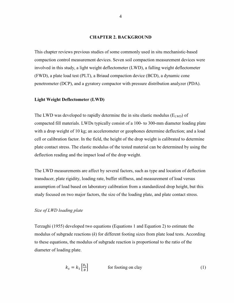
Size of LWD loading plate

Terzaghi (1955) developed two equations (Equations 1 and Equation 2) to estimate the

modulus of subgrade reactions (k) for different footing sizes from plate load tests. According

to these equations, the modulus of subgrade reaction is proportional to the ratio of the

diameter of loading plate.

�� � �� ���� � for footing on clay (1)

5

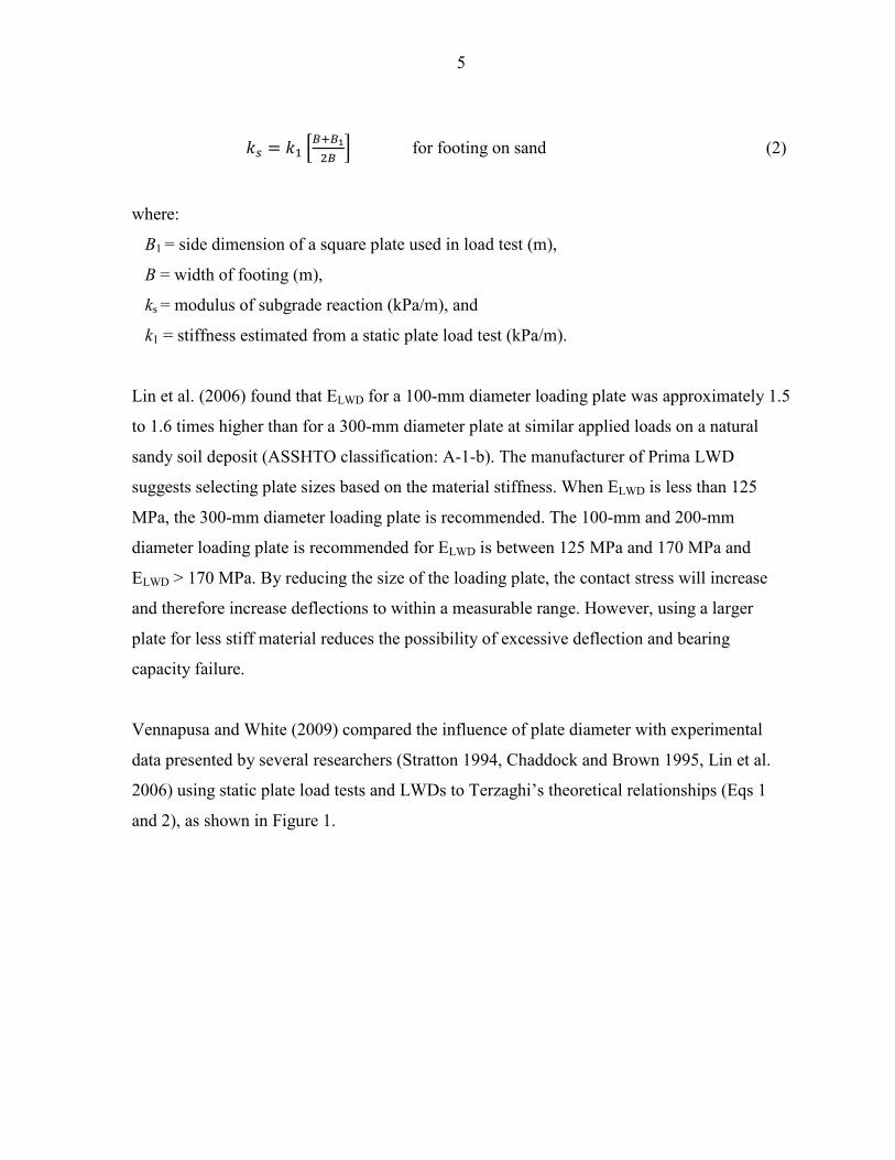
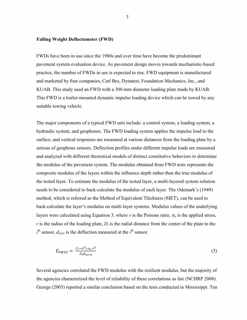
�� � �� ����� � for footing on sand (2)

where:

B1 = side dimension of a square plate used in load test (m),

B = width of footing (m),

ks = modulus of subgrade reaction (kPa/m), and

k1 = stiffness estimated from a static plate load test (kPa/m).

Lin et al. (2006) found that ELWD for a 100-mm diameter loading plate was approximately 1.5

to 1.6 times higher than for a 300-mm diameter plate at similar applied loads on a natural

sandy soil deposit (ASSHTO classification: A-1-b). The manufacturer of Prima LWD

suggests selecting plate sizes based on the material stiffness. When ELWD is less than 125

MPa, the 300-mm diameter loading plate is recommended. The 100-mm and 200-mm

diameter loading plate is recommended for ELWD is between 125 MPa and 170 MPa and

ELWD > 170 MPa. By reducing the size of the loading plate, the contact stress will increase

and therefore increase deflections to within a measurable range. However, using a larger

plate for less stiff material reduces the possibility of excessive deflection and bearing

capacity failure.

Vennapusa and White (2009) compared the influence of plate diameter with experimental

data presented by several researchers (Stratton 1994, Chaddock and Brown 1995, Lin et al.

2006) using static plate load tests and LWDs to Terzaghi’s theoretical relationships (Eqs 1

and 2), as shown in Figure 1.

6

Figure 1. Relationship between material stiffness and diameter of bearing plate (from Vennapusa and White 2009)

Plate contact stress

Previous research indicates that the measured deflection will increase with higher applied

contact stress. For example, Fleming et al. (2000) found that by increasing plate contact

stress from 35 kPa to 120 kPa the measured ELWD-P3 increased by 1.15 times, while ELWD-T3

increased by 1.3 times. Van Gurp et al. (2000) did similar research on very stiff crushed

aggregate and stabilized aggregate material, and for plate contact stress that varied from 140

kPa to 200 kPa no significant difference (< 3%) was observed.

Vennapusa and White (2009) conclude that for dense and compacted granular materials,

ELWD values tend to increase as the applied contact stress increase, except where the values

are influenced by underlying softer subgrade materials. For cementitious materials, the

measured ELWD was not sensitive to changes in contact stress.

Percentage of ks/k300 or Es/E300 or ELWD/ELWD-300

0 50 100 150 200 250 300 350

Diameter of P

late (mm)

50

100

150

200

250

300

350

400

450

500

550

Public Roads Testing - PLT (Stratton 1944)1

Omaha Testing - PL T (Stratton 1944)1

US Corps Testing - PLT (Stratton 1944)1

Crushed rock - LWD (Chaddock and Brown 1995)Sand - LWD (Lin et al. 2006)Field Study 3c - LWD2 Field Study 2 - LWD3 Eq 2 - PLT (Terzaghi and Peck 1967)Eq 3 - PLT (Terzaghi and Peck 1967)

1 Tests on subgrade soils2 Based on average of F ~ 2.7 to 7.5 kN3 Based on constant F = 7.07 kN for 300 mm plate and F = 6.7 kN for 200 mm plate

7

Falling Weight Deflectometer (FWD)

FWDs have been in use since the 1980s and over time have become the predominant

pavement system evaluation device. As pavement design moves towards mechanistic-based

practice, the number of FWDs in use is expected to rise. FWD equipment is manufactured

and marketed by four companies, Carl Bro, Dynatest, Foundation Mechanics, Inc., and

KUAB. This study used an FWD with a 300-mm diameter loading plate made by KUAB.

This FWD is a trailer-mounted dynamic impulse loading device which can be towed by any

suitable towing vehicle.

The major components of a typical FWD unit include: a control system, a loading system, a

hydraulic system, and geophones. The FWD loading system applies the impulse load to the

surface, and vertical responses are measured at various distances from the loading plate by a

serious of geophone sensors. Deflection profiles under different impulse loads are measured

and analyzed with different theoretical models of distinct constitutive behaviors to determine

the modulus of the pavement system. The modulus obtained from FWD tests represents the

composite modulus of the layers within the influence depth rather than the true modulus of

the tested layer. To estimate the modulus of the tested layer, a multi-layered system solution

needs to be considered to back-calculate the modulus of each layer. The Odemark’s (1949)

method, which is referred as the Method of Equivalent Thickness (MET), can be used to

back-calculate the layer’s modulus on multi-layer systems. Modulus values of the underlying

layers were calculated using Equation 3, where v is the Poisons ratio, σo is the applied stress,

r is the radius of the loading plate, Di is the radial distance from the center of the plate to the

ith sensor, do(ri) is the deflection measured at the ith sensor.

�� �� �� ������⋅σ�⋅���������� (3)

Several agencies correlated the FWD modulus with the resilient modulus, but the majority of

the agencies characterized the level of reliability of these correlations as fair (NCHRP 2008).

George (2003) reported a similar conclusion based on the tests conducted in Mississippi. Ten

8

subgrade test sections were built and evaluated with both in situ FWD test and laboratory Mr

test, and the correlation was not robust enough nor could be justified on a theoretical basis.

Plate Load Test (PLT)

PLT is a common in situ method for estimating modulus of subgrade reaction and soil

bearing capacity that has been used for many years. The major components of a typical plate

load test device are a 300 mm diameter rigid bearing plate, a 90-kN load cell, and three 50

mm linear voltage displacement transducers (LVDTs). PLT is conducted by loading the

bearing plate which is in contact with the surface and measuring the corresponding

deflections under load increments. The load is usually transmitted to the plate by a hydraulic

jack acting against heavy mobile equipment or a frame. The corresponding deflection is

measured by LVDTs which are arranged in triangle shape above the bearing plate and the

average of three readings are used in the calculation.

A typical PLT consists of initial and reload procedures, and the load and deformation

readings are continuously recorded during the test. The major drawbacks of PLTs are that

they are relatively slow, and they need a loaded truck or a frame, which introduces

accessibility issues for some project sites. In those cases, small-scale stiffness/strength

measurement devices, such as LWD, BCD are considered as the better options.

Briaud Compaction Device (BCD)

The BCD is a simple, small-strain, nondestructive testing apparatus for evaluating the

modulus of compacted soils, and it can be applied both in the laboratory and in the field as a

quality control testing tool (Weidinger and Ge 2009). BCD measurements are taken by

loading a thin, steel plate in contact with the compacted material and measuring the bending

strain of the plate, then relating that strain to the modulus of the compacted material. The

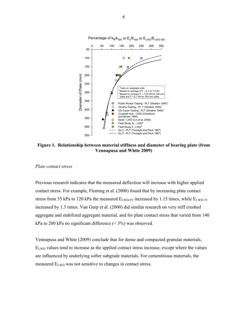
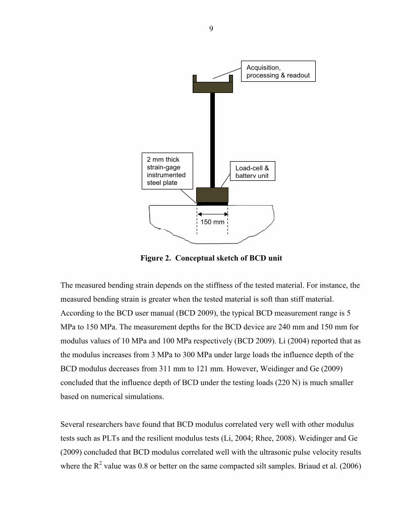
main components of the BCD are the acquisition processing and readout display unit, a load

cell, and a 2 mm thick strain-gage instrumented steel plate as shown in Figure 2.

9

Figure 2. Conceptual sketch of BCD unit

The measured bending strain depends on the stiffness of the tested material. For instance, the

measured bending strain is greater when the tested material is soft than stiff material.

According to the BCD user manual (BCD 2009), the typical BCD measurement range is 5

MPa to 150 MPa. The measurement depths for the BCD device are 240 mm and 150 mm for

modulus values of 10 MPa and 100 MPa respectively (BCD 2009). Li (2004) reported that as

the modulus increases from 3 MPa to 300 MPa under large loads the influence depth of the

BCD modulus decreases from 311 mm to 121 mm. However, Weidinger and Ge (2009)

concluded that the influence depth of BCD under the testing loads (220 N) is much smaller

based on numerical simulations.

Several researchers have found that BCD modulus correlated very well with other modulus

tests such as PLTs and the resilient modulus tests (Li, 2004; Rhee, 2008). Weidinger and Ge

(2009) concluded that BCD modulus correlated well with the ultrasonic pulse velocity results

where the R2 value was 0.8 or better on the same compacted silt samples. Briaud et al. (2006)

Acquisition, processing & readout

Load-cell & battery unit

2 mm thick strain-gage instrumented steel plate

150 mm

10

recommended a compaction control procedure that to perform BCD tests on the Proctor test

specimens confined in the mold in order to obtain the maximum BCD modulus and the

optimum water content for the material, which can be used to specify a percentage of the

maximum BCD modulus as the target value in the field.

Dynamic Cone Penetrometer (DCP)

DCPs are low cost, in situ strength measurement devices that are increasingly being

considered in geotechnical and foundation engineering for site investigation and quality

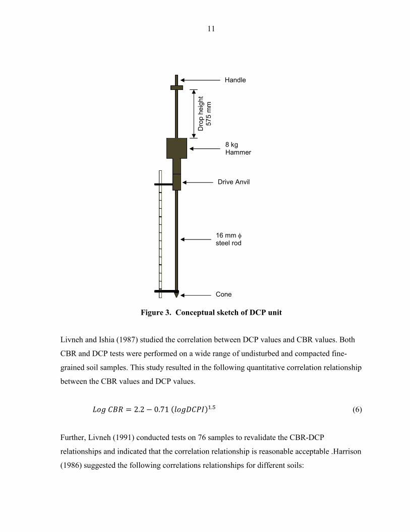
control and quality assurance testing. The DCP unit consists of a fixed 575 mm travel rod

with 8 kg dropping hammer, a lower rod containing a drive anvil; and a replaceable cone at

the end of the rod. A schematic of the DCP is shown in Figure 3. DCP tests are conducted by

dropping the hammer at the fixed drop height (575 mm) and recording the number of blows

versus depth. The test result is interpreted in terms of DCP index (DCPI) or penetration rate

(PR) with the unit of mm per blow.

The DCP is a simple test that characterizes the properties of pavement layers without digging

test pits or collecting soil samples. DCP tests can verify both the level and uniformity of

compaction (Burnham 1996; Siekmeier et al. 2000). Further, DCP tests results show the

thickness of the layer of soil of various profiles.

Several studies have been conducted to correlate DCPI with California Bearing Ratio (CBR)

based on empirical relationships. Kelyn (1975) developed Equation 4 based on 2,000

measurements.

������ � !"#! $ %"!&�'��(�)* (4)

Smith and Pratt (1983) and Riley et al. (1984) recommended Equation 5 based on field study.

������ � !"+# $ %"%+�'��(�)* (5)

11

Figure 3. Conceptual sketch of DCP unit

Livneh and Ishia (1987) studied the correlation between DCP values and CBR values. Both

CBR and DCP tests were performed on a wide range of undisturbed and compacted fine-

grained soil samples. This study resulted in the following quantitative correlation relationship

between the CBR values and DCP values.

������ � !"! $ ,"&%��'��(�)*��"- (6)

Further, Livneh (1991) conducted tests on 76 samples to revalidate the CBR-DCP

relationships and indicated that the correlation relationship is reasonable acceptable .Harrison

(1986) suggested the following correlations relationships for different soils:

Handle

8 kg Hammer

Drive Anvil

16 mm φ steel rod

Cone

Drop he

ight

575 mm

12

������ � !"+# $ %"%# ./0(�)* for clayey soil of DCPI > 10 mm/blow (7)

������ � !"&, $ %"%! ./0(�)* for granular soil of DCPI < 10 mm/blow (8)

The empirical relationship that was developed by the U.S. Army Corps of Engineers is

accepted by most researchers (Livneh 1995; Webster et al. 1992; Siekmeier et al. 2000; Chen

et al., 2001), and the equation for that relationship is shown as Equation 9:

������ � !"1& $ %"%! ./0(�)* or �� � !2! (�)*�"�3 (9)

Current study of correlating the DCPI and CBR are based on empirical relationship and the

correlation relationships are different for different field cases.

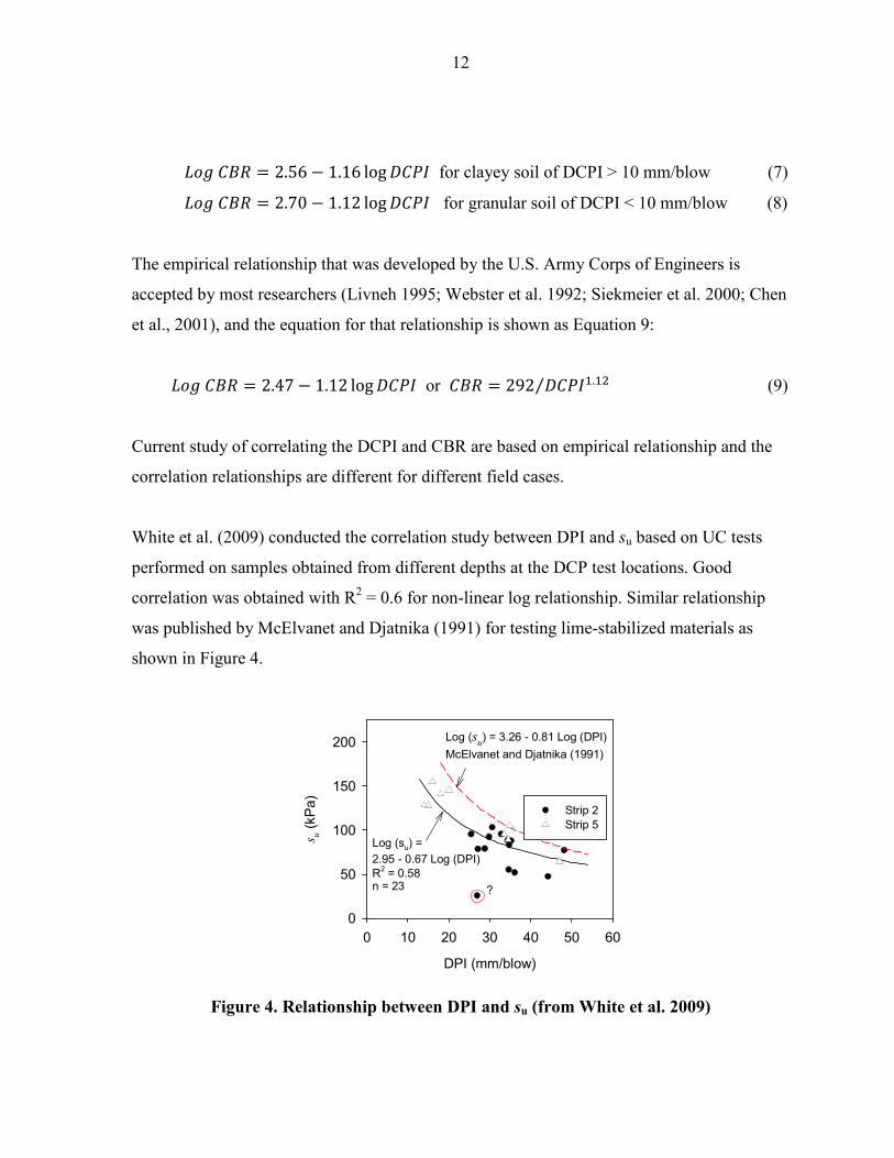
White et al. (2009) conducted the correlation study between DPI and su based on UC tests

performed on samples obtained from different depths at the DCP test locations. Good

correlation was obtained with R2 = 0.6 for non-linear log relationship. Similar relationship

was published by McElvanet and Djatnika (1991) for testing lime-stabilized materials as

shown in Figure 4.

Figure 4. Relationship between DPI and su (from White et al. 2009)

DPI (mm/blow)

0 10 20 30 40 50 60

s u (kP

a)

0

50

100

150

200

Strip 2Strip 5

Log (su) = 2.95 - 0.67 Log (DPI)R2 = 0.58n = 23 ?

Log (su) = 3.26 - 0.81 Log (DPI)

McElvanet and Djatnika (1991)

13

Influence of Soil Layering

Sridharan (1990) compared two methods for estimating the equivalent spring constant of a

layered system, which are the weighted average method and Odemark’s method. Tests were

conducted in two series: two-layer and three-layer systems using different materials. These

tests showed that the weighted average method more accurately predicts the equivalent

spring constant than Odemark’s method.

Poulos and Davis (1974) developed an approach for estimating the stress distribution under a

circular area (Equation 10), which can be explained as the applied load at the surface

multiplied by the influence factor. In this study, influence factor was also used to correlate

the surface reaction with different layers underneath.

σ4 � ) 5% $ 6 ���78��9

:;< (10)

where:

P = applied load at the surface,

a = radius of loading plate, and

z = depth from the surface.

Correlations between LWD and Other In Situ Point Measurements

Nazzal et al. (2004) conducted a study that correlated the Prima 100 model – LFWD with

other standard tests including the falling weight deflectometer (FWD) and the plate load test

(PLT). Good correlation was observed between ELWD and EFWD with a correlation coefficient

of 0.97, and a similar relationship was also obtained by Fleming (2001).

Vennapusa and White (2009) compared the Zorn LWD and PLT, and concluded that ELWD

had better correlation between the initial modulus (EV1) than reload modulus (EV2). Good

14

correlation between Zorn LWD and PLT was also obtained from Nazzal et al (2004), with

the correlation coefficient (R2) equal to 0.92 and 0.94 for EV1 and EV2, respectively.

Fleming et al. (2002) found that Zorn LWD consistently gave lower modulus than the other

devices, such as FWD and Prima LWD and perhaps because the accelerometer is mounted

within the bearing plate for Zorn LWD.

Target Value Determination for Quality Assurance

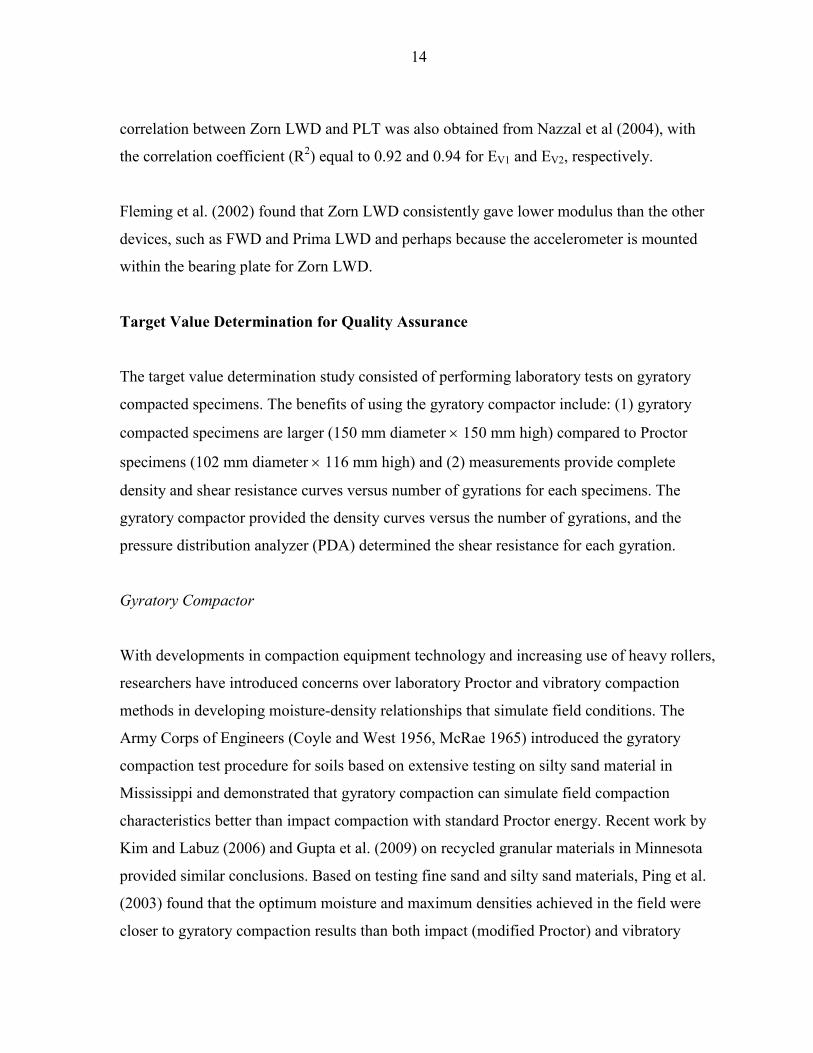
The target value determination study consisted of performing laboratory tests on gyratory

compacted specimens. The benefits of using the gyratory compactor include: (1) gyratory

compacted specimens are larger (150 mm diameter × 150 mm high) compared to Proctor

specimens (102 mm diameter × 116 mm high) and (2) measurements provide complete

density and shear resistance curves versus number of gyrations for each specimens. The

gyratory compactor provided the density curves versus the number of gyrations, and the

pressure distribution analyzer (PDA) determined the shear resistance for each gyration.

Gyratory Compactor

With developments in compaction equipment technology and increasing use of heavy rollers,

researchers have introduced concerns over laboratory Proctor and vibratory compaction

methods in developing moisture-density relationships that simulate field conditions. The

Army Corps of Engineers (Coyle and West 1956, McRae 1965) introduced the gyratory

compaction test procedure for soils based on extensive testing on silty sand material in

Mississippi and demonstrated that gyratory compaction can simulate field compaction

characteristics better than impact compaction with standard Proctor energy. Recent work by

Kim and Labuz (2006) and Gupta et al. (2009) on recycled granular materials in Minnesota

provided similar conclusions. Based on testing fine sand and silty sand materials, Ping et al.

(2003) found that the optimum moisture and maximum densities achieved in the field were

closer to gyratory compaction results than both impact (modified Proctor) and vibratory

15

compaction. According to Browne (2006), the gyratory compaction method produced

maximum dry unit weights greater than the modified Proctor method for three different types

of soils (A-1-a, A-3, and A-7-6), but the results depended on the number of gyrations and

compaction pressure.

The gyratory compaction method was standardized by ASTM (ASTM D-3387 Standard Test

Method for Compaction and Shear Properties of Bituminous Mixtures by Means of the U.S.

Corps of Engineers Gyratory Testing Machine (GTM)) based on the work by McRae (1965)

for its use for subgrade, base and asphalt mixtures. This method, however, has not been

widely implemented for compaction of subgrade and base materials. One reason for slow

implementation may be that no standard gyratory variables (e.g. gyration angle, number of

gyrations, normal stress, or rate of gyrations) have been developed for subgrade and subbase

materials.

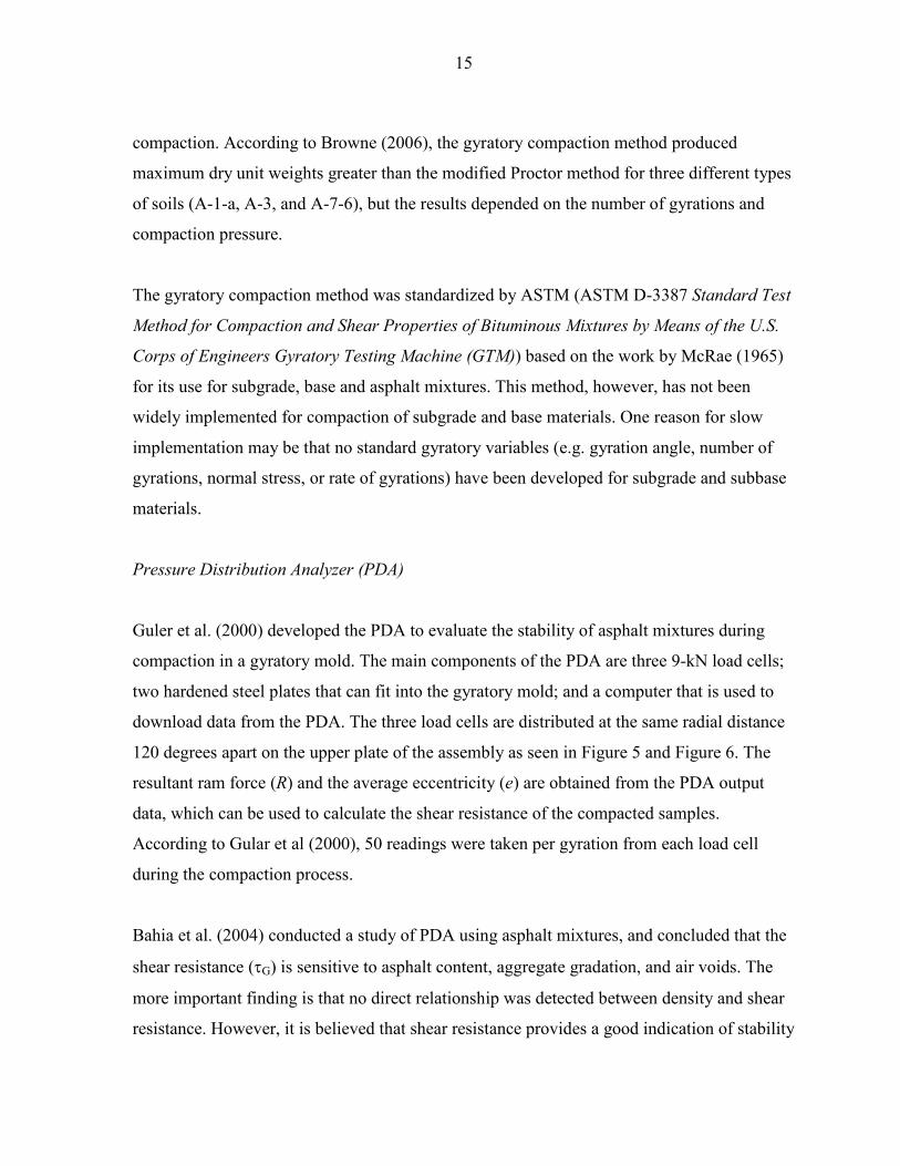
Pressure Distribution Analyzer (PDA)

Guler et al. (2000) developed the PDA to evaluate the stability of asphalt mixtures during

compaction in a gyratory mold. The main components of the PDA are three 9-kN load cells;

two hardened steel plates that can fit into the gyratory mold; and a computer that is used to

download data from the PDA. The three load cells are distributed at the same radial distance

120 degrees apart on the upper plate of the assembly as seen in Figure 5 and Figure 6. The

resultant ram force (R) and the average eccentricity (e) are obtained from the PDA output

data, which can be used to calculate the shear resistance of the compacted samples.

According to Gular et al (2000), 50 readings were taken per gyration from each load cell

during the compaction process.

Bahia et al. (2004) conducted a study of PDA using asphalt mixtures, and concluded that the

shear resistance (τG) is sensitive to asphalt content, aggregate gradation, and air voids. The

more important finding is that no direct relationship was detected between density and shear

resistance. However, it is believed that shear resistance provides a good indication of stability

16

of the compacted materials.

Figure 5. Pressure distribution analyzer (PDA)

Figure 6. PDA in the gyratory mold during gyration

1.07 c

m1.14 cm

0.76

cm

5.63 cm

5.63 c

m 5.63 cm

14.96 cm (original size)

14.96 cm (original size)

0.19 cm

CONNECTIONPINLOAD

CELL

UPPER AND LOWERHARDENED PLATES

120°

Mold Ram

PDA

Sample

1.25o

e

R

17

CHAPTER 3. TEST METHODS

This section summarizes the field and laboratory tests methods employed in the research and

the test standards followed. The descriptions of the standards for field and laboratory tests

were adopted from White et al. (2009).

Field Test Methods

Six field measurements devices are used in this research and the standard followed to

perform the field tests are summarized in Table 1.

Table 1. Summary of devices utilized in this research

Devices Standard followed

Nuclear gauge (NG) ASTM D2922-05

Light weight deflectometer (LWD) LWD Operation Manual (2000)

Falling weight deflectometer (FWD) KUAB 2m-FWD 150 Operation and Technical Reference Manual (2009)

Plate load test (PLT) ASTM D1195-93

Briaud compaction device (BCD) BCD Instruction Manual (2009)

Dynamic cone penetrometer (DCP) ASTM D6951-03

A calibrated nuclear moisture-density gauge (NG) device (Figure 7) was used to provide

rapid measurements of soil dry unit weight and moisture content. Tests were performed

following ASTM D2922-05 Test Method for Density of Soil and Soil Aggregate Inplace by

Nuclear Methods (Shallow Depth). Generally, two measurements of moisture and dry unit

weight were obtained at a particular location with the average value being reported. Probe

penetration depths were selected base on the compaction layer thickness.

18

Figure 7. Nuclear moisture-density gauge

LWD tests (Figure 8) with different device configurations were used to determine the

dynamic modulus at the surface. LWD tests were conducted in accordance with the

manufacture recommendations (Zorn 2003) for this research. The LWD modulus can be

determined using equation (11):

�

ELWD = =����>?��

�� @ A (11)

where, ELWD = elastic modulus (MPa), do = measured settlement (mm), v = Poisson’s ratio

(assumed to be 0.4 for this research), σo = applied stress (MPa), r = radius of the plate (mm)

and f = shape factor that depends on the stress. Vennapusa and White (2009) provide a

detailed description of the test methods for the equipment used in this study.

During this study, LWD tests were performed in the laboratory on the gyratory compacted

specimens. The compacted specimens were extruded from the gyratory mold and tested with

four different boundary conditions as shown in Figure 9: (a) no confinement, (b) confinement

with a soft polyurethane (Durometer = 20 A) sleeve, (c) confinement with a stiff

polyurethane (durometer = 50 A) sleeve, and (d) rigid confinement in the gyratory mold to

19

investigate the influence of boundary conditions. According to Vennapusa and White (2009),

the measuring range of the deflection transducer for Zorn LWD is 0.2 mm to 30 mm. The

measured deflections during laboratory target value determination study were ranging from

0.47 mm to 10.47 mm, which within the Zorn LWD measurement range.

Figure 8. Light weight deflectometer test with 200-mm diameter plate

Figure 9. LWD testing with four different boundary conditions: (a) no boundary, (b) soft polyurethane (Durometer = 20 A), (c) stiff polyurethane (Durometer = 50 A), and

(d) rigid gyratory compaction mold

(a) (b)

(c) (d)

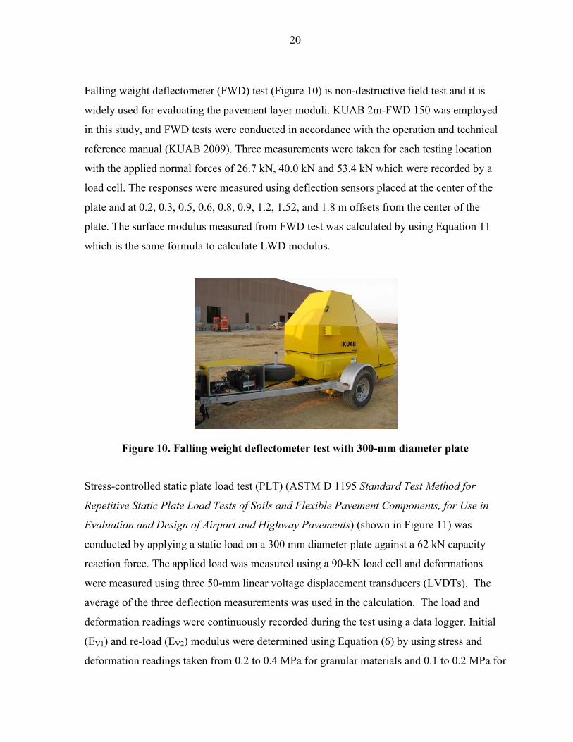
20

Falling weight deflectometer (FWD) test (Figure 10) is non-destructive field test and it is

widely used for evaluating the pavement layer moduli. KUAB 2m-FWD 150 was employed

in this study, and FWD tests were conducted in accordance with the operation and technical

reference manual (KUAB 2009). Three measurements were taken for each testing location

with the applied normal forces of 26.7 kN, 40.0 kN and 53.4 kN which were recorded by a

load cell. The responses were measured using deflection sensors placed at the center of the

plate and at 0.2, 0.3, 0.5, 0.6, 0.8, 0.9, 1.2, 1.52, and 1.8 m offsets from the center of the

plate. The surface modulus measured from FWD test was calculated by using Equation 11

which is the same formula to calculate LWD modulus.

Figure 10. Falling weight deflectometer test with 300-mm diameter plate

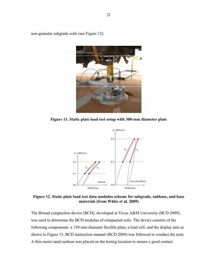
Stress-controlled static plate load test (PLT) (ASTM D 1195 Standard Test Method for

Repetitive Static Plate Load Tests of Soils and Flexible Pavement Components, for Use in

Evaluation and Design of Airport and Highway Pavements) (shown in Figure 11) was

conducted by applying a static load on a 300 mm diameter plate against a 62 kN capacity

reaction force. The applied load was measured using a 90-kN load cell and deformations

were measured using three 50-mm linear voltage displacement transducers (LVDTs). The

average of the three deflection measurements was used in the calculation. The load and

deformation readings were continuously recorded during the test using a data logger. Initial

(EV1) and re-load (EV2) modulus were determined using Equation (6) by using stress and

deformation readings taken from 0.2 to 0.4 MPa for granular materials and 0.1 to 0.2 MPa for

21

non-granular subgrade soils (see Figure 12).

Figure 11. Static plate load test setup with 300-mm diameter plate

Figure 12. Static plate load test data modulus scheme for subgrade, subbase, and base materials (from White et al. 2009)

The Briaud compaction device (BCD), developed at Texas A&M University (BCD 2009),

was used to determine the BCD modulus of compacted soils. The device consists of the

following components: a 150-mm diameter flexible plate, a load cell, and the display unit as

shown in Figure 13. BCD instruction manual (BCD 2009) was followed to conduct the tests.

A thin moist sand cushion was placed on the testing location to ensure a good contact

σ0 (MN/m2)

σ0 (MN/m2)

subgrade base and subbase

0.0

0.1

0.2

0.0

0.2

0.4

Deflection Deflection

EV1 EV2

EV1 EV2

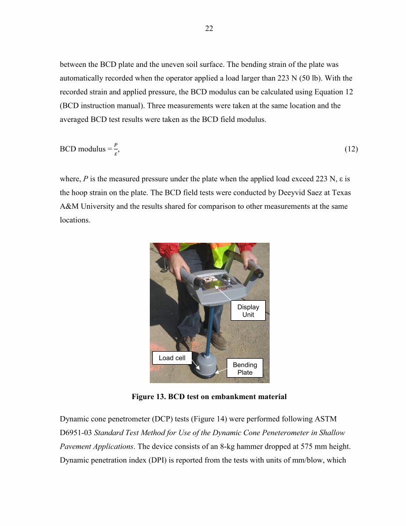
22

between the BCD plate and the uneven soil surface. The bending strain of the plate was

automatically recorded when the operator applied a load larger than 223 N (50 lb). With the

recorded strain and applied pressure, the BCD modulus can be calculated using Equation 12

(BCD instruction manual). Three measurements were taken at the same location and the

averaged BCD test results were taken as the BCD field modulus.

BCD modulus =�BC, (12)

where, P is the measured pressure under the plate when the applied load exceed 223 N, ε is

the hoop strain on the plate. The BCD field tests were conducted by Deeyvid Saez at Texas

A&M University and the results shared for comparison to other measurements at the same

locations.

Figure 13. BCD test on embankment material

Dynamic cone penetrometer (DCP) tests (Figure 14) were performed following ASTM

D6951-03 Standard Test Method for Use of the Dynamic Cone Peneterometer in Shallow

Pavement Applications. The device consists of an 8-kg hammer dropped at 575 mm height.

Dynamic penetration index (DPI) is reported from the tests with units of mm/blow, which

Bending Plate

Load cell

Display Unit

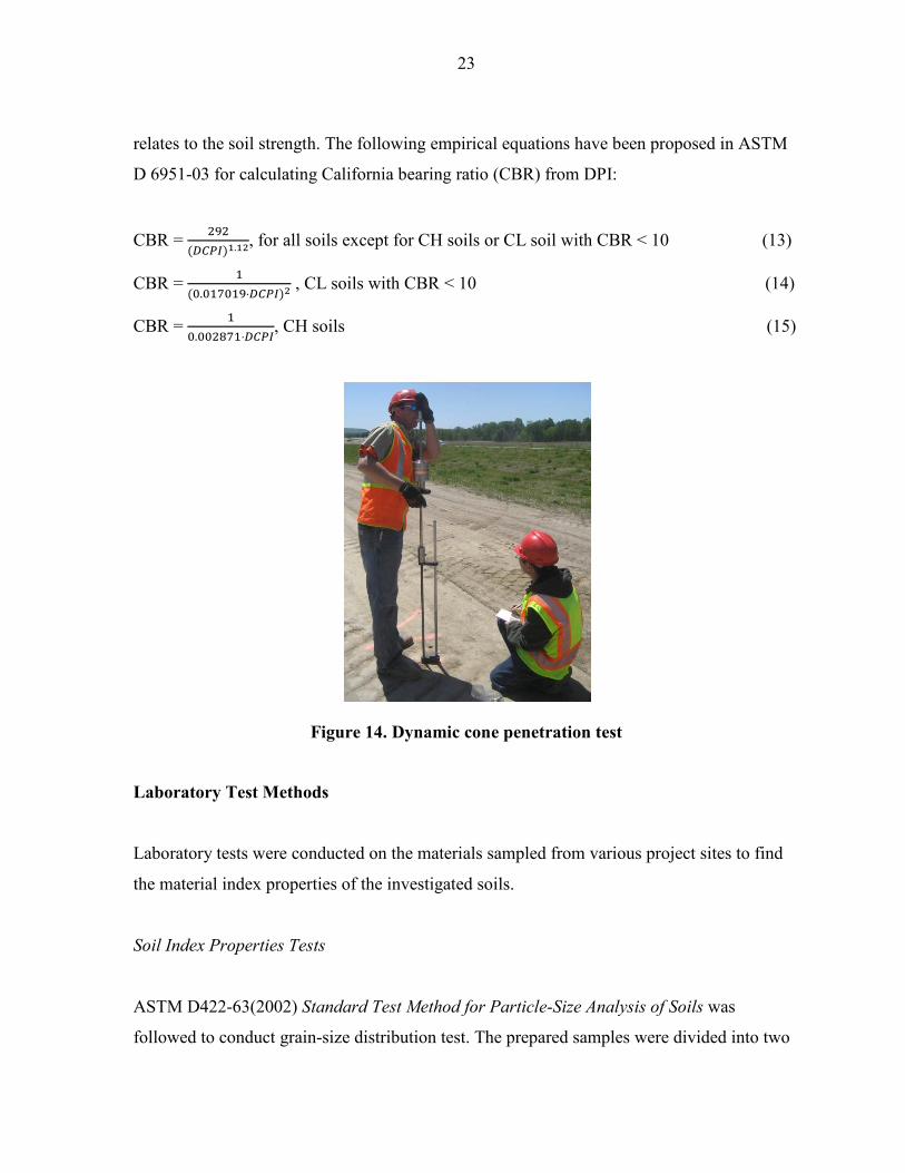
23

relates to the soil strength. The following empirical equations have been proposed in ASTM

D 6951-03 for calculating California bearing ratio (CBR) from DPI:

CBR =� D��EBF��"��, for all soils except for CH soils or CL soil with CBR < 10 (13)

CBR =� ��G"G�HG�D⋅�EBF�� , CL soils with CBR < 10 (14)

CBR =� �G"GGIH�⋅�EBF, CH soils (15)

Figure 14. Dynamic cone penetration test

Laboratory Test Methods

Laboratory tests were conducted on the materials sampled from various project sites to find

the material index properties of the investigated soils.

Soil Index Properties Tests

ASTM D422-63(2002) Standard Test Method for Particle-Size Analysis of Soils was

followed to conduct grain-size distribution test. The prepared samples were divided into two

24

portions by the No.10 sieve. Sieve analysis was performed on the portion washed and

retained on No. 10 sieve and hydrometer analysis was conducted on the portion passing the

No. 10 sieve using a 152 H hydrometer. After finishing the hydrometer test, the suspended

material was washed through the No. 200 sieve, oven dried, and then sieved through the No.

40 and No. 100 sieves.

Atterberg limits tests were performed in accordance with ASTM D4318-05 Standard Test

Methods for Liquid Limit, Plastic Limit, and Plasticity Index of Soils. The dry preparation

method was adopted and involved oven drying at a temperature below 60oC. Samples were

sieved through the No. 40 sieve before testing. Atterberg limits were used to classify the

material according to American Association of State Highway and Transportation Officials

(AASHTO) classification and Unified Soil Classification System (USCS).

ASTM D854-05 Standard Test Methods for Specific Gravity of Soil Solids by Water

Pycnometer was followed to conduct specific gravity tests. Method B – procedure for oven-

dried specimens was adopted for all the materials.

Laboratory Compaction Tests

The moisture content and dry density relationship for the investigated materials were

developed by performing standard and modified Proctor compaction tests. ASTM D698-00

and ASTM D1557-02 were followed for standard and modified Proctor tests, respectively.

Test method A was followed, and materials were air dried, sieved through the No.4 sieve,

and then moisture conditioned. The materials were stored in a moist condition for at least 16

hours prior to testing.

Relative density tests were performed on granular materials using a vibratory table. ASTM

D4253 Standard Test Methods for Maximum Index Density of Soils Using a Vibratory Table

and ASTM D 4254 Standard Test Methods for Minimum Index Density of Soils and

Calculation of Relative Density were followed to perform the compaction test to obtain the

25

maximum and minimum dry unit weights.

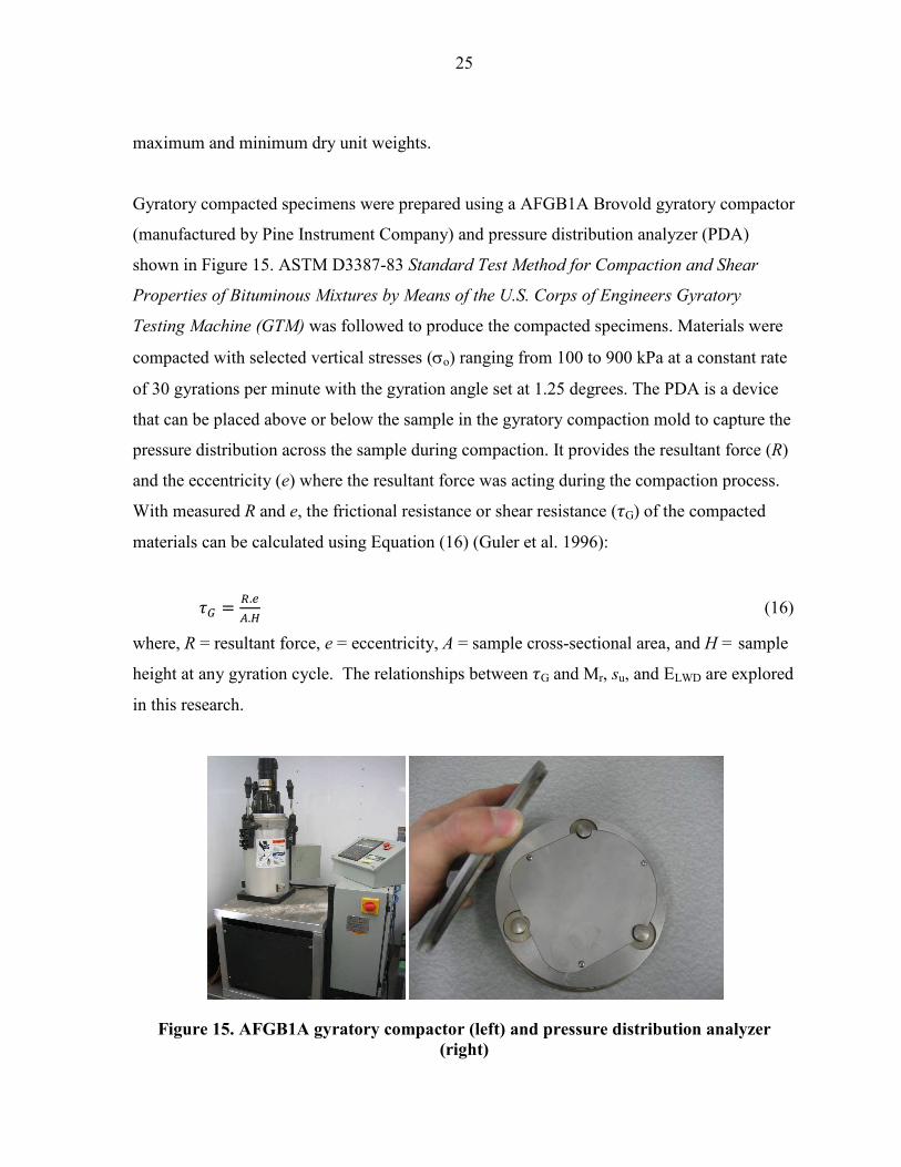
Gyratory compacted specimens were prepared using a AFGB1A Brovold gyratory compactor

(manufactured by Pine Instrument Company) and pressure distribution analyzer (PDA)

shown in Figure 15. ASTM D3387-83 Standard Test Method for Compaction and Shear

Properties of Bituminous Mixtures by Means of the U.S. Corps of Engineers Gyratory

Testing Machine (GTM) was followed to produce the compacted specimens. Materials were

compacted with selected vertical stresses (σo) ranging from 100 to 900 kPa at a constant rate

of 30 gyrations per minute with the gyration angle set at 1.25 degrees. The PDA is a device

that can be placed above or below the sample in the gyratory compaction mold to capture the

pressure distribution across the sample during compaction. It provides the resultant force (R)

and the eccentricity (e) where the resultant force was acting during the compaction process.

With measured R and e, the frictional resistance or shear resistance (JG) of the compacted

materials can be calculated using Equation (16) (Guler et al. 1996):

JK � L"MN"O (16)

where, R = resultant force, e = eccentricity, A = sample cross-sectional area, and H = sample

height at any gyration cycle. The relationships between JG and Mr, su, and ELWD are explored

in this research.

Figure 15. AFGB1A gyratory compactor (left) and pressure distribution analyzer (right)

26

Laboratory Strength Tests

Unconfined compressive (UC) tests (see Figure 16) were performed on the gyratory

compacted specimens in accordance with ASTM D2166 Standard Test Method for

Unconfined Compressive Strength of Cohesive Soil. In contrast with the ASTM standard, the

height-to-diameter ratio of the gyratory compacted specimens was approximately equal to

one instead of between 2 and 2.5. The strain rate for the UC tests was 1 %/min and loading

continued until 15 % strain was reached. Western Iowa loess (USCS: SL) was used in the

research to investigate the correlation between undrained shear strength (su) and shear

resistance (τG) from the gyratory compacted specimens.

Figure 16. Unconfined compressive test on gyratory compacted specimen

Resilient modulus (Mr) tests and unconsolidated-undrained triaxial compression (UU) tests

were performed on the gyratory compacted specimens in accordance with AASHTO T 307-

99 Standard Method of Test for Determining the Resilient Modulus of Soils and Aggregate

Materials and ASTM D 2850 Standard Test Method for Unconsolidated-Undrained Triaxial

Compression Test on Cohesive Soils. Specimens were prepared with the height to diameter

ratio H/D = 1:1 and H/D =2:1 to investigate the influence of the sample size on the resilient

modulus. The H/D=1:1 specimens (see Figure 17) were made using the gyratory compactor,

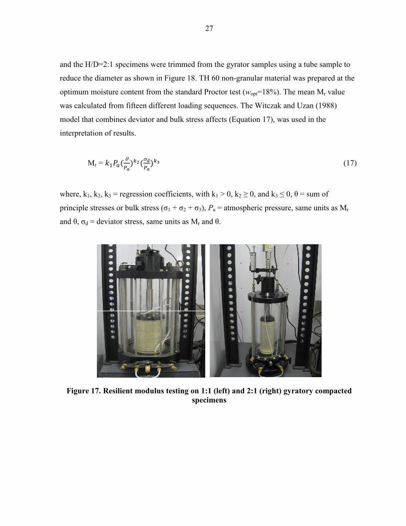
27

and the H/D=2:1 specimens were trimmed from the gyrator samples using a tube sample to

reduce the diameter as shown in Figure 18. TH 60 non-granular material was prepared at the

optimum moisture content from the standard Proctor test (wopt=18%). The mean Mr value

was calculated from fifteen different loading sequences. The Witczak and Uzan (1988)

model that combines deviator and bulk stress affects (Equation 17), was used in the

interpretation of results.

Mr = ��)P� θB7�Q��σRB7�QS (17)

where, k1, k2, k3 = regression coefficients, with k1 > 0, k2 ≥ 0, and k3 ≤ 0, θ = sum of

principle stresses or bulk stress (σ1 + σ2 + σ3), Pa = atmospheric pressure, same units as Mr

and θ, σd = deviator stress, same units as Mr and θ.

Figure 17. Resilient modulus testing on 1:1 (left) and 2:1 (right) gyratory compacted specimens

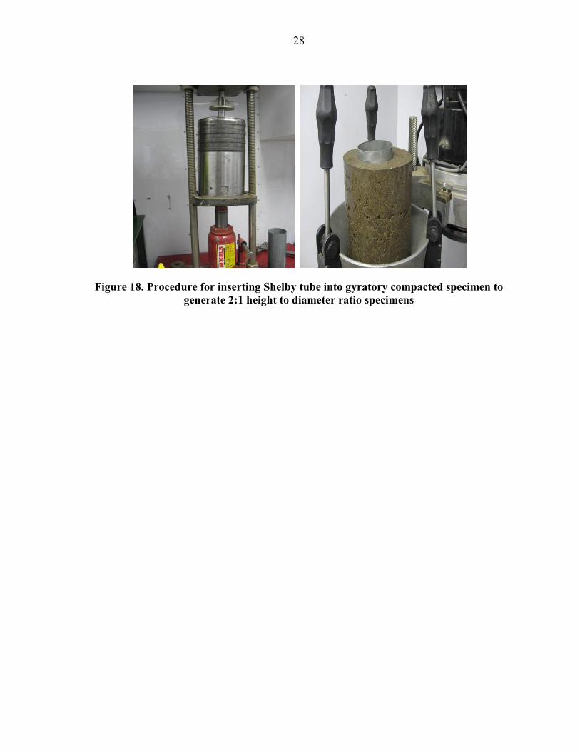
28

Figure 18. Procedure for inserting Shelby tube into gyratory compacted specimen to generate 2:1 height to diameter ratio specimens

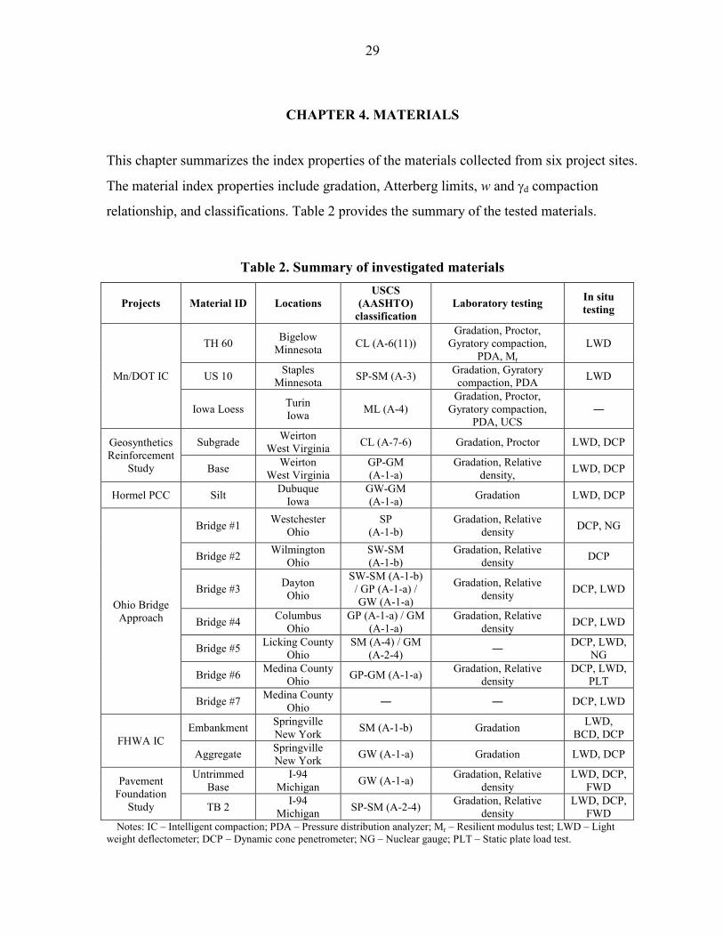
29

CHAPTER 4. MATERIALS

This chapter summarizes the index properties of the materials collected from six project sites.

The material index properties include gradation, Atterberg limits, w and γd compaction

relationship, and classifications. Table 2 provides the summary of the tested materials.

Table 2. Summary of investigated materials

Projects Material ID Locations USCS

(AASHTO) classification

Laboratory testing In situ testing

Mn/DOT IC

TH 60 Bigelow Minnesota CL (A-6(11))

Gradation, Proctor, Gyratory compaction,

PDA, Mr LWD

US 10 Staples Minnesota SP-SM (A-3) Gradation, Gyratory

compaction, PDA LWD

Iowa Loess Turin Iowa ML (A-4)

Gradation, Proctor, Gyratory compaction,

PDA, UCS ―

Geosynthetics Reinforcement

Study

Subgrade Weirton West Virginia CL (A-7-6) Gradation, Proctor LWD, DCP

Base Weirton West Virginia

GP-GM (A-1-a)

Gradation, Relative density, LWD, DCP

Hormel PCC Silt Dubuque Iowa

GW-GM (A-1-a) Gradation LWD, DCP

Ohio Bridge Approach

Bridge #1 Westchester Ohio

SP (A-1-b)

Gradation, Relative density DCP, NG

Bridge #2 Wilmington Ohio

SW-SM (A-1-b)

Gradation, Relative density DCP

Bridge #3 Dayton Ohio

SW-SM (A-1-b) / GP (A-1-a) / GW (A-1-a)

Gradation, Relative density DCP, LWD

Bridge #4 Columbus Ohio

GP (A-1-a) / GM (A-1-a)

Gradation, Relative density DCP, LWD

Bridge #5 Licking County Ohio

SM (A-4) / GM (A-2-4) ― DCP, LWD,

NG

Bridge #6 Medina County Ohio GP-GM (A-1-a) Gradation, Relative

density DCP, LWD,

PLT

Bridge #7 Medina County Ohio ― ― DCP, LWD

FHWA IC Embankment Springville

New York SM (A-1-b) Gradation LWD, BCD, DCP

Aggregate Springville New York GW (A-1-a) Gradation LWD, DCP

Pavement Foundation

Study

Untrimmed Base

I-94 Michigan GW (A-1-a) Gradation, Relative

density LWD, DCP,

FWD

TB 2 I-94 Michigan SP-SM (A-2-4) Gradation, Relative

density LWD, DCP,

FWD Notes: IC – Intelligent compaction; PDA – Pressure distribution analyzer; Mr – Resilient modulus test; LWD – Light weight deflectometer; DCP – Dynamic cone penetrometer; NG – Nuclear gauge; PLT – Static plate load test.

30

TH 60 – Bigelow

TH 60 subgrade material was sampled from Bigelow, Minnesota. The performed laboratory

tests include: grain-size distribution analysis, Atterberg limits tests, standard and modified

Proctor tests and gyratory compaction tests with the pressure distribution analyzer (PDA).

The material was classified as CL (lean clay sand) based on USCS classification and A-6(11)

from AASHTO classification (Figure 19). The Atterberg limits test results shown that the

liquid limit of the material is 39, plastic limit is 20 and plasticity index is 19. The maximum

dry unit weight and optimum moisture content for the modified Proctor test is 19.3 kN/m3

and 12.8% respectively; the maximum dry unit weight and optimum moisture content for the

standard Proctor test is 17.2 kN/m3 and 17.7 % respectively as shown in Figure 20. Table 3

summarizes the material index properties for this soil.

Gyratory compaction tests produced specimens for laboratory LWD tests with different

boundary conditions and resilient modulus tests with different sample sizes. PDA was placed

on the top of the gyratory compaction mold to capture the pressure distribution of the sample

during compaction process. Gyratory compaction tests were performed with 300 kPa applied

vertical pressure and 100 gyrations when producing the resilient modulus test specimens and

applied vertical pressures from 100 kPa to 600 kPa with 100 gyrations when producing the

LWD tests specimens. Figure 21 and Figure 22 provide the dry unit weight and shear

resistance versus number of gyrations and also the shear resistance versus degree of

saturation for this material. Based on τG versus degree of saturation curves, over-compaction

starts around 90% saturation for the samples with moisture content more than 16%.

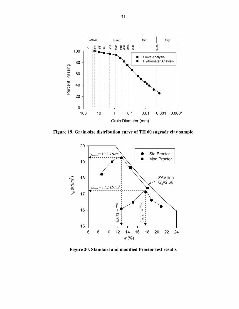
31

Figure 19. Grain-size distribution curve of TH 60 sugrade clay sample

Figure 20. Standard and modified Proctor test results

#10

#40

#100

#200

#43/8"

2" 0.00

2

SandGravel Silt Clay

Grain Diameter (mm)

0.00010.0010.010.1110100

Percent P

assing

0

20

40

60

80

100Sieve AnalysisHydrometer Analysis

1" 3/4"

#20

#60

w (%)6 8 10 12 14 16 18 20 22 24

γ d (kN

/m3 )

15

16

17

18

19

20

Std ProctorMod Proctor

ZAV lineGs=2.66

wopt = 17.7%

wopt = 12.8%

γdmax = 17.2 kN/m3

γdmax = 19.3 kN/m3

32

Table 3. Summary of the material properties for TH 60 non-granular soil

Parameter/Material TH 60 subgrade clay

Material Description Sandy lean clay

Maximum dry unit weight (kN/m3) and optimum moisture content (%) Standard Proctor 17.2 (17.7)

Modified Proctor 19.3 (12.8)

Gravel Content (%) (> 4.75mm) 3

Sand Content (%) (4.75mm – 75µm) 30

Silt Content (%) (75µm – 2µm) 38

Clay Content (%) (< 2µm) 29 Coefficient of Uniformity (cu) — Coefficient of Curvature (cc) — Liquid Limit, LL (%) 39

Plasticity Index, PI 19

AASHTO A-6(11) USCS CL Specific Gravity, Gs (Assumed) 2.66

33

Figure 21. Dry unit weight versus number of gyrations for TH 60 soil (USCS: CL)

Samples used for Mr testing

0 20 40 60 80 100

γ d (kN/m

3 )

13

14

15

16

17

18

19

σo = 600 kPa; H/D = 1:1 sample

σo = 600 kPa; H/D = 2:1 sample

σo = 300 kPa; H/D = 1:1 sample

σo= 300 kPa; H/D = 2:1 sample

σo = 100 kPa; H/D = 1:1 sample

σo = 100 kPa; H/D = 2:1 sample

Samples used for LWD No confinement testing

0 20 40 60 80 100

γ d (kN

/m3 )

13

14

15

16

17

18

19

Samples used for LWDSoft boundary testing

0 20 40 60 80 10013

14

15

16

17

18

19

Samples used for LWDStiff boundary testing

Number of Gyrations0 20 40 60 80 100

γ d (kN

/m3 )

13

14

15

16

17

18

19

Samples used for LWDRigid boundary testing

Number of Gyrations0 20 40 60 80 100

13

14

15

16

17

18

19

w = 17.5 %w = 17.2%

w = 18.0% w = 19.8%

w = 20.3% w = 21.8%

w = 15.4%

w = 16.0%w = 18.5%

w = 18.2%

w=12.4%

w=13.6%w = 12.4%

w = 15.3%

w = 18.5%

w = 18.4%

w = 15.9%

w = 15.4%

w = 12.5%w = 18.5%

w = 16.6%w = 18.0%

w = 15.5%

w = 15.5% w = 12.2%w = 14.3%

w = 15.4%

w = 17.6% w = 17.7%

w = 15.4%

Note: 1:1 and 2:1 H/D samples wereextracted for Mr and su testing

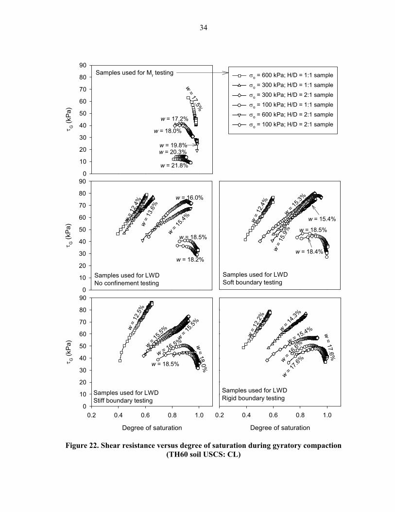
34

Figure 22. Shear resistance versus degree of saturation during gyratory compaction (TH60 soil USCS: CL)

Samples used for LWDNo confinement testing

τ G (kP

a)

0

10

20

30

40

50

60

70

80

90

Samples used for LWDSoft boundary testing

Samples used for LWDStiff boundary testing

Degree of saturation

0.2 0.4 0.6 0.8 1.0

τ G (kP

a)

0

10

20

30

40

50

60

70

80

90

Samples used for LWDRigid boundary testing

Degree of saturation

0.2 0.4 0.6 0.8 1.0

w = 12.4%

w = 13.6%

w = 16.0%

w = 15.4%

w = 18.5%

w = 18.2%w = 12.4%

w = 15.3%

w = 15.4%

w = 15.9% w = 18.5%

w = 18.4%

w = 12.5%

w = 15.5%

w = 15.5%

w = 1

6.5% w

= 18.0%w = 18.5%

w = 12.2%

w = 14.3%

w = 1

5.4%

w = 16.6%

w = 17.6%

w = 17.6%

Samples used for Mr testingτ G (kP

a)

0

10

20

30

40

50

60

70

80

90

σo = 600 kPa; H/D = 1:1 sample

σo = 300 kPa; H/D = 1:1 sample

σo = 300 kPa; H/D = 2:1 sample

σo = 100 kPa; H/D = 1:1 sample

σo = 600 kPa; H/D = 2:1 sample

σo = 100 kPa; H/D = 2:1 samplew = 17.2%

w = 19.8%

w = 18.0%

w = 17.5%

w = 20.3%

w = 21.8%

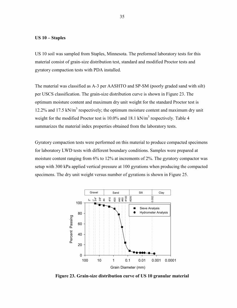
35

US 10 – Staples

US 10 soil was sampled from Staples, Minnesota. The preformed laboratory tests for this

material consist of grain-size distribution test, standard and modified Proctor tests and

gyratory compaction tests with PDA installed.

The material was classified as A-3 per AASHTO and SP-SM (poorly graded sand with silt)

per USCS classification. The grain-size distribution curve is shown in Figure 23. The

optimum moisture content and maximum dry unit weight for the standard Proctor test is

12.2% and 17.5 kN/m3 respectively; the optimum moisture content and maximum dry unit

weight for the modified Proctor test is 10.0% and 18.1 kN/m3 respectively. Table 4

summarizes the material index properties obtained from the laboratory tests.

Gyratory compaction tests were performed on this material to produce compacted specimens

for laboratory LWD tests with different boundary conditions. Samples were prepared at

moisture content ranging from 6% to 12% at increments of 2%. The gyratory compactor was

setup with 300 kPa applied vertical pressure at 100 gyrations when producing the compacted

specimens. The dry unit weight versus number of gyrations is shown in Figure 25.

Figure 23. Grain-size distribution curve of US 10 granular material

#10

#40

#100

#200

#43/8"

2" 0.00

2

SandGravel Silt Clay

Grain Diameter (mm)

0.00010.0010.010.1110100

Percent P

assing

0

20

40

60

80

100Sieve AnalysisHydrometer Analysis

1" 3/4"

#20

#60

36

Figure 24. Standard and modified Proctor test results for US 10 material

Table 4. Summary of the material properties for US 10 granular material

Parameter/Material US 10 granular material

Material Description Poorly graded sand with silt

Maximum dry unit weight (kN/m3) and optimum moisture content (%) Standard Proctor 17.5 (12.2)

Modified Proctor 18.1 (10.0)

Gravel Content (%) (> 4.75mm) 4

Sand Content (%) (4.75mm – 75µm) 87

Silt Content (%) (75µm – 2µm) 4

Clay Content (%) (< 2µm) 4 Coefficient of Uniformity (cu) 3.15 Coefficient of Curvature (cc) 1.15 Liquid Limit, LL (%) —

Plasticity Index, PI —

AASHTO A-3 USCS SP-SM Specific Gravity, Gs (Assumed) 2.68

w (%)0 2 4 6 8 10 12 14 16 18

γ d (kN

/m3 )

16.0

16.5

17.0

17.5

18.0

18.5

19.0

Std ProctorMod Proctor

ZAV lineGs=2.68

wopt = 12.2%

wopt = 10.0%

γdmax = 17.5 kN/m3

γdmax = 18.1 kN/m3

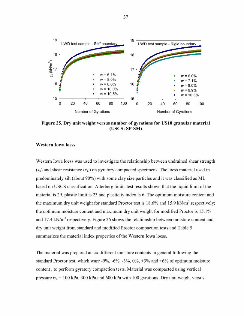
37

Figure 25. Dry unit weight versus number of gyrations for US10 granular material (USCS: SP-SM)

Western Iowa loess

Western Iowa loess was used to investigate the relationship between undrained shear strength

(su) and shear resistance (τG) on gyratory compacted specimens. The loess material used in

predominately silt (about 90%) with some clay size particles and it was classified as ML

based on USCS classification. Atterberg limits test results shown that the liquid limit of the

material is 29, plastic limit is 23 and plasticity index is 6. The optimum moisture content and

the maximum dry unit weight for standard Proctor test is 18.6% and 15.9 kN/m3 respectively;

the optimum moisture content and maximum dry unit weight for modified Proctor is 15.1%

and 17.4 kN/m3 respectively. Figure 26 shows the relationship between moisture content and

dry unit weight from standard and modified Proctor compaction tests and Table 5

summarizes the material index properties of the Western Iowa loess.

The material was prepared at six different moisture contents in general following the

standard Proctor test, which ware -9%, -6%, -3%, 0%, +3% and +6% of optimum moisture

content , to perform gyratory compaction tests. Material was compacted using vertical

pressure σo = 100 kPa, 300 kPa and 600 kPa with 100 gyrations. Dry unit weight versus

LWD test sample - Stiff boundary

Number of Gyrations

0 20 40 60 80 100

γ d (kN

/m3 )

15

16

17

18

19

w = 6.1%w = 8.0%w = 8.0%w = 10.0%w = 10.5%

LWD test sample - Rigid boundary

Number of Gyrations

0 20 40 60 80 10015

16

17

18

19

w = 6.0%w = 7.1%w = 8.0%w = 9.9%w = 10.3%

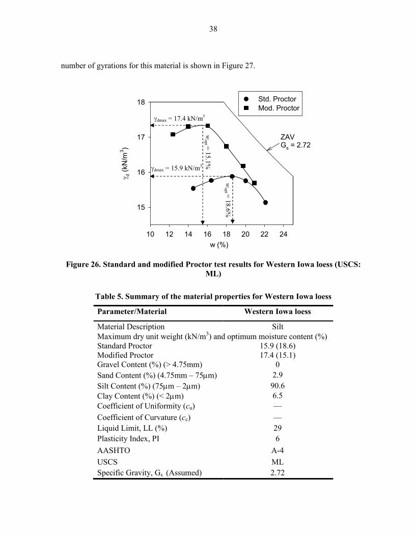
38

number of gyrations for this material is shown in Figure 27.

Figure 26. Standard and modified Proctor test results for Western Iowa loess (USCS: ML)

Table 5. Summary of the material properties for Western Iowa loess

Parameter/Material Western Iowa loess

Material Description Silt Maximum dry unit weight (kN/m3) and optimum moisture content (%) Standard Proctor 15.9 (18.6) Modified Proctor 17.4 (15.1) Gravel Content (%) (> 4.75mm) 0 Sand Content (%) (4.75mm – 75µm) 2.9 Silt Content (%) (75µm – 2µm) 90.6 Clay Content (%) (< 2µm) 6.5 Coefficient of Uniformity (cu) — Coefficient of Curvature (cc) — Liquid Limit, LL (%) 29 Plasticity Index, PI 6 AASHTO A-4 USCS ML Specific Gravity, Gs (Assumed) 2.72

w (%)10 12 14 16 18 20 22 24

γ d (kN

/m3 )

15

16

17

18 Std. ProctorMod. Proctor

ZAVGs = 2.72

γdmax = 17.4 kN/m3

γdmax = 15.9 kN/m3

wopt = 15.1%

wopt = 18.6%

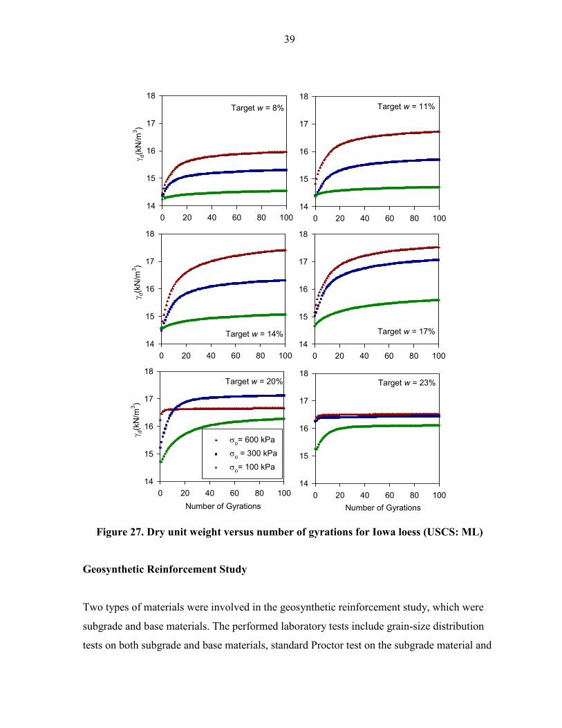
39

Figure 27. Dry unit weight versus number of gyrations for Iowa loess (USCS: ML)

Geosynthetic Reinforcement Study

Two types of materials were involved in the geosynthetic reinforcement study, which were

subgrade and base materials. The performed laboratory tests include grain-size distribution

tests on both subgrade and base materials, standard Proctor test on the subgrade material and

Target w = 8%

0 20 40 60 80 100

γ d(kN/m

3 )

14

15

16

17

18Target w = 11%

0 20 40 60 80 10014

15

16

17

18

Target w = 14%

0 20 40 60 80 100

γ d(kN/m

3 )

14

15

16

17

18

Target w = 17%

0 20 40 60 80 10014

15

16

17

18

Target w = 20%

Number of Gyrations

0 20 40 60 80 100

γ d(kN/m

3 )

14

15

16

17

18

σo= 600 kPa

σo = 300 kPa

σo= 100 kPa

Target w = 23%

Number of Gyrations

0 20 40 60 80 10014

15

16

17

18

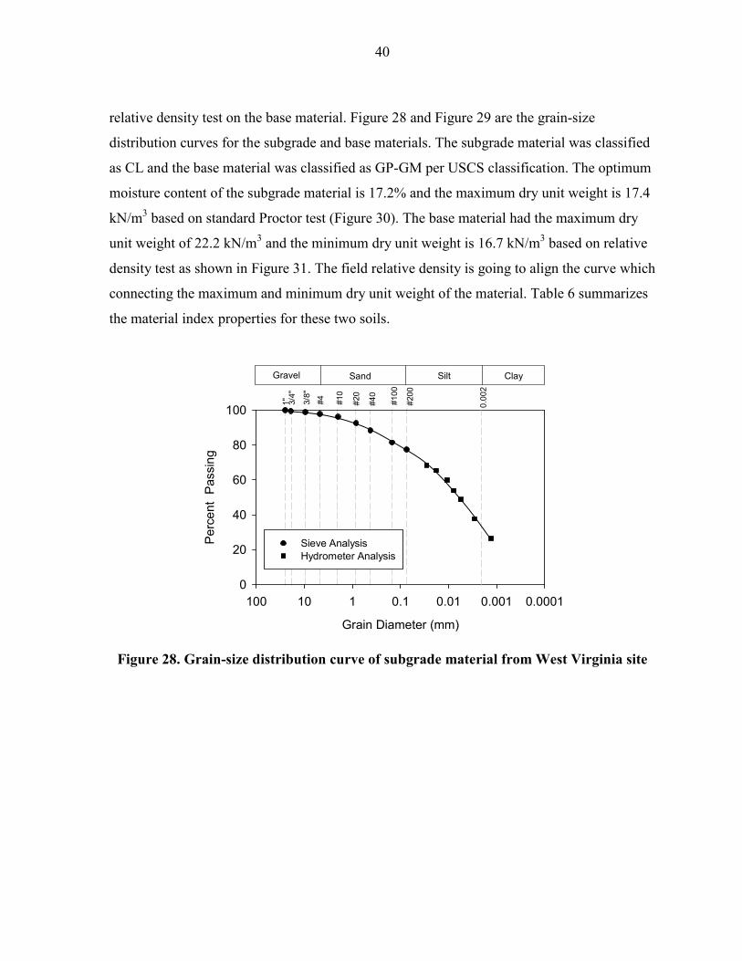
40

relative density test on the base material. Figure 28 and Figure 29 are the grain-size

distribution curves for the subgrade and base materials. The subgrade material was classified

as CL and the base material was classified as GP-GM per USCS classification. The optimum

moisture content of the subgrade material is 17.2% and the maximum dry unit weight is 17.4

kN/m3 based on standard Proctor test (Figure 30). The base material had the maximum dry

unit weight of 22.2 kN/m3 and the minimum dry unit weight is 16.7 kN/m3 based on relative

density test as shown in Figure 31. The field relative density is going to align the curve which

connecting the maximum and minimum dry unit weight of the material. Table 6 summarizes

the material index properties for these two soils.

Figure 28. Grain-size distribution curve of subgrade material from West Virginia site

#10

#40

#100

#200

#43/8"

0.00

2

SandGravel Silt Clay

Grain Diameter (mm)

0.00010.0010.010.1110100

Percent P

assing

0

20

40

60

80

100

Sieve AnalysisHydrometer Analysis

1" 3/4"

#20

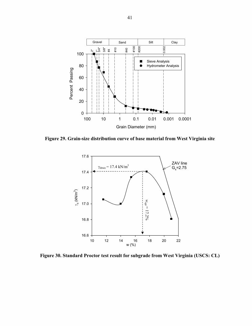
41

Figure 29. Grain-size distribution curve of base material from West Virginia site

Figure 30. Standard Proctor test result for subgrade from West Virginia (USCS: CL)

#10

#40

#100

#200

#43/8"

2" 0.002

SandGravel Silt Clay

Grain Diameter (mm)

0.00010.0010.010.1110100

Percent P

assing

0

20

40

60

80

100

Sieve AnalysisHydrometer Analysis

1" 3/4"

w (%)10 12 14 16 18 20 22

γ d (kN

/m3 )

16.6

16.8

17.0

17.2

17.4

17.6

ZAV lineGs=2.75

wopt = 17.2%

γdmax = 17.4 kN/m3

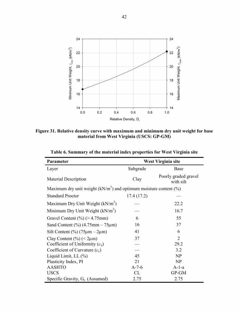
42

Figure 31. Relative density curve with maximum and minimum dry unit weight for base material from West Virginia (USCS: GP-GM)

Table 6. Summary of the material index properties for West Virginia site

Parameter West Virginia site

Layer Subgrade Base

Material Description Clay Poorly graded gravel with silt

Maximum dry unit weight (kN/m3) and optimum moisture content (%)

Standard Proctor 17.4 (17.2) —

Maximum Dry Unit Weight (kN/m3) — 22.2

Minimum Dry Unit Weight (kN/m3) — 16.7

Gravel Content (%) (> 4.75mm) 6 55 Sand Content (%) (4.75mm – 75µm) 16 37

Silt Content (%) (75µm – 2µm) 41 6

Clay Content (%) (< 2µm) 37 2 Coefficient of Uniformity (cu) — 29.2 Coefficient of Curvature (cc) — 3.2 Liquid Limit, LL (%) 45 NP Plasticity Index, PI 21 NP AASHTO A-7-6 A-1-a USCS CL GP-GM Specific Gravity, Gs (Assumed) 2.75 2.75

Relative Density, Dr

0.0 0.2 0.4 0.6 0.8 1.0

Minimum

Unit W

eigh

t, γ m

in (kN

/m3 )

14

16

18

20

22

24

Maximum

Unit W

eigh

t, γ m

ax (kN

/m3 )

14

16

18

20

22

24

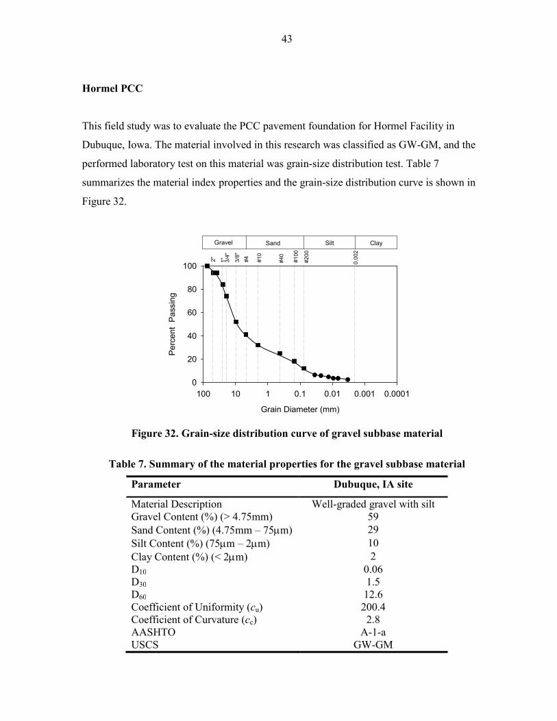
43

Hormel PCC

This field study was to evaluate the PCC pavement foundation for Hormel Facility in

Dubuque, Iowa. The material involved in this research was classified as GW-GM, and the

performed laboratory test on this material was grain-size distribution test. Table 7

summarizes the material index properties and the grain-size distribution curve is shown in

Figure 32.

Figure 32. Grain-size distribution curve of gravel subbase material

Table 7. Summary of the material properties for the gravel subbase material

Parameter Dubuque, IA site

Material Description Well-graded gravel with silt Gravel Content (%) (> 4.75mm) 59 Sand Content (%) (4.75mm – 75µm) 29 Silt Content (%) (75µm – 2µm) 10 Clay Content (%) (< 2µm) 2 D10 0.06 D30 1.5 D60 12.6 Coefficient of Uniformity (cu) 200.4 Coefficient of Curvature (cc) 2.8 AASHTO A-1-a USCS GW-GM

#10

#40

#100

#200

#43/8"

2" 0.002

SandGravel Silt Clay

Grain Diameter (mm)

0.00010.0010.010.1110100

Percent P

assing

0

20

40

60

80

100

1" 3/4"

44

Ohio Bridge Approach

The soil index properties of a total of 15 backfill material samples from bridge approaches at

seven project sites in Ohio were determined. Five of the samples were collected by the Ohio

Department of Transportation (ODOT), and 10 samples were collected by researchers from

Iowa State University (ISU). The ODOT samples were tested for grain-size distribution

(Table 8), and the ISU samples were tested for grain-size distribution, relative density, w and

γd, and laboratory collapse potential (Table 9).

Table 8. Summary of soil index properties for backfill materials (sampled by ODOT)

Description Location

Marzane at Perryville Shelly at Newark

West Mill Grove

Material ID Natural Sand type 1

Natural Sand type 2

Crushed Gravel

Natural Sand MF Sand

Gravel Content (%) (>4.75mm) 0.1 — 49.4 — 2.9

Sand Content (%) (4.75mm - 75 µm)

95.9 94.6 33.6 91.7 93.3

Fine Content (%) (< 75 µm)

4.0 5.4 17.0 8.3 3.8

Coefficient of Uniformity (Cu)

5.47 5.40 — 6.09 8.31

Coefficient of Curvature (Cc)

0.77 0.90 — 1.19 1.31

AASHTO A-1-b A-1-b A-1-b A-1-b A-1-b USCS SP SP-SM GM SW-SM SW

45

Table 9. Summary of soil index properties for backfill materials (sampled by ISU)

Description Bridge ID

BUT-75-0660 CL1-73-0985 MOT-75-1393

Material ID BUT Select Fill CL1 Sand MOT Sand MOT Pea

Gravel MOT Subbase

Gravel Content (%) (>4.75mm) — — 3 97 68

Sand Content (%) (4.75mm - 75 µm)

99 95 88 — 32

Fine Content (%) (< 75 µm)

1 5 9 3 —

Coefficient of Uniformity (cu)

3.15 7.09 6.83 1.76 23.06

Coefficient of Curvature (cc)

0.96 1.18 1.74 1.14 2.52

Maximum Dry Density (kg/m3) 1903.3 1914.8 1822.3 1652.3 2147.2

Minimum Dry Density (kg/m3) 1592.6 1475.5 1397.6 1499.6 1663.7

AASHTO A-1-b A-1-b A-1-b A-1-a A-1-a USCS SP SW-SM SW-SM GP GW

Description Bridge ID FRA-670-0904B LIC-37-1225L MED-71-0729

Material ID FRA Porous Backfill

FRA Subbase LIC EB- Till LIC WB-Till MED SB Gravel

Gravel Content (%) (>4.75mm) 95 43 24 39 49

Sand Content (%) (4.75mm - 75 µm)

1 33 35 34 44

Fine Content (%) (< 75 µm)

4 14 41 27 7

Coefficient of Uniformity (cu)

1.82 — — — 36.74

Coefficient of Curvature (cc)

1.16 — — — 0.84

Maximum Dry Density (kg/m3) 1609.8 1854.3 — — 2120.9

Minimum Dry Density (kg/m3) 1444.3 1535.3 — — 1670.4

Liquid Limit, LL (%) NP NP 23 24 NP Plasticity Index, PI NP NP 8 7 NP AASHTO A-1-a A-1-a A-4 A-2-4 A-1-a USCS GP GM SM GM GP-GM Note: No material collected from MED-71-075

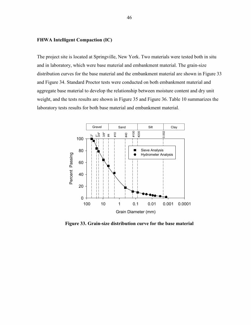
46

FHWA Intelligent Compaction (IC)

The project site is located at Springville, New York. Two materials were tested both in situ

and in laboratory, which were base material and embankment material. The grain-size

distribution curves for the base material and the embankment material are shown in Figure 33

and Figure 34. Standard Proctor tests were conducted on both embankment material and

aggregate base material to develop the relationship between moisture content and dry unit

weight, and the tests results are shown in Figure 35 and Figure 36. Table 10 summarizes the

laboratory tests results for both base material and embankment material.

Figure 33. Grain-size distribution curve for the base material

#10

#40

#100

#200

#43/8"

2" 0.002

SandGravel Silt Clay

Grain Diameter (mm)

0.00010.0010.010.1110100

Percent P

assing

0

20

40

60

80

100

Sieve AnalysisHydrometer Analysis

1" 3/4"

47

Figure 34. Grain-size distribution for the embankment material

Figure 35. Standard Proctor test result for embankment material

#10

#40

#100

#200

#43/8"

0.00

2

SandGravel Silt Clay

Grain Diameter (mm)

0.00010.0010.010.1110100

Percent P

assing

0

20

40

60

80

100

Sieve AnalysisHydrometer Analysis

1" 3/4"

w (%)0 2 4 6 8 10 12 14

γ d (kN

/m3 )

18

19

20

21

22

ZAVGs = 2.65

wopt = 8.6%

γd =20.5 kN/m3

48

Figure 36. Standard Proctor test result for aggregate base material

Table 10. Summary of material index properties from New York project site

Parameter Embankment Material

Aggregate Base

Maximum dry unit weight (kN/m3) and optimum moisture content (%)

Standard Proctor 20.5 (8.6) 21.2 (8.0)

Relative Density Test Results (oven-dry material)

γdmin (kN/m3) Not Performed

15.95

γdmax (kN/m3) 20.01

Gravel Content (%) (> 4.75mm) 24 46 Sand Content (%) (4.75mm – 75µm)

55 44

Silt Content (%) (75µm – 2µm) 15 7

Clay Content (%) (< 2µm) 6 3

Coefficient of Uniformity, cu 185.5 93.1

Coefficient of Curvature, cc 2.9 2.3

Liquid Limit, LL (%) 16 15

Plastic Limit, PL (%) Non-Plastic

AASHTO Classification A-1-b A-1-a

USCS Classification SM GW

Specific Gravity, Gs (Assumed) 2.65 2.75

w (%)0 2 4 6 8 10 12 14

γ d (kN

/m3 )

18

19

20

21

22

ZAVGs = 2.75

wopt = 8.0%

γd =21.2 kN/m3

49

Pavement Foundation Study

Three test beds were tested from the Michigan pavement foundation study. Test bed #1

consists of 40.6 cm of compacted and trimmed open-graded aggregate subbase over a

recompacted mixture of sand and silty clays. Test bed #2 was a section of 22.9 cm thick,

jointed concrete pavement constructed 40 years ago, and the material under the concrete

panel was sampled and transported to the laboratory to determine the grain-size distribution

and perform a standard Proctor test. Test bed #3 had the same material as test bed #1, which

is open-graded aggregate subbase material. The laboratory tests performed for the material

sampled from test bed #1 and #3 include grain-size distribution analysis and relative density

tests. The material sampled from test bed #1 was classified as GW and material sampled

from test bed #2 was classified as SP-SM per USCS classification. The grain-size distribution

curves for materials sampled from test bed #1 and #3 are shown in Figure 37 and Figure 38,

respectively. The standard Proctor test result for material sampled from test bed #2 is shown

in Figure 39 and the relative density test results for material from test bed #1 is shown in

Figure 40. Table 11 summarizes the laboratory tests results for both materials.

Figure 37. Grain-size distribution curve for the untrimmed base material (TB1&3)

#10

#40

#100

#200

#43/8"

11/2"

SandGravel

Grain Diameter (mm)

0.010.1110100

Percent P

assing

0

20

40

60

80

100

1" 3/4"

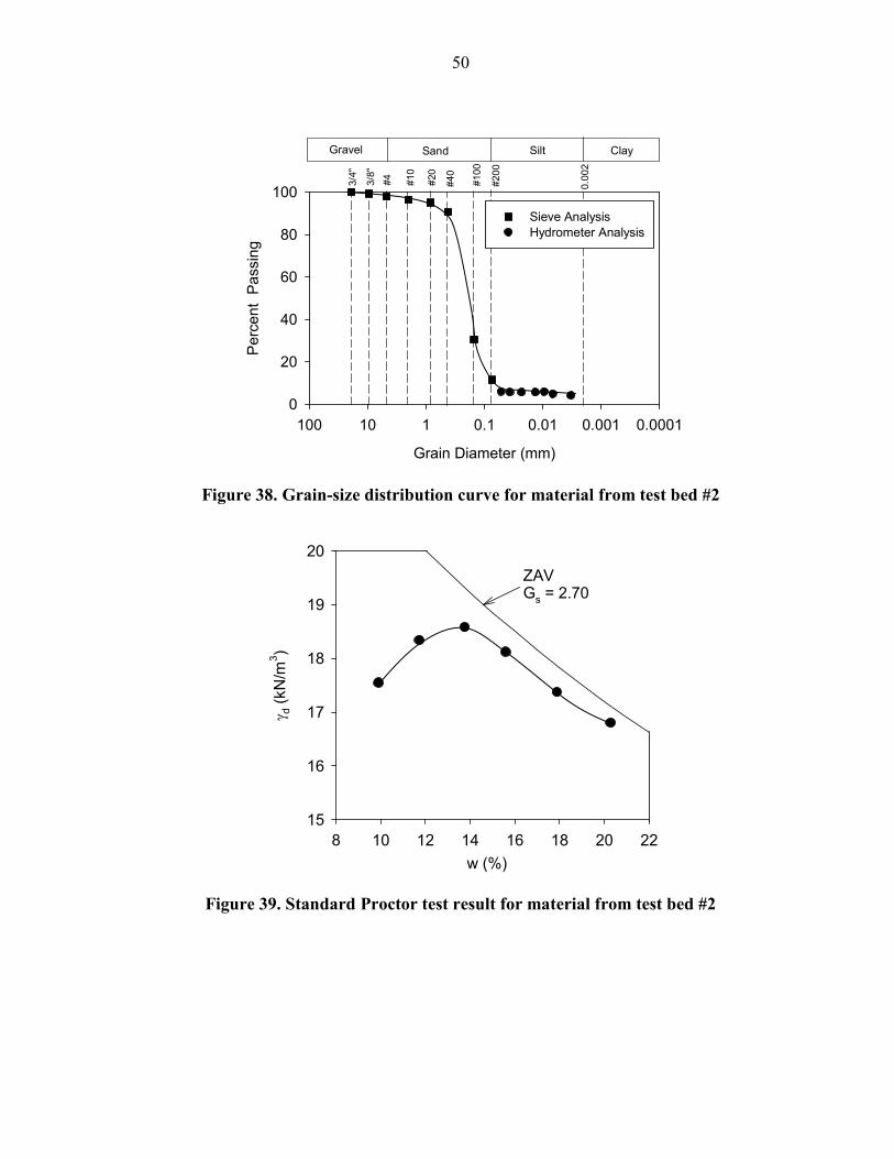
50

Figure 38. Grain-size distribution curve for material from test bed #2

Figure 39. Standard Proctor test result for material from test bed #2

#10

#40

#100

#200

#43/8"

0.00

2

SandGravel Silt Clay

Grain Diameter (mm)

0.00010.0010.010.1110100

Percent P

assing

0

20

40

60

80

100

Sieve AnalysisHydrometer Analysis

3/4"

#20

w (%)8 10 12 14 16 18 20 22

γ d (kN

/m3 )

15

16

17

18

19

20

ZAVGs = 2.70

51

Figure 40. Relative density curve with maximum and minimum dry unit weight for material from test bed #1

Table 11. Summary of soil index properties for the tested materials

Parameter Untrimmed Base TB2

Standard Proctor γdmax (kN/m3), wopt (%)

— 18.6 (13.8)

Maximum and minimum index density (kN/m3) 16.23 (14.04) —

Gravel Content (%) (> 4.75mm) 98 2.1 Sand Content (%) (4.75mm – 75µm)

— 86.5

Silt Content (%) (75µm – 2µm) 2 7.5

Clay Content (%) (< 2µm) — 3.9

D10 (mm) 13.44 0.069

D30 (mm) 19.57 0.149

D60 (mm) 26.18 0.243

Coefficient of Uniformity, cu 1.95 3.50

Coefficient of Curvature, cc 1.09 1.31

AASHTO Classification A-1-a A-2-4

USCS Classification GW SP-SM

Specific Gravity, Gs (Assumed) 2.75 2.65

Relative Density, Dr

0.0 0.2 0.4 0.6 0.8 1.0

Minimum

Unit W

eigh

t, γ m

in (kN

/m3 )

13

14

15

16

17

Maximum

Unit W

eigh

t, γ m

ax (kN

/m3 )

13

14

15

16

17

52

CHAPTER 5. TEST RESULTS AND DISCUSSION

This chapter presents and discusses the test results from both field and laboratory studies in

this order:

• case studies of field projects,

• the influence of LWD device configuration,

• correlations between LWD and other in situ point measurements,

• the influence of soil layering profiles on surface modulus,

• laboratory test results, and

• target value determination study for quality assurance.

Case Studies of Field Projects

Field studies were conducted at sites in West Virginia, Iowa, Ohio, New York, and

Michigan, to investigate the performance of five mechanistic-based compaction control

measurement devices and to use the devices to develop standard protocols for earthwork

QC/QA practices.

Geosynthetic Reinforcement Study

This field study was conducted at Weirton, West Virginia from March 17 to 20, 2009. The

goal for the field study was to evaluate the performance of three different geogrid

reinforcement materials. These materials were placed over relatively weak subgrade soils and

covered by aggregate base material. Four 18.3 m long sections each with 5 test points were

constructed, a control section and three sections labeled according to the geogrid material

used in each section (Figure 41 and Figure 42). Caterpillar and Case smooth drum rollers

(Figure 43) were used to compact the test beds. Nuclear gauge (NC), dynamic cone

penetrometer (DCP), light weight deflectometer (LWD) and plate load test (PLT) were

performed to determine the density, strength, and stiffness of the compacted materials. Two

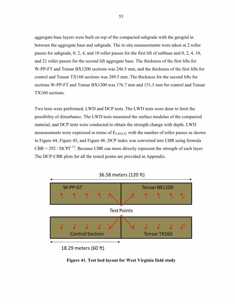
53

aggregate base layers were built on top of the compacted subgrade with the geogrid in

between the aggregate base and subgrade. The in situ measurements were taken at 2 roller

passes for subgrade, 0, 2, 4, and 10 roller passes for the first lift of subbase and 0, 2, 4, 10,

and 21 roller passes for the second lift aggregate base. The thickness of the first lifts for

W-PP-FT and Tensar BX1200 sections was 246.5 mm, and the thickness of the first lifts for

control and Tensar TX160 sections was 289.5 mm. The thickness for the second lifts for

sections W-PP-FT and Tensar BX1200 was 176.7 mm and 151.5 mm for control and Tensar

TX160 sections.

Two tests were performed, LWD and DCP tests. The LWD tests were done to limit the

possibility of disturbance. The LWD tests measured the surface modulus of the compacted

material, and DCP tests were conducted to obtain the strength change with depth. LWD

measurements were expressed in terms of ELWD-Z2 with the number of roller passes as shown

in Figure 44, Figure 45, and Figure 46. DCP index was converted into CBR using formula

CBR = 292 / DCPI1.12. Because CBR can more directly represent the strength of each layer.

The DCP-CBR plots for all the tested points are provided in Appendix.

Figure 41. Test bed layout for West Virginia field study

36.58 meters (120 ft)

18.29 meters (60 ft)

Tensar BX1200

Tensar TX160Control Section

W-PP-GT

Test Points

1 2 3 4 65 7 8 9 10

1 2 3 4 65 7 8 9 10

54

Figure 42. Overview of the site

Figure 43. Caterpillar (left) and Case (right) smooth drum rollers used in the West Virginia site

Control

W-PP-GT

TX160 BX1200

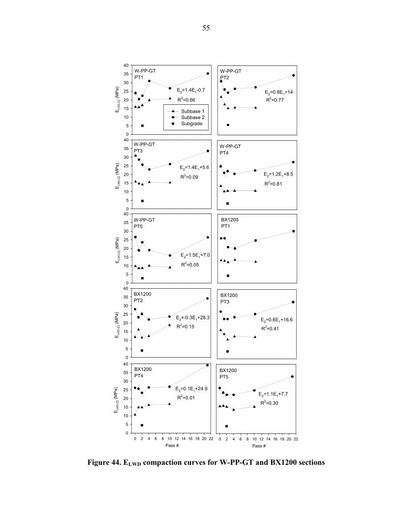
55

Figure 44. ELWD compaction curves for W-PP-GT and BX1200 sections

W-PP-GTPT1

ELW

D-Z2 (M

Pa)

0

5

10

15

20

25

30

35

40

Subbase 1Subbase 2Subgrade

ELW

D-Z2 (M

Pa)

0

5

10

15

20

25

30

35

40

ELW

D-Z2 (M

Pa)

0

5

10

15

20

25

30

35

40BX1200PT1

ELW

D-Z2 (M

Pa)

0

5

10

15

20

25

30

35

40

Pass #

0 2 4 6 8 10 12 14 16 18 20 22

ELW

D-Z2 (M

Pa)

0

5

10

15

20

25

30

35

40

Pass #

0 2 4 6 8 10 12 14 16 18 20 22

R2=0.66 R2=0.77

E2=1.4E1-0.7 E2=0.8E1+14

R2=0.09

E2=1.4E1+5.6

R2=0.81

E2=1.2E1+8.5

R2=0.05

E2=1.5E1+7.0

R2=0.15

E2=-0.3E1+28.3

R2=0.41

E2=0.6E1+16.6

R2=0.01

E2=0.1E1+24.9

R2=0.30

E2=1.1E1+7.7

W-PP-GTPT3

W-PP-GTPT4

W-PP-GTPT2

W-PP-GTPT5

BX1200PT2

BX1200PT3

BX1200PT4

BX1200PT5

56

Figure 45. ELWD compaction curves for control and TX160 section

ControlPT1

ELW

D-Z2 (M

Pa)

0

5

10

15

20

25

30

35

40

Subbase 1Subbase 2Subgrade

ELW

D-Z2 (M

Pa)

0

5

10

15

20

25

30

35

40

ELW

D-Z2 (M

Pa)

0

5

10

15

20

25

30

35

40

TX160PT1

ELW

D-Z2 (M

Pa)

0

5

10

15

20

25

30

35

40

Pass #0 2 4 6 8 10 12 14 16 18 20 22

ELW

D-Z2 (M

Pa)

0

5

10

15

20

25

30

35

40

Pass #

0 2 4 6 8 10 12 14 16 18 20 22

E2=0.1E1+28.3

R2=0.01

E2=-0.5E1+36.3

R2=0.07

E2=-0.1E1+33.5

R2=0.01E2=0.4E1+25.0

R2=0.01

E2=-3.3E1+74.7

R2=0.84E2=-0.9E1+38.1

R2=0.33

E2=0.9E1+14.0

R2=0.08

E2=-0.5E1+38.0

R2=0.36

E2=0.7E1+15.5

R2=0.72E2=0.3E1+20.2

R2=0.25

ControlPT2

ControlPT3

ControlPT4

ControlPT5

TX160PT2

TX160PT3

TX160PT4

TX160PT5

57

Figure 46. Averaged ELWD compaction curves for each section

The following key findings are withdrawn from this field case study:

• No significant improvement of LWD modulus for all sections when the roller passes

change from one to four, and the modulus of the base layer was clearly increased

after roller pass 21 times.

• The stiffness of the second base layer was significantly increased and no clear

evidence to prove the difference of using these geosynthetics.

Hormel PCC

A new Hormel facility with adjacent parking areas and driveways was under construction in

Dubuque, Iowa. Cracks had developed in sections of the recently completed pavement. Two

test sections were located, one in the paved driveway where the cracks had appeared and a

second in the unpaved loading dock area. The plan view in Figure 47 shows the in situ test

locations. FWD tests were performed on the paved driveway, and DCP and LWD tests were

Subbase 2

Pass #0 5 10 15 20

Subbase 1

Pass #

0 1 2 3 4 5 6 7 8 9 10 11

ELW

D-Z2 (M

Pa)

0

5

10

15

20

25

30

35

Averaged W-PP-GT sectionAveraged BX1200 sectionAveraged control sectionAveraged TX160 sectionAveraged W-PP-GT subgradeAveraged BX1200 subgradeAveraged control subgradeAveraged TX160 subgrade

58

conducted in the unpaved loading dock.

Figure 47. Plan view of in situ test locations, results of crack survey using GPS and cracks on the paved drive way (from White et al. 2009)

Before FWD data was collected from points on the paved driveway, three setting drops were

made to ensure that the loading plate was in good contact with the surface at each of the 45

points where the FWD tests were conducted to show the EFWD variance: these results are

shown in Figure 48.

Easting (ft)

15950 16000 16050 16100 16150 16200 16250 16300 16350 16400

Northing (ft)

16320

16340

16360

16380

16400

16420

Cracks2" Cores4" Cores/BoringsFWD Tests # 1-30FWD Tests # 31-45

Easting (ft)

15200 15400 15600 15800 16000 16200 16400

Northing (ft)

16300

16350

16400

16450

16500

16550

16600

16650CracksFWD Tests West-East Drive LaneFWD Tests East-West Drive LaneParking Lot Test Locations

Drive Way

Parking Lot

Test Lane (A) (B) (C) (D) Cha

venelle Court

Main Plant Building

# 1

# 28

# 21# 16 # 16 # 16

Average Gravel Subbase Thickness ~ 14 inches

Average Gravel subbase Thickness ~ 6 inches

# 1

# 20

# 1

# 17

# 1

# 19

Pavement Joints

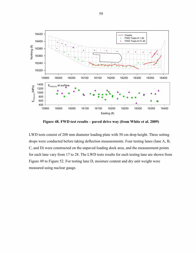
59

Figure 48. FWD test results – paved drive way (from White et al. 2009)

LWD tests consist of 200 mm diameter loading plate with 50 cm drop height. Three setting

drops were conducted before taking deflection measurements. Four testing lanes (lane A, B,

C, and D) were constructed on the unpaved loading dock area, and the measurement points

for each lane vary from 17 to 28. The LWD tests results for each testing lane are shown from

Figure 49 to Figure 52. For testing lane D, moisture content and dry unit weight were

measured using nuclear gauge.

Easting (ft)

15950 16000 16050 16100 16150 16200 16250 16300 16350 16400

EFWD-K3 (M

Pa)

400600800

100012001400

15950 16000 16050 16100 16150 16200 16250 16300 16350 16400

Northing (ft)

16320

16340

16360

16380

16400

16420 CracksFWD Tests # 1-30FWD Tests # 31-45

EFWD-K3 at surface

60

Figure 49. LWD, CBR, and subbase thickness (interpreted from DCP-CBR profiles)

measurements on testing lane A (tests on unpaved area granular subbase) (from White et al. 2009)

Distance (ft)

0 20 40 60 80 100 120 140

ELW

D-Z2 (M

Pa)

0

20

40

60

80

100

Testing Line (A)

(1)(2)

(3) (4)(5)

(6) (7) (8) (9)(10)

(11)

(12)(13)(14)

(15)(16)(17)(18)(19)

(20)

(21)

(22)(23)

(24)(25)

(26)(27)(28)

Distance (ft)

0 20 40 60 80 100 120 140

CBR (%)

0

20

40

60

80

100

Average CBR (Subbase)Average CBR (Subgrade)

Testing Line (A)

(1)(2) (3)

(4)(5)

(6)(7) (8) (9)

(10)

(11)

(12)(13) (14)(15)(16)(17)(18)(19)

(20)

(21)(22)

(23)(24)(25)(26) (27)

(28)

Distance (ft)

0 20 40 60 80 100 120 140

Subba

se Thickne

ss (in)

0

5

10

15

20

25

30

Testing Line (A)

(1) (2) (3) (4)(5) (6) (7) (8) (9)(10)

(11)(12)(13)(14)

(15)(16)(17)(18)(19)

(20)

(21)(22)

(23)(24) (25)

(26) (27) (28)

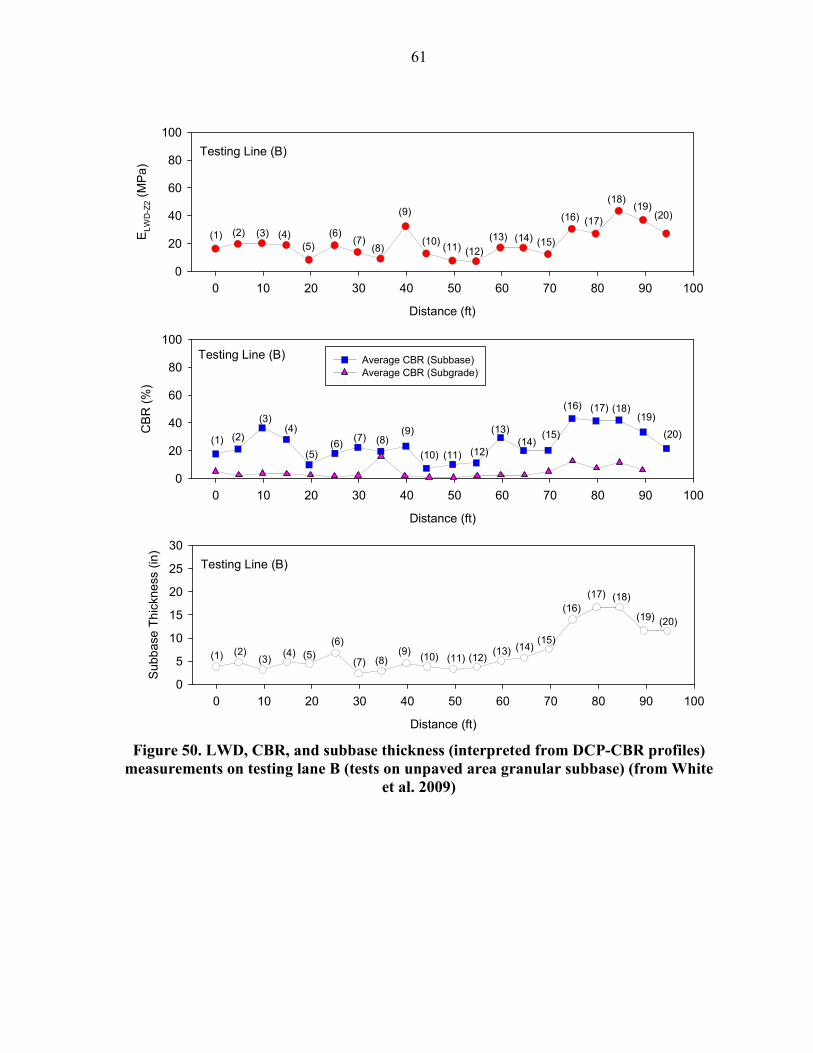
61

Figure 50. LWD, CBR, and subbase thickness (interpreted from DCP-CBR profiles)

measurements on testing lane B (tests on unpaved area granular subbase) (from White et al. 2009)

Distance (ft)

0 10 20 30 40 50 60 70 80 90 100

ELW

D-Z2 (M

Pa)

0

20

40

60

80

100

Testing Line (B)

(1) (2) (3) (4)(5)

(6)(7)

(8)

(9)

(10) (11) (12)(13) (14) (15)

(16) (17)

(18)(19)

(20)

Distance (ft)

0 10 20 30 40 50 60 70 80 90 100

CBR (%)

0

20

40

60

80

100

Average CBR (Subbase)Average CBR (Subgrade)

Testing Line (B)

(1) (2)

(3)(4)

(5)(6)

(7) (8)(9)

(10) (11) (12)

(13)(14)

(15)

(16) (17) (18)(19)

(20)

Distance (ft)

0 10 20 30 40 50 60 70 80 90 100

Sub

base Thickne

ss (in)

0

5

10

15

20

25

30

Testing Line (B)

(1) (2)(3)

(4) (5)(6)

(7) (8)(9) (10) (11) (12)

(13) (14)(15)

(16)(17) (18)

(19) (20)

62

Figure 51. LWD, CBR, and subbase thickness (interpreted from DCP-CBR profiles)

measurements on testing lane C (tests on unpaved area granular subbase) (from White et al. 2009)

Distance (ft)

0 10 20 30 40 50 60 70 80 90 100

ELW

D-Z2 (M

Pa)

0

20

40

60

80

100

Testing Line (C)

(1)(2)

(3) (4)(5)

(6) (7)

(8)

(9)

(10) (11)(12) (13) (14)

(15)

(16) (17)

Distance A vs ELWD-Z2 (MPa)

Distance (ft)

0 10 20 30 40 50 60 70 80 90 100

CBR (%)

0

20

40

60

80

100Average CBR (Subbase)Average CBR (Subgrade)

Testing Line (C)

(1)(2)

(3)

(4)(5)

(6)(7)

(8)

(9)

(10) (11) (12) (13)(14)

(15)

(16) (17)

Distance (ft)

0 10 20 30 40 50 60 70 80 90 100

Sub

base Thickness (in)

0

5

10

15

20

25

30

Testing Line (C)

(1) (2) (3)(4) (5) (6) (7) (8) (9)

(10)(11)

(12) (13)(14) (15)

(16)(17)

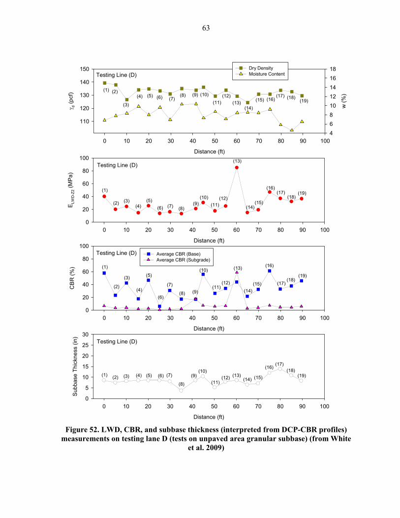
63

Figure 52. LWD, CBR, and subbase thickness (interpreted from DCP-CBR profiles)

measurements on testing lane D (tests on unpaved area granular subbase) (from White et al. 2009)

Distance (ft)

0 10 20 30 40 50 60 70 80 90 100

ELW

D-Z2 (M

Pa)

0

20

40

60

80

100Testing Line (D)

(1)

(2) (3)(4)

(5)

(6) (7) (8)(9)

(10)

(11)(12)

(13)

(14)(15)

(16)(17)

(18)(19)

Distance (ft)

0 10 20 30 40 50 60 70 80 90 100

γ d (pcf)

110

120

130

140

150

w (%)

4

6

8

10

12

14

16

18Dry DensityMoisture ContentTesting Line (D)

(1) (2)

(3)

(4) (5) (6) (7)(8) (9) (10)

(11)(12)

(13)(14)

(15) (16)(17) (18)

(19)

Distance A vs ELWD-Z2 (MPa)

Distance (ft)

0 10 20 30 40 50 60 70 80 90 100

CBR (%)

0

20

40

60

80

100Average CBR (Base)Average CBR (Subgrade)

Testing Line (D)

(1)

(2)

(3)

(4)

(5)

(6)

(7)

(8) (9)

(10)

(11)(12)

(13)

(14)(15)

(16)

(17)

Distance (ft)

0 10 20 30 40 50 60 70 80 90 100

Sub

base Thickne

ss (in)

0

5

10

15

20

25

30Testing Line (D)

(1) (2) (3) (4) (5) (6) (7)

(8)

(9)(10)

(11)(12) (13)

(14) (15)

(16)(17)

(18)(19)

(18)(19)

64

DCP tests were performed after LWD test to avoid the disturbance caused by previous tests

for the testing points. The DCP tests results were interpreted in terms of CBR which can

present the strength of the tested soil more directly. The DCP-CBR tests results are shown

from Figure 53 to Figure 56.

Figure 53. DCP-CBR profiles on testing lane A – unpaved area granular subbase (from

White et al. 2009)

CBR (%)

0 30 60 90 120

Dep

th (ft)

0.0

0.5

1.0

1.5

2.0

2.5

3.0

(1)(2)(3)(4)(5)

CBR (%)

0 30 60 90 1200.0

0.5

1.0

1.5

2.0

2.5

3.0

(6)(7)(8)(9)(10)

CBR (%)

0 30 60 90 1200.0

0.5

1.0

1.5

2.0

2.5

3.0

(11)(12)(13)(14)(15)

CBR (%)

0 30 60 90 120

Dep

th (ft)

0.0

0.5

1.0

1.5

2.0

2.5

3.0

(16)(17)(18)(19)(20)

CBR (%)

0 30 60 90 1200.0

0.5

1.0

1.5

2.0

2.5

3.0

(21)(22)(23)(24)(25)

CBR (%)

0 30 60 90 1200.0

0.5

1.0

1.5

2.0

2.5

3.0

(26)(27)(28)

Testing Lane A

# 1 # 28

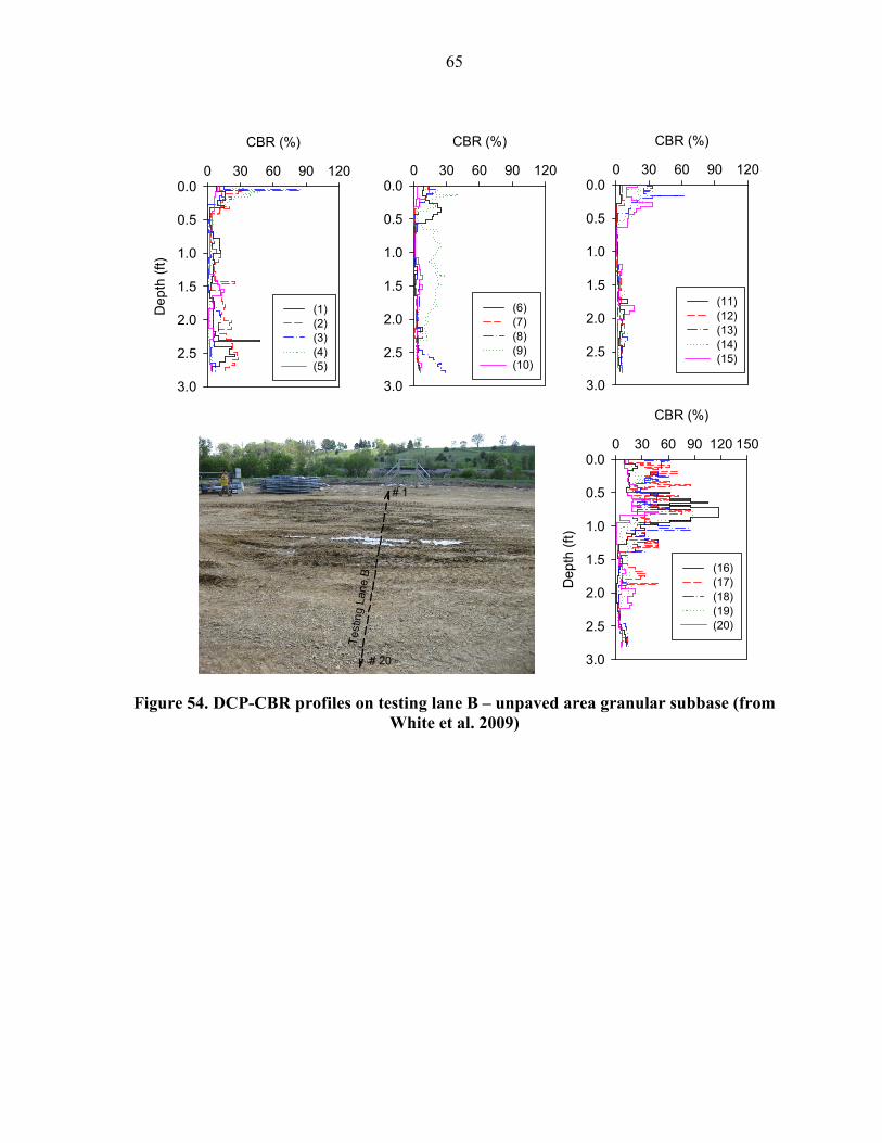
65

Figure 54. DCP-CBR profiles on testing lane B – unpaved area granular subbase (from

White et al. 2009)

CBR (%)

0 30 60 90 120Dep

th (ft)

0.0

0.5

1.0

1.5

2.0

2.5

3.0

(1)(2)(3)(4)(5)

CBR (%)

0 30 60 90 1200.0

0.5

1.0

1.5

2.0

2.5

3.0

(6)(7)(8)(9)(10)

CBR (%)

0 30 60 90 1200.0

0.5

1.0

1.5

2.0

2.5

3.0

(11)(12)(13)(14)(15)

CBR (%)

0 30 60 90 120 150

Dep

th (ft)

0.0

0.5

1.0

1.5

2.0

2.5

3.0

(16)(17)(18)(19)(20)

# 1

# 20

Testing Lane B

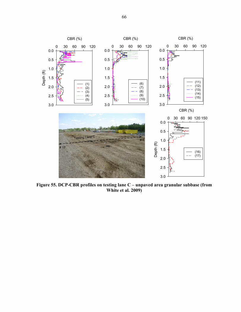
66

Figure 55. DCP-CBR profiles on testing lane C – unpaved area granular subbase (from

White et al. 2009)

CBR (%)

0 30 60 90 120Dep

th (ft)

0.0

0.5

1.0

1.5

2.0

2.5

3.0

(1)(2)(3)(4)(5)

CBR (%)

0 30 60 90 1200.0

0.5

1.0

1.5

2.0

2.5

3.0

(6)(7)(8)(9)(10)

CBR (%)

0 30 60 90 1200.0

0.5

1.0

1.5

2.0

2.5

3.0

(11)(12)(13)(14)(15)

CBR (%)

0 30 60 90 120 150

Dep

th (ft)

0.0

0.5

1.0

1.5

2.0

2.5

3.0

(16)(17)

# 1

# 17

Testing Lane C

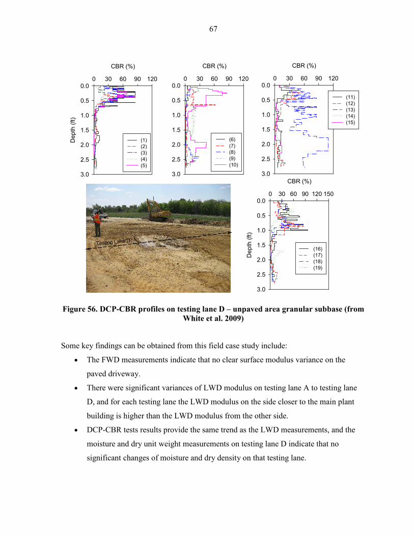
67

Figure 56. DCP-CBR profiles on testing lane D – unpaved area granular subbase (from

White et al. 2009)

Some key findings can be obtained from this field case study include:

• The FWD measurements indicate that no clear surface modulus variance on the

paved driveway.

• There were significant variances of LWD modulus on testing lane A to testing lane

D, and for each testing lane the LWD modulus on the side closer to the main plant

building is higher than the LWD modulus from the other side.

• DCP-CBR tests results provide the same trend as the LWD measurements, and the

moisture and dry unit weight measurements on testing lane D indicate that no

significant changes of moisture and dry density on that testing lane.

CBR (%)

0 30 60 90 120Dep

th (ft)

0.0

0.5

1.0

1.5

2.0

2.5

3.0

(1)(2)(3)(4)(5)

CBR (%)

0 30 60 90 1200.0

0.5

1.0

1.5

2.0

2.5

3.0

(6)(7)(8)(9)(10)

CBR (%)

0 30 60 90 1200.0

0.5

1.0

1.5

2.0

2.5

3.0

(11)(12)(13)(14)(15)

CBR (%)

0 30 60 90 120 150

Dep

th (ft)

0.0

0.5

1.0

1.5

2.0

2.5

3.0

(16)(17)(18)(19)

Testing Lane D

68

Ohio Bridge Approach

The purpose of this field study was to characterize the backfill materials of the new bridge

approach in Ohio area. Seven new bridges were investigated during this field study and the

summary of the project locations is provided in Table 12. The geotechnical investigations for

this project consist of field testing and laboratory testing. The field testing including:

density/moisture measurement using nuclear gauge, elastic modulus measurement by

performing LWD tests and PLTs, and strength measurement by conducting DCP tests.

Laboratory tests were performed on the representative samples which were transported to the

laboratory from the field, and the laboratory tests include grain-size distribution tests, relative

density tests, standard Proctor test, and collapse potential test.

Table 12. Summary of in situ testing at different bridge locations

Bridge number Date Bridge ID

(SFN) Location In situ testing

#1 5/14/2009 BUT-75-0660 (0901822) Westchester, Ohio DCP, NG

#2 5/14/2009 CL1-73-0985 (1402293) Wilmington, Ohio DCP

#3 5/14/2009 MOT-75-1393 (5708443) Dayton, Ohio DCP, LWD

#4 5/15/2009 FRA-670-0904B (2517949) Columbus, Ohio DCP, LWD

#5 5/15/2009 LIC-37-1225L (4501691L) Licking County, Ohio DCP, LWD,

NG

#6 5/16/2009 MED-71-0729 (5202809) Medina County, Ohio DCP, LWD,

PLT

#7 5/16/2009 MED-71-0750 (5204275) Medina County, Ohio DCP, LWD

Note: SFN – Structural file number; DCP – Dynamic cone penetrometer; NG – Nuclear moisture – density gauge; LWD –200-mm plate diameter zorn light weight deflectometer, PLT – 300-mm diameter static plate load test

Bridge # 1 is located at the I-75 & SR 129 interchange in West Chester, Ohio. Mechanically

Stabilized Earth (MSE) walls were built on spread footing foundations on the North-East

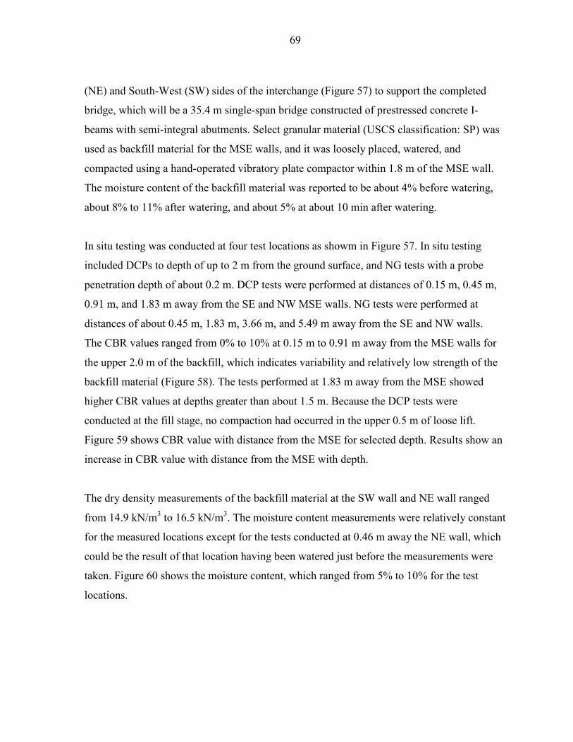
69

(NE) and South-West (SW) sides of the interchange (Figure 57) to support the completed

bridge, which will be a 35.4 m single-span bridge constructed of prestressed concrete I-

beams with semi-integral abutments. Select granular material (USCS classification: SP) was

used as backfill material for the MSE walls, and it was loosely placed, watered, and

compacted using a hand-operated vibratory plate compactor within 1.8 m of the MSE wall.

The moisture content of the backfill material was reported to be about 4% before watering,

about 8% to 11% after watering, and about 5% at about 10 min after watering.

In situ testing was conducted at four test locations as showm in Figure 57. In situ testing

included DCPs to depth of up to 2 m from the ground surface, and NG tests with a probe

penetration depth of about 0.2 m. DCP tests were performed at distances of 0.15 m, 0.45 m,

0.91 m, and 1.83 m away from the SE and NW MSE walls. NG tests were performed at

distances of about 0.45 m, 1.83 m, 3.66 m, and 5.49 m away from the SE and NW walls.

The CBR values ranged from 0% to 10% at 0.15 m to 0.91 m away from the MSE walls for

the upper 2.0 m of the backfill, which indicates variability and relatively low strength of the

backfill material (Figure 58). The tests performed at 1.83 m away from the MSE showed

higher CBR values at depths greater than about 1.5 m. Because the DCP tests were

conducted at the fill stage, no compaction had occurred in the upper 0.5 m of loose lift.

Figure 59 shows CBR value with distance from the MSE for selected depth. Results show an

increase in CBR value with distance from the MSE with depth.

The dry density measurements of the backfill material at the SW wall and NE wall ranged

from 14.9 kN/m3 to 16.5 kN/m3. The moisture content measurements were relatively constant

for the measured locations except for the tests conducted at 0.46 m away the NE wall, which

could be the result of that location having been watered just before the measurements were

taken. Figure 60 shows the moisture content, which ranged from 5% to 10% for the test

locations.

70

Figure 57. Bridge #1(BUT-75-0660) at I-75 &SR 129 interchange: (a) location of south and north MSE walls; (b) DCP test locations; (c) watering of backfill prior to

compaction; (d) compaction of backfill next to the wall

Figure 58. DCP-CBR profiles at location away from the NE and SW MSE walls – Bridge #1

NE MSE Wall

SW MSE Wall

(a) (b)

(c)(d)

CBR (%)

0 10 20 30 40 50 60

Dep

th (mm)

0

500

1000

1500

2000

2500

3000

Depth (ft)

0

1

2

3

4

5

6

7

8

9

0.15 m0.46 m0.91 m1.82 m

SW MSE Wall

CBR (%)

0 10 20 30 40 50 60

Depth (mm)

0

500

1000

1500

2000

2500

3000

Dep

th (ft)

0

1

2

3

4

5

6

7

8

9NE MSE Wall

Distance awayfrom MSE wall

Approximate ExistingGround Elevation

Top ofMSE wall

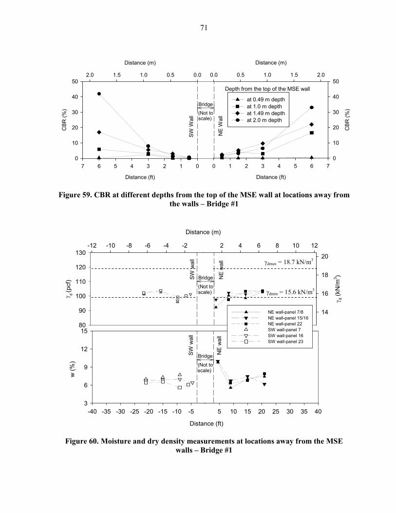
71

Figure 59. CBR at different depths from the top of the MSE wall at locations away from the walls – Bridge #1

Figure 60. Moisture and dry density measurements at locations away from the MSE walls – Bridge #1

Distance (ft)

01234567

CBR (%)

0

10

20

30

40

50

Distance (m)

0.00.51.01.52.0

at 0.49 m depthat 1.0 m depthat 1.49 m depthat 2.0 m depth

Distance (ft)

0 1 2 3 4 5 6 7

CBR (%)

0

10

20

30

40

50

Distance (m)

0.0 0.5 1.0 1.5 2.0

SW W

all

NE W

all

Bridge

(Not toscale)

Depth from the top of the MSE wall

γ d (pcf)

80

90

100

110

120

130

Distance (m)

-12 -10 -8 -6 -4 -2 0 2 4 6 8 10 12

γ d (kN

/m3 )

14

16

18

20

-40 -35 -30 -25 -20 -15 -10 -5 0 5 10 15 20 25 30 35 40

w (%)

3

6

9

12

15

NE wall-panel 7/8NE wall-panel 15/16NE wall-panel 22SW wall-panel 7SW wall-panel 16SW wall-panel 23

SW wall

NE wall

SW wall

NE wall

Bridge

(Not toscale)

Bridge

(Not toscale)

Distance (ft)

γdmax = 18.7 kN/m3

γdmin = 15.6 kN/m3

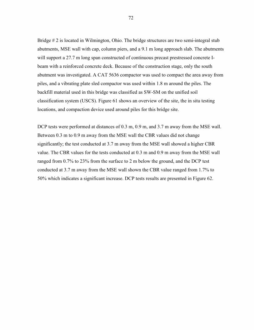
72

Bridge # 2 is located in Wilmington, Ohio. The bridge structures are two semi-integral stub

abutments, MSE wall with cap, column piers, and a 9.1 m long approach slab. The abutments

will support a 27.7 m long span constructed of continuous precast prestressed concrete I-

beam with a reinforced concrete deck. Because of the construction stage, only the south

abutment was investigated. A CAT 5636 compactor was used to compact the area away from

piles, and a vibrating plate sled compactor was used within 1.8 m around the piles. The

backfill material used in this bridge was classified as SW-SM on the unified soil

classification system (USCS). Figure 61 shows an overview of the site, the in situ testing

locations, and compaction device used around piles for this bridge site.

DCP tests were performed at distances of 0.3 m, 0.9 m, and 3.7 m away from the MSE wall.

Between 0.3 m to 0.9 m away from the MSE wall the CBR values did not change

significantly; the test conducted at 3.7 m away from the MSE wall showed a higher CBR

value. The CBR values for the tests conducted at 0.3 m and 0.9 m away from the MSE wall

ranged from 0.7% to 23% from the surface to 2 m below the ground, and the DCP test

conducted at 3.7 m away from the MSE wall shown the CBR value ranged from 1.7% to

50% which indicates a significant increase. DCP tests results are presented in Figure 62.

73

Figure 61. Bridge #2 at Wilmington: (a) overview of the south MSE wall; (b) DCP test locations; (c) vibratory plate compactor used to compaction of wall backfill

1’

3’

12’

(a)

(c)(b)

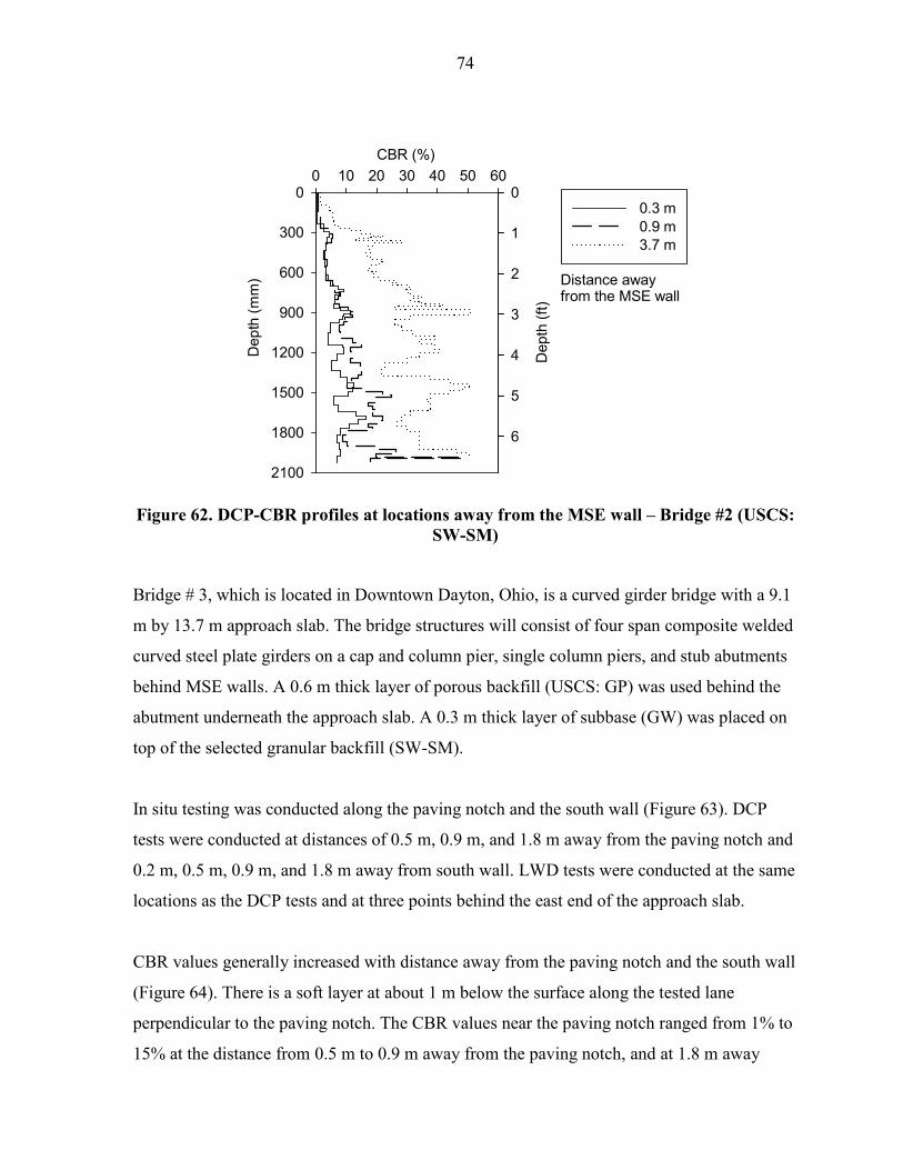
74

Figure 62. DCP-CBR profiles at locations away from the MSE wall – Bridge #2 (USCS: SW-SM)

Bridge # 3, which is located in Downtown Dayton, Ohio, is a curved girder bridge with a 9.1

m by 13.7 m approach slab. The bridge structures will consist of four span composite welded

curved steel plate girders on a cap and column pier, single column piers, and stub abutments

behind MSE walls. A 0.6 m thick layer of porous backfill (USCS: GP) was used behind the

abutment underneath the approach slab. A 0.3 m thick layer of subbase (GW) was placed on

top of the selected granular backfill (SW-SM).

In situ testing was conducted along the paving notch and the south wall (Figure 63). DCP

tests were conducted at distances of 0.5 m, 0.9 m, and 1.8 m away from the paving notch and

0.2 m, 0.5 m, 0.9 m, and 1.8 m away from south wall. LWD tests were conducted at the same

locations as the DCP tests and at three points behind the east end of the approach slab.

CBR values generally increased with distance away from the paving notch and the south wall

(Figure 64). There is a soft layer at about 1 m below the surface along the tested lane

perpendicular to the paving notch. The CBR values near the paving notch ranged from 1% to

15% at the distance from 0.5 m to 0.9 m away from the paving notch, and at 1.8 m away

CBR (%)0 10 20 30 40 50 60

Dep

th (mm)

0

300

600

900

1200

1500

1800

2100

Depth (ft)

0

1

2

3

4

5

6

0.3 m0.9 m3.7 m

Distance awayfrom the MSE wall

75

from the paving notch the CBR values ranged from 9% to 48%. The tests conducted along

the lane perpendicular to the south wall returned CBR values that range from 0.2% to 20%

within 0.9 m of the wall, and the CBR values for the test at 1.8 m away the wall ranged from

5% to 35%.

Figure 65 shows the LWD modulus change at test locations away from the paving notch and

the south wall. LWD tests were conducted at the same location as DCP tests in general, and

three tests were conducted at the location behind the end of approach slab. For these test

locations, the individual LWD modulus values ranged from 33 MPa to 72 MPa, and there

was no significant difference between the test locations with subbase or those without

subbase material. Figure 65 shows the modulus values with distance from the paving notch.

Figure 63. Bridge #3 (MOT-75-1393) at downtown Dayton

1.5’3’

6’

0.5’

1.5’

3’

6’

paving notch

South wall

In-situ testlocations

76

Figure 64. DCP-CBR profiles at locations away from south wall and paving notch at east abutment – Bridge #3

Figure 65. ELWD-Z2 measurements at locations away from paving notch and south wall on the east abutment – Bridge #3

Bridge # 4 is located at the Columbus, Ohio airport, near Johnstown Road. The bridge

structure is 18.8 m long, single span prestressed concrete I-beams with reinforced composite

deck on semi-integral abutments, which is supported by piles behind MSE walls. The

approach slabs were modified 9.1 m long section. Aggregate base (USCS: GP) was the

CBR (%)

0 10 20 30 40 50 60Depth (mm)

0

300

600

900

1200

1500

1800

2100

East abutmentPaving notch

CBR (%)

0 10 20 30 40 50 60

Depth (ft)

0

1

2

3

4

5

6

0.15 m - pea gravel0.46 m - subbase0.9 m - subbase1.83 m - subbase

East abutmentSouth wall

Distance away from paving notch / south wall

-40 -35 -30 -25 -20 -15 -10 -5 0

ELW

D-Z2 (M

Pa)

0

20

40

60

80

100

Distance (m)

-12 -10 -8 -6 -4 -2 0

Distance (ft)

0 5 10 15 20 25 30 35 40

ELW

D-Z2 (psi)

0

2500

5000

7500

10000

12500

0 2 4 6 8 10 12

Pea Gravel

Subbase

Pea Gravel

End

of A

pproach Slab

Subbase

Paving Notch

South W

all

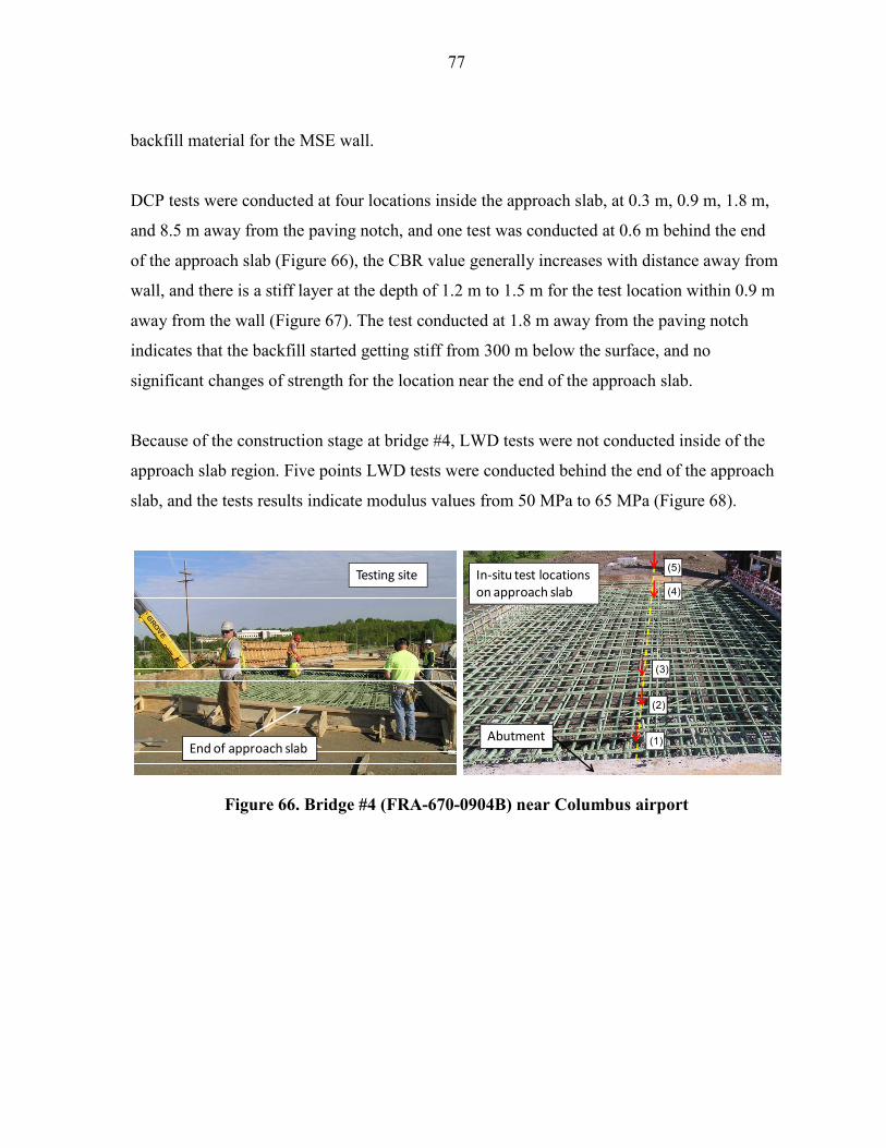
77

backfill material for the MSE wall.

DCP tests were conducted at four locations inside the approach slab, at 0.3 m, 0.9 m, 1.8 m,

and 8.5 m away from the paving notch, and one test was conducted at 0.6 m behind the end

of the approach slab (Figure 66), the CBR value generally increases with distance away from

wall, and there is a stiff layer at the depth of 1.2 m to 1.5 m for the test location within 0.9 m

away from the wall (Figure 67). The test conducted at 1.8 m away from the paving notch

indicates that the backfill started getting stiff from 300 m below the surface, and no

significant changes of strength for the location near the end of the approach slab.

Because of the construction stage at bridge #4, LWD tests were not conducted inside of the

approach slab region. Five points LWD tests were conducted behind the end of the approach

slab, and the tests results indicate modulus values from 50 MPa to 65 MPa (Figure 68).

Figure 66. Bridge #4 (FRA-670-0904B) near Columbus airport

Testing site In-situ test locationson approach slab

(1)

(5)

(4)

(3)

(2)

End of approach slabAbutment

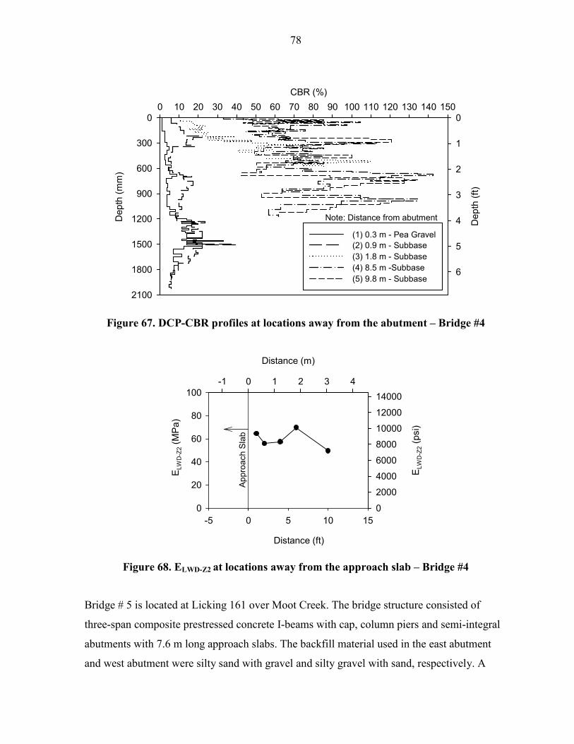
78

Figure 67. DCP-CBR profiles at locations away from the abutment – Bridge #4

Figure 68. ELWD-Z2 at locations away from the approach slab – Bridge #4

Bridge # 5 is located at Licking 161 over Moot Creek. The bridge structure consisted of

three-span composite prestressed concrete I-beams with cap, column piers and semi-integral

abutments with 7.6 m long approach slabs. The backfill material used in the east abutment

and west abutment were silty sand with gravel and silty gravel with sand, respectively. A

CBR (%)

0 10 20 30 40 50 60 70 80 90 100 110 120 130 140 150Depth (mm)

0

300

600

900

1200

1500

1800

2100

Depth (ft)

0

1

2

3

4

5

6

(1) 0.3 m - Pea Gravel(2) 0.9 m - Subbase(3) 1.8 m - Subbase(4) 8.5 m -Subbase(5) 9.8 m - Subbase

Note: Distance from abutment

Distance (m)

-1 0 1 2 3 4

ELW

D-Z2 (psi)

0

2000

4000

6000

8000

10000

12000

14000

-5 0 5 10 15

ELW

D-Z2 (M

Pa)

0

20

40

60

80

100

Distance (ft)

Approach Slab

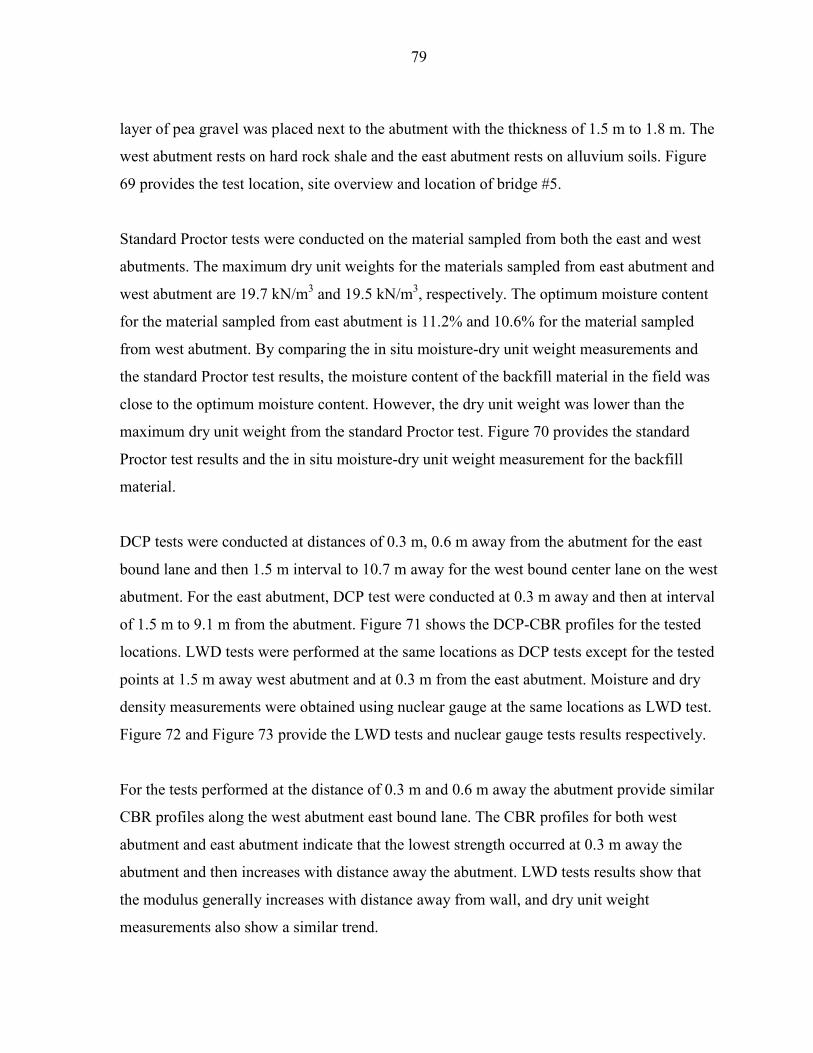
79

layer of pea gravel was placed next to the abutment with the thickness of 1.5 m to 1.8 m. The

west abutment rests on hard rock shale and the east abutment rests on alluvium soils. Figure

69 provides the test location, site overview and location of bridge #5.

Standard Proctor tests were conducted on the material sampled from both the east and west

abutments. The maximum dry unit weights for the materials sampled from east abutment and

west abutment are 19.7 kN/m3 and 19.5 kN/m3, respectively. The optimum moisture content

for the material sampled from east abutment is 11.2% and 10.6% for the material sampled

from west abutment. By comparing the in situ moisture-dry unit weight measurements and

the standard Proctor test results, the moisture content of the backfill material in the field was

close to the optimum moisture content. However, the dry unit weight was lower than the

maximum dry unit weight from the standard Proctor test. Figure 70 provides the standard

Proctor test results and the in situ moisture-dry unit weight measurement for the backfill

material.

DCP tests were conducted at distances of 0.3 m, 0.6 m away from the abutment for the east

bound lane and then 1.5 m interval to 10.7 m away for the west bound center lane on the west

abutment. For the east abutment, DCP test were conducted at 0.3 m away and then at interval

of 1.5 m to 9.1 m from the abutment. Figure 71 shows the DCP-CBR profiles for the tested

locations. LWD tests were performed at the same locations as DCP tests except for the tested

points at 1.5 m away west abutment and at 0.3 m from the east abutment. Moisture and dry

density measurements were obtained using nuclear gauge at the same locations as LWD test.

Figure 72 and Figure 73 provide the LWD tests and nuclear gauge tests results respectively.

For the tests performed at the distance of 0.3 m and 0.6 m away the abutment provide similar

CBR profiles along the west abutment east bound lane. The CBR profiles for both west

abutment and east abutment indicate that the lowest strength occurred at 0.3 m away the

abutment and then increases with distance away the abutment. LWD tests results show that

the modulus generally increases with distance away from wall, and dry unit weight

measurements also show a similar trend.

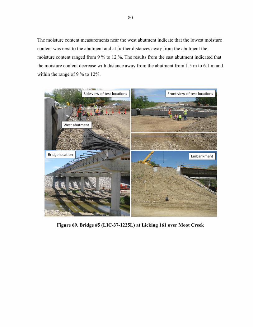
80

The moisture content measurements near the west abutment indicate that the lowest moisture

content was next to the abutment and at further distances away from the abutment the

moisture content ranged from 9 % to 12 %. The results from the east abutment indicated that

the moisture content decrease with distance away from the abutment from 1.5 m to 6.1 m and

within the range of 9 % to 12%.

Figure 69. Bridge #5 (LIC-37-1225L) at Licking 161 over Moot Creek

Side view of test locations Front view of test locations

Bridge location Embankment

West abutment

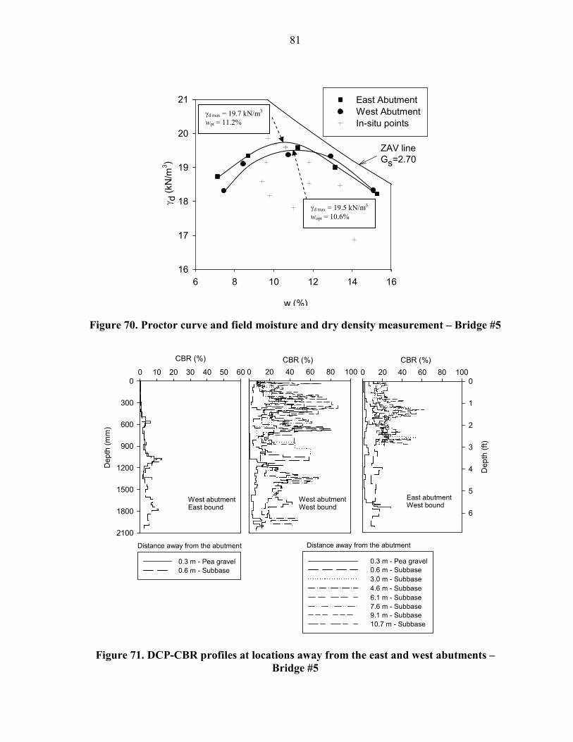
81

Figure 70. Proctor curve and field moisture and dry density measurement – Bridge #5

Figure 71. DCP-CBR profiles at locations away from the east and west abutments – Bridge #5

w (%)

6 8 10 12 14 16

γ d (kN

/m3 )

16

17

18

19

20

21 East AbutmentWest AbutmentIn-situ points

ZAV lineGs=2.70

CBR (%)

0 20 40 60 80 100

Dep

th (ft)

0

1

2

3

4

5

6

CBR (%)

0 20 40 60 80 100

0.3 m - Pea gravel0.6 m - Subbase3.0 m - Subbase4.6 m - Subbase6.1 m - Subbase7.6 m - Subbase9.1 m - Subbase10.7 m - Subbase

CBR (%)

0 10 20 30 40 50 60

Dep

th (mm)

0

300

600

900

1200

1500

1800

2100

0.3 m - Pea gravel0.6 m - Subbase

West abutmentEast bound

West abutmentWest bound

East abutmentWest bound

Distance away from the abutmentDistance away from the abutment

γd max = 19.5 kN/m3 wopt = 10.6%

γd max = 19.7 kN/m3 wpt = 11.2%

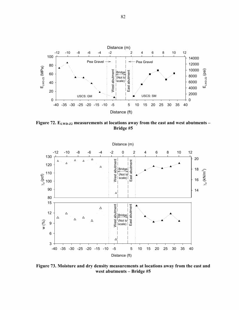
82

Figure 72. ELWD-Z2 measurements at locations away from the east and west abutments – Bridge #5

Figure 73. Moisture and dry density measurements at locations away from the east and west abutments – Bridge #5

-40 -35 -30 -25 -20 -15 -10 -5 0 5 10 15 20 25 30 35 40

ELW

D-Z2 ( M

Pa)

0

20

40

60

80

100

Distance (m)-12 -10 -8 -6 -4 -2 0 2 4 6 8 10 12

ELW

D-Z2 (psi)

0

2000

4000

6000

8000

10000

12000

14000

West abutm

ent

East abutm

ent

Bridge

(Not toscale)

Distance (ft)

Pea Gravel Pea Gravel

USCS: GM USCS: SM

Distance (m)

-12 -10 -8 -6 -4 -2 0 2 4 6 8 10 12

γ d (kN

/m3 )

14

16

18

20

γ d (pcf)

80

90

100

110

120

130

-40 -35 -30 -25 -20 -15 -10 -5 0 5 10 15 20 25 30 35 40

w (%)

3

6

9

12

15

West abutm

ent

East abu

tmen

t

West abu

tment

East abutm

ent

Bridge

(Not toscale)

Bridge

(Not toscale)

Distance (ft)

83

Bridge # 6 located at the interchange of I-71 & I-76 on the section of I-71 over Greenwich

Road at Medina County, Ohio. The structures for this project site was a single span steel

girder bridge with reinforced concrete deck and semi-integral wall type abutments with a 9.1

m long modified approach slab. There was an existing wall about 9.1 m away from the new

wall. A gap between the existing slab and the exposed fill material can be seen from the

existing wall. Figure 74 shows the project site conditions and in situ tests locations for this

bridge study and the conducted in situ tests include DCP, LWD and PLT along two testing

lanes. The material from the site is classified as poorly graded gravel to silty gravel with sand

per USCS.

DCP tests were conducted on two testing lanes which were west lane and east lane at 0.3 m

away from the abutment and then at 1.5 m interval to 9.1 m from the abutment. Figure 75

provides the DCP tests results in terms of CBR values for both west and east lanes. The CBR

profiles from the west lane shows that at the same depth CBR values increase with distance

away from wall, but with the distance of 7.6 m to 9.1 m away from the wall the CBR values

start to decrease. That may caused by the existing wall near the end of the west lane. The

DCP tests conducted on the east lane also gives the similar conclusion.

LWD tests were performed on both east and west testing lanes along south abutment. Nine

testing points were constructed on east testing lane and thirteen points were tested along west

lane on south abutment. Figure 76 shows the ELWD-Z2 varies with distance away from the

south abutment for both testing lanes. The LWD tests results indicated that the modulus

values at the middle part of the two testing lanes are higher than the ELWD measured at the

ends, and the modulus values from the two testing lanes show similar trend and the typical

ELWD-Z2 range was 5 MPa to 30 MPa.

PLTs were conducted at three locations that parallel the new abutment within a distance of

4.9 m away from the abutment. At the third testing point, water was introduced at the surface

of the soil while maintaining a static stress of 0.4 MPa to evaluate the collapse potential of

the backfill material. Figure 77 provides the PLTs results and the test setup. The PLT

84

indicates minimal in situ collapse potential, because only 8 mm additional settlement was

shown up when the material was saturated and that was less than the settlement during the

loading stage.

Figure 74. Bridge #6 (MED-71-0729) at I-71 and I-76 interchange: (a) location of test site; (b) void under the existing slab and old backfill material (c) in situ test locations –

east lane (d) in situ test locations – west lane

Existing wall

Existing slab

Old backfill material

Void under the slab

(a) (b)

(c) (d)

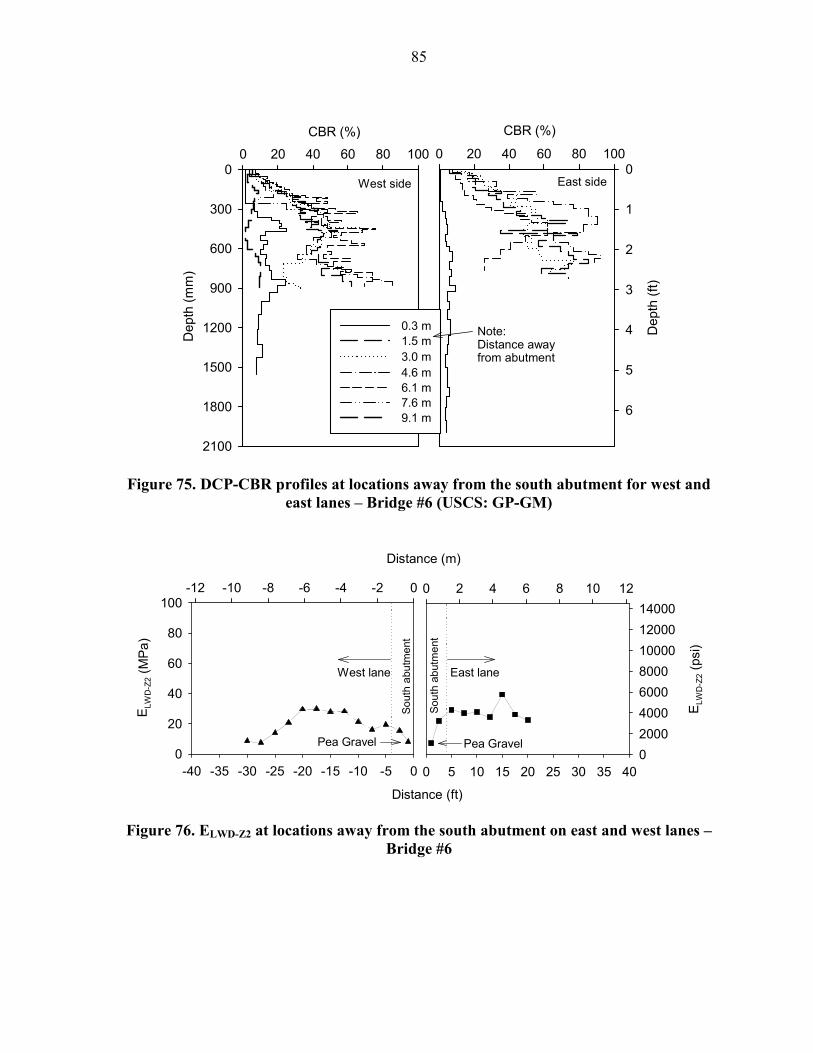
85

Figure 75. DCP-CBR profiles at locations away from the south abutment for west and east lanes – Bridge #6 (USCS: GP-GM)

Figure 76. ELWD-Z2 at locations away from the south abutment on east and west lanes – Bridge #6

CBR (%)

0 20 40 60 80 100

Depth (ft)

0

1

2

3

4

5

6

CBR (%)

0 20 40 60 80 100

Depth (mm)

0

300

600

900

1200

1500

1800

2100

0.3 m1.5 m3.0 m4.6 m6.1 m7.6 m9.1 m

West side East side

Note:Distance awayfrom abutment

-40 -35 -30 -25 -20 -15 -10 -5 0

ELW

D-Z2 (M

Pa)

0

20

40

60

80

100

Distance (m)

-12 -10 -8 -6 -4 -2 0

Sou

th abu

tmen

t

Distance (ft)

0 5 10 15 20 25 30 35 40

ELW

D-Z2 (psi)

0

2000

4000

6000

8000

10000

12000

14000

0 2 4 6 8 10 12

Sou

th abu

tmen

t

Pea Gravel Pea Gravel

East laneWest lane

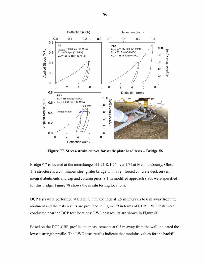
86

Figure 77. Stress-strain curves for static plate load tests – Bridge #6

Bridge # 7 is located at the interchange of I-71 & I-76 over I-71 at Medina County, Ohio.

The structure is a continuous steel girder bridge with a reinforced concrete deck on semi-

integral abutments and cap and column piers. 9.1 m modified approach slabs were specified

for this bridge. Figure 78 shows the in situ testing locations.

DCP tests were performed at 0.2 m, 0.3 m and then at 1.5 m intervals to 6 m away from the

abutment and the tests results are provided in Figure 79 in terms of CBR. LWD tests were

conducted near the DCP test locations; LWD test results are shown in Figure 80.

Based on the DCP-CBR profile, the measurements at 0.3 m away from the wall indicated the

lowest strength profile. The LWD tests results indicate that modulus values for the backfill

PT1

0 2 4 6 8

Applied Stress (M

Pa)

0.0

0.2

0.4

0.6

0.8

Deflection (inch)

0.0 0.1 0.2 0.3

PT2

Deflection (mm)

0 2 4 6 8

Deflection (inch)

0.0 0.1 0.2 0.3

Applied Stress (psi)

0

20

40

60

80

100

PT3

Deflection (mm)

0 2 4 6 8

Applied Stress (M

Pa)

0.0

0.2

0.4

0.6

0.8

App

lied Stress (psi)

0

20

40

60

80

100

ELWD-Z2 = 5076 psi (35 MPa)EV1= 4685 psi (32 MPa)EV2= 16810 psi (116 MPa)

ELWD-Z2 = 4424 psi (31 MPa)EV1= 5018 psi (35 MPa)EV2= 13822 psi (95 MPa)

Added Water

~ 0.8 mm

EV1= 5555 psi (38 MPa)EV2= 16244 psi (112 MPa)

PT 3

87

ranged from 5 MPa to 35 MPa.

Figure 78. Bridge #7 (MED-71-0750) at I-71 and I-76 interchange: (a) site location; (b) in situ test locations

Figure 79. DCP-CBR profiles at locations away from east abutment – Bridge #7

Existing wall

5’

5’

5’4’

0.5’

(a) (b)

CBR (%)

0 20 40 60 80 100

Depth (mm)

0

300

600

900

1200

1500

1800

2100

Depth (ft)

0

1

2

3

4

5

6

0.15 m0.3 m1.5 m3.0 m4.6 m6.1 m

East abutment

Note: Distance from abutment

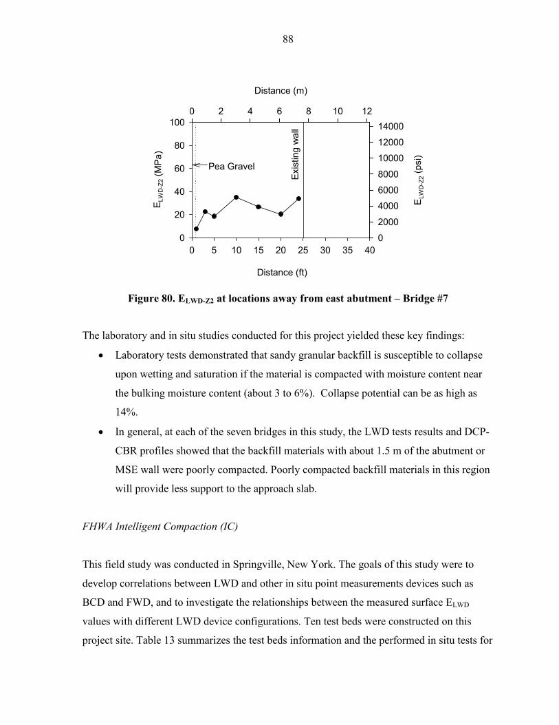
88

Figure 80. ELWD-Z2 at locations away from east abutment – Bridge #7

The laboratory and in situ studies conducted for this project yielded these key findings:

• Laboratory tests demonstrated that sandy granular backfill is susceptible to collapse

upon wetting and saturation if the material is compacted with moisture content near

the bulking moisture content (about 3 to 6%). Collapse potential can be as high as

14%.

• In general, at each of the seven bridges in this study, the LWD tests results and DCP-

CBR profiles showed that the backfill materials with about 1.5 m of the abutment or

MSE wall were poorly compacted. Poorly compacted backfill materials in this region

will provide less support to the approach slab.

FHWA Intelligent Compaction (IC)

This field study was conducted in Springville, New York. The goals of this study were to

develop correlations between LWD and other in situ point measurements devices such as

BCD and FWD, and to investigate the relationships between the measured surface ELWD

values with different LWD device configurations. Ten test beds were constructed on this

project site. Table 13 summarizes the test beds information and the performed in situ tests for

0 5 10 15 20 25 30 35 40

ELW

D-Z2 (M

Pa)

0

20

40

60

80

100

Distance (m)

0 2 4 6 8 10 12

ELW

D-Z2 (psi)

0

2000

4000

6000

8000

10000

12000

14000

Distance (ft)

Pea Gravel

Existing wall

89

each test bed.

Table 13. Summary of test beds and performed in situ testing

TB Material Test bed Structure Test bed Size In situ Test

1 Embankment A section of rubber tire fill at < 1 m below the grade 18 m × 200 m DCP, LWD

2 Embankment A section of rubber tire fill at < 1 m below the grade 18 m × 71 m DCP, LWD

3 Embankment Compacted embankment granular subgrade material 10 m × 105 m LWD

4 Gravel

Subbase

2 m to 2.5 m thick loosely placed aggregate subbase material over geofabric placed on top of TBs 1

and 2

―* BCD, LWD

5 ―* BCD, DCP, LWD

6 Gravel Subbase

Aggregate subbase material placed over geofabric on top of TB1

embankment material

―* DCP, LWD, BCD 7 ―*

8 Embankment Compacted embankment granular subgrade material 10 m × 100 m FWD, PLT

9 Gravel Subbase

Aggregate subbase material placed over geofabric on top of a

compacted embankment layer ―* BCD, LWD,

DCP

10 Embankment Compacted embankment granular subgrade material ―* BCD, DCP,

LWD, PLT

Note: * not measured

To avoid the relative influence and sensitivity of soil disturbance on test results, the tests

were performed in the following order: FWD, LWD, BCD, and DCP. The LWD drop height

of the LWD apparatus was adjusted to obtain the same applied contact stress for each of the

200 mm, 150 mm and 100 mm diameter plates. The measured ELWD values on test bed 2 are

provided in Table 14.

The key findings from this field case study are provided in the correlation evaluation

sections.

90

Table 14. Field LWD measurements from FHWA New York site

Applied stress

Device configuration Point # 1 2 3 4 5 6

σo= 190 N/m2

D=200 mm ELWD, MPa 92.42 146.60 69.32 37.51 177.14 67.84

h=50 cm D=150 mm ELWD,

MPa 37.07 116.60 47.50 19.61 54.81 32.39 h=16 cm

D=100 mm ELWD, MPa 43.21 176.43 66.86 26.91 94.80 23.01 h=3.1 cm

σo= 230 N/m2

D=200 mm ELWD, MPa 126.49 263.88 103.41 38.45 168.18 66.25

h=72 cm D=150 mm ELWD,

MPa 75.05 197.99 85.70 32.90 73.14 52.92 h=22.8 cm D=100 mm ELWD,

MPa 57.11 231.89 85.98 28.66 115.95 30.13 h=4.5 cm

σo= 340 N/m2

D=150 mm ELWD, MPa 91.43 327.03 85.89 35.58 85.03 61.61 h=50 cm

D=100 mm ELWD, MPa 65.17 246.50 90.71 34.78 87.90 49.95

h=9.9 cm

σo= 400 N/m2

D=150 mm ELWD, MPa 61.46 329.13 97.17 42.25 87.21 56.84

h=72 cm D=100 mm ELWD,

MPa 70.07 256.48 82.89 33.07 97.10 42.09 h=14.2 cm

Pavement Foundation Study

The pavement foundation study was conducted on two sections along I-94 in St. Clair and

Macomb Counties, Michigan. The two goals of this study were to obtain typical elastic

modulus values for different field conditions by performing LWD tests, and to obtain the

correlations between LWD measurements and FWD measurements. Three test beds were

identified for this study. Test bed 1 consisted of 40.6 cm of compacted and trimmed open-

graded aggregate subbase material over a recompacted mixture of sand and silty clays soils.

A 6.1 m by 6.1 m grid was built on this test bed to perform LWD, DCP, and NG tests and the

test points were set on 0.61 m centers Figure 81.

Test bed 2 was a 23 cm thick existing concrete pavement which was built 40 years ago as

shown in Figure 82. FWD tests were performed before the panels were removed, then the

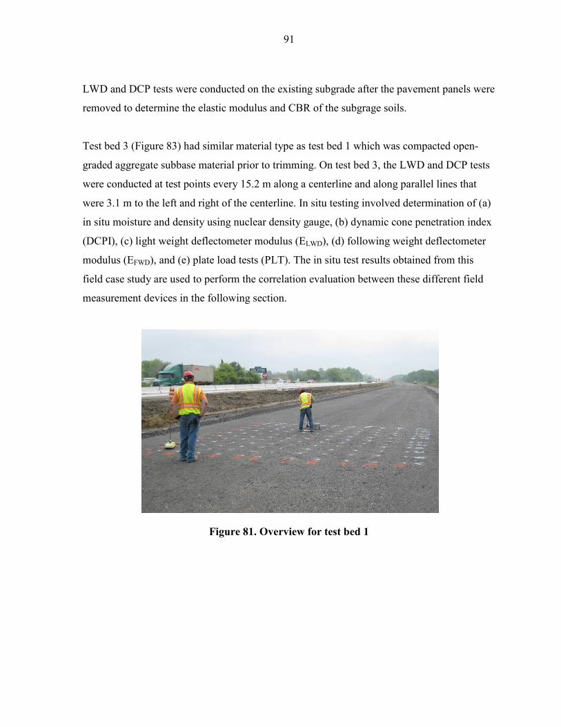
91

LWD and DCP tests were conducted on the existing subgrade after the pavement panels were

removed to determine the elastic modulus and CBR of the subgrage soils.

Test bed 3 (Figure 83) had similar material type as test bed 1 which was compacted open-

graded aggregate subbase material prior to trimming. On test bed 3, the LWD and DCP tests

were conducted at test points every 15.2 m along a centerline and along parallel lines that

were 3.1 m to the left and right of the centerline. In situ testing involved determination of (a)

in situ moisture and density using nuclear density gauge, (b) dynamic cone penetration index

(DCPI), (c) light weight deflectometer modulus (ELWD), (d) following weight deflectometer

modulus (EFWD), and (e) plate load tests (PLT). The in situ test results obtained from this

field case study are used to perform the correlation evaluation between these different field

measurement devices in the following section.

Figure 81. Overview for test bed 1

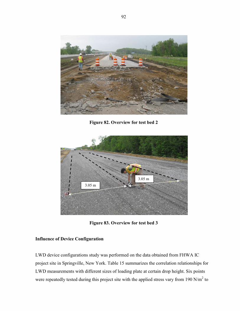
92

Figure 82. Overview for test bed 2

Figure 83. Overview for test bed 3

Influence of Device Configuration

LWD device configurations study was performed on the data obtained from FHWA IC

project site in Springville, New York. Table 15 summarizes the correlation relationships for

LWD measurements with different sizes of loading plate at certain drop height. Six points

were repeatedly tested during this project site with the applied stress vary from 190 N/m2 to

3.05 m

3.05 m

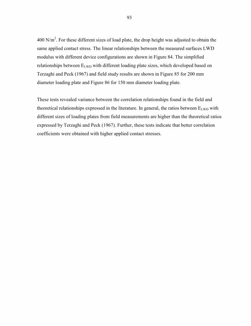
93

400 N/m2. For these different sizes of load plate, the drop height was adjusted to obtain the

same applied contact stress. The linear relationships between the measured surfaces LWD

modulus with different device configurations are shown in Figure 84. The simplified

relationships between ELWD with different loading plate sizes, which developed based on

Terzaghi and Peck (1967) and field study results are shown in Figure 85 for 200 mm

diameter loading plate and Figure 86 for 150 mm diameter loading plate.

These tests revealed variance between the correlation relationships found in the field and

theoretical relationships expressed in the literature. In general, the ratios between ELWD with

different sizes of loading plates from field measurements are higher than the theoretical ratios

expressed by Terzaghi and Peck (1967). Further, these tests indicate that better correlation

coefficients were obtained with higher applied contact stresses.

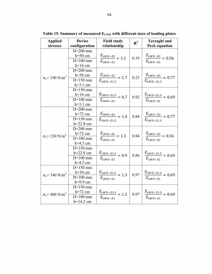
94

Table 15. Summary of measured ELWD with different sizes of loading plates

Applied stresses

Device configuration

Field study relationship R2 Terzaghi and

Peck equation

σo= 190 N/m2

D=200 mm h=50 cm �T ��U�T ��U� � %"% 0.19

�T ��U�T ��U� � ,"+# D=100 mm h=16 cm

D=200 mm h=50 cm �T ��U�T ��U�"- � %"& 0.23

�T ��U�T ��U�"- � ,"&& D=150 mm h=3.1 cm

D=150 mm h=16 cm �T ��U�"-�T ��U� � ,"& 0.92

�T ��U�"-�T ��U� � ,"#2 D=100 mm h=3.1 cm

σo= 230 N/m2

D=200 mm h=72 cm �T ��U�T ��U�"- � %"1 0.84

�T ��U�T ��U�"- � ,"&& D=150 mm h=22.8 cm D=200 mm

h=72 cm �T ��U�T ��U� � %"V 0.84 �T ��U�T ��U� � ,"+# D=100 mm

h=4.5 cm D=150 mm h=22.8 cm �T ��U�"-�T ��U� � ,"2 0.86

�T ��U�"-�T ��U� � ,"#2 D=100 mm h=4.5 cm

σo= 340 N/m2

D=150 mm h=50 cm �T ��U�"-�T ��U� � %"V 0.97

�T ��U�"-�T ��U� � ,"#2 D=100 mm h=9.9 cm

σo= 400 N/m2

D=150 mm h=72 cm �T ��U�"-�T ��U� � %"! 0.97

�T ��U�"-�T ��U� � ,"#2 D=100 mm h=14.2 cm

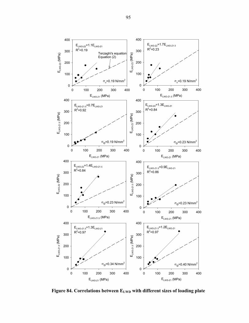
95

Figure 84. Correlations between ELWD with different sizes of loading plate

σo=0.19 N/mm2

ELWD-Z1 (MPa)

0 100 200 300 400

ELW

D-Z2 (M

Pa)

0

100

200

300

400

σo=0.23 N/mm2

ELWD-Z1 (MPa)

0 100 200 300 400

ELW

D-Z2 (M

Pa)

0

100

200

300

400

σo=0.19 N/mm2

ELWD-Z1.5 (MPa)

0 100 200 300 400

ELW

D-Z2 (M

Pa)

0

100

200

300

400

σo=0.19 N/mm2

ELWD-Z1 (MPa)

0 100 200 300 400

ELW

D-Z1.5 (M

Pa)

0

100

200

300

400

σo=0.23 N/mm2

ELWD-Z1.5 (MPa)

0 100 200 300 400

ELW

D-Z2 (M

Pa)

0

100

200

300

400

σo=0.23 N/mm2

ELWD-Z1 (MPa)

0 100 200 300 400

ELW

D-Z1.5 (M

Pa)

0

100

200

300

400

σo=0.34 N/mm2

ELWD-Z1 (MPa)

0 100 200 300 400

ELW

D-Z1.5 (M

Pa)

0

100

200

300

400

σo=0.40 N/mm2

ELWD-Z1 (MPa)

0 100 200 300 400

ELW

D-Z1.5 (M

Pa)

0

100

200

300

400

ELWD-Z2=1.1ELWD-Z1

R2=0.19

ELWD-Z2=1.7ELWD-Z1.5

R2=0.23

ELWD-Z1.5=0.7ELWD-Z1

R2=0.92

ELWD-Z2=1.3ELWD-Z1

R2=0.84

ELWD-Z2=1.4ELWD-Z1.5

R2=0.84ELWD-Z1.5=0.9ELWD-Z1

R2=0.86

ELWD-Z1.5=1.3ELWD-Z1

R2=0.97

ELWD-Z1.5=1.2ELWD-Z1

R2=0.97

Terzaghi's equationEquation (2)

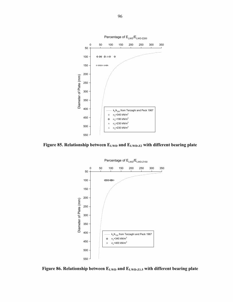
96

Figure 85. Relationship between ELWD and ELWD-Z2 with different bearing plate

Figure 86. Relationship between ELWD and ELWD-Z1.5 with different bearing plate

Percentage of ELWD/ELWD-Z200

0 50 100 150 200 250 300 350

Diameter of P

late (mm)

50

100

150

200

250

300

350

400

450

500

550

ks/k200 from Terzaghi and Peck 1967

σo=340 kN/m2

σo=190 kN/m2

σo=230 kN/m2

σo=230 kN/m2

Percentage of ELWD/ELWD-Z150

0 50 100 150 200 250 300 350

Diameter of P

late (mm)

50

100

150

200

250

300

350

400

450

500

550

ks/k150 from Terzaghi and Peck 1967

σo=340 kN/m2

σo=400 kN/m2

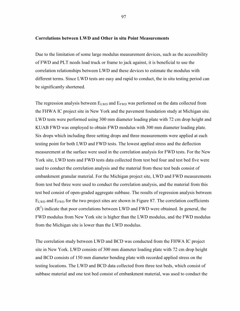
97

Correlations between LWD and Other in situ Point Measurements

Due to the limitation of some large modulus measurement devices, such as the accessibility

of FWD and PLT needs load truck or frame to jack against, it is beneficial to use the

correlation relationships between LWD and these devices to estimate the modulus with

different terms. Since LWD tests are easy and rapid to conduct, the in situ testing period can

be significantly shortened.

The regression analysis between ELWD and EFWD was performed on the data collected from

the FHWA IC project site in New York and the pavement foundation study at Michigan site.

LWD tests were performed using 300 mm diameter loading plate with 72 cm drop height and

KUAB FWD was employed to obtain FWD modulus with 300 mm diameter loading plate.

Six drops which including three setting drops and three measurements were applied at each

testing point for both LWD and FWD tests. The lowest applied stress and the deflection

measurement at the surface were used in the correlation analysis for FWD tests. For the New

York site, LWD tests and FWD tests data collected from test bed four and test bed five were

used to conduct the correlation analysis and the material from these test beds consist of

embankment granular material. For the Michigan project site, LWD and FWD measurements

from test bed three were used to conduct the correlation analysis, and the material from this

test bed consist of open-graded aggregate subbase. The results of regression analysis between

ELWD and EFWD for the two project sites are shown in Figure 87. The correlation coefficients

(R2) indicate that poor correlations between LWD and FWD were obtained. In general, the

FWD modulus from New York site is higher than the LWD modulus, and the FWD modulus

from the Michigan site is lower than the LWD modulus.

The correlation study between LWD and BCD was conducted from the FHWA IC project

site in New York. LWD consists of 300 mm diameter loading plate with 72 cm drop height

and BCD consists of 150 mm diameter bending plate with recorded applied stress on the

testing locations. The LWD and BCD data collected from three test beds, which consist of

subbase material and one test bed consist of embankment material, was used to conduct the

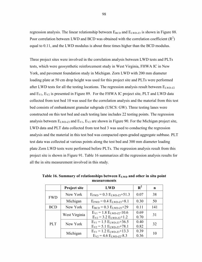
98

regression analysis. The linear relationship between EBCD and ELWD-Z3 is shown in Figure 88.

Poor correlation between LWD and BCD was obtained with the correlation coefficient (R2)

equal to 0.11, and the LWD modulus is about three times higher than the BCD modulus.

Three project sites were involved in the correlation analysis between LWD tests and PLTs

tests, which were geosynthetic reinforcement study in West Virginia, FHWA IC in New

York, and pavement foundation study in Michigan. Zorn LWD with 200 mm diameter

loading plate at 50 cm drop height was used for this project site and PLTs were performed

after LWD tests for all the testing locations. The regression analysis result between ELWD-Z2

and EV1, EV2 is presented in Figure 89. For the FHWA IC project site, PLT and LWD data

collected from test bed 10 was used for the correlation analysis and the material from this test

bed consists of embankment granular subgrade (USCS: GW). Three testing lanes were

constructed on this test bed and each testing lane includes 22 testing points. The regression

analysis between ELWD-Z3 and EV1, EV2 are shown in Figure 90. For the Michigan project site,

LWD data and PLT data collected from test bed 3 was used to conducting the regression

analysis and the material in this test bed was compacted open-graded aggregate subbase. PLT

test data was collected at various points along the test bed and 300 mm diameter loading

plate Zorn LWD tests were performed before PLTs. The regression analysis result from this

project site is shown in Figure 91. Table 16 summarizes all the regression analysis results for

all the in situ measurement involved in this study.

Table 16. Summary of relationships between ELWD and other in situ point measurements

Project site LWD R2 n

FWD New York EFWD = 0.3 ELWD-Z3+51.3 0.07 38

Michigan EFWD = 0.4 ELWD-Z3+8.1 0.30 50

BCD New York EBCD = 0.3 ELWD-Z3+29 0.11 141

PLT

West Virginia EV1 = 1.8 ELWD-Z2-10.6 EV2 = 3.2 ELWD-Z2+1.2

0.69 0.70 31

New York EV1 = 1.5 ELWD-Z3+36.5 EV2 = 5.1 ELWD-Z3+78.1

0.40 0.82 32

Michigan EV1 = 1.2 ELWD-Z3+13.3 EV2 = 4.6 ELWD-Z2-8.3

0.39 0.36 10

99

Figure 87. Correlations between ELWD and EFWD with 300 mm diameter loading plate

Figure 88. Correlation between LWD measurement and BCD measurements

ELWD-Z3 (MPa)

0 100 200 300 400 500

EFW

D (MPa)

0

100

200

300

400

500

New York SiteMichigan Site

EFWD-D3=1.7 ELWD-Z3+66.2

R2=0.63

EFWD-D3=0.8 ELWD-Z3+16.2

R2=0.30

ELWD-Z3 (MPa)

0 20 40 60 80 100 120 140

EBCD (MPa)

0

20

40

60

80

100

120

140

EBCD = 0.3ELWD-Z3+29

R2=0.11

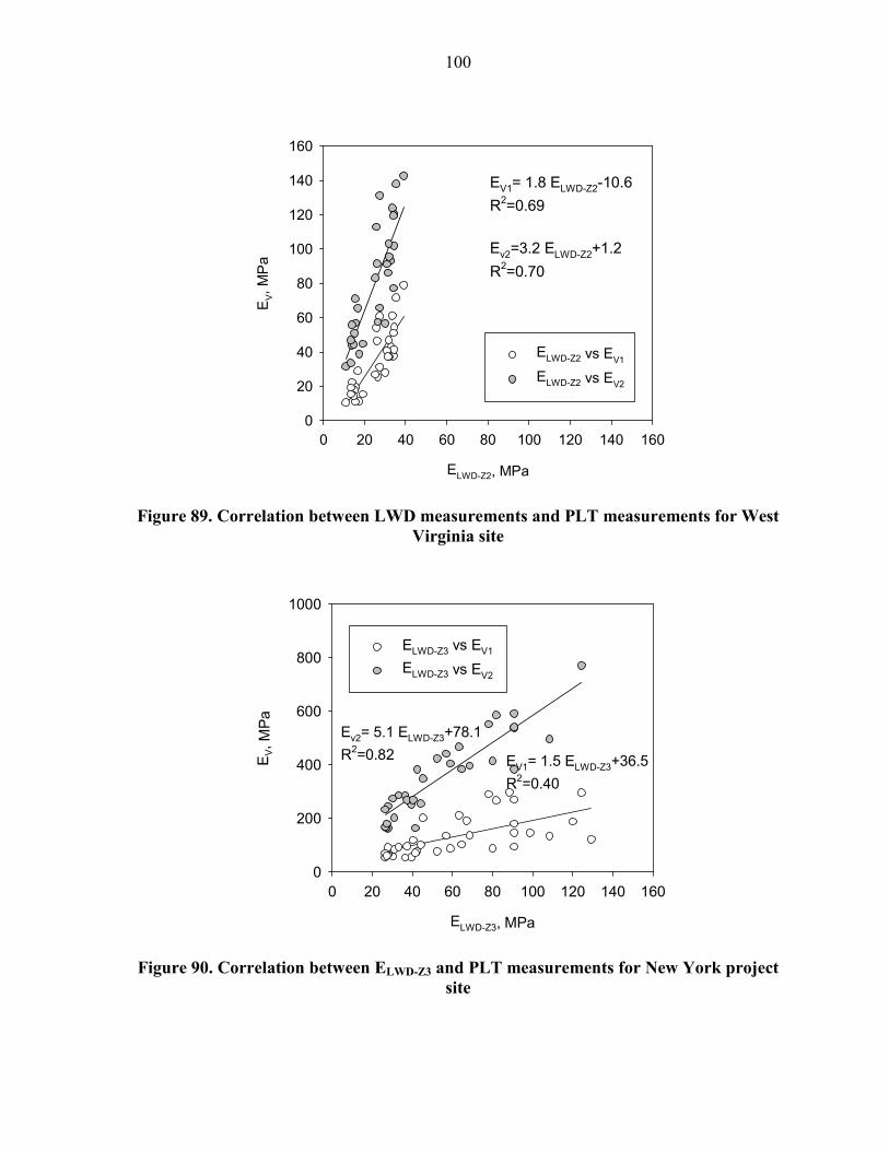
100

Figure 89. Correlation between LWD measurements and PLT measurements for West Virginia site

Figure 90. Correlation between ELWD-Z3 and PLT measurements for New York project site

ELWD-Z2, MPa

0 20 40 60 80 100 120 140 160

EV, M

Pa

0

20

40

60

80

100

120

140

160

ELWD-Z2 vs EV1

ELWD-Z2 vs EV2

EV1= 1.8 ELWD-Z2-10.6

R2=0.69

Ev2=3.2 ELWD-Z2+1.2

R2=0.70

EV1= 1.5 ELWD-Z3+36.5

R2=0.40

ELWD-Z3, MPa

0 20 40 60 80 100 120 140 160

EV, M

Pa

0

200

400

600

800

1000

ELWD-Z3 vs EV1

ELWD-Z3 vs EV2

Ev2= 5.1 ELWD-Z3+78.1

R2=0.82

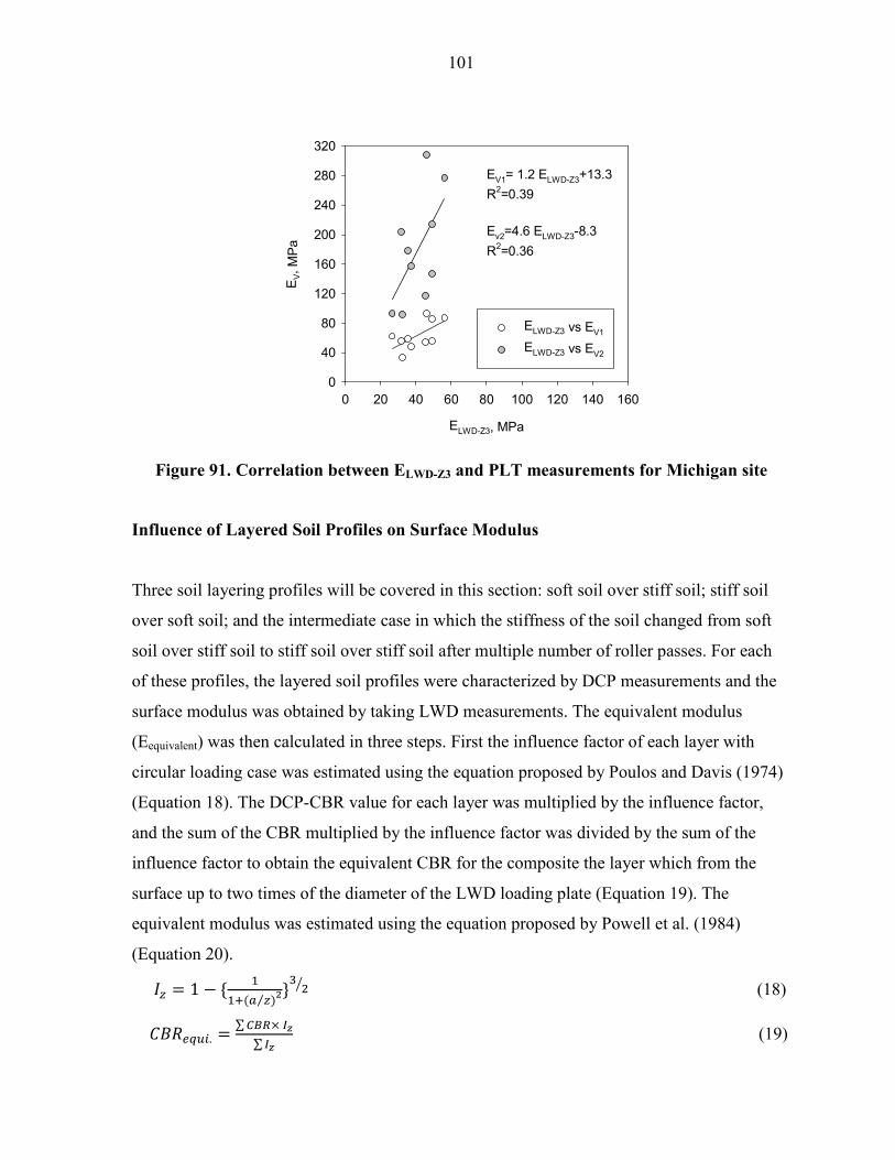
101

Figure 91. Correlation between ELWD-Z3 and PLT measurements for Michigan site

Influence of Layered Soil Profiles on Surface Modulus

Three soil layering profiles will be covered in this section: soft soil over stiff soil; stiff soil

over soft soil; and the intermediate case in which the stiffness of the soil changed from soft

soil over stiff soil to stiff soil over stiff soil after multiple number of roller passes. For each

of these profiles, the layered soil profiles were characterized by DCP measurements and the

surface modulus was obtained by taking LWD measurements. The equivalent modulus

(Eequivalent) was then calculated in three steps. First the influence factor of each layer with

circular loading case was estimated using the equation proposed by Poulos and Davis (1974)

(Equation 18). The DCP-CBR value for each layer was multiplied by the influence factor,

and the sum of the CBR multiplied by the influence factor was divided by the sum of the

influence factor to obtain the equivalent CBR for the composite the layer which from the

surface up to two times of the diameter of the LWD loading plate (Equation 19). The

equivalent modulus was estimated using the equation proposed by Powell et al. (1984)

(Equation 20).

*4 � % $ W ���P 4�3 �X: Y (18)

�� MZ[�" � \E�L@�F8\ F8 (19)

EV1= 1.2 ELWD-Z3+13.3

R2=0.39

Ev2=4.6 ELWD-Z3-8.3

R2=0.36

ELWD-Z3, MPa

0 20 40 60 80 100 120 140 160

EV, M

Pa

0

40

80

120

160

200

240

280

320

ELWD-Z3 vs EV1

ELWD-Z3 vs EV2

102

�MZ[��P]M^_�`)a� � %&"+b @ cdefghi"G"jk (20)

A sample calculation for estimating the equivalent modulus using DCP measurements is

shown in Figure 92.

The first set of data was collected from Ohio bridge approach project site and 31 testing

points were evaluated. The data can be separated into two groups, which collected further

than 6 m away the abutment and collected within 6 m from abutment. Data collected from 6

m away the abutment was the case of stiff soil over soft soil and data collected within 6 m

away the abutment was the case of soft soil over stiff soil. Good correlation coefficients (R2

= 0.72) were obtained from both cases as shown in Figure 93 and the calculations for all data

points are provided in Appendix.

Figure 92. Sample calculation for estimating the equivalent modulus using DCP measurements

CBR (%)

5 10 15 20 25

Dep

th (mm)

0

50

100

150

200

250

300

350

400

Iz

0.0 0.2 0.4 0.6 0.8 1.0(1)

PT # Depth (mm) CBR IZ CBR××××IZ

1 0 12.6 1.0 23.12 33 12.6 1.0 12.33 183 17.3 0.3 5.64 277 23.7 0.2 4.05 395 14.3 0.1 1.3

Sum (CBR×IZ): 23.1

Sum (IZ): 1.6

CBRequi. = Sum (CBR×IZ)/sum(IZ) 14.9

Eequi.= 17.6×CBRequi.0.64 99.1

(1)

(2)

(3)

(4)

(5)

(2)

(3)

(4)

(5)

103

Figure 93. Correlation between Eequivalent and ELWD-Z2 for Ohio project site

The second profile, stiff soil over soft soil, was found at the Hormel PCC project site, and 84

points were tested. The regression analysis result (R2 = 0.54) from this project site provides a

better correlation than the case of soft soil over stiff soil (Figure 94), and the calculations for

all data points are provided in Appendix.

Figure 94. Correlation between Eequivalent and ELWD-Z2 for Hormel PCC project site

Eequivalent (MPa)

0 50 100 150 200

ELW

D-Z2 (M

Pa)

0

20

40

60

80

100CBR (%)

0 5 10 15 20 25 30

Depth (mm)

0

50

100

150

200

250

300

350

400

ELWD-Z2 = 3.2 Eequi. + 25.7

R2 = 0.72, n = 22

ELWD-Z2 = 2.3 Eequi. - 21.4

R2 = 0.72, n = 9

Eequivalent (MPa)

0 50 100 150 200 250

ELW

D-Z2 (M

Pa)

0

20

40

60

80

100ELWD-Z2 = 0.2 Eequivalent - 4.2

R2 = 0.54, n = 84

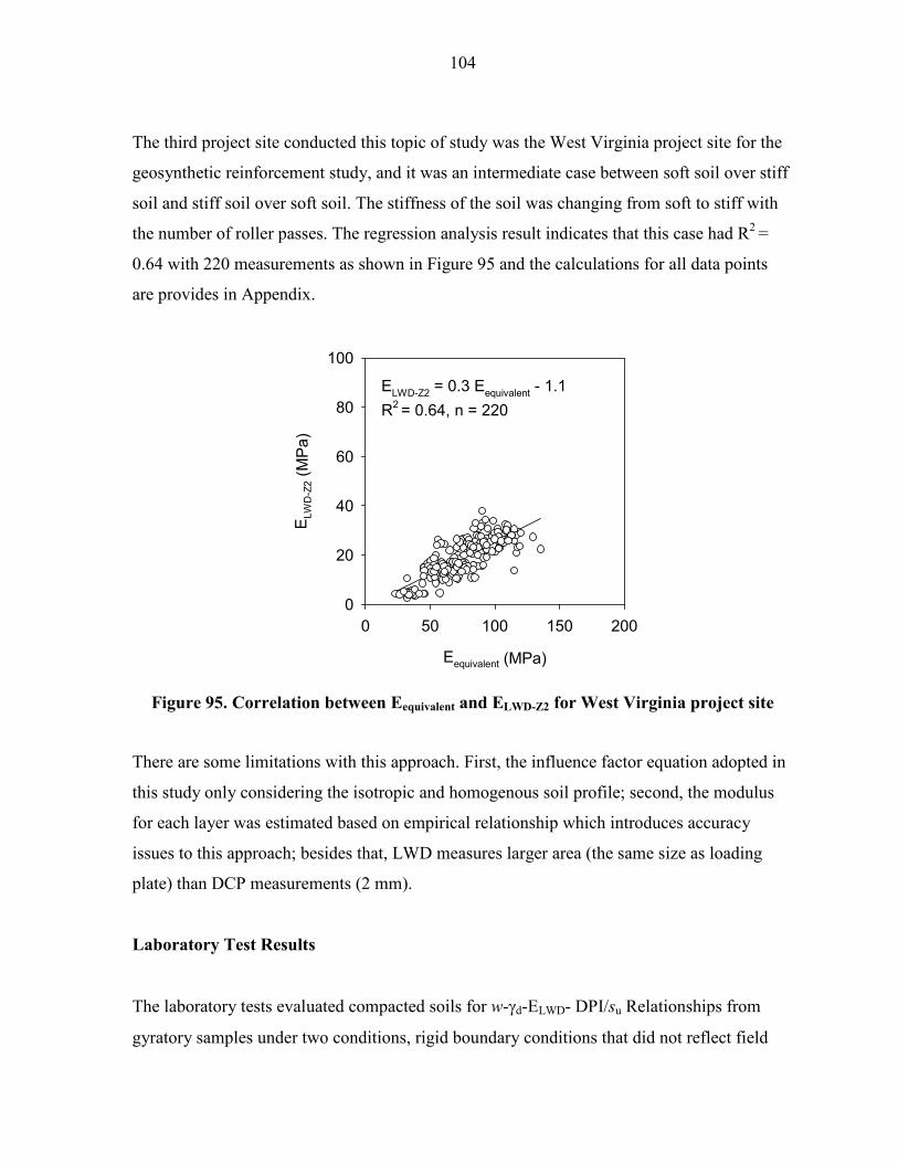
104

The third project site conducted this topic of study was the West Virginia project site for the

geosynthetic reinforcement study, and it was an intermediate case between soft soil over stiff

soil and stiff soil over soft soil. The stiffness of the soil was changing from soft to stiff with

the number of roller passes. The regression analysis result indicates that this case had R2 =

0.64 with 220 measurements as shown in Figure 95 and the calculations for all data points

are provides in Appendix.

Figure 95. Correlation between Eequivalent and ELWD-Z2 for West Virginia project site

There are some limitations with this approach. First, the influence factor equation adopted in

this study only considering the isotropic and homogenous soil profile; second, the modulus

for each layer was estimated based on empirical relationship which introduces accuracy

issues to this approach; besides that, LWD measures larger area (the same size as loading

plate) than DCP measurements (2 mm).

Laboratory Test Results

The laboratory tests evaluated compacted soils for w-γd-ELWD- DPI/su Relationships from

gyratory samples under two conditions, rigid boundary conditions that did not reflect field

Eequivalent (MPa)

0 50 100 150 200

ELW

D-Z2 (M

Pa)

0

20

40

60

80

100

ELWD-Z2 = 0.3 Eequivalent - 1.1

R2 = 0.64, n = 220

105

conditions and flexible boundary conditions that more closely matched field conditions.

Results from rigid boundary conditions

Three types of materials were tested in this topic of research, which were US 10 granular

materials, TH 36 silty clay, and TH 60 non-granular material. DPI, su, and ELWD

measurements obtained on gyratory compacted specimens confined with the rigid boundary

condition. Multiple regression analysis was performed to determine the relationships between

ELWD, w and γd. Statistical significance of each variable was assessed based on p- and t-

values. The selected criteria for identifying the significance of a parameter include: p- value

< 0.05 = significant, < 0.10 = possibly significant, > 0.10 = not significant, and t- value < -2

or > +2 = significant. The p- value indicates the significance of a parameter and the t- ratio

value indicates the relative importance. The multiple regression relationships obtained are

presented as contour plots in relationship with Proctor w and γd relationships for all the three

types of materials as shown from Figure 96 to Figure 101. The regression relationships are

summarized in Table 17 including R2 vlues which range from 0.7 to 0.9. An advantage of

presenting the results in contour format is that the ELWD or DPI “target” values with respect

to acceptable w and γd can be graphically determined and the influence of moisture content is

clearly evident. The statistical model output figures are provided in Appendix.

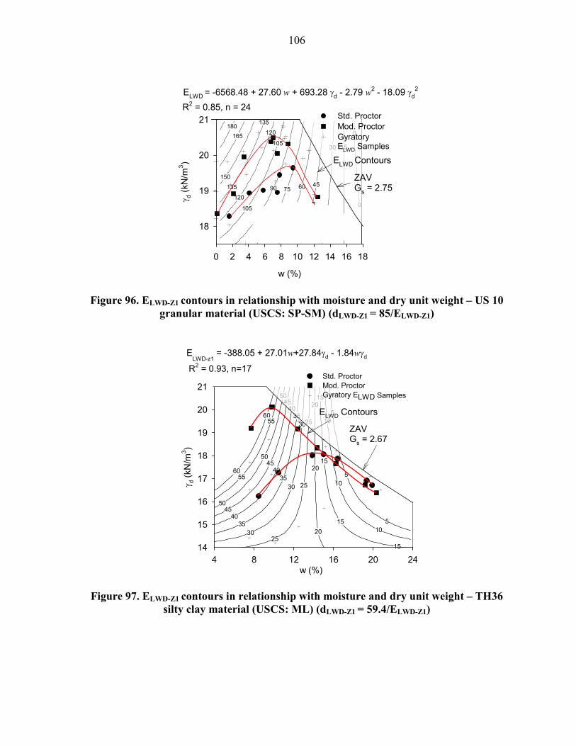
106

Figure 96. ELWD-Z1 contours in relationship with moisture and dry unit weight – US 10 granular material (USCS: SP-SM) (dLWD-Z1 = 85/ELWD-Z1)

Figure 97. ELWD-Z1 contours in relationship with moisture and dry unit weight – TH36 silty clay material (USCS: ML) (dLWD-Z1 = 59.4/ELWD-Z1)

0

0

15

15

30

30

45607590

105

105

120

120

135

135

150

165

180

w (%)

0 2 4 6 8 10 12 14 16 18

γ d (kN

/m3 )

18

19

20

21 Std. ProctorMod. ProctorGyratoryELWD Samples

ZAVGs = 2.75

ELWD Contours

ELWD = -6568.48 + 27.60 w + 693.28 γd - 2.79 w2 - 18.09 γd

2

R2 = 0.85, n = 24

5

5

5

10

10

10

15

15

15

15

20

20

20

30

30

30

25

25

25

40

40

40

35

35

35

50

50

50

45

45

45

60

60

55

55

w (%)4 8 12 16 20 24

γ d (kN

/m3 )

14

15

16

17

18

19

20

21Std. ProctorMod. ProctorGyratory ELWD Samples

ELWD-z1

= -388.05 + 27.01w+27.84γd - 1.84wγd

R2 = 0.93, n=17

ELWD Contours

ZAVGs = 2.67

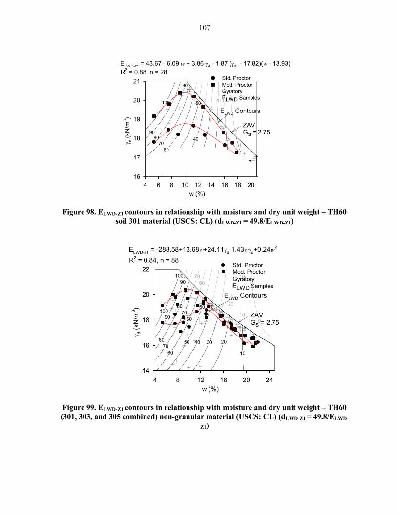
107

Figure 98. ELWD-Z1 contours in relationship with moisture and dry unit weight – TH60 soil 301 material (USCS: CL) (dLWD-Z1 = 49.8/ELWD-Z1)

Figure 99. ELWD-Z1 contours in relationship with moisture and dry unit weight – TH60 (301, 303, and 305 combined) non-granular material (USCS: CL) (dLWD-Z1 = 49.8/ELWD-

Z1)

0

0

10

10

20

20

30

30

40

50

50

60

60

70

70

80

80

90

100

w (%)4 6 8 10 12 14 16 18 20

γ d (kN

/m3 )

16

17

18

19

20

21 Std. ProctorMod. ProctorGyratoryELWD Samples

ZAVGs = 2.75

ELWD Contours

ELWD-z1 = 43.67 - 6.09 w + 3.86 γd - 1.87 (γd - 17.82)(w - 13.93)R2 = 0.88, n = 28

0

0

10

10

10

20

20

30

30

40

40

50

50

60

60

60

70

70

70

80

80

90

90

100

100

w (%)4 8 12 16 20 24

γ d (kN

/m3 )

14

16

18

20

22Std. ProctorMod. ProctorGyratoryELWD Samples

ZAVGs = 2.75

ELWD Contours

ELWD-z1 = -288.58+13.68w+24.11γd-1.43wγd+0.24w2

R2 = 0.84, n = 88

108

Figure 100. DPI contours in relationship with moisture and dry unit weight – TH60 non-granular material (301, 303, and 305 combined) (USCS: CL)

Figure 101. su contours in relationship with moisture and dry unit weight – TH60 non-granular material (301, 303, and 305 combined) (USCS: CL) (su determined from

empirical relationship with DPI)

160

160

160120

120

12080

80

80

60

6040

40

20

20

20

w (%)4 8 12 16 20 24

γ d (kN

/m3 )

14

16

18

20

22 Std. ProctorDCP Samples

Mod. Proctor

ZAVGs = 2.72

DPI = 284.09-32.28w-13.32γd+1.17wγd+0.77w2

R2=0.79, n=70

DPI Contours

12

1212

8

8

4

4

80

80

80

160

160

160240

240

240320

320

320

400

400

480

480560

560640

640720

720

800

w (%)4 8 12 16 20 24

γ d (kN

/m3 )

14

16

18

20

22 Std. ProctorDCP Samples

Mod. Proctor

ZAVGs = 2.72

su = -9565.44+289.5w+972.9γd-19.44wγd-21.31γd2

R2=0.71, n=70

su Contours

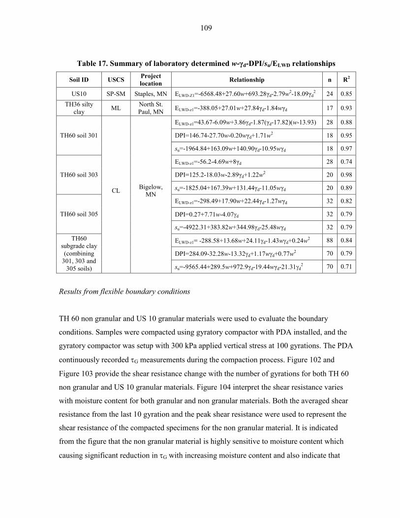
109

Table 17. Summary of laboratory determined w-γd-DPI/su/ELWD relationships

Soil ID USCS Project location Relationship n R2

US10 SP-SM Staples, MN ELWD-Z1=-6568.48+27.60w+693.28γd-2.79w2-18.09γd2 24 0.85

TH36 silty clay ML North St.

Paul, MN ELWD-z1=-388.05+27.01w+27.84γd-1.84wγd 17 0.93

TH60 soil 301

CL

Bigelow, MN

ELWD-z1=43.67-6.09w+3.86γd-1.87(γd-17.82)(w-13.93) 28 0.88

DPI=146.74-27.70w-0.20wγd+1.71w2 18 0.95

su=-1964.84+163.09w+140.90γd-10.95wγd 18 0.97

TH60 soil 303

ELWD-z1=-56.2-4.69w+8γd 28 0.74

DPI=125.2-18.03w-2.89γd+1.22w2 20 0.98

su=-1825.04+167.39w+131.44γd-11.05wγd 20 0.89

TH60 soil 305

ELWD-z1=-298.49+17.90w+22.44γd-1.27wγd 32 0.82

DPI=0.27+7.71w-4.07γd 32 0.79

su=-4922.31+383.82w+344.98γd-25.48wγd 32 0.79

TH60 subgrade clay (combining

301, 303 and 305 soils)

ELWD-z1= -288.58+13.68w+24.11γd-1.43wγd+0.24w2 88 0.84

DPI=284.09-32.28w-13.32γd+1.17wγd+0.77w2 70 0.79

su=-9565.44+289.5w+972.9γd-19.44wγd-21.31γd2 70 0.71

Results from flexible boundary conditions

TH 60 non granular and US 10 granular materials were used to evaluate the boundary

conditions. Samples were compacted using gyratory compactor with PDA installed, and the

gyratory compactor was setup with 300 kPa applied vertical stress at 100 gyrations. The PDA

continuously recorded τG measurements during the compaction process. Figure 102 and

Figure 103 provide the shear resistance change with the number of gyrations for both TH 60

non granular and US 10 granular materials. Figure 104 interpret the shear resistance varies

with moisture content for both granular and non granular materials. Both the averaged shear

resistance from the last 10 gyration and the peak shear resistance were used to represent the

shear resistance of the compacted specimens for the non granular material. It is indicated

from the figure that the non granular material is highly sensitive to moisture content which

causing significant reduction in τG with increasing moisture content and also indicate that

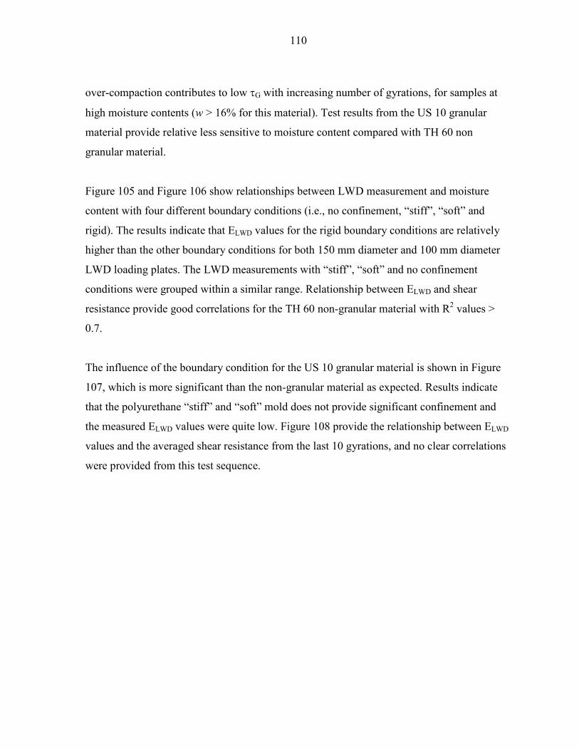
110

over-compaction contributes to low τG with increasing number of gyrations, for samples at

high moisture contents (w > 16% for this material). Test results from the US 10 granular

material provide relative less sensitive to moisture content compared with TH 60 non

granular material.

Figure 105 and Figure 106 show relationships between LWD measurement and moisture

content with four different boundary conditions (i.e., no confinement, “stiff”, “soft” and

rigid). The results indicate that ELWD values for the rigid boundary conditions are relatively

higher than the other boundary conditions for both 150 mm diameter and 100 mm diameter

LWD loading plates. The LWD measurements with “stiff”, “soft” and no confinement

conditions were grouped within a similar range. Relationship between ELWD and shear

resistance provide good correlations for the TH 60 non-granular material with R2 values >

0.7.

The influence of the boundary condition for the US 10 granular material is shown in Figure

107, which is more significant than the non-granular material as expected. Results indicate

that the polyurethane “stiff” and “soft” mold does not provide significant confinement and

the measured ELWD values were quite low. Figure 108 provide the relationship between ELWD

values and the averaged shear resistance from the last 10 gyrations, and no clear correlations

were provided from this test sequence.

111

Figure 102. Shear resistance versus number of gyrations (σσσσo = 300 kPa) for TH 60 soil 306 (USCS: CL)

Figure 103. Shear resistance versus number of gyrations for US10 granular material (USCS: SP-SM) (σo = 300 kPa)

LWD test - No confinement

0 20 40 60 80 100

τ G(kPa)

20

30

40

50

60

70

80

90LWD test - Soft boundary

0 20 40 60 80 10020

30

40

50

60

70

80

90

LWD test - Stiff boundary

Number of Gyrations

0 20 40 60 80 100

τ G(kPa)

20

30

40

50

60

70

80

90LWD test - Rigid boundary

Number of Gyrations

0 20 40 60 80 10020

30

40

50

60

70

80

90

w = 12.4%w = 13.6% w = 16.0%

w = 16.0%

w = 18.5%

w = 18.2%

w=15.9%

w = 15.3%

w = 15.4%w = 12.4%

w = 18.4%

w = 18.5%

w = 12.4%

w = 15.5% w = 15.5%

w = 16.6%

w = 18.0%

w = 18.5%

w=12.2%

w = 14.3%

w = 15.4%

w = 17.6%w = 16.6%

w = 17.6%

LWD test sample - Stiff boundary

Number of Gyrations

0 20 40 60 80 100

τ G(kPa)

40

50

60

70

80

90

100

w = 6.1%w = 8.0%w = 8.0%w = 10.0%w = 10.5%

LWD test sample - Rigid boundary

Number of Gyrations

0 20 40 60 80 10040

50

60

70

80

90

100

w = 6.0%w = 7.1%w = 8.0%w = 9.9%w = 10.3%

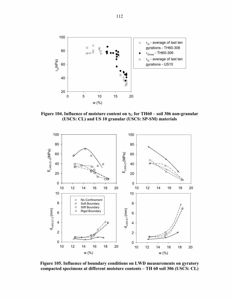
112

Figure 104. Influence of moisture content on ττττG for TH60 – soil 306 non-granular (USCS: CL) and US 10 granular (USCS: SP-SM) materials

Figure 105. Influence of boundary conditions on LWD measurements on gyratory compacted specimens at different moisture contents – TH 60 soil 306 (USCS: CL)

w (%)

0 5 10 15 20

τ G(kPa)

20

40

60

80

100τG - average of last tengyrations - TH60-306τGmax - TH60-306

τG - average of last ten gyrations - US10

10 12 14 16 18 20

ELW

D-Z1.5(MPa)

0

20

40

60

80

100

w (%)

10 12 14 16 18 20

d LWD-Z1.5 (m

m)

0

2

4

6

8

10

10 12 14 16 18 20

ELW

D-Z1(MPa)

0

20

40

60

80

100

w (%)

10 12 14 16 18 20

d LWD-Z1 (m

m)

0

2

4

6

8

10

No ConfinementSoft BoundaryStiff BoundaryRigid Boundary

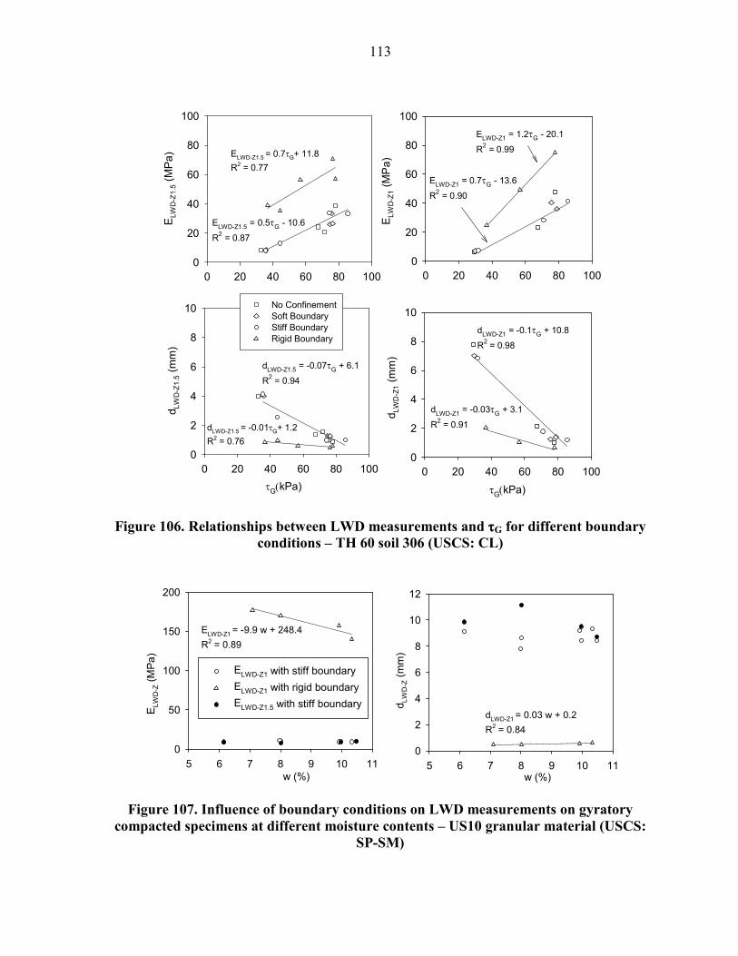
113

Figure 106. Relationships between LWD measurements and ττττG for different boundary conditions – TH 60 soil 306 (USCS: CL)

Figure 107. Influence of boundary conditions on LWD measurements on gyratory compacted specimens at different moisture contents – US10 granular material (USCS:

SP-SM)

τG(kPa)

0 20 40 60 80 100

d LWD-Z1.5 (m

m)

0

2

4

6

8

10

0 20 40 60 80 100

ELW

D-Z1.5 (M

Pa)

0

20

40

60

80

100

No ConfinementSoft BoundaryStiff BoundaryRigid Boundary

0 20 40 60 80 100

ELW

D-Z1 (M

Pa)

0

20

40

60

80

100

τG(kPa)

0 20 40 60 80 100

d LWD-Z1 (m

m)

0

2

4

6

8

10

ELWD-Z1.5 = 0.7τG+ 11.8

R2 = 0.77

ELWD-Z1.5 = 0.5τG - 10.6

R2 = 0.87

ELWD-Z1 = 1.2τG - 20.1

R2 = 0.99

ELWD-Z1 = 0.7τG - 13.6

R2 = 0.90

dLWD-Z1.5 = -0.07τG + 6.1

R2 = 0.94

dLWD-Z1.5 = -0.01τG+ 1.2

R2 = 0.76

dLWD-Z1 = -0.1τG + 10.8

R2 = 0.98

dLWD-Z1 = -0.03τG + 3.1

R2 = 0.91

w (%)5 6 7 8 9 10 11

ELW

D-Z (MPa)

0

50

100

150

200

ELWD-Z1 with stiff boundaryELWD-Z1 with rigid boundaryELWD-Z1.5 with stiff boundary

w (%)5 6 7 8 9 10 11

d LWD-Z (mm)

0

2

4

6

8

10

12

ELWD-Z1 = -9.9 w + 248.4

R2 = 0.89

dLWD-Z1 = 0.03 w + 0.2

R2 = 0.84

114

Figure 108. Relationship between LWD measurements and ττττG for different boundary conditions – US10 granular material (USCS: SP-SM)

Relationship between PDA Shear Resistance and Undrained Shear Strength

Unconfined compression (UC) tests were performed on gyratory compacted specimens to

investigate the relationship between τG and su. Due to the large amount of soil involved,

western Iowa loess (USCS: ML) was used for this topic of study. Samples were prepared at

six different moisture contents, which were -9%, -6%, -3%, 0%, +3% and +6% of optimum

moisture content from standard Proctor test. Samples were compacted with applied stress of

100 kPa, 300 kPa and 600 kPa at 100 gyrations. τG versus number of gyrations is presented

in Figure 109 for all specimens. Results show increasing shear resistance with increasing

number of gyrations up to about 15 gyrations and then no significant increase up to 100

gyrations for samples with w < 17%. Shear softening was observed at high moisture contents

(w > 18%) with number of gyration increase. Figure 110 shown the τG and su change with

moisture content for all the tested specimens, and it is clear shown from the figure that the τG

and su increase with the applied stress increase. Figure 111 provide strong correlation

between τG and su measured from the same specimen with R2 = 0.94. On average, the su is

about 1.6 times τG.

τG (kPa)

70 75 80 85 90 95

ELW

D-Z (MPa)

0

50

100

150

200

τG (kPa)

70 75 80 85 90 95

d LWD-Z (mm)

0

2

4

6

8

10

12

ELWD-Z1 with stiff boundary

ELWD-Z1 with rigid boundary

ELWD-Z1.5 with stiff boundary

115

Figure 109. ττττG versus number of gyrations for loess (USCS: ML)

w = 8.5%

0 20 40 60 80 100

τ G (kP

a)

0

50

100

150

200

w = 11.3%

0 20 40 60 80 1000

50

100

150

200

w =14.0%

0 20 40 60 80 100

τ G (kP

a)

0

50

100

150

200

w =16.9%

0 20 40 60 80 1000

50

100

150

200

w = 21.8%

Number of Gyrations

0 20 40 60 80 100

τ G (kP

a)

0

50

100

150

200

w = 21.8%

Number of Gyrations

0 20 40 60 80 1000

50

100

150

200

σo = 100 kPa

σo = 300 kPa

σo = 600 kPa

w = 7.8%

w = 7.6%

w = 10.5%

w = 10.3%

w = 13.2%

w = 13.6%

w = 16.1%

w = 16.3%

w = 19.7%

w = 18.4% w = 22.3%w = 22.1%

116

Figure 110. su and ττττG versus moisture content for gyratory compacted specimens after 100 gyrations at σσσσo = 100, 300, and 600 kPa for loess (USCS: ML)

Figure 111. Relationship between su and ττττG for loess (USCS: ML)

Relationship between PDA Shear Resistance and Resilient Modulus

Resilient modulus (Mr) tests and unconsolidated-undrained triaxial compression (UU) tests

were performed on gyratory compacted specimens with the height to diameter ratio of H/D =

1:1 and H/D = 2:1. The H/D = 1:1 specimens were directly produced from the gyratory

w (%)

6 9 12 15 18 21 24

s u (kP

a)

0

100

200

300

400

τ G (kP

a)

0

50

100

150

200

250100 kPa su300 kPa su600 kPa su100 kPa τG

300 kPa τG

600 kPa τG

τG (kPa)

0 100 200 300 400

su (kPa)

0

100

200

300

400

su = 1.6 τG + 24.8

R2 = 0.94

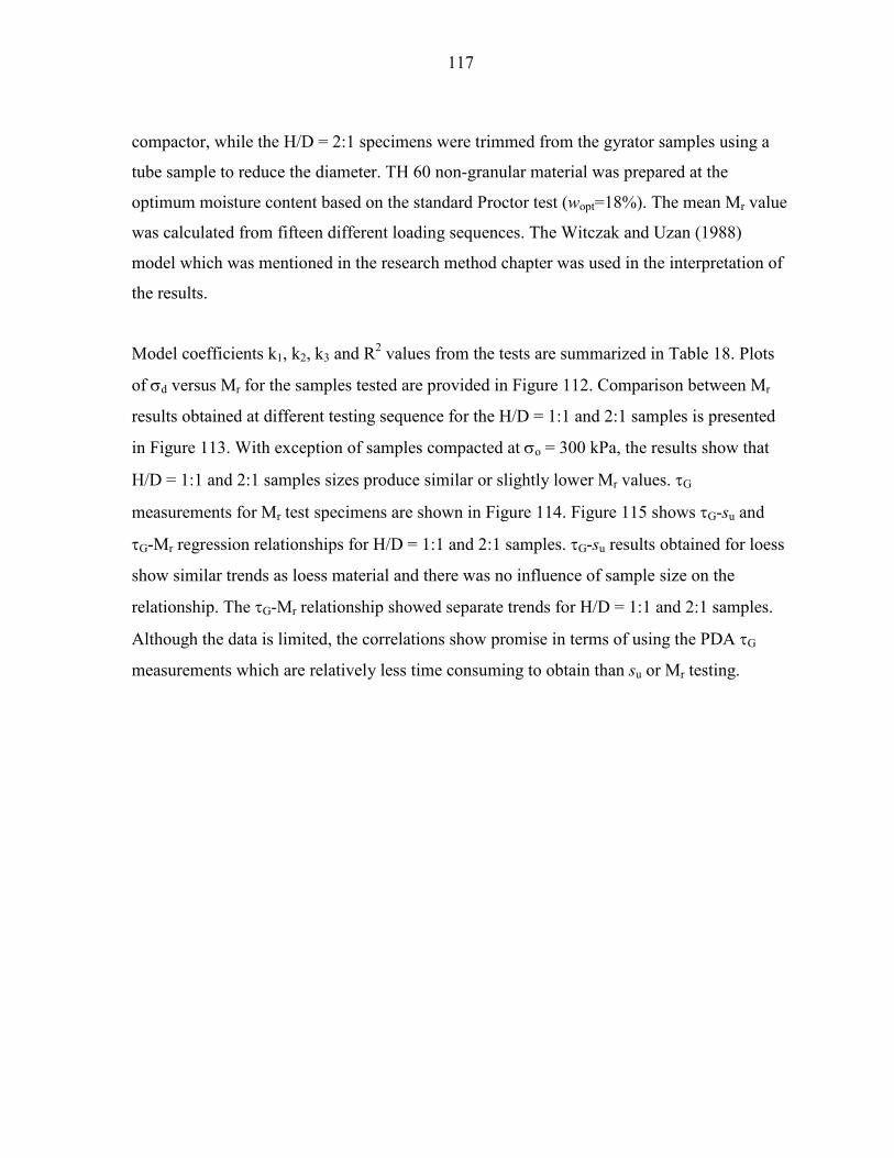
117

compactor, while the H/D = 2:1 specimens were trimmed from the gyrator samples using a

tube sample to reduce the diameter. TH 60 non-granular material was prepared at the

optimum moisture content based on the standard Proctor test (wopt=18%). The mean Mr value

was calculated from fifteen different loading sequences. The Witczak and Uzan (1988)

model which was mentioned in the research method chapter was used in the interpretation of

the results.

Model coefficients k1, k2, k3 and R2 values from the tests are summarized in Table 18. Plots

of σd versus Mr for the samples tested are provided in Figure 112. Comparison between Mr

results obtained at different testing sequence for the H/D = 1:1 and 2:1 samples is presented

in Figure 113. With exception of samples compacted at σo = 300 kPa, the results show that

H/D = 1:1 and 2:1 samples sizes produce similar or slightly lower Mr values. τG

measurements for Mr test specimens are shown in Figure 114. Figure 115 shows τG-su and

τG-Mr regression relationships for H/D = 1:1 and 2:1 samples. τG-su results obtained for loess

show similar trends as loess material and there was no influence of sample size on the

relationship. The τG-Mr relationship showed separate trends for H/D = 1:1 and 2:1 samples.

Although the data is limited, the correlations show promise in terms of using the PDA τG

measurements which are relatively less time consuming to obtain than su or Mr testing.

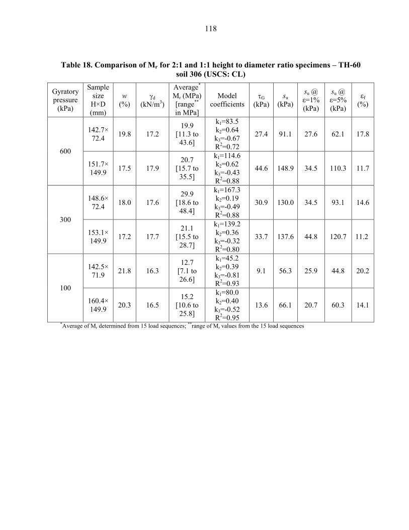
118

Table 18. Comparison of Mr for 2:1 and 1:1 height to diameter ratio specimens – TH-60 soil 306 (USCS: CL)

Gyratory pressure

(kPa)

Sample size H×D (mm)

w (%)

γd (kN/m3)

Average* Mr (MPa) [range** in MPa]

Model coefficients

τG (kPa)

su (kPa)

su @ ε=1% (kPa)

su @ ε=5% (kPa)

εf (%)

600

142.7×72.4 19.8 17.2

19.9 [11.3 to

43.6]

k1=83.5 k2=0.64 k3=-0.67 R2=0.72

27.4 91.1 27.6 62.1 17.8

151.7×149.9 17.5 17.9

20.7 [15.7 to

35.5]

k1=114.6 k2=0.62 k3=-0.43 R2=0.88

44.6 148.9 34.5 110.3 11.7

300

148.6×72.4 18.0 17.6

29.9 [18.6 to

48.4]

k1=167.3 k2=0.19 k3=-0.49 R2=0.88

30.9 130.0 34.5 93.1 14.6

153.1×149.9 17.2 17.7

21.1 [15.5 to

28.7]

k1=139.2 k2=0.36 k3=-0.32 R2=0.80

33.7 137.6 44.8 120.7 11.2

100

142.5×71.9 21.8 16.3

12.7 [7.1 to 26.6]

k1=45.2 k2=0.39 k3=-0.81 R2=0.93

9.1 56.3 25.9 44.8 20.2

160.4×149.9 20.3 16.5

15.2 [10.6 to

25.8]

k1=80.0 k2=0.40 k3=-0.52 R2=0.95

13.6 66.1 20.7 60.3 14.1

*Average of Mr determined from 15 load sequences; **range of Mr values from the 15 load sequences

119

Figure 112. Effect of height to diameter ratio (H/D = 1 and 2) on Mr of gyratory compacted specimens at σσσσo = 100, 300 and 600 kPa at 100 gyrations –TH-60 soil 306

(USCS: CL)

Deviator Stress, σd (kPa)

0 10 20 30 40 50 60 70 80

Resilient M

odulus, M

r (MPa)

0

10

20

30

40

50

Deviator Stress, σd (kPa)

0 10 20 30 40 50 60 70 80

Resilient M

odulus, M

r (MPa)

0

10

20

30

40

50

H/D = 1:1H/D = 2:1

Deviator Stress, σd (kPa)

0 10 20 30 40 50 60 70 80

Resilient M

odulus, M

r (MPa)

0

10

20

30

40

50σo = 600 kPa (100 gyrations)

σo=300 kPa (100 gyrations)

σo=100 kPa (gyrations)

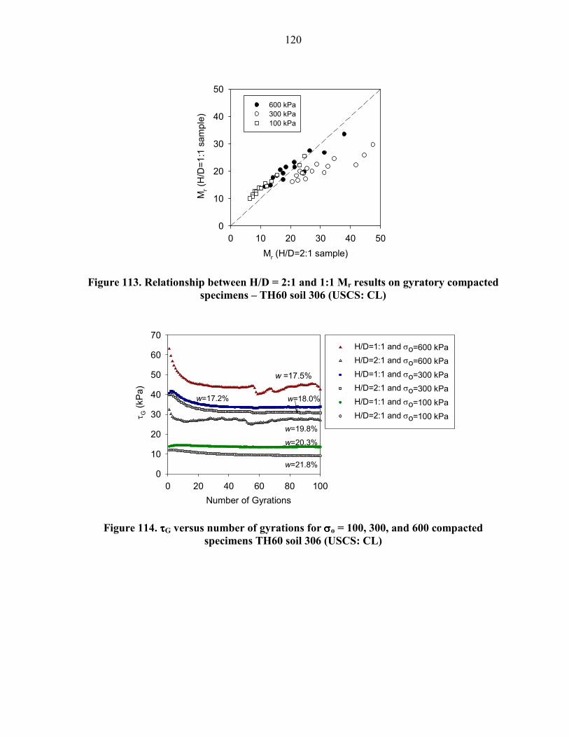
120

Figure 113. Relationship between H/D = 2:1 and 1:1 Mr results on gyratory compacted specimens – TH60 soil 306 (USCS: CL)

Figure 114. ττττG versus number of gyrations for σσσσo = 100, 300, and 600 compacted specimens TH60 soil 306 (USCS: CL)

Mr (H/D=2:1 sample)

0 10 20 30 40 50

Mr (H/D=1

:1 sam

ple)

0

10

20

30

40

50

600 kPa300 kPa100 kPa

w =17.5%

Number of Gyrations

0 20 40 60 80 100

τ G (kP

a)

0

10

20

30

40

50

60

70H/D=1:1 and σo=600 kPa

H/D=2:1 and σo=600 kPa

H/D=1:1 and σo=300 kPa

H/D=2:1 and σo=300 kPa

H/D=1:1 and σo=100 kPa

H/D=2:1 and σo=100 kPa

w=17.2% w=18.0%

w=19.8%

w=20.3%

w=21.8%

121

Figure 115. Correlation between su, Mr and ττττG for samples with H/D = 1 and 2 – TH 60 soil 306 (USCS: CL)

Establish Field Target Values for Quality Assurance

Field ELWD target value determination study consists of performing LWD test with 200 mm

diameter loading plate on uncompacted material. The idea was that with multiple hammer

drops the soil would compact and the ELWD value would reach an asymptote thus establishing

a field target value. Results are presented in Figure 116 for field tests at TH 60 in non-

granular soil. Results indicated that with increasing number of drops ELWD increases and

dLWD decrease to approach an asymptotic value. Moisture contents for each tested point are

provided and were in the range of 9.5 to 12.4%. ELWD values ranged from about 6 MPa to 16

MPa. No trend was observed in the ELWD or dLWD values with moisture content.

τG (kPa)

0 80 160 240 320 400

s u (kPa)

0

80

160

240

320

400

TH60-306 H/D = 1:1 TH60-306 H/D = 2:1Loess H/D = 1:1

τG (kPa)

0 10 20 30 40 50

Mr (MPa)

0

10

20

30

40

50

H/D = 1:1 H/D = 2:1 su = 1.85 τG

R2 = 0.79

R2 = 0.80

R2 = 0.85

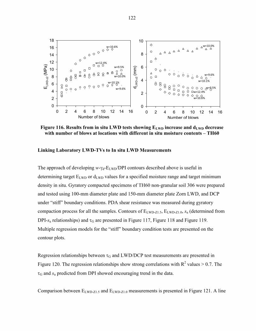
122

Figure 116. Results from in situ LWD tests showing ELWD increase and dLWD decrease with number of blows at locations with different in situ moisture contents – TH60

Linking Laboratory LWD-TVs to In situ LWD Measurements

The approach of developing w-γd-ELWD/DPI contours described above is useful in

determining target ELWD or dLWD values for a specified moisture range and target minimum

density in situ. Gyratory compacted specimens of TH60 non-granular soil 306 were prepared

and tested using 100-mm diameter plate and 150-mm diameter plate Zorn LWD, and DCP

under “stiff” boundary conditions. PDA shear resistance was measured during gyratory

compaction process for all the samples. Contours of ELWD-Z1.5, ELWD-Z1.0, su (determined from

DPI-su relationships) and τG are presented in Figure 117, Figure 118 and Figure 119.

Multiple regression models for the “stiff” boundary condition tests are presented on the

contour plots.

Regression relationships between τG and LWD/DCP test measurements are presented in

Figure 120. The regression relationships show strong correlations with R2 values > 0.7. The

τG and su predicted from DPI showed encouraging trend in the data.

Comparison between ELWD-Z1.5 and ELWD-Z1.0 measurements is presented in Figure 121. A line

Number of blows0 2 4 6 8 10 12 14 16

ELW

D-z2 (M

Pa)

0

2

4

6

8

10

12

14

16

18

Number of blows0 2 4 6 8 10 12 14 16

d LWD-z2 (m

m)

0

2

4

6

8

10

w=9.6%

w=10.1%

w=10.6%

w=12.4%w=9.5%

w=10.0% w=9.6%

w=10.1%

w=10.6%

w=12.4%w=9.5%

w=10.0%

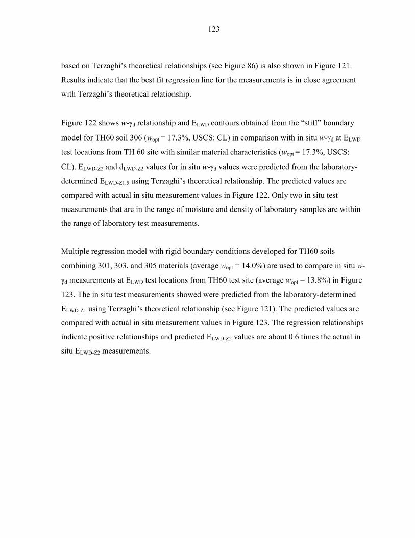
123

based on Terzaghi’s theoretical relationships (see Figure 86) is also shown in Figure 121.

Results indicate that the best fit regression line for the measurements is in close agreement

with Terzaghi’s theoretical relationship.

Figure 122 shows w-γd relationship and ELWD contours obtained from the “stiff” boundary

model for TH60 soil 306 (wopt = 17.3%, USCS: CL) in comparison with in situ w-γd at ELWD

test locations from TH 60 site with similar material characteristics (wopt = 17.3%, USCS:

CL). ELWD-Z2 and dLWD-Z2 values for in situ w-γd values were predicted from the laboratory-

determined ELWD-Z1.5 using Terzaghi’s theoretical relationship. The predicted values are

compared with actual in situ measurement values in Figure 122. Only two in situ test

measurements that are in the range of moisture and density of laboratory samples are within

the range of laboratory test measurements.

Multiple regression model with rigid boundary conditions developed for TH60 soils

combining 301, 303, and 305 materials (average wopt = 14.0%) are used to compare in situ w-

γd measurements at ELWD test locations from TH60 test site (average wopt = 13.8%) in Figure

123. The in situ test measurements showed were predicted from the laboratory-determined

ELWD-Z1 using Terzaghi’s theoretical relationship (see Figure 121). The predicted values are

compared with actual in situ measurement values in Figure 123. The regression relationships

indicate positive relationships and predicted ELWD-Z2 values are about 0.6 times the actual in

situ ELWD-Z2 measurements.

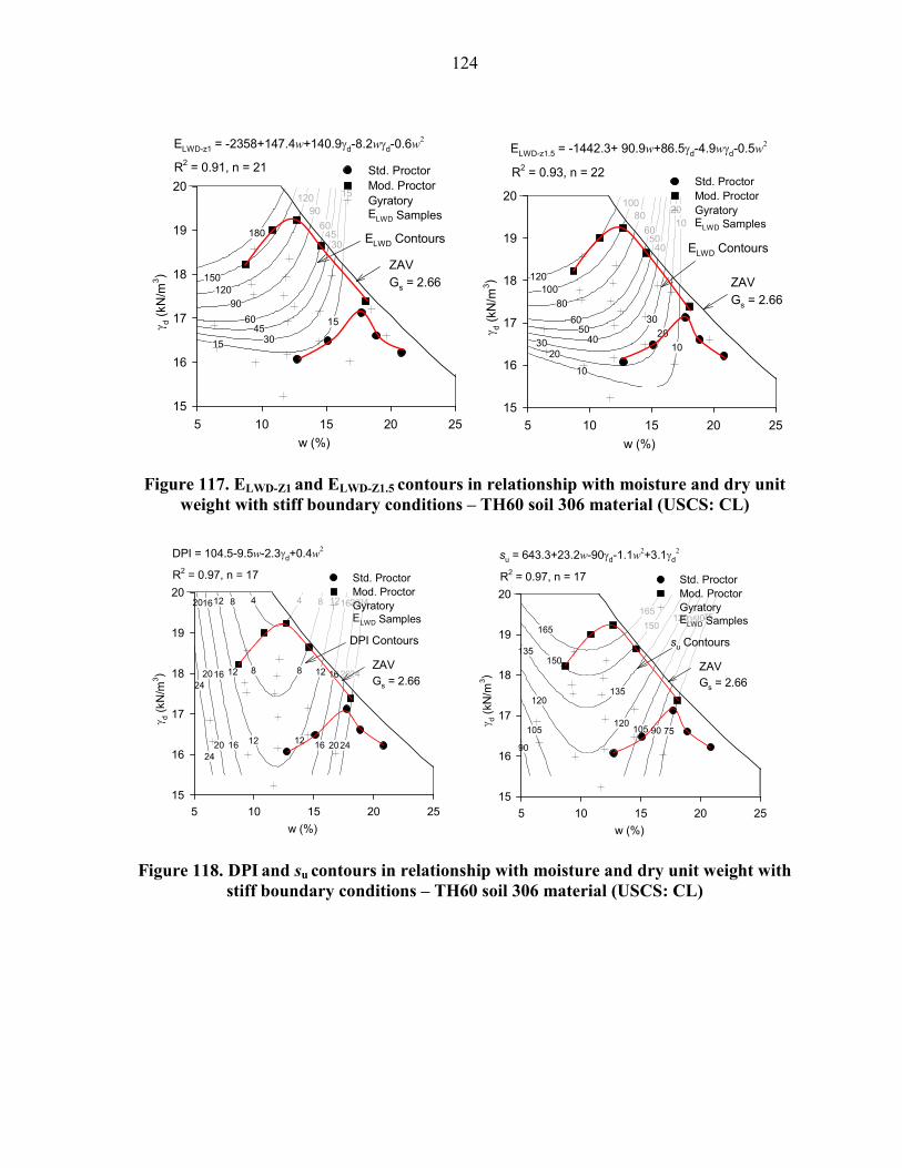
124

Figure 117. ELWD-Z1 and ELWD-Z1.5 contours in relationship with moisture and dry unit weight with stiff boundary conditions – TH60 soil 306 material (USCS: CL)

Figure 118. DPI and su contours in relationship with moisture and dry unit weight with stiff boundary conditions – TH60 soil 306 material (USCS: CL)

15

15

15

45

45

30

30

60

60

90

90

120

120

150

180

w (%)5 10 15 20 25

γ d (kN

/m3 )

15

16

17

18

19

20Std. ProctorMod. ProctorGyratoryELWD Samples

ZAVGs = 2.66

ELWD Contours

ELWD-z1 = -2358+147.4w+140.9γd-8.2wγd-0.6w2

R2 = 0.91, n = 21

10

10

20

20

20

30

3050

50

40

40

10

60

60

80

80

100

100

120

w (%)5 10 15 20 25

γ d (kN

/m3 )

15

16

17

18

19

20Std. ProctorMod. ProctorGyratoryELWD Samples

ZAVGs = 2.66

ELWD Contours

ELWD-z1.5 = -1442.3+ 90.9w+86.5γd-4.9wγd-0.5w2

R2 = 0.93, n = 22

24

24

24

20

20

2016

16

1612

12

1212

12

12 8

88

8 4416

16

16

20

20

20

24

24

w (%)5 10 15 20 25

γ d (kN

/m3 )

15

16

17

18

19

20Std. ProctorMod. ProctorGyratoryELWD Samples

ZAVGs = 2.66

DPI Contours

DPI = 104.5-9.5w-2.3γd+0.4w2

R2 = 0.97, n = 17

75

75

90

90

105

105120

120

120135

135150

150165

165

105

90

w (%)5 10 15 20 25

γ d (kN

/m3 )

15

16

17

18

19

20Std. ProctorMod. ProctorGyratoryELWD Samples

ZAVGs = 2.66

su Contours

su = 643.3+23.2w-90γd-1.1w2+3.1γd

2

R2 = 0.97, n = 17

125

Figure 119. ττττG contours in relationship with moisture and dry unit weight with stiff boundary test – TH60 soil 306 material (USCS: CL)

20

20

20

2040

40

40

80

80

120

120

160

160

200

200

240

w (%)5 10 15 20 25

γ d (kN

/m3 )

15

16

17

18

19

20Std. ProctorMod. ProctorGyratoryELWD Samples

ZAVGs = 2.66

τ Contours

τ = -2301.5+127.2w+148γd-8.1wγd

R2 = 0.97, n = 24

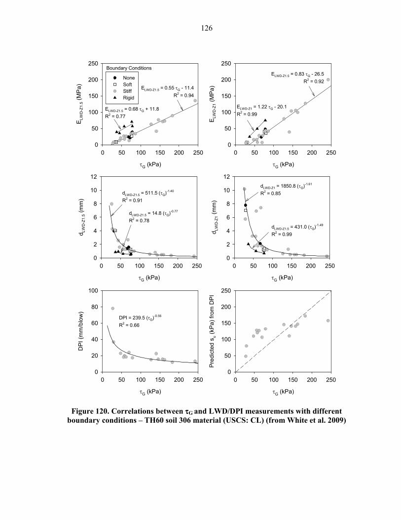
126

Figure 120. Correlations between ττττG and LWD/DPI measurements with different boundary conditions – TH60 soil 306 material (USCS: CL) (from White et al. 2009)

τG (kPa)

0 50 100 150 200 250

ELW

D-Z1.5 (M

Pa)

0

50

100

150

200

250

NoneSoftStiffRigid

τG (kPa)

0 50 100 150 200 250

ELW

D-Z1 (M

Pa)

0

50

100

150

200

250

τG (kPa)

0 50 100 150 200 250

d LWD-Z1.5 (m

m)

0

2

4

6

8

10

12

τG (kPa)

0 50 100 150 200 250

d LWD-Z1 (m

m)

0

2

4

6

8

10

12

Boundary Conditions

τG (kPa)

0 50 100 150 200 250

DPI (mm/blow)

0

20

40

60

80

100

τG (kPa)

0 50 100 150 200 250

Predicted

su (kPa) from

DPI

0

50

100

150

200

250

ELWD-Z1.5 = 0.55 τG - 11.4

R2 = 0.94

ELWD-Z1.5 = 0.68 τG + 11.8

R2 = 0.77

ELWD-Z1 = 1.22 τG - 20.1

R2 = 0.99

ELWD-Z1.5 = 0.83 τG - 26.5

R2 = 0.92

dLWD-Z1.5 = 511.5 (τG)-1.40

R2 = 0.91

dLWD-Z1.5 = 14.8 (τG)-0.77

R2 = 0.78

dLWD-Z1 = 1850.8 (τG)-1.61

R2 = 0.85

dLWD-Z1.5 = 431.0 (τG)-1.49

R2 = 0.99

DPI = 239.5 (τG)-0.56

R2 = 0.66

127

Figure 121. Relationships between laboratory ELWD-Z1 and ELWD-Z2 measurements in comparison with Terzaghi’s theoretical relationships – TH60 soil 306 material (USCS:

CL) (from White et al. 2009)

Figure 122. Comparison between in situ LWD measurements and laboratory predicted LWD target values (TH60 soil 306 “stiff” boundary model) (from White et al. 2009)

ELWD-Z1 (MPa)

0 50 100 150 200 250

ELW

D-Z1.5 (M

Pa)

0

50

100

150

200

250Measured ELWD-Z1.5

Least Squares Fit LinePredicted* ELWD-Z1.5

Predicted* ELWD-Z2

ELWD-Z1.5 = ELWD-Z1 x [1/1.5]

ELWD-Z1.5 = 0.74 ELWD-Z1

R2 = 0.92

ELWD-Z2 = ELWD-Z1 x [1/2]

*Using Terzaghi's theoretical relationshipfor clay soils (See Figure 5.10)

90

90

120

120

150

180

20

20

20

40

4060

60

w (%)5 10 15 20 25

γ d (kN

/m3 )

15

16

17

18

19

20

Std. ProctorMod. ProctorTest Strip 3in-situ w-γd

ZAVGs = 2.66

ELWD Contours

ELWD-z1 = -2358+147.4w+140.9γd-8.2wγd-0.6w2

R2 = 0.91, n = 21

10

1020

20

20

30

3050

50

40

40

10

60

60

80

80

100

100

120

w (%)5 10 15 20 25

γ d (kN

/m3 )

15

16

17

18

19

20 Std. ProctorMod. ProctorTest Strip 3in-situ w-γd

ZAVGs = 2.66

ELWD Contours

ELWD-z1.5 = -1442.3+ 90.9w+86.5γd-4.9wγd-0.5w2

R2 = 0.93, n = 22

Field Measured ELWD-Z2 (MPa)

0 10 20 30 40 50 60

Laboratory

Predicted E

LWD-Z2 (M

Pa)

0

10

20

30

40

50

60

Field Measured dLWD-Z2 (mm)

0 2 4 6 8 10 12 14

Laboratory

Predicted d

LWD-Z2 (m

m)

0

2

4

6

8

10

12

14

Stiff boundary,150 mm diameter LWD

Stiff boundary,150 mm diameter LWD

128

Figure 123. Comparison between in situ LWD measurements and laboratory predicted LWD target values (TH60 soil 301, 302, 303 combined rigid boundary model) (from

White et al. 2009)

0

0

10

10

10

20

20

30

30

40

40

50

50

60

60

60

70

70

70

80

80

90

90

100

100

w (%)4 8 12 16 20 24

γ d (kN

/m3 )

14

16

18

20

22 Std. ProctorMod. ProctorTest Strips 4/5 In-situ w-γdTest Strip 1In-situ w-γd

ZAVGs = 2.75

ELWD Contours

ELWD-z1 = -288.58+13.68w+24.11γd-1.43wγd+0.24w2

R2 = 0.84, n = 88

Field Measured dLWD-Z2 (mm)

0 2 4 6 8 10 12 14

Labo

ratory

Predicted d

LWD-Z2 (m

m)

0

2

4

6

8

10

12

14

Test Strip 4Test Strip 5Test Strip 1Test Strip 3

Field Measured ELWD-Z2 (MPa)

0 10 20 30 40 50 60

Labo

ratory

Predicted

ELW

D-Z2 (M

Pa)

0

10

20

30

40

50

60

Lab ELWD-Z2= 0.56 Field ELWD-Z2

R2=0.22

Rigid boundary,100 mm diameter LWD

Lab dLWD-Z2= 1.88 Field dLWD-Z2

R2=0.46

Rigid boundary,100 mm diameter LWD

129

CHAPTER 6. CONCLUSIONS AND RECOMMENDATIONS

The objectives of this study were to evaluate the use of mechanistic-based compaction

measurement devices such as light weight deflectometer (LWD), falling weight

deflectometer (FWD), plate load test (PLT), Briaud compaction device (BCD), and dynamic

cone penetrometer (DCP) for measuring the stiffness/strength of the compacted material; and

to gain a better understanding of the factors that affect these devices; and to evaluate

correlations between the measurements of these devices. A final objective for this study was

to develop an approach for target value determination for QC/QA using the LWD. Data were

collected from laboratory tests and from tests conducted at six field locations.

Some of the key findings obtained from this research are:

• Influence of plate diameter and plate contact stress on ELWD

o Limited data showed good correlations between different plate diameters, but

need more data to ensure statistically significant.

• Various factors affect correlations between LWD, FWD, PLT and BCD:

o Differences in applied contact stresses,

o Differences in deflection measurement method,

o Differences in measurement influence depths,

o Assumption of constant contact stress for LWD vs. measured stress for

FWD/BCD/PLT,

o Measurement errors associated with each device.

• The estimated Eequivalent provide relative good correlations with measured ELWD

using the approach adopted in this research (R2 = 0.5 to 0.7). However, the approach

has limitations.

• The relationships between the PDA τG values and other soil engineering parameters

(e.g., ELWD, Mr, su) showed good correlation coefficients (R2 > 0.7). A significant

advantage with using the PDA devices is that it is less time consuming than other test

methods (i.e., ELWD, UU, UC, or Mr tests).

130

The general recommendations for future study include:

• Obtain LWD measurements with different device configurations for a wide-variety of

soils.

• Different approaches for estimating Eequivalent need to considered and compared to

obtain the better correlation relationships.

• A new mold which can better simulate the actual field boundary condition needs to

develop for conducting the target value determination study in the laboratory,

• τG from PDA provide encouraging results in relating to the engineering properties of

the compacted material. Future studies should focus on linking τG to field

measurements.

131

REFERENCES

AASHTO. (1999). Standard method of test for determining the resilient modulus of soils and aggregate materials T-307, American Association of State Highway and Transportation Officials, Washington, D.C. ASTM. (1983). “Test method for compaction and shear properties of bituminous mixtures by means of the U.S. Corps of Engineers gyratory testing machine.” Annual book of ASTM Standards, ASTM D3387, West Conshohocken, PA. ASTM. (1993). “Standard test method for repetitive static plate load tests of soils and flexible pavement components, for use in evaluation and design of airport and highway pavements.” Annual book of ASTM Standards, ASTM D1195, West Conshohocken, PA. ASTM. (2000). “Test method for laboratory compaction characteristics of soils using standard effort.” Annual book of ASTM Standards, ASTM D698, West Conshohocken, PA. ASTM. (2000). “Test method for laboratory compaction characteristics of soils using modified effort.” Annual book of ASTM Standards, ASTM D1557, West Conshohocken, PA. ASTM. (2000). “Standard classification of soils for engineering purposes (Unified Soil Classification System).” Annual book of ASTM Standards, ASTM D2487, West Conshohocken, PA. ASTM. (2003). “Standard test method for unconsolidated-undrained triaxial compression test on cohesive soils.” Annual Book of ASTM Standards, ASTM D2850, West Conshohocken, PA. ASTM. (2003). “Standard test method for use of the dynamic cone penetrometer in shallow pavement applications.” Annual Book of ASTM Standards, ASTM D6951, West Conshohocken, PA. ASTM. (2005). “Test method for density of soil and soil aggregate inplace by nuclear methods (shallow depth).” Annual Book of ASTM Standards, ASTM D2922, West Conshohocken, PA. ASTM. (2005). “Test methods for liquid limit, plastic limit, and plasticity index of soils.” Annual Book of ASTM Standards, ASTM D4318, West Conshohocken, PA. ASTM. (2006). “Test method for unconfined compressive strength of cohesive soil.” Annual Book of ASTM Standards, ASTM D2166, West Conshohocken, PA. Bahia, H. U., and Paye, B.C. (2004). “Using gyratory compactor to measure mechanical stability of asphalt mixtures.” Final Report, WisDOT, Madison, WI.

132

Briaud, J., Li, Y., and Rhee, K. (2006). “BCD: a soil modulus device for compaction control.” Journal of Geotechnical and Geoenvironmental Engineering, Vol.132, No. 1, pp. 108-115. Burnham, T., (1996). Application of the Dynamic Cone Penetrometer to Mn/DOT’s Pavement Assessment Procedures, Revised Draft Report, Office of Minnesota Road Research. Chaddock, B. C. J., and Brown., A., (1995). “In situ Test for Road Foundation Assessment,” Proc., Unbound Aggregate in Roads – UNBAR 4. A. Dawson, and B. Jones, Eds., Nottingham, U.K. Chen, D., Lin, D., Liau, P. and Bilyeu, J. (2005). “A Correlation between Dynamic Cone Penetrometer Values and Pavement Layer Moduli.” Geotechnical Testing Journal, ASTM International, Vol. 28, No.1, p. 42-49 Coyle, H. M., and West, E. C. (1956). Laboratory compaction of a silty clay to simulate field density curves, MS Thesis, Massachusetts Institute of Technology, MA. Fleming, P. R., Lambert, J. P., Frost, M. W. and Rogers, C. D. “In situ assessment of stiffness modulus for highway foundations during construction.” In Proceedings of the 9th International Conference on Asphalt Pavements, Copenhagen, 2002. International Society for Asphalt Pavements, White Bear Lake, MN, USA, 2002, pp. 1–12 (CD-ROM). Fleming, P.R., Frost, M.W., and Lambert, J.P., (2007). “Review of Light Weight Deflectometer for Routine In Situ Assessment of Pavement Material Stiffness.” Transportation Research Record. 2004, Transportation Research Board, Washington D.C., 80-87. George, K.P., (2003). Falling Weight Deflectometer for Estimating Subgrade Resilient Moduli, Final Report FHWA/MS-DOT-RD-03. Mississippi Department of Transportation, Jackson, MS. Guler, M., Bahia, H. U., Bosscher, P. J., and Plesha, M. E. (1996). “Device for Measuring Shear Resistance of Hot-Mix Asphalt in Gyratory Compactor.” Transportation Research Record: Journal of the Transportation Research Board, No. 1723, 116-124. Gupta , S., Kang, D.H., Ranaivoson, A. (2009). Hydraulic, Mechanical, and Leaching Characteristics of Recylced Materials. Draft Report submitted Minnesota Department of Transportation, St. Paul, MN. Harrison, J.A. (1986). “Correlation of CBR and Dynamic Cone Penetrometer Strength Measurement of Soils” Australian Road Research, June 1986, Vol. 16, No.2, pp130-136. Kelyn, E.G. (1975), “The Use of the Dynamic Cone Penetrometer (DCP).” Report 2/74.

133

Transvaal Roads Department, Pretoria. Kim, W., and Labuz, J. (2006). Resilient modulus and strength of base course with recycled bituminous material, Final Report MN/RC 2007-05. Minnesota Department of Transportation, St. Paul, MN. KUAB (2009). Operation and technical reference manual: KUAB 2m-FWD model KUAB 150, Rättvik, Sweden. Li, Y. (2004). Use of a BCD for Compaction Control, Department of Civil Engineering, Texas A&M University, Ph.D. Lin. D., Liau, C., and Lin, J., (2006). “Factors Affecting Portable Falling Weight Deflectometer Measurements,” J. Geotech. Geoenviron. Eng., Vol. 132, No.6, 804-808. Livneh, M., Ishai, I., and Livneh, N., (1995). “Effect of the Vertical Confinement on Dynamic Cone Penetrometer Strength Values in Pavement and Subgrade Evaluations,” TRR 1473, pp. 1-8. Livneh, M., and I. Ishai. Pavement and Material Evaluation by a Dynamic Cone Penetrometer (1987), Proc., Sixth International Conference on the Structural Design of Asphalt Pavement, Vol. 1, Ann Arbor, Michigan, pp. 665-674. McElvaney, J., and Djatnika, I. (1991). “Strength evaluation of lime-stabilized pavement foundations using the dynamic cone penetrometer.” Australian Road Research, 21(1), 40-52. McRae, J. L. (1965). Gyratory testing machine technical manual for bituminous mixtures, soils, and base course materials, Engineering Developments Company, Inc., Vicksburg, MA. Mooney, M.A., and Miller, P.K., (2009). “Analysis of Lightweight Deflectometer Test Based on In Situ Stress and Strain Response.” J. Geotech. Geoenviron. Eng., Vol. 135, pp. 199-207. Odemark (1949). “Investigations as to the Elastic Properties of Soils and Design of Pavements according to the Theory of Elasticity,” Statens Väginstitut, Mitteilung No.77, Stockholm, Sweden. Pressure Distribution Analyzer, (2007). Operating manual, Test Quip LLC, Barnes, WI Powell, W. D., Potter, J. F., Mayhew, H. C., and Nunn, M. E., (1984). “The Structural Design of Bituminous Roads.” TRRL Report LR 1132, pp.62. Puppala, A.J., (2008). “Estimating Stiffness of Subgrade and Unbound Materials for Pavement Design,” NCHRP Project 20-5, Synthesis Topic 38-09, Transportation Research Board.

134

Rhee, K. (2008). PhD Dissertation, Texas A&M University, College Station, TX. Siekmeier, J. A., Young, D., and Beberg, D. (2000). “Comparison of the Dynamic Cone Penetrometer with Other Tests during Subgrade and Granular Base Characterization in Minnesota.” Nondestructive testing of pavements and backcalculation of moduli: ASTM STP 1375, S. D. Tayabji and E. O. Lukanen, eds., Vol. 3, ASTM, Philadelphia. Sridharan, A., Gandhi, and Suresh, S., (1990). “Stiffness Coefficients of Layered Soil Systems.” J. Geotech. Eng., Vol. 116, pp.604-624. Terzaghi, K., 1955, “Evaluation of Coefficient of Subgrade Reaction,” Geotechnique, Vol.5, No.4, pp.297-326. Ullidtz, Per. (1987). Pavement Analysis. Vol. 19. Amsterdam: Elsevier Science. Vennapusa, P.K., and White, D.J., (2009). “Comparison of Light Weight Deflectometer Measurements for Pavement Foundation Materials.” Geotechnical Testing Journal, Vol. 32, No.3, West Conshohocken, PA, p. 239-251. Webster, S.L., Grau, R.H., and Williams, R.P., (1992). “Description and Application of Dual Mass Dynamic Cone Penetrometer,” U.S. Army Engineer Waterways Experiment Station, Instruction Report, No. GL-92-3. Weidinger, D.M., Ge, L., (2009). “Laboratory Evaluation of the Briaud Compaction Device.” Journal of Geotechnical and Geoenvironmental Engineering. Vol. 135, No. 10, pp.1543-1546. White, D. J., Vennapusa, P., Zhang, J. Gieselman, H. and Morris, M. (2009). Implementation of Intelligent Compaction Performance Based Specifications in Minnesota. Final Report, EERC 09-02, Earthworks Engineering Research Center, Iowa State University, Ames, IA. Zorn, G. (2000). Operating manual: Light drop-weight tester ZFG2000, Zorn Stendal, Germany.

135

ACKNOWLEDGEMENTS

First and foremost, too many people deserve my greatest gratitude which cannot be expressed

in a few words. I would not have been able to fulfill the dream of completing my master’s

study without the backing and cooperation from many individuals through various means.

I offer my sincerest gratitude to my advisor and mentor, Dr. David White, for his stimulating

suggestions and encouragement that helped me during the time of research and writing this

thesis. The completion of this project would not have been possible without his support,

guidance, and help. I would also like to thank my committee members Dr. Vernon Schaefer

and Dr. Max Morris, for their valuable suggestions and comments on my thesis.

Many thanks go to the Institute for Transportation (InTrans) at Iowa State University and

Earthworks Engineering Research Center (EERC) for their sponsoring my research.

Special thanks go to Dr. Pavana Vennapusa, Heath Gieselman, and all the other members of

Dr. White’s research team for sharing the literature and offering invaluable assistance.

Thanks to all those who bring the best memories throughout these two years at Iowa State

University. I wish you all best on everything you do and hope our paths will cross again.

Last, but in no sense least, I would like to express my deepest appreciation to my dad and my

mom for their understanding and endless love through the duration of my studies. Your

courage has pushed me to become a better student and has seen me through my most difficult

days.

� �

136

APPENDIX I: FIELD TEST DATA

137

DCP and CBR plot from Geosynthetic Reinforcement Study

Figure 124. DCP profiles for W-PP-GT and BX1200 sections

DPI (mm/blow)0 100 200 300 400

Depth (mm)

0

100

200

300

400

500

600

700

800

900

1000

DPI (mm/blow)0 100 200 300 400

Cum. blows0 10 20 30

Dep

th (mm)

0

100

200

300

400

500

600

700

800

900

1000

Cum. blows0 10 20 30

DPI (mm/blow)0 100 200 300 400

W-PP-GTPT1

DPI (mm/blow)0 100 200 300 400

DPI (mm/blow)0 100 200 300 400

Dep

th (mm)

0

100

200

300

400

500

600

700

800

900

1000

BX1200PT1

Cum. blows0 10 20 30

Cum. blows0 10 20 30

Cum. blows0 10 20 30

Dep

th (mm)

0

100

200

300

400

500

600

700

800

900

1000

PT6 PT7 PT8 PT9 PT10

γdA=17.1 kN/m3

wA=20.3%

γdA=18.3 kN/m3

wA=15.8%

γdA=17.2 kN/m3

wA=20.2%

γdA=17.4 kN/m3

wA=20.8%

γdA=16.6 kN/m3

wA=22.4%

γdA=17.1 kN/m3

wA=19.8%

γdA=16.7 kN/m3

wA=19.8%

γdA=16.9 kN/m3

wA=20.8%

γdA=16.7 kN/m3

wA=19.9%

γdA=17.1 kN/m3

wA=19.4%

γdA=17.1 kN/m3

wA=20.3%

γdA=18.3 kN/m3

wA=15.8%

γdA=17.2 kN/m3

wA=20.2%

γdA=17.4 kN/m3

wA=20.8%

γdA=16.6 kN/m3

wA=22.4%

γdA=17.1 kN/m3

wA=19.8%

γdA=16.7 kN/m3

wA=19.8%

γdA=16.9 kN/m3

wA=20.8%

γdA=16.7 kN/m3

wA=19.9%

γdA=17.1 kN/m3

wA=19.4%

W-PP-GTPT3

W-PP-GTPT2

W-PP-GTPT5

W-PP-GTPT4

BX1200PT2

BX1200PT3

BX1200PT4

BX1200PT5

W-PP-GTPT1

W-PP-GTPT3

W-PP-GTPT2

W-PP-GTPT5

W-PP-GTPT4

BX1200PT1

BX1200PT2

BX1200PT3

BX1200PT4

BX1200PT5

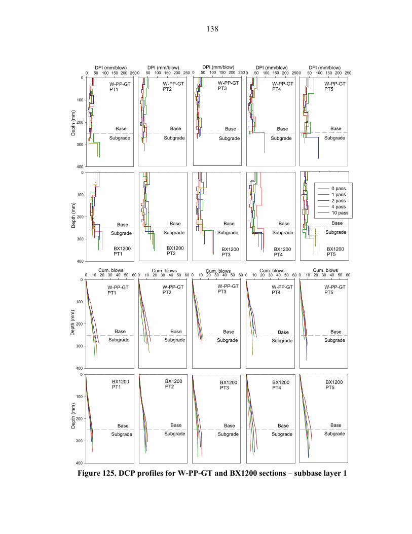
138

Figure 125. DCP profiles for W-PP-GT and BX1200 sections – subbase layer 1

DPI (mm/blow)0 50 100 150 200 250

Dep

th (mm)

0

100

200

300

400

0 pass1 pass2 pass4 pass10 pass

DPI (mm/blow)0 50 100 150 200 250

Cum. blows0 10 20 30 40 50 60

Dep

th (mm)

0

100

200

300

400

Cum. blows0 10 20 30 40 50 60

DPI (mm/blow)0 50 100 150 200 250

DPI (mm/blow)0 50 100 150 200 250

DPI (mm/blow)0 50 100 150 200 250

Dep

th (mm)

0

100

200

300

400

Cum. blows0 10 20 30 40 50 60

Cum. blows0 10 20 30 40 50 60

Cum. blows0 10 20 30 40 50 60

Dep

th (mm)

0

100

200

300

400

Subgrade

Base

Subgrade

Base

Subgrade

Base

Subgrade

Base

Subgrade

Base

Subgrade

Base

Subgrade

Base

Subgrade

Base

Subgrade

Base

Subgrade

Base

Subgrade

Base

Subgrade

Base

Subgrade

Base

Subgrade

Base

Subgrade

Base

Subgrade

Base

Subgrade

Base

Subgrade

Base

Subgrade

Base

Subgrade

Base

W-PP-GTPT1

W-PP-GTPT3

W-PP-GTPT2

W-PP-GTPT5

W-PP-GTPT4

BX1200PT1

BX1200PT2

BX1200PT3

BX1200PT4

BX1200PT5

W-PP-GTPT1

W-PP-GTPT3

W-PP-GTPT2

W-PP-GTPT5

W-PP-GTPT4

BX1200PT1

BX1200PT2

BX1200PT3

BX1200PT4

BX1200PT5

139

Figure 126. DCP profiles for W-PP-GT and BX1200 section – subbase layer 2

DPI (mm/blow)0 50 100 150 200 250

Depth (mm)

0

100

200

300

400

500

600

700

800

900

1000

0 pass1 pass2 pass4 pass10 pass

DPI (mm/blow)0 50 100 150 200 250

Cum. blows0 10 20 30 40 50 60

Depth (mm)

0

100

200

300

400

500

600

700

800

900

1000

Cum. blows0 10 20 30 40 50 60

DPI (mm/blow)0 50 100 150 200 250

DPI (mm/blow)0 50 100 150 200 250

DPI (mm/blow)0 50 100 150 200 250Dep

th (mm)

0

100

200

300

400

500

600

700

800

900

1000

Cum. blows0 10 20 30 40 50 60

Cum. blows0 10 20 30 40 50 60

Cum. blows0 10 20 30 40 50 60

Dep

th (mm)

0

100

200

300

400

500

600

700

800

900

1000

Subgrade

Base 1

Base 2

Subgrade

Base 1

Base 2

Subgrade

Base 1

Base 2

Subgrade

Base 1

Base 2

Subgrade

Base 1

Base 2

Subgrade

Base 1

Base 2

Subgrade

Base 1

Base 2

Subgrade

Base 1

Base 2

Subgrade

Base 1

Base 2

Subgrade

Base 1

Base 2

Subgrade

Base 1

Base 2

Subgrade

Base 1

Base 2

Subgrade

Base 1

Base 2

Subgrade

Base 1

Base 2

Subgrade

Base 1

Base 2

Subgrade

Base 1

Base 2

Subgrade

Base 1

Base 2

Subgrade

Base 1

Base 2

Subgrade

Base 1

Base 2

Subgrade

Base 1

Base 2

W-PP-GTPT1

W-PP-GTPT3

W-PP-GTPT2

W-PP-GTPT5

W-PP-GTPT4

BX1200PT1

BX1200PT2

BX1200PT3

BX1200PT4

BX1200PT5

W-PP-GTPT1

W-PP-GTPT3

W-PP-GTPT2

W-PP-GTPT5

W-PP-GTPT4

BX1200PT1

BX1200PT2

BX1200PT3

BX1200PT4

BX1200PT5

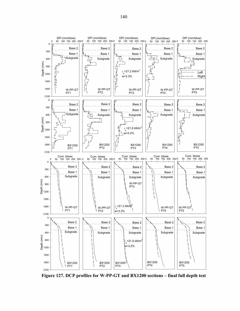
140

Figure 127. DCP profiles for W-PP-GT and BX1200 sections – final full depth test

DPI (mm/blow)0 50 100 150 200 250

Dep

th (mm)

0

300

600

900

1200

1500

1800

2100

LeftRight

DPI (mm/blow)0 50 100 150 200 250

Cum. blows0 50 100 150 200 250

Dep

th (mm)

0

300

600

900

1200

1500

1800

2100

Cum. blows0 50 100 150 200 250

DPI (mm/blow)0 50 100 150 200 250

DPI (mm/blow)0 50 100 150 200 250

DPI (mm/blow)0 50 100 150 200 250Dep

th (mm)

0

300

600

900

1200

1500

1800

2100

Cum. blows0 50 100 150 200 250

Cum. blows0 50 100 150 200 250

Cum. blows0 50 100 150 200 250

Dep

th (mm)

0

300

600

900

1200

1500

1800

2100

γd=21.2 kN/m3

w=3.3%

γd=21.6 kN/m3

w=3.2%

γd=21.2 kN/m3

w=3.3%

γd=21.6 kN/m3

w=3.2%

W-PP-GTPT1

W-PP-GTPT3

W-PP-GTPT2

W-PP-GTPT5

W-PP-GTPT4

BX1200PT1

BX1200PT2

BX1200PT3

BX1200PT4

BX1200PT5

W-PP-GTPT1

W-PP-GTPT3

W-PP-GTPT2

W-PP-GTPT5

W-PP-GTPT4

BX1200PT1

BX1200PT2

BX1200PT3

BX1200PT4

BX1200PT5

Subgrade

Base 1

Base 2

Subgrade

Base 1

Base 2

Subgrade

Base 1

Base 2

Subgrade

Base 1

Base 2

Subgrade

Base 1

Base 2

Subgrade

Base 1

Base 2

Subgrade

Base 1

Base 2

Subgrade

Base 1

Base 2

Subgrade

Base 1

Base 2

Subgrade

Base 1

Base 2

Subgrade

Base 1

Base 2

Subgrade

Base 1

Base 2

Subgrade

Base 1

Base 2

Subgrade

Base 1

Base 2

Subgrade

Base 1

Base 2

Subgrade

Base 1

Base 2

Subgrade

Base 1

Base 2

Subgrade

Base 1

Base 2

Subgrade

Base 1

Base 2

Subgrade

Base 1

Base 2

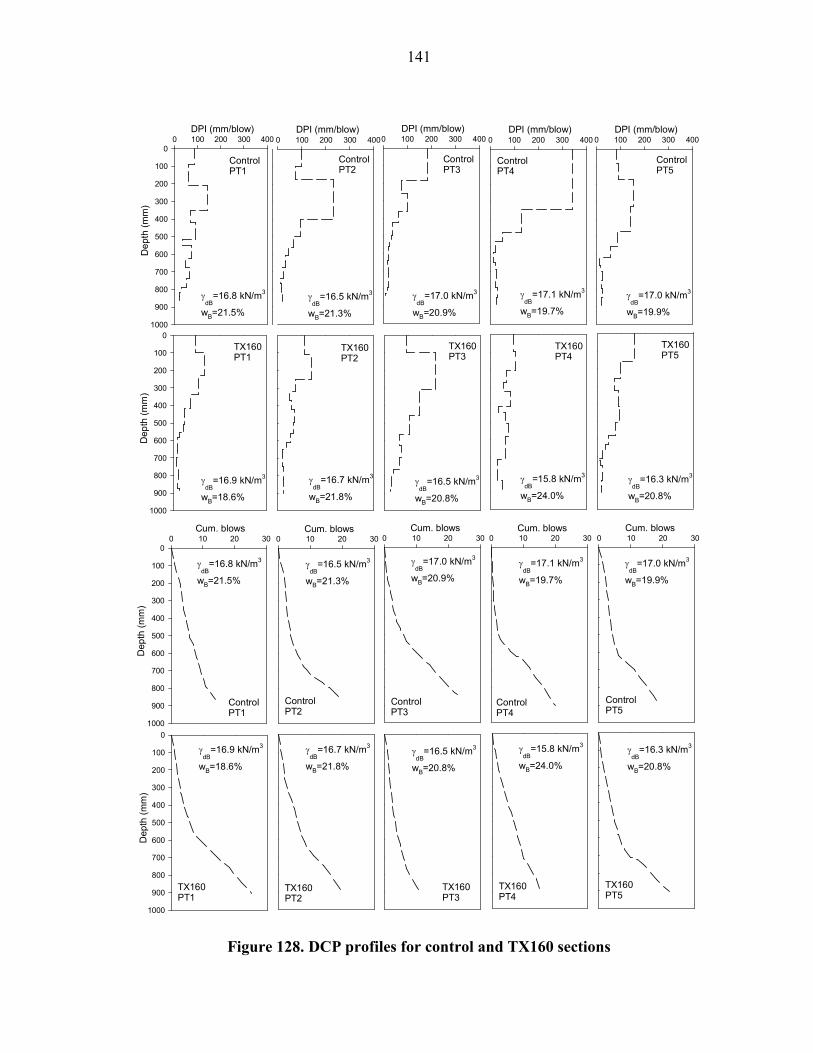
141

Figure 128. DCP profiles for control and TX160 sections

DPI (mm/blow)0 100 200 300 400

Dep

th (mm)

0

100

200

300

400

500

600

700

800

900

1000

DPI (mm/blow)0 100 200 300 400

Cum. blows0 10 20 30

Dep

th (mm)

0

100

200

300

400

500

600

700

800

900

1000

Cum. blows0 10 20 30

DPI (mm/blow)0 100 200 300 400

ControlPT1

ControlPT2

ControlPT3

DPI (mm/blow)0 100 200 300 400

ControlPT4

DPI (mm/blow)0 100 200 300 400

ControlPT5

Dep

th (mm)

0

100

200

300

400

500

600

700

800

900

1000

TX160PT1

TX160PT2

TX160PT3

TX160PT4

TX160PT5

Cum. blows0 10 20 30

Cum. blows0 10 20 30

Cum. blows0 10 20 30

Depth (mm)

0

100

200

300

400

500

600

700

800

900

1000

γdB=16.8 kN/m3

wB=21.5%

γdB=16.5 kN/m3

wB=21.3%

γdB=17.0 kN/m3

wB=20.9%

γdB=17.1 kN/m3

wB=19.7%

γdB=17.0 kN/m3

wB=19.9%

γdB=16.9 kN/m3

wB=18.6%

γdB=16.7 kN/m3

wB=21.8%

γdB=16.5 kN/m3

wB=20.8%

γdB=15.8 kN/m3

wB=24.0%

γdB=16.3 kN/m3

wB=20.8%

γdB=16.8 kN/m3

wB=21.5%

γdB=16.5 kN/m3

wB=21.3%

γdB=17.0 kN/m3

wB=20.9%

γdB=17.1 kN/m3

wB=19.7%

γdB=17.0 kN/m3

wB=19.9%

γdB=16.9 kN/m3

wB=18.6%

γdB=16.7 kN/m3

wB=21.8%

γdB=16.5 kN/m3

wB=20.8%

γdB=15.8 kN/m3

wB=24.0%

γdB=16.3 kN/m3

wB=20.8%

ControlPT1

ControlPT2

ControlPT3

ControlPT4

ControlPT5

TX160PT1

TX160PT2

TX160PT3

TX160PT4

TX160PT5

142

Figure 129. DCP profiles for control and TX160 sections – subbase layer 1

DPI (mm/blow)0 50 100 150 200 250

Depth (mm)

0

100

200

300

400

500

600

0 pass1 pass2 pass4 pass10 pass

DPI (mm/blow)0 50 100 150 200 250

Cum. blows0 10 20 30 40 50 60

Depth (mm)

0

100

200

300

400

500

600

Cum. blows0 10 20 30 40 50 60

DPI (mm/blow)0 50 100 150 200 250

DPI (mm/blow)0 50 100 150 200 250

DPI (mm/blow)0 50 100 150 200 250Dep

th (mm)

0

100

200

300

400

500

600

Cum. blows0 10 20 30 40 50 60

Cum. blows0 10 20 30 40 50 60

Cum. blows0 10 20 30 40 50 60

Depth (mm)

0

100

200

300

400

500

600

Subgrade

Base

Subgrade

Base

Subgrade

Base

Subgrade

Base

Subgrade

Base

Subgrade

Base

Subgrade

Base

Subgrade

Base

Subgrade

Base

Subgrade

Base

Subgrade

Base

Subgrade

Base

Subgrade

Base

Subgrade

Base

Subgrade

Base

Subgrade

BaseSubgrade

Base

Subgrade

Base

Subgrade

BaseSubgrade

Base

ControlPT1

ControlPT2

ControlPT3

ControlPT4

ControlPT5

TX160PT1

TX160PT2

TX160PT3

TX160PT4

TX160PT5

ControlPT1

ControlPT2

ControlPT3

ControlPT4

ControlPT5

TX160PT1

TX160PT2

TX160PT3

TX160PT4

TX160PT5

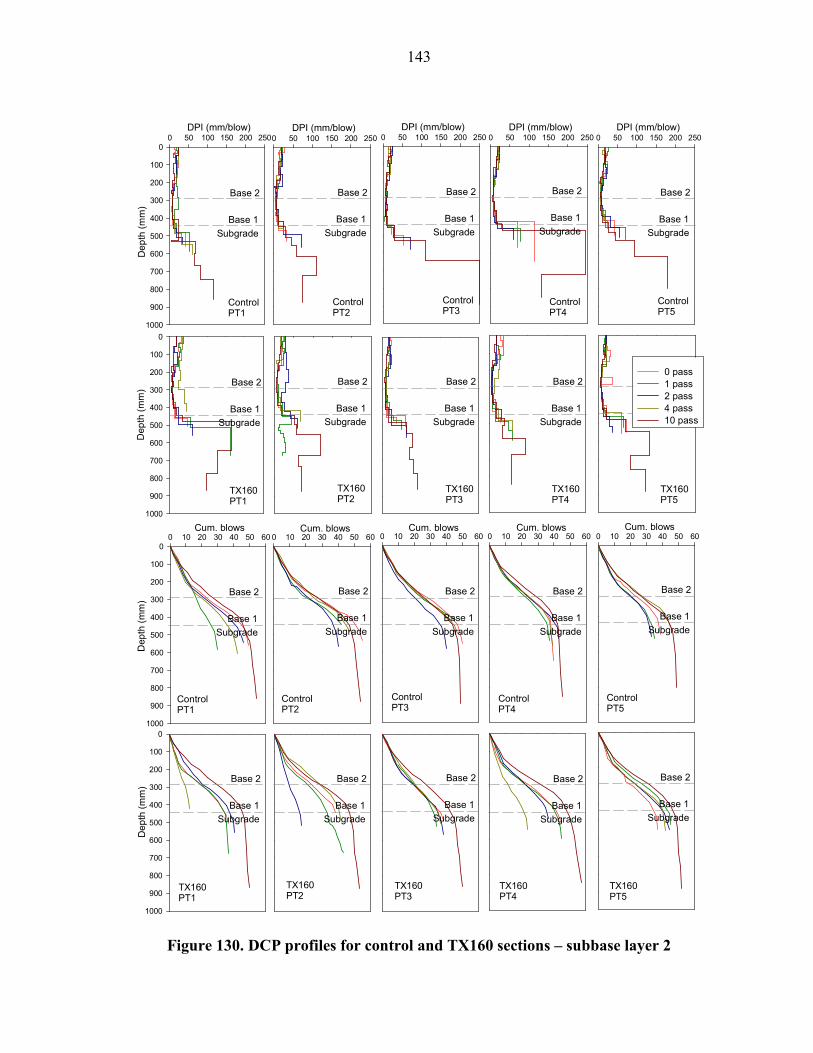
143

Figure 130. DCP profiles for control and TX160 sections – subbase layer 2

DPI (mm/blow)0 50 100 150 200 250

Dep

th (mm)

0

100

200

300

400

500

600

700

800

900

1000

0 pass1 pass2 pass4 pass10 pass

DPI (mm/blow)0 50 100 150 200 250

Cum. blows0 10 20 30 40 50 60

Dep

th (mm)

0

100

200

300

400

500

600

700

800

900

1000

Cum. blows0 10 20 30 40 50 60

DPI (mm/blow)0 50 100 150 200 250

DPI (mm/blow)0 50 100 150 200 250

DPI (mm/blow)0 50 100 150 200 250

Dep

th (mm)

0

100

200

300

400

500

600

700

800

900

1000

Cum. blows0 10 20 30 40 50 60

Cum. blows0 10 20 30 40 50 60

Cum. blows0 10 20 30 40 50 60

Dep

th (mm)

0

100

200

300

400

500

600

700

800

900

1000

SubgradeBase 1

Base 2

SubgradeBase 1

Base 2

SubgradeBase 1

Base 2

SubgradeBase 1

Base 2

SubgradeBase 1

Base 2

SubgradeBase 1

Base 2

SubgradeBase 1

Base 2

SubgradeBase 1

Base 2

SubgradeBase 1

Base 2

SubgradeBase 1

Base 2

SubgradeBase 1

Base 2

SubgradeBase 1

Base 2

SubgradeBase 1

Base 2

SubgradeBase 1

Base 2

SubgradeBase 1

Base 2

SubgradeBase 1

Base 2

SubgradeBase 1

Base 2

SubgradeBase 1

Base 2

SubgradeBase 1

Base 2

ControlPT1

ControlPT2

ControlPT3

ControlPT4

ControlPT5

TX160PT1

TX160PT2

TX160PT3

TX160PT4

TX160PT5

ControlPT1

ControlPT2

ControlPT3

ControlPT4

ControlPT5

TX160PT1

TX160PT2

TX160PT3

TX160PT4

TX160PT5

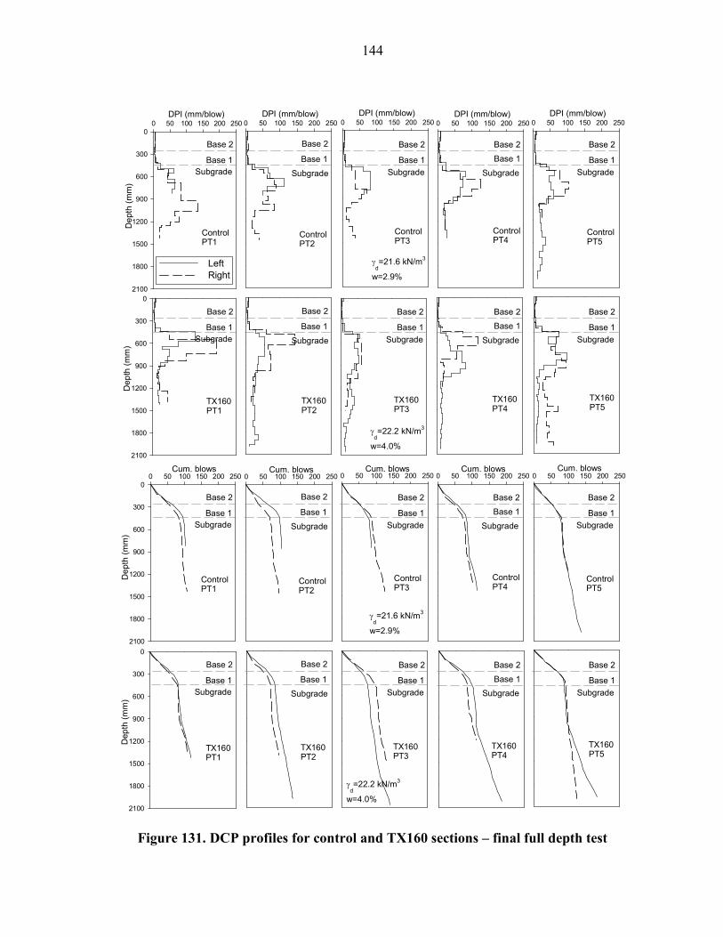
144

Figure 131. DCP profiles for control and TX160 sections – final full depth test

DPI (mm/blow)0 50 100 150 200 250

Dep

th (mm)

0

300

600

900

1200

1500

1800

2100

LeftRight

DPI (mm/blow)0 50 100 150 200 250

Cum. blows0 50 100 150 200 250

Dep

th (mm)

0

300

600

900

1200

1500

1800

2100

Cum. blows0 50 100 150 200 250

DPI (mm/blow)0 50 100 150 200 250

DPI (mm/blow)0 50 100 150 200 250

DPI (mm/blow)0 50 100 150 200 250

Dep

th (mm)

0

300

600

900

1200

1500

1800

2100

Cum. blows0 50 100 150 200 250

Cum. blows0 50 100 150 200 250

Cum. blows0 50 100 150 200 250

Dep

th (mm)

0

300

600

900

1200

1500

1800

2100

γd=21.6 kN/m3

w=2.9%

γd=22.2 kN/m3

w=4.0%

γd=21.6 kN/m3

w=2.9%

γd=22.2 kN/m3

w=4.0%

SubgradeBase 1

Base 2

Subgrade

Base 1

Base 2

SubgradeBase 1

Base 2

Subgrade

Base 1

Base 2

SubgradeBase 1

Base 2

SubgradeBase 1

Base 2

Subgrade

Base 1

Base 2

SubgradeBase 1

Base 2

Subgrade

Base 1

Base 2

SubgradeBase 1

Base 2

SubgradeBase 1

Base 2

Subgrade

Base 1

Base 2

SubgradeBase 1

Base 2

Subgrade

Base 1

Base 2

SubgradeBase 1

Base 2

SubgradeBase 1

Base 2

Subgrade

Base 1

Base 2

SubgradeBase 1

Base 2

Subgrade

Base 1

Base 2

SubgradeBase 1

Base 2

ControlPT1

ControlPT2

ControlPT3

ControlPT4

ControlPT5

TX160PT1

TX160PT2

TX160PT3

TX160PT4

TX160PT5

ControlPT1

ControlPT2

ControlPT3

ControlPT4

ControlPT5

TX160PT1

TX160PT2

TX160PT3

TX160PT4

TX160PT5

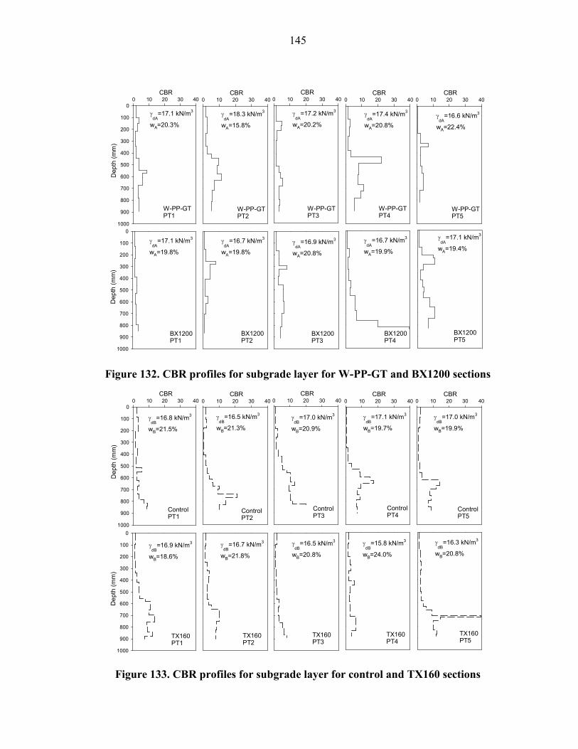
145

Figure 132. CBR profiles for subgrade layer for W-PP-GT and BX1200 sections

Figure 133. CBR profiles for subgrade layer for control and TX160 sections

CBR0 10 20 30 40

Dep

th (mm)

0

100

200

300

400

500

600

700

800

900

1000

CBR0 10 20 30 40

CBR0 10 20 30 40

CBR0 10 20 30 40

CBR0 10 20 30 40

Dep

th (mm)

0

100

200

300

400

500

600

700

800

900

1000

γdA=17.1 kN/m3

wA=20.3%

γdA=18.3 kN/m3

wA=15.8%

γdA=17.2 kN/m3

wA=20.2%

γdA=17.4 kN/m3

wA=20.8%

γdA=16.6 kN/m3

wA=22.4%

γdA=17.1 kN/m3

wA=19.8%

γdA=16.7 kN/m3

wA=19.8%

γdA=16.9 kN/m3

wA=20.8%

γdA=16.7 kN/m3

wA=19.9%

γdA=17.1 kN/m3

wA=19.4%

W-PP-GTPT1

W-PP-GTPT3

W-PP-GTPT2

W-PP-GTPT5

W-PP-GTPT4

BX1200PT1

BX1200PT2

BX1200PT3

BX1200PT4

BX1200PT5

CBR0 10 20 30 40

Dep

th (mm)

0

100

200

300

400

500

600

700

800

900

1000

CBR0 10 20 30 40

CBR0 10 20 30 40

CBR0 10 20 30 40

CBR0 10 20 30 40

Dep

th (mm)

0

100

200

300

400

500

600

700

800

900

1000

γdB=16.8 kN/m3

wB=21.5%

γdB=16.5 kN/m3

wB=21.3%

γdB=17.0 kN/m3

wB=20.9%

γdB=17.1 kN/m3

wB=19.7%

γdB=17.0 kN/m3

wB=19.9%

γdB=16.9 kN/m3

wB=18.6%

γdB=16.7 kN/m3

wB=21.8%

γdB=16.5 kN/m3

wB=20.8%

γdB=15.8 kN/m3

wB=24.0%

γdB=16.3 kN/m3

wB=20.8%

ControlPT1

ControlPT2

ControlPT3

ControlPT4

ControlPT5

TX160PT1

TX160PT2

TX160PT3

TX160PT4

TX160PT5

146

Figure 134. CBR profiles for W-PP-GT and BX1200 sections – subbase layer 1

Figure 135. CBR profiles for W-PP-GT and BX1200 sections – subbase layer 2

CBR0 10 20 30 40 50 60

Dep

th (mm)

0

100

200

300

400

0 pass1 pass2 pass4 pass10 pass

CBR0 10 20 30 40 50 60

CBR0 10 20 30 40 50 60

CBR0 10 20 30 40 50 60

CBR0 10 20 30 40 50 60

Dep

th (mm)

0

100

200

300

400

Subgrade

Base

Subgrade

Base

Subgrade

Base

Subgrade

Base

Subgrade

Base

Subgrade

Base

Subgrade

Base

Subgrade

Base

Subgrade

Base

Subgrade

Base

W-PP-GTPT1

W-PP-GTPT3

W-PP-GTPT2

W-PP-GTPT5

W-PP-GTPT4

BX1200PT1

BX1200PT2

BX1200PT3

BX1200PT4

BX1200PT5

CBR0 10 20 30 40 50 60

Dep

th (mm)

0

100

200

300

400

500

600

700

800

900

1000

0 pass1 pass2 pass4 pass10 pass

CBR0 10 20 30 40 50 60

CBR0 10 20 30 40 50 60

CBR0 10 20 30 40 50 60

CBR0 10 20 30 40 50 60

Dep

th (mm)

0

100

200

300

400

500

600

700

800

900

1000

W-PP-GTPT1

W-PP-GTPT3

W-PP-GTPT2

W-PP-GTPT5

W-PP-GTPT4

BX1200PT1

BX1200PT2

BX1200PT3

BX1200PT4

BX1200PT5

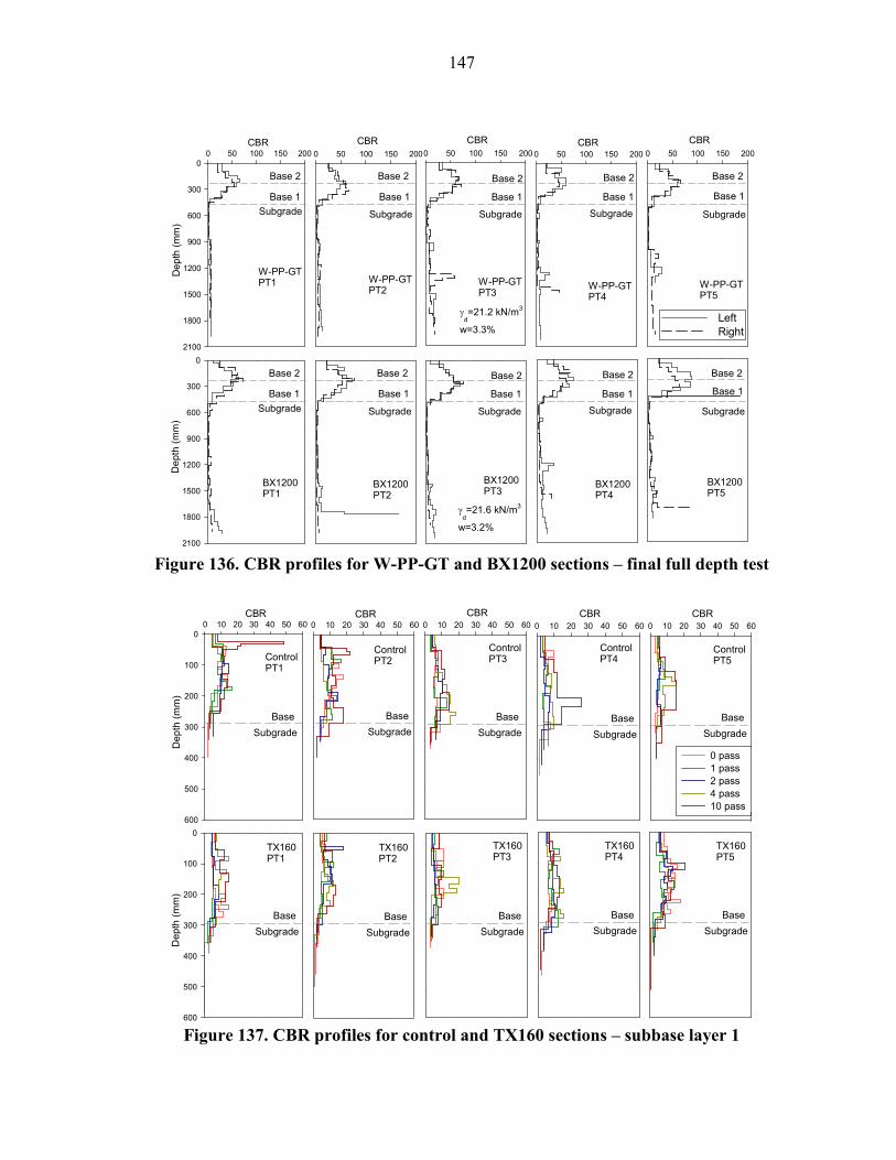
147

Figure 136. CBR profiles for W-PP-GT and BX1200 sections – final full depth test

Figure 137. CBR profiles for control and TX160 sections – subbase layer 1

CBR0 50 100 150 200

Dep

th (mm)

0

300

600

900

1200

1500

1800

2100

LeftRight

CBR0 50 100 150 200

CBR0 50 100 150 200

CBR0 50 100 150 200

CBR0 50 100 150 200

Dep

th (mm)

0

300

600

900

1200

1500

1800

2100

γd=21.2 kN/m3

w=3.3%

γd=21.6 kN/m3

w=3.2%

W-PP-GTPT1 W-PP-GT

PT3W-PP-GTPT2 W-PP-GT

PT5W-PP-GTPT4

BX1200PT1

BX1200PT2

BX1200PT3

BX1200PT4

BX1200PT5

SubgradeBase 1

Base 2

Subgrade

Base 1

Base 2

Subgrade

Base 1

Base 2

Subgrade

Base 1

Base 2

Subgrade

Base 1

Base 2

SubgradeBase 1

Base 2

Subgrade

Base 1

Base 2

Subgrade

Base 1

Base 2

Subgrade

Base 1

Base 2

Subgrade

Base 1

Base 2

CBR0 10 20 30 40 50 60

Dep

th (mm)

0

100

200

300

400

500

600

0 pass1 pass2 pass4 pass10 pass

CBR0 10 20 30 40 50 60

CBR0 10 20 30 40 50 60

CBR0 10 20 30 40 50 60

CBR0 10 20 30 40 50 60

Depth (mm)

0

100

200

300

400

500

600

Subgrade

Base

Subgrade

Base

Subgrade

Base

Subgrade

Base

Subgrade

Base

Subgrade

Base

Subgrade

Base

Subgrade

Base

Subgrade

Base

Subgrade

Base

ControlPT1

ControlPT2

ControlPT3

ControlPT4

ControlPT5

TX160PT1

TX160PT2

TX160PT3

TX160PT4

TX160PT5

148

Figure 138. CBR profiles for control and TX160 sections – subbase layer 2

Figure 139. CBR profiles for control and TX160 sections – final full depth test

CBR0 10 20 30 40 50 60

Dep

th (mm)

0

100

200

300

400

500

600

700

800

900

1000

0 pass1 pass2 pass4 pass10 pass

CBR0 20 40 60 80 100120140

CBR0 10 20 30 40 50 60

CBR0 10 20 30 40 50 60

CBR0 10 20 30 40 50 60

Depth (mm)

0

100

200

300

400

500

600

700

800

900

1000

ControlPT1

ControlPT2

ControlPT3

ControlPT4

ControlPT5

TX160PT1

TX160PT2

TX160PT3

TX160PT4

TX160PT5

CBR0 50 100 150 200

Dep

th (mm)

0

300

600

900

1200

1500

1800

2100

LeftRight

CBR0 50 100 150 200

CBR0 50 100 150 200

CBR0 50 100 150 200

CBR0 50 100 150 200

Dep

th (mm)

0

300

600

900

1200

1500

1800

2100

γd=21.6 kN/m3

w=2.9%

γd=22.2 kN/m3

w=4.0%

ControlPT1

ControlPT2

ControlPT3

ControlPT4

ControlPT5

TX160PT1

TX160PT2

TX160PT3

TX160PT4

TX160PT5

SubgradeBase 1

Base 2

Subgrade

Base 1

Base 2

SubgradeBase 1

Base 2

Subgrade

Base 1

Base 2

SubgradeBase 1

Base 2

SubgradeBase 1

Base 2

Subgrade

Base 1

Base 2

SubgradeBase 1

Base 2

Subgrade

Base 1

Base 2

SubgradeBase 1

Base 2

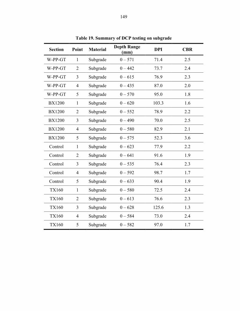
149

Table 19. Summary of DCP testing on subgrade

Section Point Material Depth Range (mm) DPI CBR

W-PP-GT 1 Subgrade 0 – 571 71.4 2.5

W-PP-GT 2 Subgrade 0 – 442 73.7 2.4

W-PP-GT 3 Subgrade 0 – 615 76.9 2.3

W-PP-GT 4 Subgrade 0 – 435 87.0 2.0

W-PP-GT 5 Subgrade 0 – 570 95.0 1.8

BX1200 1 Subgrade 0 – 620 103.3 1.6

BX1200 2 Subgrade 0 – 552 78.9 2.2

BX1200 3 Subgrade 0 – 490 70.0 2.5

BX1200 4 Subgrade 0 – 580 82.9 2.1

BX1200 5 Subgrade 0 – 575 52.3 3.6

Control 1 Subgrade 0 – 623 77.9 2.2

Control 2 Subgrade 0 – 641 91.6 1.9

Control 3 Subgrade 0 – 535 76.4 2.3

Control 4 Subgrade 0 – 592 98.7 1.7

Control 5 Subgrade 0 – 633 90.4 1.9

TX160 1 Subgrade 0 – 580 72.5 2.4

TX160 2 Subgrade 0 – 613 76.6 2.3

TX160 3 Subgrade 0 – 628 125.6 1.3

TX160 4 Subgrade 0 – 584 73.0 2.4

TX160 5 Subgrade 0 – 582 97.0 1.7

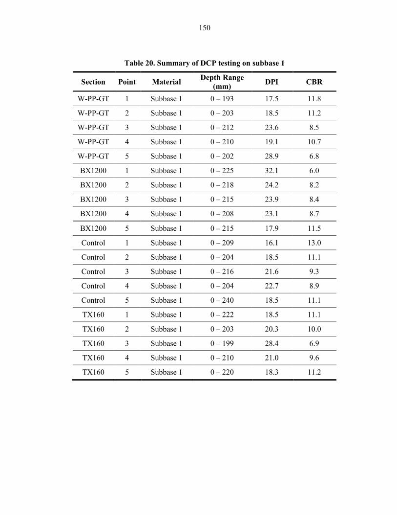
150

Table 20. Summary of DCP testing on subbase 1

Section Point Material Depth Range (mm) DPI CBR

W-PP-GT 1 Subbase 1 0 – 193 17.5 11.8

W-PP-GT 2 Subbase 1 0 – 203 18.5 11.2

W-PP-GT 3 Subbase 1 0 – 212 23.6 8.5

W-PP-GT 4 Subbase 1 0 – 210 19.1 10.7

W-PP-GT 5 Subbase 1 0 – 202 28.9 6.8

BX1200 1 Subbase 1 0 – 225 32.1 6.0

BX1200 2 Subbase 1 0 – 218 24.2 8.2

BX1200 3 Subbase 1 0 – 215 23.9 8.4

BX1200 4 Subbase 1 0 – 208 23.1 8.7

BX1200 5 Subbase 1 0 – 215 17.9 11.5

Control 1 Subbase 1 0 – 209 16.1 13.0

Control 2 Subbase 1 0 – 204 18.5 11.1

Control 3 Subbase 1 0 – 216 21.6 9.3

Control 4 Subbase 1 0 – 204 22.7 8.9

Control 5 Subbase 1 0 – 240 18.5 11.1

TX160 1 Subbase 1 0 – 222 18.5 11.1

TX160 2 Subbase 1 0 – 203 20.3 10.0

TX160 3 Subbase 1 0 – 199 28.4 6.9

TX160 4 Subbase 1 0 – 210 21.0 9.6

TX160 5 Subbase 1 0 – 220 18.3 11.2

151

Table 21. Summary of DCP testing on TB-A after trafficking subbase 2

Section Point Material Depth Range (mm) DPI CBR

W-PP-GT 1L Subbase1 Subgrade

0 – 409 409 – 875

5.8 77.7

41.1 2.2

W-PP-GT 1R Subbase1 Subgrade

0 – 389 448 – 846

6.7 99.5

34.6 1.7

W-PP-GT 2L Subbase1 Subgrade

0 – 404 480 – 874

6.1 65.7

38.4 2.7

W-PP-GT 2R Subbase1 Subgrade

0 – 419 499 – 854

5.3 71.0

45.1 2.5

W-PP-GT 3L Subbase1 Subgrade

0 – 403 515 – 821

5.0 76.5

48.4 2.3

W-PP-GT 3R Subbase1 Subgrade

0 – 416 497 – 767

5.0 45.0

48.0 4.1

W-PP-GT 4L Subbase1 Subgrade

0 – 361 466 – 824

5.6 71.6

42.8 2.4

W-PP-GT 4R Subbase1 Subgrade

0 – 331 529 – 887

6.6 71.6

35.2 2.4

W-PP-GT 5L Subbase1 Subgrade

0 – 369 496 – 933

5.7 109.3

41.8 1.5

W-PP-GT 5R Subbase1 Subgrade

0 – 389 513 – 864

5.6 87.8

42.8 1.9

BX1200 1L Subbase1 Subgrade

0 – 367 497 – 932

5.8 108.8

40.6 1.5

BX1200 1R Subbase1 Subgrade

0 – 408 574 – 958

5.1 48.0

47.1 3.8

BX1200 2L Subbase1 Subgrade

0 – 375 437 – 907

4.7 67.1

51.8 2.6

BX1200 2R Subbase1 Subgrade

0 – 401 574 – 885

5.7 103.7

41.3 1.6

BX1200 3L Subbase1 Subgrade

0 – 383 478 – 865

5.3 96.8

44.9 1.7

BX1200 3R Subbase1 Subgrade

0 – 365 641 – 982

5.2 85.3

45.9 2.0

BX1200 4L Subbase1 Subgrade

0 – 429 511 – 906

5.0 39.5

47.6 4.8

BX1200 4R Subbase1 Subgrade

0 – 413 490 – 851

5.3 72.2

45.2 2.4

BX1200 5L Subbase1 Subgrade

0 – 363 421 – 844

3.8 84.6

65.1 2.0

BX1200 5R Subbase1 Subgrade

0 – 434 484 – 963

5.4 59.9

43.9 3.0

1 Subbase includes subbase 1 and subbase 2 as included in depth ranges.

152

Table 22. Summary of DCP testing on TB-B after trafficking subbase 2

Section Point Material Depth Range (mm) DPI CBR

Control 1L Subbase1 Subgrade

0 – 421 489 – 824

4.4 55.8

55.1 3.2

Control 1R Subbase1 Subgrade

0 – 405 503 – 927

5.1 60.6

47.5 2.9

Control 2L Subbase1 Subgrade

0 – 442 493 – 855

4.6 51.7

53.4 3.5

Control 2R Subbase1 Subgrade

0 – 443 512 – 930

6.4 69.7

36.4 2.5

Control 3L Subbase1 Subgrade

0 – 485 485 – 854

6.1 73.8

38.8 2.4

Control 3R Subbase1 Subgrade

0 – 407 534 – 957

5.1 42.3

47.2 4.4

Control 4L Subbase1 Subgrade

0 – 414 528 – 967

5.2 62.7

46.3 2.8

Control 4R Subbase1 Subgrade

0 – 410 516 – 924

5.9 81.6

40.3 2.1

Control 5L Subbase1 Subgrade

0 – 430 488 – 907

5.7 52.4

41.3 3.5

Control 5R Subbase1 Subgrade

0 – 450 529 – 876

5.6 86.8

42.2 2.0

TX160 1L Subbase1 Subgrade

0 – 389 439 – 911

4.9 52.4

49.7 3.5

TX160 1R Subbase1 Subgrade

0 – 442 542 – 906

5.5 91.0

43.0 1.9

TX160 2L Subbase1 Subgrade

0 – 338 516 – 896

4.5 47.5

54.1 3.9

TX160 2R Subbase1 Subgrade

0 – 423 483 – 978

6.0 82.5

38.9 2.1

TX160 3L Subbase1 Subgrade

0 – 335 484 – 875

5.2 48.9

46.5 3.7

TX160 3R Subbase1 Subgrade

0 – 482 482 – 888

4.8 58.0

50.2 3.1

TX160 4L Subbase1 Subgrade

0 – 376 572 – 952

4.2 54.3

58.9 3.3

TX160 4R Subbase1 Subgrade

0 – 392 454 – 825

4.9 74.2

49.2 2.3

TX160 5L Subbase1 Subgrade

0 – 391 468 – 920

4.6 64.6

52.9 2.7

TX160 5R Subbase1 Subgrade

0 – 416 465 - 956

4.6 70.1

52.6 2.5

1 Subbase includes subbase 1 and subbase 2 as included in depth ranges.

153

Raw Data from the Influence of Layered Soil Profiles on Surface Modulus Study

Soft soil over stiff soil – Data from Ohio Bridge Approach Project Site

Table 23. Raw data for the correlation between Eequivalent and ELWD-Z2 – Ohio Site

PT# Sum (IZ) Sum (CBR××××IZ) CBRequi.

[Sum (CBR××××IZ)/ Sum (IZ)] Eequi. ELWD-Z2

1 12.5 229.0 18.3 113.0 61.9 2 0.03 0.005 0.2 5.9 5.9 3 4.2 69.2 16.6 106.3 17.7 4 7.5 133.0 17.7 110.6 38.1 5 7.9 123.7 15.6 102.0 51.4 6 6.8 101.3 14.9 98.9 52.3 7 14.9 462.5 31.1 158.7 85.7 8 10.6 423.7 40.0 186.2 73.5 9 2.1 7.3 3.5 39.5 8.9

10 5.9 106.7 18.2 112.5 36.1 11 9.3 154.7 16.6 106.3 59.7 12 11.1 221.3 20.0 119.5 68.2 13 3.2 34.6 10.9 80.9 47.3 14 7.2 164.1 22.9 130.3 61.4 15 0.6 5.3 8.8 70.8 8.0 16 16.0 354.8 22.2 127.7 19.6 17 5.9 106.2 17.9 111.3 21.2 18 8.8 164.2 18.7 114.5 27.7 19 13.7 381.6 27.9 148.1 29.5 20 4.6 60.6 13.1 91.3 13.9 21 3.3 18.0 5.4 51.8 8.5 22 0.5 1.1 2.1 28.7 7.5 23 7.5 179.9 23.9 133.9 29.6 24 7.0 183.3 26.3 142.5 28.1 25 5.6 166.1 29.6 153.8 39.8 26 4.1 65.0 15.7 102.5 22.9 27 0.8 1.9 2.5 31.6 7.7 28 3.5 36.5 10.5 79.0 18.6 29 7.6 170.6 22.5 129.1 35.0 30 6.3 89.3 14.1 95.6 26.8 31 2.8 30.9 11.1 81.9 20.4

154

Stiff soil over soft soil – Data from Hormel PCC Project Site

Table 24. Raw data for the correlation between Eequivalent and ELWD-Z2 – Dubuque Site

PT# Sum (IZ) Sum (CBR××××IZ) CBRequi.

[Sum (CBR××××IZ)/ Sum (IZ)] Eequi. ELWD-Z2

1 25.7 1407.0 54.8 227.9 40.2 2 11.5 238.6 20.7 122.3 20.0 3 22.6 989.0 43.8 197.6 24.6 4 10.1 172.2 17.0 107.9 14.7 5 23.1 1176.5 51.0 217.6 25.6 6 4.2 24.7 5.9 54.6 13.7 7 7.7 122.5 15.8 103.0 16.2 8 5.7 54.2 9.5 74.1 13.3 9 12.6 272.0 21.6 125.5 21.2

10 9.2 443.7 48.1 209.6 30.6 11 5.2 83.9 16.1 104.0 17.6 12 10.2 312.8 30.7 157.2 25.2 13 18.1 905.9 49.9 214.8 85.1 14 7.6 130.8 17.1 108.3 15.0 15 8.7 240.2 27.5 146.7 19.3 16 12.5 526.3 42.1 192.6 46.9 17 11.1 294.1 26.6 143.4 37.0 18 10.9 355.4 32.7 163.7 32.3 19 14.1 523.8 37.2 177.8 36.6 20 13.1 294.3 22.5 129.0 17.7 21 17.8 546.0 30.6 157.1 30.0 22 13.6 345.7 25.5 139.6 18.9 23 14.9 418.7 28.1 148.6 19.7 24 17.0 551.5 32.5 163.3 27.2 25 17.1 527.8 30.8 157.7 23.7 26 11.3 220.4 19.4 117.4 19.1 27 16.7 517.7 31.0 158.3 37.2 28 23.9 1242.6 52.1 220.6 50.1 29 8.1 109.8 13.5 93.2 17.1 30 9.7 179.1 18.5 113.7 21.0 31 7.0 92.9 13.3 92.3 13.3 32 8.2 120.3 14.7 98.3 13.0 33 2.7 10.8 4.0 42.9 9.3 34 3.9 26.9 6.8 60.2 12.6 35 16.9 666.0 39.4 184.5 45.6 36 10.0 397.1 39.9 186.0 40.4 37 7.4 86.9 11.7 84.8 16.3 38 9.3 153.6 16.5 105.7 19.6 39 7.0 154.4 22.0 127.2 20.2 40 12.9 336.5 26.1 141.7 18.9 41 4.4 27.9 6.4 57.5 8.3 42 8.5 127.2 15.1 99.7 18.7

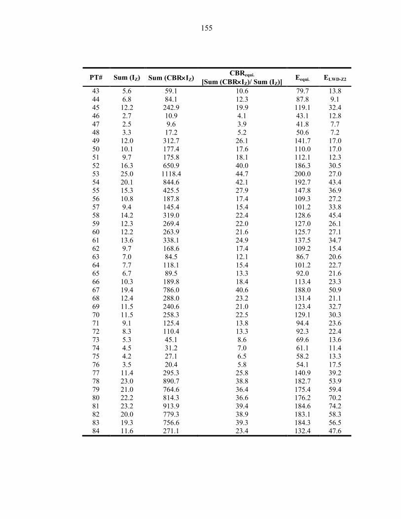
155

PT# Sum (IZ) Sum (CBR××××IZ) CBRequi.

[Sum (CBR××××IZ)/ Sum (IZ)] Eequi. ELWD-Z2

43 5.6 59.1 10.6 79.7 13.8 44 6.8 84.1 12.3 87.8 9.1 45 12.2 242.9 19.9 119.1 32.4 46 2.7 10.9 4.1 43.1 12.8 47 2.5 9.6 3.9 41.8 7.7 48 3.3 17.2 5.2 50.6 7.2 49 12.0 312.7 26.1 141.7 17.0 50 10.1 177.4 17.6 110.0 17.0 51 9.7 175.8 18.1 112.1 12.3 52 16.3 650.9 40.0 186.3 30.5 53 25.0 1118.4 44.7 200.0 27.0 54 20.1 844.6 42.1 192.7 43.4 55 15.3 425.5 27.9 147.8 36.9 56 10.8 187.8 17.4 109.3 27.2 57 9.4 145.4 15.4 101.2 33.8 58 14.2 319.0 22.4 128.6 45.4 59 12.3 269.4 22.0 127.0 26.1 60 12.2 263.9 21.6 125.7 27.1 61 13.6 338.1 24.9 137.5 34.7 62 9.7 168.6 17.4 109.2 15.4 63 7.0 84.5 12.1 86.7 20.6 64 7.7 118.1 15.4 101.2 22.7 65 6.7 89.5 13.3 92.0 21.6 66 10.3 189.8 18.4 113.4 23.3 67 19.4 786.0 40.6 188.0 50.9 68 12.4 288.0 23.2 131.4 21.1 69 11.5 240.6 21.0 123.4 32.7 70 11.5 258.3 22.5 129.1 30.3 71 9.1 125.4 13.8 94.4 23.6 72 8.3 110.4 13.3 92.3 22.4 73 5.3 45.1 8.6 69.6 13.6 74 4.5 31.2 7.0 61.1 11.4 75 4.2 27.1 6.5 58.2 13.3 76 3.5 20.4 5.8 54.1 17.5 77 11.4 295.3 25.8 140.9 39.2 78 23.0 890.7 38.8 182.7 53.9 79 21.0 764.6 36.4 175.4 59.4 80 22.2 814.3 36.6 176.2 70.2 81 23.2 913.9 39.4 184.6 74.2 82 20.0 779.3 38.9 183.1 58.3 83 19.3 756.6 39.3 184.3 56.5 84 11.6 271.1 23.4 132.4 47.6

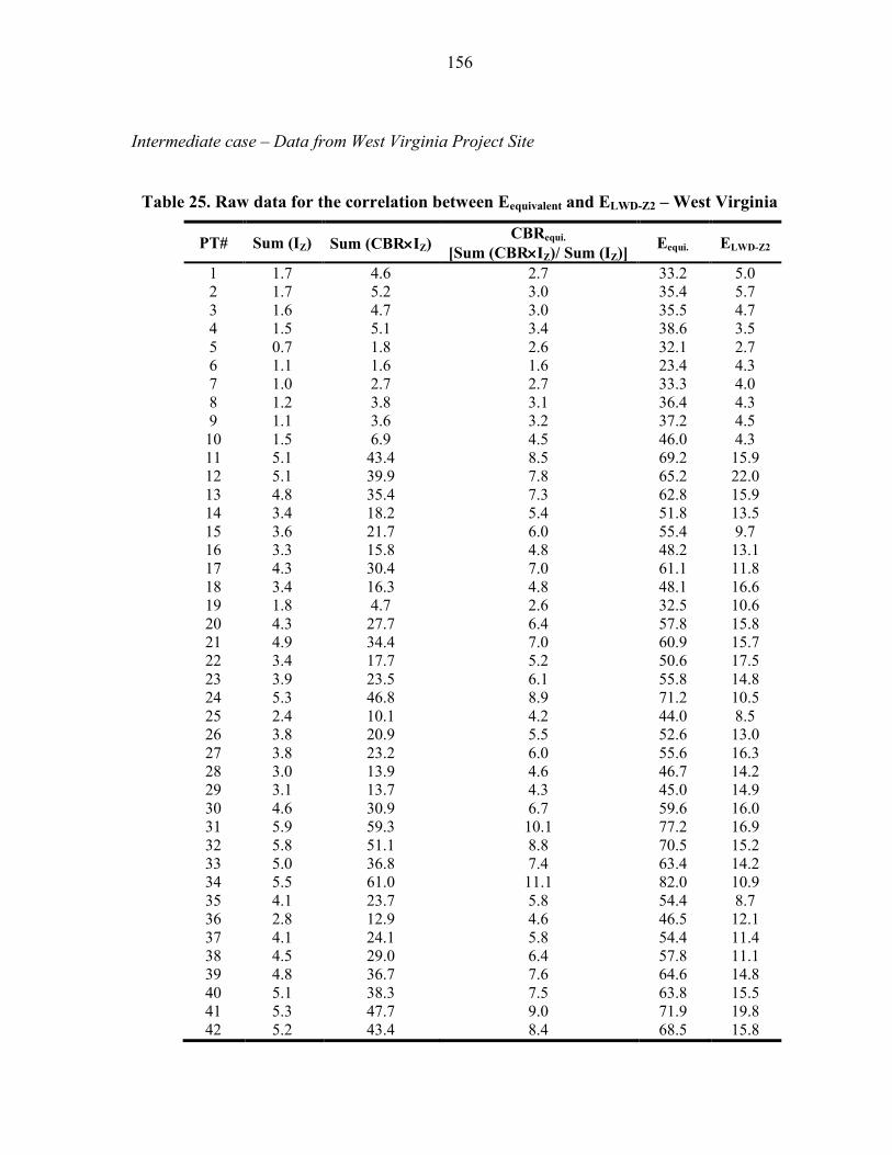
156

Intermediate case – Data from West Virginia Project Site

Table 25. Raw data for the correlation between Eequivalent and ELWD-Z2 – West Virginia

PT# Sum (IZ) Sum (CBR××××IZ) CBRequi.

[Sum (CBR××××IZ)/ Sum (IZ)] Eequi. ELWD-Z2

1 1.7 4.6 2.7 33.2 5.0 2 1.7 5.2 3.0 35.4 5.7 3 1.6 4.7 3.0 35.5 4.7 4 1.5 5.1 3.4 38.6 3.5 5 0.7 1.8 2.6 32.1 2.7 6 1.1 1.6 1.6 23.4 4.3 7 1.0 2.7 2.7 33.3 4.0 8 1.2 3.8 3.1 36.4 4.3 9 1.1 3.6 3.2 37.2 4.5

10 1.5 6.9 4.5 46.0 4.3 11 5.1 43.4 8.5 69.2 15.9 12 5.1 39.9 7.8 65.2 22.0 13 4.8 35.4 7.3 62.8 15.9 14 3.4 18.2 5.4 51.8 13.5 15 3.6 21.7 6.0 55.4 9.7 16 3.3 15.8 4.8 48.2 13.1 17 4.3 30.4 7.0 61.1 11.8 18 3.4 16.3 4.8 48.1 16.6 19 1.8 4.7 2.6 32.5 10.6 20 4.3 27.7 6.4 57.8 15.8 21 4.9 34.4 7.0 60.9 15.7 22 3.4 17.7 5.2 50.6 17.5 23 3.9 23.5 6.1 55.8 14.8 24 5.3 46.8 8.9 71.2 10.5 25 2.4 10.1 4.2 44.0 8.5 26 3.8 20.9 5.5 52.6 13.0 27 3.8 23.2 6.0 55.6 16.3 28 3.0 13.9 4.6 46.7 14.2 29 3.1 13.7 4.3 45.0 14.9 30 4.6 30.9 6.7 59.6 16.0 31 5.9 59.3 10.1 77.2 16.9 32 5.8 51.1 8.8 70.5 15.2 33 5.0 36.8 7.4 63.4 14.2 34 5.5 61.0 11.1 82.0 10.9 35 4.1 23.7 5.8 54.4 8.7 36 2.8 12.9 4.6 46.5 12.1 37 4.1 24.1 5.8 54.4 11.4 38 4.5 29.0 6.4 57.8 11.1 39 4.8 36.7 7.6 64.6 14.8 40 5.1 38.3 7.5 63.8 15.5 41 5.3 47.7 9.0 71.9 19.8 42 5.2 43.4 8.4 68.5 15.8

157

PT# Sum (IZ) Sum (CBR××××IZ) CBRequi.

[Sum (CBR××××IZ)/ Sum (IZ)] Eequi. ELWD-Z2

43 7.1 92.4 12.9 90.5 15.4 44 3.5 17.9 5.1 50.0 10.9 45 4.4 30.1 6.8 59.9 10.0 46 3.9 24.6 6.3 57.2 13.5 47 4.6 31.5 6.9 60.3 12.3 48 3.5 21.8 6.3 57.2 12.9 49 3.9 25.2 6.4 57.7 16.3 50 5.5 45.1 8.2 67.8 13.8 51 7.4 89.7 12.0 86.4 20.8 52 7.4 83.5 11.4 83.3 15.7 53 5.6 48.6 8.7 70.4 15.2 54 6.7 78.4 11.7 84.7 10.9 55 4.5 34.6 7.6 64.6 9.0 56 3.1 18.3 5.9 54.6 12.3 57 4.6 42.7 9.2 72.9 18.8 58 5.4 44.3 8.2 67.4 12.4 59 5.8 52.7 9.1 72.1 16.7 60 7.4 90.5 12.2 87.2 15.5 61 7.9 126.7 16.1 104.1 23.9 62 6.6 81.5 12.3 87.5 31.0 63 6.8 78.7 11.5 84.1 30.9 64 6.9 85.3 12.4 88.2 25.0 65 6.0 58.9 9.9 76.1 26.5 66 5.2 52.7 10.2 77.8 25.9 67 5.8 85.7 14.7 98.2 27.9 68 4.9 50.6 10.4 78.9 27.3 69 5.0 47.2 9.4 73.8 26.2 70 6.5 78.9 12.1 86.6 26.3 71 3.1 34.7 11.2 82.7 20.4 72 3.4 36.3 10.7 80.2 26.3 73 2.9 46.5 15.8 102.9 28.6 74 3.0 44.8 15.2 100.2 21.3 75 3.2 26.8 8.4 68.7 18.9 76 2.7 36.2 13.2 91.6 26.0 77 2.7 23.8 8.7 70.4 23.3 78 2.7 26.2 9.9 76.1 23.0 79 4.0 47.5 11.9 85.7 25.6 80 3.7 46.0 12.5 88.6 23.6 81 5.0 58.4 11.8 85.3 22.4 82 3.5 37.2 10.8 80.5 24.4 83 4.9 79.3 16.2 104.5 25.6 84 3.9 52.7 13.7 93.8 22.2 85 4.3 47.8 11.2 82.6 23.6 86 3.7 38.1 10.3 78.1 20.8 87 3.1 28.4 9.2 72.9 25.2 88 3.8 41.2 10.9 80.9 22.9

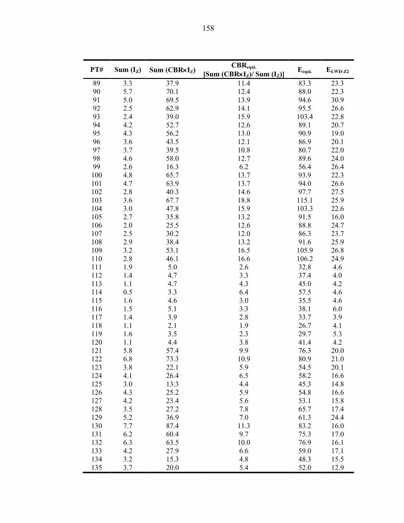
158

PT# Sum (IZ) Sum (CBR××××IZ) CBRequi.

[Sum (CBR××××IZ)/ Sum (IZ)] Eequi. ELWD-Z2

89 3.3 37.9 11.4 83.3 23.3 90 5.7 70.1 12.4 88.0 22.3 91 5.0 69.5 13.9 94.6 30.9 92 2.5 62.9 14.1 95.5 26.6 93 2.4 39.0 15.9 103.4 22.8 94 4.2 52.7 12.6 89.1 20.7 95 4.3 56.2 13.0 90.9 19.0 96 3.6 43.5 12.1 86.9 20.1 97 3.7 39.5 10.8 80.7 22.0 98 4.6 58.0 12.7 89.6 24.0 99 2.6 16.3 6.2 56.4 26.4

100 4.8 65.7 13.7 93.9 22.3 101 4.7 63.9 13.7 94.0 26.6 102 2.8 40.3 14.6 97.7 27.5 103 3.6 67.7 18.8 115.1 25.9 104 3.0 47.8 15.9 103.3 22.6 105 2.7 35.8 13.2 91.5 16.0 106 2.0 25.5 12.6 88.8 24.7 107 2.5 30.2 12.0 86.3 23.7 108 2.9 38.4 13.2 91.6 25.9 109 3.2 53.1 16.5 105.9 26.8 110 2.8 46.1 16.6 106.2 24.9 111 1.9 5.0 2.6 32.8 4.6 112 1.4 4.7 3.3 37.4 4.0 113 1.1 4.7 4.3 45.0 4.2 114 0.5 3.3 6.4 57.5 4.6 115 1.6 4.6 3.0 35.5 4.6 116 1.5 5.1 3.3 38.1 6.0 117 1.4 3.9 2.8 33.7 3.9 118 1.1 2.1 1.9 26.7 4.1 119 1.6 3.5 2.3 29.7 5.3 120 1.1 4.4 3.8 41.4 4.2 121 5.8 57.4 9.9 76.3 20.0 122 6.8 73.3 10.9 80.9 21.0 123 3.8 22.1 5.9 54.5 20.1 124 4.1 26.4 6.5 58.2 16.6 125 3.0 13.3 4.4 45.3 14.8 126 4.3 25.2 5.9 54.8 16.6 127 4.2 23.4 5.6 53.1 15.8 128 3.5 27.2 7.8 65.7 17.4 129 5.2 36.9 7.0 61.3 24.4 130 7.7 87.4 11.3 83.2 16.0 131 6.2 60.4 9.7 75.3 17.0 132 6.3 63.5 10.0 76.9 16.1 133 4.2 27.9 6.6 59.0 17.1 134 3.2 15.3 4.8 48.3 15.5 135 3.7 20.0 5.4 52.0 12.9

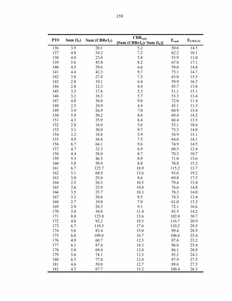
159

PT# Sum (IZ) Sum (CBR××××IZ) CBRequi.

[Sum (CBR××××IZ)/ Sum (IZ)] Eequi. ELWD-Z2

136 3.9 20.1 5.2 50.6 14.5 137 4.8 34.2 7.2 62.2 10.1 138 4.0 23.0 5.8 53.9 11.0 139 5.6 45.8 8.2 67.8 17.1 140 4.5 29.6 6.6 59.0 14.8 141 4.4 42.3 9.7 75.1 14.7 142 3.8 27.8 7.3 63.0 15.5 143 2.8 19.1 6.8 59.9 16.3 144 2.8 12.3 4.4 45.7 13.8 145 3.3 17.6 5.3 51.1 13.1 146 3.2 18.3 5.7 53.3 13.4 147 4.0 36.0 9.0 72.0 11.4 148 2.5 10.9 4.4 45.1 11.5 149 3.9 26.9 7.0 60.9 15.4 150 5.9 50.2 8.6 69.4 14.2 151 4.3 35.9 8.4 68.4 13.5 152 2.8 16.0 5.6 53.1 18.6 153 3.1 30.0 9.7 75.3 14.8 154 3.2 18.8 5.9 54.9 15.1 155 4.9 36.8 7.5 64.0 14.1 156 6.7 64.1 9.6 74.9 14.5 157 4.7 32.3 6.9 60.5 12.4 158 4.4 38.0 8.7 70.3 10.7 159 5.3 46.5 8.9 71.0 15.6 160 5.8 50.9 8.8 70.8 15.2 161 6.7 125.7 18.9 115.2 13.7 162 5.1 68.9 13.6 93.6 19.2 163 3.0 25.6 8.6 69.8 17.5 164 2.5 26.3 10.5 79.4 15.4 165 2.6 25.9 10.0 76.6 14.8 166 3.5 35.7 10.3 78.3 14.0 167 3.2 30.6 9.5 74.5 13.4 168 2.7 19.0 7.0 61.0 13.3 169 2.9 26.5 9.1 72.1 16.6 170 3.4 38.8 11.4 83.5 14.2 171 8.0 125.0 15.6 102.0 30.7 172 4.8 92.2 19.3 116.7 20.9 173 6.7 118.5 17.6 110.2 29.5 174 5.6 83.4 15.0 99.4 28.9 175 6.6 109.6 16.7 106.6 25.4 176 4.9 60.7 12.3 87.6 23.2 177 6.1 87.4 14.3 96.6 25.4 178 5.8 69.4 12.0 86.1 28.0 179 5.6 74.1 13.3 92.2 24.2 180 6.3 77.8 12.4 87.9 27.5 181 4.6 59.0 12.7 89.6 27.5 182 4.5 67.7 15.2 100.4 26.3

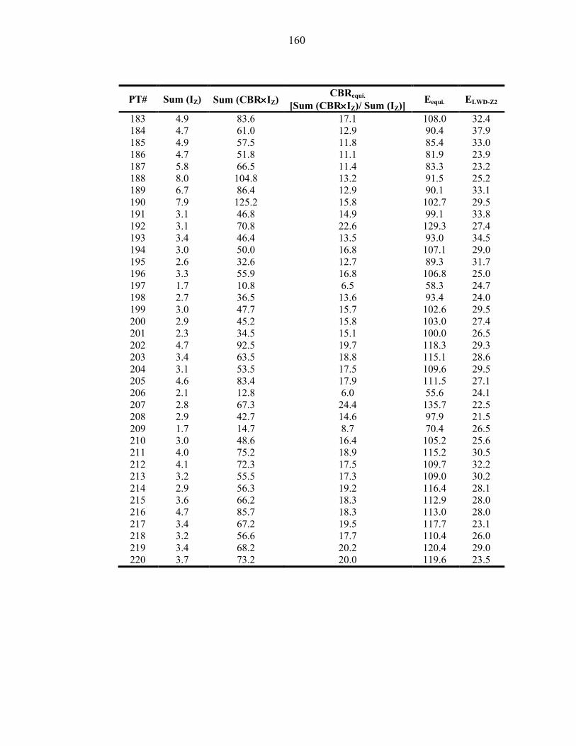
160

PT# Sum (IZ) Sum (CBR××××IZ) CBRequi.

[Sum (CBR××××IZ)/ Sum (IZ)] Eequi. ELWD-Z2

183 4.9 83.6 17.1 108.0 32.4 184 4.7 61.0 12.9 90.4 37.9 185 4.9 57.5 11.8 85.4 33.0 186 4.7 51.8 11.1 81.9 23.9 187 5.8 66.5 11.4 83.3 23.2 188 8.0 104.8 13.2 91.5 25.2 189 6.7 86.4 12.9 90.1 33.1 190 7.9 125.2 15.8 102.7 29.5 191 3.1 46.8 14.9 99.1 33.8 192 3.1 70.8 22.6 129.3 27.4 193 3.4 46.4 13.5 93.0 34.5 194 3.0 50.0 16.8 107.1 29.0 195 2.6 32.6 12.7 89.3 31.7 196 3.3 55.9 16.8 106.8 25.0 197 1.7 10.8 6.5 58.3 24.7 198 2.7 36.5 13.6 93.4 24.0 199 3.0 47.7 15.7 102.6 29.5 200 2.9 45.2 15.8 103.0 27.4 201 2.3 34.5 15.1 100.0 26.5 202 4.7 92.5 19.7 118.3 29.3 203 3.4 63.5 18.8 115.1 28.6 204 3.1 53.5 17.5 109.6 29.5 205 4.6 83.4 17.9 111.5 27.1 206 2.1 12.8 6.0 55.6 24.1 207 2.8 67.3 24.4 135.7 22.5 208 2.9 42.7 14.6 97.9 21.5 209 1.7 14.7 8.7 70.4 26.5 210 3.0 48.6 16.4 105.2 25.6 211 4.0 75.2 18.9 115.2 30.5 212 4.1 72.3 17.5 109.7 32.2 213 3.2 55.5 17.3 109.0 30.2 214 2.9 56.3 19.2 116.4 28.1 215 3.6 66.2 18.3 112.9 28.0 216 4.7 85.7 18.3 113.0 28.0 217 3.4 67.2 19.5 117.7 23.1 218 3.2 56.6 17.7 110.4 26.0 219 3.4 68.2 20.2 120.4 29.0 220 3.7 73.2 20.0 119.6 23.5

161

APPENDIX II: STATISTICAL MODELS

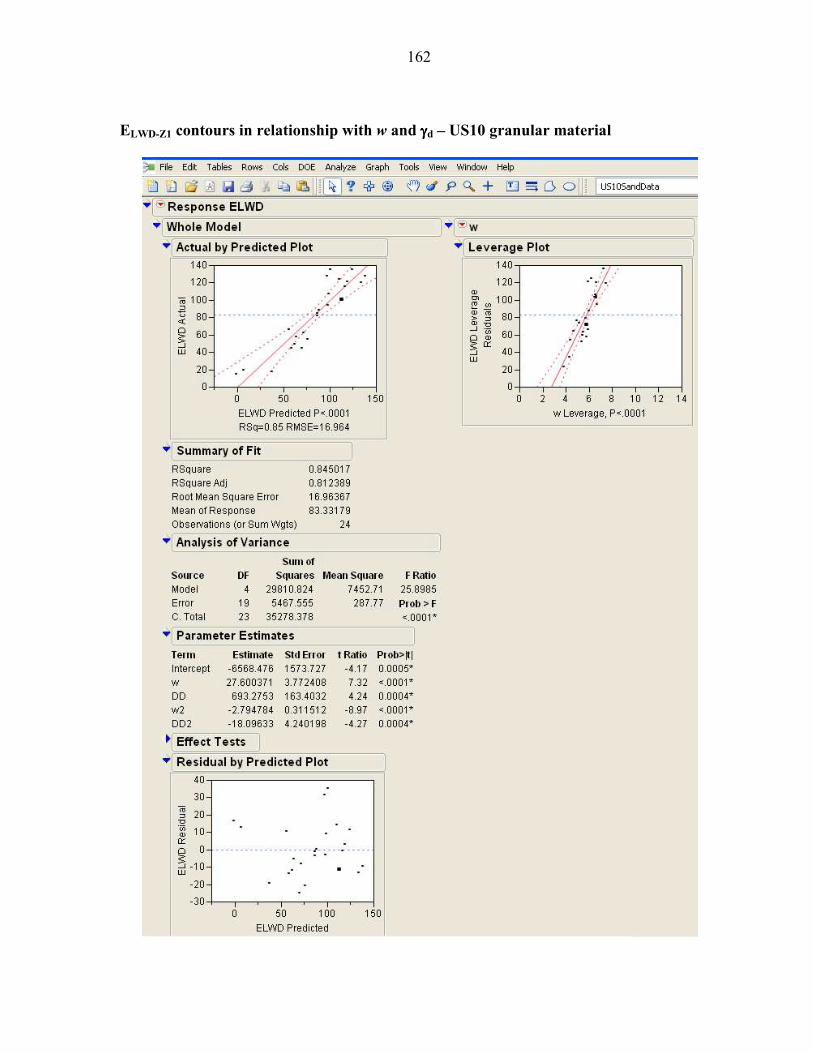
162

ELWD-Z1 contours in relationship with w and γγγγd – US10 granular material

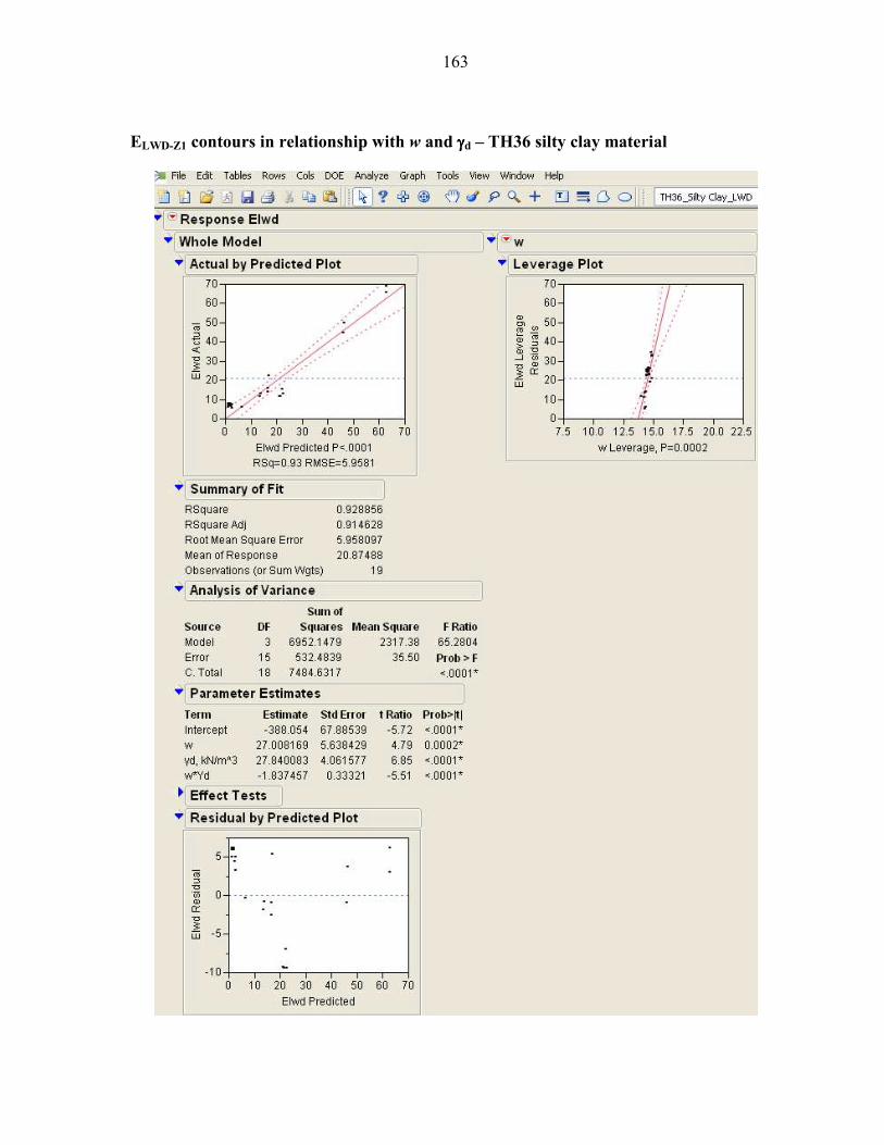
163

ELWD-Z1 contours in relationship with w and γγγγd – TH36 silty clay material

164

ELWD-Z1 contours in relationship with w and γγγγd – TH60 soil 301 material

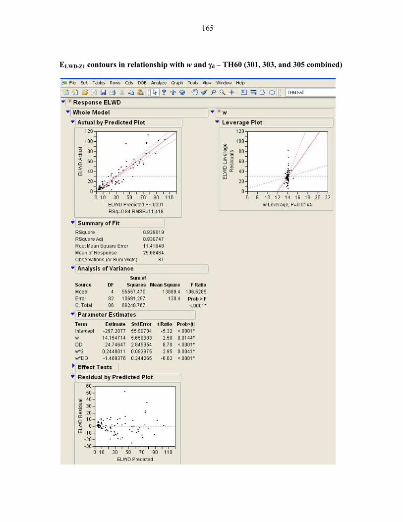
165

ELWD-Z1 contours in relationship with w and γγγγd – TH60 (301, 303, and 305 combined)

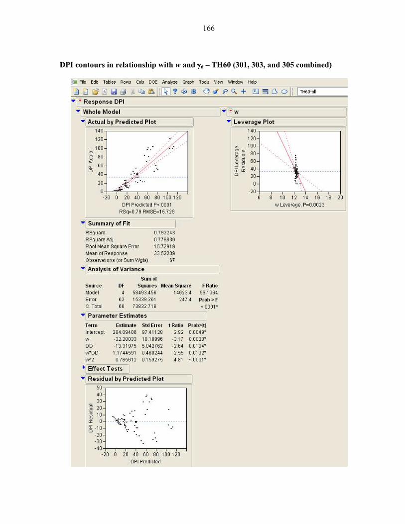
166

DPI contours in relationship with w and γγγγd – TH60 (301, 303, and 305 combined)

167

su contours in relationship with w and γγγγd – TH60 (301, 303, and 305 combined)

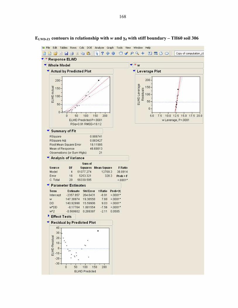
168

ELWD-Z1 contours in relationship with w and γγγγd with stiff boundary – TH60 soil 306

169

ELWD-Z1.5 contours in relationship with w and γγγγd with stiff boundary – TH60 soil 306

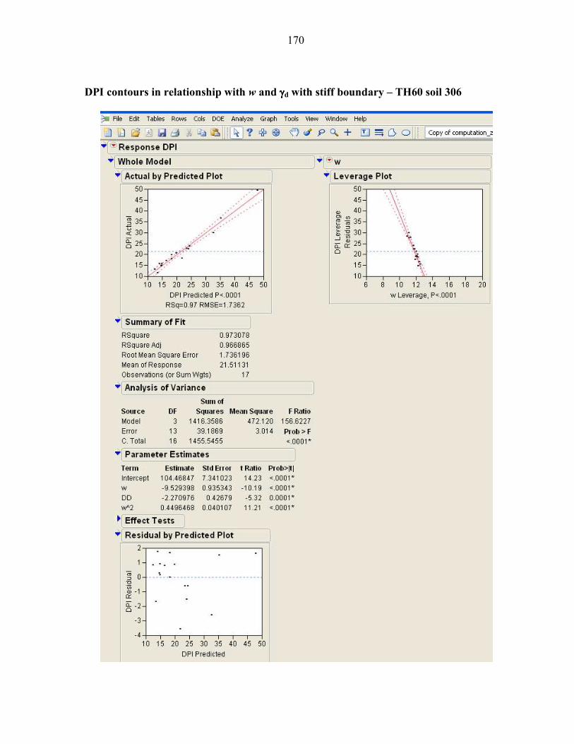
170

DPI contours in relationship with w and γγγγd with stiff boundary – TH60 soil 306

171

su contours in relationship with w and γγγγd with stiff boundary – TH60 soil 306

172

ττττG contours in relationship with w and γγγγd with stiff boundary – TH60 soil 306