Evacuation and Adaptation for Sea Level Rise

Evacuation and Adaptation for Sea Level Rise

Date:January22,2018

AphisitPhoowarawutthipanich,GraduateResearchAssistant,VirginiaTechPamelaMurray-Tuite,PhD,AssociateProfessor,ClemsonUniversityKathleenHancock,PhD,AssociateProfessor,VirginiaTechHeshamRakha,Ph.D.,P.Eng,Professor,VirginiaTechMohammadAljamal,GraduateStudent,VirginiaTechJianheDu,Ph.D.,SeniorResearchAssociate,VirginiaTechTransportationInstituteIhabEl-Shawarby,Ph.D.,VirginiaTechTransportationInstituteWillineRichardson,MorganStateUniversityBrianSmith,PhD,Professor,UniversityofVirginia

Preparedby:DepartmentofCivilEngineeringVirginiaTech7054HaycockRdFallsChurch,VA22043Preparedfor:VirginiaCenterforTransportationInnovationandResearch530EdgemontRoadCharlottesville,VA22903

FINAL REPORT

1. Report No.

2. Government Accession No. 3. Recipient’s Catalog No.

4. Title and Subtitle Evacuation and Adaptation for Sea Level Rise

5. Report Date October 10, 2017

6. Performing Organization Code

7. Author(s) Aphisit Phoowarawutthipanich, Pamela Murray-Tuite, Kathleen Hancock, Hesham Rakha, Mohammad Aljamal, Jianhe Du, Ihab El-Shawarby, Willine Richardson, Brian Smith

8. Performing Organization Report No.

9. Performing Organization Name and Address Department of Civil Engineering Virginia Tech 7054 Haycock Rd Falls Church, VA 22043

10. Work Unit No. (TRAIS

11. Contract or Grant No. DTRT13-G-UTC33

12. Sponsoring Agency Name and Address US Department of Transportation Office of the Secretary-Research UTC Program, RDT-30 1200 New Jersey Ave., SE Washington, DC 20590

13. Type of Report and Period Covered Final 5/10/16 – 8/30/17

14. Sponsoring Agency Code

15. Supplementary Notes

16. Abstract Sea level rise is becoming a major problem for transportation agencies.This study examines three issues: (1) identifying the impacts of sea level rise and storm surge on areas that may be evacuated from a hurricane, (2) evaluating microscopic and mesoscopic traffic simulation tools for evacuation scenarios, and (3) identifying adaptation strategies that could be useful for addressing sea level rise and protecting the road network. While hurricane evacuation notices are typically timed to attempt to clear evacuees from the roadways prior to the arrival of tropical storm force (or greater) winds, low lying areas must also be concerned about storm surge flooding, particularly for surge forerunners and as sea levels rise. This report uses water level time series data from the U.S. Army Corps of Engineers to identify the roads and areas of Norfolk and Virginia Beach vulnerable to storm surge flooding and sea level rise. The data were analyzed in conjunction with the terrain model. This study investigates three conditions, including (1) the base condition which is defined as the condition under storms modeled on mean sea level with wave effects, no sea level change, no astronomical tides, (2) the base condition plus tide, and (3) the base condition plus tide and 1.0 meter of sea level rise. For the analysis process, GIS was used to locate flooded areas and roads. Conditions 1 and 2 had similar results. The ranges of highest flood levels for conditions 2 and 3 are 1.5 to 4.5 meters and 2.5 to 5.2 meters, respectively. The percentages of flooded risk areas for condition 2 ranges from 4 % to 27%, while for condition 3 the range is 22% to 26% before the peak period, and more than half of the area is flooded during the peak period. This report compared the microscopic traffic simulation tool INTEGRATION and mesoscopic tool MATSim for modeling different evacuation scenarios. The models were compared based on the estimated evacuation time, average trip duration, and cumulative arrival plot. The estimated evacuation times of both INTEGRATION and MATSim were close to each other since the demand of all scenarios was less than the capacity of network. The evaluation showed a difference between the two models in the average trip duration. In INTEGRATION, the average trip duration increased with increasing traffic demand levels and decreasing roadway capacities. On the other hand, the average trip duration using MATSim decreased with increasing total travel time. The trends for the cumulative arrival times for both were close to each other. MATSim served more vehicles than INTEGRATION did at the

beginning of the stimulation. After that, both models served the same number of vehicles and these trends become closer to each other. These results seem to demonstrate that a tool like MATSim may produce erroneous conclusions if network-wide average results are desired. Geographic information systems (GIS) was used to study the topography and storm surge forecast of the Hampton Boulevard corridor of Norfolk Virginia. Potential adaptations were developed including Flood Barriers, Bio-retention Rain Garden Systems, and Flood walls to suit the area. Ultimately the finally decisions were made based on how feasible it was and cost effective on a long term bases.

17. Key Words Sea level rise; evacuation; traffic simulation; adaptation; storm surge; flood barriers; flood walls; bio-retention

18. Distribution Statement No restrictions. This document is available from the National Technical Information Service, Springfield, VA 22161

19. Security Classif. (of this report) Unclassified

20. Security Classif. (of this page) Unclassified

21. No. of Pages

22. Price

Acknowledgments

The authors thank the Hampton Roads Planning District Commission for providing data for this project.

Disclaimer

The contents of this report reflect the views of the authors, who are responsible for the facts and the accuracy of the information presented herein. This document is disseminated under the sponsorship of the U.S. Department of Transportation’s University Transportation Centers Program, in the interest of information exchange. The U.S. Government assumes no liability for the contents or use thereof.

TableofContents1 Introduction....................................................................................................................................1

1.1 Problem..................................................................................................................................................11.2 Organization of the Report................................................................................................................1

2 Evacuation Connectivity with Storm-Surge Flooding and Sea-Level Rise in Norfolk

and Virginia Beach.................................................................................................................................22.1 Research Questions..............................................................................................................................22.2 Study Area.............................................................................................................................................32.3 Literature Review.................................................................................................................................52.4 Data.........................................................................................................................................................8

2.4.1 Storm Surge Data...........................................................................................................................................82.4.2 Digital Elevation Data...............................................................................................................................11

2.5 Methodology........................................................................................................................................122.5.1 GIS Methodology for Flooding Analysis............................................................................................122.5.2 Generation of Time Period Scenarios...................................................................................................142.5.3 Connectivity Analysis................................................................................................................................16

2.6 Results...................................................................................................................................................162.7 Conclusions, Recommendations, and Future Research.............................................................24

3 Comparison of Microscopic and Mesoscopic Traffic Modeling Tools for Evacuation

Analysis..................................................................................................................................................263.1 Problem................................................................................................................................................263.2 Approach..............................................................................................................................................273.3 Methodology........................................................................................................................................27

3.3.1 INTEGRATION Simulation Model......................................................................................................273.3.2 MATSim Model...........................................................................................................................................28

3.4 Study Area...........................................................................................................................................293.4.1 Simulation File Construction and Calibration...................................................................................30

3.5 Findings................................................................................................................................................323.6 Conclusions and Recommendations...............................................................................................39

4 An Investigation of Climate Change Adaptation Case Study of the Hampton

Boulevard Corridor in Norfolk, Virginia.......................................................................................404.1 Literature Review...............................................................................................................................40

4.1.1 Background on Hampton Roads, Virginia..........................................................................................404.1.2 Background on Norfolk.............................................................................................................................414.1.3 Major Problems in Norfolk......................................................................................................................414.1.4 Fugro Atlantic Engineering Firm...........................................................................................................424.1.5 Adaptation Solutions Used Around the World..................................................................................42

4.2 Project Design.....................................................................................................................................444.2.1 Area of Focus................................................................................................................................................444.2.2 Methodology.................................................................................................................................................45

4.3 Solutions Analysis...............................................................................................................................474.3.1 Solution One - Flood Barrier One..........................................................................................................48

4.3.2 Solution Two – Flood Barrier Two.......................................................................................................484.3.3 Solution Three – Bio-retention Rain Garden System......................................................................494.3.4 Solution Four – Flood Walls...................................................................................................................49

4.4 Limitations and Conclusion/Recommendations..........................................................................494.4.1 Limitation.......................................................................................................................................................494.4.2 Conclusion.....................................................................................................................................................50

References.............................................................................................................................................51

List of Tables

Table1ClassificationSchemeforFloodingConditions........................................................................14Table2ResultsofGIS-basedFloodingAnalysisforAllScenarios....................................................19Table3LengthofFloodedRoadsinMilesforAllScenarios...............................................................23Table4FundamentalInputDataFiles(VanAerdeandRakha2007)...........................................28Table5Definitionsofthe11Scenarios......................................................................................................30Table6EstimatedEvacuationTimeofthe11ScenariosinBothModels....................................33Table7AverageTripDurationforthe11Scenarios.............................................................................34Table8MeasureofEffectivenessforthe11Scenarios.........................................................................39

List of Figures

Figure1LocationofNorfolkandVirginiaBeach,Virginia.....................................................................4Figure2MasterTracksPassingNorfolkandVirginiaBeach..............................................................10Figure3WorkflowProcessoftheStormSurgeTimeSeriesDatabase..........................................11Figure4GIS-basedFloodingAnalysisProcessforEachTimeStep.................................................13Figure5ModeledTime-SeriesofWater-SurfaceElevationforSavePoint(16869)................14Figure6PotentialTimeStepsforModelingTime-SeriesWater-SurfaceElevations...............15Figure7StormSurgeFloodingSimulationofStorm22inNorfolkandVirginiaBeach,

Virginia.............................................................................................................................................................18Figure8IsolatedNetworksExposedtoStormSurgeandSeaLevelRise,Norfolkand

VirginiaBeach,Virginia.............................................................................................................................22Figure9NumberofIsolatedNetworksforAllScenarios.....................................................................22Figure10ComparisonofLengthofFloodedRoads................................................................................23Figure11StagesofaMATSimsimulation(MarcelRieserandGregorL�ammel2014).......29Figure12Knoxville,TN(Source:GoogleMaps)......................................................................................29Figure13CountstationsandroadwaynetworkinKnoxville,TN,area.......................................31Figure14Relationshipbetweenobservedlinkvolumevs.simulationvolume........................32Figure15ScreenshotofINTEGRATIONsoftwareinterfaceforScenario10..............................33Figure16Estimatedevacuationtimeofthe11scenariosforbothmodels................................34Figure17Averagetripdurationforthe11scenarios..........................................................................34Figure18Summerseasonscenarios(a)normalweathermidweekdaytime(b)adverse

weathermidweekdaytime(c)normalweatherweekenddaytime(d)normalweathermidweekandweekendeveningperiod.............................................................................................36

Figure19Winterseasonscenarios(a)normalweathermidweekdaytime(b)adverseweathermidweekdaytime(c)normalweatherweekenddaytime(d)normalweathermidweekandweekendeveningperiod.............................................................................................37

Figure20Differentscenarios(a)roadwayimpact(b)peakconstruction(c)futurepurposes..........................................................................................................................................................38

Figure21HighTideFloodingalongHamptonBoulevard..................................................................45Figure22ElevationAlongHamptonBoulevard,Norfolk....................................................................46Figure23PossibleSolutionsfortheHamptonBoulevardArea.......................................................47Figure24FloodBarrierOneDesignfortheHamptonBoulevardAreaandInspiration.......48Figure25ExampleofBio-retentionBasin/RainGardenDesignfortheHampton

BoulevardArea.............................................................................................................................................49

1

1 Introduction Global sea level rise results from an increase in the volume and quantity (or mass) of water in the world’s oceans. The major cause of the increased water volume is rising atmospheric and ocean temperatures, due to thermal expansion (Titus and Anderson 2009). Sea level rise caused by an increase in volume is referred to as steric sea level rise. The melting of more ice sheets, glaciers, and snow attributed to rising atmospheric temperatures adds water (volume and mass) to the world’s oceans. In addition to rising temperature, ocean currents, and winds, the vertical movement of land can have a significant effect at the local level. There are two types of vertical land movement: uplift (land rising) and subsidence (land sinking). Subsidence, which is considered a significant factor in the rate of sea level rise in the Hampton Roads (Titus and Anderson 2009), or Tidewater, region (which includes Virginia Beach and Norfolk), occurs due to the sediment compaction or extraction of subsurface liquids, such as water or oil. Scientists from the Virginia Institute of Marine Science have estimated that subsidence accounts for approximately one-half to two-thirds of the sea level rise experienced in the Hampton Roads region (Boon, Brubaker et al. 2010). Sea level rise poses issues to coastal areas for both normal and evacuation traffic operations. During hurricanes, sea level rise and storm surge can flood low lying areas, including roadways that may be used for evacuation. Depending on the time the storm surge arises, some evacuees may be trapped by flood waters. 1.1 Problem This study examines three issues. The first identifies the impacts of sea level rise and storm surge on areas that may be evacuated from a hurricane. The impacts include the percentage of flooded area and areas that become disconnected from the rest of the road network. These areas may need to be evacuated for water hazards, depending on the depth of the flood, as well as for wind hazards from hurricanes. The second issue is the selection of the appropriate traffic simulation tool for evacuation traffic. Microscopic and mesoscopic tools are compared. The third issue involves identifying adaptation strategies that could be useful for addressing sea level rise and protecting the road network. 1.2 Organization of the Report This report has three major chapters. Each chapter has its own approach, results, conclusions, and recommendations. Chapter 2 describes a study of road network connectivity under hurricane storm surge and sea level rise conditions and was authored by Aphisit Phoowarawutthipanich, Dr. Pam Murray-Tuite, and Dr. Kathleen Hancock. Chapter 3 compares microscopic and mesoscopic traffic simulation tools for evacuation modeling and was authored by Dr. Hesham Rakha, Mohammad Aljamal, Dr. Jianhe Du, and Dr. Ihab El-Shawarby. Finally, Chapter 4 presents potential adaptation strategies for sea level rise and was authored by Willine Richardson and Dr. Brian Smith.

2

2 Evacuation Connectivity with Storm-Surge Flooding and Sea-Level Rise in Norfolk and Virginia Beach

While evacuation notices are typically timed to attempt to clear evacuees from the roadways prior to the arrival of tropical storm force (or greater) winds, low lying areas must also be concerned about storm surge flooding, particularly for surge forerunners and as sea levels rise. Coastal flooding can result from storm surge, sea-level rise, and shoreline change. Location is a major factor in the flooding event; a low-lying area with a low-gradient is likely to be flooded. Therefore, there are high probabilities that vulnerable areas situated along the coast will be inundated when hurricane storm surges arrive. The expansion of the area covered by hurricane storm surges in coastal areas is increasingly caused by sea-level rise. The trend of sea level rise at the Sewell’s Point monitoring station near the Virginia Beach areas shows that the sea level increased 4.44 millimeter per year from 1927 to 2006, and this will increase to 1.46 feet over 100 years (National Oceanic and Atmospheric Administration 2011). This rise will exacerbate storm surge in this area whether that surge arrives prior to the hurricane or at the same time. Hurricane Ike is a well-known example of a surge forerunner that affected the ability of evacuees to reach safety. Hurricane Ike, one of 16 tropical storms in 2008, has been regarded as one of the most powerful storm to hit the Texas coast line since 1915 because of its high storm surge. The peak storm surge height was approximately 15-20 feet at Bolivar Peninsula, TX. Damage estimates were $29.5 billion, making Hurricane Ike the second costliest hurricane to hit the U.S. This storm caused 103 deaths with 23 missing people (TropicalWeather.net no date). While Hurricane Ike made landfall on September 13 at 2:10 am CDT at Galveston, TX, parts of the Texas and southwest Louisiana coast were flooded 24 hours earlier. Even though a 10-15 foot tall tide is generally seen in these areas, a storm surge of 13 feet and higher was observed in Galveston. For a variety of reasons (e.g., storm changing directions, prior experience from Hurricane Rita), mandatory evacuation orders for the Galveston area were delayed, issued on the evening of September 11 (Rice 2016). This timing left only a little over one day to evacuate before the hurricane made landfall and when the early storm surge was causing flooding. Storm surge forerunners could occur in other areas as well, affecting evacuation capabilities. This study examines the impact of storm surge and sea level rise on road connectivity for the Virginia Beach and Norfolk area under three conditions for a synthetic tropical storm: (1) storm surge only (base conditions), (2) base conditions and tide, and (3) base conditions, tide, and 1.0 m of sea level rise. These conditions were evaluated for five time periods (called scenarios), starting 12 hours before the peak surge height. 2.1 Research Questions This chapter investigates two research questions related to the road network vulnerability to storm surge and sea level rise.

3

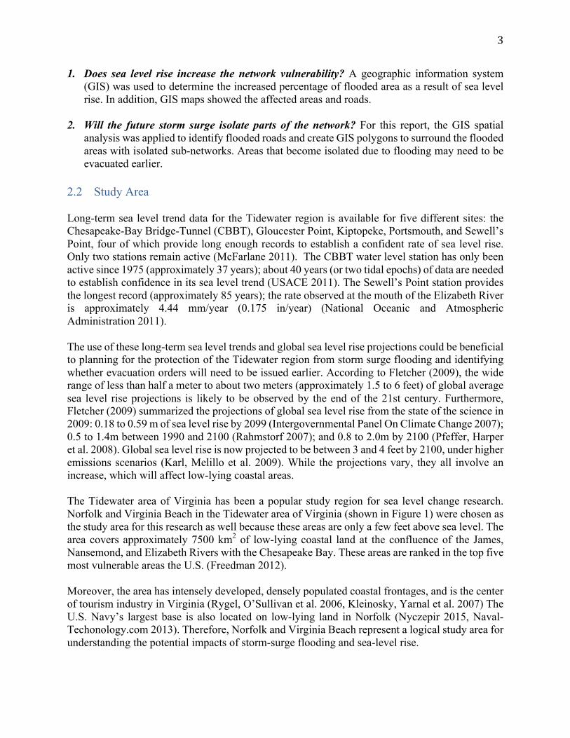
1. Does sea level rise increase the network vulnerability? A geographic information system (GIS) was used to determine the increased percentage of flooded area as a result of sea level rise. In addition, GIS maps showed the affected areas and roads.

2. Will the future storm surge isolate parts of the network? For this report, the GIS spatial

analysis was applied to identify flooded roads and create GIS polygons to surround the flooded areas with isolated sub-networks. Areas that become isolated due to flooding may need to be evacuated earlier.

2.2 Study Area Long-term sea level trend data for the Tidewater region is available for five different sites: the Chesapeake-Bay Bridge-Tunnel (CBBT), Gloucester Point, Kiptopeke, Portsmouth, and Sewell’s Point, four of which provide long enough records to establish a confident rate of sea level rise. Only two stations remain active (McFarlane 2011). The CBBT water level station has only been active since 1975 (approximately 37 years); about 40 years (or two tidal epochs) of data are needed to establish confidence in its sea level trend (USACE 2011). The Sewell’s Point station provides the longest record (approximately 85 years); the rate observed at the mouth of the Elizabeth River is approximately 4.44 mm/year (0.175 in/year) (National Oceanic and Atmospheric Administration 2011). The use of these long-term sea level trends and global sea level rise projections could be beneficial to planning for the protection of the Tidewater region from storm surge flooding and identifying whether evacuation orders will need to be issued earlier. According to Fletcher (2009), the wide range of less than half a meter to about two meters (approximately 1.5 to 6 feet) of global average sea level rise projections is likely to be observed by the end of the 21st century. Furthermore, Fletcher (2009) summarized the projections of global sea level rise from the state of the science in 2009: 0.18 to 0.59 m of sea level rise by 2099 (Intergovernmental Panel On Climate Change 2007); 0.5 to 1.4m between 1990 and 2100 (Rahmstorf 2007); and 0.8 to 2.0m by 2100 (Pfeffer, Harper et al. 2008). Global sea level rise is now projected to be between 3 and 4 feet by 2100, under higher emissions scenarios (Karl, Melillo et al. 2009). While the projections vary, they all involve an increase, which will affect low-lying coastal areas. The Tidewater area of Virginia has been a popular study region for sea level change research. Norfolk and Virginia Beach in the Tidewater area of Virginia (shown in Figure 1) were chosen as the study area for this research as well because these areas are only a few feet above sea level. The area covers approximately 7500 km2 of low-lying coastal land at the confluence of the James, Nansemond, and Elizabeth Rivers with the Chesapeake Bay. These areas are ranked in the top five most vulnerable areas the U.S. (Freedman 2012). Moreover, the area has intensely developed, densely populated coastal frontages, and is the center of tourism industry in Virginia (Rygel, O’Sullivan et al. 2006, Kleinosky, Yarnal et al. 2007) The U.S. Navy’s largest base is also located on low-lying land in Norfolk (Nyczepir 2015, Naval-Techonology.com 2013). Therefore, Norfolk and Virginia Beach represent a logical study area for understanding the potential impacts of storm-surge flooding and sea-level rise.

4

Figure1LocationofNorfolkandVirginiaBeach,Virginia

5

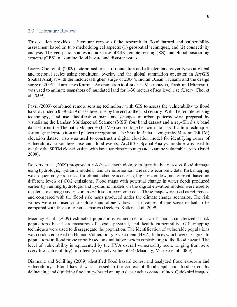
2.3 Literature Review This section provides a literature review of the research in flood hazard and vulnerability assessment based on two methodological aspects: (1) geospatial techniques, and (2) connectivity analysis. The geospatial studies included use of GIS, remote sensing (RS), and global positioning systems (GPS) to examine flood hazard and disaster issues. Usery, Choi et al. (2009) determined areas of inundation and affected land cover types at global and regional scales using conditional overlay and the global summation operation in ArcGIS Spatial Analyst with the historical highest surge of 2004’s Indian Ocean Tsunami and the design surge of 2005’s Hurricanes Katrina. An animation tool, such as Macromedia, Flash, and Microsoft, was used to animate snapshots of inundated land for 1-30 meters of sea level rise (Usery, Choi et al. 2009). Pavri (2009) combined remote sensing technology with GIS to assess the vulnerability to flood hazards under a 0.38−0.59 m sea level rise by the end of the 21st century. With the remote sensing technology, land use classification maps and changes in urban patterns were prepared by visualizing the Landsat Multispectral Scanner (MSS) four band dataset and a gap-filled six band dataset from the Thematic Mapper + (ETM+) sensor together with the classification techniques for image interpretation and pattern recognition. The Shuttle Radar Topography Mission (SRTM) elevation dataset also was used to construct a digital elevation model for identifying zones of vulnerability to sea level rise and flood events. ArcGIS’s Spatial Analyst module was used to overlay the SRTM elevation data with land use classes to map and examine vulnerable areas (Pavri 2009). Deckers et al. (2009) proposed a risk-based methodology to quantitatively assess flood damage using hydrologic, hydraulic models, land use information, and socio-economic data. Risk mapping was sequentially processed for climate change scenarios; high, mean, low, and current, based on different levels of CO2 emissions. Flood maps with potential change in water depth produced earlier by running hydrologic and hydraulic models on the digital elevation models were used to recalculate damage and risk maps with socio-economic data. These maps were used as references and compared with the flood risk maps produced under the climate change scenarios. The risk values were not used as absolute stand-alone values - risk values of one scenario had to be compared with those of other scenarios (Deckers, Kellens et al. 2009). Maantay et al. (2009) estimated populations vulnerable to hazards, and characterized at-risk populations based on measures of social, physical, and health vulnerability. GIS mapping techniques were used to disaggregate the population. The identification of vulnerable populations was conducted based on Human Vulnerability Assessment (HVA) Indices which were assigned to populations in flood prone areas based on qualitative factors contributing to the flood hazard. The level of vulnerability is represented by the HVA overall vulnerability score ranging from zero (very low vulnerability) to fifteen (extremely vulnerable) (Maantay, Maroko et al. 2009). Bizimana and Schilling (2009) identified flood hazard zones, and analyzed flood exposure and vulnerability. Flood hazard was assessed in the context of flood depth and flood extent by delineating and digitizing flood maps based on input data, such as contour lines, Quickbird images,

6

Digital Elevation Models (DEM), and flood depth information from household surveys which was estimated based on watermarks found on the houses with reference to the ground. The authors performed a flood exposure analysis for elements at risk: vulnerable infrastructure (roads, bridges, water supply), buildings, population and economic activities. Afterwards, exposed elements were overlaid on the flood zones (Bizimana and Schilling 2009). McFarlane (2012) used GIS to identify vulnerable areas that could be inundated by storm surge and sea level rise under the one meter of sea level rise above Spring high tide scenario. Population, property, and number of employees were included in the analysis. Using tidal conditions to reference the elevation dataset, was not part of McFarlane’s previous (McFarlane 2011) work. Moreover, McFarlane (2012) focused specifically on sea level rise; whereas, storm surge zones resulting from the elevation model and storm surge model were used in his previous study (McFarlane 2011) to produce storm surge flooding maps. Failure to consider the benchmark of the elevation dataset made McFarlane’s (2011) earlier work less reliable than his later work. Kleinosky et al. (2007) assessed the road network vulnerability to sea level rise and storm-surge flooding in Hampton Roads, Virginia for all five categories of hurricane based on the assumption that the expansion of the flooded areas caused by the storm surges could result from sea level rise. The storm heights were added to the sea level rise of 20 cm projected for a 100 year period. This was useful for developing scenarios with storm surges and sea level rise as uncertainty in storm height is difficult to predict by any model. Unlike McFarlane (2011), it used the storm surge zones taken from previous studies without adjusting the storm surge heights. In addition to the present day flooding scenario, future impacts of sea level rise on the flooding events were illustrated with the projected population, distribution and planned development of land use. Scenarios were also developed that address uncertainties regarding future population growth and distribution (Kleinosky, Yarnal et al. 2007). All earlier studies have similarity in some aspects. They used GIS as a major tool for identifying the flood extent areas although remote processing technologies and GPS were incorporated in the methodology to prepare the flood maps in some research works (Bizimana and Schilling 2009, Pavri 2009). The data preparation of Maantay et al. (2009) was conducted using ArcGIS to disaggregate population data (e.g., from the census) into much higher resolution data, giving a more realistic depiction of population locations and densities (Maantay, Maroko et al. 2009), and the approach proposed by Pavri (2009) is another example of transforming data before further analysis. The previous literature indicated that geomatics were useful to vulnerability assessment for dealing with spatial datasets attributed to the hazard and disaster. Moreover, overlay analysis was frequently utilized for various purposes. In addition, an interesting aspect that all the previous research works shared was the use of the predicted sea level rise as a secondary dataset for the analysis rather than modeling the sea level rise data for this issue. Similarly, this study utilized the sea level rise levels which were previously projected by other models for the flood analysis. However, the dissimilarity in these studies can be described as follows. Almost all previous works determined water depths including the effects of sea level rise and storm surge for the vulnerability assessment in different ways. Usery et al. (2009) made use of the historical surge data for

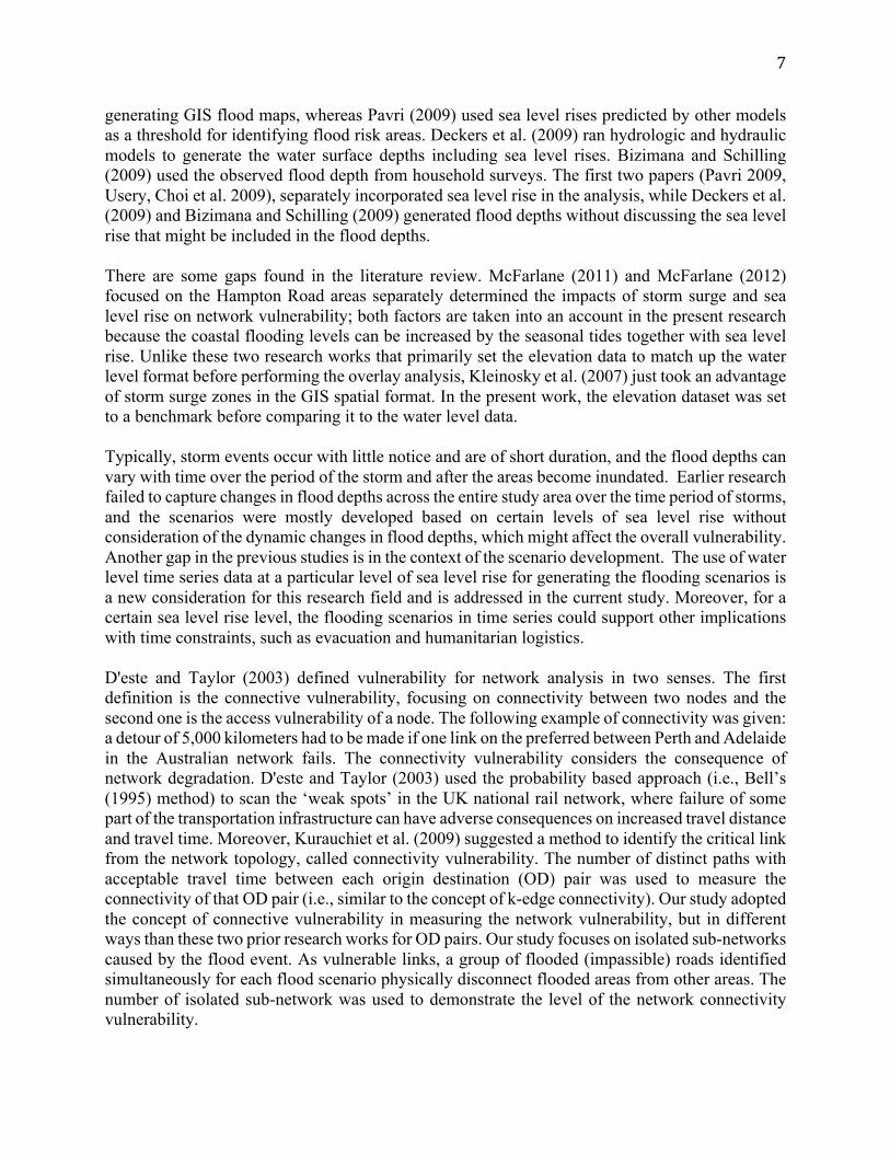
7

generating GIS flood maps, whereas Pavri (2009) used sea level rises predicted by other models as a threshold for identifying flood risk areas. Deckers et al. (2009) ran hydrologic and hydraulic models to generate the water surface depths including sea level rises. Bizimana and Schilling (2009) used the observed flood depth from household surveys. The first two papers (Pavri 2009, Usery, Choi et al. 2009), separately incorporated sea level rise in the analysis, while Deckers et al. (2009) and Bizimana and Schilling (2009) generated flood depths without discussing the sea level rise that might be included in the flood depths. There are some gaps found in the literature review. McFarlane (2011) and McFarlane (2012) focused on the Hampton Road areas separately determined the impacts of storm surge and sea level rise on network vulnerability; both factors are taken into an account in the present research because the coastal flooding levels can be increased by the seasonal tides together with sea level rise. Unlike these two research works that primarily set the elevation data to match up the water level format before performing the overlay analysis, Kleinosky et al. (2007) just took an advantage of storm surge zones in the GIS spatial format. In the present work, the elevation dataset was set to a benchmark before comparing it to the water level data. Typically, storm events occur with little notice and are of short duration, and the flood depths can vary with time over the period of the storm and after the areas become inundated. Earlier research failed to capture changes in flood depths across the entire study area over the time period of storms, and the scenarios were mostly developed based on certain levels of sea level rise without consideration of the dynamic changes in flood depths, which might affect the overall vulnerability. Another gap in the previous studies is in the context of the scenario development. The use of water level time series data at a particular level of sea level rise for generating the flooding scenarios is a new consideration for this research field and is addressed in the current study. Moreover, for a certain sea level rise level, the flooding scenarios in time series could support other implications with time constraints, such as evacuation and humanitarian logistics. D'este and Taylor (2003) defined vulnerability for network analysis in two senses. The first definition is the connective vulnerability, focusing on connectivity between two nodes and the second one is the access vulnerability of a node. The following example of connectivity was given: a detour of 5,000 kilometers had to be made if one link on the preferred between Perth and Adelaide in the Australian network fails. The connectivity vulnerability considers the consequence of network degradation. D'este and Taylor (2003) used the probability based approach (i.e., Bell’s (1995) method) to scan the ‘weak spots’ in the UK national rail network, where failure of some part of the transportation infrastructure can have adverse consequences on increased travel distance and travel time. Moreover, Kurauchiet et al. (2009) suggested a method to identify the critical link from the network topology, called connectivity vulnerability. The number of distinct paths with acceptable travel time between each origin destination (OD) pair was used to measure the connectivity of that OD pair (i.e., similar to the concept of k-edge connectivity). Our study adopted the concept of connective vulnerability in measuring the network vulnerability, but in different ways than these two prior research works for OD pairs. Our study focuses on isolated sub-networks caused by the flood event. As vulnerable links, a group of flooded (impassible) roads identified simultaneously for each flood scenario physically disconnect flooded areas from other areas. The number of isolated sub-network was used to demonstrate the level of the network connectivity vulnerability.

8

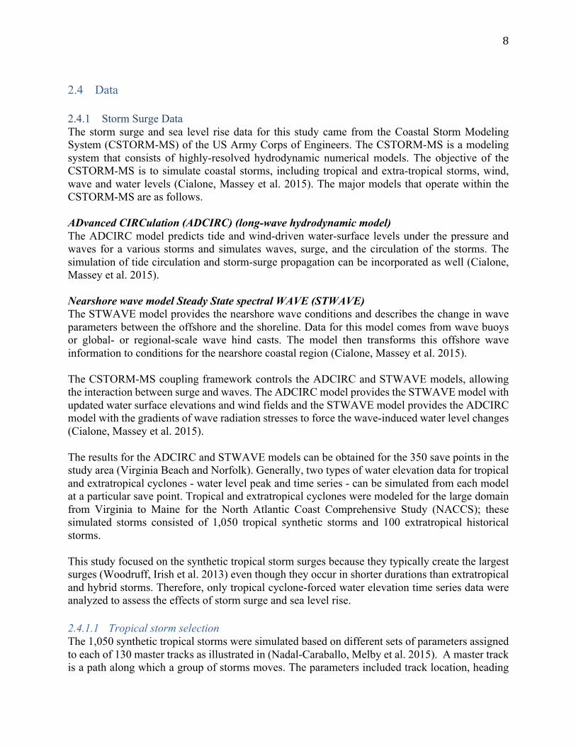
2.4 Data 2.4.1 Storm Surge Data The storm surge and sea level rise data for this study came from the Coastal Storm Modeling System (CSTORM-MS) of the US Army Corps of Engineers. The CSTORM-MS is a modeling system that consists of highly-resolved hydrodynamic numerical models. The objective of the CSTORM-MS is to simulate coastal storms, including tropical and extra-tropical storms, wind, wave and water levels (Cialone, Massey et al. 2015). The major models that operate within the CSTORM-MS are as follows. ADvanced CIRCulation (ADCIRC) (long-wave hydrodynamic model) The ADCIRC model predicts tide and wind-driven water-surface levels under the pressure and waves for a various storms and simulates waves, surge, and the circulation of the storms. The simulation of tide circulation and storm-surge propagation can be incorporated as well (Cialone, Massey et al. 2015). Nearshore wave model Steady State spectral WAVE (STWAVE) The STWAVE model provides the nearshore wave conditions and describes the change in wave parameters between the offshore and the shoreline. Data for this model comes from wave buoys or global- or regional-scale wave hind casts. The model then transforms this offshore wave information to conditions for the nearshore coastal region (Cialone, Massey et al. 2015). The CSTORM-MS coupling framework controls the ADCIRC and STWAVE models, allowing the interaction between surge and waves. The ADCIRC model provides the STWAVE model with updated water surface elevations and wind fields and the STWAVE model provides the ADCIRC model with the gradients of wave radiation stresses to force the wave-induced water level changes (Cialone, Massey et al. 2015). The results for the ADCIRC and STWAVE models can be obtained for the 350 save points in the study area (Virginia Beach and Norfolk). Generally, two types of water elevation data for tropical and extratropical cyclones - water level peak and time series - can be simulated from each model at a particular save point. Tropical and extratropical cyclones were modeled for the large domain from Virginia to Maine for the North Atlantic Coast Comprehensive Study (NACCS); these simulated storms consisted of 1,050 tropical synthetic storms and 100 extratropical historical storms. This study focused on the synthetic tropical storm surges because they typically create the largest surges (Woodruff, Irish et al. 2013) even though they occur in shorter durations than extratropical and hybrid storms. Therefore, only tropical cyclone-forced water elevation time series data were analyzed to assess the effects of storm surge and sea level rise. 2.4.1.1 Tropical storm selection The 1,050 synthetic tropical storms were simulated based on different sets of parameters assigned to each of 130 master tracks as illustrated in (Nadal-Caraballo, Melby et al. 2015). A master track is a path along which a group of storms moves. The parameters included track location, heading

9

direction, central pressure deficit, radius of maximum wind, and translational speed. Each of the 1,050 tropical synthetic storms was simulated in time series under three conditions. The first condition represents the base condition in which the simulation of storm surges was performed on mean sea level with wave effects, but no tides or long term sea level change were included. The second condition extended the base condition by including wave effects and a unique randomly-selected tide phase but no sea level change. The third condition was developed further from the second by including one meter of global sea level rise (GSLR) in the hydrodynamic simulations under the assumption that a simple addition of 1 meter sea level rise can be simulated with the storm surges to reasonably approximate water heights. A boundary was created for the study area using the GIS tool. A new polygon feature was created in a shape file as a boundary, and this boundary layer helped identify the save points within the study area. The boundary also highlighted the study area affected by the flooding event in order to prepare the DEM within the boundary. On average, a master track included eight synthetic tropical storms. Accordingly, only 72 synthetic storms were carried by nine master tracks passing by the study area resulting from the boundary creation (Virginia Beach and Norfolk) and shown in Figure 2. This study selected 1 out of 72 tropical storms for demonstrating the effect of sea level rise on storm surge flooding. From this set of 72 storms, the most influential storm, defined as the storm that affected the highest number of save points in the area, was selected. Save points impacted by a storm were based on the centerline of the storm (the storm eye); GIS buffer analysis was performed to create buffers from the storm tracks to determine how many save points would be affected by each storm. With certain buffer distances, the storm that covered the most points became the worst storm for this study. Staring at the 1 km buffer for all storms, the buffer distances were gradually increased to cover as many save points as possible. After the buffer distances of all the storms reached 20 km from the centerlines, tropical storm ID 22 became the first storm to include all of the save points in its buffer and was selected for this study. The 20 km threshold was within the NACCS spacing limit of 60 km (Nadal-Caraballo, Melby et al. 2015).

10

Source:Generatedbyusingthecoastalhazardsysteminterfacemapavailableathttps://chs.erdc.dren.mil/

Figure2MasterTracksPassingNorfolkandVirginiaBeach

2.4.1.2 Data Preparation At each save point, water elevation time series data of 1,050 simulated tropical storms were generated in one file. The water elevations were measured every 10 minutes for 4 to 7 days depending on the simulated tropical storm. Consequently, one time series data file contained thousands of water elevation values for a single save point. With 350 save points of interest, millions of water elevation records had to be processed. Only storm ID 22 had to be pulled for each of the three conditions. Therefore, the data processing steps were carefully designed as illustrated in Figure 3.

11

Figure3WorkflowProcessoftheStormSurgeTimeSeriesDatabase

The SQL database was used to produce three data files per time step for all three conditions, each of which contained water levels of all save points across the study area for a time step of the flooding event. The SQL database pulled the water elevations of the selected tropical storm (ID 22) for a specified time interval for all the save points. The water height dataset of the 10 minute snapshot for the entire area prepared by the previous step was generated in MS Excel format. This file was then transformed to a GIS water height layer at the save points. The water height layers produced by the GIS tools were investigated in two aspects for the data cleaning process. First, all false zero meter water heights were removed from the water height layers because those erroneous data can deviate the raster water surface which will be interpolated from water heights at save points across the area. 2.4.2 Digital Elevation Data In addition to the storm information, data on the study area’s land elevation was obtained from the Hampton Roads Planning District Commission. This data consisted of a 5-foot resolution Digital Elevation Model (DEM) benchmarked to the North American Vertical Datum of 1988 (NAVD 88) with the vertical unit in feet and developed using the most recent LiDAR-derived elevation data. The DEM is considered a key part of any study of vulnerability to storm surge flooding and sea level rise. This dataset was considered consistent for the entire region with a readily understandable vertical reference point. This dataset included relative imprecision (5-foot pixels) and uncertainty, which decreased its utility when addressing increments of sea level rise less than approximately three feet. While this dataset should not be used for delineating areas for legal purposes, it can be useful for identifying areas for further, more detailed study as well as for general impacts over large geographic areas (though not for projecting future shorelines (McFarlane 2012)).

Request

Condition Storm ID

Scenario (10 minute time interval)

Input

Water height time series data files for all save points

Output

A data file containing water heights for the entire study area

in a snapshot

SQL Database

Extract one record of water height data by the request from

each data file Arrange all the water height

records

12

2.5 Methodology The methodology had three major components. The first component generated the water height data and produced the water height layer as outlined in Figure 4 and addresses research question 1. The second component consisted of a GIS-based process to determine the flooded areas and roads as well as flood heights. The third component demonstrated the analysis time points which were selected from the water height time series data, and the first two components were used to calculate flooding of roadways at each of the time periods for each of the three scenarios. Comparing the flooding at the different time periods across the scenarios helped address the second research question. Finally, the flooded roadways at the different time periods were used in conjunction with connectivity analysis to identify disconnected networks (research question 2). 2.5.1 GIS Methodology for Flooding Analysis This part of the methodology was designed for two purposes. First, the flooded areas and roads were identified. Second, the GIS-based method determined how much they would be inundated by storm surge flooding and sea level rise. Details of the methodology are described below.

1. Generation of raster water surfaces for each of the three conditions: The inverse distance weighted technique (IDW) was used to interpolate a raster surface from water heights earlier generated as point features from the water heights dataset for all the save points across the study area. At the end of this step, all the water heights treated as point features were transformed to the raster format.

2. Calculation of flooded areas: The elevation values of the terrain model (DEM) were subtracted from the water heights from the water surface across the study area, and then the flood surface was classified into ranges to show the difference between flooded areas and unflooded areas. Ranges of flood heights shown in different colors of polygons could be used for illustrating flooding levels. The ranges are specified and interpreted in Table 1.

3. Identification of flooded roads: A spatial join was used to compare road elevations to water levels measured from the ground. This tool joined attributes from one feature to another based on the spatial relationship. The target features and the joined attributes from the join features were written to the output feature class.

13

Figure4GIS-basedFloodingAnalysisProcessforEachTimeStep

GIS Data Processing

Create Water Height Layer Output: Water level layer showing water heights at all the save points (point layer)

Obtain Water Height (At each save point, water levels measured in meters)

Clean Water Height Layer - Remove all water heights with no data records Output: water height layer ready for IDW

Create Study Area Layer and Prepare DEM within the boundary

(Study Areas: Norfolk and Virginia Beach)

Generate Water Surface Bring water heights (point layer) in DEM and use IDW to predict water surface

Output: Water Surface in Raster

Identify flooded Areas and determine how much they are flooded Bring flooded polygon layers and terrain model

Water Level Layer - (minus) DEM Output: Flooded areas highlighted

Find flooded roads Compare road elevations to water level using Spatial Join

Output: Flooded roads highlighted

14

Table1ClassificationSchemeforFloodingConditions

Range of Flood (m) Flooding Conditions

Lowest - -5.00 Unflooded -5.00 - -0.05 Unflooded -0.05 - 0.05 Unflooded 0.05 - 0.50 Flooded 0.50 - 1.00 Flooded 1.00 - 2.00 Flooded 2.00 - 3.00 Flooded 3.00 - 4.00 Flooded

4..00+ Flooded 2.5.2 Generation of Time Period Scenarios Five-day water level time series of tropical storm ID 22 for all the save points were separately collected for three different conditions and the water levels over the five days varied by the save point locations. The time interval for this study was specified as the time period from when the study area started to be inundated to the time when it reached the peak.

To identify interesting time periods for the flooding analysis, GIS visualization and graphs were used. The GIS visualizations indicated the spatial water levels throughout the study area while graphs, such as that in Figure 5, were helpful to visualize water levels over the five day time horizon. The process of selecting the interesting time intervals for this research can be described as follows.

Figure5ModeledTime-SeriesofWater-SurfaceElevationforSavePoint(16869)

-1

0

1

2

3

4

5

1 14 27 40 53 66 79 92 105

118

131

144

157

170

183

196

209

222

235

248

261

274

287

300

313

326

339

352

365

378

391

404

417

430

443

456

WaterLe

vel(meters)

Time(10minuteinterval)

TimeSeriesWaterElevationsforPoint16869

Condition1(Surge) Condition2(Surge+Tide) Condition3(Surge+Tide+SeaLevelRise)

15

First, the five-day water level time series of tropical storm ID 22 for three conditions were graphed together to observe the characteristics of water levels for all the save points, generating a total of 350 water level time series plots. Most of the water level time series plots had similar trends to those shown in Figure 5, but their peaks were sometimes observed at different times within the three hour period over the peak in Figure 5. Therefore, a representative peak (simulation time 352 – shown in Figure 6) was chosen and treated as the end time of the study period for the analysis.

Figure6PotentialTimeStepsforModelingTime-SeriesWater-SurfaceElevations

Second, the start time of the study period was identified with the application of GIS maps. The same set of snapshots that would be shared by all the three conditions were developed. The water level time series data over the simulation length of storm Id 22 for some representative save points were examined with graphs for all three conditions. The process was started with condition 3 which is considered the worst storm surge condition with the effect of sea level rise. As illustrated in Figure 6, a potential set of time steps leading up to the peak of condition 3 was initially chosen as primary time steps for the scenario generation. These time steps were expected to show the significant changes in flooded areas for the study area. The GIS flooding maps were generated for all the primary time steps, and the changes in flooded areas were then investigated to select the candidate set of time steps. The candidate set of time steps with different sizes of flooded areas was tested later on by the water level time series data set of condition 2 to check whether or not the same patterns of flooded areas would be seen for these candidate time steps. Moreover, this step could reduce the number of time steps to be selected as scenarios after generating the flooding maps with the data set of condition 2. As seen in Figure 6, condition 1 and 2 have the same trend of water level time series, but with the water heights are fluctuated by tide in condition 2. Including tides was more realistic and the results displayed below are for conditions 2 and 3 because the timing for condition 2 is equivalent to condition 1 over the entire period. The selected time steps from condition 2 helped verify the candidates from 3, and the final time steps were generated for the mapping process. For the smaller set of time steps, the GIS flooding maps provided time steps

-1

0

1

2

3

4

5

1 14 27 40 53 66 79 92 105

118

131

144

157

170

183

196

209

222

235

248

261

274

287

300

313

326

339

352

365

378

391

404

417

430

443

456

WaterLe

vel(meters)

Time(10minuteinterval)

TimeSeriesWaterElevationsforPoint17018

Condition1(Surge) Condition2(Surge+Tide) Condition3(Surge+Tide+SeaLevelRise)

PotentialTimeStep

TimeStep250 TimeStep352

16

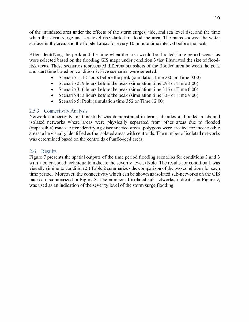
of the inundated area under the effects of the storm surges, tide, and sea level rise, and the time when the storm surge and sea level rise started to flood the area. The maps showed the water surface in the area, and the flooded areas for every 10 minute time interval before the peak. After identifying the peak and the time when the area would be flooded, time period scenarios were selected based on the flooding GIS maps under condition 3 that illustrated the size of flood-risk areas. These scenarios represented different snapshots of the flooded area between the peak and start time based on condition 3. Five scenarios were selected:

• Scenario 1: 12 hours before the peak (simulation time 280 or Time 0:00) • Scenario 2: 9 hours before the peak (simulation time 298 or Time 3:00) • Scenario 3: 6 hours before the peak (simulation time 316 or Time 6:00) • Scenario 4: 3 hours before the peak (simulation time 334 or Time 9:00) • Scenario 5: Peak (simulation time 352 or Time 12:00)

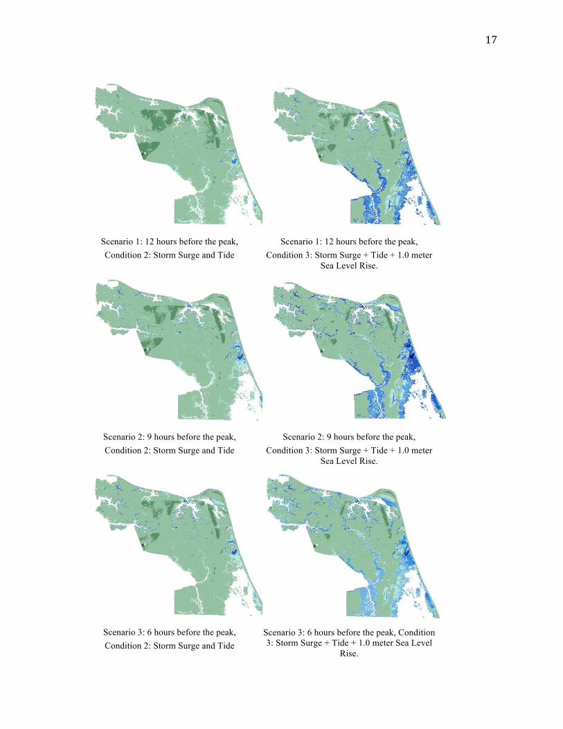
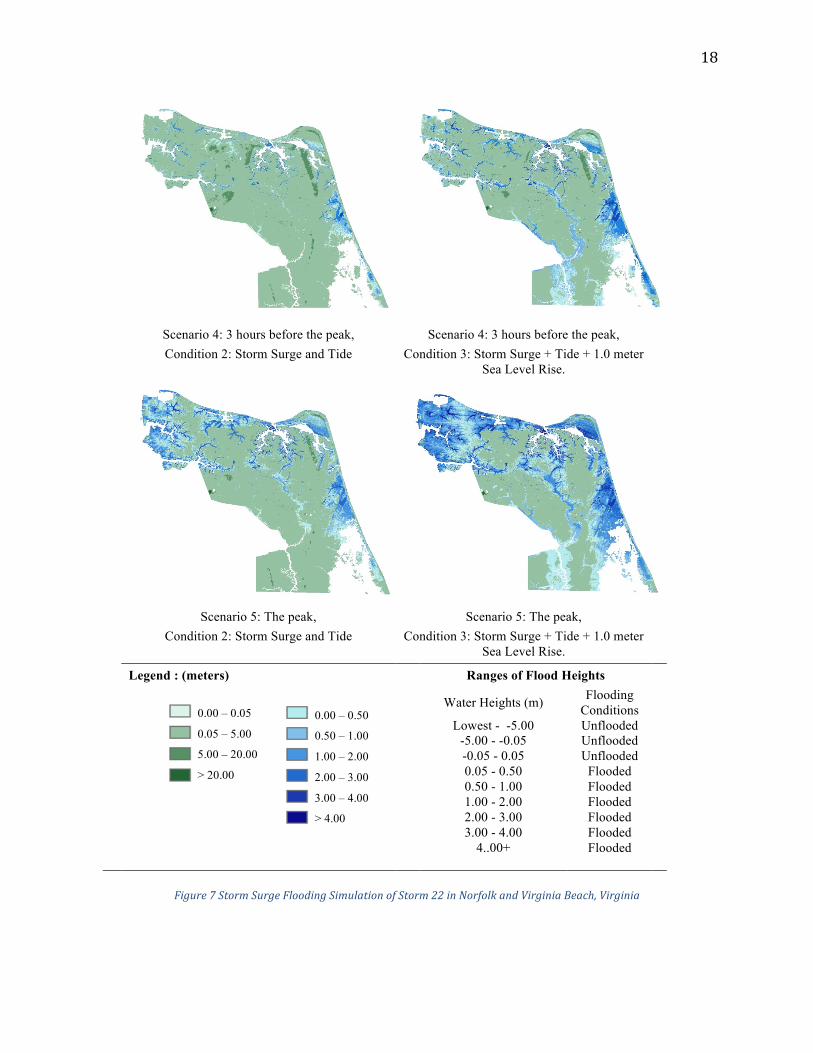
2.5.3 Connectivity Analysis Network connectivity for this study was demonstrated in terms of miles of flooded roads and isolated networks where areas were physically separated from other areas due to flooded (impassible) roads. After identifying disconnected areas, polygons were created for inaccessible areas to be visually identified as the isolated areas with centroids. The number of isolated networks was determined based on the centroids of unflooded areas. 2.6 Results Figure 7 presents the spatial outputs of the time period flooding scenarios for conditions 2 and 3 with a color-coded technique to indicate the severity level. (Note: The results for condition 1 was visually similar to condition 2.) Table 2 summarizes the comparison of the two conditions for each time period. Moreover, the connectivity which can be shown as isolated sub-networks on the GIS maps are summarized in Figure 8. The number of isolated sub-networks, indicated in Figure 9, was used as an indication of the severity level of the storm surge flooding.

17

Scenario 1: 12 hours before the peak, Condition 2: Storm Surge and Tide

Scenario 1: 12 hours before the peak, Condition 3: Storm Surge + Tide + 1.0 meter

Sea Level Rise.



Sea Level Rise.


Scenario 3: 6 hours before the peak, Condition 3: Storm Surge + Tide + 1.0 meter Sea Level

Rise.

18



Sea Level Rise.

Scenario 5: The peak, Condition 2: Storm Surge and Tide

Scenario 5: The peak, Condition 3: Storm Surge + Tide + 1.0 meter

Sea Level Rise.

Legend : (meters) Ranges of Flood Heights

Water Heights (m) Flooding Conditions

Lowest - -5.00 Unflooded -5.00 - -0.05 Unflooded -0.05 - 0.05 Unflooded 0.05 - 0.50 Flooded 0.50 - 1.00 Flooded 1.00 - 2.00 Flooded 2.00 - 3.00 Flooded 3.00 - 4.00 Flooded 4..00+ Flooded

Figure7StormSurgeFloodingSimulationofStorm22inNorfolkandVirginiaBeach,Virginia

0.00 – 0.05

0.05 – 5.00

5.00 – 20.00

> 20.00

0.00 – 0.50

0.50 – 1.00

1.00 – 2.00

2.00 – 3.00

3.00 – 4.00

> 4.00

19

Table2ResultsofGIS-basedFloodingAnalysisforAllScenarios

Scenario Condition 2 Condition 3

Flooded Area (%)

Highest Water Height (meters)

Flooded Area (%)

Highest Water Height (meters)

1 4 1.5 22 2.5

2 7 2.3 25 3.0

3 6 2.7 25 3.2

4 9 3.2 26 3.8

5 27 4.5 52 5.2

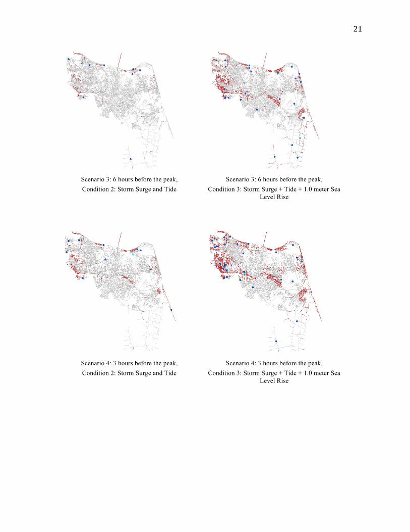
As shown in Table 2, for condition 2, the percentages of flooded areas ranged from 4% to 27% generally increasing with time. The percentage of flooded area expanded considerably in the three hours leading up to the peak. Condition 3 had higher percentages of flooded area compared to condition 2. In the first four time periods, the percentages fell in the range of 22%-26% compared to the range of 4%-9% for condition 2, which indicated a noticeable effect of 1.0 m of sea level rise. During the peak period under condition 3, more than half of the study area was flooded, whereas only 27% of the area was inundated under condition 2. Figure 7 shows the water heights of all flooding scenarios visualized using graduated colors to represent differences in magnitude of water heights. Blue represents the flooded areas, while green indicates the unflooded areas. The darker blue colors located near water bodies illustrate high water surfaces above the ground. According to Table 2, the range of the highest water level values for the scenarios of condition 2 is 1.5 - 4.5 m. They are less than those of condition 3, which rise from 2.5 m to 5.2 m. The flooded roads were identified for every scenario of both conditions. Most of the GIS maps also show that the roads would likely be inundated at the range of water heights of 2-5 meters. As shown in Figure 8, the whole network cannot be traversed due to the isolated sub-networks. As shown in Figure 9, for condition 2, the number of isolated networks was 5 for scenario 1 (12 hours before peak) and then increased to 11 for scenario 4 (3 hours before peak). During the peak period, the number approximately doubled. The results of condition 3 showed an increased number of isolated networks. There were 13 isolated networks for scenario 1 (12 hours before the peak), Similar to the results of condition 2, the increasing trend was observed for scenario 2-5 of condition 3. Condition 3 (with sea level rise) had more adverse impacts than condition 2 because the number of isolated networks for condition 2 was smaller than those of condition 3 for every time scenario.

20


Scenario 1: 12 hours before the peak, Condition 3: Storm Surge + Tide + 1.0 meter Sea

Level Rise



Level Rise

21



Level Rise



Level Rise

22

Scenario 5: The peak, Condition 2: Storm Surge and Tide

Scenario 5: The peak, Condition 3: Storm Surge + Tide + 1.0 meter Sea

Level Rise

Figure8IsolatedNetworksExposedtoStormSurgeandSeaLevelRise,NorfolkandVirginiaBeach,Virginia

Figure9NumberofIsolatedNetworksforAllScenarios

Table 3 also demonstrated the length of flooded roads under the effects of storm surge, tide and sea level rise. The maximum length of 894 miles was flooded during the peak period of flooding for condition 3, whereas 655 miles of roads were under water for condition 2. Moreover, the length

0

5

10

15

20

25

30

35

1 2 3 4 5

Num

ber

of Is

olat

ed N

etw

orks

Scenario

Condition 2

Condition 3

Unflooded Road

Flooded Road

Legend

23

of flooded roads for condition 3 increased by 600 miles in twelve hours before the peak from 294 to 894 miles because of a 1 meter sea level rise. Nevertheless, the increased length of 455 miles could be inundated in twelve hours before the peak for condition 2, and it can be noted for condition 2 that much more roads were inundated from within 3 hours before the peak from 255 to 655 miles (157 percent) compared to condition 3. The flooded roads were 547 miles in length at 3 hours before the peak of condition 3, and then were 894 in length at the peak. Moreover, the comparison of the flooded roads between conditions 2 and 3 for each scenario which was illustrated in Figure 10 can account for the impact of sea level rise on the network. Condition 3 gave rise to more flooded roads than condition 2 for every scenario. The 1 meter sea level rise brought about the increases in length of flooded roads ranging approximately from 100 to 350 miles for scenarios 1 to 5 of condition 3.

Table3LengthofFloodedRoadsinMilesforAllScenarios

Scenario Condition 2 Condition 3

Percent Increase (%)

Percent Increase (%)

1 200 294

2 220 10 409 40

3 227 4 466 14

4 255 13 547 18

5 655 157 894 64

Figure10ComparisonofLengthofFloodedRoads

0

100

200

300

400

500

600

700

800

900

1000

1 2 3 4 5

Len

gth

of F

lood

ed R

oads

(mile

s)

Scenario

Condition2

Condition3

24

2.7 Conclusions, Recommendations, and Future Research This chapter used water level time series data from the U.S. Army Corps of Engineers to determine flood depths and flooded areas, and to assess the network vulnerability of Norfolk and Virginia Beach to tropical storm surge for three conditions, including (1) the base condition with storms modeled on mean sea level with wave effects, but no sea level change or astronomical tides, (2) the base condition plus tide, and (3) the base condition plus tide and 1.0 meter of sea level rise. One storm (ID 22) of 1,050 synthetic tropical storms was selected for this study to illustrate the approach and effects. A SQL database was used to collect the water levels from all the save points throughout the study area for time snapshots. These water levels were used with GIS techniques to visualize and analyze flooding. The GIS methodology was based on the overlay analysis and IDW technique to show the water surface on the flood maps which were later transformed to flood depths. For the connectivity analysis, the number of isolated sub-networks was calculated based on the connectivity analysis to illustrate how much the network would be disconnected due to the effect of storm surge and sea level rises. The highest water level values for the scenarios of condition 2 ranged from 1.5 to 4.5 meters, while those of condition 3 fell between 2.5 and 5.2 meters. Based on the flood heights of the two conditions, the flooding events of condition 3 were worse compared to those of condition 2 due to the one-meter sea level rise. Furthermore, some roads would likely be inundated at the range of water heights of 2-5 meters. This implication of flood risk areas can be analyzed in context of the size of flood-risk areas for different scenarios of storm surge and sea level. For condition 2 under storm surge and tides, the flood risk area expansion (4% to 27%) would be less than that of condition 3 with the range to 22% to 26% before the peak period, and more than half of the flooded area during the peak period. Therefore, the significant increases in the size of flood-risk areas under 1 meter of sea level rise demonstrated that sea level rise increases the network vulnerability, answering research question 1. These results led to recommendations for sea level rise adaptation strategies for this area (see for example Chapter 4), as well as for evacuation plans tailored to these areas. The number of isolated networks for every scenario of condition 3 was dramatically greater than that of condition 2. That is, a greater number of smaller isolated networks were generally found in condition 3 compared to the results of condition 2. It is obvious that sea level rise had an impact on this study area, which helped provide the answer to research question 2 since many more isolated networks were found for condition 3. Sea level rise causes the expansion of the flood-risk areas affected by storm surges and tides under condition 2, and result in higher flood depths. It is likely that more people would be stuck in the inundated areas, so it is necessary that residents evacuate before the flooding event could be worse. Furthermore, results from the connectivity analysis in Figure 9 supported the above belief because the number of isolated sub-networks substantially rose by around 50% when the effect of sea level rise was considered in the analysis. This could mean that residents would face more flooded areas with sea level rise for the same time period and would thus need to clear the network earlier during an evacuation.

25

Moreover, the length of flooded roads could be used to measure the network connectivity. Similarly, the increasing trends of the length of flooded roads can be expected for both conditions. The percent increases in the length of flooded roads from one period to the next vary from 4 to 157 for condition 2, and from 14 to 64 for condition 3. The flooded roads of condition 3 were approximately 100 to 200 miles longer than those of condition 2 during the first two scenarios. Afterwards, the length of the flooded roads for condition 3 was 300 to 350 miles greater than that of condition 2. This research can be improved in three aspects. First, the vulnerability to storm surge and sea level rise should be assessed for other elements of the disaster, such as people, economy (business) and health because all the elements are inevitably affected when the storm reaches the area, and the disaster planning and management include different elements in the system. For example, the estimation of vulnerable populations and business exposure to flood risk could support resource allocation and plans for the provision of emergency services. Second, the evacuation demand could be included in the future work because the number of affected people is directly related to evacuation needs. The clearance of the road network is expected for supporting substantial evacuation. Third, this work can be extended to an interactive web-based flood hazard system for users to access these datasets and select their own areas because the study area has a variety of characteristics. Some functions, combined with a user friendly interface, could improve flood risk management.

26

3 Comparison of Microscopic and Mesoscopic Traffic Modeling Tools for Evacuation Analysis

3.1 Problem In the United States in 2015, evacuations as the result of natural or man-made disasters cost insurance companies $16.1 billion to cover the damages (Bellomo, Clarke et al. 2016). In the event of a disaster, an evacuation process is needed to move people away from risk to the nearest safe zone. A large-scale evacuation depends on many factors, such as the network infrastructure that is used during the evacuation and the number of vehicles that are used by evacuees. Ideally, an effective evacuation process will minimize the total evacuation processing time and maximize the number of people that survive. Several evacuation models have been developed and used to enhance the performance of evacuation processes. Alsnih and Stopher (2004) describe different traffic simulation models and emergency evacuation models, including micro simulation models, which have become more popular in evacuation planning. Microscopic simulation tools can track each individual vehicle behavior (Balmer, Axhausen et al. 2006). Therefore, decision-making of individuals can be explained. MATSim is an agent-based model that can be used to model an evacuation scenario (Rieser, Dobler et al. 2014). MATSim has been applied as an evacuation simulation model for many regions (Lämmel, Rieser et al. 2008, Lämmel 2011, Durst, Lämmel et al. 2014). For example, MATSim was used to analyze an evacuation plan in Hamburg, Germany. the analysis showed that the current evacuation plan was sufficient to save people’s lives (Durst, Lämmel et al. 2014). MATSim was also applied to simulate the evacuation of large-scale pedestrian , and the queue simulation that using by MATSim was able to capture the congestion effects of bottlenecks (Lämmel, Rieser et al. 2008). MATSim was used to find the best evacuation routes for escaping a tsunami (Lämmel 2011). The authors found that the Nash equilibrium routing approach is better than the shortest path routing approach. Studies have compared MATSim with other software, such as VISUM (a transportation planning system (Piatkowski and Maciejewski 2013)). MATSim produced a shorter travel time than VISUM. This result was not surprising since MATSim was free of congestion because it’s the re-planning stage is able to change vehicle routes to decrease congestion problems. MATSim and EMME/2 (a complete travel demand modeling system (EMME 2008)) have also been compared (Gao, Balmer et al. 2010). Results showed that MATSim had better performance in terms of travel time and link speed. Moreover, MATSim was more realistic in terms of capturing congestion in the network. INTEGRATION, which is a microscopic traffic assignment model (Van Aerde and Rakha 2007, Van Aerde and Rakha 2007), has been used to optimize network traffic flows over time to improve evacuation planning (Chamberlayne 2011). INTEGRATION has also been compared with other software, such as VISSIM (PTV 2007). Both INTEGRATION and VISSIM are based on modeling

27

a signalized approach. INTEGRATION includes a behavioral model, while VISSIM includes a statistical stop/go probability model (Gao 2008). This report evaluates INTEGRATION and MATSim for different evacuation scenarios and compares the performance of the two models. This report is organized into four additional sections. The first section describes the two models that were used to evaluate the performance of the evacuation scenario. The second section describes the study area, which is a section of Knoxville, Tennessee. The second section also describes the simulation network and demand file construction and calibration. The third section shows the results of the models. The fourth section presents the conclusions and any future work. 3.2 Approach Therefore, the objective of this research is to develop the performance of evacuation scenario using two different models; INTEGRATION and MATSim. The research team aims to demonstrate the comparisons for two models. 3.3 Methodology Several evacuation simulation models have been developed to predict the performance of an evacuation scenario in a specific region, such as VISSIM (Boden, Buzna et al. 2007, Gao 2008, Qiao, Ge et al. 2009), TRANSIMS (Cetin, Nagel et al. 2002, Balmer, Axhausen et al. 2006), and AIMSUN (Algers, Bernauer et al. 1997). This section describes the two models that were used in terms of evaluating the performance of the evacuation scenario. These models represent two different genres of models. INTEGRATION is a trip-based model, and MATSim is an agent-based model. 3.3.1 INTEGRATION Simulation Model INTEGRATION is a microscopic traffic assignment simulation model. It computes a number of measures of effectiveness (MOEs) after finishing the simulation, such as total delay, the number of stops, fuel consumption, and emissions. INTEGRATION guarantees high-accuracy results by tracking each individual vehicle every 0.1 s. This allows detailed analyses of lane-changing movements and shockwave propagations. The model uses the Rakha-Pasumarthy-Adgerid model (RPA) of car following to depict the relationship between a vehicle and the vehicle ahead of it. INTEGRATION computes the vehicle speed by taking into account a vehicle dynamics model that considers the resultant force between the vehicle’s tractive effort and three resistance forces, including aerodynamic resistance, grade resistance, and the rolling resistance. It can model many features, such as adaptive traffic signal optimization, eco-routing, speed harmonization, fuel consumption, and emissions. The calibration of the INTEGRATION software entails two calibration efforts, namely calibration of the traffic demand and calibration of the network supply. 3.3.1.1 Traffic Simulation Model Input The input data for INTEGRATION are divided into fundamental data and advanced data. Fundamental data are essential to run the software. Advanced data are optional depending on which file are you interested in.

28

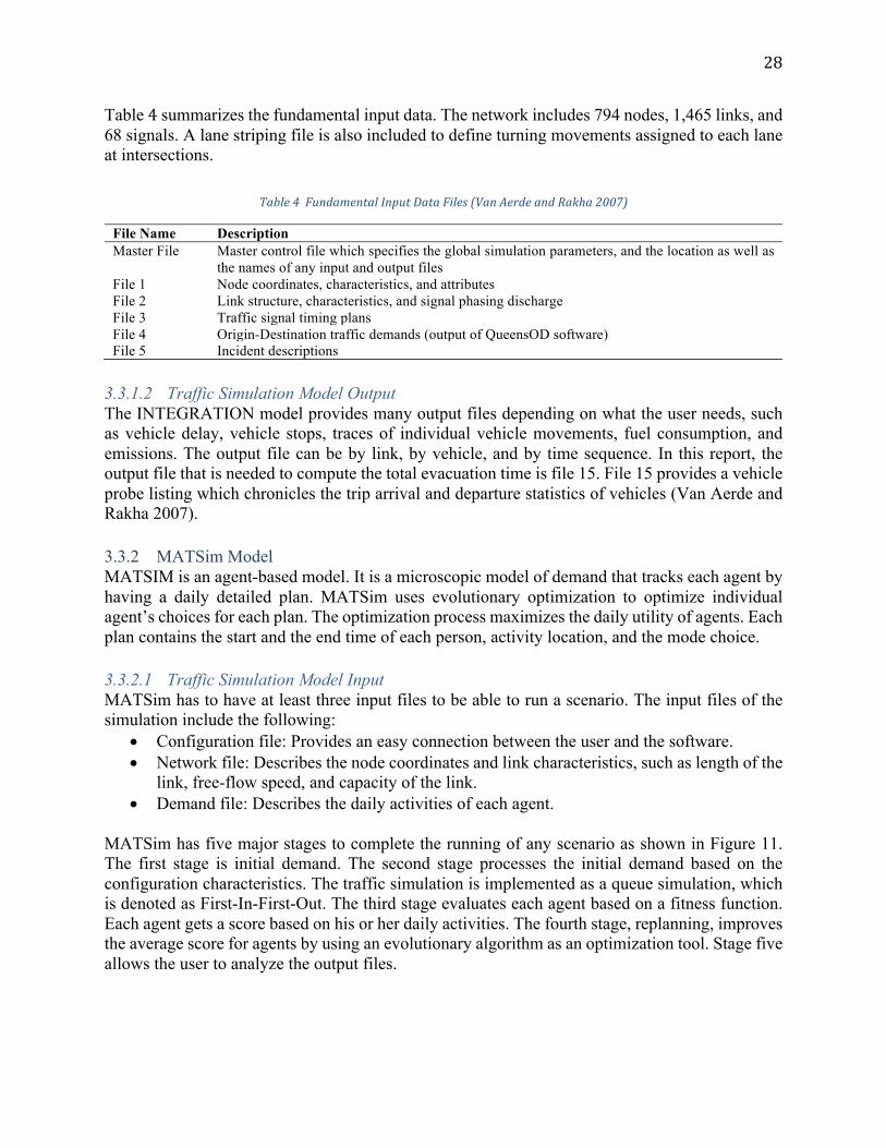
Table 4 summarizes the fundamental input data. The network includes 794 nodes, 1,465 links, and 68 signals. A lane striping file is also included to define turning movements assigned to each lane at intersections.

Table4FundamentalInputDataFiles(VanAerdeandRakha2007)

File Name Description Master File Master control file which specifies the global simulation parameters, and the location as well as

the names of any input and output files File 1 Node coordinates, characteristics, and attributes File 2 Link structure, characteristics, and signal phasing discharge File 3 Traffic signal timing plans File 4 Origin-Destination traffic demands (output of QueensOD software) File 5 Incident descriptions 3.3.1.2 Traffic Simulation Model Output The INTEGRATION model provides many output files depending on what the user needs, such as vehicle delay, vehicle stops, traces of individual vehicle movements, fuel consumption, and emissions. The output file can be by link, by vehicle, and by time sequence. In this report, the output file that is needed to compute the total evacuation time is file 15. File 15 provides a vehicle probe listing which chronicles the trip arrival and departure statistics of vehicles (Van Aerde and Rakha 2007). 3.3.2 MATSim Model MATSIM is an agent-based model. It is a microscopic model of demand that tracks each agent by having a daily detailed plan. MATSim uses evolutionary optimization to optimize individual agent’s choices for each plan. The optimization process maximizes the daily utility of agents. Each plan contains the start and the end time of each person, activity location, and the mode choice. 3.3.2.1 Traffic Simulation Model Input MATSim has to have at least three input files to be able to run a scenario. The input files of the simulation include the following:

• Configuration file: Provides an easy connection between the user and the software. • Network file: Describes the node coordinates and link characteristics, such as length of the

link, free-flow speed, and capacity of the link. • Demand file: Describes the daily activities of each agent.

MATSim has five major stages to complete the running of any scenario as shown in Figure 11. The first stage is initial demand. The second stage processes the initial demand based on the configuration characteristics. The traffic simulation is implemented as a queue simulation, which is denoted as First-In-First-Out. The third stage evaluates each agent based on a fitness function. Each agent gets a score based on his or her daily activities. The fourth stage, replanning, improves the average score for agents by using an evolutionary algorithm as an optimization tool. Stage five allows the user to analyze the output files.

29

Figure11StagesofaMATSimsimulation(MarcelRieserandGregorL�ammel2014)

3.4 Study Area A total of 11 scenarios were evaluated for an evacuation of a section near Knoxville, Tennessee (Figure 12). This area could be exposed to a natural disaster such as flooding that would impact both communities and transportation infrastructure. The definitions of these scenarios are presented in Table 5. These scenarios were created based on seasonal variations, day of the week, adverse weather, roadway impacts, and the peak construction workforce in the city. The differences between scenarios are in road capacity, free-flow speed, jam density, and speed at capacity.

Figure12Knoxville,TN(Source:GoogleMaps).

30

Table5Definitionsofthe11Scenarios

Scenario Description 1 Typical normal weather, midweek daytime period in summer 2 Adverse weather, daytime midweek period in summer 3 Typical normal weather, weekend daytime period in summer 4 Typical normal weather, midweek and weekend evening period in summer 5 Typical normal weather, midweek daytime period in winter 6 Adverse weather, midweek daytime period in winter 7 Typical normal weather, weekend daytime period in winter 8 Typical normal weather, midweek and weekend evening period in winter 9 Different conditions that may impact a roadway segment such as vehicle accidents, typical normal

weather, midweek daytime period in summer 10 Typical normal weather, midweek daytime period in summer; assumes that roads have the peak

number of construction workers on-site 11 Typical normal weather, midweek daytime period in summer; this scenario predicts the future demand 3.4.1 Simulation File Construction and Calibration The road network needed for the simulation input files was constructed from a Geographic Information System (GIS) shapefile. A detailed field survey was conducted to obtain the characteristics of the primary roadways and validate the original coding of the network. Roadway characteristics obtained during the field survey included the number of lanes, lane width, intersection configuration, lane channelization and striping, geometrics (curves and lengths), speed limit, and other necessary characteristics.

The demand file is composed of two parts: background/pass-through traffic and evacuation traffic flow. Background and pass-through traffic will exist at the time an order to evacuate is issued. To estimate the background and pass-through traffic, QueensOD (Rakha 2002), a software application developed by the Virginia Tech Transportation Institute (VTTI), was used. QUEENSOD is a model for estimating origin-destination (O-D) traffic demands based on observed link traffic flows, observed link turning movement counts, link travel times, and, potentially, additional information on drivers’ route choices. QueensOD iteratively minimizes errors between observed link volumes to estimated link flow using a Least Relative Error (LRE) model and generates an O-D matrix. The latest published traffic statistics, provided by the Tennessee Department of Transportation (http://www.tdot.state.tn.us/traffichistory), were used to as the input data for QueensOD. The count stations and network in the area are shown in Figure 13.

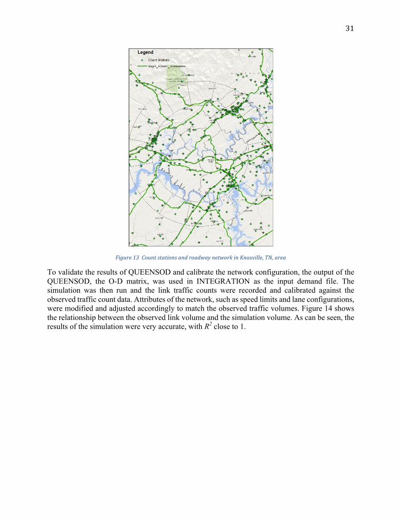
31

Figure13CountstationsandroadwaynetworkinKnoxville,TN,area

To validate the results of QUEENSOD and calibrate the network configuration, the output of the QUEENSOD, the O-D matrix, was used in INTEGRATION as the input demand file. The simulation was then run and the link traffic counts were recorded and calibrated against the observed traffic count data. Attributes of the network, such as speed limits and lane configurations, were modified and adjusted accordingly to match the observed traffic volumes. Figure 14 shows the relationship between the observed link volume and the simulation volume. As can be seen, the results of the simulation were very accurate, with R2 close to 1.

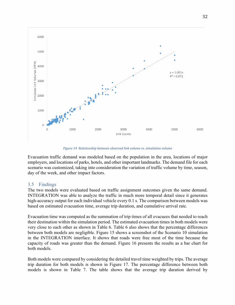
32

Figure14Relationshipbetweenobservedlinkvolumevs.simulationvolume

Evacuation traffic demand was modeled based on the population in the area, locations of major employers, and locations of parks, hotels, and other important landmarks. The demand file for each scenario was customized, taking into consideration the variation of traffic volume by time, season, day of the week, and other impact factors. 3.5 Findings The two models were evaluated based on traffic assignment outcomes given the same demand. INTEGRATION was able to analyze the traffic in much more temporal detail since it generates high-accuracy output for each individual vehicle every 0.1 s. The comparison between models was based on estimated evacuation time, average trip duration, and cumulative arrival rate. Evacuation time was computed as the summation of trip times of all evacuees that needed to reach their destination within the simulation period. The estimated evacuation times in both models were very close to each other as shown in Table 6. Table 6 also shows that the percentage differences between both models are negligible. Figure 15 shows a screenshot of the Scenario 10 simulation in the INTEGRATION interface. It shows that roads were free most of the time because the capacity of roads was greater than the demand. Figure 16 presents the results as a bar chart for both models. Both models were compared by considering the detailed travel time weighted by trips. The average trip duration for both models is shown in Figure 17. The percentage difference between both models is shown in Table 7. The table shows that the average trip duration derived by

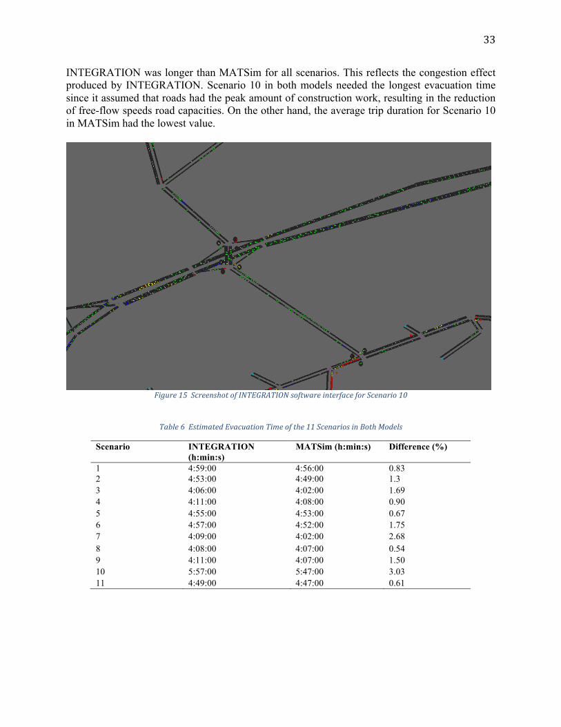
33

INTEGRATION was longer than MATSim for all scenarios. This reflects the congestion effect produced by INTEGRATION. Scenario 10 in both models needed the longest evacuation time since it assumed that roads had the peak amount of construction work, resulting in the reduction of free-flow speeds road capacities. On the other hand, the average trip duration for Scenario 10 in MATSim had the lowest value.

Figure15ScreenshotofINTEGRATIONsoftwareinterfaceforScenario10

Table6EstimatedEvacuationTimeofthe11ScenariosinBothModels

Scenario INTEGRATION (h:min:s)

MATSim (h:min:s) Difference (%)

1 4:59:00 4:56:00 0.83 2 4:53:00 4:49:00 1.3 3 4:06:00 4:02:00 1.69 4 4:11:00 4:08:00 0.90 5 4:55:00 4:53:00 0.67 6 4:57:00 4:52:00 1.75 7 4:09:00 4:02:00 2.68 8 4:08:00 4:07:00 0.54 9 4:11:00 4:07:00 1.50 10 5:57:00 5:47:00 3.03 11 4:49:00 4:47:00 0.61

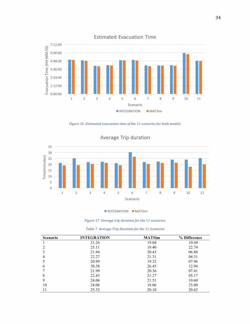
34

Figure16Estimatedevacuationtimeofthe11scenariosforbothmodels.

Figure17Averagetripdurationforthe11scenarios.

Table7AverageTripDurationforthe11Scenarios

Scenario INTEGRATION MATSim % Difference 1 21.26 19.04 10.44 2 25.11 19.40 22.74 3 21.94 20.43 06.88 4 22.27 21.31 04.31 5 20.99 19.32 07.96 6 30.38 26.45 12.94 7 21.99 20.36 07.41 8 22.43 21.27 05.17 9 24.06 21.51 10.60 10 24.08 18.06 25.00 11 25.32 20.10 20.62

0:00:00

1:12:00

2:24:00

3:36:00

4:48:00

6:00:00

7:12:00

1 2 3 4 5 6 7 8 9 10 11

Evacuatio

nTime(HH:MM:SS)

Scenario

EstimatedEvacuationTime

INTEGRATION MATSim

05101520253035

1 2 3 4 5 6 7 8 9 10 11

Time(minutes)

Scanario

AverageTripduration

INTEGRATION MATSim

35

The cumulative arrival rate of both models was part of the comparison. The cumulative arrival rates in Figure 18, Figure 19, and Figure 20 show the number of evacuees with time. In all scenarios, there was a 45-minutes background traffic simulation before the evacuation traffic (pass-through) stimulation started. Figure 18 and Figure 19 show the summer and winter season trends, respectively, by varying the daytime, weather, and the day of week. Figure 20 shows different scenarios of roadway impact, peak construction, and future prediction.

36

Figure18Summerseasonscenarios(a)normalweathermidweekdaytime(b)adverseweathermidweekdaytime(c)normalweatherweekenddaytime(d)normalweather

midweekandweekendeveningperiod

0

20

40

60

80

100

0:00:00 1:00:00 2:00:00 3:00:00 4:00:00 5:00:00 6:00:00 7:00:00

Num

berofVehicles Thousands

Time(HH:MM:SS)

CumulativeArrival

MATSim INTEGRATION(a)

0

20

40

60

80

100

0:00:00 1:00:00 2:00:00 3:00:00 4:00:00 5:00:00 6:00:00 7:00:00

Num

berofVehicles

Thousands

Time(HH:MM:SS)

CumulativeArrival

MATSim INTEGRATION(b)

0

20

40

60

80

100

0:00:00 1:00:00 2:00:00 3:00:00 4:00:00 5:00:00 6:00:00 7:00:00

Num

berofVehicles

Thousands

Time(HH:MM:SS)

CumulativeArrival

MATSim INTEGRATION(c)

0

20

40

60

80

0:00:00 1:00:00 2:00:00 3:00:00 4:00:00 5:00:00 6:00:00 7:00:00Num

berofVehicles

Thousands

Time(HH:MM:SS)

CumulativeArrival

MATSim INTEGRATION(d)

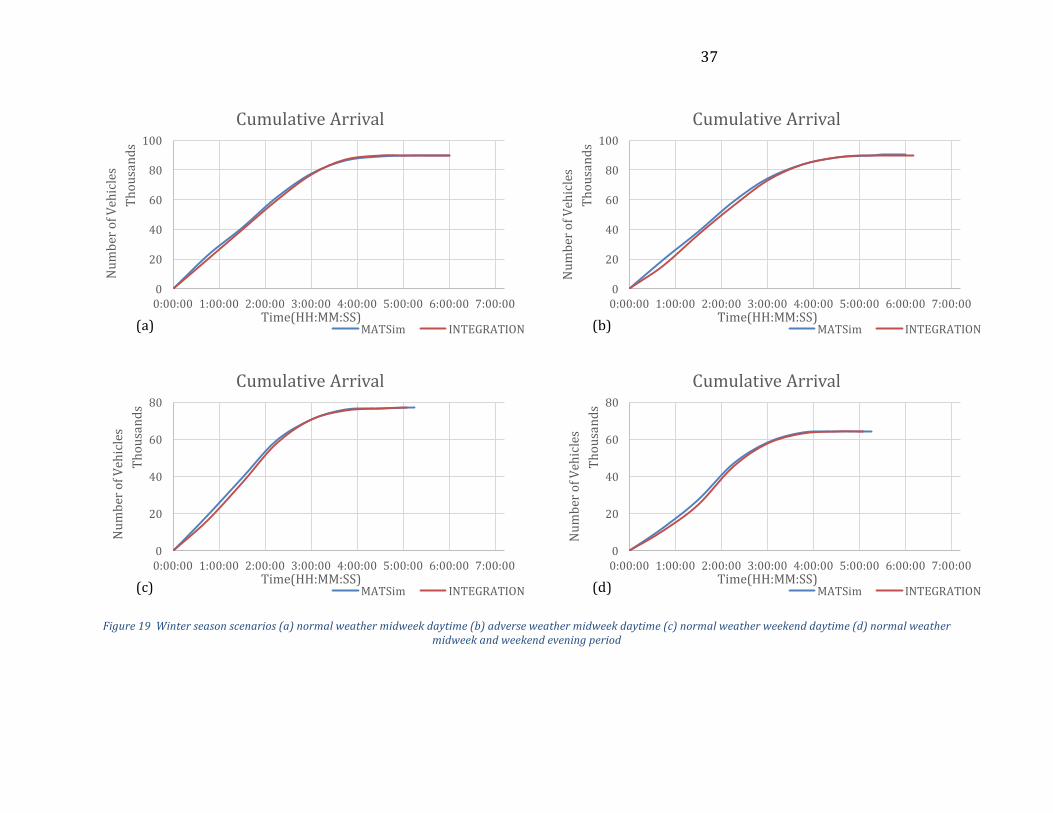
37

Figure19Winterseasonscenarios(a)normalweathermidweekdaytime(b)adverseweathermidweekdaytime(c)normalweatherweekenddaytime(d)normalweathermidweekandweekendeveningperiod

0

20

40

60

80

100

0:00:00 1:00:00 2:00:00 3:00:00 4:00:00 5:00:00 6:00:00 7:00:00

Num

berofVehicles

Thousands

Time(HH:MM:SS)

CumulativeArrival


0

20

40

60

80

100

0:00:00 1:00:00 2:00:00 3:00:00 4:00:00 5:00:00 6:00:00 7:00:00

Num

berofVehicles

Thousands

Time(HH:MM:SS)

CumulativeArrival


0

20

40

60

80

0:00:00 1:00:00 2:00:00 3:00:00 4:00:00 5:00:00 6:00:00 7:00:00

Num

berofVehicles

Thousands

Time(HH:MM:SS)

CumulativeArrival


0

20

40

60

80

0:00:00 1:00:00 2:00:00 3:00:00 4:00:00 5:00:00 6:00:00 7:00:00Num

berofVehicles

Thousands

Time(HH:MM:SS)

CumulativeArrival

MATSim INTEGRATION(d)

38

Figure20Differentscenarios(a)roadwayimpact(b)peakconstruction(c)futurepurposes

0

20

40

60

80

100

0:00:00 1:00:00 2:00:00 3:00:00 4:00:00 5:00:00 6:00:00 7:00:00

Num

berofVehicles

Thousands

Time(HH:MM:SS)

CumulativeArrival


0

20

40

60

80

100

0:00:001:00:002:00:003:00:004:00:005:00:006:00:007:00:00

Num

berofVehicles

Thousands

Time(HH:MM:SS)

CumulativeArrival


0

20

40

60

80

100

120

0:00:00 1:00:00 2:00:00 3:00:00 4:00:00 5:00:00 6:00:00 7:00:00

Num

berofVehicles

Thousands

Time(HH:MM:SS)

CumulativeArrival


39

INTEGRATION provides additional output files that related with computing the Measure of Effectiveness (MOE) such as travel time, delay, fuel consumption, and emissions. Table 8 contains the output of MOE’s for all scenarios.

Table8MeasureofEffectivenessforthe11Scenarios

Scenario 1 2 3 4 5 6 7 8 9 10 11 Travel Time

1278.8 1504.5 1312.8 1352.1 1298.2 1820.6 1360.3 1342.8 1399.2 1433 1495

Delay (sec/veh)

502.1 626.2 577.6 645.1 527.7 672.7 606 627.1 625.5 592.9 551.1

Fuel (l/veh)

1.8 1.7 1.8 1.7 1.8 1.7 1.8 1.7 1.8 1.8 1.8

HC (g/veh)

5.6 3.8 5.5 5.0 5.6 2.3 5.5 5.0 5.5 5.7 5.9

NOx (g/veh)

135.2 86.6 133.4 117.6 135.5 42.0 131.8 117.9 132.9 137.4 142.4

CO2 (g/veh)

3883.3 3872.7 3944.6 3861.0 3915.4 3821.5 3962.5 3845.2 4000.2 3983 4047.1

3.6 Conclusions and Recommendations This report compared INTEGRATION and MATSim for modeling different evacuation scenarios. The models were compared based on the estimated evacuation time, average trip duration, and cumulative arrival plot. The estimated evacuation times of both INTEGRATION and MATSim were close to each other since the demand of all scenarios was less than the capacity of network. The evaluation showed a difference between the two models in the average trip duration. In INTEGRATION, the average trip duration increased with increasing traffic demand levels and decreasing roadway capacities. On the other hand, the average trip duration using MATSim decreased with increasing total travel time. The trends for the cumulative arrival times for both were close to each other. MATSim served more vehicles than INTEGRATION did at the beginning of the stimulation. After that, both models served the same number of vehicles and these trends become closer to each other. These results seem to demonstrate that a tool like MATSim may produce erroneous conclusions if network-wide average results are desired. Future considerations is to study the effect of congestion in the network by increasing the current demand. Results would show how each model can deal with queues of vehicles spilling back from link to link.

40

4 An Investigation of Climate Change Adaptation Case Study of the Hampton Boulevard Corridor in Norfolk, Virginia

Climate change, primarily sea level rise (SLR), has become a growing issue not one country faces but it is a global problem. Due to the change it is more evident and accelerating at a fast pace. There is an up-stir among scientists, researchers, and the government, who are trying to figure out what to do and how to adapt to these changes. These changes not only affect the environment but they also affect the economy, the livelihood of the population. If these problems are not dealt with or continue to be ignored, then there may not be anything left for the future generation. Therefore, since the environment is changing around us, it would only make sense to find ways by which different facilities such as transportation, in particular, can be improved or solutions implemented to increase the life cycle of these infrastructures. It is definitely essential that the authorities are prepared for the projected changes rather than waiting until the problems become too huge to be solved effectively. Over the years in Norfolk, the residences along with the authorities have been dealing with the constant issue of inundation of the area. As the years go by, the issue have been developing into a major problem, as funds are constantly been spent to fix the water damage as well as the fast deterioration of the infrastructure. In this research, the researcher would attempt to decipher how different methods or policies can be implemented for Norfolk to solve the problems they are faced with there. This is done by studying different methods, in terms of infrastructure, already established around the world and how it can be applied to the area if altered based on the geography (topography). Adaptation means to change the infrastructure where it becomes better suited to the changing environment. Additionally, use as a foundation was the Assessing Vulnerability and Risk of Climate Changes Effects on Transportation Infrastructure Report done. This report created a well detailed insight of the problems of Hampton Roads in general as well as how transportation infrastructure was access to determine its vulnerabilities towards the change of the climate. However, throughout the research of different strategies, it is ideal to note that the transportation sector is and will continue to be affected by climate change. However, it is better to attempt to adapt rather than ignore that the climate is changing drastically. 4.1 Literature Review 4.1.1 Background on Hampton Roads, Virginia The Hampton Roads is a metropolitan area of Southeastern Virginia which includes the independent cities of Chesapeake, Hampton, Newport News, Norfolk, Portsmouth, and Virginia Beach. Moreover, it is home for the various large Military bases stationed there, such as Marines, the Army, the Navy and the Coast Guard. The geographic makeup of the area is that it has been surrounded by smaller rivers that lead to two major rivers, James and Elizabeth River, which leads directly to the Atlantic Ocean. Hence, this provides a constant access for ships and boats. However, being surrounded by water has led to several issues such as sea level rise and high storm surge in the case of extreme weather. The Hampton Roads area in Virginia has experienced the highest rates of sea-level rise along the entire U.S. East Coast (Tompkins and DeConcini 2014). This is due to the consequence of climate change, which is affecting the infrastructure facilities, populations, homeowners of the affected area.

41

4.1.2 Background on Norfolk Within Hampton Roads, Norfolk is a city which mostly affected by all these changes. Miles of waterway that add to Norfolk’s charm are also a major threat in the era of increased global warming and relative rising sea levels, it’s odd and unique sinking ground (Fears 2015). It is very interesting to note that Norfolk is one of the oldest cities where it was constructed on wetlands and marsh to be conveniently accessible from the Chesapeake and Atlantic Ocean. Norfolk is also the home to the largest naval base on the East Coast and one of the largest in the world. Due to all of the present of the military base, Norfolk is very important city not only in Virginia, where 46% of the local economy comes from the Department of Defense spending (Tompkins and DeConcini 2014), but for the entire East Coast of United State as a major defense system. Moreover, Norfolk is highly populated, who experience intense damage during a severe weather. Flooding from powerful storm surge and high tide are not rare events that occur. Two noted major storms are 1933 Hurricane ‘Storm of the Century’ and Hurricane Isabel in 2003. Hurricane Isabel cost Virginia $925 million in damages to insured properties, while the 1933 Hurricane produced a storm surge in Hampton Roads about 21% higher than Hurricane Isabel. It was also noted that the rising of the sea level is the cause of the intensified storm surge. 4.1.3 Major Problems in Norfolk Global sea-level rise is caused by the thermal expansion caused by the warming of the oceans for water expands as it warms and the loss of land-based ice for instance glaciers and polar ice caps, due to increased melting. “When sea levels rise rapidly, as they have been doing, even a small increase can have devastating effects on coastal habitats. As seawater reaches farther inland, it can cause destructive erosion, flooding of wetlands, contamination of aquifers and agricultural soils, and lost habitat for fish, birds, and plants” (National Geographic 2015). In additional to that, infrastructure facilities has been greatly affected, for the facilities lifecycle has been reduce due to constant inundation and corrosion from salt water. This has become a major problem for Norfolk, which is now being closely monitored and projections have been made on the level expected to grow over the years. Floods exceeding today’s historic records are likely to take place within the next 20 to 30 years at sites across Virginia under mid-range sea level rise projections. Low-range projections lead to a more than even chance of floods exceeding five (5) feet above the high tide line in the same time frame for the Washington, DC and Hampton Roads areas, and by 2080 on the eastern shore and near the mouth of the Potomac Under high-range projections. At each site in this study there is a more than 90% chance of flooding above nine (9) feet this century (Kulp, Strauss et al. 2014). At the same token, sea level in Southeast Virginia is expected to rise between one and three plus feet by as early as 2060 (Virginia Institute of Marine Science 2013). This is clear evidence that the rising of the sea level has become a global issue which has caught the attention of all environmentalists, engineers, policy makers and government officials. It has become a major problem that has to be dealt with immediately to safeguard the livelihood of the population. The area [Hampton Roads] is also second only to New Orleans, LA, as the largest population center at risk from sea-level rise in the country (Tompkins and DeConcini 2014). Norfolk is not only experiencing sea level rise but over the years there has been clear evidence that that land is subsiding. Chesapeake Bay region at rates of 1.1 to 4.8 millimeters per year (mm/yr),

42

and subsidence continues today (Eggleston and Pope 2013). Eggleston and Pope continued to explain that this helps explain why the Hampton Roads region has the highest rates of sea-level rise on the Atlantic Coast of the United States. The cause of the land subsidence is due to ongoing geologic forces that contribute a net loss of elevation along with the plate tectonics and post-glacial isostatic adjustment (Boon et al., 2010). As a result land subsidence along with sea level rise has increase the risk of flooding in low-lying areas, which is evident through the occasionally inundation from high tide. The consequence of this problem spread across the scope of the economic, environmental and human health. 4.1.4 Fugro Atlantic Engineering Firm With all these issues becoming a huge issue, the government officials of Norfolk have consulted with a Dutch-based engineering firm, Fugro, to study the vulnerability of the area to high tides and intensified storm surges. Within the Fugro Atlantic Engineering Firm (2011) report, they noted that the City is located in a low-lying physiographic region, where the drainage gradients are limited and most of the City is below elevation +15 feet. Hence, majority of the City is susceptible to flooding from high tides, nor'easters, hurricanes, and other storm events. Moreover, the intensity of flooding ranges from nuisance flooding associated with high tides, to severe, albeit less frequent, flooding from hurricanes and major nor'easters, instance in November 2009. Fugro concluded that the construction of a floodwall, tide gate, a pump station and closure walls with a total capital cost of $47.4 Million would be the preferred choice for the City of Norfolk. Additionally the benefits of the plans were first, to improve access to Hospital during flood emergency, second, increase protection for the Freemason area and third, increase protection for the Light Rail. Another step taken to adapt to the changing sea level was the elevation of roads and streets, moreover, typically one street may cost $1.2 Million to be raised (Brangham 2012). Hence to elevate all roads of a city or to continue to do so will be very costly. On the other hand, Norfolk progression to adapting to these changes has earned it a spot on the Rockefeller Foundation’s 100 Resilient Cities Centennial Challenge. Cities selected receive technical support and resources for developing and implementing plans for urban resilience over the next three years. The main goal of this organization is to view the resilience that can enables cities to evaluate their exposure to specific shocks and stresses, as well as to develop a proactive and integrated plan to address those challenges, and to respond to them more effectively. In Norfolk’s case, the help in dealing with the increased flooding due to the results of rising sea level and land subsidence. 4.1.5 Adaptation Solutions Used Around the World 4.1.5.1 Case study of SMART in Malaysia In Malaysia, there has been estimated that at least 3.5 million people live on flood plains and are vulnerable to flood of varying probabilities it is also where much of the economic activities are concentrated (Weng Chan 1997). Malaysia has an equatorial climate with a constant high temperature and high humidity; however, they experience abundant heavy rainfall during the northeast monsoon season. The northeast monsoon season is between the months of October to March. Over the years, they have been affected by flash floods due to the intense precipitation and overflowing of the rivers during this season. A specific area where flash floods occur very frequent is in Kuala Lumpur, which was built along the flood plains of the Klang River. These flash floods have created an economic strain on the government upkeep funding for disaster relief for the population.

43

A solution that Malaysian Federal Government created to solve this issue, is the development of the Storm Management and Road Tunnel (SMART). This tunnel is the longest multipurpose tunnel in the world for it is a combined storm water and motorway tunnel. Along with the purpose of flood control, it will address the traffic congestion as well. As seen in figure one below, the way how it works is very interesting and unique, where it has three modes of operation. During mode one the storm water section remain close, however, during mode two and three, when the gate is triggered open, the water travels from the confluence Klang and Ampang rivers. The entire project costs US$515 million and has an expected benefit of US$1.58 billion of possible flood damage and prevent as well as up to US$1.26 billion savings from traffic congestion, all after a 30 year concession period (ITS International 2012). 4.1.5.2 Case study of the Flood Barriers in Holland, England and Louisiana In Holland, England and Louisiana all have something in common which is a large flood barrier in place to protect the surrounding area in case of the high tide, or storm surge during extreme weather. The Oosterscheldekering in Holland, the Thames Barrier in England and Inner Harbor Navigation Canal (IHNC) Lake Borgne Surge Barrier in Louisiana are all incredible and uniquely design to fit the different feature of their respective location. The storm barrier in Holland is the largest barrier in the Delta works which was developed in response to the widespread damage and loss of life due to the North Sea Flood of 1953. It was designed and expected to last for more than 200 years, with the total project cost of US$3.9 billion. The Thames Barrier is a unique flood control structure on the River Thames at Woolwich Reach in East London. It is 520 meters wide and protects London against storm and tidal surges, and rainfall swelling. The Thames was completed in 1882 with a life cycle until 2030 which is 148 years in total, costing US$835.1 million but US$2.5billion in today’s money value (Environment Agency 2015). It is also the 2nd largest flood defense barrier, behind the Oosterscheldkering in Holland. The IHNC was built and designed to reduce the risk of the storm damage to the areas that are most vulnerable to the areas in New Orleans, as well as, the risk of storm surge that has one percent chance of occurring in any given year or 100 year storm surge (US Army Corps of Engineers 2013). The total cost of the construction of the 1.8 miles barrier can be estimated to be $1.1 billion. The complexity of the barrier earned it several awards one of which was the 2014 Outstanding Civil Engineering Achievement from the American Society of Civil Engineers. 4.1.5.3 Case study of San Diego Bay In San Diego, the sea level had risen by just under one inch per decade on an average. San Diego is very similar to Norfolk, where it is a region that has a heavily invested coastal community and business. Moreover, it shares being a treasure asset; an anchor of the region’s tourism and military economies. And like Norfolk, they are experiencing the same problems with sea level rise, as there is expected a rate increase over the next couple years. The scientific community expects the rate of sea level rise will increase as higher concentrations of emissions will lead to faster warming and the melting of glaciers into the ocean. As a result, rising seas can lead to widespread flooding and erosion in low- lying areas, as well as impacts such as shifting habitats and rising water tables.

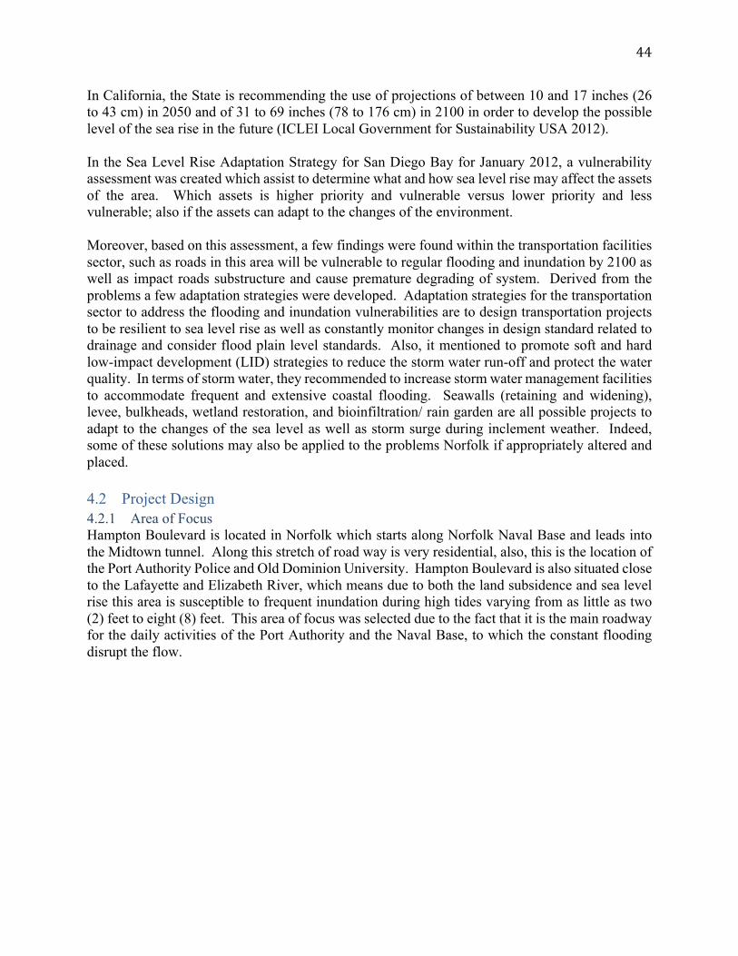
44

In California, the State is recommending the use of projections of between 10 and 17 inches (26 to 43 cm) in 2050 and of 31 to 69 inches (78 to 176 cm) in 2100 in order to develop the possible level of the sea rise in the future (ICLEI Local Government for Sustainability USA 2012). In the Sea Level Rise Adaptation Strategy for San Diego Bay for January 2012, a vulnerability assessment was created which assist to determine what and how sea level rise may affect the assets of the area. Which assets is higher priority and vulnerable versus lower priority and less vulnerable; also if the assets can adapt to the changes of the environment. Moreover, based on this assessment, a few findings were found within the transportation facilities sector, such as roads in this area will be vulnerable to regular flooding and inundation by 2100 as well as impact roads substructure and cause premature degrading of system. Derived from the problems a few adaptation strategies were developed. Adaptation strategies for the transportation sector to address the flooding and inundation vulnerabilities are to design transportation projects to be resilient to sea level rise as well as constantly monitor changes in design standard related to drainage and consider flood plain level standards. Also, it mentioned to promote soft and hard low-impact development (LID) strategies to reduce the storm water run-off and protect the water quality. In terms of storm water, they recommended to increase storm water management facilities to accommodate frequent and extensive coastal flooding. Seawalls (retaining and widening), levee, bulkheads, wetland restoration, and bioinfiltration/ rain garden are all possible projects to adapt to the changes of the sea level as well as storm surge during inclement weather. Indeed, some of these solutions may also be applied to the problems Norfolk if appropriately altered and placed. 4.2 Project Design 4.2.1 Area of Focus Hampton Boulevard is located in Norfolk which starts along Norfolk Naval Base and leads into the Midtown tunnel. Along this stretch of road way is very residential, also, this is the location of the Port Authority Police and Old Dominion University. Hampton Boulevard is also situated close to the Lafayette and Elizabeth River, which means due to both the land subsidence and sea level rise this area is susceptible to frequent inundation during high tides varying from as little as two (2) feet to eight (8) feet. This area of focus was selected due to the fact that it is the main roadway for the daily activities of the Port Authority and the Naval Base, to which the constant flooding disrupt the flow.

45

Figure21HighTideFloodingalongHamptonBoulevard

4.2.2 Methodology The occurrence of climate change has been in existence since the early 19th century progressing from a slow pace to an incredible very fast pace. Hence throughout the years, a vast number of reports and articles have been written on the topic and how it has affected different parts of the world. Once the broader picture was established the goal was now to determine some of the issues that Hampton roads face affect the infrastructure facilities over the years and how it will in the future. Land Subsidence, Sea Level Rise and Storm Surges are the main problems which affects the life span of transportation sectors. However, since this was such a broad topic as well as a large scope of an area to look at, with the help of Officials at Hampton Roads Transportation Planning Organization (HRTPO), it was narrowed down to concentrate on Hampton Boulevard in Norfolk; an area which has been experiencing clear evidence of all the issues previously stated, along with frequent flooding from high tide. HRTPO also provided documents which very specific to the general area of Hampton Roads but of Norfolk. Now that the problem was identified, it was ideal to determine the ways that this roadway was affected. The placement of this road, is situated where it is the route to access both the Norfolk Naval Base and the Police Authority as well as Old Dominion University. This means that when this road is inundated, or even worse, when the water slowly receded away, it would be impossible to maintain the daily traffic and activities along the route. The next step that was taken was to decipher which areas along this boulevard are more prone to inundation at the minimal height versus at the maximal height. With the help of Geographic Information Systems, this was done to gather the elevation of the area which revealed that majority, if not all, of this range is below sea level as seen below.

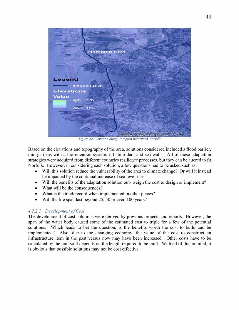
46

Figure22ElevationAlongHamptonBoulevard,Norfolk

Based on the elevations and topography of the area, solutions considered included a flood barrier, rain gardens with a bio-retention system, inflation dam and sea walls. All of these adaptation strategies were acquired from different countries resilience processes, but they can be altered to fit Norfolk. However, in considering each solution, a few questions had to be asked such as:

• Will this solution reduce the vulnerability of the area to climate change? Or will it instead be impacted by the continual increase of sea level rise.

• Will the benefits of the adaptation solution out- weigh the cost to design or implement? • What will be the consequences? • What is the track record when implemented in other places? • Will the life span last beyond 25, 50 or even 100 years?

4.2.2.1 Development of Cost The development of cost solutions were derived by previous projects and reports. However, the span of the water body caused some of the estimated cost to triple for a few of the potential solutions. Which leads to bet the question, is the benefits worth the cost to build and be implemented? Also, due to the changing economy, the value of the cost to construct an infrastructure item in the past versus now may have been increased. Other costs have to be calculated by the unit so it depends on the length required to be built. With all of this in mind, it is obvious that possible solutions may not be cost effective.

47

4.3 Solutions Analysis

Figure23PossibleSolutionsfortheHamptonBoulevardArea

48

4.3.1 Solution One - Flood Barrier One

Figure24FloodBarrierOneDesignfortheHamptonBoulevardAreaandInspiration

The first alternative is a flood barrier between Craney Island and Port Authority replicating the Maeslantkering Barrier in the Netherlands, as seen in Figure 24. The estimated distance between these two points is 1.53 miles (2.46 km) which triples the water span of the existing flood barrier. Moreover, due the distance estimated cost to construct a structure with similar principle is over two billion dollars. The highlighted feature of the design of this structure is that it is machine operated which will receive warning by the tidal system at Sewell Point when it should close at an anticipated increase of sea level, the minimum level will be set. When the gates are closing, it floats until it is securely closed where it will sink, by the weight of the water, into place where it will block the effects of high tide from inundating surrounding areas. Hence, during normal conditions, the barriers remain open for easy navigation of boats. Furthermore, based on the design and the nature of Port Authority and Craney Island, the construction of this Flood Barrier will require man made islands on either side as its base. With the help of the elevation map in Figure 22 the location of this barrier created the advantage of this solution is that the coast land, which is below the sea level, located after this barrier will be protected from frequent high tide and storm surge. This as a result this will minimize the necessity to implement smaller projects. Which bets the question, is it worth funding this large solution or use the same funding to develop smaller projects? However, the disadvantage of this project other than the cost to build is that if not efficiently maintained, it can result in malfunctioning or failure reducing its expected life cycle and very costly to fix.

4.3.2 Solution Two – Flood Barrier Two Flood barrier two is a flap type barrier which is operated by a hydraulic cylinder. It lays flat on the seabed beneath the Hampton Boulevard Bridge, but when a surge or high tide is predicted it will rise up to block the excess inflow of water. Moreover, when elevated it controls the fluctuation of water level, where it is kept calm. With this flood barrier, the marine traffic will not be disrupted on normal bases. This solution was inspired by the Thames Barrier in England and the Stamford Hurricane Barrier in Connecticut.

49

4.3.3 Solution Three – Bio-retention Rain Garden System

Figure25ExampleofBio-retentionBasin/RainGardenDesignfortheHamptonBoulevardArea.

How this system works is that stormwater is directed to the basins or garden and then it percolates through the system where it is treated by number of physical, chemical and natural process. The slow clean water is allowed to infiltrate and directed to nearby stormwater drainage. The idea is to direct flood water away from development and infrastructure slow run off and allow for re-location of the storm or flood water. Moreover, another ideal feature is that it purifies the water in the process, hence the nitrogen and phosphorus level and sediments will be reduces in the stormwater. However, due to the location of the road, these systems will have to be engineered to accommodate the salt water from high tide. The Blue Bird Park Stormwater Wetland Construction is expected to cost $84,500 which is already in place to be constructed. Also in Myrtle Park, there are plans for wetland restoration projected to be developed in the near future. Hence, these two locations are perfect to deposit water from some of the rain gardens along the Hampton Boulevard. The estimated cost for the development of rain gardens are $10 to $40 per square feet, which proposes to be placed along Hampton Boulevard in the medians and sideways.

In order to bring this solution to full effect, a policy can be implemented to encourage residents to construct rain gardens on their property. This way the rain gardens established along Hampton Boulevard will not be strained hence having a long life span if properly maintained as well. With all of this in place, this will improve the runoff time of storm water. 4.3.4 Solution Four – Flood Walls Flood wall is definitely an option where it is designed to protect the homes along the end of the Lafayette River but does not destroy the beautification of the area. The average cost to construct a floodwall with heights ranging from 3 to 10 feet is $110 to $410 per feet length. The disadvantage of this solution is that they have to be assembled very well so that water does not get through joints or steep through beneath it. 4.4 Limitations and Conclusion/Recommendations 4.4.1 Limitation There is always an uncertainty of the predictions of climate change which makes it difficult to develop adaptive strategies. Moreover, it is impossible to test the solutions; one can only

50

implement and monitor them to see if they are effective and good adaptive measures. If it is not, the funding spent to implement will be lost. However, if it does solve the existing problem there is a possibility that it may create a larger drawback. For instance, these solutions may work great and solve the problems along this corridor but it may cause major problems elsewhere in the Hampton Road region. Additionally, the selection and timing of the adaptive measures will greatly depend on the economical, political and environmental characteristics of Norfolk. Hence, a number of solutions could not work for Norfolk such as constructing a pond for temporary water storage because the area is so densely populated hence no land space available. Another limitation was the researcher was unable to locate the current drainage system route along Hampton Boulevard. However, the rain garden can be linked to the existing system or improved system which leads to both Blue Bird Park and Myrtle Park. 4.4.2 Conclusion To conclude, Hampton Boulevard in Norfolk Virginia serves a very important purpose as being the route to access the Naval Base, Port Authority, Old Dominion University and Midtown Tunnel. With this corridor being susceptible to high tide due to sea level rise and land subsidence, it is essential to develop potential solutions to adapt to the frequent inundation. The idea is to have a solution that is feasible and has a high cost benefit. On the first instincts is flood barrier one would be ideal because it will eliminate the need to develop smaller project for it protects a huge land space. However, what plays a huge role in determining the most suitable solution is the funding required to proceed with the construction. Hence, flood barrier two, flood wall and the biotention cell rain garden would possibly be more feasible and cost effective. As the world progresses and develops a better understanding of nature and the environment, new or modified infrastructure will also be developed to solve problems that it may face.

51

References Algers, S., E. Bernauer, M. Boero, L. Breheret, C. Di Taranto, M. Dougherty, K. Fox and J.-F.

Gabard (1997). "Review of micro-simulation models." Review Report of the SMARTEST project.

Alsnih, R. and P. Stopher (2004). "Review of procedures associated with devising emergency evacuation plans." Transportation Research Record: Journal of the Transportation Research Board(1865): 89-97.

Balmer, M., K. Axhausen and K. Nagel (2006). "Agent-based demand-modeling framework for large-scale microsimulations." Transportation Research Record: Journal of the Transportation Research Board(1985): 125-134.

Bell, M. G. (1995). "Alternatives to Dial's logit assignment algorithm." Transportation Research Part B: Methodological 29(4): 287-295.

Bellomo, N., D. Clarke, L. Gibelli, P. Townsend and B. Vreugdenhil (2016). "Human behaviours in evacuation crowd dynamics: from modelling to “big data” toward crisis management." Physics of life reviews 18: 1-21.

Bizimana, J. P. and M. Schilling (2009). Geo-Information Technology for Infrastructural Flood Risk Analysis in Unplanned Settlements: a case study of informal settlement flood risk in the Nyabugogo flood plain, Kigali City, Rwanda. Geospatial techniques in urban hazard and disaster analysis, Springer: 99-124.

Boden, M., L. Buzna and H. Weger (2007). "Simulation of Evacuation Scenarios in Urban Areas - Developing Tools for Modeling and Optimization of Evacuation Traffic Flows " TRANSCOM 2007: 7th.

Boon, J. D., J. M. Brubaker and D. R. Forrest (2010). "Chesapeake Bay land subsidence and sea level change." App. Mar. Sci. and Ocean Eng., Report 425: 1-73.

Brangham, W. (2012). "Rising Tide in Norfolk, Va." Retrieved June 17, 2015, from http://www.pbs.org/wnet/need-to-know/environment/rising-tide-in-norfolk-va/13739/.

Cetin, N., K. Nagel, B. Raney and A. Voellmy (2002). "Large-scale multi-agent transportation simulations." Computer Physics Communications 147(1-2): 559-564.

Chamberlayne, E. P. (2011). Optimal Evacuation Plans for Network Flows over Time Considering Congestion, Virginia Tech.

Cialone, M. A., T. C. Massey, M. E. Anderson, A. S. Grzegorzewski, R. E. Jensen, A. Cialone, D. J. Mark, K. C. Pevey, B. L. Gunkel and T. O. McAlpin (2015). North Atlantic Coast Comprehensive Study (NACCS) coastal storm model simulations: waves and water levels, DTIC Document.

D'este, G. and M. A. Taylor (2003). Network vulnerability: an approach to reliability analysis at the level of national strategic transport networks. The Network Reliability of Transport: Proceedings of the 1st International Symposium on Transportation Network Reliability (INSTR), Emerald Group Publishing Limited.

Deckers, P., W. Kellens, J. Reyns, W. Vanneuville and P. De Maeyer (2009). A GIS for flood risk management in Flanders. Geospatial techniques in urban hazard and disaster analysis, Springer: 51-69.

Durst, D., G. Lämmel and H. Klüpfel (2014). Large-scale multi-modal evacuation analysis with an application to Hamburg. Pedestrian and Evacuation Dynamics 2012, Springer: 361-369.

Eggleston, J. and J. Pope (2013). Land subsidence and relative sea-level rise in the southern Chesapeake Bay region, US Geological Survey.

52

EMME (2008). Users' Guide, Reference Manual, Prompt Manual v3.0; EMME/2 (1994) User's Manual.

Environment Agency. (2015, 12 June 2015). "The Thames Barrier." Retrieved June 27, 2015, from https://www.gov.uk/the-thames-barrier.

Fears, D. (2015). Built on Sinking Ground, Norfolk Tries to Hold Back Tide amid Sea-level Rise. The Washington Post.

Fletcher, C. H. (2009). "Sea level by the end of the 21st century: A review." Shore & beach 77(4): 4.

Freedman, A. (2012). "Top 5 Most Vulnerable U.S. Cities to Hurricanes." from http://www.climatecentral.org/news/top-5-most-vulnerable-us-cities-to-hurricanes.

Fugro Atlantic Engineering Firm (2011). Flood Mitigation Alternatives Evaluation The Hague Watershed, City of Norfolk, Department of Public Works.

Gao, W., M. Balmer and E. Miller (2010). "Comparison of MATSim and EMME/2 on greater Toronto and Hamilton area network, Canada." Transportation Research Record: Journal of the Transportation Research Board(2197): 118-128.

Gao, Y. (2008). Calibration and comparison of the VISSIM and INTEGRATION microscopic traffic simulation models, Virginia Tech.

ICLEI Local Government for Sustainability USA (2012). Sea Level Rise Adaptation Strategy for San Diego Bay, Public Agency Steering Committee.

Intergovernmental Panel On Climate Change (2007). "Climate change 2007: The physical science basis." Agenda 6(07): 333.

ITS International. (2012). "Success of Kuala Lumpur's Dual Purpose Tunnel." from http://www.itsinternational.com/categories/detection-monitoring-machine-vision/features/success-of-kuala-lumpurs-dual-purpose-tunnel/.

Karl, T. R., J. M. Melillo and T. C. Peterson (2009). Global climate change impacts in the United States. New York, Cambridge University Press.

Kleinosky, L. R., B. Yarnal and A. Fisher (2007). "Vulnerability of Hampton Roads, Virginia to storm-surge flooding and sea-level rise." Natural Hazards 40(1): 43-70.

Kulp, S., B. Strauss and C. Tebaldi (2014). "Virginia and the Surging Sea." Climate Central September.

Kurauchi, F., N. Uno, A. Sumalee and Y. Seto (2009). Network evaluation based on connectivity vulnerability. Transportation and Traffic Theory 2009: Golden Jubilee, Springer: 637-649.

Lämmel, G. (2011). "Escaping the tsunami: evacuation strategies for large urban areas concepts and implementation of a multi-agent based approach."

Lämmel, G., M. Rieser and K. Nagel (2008). Bottlenecks and congestion in evacuation scenarios: A microscopic evacuation simulation for large-scale disasters. Proc. of 7th Int. Conf. on Autonomous Agents and Multiagent Systems (AAMAS 2008), Estoril, Portugal.

Maantay, J., A. Maroko and G. Culp (2009). Using geographic information science to estimate vulnerable urban populations for flood hazard and risk assessment in New York City. Geospatial techniques in urban hazard and disaster analysis, Springer: 71-97.

Marcel Rieser, C. D., Thibaut Dubernet, Dominik Grether, Andreas Horni, and R. W. Gregor L�ammel, Michael Zilske, Kay W. Axhausen, Kai Nagel (2014). MATSim User Guide.

McFarlane, B. (2011). "Climate Change in Hampton Roads: Phase II: Storm Surge Vulnerability and Public Outreach." Hampton Roads Planning District Commission(HRPDC).

53

McFarlane, B. J. (2012). "Climate Change in Hampton Roads: Phase III: Sea Level Rise in Hampton Roads, Virginia." NOAA/Virginia Coastal Zone Management Program, Report (www. hrpdcva. gov).

Nadal-Caraballo, N., J. Melby, V. Gonzalez and A. Cox (2015). "North Atlantic Coast Comprehensive Study—Coastal Storm Hazards from Virginia to Maine." Vicksburg, Mississippi: US Army Engineer Research and Development Center, ERDC/CHL TR-15-5.

National Geographic. (2015). "Ocean Levels Are Getting Higher - Can We Do Anything About It? ." Sea Level Rise Retrieved June 10, 2015, from http://ocean.nationalgeographic.com/ocean/critical-issues-sea-level-rise/.

National Oceanic and Atmospheric Administration. (2011). "Tides & Currents.", from http://tidesandcurrents.noaa.gov.

Naval-Techonology.com. ( 2013). "The biggest naval bases in the US." from http://www.naval-technology.com/features/featurethe-biggest-naval-bases-in-the-us-4144545/.

Nyczepir, D. (2015). "Norfolk, Home To World’s Largest Naval Base, Must Adapt As Waters Rise." from http://www.defenseone.com/ideas/2015/08/norfolk-rising-water-naval-base/119903/.

Pavri, F. (2009). Urban expansion and sea-level rise related flood vulnerability for Mumbai (Bombay), India using remotely sensed data. Geospatial Techniques in Urban Hazard and Disaster Analysis, Springer: 31-49.

Pfeffer, W. T., J. Harper and S. O'Neel (2008). "Kinematic constraints on glacier contributions to 21st-century sea-level rise." Science 321(5894): 1340-1343.

Piatkowski, B. and M. Maciejewski (2013). "Comparison of traffic assignment in VISUM and transport simulation in MATSim." Transport Problems 8(2): 113--120.

PTV (2007). VISSIM 4.3 User Manual. Alemanha, Planung Transport Verkehr AG. Qiao, F., R. Ge and L. Yu (2009). Computer Simulation-Based Framework for Transportation

Evacuation in Major Trip Generator. Rahmstorf, S. (2007). "A semi-empirical approach to projecting future sea-level rise." Science

315(5810): 368-370. Rakha, H. (2002). QUEENSOD Rel. 2.10-User’s Guide: Estimating Origin-Destination Traffic

Demands from Link Flow Counts. Blacksburg, VA, Michel Van Aerde & Associates Ltd. Rice, H. (2016). "Hurricane Ike worst storm in decades Complete recovery has taken years

aftermassive storm surge swamped the area." from http://www.chron.com/local/history/major-stories-events/article/Hurricane-Ike-worst-storm-in-decades-10135540.php.

Rieser, M., C. Dobler, T. Dubernet, D. Grether, A. Horni, G. Lämmel, R. Waraich, M. Zilske, K. W. Axhausen and K. Nagel (2014). MATSim user guide, Accessed.

Rygel, L., D. O’Sullivan and B. Yarnal (2006). "A method for constructing a social vulnerability index: an application to hurricane storm surges in a developed country." Mitigation and adaptation strategies for global change 11(3): 741-764.

Titus, J. G. and K. E. Anderson (2009). Coastal sensitivity to sea-level rise: a focus on the mid-Atlantic region, Government Printing Office.

Tompkins, F. and C. DeConcini. (2014). "Sea-level Rise and its Impact on Virginia." Retrieved June 16, 2015, from http://www.wri.org/publication/sea-level-rise-virginia.

TropicalWeather.net, L. (no date). "Hurricane Ike Facts." from https://www.tropicalweather.net/hurricane-ike-facts.html.

54

US Army Corps of Engineers (2013) "IHNC-Lake Borgne Surge Barrier." USACE (2011). "Sea-Level Change Considerations in Civil Works Programs." Department of the

Army Engineering Circular No. 1165-2-212, 1 October 2011. Usery, E. L., J. Choi and M. P. Finn (2009). Modeling sea-level rise and surge in low-lying urban

areas using spatial data, geographic information systems, and animation methods. Geospatial Techniques in Urban Hazard and Disaster Analysis, Springer: 11-30.

Van Aerde, M. and H. Rakha (2007). INTEGRATION© Release 2.30 for Windows: User's Guide–Volume I: Fundamental Model Features. Blacksburg, M. Van Aerde & Assoc., Ltd.

Van Aerde, M. and H. Rakha (2007). INTEGRATION© Release 2.30 for Windows: User's Guide–Volume II: Advanced Model Features. Blacksburg, M. Van Aerde & Assoc., Ltd.

Virginia Institute of Marine Science (2013). Recurrent Flooding Study for Tidewater Virginia, Virginia General Assembly.

Weng Chan, N. (1997). "Increasing flood risk in Malaysia: causes and solutions." Disaster Prevention and Management: An International Journal 6(2): 72-86.

Woodruff, J. D., J. L. Irish and S. J. Camargo (2013). "Coastal flooding by tropical cyclones and sea-level rise." Nature 504(7478): 44-53.

Evacuation and Adaptation for Sea Level Rise

Documents

Transcript of Evacuation and Adaptation for Sea Level Rise