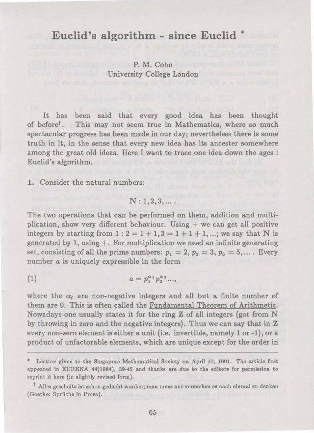
Euclid's algorithm - since Euclid *

P.M. Cohn University College London

It has been said that every good idea has been thought of beforet. This may not seem true in Mathematics, where so much spectacular progress has been made in our day; nevertheless there is some truth in it, in the sense that every new idea has its ancester somewhere among the great old ideas. Here I want to trace one idea down the ages : Euclid's algorithm.

1. Consider the natural numbers:

N: 1,2,3, ....

The two operations that can be performed on them, addition and multi­plication, show very different behaviour. Using + we can get all positive integers by starting from 1 : 2 = 1 + 1, 3 = 1 + 1 + 1, ... ;we say that N is generated by 1, using+. For multiplication we need an infinite generating set, consisting of all the prime numbers: p1 = 2, p2 = 3, p3 = 5, .... Every number a is uniquely expressible in the form

(1)

where the a, are non-negative integers and all but a finite number of them are 0. This is often called the Fundamental Theorem of Arithmetic. Nowadays one usually states it for the ring Z of all integers (got from N by throwing in zero and the negative integers). Thus we can say that in Z every non-zero element is either a unit (i.e. invertible, namely 1 or -1), or a product of unfactorable elements, which are unique except for the ord~r in

* Lecture given to the Singapore Mathematical Society on April 10, 1991. The article first appeared in EUREKA 44(1984), 39-45 and thanks are due to the editors for permission to reprint it here (in slightly revised form).

t Alles gescheite ist schon gedacht worden; man muss nur versuchen es noch einmal zu denken (Goethe: Spriiche in Prosa).

65

which they occur and for unit factors (e.g. 6 = 2·3 = ( -3)·( -2) etc.). This is expressed more briefly by saying: Z is a unique factorization domain, or more briefly still, a UFD.

In a UFD it is easy to describe the highest common factor (HCF) and least common multiple (LCM) of two members. Instead of (1) we can briefly write a= IIp;;. If b = IIp:; is another element, then we have

(2) (3)

HCF: (a, b)= II p:i,

LCM : [a, b] = II p~i,

where 6i = min{~,,Bi}, where J-ti = max{~,,Bd.

For example, take a = 36 = 22 • 32

, b = 50 = 2.52; then (a, b) = 2,

[a, b] = 900. If we know one of (2), (3), we can find the other by the formula : (a, b)[a, b] = ab, but this is of no help in finding the HCF and LCM themeselves, unless all factorizations (1) are known.

To find the HCF of two numbers a, b without factorizing them, Euclid [2] uses the division with remainder : if b > 0, there exist numbers q, r such that

(4) a= bq + r, 0 ~ r <b.

We now repeat the process with a, b replaced by b, rand continue in this way, getting a chain of equations

(5)

a= bq1 + r 1 ,

b = r 1 q2 + r 2 ,

r 1 = r2 q3 + r3 , b > r 1 > r2 > ...

r n- 1 = r n qn + 1 •

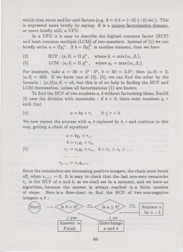
Since the remainders are decreasing positive integers, the chain must break off, when rn+ 1 = 0. It is easy to check that the last non-zero remainder rn is the HCF of a and b, as we shall see in a moment, and we have an algorithm, because the answer is always reached in a finite number of steps. Here is a flow-chart to find the HCF of two non-negative integers a, b :

Q ---+ ~ ~ ~ ~ Replace a 0 ~ ~ bya-b

lyes ~ lno Answer: a Interchange

Finish a and b

66

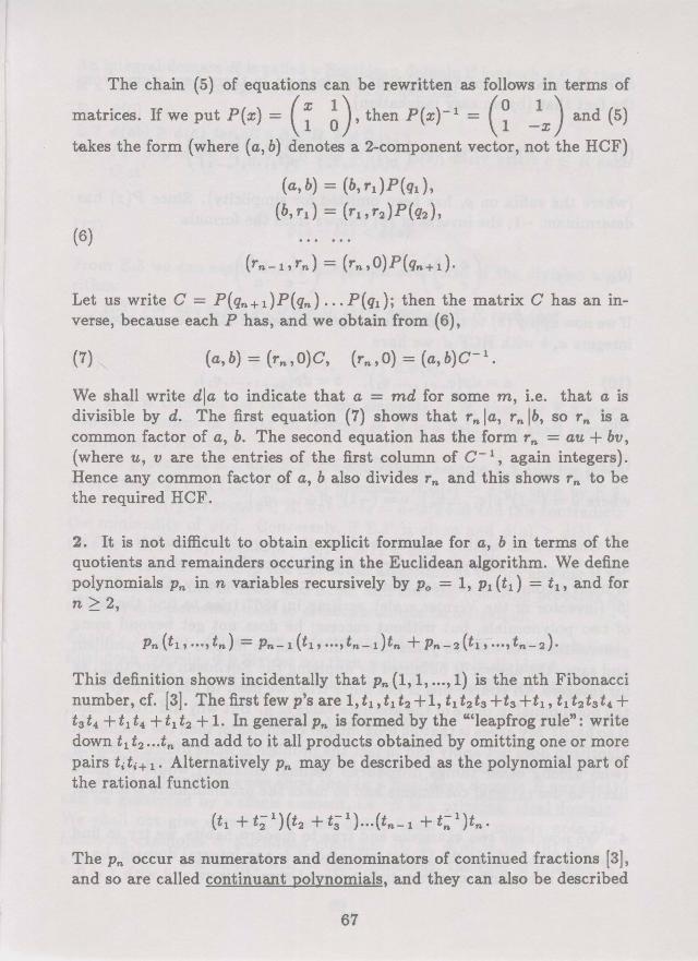
The chain (5) of equations can be rewritten as follows in terms of

. (X 1) (0 1 ) matnces. If we put P(x) = 1 0

, then P(x)- 1 = 1

-x and (5)

takes the form (where (a, b) denotes a 2-component vector, not the HCF)

(6)

(a, b) = (b, rt)P(qt),

(b,rt) = (r1,r2)P(q2),

Let us write C = P(qn+ t)P(qn) ... P(qt); then the matrix C has an in­verse, because each P has, and we obtain from (6),

(7) "

We shall write dia to indicate that a = md for some m, i.e. that a is divisible by d. The first equation (7) shows that r n Ia, r n lb, so r n is a common factor of a, b. The second equation has the form r n = au + bv, (where u, v are the entries of the first column of c- 1

, again integers). Hence any common factor of a, b also divides r n and this shows r n to be the required HCF.

2. It is not difficult to obtain explicit formulae for a, b in terms of the quotients and remainders occuring in the Euclidean algorithm. We define polynomials Pn in n variables recursively by Po = 1, p1 (t1) = t1, and for n 2:2,

This definition shows incidentally that Pn (1, 1, ... , 1) is the nth Fibonacci number, cf. [3]. The first few p's are 1, t1, t1 t2 + 1, t1 t2 t3 +t3 +t1, t1 t2 ts t, + t 3 t 4 +t1 t4 +t1 t2 + 1. In general Pn is formed by the "'leapfrog rule": write down t 1 t 2 ••• tn and add to it all products obtained by omitting one or more pairs t, ti+ 1 • Alternatively Pn may be described as the polynomial part of the rational function

The Pn occur as numerators and denominators of continued fractions [3], and so are called continuant polynomials, and they can also be described

67

as determinants (continuants), but our interest in them here stems from the fact that (by an easy inducation),

(8)

(where the suffix on p, has been omitted for simplicity). Since P(x) has determinant -1, the inverse of (8) follows from the formula

(9) (a b)- 1

=(-1)n ( d -b)· c d -c a

If we now apply (8) to the Euclidean algorithm we find that for any positive integers a, b with HCF d, we have

(10)

and

(11) d = bu- av,

3. One can ask similar questions about the ring of polynomials a0 xn + a 1 xn- 1 + ... +an with rational (or real) coefficients. The answer is now part of most second year courses, but it was not always so easy. Pedro Nunez [5] (inventor of the Vernier scale), writing in 1567 tries to find the HCF of two polynomials, but without success; he does not get beyond some generalities. Yet only 18 years later Simon Stevin [6] sets it as a problem and says: the answer is obtained by applying the Euclidean algorithm, as for integers. Of course this is not quite true, we need to use the degree of the polynomial in place of the absolute value of a. But why did Nuiiez find it so hard? My guess is that he took integer coefficients; then the Euclidean algorithm does not apply and in fact the problem is quite difficult. Stevin (who among other things introduced decimal notation) would be more likely to use rational coefficients and so make the problem more tractable.

4. We now have two examples and true to modern habits, we try to find a description to fit both. Our starting point is any integral domain, i.e. a ring (not necessarily commutative) without zero-divisors and with 1 =I= 0.

68

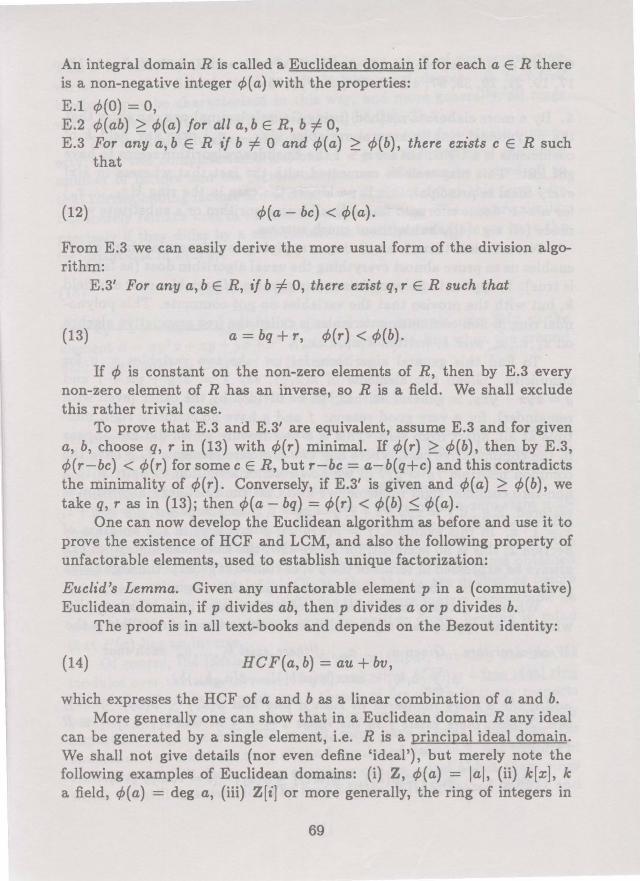
An integral domain R is called a Euclidean domain if for each a E R there is a non-negative integer 4>(a) with the properties:

E.1 4>(0) = 0, E.2 4>(ab) ~ 4>(a) for all a, bE R, b =/; 0, E.3 For any a, b E R if b =/; 0 and 4>(a) ~ 4>(b), there exists c E R such

that

(12) 4>(a- be) < 4>(a).

From E.3 we can easily derive the more usual form of the division algo­rithm:

E.3' For any a, b E R, if b =/; 0, there exist q, r E R such that

(13) a= bq + r, 4>(r) < 4>(b).

If 4> is constant on the non-zero elements of R, then by E.3 every non-zero element of R has an inverse, so R is a field. We shall exclude this rather trivial case.

To prove that E.3 and E.3' are equivalent, assume E.3 and for given a, b, choose q, r in (13) with 4>(r) minimal. If 4>(r) ~ 4>(b), then by E.3, 4>(r-bc) < 4>(r) for some c E R, but r-bc = a-b(q+c) and this contradicts the minimality of 4>(r). Conversely, if E.3' is given and 4>(a) ~ 4>(b), we take q, r as in (13); then 4>(a- bq) = 4>(r) < 4>(b) ~ 4>(a).

One can now develop the Euclidean algorithm as before and use it to prove the existence of HCF and LCM, and also the following property of unfactorable elements, used to establish unique factorization:

Euclid's Lemma. Given any unfactorable element p in a (commutative) Euclidean domain, if p divides ab, then p divides a or p divides b.

The proof is in all text-books and depends on the Bezout identity:

(14) HCF(a,b) =au+ bv,

which expresses the HCF of a and bas a linear combination of a and b. More generally one can show that in a Euclidean domain R any ideal

can be generated by a single element, i.e. R is a principal ideal domain. We shall not give details (nor even define 'ideal'), but merely note the following examples of Euclidean domains: (i) Z, 4>(a) = lal, (ii) k[x], k a field, 4>(a) = deg a, (iii) Z[i] or more generally, the ring of integers in

69

Q(Vd), <P(a) = lal, when d = -1, -2, -3, -7, -11 and 2, 3, 5, 6, 7, 11, 13, 17, 19, 21, 29, 33, 37, 41, 55, 73 (cf. [7],p.95).

5. By a more elaborate method (using Gauss's lemma) one can show that the polynomial ring in several variables k[x1, ... , Xn] over any field k of coefficients is a UFD, but for n > 1 the Euclidean algorithm seems to have got lost. This may well be connected with the fact that whereas in k[x] every ideal is principal, this is no longer the case in the ring k[x1 , ••• , Xn] for n > 1. Some efforts to find a Euclidean algorithm or a substitute were made (cf. e.g. [4]), but without much success.

Nevertheless there is an analogue applying to polynomial rings which enables us to prove almost everything the usual algorithm does (as far as it is true). It applies to polynomials in any number of variables over any field k, but with the proviso that the variables do not commute. This polyno­mial ring in non-commuting variables is called the free associative algebra on x1 , ••• , Xn over k, written k(x1 , ••• , Xn)·

To find this general algorithm, let us take two variables x, y for simplicity. Given two elements of k(x, y), say I = x 2 y + yx + 1 and g = xyx + yxy, in general neither can be divided by the other (even with remainder), for a very good reason: I and g have no common right mul­tiple at all, apart from zero. This is a new feature which did not appear in the commutative case, where any two non-zero elements I, g have the common multiple I g = gl. H we now restrict attention to pairs with a non-zero common right multiple, we find that the Euclidean algorithm is restored. E.g., if I= xyz+z+x, g = xy+ 1, then I= gz+x, g = x·y+ 1, x = 1 · x. In this example, I = p(x, y, z), g = p(x, y) in the notation of Section 2; this is no accident, for as we saw, the Euclidean algorithm can always be expressed in terms of the p's; of course in general the arguments of the p's will be much more complicated than this example.

What we actually need is a kind of n-term algorithm which applies whenever an appropriate right multiple condition is satisfied. This is the

Weak algorithm. Given a 1 , ••• ,am, af there exist b1 , ••• , bm such that

<P(La,bi) < max{<JI(a1 b!), ... ,<jl(ambm)},

and if the a's are numbered in such a way that <P( a1 ) ::; <P( a2 ) ::; ••• ::;

<P(am), then there exists i in the range 2::; i::; m and c1 , ••• ,c;_ 1 E R such that

j-1

<P(a;- l:a,c,) < <P(a;), <P(a.c,)::; <P(a;) (i = 1, ... ,;" -1). 1

70

This is satisfied by the free algebra k(X) in any set X of non-commuting variables over a field k, taking 4> to be the usual degree. In fact free algebras may be characterized in this way, and more generally, all rings with a week algorithm can be determined (cf. [1], Ch.2).

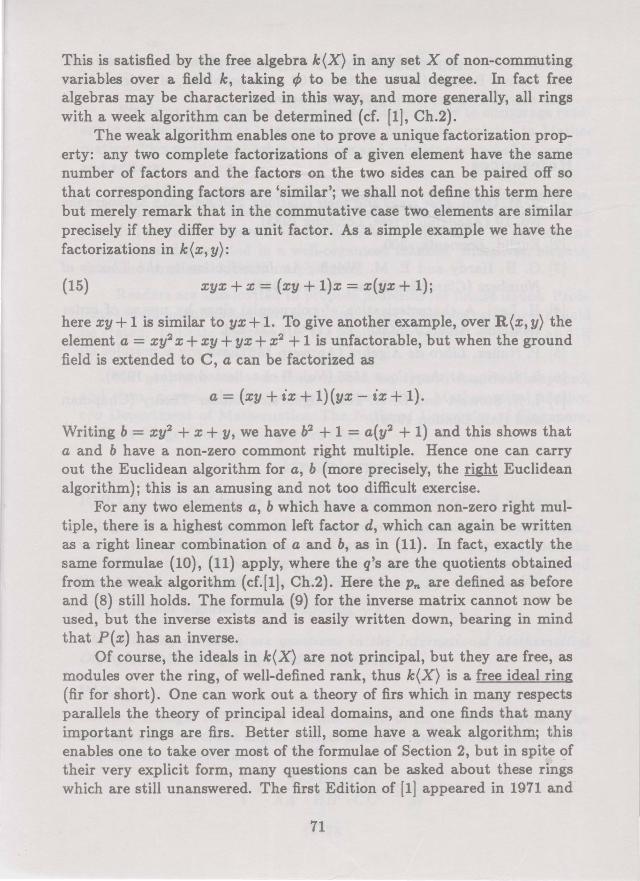
The weak algorithm enables one to prove a unique factorization prop­erty: any two complete factorizations of a given element have the same number of factors and the factors on the two sides can be paired off so that corresponding factors are 'similar'; we shall not define this term here but merely remark that in the commutative case two elements are similar precisely if they differ by a unit factor. As a simple example we have the factorizations in k(x, y):

(15) xyx + x = (xy + 1)x = x(yx + 1);

here xy + 1 is similar to yx + 1. To give another example, over R(x, y) the element a = xy2 x + xy + yx + x 2 + 1 is unfactorable, but when the ground field is extended to C, a can be factorized as

a= (xy + ix + 1)(yx- ix + 1).

Writing b = xy2 + x + y, we have b2 + 1 = a(y2 + 1) and this shows that a and b have a non-zero commont right multiple. Hence one can carry out the Euclidean algorithm for a, b (more precisely, the right Euclidean algorithm); this is an amusing and not too difficult exercise.

For any two elements a, b which have a common non-zero right mul­tiple, there is a highest common left factor d, which can again be written as a right linear combination of a and b, as in (11). In fact, exactly the same formulae (10), (11) apply, where the q's are the quotients obtained from the weak algorithm (cf.[1], Ch.2). Here the Pn are defined as before and (8) still holds. The formula (9) for the inverse matrix cannot now be used, but the inverse exists and is easily written down, bearing in mind that P(x) has an inverse.

Of course, the ideals in k(X) are not principal, but they are free, as modules over the ring, of well-defined rank, thus k(X) is a free ideal ring (fir for short). One can work out a theory of firs which in many respects parallels the theory of principal ideal domains, and one finds that many important rings are firs. Better still, some have a weak algorithm; this enables one to take over most of the formulae of Section 2, but in spite ()f their very explicit form, many questions can be asked about these rings which are still unanswered. The first Edition of [1] appeared in 1971 and

71

.. contained 86 open problems, of which 15 were solved)n the next 14 years. The Second Edition (1985) contains 103 open problems, of which 8 have been solved to date, leaving 95 still unsolved.

References

[1] P.M. Cohn, Free rings and their relations, 2nd Ed. LMS Monographs No. 19 (Academic Press, Londong 1985).

[2] Euclid, Elements, -300.

[3] G. H. Hardy and E. M. Wright, An Introduction to the Theory of Numbers (Clarendon Press, Oxford 1938).

[4] H. Levi, A characterization of polynomial rings by means of order relations, Amer. J. Math. 65 (1943), 221-234.

[5] P. Nunez, Libro de Algebra (Antwerp 1567).

[6] S. Stevin, Arithmetique 1585 (Vol. II of collected works, 1958).

[7] I. N. Stewart and D. 0. Tall, Algebraic Number Theory (Chapman and Hall, London 1979).

72