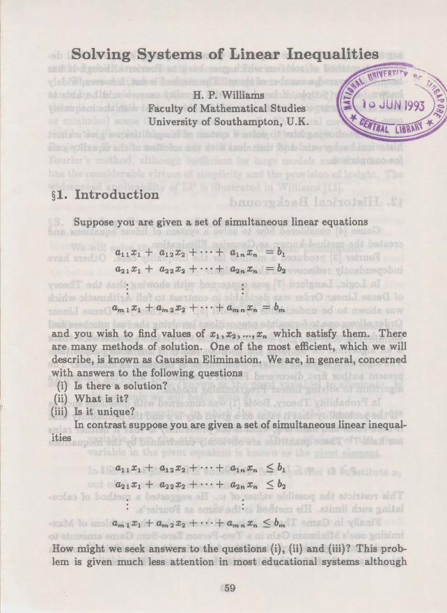
H. P. Williams Faculty of Mathematical Studies University of Southampton, U.K.

§l. Introduction

Suppose you are given a set of simultaneous linear equations

auxl + a12x2 + ... + alnXn = bl

~1X1 + ~2X2 + · · • + ~nXn = b2

and you wish to find values of x 1 , x2 , ••• , Xn which satisfy them. There are many methods of solution. One of the most efficient, which we will describe, is known as Gaussian Elimination. We are, in general, concerned with answers to the following questions

(i) Is there a solution? (ii) What is it?

(iii) Is it unique? In contrast suppose you are given a set of simultaneous linear inequal­

ities

auxl + a12x2 + ... + alnXn :$ bl

~1X1 + ~2X2 + • · · + ~nXn :$ b2

How might we seek answers to the questions (i), (ii) and (iii)? This prob­lem is given much less attention in most educational systems although

59

arguably it is even more important than the equality case. We will de­scribe a method of solution which goes back to Fourier although it has been rediscovered a number of times. The method is not, however, widely known. Many people, if faced with the equality case, would be able to solve it but, I suspect, not many would be able to deal with the inequality case.

Before showing how to solve a system of inequalities we give a short historical background and then deal with the solution of the equality case for comparison.

§2. Historical Background

Gauss [4] considered how to solve a system of linear equations and created the method known as Gaussian Elimination.

Fourier [3] produced a method for the inequality case. Others have independently rediscovered this method.

In Logic, Langford [7] was concerned with showing that the Theory of Dense Linear Order was decidable in contrast to full Arithmetic which was shown to be undecidable by Godel [5]. The Theory of Dense Linear Order allows one to formulate propositions involving the real numbers and an ordering relation "~". Such a theory is shown to be decidable if there is an algorithm for deciding the truth or falsity of any such proposition. The algorithm which he derived turns out to be the same as Fourier's. The present author first discovered Fourier's method by applying Langford's algorithm to solving Linear Programming models.

In Probability Theory, Boole [1] was concerned with questions such as "If the probability that it rains on a given day is p and the probability that it both rains and hails is q, what is the probability w that it neither rains nor hails ?" These quantities are obviously constrained by the inequalities

p ~ q, w ~ 1 - p, p ~ 0, q ~ 0, p ~ 1, q ~ 1.

This restricts the possible values of w. He suggested a method of calcu­lating such limits. His method is the same as Fourier's.

Finally in Game Theory, it is well known that the problem of Max­imising one's Minimum Gain in a Two-Person Zero-Sum Game amounts to choosing strategies with probabilities determined by inequalities. Motzkin [8] gave a method of doing this which is the same as Fourier's.

60

• I

Williams [10] gives a summary as well as a full description of the method which is now usually known as Fourier-Motzkin Elimination.

The need to solve linear inequality systems is now given great impor­tance by the widespread use of Linear Programming (LP) models. Here there is an added component in that one wishes to optimise (maximise or minimise) some linear expression as well. The usual method of solu­tion is the Simplex Algorithm due to Dantzig [2] although the method of Projective Transformations due to Karmarkar [6] is also sometimes used. Fourier's method, although inefficient for large models and little known, has the considerable virtues of simplicity and the provision of insight. The widespread applicability of LP is illustrated in Williams [11].

§3. Solving Systems of Linear Equations

We will solve the following system by Gaussian Elimination.

- Z1 + z~ - Zs = 2

Z1 + z~ + 2zs = 3

z~ + z3 = 3

Deliberately, we have given the same number of equations as variables and made sure that the matrix of coefficients is non-singular (has determinant #- 0). This guarantees that there is a unique solution.

Gaussian Elimination is performed by the following steps.

Step 1: Choose a variable (known as the pivot variable) to eliminate. In the example we will begin with z 1 •

Step 2: Choose an equation in which the pivot variable occurs and use this equation (known as the pivot equation) to eliminate the pivot variable from the other equations. The coefficient of the pivot variable in the pivot equation is known as the pivot element.

In this example we will choose the first equation to substitute z 1

out of the other equations and give

2z~ + Zs = 5

z~ + Zs = 3.

Note that this step can be performed by adding or subtracting suitable multiples of the pivot equation from the other equations.

61

Steps 1 and 2 are repeated to eliminate x2 and give

1 1 - Xs =-. 2 2

Step 3: We back substitute to obtain

x3 = 1

x2 = 2

xl = -1.

There is flexibility in which elements we choose as pivot elements and in what order. This does not concern us but is very important in practice.

For a general problem we consider how the method would cope with questions (i), (ii) and (iii).

H the last elimination had also happened to remove the last variable x3 we could have ended up with a contradiction such as 0 = 1. This would have indicated that there were no solutions.

H either at the end, or at some intermediate stage, we had ended up with a non-contradictory but valid equation such as 0 = 0 this would have enabled us to set the variable (eg. x3 ) ·to any value showing that there are more than one solution.

Our example clearly indicates case (iii) where there is a unique solu­tion.

§4.. Solving Systems of Linear Inequalities

We will solve the following system by the method of Fourier.

4xl - Sx2 - 3xs + z :5 0 cO

-x1+ x2- Xs :52 c1

x1 + X2 + 2xs :53 c2

-xl :50 c3

x2 :50 c4

Xs :50 c5

Readers familiar with Linear Programming will recognize why I have cre­ated an example in this form. I have delibrately made the variables non­negative and introduced an extra variable z to represent an objective func­tion. This is not, however, necessary for our general method. If we had

62

simply taken an inequality version of our equality system, the solution would have been rather trivial.

We will perform the following steps.

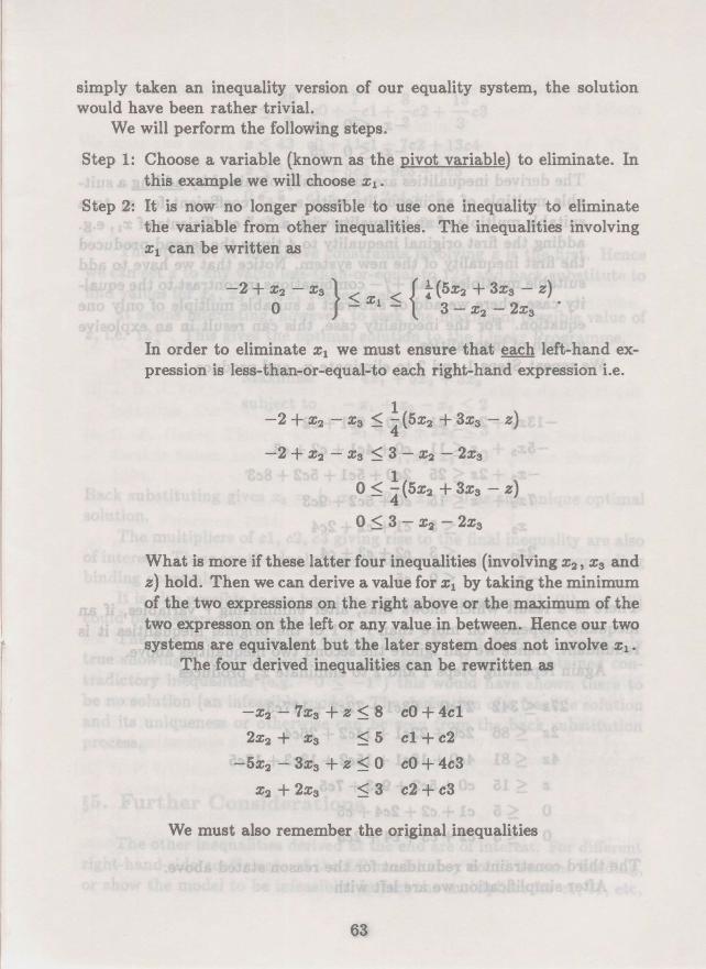
Step 1: Choose a variable (known as the pivot variable) to eliminate. In this example we will choose x1 •

Step 2: It is now no longer possible to use one inequality to eliminate the variable from other inequalities. The inequalities involving x1 can be written as

In order to eliminate x1 we must ensure that each left-hand ex­pression is less-than-or-equal-to each right-hand expression i.e.

1 -2 + x2 - Xs ~ 4 ( 5x2 + 3x8 - z)

-2 + X2 - Xs ~ 3 - X2 - 2xs 1

0 ~ 4(Sx2 + 3x8 - z)

0 ~ 3- x2 - 2xs

What is more if these latter four inequalities (involving x2 , x8 and z) hold. Then we can derive a value for x1 by taking the minimum of the two expressions on the right above or the maximum of the two expresson on the left or any value in between. Hence our two systems are equivalent but the later system does not involve x1 •

The four derived inequalities can be rewritten as

-x2- 7x8 + z ~ 8 cO+ 4c1

2x2 + Xs ~5 c1 +c2

-5x2 - 3x8 + z ~ 0 cO+ 4c3

X2 + 2xs ~3 c2 +c3

We must also remember the original inequalities

63

-x2 :50 c4

-xs :50 c5

The derived inequalities are more easily obtained by adding a suit­able multiple of an inequality with a "+" coefficient for x1 to a suitable multiple of an inequality with a "-" coefficients of x1 , e.g. adding the first original inequality to 4 times the second produced the first inequality of the new system. Notice that we have to add suitable multiples of all + /- combinations in contrast to the equal­ity case where we add or subtract a suitable multiple of only one equation. For the inequality case, this can result in an explosive growth of inequalities.

We repeat Steps 1 and 2 to eliminate x2 and produce

-13x3 + 2z :5 21 2c0+ 9c1 + c2

-5x3 + z :5 11 cO + 4c1 + c2 + c3

-Xs + 2z :5 25 2c0 + 5c1 + 5c2 + 8c3

7xs + z :5 15 cO+ 5c2 + 9c3

Xs :55 c1 + c2 + 2c4

2xs :53 c2 + c3 + c4

-Xs :50 c5

There is a result which shows that, after eliminating r variables, if an inequality depends on more than r + 1 of the original inequalities it is redundant. Hence we can ignore the second two inequalities above.

Again repeating Steps 1 and 2 to eliminate x3 produces

27z :5 342 27c0 + 63c1 + 72c2 + 117c3

2z :5 86 2c0 + 22c1 + 14c2 + 26c4

4z :5 81 4c0 + 18c1 + 15c2 + 13c3 + 13c5

z $ 15 cO + 5c2 + 9c3 + 7 c5

0 < 5 c1 + c2 + 2c4 + c5

0 :5 3 c2 + c3 + c4 + 2c5

The third constraint is redundant for the reason stated above. After simplification we are left with

64

38 7 8 13 z ~ a cO+ 3c1 + 3c2 + 3 c3

z ~ 43 cO+ llc1 + 7c2 + 13c4

z ~ 15 cO + 5c2 + 9c3 + 7 c5

0 ~ 5 c1 + c2 + 2c4 + c5

0 ~ 3 c2 + c3 + c4 + 2c5

The strictest of the above constraints involving z is the first. Hence we can set z to any value less-than-or-equal-to 12~ and back substitute to find values for x3 , x2 and x1 respectively.

It seems interesting, however, to seek the maximum possible value of z, 1.e. 12~ . This gives the optimal solution to the Linear Programme.

Maximise

subject to

- 4x1 + 5x2 + 3x3

- X1 + X2 - Xs ~ 2

x1 + X2 + 2xs ~ 3

x1,x2 , x3 ~ 0

Back substituting gives x3 = ~' x2 = 2~, x1 = 0 as the unique optimal solution.

The multipliers of c1, c2, c3 giving rise to the final inequality are also of interest. These are the dual values (shadow prices) on the corresponding binding constraints.

It is also possible to see how the answers to questions {i), (ii) and (iii) could be answered in general.

The final two inequalities derived ("0 ~ 5" and "0 ~ 3") are clearly true showing a feasible solution to be possible. H we had obtained con­tradictory inequalities (e.g. "0 ~ -1") this would have shown there to be no solution (an infeasible model). The derivation of a feasible solution and its uniqueness or otherwise can be seen from the back substitution process.

§5. Further Considerations

The other inequalities derived at the end are of interest. For different right-hand-side coefficients of the LP model they could become binding, or show the model to be infeasible. In fact the multipliers for cO, c1, etc,

65

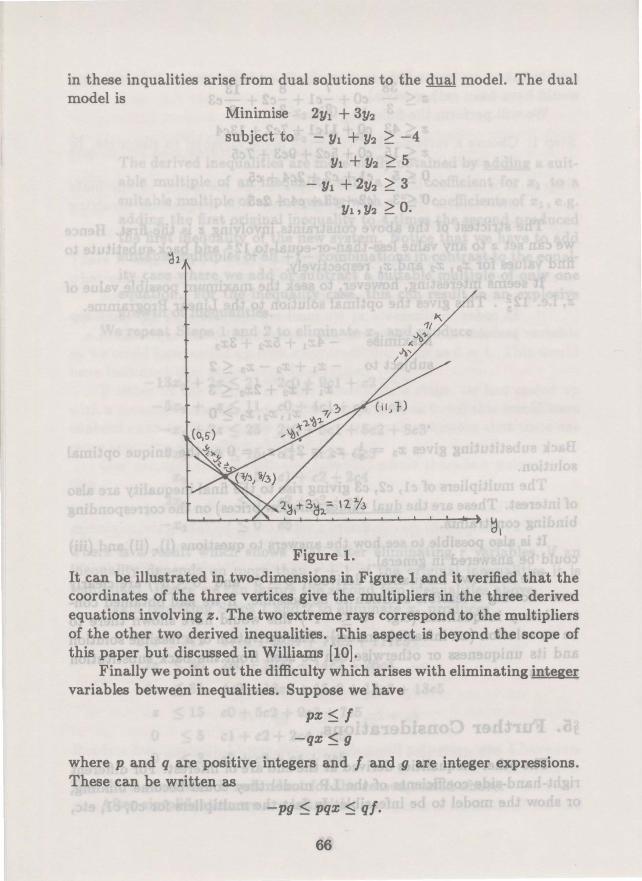
in these inqualities arise from dual solutions to the dual model. The dual model is

Minimise 2yl + 3y2

subject to - Y1 + Y2 ~ -4

Y1 + Y2 ~ 5

- Y1 + 2y2 ~ 3

Y1,Y2 ~ 0.

Figure 1.

It can be illustrated in two-dimensions in Figure 1 and it verified that the coordinates of the three vertices give the multipliers in the three derived equations involving z. The two extreme rays correspond to the multipliers of the other two derived inequalities. This aspect is beyond the scope of this paper but discussed in Williams [10].

Finally we point out the difficulty which arises with eliminating integer variables between inequalities. Suppose we have

pz ~I

-qz ~ g

where p and q are positive integers and I and g are integer expressions. These can be written as

-pg ~ pqz ~ ql.

66

It is not sufficient to produce

-pg ~ qf.

We must also assert that a multiple of pq lies between -pg and qf. This is more complicated and involves the use of linear congruences and the Chinese Remainder Theorem. It is discussed by Williams [9] and [12].

References

[1] G. Boole, On the conditions by which the solutions of questions in the theory of probabilities are limited, The Philosophical Magazine, Series 4, Vol. viii, 1854.

[2] G. B. Dantzig, Linear Programming and its extensions, Princeton, 1963

[3] J. B. J. Fourier, Solutions d'une question particuliere du calcul des inegalites, Oeuvres II, Paris 1826, 317-328.

[4] C. F. Gauss, Theoria Motus Corporum Coolestium in Sectionitus Conicis Solem Ambientium, F. Perthes and J. H. Bessor Hombury, 1804.

[5] K. Godel, On Undecidable Propositions of Formal Mathematical Sys­tems, Princeton, 1934.

[6] N. Karmarkov, A New Polynomial-Time Algorithm for Linear Pro­gramming, Proceedings of the 16th Annual ACM Symposium of the Theory of Computing, Washington, DC, April 30-May 2, 1984, 302-310.

[7] C. H. Longford, Some Theorems on Deducibility, Ann. of Math., I, 28, 1927' 16-40.

[8] T. S. Motzkin, Beitrage zur Theorie der Linearm Ungleichungen, Dis­sertation, University of Basel, Jerusalem, 1936.

[9] H. P. Williams, Fourier-Motzkin Elimination Extension to Integer Programming, J. Combinatorial Theory, Series A, 21, 1976, 118-123.

[10] H. P. Wil~iams, Fourier's Method of Linear Programming and its Dual, American Math. Monthly, 93, 1986, 681-695.

[11] H. P. Williams, Model Building in Mathematical Programming, 3rd Edition, Wiley 1990.

[12] H. P. Williams, The Elimination of Integer Variables, Journal of the Operational Research Society, to appear, 1992.

67