EU Enlargement and Technology Transfer to New Member States

EU Enlargement andTechnology Transfer to New Member States

Simla Tokgoz

Working Paper 05-WP 414November 2005

Center for Agricultural and Rural DevelopmentIowa State University

Ames, Iowa 50011-1070www.card.iastate.edu

Simla Tokgoz is an associate scientist at the Center for Agricultural and Rural Development and aninternational grain analyst with the Food and Agricultural Policy Research Institute, Iowa State University.

This paper is available online on the CARD Web site: www.card.iastate.edu. Permission is granted toreproduce this information with appropriate attribution to the author.

Questions or comments about the contents of this paper should be directed to Simla Tokgoz, 560BHeady Hall, Iowa State University, Ames, IA 50011-1070; Ph: (515) 294-6357; Fax: (515) 294-6336;E-mail: [email protected]

Iowa State University does not discriminate on the basis of race, color, age, religion, national origin, sexual orientation, genderidentity, sex, marital status, disability, or status as a U.S. veteran. Inquiries can be directed to the Director of Equal Opportunity andDiversity, 3680 Beardshear Hall, (515) 294-7612.

Abstract

The European Union (EU) accomplished its biggest enlargement process in 2004 in terms of

the number of countries, area, and population. This study focuses on the impact of enlargement,

the resulting technology transfer on the grain sectors of the New Member States (NMS), and the

consequent welfare implications. The study finds that EU enlargement has important

implications for the EU and the NMS, but its impact on the world grain markets is minimal. The

results show that producers in the NMS gain from accession because of higher prices, whereas

consumers in most NMS face a welfare loss. Incorporating technology transfer into the accession

increases the welfare gain of producers despite falling prices because of the larger supply shift.

The loss of welfare for consumers in most NMS is lower in this case because of the decline in

grain prices.

Keywords: EU enlargement, technology transfer, welfare.

JEL: F15, Q17, D6

1

EU Enlargement and Technology Transfer to New Member States

Introduction

At the end of 2003, the European Union (EU) concluded its negotiations with 10

candidate countries,1 and in 2004 it accomplished its largest enlargement process in terms of the

number of countries, area, and population. This development is significant for world grain

markets, as the EU has been a large importer and exporter. Moreover, the enlargement will have

some substantial impacts within the EU because the agricultural sector is critically important in

the New Member States (NMS).

The agricultural sector of the NMS generates a higher percentage of the GDP and

employs a larger portion of the labor force relative to the EU-15. However, the structural

inefficiency of the farms, a residual consequence of collectivization after World War II, has lead

to low agricultural output levels in these countries, which were once considered the “bread

basket” of Europe. Financial and capital constraints contributed to lower yields, as they limited

the purchase of inputs by farmers. Although the yield levels have started converging toward the

EU-15 levels in recent years, there is still much potential to be realized in the NMS.

Many instruments of the common agricultural policy (CAP) of the EU, such as direct

payments to farmers, are expected to benefit the agricultural producers of the NMS and increase

their production and export levels. With their accession to the EU, not only will agricultural and

trade policies of the NMS be harmonized with the EU but the NMS also will benefit from

technology transfer from the EU-15 members through foreign direct investment (FDI).

Bevan and Estrin (2004) analyze the determinants of FDI from Western countries,

particularly in the EU, to Central and Eastern European Countries (CEEC). They show that

2

announcements about EU accession proposals increase the levels of FDI to the prospective

members. Sinani and Meyer (2004) focus on the role of FDI in generating technology spillovers

to host economies in the case of Estonia. Their study demonstrates the positive effect of

technology transfer on the productivity of domestic manufacturing firms in Estonia.

Technology transfer will also affect the supply response in the agricultural sectors of the

NMS after the enlargement, as well as the CAP. Thus, the impact of technology transfer and the

supply response it generates in the NMS need to be considered when evaluating the impact of

EU enlargement on the NMS, EU, and world grain markets.

In this respect, this study analyzes the impact of the EU enlargement on the NMS, EU-15,

and world grain markets as well as the impact of technology transfer on the grain sectors of the

NMS after the accession. The main objective is to compute the changes in welfare in the NMS

because of the accession and the resulting technology transfer. Enlargement creates three

different shocks to the grain sectors of the NMS: change in tariff rates in the NMS, phasing in of

CAP instruments, and technology transfer. As the potential technology transfer in the grain

sector of the NMS is well documented, as will be discussed in a later section, this study focuses

on the grain sector.

In this context, I first set up a benchmark scenario in which the EU has adopted CAP

reforms of 2003 but EU enlargement has not taken place. In the first scenario, only the trade

policy of the NMS is harmonized with the EU-15; thus, tariff rates in the NMS are adjusted to

their levels in the EU-15. In the second scenario, all the changes in the agricultural and trade

policies from accession are implemented in the grain sector of the NMS. In the third scenario,

technology transfer is added to accession, where the grain yields in the NMS converge to the

3

average yield level in the EU-15. The net welfare changes in each scenario are calculated and

compared.

To compute the net change in welfare, the change in tariff revenue, the change in

producer surplus, the change in consumer welfare, and the change in the export subsidy

expenditures are calculated for the NMS. The net change in welfare for the NMS can be either

positive or negative, depending on the direction and the relative magnitudes of these changes.

Before the EU enlargement took place, there were many studies in the literature on the

possible impacts of enlargement. However, these studies were based on conjectures on which

countries would join, as well as the terms of the future agreements. Two new studies that

incorporate the latest decisions of the Copenhagen agreement are discussed below.

Previously, Jensen and Frandsen (2003) analyzed the economic implications of the

Copenhagen accession agreement for EU member states with a global general equilibrium model

for the agricultural sector. The authors include welfare impacts of the accession and the

budgetary costs for pre- and post-enlargement scenarios. They find enlargement to be primarily

an intra-European event with minor impacts on countries outside Europe. However, this study

does not incorporate the CAP reform of 2003, and it is based on Agenda 2000. Fabiosa et al.

(2005) assess the impacts of EU enlargement and the CAP reform of 2003 separately. Their

study focuses on international dairy, grains, livestock, oilseeds, and sugar markets. However, it

does not provide any welfare analysis or a technology transfer scenario.

The model used in the present study includes the CAP reform of 2003 and the latest

decisions on the phasing in of the CAP in the NMS. The analysis includes three different

scenarios that decompose the different phases of the accession and its impact on the world grain

markets. The third scenario adds a technology transfer scenario to the enlargement, as it is a

4

crucial outcome of the enlargement. It includes welfare analysis for the NMS in each scenario,

thus distinguishing the different impacts of policy changes and technology transfer on welfare in

the NMS.

The study finds that EU enlargement has important implications for the EU and the NMS,

but its impact on world grain markets is minimal. However, adding technology transfer to the

accession scenario results in much bigger impacts on world markets, particularly on grain prices.

Producers in the NMS gain from the accession because they benefit from higher prices, while

consumers face a net welfare loss in most of the NMS. Incorporating technology transfer into the

accession increases the welfare gain of producers despite falling prices, as the supply shift is

much larger in this scenario. The loss of welfare for consumers in most of the NMS is lower in

this scenario because of the slight decline in grain prices brought about by the larger supply

response.

The literature on immiserizing growth is helpful to an analysis of welfare effects of a

technology transfer in the NMS. Bhagwati (1958) reintroduced the concept of immiserizing

growth, i.e., that technical progress may reduce social welfare through adverse effects on the

terms of trade in an economy. Johnson (1967) showed that growth could be immiserizing

because of trade policy distortions even when the terms of trade do not change. Alston and

Martin (1995) showed how the size and the distribution of benefits from research-induced supply

shift depending on the nature of the supply shift, the nature of any market-distorting policies, and

the terms-of-trade effects arising from technology transfer.

This study also explores the possibility of immiserizing growth in the grain sectors of the

NMS after their accession to the EU. The calculation of welfare changes in the third scenario

shows that this is not the case. In the third scenario, lower prices generated by the supply shift

5

were not large enough to create a negative change in producer surplus in the NMS. Although the

export subsidy expenditures in the third scenario were much higher than in the second scenario,

they were not high enough to generate a negative welfare change and lead to immiserizing

growth.

The study proceeds as follows. The first section presents the general structure of the

international grain model. This is followed by a description of the grain model for the NMS. The

formulae used for welfare computations in each scenario are presented. Then, the three scenarios

included in the study are described. The impact of technology transfer in grain markets and the

different channels through which technology transfer in the NMS can take place are discussed

next. The last two sections give the corresponding results and conclusions.

An International Grain Model

We start with the FAPRI International Grain Model, which is a non-spatial multi-market

model composed of 40 countries and regions, including a rest-of-the world aggregate, but this

model is augmented to incorporate technology transfer and computation of welfare changes in

the NMS. The data sources included in the model are the Production, Supply and Distribution

data set from the Foreign Agricultural Service of the U.S. Department of Agriculture, the

International Financial Statistics historical macroeconomic data from the International Monetary

Fund, and Global Insight’s macro forecast for the outlook portion of the model. Necessary

commodity prices and policy information come from U.S. Foreign Agricultural Service Attaché

Reports, the World Trade Organization, publications of the Economic Research Service of the

U.S. Department of Agriculture, EU Commission publications, and the CAP Monitor.

The commodities included in the model are barley, corn, sorghum, and wheat. Each

country sub-model consists of at least one commodity depending on the relative importance of

6

the commodity and the relative importance of the country in the world markets as a supplier or a

buyer. In terms of the structure of the models, the following identity is satisfied for each country,

region, and the world: {Beginning stock + Production + Imports} = {Ending Stock +

Consumption + Exports}. The detailed description of the model, agricultural and trade policy

assumptions, and the major elasticities used in the model are provided on the FAPRI Web site

(http://www.fapri.iastate.edu). Parameters in the model such as price and income responses are

directly estimated, surveyed from the literature, or obtained from consensus of expert opinions

(FAPRI 2005).

Production is divided into yield and area equations, while consumption is divided into

feed and non-feed demand. In the EU model, a domestic price is solved for barley, corn, and

wheat that will satisfy the above identity for all members of the EU-15 and NMS.

Agricultural and trade policies in each country are included in the model to the extent that

they affect the supply and demand decisions of the economic agents. Taxes on exports and

imports, tariffs, tariff rate quotas, export subsidies, intervention prices, and set aside rates in the

EU are a few examples of the policies integrated into the model.

The grain model assumes that the existing agricultural and trade policy variables will

remain unchanged in the outlook period. Macroeconomic variables, such as GDP, population,

and exchange rates, are exogenous variables that drive the projections of the model.

A Grain Model for the NMS

For the Czech Republic, Hungary, and Poland, separate models are set up for barley,

corn, and wheat. Cyprus, Estonia, Latvia, Lithuania, Malta, Slovakia, and Slovenia are grouped

together under the name “Other NMS.” The sub-model for each country includes behavioral

equations for area harvested, yield, production, and beginning stocks on the supply side, per

7

capita consumption, feed demand per grain consuming animal unit (GCAU), and ending stocks

for the demand side. Net trade is a residual that equates supply and demand.

Below is the description of a generic model for each country, using corn as an example.

The equation for area harvested for corn is written as

( , )C C B C B C C B BA A P y P y (1)

where CP is the price of corn in real terms, Cy is the yield for corn, and BP and By denote the

real price and yield of the substitute crops respectively.

The production per hectare (yield) is set up as

* C CC

y P TrendP

(2)

where a trend is included to capture the rate of technical change prior to the accession.

Combining equations (1) and (2), the corn production equation is derived as

( ) ( )C C C B B CS P y P y P Trend (3)

Corn consumption per capita is determined by real price of corn, real price of substitute

crops, and income per capita as

( , , )C C BD f P P I (4)

where I denotes per capita GDP.

Feed demand per GCAU is determined by lagged feed demand, real price of corn, and real

price of substitute crops as

, 1( , , )C C t C BG f G P P (5)

Ending stocks are determined by lagged ending stocks and real price of corn as

, 1( , )C C t CES f ES P (6)

8

Measuring Welfare Changes

To calculate welfare changes, first a benchmark is established. Then, each scenario is

evaluated relative to this benchmark using change in tariff revenue (TR), producer surplus (PS),

equivalent variation (EV), and export subsidy expenditure (ES).2

Change in Tariff Revenue

Change in tariff revenue is written as

Tariff Revenue=(New Flow*New Tariff Rate*New Price)-(Old Flow*Old Tariff Rate*Old Price) (7)

Producer Surplus

The formula used for computation of the producer surplus is

ˆ)( dxxLPS x (8)

where ̂represents the profits in each scenario and represents the benchmark profits. xL is

the land allocated to the specific commodity.

Consumer Welfare

Equivalent variation (EV) is used to measure the change in consumer welfare. An

incomplete demand system approach (LINQUAD) is used as it allows an exact welfare measure

to be derived from it (LaFrance 1998; LaFrance et al. 2002; and Agnew 1998).

First, a representative consumer with an expenditure function ),( UPfe is assumed,

where P is a vector of consumer prices, ),,( OGBC PPPP , and U denotes utility. In the example

below, the focus is on a two-good case of the utility function that includes corn and barley. Each

country has a different consumption equation for each commodity, and the EV calculation has

been adjusted for each different case. CP denotes the price of corn, BP denotes the price of

9

barley, OGP refers to the price of all other goods that are included for completeness, and

M denotes income.

The Marshallian demands for corn and barley, denoted by CD and BD respectively, are

derived as follows:

)5.05.0(),,( 22BBCCBBCCCCCCBCC PPPPMxPMPPD (9)

and

)5.05.0(),,( 22BBCCBBCCBBBBBCB PPPPMxPMPPD (10)

for all countries.

In the next step, the following system of equations is solved with the above two equations

to obtain the parameters CCCBBB xx ,,,,, :

BBBBBB

B PxPD

(11)

BB x

MD

(12)

CCCCCC

C PxPD

(13)

CC x

MD

(14)

The solution allows exact identification of all cross-price responses to the system, as ,

and x are then known parameters. Based on equations (9) and (10), the EV is derived as

0011212111 exp)(5.0)(5.0 BBCCBBCCBBCCBBCC PxPxPxPxPPPPMEV

202000 )(5.0)(5.0 BBCCBBCC PPPPM (15)

where 0 and 1 denote the initial and the final prices, respectively.

10

Export Subsidy

An effective export subsidy rate is calculated for each commodity for the EU-15 by using

the latest available value of export subsidy expenditure and the FOB values of exports for that

year.

Per unit export subsidy rate = )(EX

ER (16)

where ER denotes the value of export refunds (export subsidy expenditures), and EX represents

the value of exports (FOB price times total exports). This subsidy rate is used for each NMS to

calculate its export subsidy expenditures and the changes after each scenario. Thus, the total

export subsidy expenditure gets evenly distributed with respect to the export shares of each

country for each commodity. The export subsidy expenditure for each country and commodity is

calculated by multiplying the export subsidy rate by the FOB price of the commodity and the

third-country3 exports.

The subsidy rate for each commodity in the EU is calculated based on the latest available

data. This subsidy rate is used across all the acceding countries to be consistent, which resulted

in an even distribution of export subsidies to acceding countries with respect to their export

shares. However, some of the acceding countries had export subsidies prior to the enlargement,

and ambiguity about their future utilization has prompted the above methodology. Thus, the

utilization of export subsidies by the NMS after joining the EU may differ from the one

described in this study.

The net change in welfare is computed as

Welfare TR PS EV ES (17)

11

Scenarios

First, a benchmark scenario (baseline) is set up that includes the CAP reform of 2003 in

the EU without accession. This is necessary in order to be able to trace the impact of policy

changes and technology transfer on grain sectors of the candidate countries and the resulting

welfare changes.

In Scenario 1, only the changes in the tariff rates for barley, corn, and wheat in the NMS

are incorporated into the model. The pre-accession and post-accession tariff rates for the Czech

Republic, Hungary, Other NMS, and Poland are given below in Table 1.

Table 1. Tariff rates in the New Member States (10-year average)Czech Republic

(percent)Hungary(percent)

Other NMS(percent)

Poland(percent)

WheatPre-accession 21.20 32.00 31.76 22.50Post-accession 10.43 10.43 10.43 10.43CornPre-accession 17.00 32.00 14.33 20.00Post-accession 25.67 25.67 25.67 25.67BarleyPre-accession 21.20 32.80 33.04 20.00Post-accession 14.64 14.64 14.64 14.64Note: Other NMS includes Cyprus, Estonia, Latvia, Lithuania, Malta, Slovakia, and Slovenia.Their tariff rates are an average of each individual country tariff rate weighted by production.

Scenario 2 includes full accession of the 10 NMS in May 2004. NMS adopt the CAP but

with certain changes in the policy variables that allow them to phase in the changes. The policy

changes are given in Table 2 and Table 3. A major instrument of the CAP is arable area

payments to farmers. EU-15 will provide a portion of these payments, whereas the NMS can

provide up to 30% of these payments through different resources. The Single Farm Payment will

be a part of CAP for the NMS at the time of entry; thus, the decoupling rate is set to 100% in the

model for the NMS. Set-aside starts in 2009 at 10% and remains the same throughout the rest of

12

the projection period. Some of the NMS had export subsidy policies prior to accession. With the

enlargement, all of the NMS will become part of the EU export subsidy policy. The upper limit

for EU-25 for the wheat export subsidy is 14.4 million metric tons and 1.3 billion euros. For

coarse grain export subsidies, this upper limit is 10.8 million metric tons and 1.0 billion euros.

Scenario 3 incorporates technology transfer to the NMS as well as the full accession. The

technology transfer scenario is based on the idea of NMS agricultural sectors “catching up” with

the agricultural sectors of the EU countries. The average level of yields in the EU-15 and the

respective yields in the NMS are compared as a first step. The main rationale is that the yields in

the EU-15 reflect the potential for the yield levels in the NMS. In other words, EU-15 yield

levels represent a frontier for the yields in the NMS.

Table 2. EU payments and top-up payments in the New Member StatesPayments 2004 2005 2006 2007 2008 2009 2010 2011 2012 2013

(Percent)

Top-up 30 30 30 30 30 30 30 30 30 30

EU payments 25 30 35 40 50 60 70 70 70 70

Total 55 60 65 70 80 90 100 100 100 100

Table 3. Summary of CAP instruments in the New Member StatesPolicy 2004 2005 2006 2007 2008 2009Decoupling Rate (percent) 100 100 100 100 100 100

Set-aside (percent)* 0 0 0 0 0 10

Durum aid (euro/mt) 313.0 291.0 285.0 285.0 285.0 285.0

Intervention price (euro/mt) 101.3 101.3 101.3 101.3 101.3 101.3

Arable Area Payment (euro/mt) 63.0 63.0 63.0 63.0 63.0 63.0

* Average set-aside prior to exemption for small producers

13

The next question in this context is how long it takes for the NMS to catch up. That is a

difficult thing to predict, as it depends on the relative magnitude of the flow of FDI and the

structure of farms in the NMS. In the first phase of the accession, the NMS will benefit from an

initial flow of knowledge and capital from the EU member states. In the later stages, this flow of

knowledge and capital will continue to aid restructuring of the farms and renewal of the

production technology. Thus, in Scenario 3, the yield levels in the NMS increase in the first year

of the accession and later start converging toward the average EU-15 level. How much should

they converge to the EU-15 level? The projections are carried out 10 years ahead until the

2013/14 marketing year. Ten years will not be enough for all the NMS to catch up with the EU,

given the gap between their yields. Thus, it is assumed that nearly 50% of the gap between yield

levels will be reduced through technology transfer. The original yield levels in Scenario 2 and

the new yield levels in Scenario 3 are given in Appendix Tables A.1 through A.3, along with the

average EU-15 levels for each crop.

It should also be noted that the soil conditions and the climate impact the yield levels as

much as the input levels and technology. Some candidate countries are located in different agro-

ecological zones so their potential for yield growth may be different from each other. Therefore,

choosing a technology transfer scenario in which the gap between the respective yields are

narrowed rather than choosing a constant rate of yield growth allows the model to capture the

different potentials for each crop in each country.

Impact of Technology Transfer in Grain Markets

Figure 1 shows the impact of technology transfer in the grain markets of the NMS. Panel

(a) represents the domestic market and panel (b) represents the export market. This figure shows

the case for a large country exporter with an export subsidy policy in place.

14

Figure 1. Effects of technology transfer on production, prices, and exports of grains in the NMS

In panel (a), point A denotes the autarky equilibrium. Point B represents the autarky

equilibrium when the supply curve shifts in the NMS because of technical change after accession

to the EU. The domestic price denoted by PD0 decreases to PD

1 with the increased supply. A

pivotal shift of the supply curve is shown in Figure 1, where Supply (S0) shifts to S1. A parallel

shift or a combination of a pivotal and parallel shift is possible as well.

The export market is represented in panel (b) of Figure 1, where ED denotes excess

demand without the export subsidy and EDS denotes excess demand with the export subsidy. The

rectangle (PD0ECPW

0) represents the amount of export subsidy used before the supply shift. PW0

denotes the world price before the supply shift. In the export market, the excess supply (ES0)

shifts to ES1 after the technology transfer, changing the export subsidy amount to the rectangle

shown by (PD1FDPW

1). Although the supply shift in the domestic market is pivotal, the supply

shift in the export market is nearly parallel.

N

PD1

PD0 PD

0

S1

DD

S0

J

M

PricePrice

Quantity QuantityQ0 Q1 QE

0 QE1

(a) Domestic Market (b) Export Market

ES0

ES1

ED

PD1

PW0

PW1

C1C0

L

E

F

C

D

A

B

K

EDS

15

The welfare changes in the NMS from the technology transfer can be summarized as

follows. The change in consumer surplus is equal to the area denoted by (PD0JLPD

1), which is

positive. The change in producer surplus is equal to the difference in the areas, i.e., (PD1MN)–

(PD0KN), which can be either positive or negative. The increase in export subsidy expenditure is

equal to the area (CDFE), which is positive. The net welfare change is equal to the change in

consumer surplus plus the change in producer surplus minus the change in export subsidy. This

net change in welfare can be positive or negative, depending on the relative magnitude of its

components. If it is negative, then immiserizing growth occurs, i.e., the country is worse off after

a supply increase due to technical change. If it is positive, then the country benefits from the

technical change.

It is crucial to note that the nature of the supply shift and the size and nature of the trade

distortion will determine whether there will be immiserizing growth or not. Alston and Martin

(1995) discuss a set of conditions under which technological change can be immiserizing. Panel

(a) illustrates a pivotal supply shift. In this case, there is a possibility of immiserizing growth

even without trade distortion, as the change in producer surplus can be either positive or

negative. If the supply shift had been parallel, then producers would have benefited alongside

consumers, unless there is a trade distortion, such as export subsidies.4

The possibility of immiserizing growth further increases when we introduce the export

market and the export subsidy into the analysis. In this case, there is a cost of the export subsidy

that needs to be considered in the calculation of net welfare of the society. As seen in panel (b),

the export subsidy cost increases with a supply shift as the producers export more and receive

higher subsidies. Thus, net benefits from technical change are lower when there is a trade

16

distortion such as export subsidies. If the change in export subsidies is large enough to make the

net benefits negative, then we have a case of immiserizing growth.

Sources of Technology Transfer and Yield Growth in the NMS

In terms of historical perspective, Eastern Europe and the Commonwealth of Independent

States (CIS) were net food exporters early in the twentieth century. In the pre-Socialist period,

average yields in Eastern Europe were only slightly lower than those in Western Europe. Tyers

(1993) gives the example of Poland, where the average yield of wheat was equal to its

counterpart in Western Europe, while the yield of barley was slightly below the barley yield in

Western Europe.

The main reason for the lower yields in the NMS is the transition to a market economy,

which started in 1989. This process included de-subsidization, de-collectivization, privatization,

and price liberalization in the agricultural sector. These structural changes contributed to a lack

of financial capital in the agricultural sector and less use of inputs. Consequently, yield levels in

the grain sector decreased considerably.

In determining the impact of technology transfer, it is critical to assess correctly the

potential for yield growth for the grains. However, the previous literature on the subject is

limited. Tyers (1993) utilizes three growth and productivity scenarios for post-Socialist

economies. The first one is a benchmark against which other scenarios can be compared. The

other two scenarios are “low growth” and “high growth.” In the “low growth” scenario, there is

no technology catch-up and the growth rates settle down to their pre-reform values after a

decline. In the “high growth” scenario, wheat yields increase 10% over the benchmark, and

coarse grain yields increase 5% over the benchmark. However, Tyers’ work does not incorporate

17

a possible EU enlargement and therefore underestimates the potential for technology transfer that

might be brought on by it.

Different channels have been described in the literature in terms of the sources of

technology transfer from the EU-15 to the Central and Eastern European countries that will

increase the productivity of the farming systems, and therefore the yields. The first and the most

often-cited channel is the replacement of technically obsolete machinery and equipment. The

prices and the availability of machinery and equipment differ widely between the NMS and the

EU-15 countries. For example, Heinrich (2001) gives a comparison of Hungary and Germany in

terms of the number of tractors and gross investments of machinery. He notes that, in terms of

inputs, an average Hungarian farm used roughly three-quarters of the tractors used by its German

counterpart in 2000. Gross investments for machinery are more than three-fold for a German

farm compared with a Hungarian farm in euros per hectare for 2000. These data show the

potential for machinery use and investment for technical equipment in the NMS that has not yet

been realized. This is especially true when productivities of machinery are compared. In

Hungary, the productivity of machinery for wheat production is 8.9 (100 kg/hour), nearly half of

the productivity in Germany, which is 16.4 (Heinrich 2001). Although a Hungarian farm can

work with less machinery than a German farm (because of different climate factors), the gap in

the productivity shows the potential gains from new and improved machinery.

Purchases of new machinery and equipment will be possible since the financial situation

of farmers in the NMS will improve considerably with the accession. Through imports of newly

built machinery from the EU-15 or other countries, the productivity of farms will increase.

Pawlak and Muzalewski (2001) note that in Poland the share of imported newly built tractors

from Western countries increased from 0.3% in 1995 to 6.1% in 2000. Higher farm income,

18

combined with the increased trade relations with the other EU members, may increase this ratio.

Another difference is the ratio of yearly purchased newly built tractors with respect to tractors in

use. This ratio is lower in Poland compared with the EU-15: 0.55% for Poland in 1998 and

between 0.72% and 3.04% for the EU-15. As the machinery fleet is getting older, the farmers are

not benefiting from technological improvements that increase the productivity of new tractors.

The other possible channel of technology transfer is the seed market. Duczmal (2001)

reports that on the seed markets of countries in transition, only the varieties included in the

“National List of Varieties” can be introduced. In this National List, up to 1989, there were

mainly domestic varieties: between 54% and 99%. However, in the last decade, the proportion of

domestic varieties decreased to 50% to 60% of the total, while the number of varieties almost

doubled. International seed companies with well-organized “transfer of technology” systems

have entered Central and Eastern European markets. Duczmal notes that some of these

companies set up their own research stations and processing plants, while most concentrated on

production hybrid seeds of corn, oilseed crops, and vegetables. Turi (2001) reports on the

increased activities of multinational corporations in Hungary, along with the increased usage of

foreign varieties. In 1990, domestic varieties made up 63% of all varieties, whereas by 2000 this

percentage decreased to 30%. Turi notes that Hungary’s hybrid corn seed improvement comes

from multinational corporations’ investments. For example, in 1990 Pioneer had almost 90% of

the market, although this ratio has dropped since then. However, Hungarian-bred hybrid corn

still had only 30% of the market.

Another channel for yield improvement has been biotechnology that has been introduced

into Central and Eastern Europe. Field trials of transgenic crops started in multiple countries

such as in Czech Republic for corn (Heffer 2001).

19

The next source of technical change is an increase in the flow of FDI to the NMS, such as

Pioneer’s investment in Hungary, which may be critical in the transfer of modern technology.

However, not all Central and Eastern European countries have been equally attractive for FDI in

the past. Although concentration has been mostly in Hungary, the Czech Republic, and Poland

(Josling et al. 1997), acceding to the EU will increase the attractiveness of the other NMS and

may increase FDI.

In this context, it is beneficial to refer to Pouliquen’s (2001) extensive study on the

relative competitiveness and farm incomes in Central and Eastern European agri-food sectors.

Pouliquen claims that the relatively low yields in these countries are the result of the low use of

purchased inputs. He notes that, with the exception of Slovenia, utilization of the main inputs is

two to three times lower per agricultural hectare compared with the EU. He also shows that the

level of capital invested per worker is lower in these countries than the French level. In terms of

implications of the enlargement, he claims that the overall productivity in agri-food sectors will

probably increase more from technological progress than from price increases, with the

exception of rye. However, he also points out that the structures of small and medium-sized

semi-subsistence holdings may prevent farmers from realizing these productivity gains. He notes

that farmers in the NMS will receive higher incomes as a result of direct payments from the EU,

which in turn will increase productivity and production. However, this is on the condition that

these higher incomes are used for investment rather than for consumption or to pay for land price

increases.

Results

Summaries of results from each scenario are presented in Tables 4 through 7 for the EU-

15, world, Czech Republic, Hungary, Other NMS, and Poland grain markets. The average level

20

of prices, production, consumption and net trade (net exports) between the years 2004/05 and

2013/14 for the baseline are presented, as well as the average percentage change for these

variables in each scenario. Appendix Tables B.1 through B.17 show in detail the levels for the

baseline and each scenario as well as percentage changes throughout the projection period.

Table 4. Price effects of EU enlargement and technology transfer (10-year average)Baseline Scenario 1

(percent)Scenario 2(percent)

Scenario 3(percent)

EU-15 (Euros/metric ton)Wheat 115.08 0.09 -0.09 -0.72Corn 124.21 0.03 -0.06 -0.29Barley 109.35 0.10 -0.19 -0.97

World (US $/metric ton)Wheat 142.51 0.95 -0.70 -6.87Corn 107.19 0.05 -0.86 -4.46Barley 90.20 1.42 -3.04 -14.58

Czech Republic (Koruny /metric ton)Wheat* 5125.74 -8.02 35.46 34.41Corn† 2206.32 7.47 37.02 36.55Barley‡ 5401.66 -4.06 13.77 12.85

Hungary (Florint /metric ton)Wheat 35637.70 -15.54 36.15 35.09Corn 21449.53 -4.74 40.13 39.76Barley 44226.07 -12.44 19.80 18.83

Other NMS (US $/metric ton)Wheat 215.95 -15.39 18.60 17.68Corn 98.04 9.98 40.22 39.85Barley 168.00 -12.60 36.28 35.18

Poland (Zlotys/metric ton)Wheat 629.49 -8.99 -11.09 -11.78Corn 337.35 4.78 33.60 33.24Barley 514.23 -3.10 -2.75 -3.53

* U.S. FOB Gulf Price†U.S. FOB Gulf Price‡Canada Feed Price

21

Table 5. Impact of scenarios on production (10-year average)Baseline

(thousand mt)Scenario 1(percent)

Scenario 2(percent)

Scenario 3(percent)

EU-15Wheat 104875.71 0.02 -0.02 -0.17Corn 38925.68 0.00 0.00 0.00Barley 51977.20 0.02 -0.04 -0.20

WorldWheat 624234.82 -0.02 0.02 0.61Corn 678207.91 0.01 -0.01 0.12Barley 151655.51 -0.03 0.15 1.19

Czech RepublicWheat 3845.77 -2.45 4.63 19.27Corn 513.92 19.91 4.44 18.33Barley 2373.65 -2.03 4.64 16.49

HungaryWheat 3845.76 -2.71 5.41 35.91Corn 5408.73 0.54 4.99 38.10Barley 927.26 -2.95 5.64 38.00

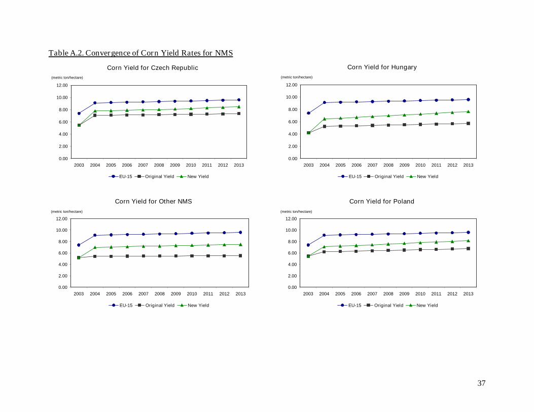
Other NMSWheat 3211.92 -5.66 9.14 53.88Corn 1096.74 8.09 1.87 38.91Barley 2520.99 -4.72 20.30 93.08

PolandWheat 9564.82 -2.80 -4.44 28.72Corn 1971.90 1.42 6.28 26.26Barley 3419.99 -1.29 0.46 20.17

22

Table 6. Impact of scenarios on consumption (10-year average)Baseline


Scenario 2(percent)

Scenario 3(percent)

EU-15Wheat 96328.88 -0.01 0.00 0.03Corn 42194.42 0.00 -0.01 -0.01Barley 47873.41 -0.01 0.01 0.10

WorldWheat 624764.40 -0.01 0.02 0.55Corn 678730.84 0.01 -0.01 0.10Barley 151206.41 -0.03 0.16 1.16

Czech RepublicWheat 3139.94 1.51 -6.37 -6.19Corn 613.68 -2.30 -3.69 -3.74Barley 1421.58 3.73 -0.47 0.05

HungaryWheat 3131.73 2.76 -5.76 -5.58Corn 4037.48 -0.09 -4.78 -4.78Barley 429.72 15.10 -15.29 -14.11

Other NMSWheat 4308.14 4.21 -0.62 -0.60Corn 2145.15 -2.19 -2.38 -2.41Barley 3373.28 0.68 -5.48 -5.36

PolandWheat 8757.18 2.40 4.51 4.63Corn 2207.33 -0.57 -3.47 -3.46Barley 3203.06 0.51 1.54 1.69

23

Table 7. Impact of scenarios on net trade (10-year average)Baseline


Scenario 2(percent)

Scenario 3(percent)

EU-15Wheat 8263.99 0.35 -0.25 -2.48Corn -3498.78 0.02 -0.03 -0.14Barley 3869.72 0.41 -0.85 -4.17

WorldWheat 199335.78 -0.26 0.57 2.78Corn 165340.19 -0.02 -0.08 -0.24Barley 29437.93 1.25 -4.09 -10.08

Czech RepublicWheat 686.75 -24.57 70.70 160.22Corn -99.04 -22.11 -41.88 -98.10Barley 952.06 -10.76 11.85 41.24

HungaryWheat 706.18 -27.48 56.36 223.51Corn 1357.73 2.41 35.00 167.63Barley 498.24 -18.59 23.18 82.54

Other NMSWheat -1138.81 34.28 -29.24 -156.99Corn -1076.62 -12.48 -7.36 -45.35Barley -862.78 17.49 -83.32 -296.63

PolandWheat 778.56 -66.72 -118.43 325.58Corn -229.02 -15.66 -79.33 -206.85Barley 210.44 -51.58 -101.66 577.32

In Scenario 1, trade policies of the NMS were harmonized with that of the EU-15. Table

1 shows pre- and post-accession tariff rates. Some tariff rates increase in the NMS while others

decrease, leading to different responses on the part of producers and consumers.

In Scenario 1, wheat prices decrease in all the NMS, leading to lower production and

higher consumption levels. Net exports of the Czech Republic, Hungary, and Poland decrease,

although these countries still remain net exporters. The Other NMS group was a net importer of

24

wheat in the baseline. With the decrease in production and increase in consumption, their net

imports increase, showing a positive percentage change in net trade.

In Hungary, production of corn increases slightly, although the corn price decreases. As

the decrease in corn price is lower on average than the decrease in wheat and barley prices,

producers switch to corn. Consumption of corn is lower despite lower prices, as consumers

switch to wheat and barley. All this leads to a rise in Hungary’s net exports of cornin the

Scenario 1. The price of corn rises in all of the other NMS, leading to higher production and

lower consumption. The nine other NMS were net importers of corn in the baseline. In Scenario

1, their net imports decrease, thus leading to a negative sign in the percentage change of net

trade.

The barley price decreases in all of the NMS, leading to lower production and higher

consumption levels in Scenario 1. Barley net exports are lower in the Czech Republic, Hungary,

and Poland. Being a net importer of barley in the baseline, the Other NMS group increases its net

imports, causing a positive sign in the percentage change of net trade.

The impact of Scenario 1 on production, consumption, and net trade is minimal in the

EU-15 and world grain markets. The prices of all three crops increase in the EU-15 and world

markets because of the decrease in net exports of the NMS that decreases the supply in the world

markets.

In Scenario 2, full accession of the NMS to the EU-15 is implemented. Tables 2 and 3

present the additional changes in the agricultural and trade policies, such as assumptions of top-

up payments by the NMS, the decoupling rate, area payments, and export subsidies.

With the full accession, wheat prices increase in all of the NMS except Poland. As a

result, wheat consumption falls in the Czech Republic, Hungary, and Other NMS, and

25

production increases. The increase in production is smaller after 2009/10 with the introduction of

the set-aside. Net exports of Hungary and the Czech Republic increase, whereas net imports of

Other NMS fall. Poland experiences a fall in the wheat price, accompanied by an increase in

consumption and a decrease in production. This decreases wheat net exports of Poland. After

2009/10, Poland becomes a net importer of wheat in Scenario 2.

Wheat prices in the EU-15 and world markets decrease with the enlargement, though to a

lesser extent in the EU-15. Net exports from the NMS increase in the Scenario 2 until 2008/09.

After that, the set-aside is introduced, leading to lower net exports from the NMS. Still, on

average, net exports from the NMS increase, increasing the supply in world markets and

lowering prices on average. The impact on EU-15 and world consumption and production is

minimal.

Corn prices increase in all NMS, which causes a drop in corn consumption and an

increase in corn production in all NMS on average. The increase in production lessens after

2009/10 because of set-aside, and there is even a small decline in Other NMS. Czech Republic,

Other NMS, and Poland, which were net corn importers in the baseline, decrease their corn net

imports. Poland becomes a net exporter of corn in some years. Hungary, benefiting from the

higher production and lower consumption levels, increases its net exports considerably.

EU-15 and world corn prices are lower in Scenario 2, though the impact on consumption

and production is much smaller. The increase in corn production and the decrease in corn

consumption in total for the NMS turn them from a net importer in the baseline into a net

exporter in Scenario 2. The increased supply in world markets decreases the corn price, though

this impact is less than 1% on average in the world.

26

Barley prices increase in the Czech Republic, Hungary, and Other NMS. Consequently,

consumption falls and production increases in these NMS. The Czech Republic and Hungary, net

exporters of barley in the baseline, increase their net exports. The Other NMS group decreases its

net imports of barley. In Poland, barley prices fall with the accession, leading to higher

consumption. However, barley production increases despite falling prices until 2009/10. This is

due to the sharper decline in the wheat price in Poland with the accession. Producers partially

switch to barley, and production of barley is slightly higher. In 2009/10, the set-aside kicks in,

decreasing the barley production in Poland. Net exports of barley fall with the higher

consumption levels.

Accession increases barley production in the NMS and decreases consumption. The

resulting higher net exports of barley from the NMS decrease the barley price in world markets

and the EU-15. Thus, barley consumption is slightly higher in the EU-15 and barley production

is lower. Both production and consumption of world barley increase.

Scenario 3 combines EU enlargement with the technology transfer to the NMS. This

increases the supply response of the NMS compared to Scenario 2. Production in the NMS

increases for all three crops. The subsequent shift in the yield functions for the three crops in the

NMS is given in Appendix Tables A.1 through A.3. The responses of prices and consumption in

the Scenario 3 for the NMS are very similar to their responses in Scenario 2 with only the

accession. The larger increase in production increases the change in net trade values of the NMS

compared to Scenario 2. Wheat net exports of the Czech Republic, Hungary, and Poland increase

between 70% and 325% on average. The Other NMS group was a net importer of wheat in the

baseline. In Scenario 3, Other NMS becomes a net exporter of wheat. The Czech Republic’s and

the Other NMS group’s corn net imports decrease more than 50% on average. Hungary increases

27

its corn net exports by 1.7 million metric tons on average. Poland becomes a net exporter of corn

in Scenario 3. Barley net exports of the Czech Republic, Hungary, and Poland increase

significantly. Net importers of barley in the baseline, the Other NMS group becomes a net

exporter in the Scenario 3.

This substantial increase in the production of the three crops and the resulting change in

net trade of the NMS have larger impacts in the EU-15 and world grain markets. Prices of the

three crops decrease more in the EU-15 and world markets. On average, the world wheat price

decreases nearly 7%, the corn price decreases approximately 5%, and the barley price decreases

the most, at 15%. The impact on world production and consumption are smaller compared with

the prices but larger compared with Scenario 2.

In Scenario 3, the prices in the EU decrease more than they did in Scenario 2. Thus, the

NMS face lower prices compared with Scenario 2. Production and consumption in the EU-15

change minimally, though the net exports of wheat decrease 2.5% on average and net exports of

barley decrease 4% on average. Corn net imports decrease 0.14% on average.

Tables 8 through 10 present the change in welfare in the NMS for each scenario. The

detailed welfare changes for each crop are given in Appendix Tables C.1 through C.3. The

change in welfare is computed for the marketing year 2013/14 and reported in thousand U.S.

dollars at 1995 prices.

In Scenario 1, all NMS have a negative change in welfare as seen in Table 8. The loss of

welfare for the NMS ranges between US$6,358 and US$20,697. As can be seen in Table 8, the

lower prices in the NMS affect producers negatively and the change in producer surplus is

negative for all NMS. However, consumers benefit from the harmonization of trade policies with

the EU-15. The EV is positive for all NMS.

28

Table 9 shows the change in welfare from Scenario 2, i.e., accession without the

technology transfer. Czech Republic has a net welfare gain of US$428,450. Hungary gains

US$366,730, Other NMS gains US$429,632, and Poland gains US$467,797. The main

component of the welfare gain for NMS is the increase in producer surplus. Producers in the

NMS benefit from higher prices, whereas consumers are worse off in this scenario, except for

Poland where the wheat and barley prices decrease. The EV is negative in all NMS, except for

Poland. Export subsidy expenditures, though benefiting exporters and producers, decrease the net

welfare gain of the NMS. The change in tariff revenue is negative for all NMS except for Other

NMS. In total, the NMS gain from accession to the EU, but the producers are the main

beneficiaries of this enlargement.

Table 8. Welfare effects of Scenario 1 in grains market (1000 US$ at 1995 prices for 2013/14)

CountryChange in

Producer SurplusEquivalentVariation

Change in ExportSubsidy

Change in TariffRevenue

Net Change inWelfare

Czech Republic -13522.52 2431.97 0.00 -16.25 -11106.80

Hungary -9258.87 2363.79 0.00 -11.94 -6907.02

Other NMS* -26608.82 5641.79 0.00 0.00 -20697.03

Poland -7676.25 1317.79 0.00 0.00 -6358.46*Other NMS includes Cyprus, Estonia, Latvia, Lithuania, Malta, Slovakia, and Slovenia.


CountryChange in





Czech Republic 570666.44 -76214.68 65976.96 -23.81 428450.99

Hungary 452051.62 -54191.20 31104.50 -25.30 366730.62

Other NMS* 503295.68 -67364.73 6301.54 2.85 429632.26

Poland 413900.10 54148.58 249.12 -1.57 467797.99*Other NMS includes Cyprus, Estonia, Latvia, Lithuania, Malta, Slovakia, and Slovenia.

29

Incorporating technology transfer to the accession scenario increases the net welfare

gains of the NMS as seen in Table 10. The Czech Republic increases its welfare gain to

US$571,604. Hungary gains US$582,633, Other NMS gains US$720,837, and Poland gains

US$773,743. In this scenario, the increase in export subsidy expenditures is much higher

compared to Scenario 2 for all NMS except for Poland because of the higher production and

export levels. As previously discussed, prices in the EU decrease more in Scenario 3. Therefore,

the NMS face lower prices compared with Scenario 2, though much higher compared with the

baseline. Thus, the loss of consumer welfare is less for most of the NMS. Poland has a higher

EV, and Polish consumers benefit more in Scenario 3. However, the increase in production and

therefore the fall in prices are not enough to generate a positive EV. The change in producer

surplus is higher in Scenario 3 for all NMS because of higher production levels, despite the fall

in prices relative to Scenario 2. Again, the producers in the NSM are the major beneficiaries of

technology transfer and accession to the EU though the welfare loss to consumers is less.

When comparing results for welfare in Scenarios 2 and 3, it is necessary to remember the

immiserizing growth literature. This literature shows that changes in terms of trade or policy

distortions may decrease the welfare in a country after a technical change occurs. In this study,


CountryChange in





Czech Republic 726782.86 -73820.59 81346.55 -11.11 571604.61

Hungary 695933.01 -52853.34 60446.19 0.14 582633.62

Other NMS* 835283.25 -64796.79 49679.77 30.59 720837.28

Poland 715773.24 58207.50 235.31 -1.59 773743.84* Other NMS includes Cyprus, Estonia, Latvia, Lithuania, Malta, Slovakia, and Slovenia.

30

lower prices generated by the supply shift were not large enough to create a negative change in

producer surplus in the NMS. The export subsidy expenditures in Scenario 3 compared with

those in Scenario 2 were much higher but not large enough to compensate for the increase in

producer surplus and to lead to immiserizing growth. Thus, immiserizing growth does not occur

in this accession and technology transfer scenario.

Conclusions

This study analyzes the impacts of EU enlargement and technology transfer on the EU,

the NMS, and world grain markets. To this end, a multi-market, non-spatial, partial-equilibrium

model of world grain markets for the EU-15, the NMS, and other major countries and regions

was used. First, a benchmark scenario is set up that includes the 2003 CAP reform of the EU.

Then, two scenarios that incorporate two different phases of the EU enlargement are run. A third

scenario includes full accession of the NMS to the EU-15 as well as technology transfer that is

incorporated into the model of the third scenario in the form of a convergence of grain yields in

the NMS to the average yield level in the EU-15. The consequent welfare changes in the

acceding countries are computed for each scenario.

The first two scenario results show that the impact of EU enlargement on the world grain

markets is minor. However, a scenario that combines the enlargement with the technology

transfer gives a different outcome. The impact on world grain markets is larger as seen in the

much lower world grain prices.

In the EU-15, accession leads to lower grain prices and lower net exports. The effect on

production and consumption is minimal. On the other hand, Scenario 3, which generates a much

bigger supply shift in the NMS, affects EU grain markets to a greater extent. The decrease in EU

31

grain prices is higher, which in turn decreases the price hike that most NMS face in the aftermath

of the accession.

The NMS have a net welfare gain from the accession to the EU. The producers in the

NMS are the beneficiaries of the accession, whereas consumers face a welfare loss because of

increasing prices, except in the case of Poland. This welfare gain increases considerably when

technology transfer from the EU-15 to the NMS is taken into consideration. In Scenario 3,

technology transfer, combined with the accession, increases the supply response of producers

and the change in producer surplus in Scenario 3 is much higher than in Scenario 2. Despite

falling prices in the EU, producers more than compensate with the higher supply response and

increase their welfare gain. The lower prices compared with Scenario 2 help consumers and the

loss of welfare is smaller in Scenario 3. In Scenarios 2 and 3, producers and exporters also gain

from export subsidies that decrease net welfare gain.

This study also explores the possibility of immiserizing growth in the grain sectors of the

NMS after acceding to the EU. The possibility of deterioration in the terms of trade and the use

of export subsidies create conditions that may lead to immiserizing growth, i.e., a negative net

welfare change after technical change. The computation of welfare changes in Scenario 3 shows

that this is not the case. In Scenario 3, lower prices generated by the supply shift were not large

enough to create a negative change in producer surplus in the NMS. The export subsidy

expenditures in Scenario 3 were much higher than in Scenario 2 but not high enough to

compensate for the increase in producer surplus and lead to immiserizing growth. Thus,

immiserizing growth does not occur in this scenario.

32

References

Agnew, Gates K., 1998. Linquad: An Incomplete Demand System Approach to Demand

Estimation and Exact Welfare Measures. Master’s Thesis, University of Arizona.

Alston, Julian M., Martin, Will J., 1995. Reversal of Fortune: Immiserizing Technical Change in

Agriculture. American Journal of Agricultural Economics 77, 251-259.

Bevan, Alan A., Estrin, Saul, 2004. The Determinants of Foreign Direct Investment into

European Transition Economies. Journal of Comparative Economics 32, 775-787.

Bhagwati, Jagdish M., 1958. Immiserizing Growth: A Geometrical Note. Review of Economic

Studies 25, 201-205.

Duczmal, Karol W., 2001. Agricultural Research and Technology Transfer to Rural

Communities in CEEC, CIS and Other Countries in Transition. In: Seed Policy and

Programmes for the Central and Eastern European Countries, Commonwealth of

Independent States and Other Countries in Transition. FAO Plant Production and

Protection Paper, Rome.

Fabiosa, Jacinto F., Beghin, John C., Dong, Fengxia, Elobeid, Amani, Fuller, Frank, Matthey,

Holger, Tokgoz, Simla, and Wailes, Eric. (2005). The Impact of the European

Enlargement and Common Agricultural Policy Reforms on Agricultural Markets: Much

Ado about Nothing? Working Paper 05-WP 382. Center for Agricultural and Rural

Development, Iowa State University, Ames, Iowa.

Food and Agricultural Policy Research Institute (FAPRI), 2005. Elasticities online database.

http://www.fapri.iastate.edu/tools/elasticity.aspx. Iowa State University, Ames, Iowa.

Heffer, Patrick, 2001. Biotechnology: A Modern Toll for Food Production Improvement. In:

Seed Policy and Programmes for the Central and Eastern European Countries,

33

Commonwealth of Independent States and Other Countries in Transition. FAO Plant

Production and Protection Paper, Rome.

Heinrich, István, 2001. Which Kind of Technology Is Suitable in Hungary? In: Tillack, Peter,

Fiege Ulrich (Eds.), Agricultural Technology and Economic Development of Central and

Eastern Europe, IAMO Workshop, Halle.

Jensen, Hans G., Frandsen, Soren E., 2003. Implications of EU Accession of Ten New Members

The Copenhagen Agreement. Working Paper. Danish Research Institute of Food

Economics (FOI).

Johnson, Harry G., 1958. International Trade and Economic Growth. London: George Allen and

Unwin.

Johnson, Harry G., 1967. The Possibility of Income Losses from Increased Efficiency and Factor

Accumulation in the Presence of Tariffs. Economic Journal 77, 151-154.

Josling, Timothy, Tangermann, Stefan, and Walkenhorst, Peter, 1997. Foreign Direct Investment

and Trade in Eastern Europe: The Creation of a Unified European Economy. The

Agricultural and Food Sectors. Working Paper No. ½, Institute of Agricultural

Economics, University of Göttingen.

LaFrance, Jeffrey T., 1998. The LINQUAD Incomplete Demand Model. Working Paper,

Department of Agricultural and Resource Economics, University of California, Berkeley.

LaFrance, Jeffrey T., Beatty, Timothy K.M., Pope, Rulon D., Agnew, Gates K., 2002.

Information Theoretic Measures of the Income Distribution in Food Demand. Journal of

Econometrics 107, 235-257.

Pawlak, Jan, Muzalewski, Aleksander, 2001. Farm Machinery and Market Services in

Poland. In: Tillack, Peter, Fiege, Ulrich (Eds.), Agricultural Technology and Economic

34

Development of Central and Eastern Europe, IAMO Workshop, Halle.

Pouliquen, Alain, 2001. Competitiveness and Farm Incomes in the CEEC Agri-Food Sectors.

European Commission Report, DG Agriculture, Brussels.

Sinani, Evis, Meyer, Klaus E., 2004. Spillovers of Technology Transfer from FDI: The Case of

Estonia. Journal of Comparative Economics 32, 445-466.

Turi, János, 2001. Role of Private Companies in the Seed Production and Distribution Systems in

CEEC, CIS, and other Countries in Transition: Hungarian Experience. In: Seed Policy

and Programmes for the Central and Eastern European Countries, Commonwealth of

Independent States and Other Countries in Transition. FAO Plant Production and

Protection Paper, Rome.

Tyers, Rod, 1993. Agricultural Sector Impacts of Economic Reform in Greater Europe and the

Former Soviet Union. Journal of Economic Integration 8, 245-277.

35

Endnotes

1. Cyprus, Czech Republic, Estonia, Hungary, Latvia, Lithuania, Malta, Poland, Slovakia, and

Slovenia.

2. All welfare calculations are computed for the year 2013/14, which is the marketing year that

starts in 2013 and ends in 2014.

3. Third-country exports include exports to all countries except the EU-15 and the 10 NMS.

4. See Bhagwati (1958) and Johnson (1958) for a discussion of immiserizing growth in the

absence of distortions when demand is inelastic.

36

Appendix Tables

Table A.1. Convergence of Wheat Yield Rates for NMS

Wheat Yield for Czech Republic

0.00

1.00

2.00

3.00

4.00

5.00

6.00

7.00

2003 2004 2005 2006 2007 2008 2009 2010 2011 2012 2013

(metric ton/hectare)

EU-15 Original Yield New Yield

Wheat Yield for Hungary

0.00

1.00

2.00

3.00

4.00

5.00

6.00

7.00

2003 2004 2005 2006 2007 2008 2009 2010 2011 2012 2013



Wheat Yield for Other NMS

0.00

1.00

2.00

3.00

4.00

5.00

6.00

7.00

2003 2004 2005 2006 2007 2008 2009 2010 2011 2012 2013



Wheat Yield for Poland

0.00

1.00

2.00

3.00

4.00

5.00

6.00

7.00

2003 2004 2005 2006 2007 2008 2009 2010 2011 2012 2013



37

Table A.2. Convergence of Corn Yield Rates for NMS

Corn Yield for Czech Republic

0.00

2.00

4.00

6.00

8.00

10.00

12.00

2003 2004 2005 2006 2007 2008 2009 2010 2011 2012 2013



Corn Yield for Hungary

0.00

2.00

4.00

6.00

8.00

10.00

12.00

2003 2004 2005 2006 2007 2008 2009 2010 2011 2012 2013



Corn Yield for Other NMS

0.00

2.00

4.00

6.00

8.00

10.00

12.00

2003 2004 2005 2006 2007 2008 2009 2010 2011 2012 2013



Corn Yield for Poland

0.00

2.00

4.00

6.00

8.00

10.00

12.00

2003 2004 2005 2006 2007 2008 2009 2010 2011 2012 2013



38

Table A.3. Convergence of Barley Yield Rates for NMS

Barley Yield for Czech Republic

0.00

1.00

2.00

3.00

4.00

5.00

6.00

2003 2004 2005 2006 2007 2008 2009 2010 2011 2012 2013



Barley Yield for Hungary

0.00

1.00

2.00

3.00

4.00

5.00

6.00

2003 2004 2005 2006 2007 2008 2009 2010 2011 2012 2013



Barley Yield for Other NMS

0.00

1.00

2.00

3.00

4.00

5.00

6.00

2003 2004 2005 2006 2007 2008 2009 2010 2011 2012 2013



Barley Yield for Poland

0.00

1.00

2.00

3.00

4.00

5.00

6.00

2003 2004 2005 2006 2007 2008 2009 2010 2011 2012 2013



Table B.1. Impacts of EU Enlargement on Czech Republic Wheat

03/04 04/05 05/06 06/07 07/08 08/09 09/10 10/11 11/12 12/13 13/14

Area Harvested Baseline 650 746 786 802 812 829 845 862 882 900 919 Scenario 1 650 746 764 781 793 810 827 845 865 884 903 Scenario 2 650 746 834 848 864 878 847 861 880 896 914 Scenario 3 650 746 852 865 879 892 860 873 891 908 926 Impact of Scenario 1 (%) 0.00 0.00 -2.88 -2.60 -2.37 -2.21 -2.04 -1.92 -1.84 -1.79 -1.72 Impact of Scenario 2 (%) 0.00 0.00 6.08 5.77 6.38 5.94 0.35 -0.04 -0.23 -0.44 -0.60 Impact of Scenario 3 (%) 0.00 0.00 8.40 7.82 8.27 7.64 1.79 1.26 1.08 0.86 0.70

Yield Baseline 4.00 4.51 4.53 4.54 4.56 4.57 4.59 4.61 4.63 4.65 4.67 Scenario 1 4.00 4.48 4.50 4.51 4.53 4.55 4.57 4.59 4.61 4.63 4.65 Scenario 2 4.00 4.61 4.63 4.66 4.67 4.68 4.69 4.71 4.73 4.74 4.76 Scenario 3 4.00 5.18 5.19 5.21 5.23 5.23 5.25 5.29 5.33 5.37 5.41 Impact of Scenario 1 (%) 0.00 -0.71 -0.63 -0.58 -0.54 -0.50 -0.47 -0.46 -0.44 -0.43 -0.42 Impact of Scenario 2 (%) 0.00 2.24 2.40 2.56 2.49 2.37 2.23 2.17 2.10 2.05 1.95 Impact of Scenario 3 (%) 0.00 14.76 14.62 14.80 14.66 14.45 14.32 14.79 15.21 15.65 16.02

Production Baseline 2,600 3,366 3,559 3,643 3,700 3,790 3,877 3,972 4,080 4,183 4,288 Scenario 1 2,600 3,342 3,435 3,527 3,593 3,687 3,780 3,878 3,987 4,091 4,197 Scenario 2 2,600 3,442 3,866 3,951 4,034 4,110 3,977 4,057 4,156 4,250 4,345 Scenario 3 2,600 3,863 4,422 4,509 4,593 4,669 4,511 4,618 4,751 4,879 5,009 Impact of Scenario 1 (%) 0.00 -0.71 -3.49 -3.17 -2.90 -2.70 -2.51 -2.37 -2.28 -2.21 -2.13 Impact of Scenario 2 (%) 0.00 2.24 8.62 8.47 9.03 8.45 2.59 2.12 1.87 1.60 1.34 Impact of Scenario 3 (%) 0.00 14.76 24.25 23.77 24.14 23.19 16.37 16.24 16.46 16.65 16.83

Domestic Supply Baseline 3,298 3,764 3,935 4,057 4,159 4,286 4,405 4,527 4,645 4,758 4,871 Scenario 1 3,298 3,740 3,850 3,987 4,096 4,224 4,346 4,469 4,588 4,699 4,813 Scenario 2 3,298 3,840 4,120 4,203 4,310 4,420 4,325 4,440 4,556 4,663 4,770 Scenario 3 3,298 4,261 4,681 4,766 4,875 4,984 4,864 5,005 5,156 5,297 5,439 Impact of Scenario 1 (%) 0.00 -0.63 -2.18 -1.74 -1.53 -1.43 -1.33 -1.27 -1.24 -1.23 -1.19 Impact of Scenario 2 (%) 0.00 2.01 4.70 3.59 3.62 3.14 -1.81 -1.93 -1.93 -1.98 -2.06 Impact of Scenario 3 (%) 0.00 13.20 18.94 17.46 17.20 16.30 10.44 10.57 10.98 11.34 11.67

Feed Use Baseline 1,500 1,497 1,502 1,549 1,565 1,586 1,602 1,612 1,623 1,637 1,650 Scenario 1 1,500 1,541 1,537 1,581 1,596 1,615 1,629 1,638 1,649 1,662 1,675 Scenario 2 1,500 1,340 1,362 1,395 1,420 1,447 1,470 1,483 1,496 1,512 1,531 Scenario 3 1,500 1,345 1,366 1,399 1,423 1,451 1,474 1,486 1,499 1,515 1,534 Impact of Scenario 1 (%) 0.00 2.95 2.34 2.08 1.94 1.79 1.67 1.62 1.58 1.53 1.52 Impact of Scenario 2 (%) 0.00 -10.46 -9.32 -9.94 -9.30 -8.78 -8.22 -8.02 -7.85 -7.68 -7.23 Impact of Scenario 3 (%) 0.00 -10.16 -9.04 -9.68 -9.06 -8.56 -8.01 -7.81 -7.65 -7.48 -7.04

Consumption Baseline 3,100 3,061 3,071 3,122 3,137 3,156 3,168 3,168 3,169 3,174 3,175 Scenario 1 3,100 3,128 3,127 3,173 3,185 3,201 3,210 3,209 3,210 3,214 3,215 Scenario 2 3,100 2,841 2,865 2,896 2,922 2,951 2,974 2,978 2,983 2,991 3,001 Scenario 3 3,100 2,848 2,872 2,902 2,928 2,956 2,979 2,983 2,988 2,995 3,006 Impact of Scenario 1 (%) 0.00 2.21 1.82 1.64 1.54 1.43 1.35 1.31 1.29 1.25 1.25 Impact of Scenario 2 (%) 0.00 -7.17 -6.70 -7.21 -6.84 -6.50 -6.12 -5.99 -5.88 -5.78 -5.48 Impact of Scenario 3 (%) 0.00 -6.95 -6.49 -7.02 -6.66 -6.33 -5.96 -5.83 -5.72 -5.63 -5.33

Domestic Use Baseline 3,498 3,437 3,486 3,581 3,633 3,684 3,722 3,733 3,744 3,757 3,764 Scenario 1 3,498 3,543 3,586 3,676 3,722 3,768 3,801 3,810 3,819 3,830 3,836 Scenario 2 3,498 3,095 3,117 3,172 3,232 3,299 3,357 3,378 3,396 3,416 3,439 Scenario 3 3,498 3,107 3,129 3,184 3,244 3,309 3,367 3,387 3,406 3,425 3,448 Impact of Scenario 1 (%) 0.00 3.09 2.89 2.65 2.47 2.28 2.12 2.05 2.00 1.94 1.91 Impact of Scenario 2 (%) 0.00 -9.94 -10.58 -11.41 -11.02 -10.45 -9.82 -9.52 -9.29 -9.08 -8.64 Impact of Scenario 3 (%) 0.00 -9.61 -10.24 -11.09 -10.71 -10.17 -9.55 -9.26 -9.04 -8.84 -8.40

Ending Stocks Baseline 398 376 415 459 496 528 555 565 574 583 589 Scenario 1 398 415 459 503 537 567 591 600 609 616 621 Scenario 2 398 254 251 276 310 348 383 400 413 425 437 Scenario 3 398 259 257 281 316 353 388 404 418 430 442 Impact of Scenario 1 (%) 0.00 10.26 10.81 9.49 8.33 7.34 6.57 6.19 5.93 5.69 5.51 Impact of Scenario 2 (%) 0.00 -32.45 -39.36 -39.94 -37.42 -34.08 -30.93 -29.35 -28.11 -27.09 -25.73 Impact of Scenario 3 (%) 0.00 -31.23 -38.03 -38.73 -36.34 -33.12 -30.06 -28.51 -27.31 -26.31 -24.98

Net Trade Baseline -200 327 450 476 527 602 682 794 901 1,001 1,107 Scenario 1 -200 197 263 311 374 457 545 660 769 869 977 Scenario 2 -200 744 1,004 1,031 1,078 1,122 968 1,062 1,160 1,248 1,332 Scenario 3 -200 1,154 1,552 1,582 1,631 1,675 1,498 1,618 1,750 1,872 1,991 Impact of Scenario 1 (%) 0.00 -39.72 -41.47 -34.69 -29.09 -24.09 -20.15 -16.90 -14.71 -13.14 -11.76 Impact of Scenario 2 (%) 0.00 127.45 123.09 116.31 104.55 86.34 41.89 33.80 28.62 24.67 20.32 Impact of Scenario 3 (%) 0.00 252.74 245.09 232.00 209.63 178.32 119.47 103.85 94.13 87.08 79.90

(Thousand Hectares)

(Metric Tons per Hectare)

(Thousand Metric Tons)

39

Table B.2. Impacts of EU Enlargement on Czech Republic Corn

03/04 04/05 05/06 06/07 07/08 08/09 09/10 10/11 11/12 12/13 13/14

Area Harvested Baseline 80 78 71 69 69 68 72 74 74 73 73 Scenario 1 80 78 73 71 70 70 73 75 75 75 74 Scenario 2 80 78 74 73 72 72 75 76 76 76 76 Scenario 3 80 78 74 73 73 72 75 77 77 77 77 Impact of Scenario 1 (%) 0.00 0.00 1.94 2.15 2.16 2.08 1.89 1.77 1.74 1.75 1.72 Impact of Scenario 2 (%) 0.00 0.00 3.75 4.50 4.94 4.97 3.56 3.12 3.27 3.41 3.42 Impact of Scenario 3 (%) 0.00 0.00 4.28 5.25 5.83 5.96 4.52 4.10 4.31 4.52 4.58

Yield Baseline 5.44 7.00 7.02 7.04 7.07 7.10 7.13 7.17 7.20 7.24 7.28 Scenario 1 5.44 7.01 7.03 7.05 7.08 7.11 7.14 7.18 7.22 7.26 7.30 Scenario 2 5.44 7.06 7.08 7.11 7.14 7.16 7.19 7.23 7.27 7.31 7.35 Scenario 3 5.44 7.78 7.82 7.89 7.95 8.02 8.08 8.18 8.27 8.36 8.46 Impact of Scenario 1 (%) 0.00 0.25 0.20 0.19 0.18 0.18 0.17 0.17 0.17 0.17 0.17 Impact of Scenario 2 (%) 0.00 0.95 0.95 0.98 0.95 0.92 0.89 0.88 0.88 0.86 0.84 Impact of Scenario 3 (%) 0.00 11.22 11.52 12.07 12.51 12.94 13.41 14.10 14.79 15.43 16.10

Production Baseline 435 543 500 489 485 485 513 530 530 531 533 Scenario 1 435 545 511 500 496 496 524 541 540 541 543 Scenario 2 435 549 524 516 514 513 536 552 552 554 556 Scenario 3 435 604 582 576 577 580 609 630 634 641 647 Impact of Scenario 1 (%) 0.00 0.25 2.14 2.35 2.35 2.25 2.06 1.95 1.92 1.92 1.90 Impact of Scenario 2 (%) 0.00 0.95 4.73 5.52 5.94 5.94 4.49 4.03 4.18 4.30 4.29 Impact of Scenario 3 (%) 0.00 11.22 16.29 17.95 19.07 19.67 18.54 18.78 19.73 20.64 21.41

Domestic Supply Baseline 572 575 521 509 506 507 536 554 554 555 558 Scenario 1 572 577 531 520 517 517 546 564 563 565 567 Scenario 2 572 581 541 532 531 531 555 571 572 574 576 Scenario 3 572 636 599 593 594 598 627 650 654 661 668 Impact of Scenario 1 (%) 0.00 0.24 1.87 2.07 2.07 1.99 1.82 1.72 1.69 1.69 1.67 Impact of Scenario 2 (%) 0.00 0.90 3.83 4.47 4.81 4.81 3.50 3.11 3.26 3.37 3.38 Impact of Scenario 3 (%) 0.00 10.59 14.93 16.40 17.39 17.94 16.95 17.23 18.14 19.01 19.75

Feed Use Baseline 370 407 432 463 488 511 531 552 569 586 602 Scenario 1 370 403 424 453 476 498 517 537 553 569 584 Scenario 2 370 401 420 447 468 488 506 524 539 554 568 Scenario 3 370 401 420 447 468 488 506 524 539 554 568 Impact of Scenario 1 (%) 0.00 -1.09 -1.68 -2.09 -2.36 -2.53 -2.66 -2.74 -2.81 -2.85 -2.90 Impact of Scenario 2 (%) 0.00 -1.59 -2.66 -3.47 -4.04 -4.46 -4.78 -5.03 -5.26 -5.42 -5.56 Impact of Scenario 3 (%) 0.00 -1.60 -2.67 -3.49 -4.07 -4.49 -4.80 -5.06 -5.29 -5.45 -5.59

Consumption Baseline 450 511 530 562 586 610 630 651 669 686 702 Scenario 1 450 504 521 551 573 595 614 634 651 668 683 Scenario 2 450 502 518 546 566 586 604 622 638 653 668 Scenario 3 450 502 518 545 566 586 604 622 638 653 668 Impact of Scenario 1 (%) 0.00 -1.42 -1.74 -2.07 -2.27 -2.41 -2.50 -2.56 -2.63 -2.66 -2.69 Impact of Scenario 2 (%) 0.00 -1.75 -2.16 -2.99 -3.39 -3.82 -4.11 -4.37 -4.62 -4.77 -4.91 Impact of Scenario 3 (%) 0.00 -1.81 -2.21 -3.05 -3.45 -3.87 -4.16 -4.42 -4.67 -4.82 -4.96

Domestic Use Baseline 482 532 551 584 609 633 654 675 693 710 727 Scenario 1 482 524 541 571 594 617 637 657 675 691 707 Scenario 2 482 519 535 563 584 605 624 642 658 674 689 Scenario 3 482 519 535 562 584 605 623 642 658 673 688 Impact of Scenario 1 (%) 0.00 -1.55 -1.84 -2.14 -2.32 -2.45 -2.53 -2.59 -2.65 -2.68 -2.72 Impact of Scenario 2 (%) 0.00 -2.38 -2.85 -3.65 -3.99 -4.35 -4.60 -4.82 -5.05 -5.18 -5.29 Impact of Scenario 3 (%) 0.00 -2.42 -2.89 -3.69 -4.03 -4.40 -4.64 -4.86 -5.09 -5.22 -5.33

Ending Stocks Baseline 32 21 21 22 22 23 24 24 24 25 25 Scenario 1 32 20 20 21 21 22 23 23 23 24 24 Scenario 2 32 18 17 17 18 19 20 20 20 20 21 Scenario 3 32 18 17 17 18 19 20 20 20 21 21 Impact of Scenario 1 (%) 0.00 -4.62 -4.35 -4.07 -3.76 -3.52 -3.38 -3.29 -3.33 -3.23 -3.31 Impact of Scenario 2 (%) 0.00 -17.38 -20.32 -20.68 -19.68 -18.50 -17.48 -17.07 -16.91 -16.47 -16.16 Impact of Scenario 3 (%) 0.00 -17.18 -20.09 -20.46 -19.49 -18.32 -17.31 -16.91 -16.76 -16.32 -16.01

Net Trade Baseline 90 43 -29 -75 -102 -126 -117 -121 -139 -155 -169 Scenario 1 90 53 -10 -52 -78 -100 -91 -94 -111 -127 -140 Scenario 2 90 61 6 -31 -53 -74 -68 -71 -86 -100 -112 Scenario 3 90 117 64 30 10 -7 4 8 -3 -13 -21 Impact of Scenario 1 (%) 0.00 22.15 -67.57 -30.94 -24.12 -20.36 -22.45 -22.36 -19.94 -18.31 -17.16 Impact of Scenario 2 (%) 0.00 41.08 -121.31 -59.05 -47.64 -41.33 -41.63 -41.22 -38.09 -35.76 -33.81 Impact of Scenario 3 (%) 0.00 170.41 -318.87 -140.82 -110.25 -94.55 -103.39 -106.25 -97.52 -91.92 -87.85

(Thousand Hectares)



40

Table B.3. Impacts of EU Enlargement on Czech Republic Barley

03/04 04/05 05/06 06/07 07/08 08/09 09/10 10/11 11/12 12/13 13/14

Area Harvested Baseline 550 524 612 614 612 621 618 612 610 610 609 Scenario 1 550 524 598 601 600 610 608 602 600 600 599 Scenario 2 550 524 631 655 657 671 636 622 620 617 614 Scenario 3 550 524 643 669 671 684 648 632 630 627 624 Impact of Scenario 1 (%) 0.00 0.00 -2.34 -2.16 -2.07 -1.86 -1.76 -1.66 -1.58 -1.55 -1.51 Impact of Scenario 2 (%) 0.00 0.00 3.00 6.63 7.27 8.00 2.90 1.67 1.60 1.15 0.82 Impact of Scenario 3 (%) 0.00 0.00 4.98 8.95 9.59 10.15 4.78 3.38 3.29 2.85 2.53



Domestic Supply Baseline 2,250 2,098 2,423 2,441 2,443 2,492 2,494 2,487 2,497 2,512 2,524 Scenario 1 2,250 2,087 2,358 2,382 2,387 2,440 2,446 2,442 2,453 2,469 2,482 Scenario 2 2,250 2,114 2,529 2,629 2,649 2,715 2,590 2,550 2,556 2,560 2,563 Scenario 3 2,250 2,311 2,812 2,931 2,949 3,014 2,868 2,830 2,843 2,855 2,868 Impact of Scenario 1 (%) 0.00 -0.55 -2.66 -2.44 -2.30 -2.08 -1.95 -1.84 -1.75 -1.71 -1.65 Impact of Scenario 2 (%) 0.00 0.76 4.38 7.70 8.41 8.95 3.82 2.53 2.37 1.89 1.56 Impact of Scenario 3 (%) 0.00 10.16 16.05 20.04 20.69 20.95 15.00 13.76 13.87 13.66 13.63

Feed Use Baseline 1,300 1,029 907 857 846 851 865 878 885 894 907 Scenario 1 1,300 1,062 952 909 899 904 916 927 933 941 953 Scenario 2 1,300 1,058 917 865 844 848 863 878 891 905 921 Scenario 3 1,300 1,061 923 872 851 855 870 884 897 912 927 Impact of Scenario 1 (%) 0.00 3.19 4.96 6.02 6.24 6.16 5.89 5.64 5.48 5.30 5.08 Impact of Scenario 2 (%) 0.00 2.76 1.12 0.91 -0.15 -0.35 -0.29 0.02 0.70 1.23 1.48 Impact of Scenario 3 (%) 0.00 3.13 1.73 1.68 0.66 0.46 0.49 0.78 1.44 1.95 2.18

Consumption Baseline 1,900 1,544 1,461 1,395 1,389 1,390 1,402 1,406 1,406 1,408 1,414 Scenario 1 1,900 1,587 1,511 1,453 1,447 1,448 1,458 1,460 1,459 1,460 1,464 Scenario 2 1,900 1,563 1,453 1,389 1,371 1,373 1,386 1,393 1,401 1,408 1,416 Scenario 3 1,900 1,569 1,459 1,397 1,379 1,381 1,393 1,400 1,408 1,415 1,423 Impact of Scenario 1 (%) 0.00 2.74 3.43 4.13 4.16 4.13 3.96 3.83 3.75 3.65 3.52 Impact of Scenario 2 (%) 0.00 1.24 -0.56 -0.42 -1.34 -1.25 -1.18 -0.92 -0.39 -0.02 0.16 Impact of Scenario 3 (%) 0.00 1.59 -0.10 0.13 -0.77 -0.68 -0.63 -0.38 0.14 0.50 0.67

Domestic Use Baseline 1,975 1,604 1,520 1,456 1,453 1,458 1,473 1,478 1,479 1,482 1,489 Scenario 1 1,975 1,648 1,573 1,516 1,514 1,518 1,531 1,534 1,534 1,536 1,541 Scenario 2 1,975 1,620 1,505 1,442 1,426 1,431 1,447 1,456 1,466 1,474 1,484 Scenario 3 1,975 1,626 1,512 1,450 1,434 1,440 1,456 1,465 1,474 1,482 1,492 Impact of Scenario 1 (%) 0.00 2.77 3.46 4.15 4.16 4.11 3.93 3.79 3.71 3.61 3.47 Impact of Scenario 2 (%) 0.00 1.02 -0.99 -0.97 -1.91 -1.82 -1.72 -1.45 -0.90 -0.52 -0.34 Impact of Scenario 3 (%) 0.00 1.38 -0.52 -0.40 -1.33 -1.24 -1.16 -0.90 -0.37 0.00 0.18


Net Trade Baseline 275 494 903 986 990 1,034 1,022 1,010 1,018 1,030 1,035 Scenario 1 275 438 786 866 873 923 915 908 919 933 942 Scenario 2 275 494 1,024 1,188 1,223 1,284 1,142 1,094 1,091 1,085 1,079 Scenario 3 275 685 1,299 1,481 1,515 1,574 1,413 1,365 1,370 1,373 1,376 Impact of Scenario 1 (%) 0.00 -11.30 -12.97 -12.17 -11.78 -10.80 -10.41 -10.07 -9.68 -9.37 -9.02 Impact of Scenario 2 (%) 0.00 -0.10 13.42 20.50 23.57 24.13 11.81 8.36 7.12 5.37 4.29 Impact of Scenario 3 (%) 0.00 38.64 43.94 50.22 53.02 52.21 38.30 35.21 34.54 33.32 32.98


(Thousand Hectares)


41

Table. B.4. Impacts of EU Enlargement on Hungary Wheat

03/04 04/05 05/06 06/07 07/08 08/09 09/10 10/11 11/12 12/13 13/14

Area Harvested Baseline 1,200 1,093 1,084 1,078 1,067 1,063 1,062 1,058 1,057 1,055 1,053 Scenario 1 1,200 1,093 1,062 1,052 1,042 1,039 1,038 1,035 1,034 1,033 1,032 Scenario 2 1,200 1,093 1,144 1,149 1,147 1,147 1,092 1,076 1,074 1,071 1,068 Scenario 3 1,200 1,093 1,170 1,180 1,179 1,180 1,125 1,109 1,107 1,104 1,102 Impact of Scenario 1 (%) 0.00 0.00 -2.09 -2.41 -2.33 -2.29 -2.27 -2.19 -2.14 -2.11 -2.07 Impact of Scenario 2 (%) 0.00 0.00 5.53 6.65 7.58 7.84 2.82 1.76 1.67 1.52 1.36 Impact of Scenario 3 (%) 0.00 0.00 7.88 9.49 10.57 10.95 5.91 4.80 4.76 4.67 4.57




Feed Use Baseline 900 861 882 922 954 983 997 1,011 1,018 1,027 1,034 Scenario 1 900 911 936 975 1,007 1,036 1,047 1,061 1,068 1,075 1,081 Scenario 2 900 802 804 832 859 886 904 922 933 944 957 Scenario 3 900 805 808 836 863 889 908 925 936 947 960 Impact of Scenario 1 (%) 0.00 5.80 6.12 5.75 5.52 5.41 5.10 4.94 4.82 4.66 4.56 Impact of Scenario 2 (%) 0.00 -6.86 -8.82 -9.77 -9.97 -9.91 -9.25 -8.81 -8.40 -8.09 -7.51 Impact of Scenario 3 (%) 0.00 -6.51 -8.43 -9.39 -9.59 -9.55 -8.91 -8.48 -8.07 -7.78 -7.20




Net Trade Baseline 450 828 757 704 673 667 659 668 686 700 720 Scenario 1 450 663 550 494 468 464 463 477 498 517 539 Scenario 2 450 1,102 1,217 1,232 1,235 1,243 1,020 981 989 991 988 Scenario 3 450 1,936 2,241 2,327 2,386 2,452 2,215 2,206 2,261 2,310 2,351 Impact of Scenario 1 (%) 0.00 -19.91 -27.35 -29.74 -30.43 -30.48 -29.67 -28.57 -27.32 -26.23 -25.10 Impact of Scenario 2 (%) 0.00 33.06 60.84 75.09 83.66 86.32 54.87 46.88 44.18 41.52 37.21 Impact of Scenario 3 (%) 0.00 133.79 196.01 230.68 254.73 267.47 236.19 230.15 229.70 229.83 226.56

(Thousand Hectares)



42

Table B.5. Impacts of EU Enlargement on Hungary Corn

03/04 04/05 05/06 06/07 07/08 08/09 09/10 10/11 11/12 12/13 13/14

Area Harvested Baseline 1,100 1,075 985 955 994 1,005 1,008 1,006 1,004 1,002 1,000 Scenario 1 1,100 1,075 993 963 1,002 1,013 1,016 1,014 1,012 1,010 1,008 Scenario 2 1,100 1,075 1,018 996 1,038 1,051 1,047 1,044 1,044 1,043 1,041 Scenario 3 1,100 1,075 1,035 1,018 1,063 1,077 1,073 1,071 1,071 1,070 1,069 Impact of Scenario 1 (%) 0.00 0.00 0.76 0.81 0.77 0.75 0.77 0.78 0.77 0.80 0.79 Impact of Scenario 2 (%) 0.00 0.00 3.30 4.29 4.44 4.59 3.90 3.83 4.00 4.09 4.03 Impact of Scenario 3 (%) 0.00 0.00 5.04 6.62 6.90 7.17 6.49 6.43 6.66 6.83 6.83


Production Baseline 4,600 5,540 5,128 5,020 5,279 5,393 5,458 5,501 5,544 5,589 5,635 Scenario 1 4,600 5,529 5,156 5,050 5,310 5,425 5,492 5,536 5,581 5,627 5,674 Scenario 2 4,600 5,614 5,368 5,307 5,589 5,718 5,745 5,784 5,838 5,887 5,930 Scenario 3 4,600 6,930 6,799 6,823 7,265 7,513 7,615 7,737 7,882 8,021 8,151 Impact of Scenario 1 (%) 0.00 -0.20 0.54 0.61 0.59 0.58 0.62 0.64 0.65 0.68 0.69 Impact of Scenario 2 (%) 0.00 1.35 4.67 5.72 5.87 6.01 5.25 5.14 5.30 5.34 5.24 Impact of Scenario 3 (%) 0.00 25.10 32.58 35.93 37.62 39.30 39.52 40.65 42.17 43.52 44.65

Domestic Supply Baseline 4,751 5,691 5,328 5,247 5,523 5,646 5,716 5,767 5,817 5,866 5,917 Scenario 1 4,751 5,680 5,361 5,286 5,562 5,685 5,757 5,810 5,859 5,910 5,961 Scenario 2 4,751 5,765 5,528 5,482 5,775 5,910 5,941 5,991 6,052 6,106 6,155 Scenario 3 4,751 7,081 6,960 6,999 7,451 7,706 7,812 7,945 8,096 8,241 8,377 Impact of Scenario 1 (%) 0.00 -0.19 0.63 0.75 0.71 0.70 0.73 0.73 0.73 0.75 0.75 Impact of Scenario 2 (%) 0.00 1.31 3.75 4.48 4.56 4.69 3.95 3.87 4.04 4.09 4.03 Impact of Scenario 3 (%) 0.00 24.44 30.62 33.39 34.92 36.50 36.68 37.75 39.19 40.49 41.57


Consumption Baseline 4,100 3,944 3,893 3,937 3,990 4,060 4,073 4,108 4,117 4,122 4,130 Scenario 1 4,100 3,939 3,893 3,936 3,990 4,059 4,070 4,104 4,111 4,116 4,123 Scenario 2 4,100 3,805 3,721 3,747 3,792 3,853 3,868 3,903 3,909 3,918 3,928 Scenario 3 4,100 3,805 3,721 3,746 3,792 3,853 3,868 3,903 3,909 3,918 3,928 Impact of Scenario 1 (%) 0.00 -0.13 -0.01 -0.01 -0.01 -0.04 -0.09 -0.10 -0.14 -0.14 -0.19 Impact of Scenario 2 (%) 0.00 -3.54 -4.41 -4.83 -4.96 -5.10 -5.04 -5.00 -5.04 -4.95 -4.89 Impact of Scenario 3 (%) 0.00 -3.54 -4.41 -4.83 -4.96 -5.10 -5.04 -5.00 -5.04 -4.95 -4.89

Domestic Use Baseline 4,251 4,144 4,120 4,180 4,243 4,318 4,340 4,380 4,394 4,404 4,417 Scenario 1 4,251 4,145 4,128 4,188 4,250 4,324 4,343 4,383 4,394 4,404 4,414 Scenario 2 4,251 3,965 3,896 3,932 3,985 4,049 4,075 4,116 4,128 4,143 4,159 Scenario 3 4,251 3,965 3,897 3,933 3,985 4,050 4,075 4,117 4,129 4,144 4,160 Impact of Scenario 1 (%) 0.00 0.01 0.20 0.19 0.18 0.14 0.08 0.06 0.00 -0.01 -0.06 Impact of Scenario 2 (%) 0.00 -4.33 -5.43 -5.93 -6.08 -6.21 -6.10 -6.03 -6.04 -5.92 -5.83 Impact of Scenario 3 (%) 0.00 -4.32 -5.42 -5.92 -6.07 -6.20 -6.09 -6.02 -6.03 -5.91 -5.82


Net Trade Baseline 500 1,546 1,208 1,066 1,280 1,328 1,376 1,387 1,423 1,462 1,500 Scenario 1 500 1,535 1,233 1,097 1,312 1,361 1,414 1,427 1,466 1,506 1,548 Scenario 2 500 1,800 1,632 1,549 1,790 1,861 1,867 1,875 1,924 1,963 1,996 Scenario 3 500 3,116 3,063 3,066 3,466 3,656 3,737 3,828 3,968 4,097 4,217 Impact of Scenario 1 (%) 0.00 -0.74 2.10 2.91 2.47 2.52 2.78 2.85 3.00 3.04 3.15 Impact of Scenario 2 (%) 0.00 16.43 35.04 45.30 39.82 40.11 35.65 35.14 35.18 34.26 33.06 Impact of Scenario 3 (%) 0.00 101.50 153.51 187.53 170.77 175.31 171.57 175.94 178.83 180.25 181.10

(Thousand Hectares)



43

Table B.6. Impacts of EU Enlargement on Hungary Barley

03/04 04/05 05/06 06/07 07/08 08/09 09/10 10/11 11/12 12/13 13/14

Area Harvested Baseline 300 285 317 314 314 311 311 308 307 306 305 Scenario 1 300 285 309 307 306 304 304 301 301 300 299 Scenario 2 300 285 332 337 337 337 321 316 315 313 311 Scenario 3 300 285 346 353 353 352 336 330 330 328 326 Impact of Scenario 1 (%) 0.00 0.00 -2.63 -2.43 -2.39 -2.26 -2.24 -2.12 -2.05 -2.01 -1.97 Impact of Scenario 2 (%) 0.00 0.00 4.67 7.33 7.47 8.19 3.27 2.55 2.72 2.36 2.02 Impact of Scenario 3 (%) 0.00 0.00 8.99 12.29 12.50 13.28 8.18 7.28 7.43 7.06 6.70


Production Baseline 830 839 934 932 935 934 938 935 938 942 945 Scenario 1 830 829 900 900 904 904 908 907 911 916 919 Scenario 2 830 849 995 1,017 1,023 1,028 984 973 977 977 976 Scenario 3 830 1,043 1,276 1,317 1,332 1,348 1,295 1,286 1,297 1,304 1,310 Impact of Scenario 1 (%) 0.00 -1.27 -3.70 -3.46 -3.36 -3.22 -3.13 -2.98 -2.88 -2.82 -2.73 Impact of Scenario 2 (%) 0.00 1.18 6.50 9.11 9.38 10.04 4.91 4.09 4.14 3.70 3.32 Impact of Scenario 3 (%) 0.00 24.27 36.61 41.29 42.50 44.25 38.12 37.59 38.34 38.44 38.59

Domestic Supply Baseline 912 901 968 967 973 975 980 982 987 993 998 Scenario 1 912 891 943 946 953 956 962 964 970 976 981 Scenario 2 912 911 1,020 1,036 1,043 1,051 1,008 1,002 1,009 1,012 1,014 Scenario 3 912 1,105 1,302 1,337 1,354 1,371 1,320 1,316 1,330 1,340 1,348 Impact of Scenario 1 (%) 0.00 -1.19 -2.59 -2.18 -2.07 -1.96 -1.89 -1.79 -1.75 -1.71 -1.65 Impact of Scenario 2 (%) 0.00 1.09 5.37 7.15 7.25 7.70 2.80 2.08 2.22 1.91 1.63 Impact of Scenario 3 (%) 0.00 22.60 34.49 38.25 39.18 40.56 34.65 34.06 34.79 34.95 35.11

Feed Use Baseline 550 283 192 159 154 156 169 179 187 196 207 Scenario 1 550 318 239 211 209 212 223 233 239 247 257 Scenario 2 550 266 149 106 92 90 104 117 130 143 157 Scenario 3 550 268 153 110 96 94 109 122 134 147 160 Impact of Scenario 1 (%) 0.00 12.42 24.40 33.19 35.27 35.91 32.28 29.79 28.04 26.15 23.96 Impact of Scenario 2 (%) 0.00 -6.03 -22.37 -33.25 -40.45 -42.31 -38.13 -34.50 -30.50 -27.17 -24.51 Impact of Scenario 3 (%) 0.00 -5.16 -20.54 -30.73 -37.70 -39.49 -35.59 -32.14 -28.29 -25.11 -22.60

Consumption Baseline 850 525 428 394 393 395 411 423 432 442 455 Scenario 1 850 573 490 462 461 465 479 489 497 505 516 Scenario 2 850 504 374 329 316 314 333 349 364 379 395 Scenario 3 850 507 378 334 321 320 339 354 369 384 400 Impact of Scenario 1 (%) 0.00 9.13 14.35 17.12 17.52 17.76 16.51 15.68 15.08 14.37 13.51 Impact of Scenario 2 (%) 0.00 -4.04 -12.80 -16.61 -19.59 -20.31 -18.86 -17.50 -15.70 -14.27 -13.20 Impact of Scenario 3 (%) 0.00 -3.40 -11.72 -15.31 -18.22 -18.91 -17.56 -16.25 -14.51 -13.13 -12.13

Domestic Use Baseline 912 559 463 432 434 437 458 472 482 494 510 Scenario 1 912 616 536 511 513 518 536 548 557 567 580 Scenario 2 912 529 393 349 338 338 362 381 399 416 435 Scenario 3 912 533 398 355 344 345 369 387 405 422 441 Impact of Scenario 1 (%) 0.00 10.28 15.67 18.25 18.39 18.49 17.05 16.13 15.47 14.72 13.79 Impact of Scenario 2 (%) 0.00 -5.37 -15.23 -19.14 -22.03 -22.59 -20.82 -19.27 -17.34 -15.79 -14.62 Impact of Scenario 3 (%) 0.00 -4.64 -14.05 -17.75 -20.59 -21.14 -19.47 -17.99 -16.11 -14.63 -13.52


Net Trade Baseline 0 342 505 535 539 538 522 510 505 498 488 Scenario 1 0 274 407 435 439 438 426 416 413 409 401 Scenario 2 0 382 627 687 705 712 645 621 610 596 579 Scenario 3 0 572 904 982 1,009 1,026 951 929 926 918 907 Impact of Scenario 1 (%) 0.00 -19.91 -19.37 -18.67 -18.53 -18.58 -18.49 -18.40 -18.20 -18.01 -17.79 Impact of Scenario 2 (%) 0.00 11.65 24.29 28.36 30.82 32.32 23.49 21.87 20.91 19.47 18.62 Impact of Scenario 3 (%) 0.00 67.10 79.07 83.45 87.27 90.69 82.07 82.29 83.44 84.13 85.95

(Thousand Hectares)



44

Table B.7. Impacts of EU Enlargement on Other NMS Wheat

03/04 04/05 05/06 06/07 07/08 08/09 09/10 10/11 11/12 12/13 13/14

Area Harvested Baseline 927 963 952 942 932 929 927 924 922 919 916 Scenario 1 927 963 901 893 885 883 881 879 878 876 874 Scenario 2 927 963 1,024 1,030 1,034 1,037 989 990 991 986 981 Scenario 3 927 963 1,112 1,120 1,127 1,133 1,082 1,084 1,086 1,081 1,077 Impact of Scenario 1 (%) 0.00 0.00 -5.44 -5.23 -5.04 -4.98 -4.91 -4.84 -4.75 -4.69 -4.61 Impact of Scenario 2 (%) 0.00 0.00 7.56 9.26 10.96 11.63 6.74 7.21 7.51 7.26 7.05 Impact of Scenario 3 (%) 0.00 0.00 16.72 18.83 20.93 21.91 16.74 17.36 17.80 17.66 17.58





Consumption Baseline 3,809 3,857 3,994 4,152 4,236 4,324 4,396 4,449 4,500 4,560 4,613 Scenario 1 3,809 4,020 4,180 4,339 4,423 4,510 4,581 4,631 4,680 4,736 4,789 Scenario 2 3,809 3,895 4,013 4,126 4,195 4,274 4,347 4,403 4,456 4,514 4,580 Scenario 3 3,809 3,896 4,014 4,127 4,196 4,275 4,348 4,404 4,457 4,515 4,580 Impact of Scenario 1 (%) 0.00 4.21 4.65 4.50 4.42 4.31 4.21 4.09 3.99 3.87 3.82 Impact of Scenario 2 (%) 0.00 0.98 0.46 -0.65 -0.96 -1.14 -1.12 -1.03 -0.99 -0.99 -0.73 Impact of Scenario 3 (%) 0.00 1.01 0.49 -0.62 -0.94 -1.12 -1.09 -1.01 -0.97 -0.98 -0.72


Ending Stocks Baseline 957 1,008 1,070 1,137 1,189 1,231 1,268 1,298 1,328 1,358 1,383 Scenario 1 957 1,093 1,183 1,258 1,311 1,352 1,386 1,414 1,442 1,469 1,492 Scenario 2 957 952 972 1,005 1,039 1,074 1,109 1,143 1,177 1,211 1,244 Scenario 3 957 956 979 1,012 1,047 1,081 1,116 1,150 1,184 1,217 1,250 Impact of Scenario 1 (%) 0.00 8.42 10.58 10.59 10.22 9.79 9.35 8.94 8.54 8.17 7.87 Impact of Scenario 2 (%) 0.00 -5.64 -9.13 -11.63 -12.61 -12.79 -12.49 -11.93 -11.35 -10.83 -10.08 Impact of Scenario 3 (%) 0.00 -5.17 -8.53 -11.01 -12.00 -12.20 -11.92 -11.38 -10.83 -10.33 -9.59

Net Trade Baseline -980 -663 -833 -1,023 -1,108 -1,178 -1,236 -1,273 -1,311 -1,362 -1,402 Scenario 1 -980 -958 -1,265 -1,425 -1,496 -1,561 -1,614 -1,644 -1,677 -1,722 -1,759 Scenario 2 -980 -612 -522 -608 -640 -690 -913 -944 -976 -1,035 -1,099 Scenario 3 -980 246 811 784 811 816 566 579 592 567 537 Impact of Scenario 1 (%) 0.00 44.58 51.83 39.30 35.05 32.48 30.56 29.17 27.90 26.42 25.49 Impact of Scenario 2 (%) 0.00 -7.73 -37.41 -40.57 -42.19 -41.46 -26.10 -25.79 -25.60 -24.04 -21.55 Impact of Scenario 3 (%) 0.00 -137.04 -197.30 -176.71 -173.19 -169.28 -145.83 -145.52 -145.12 -141.59 -138.29

(Thousand Hectares)



45

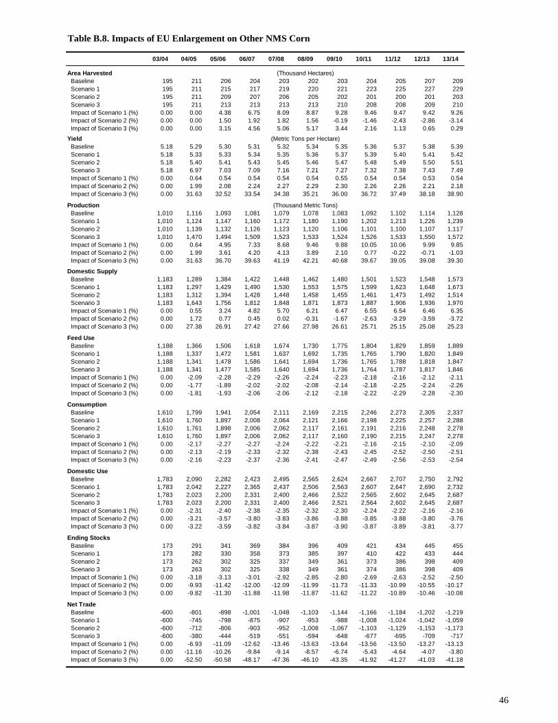
Table B.8. Impacts of EU Enlargement on Other NMS Corn

03/04 04/05 05/06 06/07 07/08 08/09 09/10 10/11 11/12 12/13 13/14

Area Harvested Baseline 195 211 206 204 203 202 203 204 205 207 209 Scenario 1 195 211 215 217 219 220 221 223 225 227 229 Scenario 2 195 211 209 207 206 205 202 201 200 201 203 Scenario 3 195 211 213 213 213 213 210 208 208 209 210 Impact of Scenario 1 (%) 0.00 0.00 4.38 6.75 8.09 8.87 9.28 9.46 9.47 9.42 9.26 Impact of Scenario 2 (%) 0.00 0.00 1.50 1.92 1.82 1.56 -0.19 -1.46 -2.43 -2.86 -3.14 Impact of Scenario 3 (%) 0.00 0.00 3.15 4.56 5.06 5.17 3.44 2.16 1.13 0.65 0.29


Production Baseline 1,010 1,116 1,093 1,081 1,079 1,078 1,083 1,092 1,102 1,114 1,128 Scenario 1 1,010 1,124 1,147 1,160 1,172 1,180 1,190 1,202 1,213 1,226 1,239 Scenario 2 1,010 1,139 1,132 1,126 1,123 1,120 1,106 1,101 1,100 1,107 1,117 Scenario 3 1,010 1,470 1,494 1,509 1,523 1,533 1,524 1,526 1,533 1,550 1,572 Impact of Scenario 1 (%) 0.00 0.64 4.95 7.33 8.68 9.46 9.88 10.05 10.06 9.99 9.85 Impact of Scenario 2 (%) 0.00 1.99 3.61 4.20 4.13 3.89 2.10 0.77 -0.22 -0.71 -1.03 Impact of Scenario 3 (%) 0.00 31.63 36.70 39.63 41.19 42.21 40.68 39.67 39.05 39.08 39.30

Domestic Supply Baseline 1,183 1,289 1,384 1,422 1,448 1,462 1,480 1,501 1,523 1,548 1,573 Scenario 1 1,183 1,297 1,429 1,490 1,530 1,553 1,575 1,599 1,623 1,648 1,673 Scenario 2 1,183 1,312 1,394 1,428 1,448 1,458 1,455 1,461 1,473 1,492 1,514 Scenario 3 1,183 1,643 1,756 1,812 1,848 1,871 1,873 1,887 1,906 1,936 1,970 Impact of Scenario 1 (%) 0.00 0.55 3.24 4.82 5.70 6.21 6.47 6.55 6.54 6.46 6.35 Impact of Scenario 2 (%) 0.00 1.72 0.77 0.45 0.02 -0.31 -1.67 -2.63 -3.29 -3.59 -3.72 Impact of Scenario 3 (%) 0.00 27.38 26.91 27.42 27.66 27.98 26.61 25.71 25.15 25.08 25.23

Feed Use Baseline 1,188 1,366 1,506 1,618 1,674 1,730 1,775 1,804 1,829 1,859 1,889 Scenario 1 1,188 1,337 1,472 1,581 1,637 1,692 1,735 1,765 1,790 1,820 1,849 Scenario 2 1,188 1,341 1,478 1,586 1,641 1,694 1,736 1,765 1,788 1,818 1,847 Scenario 3 1,188 1,341 1,477 1,585 1,640 1,694 1,736 1,764 1,787 1,817 1,846 Impact of Scenario 1 (%) 0.00 -2.09 -2.28 -2.29 -2.26 -2.24 -2.23 -2.18 -2.16 -2.12 -2.11 Impact of Scenario 2 (%) 0.00 -1.77 -1.89 -2.02 -2.02 -2.08 -2.14 -2.18 -2.25 -2.24 -2.26 Impact of Scenario 3 (%) 0.00 -1.81 -1.93 -2.06 -2.06 -2.12 -2.18 -2.22 -2.29 -2.28 -2.30


Domestic Use Baseline 1,783 2,090 2,282 2,423 2,495 2,565 2,624 2,667 2,707 2,750 2,792 Scenario 1 1,783 2,042 2,227 2,365 2,437 2,506 2,563 2,607 2,647 2,690 2,732 Scenario 2 1,783 2,023 2,200 2,331 2,400 2,466 2,522 2,565 2,602 2,645 2,687 Scenario 3 1,783 2,023 2,200 2,331 2,400 2,466 2,521 2,564 2,602 2,645 2,687 Impact of Scenario 1 (%) 0.00 -2.31 -2.40 -2.38 -2.35 -2.32 -2.30 -2.24 -2.22 -2.16 -2.16 Impact of Scenario 2 (%) 0.00 -3.21 -3.57 -3.80 -3.83 -3.86 -3.88 -3.85 -3.88 -3.80 -3.76 Impact of Scenario 3 (%) 0.00 -3.22 -3.59 -3.82 -3.84 -3.87 -3.90 -3.87 -3.89 -3.81 -3.77


Net Trade Baseline -600 -801 -898 -1,001 -1,048 -1,103 -1,144 -1,166 -1,184 -1,202 -1,219 Scenario 1 -600 -745 -798 -875 -907 -953 -988 -1,008 -1,024 -1,042 -1,059 Scenario 2 -600 -712 -806 -903 -952 -1,008 -1,067 -1,103 -1,129 -1,153 -1,173 Scenario 3 -600 -380 -444 -519 -551 -594 -648 -677 -695 -709 -717 Impact of Scenario 1 (%) 0.00 -6.93 -11.09 -12.62 -13.46 -13.63 -13.64 -13.56 -13.50 -13.27 -13.13 Impact of Scenario 2 (%) 0.00 -11.16 -10.26 -9.84 -9.14 -8.57 -6.74 -5.43 -4.64 -4.07 -3.80 Impact of Scenario 3 (%) 0.00 -52.50 -50.58 -48.17 -47.36 -46.10 -43.35 -41.92 -41.27 -41.03 -41.18

(Thousand Hectares)



46

Table B.9. Impacts of EU Enlargement on Other NMS Barley

03/04 04/05 05/06 06/07 07/08 08/09 09/10 10/11 11/12 12/13 13/14

Area Harvested Baseline 937 920 971 970 994 1,001 1,005 1,005 1,004 1,003 1,001 Scenario 1 937 920 942 931 949 955 958 958 957 957 955 Scenario 2 937 920 1,080 1,156 1,220 1,256 1,217 1,201 1,196 1,188 1,179 Scenario 3 937 920 1,181 1,310 1,401 1,451 1,407 1,386 1,377 1,364 1,350 Impact of Scenario 1 (%) 0.00 0.00 -3.01 -4.00 -4.46 -4.61 -4.69 -4.69 -4.64 -4.60 -4.54 Impact of Scenario 2 (%) 0.00 0.00 11.20 19.15 22.76 25.51 21.15 19.53 19.20 18.51 17.85 Impact of Scenario 3 (%) 0.00 0.00 21.66 35.06 41.02 44.97 40.06 37.97 37.19 36.04 34.94








Net Trade Baseline -470 -542 -667 -807 -831 -879 -924 -952 -972 -1,005 -1,049 Scenario 1 -470 -623 -802 -962 -993 -1,044 -1,088 -1,115 -1,133 -1,165 -1,204 Scenario 2 -470 -282 -68 -39 51 65 -99 -180 -224 -282 -341 Scenario 3 -470 697 1,463 1,778 2,049 2,161 1,942 1,831 1,768 1,688 1,606 Impact of Scenario 1 (%) 0.00 14.96 20.28 19.24 19.47 18.77 17.84 17.13 16.60 15.88 14.74 Impact of Scenario 2 (%) 0.00 -48.01 -89.88 -95.16 -106.13 -107.39 -89.23 -81.09 -76.94 -71.92 -67.47 Impact of Scenario 3 (%) 0.00 -228.59 -319.28 -320.34 -346.60 -345.86 -310.27 -292.42 -281.93 -267.90 -253.04

(Thousand Hectares)



47

Table B.10. Impacts of EU Enlargement on Poland Wheat

03/04 04/05 05/06 06/07 07/08 08/09 09/10 10/11 11/12 12/13 13/14

Area Harvested Baseline 2,450 2,470 2,706 2,667 2,624 2,613 2,602 2,592 2,582 2,569 2,560 Scenario 1 2,450 2,470 2,624 2,593 2,555 2,546 2,537 2,527 2,520 2,509 2,502 Scenario 2 2,450 2,470 2,598 2,583 2,575 2,572 2,447 2,446 2,444 2,431 2,423 Scenario 3 2,450 2,470 2,738 2,714 2,699 2,691 2,555 2,549 2,542 2,524 2,511 Impact of Scenario 1 (%) 0.00 0.00 -3.03 -2.80 -2.63 -2.58 -2.53 -2.48 -2.39 -2.33 -2.28 Impact of Scenario 2 (%) 0.00 0.00 -3.98 -3.15 -1.86 -1.56 -5.98 -5.62 -5.33 -5.36 -5.36 Impact of Scenario 3 (%) 0.00 0.00 1.19 1.74 2.84 2.97 -1.82 -1.65 -1.54 -1.76 -1.90

Yield Baseline 3.22 3.59 3.60 3.62 3.64 3.66 3.69 3.72 3.74 3.77 3.79 Scenario 1 3.22 3.57 3.57 3.60 3.62 3.65 3.67 3.70 3.72 3.75 3.78 Scenario 2 3.22 3.55 3.56 3.59 3.62 3.65 3.67 3.70 3.72 3.75 3.77 Scenario 3 3.22 4.59 4.61 4.65 4.69 4.72 4.76 4.79 4.83 4.86 4.90 Impact of Scenario 1 (%) 0.00 -0.68 -0.61 -0.55 -0.53 -0.51 -0.49 -0.46 -0.44 -0.42 -0.40 Impact of Scenario 2 (%) 0.00 -1.26 -0.93 -0.65 -0.57 -0.53 -0.50 -0.51 -0.49 -0.47 -0.50 Impact of Scenario 3 (%) 0.00 27.76 28.21 28.55 28.72 28.84 28.91 28.95 29.00 29.08 29.10

Production Baseline 7,900 8,871 9,732 9,646 9,553 9,576 9,602 9,629 9,658 9,675 9,707 Scenario 1 7,900 8,811 9,380 9,324 9,252 9,281 9,313 9,347 9,386 9,409 9,448 Scenario 2 7,900 8,759 9,257 9,281 9,322 9,377 8,983 9,041 9,098 9,113 9,141 Scenario 3 7,900 11,334 12,625 12,616 12,645 12,704 12,153 12,211 12,268 12,269 12,294 Impact of Scenario 1 (%) 0.00 -0.68 -3.61 -3.34 -3.15 -3.08 -3.01 -2.93 -2.82 -2.74 -2.67 Impact of Scenario 2 (%) 0.00 -1.26 -4.88 -3.78 -2.42 -2.08 -6.45 -6.10 -5.80 -5.81 -5.83 Impact of Scenario 3 (%) 0.00 27.76 29.73 30.79 32.37 32.67 26.57 26.82 27.02 26.81 26.65

Domestic Supply Baseline 8,300 9,171 10,021 10,012 9,983 10,038 10,085 10,135 10,187 10,229 10,280 Scenario 1 8,300 9,111 9,746 9,766 9,754 9,812 9,862 9,917 9,975 10,022 10,077 Scenario 2 8,300 9,059 9,690 9,768 9,839 9,913 9,534 9,613 9,693 9,732 9,777 Scenario 3 8,300 11,634 13,063 13,108 13,168 13,246 12,710 12,789 12,867 12,892 12,935 Impact of Scenario 1 (%) 0.00 -0.65 -2.74 -2.45 -2.30 -2.25 -2.21 -2.16 -2.08 -2.03 -1.98 Impact of Scenario 2 (%) 0.00 -1.22 -3.30 -2.44 -1.45 -1.24 -5.46 -5.15 -4.85 -4.86 -4.89 Impact of Scenario 3 (%) 0.00 26.86 30.36 30.93 31.90 31.96 26.03 26.18 26.31 26.04 25.82

Feed Use Baseline 3,200 3,106 2,844 3,136 3,247 3,295 3,330 3,374 3,427 3,496 3,545 Scenario 1 3,200 3,192 2,912 3,205 3,317 3,364 3,399 3,441 3,493 3,561 3,612 Scenario 2 3,200 3,318 3,031 3,311 3,426 3,471 3,505 3,546 3,595 3,662 3,715 Scenario 3 3,200 3,319 3,032 3,312 3,427 3,472 3,506 3,547 3,596 3,663 3,716 Impact of Scenario 1 (%) 0.00 2.77 2.39 2.21 2.16 2.11 2.07 1.99 1.94 1.87 1.87 Impact of Scenario 2 (%) 0.00 6.81 6.55 5.57 5.52 5.34 5.24 5.11 4.92 4.75 4.80 Impact of Scenario 3 (%) 0.00 6.84 6.59 5.60 5.55 5.37 5.28 5.15 4.95 4.78 4.83

Consumption Baseline 8,750 8,519 8,250 8,567 8,699 8,765 8,818 8,876 8,947 9,034 9,098 Scenario 1 8,750 8,737 8,475 8,791 8,920 8,982 9,028 9,079 9,144 9,225 9,286 Scenario 2 8,750 8,998 8,724 8,986 9,094 9,142 9,185 9,240 9,303 9,382 9,454 Scenario 3 8,750 9,007 8,735 8,997 9,106 9,154 9,196 9,250 9,313 9,392 9,463 Impact of Scenario 1 (%) 0.00 2.56 2.72 2.62 2.54 2.47 2.39 2.29 2.20 2.11 2.06 Impact of Scenario 2 (%) 0.00 5.62 5.74 4.89 4.55 4.31 4.17 4.09 3.98 3.86 3.91 Impact of Scenario 3 (%) 0.00 5.73 5.88 5.03 4.68 4.43 4.30 4.21 4.09 3.97 4.02

Domestic Use Baseline 9,050 8,808 8,615 8,998 9,160 9,248 9,324 9,405 9,501 9,607 9,689 Scenario 1 9,050 9,103 8,917 9,293 9,450 9,530 9,599 9,668 9,756 9,854 9,930 Scenario 2 9,050 9,430 9,210 9,503 9,630 9,694 9,758 9,835 9,922 10,018 10,111 Scenario 3 9,050 9,445 9,227 9,520 9,647 9,710 9,774 9,850 9,937 10,033 10,125 Impact of Scenario 1 (%) 0.00 3.35 3.50 3.29 3.16 3.06 2.94 2.80 2.68 2.57 2.49 Impact of Scenario 2 (%) 0.00 7.06 6.90 5.62 5.13 4.82 4.65 4.57 4.42 4.28 4.36 Impact of Scenario 3 (%) 0.00 7.23 7.10 5.81 5.31 5.00 4.82 4.73 4.58 4.43 4.50

Ending Stocks Baseline 300 289 365 431 462 483 507 529 554 573 591 Scenario 1 300 366 442 502 530 549 570 589 612 629 645 Scenario 2 300 432 486 518 536 551 572 595 619 636 657 Scenario 3 300 438 492 523 541 556 577 600 624 641 662 Impact of Scenario 1 (%) 0.00 26.74 21.04 16.54 14.80 13.71 12.55 11.44 10.44 9.74 9.12 Impact of Scenario 2 (%) 0.00 49.71 33.04 20.14 16.03 14.20 13.02 12.52 11.68 11.02 11.23 Impact of Scenario 3 (%) 0.00 51.57 34.57 21.39 17.17 15.26 14.00 13.43 12.50 11.79 11.95

Net Trade Baseline -750 363 1,405 1,014 823 790 761 730 686 622 592 Scenario 1 -750 8 829 473 304 281 264 248 219 168 147 Scenario 2 -750 -371 480 264 209 219 -224 -221 -228 -286 -334 Scenario 3 -750 2,189 3,836 3,588 3,521 3,535 2,936 2,939 2,931 2,860 2,810 Impact of Scenario 1 (%) 0.00 -97.88 -40.99 -53.34 -63.05 -64.41 -65.33 -66.00 -68.01 -73.01 -75.21 Impact of Scenario 2 (%) 0.00 -202.21 -65.87 -73.94 -74.61 -72.24 -129.44 -130.28 -133.31 -146.02 -156.38 Impact of Scenario 3 (%) 0.00 503.27 172.96 253.79 327.87 347.62 285.84 302.57 327.41 359.41 375.02

(Thousand Hectares)



48

Table B.11. Impacts of EU Enlargement on Poland Corn

03/04 04/05 05/06 06/07 07/08 08/09 09/10 10/11 11/12 12/13 13/14

Area Harvested Baseline 350 351 296 292 294 313 313 312 312 311 311 Scenario 1 350 351 301 296 298 317 317 316 315 315 314 Scenario 2 350 351 320 316 317 337 320 321 320 319 318 Scenario 3 350 351 323 319 320 341 324 325 325 324 323 Impact of Scenario 1 (%) 0.00 0.00 1.70 1.38 1.32 1.22 1.22 1.23 1.19 1.20 1.16 Impact of Scenario 2 (%) 0.00 0.00 8.17 7.94 7.93 7.50 2.40 2.60 2.70 2.56 2.38 Impact of Scenario 3 (%) 0.00 0.00 9.21 9.03 9.11 8.72 3.67 3.96 4.12 4.04 3.93


Production Baseline 1,900 2,130 1,812 1,809 1,836 1,979 1,997 2,014 2,030 2,047 2,065 Scenario 1 1,900 2,137 1,847 1,839 1,864 2,008 2,027 2,044 2,060 2,076 2,095 Scenario 2 1,900 2,168 1,995 1,990 2,018 2,167 2,083 2,103 2,121 2,134 2,148 Scenario 3 1,900 2,486 2,320 2,328 2,378 2,569 2,486 2,525 2,562 2,593 2,625 Impact of Scenario 1 (%) 0.00 0.35 1.95 1.62 1.57 1.47 1.48 1.48 1.44 1.43 1.41 Impact of Scenario 2 (%) 0.00 1.81 10.11 9.98 9.95 9.51 4.28 4.41 4.47 4.25 4.01 Impact of Scenario 3 (%) 0.00 16.73 28.06 28.67 29.53 29.83 24.45 25.37 26.17 26.66 27.10

Domestic Supply Baseline 2,478 2,628 2,272 2,250 2,266 2,405 2,421 2,438 2,456 2,475 2,496 Scenario 1 2,478 2,635 2,305 2,276 2,291 2,429 2,445 2,462 2,480 2,499 2,520 Scenario 2 2,478 2,666 2,442 2,408 2,420 2,560 2,470 2,489 2,508 2,523 2,540 Scenario 3 2,478 2,984 2,767 2,747 2,780 2,962 2,873 2,911 2,948 2,982 3,017 Impact of Scenario 1 (%) 0.00 0.28 1.44 1.15 1.08 1.01 1.02 1.01 0.98 0.97 0.95 Impact of Scenario 2 (%) 0.00 1.47 7.47 7.03 6.78 6.44 2.03 2.08 2.11 1.93 1.76 Impact of Scenario 3 (%) 0.00 13.56 21.79 22.07 22.65 23.18 18.69 19.42 20.07 20.48 20.88

Feed Use Baseline 1,900 1,936 1,805 1,992 2,071 2,106 2,134 2,169 2,208 2,256 2,295 Scenario 1 1,900 1,925 1,795 1,981 2,060 2,094 2,122 2,157 2,196 2,244 2,283 Scenario 2 1,900 1,884 1,747 1,923 1,999 2,031 2,059 2,094 2,133 2,182 2,222 Scenario 3 1,900 1,884 1,747 1,924 1,999 2,032 2,059 2,095 2,133 2,182 2,222 Impact of Scenario 1 (%) 0.00 -0.56 -0.54 -0.54 -0.53 -0.53 -0.54 -0.52 -0.53 -0.51 -0.52 Impact of Scenario 2 (%) 0.00 -2.68 -3.20 -3.46 -3.50 -3.52 -3.51 -3.43 -3.38 -3.29 -3.20 Impact of Scenario 3 (%) 0.00 -2.66 -3.18 -3.44 -3.48 -3.50 -3.49 -3.41 -3.36 -3.27 -3.18


Domestic Use Baseline 2,498 2,506 2,356 2,534 2,608 2,640 2,668 2,704 2,746 2,797 2,838 Scenario 1 2,498 2,491 2,342 2,518 2,591 2,622 2,650 2,686 2,727 2,778 2,819 Scenario 2 2,498 2,434 2,269 2,429 2,495 2,522 2,548 2,584 2,625 2,676 2,720 Scenario 3 2,498 2,434 2,270 2,430 2,496 2,523 2,549 2,585 2,626 2,677 2,720 Impact of Scenario 1 (%) 0.00 -0.60 -0.63 -0.65 -0.65 -0.66 -0.68 -0.67 -0.67 -0.66 -0.66 Impact of Scenario 2 (%) 0.00 -2.89 -3.70 -4.15 -4.33 -4.46 -4.50 -4.45 -4.40 -4.30 -4.18 Impact of Scenario 3 (%) 0.00 -2.87 -3.67 -4.13 -4.30 -4.43 -4.47 -4.42 -4.37 -4.27 -4.16


Net Trade Baseline -20 122 -84 -284 -341 -235 -247 -266 -290 -322 -342 Scenario 1 -20 144 -36 -242 -300 -193 -205 -224 -248 -279 -299 Scenario 2 -20 232 173 -21 -75 37 -78 -95 -117 -153 -179 Scenario 3 -20 550 498 317 284 439 325 327 323 305 297 Impact of Scenario 1 (%) 0.00 18.47 -56.70 -14.87 -12.16 -17.84 -17.29 -16.01 -14.64 -13.15 -12.43 Impact of Scenario 2 (%) 0.00 91.13 -305.63 -92.67 -78.14 -115.95 -68.50 -64.24 -59.52 -52.27 -47.53 Impact of Scenario 3 (%) 0.00 352.00 -692.01 -211.56 -183.34 -286.92 -231.25 -222.54 -211.23 -194.79 -186.86

(Thousand Hectares)



49

Table B.12. Impacts of EU Enlargement on Poland Barley

03/04 04/05 05/06 06/07 07/08 08/09 09/10 10/11 11/12 12/13 13/14

Area Harvested Baseline 1,000 972 1,051 1,044 1,041 1,035 1,034 1,032 1,030 1,028 1,026 Scenario 1 1,000 972 1,035 1,031 1,029 1,023 1,023 1,021 1,019 1,017 1,016 Scenario 2 1,000 972 1,060 1,074 1,075 1,077 1,029 1,023 1,025 1,019 1,015 Scenario 3 1,000 972 1,077 1,093 1,095 1,097 1,049 1,043 1,045 1,039 1,035 Impact of Scenario 1 (%) 0.00 0.00 -1.50 -1.27 -1.21 -1.14 -1.13 -1.10 -1.05 -1.02 -0.99 Impact of Scenario 2 (%) 0.00 0.00 0.83 2.83 3.23 3.99 -0.56 -0.87 -0.53 -0.88 -1.15 Impact of Scenario 3 (%) 0.00 0.00 2.45 4.69 5.14 5.97 1.38 1.08 1.44 1.07 0.84

Yield Baseline 2.80 3.14 3.17 3.21 3.25 3.30 3.34 3.39 3.43 3.48 3.52 Scenario 1 2.80 3.12 3.16 3.20 3.24 3.29 3.33 3.38 3.42 3.47 3.51 Scenario 2 2.80 3.11 3.16 3.20 3.25 3.29 3.34 3.38 3.42 3.47 3.51 Scenario 3 2.80 3.59 3.66 3.72 3.79 3.87 3.94 4.01 4.07 4.15 4.22 Impact of Scenario 1 (%) 0.00 -0.37 -0.31 -0.29 -0.26 -0.25 -0.23 -0.21 -0.20 -0.18 -0.16 Impact of Scenario 2 (%) 0.00 -0.97 -0.22 -0.23 -0.05 -0.08 -0.09 -0.12 -0.18 -0.20 -0.18 Impact of Scenario 3 (%) 0.00 14.34 15.37 15.84 16.68 17.30 17.84 18.32 18.74 19.29 19.81

Production Baseline 2,800 3,048 3,331 3,352 3,386 3,413 3,456 3,494 3,534 3,573 3,613 Scenario 1 2,800 3,036 3,270 3,300 3,336 3,366 3,409 3,449 3,490 3,530 3,572 Scenario 2 2,800 3,018 3,351 3,439 3,494 3,547 3,434 3,460 3,509 3,535 3,565 Scenario 3 2,800 3,485 3,936 4,065 4,154 4,243 4,129 4,179 4,256 4,308 4,365 Impact of Scenario 1 (%) 0.00 -0.37 -1.81 -1.56 -1.47 -1.39 -1.36 -1.31 -1.24 -1.21 -1.15 Impact of Scenario 2 (%) 0.00 -0.97 0.61 2.59 3.17 3.91 -0.65 -0.99 -0.71 -1.08 -1.33 Impact of Scenario 3 (%) 0.00 14.34 18.19 21.28 22.68 24.31 19.47 19.60 20.44 20.57 20.81

Domestic Supply Baseline 2,985 3,083 3,372 3,410 3,453 3,488 3,535 3,578 3,622 3,666 3,709 Scenario 1 2,985 3,071 3,315 3,362 3,409 3,445 3,493 3,537 3,582 3,626 3,671 Scenario 2 2,985 3,053 3,402 3,503 3,566 3,624 3,515 3,545 3,599 3,630 3,664 Scenario 3 2,985 3,520 3,989 4,130 4,227 4,321 4,211 4,266 4,347 4,405 4,465 Impact of Scenario 1 (%) 0.00 -0.37 -1.67 -1.40 -1.29 -1.23 -1.20 -1.16 -1.10 -1.07 -1.02 Impact of Scenario 2 (%) 0.00 -0.96 0.91 2.72 3.25 3.89 -0.58 -0.92 -0.63 -0.98 -1.21 Impact of Scenario 3 (%) 0.00 14.17 18.30 21.13 22.41 23.88 19.11 19.21 20.03 20.15 20.39

Feed Use Baseline 2,600 2,442 2,238 2,441 2,529 2,563 2,590 2,625 2,663 2,715 2,758 Scenario 1 2,600 2,440 2,235 2,438 2,526 2,559 2,586 2,621 2,659 2,711 2,753 Scenario 2 2,600 2,449 2,225 2,432 2,514 2,549 2,577 2,614 2,655 2,709 2,751 Scenario 3 2,600 2,451 2,227 2,434 2,516 2,551 2,579 2,616 2,657 2,711 2,753 Impact of Scenario 1 (%) 0.00 -0.10 -0.14 -0.12 -0.14 -0.14 -0.14 -0.15 -0.15 -0.16 -0.18 Impact of Scenario 2 (%) 0.00 0.27 -0.57 -0.40 -0.59 -0.53 -0.49 -0.42 -0.29 -0.22 -0.25 Impact of Scenario 3 (%) 0.00 0.35 -0.48 -0.31 -0.50 -0.45 -0.41 -0.35 -0.22 -0.14 -0.18

Consumption Baseline 3,300 3,029 2,832 3,048 3,154 3,202 3,244 3,293 3,346 3,412 3,471 Scenario 1 3,300 3,045 2,851 3,067 3,172 3,220 3,261 3,309 3,361 3,426 3,483 Scenario 2 3,300 3,097 2,879 3,100 3,195 3,244 3,286 3,338 3,396 3,464 3,521 Scenario 3 3,300 3,101 2,884 3,105 3,201 3,249 3,292 3,342 3,400 3,469 3,526 Impact of Scenario 1 (%) 0.00 0.51 0.65 0.64 0.58 0.56 0.52 0.47 0.44 0.41 0.35 Impact of Scenario 2 (%) 0.00 2.24 1.67 1.71 1.31 1.31 1.31 1.35 1.49 1.53 1.44 Impact of Scenario 3 (%) 0.00 2.38 1.84 1.88 1.48 1.48 1.47 1.50 1.63 1.67 1.57

Domestic Use Baseline 3,335 3,070 2,890 3,115 3,229 3,282 3,328 3,381 3,438 3,508 3,571 Scenario 1 3,335 3,090 2,913 3,139 3,252 3,304 3,349 3,401 3,457 3,525 3,587 Scenario 2 3,335 3,148 2,943 3,172 3,273 3,325 3,372 3,428 3,491 3,563 3,625 Scenario 3 3,335 3,153 2,949 3,178 3,279 3,332 3,378 3,434 3,497 3,569 3,630 Impact of Scenario 1 (%) 0.00 0.64 0.80 0.78 0.71 0.68 0.64 0.58 0.54 0.50 0.43 Impact of Scenario 2 (%) 0.00 2.55 1.85 1.82 1.35 1.34 1.33 1.37 1.53 1.58 1.50 Impact of Scenario 3 (%) 0.00 2.71 2.05 2.03 1.55 1.53 1.51 1.55 1.70 1.74 1.65

Ending Stocks Baseline 35 41 58 67 75 80 84 88 92 96 100 Scenario 1 35 45 62 72 80 84 88 92 96 99 103 Scenario 2 35 51 64 72 77 81 86 90 95 99 103 Scenario 3 35 52 65 73 79 82 87 91 96 100 104 Impact of Scenario 1 (%) 0.00 9.65 8.32 7.32 6.24 5.68 5.08 4.47 4.01 3.66 3.17 Impact of Scenario 2 (%) 0.00 25.19 10.54 7.06 3.03 2.21 1.92 2.25 3.05 3.50 3.41 Impact of Scenario 3 (%) 0.00 27.20 12.40 8.73 4.53 3.61 3.20 3.44 4.14 4.52 4.36

Net Trade Baseline -350 13 482 295 224 207 207 197 184 158 138 Scenario 1 -350 -18 402 223 157 142 144 136 125 101 85 Scenario 2 -350 -95 459 331 293 299 143 118 108 67 40 Scenario 3 -350 366 1,040 952 948 990 833 832 851 836 835 Impact of Scenario 1 (%) 0.00 -245.17 -16.51 -24.37 -30.15 -31.50 -30.68 -30.98 -31.80 -35.92 -38.73 Impact of Scenario 2 (%) 0.00 -857.47 -4.70 12.23 30.58 44.39 -31.18 -40.33 -41.11 -57.73 -71.27 Impact of Scenario 3 (%) 0.00 2,811.91 115.76 222.91 322.84 378.64 301.57 322.33 363.19 428.54 505.47

(Thousand Hectares)



50

Table B.13. Impacts of EU Enlargement on Grain Prices

03/04 04/05 05/06 06/07 07/08 08/09 09/10 10/11 11/12 12/13 13/14

European Union 25Wheat Domestic Price Baseline 120 118 120 117 117 117 115 113 112 111 110 Scenario 1 120 118 120 117 117 117 115 113 112 112 111 Scenario 2 120 118 120 117 117 116 115 113 112 111 110 Scenario 3 120 117 119 117 116 116 115 112 111 111 110 Impact of Scenario 1 (%) 0.00 0.13 0.15 0.06 0.05 0.09 0.10 0.08 0.08 0.09 0.09 Impact of Scenario 2 (%) 0.00 -0.04 -0.16 -0.17 -0.14 -0.14 0.05 -0.03 -0.13 -0.08 -0.06 Impact of Scenario 3 (%) 0.00 -0.83 -0.93 -0.58 -0.60 -0.81 -0.57 -0.62 -0.77 -0.76 -0.71

Corn Domestic Price Baseline 139 124 130 128 127 126 123 123 121 121 118 Scenario 1 139 124 130 128 127 126 123 123 121 121 118 Scenario 2 139 124 130 128 127 126 123 123 121 121 118 Scenario 3 139 123 130 128 127 125 123 123 121 121 118 Impact of Scenario 1 (%) 0.00 0.03 0.05 0.04 0.03 0.02 0.03 0.04 0.03 0.03 0.03 Impact of Scenario 2 (%) 0.00 -0.02 -0.07 -0.08 -0.08 -0.07 -0.01 -0.02 -0.04 -0.09 -0.08 Impact of Scenario 3 (%) 0.00 -0.24 -0.33 -0.33 -0.28 -0.27 -0.25 -0.30 -0.29 -0.29 -0.33

Barley Domestic Price Baseline 113 112 115 112 111 111 109 108 107 106 104 Scenario 1 113 112 115 112 111 111 109 108 107 106 104 Scenario 2 113 112 114 112 111 110 109 107 107 106 104 Scenario 3 113 111 113 111 110 109 108 107 106 105 103 Impact of Scenario 1 (%) 0.00 0.12 0.14 0.08 0.07 0.09 0.10 0.10 0.09 0.09 0.10 Impact of Scenario 2 (%) 0.00 -0.09 -0.28 -0.28 -0.26 -0.27 -0.03 -0.13 -0.20 -0.21 -0.17 Impact of Scenario 3 (%) 0.00 -0.99 -1.09 -0.90 -0.88 -1.07 -0.79 -0.92 -1.02 -1.04 -1.04

WorldWheat U.S. FOB Gulf Baseline 145 141 140 138 139 141 142 144 145 146 149 Scenario 1 145 142 142 140 141 142 143 145 146 148 150 Scenario 2 145 141 139 137 137 139 142 143 144 146 148 Scenario 3 145 133 130 128 129 130 133 134 135 136 138 Impact of Scenario 1 (%) 0.00 0.89 1.16 0.99 0.98 0.98 0.94 0.92 0.90 0.89 0.87 Impact of Scenario 2 (%) 0.00 -0.17 -0.85 -1.26 -1.41 -1.47 -0.19 -0.46 -0.52 -0.39 -0.32 Impact of Scenario 3 (%) 0.00 -5.30 -6.88 -7.09 -7.68 -7.85 -6.34 -6.75 -6.98 -6.92 -6.96

Corn U.S. FOB Gulf Baseline 104 106 106 105 107 107 107 108 108 109 110 Scenario 1 104 106 106 105 107 107 107 108 108 109 110 Scenario 2 104 105 105 104 105 106 107 107 107 108 109 Scenario 3 104 101 102 100 102 102 103 102 103 103 104 Impact of Scenario 1 (%) 0.00 0.09 0.10 0.09 0.05 0.06 0.03 0.04 0.02 0.03 0.01 Impact of Scenario 2 (%) 0.00 -0.67 -0.88 -1.06 -1.11 -1.19 -0.57 -0.92 -0.67 -0.87 -0.62 Impact of Scenario 3 (%) 0.00 -4.40 -3.11 -4.82 -4.10 -5.17 -3.85 -4.98 -4.36 -5.15 -4.64

Barley Canada Feed Baseline 92 89 85 88 88 89 90 91 93 94 95 Scenario 1 92 90 87 89 89 90 91 93 94 95 96 Scenario 2 92 88 82 84 84 85 88 89 91 92 93 Scenario 3 92 79 74 75 73 74 78 78 79 80 81 Impact of Scenario 1 (%) 0.00 1.26 1.68 1.42 1.50 1.47 1.44 1.40 1.38 1.37 1.32 Impact of Scenario 2 (%) 0.00 -1.07 -3.75 -3.81 -4.67 -4.77 -1.96 -3.02 -2.52 -2.49 -2.33 Impact of Scenario 3 (%) 0.00 -11.22 -13.31 -15.05 -16.15 -17.11 -13.41 -15.15 -14.58 -14.91 -14.91

(Euro per Metric Ton)

(U.S. Dollars per Metric Ton)

51

Table B.13. Impacts of EU Enlargement on Grain Prices (continued)

03/04 04/05 05/06 06/07 07/08 08/09 09/10 10/11 11/12 12/13 13/14

Czech RepublicWheat Domestic Price Baseline 5,040 6,168 5,721 5,366 5,142 4,921 4,748 4,779 4,789 4,794 4,828 Scenario 1 5,040 5,658 5,253 4,929 4,724 4,522 4,366 4,402 4,413 4,420 4,455 Scenario 2 5,040 7,782 7,489 7,300 7,072 6,796 6,557 6,571 6,574 6,578 6,559 Scenario 3 5,040 7,722 7,431 7,243 7,017 6,744 6,506 6,520 6,523 6,527 6,508 Impact of Scenario 1 (%) 0.00 -8.27 -8.18 -8.15 -8.15 -8.11 -8.05 -7.89 -7.85 -7.80 -7.73 Impact of Scenario 2 (%) 0.00 26.17 30.91 36.03 37.52 38.10 38.09 37.49 37.27 37.21 35.85 Impact of Scenario 3 (%) 0.00 25.19 29.90 34.97 36.45 37.03 37.02 36.42 36.21 36.15 34.80

Corn Domestic Price Baseline 3,477 2,641 2,467 2,340 2,248 2,144 2,057 2,050 2,041 2,039 2,036 Scenario 1 3,477 2,842 2,627 2,500 2,404 2,298 2,212 2,206 2,205 2,201 2,208 Scenario 2 3,477 3,398 3,240 3,163 3,068 2,954 2,858 2,859 2,870 2,868 2,872 Scenario 3 3,477 3,389 3,232 3,154 3,060 2,946 2,850 2,852 2,863 2,861 2,864 Impact of Scenario 1 (%) 0.00 7.61 6.48 6.82 6.93 7.18 7.57 7.61 8.02 7.96 8.48 Impact of Scenario 2 (%) 0.00 28.65 31.34 35.16 36.47 37.75 38.97 39.48 40.65 40.67 41.08 Impact of Scenario 3 (%) 0.00 28.30 30.99 34.80 36.10 37.38 38.60 39.10 40.27 40.29 40.70

Barley Domestic Price Baseline 3,208 6,486 5,797 5,675 5,386 5,200 5,023 5,063 5,115 5,139 5,131 Scenario 1 3,208 6,196 5,542 5,428 5,159 4,983 4,820 4,867 4,920 4,947 4,952 Scenario 2 3,208 6,889 6,618 6,458 6,260 6,018 5,809 5,822 5,827 5,832 5,827 Scenario 3 3,208 6,833 6,564 6,406 6,209 5,969 5,762 5,775 5,779 5,784 5,779 Impact of Scenario 1 (%) 0.00 -4.48 -4.40 -4.35 -4.21 -4.17 -4.05 -3.88 -3.81 -3.74 -3.50 Impact of Scenario 2 (%) 0.00 6.21 14.16 13.79 16.23 15.73 15.64 14.99 13.91 13.48 13.55 Impact of Scenario 3 (%) 0.00 5.35 13.23 12.87 15.29 14.79 14.70 14.06 12.98 12.56 12.63

Hungary Wheat Domestic Price Baseline 43,282 39,824 37,387 35,731 35,484 35,632 34,152 34,373 34,444 34,485 34,863 Scenario 1 43,282 33,541 31,521 30,135 29,927 30,065 28,835 29,072 29,143 29,194 29,535 Scenario 2 43,282 50,498 49,190 48,850 49,044 49,456 47,399 47,497 47,520 47,556 47,600 Scenario 3 43,282 50,106 48,809 48,471 48,663 49,072 47,032 47,128 47,152 47,187 47,231 Impact of Scenario 1 (%) 0.00 -15.78 -15.69 -15.66 -15.66 -15.63 -15.57 -15.42 -15.39 -15.34 -15.28 Impact of Scenario 2 (%) 0.00 26.80 31.57 36.71 38.21 38.79 38.79 38.18 37.96 37.90 36.53 Impact of Scenario 3 (%) 0.00 25.82 30.55 35.65 37.14 37.72 37.71 37.11 36.89 36.83 35.48

Corn Domestic Price Baseline 30,927 23,849 22,549 21,789 21,695 21,712 20,686 20,619 20,528 20,512 20,556 Scenario 1 30,927 22,748 21,281 20,630 20,563 20,628 19,723 19,667 19,655 19,628 19,766 Scenario 2 30,927 31,378 30,289 30,120 30,279 30,588 29,401 29,412 29,529 29,510 29,660 Scenario 3 30,927 31,294 30,208 30,039 30,198 30,506 29,322 29,333 29,450 29,431 29,581 Impact of Scenario 1 (%) 0.00 -4.62 -5.62 -5.32 -5.22 -5.00 -4.65 -4.62 -4.25 -4.31 -3.84 Impact of Scenario 2 (%) 0.00 31.57 34.33 38.23 39.57 40.88 42.13 42.64 43.85 43.86 44.29 Impact of Scenario 3 (%) 0.00 31.22 33.97 37.86 39.19 40.50 41.75 42.26 43.46 43.48 43.90

Barley Domestic Price Baseline 27,714 49,296 44,597 44,482 43,746 44,315 42,527 42,864 43,307 43,512 43,614 Scenario 1 27,714 42,973 38,910 38,829 38,246 38,756 37,239 37,601 38,017 38,225 38,410 Scenario 2 27,714 55,134 53,611 53,302 53,545 54,008 51,787 51,904 51,947 51,996 52,150 Scenario 3 27,714 54,688 53,177 52,870 53,111 53,570 51,367 51,483 51,527 51,575 51,728 Impact of Scenario 1 (%) 0.00 -12.83 -12.75 -12.71 -12.57 -12.54 -12.44 -12.28 -12.22 -12.15 -11.93 Impact of Scenario 2 (%) 0.00 11.84 20.21 19.83 22.40 21.87 21.77 21.09 19.95 19.50 19.57 Impact of Scenario 3 (%) 0.00 10.94 19.24 18.86 21.41 20.88 20.79 20.11 18.98 18.53 18.60

(Koruny per Metric Ton)

(Florint per Metric Ton)

52

Table B.13. Impacts of EU Enlargement on Grain Prices (continued)

03/04 04/05 05/06 06/07 07/08 08/09 09/10 10/11 11/12 12/13 13/14

Other NMSWheat Domestic Price Baseline 191 214 212 210 211 213 215 218 220 222 225 Scenario 1 191 180 179 177 179 180 182 185 186 188 191 Scenario 2 191 236 243 250 254 258 260 262 264 267 268 Scenario 3 191 234 241 248 252 256 258 260 262 265 266 Impact of Scenario 1 (%) 0.00 -15.63 -15.54 -15.51 -15.51 -15.48 -15.42 -15.27 -15.24 -15.19 -15.13 Impact of Scenario 2 (%) 0.00 10.46 14.61 19.09 20.40 20.91 20.90 20.37 20.18 20.13 18.94 Impact of Scenario 3 (%) 0.00 9.60 13.73 18.17 19.47 19.97 19.96 19.44 19.25 19.20 18.01

Corn Domestic Price Baseline 118 97 97 96 97 98 98 99 99 100 100 Scenario 1 118 106 105 105 107 107 108 109 109 110 111 Scenario 2 118 127 130 133 136 138 140 141 142 143 145 Scenario 3 118 127 129 133 136 138 139 140 142 143 144 Impact of Scenario 1 (%) 0.00 10.13 8.97 9.31 9.43 9.69 10.08 10.13 10.55 10.48 11.02 Impact of Scenario 2 (%) 0.00 31.65 34.41 38.32 39.65 40.96 42.22 42.73 43.93 43.95 44.38 Impact of Scenario 3 (%) 0.00 31.30 34.05 37.95 39.28 40.59 41.84 42.35 43.55 43.57 43.99

Barley Domestic Price Baseline 123 166 159 163 163 166 168 170 173 175 176 Scenario 1 123 144 138 142 142 145 147 149 152 154 155 Scenario 2 123 211 217 223 227 230 232 235 236 238 240 Scenario 3 123 209 215 221 225 228 230 233 235 237 238 Impact of Scenario 1 (%) 0.00 -12.98 -12.91 -12.86 -12.73 -12.70 -12.59 -12.44 -12.37 -12.31 -12.09 Impact of Scenario 2 (%) 0.00 27.23 36.75 36.31 39.24 38.64 38.53 37.75 36.45 35.94 36.02 Impact of Scenario 3 (%) 0.00 26.20 35.64 35.21 38.11 37.51 37.40 36.63 35.35 34.84 34.92

PolandWheat Domestic Price Baseline 694 708 658 622 612 610 610 614 615 621 625 Scenario 1 694 643 598 565 556 554 555 560 561 566 571 Scenario 2 694 586 565 555 552 553 553 554 554 559 557 Scenario 3 694 582 561 551 548 548 549 550 550 555 553 Impact of Scenario 1 (%) 0.00 -9.24 -9.15 -9.12 -9.12 -9.08 -9.02 -8.86 -8.83 -8.78 -8.71 Impact of Scenario 2 (%) 0.00 -17.19 -14.08 -10.72 -9.74 -9.36 -9.36 -9.76 -9.90 -9.94 -10.83 Impact of Scenario 3 (%) 0.00 -17.83 -14.74 -11.41 -10.44 -10.06 -10.07 -10.46 -10.60 -10.64 -11.53

Corn Domestic Price Baseline 486 378 353 338 333 331 329 328 327 329 328 Scenario 1 486 396 367 352 347 346 345 344 344 346 347 Scenario 2 486 474 453 445 443 444 446 446 448 451 452 Scenario 3 486 472 451 444 442 443 445 445 447 450 450 Impact of Scenario 1 (%) 0.00 4.92 3.82 4.15 4.26 4.50 4.88 4.92 5.32 5.26 5.77 Impact of Scenario 2 (%) 0.00 25.43 28.06 31.78 33.05 34.30 35.50 35.99 37.13 37.15 37.56 Impact of Scenario 3 (%) 0.00 25.10 27.72 31.43 32.70 33.94 35.13 35.62 36.77 36.78 37.19

Barley Domestic Price Baseline 433 577 517 510 496 499 500 504 509 516 515 Scenario 1 433 557 499 492 480 483 485 489 495 501 502 Scenario 2 433 524 504 496 493 494 494 495 496 500 500 Scenario 3 433 520 500 492 489 490 490 491 492 496 496 Impact of Scenario 1 (%) 0.00 -3.53 -3.45 -3.40 -3.25 -3.22 -3.09 -2.92 -2.85 -2.78 -2.54 Impact of Scenario 2 (%) 0.00 -9.21 -2.41 -2.73 -0.64 -1.07 -1.15 -1.70 -2.63 -2.99 -2.93 Impact of Scenario 3 (%) 0.00 -9.94 -3.20 -3.51 -1.44 -1.87 -1.95 -2.50 -3.41 -3.78 -3.72

(U.S. Dollars per Metric Ton)

(Zlotys per Metric Ton)

53

Table B.14. Impacts of EU Enlargement on Grain Production

03/04 04/05 05/06 06/07 07/08 08/09 09/10 10/11 11/12 12/13 13/14

European Union 15Wheat Production Baseline 91,000 102,791 101,305 103,205 103,614 104,791 105,637 106,153 106,642 107,066 107,553 Scenario 1 91,000 102,799 101,325 103,237 103,643 104,812 105,658 106,178 106,667 107,089 107,575 Scenario 2 91,000 102,788 101,293 103,176 103,572 104,748 105,609 106,136 106,638 107,050 107,527 Scenario 3 91,000 102,738 101,179 102,987 103,400 104,609 105,455 105,960 106,465 106,879 107,348 Impact of Scenario 1 (%) 0.00 0.01 0.02 0.03 0.03 0.02 0.02 0.02 0.02 0.02 0.02 Impact of Scenario 2 (%) 0.00 0.00 -0.01 -0.03 -0.04 -0.04 -0.03 -0.02 0.00 -0.01 -0.02 Impact of Scenario 3 (%) 0.00 -0.05 -0.13 -0.21 -0.21 -0.17 -0.17 -0.18 -0.17 -0.18 -0.19

Corn Production Baseline 30,500 38,468 37,761 38,435 38,631 38,903 39,037 39,121 39,473 39,550 39,877 Scenario 1 30,500 38,469 37,761 38,434 38,630 38,904 39,037 39,120 39,472 39,550 39,876 Scenario 2 30,500 38,468 37,760 38,435 38,631 38,903 39,037 39,121 39,471 39,549 39,876 Scenario 3 30,500 38,463 37,761 38,442 38,632 38,897 39,038 39,125 39,471 39,549 39,880 Impact of Scenario 1 (%) 0.00 0.00 0.00 0.00 0.00 0.00 0.00 0.00 0.00 0.00 0.00 Impact of Scenario 2 (%) 0.00 0.00 0.00 0.00 0.00 0.00 0.00 0.00 -0.01 0.00 0.00 Impact of Scenario 3 (%) 0.00 -0.01 0.00 0.02 0.00 -0.02 0.00 0.01 0.00 0.00 0.01

Barley Production Baseline 46,800 50,897 50,481 50,848 51,135 51,698 52,115 52,519 52,930 53,346 53,804 Scenario 1 46,800 50,901 50,490 50,862 51,148 51,708 52,125 52,530 52,941 53,357 53,815 Scenario 2 46,800 50,894 50,468 50,824 51,101 51,663 52,088 52,497 52,915 53,325 53,780 Scenario 3 46,800 50,863 50,407 50,730 51,012 51,578 52,000 52,402 52,819 53,227 53,679 Impact of Scenario 1 (%) 0.00 0.01 0.02 0.03 0.03 0.02 0.02 0.02 0.02 0.02 0.02 Impact of Scenario 2 (%) 0.00 -0.01 -0.03 -0.05 -0.07 -0.07 -0.05 -0.04 -0.03 -0.04 -0.04 Impact of Scenario 3 (%) 0.00 -0.07 -0.15 -0.23 -0.24 -0.23 -0.22 -0.22 -0.21 -0.22 -0.23

WorldWheat Production Baseline 552,660 590,922 600,204 609,975 615,878 622,146 628,430 634,679 641,065 646,689 652,361 Scenario 1 552,660 590,763 599,828 609,893 615,801 622,049 628,346 634,604 640,993 646,619 652,294 Scenario 2 552,660 590,978 600,685 610,526 616,405 622,649 627,914 634,567 641,120 646,585 652,294 Scenario 3 552,660 595,621 605,265 613,687 620,009 626,088 631,198 637,860 644,608 649,976 655,806 Impact of Scenario 1 (%) 0.00 -0.03 -0.06 -0.01 -0.01 -0.02 -0.01 -0.01 -0.01 -0.01 -0.01 Impact of Scenario 2 (%) 0.00 0.01 0.08 0.09 0.09 0.08 -0.08 -0.02 0.01 -0.02 -0.01 Impact of Scenario 3 (%) 0.00 0.80 0.84 0.61 0.67 0.63 0.44 0.50 0.55 0.51 0.53

Corn Production Baseline 607,118 631,562 645,579 657,974 666,269 675,913 684,641 693,118 701,355 708,621 717,048 Scenario 1 607,118 631,567 645,658 658,033 666,354 675,979 684,720 693,178 701,426 708,681 717,113 Scenario 2 607,118 631,702 645,584 657,964 666,190 675,845 684,359 693,099 701,142 708,570 716,836 Scenario 3 607,118 633,717 645,592 659,194 666,552 676,927 684,864 694,167 701,799 709,625 717,602 Impact of Scenario 1 (%) 0.00 0.00 0.01 0.01 0.01 0.01 0.01 0.01 0.01 0.01 0.01 Impact of Scenario 2 (%) 0.00 0.02 0.00 0.00 -0.01 -0.01 -0.04 0.00 -0.03 -0.01 -0.03 Impact of Scenario 3 (%) 0.00 0.34 0.00 0.19 0.04 0.15 0.03 0.15 0.06 0.14 0.08

Barley Production Baseline 139,652 147,442 147,835 148,227 149,616 150,742 151,975 153,151 154,420 155,838 157,310 Scenario 1 139,652 147,390 147,752 148,208 149,572 150,706 151,936 153,114 154,381 155,798 157,272 Scenario 2 139,652 147,483 148,210 148,566 150,044 151,173 151,945 153,376 154,574 156,000 157,448 Scenario 3 139,652 149,294 149,517 150,165 151,608 152,835 153,425 154,944 156,129 157,577 159,029 Impact of Scenario 1 (%) 0.00 -0.04 -0.06 -0.01 -0.03 -0.02 -0.03 -0.02 -0.02 -0.03 -0.02 Impact of Scenario 2 (%) 0.00 0.03 0.25 0.23 0.29 0.29 -0.02 0.15 0.10 0.10 0.09 Impact of Scenario 3 (%) 0.00 1.26 1.14 1.31 1.33 1.39 0.95 1.17 1.11 1.12 1.09

(Thousand Metric Ton)


54

Table B.14. Impacts of EU Enlargement on Grain Production (continued)

03/04 04/05 05/06 06/07 07/08 08/09 09/10 10/11 11/12 12/13 13/14

Czech RepublicWheat Production Baseline 2,600 3,366 3,559 3,643 3,700 3,790 3,877 3,972 4,080 4,183 4,288 Scenario 1 2,600 3,342 3,435 3,527 3,593 3,687 3,780 3,878 3,987 4,091 4,197 Scenario 2 2,600 3,442 3,866 3,951 4,034 4,110 3,977 4,057 4,156 4,250 4,345 Scenario 3 2,600 3,863 4,422 4,509 4,593 4,669 4,511 4,618 4,751 4,879 5,009 Impact of Scenario 1 (%) 0.00 -0.71 -3.49 -3.17 -2.90 -2.70 -2.51 -2.37 -2.28 -2.21 -2.13 Impact of Scenario 2 (%) 0.00 2.24 8.62 8.47 9.03 8.45 2.59 2.12 1.87 1.60 1.34 Impact of Scenario 3 (%) 0.00 14.76 24.25 23.77 24.14 23.19 16.37 16.24 16.46 16.65 16.83

Corn Production Baseline 435 543 500 489 485 485 513 530 530 531 533 Scenario 1 435 545 511 500 496 496 524 541 540 541 543 Scenario 2 435 549 524 516 514 513 536 552 552 554 556 Scenario 3 435 604 582 576 577 580 609 630 634 641 647 Impact of Scenario 1 (%) 0.00 0.25 2.14 2.35 2.35 2.25 2.06 1.95 1.92 1.92 1.90 Impact of Scenario 2 (%) 0.00 0.95 4.73 5.52 5.94 5.94 4.49 4.03 4.18 4.30 4.29 Impact of Scenario 3 (%) 0.00 11.22 16.29 17.95 19.07 19.67 18.54 18.78 19.73 20.64 21.41

Barley Production Baseline 2,070 2,023 2,363 2,382 2,383 2,428 2,427 2,417 2,425 2,439 2,450 Scenario 1 2,070 2,012 2,297 2,320 2,324 2,373 2,376 2,369 2,379 2,394 2,406 Scenario 2 2,070 2,039 2,472 2,577 2,596 2,660 2,531 2,489 2,493 2,494 2,497 Scenario 3 2,070 2,236 2,754 2,878 2,896 2,959 2,810 2,768 2,779 2,790 2,801 Impact of Scenario 1 (%) 0.00 -0.57 -2.81 -2.61 -2.47 -2.24 -2.10 -1.99 -1.90 -1.85 -1.78 Impact of Scenario 2 (%) 0.00 0.78 4.61 8.18 8.97 9.57 4.31 2.97 2.79 2.28 1.91 Impact of Scenario 3 (%) 0.00 10.53 16.56 20.80 21.53 21.86 15.77 14.50 14.61 14.38 14.33

Hungary Wheat Production Baseline 2,900 3,788 3,786 3,794 3,791 3,816 3,842 3,863 3,896 3,926 3,956 Scenario 1 2,900 3,751 3,675 3,673 3,675 3,701 3,729 3,754 3,788 3,819 3,851 Scenario 2 2,900 3,850 4,065 4,122 4,154 4,191 4,018 3,996 4,023 4,045 4,066 Scenario 3 2,900 4,692 5,094 5,222 5,310 5,405 5,218 5,226 5,301 5,369 5,434 Impact of Scenario 1 (%) 0.00 -0.97 -2.93 -3.18 -3.07 -3.01 -2.94 -2.83 -2.76 -2.71 -2.64 Impact of Scenario 2 (%) 0.00 1.64 7.36 8.63 9.58 9.82 4.58 3.43 3.27 3.05 2.79 Impact of Scenario 3 (%) 0.00 23.87 34.55 37.65 40.08 41.64 35.82 35.26 36.07 36.77 37.38

Corn Production Baseline 4,600 5,540 5,128 5,020 5,279 5,393 5,458 5,501 5,544 5,589 5,635 Scenario 1 4,600 5,529 5,156 5,050 5,310 5,425 5,492 5,536 5,581 5,627 5,674 Scenario 2 4,600 5,614 5,368 5,307 5,589 5,718 5,745 5,784 5,838 5,887 5,930 Scenario 3 4,600 6,930 6,799 6,823 7,265 7,513 7,615 7,737 7,882 8,021 8,151 Impact of Scenario 1 (%) 0.00 -0.20 0.54 0.61 0.59 0.58 0.62 0.64 0.65 0.68 0.69 Impact of Scenario 2 (%) 0.00 1.35 4.67 5.72 5.87 6.01 5.25 5.14 5.30 5.34 5.24 Impact of Scenario 3 (%) 0.00 25.10 32.58 35.93 37.62 39.30 39.52 40.65 42.17 43.52 44.65

Barley Production Baseline 830 839 934 932 935 934 938 935 938 942 945 Scenario 1 830 829 900 900 904 904 908 907 911 916 919 Scenario 2 830 849 995 1,017 1,023 1,028 984 973 977 977 976 Scenario 3 830 1,043 1,276 1,317 1,332 1,348 1,295 1,286 1,297 1,304 1,310 Impact of Scenario 1 (%) 0.00 -1.27 -3.70 -3.46 -3.36 -3.22 -3.13 -2.98 -2.88 -2.82 -2.73 Impact of Scenario 2 (%) 0.00 1.18 6.50 9.11 9.38 10.04 4.91 4.09 4.14 3.70 3.32 Impact of Scenario 3 (%) 0.00 24.27 36.61 41.29 42.50 44.25 38.12 37.59 38.34 38.44 38.59



55

Table B.14. Impacts of EU Enlargement on Grain Production (continued)

03/04 04/05 05/06 06/07 07/08 08/09 09/10 10/11 11/12 12/13 13/14

Other NMSWheat Production Baseline 2,615 3,246 3,223 3,197 3,180 3,187 3,196 3,207 3,219 3,227 3,237 Scenario 1 2,615 3,198 3,005 2,989 2,981 2,990 3,002 3,015 3,031 3,041 3,054 Scenario 2 2,615 3,278 3,512 3,550 3,589 3,619 3,469 3,492 3,515 3,513 3,513 Scenario 3 2,615 4,141 4,847 4,944 5,041 5,126 4,950 5,017 5,082 5,115 5,150 Impact of Scenario 1 (%) 0.00 -1.48 -6.76 -6.50 -6.28 -6.18 -6.09 -5.98 -5.86 -5.76 -5.66 Impact of Scenario 2 (%) 0.00 0.99 8.98 11.05 12.85 13.54 8.53 8.91 9.17 8.86 8.53 Impact of Scenario 3 (%) 0.00 27.58 50.40 54.66 58.52 60.82 54.86 56.46 57.87 58.51 59.09

Corn Production Baseline 1,010 1,116 1,093 1,081 1,079 1,078 1,083 1,092 1,102 1,114 1,128 Scenario 1 1,010 1,124 1,147 1,160 1,172 1,180 1,190 1,202 1,213 1,226 1,239 Scenario 2 1,010 1,139 1,132 1,126 1,123 1,120 1,106 1,101 1,100 1,107 1,117 Scenario 3 1,010 1,470 1,494 1,509 1,523 1,533 1,524 1,526 1,533 1,550 1,572 Impact of Scenario 1 (%) 0.00 0.64 4.95 7.33 8.68 9.46 9.88 10.05 10.06 9.99 9.85 Impact of Scenario 2 (%) 0.00 1.99 3.61 4.20 4.13 3.89 2.10 0.77 -0.22 -0.71 -1.03 Impact of Scenario 3 (%) 0.00 31.63 36.70 39.63 41.19 42.21 40.68 39.67 39.05 39.08 39.30

Barley Production Baseline 2,210 2,325 2,448 2,455 2,522 2,550 2,568 2,577 2,583 2,589 2,592 Scenario 1 2,210 2,302 2,353 2,336 2,389 2,412 2,428 2,437 2,444 2,452 2,456 Scenario 2 2,210 2,373 2,792 2,999 3,178 3,282 3,189 3,155 3,150 3,137 3,120 Scenario 3 2,210 3,358 4,328 4,821 5,181 5,383 5,234 5,170 5,146 5,111 5,071 Impact of Scenario 1 (%) 0.00 -0.98 -3.88 -4.85 -5.27 -5.42 -5.47 -5.44 -5.38 -5.32 -5.23 Impact of Scenario 2 (%) 0.00 2.05 14.05 22.15 25.98 28.72 24.17 22.41 21.92 21.13 20.40 Impact of Scenario 3 (%) 0.00 44.42 76.77 96.37 105.40 111.10 103.82 100.61 99.22 97.38 95.67

PolandWheat Production Baseline 7,900 8,871 9,732 9,646 9,553 9,576 9,602 9,629 9,658 9,675 9,707 Scenario 1 7,900 8,811 9,380 9,324 9,252 9,281 9,313 9,347 9,386 9,409 9,448 Scenario 2 7,900 8,759 9,257 9,281 9,322 9,377 8,983 9,041 9,098 9,113 9,141 Scenario 3 7,900 11,334 12,625 12,616 12,645 12,704 12,153 12,211 12,268 12,269 12,294 Impact of Scenario 1 (%) 0.00 -0.68 -3.61 -3.34 -3.15 -3.08 -3.01 -2.93 -2.82 -2.74 -2.67 Impact of Scenario 2 (%) 0.00 -1.26 -4.88 -3.78 -2.42 -2.08 -6.45 -6.10 -5.80 -5.81 -5.83 Impact of Scenario 3 (%) 0.00 27.76 29.73 30.79 32.37 32.67 26.57 26.82 27.02 26.81 26.65

Corn Production Baseline 1,900 2,130 1,812 1,809 1,836 1,979 1,997 2,014 2,030 2,047 2,065 Scenario 1 1,900 2,137 1,847 1,839 1,864 2,008 2,027 2,044 2,060 2,076 2,095 Scenario 2 1,900 2,168 1,995 1,990 2,018 2,167 2,083 2,103 2,121 2,134 2,148 Scenario 3 1,900 2,486 2,320 2,328 2,378 2,569 2,486 2,525 2,562 2,593 2,625 Impact of Scenario 1 (%) 0.00 0.35 1.95 1.62 1.57 1.47 1.48 1.48 1.44 1.43 1.41 Impact of Scenario 2 (%) 0.00 1.81 10.11 9.98 9.95 9.51 4.28 4.41 4.47 4.25 4.01 Impact of Scenario 3 (%) 0.00 16.73 28.06 28.67 29.53 29.83 24.45 25.37 26.17 26.66 27.10

Barley Production Baseline 2,800 3,048 3,331 3,352 3,386 3,413 3,456 3,494 3,534 3,573 3,613 Scenario 1 2,800 3,036 3,270 3,300 3,336 3,366 3,409 3,449 3,490 3,530 3,572 Scenario 2 2,800 3,018 3,351 3,439 3,494 3,547 3,434 3,460 3,509 3,535 3,565 Scenario 3 2,800 3,485 3,936 4,065 4,154 4,243 4,129 4,179 4,256 4,308 4,365 Impact of Scenario 1 (%) 0.00 -0.37 -1.81 -1.56 -1.47 -1.39 -1.36 -1.31 -1.24 -1.21 -1.15 Impact of Scenario 2 (%) 0.00 -0.97 0.61 2.59 3.17 3.91 -0.65 -0.99 -0.71 -1.08 -1.33 Impact of Scenario 3 (%) 0.00 14.34 18.19 21.28 22.68 24.31 19.47 19.60 20.44 20.57 20.81



56

Table B.15. Impacts of EU Enlargement on Grain Consumption

03/04 04/05 05/06 06/07 07/08 08/09 09/10 10/11 11/12 12/13 13/14

European Union 15Wheat Consumption Baseline 94,500 95,055 95,054 95,558 95,769 96,282 96,490 96,927 96,961 97,473 97,719 Scenario 1 94,500 95,046 95,045 95,556 95,767 96,276 96,484 96,923 96,958 97,469 97,715 Scenario 2 94,500 95,055 95,056 95,562 95,769 96,282 96,481 96,922 96,964 97,469 97,715 Scenario 3 94,500 95,100 95,103 95,570 95,786 96,316 96,510 96,942 96,989 97,498 97,738 Impact of Scenario 1 (%) 0.00 -0.01 -0.01 0.00 0.00 -0.01 -0.01 0.00 0.00 0.00 0.00 Impact of Scenario 2 (%) 0.00 0.00 0.00 0.00 0.00 0.00 -0.01 0.00 0.00 0.00 0.00 Impact of Scenario 3 (%) 0.00 0.05 0.05 0.01 0.02 0.03 0.02 0.02 0.03 0.03 0.02

Corn Consumption Baseline 37,200 40,150 41,218 41,670 42,007 42,352 42,526 42,619 43,007 43,071 43,325 Scenario 1 37,200 40,151 41,219 41,669 42,007 42,353 42,527 42,619 43,007 43,071 43,325 Scenario 2 37,200 40,149 41,215 41,668 42,006 42,350 42,527 42,618 43,004 43,066 43,319 Scenario 3 37,200 40,136 41,211 41,672 42,005 42,341 42,523 42,618 43,001 43,065 43,322 Impact of Scenario 1 (%) 0.00 0.00 0.00 0.00 0.00 0.00 0.00 0.00 0.00 0.00 0.00 Impact of Scenario 2 (%) 0.00 0.00 -0.01 0.00 0.00 0.00 0.00 0.00 -0.01 -0.01 -0.01 Impact of Scenario 3 (%) 0.00 -0.03 -0.02 0.01 -0.01 -0.02 -0.01 0.00 -0.01 -0.01 -0.01

Barley Consumption Baseline 48,100 47,206 47,074 47,376 47,550 47,894 47,984 48,132 48,323 48,495 48,699 Scenario 1 48,100 47,202 47,067 47,372 47,546 47,891 47,980 48,128 48,320 48,491 48,695 Scenario 2 48,100 47,212 47,090 47,392 47,565 47,910 47,989 48,140 48,321 48,487 48,689 Scenario 3 48,100 47,254 47,130 47,427 47,598 47,949 48,025 48,177 48,371 48,543 48,746 Impact of Scenario 1 (%) 0.00 -0.01 -0.01 -0.01 -0.01 -0.01 -0.01 -0.01 -0.01 -0.01 -0.01 Impact of Scenario 2 (%) 0.00 0.01 0.04 0.03 0.03 0.03 0.01 0.02 0.00 -0.02 -0.02 Impact of Scenario 3 (%) 0.00 0.10 0.12 0.11 0.10 0.11 0.09 0.09 0.10 0.10 0.10

WorldWheat Consumption Baseline 590,839 596,796 602,433 610,300 616,172 622,450 627,990 633,398 639,858 646,332 651,916 Scenario 1 590,839 596,845 602,243 610,167 616,066 622,342 627,890 633,306 639,770 646,248 651,836 Scenario 2 590,839 596,860 602,687 610,700 616,627 622,922 627,986 633,300 639,883 646,270 651,880 Scenario 3 590,839 598,935 606,292 613,886 620,129 626,338 631,406 636,614 643,354 649,685 655,386 Impact of Scenario 1 (%) 0.00 0.01 -0.03 -0.02 -0.02 -0.02 -0.02 -0.01 -0.01 -0.01 -0.01 Impact of Scenario 2 (%) 0.00 0.01 0.04 0.07 0.07 0.08 0.00 -0.02 0.00 -0.01 -0.01 Impact of Scenario 3 (%) 0.00 0.36 0.64 0.59 0.64 0.62 0.54 0.51 0.55 0.52 0.53

Corn Consumption Baseline 641,930 639,098 646,515 657,583 666,409 675,553 683,927 692,441 700,683 708,697 716,401 Scenario 1 641,930 639,134 646,600 657,641 666,486 675,620 684,000 692,505 700,751 708,759 716,464 Scenario 2 641,930 639,161 646,479 657,551 666,332 675,482 683,771 692,384 700,509 708,623 716,219 Scenario 3 641,930 640,260 646,716 658,509 666,849 676,417 684,406 693,341 701,243 709,599 717,046 Impact of Scenario 1 (%) 0.00 0.01 0.01 0.01 0.01 0.01 0.01 0.01 0.01 0.01 0.01 Impact of Scenario 2 (%) 0.00 0.01 -0.01 0.00 -0.01 -0.01 -0.02 -0.01 -0.02 -0.01 -0.03 Impact of Scenario 3 (%) 0.00 0.18 0.03 0.14 0.07 0.13 0.07 0.13 0.08 0.13 0.09

Barley Consumption Baseline 145,612 145,791 147,012 147,981 149,317 150,564 151,691 152,926 154,210 155,567 157,005 Scenario 1 145,612 145,749 146,930 147,941 149,269 150,524 151,649 152,887 154,170 155,528 156,967 Scenario 2 145,612 145,859 147,341 148,343 149,743 151,004 151,789 153,122 154,367 155,717 157,137 Scenario 3 145,612 147,155 148,645 149,864 151,303 152,632 153,316 154,681 155,943 157,307 158,738 Impact of Scenario 1 (%) 0.00 -0.03 -0.06 -0.03 -0.03 -0.03 -0.03 -0.03 -0.03 -0.03 -0.02 Impact of Scenario 2 (%) 0.00 0.05 0.22 0.24 0.29 0.29 0.06 0.13 0.10 0.10 0.08 Impact of Scenario 3 (%) 0.00 0.94 1.11 1.27 1.33 1.37 1.07 1.15 1.12 1.12 1.10



57

Table B.15. Impacts of EU Enlargement on Grain Consumption (continued)

03/04 04/05 05/06 06/07 07/08 08/09 09/10 10/11 11/12 12/13 13/14

Czech RepublicWheat Consumption Baseline 3,100 3,061 3,071 3,122 3,137 3,156 3,168 3,168 3,169 3,174 3,175 Scenario 1 3,100 3,128 3,127 3,173 3,185 3,201 3,210 3,209 3,210 3,214 3,215 Scenario 2 3,100 2,841 2,865 2,896 2,922 2,951 2,974 2,978 2,983 2,991 3,001 Scenario 3 3,100 2,848 2,872 2,902 2,928 2,956 2,979 2,983 2,988 2,995 3,006 Impact of Scenario 1 (%) 0.00 2.21 1.82 1.64 1.54 1.43 1.35 1.31 1.29 1.25 1.25 Impact of Scenario 2 (%) 0.00 -7.17 -6.70 -7.21 -6.84 -6.50 -6.12 -5.99 -5.88 -5.78 -5.48 Impact of Scenario 3 (%) 0.00 -6.95 -6.49 -7.02 -6.66 -6.33 -5.96 -5.83 -5.72 -5.63 -5.33

Corn Consumption Baseline 450 511 530 562 586 610 630 651 669 686 702 Scenario 1 450 504 521 551 573 595 614 634 651 668 683 Scenario 2 450 502 518 546 566 586 604 622 638 653 668 Scenario 3 450 502 518 545 566 586 604 622 638 653 668 Impact of Scenario 1 (%) 0.00 -1.42 -1.74 -2.07 -2.27 -2.41 -2.50 -2.56 -2.63 -2.66 -2.69 Impact of Scenario 2 (%) 0.00 -1.75 -2.16 -2.99 -3.39 -3.82 -4.11 -4.37 -4.62 -4.77 -4.91 Impact of Scenario 3 (%) 0.00 -1.81 -2.21 -3.05 -3.45 -3.87 -4.16 -4.42 -4.67 -4.82 -4.96

Barley Consumption Baseline 1,900 1,544 1,461 1,395 1,389 1,390 1,402 1,406 1,406 1,408 1,414 Scenario 1 1,900 1,587 1,511 1,453 1,447 1,448 1,458 1,460 1,459 1,460 1,464 Scenario 2 1,900 1,563 1,453 1,389 1,371 1,373 1,386 1,393 1,401 1,408 1,416 Scenario 3 1,900 1,569 1,459 1,397 1,379 1,381 1,393 1,400 1,408 1,415 1,423 Impact of Scenario 1 (%) 0.00 2.74 3.43 4.13 4.16 4.13 3.96 3.83 3.75 3.65 3.52 Impact of Scenario 2 (%) 0.00 1.24 -0.56 -0.42 -1.34 -1.25 -1.18 -0.92 -0.39 -0.02 0.16 Impact of Scenario 3 (%) 0.00 1.59 -0.10 0.13 -0.77 -0.68 -0.63 -0.38 0.14 0.50 0.67

Hungary Wheat Consumption Baseline 2,800 2,962 3,008 3,073 3,110 3,145 3,171 3,191 3,205 3,220 3,231 Scenario 1 2,800 3,055 3,104 3,164 3,200 3,234 3,256 3,273 3,285 3,298 3,308 Scenario 2 2,800 2,810 2,837 2,878 2,912 2,944 2,981 3,007 3,027 3,047 3,070 Scenario 3 2,800 2,816 2,843 2,884 2,918 2,950 2,987 3,013 3,032 3,052 3,075 Impact of Scenario 1 (%) 0.00 3.14 3.19 2.96 2.88 2.83 2.66 2.58 2.51 2.43 2.38 Impact of Scenario 2 (%) 0.00 -5.12 -5.70 -6.35 -6.38 -6.40 -5.99 -5.75 -5.55 -5.37 -4.99 Impact of Scenario 3 (%) 0.00 -4.94 -5.51 -6.15 -6.19 -6.22 -5.81 -5.58 -5.39 -5.21 -4.84

Corn Consumption Baseline 4,100 3,944 3,893 3,937 3,990 4,060 4,073 4,108 4,117 4,122 4,130 Scenario 1 4,100 3,939 3,893 3,936 3,990 4,059 4,070 4,104 4,111 4,116 4,123 Scenario 2 4,100 3,805 3,721 3,747 3,792 3,853 3,868 3,903 3,909 3,918 3,928 Scenario 3 4,100 3,805 3,721 3,746 3,792 3,853 3,868 3,903 3,909 3,918 3,928 Impact of Scenario 1 (%) 0.00 -0.13 -0.01 -0.01 -0.01 -0.04 -0.09 -0.10 -0.14 -0.14 -0.19 Impact of Scenario 2 (%) 0.00 -3.54 -4.41 -4.83 -4.96 -5.10 -5.04 -5.00 -5.04 -4.95 -4.89 Impact of Scenario 3 (%) 0.00 -3.54 -4.41 -4.83 -4.96 -5.10 -5.04 -5.00 -5.04 -4.95 -4.89

Barley Consumption Baseline 850 525 428 394 393 395 411 423 432 442 455 Scenario 1 850 573 490 462 461 465 479 489 497 505 516 Scenario 2 850 504 374 329 316 314 333 349 364 379 395 Scenario 3 850 507 378 334 321 320 339 354 369 384 400 Impact of Scenario 1 (%) 0.00 9.13 14.35 17.12 17.52 17.76 16.51 15.68 15.08 14.37 13.51 Impact of Scenario 2 (%) 0.00 -4.04 -12.80 -16.61 -19.59 -20.31 -18.86 -17.50 -15.70 -14.27 -13.20 Impact of Scenario 3 (%) 0.00 -3.40 -11.72 -15.31 -18.22 -18.91 -17.56 -16.25 -14.51 -13.13 -12.13



58

Table B.15. Impacts of EU Enlargement on Grain Consumption (continued)

03/04 04/05 05/06 06/07 07/08 08/09 09/10 10/11 11/12 12/13 13/14

Other NMSWheat Consumption Baseline 3,809 3,857 3,994 4,152 4,236 4,324 4,396 4,449 4,500 4,560 4,613 Scenario 1 3,809 4,020 4,180 4,339 4,423 4,510 4,581 4,631 4,680 4,736 4,789 Scenario 2 3,809 3,895 4,013 4,126 4,195 4,274 4,347 4,403 4,456 4,514 4,580 Scenario 3 3,809 3,896 4,014 4,127 4,196 4,275 4,348 4,404 4,457 4,515 4,580 Impact of Scenario 1 (%) 0.00 4.21 4.65 4.50 4.42 4.31 4.21 4.09 3.99 3.87 3.82 Impact of Scenario 2 (%) 0.00 0.98 0.46 -0.65 -0.96 -1.14 -1.12 -1.03 -0.99 -0.99 -0.73 Impact of Scenario 3 (%) 0.00 1.01 0.49 -0.62 -0.94 -1.12 -1.09 -1.01 -0.97 -0.98 -0.72


Barley Consumption Baseline 2,732 2,877 3,096 3,250 3,337 3,417 3,479 3,518 3,545 3,584 3,629 Scenario 1 2,732 2,898 3,117 3,274 3,361 3,441 3,503 3,541 3,569 3,607 3,650 Scenario 2 2,732 2,743 2,907 3,064 3,138 3,219 3,282 3,324 3,360 3,403 3,445 Scenario 3 2,732 2,747 2,911 3,068 3,143 3,223 3,286 3,328 3,364 3,408 3,449 Impact of Scenario 1 (%) 0.00 0.72 0.68 0.76 0.70 0.70 0.68 0.66 0.65 0.64 0.58 Impact of Scenario 2 (%) 0.00 -4.65 -6.11 -5.72 -5.96 -5.79 -5.66 -5.51 -5.23 -5.05 -5.07 Impact of Scenario 3 (%) 0.00 -4.54 -5.99 -5.60 -5.84 -5.66 -5.55 -5.39 -5.12 -4.94 -4.95

PolandWheat Consumption Baseline 8,750 8,519 8,250 8,567 8,699 8,765 8,818 8,876 8,947 9,034 9,098 Scenario 1 8,750 8,737 8,475 8,791 8,920 8,982 9,028 9,079 9,144 9,225 9,286 Scenario 2 8,750 8,998 8,724 8,986 9,094 9,142 9,185 9,240 9,303 9,382 9,454 Scenario 3 8,750 9,007 8,735 8,997 9,106 9,154 9,196 9,250 9,313 9,392 9,463 Impact of Scenario 1 (%) 0.00 2.56 2.72 2.62 2.54 2.47 2.39 2.29 2.20 2.11 2.06 Impact of Scenario 2 (%) 0.00 5.62 5.74 4.89 4.55 4.31 4.17 4.09 3.98 3.86 3.91 Impact of Scenario 3 (%) 0.00 5.73 5.88 5.03 4.68 4.43 4.30 4.21 4.09 3.97 4.02


Barley Consumption Baseline 3,300 3,029 2,832 3,048 3,154 3,202 3,244 3,293 3,346 3,412 3,471 Scenario 1 3,300 3,045 2,851 3,067 3,172 3,220 3,261 3,309 3,361 3,426 3,483 Scenario 2 3,300 3,097 2,879 3,100 3,195 3,244 3,286 3,338 3,396 3,464 3,521 Scenario 3 3,300 3,101 2,884 3,105 3,201 3,249 3,292 3,342 3,400 3,469 3,526 Impact of Scenario 1 (%) 0.00 0.51 0.65 0.64 0.58 0.56 0.52 0.47 0.44 0.41 0.35 Impact of Scenario 2 (%) 0.00 2.24 1.67 1.71 1.31 1.31 1.31 1.35 1.49 1.53 1.44 Impact of Scenario 3 (%) 0.00 2.38 1.84 1.88 1.48 1.48 1.47 1.50 1.63 1.67 1.57



59

Table B.16. Impacts of EU Enlargement on Grain Net Trade

03/04 04/05 05/06 06/07 07/08 08/09 09/10 10/11 11/12 12/13 13/14

European Union 15Wheat Net Trade Baseline 2,000 6,945 6,266 7,275 7,659 8,391 8,883 9,018 9,309 9,415 9,479 Scenario 1 2,000 6,968 6,297 7,306 7,690 8,419 8,910 9,047 9,337 9,442 9,506 Scenario 2 2,000 6,941 6,246 7,241 7,618 8,348 8,871 9,004 9,298 9,404 9,466 Scenario 3 2,000 6,812 6,079 7,058 7,431 8,167 8,690 8,811 9,100 9,203 9,259 Impact of Scenario 1 (%) 0.00 0.33 0.50 0.43 0.39 0.33 0.31 0.31 0.30 0.29 0.29 Impact of Scenario 2 (%) 0.00 -0.05 -0.31 -0.46 -0.54 -0.51 -0.13 -0.15 -0.12 -0.12 -0.14 Impact of Scenario 3 (%) 0.00 -1.92 -2.99 -2.97 -2.98 -2.67 -2.17 -2.30 -2.25 -2.25 -2.33

Corn Net Trade Baseline -3,900 -3,299 -3,388 -3,397 -3,430 -3,515 -3,555 -3,592 -3,592 -3,627 -3,592 Scenario 1 -3,900 -3,299 -3,389 -3,398 -3,430 -3,516 -3,556 -3,593 -3,593 -3,627 -3,593 Scenario 2 -3,900 -3,299 -3,387 -3,396 -3,428 -3,514 -3,555 -3,592 -3,591 -3,625 -3,591 Scenario 3 -3,900 -3,295 -3,383 -3,392 -3,425 -3,511 -3,551 -3,588 -3,587 -3,622 -3,587 Impact of Scenario 1 (%) 0.00 0.02 0.02 0.02 0.01 0.01 0.01 0.02 0.01 0.01 0.01 Impact of Scenario 2 (%) 0.00 -0.01 -0.03 -0.04 -0.04 -0.03 0.00 -0.01 -0.02 -0.04 -0.04 Impact of Scenario 3 (%) 0.00 -0.13 -0.16 -0.16 -0.13 -0.12 -0.11 -0.14 -0.13 -0.13 -0.16

Barley Net Trade Baseline 2,150 2,492 2,965 3,273 3,475 3,753 4,035 4,331 4,566 4,806 5,001 Scenario 1 2,150 2,505 2,981 3,289 3,491 3,768 4,050 4,346 4,581 4,821 5,016 Scenario 2 2,150 2,481 2,928 3,233 3,426 3,703 4,012 4,298 4,541 4,781 4,977 Scenario 3 2,150 2,374 2,831 3,112 3,305 3,573 3,889 4,165 4,405 4,639 4,831 Impact of Scenario 1 (%) 0.00 0.52 0.56 0.47 0.46 0.40 0.37 0.35 0.33 0.32 0.30 Impact of Scenario 2 (%) 0.00 -0.45 -1.23 -1.22 -1.41 -1.34 -0.58 -0.76 -0.55 -0.52 -0.48 Impact of Scenario 3 (%) 0.00 -4.72 -4.52 -4.94 -4.90 -4.79 -3.61 -3.82 -3.52 -3.47 -3.41

WorldWheat Net Trade Baseline 156,602 166,630 179,555 188,133 194,085 199,971 204,806 208,985 213,534 216,854 220,805 Scenario 1 156,602 166,190 179,165 187,757 193,497 199,385 204,245 208,435 212,992 216,316 220,278 Scenario 2 156,602 167,694 180,709 189,661 195,691 201,596 205,671 209,845 214,405 217,677 221,623 Scenario 3 156,602 170,284 185,217 194,168 200,590 206,506 210,045 214,265 219,004 222,237 226,250 Impact of Scenario 1 (%) 0.00 -0.26 -0.22 -0.20 -0.30 -0.29 -0.27 -0.26 -0.25 -0.25 -0.24 Impact of Scenario 2 (%) 0.00 0.64 0.64 0.81 0.83 0.81 0.42 0.41 0.41 0.38 0.37 Impact of Scenario 3 (%) 0.00 2.19 3.15 3.21 3.35 3.27 2.56 2.53 2.56 2.48 2.47

Corn Net Trade Baseline 146,878 148,076 149,516 155,297 160,066 164,337 168,573 172,157 175,178 178,453 181,750 Scenario 1 146,878 148,102 149,520 155,274 160,033 164,279 168,516 172,087 175,110 178,380 181,677 Scenario 2 146,878 148,078 149,451 155,014 159,709 164,016 168,381 172,144 175,085 178,466 181,684 Scenario 3 146,878 147,851 148,946 154,968 159,211 163,938 167,991 172,047 174,781 178,341 181,412 Impact of Scenario 1 (%) 0.00 0.02 0.00 -0.01 -0.02 -0.04 -0.03 -0.04 -0.04 -0.04 -0.04 Impact of Scenario 2 (%) 0.00 0.00 -0.04 -0.18 -0.22 -0.19 -0.11 -0.01 -0.05 0.01 -0.04 Impact of Scenario 3 (%) 0.00 -0.15 -0.38 -0.21 -0.53 -0.24 -0.34 -0.06 -0.23 -0.06 -0.19

Barley Net Trade Baseline 24,695 25,284 27,101 27,755 28,635 29,285 29,963 30,625 31,167 31,863 32,703 Scenario 1 24,695 25,473 27,450 28,159 29,041 29,693 30,364 31,017 31,552 32,241 33,069 Scenario 2 24,695 25,051 26,137 26,357 27,068 27,592 28,486 29,363 29,932 30,699 31,574 Scenario 3 24,695 24,010 24,726 24,752 25,257 25,857 26,592 27,380 27,886 28,606 29,411 Impact of Scenario 1 (%) 0.00 0.75 1.29 1.45 1.42 1.39 1.34 1.28 1.23 1.19 1.12 Impact of Scenario 2 (%) 0.00 -0.92 -3.55 -5.04 -5.47 -5.78 -4.93 -4.12 -3.96 -3.65 -3.45 Impact of Scenario 3 (%) 0.00 -5.04 -8.76 -10.82 -11.79 -11.71 -11.25 -10.60 -10.53 -10.22 -10.06



60

Table B.16. Impacts of EU Enlargement on Grain Net Trade (continued)

03/04 04/05 05/06 06/07 07/08 08/09 09/10 10/11 11/12 12/13 13/14

Czech RepublicWheat Net Trade Baseline -200 327 450 476 527 602 682 794 901 1,001 1,107 Scenario 1 -200 197 263 311 374 457 545 660 769 869 977 Scenario 2 -200 744 1,004 1,031 1,078 1,122 968 1,062 1,160 1,248 1,332 Scenario 3 -200 1,154 1,552 1,582 1,631 1,675 1,498 1,618 1,750 1,872 1,991 Impact of Scenario 1 (%) 0.00 -39.72 -41.47 -34.69 -29.09 -24.09 -20.15 -16.90 -14.71 -13.14 -11.76 Impact of Scenario 2 (%) 0.00 127.45 123.09 116.31 104.55 86.34 41.89 33.80 28.62 24.67 20.32 Impact of Scenario 3 (%) 0.00 252.74 245.09 232.00 209.63 178.32 119.47 103.85 94.13 87.08 79.90

Corn Net Trade Baseline 90 43 -29 -75 -102 -126 -117 -121 -139 -155 -169 Scenario 1 90 53 -10 -52 -78 -100 -91 -94 -111 -127 -140 Scenario 2 90 61 6 -31 -53 -74 -68 -71 -86 -100 -112 Scenario 3 90 117 64 30 10 -7 4 8 -3 -13 -21 Impact of Scenario 1 (%) 0.00 22.15 -67.57 -30.94 -24.12 -20.36 -22.45 -22.36 -19.94 -18.31 -17.16 Impact of Scenario 2 (%) 0.00 41.08 -121.31 -59.05 -47.64 -41.33 -41.63 -41.22 -38.09 -35.76 -33.81 Impact of Scenario 3 (%) 0.00 170.41 -318.87 -140.82 -110.25 -94.55 -103.39 -106.25 -97.52 -91.92 -87.85

Barley Net Trade Baseline 275 494 903 986 990 1,034 1,022 1,010 1,018 1,030 1,035 Scenario 1 275 438 786 866 873 923 915 908 919 933 942 Scenario 2 275 494 1,024 1,188 1,223 1,284 1,142 1,094 1,091 1,085 1,079 Scenario 3 275 685 1,299 1,481 1,515 1,574 1,413 1,365 1,370 1,373 1,376 Impact of Scenario 1 (%) 0.00 -11.30 -12.97 -12.17 -11.78 -10.80 -10.41 -10.07 -9.68 -9.37 -9.02 Impact of Scenario 2 (%) 0.00 -0.10 13.42 20.50 23.57 24.13 11.81 8.36 7.12 5.37 4.29 Impact of Scenario 3 (%) 0.00 38.64 43.94 50.22 53.02 52.21 38.30 35.21 34.54 33.32 32.98

Hungary Wheat Net Trade Baseline 450 828 757 704 673 667 659 668 686 700 720 Scenario 1 450 663 550 494 468 464 463 477 498 517 539 Scenario 2 450 1,102 1,217 1,232 1,235 1,243 1,020 981 989 991 988 Scenario 3 450 1,936 2,241 2,327 2,386 2,452 2,215 2,206 2,261 2,310 2,351 Impact of Scenario 1 (%) 0.00 -19.91 -27.35 -29.74 -30.43 -30.48 -29.67 -28.57 -27.32 -26.23 -25.10 Impact of Scenario 2 (%) 0.00 33.06 60.84 75.09 83.66 86.32 54.87 46.88 44.18 41.52 37.21 Impact of Scenario 3 (%) 0.00 133.79 196.01 230.68 254.73 267.47 236.19 230.15 229.70 229.83 226.56

Corn Net Trade Baseline 500 1,546 1,208 1,066 1,280 1,328 1,376 1,387 1,423 1,462 1,500 Scenario 1 500 1,535 1,233 1,097 1,312 1,361 1,414 1,427 1,466 1,506 1,548 Scenario 2 500 1,800 1,632 1,549 1,790 1,861 1,867 1,875 1,924 1,963 1,996 Scenario 3 500 3,116 3,063 3,066 3,466 3,656 3,737 3,828 3,968 4,097 4,217 Impact of Scenario 1 (%) 0.00 -0.74 2.10 2.91 2.47 2.52 2.78 2.85 3.00 3.04 3.15 Impact of Scenario 2 (%) 0.00 16.43 35.04 45.30 39.82 40.11 35.65 35.14 35.18 34.26 33.06 Impact of Scenario 3 (%) 0.00 101.50 153.51 187.53 170.77 175.31 171.57 175.94 178.83 180.25 181.10

Barley Net Trade Baseline 0 342 505 535 539 538 522 510 505 498 488 Scenario 1 0 274 407 435 439 438 426 416 413 409 401 Scenario 2 0 382 627 687 705 712 645 621 610 596 579 Scenario 3 0 572 904 982 1,009 1,026 951 929 926 918 907 Impact of Scenario 1 (%) #DIV/0! -19.91 -19.37 -18.67 -18.53 -18.58 -18.49 -18.40 -18.20 -18.01 -17.79 Impact of Scenario 2 (%) #DIV/0! 11.65 24.29 28.36 30.82 32.32 23.49 21.87 20.91 19.47 18.62 Impact of Scenario 3 (%) #DIV/0! 67.10 79.07 83.45 87.27 90.69 82.07 82.29 83.44 84.13 85.95



61

Table B.16. Impacts of EU Enlargement on Grain Net Trade (continued)

03/04 04/05 05/06 06/07 07/08 08/09 09/10 10/11 11/12 12/13 13/14

Other NMSWheat Net Trade Baseline -980 -663 -833 -1,023 -1,108 -1,178 -1,236 -1,273 -1,311 -1,362 -1,402 Scenario 1 -980 -958 -1,265 -1,425 -1,496 -1,561 -1,614 -1,644 -1,677 -1,722 -1,759 Scenario 2 -980 -612 -522 -608 -640 -690 -913 -944 -976 -1,035 -1,099 Scenario 3 -980 246 811 784 811 816 566 579 592 567 537 Impact of Scenario 1 (%) 0.00 44.58 51.83 39.30 35.05 32.48 30.56 29.17 27.90 26.42 25.49 Impact of Scenario 2 (%) 0.00 -7.73 -37.41 -40.57 -42.19 -41.46 -26.10 -25.79 -25.60 -24.04 -21.55 Impact of Scenario 3 (%) 0.00 -137.04 -197.30 -176.71 -173.19 -169.28 -145.83 -145.52 -145.12 -141.59 -138.29

Corn Net Trade Baseline -600 -801 -898 -1,001 -1,048 -1,103 -1,144 -1,166 -1,184 -1,202 -1,219 Scenario 1 -600 -745 -798 -875 -907 -953 -988 -1,008 -1,024 -1,042 -1,059 Scenario 2 -600 -712 -806 -903 -952 -1,008 -1,067 -1,103 -1,129 -1,153 -1,173 Scenario 3 -600 -380 -444 -519 -551 -594 -648 -677 -695 -709 -717 Impact of Scenario 1 (%) 0.00 -6.93 -11.09 -12.62 -13.46 -13.63 -13.64 -13.56 -13.50 -13.27 -13.13 Impact of Scenario 2 (%) 0.00 -11.16 -10.26 -9.84 -9.14 -8.57 -6.74 -5.43 -4.64 -4.07 -3.80 Impact of Scenario 3 (%) 0.00 -52.50 -50.58 -48.17 -47.36 -46.10 -43.35 -41.92 -41.27 -41.03 -41.18

Barley Net Trade Baseline -470 -542 -667 -807 -831 -879 -924 -952 -972 -1,005 -1,049 Scenario 1 -470 -623 -802 -962 -993 -1,044 -1,088 -1,115 -1,133 -1,165 -1,204 Scenario 2 -470 -282 -68 -39 51 65 -99 -180 -224 -282 -341 Scenario 3 -470 697 1,463 1,778 2,049 2,161 1,942 1,831 1,768 1,688 1,606 Impact of Scenario 1 (%) 0.00 14.96 20.28 19.24 19.47 18.77 17.84 17.13 16.60 15.88 14.74 Impact of Scenario 2 (%) 0.00 -48.01 -89.88 -95.16 -106.13 -107.39 -89.23 -81.09 -76.94 -71.92 -67.47 Impact of Scenario 3 (%) 0.00 -228.59 -319.28 -320.34 -346.60 -345.86 -310.27 -292.42 -281.93 -267.90 -253.04

PolandWheat Net Trade Baseline -750 363 1,405 1,014 823 790 761 730 686 622 592 Scenario 1 -750 8 829 473 304 281 264 248 219 168 147 Scenario 2 -750 -371 480 264 209 219 -224 -221 -228 -286 -334 Scenario 3 -750 2,189 3,836 3,588 3,521 3,535 2,936 2,939 2,931 2,860 2,810 Impact of Scenario 1 (%) 0.00 -97.88 -40.99 -53.34 -63.05 -64.41 -65.33 -66.00 -68.01 -73.01 -75.21 Impact of Scenario 2 (%) 0.00 -202.21 -65.87 -73.94 -74.61 -72.24 -129.44 -130.28 -133.31 -146.02 -156.38 Impact of Scenario 3 (%) 0.00 503.27 172.96 253.79 327.87 347.62 285.84 302.57 327.41 359.41 375.02

Corn Net Trade Baseline -20 122 -84 -284 -341 -235 -247 -266 -290 -322 -342 Scenario 1 -20 144 -36 -242 -300 -193 -205 -224 -248 -279 -299 Scenario 2 -20 232 173 -21 -75 37 -78 -95 -117 -153 -179 Scenario 3 -20 550 498 317 284 439 325 327 323 305 297 Impact of Scenario 1 (%) 0.00 18.47 -56.70 -14.87 -12.16 -17.84 -17.29 -16.01 -14.64 -13.15 -12.43 Impact of Scenario 2 (%) 0.00 91.13 -305.63 -92.67 -78.14 -115.95 -68.50 -64.24 -59.52 -52.27 -47.53 Impact of Scenario 3 (%) 0.00 352.00 -692.01 -211.56 -183.34 -286.92 -231.25 -222.54 -211.23 -194.79 -186.86

Barley Net Trade Baseline -350 13 482 295 224 207 207 197 184 158 138 Scenario 1 -350 -18 402 223 157 142 144 136 125 101 85 Scenario 2 -350 -95 459 331 293 299 143 118 108 67 40 Scenario 3 -350 366 1,040 952 948 990 833 832 851 836 835 Impact of Scenario 1 (%) 0.00 -245.17 -16.51 -24.37 -30.15 -31.50 -30.68 -30.98 -31.80 -35.92 -38.73 Impact of Scenario 2 (%) 0.00 -857.47 -4.70 12.23 30.58 44.39 -31.18 -40.33 -41.11 -57.73 -71.27 Impact of Scenario 3 (%) 0.00 2,811.91 115.76 222.91 322.84 378.64 301.57 322.33 363.19 428.54 505.47



62

Table B.17. Impacts of EU Enlargement on World Wheat Trade

03/04 04/05 05/06 06/07 07/08 08/09 09/10 10/11 11/12 12/13 13/14

Net ExportersArgentina Baseline 7,490 6,787 9,078 10,818 11,891 12,495 13,014 13,373 13,698 13,998 14,299 Scenario 1 7,490 6,795 9,131 10,896 11,969 12,574 13,092 13,449 13,773 14,072 14,372 Scenario 2 7,490 6,794 9,105 10,818 11,869 12,461 12,973 13,383 13,713 14,008 14,317 Scenario 3 7,490 6,779 8,889 10,485 11,528 12,088 12,599 13,008 13,338 13,617 13,924 Impact of Scenario 1 (%) 0.00 0.13 0.58 0.72 0.66 0.63 0.60 0.57 0.55 0.53 0.51 Impact of Scenario 2 (%) 0.00 0.11 0.30 0.00 -0.18 -0.28 -0.31 0.08 0.11 0.07 0.13 Impact of Scenario 3 (%) 0.00 -0.11 -2.08 -3.08 -3.05 -3.26 -3.19 -2.73 -2.63 -2.72 -2.62

Australia Baseline 17,490 17,345 17,536 18,062 18,655 19,342 19,737 20,382 21,073 21,743 22,409 Scenario 1 17,490 17,368 17,586 18,122 18,714 19,399 19,793 20,437 21,127 21,796 22,461 Scenario 2 17,490 17,343 17,528 18,051 18,630 19,312 19,743 20,412 21,108 21,775 22,446 Scenario 3 17,490 17,222 17,297 17,756 18,327 18,995 19,426 20,090 20,774 21,424 22,082 Impact of Scenario 1 (%) 0.00 0.13 0.29 0.33 0.31 0.29 0.28 0.27 0.25 0.24 0.23 Impact of Scenario 2 (%) 0.00 -0.01 -0.04 -0.06 -0.13 -0.15 0.03 0.14 0.16 0.15 0.17 Impact of Scenario 3 (%) 0.00 -0.71 -1.36 -1.70 -1.76 -1.79 -1.57 -1.43 -1.42 -1.47 -1.46

Canada Baseline 15,850 15,328 16,456 17,473 18,104 18,916 19,653 20,043 20,724 21,178 21,706 Scenario 1 15,850 15,372 16,508 17,519 18,149 18,961 19,697 20,087 20,768 21,222 21,751 Scenario 2 15,850 15,330 16,464 17,494 18,117 18,936 19,717 20,083 20,772 21,220 21,755 Scenario 3 15,850 15,117 16,302 17,305 17,951 18,754 19,555 19,899 20,588 21,021 21,552 Impact of Scenario 1 (%) 0.00 0.29 0.32 0.26 0.25 0.24 0.23 0.22 0.21 0.21 0.21 Impact of Scenario 2 (%) 0.00 0.01 0.05 0.12 0.07 0.10 0.33 0.20 0.23 0.20 0.22 Impact of Scenario 3 (%) 0.00 -1.38 -0.93 -0.96 -0.85 -0.86 -0.50 -0.72 -0.66 -0.74 -0.71

Czech Republic Baseline -200 327 450 476 527 602 682 794 901 1,001 1,107 Scenario 1 -200 197 263 311 374 457 545 660 769 869 977 Scenario 2 -200 744 1,004 1,031 1,078 1,122 968 1,062 1,160 1,248 1,332 Scenario 3 -200 1,154 1,552 1,582 1,631 1,675 1,498 1,618 1,750 1,872 1,991 Impact of Scenario 1 (%) 0.00 -39.72 -41.47 -34.69 -29.09 -24.09 -20.15 -16.90 -14.71 -13.14 -11.76 Impact of Scenario 2 (%) 0.00 127.45 123.09 116.31 104.55 86.34 41.89 33.80 28.62 24.67 20.32 Impact of Scenario 3 (%) 0.00 252.74 245.09 232.00 209.63 178.32 119.47 103.85 94.13 87.08 79.90

European Union 15 Baseline 2,000 6,945 6,266 7,275 7,659 8,391 8,883 9,018 9,309 9,415 9,479 Scenario 1 2,000 6,968 6,297 7,306 7,690 8,419 8,910 9,047 9,337 9,442 9,506 Scenario 2 2,000 6,941 6,246 7,241 7,618 8,348 8,871 9,004 9,298 9,404 9,466 Scenario 3 2,000 6,812 6,079 7,058 7,431 8,167 8,690 8,811 9,100 9,203 9,259 Impact of Scenario 1 (%) 0.00 0.33 0.50 0.43 0.39 0.33 0.31 0.31 0.30 0.29 0.29 Impact of Scenario 2 (%) 0.00 -0.05 -0.31 -0.46 -0.54 -0.51 -0.13 -0.15 -0.12 -0.12 -0.14 Impact of Scenario 3 (%) 0.00 -1.92 -2.99 -2.97 -2.98 -2.67 -2.17 -2.30 -2.25 -2.25 -2.33

Hungary Baseline 450 828 757 704 673 667 659 668 686 700 720 Scenario 1 450 663 550 494 468 464 463 477 498 517 539 Scenario 2 450 1,102 1,217 1,232 1,235 1,243 1,020 981 989 991 988 Scenario 3 450 1,936 2,241 2,327 2,386 2,452 2,215 2,206 2,261 2,310 2,351 Impact of Scenario 1 (%) 0.00 -19.91 -27.35 -29.74 -30.43 -30.48 -29.67 -28.57 -27.32 -26.23 -25.10 Impact of Scenario 2 (%) 0.00 33.06 60.84 75.09 83.66 86.32 54.87 46.88 44.18 41.52 37.21 Impact of Scenario 3 (%) 0.00 133.79 196.01 230.68 254.73 267.47 236.19 230.15 229.70 229.83 226.56

United States Baseline 28,576 24,050 23,747 23,805 24,291 24,417 24,705 25,189 25,443 25,615 25,976 Scenario 1 28,576 24,050 23,747 23,804 24,291 24,415 24,705 25,187 25,441 25,612 25,974 Scenario 2 28,576 24,050 23,747 23,805 24,291 24,416 24,704 25,187 25,440 25,612 25,974 Scenario 3 28,576 24,050 23,747 23,805 24,291 24,417 24,705 25,189 25,442 25,615 25,976 Impact of Scenario 1 (%) 0.00 0.00 0.00 0.00 0.00 -0.01 0.00 -0.01 -0.01 -0.01 -0.01 Impact of Scenario 2 (%) 0.00 0.00 0.00 0.00 0.00 0.00 -0.01 -0.01 -0.01 -0.01 -0.01 Impact of Scenario 3 (%) 0.00 0.00 0.00 0.00 0.00 0.00 0.00 0.00 0.00 0.00 0.00


63

Table B.17. Impacts of EU Enlargement on World Wheat Trade (continued)

03/04 04/05 05/06 06/07 07/08 08/09 09/10 10/11 11/12 12/13 13/14

Net ImportersJapan Baseline 5,350 5,436 5,444 5,472 5,495 5,535 5,565 5,590 5,602 5,613 5,614 Scenario 1 5,350 5,422 5,423 5,453 5,476 5,516 5,547 5,572 5,584 5,596 5,597 Scenario 2 5,350 5,435 5,451 5,485 5,509 5,550 5,564 5,589 5,603 5,611 5,612 Scenario 3 5,350 5,495 5,543 5,563 5,597 5,632 5,645 5,666 5,683 5,688 5,691 Impact of Scenario 1 (%) 0.00 -0.27 -0.39 -0.35 -0.34 -0.34 -0.33 -0.32 -0.31 -0.31 -0.30 Impact of Scenario 2 (%) 0.00 -0.04 0.13 0.23 0.27 0.27 -0.02 -0.02 0.02 -0.03 -0.03 Impact of Scenario 3 (%) 0.00 1.08 1.81 1.67 1.86 1.76 1.44 1.36 1.45 1.34 1.38

China Baseline 300 4,149 6,481 7,815 8,012 7,857 7,488 7,237 7,266 6,658 6,483 Scenario 1 300 3,891 6,278 7,707 7,891 7,736 7,373 7,124 7,156 6,551 6,378 Scenario 2 300 4,169 6,641 7,955 8,130 7,964 7,332 7,260 7,282 6,641 6,468 Scenario 3 300 5,505 7,501 8,507 8,794 8,577 7,906 7,867 7,911 7,245 7,099 Impact of Scenario 1 (%) 0.00 -6.23 -3.14 -1.38 -1.51 -1.54 -1.54 -1.56 -1.52 -1.62 -1.63 Impact of Scenario 2 (%) 0.00 0.48 2.47 1.79 1.47 1.36 -2.09 0.33 0.22 -0.27 -0.23 Impact of Scenario 3 (%) 0.00 32.68 15.74 8.85 9.76 9.16 5.58 8.70 8.87 8.81 9.50

Brazil Baseline 5,100 4,965 5,082 5,282 5,535 5,790 6,046 6,276 6,609 6,886 7,128 Scenario 1 5,100 4,936 5,036 5,237 5,492 5,749 6,006 6,239 6,574 6,851 7,095 Scenario 2 5,100 4,970 5,104 5,315 5,576 5,833 6,052 6,285 6,615 6,890 7,128 Scenario 3 5,100 5,136 5,321 5,549 5,812 6,072 6,275 6,506 6,832 7,104 7,338 Impact of Scenario 1 (%) 0.00 -0.59 -0.89 -0.84 -0.78 -0.72 -0.65 -0.60 -0.54 -0.50 -0.46 Impact of Scenario 2 (%) 0.00 0.11 0.44 0.63 0.75 0.74 0.11 0.13 0.09 0.06 0.01 Impact of Scenario 3 (%) 0.00 3.46 4.70 5.07 5.01 4.87 3.79 3.66 3.37 3.18 2.96

Mexico Baseline 2,900 2,987 3,088 3,172 3,229 3,341 3,450 3,497 3,633 3,713 3,780 Scenario 1 2,900 2,983 3,075 3,158 3,217 3,329 3,438 3,484 3,620 3,701 3,767 Scenario 2 2,900 2,985 3,084 3,175 3,235 3,348 3,454 3,489 3,629 3,710 3,775 Scenario 3 2,900 3,002 3,146 3,240 3,298 3,416 3,523 3,560 3,703 3,787 3,855 Impact of Scenario 1 (%) 0.00 -0.15 -0.41 -0.44 -0.39 -0.38 -0.37 -0.37 -0.35 -0.35 -0.35 Impact of Scenario 2 (%) 0.00 -0.05 -0.10 0.11 0.17 0.19 0.10 -0.21 -0.11 -0.10 -0.15 Impact of Scenario 3 (%) 0.00 0.50 1.90 2.15 2.13 2.22 2.10 1.80 1.92 1.99 1.96

Baseline 980 663 833 1,023 1,108 1,178 1,236 1,273 1,311 1,362 1,402 Scenario 1 980 958 1,265 1,425 1,496 1,561 1,614 1,644 1,677 1,722 1,759 Scenario 2 980 612 522 608 640 690 913 944 976 1,035 1,099 Scenario 3 980 -246 -811 -784 -811 -816 -566 -579 -592 -567 -537 Impact of Scenario 1 (%) 0.00 44.58 51.83 39.30 35.05 32.48 30.56 29.17 27.90 26.42 25.49 Impact of Scenario 2 (%) 0.00 -7.73 -37.41 -40.57 -42.19 -41.46 -26.10 -25.79 -25.60 -24.04 -21.55 Impact of Scenario 3 (%) 0.00 -137.04 -197.30 -176.71 -173.19 -169.28 -145.83 -145.52 -145.12 -141.59 -138.29

Poland Baseline 750 -363 -1,405 -1,014 -823 -790 -761 -730 -686 -622 -592 Scenario 1 750 -8 -829 -473 -304 -281 -264 -248 -219 -168 -147 Scenario 2 750 371 -480 -264 -209 -219 224 221 228 286 334 Scenario 3 750 -2,189 -3,836 -3,588 -3,521 -3,535 -2,936 -2,939 -2,931 -2,860 -2,810 Impact of Scenario 1 (%) 0.00 -97.88 -40.99 -53.34 -63.05 -64.41 -65.33 -66.00 -68.01 -73.01 -75.21 Impact of Scenario 2 (%) 0.00 -202.21 -65.87 -73.94 -74.61 -72.24 -129.44 -130.28 -133.31 -146.02 -156.38 Impact of Scenario 3 (%) 0.00 503.27 172.96 253.79 327.87 347.62 285.84 302.57 327.41 359.41 375.02


Other EU New Member States

64

Table B.17. Impacts of EU Enlargement on World Corn Trade (continued)

03/04 04/05 05/06 06/07 07/08 08/09 09/10 10/11 11/12 12/13 13/14

Net ExportersArgentina Baseline 8,490 8,071 9,738 11,155 11,618 12,062 12,430 12,872 13,348 13,856 14,404 Scenario 1 8,490 8,072 9,739 11,154 11,617 12,056 12,425 12,864 13,340 13,847 14,395 Scenario 2 8,490 8,055 9,642 11,037 11,479 11,919 12,293 12,786 13,232 13,765 14,295 Scenario 3 8,490 7,970 9,221 10,745 11,026 11,539 11,821 12,379 12,751 13,321 13,793 Impact of Scenario 1 (%) 0.00 0.01 0.01 -0.01 -0.01 -0.05 -0.04 -0.07 -0.06 -0.07 -0.06 Impact of Scenario 2 (%) 0.00 -0.20 -0.98 -1.06 -1.19 -1.18 -1.11 -0.67 -0.86 -0.66 -0.76 Impact of Scenario 3 (%) 0.00 -1.25 -5.31 -3.68 -5.09 -4.33 -4.91 -3.83 -4.47 -3.86 -4.24

Czech Republic Baseline 90 43 -29 -75 -102 -126 -117 -121 -139 -155 -169 Scenario 1 90 53 -10 -52 -78 -100 -91 -94 -111 -127 -140 Scenario 2 90 61 6 -31 -53 -74 -68 -71 -86 -100 -112 Scenario 3 90 117 64 30 10 -7 4 8 -3 -13 -21 Impact of Scenario 1 (%) 0.00 22.15 -67.57 -30.94 -24.12 -20.36 -22.45 -22.36 -19.94 -18.31 -17.16 Impact of Scenario 2 (%) 0.00 41.08 -121.31 -59.05 -47.64 -41.33 -41.63 -41.22 -38.09 -35.76 -33.81 Impact of Scenario 3 (%) 0.00 170.41 -318.87 -140.82 -110.25 -94.55 -103.39 -106.25 -97.52 -91.92 -87.85

Hungary Baseline 500 1,546 1,208 1,066 1,280 1,328 1,376 1,387 1,423 1,462 1,500 Scenario 1 500 1,535 1,233 1,097 1,312 1,361 1,414 1,427 1,466 1,506 1,548 Scenario 2 500 1,800 1,632 1,549 1,790 1,861 1,867 1,875 1,924 1,963 1,996 Scenario 3 500 3,116 3,063 3,066 3,466 3,656 3,737 3,828 3,968 4,097 4,217 Impact of Scenario 1 (%) 0.00 -0.74 2.10 2.91 2.47 2.52 2.78 2.85 3.00 3.04 3.15 Impact of Scenario 2 (%) 0.00 16.43 35.04 45.30 39.82 40.11 35.65 35.14 35.18 34.26 33.06 Impact of Scenario 3 (%) 0.00 101.50 153.51 187.53 170.77 175.31 171.57 175.94 178.83 180.25 181.10

United States Baseline 49,913 53,477 56,396 58,076 60,444 61,728 63,006 63,994 64,473 65,033 65,637 Scenario 1 49,913 53,477 56,397 58,076 60,445 61,729 63,006 63,996 64,474 65,034 65,637 Scenario 2 49,913 53,477 56,397 58,076 60,444 61,729 63,006 63,997 64,470 65,039 65,630 Scenario 3 49,913 53,477 56,396 58,076 60,443 61,728 63,006 63,994 64,474 65,033 65,637 Impact of Scenario 1 (%) 0.00 0.00 0.00 0.00 0.00 0.00 0.00 0.00 0.00 0.00 0.00 Impact of Scenario 2 (%) 0.00 0.00 0.00 0.00 0.00 0.00 0.00 0.00 0.00 0.01 -0.01 Impact of Scenario 3 (%) 0.00 0.00 0.00 0.00 0.00 0.00 0.00 0.00 0.00 0.00 0.00

Net ImportersJapan Baseline 16,500 16,262 15,996 15,540 15,395 15,316 15,156 14,878 14,601 14,375 14,235 Scenario 1 16,500 16,269 16,007 15,549 15,405 15,325 15,165 14,886 14,610 14,383 14,243 Scenario 2 16,500 16,275 15,997 15,542 15,393 15,314 15,155 14,882 14,601 14,380 14,234 Scenario 3 16,500 16,310 15,973 15,556 15,378 15,323 15,146 14,892 14,597 14,389 14,234 Impact of Scenario 1 (%) 0.00 0.05 0.07 0.06 0.06 0.06 0.06 0.06 0.06 0.06 0.06 Impact of Scenario 2 (%) 0.00 0.08 0.00 0.01 -0.02 -0.01 -0.01 0.03 0.00 0.04 0.00 Impact of Scenario 3 (%) 0.00 0.30 -0.15 0.10 -0.11 0.05 -0.06 0.09 -0.03 0.10 0.00

China Baseline -7,900 -4,441 229 3,025 4,218 4,328 4,430 4,334 3,904 3,555 3,361 Scenario 1 -7,900 -4,450 270 3,082 4,275 4,381 4,486 4,387 3,959 3,608 3,417 Scenario 2 -7,900 -4,263 462 3,252 4,425 4,539 4,528 4,527 4,057 3,731 3,505 Scenario 3 -7,900 -3,341 804 3,804 4,838 5,098 4,982 5,109 4,586 4,339 4,084 Impact of Scenario 1 (%) 0.00 0.19 17.84 1.91 1.37 1.22 1.27 1.24 1.42 1.50 1.65 Impact of Scenario 2 (%) 0.00 -4.02 101.41 7.51 4.93 4.87 2.21 4.46 3.92 4.95 4.29 Impact of Scenario 3 (%) 0.00 -24.78 250.86 25.77 14.71 17.79 12.46 17.90 17.48 22.05 21.51

Baseline 600 801 898 1,001 1,048 1,103 1,144 1,166 1,184 1,202 1,219 Scenario 1 600 745 798 875 907 953 988 1,008 1,024 1,042 1,059 Scenario 2 600 712 806 903 952 1,008 1,067 1,103 1,129 1,153 1,173 Scenario 3 600 380 444 519 551 594 648 677 695 709 717 Impact of Scenario 1 (%) 0.00 -6.93 -11.09 -12.62 -13.46 -13.63 -13.64 -13.56 -13.50 -13.27 -13.13 Impact of Scenario 2 (%) 0.00 -11.16 -10.26 -9.84 -9.14 -8.57 -6.74 -5.43 -4.64 -4.07 -3.80 Impact of Scenario 3 (%) 0.00 -52.50 -50.58 -48.17 -47.36 -46.10 -43.35 -41.92 -41.27 -41.03 -41.18

Poland Baseline 20 -122 84 284 341 235 247 266 290 322 342 Scenario 1 20 -144 36 242 300 193 205 224 248 279 299 Scenario 2 20 -232 -173 21 75 -37 78 95 117 153 179 Scenario 3 20 -550 -498 -317 -284 -439 -325 -327 -323 -305 -297 Impact of Scenario 1 (%) 0.00 18.47 -56.70 -14.87 -12.16 -17.84 -17.29 -16.01 -14.64 -13.15 -12.43 Impact of Scenario 2 (%) 0.00 91.13 -305.63 -92.67 -78.14 -115.95 -68.50 -64.24 -59.52 -52.27 -47.53 Impact of Scenario 3 (%) 0.00 352.00 -692.01 -211.56 -183.34 -286.92 -231.25 -222.54 -211.23 -194.79 -186.86

South Korea Baseline 9,500 9,620 9,692 9,648 9,785 10,021 10,266 10,498 10,750 11,034 11,359 Scenario 1 9,500 9,621 9,694 9,650 9,787 10,023 10,268 10,500 10,751 11,036 11,361 Scenario 2 9,500 9,626 9,697 9,653 9,789 10,025 10,266 10,502 10,752 11,038 11,361 Scenario 3 9,500 9,651 9,698 9,665 9,793 10,036 10,270 10,513 10,757 11,049 11,368 Impact of Scenario 1 (%) 0.00 0.01 0.02 0.02 0.02 0.02 0.02 0.02 0.02 0.02 0.02 Impact of Scenario 2 (%) 0.00 0.06 0.05 0.05 0.04 0.04 0.00 0.04 0.02 0.04 0.02 Impact of Scenario 3 (%) 0.00 0.32 0.06 0.18 0.08 0.15 0.04 0.14 0.07 0.13 0.08



65

Table B.17. Impacts of EU Enlargement on World Barley Trade (continued)

03/04 04/05 05/06 06/07 07/08 08/09 09/10 10/11 11/12 12/13 13/14

Net ExportersAustralia Baseline 4,300 4,840 4,588 4,493 4,508 4,518 4,550 4,579 4,556 4,577 4,554 Scenario 1 4,300 4,848 4,613 4,529 4,547 4,558 4,590 4,618 4,596 4,615 4,593 Scenario 2 4,300 4,833 4,550 4,414 4,403 4,395 4,433 4,486 4,470 4,495 4,477 Scenario 3 4,300 4,769 4,370 4,172 4,122 4,090 4,113 4,163 4,141 4,160 4,135 Impact of Scenario 1 (%) 0.00 0.17 0.54 0.80 0.85 0.87 0.87 0.86 0.86 0.85 0.84 Impact of Scenario 2 (%) 0.00 -0.14 -0.83 -1.76 -2.33 -2.73 -2.57 -2.03 -1.89 -1.78 -1.71 Impact of Scenario 3 (%) 0.00 -1.45 -4.75 -7.16 -8.57 -9.49 -9.60 -9.08 -9.12 -9.10 -9.20

Canada Baseline 1,950 1,891 2,021 2,103 2,096 2,256 2,385 2,455 2,532 2,644 3,010 Scenario 1 1,950 1,966 2,157 2,246 2,243 2,400 2,527 2,594 2,670 2,781 3,144 Scenario 2 1,950 1,836 1,768 1,751 1,669 1,794 2,066 2,165 2,256 2,385 2,761 Scenario 3 1,950 1,281 929 773 605 686 970 1,065 1,128 1,241 1,595 Impact of Scenario 1 (%) 0.00 3.98 6.69 6.84 6.99 6.40 5.96 5.66 5.46 5.18 4.43 Impact of Scenario 2 (%) 0.00 -2.92 -12.52 -16.74 -20.38 -20.45 -13.39 -11.82 -10.89 -9.78 -8.29 Impact of Scenario 3 (%) 0.00 -32.26 -54.06 -63.22 -71.12 -69.57 -59.31 -56.63 -55.44 -53.06 -47.01

Czech Republic Baseline 275 494 903 986 990 1,034 1,022 1,010 1,018 1,030 1,035 Scenario 1 275 438 786 866 873 923 915 908 919 933 942 Scenario 2 275 494 1,024 1,188 1,223 1,284 1,142 1,094 1,091 1,085 1,079 Scenario 3 275 685 1,299 1,481 1,515 1,574 1,413 1,365 1,370 1,373 1,376 Impact of Scenario 1 (%) 0.00 -11.30 -12.97 -12.17 -11.78 -10.80 -10.41 -10.07 -9.68 -9.37 -9.02 Impact of Scenario 2 (%) 0.00 -0.10 13.42 20.50 23.57 24.13 11.81 8.36 7.12 5.37 4.29 Impact of Scenario 3 (%) 0.00 38.64 43.94 50.22 53.02 52.21 38.30 35.21 34.54 33.32 32.98

European Union 15 Baseline 2,150 2,492 2,965 3,273 3,475 3,753 4,035 4,331 4,566 4,806 5,001 Scenario 1 2,150 2,505 2,981 3,289 3,491 3,768 4,050 4,346 4,581 4,821 5,016 Scenario 2 2,150 2,481 2,928 3,233 3,426 3,703 4,012 4,298 4,541 4,781 4,977 Scenario 3 2,150 2,374 2,831 3,112 3,305 3,573 3,889 4,165 4,405 4,639 4,831 Impact of Scenario 1 (%) 0.00 0.52 0.56 0.47 0.46 0.40 0.37 0.35 0.33 0.32 0.30 Impact of Scenario 2 (%) 0.00 -0.45 -1.23 -1.22 -1.41 -1.34 -0.58 -0.76 -0.55 -0.52 -0.48 Impact of Scenario 3 (%) 0.00 -4.72 -4.52 -4.94 -4.90 -4.79 -3.61 -3.82 -3.52 -3.47 -3.41

Hungary Baseline 0 342 505 535 539 538 522 510 505 498 488 Scenario 1 0 274 407 435 439 438 426 416 413 409 401 Scenario 2 0 382 627 687 705 712 645 621 610 596 579 Scenario 3 0 572 904 982 1,009 1,026 951 929 926 918 907 Impact of Scenario 1 (%) 0.00 -19.91 -19.37 -18.67 -18.53 -18.58 -18.49 -18.40 -18.20 -18.01 -17.79 Impact of Scenario 2 (%) 0.00 11.65 24.29 28.36 30.82 32.32 23.49 21.87 20.91 19.47 18.62 Impact of Scenario 3 (%) 0.00 67.10 79.07 83.45 87.27 90.69 82.07 82.29 83.44 84.13 85.95

Net ImportersJapan Baseline 1,300 1,360 1,370 1,320 1,328 1,324 1,320 1,295 1,268 1,250 1,246 Scenario 1 1,300 1,353 1,361 1,313 1,321 1,318 1,314 1,289 1,262 1,245 1,241 Scenario 2 1,300 1,366 1,391 1,339 1,351 1,347 1,328 1,309 1,279 1,261 1,256 Scenario 3 1,300 1,424 1,435 1,392 1,402 1,402 1,376 1,360 1,328 1,310 1,305 Impact of Scenario 1 (%) 0.00 -0.52 -0.60 -0.49 -0.51 -0.49 -0.47 -0.45 -0.45 -0.44 -0.42 Impact of Scenario 2 (%) 0.00 0.46 1.53 1.46 1.74 1.72 0.60 1.10 0.88 0.88 0.81 Impact of Scenario 3 (%) 0.00 4.66 4.78 5.46 5.61 5.85 4.26 5.01 4.75 4.82 4.75

China Baseline 2,000 2,200 2,746 2,920 3,110 3,294 3,471 3,675 3,871 4,072 4,284 Scenario 1 2,000 2,189 2,728 2,904 3,095 3,279 3,457 3,661 3,858 4,058 4,271 Scenario 2 2,000 2,214 2,791 2,972 3,167 3,352 3,505 3,711 3,905 4,103 4,314 Scenario 3 2,000 2,318 2,900 3,097 3,289 3,480 3,624 3,833 4,025 4,226 4,436 Impact of Scenario 1 (%) 0.00 -0.51 -0.64 -0.55 -0.49 -0.45 -0.41 -0.38 -0.35 -0.33 -0.30 Impact of Scenario 2 (%) 0.00 0.61 1.63 1.79 1.82 1.77 0.99 0.98 0.86 0.78 0.69 Impact of Scenario 3 (%) 0.00 5.36 5.63 6.07 5.75 5.65 4.40 4.30 3.97 3.80 3.54

Baseline 470 542 667 807 831 879 924 952 972 1,005 1,049 Scenario 1 470 623 802 962 993 1,044 1,088 1,115 1,133 1,165 1,204 Scenario 2 470 282 68 39 -51 -65 99 180 224 282 341 Scenario 3 470 -697 -1,463 -1,778 -2,049 -2,161 -1,942 -1,831 -1,768 -1,688 -1,606 Impact of Scenario 1 (%) 0.00 14.96 20.28 19.24 19.47 18.77 17.84 17.13 16.60 15.88 14.74 Impact of Scenario 2 (%) 0.00 -48.01 -89.88 -95.16 -106.13 -107.39 -89.23 -81.09 -76.94 -71.92 -67.47 Impact of Scenario 3 (%) 0.00 -228.59 -319.28 -320.34 -346.60 -345.86 -310.27 -292.42 -281.93 -267.90 -253.04

Poland Baseline 350 -13 -482 -295 -224 -207 -207 -197 -184 -158 -138 Scenario 1 350 18 -402 -223 -157 -142 -144 -136 -125 -101 -85 Scenario 2 350 95 -459 -331 -293 -299 -143 -118 -108 -67 -40 Scenario 3 350 -366 -1,040 -952 -948 -990 -833 -832 -851 -836 -835 Impact of Scenario 1 (%) 0.00 -245.17 -16.51 -24.37 -30.15 -31.50 -30.68 -30.98 -31.80 -35.92 -38.73 Impact of Scenario 2 (%) 0.00 -857.47 -4.70 12.23 30.58 44.39 -31.18 -40.33 -41.11 -57.73 -71.27 Impact of Scenario 3 (%) 0.00 2,811.91 115.76 222.91 322.84 378.64 301.57 322.33 363.19 428.54 505.47



66

Welfare effects of EU Enlargement in 1000 US dollars at 1995 prices in Wheat market for 2013/14

CountryChange in Producer

Surplus Equivalent VariationChange in Export

SubsidyChange in Tariff

RevenueNet Change in

Welfare

Czech Republic -44819.83 15290.12 0.00 -24.30 -29554.01

Hungary -37834.26 21102.37 0.00 -17.87 -16749.76

Poland -77075.94 42965.67 0.00 -1.56 -34111.83

Other NMS* -51050.34 39371.45 0.00 0.00 -11678.89* Other NMS are Cyprus, Estonia, Latvia, Lithuania, Malta, Slovakia, Slovenia.

Welfare effects of EU Enlargement in 1000 US dollars at 1995 prices in Corn market for 2013/14





Welfare

Czech Republic 2410.84 -446.65 0.00 -0.11 1964.08

Hungary -9030.70 737.28 0.00 -8.49 -8301.91

Poland 1312.28 -278.90 0.00 0.00 1033.38

Other NMS* 5679.86 -2102.47 0.00 0.42 3577.81

* Other NMS are Cyprus, Estonia, Latvia, Lithuania, Malta, Slovakia, Slovenia.

Welfare effects of EU Enlargement in 1000 US dollars at 1995 prices in Barley market for 2013/14





Welfare

Czech Republic -13522.52 2431.97 0.00 -16.25 -11106.80

Hungary -9258.87 2363.79 0.00 -11.94 -6907.02

Poland -7676.25 1317.79 0.00 0.00 -6358.46

Other NMS* -26608.82 5641.79 0.00 0.00 -20967.03


Table C.1. Scenario 1 Welfare Changes

67






Welfare

Czech Republic 389963.30 -65175.33 17686.68 -12.31 307088.98

Hungary 209121.06 -43068.94 4525.28 -14.02 161512.82

Poland 260954.00 54173.58 249.12 -1.57 314876.89

Other NMS* 209898.58 -44774.83 253.78 0.37 164870.34* Other NMS are Cyprus, Estonia, Latvia, Lithuania, Malta, Slovakia, Slovenia.






Welfare

Czech Republic 25118.03 -2066.04 1287.83 0.13 21764.29

Hungary 195870.54 -7698.68 20391.21 -0.48 167780.17

Poland 23122.62 -1632.71 0.00 0.00 21489.91

Other NMS* 55421.18 -7982.88 1692.82 0.74 45746.22







Welfare

Czech Republic 155585.11 -8973.31 47002.45 -11.63 99597.72

Hungary 47060.02 -3423.58 6188.01 -10.80 37437.63

Poland 129823.48 1607.71 0.00 0.00 131431.19

Other NMS* 237975.92 -14607.02 4354.94 1.74 219015.70



68






Welfare

Czech Republic 499642.37 -63388.49 23891.30 -3.28 412359.30

Hungary 318422.73 -41953.14 8683.59 -7.96 267778.04

Poland 502656.59 57776.22 235.31 -1.59 560195.91

Other NMS* 362649.70 -42674.75 10079.66 14.67 309909.96* Other NMS are Cyprus, Estonia, Latvia, Lithuania, Malta, Slovakia, Slovenia.






Welfare

Czech Republic 31547.83 -2045.13 1286.21 0.13 28216.62

Hungary 303005.89 -7629.15 43015.15 17.87 252379.46

Poland 32368.10 -1616.96 0.00 0.00 30751.14

Other NMS* 85564.34 -7916.47 1689.82 0.74 75958.79







Welfare

Czech Republic 195592.66 -8386.97 56169.04 -7.96 131028.69

Hungary 74504.39 -3271.05 8747.45 -9.77 62476.12

Poland 180748.55 2048.24 0.00 0.00 182796.79

Other NMS* 387069.21 -14205.57 37910.29 15.18 334968.53



69

EU Enlargement and Technology Transfer to New Member States

Documents

Transcript of EU Enlargement and Technology Transfer to New Member States