ETAS ASCMOMOCAV5.4 User'sGuide...1ASCMOMOCA–Introduction ETAS User'sGuide 6 1...
103
ETAS ASCMO MOCA V5.4 User's Guide
Transcript of ETAS ASCMOMOCAV5.4 User'sGuide...1ASCMOMOCA–Introduction ETAS User'sGuide 6 1...

ETAS ASCMO MOCA V5.4User's Guide
Copyright
The data in this document may not be altered or amended without special notification fromETAS GmbH. ETAS GmbH undertakes no further obligation in relation to this document.The software described in it can only be used if the customer is in possession of a generallicense agreement or single license. Using and copying is only allowed in concurrencewith the specifications stipulated in the contract.
Under no circumstances may any part of this document be copied, reproduced, trans-mitted, stored in a retrieval system or translated into another language without theexpress written permission of ETAS GmbH.
© Copyright 2019 ETAS GmbH, Stuttgart
The names and designations used in this document are trademarks or brands belonging tothe respective owners.
MATLAB and Simulink are registered trademarks of TheMathWorks, Inc.
Document AM012301 V5.4 R01 EN - 10.2019
2
Table of ContentTable of Content 3
1 ASCMOMOCA – Introduction 6
1.1 Safety Information 6
1.1.1 Labeling of Safety Messages 6
1.1.2 Demands on Technical State of the Product 7
1.2 Privacy Statement 7
1.2.1 Data Processing 7
1.2.2 Technical andOrganizational Measures 8
1.3 Target Group 8
1.4 About this Document 8
1.4.1 Document Content 8
1.4.2 Conventions 8
1.5 Additional Source of Information 9
2 Installation 10
2.1 Preparation 10
2.1.1 System Requirements 10
2.1.2 Additional Software Requirements 10
2.1.3 User Privileges 10
2.2 Program Installation 11
2.2.1 Start Menu 14
2.2.2 Files and Directories 15
2.3 Licensing the Software 15
Table of Content ETAS
User's Guide 3

2.4 Uninstallation 16
3 Concepts of ETAS ASCMOMOCA 17
3.1 Fields of Application 17
3.1.1 Fields of Application of ASCMOMOCA 18
3.1.2 Fields of Application of ASCMOMOCA Runtime 18
3.2 Main Elements of the User Interface 20
3.2.1MainMenu of ASCMOMOCA 20
3.2.2 Toolbar 20
3.2.3 Navigation Pane of ASCMOMOCA 21
3.2.4 LogWindow 23
3.3 Data 23
3.3.1 Assessment of the Input Data 23
3.3.2 Variables RMSE and R2 29
3.3.3 Function Evaluation Using RMSE and R2 30
3.4 31
3.5 Models 31
3.6 Functions 33
3.6.1Mathematical Operators for Function Nodes 33
3.7 Parameters 35
3.7.1 Example 35
3.7.2 Available Types of Parameters 35
3.7.3 System Constants 39
3.8 Optimization 39
3.8.1 Description of the OptimizationMethod 40
3.8.2 Consideration of the Roughness 40
3.8.3 Optimization Criterion 41
3.8.4 OptimizationWithout Sequence 42
3.8.5 OptimizationWith a Sequence 42
3.8.6 Parameter Correlation 43
3.8.7 Parameter Sensitivity 43
3.9 P-Code Version of ETAS ASCMO 44
4 Tutorial: Working with ASCMOMOCA 46
4.1 About this Tutorial 46
4.1.1 Challenge in this Tutorial 46
4.1.2 Structure of the Tutorial 46
4.1.3 Requirements onMeasurement Data 47
4.1.4 Data for Modeling 47
4.2 Start ASCMOMOCA 48
ETAS Table of Content
4 User's Guide
4.3 Step 1: Data Import 49
4.3.1 Checking the Plausibility of theMeasurement Data 51
4.3.2 Saving and Loading a Configuration 55
4.3.3 ImportingMeasurement Data 56
4.3.4MappingMeasurement Channels to Variables 57
4.3.5Working in the Data Pane of ASCMOMOCA 58
4.4 Step 2: Data Analysis 65
4.5 Step 3: Models 71
4.5.1 Adding A Simulink Model and Scripts 71
4.5.2Mapping Simulink Parameters 73
4.5.3Mapping Simulink Inputs 75
4.5.4Mapping Simulink Outputs 77
4.5.5 Validating and Using the Simulink Model 78
4.6 Step 4: Build Up the Function 82
4.6.1Modeling the Function 82
4.7 Step 5: Parameters 91
4.8 Step 6: Optimization 92
4.9 Step 7: Export 95
5 ETAS Contact Addresses 97
Figures 98
Formulas 100
Index 101
Table of Content ETAS
User's Guide 5
1 ASCMOMOCA – Introduction ETAS
User's Guide 6
1 ASCMO MOCA – IntroductionETAS ASCMO MOCA is a tool for modeling and calibration of functions withgiven data. These functions consist of mathematical operations on changeableparameters like lookup tables. The goal is to minimize the deviation of the out-put of the function to given data. The parameters of the function are adapted (cal-ibrated) with an optimizer to minimize this deviation. Additional constraints likesmoothness and gradients of curves/maps can be considered.
The results can be visualized in different views like scopes and scatter plots. Aresiduals analysis allows to detect problems, e.g. outliers.
MOCA comes in two versions, the full version and the runtime version. The fullversion allows modeling of the function, definition of an optimization sequenceand the optimization itself. The runtime version opens existing projects from thefull version and allows to import data and start of the optimization, but not thedefinition of the function or the optimization sequence.
Building blocks of the function in MOCA are scalars, lookup tables, RBF (RadialBasis Function)-Nets andmodels from other sources like Simulink.
A time-independent function without inner states and loops can directly bemodeled in MOCA. More complex, time-dependent functions are to be modeledin other tools like Simulink®. MOCA then uses the external tool during the optim-ization.
1.1 Safety InformationPlease adhere to the ETAS Safety Advice for ASCMOMOCA and to the safetyinformation given in the user documentation.
ETAS GmbH cannot be made liable for damage which is caused by incorrectuse and not adhering to the safety messages.
1.1.1 Labeling of Safety Messages
The safety messages contained in this manual are shown with the standarddanger symbol:
The following safety messages are used. They provide extremely importantinformation. Read this information carefully.
WARNING
Indicates a possible medium-risk danger which could lead to serious or evenfatal injuries if not avoided.
ETAS 1 ASCMOMOCA – Introduction
7 User's Guide
CAUTION
Indicates a low-risk danger which could result in minor or less serious injury ordamage if not avoided.
NOTICEIndicates behavior which could result in damage to property.
1.1.2 Demands on Technical State of the Product
The following special requirements aremade to ensure safe operation:
l Take all information on environmental conditions into considerationbefore setup and operation (see the documentation of your computer,hardware, etc.).
Further safety advice is given in the ASCMOMOCA safety manual available atETAS upon request.
1.2 Privacy StatementYour privacy is important to ETAS so we have created the following PrivacyStatement that informs you which data are processed in ASCMO MOCA andASCMO MOCA Runtime, which data categories ASCMO MOCA and ASCMOMOCA Runtime use, and which technical measure you have to take to ensurethe users' privacy. Additionally, we provide further instructions where theseproducts store and where you can delete personal or personal-related data.
1.2.1 Data Processing
Note that personal or personal-related data respectively data categories are pro-cessed when using this product. The purchaser of this product is responsible forthe legal conformity of processing the data in accordance with Article 4 No. 7 ofthe General Data Protection Regulation (GDPR). As the manufacturer, ETASGmbH is not liable for any mishandling of this data.
When using the ETAS License Manager in combination with user- basedlicenses, particularly the following personal or personal-related data respect-ively data categories can be recorded for the purposes of licensemanagement:
l Communication data: IP address
l User data: UserID, WindowsUserID
1 ASCMOMOCA – Introduction ETAS
User's Guide 8
1.2.2 Technical and Organizational Measures
This product does not itself encrypt the personal or personal- related datarespectively data categories that it records. Ensure that the data recorded aresecured by means of suitable technical or organizational measures in your ITsystem.
Personal or personal-related data in log files can be deleted by tools in the oper-ating system.
1.3 Target GroupThis manual is directed at trained qualified personnel in the development and cal-ibration sector of motor vehicle ECUs. Technical knowledge in measuring andcontrol unit engineering is a prerequisite.
1.4 About this Document
1.4.1 Document Content
This user´s guide consist of the followingmain chapters:
l "ASCMO MOCA – Introduction" on page 6
This chapter provides basic information about ASCMO MOCA and thisuser´s guide. Be sure to read this chapter before starting the tutorial"Tutorial: Working with ASCMOMOCA" on page 46.
l "Installation" on page 10
This chapter provides information for preparing and performing the install-ation of ASCMOMOCA/ASCMOMOCA Runtime.
l "Concepts of ETAS ASCMO MOCA" on page 17
In this chapter, you can find a description of the basic concepts ofASCMOMOCA.
l "Tutorial: Working with ASCMO MOCA" on page 46
This chapter will help you with an example to familiarize yourself with thebasic functions of ASCMOMOCA.
1.4.2 Conventions
Documentation ConventionsAll actions to be performed by the user are presented in a so-called Use Caseformat. This means that the objective to be reached is first briefly defined in thetitle, and the steps required to reach the objective are then provided in a list.This presentation appears as follows:
Definition of Objective:
Any preliminary information...

ETAS 1 ASCMOMOCA – Introduction
9 User's Guide
1. Step 1.
Any explanation for step 1...
2. Step 2.
Any explanation of step 2...
3. Step 3.
Any explanation of step 3...
Any concluding remarks...
Typographic ConventionsThe following typographic conventions are used:
Select File → Open.
Click OK.
Menu options and button names areshown in boldface/blue.
Press <ENTER>. Keyboard commands are shown inangled brackets, in BLOCK CAPITALS.
The "Open File" dialog windowopens.
Names of program windows, dialog win-dows, fields etc. are shown in quotationmarks.
Select the file setup.exe. Text in drop-down lists on the screen, pro-gram code, as well as path and filenames are shown in the Courier font.
A distribution is a one-dimensionaltable of sample points.
Content markings and newly introducedterms are shown in italics.
TheOSEK group (seehttp://www.osek-vdx.org/) hasdeveloped certain standards.
Links to internet documents are set inblue, underlined font.
Tab. 1: Typographic Conventions
1.5 Additional Source of InformationBesides this manual, the online help is recommended – particularly when work-ing with ASCMO MOCA V5.4 and/or ASCMO MOCA Runtime V5.4. It can becalled up via Help → Online Help or context-sensitive (with <F1>) in therespective open operating window.
2 Installation ETAS
User's Guide 10
2 InstallationThis chapter provides information for preparing and performing the installationand for licensing ASCMOMOCA V5.4.
l "Preparation" auf Seite 10
"System Requirements" on page 10
"Additional Software Requirements" on page 10
"User Privileges" on page 10
l "Program Installation" auf Seite 11
"Start Menu" on page 14
"Files and Directories" on page 15
l "Licensing the Software" auf Seite 15
2.1 PreparationPrior to the installation, check that your computer meets the system require-ments. Depending on the operating system used and network connection, youmust ensure that you have the required user rights.
Tip
Ensure that you have the necessary access privileges to theWindows registrydatabase for the installation and operation of the software. If in doubt, contactyour system administrator.
2.1.1 System Requirements
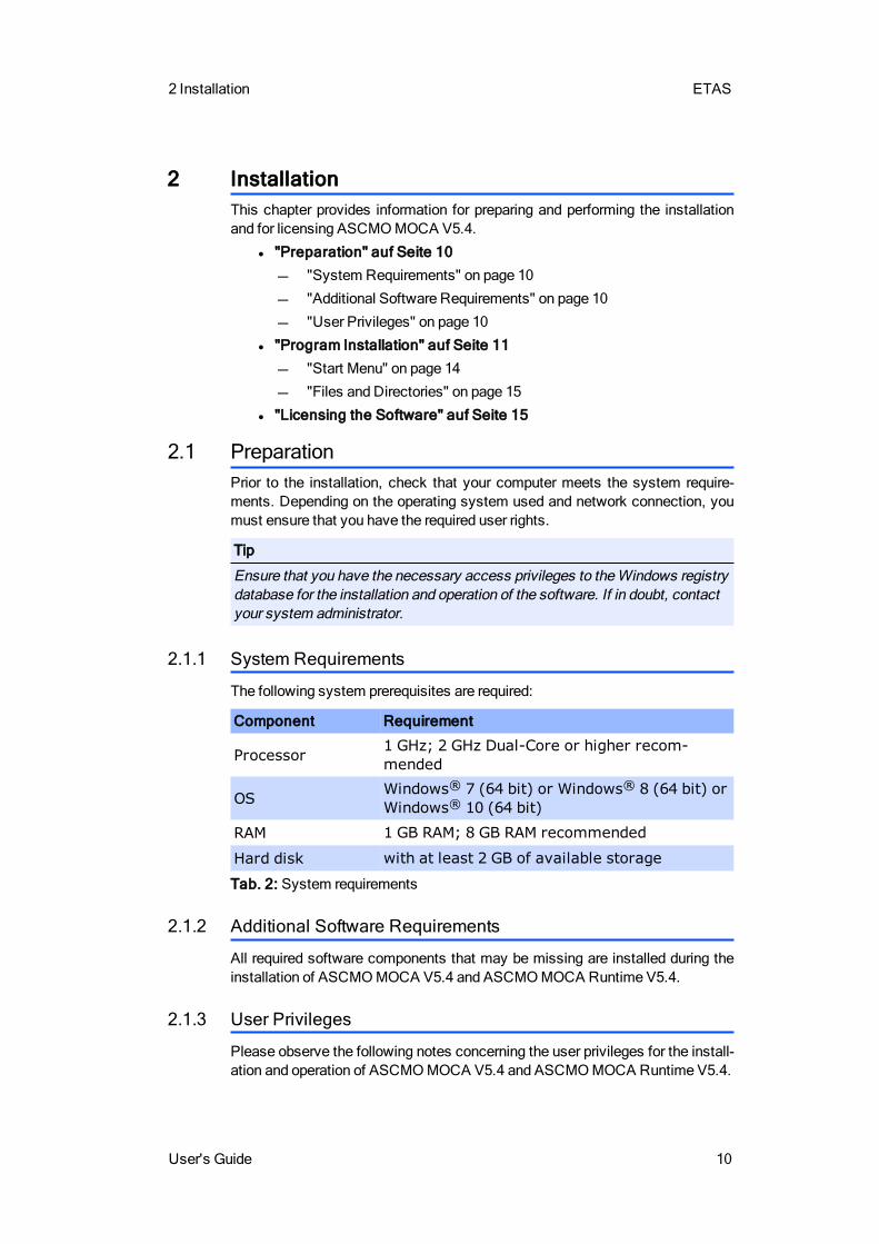
The following system prerequisites are required:
Component Requirement
Processor 1 GHz; 2 GHz Dual-Core or higher recom-mended
OS Windows® 7 (64 bit) or Windows® 8 (64 bit) orWindows® 10 (64 bit)
RAM 1 GB RAM; 8 GB RAM recommended
Hard disk with at least 2 GB of available storage
Tab. 2: System requirements
2.1.2 Additional Software Requirements
All required software components that may be missing are installed during theinstallation of ASCMOMOCA V5.4 and ASCMOMOCA Runtime V5.4.
2.1.3 User Privileges
Please observe the following notes concerning the user privileges for the install-ation and operation of ASCMOMOCA V5.4 and ASCMOMOCA Runtime V5.4.
ETAS 2 Installation
11 User's Guide
Required User Privileges for the InstallationTo install ASCMO MOCA V5.4 and ASCMO MOCA Runtime V5.4 on the PC,you require the user privileges of an administrator. If necessary, contact yoursystem administrator.
Required User Privileges for the OperationTo operate ASCMOMOCA V5.4 and ASCMOMOCA Runtime V5.4, privilegesof a standard user are sufficient.
2.2 Program Installation
Starting the installation
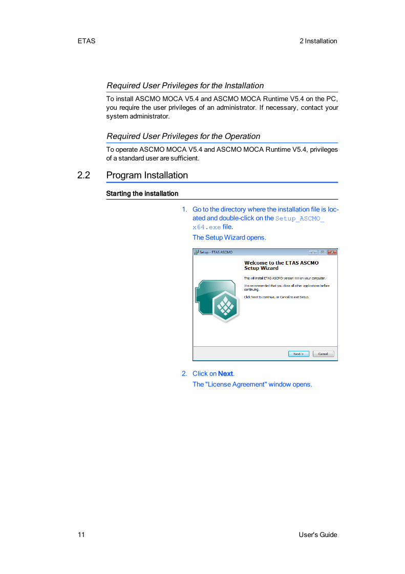
1. Go to the directory where the installation file is loc-ated and double-click on the Setup_ASCMO_x64.exe file.
The SetupWizard opens.
2. Click on Next.
The "License Agreement" window opens.
2 Installation ETAS
User's Guide 12
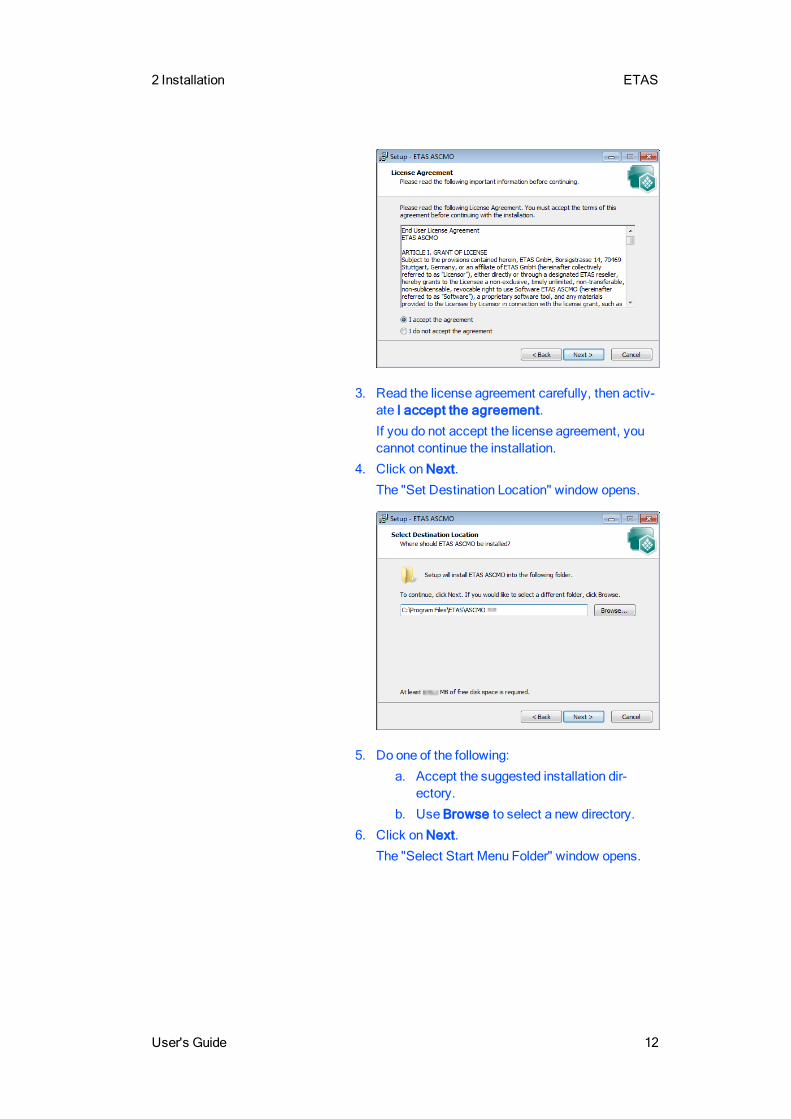
3. Read the license agreement carefully, then activ-ate I accept the agreement.
If you do not accept the license agreement, youcannot continue the installation.
4. Click on Next.
The "Set Destination Location" window opens.
5. Do one of the following:
a. Accept the suggested installation dir-ectory.
b. Use Browse to select a new directory.
6. Click on Next.
The "Select Start Menu Folder" window opens.
ETAS 2 Installation
13 User's Guide
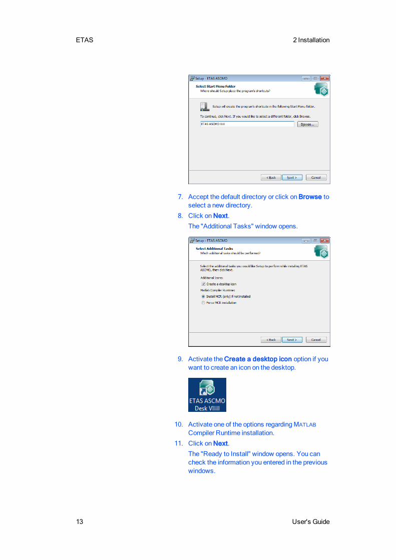
7. Accept the default directory or click on Browse toselect a new directory.
8. Click on Next.
The "Additional Tasks" window opens.
9. Activate the Create a desktop icon option if youwant to create an icon on the desktop.
10. Activate one of the options regardingMATLAB
Compiler Runtime installation.
11. Click on Next.
The "Ready to Install" window opens. You cancheck the information you entered in the previouswindows.
2 Installation ETAS
User's Guide 14
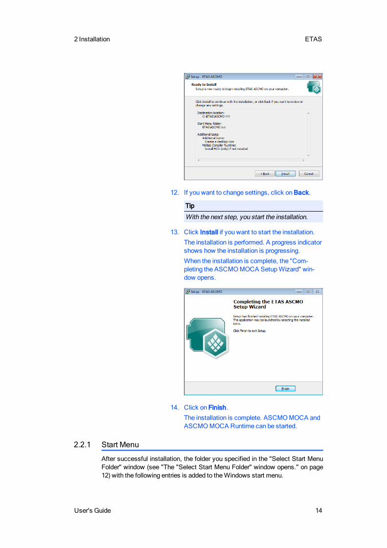
12. If you want to change settings, click on Back.
Tip
With the next step, you start the installation.
13. Click Install if you want to start the installation.
The installation is performed. A progress indicatorshows how the installation is progressing.
When the installation is complete, the "Com-pleting the ASCMOMOCA SetupWizard" win-dow opens.
14. Click on Finish.
The installation is complete. ASCMOMOCA andASCMOMOCA Runtime can be started.
2.2.1 Start Menu
After successful installation, the folder you specified in the "Select Start MenuFolder" window (see "The "Select Start Menu Folder" window opens." on page12) with the following entries is added to theWindows start menu.
ETAS 2 Installation
15 User's Guide
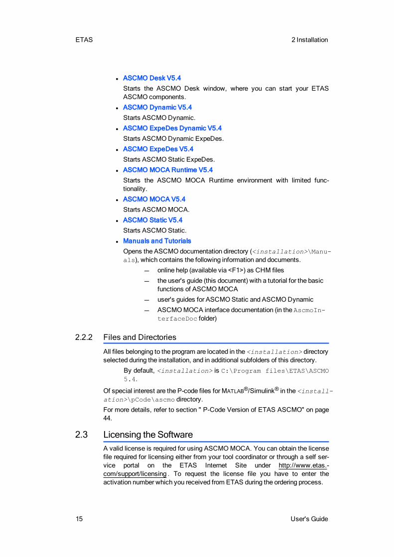
l ASCMO Desk V5.4
Starts the ASCMO Desk window, where you can start your ETASASCMO components.
l ASCMO Dynamic V5.4
Starts ASCMODynamic.
l ASCMO ExpeDes Dynamic V5.4
Starts ASCMODynamic ExpeDes.
l ASCMO ExpeDes V5.4
Starts ASCMOStatic ExpeDes.
l ASCMO MOCA Runtime V5.4
Starts the ASCMO MOCA Runtime environment with limited func-tionality.
l ASCMO MOCA V5.4
Starts ASCMOMOCA.
l ASCMO Static V5.4
Starts ASCMOStatic.
l Manuals and Tutorials
Opens the ASCMO documentation directory (<installation>\Manu-als), which contains the following information and documents.
online help (available via <F1>) as CHM files
the user's guide (this document) with a tutorial for the basicfunctions of ASCMOMOCA
user's guides for ASCMOStatic and ASCMODynamic
ASCMOMOCA interface documentation (in the AscmoIn-terfaceDoc folder)
2.2.2 Files and Directories
All files belonging to the program are located in the <installation> directoryselected during the installation, and in additional subfolders of this directory.
By default, <installation> is C:\Program files\ETAS\ASCMO5.4.
Of special interest are the P-code files for MATLAB®/Simulink® in the <install-ation>\pCode\ascmo directory.
For more details, refer to section " P-Code Version of ETAS ASCMO" on page44.
2.3 Licensing the SoftwareA valid license is required for using ASCMOMOCA. You can obtain the licensefile required for licensing either from your tool coordinator or through a self ser-vice portal on the ETAS Internet Site under http://www.etas.-com/support/licensing . To request the license file you have to enter theactivation number which you received from ETAS during the ordering process.
2 Installation ETAS
User's Guide 16
In the Windows Start menu, select Programs → ETAS → License Man-agement → ETAS License Manager.Follow the instructions given in the dialog. For further information about, forexample, the ETAS license models and borrowing a license, press <F1> in theETAS LicenseManager.
2.4 Uninstallation
Tip
You cannot uninstall only ASCMOMOCA. The procedure uninstalls all ETASASCMO components.
Use one of the following ways to start the ETAS ASCMO uninstall process:
l Programs and Features from theWindows control panel
Uninstalling ETAS ASCMO
1. Start the uninstall procedure.
A safety inquiry opens.
2. Click on Yes to continue.
ETAS ASCMO is uninstalled. A progress indic-ator shows how the uninstallation is progressing.
When the uninstallation is complete, a successwindow opens.
3. Click onOK to end the uninstallation.
ETAS 3Concepts of ETAS ASCMOMOCA
17 User's Guide
3 Concepts of ETAS ASCMO MOCAETAS ASCMO MOCA enables optimization of model parameters and min-imizes the deviation of model prediction and desired output values.
E.g. modern vehicle ECUs contain physically based models to replace or mon-itor real sensors. Such a physically based model is generic, but must be adap-ted to an actual engine. Parameters (maps/curves/scalars) are optimized usingreal measurements, e.g., from test bench or vehicle.
The model can be represented in ASCMO MOCA as a set of formulas enteredby the user. Alternatively, existingmodels, e.g. from Simulink®, can be used.
In this chapter, you can find a description of the basic concepts of ASCMOMOCA.
These are the following:
l "Fields of Application" on page 17
This section provides a general overview of the wide range of applicationfields in ASCMOMOCA.
l "Main Elements of the User Interface" on page 20
This section provides an brief overview of the user interface key ele-ments of ASCMOMOCA.
l "Data" on page 23
This section provides information on import, analysis and preprocessingof measured data.
l " " on page 31
This section provides information on importing and using external modelsin ASCMOMOCA.
l "Functions" on page 33
This section provides information on how to create amodel by specifyinga set of formulas that form a function.
l "Parameters " on page 35
This section contains general information about the optimization of para-meters within ASCMOMOCA.
l "Optimization" on page 39
This section contains a description of the different optimization methodsand the optimization criteria that can be used for the parameter optim-ization.
l " P-Code Version of ETAS ASCMO" on page 44
This section provides basic information on how to start ASCMO toolsfrom within MATLAB.
3.1 Fields of ApplicationThis section provides a general overview of the wide range of application fieldsof ASCMOMOCA.
3 Concepts of ETAS ASCMOMOCA ETAS
User's Guide 18
3.1.1 Fields of Application of ASCMOMOCA
Calibration of ECU Sensor Data
l Optimization of parameters
l Optimization of time-dependent (dynamic) functions
l Parameterization of ECU models (cylinder fill, torque, ...)
The use of ASCMO MOCA in the area of calibration offers a series of advant-ages:
l Significant increase in efficiency through reducedmeasuring and ana-lysis efforts
l Improved complexity handling
l Improved data quality
l Multiple use of models
Research, Function and System Development
l Quick calibration and evaluation of experimental engines
l Use of models of real engines for test and development of new functions(e.g., controller strategies)
l Analysis and optimization of unknown systems.
The advantages in the area of research and development lie primarily in aquicker andmore improved system understanding, coupled with a variety of pos-sibilities for impact analysis.
3.1.2 Fields of Application of ASCMOMOCA Runtime
The Runtime version of ASCMOMOCA is designed to fulfill the special require-ments of using the software with limited access to special functionalities.Reasons for doing this are to hide away special IP or to avoid that an userchanges something critical.
This version can be either installed and used in parallel to the main (Developer)version or as standalone.
Tip
The Runtime version does not allow to create or modify functions.
The following activities can be carried out with ASCMOMOCA Runtime:
l Import of stationary or transient data followed by name-mapping.
l Definition of conversion rules (Conversion Parameters / formulas).
l Import, export, creation, deletion and editing of parameters and systemconstants.
l Iterative optimization and calibration of parameters.
The installation of ASCMO MOCA Runtime is particularly recommended if theone who has created the project with the optimization task is not the same asthe one who executes the optimization.
This supports intellectual property protection and safety:

ETAS 3Concepts of ETAS ASCMOMOCA
19 User's Guide
l You do not have to share special know-how about the function or theoptimization logic with others.
l No critical parameters and settings are changed by the user who per-forms the optimization. Such changes could result in unexpected beha-vior.
3 Concepts of ETAS ASCMOMOCA ETAS
User's Guide 20
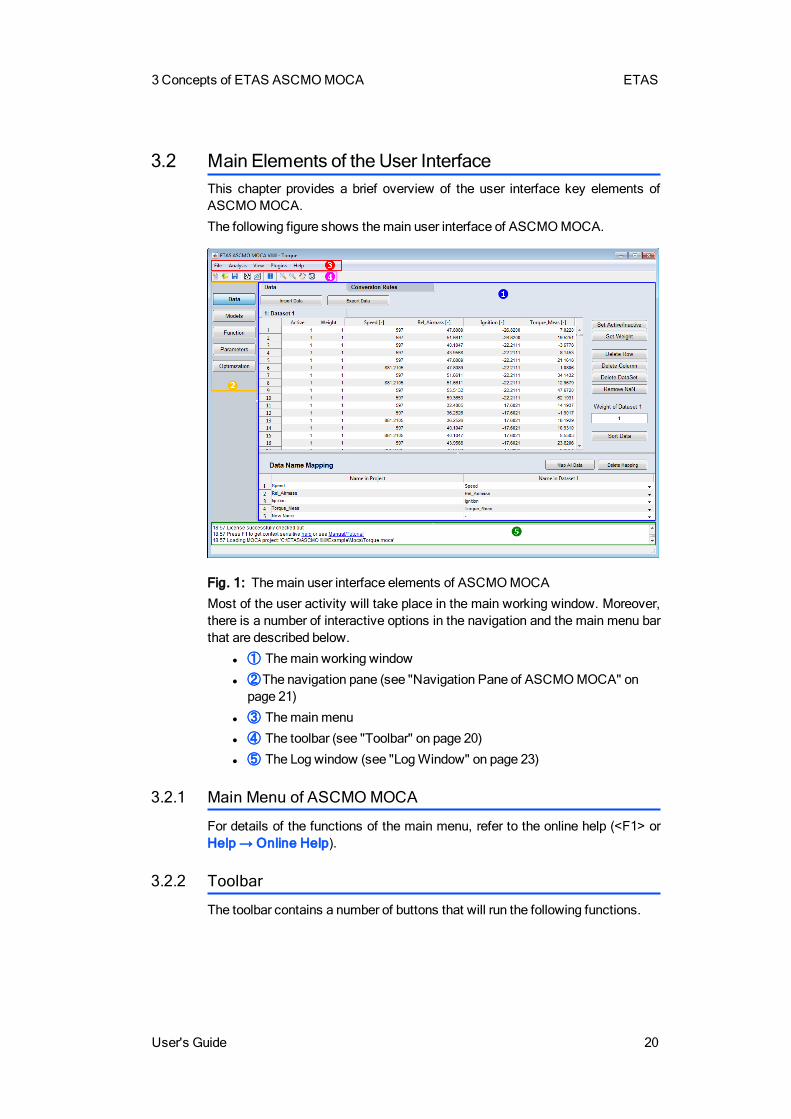
3.2 Main Elements of the User InterfaceThis chapter provides a brief overview of the user interface key elements ofASCMOMOCA.
The following figure shows themain user interface of ASCMOMOCA.
Fig. 1: Themain user interface elements of ASCMOMOCA
Most of the user activity will take place in the main working window. Moreover,there is a number of interactive options in the navigation and the main menu barthat are described below.
l ➀ Themain working window
l ➁The navigation pane (see "Navigation Pane of ASCMOMOCA" onpage 21)
l ➂ Themainmenu
l ➃ The toolbar (see "Toolbar" on page 20)
l ➄ The Log window (see "LogWindow" on page 23)
3.2.1 Main Menu of ASCMOMOCA
For details of the functions of the main menu, refer to the online help (<F1> orHelp → Online Help).
3.2.2 Toolbar
The toolbar contains a number of buttons that will run the following functions.
ETAS 3Concepts of ETAS ASCMOMOCA
21 User's Guide
New Project Opens a new instance of ASCMOMOCA.
Open Project Opens a data selection dialog where youcan open available projects (*.moca).
Save Saves the current project.
Scatter Plot for TrainingData
Opens the "Data and Nodes - TrainingData" window.
See also "Graphical Analysis of Data andFunction Nodes" on page 25.
Scope View for TrainingData
Opens the "Scope View - Training Data"window.
Pause evaluation ofexternal models, e.g.FMI
Pauses the execution of an importedmodel.
Zoom In By clicking in the plot, the visualizationbecomes larger.
ZoomOut By clicking in the plot, the visualizationbecomes smaller.
Pan This button allows you tomove the plotwithin the window.
Rotate 3D This button allows you to rotate a plot in alldimensions.
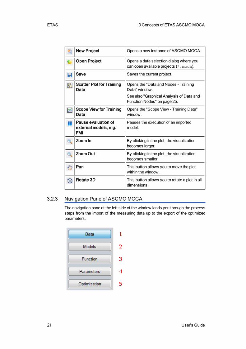
3.2.3 Navigation Pane of ASCMOMOCA
The navigation pane at the left side of the window leads you through the processsteps from the import of the measuring data up to the export of the optimizedparameters.

3 Concepts of ETAS ASCMOMOCA ETAS
User's Guide 22
1. Data
Opens the Data Step in the main working window. Here, you can importa measurement file, edit the measurement data and export the data to ameasurement file. In addition, the data channel from the measurementfile can be mapped to the respective function variable (Data Name Map-ping).
Further information can be found in "Data" on page 23, in the tutorial (see"Step 1: Data Import" on page 49), and in the online help.
2. Models
Opens the Models Step in the main working window. You can add mod-els and link the parameters, inputs and outputs with the available para-meters in ASCMOMOCA.
Tip
To use a Simulink model in ASCMOMOCA, Simulink installation with avalid license is required.
Further information can be found in section " " on page 31, in the tutorial(see "Step 3: Models" on page 71), and in the online help.
3. Function
Opens the Function Step in the main working window. The function willbe constructed from the stepwise creation of the nodes. The main pointhere is the linkage of the parameters and the data.
Further information can be found in "Functions" on page 33, in the tutorial(see "Step 4: Build Up the Function" on page 82), and in the online help.
4. Parameters
Opens the Parameters Step in the main working window. Here, you canmanage and change maps, curves, scalars, cube-3D, cube-4D cube,compressedmodel andmatrix for the usage in the Function Step.
Further information can be found in "Parameters " on page 35, in thetutorial (see "Step 5: Parameters" on page 91), and in the online help.
5. Optimization
Opens the Optimization Step in the main working window. The para-meter optimization takes place in the main working area of the optim-ization pane. Within this pane, the following major tasks can beperformed:
l Definition of the parameter-related optimization criterion (e.g.,smoothness, gradient constraints).
l Determination of parameters as reference for the comparison withfollowing optimization results.
l Export of optimized parameters.
After performing these tasks, you can start the optimization.
Further information can be found in "Optimization" on page 39, in thetutorial (see "Step 6: Optimization" on page 92), and in the online help.
ETAS 3Concepts of ETAS ASCMOMOCA
23 User's Guide
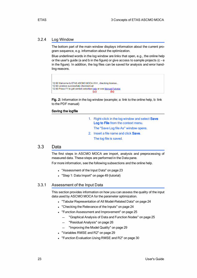
3.2.4 Log Window
The bottom part of the main window displays information about the current pro-gram sequence, e.g. information about the optimization.
Blue underlined words in the log window are links that open, e.g., the online helpor the user's guide (a and b in the figure) or give access to sample projects (c - ein the figure). In addition, the log files can be saved for analysis and error hand-ling reasons.
Fig. 2: Information in the log window (example; a: link to the online help, b: linkto the PDFmanual)
Saving the logfile
1. Right-click in the log window and select SaveLog to File from the context menu.
The "Save Log file As" window opens.
2. Insert a file name and click Save.
The log file is saved.
3.3 DataThe first steps in ASCMO MOCA are import, analysis and preprocessing ofmeasured data. These steps are performed in the Data pane.
For more information, see the following subsections and the online help.
l "Assessment of the Input Data" on page 23
l "Step 1: Data Import" on page 49 (tutorial)
3.3.1 Assessment of the Input Data
This section provides information on how you can assess the quality of the inputdata used by ASCMOMOCA for the parameter optimization.
l "Tabular Representation of All Model-Related Data" on page 24
l "Checking the Relevance of the Inputs" on page 24
l "Function Assessment and Improvement" on page 25
"Graphical Analysis of Data and Function Nodes" on page 25
"Residual Analysis" on page 26
"Improving theModel Quality" on page 29
l "Variables RMSE and R2" on page 29
l "Function Evaluation Using RMSE and R2" on page 30
3 Concepts of ETAS ASCMOMOCA ETAS
User's Guide 24
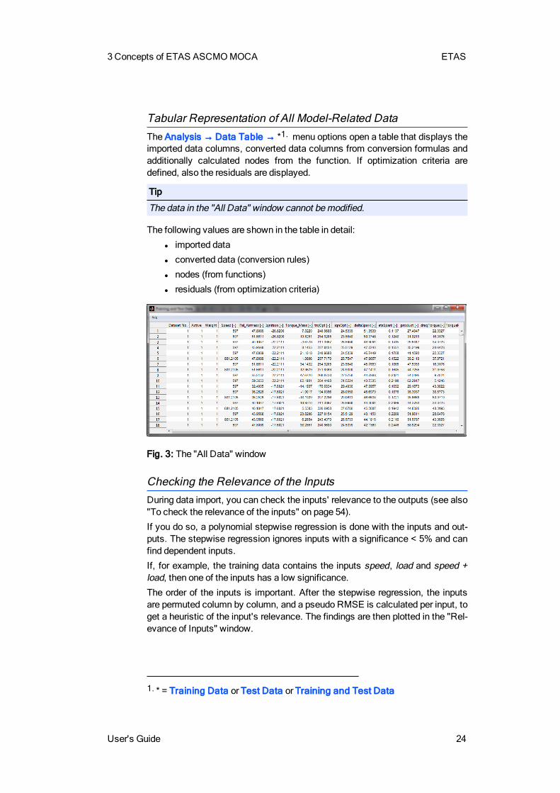
Tabular Representation of All Model-Related DataThe Analysis → Data Table → *1. menu options open a table that displays theimported data columns, converted data columns from conversion formulas andadditionally calculated nodes from the function. If optimization criteria aredefined, also the residuals are displayed.
Tip
The data in the "All Data" window cannot bemodified.
The following values are shown in the table in detail:
l imported data
l converted data (conversion rules)
l nodes (from functions)
l residuals (from optimization criteria)
Fig. 3: The "All Data" window
Checking the Relevance of the InputsDuring data import, you can check the inputs' relevance to the outputs (see also"To check the relevance of the inputs" on page 54).
If you do so, a polynomial stepwise regression is done with the inputs and out-puts. The stepwise regression ignores inputs with a significance < 5% and canfind dependent inputs.
If, for example, the training data contains the inputs speed, load and speed +load, then one of the inputs has a low significance.
The order of the inputs is important. After the stepwise regression, the inputsare permuted column by column, and a pseudo RMSE is calculated per input, toget a heuristic of the input's relevance. The findings are then plotted in the "Rel-evance of Inputs" window.
1. * = Training Data or Test Data or Training and Test Data
ETAS 3Concepts of ETAS ASCMOMOCA
25 User's Guide
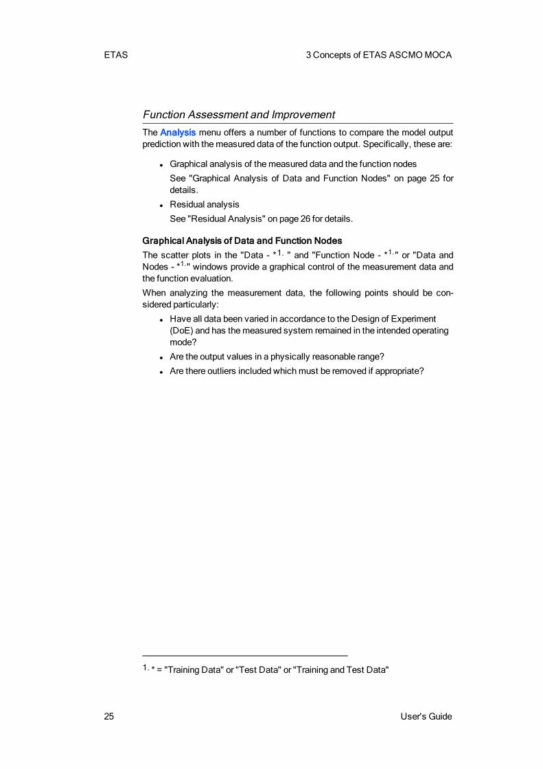
Function Assessment and ImprovementThe Analysis menu offers a number of functions to compare the model outputprediction with themeasured data of the function output. Specifically, these are:
l Graphical analysis of themeasured data and the function nodes
See "Graphical Analysis of Data and Function Nodes" on page 25 fordetails.
l Residual analysis
See "Residual Analysis" on page 26 for details.
Graphical Analysis of Data and Function Nodes
The scatter plots in the "Data - *1. " and "Function Node - *1." or "Data andNodes - *1." windows provide a graphical control of the measurement data andthe function evaluation.
When analyzing the measurement data, the following points should be con-sidered particularly:
l Have all data been varied in accordance to the Design of Experiment(DoE) and has themeasured system remained in the intended operatingmode?
l Are the output values in a physically reasonable range?
l Are there outliers included whichmust be removed if appropriate?
1. * = "Training Data" or "Test Data" or "Training and Test Data"
3 Concepts of ETAS ASCMOMOCA ETAS
User's Guide 26
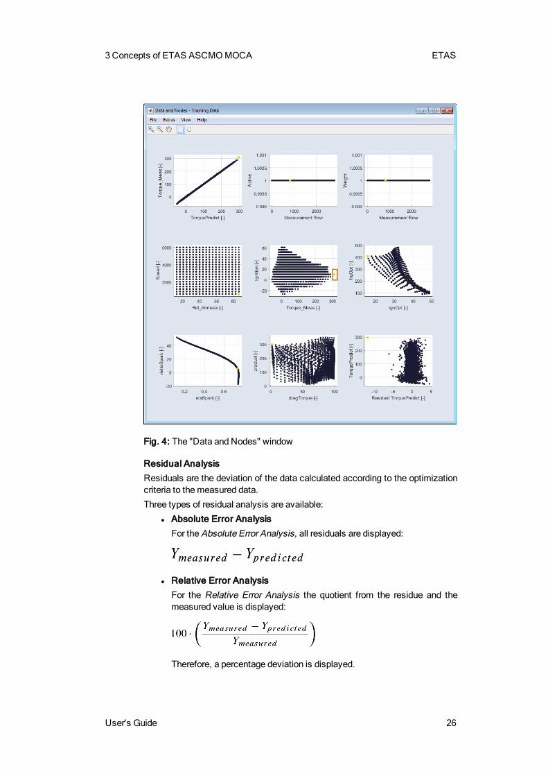
Fig. 4: The "Data and Nodes" window
Residual Analysis
Residuals are the deviation of the data calculated according to the optimizationcriteria to themeasured data.
Three types of residual analysis are available:
l Absolute Error Analysis
For the Absolute Error Analysis, all residuals are displayed:
l Relative Error Analysis
For the Relative Error Analysis the quotient from the residue and themeasured value is displayed:
Therefore, a percentage deviation is displayed.
ETAS 3Concepts of ETAS ASCMOMOCA
27 User's Guide
l Studentized Error Analysis
When performing a Studentized error analysis , the quotient from theresidual and the RMSE (see "RMSE (Root Mean Squared Error)" onpage 29) is displayed:
Thus, the error based on the RMSE is shown.
Residual analysis is performed via the Analysis → Residual Analysis → *menu options. Thesemenu options open four plot windows:
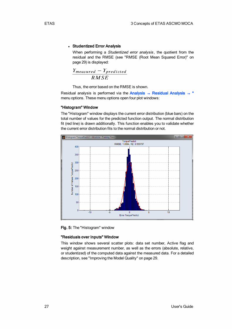
"Histogram" Window
The "Histogram" window displays the current error distribution (blue bars) on thetotal number of values for the predicted function output. The normal distributionfit (red line) is drawn additionally. This function enables you to validate whetherthe current error distribution fits to the normal distribution or not.
Fig. 5: The "Histogram" window
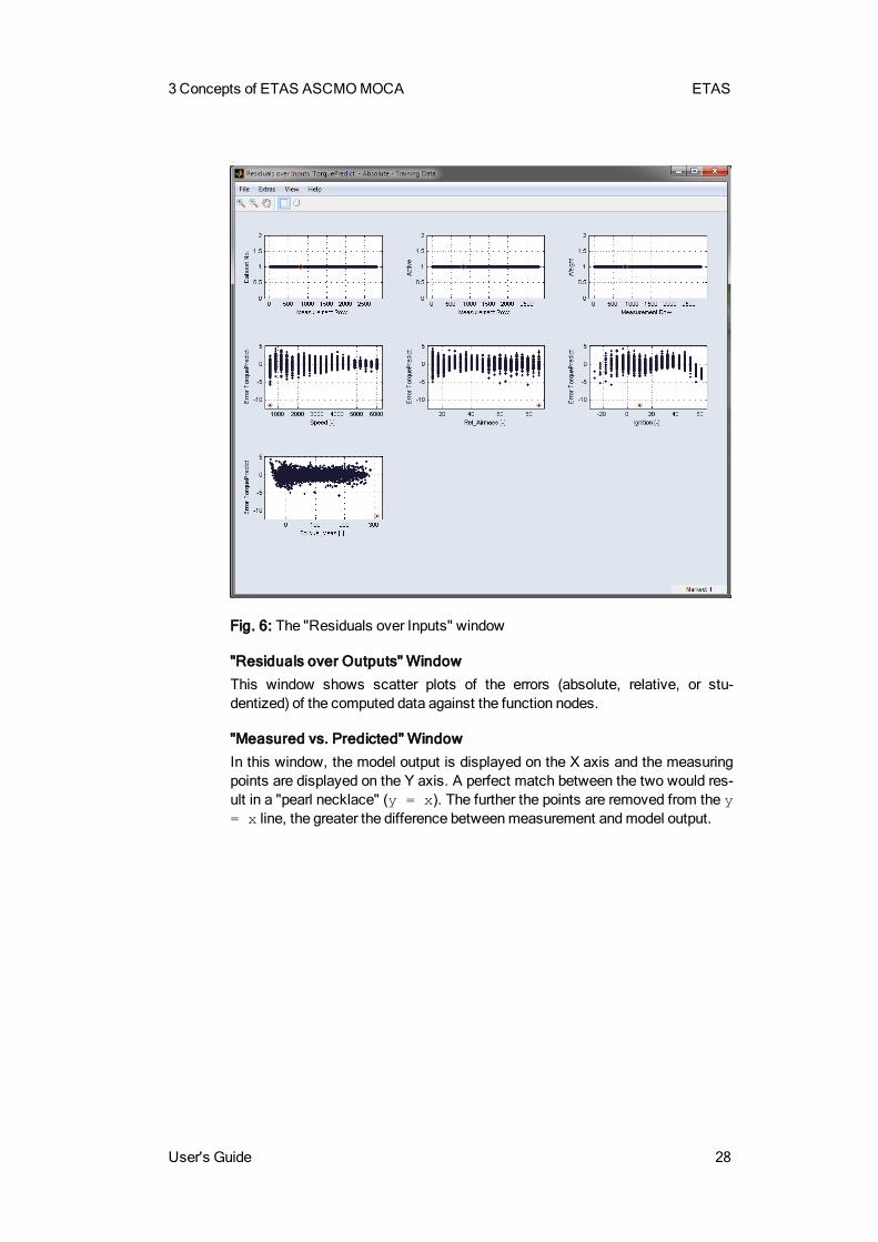
"Residuals over Inputs" Window
This window shows several scatter plots: data set number, Active flag andweight against measurement number, as well as the errors (absolute, relative,or studentized) of the computed data against the measured data. For a detaileddescription, see "Improving theModel Quality" on page 29.
3 Concepts of ETAS ASCMOMOCA ETAS
User's Guide 28
Fig. 6: The "Residuals over Inputs" window
"Residuals over Outputs" Window
This window shows scatter plots of the errors (absolute, relative, or stu-dentized) of the computed data against the function nodes.
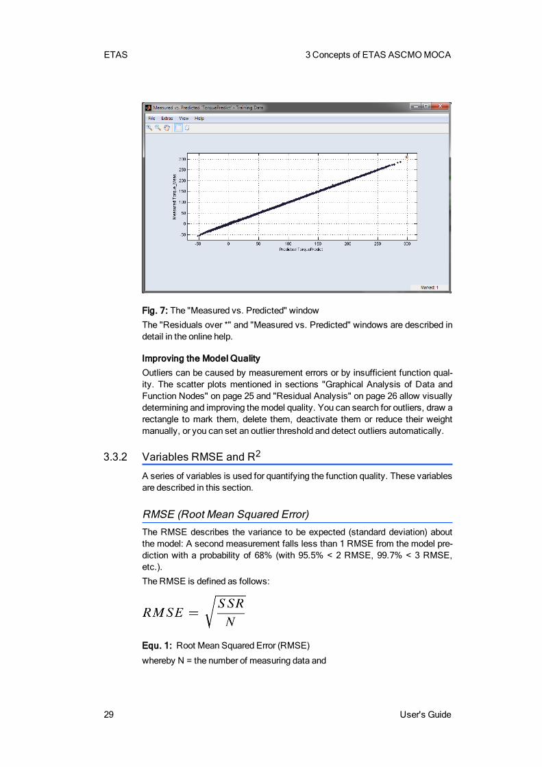
"Measured vs. Predicted" Window
In this window, the model output is displayed on the X axis and the measuringpoints are displayed on the Y axis. A perfect match between the two would res-ult in a "pearl necklace" (y = x). The further the points are removed from the y= x line, the greater the difference betweenmeasurement andmodel output.
ETAS 3Concepts of ETAS ASCMOMOCA
29 User's Guide
Fig. 7: The "Measured vs. Predicted" window
The "Residuals over *" and "Measured vs. Predicted" windows are described indetail in the online help.
Improving the Model Quality
Outliers can be caused by measurement errors or by insufficient function qual-ity. The scatter plots mentioned in sections "Graphical Analysis of Data andFunction Nodes" on page 25 and "Residual Analysis" on page 26 allow visuallydetermining and improving themodel quality. You can search for outliers, draw arectangle to mark them, delete them, deactivate them or reduce their weightmanually, or you can set an outlier threshold and detect outliers automatically.
3.3.2 Variables RMSE and R2
A series of variables is used for quantifying the function quality. These variablesare described in this section.
RMSE (Root Mean Squared Error)The RMSE describes the variance to be expected (standard deviation) aboutthe model: A second measurement falls less than 1 RMSE from the model pre-diction with a probability of 68% (with 95.5% < 2 RMSE, 99.7% < 3 RMSE,etc.).
The RMSE is defined as follows:
Equ. 1: Root Mean Squared Error (RMSE)
whereby N = the number of measuring data and

3 Concepts of ETAS ASCMOMOCA ETAS
User's Guide 30
Equ. 2: Sum of Squared Residuals (SSR)
Therefore, SSR is the sum of squared residuals (SSR = Sum of Squared Resid-uals).
Coefficient of Determination R2The coefficient of determination R2 is derived from the comparison of the vari-ance that remains after the model training (SSR) with the variance concerningthemean value of all measuring data (SST)
Equ. 3: Coefficient of determination R2
whereby
Equ. 4: Total Sum of Squares (SST)
R2 is a relative measure for evaluating the function output error – it indicateswhich portion of the total variance of the measuring data is described by thefunction.
3.3.3 Function Evaluation Using RMSE and R2
Evaluation of R2The most important variable is the coefficient of determination R2 ("Coefficientof Determination R2" on page 30) . This measure results in the following eval-uations:
l The coefficient of determination, R2, can bemaximal 1. In this case, thefunction prediction fits exactly to eachmeasured value.
l If the function would simply predict the mean of the measured output forany input data, an R2 of 0 would be the result. A negative R2 would meanthat the prediction is worse than that simple prediction.
l An R2 of 1 means a perfect fit, every prediction of the function is thesame as the measured data. Typically, the measured data has addednoise. In this case, an R2 of 1 means overfitting. You should be inter-ested in a high R2with consideration of the noise.
l Keep in mind that different signals can be measured with different qual-ity. There might be signals where an R2 of 0.6 might already be a good
ETAS 3Concepts of ETAS ASCMOMOCA
31 User's Guide
value. In contrast, a model for a different signal can be seen as good onlyif the R2 is above 0.99.
Evaluation of RMSEThe absolute error RMSE (see section "RMSE (Root Mean Squared Error)" onpage 29) must be evaluated individually:
l At best, the RMSE can be as good as the experimental repeatability.
l Despite a good R2, the RMSE can be too low, e. g. in case of a verylarge variation range of themodeled variable.
l Despite a small R2, the RMSE can be good enough, e. g. if themodeledvariable features only aminor variance over the input parameters of thefunction.
3.4
3.5 ModelsIn ASCMO MOCA, you can work with models provided as a set of formulas, oryou can import models created with ASCET, FMU, Simulink, ASCMO Static orASCMO Dynamic. These models can then be used as function nodes in theASCMOMOCA project.
Importing and connecting external models is done in theModels pane.
l ASCETmodels
If you want to use an ASCET model in ASCMOMOCA, you have to cre-ate a *.dll file with ASCET and ASCET-PSL first. This *.dll file isthen added to the ASCMOMOCA project; see the online help for details.
ASCET models are used as black boxes by MOCA. You cannot changethe models, and no link to the ASCET model or to ASCET is created dur-ing import.
l FMU models
If you want to use a FMU model in ASCMO MOCA, you have to createan FMI 2.x *.fmu file first. This *.fmu file is then added to the ASCMOMOCA project; see the online help for details.
Tip
Only FMU models that use FMI 2.x are supported by ASCMOMOCA.FMU models that use FMI 1 cannot be used.
Only the FMU file name is added to the MOCA project. You cannot openthe model itself. During optimization, the FMU model is used as a blackbox: MOCA passes the inputs to the model, and receives the outputsfrom the model. The way the model computes the output values remainsunknown toMOCA.
l Simulink models
3 Concepts of ETAS ASCMOMOCA ETAS
User's Guide 32
Using Simulink models in ASCMO MOCA is described in detail in thetutorial, see "Step 3: Models" on page 71.
l ASCMOStatic and ASCMODynamic models
These models are used as black boxes. You cannot change the models,and no link to the ASCMO Static/ASCMO Dynamic models or to theASCMO tools is created during import.
During import, you can select one, several or all outputs for import. Eachoutput is added as a separate model. See also section " ImportingASCMOStatic/ASCMODynamic Models" in the online help.
For more information, see the online help.
ETAS 3Concepts of ETAS ASCMOMOCA
33 User's Guide
3.6 FunctionsIn ASCMO MOCA, you can work with models provided as a set of formulas, oryou can import models created with Simulink, ASCET, ASCMO Static orASCMODynamic and connect them to the ASCMOMOCA project.
Specifying a function formed by a set of formulas is done in the Function pane.
Data channels, parameters, other function nodes and imported models can beused to define the expression of a function node. Several operators are avail-able; see "Mathematical Operators for Function Nodes" on page 33.
You can export and import functions to and from text files that follow the formulasyntax. A sample export file is given here.
trqOpt[-] = %MapOptTorque%(%Speed%,%Rel_Airmass%)
ignOpt[-] = %MapOptIgnition%(%Speed%,%Rel_Airmass%)
deltaSpark[-] = %ignOpt% - %Ignition%
etaSpark[-] = %CurveEtaDeltaSpark%(%deltaSpark%)
product [-] = %SubFunction% (%deltaSpark%, %trqOpt%,%CurveEtaDeltaSpark%)
dragTorque[-] = %MapDragTorque%(%Speed%,%Rel_Airmass%)
TorquePredict[-] = %product% - %dragTorque%
function SubFunction(InDeltaSpark : Data, IntrqOpt :Data, myCurve : Curve)
curveOut[-] = %myCurve%(%InDeltaSpark%)
functionOut[-] = %curveOut% .* %IntrqOpt%
Formore information, see the following subsections and the online help.
l "Mathematical Operators for Function Nodes" on page 33
l "Step 4: Build Up the Function" on page 82 (tutorial)
3.6.1 Mathematical Operators for Function Nodes
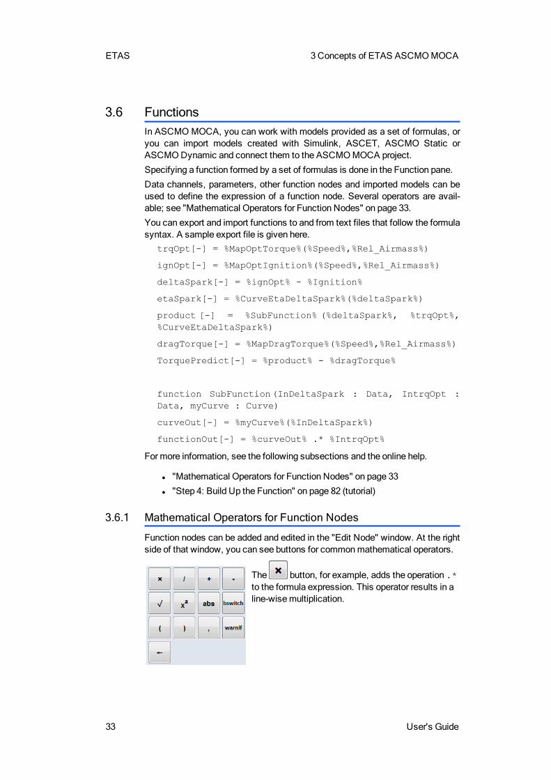
Function nodes can be added and edited in the "Edit Node" window. At the rightside of that window, you can see buttons for commonmathematical operators.
The button, for example, adds the operation .*to the formula expression. This operator results in aline-wisemultiplication.
3 Concepts of ETAS ASCMOMOCA ETAS
User's Guide 34
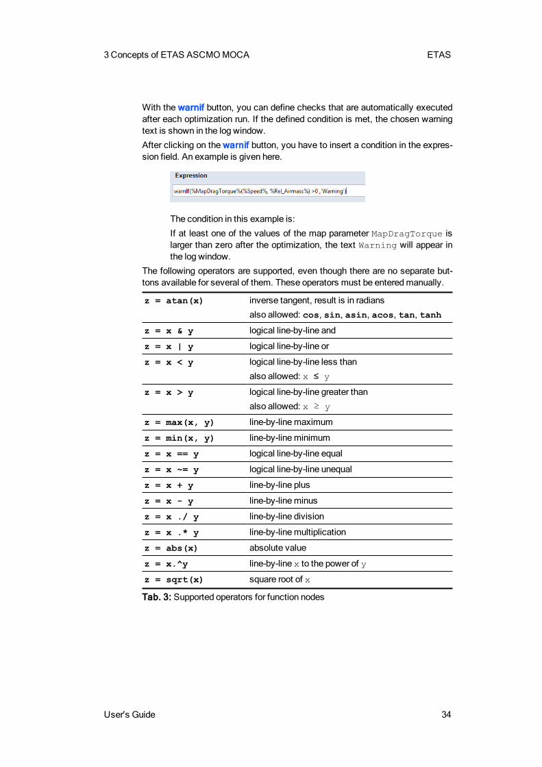
With the warnif button, you can define checks that are automatically executedafter each optimization run. If the defined condition is met, the chosen warningtext is shown in the log window.
After clicking on the warnif button, you have to insert a condition in the expres-sion field. An example is given here.
The condition in this example is:
If at least one of the values of the map parameter MapDragTorque islarger than zero after the optimization, the text Warning will appear inthe log window.
The following operators are supported, even though there are no separate but-tons available for several of them. These operators must be enteredmanually.
z = atan(x) inverse tangent, result is in radians
also allowed: cos, sin, asin, acos, tan, tanh
z = x & y logical line-by-line and
z = x | y logical line-by-line or
z = x < y logical line-by-line less than
also allowed: x ≤ y
z = x > y logical line-by-line greater than
also allowed: x ≥ y
z = max(x, y) line-by-linemaximum
z = min(x, y) line-by-lineminimum
z = x == y logical line-by-line equal
z = x ~= y logical line-by-line unequal
z = x + y line-by-line plus
z = x - y line-by-lineminus
z = x ./ y line-by-line division
z = x .* y line-by-linemultiplication
z = abs(x) absolute value
z = x.^y line-by-line x to the power of y
z = sqrt(x) square root of x
Tab. 3: Supported operators for function nodes
ETAS 3Concepts of ETAS ASCMOMOCA
35 User's Guide
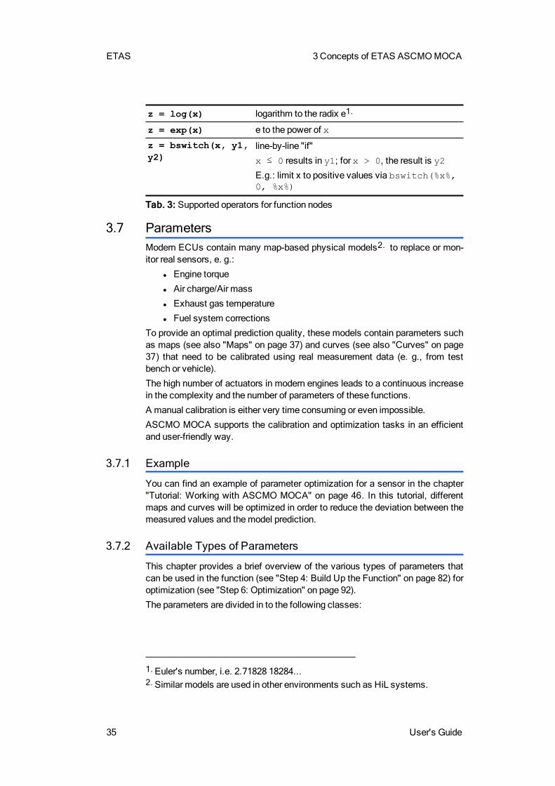
z = log(x) logarithm to the radix e1.
z = exp(x) e to the power of x
z = bswitch(x, y1,y2)
line-by-line "if"
x ≤ 0 results in y1; for x > 0, the result is y2
E.g.: limit x to positive values via bswitch(%x%,0, %x%)
Tab. 3: Supported operators for function nodes
3.7 ParametersModern ECUs contain many map-based physical models2. to replace or mon-itor real sensors, e. g.:
l Engine torque
l Air charge/Air mass
l Exhaust gas temperature
l Fuel system corrections
To provide an optimal prediction quality, these models contain parameters suchas maps (see also "Maps" on page 37) and curves (see also "Curves" on page37) that need to be calibrated using real measurement data (e. g., from testbench or vehicle).
The high number of actuators in modern engines leads to a continuous increasein the complexity and the number of parameters of these functions.
A manual calibration is either very time consuming or even impossible.
ASCMO MOCA supports the calibration and optimization tasks in an efficientand user-friendly way.
3.7.1 Example
You can find an example of parameter optimization for a sensor in the chapter"Tutorial: Working with ASCMO MOCA" on page 46. In this tutorial, differentmaps and curves will be optimized in order to reduce the deviation between themeasured values and themodel prediction.
3.7.2 Available Types of Parameters
This chapter provides a brief overview of the various types of parameters thatcan be used in the function (see "Step 4: Build Up the Function" on page 82) foroptimization (see "Step 6: Optimization" on page 92).
The parameters are divided in to the following classes:
1. Euler's number, i.e. 2.71828 18284...2. Similar models are used in other environments such as HiL systems.
3 Concepts of ETAS ASCMOMOCA ETAS
User's Guide 36
l "Maps" on page 37
l "Curves" on page 37
l "Scalar" on page 38
l "3D- and 4D-Cubes" on page 38
l "CompressedModel" on page 38
l "Matrix " on page 39
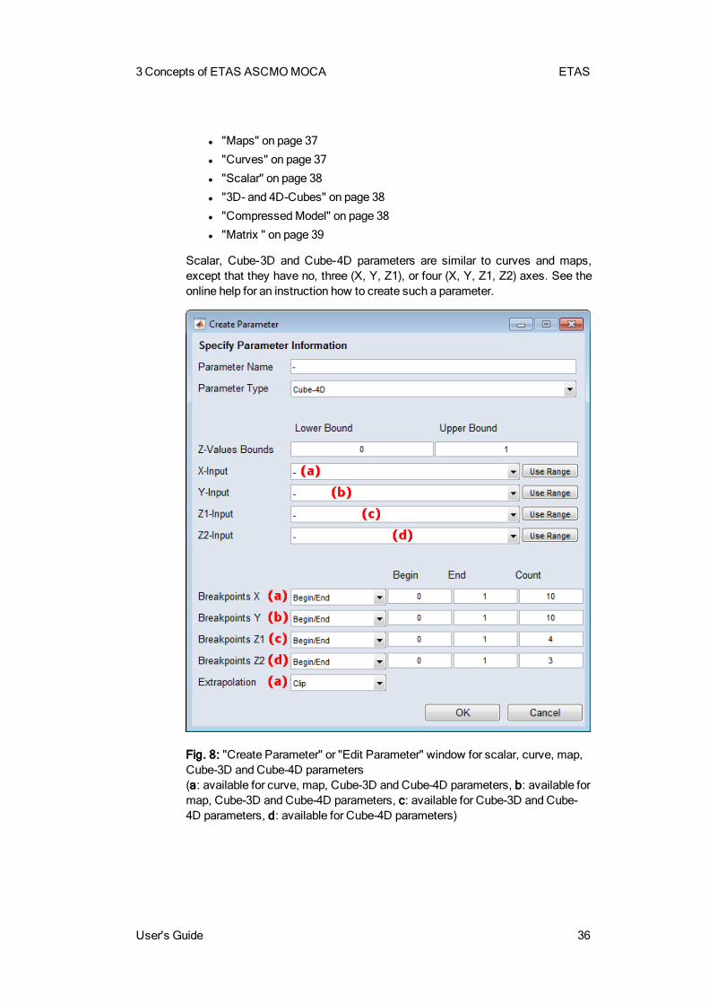
Scalar, Cube-3D and Cube-4D parameters are similar to curves and maps,except that they have no, three (X, Y, Z1), or four (X, Y, Z1, Z2) axes. See theonline help for an instruction how to create such a parameter.
Fig. 8: "Create Parameter" or "Edit Parameter" window for scalar, curve, map,Cube-3D and Cube-4D parameters(a: available for curve, map, Cube-3D and Cube-4D parameters, b: available formap, Cube-3D and Cube-4D parameters, c: available for Cube-3D and Cube-4D parameters, d: available for Cube-4D parameters)
ETAS 3Concepts of ETAS ASCMOMOCA
37 User's Guide
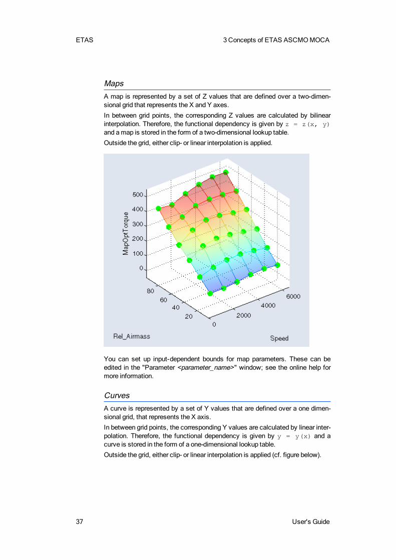
MapsA map is represented by a set of Z values that are defined over a two-dimen-sional grid that represents the X and Y axes.
In between grid points, the corresponding Z values are calculated by bilinearinterpolation. Therefore, the functional dependency is given by z = z(x, y)and amap is stored in the form of a two-dimensional lookup table.
Outside the grid, either clip- or linear interpolation is applied.
You can set up input-dependent bounds for map parameters. These can beedited in the "Parameter <parameter_name>" window; see the online help formore information.
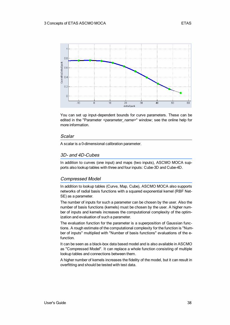
CurvesA curve is represented by a set of Y values that are defined over a one dimen-sional grid, that represents the X axis.
In between grid points, the corresponding Y values are calculated by linear inter-polation. Therefore, the functional dependency is given by y = y(x) and acurve is stored in the form of a one-dimensional lookup table.
Outside the grid, either clip- or linear interpolation is applied (cf. figure below).
3 Concepts of ETAS ASCMOMOCA ETAS
User's Guide 38
You can set up input-dependent bounds for curve parameters. These can beedited in the "Parameter <parameter_name>" window; see the online help formore information.
ScalarA scalar is a 0-dimensional calibration parameter.
3D- and 4D-CubesIn addition to curves (one input) and maps (two inputs), ASCMO MOCA sup-ports also lookup tables with three and four inputs: Cube-3D and Cube-4D.
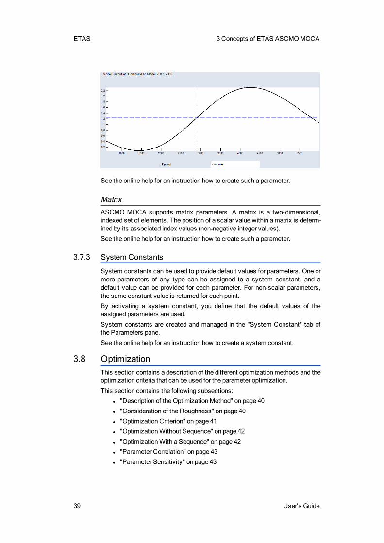
Compressed ModelIn addition to lookup tables (Curve, Map, Cube), ASCMO MOCA also supportsnetworks of radial basis functions with a squared exponential kernel (RBF Net-SE) as a parameter.
The number of inputs for such a parameter can be chosen by the user. Also thenumber of basis functions (kernels) must be chosen by the user. A higher num-ber of inputs and kernels increases the computational complexity of the optim-ization and evaluation of such a parameter.
The evaluation function for the parameter is a superposition of Gaussian func-tions. A rough estimate of the computational complexity for the function is "Num-ber of inputs" multiplied with "Number of basis functions" evaluations of the e-function.
It can be seen as a black-box data basedmodel and is also available in ASCMOas "Compressed Model". It can replace a whole function consisting of multiplelookup tables and connections between them.
A higher number of kernels increases the fidelity of themodel, but it can result inoverfitting and should be tested with test data.
ETAS 3Concepts of ETAS ASCMOMOCA
39 User's Guide
See the online help for an instruction how to create such a parameter.
MatrixASCMO MOCA supports matrix parameters. A matrix is a two-dimensional,indexed set of elements. The position of a scalar value within amatrix is determ-ined by its associated index values (non-negative integer values).
See the online help for an instruction how to create such a parameter.
3.7.3 System Constants
System constants can be used to provide default values for parameters. One ormore parameters of any type can be assigned to a system constant, and adefault value can be provided for each parameter. For non-scalar parameters,the same constant value is returned for each point.
By activating a system constant, you define that the default values of theassigned parameters are used.
System constants are created and managed in the "System Constant" tab ofthe Parameters pane.
See the online help for an instruction how to create a system constant.
3.8 OptimizationThis section contains a description of the different optimizationmethods and theoptimization criteria that can be used for the parameter optimization.
This section contains the following subsections:
l "Description of the OptimizationMethod" on page 40
l "Consideration of the Roughness" on page 40
l "Optimization Criterion" on page 41
l "OptimizationWithout Sequence" on page 42
l "OptimizationWith a Sequence" on page 42
l "Parameter Correlation" on page 43
l "Parameter Sensitivity" on page 43
3 Concepts of ETAS ASCMOMOCA ETAS
User's Guide 40
3.8.1 Description of the Optimization Method
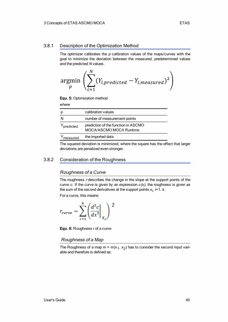
The optimizer calibrates the p calibration values of the maps/curves with thegoal to minimize the deviation between the measured, predetermined valuesand the predicted N values.
Equ. 5: Optimizationmethod
where
p calibration values
N number of measurement points
Ypredicted prediction of the function in ASCMOMOCA/ASCMOMOCA Runtime
Ymeasured the imported data
The squared deviation is minimized, where the square has the effect that largerdeviations are penalized even stronger.
3.8.2 Consideration of the Roughness
Roughness of a CurveThe roughness r describes the change in the slope at the support points of thecurve c. If the curve is given by an expression c(x), the roughness is given asthe sum of the second derivatives at the support points xi, i=1..k.
For a curve, this means:
Equ. 6: Roughness r of a curve
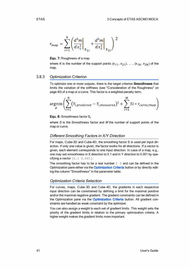
Roughness of a MapThe Roughness of a map m = m(x1, x2) has to consider the second input vari-able and therefore is defined as:
ETAS 3Concepts of ETAS ASCMOMOCA
41 User's Guide
Equ. 7: Roughness of amap
where K is the number of the support points (x11, x21), ... , (x1K, x2K) of themap.
3.8.3 Optimization Criterion
To optimize one or more outputs, there is the target criterion Smoothness thatlimits the variation of the stiffness (see "Consideration of the Roughness" onpage 40) of amap or a curve. This factor is a weighted penalty term,
Equ. 8: Smoothness factor Siwhere S is the Smoothness factor and M the number of support points of themap or curve.
Different Smoothing Factors in X/Y DirectionFor maps, Cube-3D and Cube-4D, the smoothing factor S is used per input dir-ection. If only one value is given, the factor works for all directions. If a vector isgiven, each element corresponds to one input direction. In case of a map, e.g.,one may set smoothness in X direction to 0.1 and in Y direction to 0.001 by spe-cifying a vector [0.1 0.001].
The smoothing factor has to be a real number ≥ 0 and can be defined in theOptimization pane either via the Optimization Criteria button or by directly edit-ing the column "Smoothness" in the parameter table.
Optimization Criteria SelectionFor curves, maps, Cube-3D and Cube-4D, the gradients in each respectiveinput direction can be constrained by defining a limit for the maximal positiveand/or themaximal negative gradient. The gradient constraints can be defined inthe Optimization pane via the Optimization Criteria button. All gradient con-straints are handled as weak constraint by the optimizer.
You can also assign a weight to each set of gradient limits. This weight sets thepriority of the gradient limits in relation to the primary optimization criteria. Ahigher weight makes the gradient limits more important.
3 Concepts of ETAS ASCMOMOCA ETAS
User's Guide 42
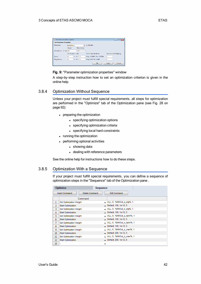
Fig. 9: "Parameter optimization properties" window
A step-by-step instruction how to set an optimization criterion is given in theonline help.
3.8.4 Optimization Without Sequence
Unless your project must fulfill special requirements, all steps for optimizationare performed in the "Optimize" tab of the Optimization pane (see Fig. 28 onpage 92):
l preparing the optimization
l specifying optimization options
l specifying optimization criteria
l specifying local hard constraints
l running the optimization
l performing optional activities
l showing data
l dealing with reference parameters
See the online help for instructions how to do these steps.
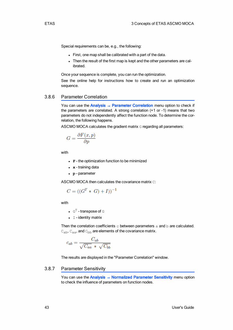
3.8.5 Optimization With a Sequence
If your project must fulfill special requirements, you can define a sequence ofoptimization steps in the "Sequence" tab of the Optimization pane .
ETAS 3Concepts of ETAS ASCMOMOCA
43 User's Guide
Special requirements can be, e.g., the following:
l First, onemap shall be calibrated with a part of the data.
l Then the result of the first map is kept and the other parameters are cal-ibrated.
Once your sequence is complete, you can run the optimization.
See the online help for instructions how to create and run an optimizationsequence.
3.8.6 Parameter Correlation
You can use the Analysis → Parameter Correlation menu option to check ifthe parameters are correlated. A strong correlation (+1 or -1) means that twoparameters do not independently affect the function node. To determine the cor-relation, the following happens.
ASCMOMOCA calculates the gradient matrix G regarding all parameters:
with
l F - the optimization function to beminimized
l x - training data
l p - parameter
ASCMOMOCA then calculates the covariancematrix C:
with
l GT - transpose of G
l I - identity matrix
Then the correlation coefficients c between parameters a and b are calculated.Cab, Caa, and Cbb are elements of the covariancematrix.
The results are displayed in the "Parameter Correlation" window.
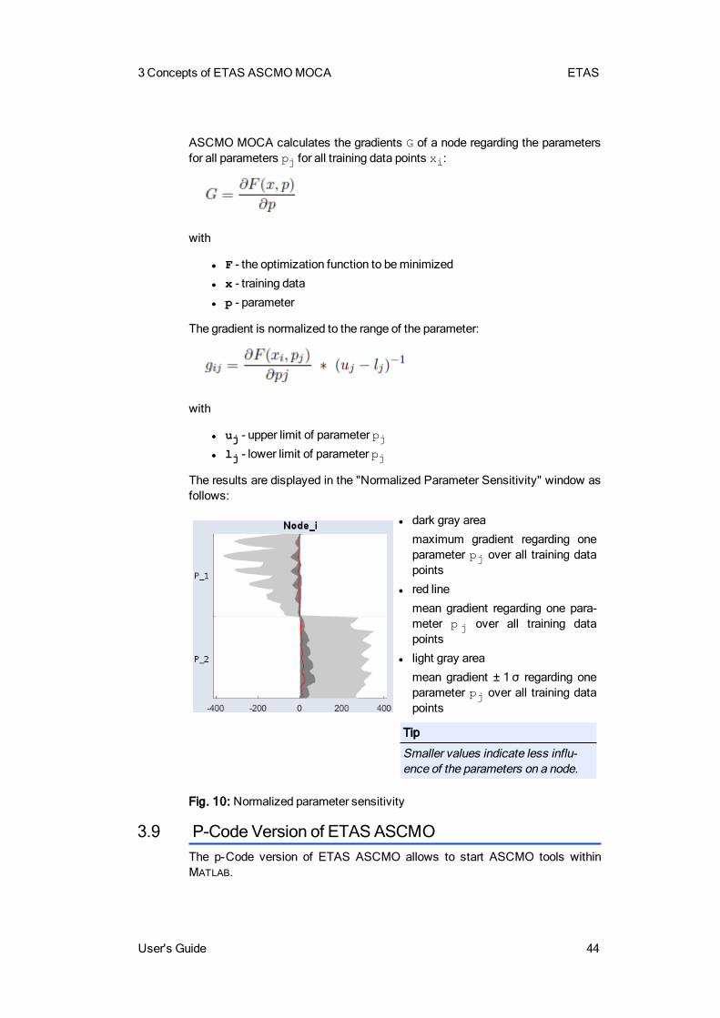
3.8.7 Parameter Sensitivity
You can use the Analysis → Normalized Parameter Sensitivity menu optionto check the influence of parameters on function nodes.
3 Concepts of ETAS ASCMOMOCA ETAS
User's Guide 44
ASCMO MOCA calculates the gradients G of a node regarding the parametersfor all parameters pj for all training data points xi:
with
l F - the optimization function to beminimized
l x - training data
l p - parameter
The gradient is normalized to the range of the parameter:
with
l uj - upper limit of parameter pjl lj - lower limit of parameter pj
The results are displayed in the "Normalized Parameter Sensitivity" window asfollows:
l dark gray area
maximum gradient regarding oneparameter pj over all training datapoints
l red line
mean gradient regarding one para-meter p j over all training datapoints
l light gray area
mean gradient ± 1 σ regarding oneparameter pj over all training datapoints
Tip
Smaller values indicate less influ-ence of the parameters on a node.
Fig. 10: Normalized parameter sensitivity
3.9 P-Code Version of ETASASCMOThe p-Code version of ETAS ASCMO allows to start ASCMO tools withinMATLAB.
ETAS 3Concepts of ETAS ASCMOMOCA
45 User's Guide
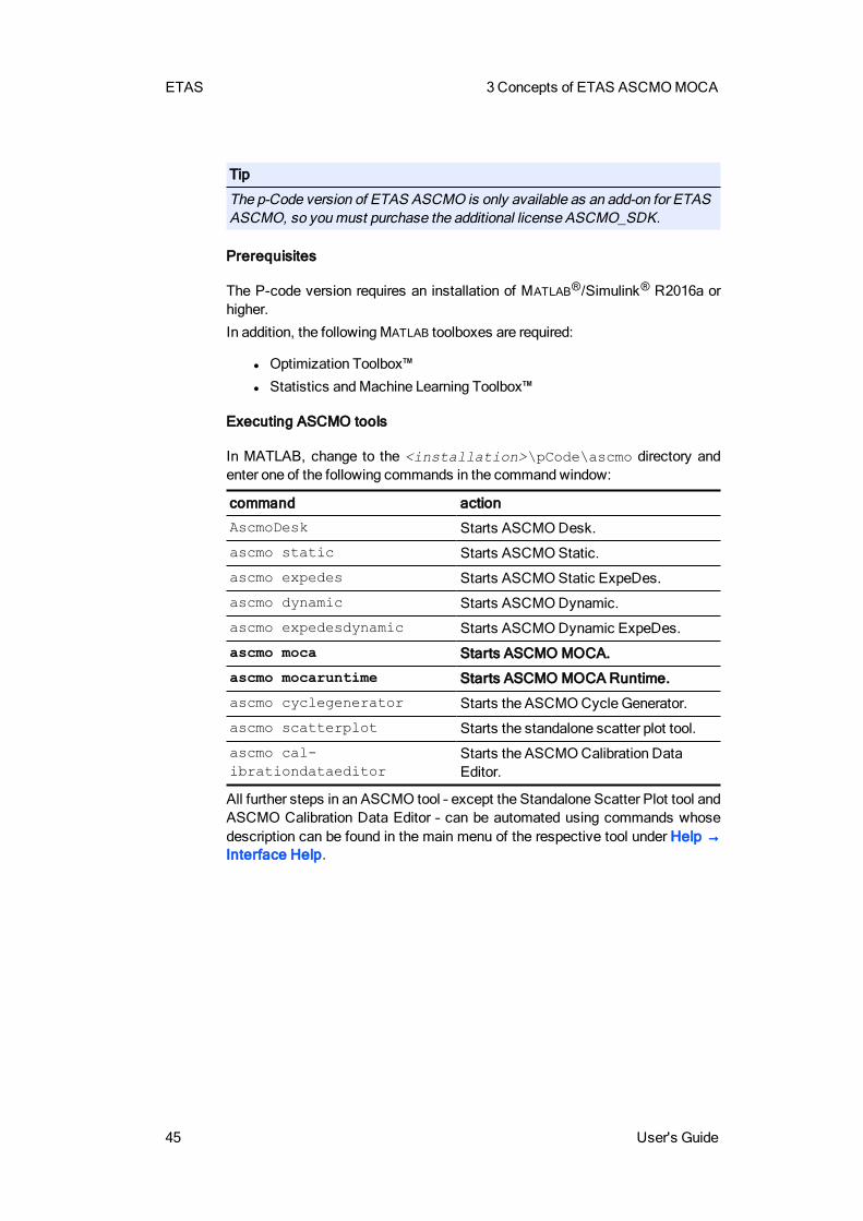
Tip
The p-Code version of ETAS ASCMO is only available as an add-on for ETASASCMO, so youmust purchase the additional license ASCMO_SDK.
Prerequisites
The P-code version requires an installation of MATLAB®/Simulink® R2016a orhigher.
In addition, the followingMATLAB toolboxes are required:
l Optimization Toolbox™
l Statistics andMachine Learning Toolbox™
Executing ASCMO tools
In MATLAB, change to the <installation>\pCode\ascmo directory andenter one of the following commands in the commandwindow:
command action
AscmoDesk Starts ASCMODesk.
ascmo static Starts ASCMOStatic.
ascmo expedes Starts ASCMOStatic ExpeDes.
ascmo dynamic Starts ASCMODynamic.
ascmo expedesdynamic Starts ASCMODynamic ExpeDes.
ascmo moca Starts ASCMO MOCA.
ascmo mocaruntime Starts ASCMO MOCA Runtime.
ascmo cyclegenerator Starts the ASCMOCycle Generator.
ascmo scatterplot Starts the standalone scatter plot tool.
ascmo cal-ibrationdataeditor
Starts the ASCMOCalibration DataEditor.
All further steps in an ASCMO tool – except the Standalone Scatter Plot tool andASCMO Calibration Data Editor – can be automated using commands whosedescription can be found in the main menu of the respective tool under Help →Interface Help.
4 Tutorial: Working with ASCMOMOCA ETAS
User's Guide 46
4 Tutorial: Working with ASCMO MOCAThis chapter will help you with an example to familiarize yourself with the basicfunctions of ETAS ASCMOMOCA.
4.1 About this TutorialIn this section you can find information about the structure of the tutorial andabout the requirements on the measurement data that are used for the para-meter optimization.
4.1.1 Challenge in this Tutorial
An ECU often contains models for the calculation of signals, as the sensor-based data logging is either too difficult or too expensive. A common use caseis, for example, the calculation of the engine torque. With ASCMO MOCA youcan set up and calibrate a function and optimize the function's parametersbased on themeasured sensor data. The goal of the optimizer is to minimize theroot mean square error (see "RMSE (Root Mean Squared Error)" on page 29) ofthe function's parameter. That means that the deviation between the functionprediction and themeasured sensor data will beminimized.
The structure of the torque related function, that will be modeled step by stepduring the tutorial, is displayed in "Step 4: Build Up the Function" on page 82.
4.1.2 Structure of the Tutorial
The subsequent tutorial is structured with the following working steps:
l "Start ASCMO MOCA" auf Seite 48
This part of the tutorial describes how to start ASCMO MOCA on yoursystem.
l "Step 1: Data Import" auf Seite 49
In this first step, the measurement data will first of all be loaded and thechannels will be associated with a function node.
l "Step 2: Data Analysis" auf Seite 65
For clearing up and evaluating the measuring data, at any time, you havethe possibility to visualize it after the import graphically for anytime.
l "Step 3: Models" auf Seite 71
In this step, you are able to link an existing Simulink model with and pre-pare themapping of the parameters, the inputs and outputs.
l "Step 4: Build Up the Function" auf Seite 82
After reading themeasuring data and check the plausibility, you can startto set up the function for the torque sensor that will bemodeled during thetutorial.
l "Step 5: Parameters" auf Seite 91
ETAS 4 Tutorial: Working with ASCMOMOCA
47 User's Guide
This step allows you to check and possibly adapt the parameters. Onlythe parameters will be visualized, which you have defined as referenceafter an optimization (see "Step 6: Optimization" on page 92).
l "Step 6: Optimization" auf Seite 92
Before starting with the optimization you have to insert different settings,which influence the optimization. After you have inserted these settings,you can finally start the optimization.
l "Step 7: Export " auf Seite 95
In this step you will export the created and optimized parameters. Theparameters can be exported as DCM file (*.dcm) and the project can besaved for the runtime environment with limited functionality.
4.1.3 Requirements on Measurement Data
Basically, a simple rule needs to be considered for a successful parameteroptimization in ASCMO MOCA: The quality of the function's parameter optim-ization result always depends on the quality of the measurement data. Or inother words: If the parameters have been calibrated based on non space-fillingor even wrong data, the function prediction is of little use.
Importing the measurement file in ASCMO MOCA requires a file with the fol-lowing properties:
l Data format:
Microsoft Excel (*.xls / *.xlsx)
MDA Export (*.ascii)
CommaSeparated Values (*.csv / *.txt)
Measurement Data Format (*.dat / *.mf4 / *.mdf / *.mdf3)
l Outputs in columns
l Names (and perhaps the units) have to be inserted in the first row ( or inthe first and second row).
Tip
The data used for parameterization do not necessarily have to be derived froma physical experiment (e.g. test bench). They can also be for example a resultof a computer simulation.
4.1.4 Data for Modeling
The data used for the parameter optimization in this tutorial can be found in theTorque_Data.xlsx Excel sheet in the <installation>\Example dir-ectory.
<installation> is the installation directory. By default, <installation>= C:\Programs\ETAS\MOCA 5.4.
The measurement data from this file meets the already mentioned requirementsfor a successful parameter optimization in ASCMOMOCA:

4 Tutorial: Working with ASCMOMOCA ETAS
User's Guide 48
l The experimental design for logging the sensor data (e.g. at a test bench)corresponds to the DoE method, i. e. themeasurements have been var-ied independently and are space-filling.
l Themeasured sensor data from themeasurement file does not includeany absurd values (e.g. values ≤ 0 for torque).
4.2 Start ASCMO MOCAThis part of the tutorial describes how to start ETAS ASCMO MOCA on yoursystem. To do so, proceed as follows.
Starting ASCMO MOCA
1. Do one of the following:
In the ASCMODesk window, click on theModel Calibration tile.
In theWindows start menu, go to theASCMOMOCA V5.4 program group andselect ASCMO MOCA V5.4.
The start window of ASCMOMOCA opens.
Fig. 11: ETAS ASCMOMOCA start window
2. Click on Start MOCA.
The empty main window of ASCMOMOCAopens. Now you can start with themeasurementdata import; see section "Step 1: Data Import" onpage 49.
ETAS 4 Tutorial: Working with ASCMOMOCA
49 User's Guide
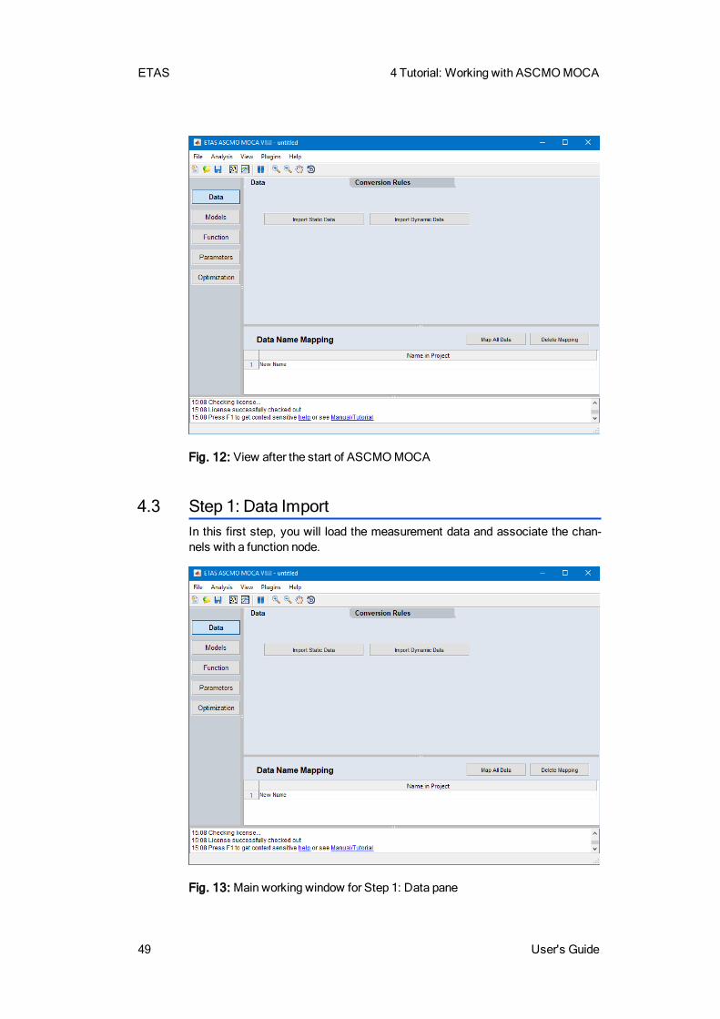
Fig. 12: View after the start of ASCMOMOCA
4.3 Step 1: Data ImportIn this first step, you will load the measurement data and associate the chan-nels with a function node.
Fig. 13: Main working window for Step 1: Data pane
4 Tutorial: Working with ASCMOMOCA ETAS
User's Guide 50
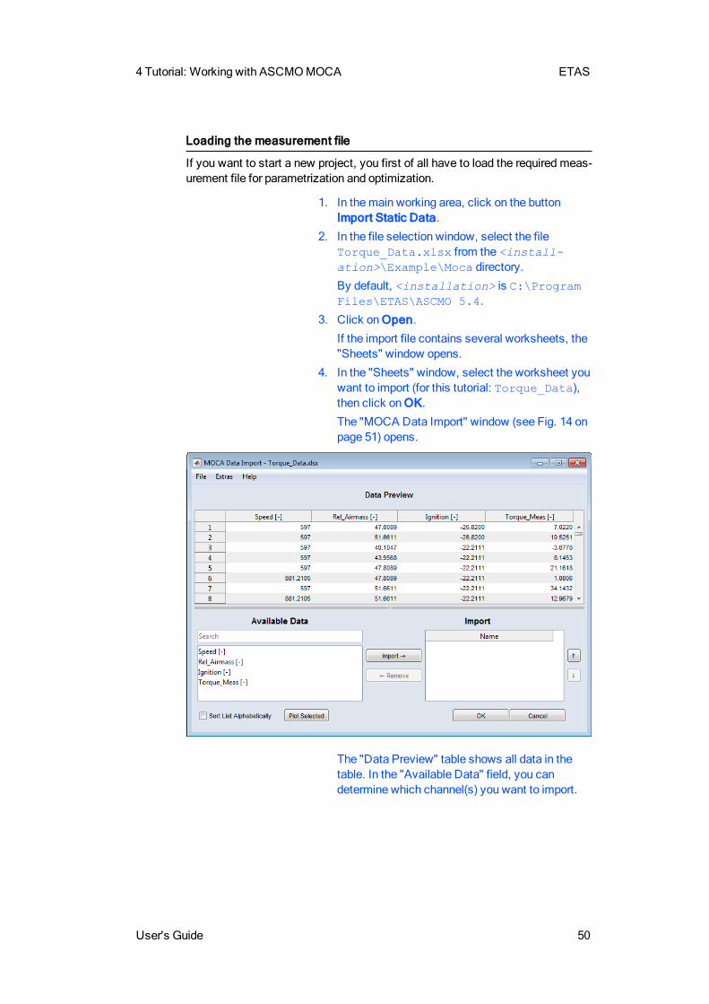
Loading the measurement file
If you want to start a new project, you first of all have to load the required meas-urement file for parametrization and optimization.
1. In themain working area, click on the buttonImport Static Data.
2. In the file selection window, select the fileTorque_Data.xlsx from the <install-ation>\Example\Moca directory.
By default, <installation> is C:\ProgramFiles\ETAS\ASCMO 5.4.
3. Click onOpen.
If the import file contains several worksheets, the"Sheets" window opens.
4. In the "Sheets" window, select the worksheet youwant to import (for this tutorial: Torque_Data),then click onOK.
The "MOCA Data Import" window (see Fig. 14 onpage 51) opens.
The "Data Preview" table shows all data in thetable. In the "Available Data" field, you candetermine which channel(s) you want to import.
ETAS 4 Tutorial: Working with ASCMOMOCA
51 User's Guide
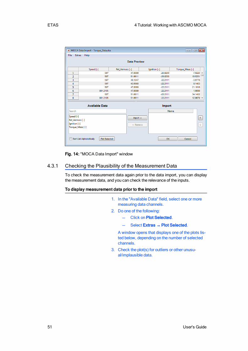
Fig. 14: "MOCA Data Import" window
4.3.1 Checking the Plausibility of the Measurement Data
To check the measurement data again prior to the data import, you can displaythemeasurement data, and you can check the relevance of the inputs.
To display measurement data prior to the import
1. In the "Available Data" field, select one or moremeasuring data channels.
2. Do one of the following:
Click on Plot Selected.
Select Extras → Plot Selected.
A window opens that displays one of the plots lis-ted below, depending on the number of selectedchannels.
3. Check the plot(s) for outliers or other unusu-al/implausible data.
4 Tutorial: Working with ASCMOMOCA ETAS
User's Guide 52
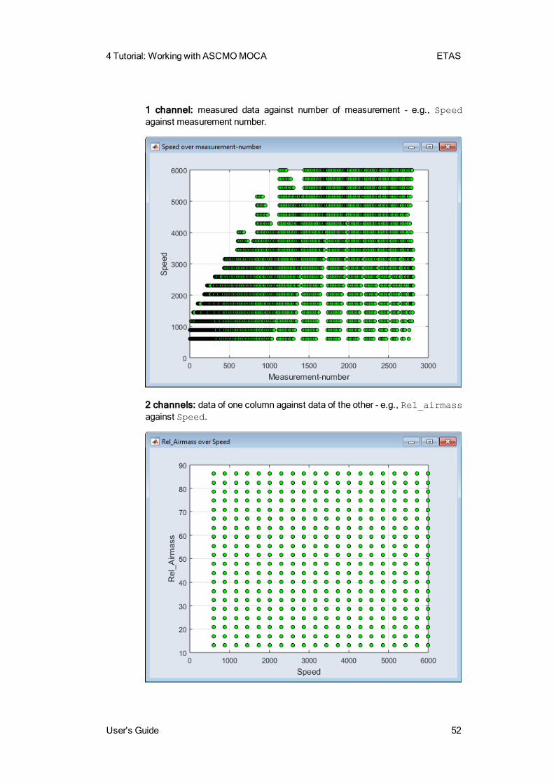
1 channel: measured data against number of measurement - e.g., Speedagainst measurement number.
2 channels: data of one column against data of the other - e.g., Rel_airmassagainst Speed.
ETAS 4 Tutorial: Working with ASCMOMOCA
53 User's Guide
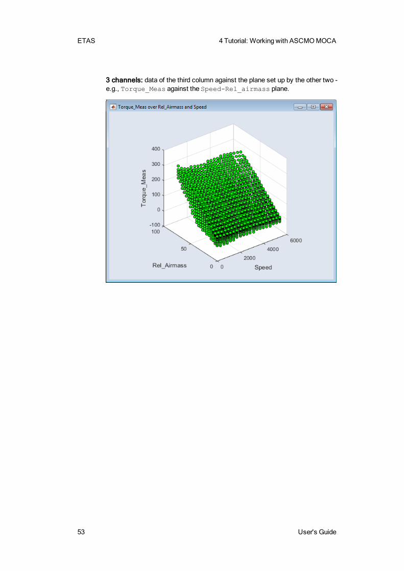
3 channels: data of the third column against the plane set up by the other two -e.g., Torque_Meas against the Speed-Rel_airmass plane.
4 Tutorial: Working with ASCMOMOCA ETAS
User's Guide 54
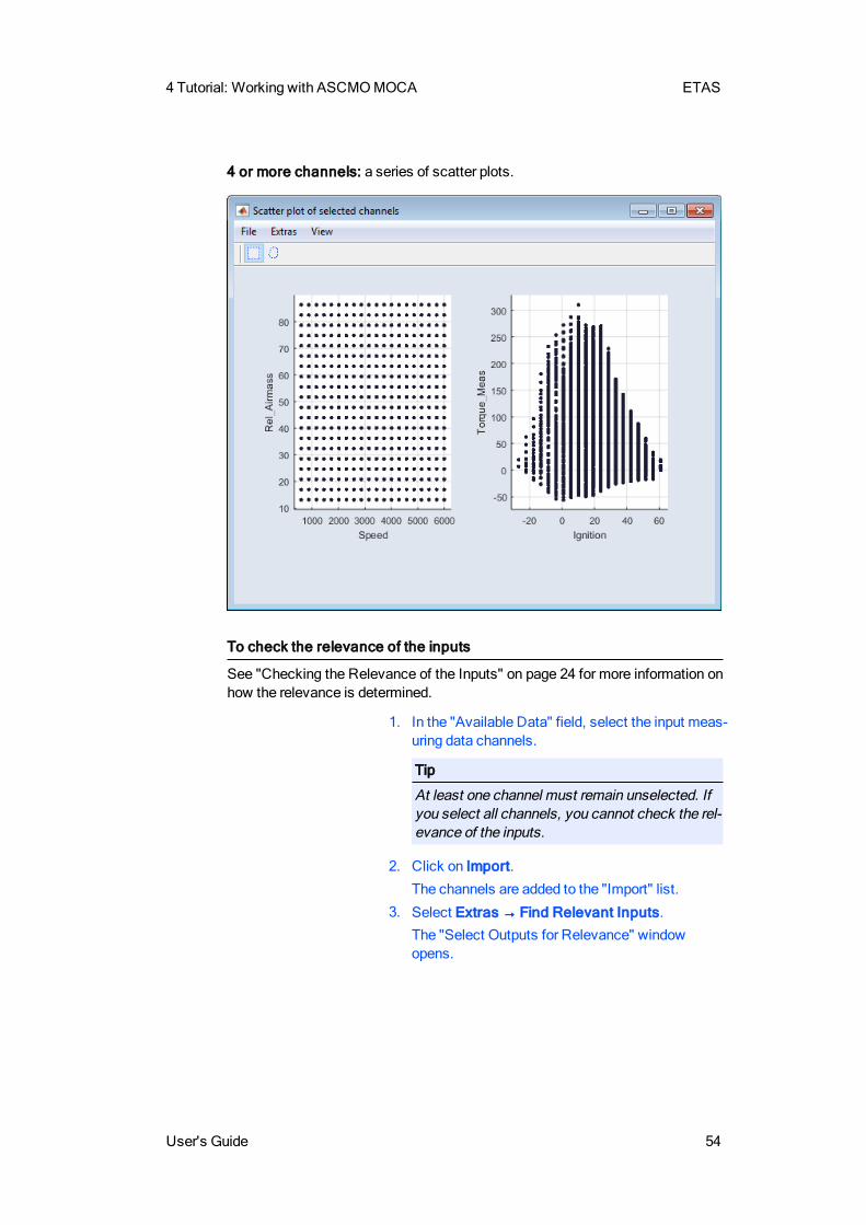
4 or more channels: a series of scatter plots.
To check the relevance of the inputs
See "Checking the Relevance of the Inputs" on page 24 for more information onhow the relevance is determined.
1. In the "Available Data" field, select the input meas-uring data channels.
Tip
At least one channel must remain unselected. Ifyou select all channels, you cannot check the rel-evance of the inputs.
2. Click on Import.
The channels are added to the "Import" list.
3. Select Extras → Find Relevant Inputs.The "Select Outputs for Relevance" windowopens.
ETAS 4 Tutorial: Working with ASCMOMOCA
55 User's Guide
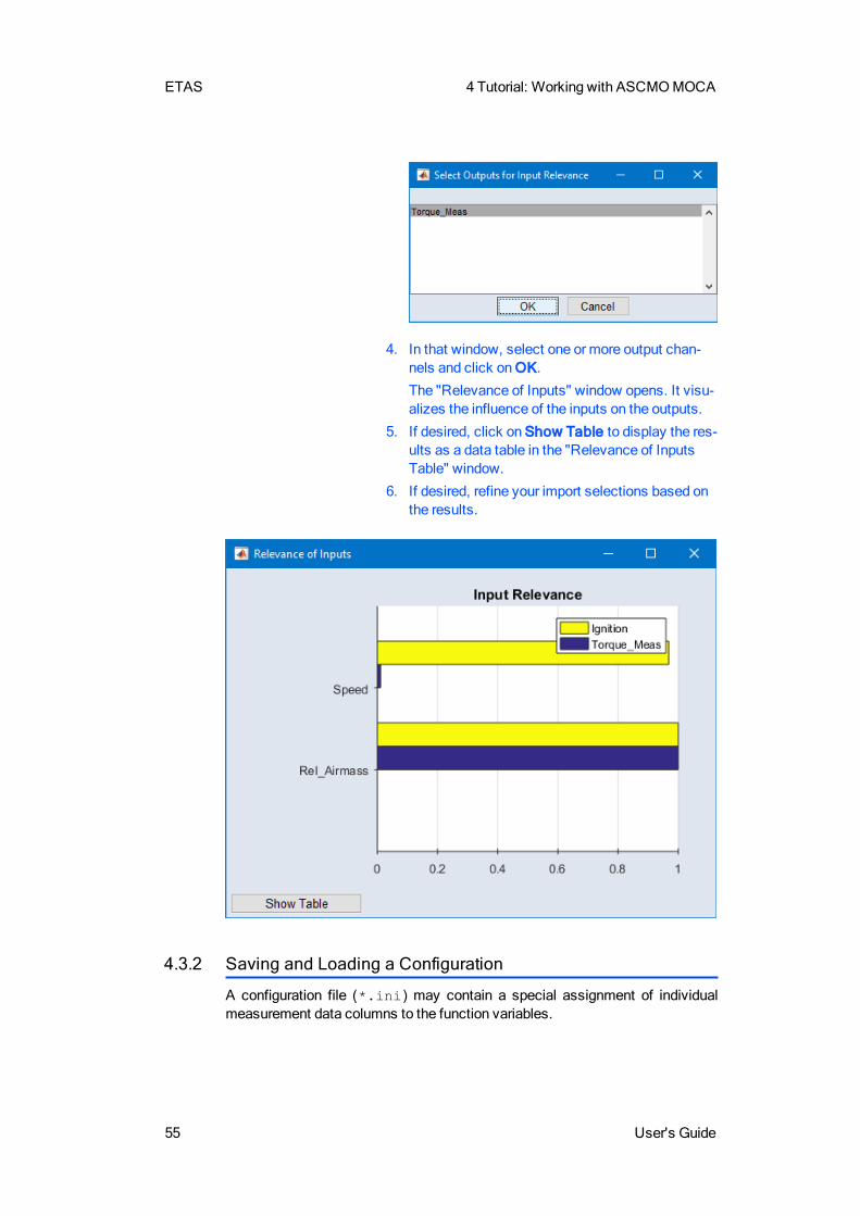
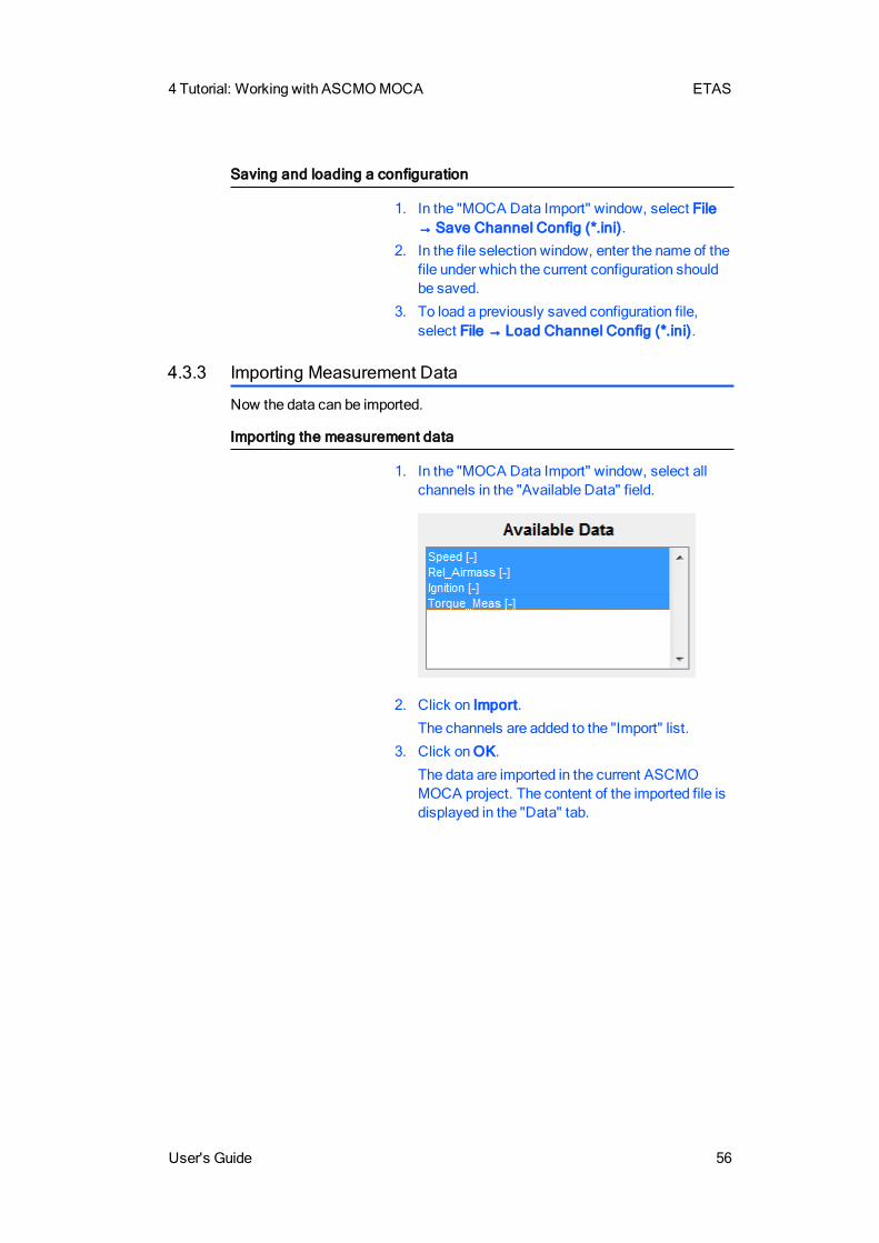
4. In that window, select one or more output chan-nels and click onOK.
The "Relevance of Inputs" window opens. It visu-alizes the influence of the inputs on the outputs.
5. If desired, click on Show Table to display the res-ults as a data table in the "Relevance of InputsTable" window.
6. If desired, refine your import selections based onthe results.
4.3.2 Saving and Loading a Configuration
A configuration file (*.ini) may contain a special assignment of individualmeasurement data columns to the function variables.
4 Tutorial: Working with ASCMOMOCA ETAS
User's Guide 56
Saving and loading a configuration
1. In the "MOCA Data Import" window, select File→ Save Channel Config (*.ini).
2. In the file selection window, enter the name of thefile under which the current configuration shouldbe saved.
3. To load a previously saved configuration file,select File → Load Channel Config (*.ini).
4.3.3 Importing Measurement Data
Now the data can be imported.
Importing the measurement data
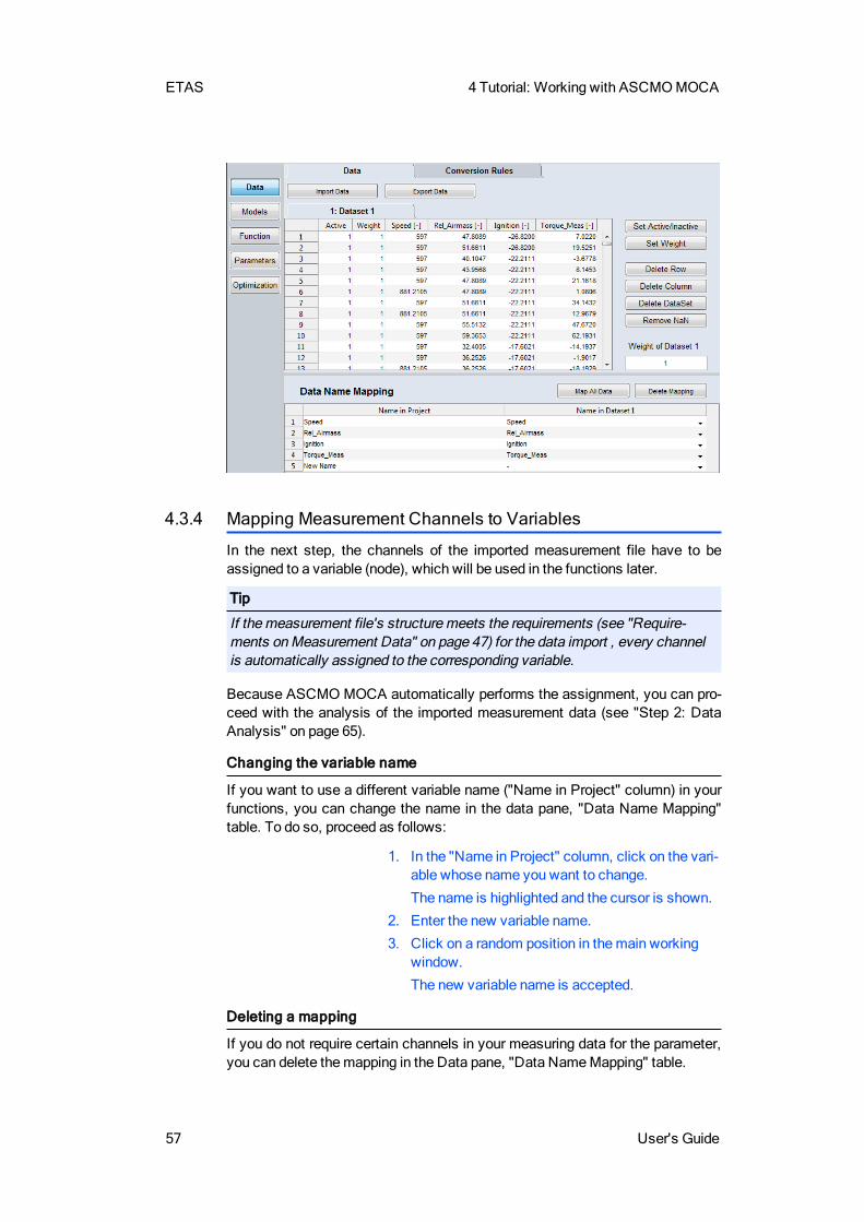
1. In the "MOCA Data Import" window, select allchannels in the "Available Data" field.
2. Click on Import.
The channels are added to the "Import" list.
3. Click onOK.
The data are imported in the current ASCMOMOCA project. The content of the imported file isdisplayed in the "Data" tab.
ETAS 4 Tutorial: Working with ASCMOMOCA
57 User's Guide
4.3.4 Mapping Measurement Channels to Variables
In the next step, the channels of the imported measurement file have to beassigned to a variable (node), which will be used in the functions later.
Tip
If themeasurement file's structuremeets the requirements (see "Require-ments onMeasurement Data" on page 47) for the data import , every channelis automatically assigned to the corresponding variable.
Because ASCMO MOCA automatically performs the assignment, you can pro-ceed with the analysis of the imported measurement data (see "Step 2: DataAnalysis" on page 65).
Changing the variable name
If you want to use a different variable name ("Name in Project" column) in yourfunctions, you can change the name in the data pane, "Data Name Mapping"table. To do so, proceed as follows:
1. In the "Name in Project" column, click on the vari-able whose name you want to change.
The name is highlighted and the cursor is shown.
2. Enter the new variable name.
3. Click on a random position in themain workingwindow.
The new variable name is accepted.
Deleting a mapping
If you do not require certain channels in your measuring data for the parameter,you can delete themapping in the Data pane, "Data NameMapping" table.
4 Tutorial: Working with ASCMOMOCA ETAS
User's Guide 58
1. In the "Name in Function" column, select thedesired variable.
2. Click on Delete Mapping.
The variable is deleted from the "Data NameMap-ping" table.
4.3.5 Working in the Data Pane of ASCMOMOCA
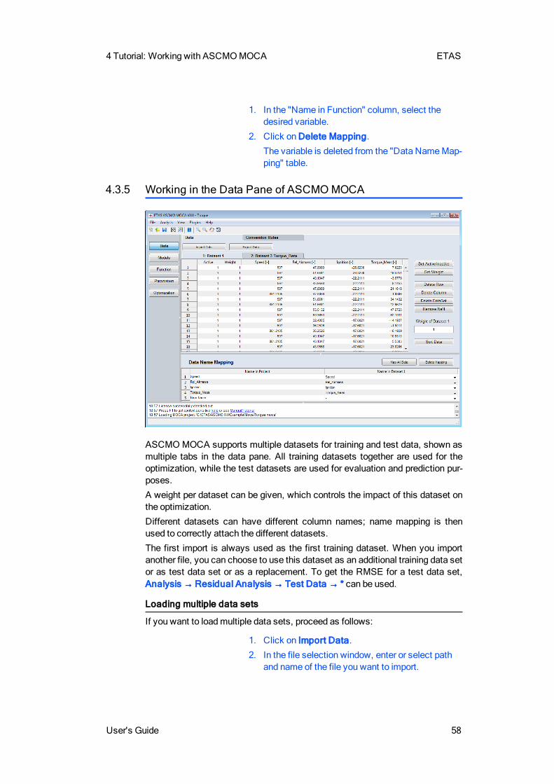
ASCMOMOCA supports multiple datasets for training and test data, shown asmultiple tabs in the data pane. All training datasets together are used for theoptimization, while the test datasets are used for evaluation and prediction pur-poses.
A weight per dataset can be given, which controls the impact of this dataset onthe optimization.
Different datasets can have different column names; name mapping is thenused to correctly attach the different datasets.
The first import is always used as the first training dataset. When you importanother file, you can choose to use this dataset as an additional training data setor as test data set or as a replacement. To get the RMSE for a test data set,Analysis → Residual Analysis → Test Data → * can be used.
Loading multiple data sets
If you want to loadmultiple data sets, proceed as follows:
1. Click on Import Data.
2. In the file selection window, enter or select pathand name of the file you want to import.
ETAS 4 Tutorial: Working with ASCMOMOCA
59 User's Guide
Allowed file formats are *.xls, *.xlsx, *.csvand *.txt.
3. Click onOpen.
The "MOCA Data Import - <file name>" windowopens.
4. In that window, select the input channels asdescribed in "Loading themeasurement file" onpage 50.
5. Click onOK.
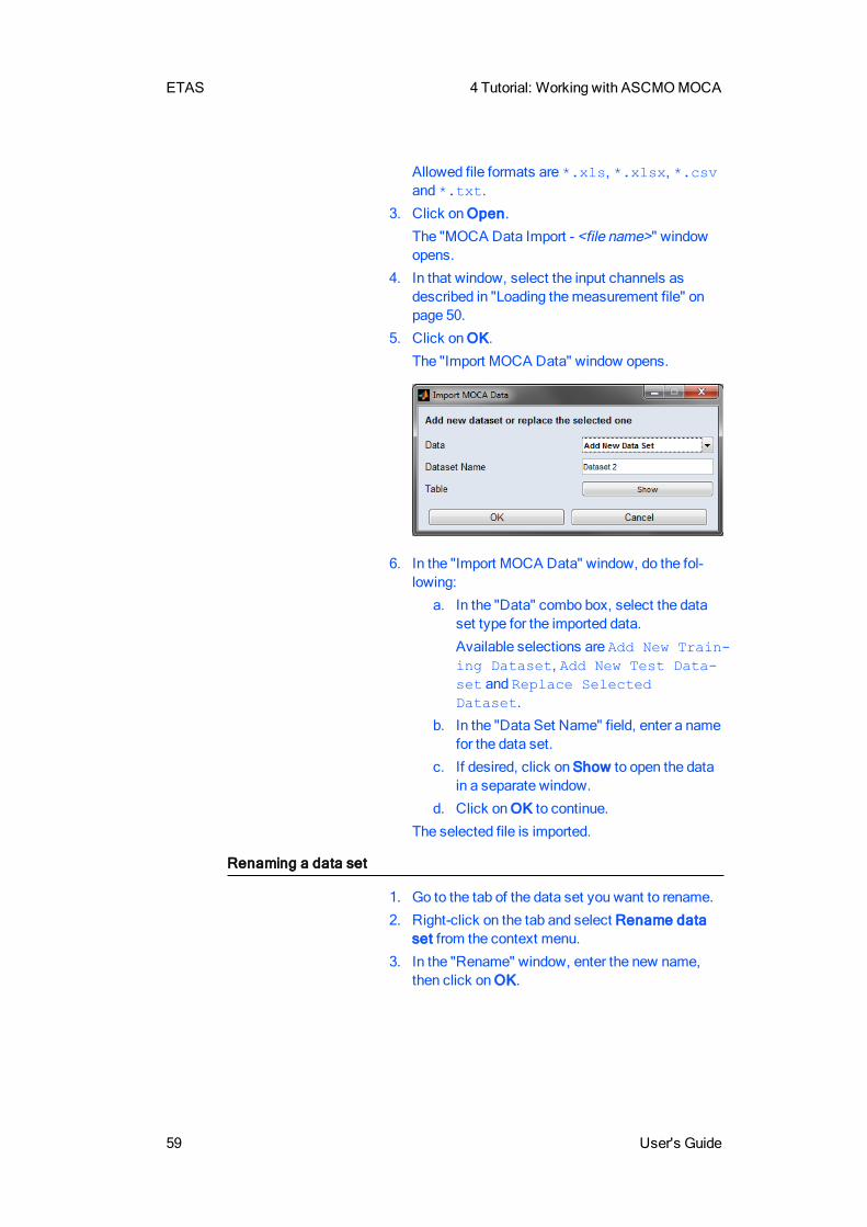
The "Import MOCA Data" window opens.
6. In the "Import MOCA Data" window, do the fol-lowing:
a. In the "Data" combo box, select the dataset type for the imported data.
Available selections are Add New Train-ing Dataset, Add New Test Data-set and Replace SelectedDataset.
b. In the "Data Set Name" field, enter a namefor the data set.
c. If desired, click on Show to open the datain a separate window.
d. Click onOK to continue.
The selected file is imported.
Renaming a data set
1. Go to the tab of the data set you want to rename.
2. Right-click on the tab and select Rename dataset from the context menu.
3. In the "Rename" window, enter the new name,then click onOK.
4 Tutorial: Working with ASCMOMOCA ETAS
User's Guide 60
Deleting a data set
1. Go to the tab of the data set you want to delete.
2. Click on Delete Dataset.
A confirmation window opens.
3. In the confirmation window, click on Delete.
The selected data set is deleted from the project.
Data Point ActivationWith the "Active" column, rows of data can be set inactive by setting the valueto zero. Inactive rows are ignored for the RMSE calculation and optimization.
Multiple rows can be selected with the <SHIFT> key and left mouse button click-ing. Then, the selected rows can be set inactive with the Set Active/Inactivebutton .
Another possibility to activate/deactivate data points is available in the scatterplot window, opened with Analysis → Scatter Plot → *. After marking somedata points in a scatter plot, you can use the Extras → Set Marked Points Act-ive and Inactive menu options to activate/deactivate themarked data points.
Activating/deactivating data points
1. To activate/deactivate data points via the Set Act-ive/Inactive button, proceed as follows:
a. In the "Active" column, select one or morerows.
b. Click on Set Active/Inactive.
If the value in the "Active" columnwas 1, itchanges to 0 (inactive).
If the value in the "Active" columnwas 0, itchanges to 1 (active).
2. To activate/deactivate an individual data point,proceed as follows:
a. In the "Active" column, click in the row youwant to edit.
b. To deactivate the row, enter 0.
c. To activate the row, enter 1.
Tip
Any value ≠ 0 (including negative numbers andarbitrary characters) is interpreted as active.

ETAS 4 Tutorial: Working with ASCMOMOCA
61 User's Guide
Data Point WeightsWith the "Weight" column, the optimization weight for a data point can be set.The default is one and higher values show the optimizer that the respectivepoints are more important, i.e. a stronger emphasis to meet the optimization cri-terion for this data point. The weight influences the optimization but is not reflec-ted in the displayed RMSE.
Multiple rows can be selected with the <SHIFT> and <CTRL> key and leftmouse button clicking. Then the weight for multiple rows can be set with the SetWeight button.
Another possibility to set the weight of data points is available in the scatter plotwindow, opened with Analysis → Scatter Plot → *. After marking some datapoints in a scatter plot, you can use the Extras → Set Marked Points Weightmenu option to set the weight for themarked data.
Setting the weights of selected data points
1. To set the weights of data points via the SetWeight button, proceed as follows:
a. Select one or more rows.
b. Click on Set Weight.
c. In the "DataWeights" window, enter theweight for the selected rows.
d. Click onOK.
The weight is assigned to all selectedrows.
2. To set the weight of an individual row, proceed asfollows:
a. In the "Weight" column, click in the rowyou want to edit.
b. Enter the number you want to assign.
Adjusting the weights of the entire data set
To adjust the weights of the entire data set, proceed as follows:
Tip
The data set weight has no effect if there is just one data set.
4 Tutorial: Working with ASCMOMOCA ETAS
User's Guide 62
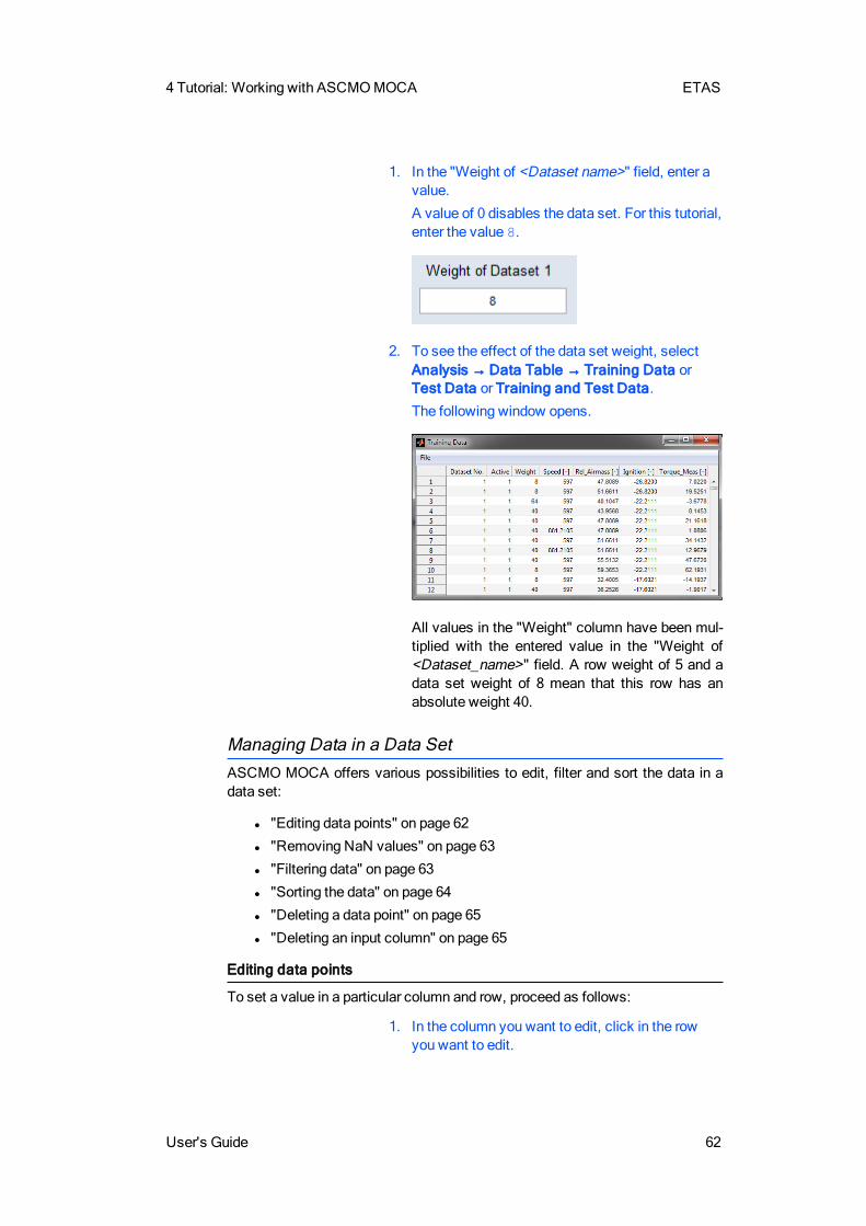
1. In the "Weight of <Dataset name>" field, enter avalue.
A value of 0 disables the data set. For this tutorial,enter the value 8.
2. To see the effect of the data set weight, selectAnalysis → Data Table → Training Data orTest Data or Training and Test Data.
The following window opens.
All values in the "Weight" column have been mul-tiplied with the entered value in the "Weight of<Dataset_name>" field. A row weight of 5 and adata set weight of 8 mean that this row has anabsolute weight 40.
Managing Data in a Data SetASCMO MOCA offers various possibilities to edit, filter and sort the data in adata set:
l "Editing data points" on page 62
l "Removing NaN values" on page 63
l "Filtering data" on page 63
l "Sorting the data" on page 64
l "Deleting a data point" on page 65
l "Deleting an input column" on page 65
Editing data points
To set a value in a particular column and row, proceed as follows:
1. In the column you want to edit, click in the rowyou want to edit.
ETAS 4 Tutorial: Working with ASCMOMOCA
63 User's Guide
2. Enter the number you want to assign.
Removing NaN values
If your imported data contains non-numeric values, you can automatically deletethe affected rows in all data sets. Proceed as follows:
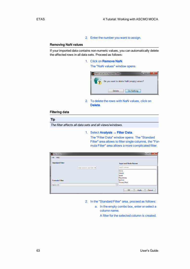
1. Click on Remove NaN.
The "NaN values" window opens.
2. To delete the rows with NaN values, click onDelete.
Filtering data
Tip
The filter affects all data sets and all views/windows.
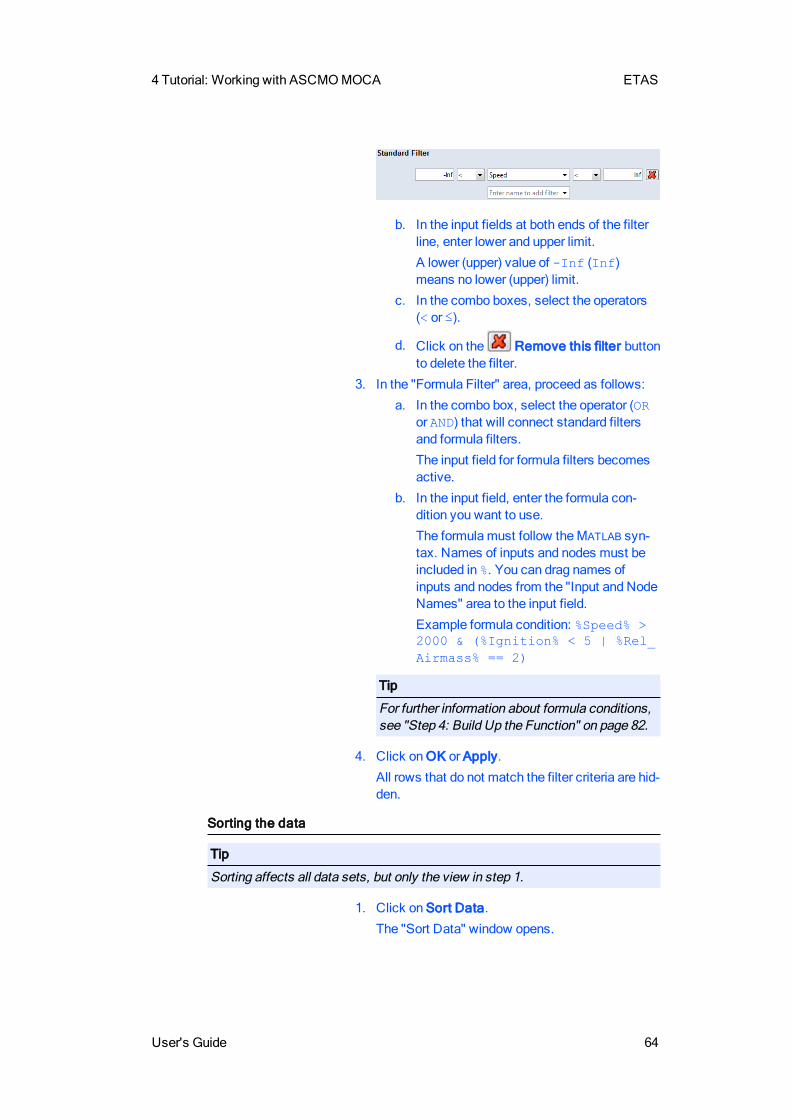
1. Select Analysis → Filter Data.The "Filter Data" window opens. The "StandardFilter" area allows to filter single columns, the "For-mula Filter" area allows amore complicated filter.
2. In the "Standard Filter" area, proceed as follows:
a. In the empty combo box, enter or select acolumn name.
A filter for the selected column is created.
4 Tutorial: Working with ASCMOMOCA ETAS
User's Guide 64
b. In the input fields at both ends of the filterline, enter lower and upper limit.
A lower (upper) value of -Inf (Inf)means no lower (upper) limit.
c. In the combo boxes, select the operators(< or ≤).
d. Click on the Remove this filter buttonto delete the filter.
3. In the "Formula Filter" area, proceed as follows:
a. In the combo box, select the operator (ORor AND) that will connect standard filtersand formula filters.
The input field for formula filters becomesactive.
b. In the input field, enter the formula con-dition you want to use.
The formulamust follow theMATLAB syn-tax. Names of inputs and nodes must beincluded in %. You can drag names ofinputs and nodes from the "Input and NodeNames" area to the input field.
Example formula condition: %Speed% >2000 & (%Ignition% < 5 | %Rel_Airmass% == 2)
Tip
For further information about formula conditions,see "Step 4: Build Up the Function" on page 82.
4. Click onOK or Apply.
All rows that do not match the filter criteria are hid-den.
Sorting the data
Tip
Sorting affects all data sets, but only the view in step 1.
1. Click on Sort Data.
The "Sort Data" window opens.

ETAS 4 Tutorial: Working with ASCMOMOCA
65 User's Guide
2. In the "ColumnName" combo box, select acolumn.
3. Click onOK.
The tables are sorted by the selected column, inascending order.
Deleting a data point
1. Select a value in one or more rows.
2. Click on Delete Row.
A confirmation window opens.
3. In the confirmation window, click on Delete.
The selected rows are deleted.
Deleting an input column
1. Select a value in one or more columns.
2. Click on Delete Column.
A confirmation window opens.
3. In the confirmation window, click on Delete.
The selected columns are deleted.
4.4 Step 2: Data AnalysisFor clearing up and evaluating the measuring data, you have the possibility tovisualize it after the import graphically for anytime.
During the analysis, particular the following points should be considered.
l Have all parameters been varied according to the experiment plan anddid themeasured system remain in the operatingmode intended for thispurpose?
l Do the output variables fall in physically meaningful ranges?
l Are there any outliers included, which have to be removed, if appro-priate?
Visualizing measurement data in a scatter plot
1. Select Analysis → Scatter Plot → *1. →Data/Function Nodes.
1. * = Training Data or Test Data or Training and Test Data
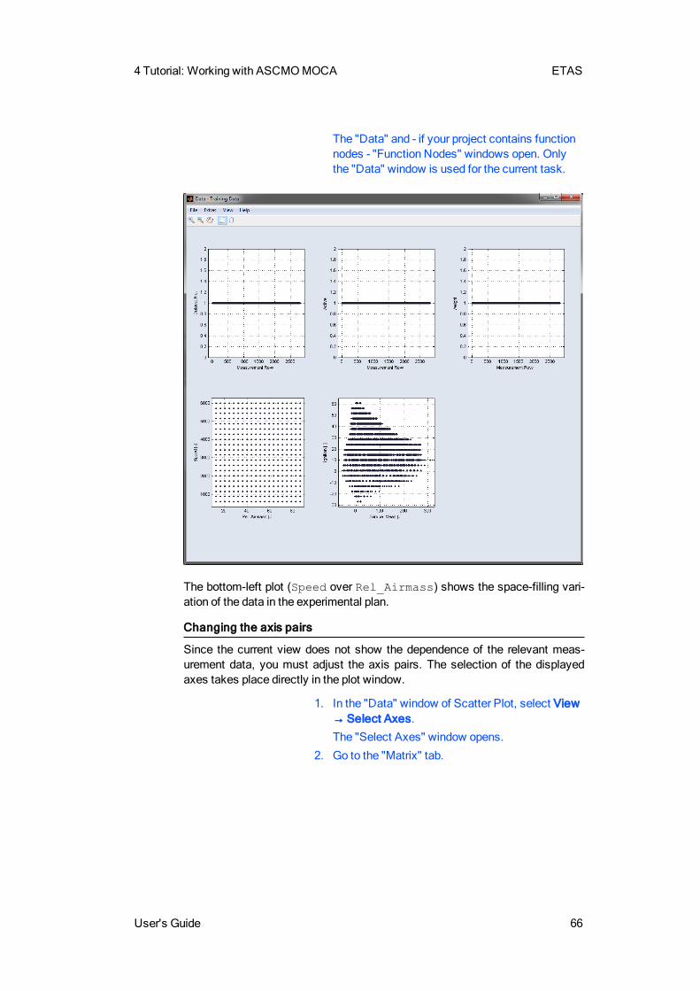
4 Tutorial: Working with ASCMOMOCA ETAS
User's Guide 66
The "Data" and - if your project contains functionnodes - "Function Nodes" windows open. Onlythe "Data" window is used for the current task.
The bottom-left plot (Speed over Rel_Airmass) shows the space-filling vari-ation of the data in the experimental plan.
Changing the axis pairs
Since the current view does not show the dependence of the relevant meas-urement data, you must adjust the axis pairs. The selection of the displayedaxes takes place directly in the plot window.
1. In the "Data" window of Scatter Plot, select View→ Select Axes.The "Select Axes" window opens.
2. Go to the "Matrix" tab.
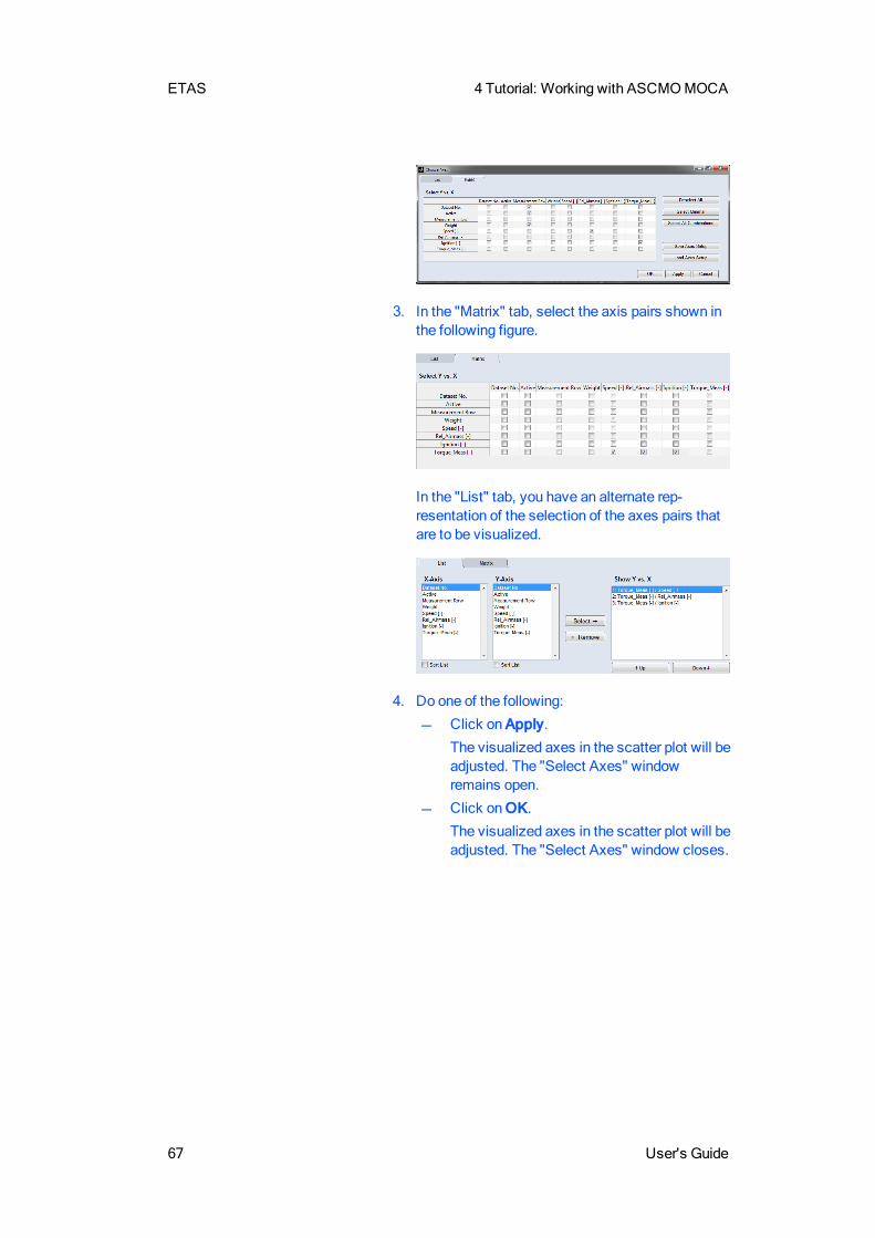
ETAS 4 Tutorial: Working with ASCMOMOCA
67 User's Guide
3. In the "Matrix" tab, select the axis pairs shown inthe following figure.
In the "List" tab, you have an alternate rep-resentation of the selection of the axes pairs thatare to be visualized.
4. Do one of the following:
Click on Apply.
The visualized axes in the scatter plot will beadjusted. The "Select Axes" windowremains open.
Click onOK.
The visualized axes in the scatter plot will beadjusted. The "Select Axes" window closes.

4 Tutorial: Working with ASCMOMOCA ETAS
User's Guide 68
Deleting an outlier
You can now use the scatter plots to remove outliers.
1. Search the plots for outliers.
In this tutorial, use the top-left point in the"Torque_Meas over Speed" plot, with Torque_Meas > 300.
2. Click on the Mouse selection in Plot withRectangle button.
3. Click in the plot and draw a rectangle around theoutlier.
The selected points are colored in all scatter plots.
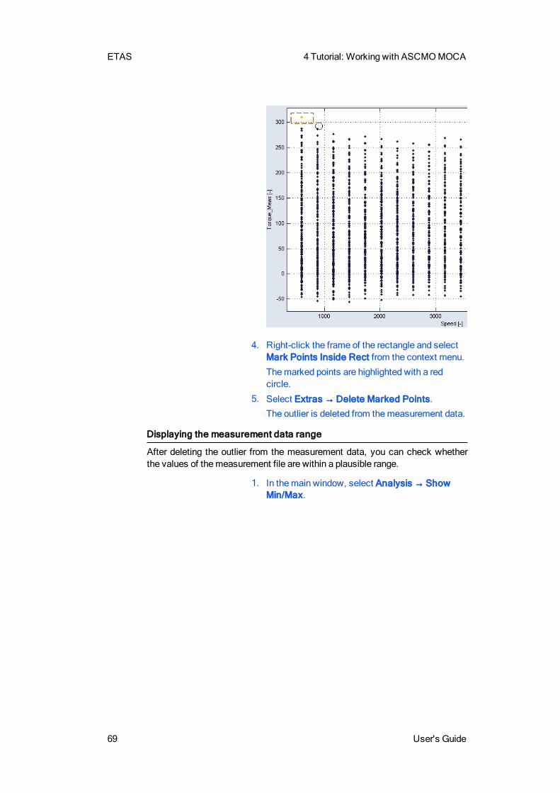
ETAS 4 Tutorial: Working with ASCMOMOCA
69 User's Guide
4. Right-click the frame of the rectangle and selectMark Points Inside Rect from the context menu.
Themarked points are highlighted with a redcircle.
5. Select Extras → Delete Marked Points.The outlier is deleted from themeasurement data.
Displaying the measurement data range
After deleting the outlier from the measurement data, you can check whetherthe values of themeasurement file are within a plausible range.
1. In themain window, select Analysis → ShowMin/Max.

4 Tutorial: Working with ASCMOMOCA ETAS
User's Guide 70
The "Min/Max Data & Nodes" window opens.
After importing and reviewing themeasurement data, you can start to add nodesto the function. To do so, select the Function working step in the navigation(see "Main Elements of the User Interface" on page 20). The respective ele-ments in the main working window will appear, where you can save, delete andedit the function "Step 4: Build Up the Function" on page 82).
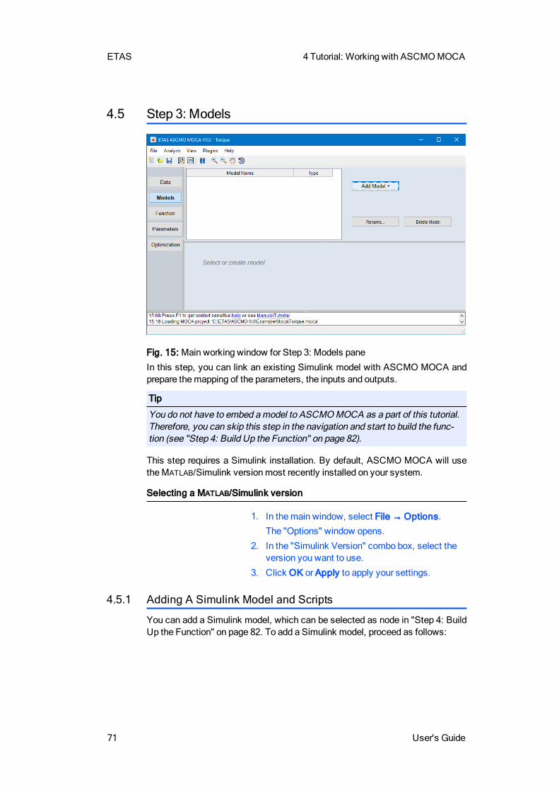
ETAS 4 Tutorial: Working with ASCMOMOCA
71 User's Guide
4.5 Step 3: Models
Fig. 15: Main working window for Step 3: Models pane
In this step, you can link an existing Simulink model with ASCMO MOCA andprepare themapping of the parameters, the inputs and outputs.
Tip
You do not have to embed amodel to ASCMOMOCA as a part of this tutorial.Therefore, you can skip this step in the navigation and start to build the func-tion (see "Step 4: Build Up the Function" on page 82).
This step requires a Simulink installation. By default, ASCMO MOCA will usetheMATLAB/Simulink versionmost recently installed on your system.
Selecting a MATLAB/Simulink version
1. In themain window, select File → Options.The "Options" window opens.
2. In the "Simulink Version" combo box, select theversion you want to use.
3. Click OK or Apply to apply your settings.
4.5.1 Adding A Simulink Model and Scripts
You can add a Simulink model, which can be selected as node in "Step 4: BuildUp the Function" on page 82. To add a Simulink model, proceed as follows:
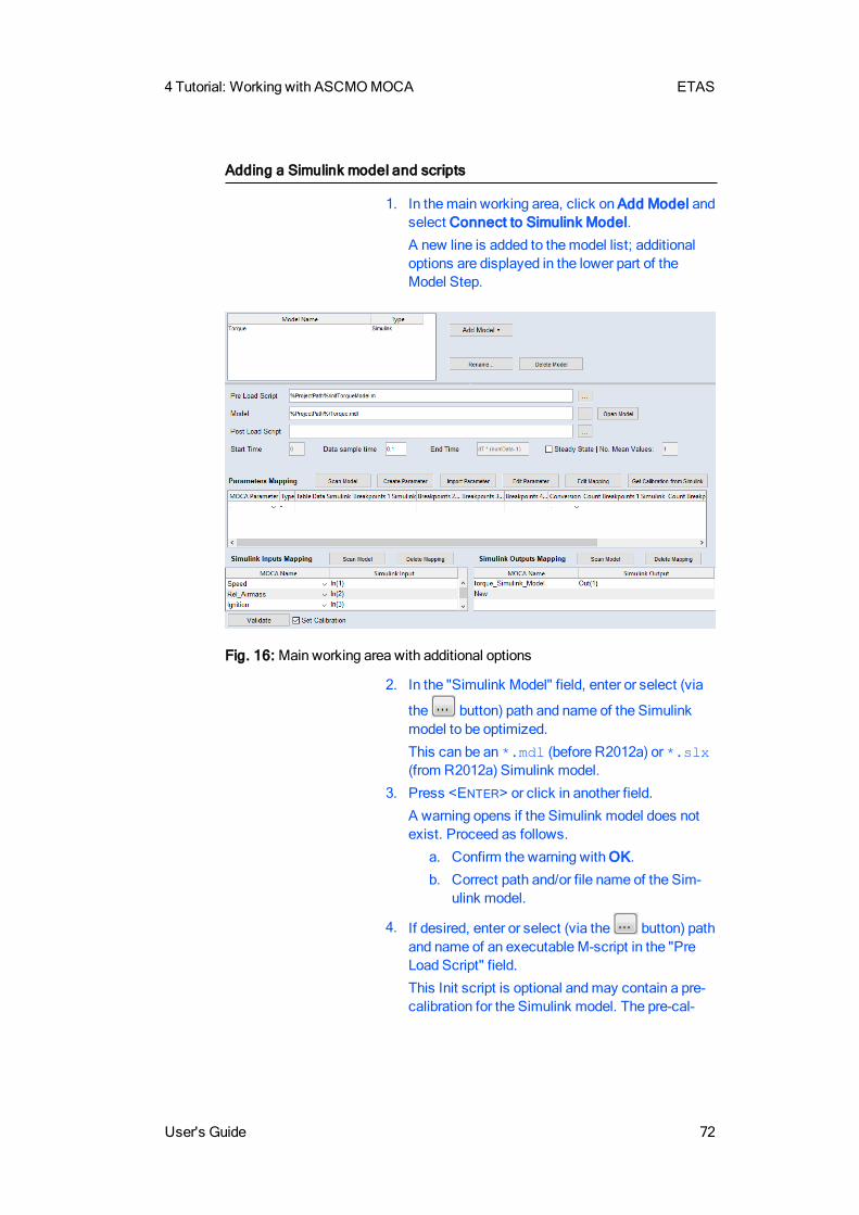
4 Tutorial: Working with ASCMOMOCA ETAS
User's Guide 72
Adding a Simulink model and scripts
1. In themain working area, click on Add Model andselect Connect to Simulink Model.
A new line is added to themodel list; additionaloptions are displayed in the lower part of theModel Step.
Fig. 16: Main working area with additional options
2. In the "Simulink Model" field, enter or select (via
the button) path and name of the Simulinkmodel to be optimized.
This can be an *.mdl (before R2012a) or *.slx(from R2012a) Simulink model.
3. Press <ENTER> or click in another field.
A warning opens if the Simulink model does notexist. Proceed as follows.
a. Confirm the warning with OK.
b. Correct path and/or file name of the Sim-ulink model.
4. If desired, enter or select (via the button) pathand name of an executable M-script in the "PreLoad Script" field.
This Init script is optional andmay contain a pre-calibration for the Simulink model. The pre-cal-
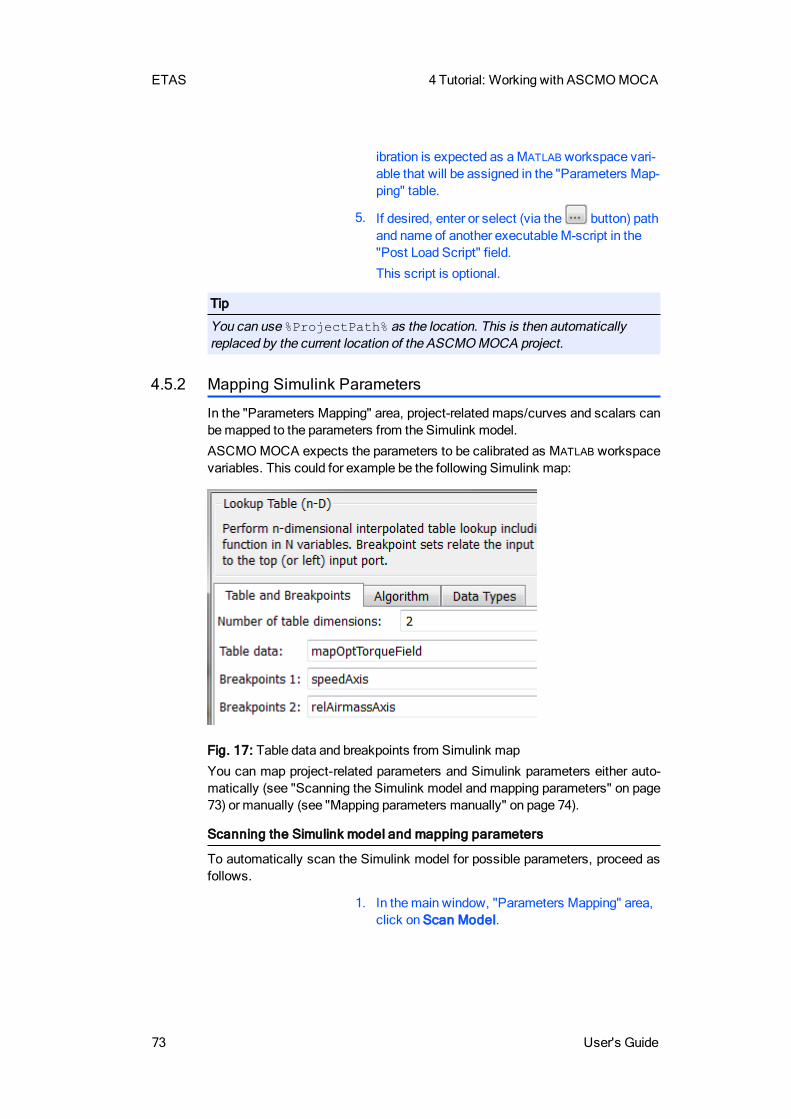
ETAS 4 Tutorial: Working with ASCMOMOCA
73 User's Guide
ibration is expected as aMATLABworkspace vari-able that will be assigned in the "Parameters Map-ping" table.
5. If desired, enter or select (via the button) pathand name of another executable M-script in the"Post Load Script" field.
This script is optional.
Tip
You can use %ProjectPath% as the location. This is then automaticallyreplaced by the current location of the ASCMOMOCA project.
4.5.2 Mapping Simulink Parameters
In the "Parameters Mapping" area, project-related maps/curves and scalars canbemapped to the parameters from the Simulink model.
ASCMOMOCA expects the parameters to be calibrated as MATLAB workspacevariables. This could for example be the following Simulink map:
Fig. 17: Table data and breakpoints from Simulink map
You can map project-related parameters and Simulink parameters either auto-matically (see "Scanning the Simulink model and mapping parameters" on page73) or manually (see "Mapping parameters manually" on page 74).
Scanning the Simulink model and mapping parameters
To automatically scan the Simulink model for possible parameters, proceed asfollows.
1. In themain window, "Parameters Mapping" area,click on Scan Model.

4 Tutorial: Working with ASCMOMOCA ETAS
User's Guide 74
The block masks of lookup tables and otherblocks are scanned for variable names. The res-ults are then presented in the "ScanModel<model_name> for Parameter Mapping" window.
Fig. 18: "ScanModel <model_name> for Parameter Mapping" window
2. Activate/deactivate the Constants, Curvesand/or Maps options to show/hide parameters ofthe respective types.
3. In the "Filter" field, enter the string by which youwant to filter the list, then press <ENTER>.
Tip
The filter is not caps-sensitive. You cannot usewildcards.
Only parameters whose Simulink names or pathscontain the search string are displayed. If youenter the search term Ignition, for example, allrows from Fig. 18 except the third will be hidden.
4. In the "CreateMapping" column, activate theoptions in all rows you want to map.
5. Click on Add Mappings to add the selectedmap-pings to the "Parameters Mapping" list.
With Add Mappings, existing content in the"Parameters Mapping" list is kept. If an existingrow is selected again, this selection is ignored andamessage is issued in the log window.
Replace Mappings removes existing content inthe "Parameters Mapping" list.
Mapping parameters manually
Tomap the parameters manually, proceed as follows:
1. In the "Parameters Mapping" area, "MOCA Para-meter" column, select a parameter from thecombo box.
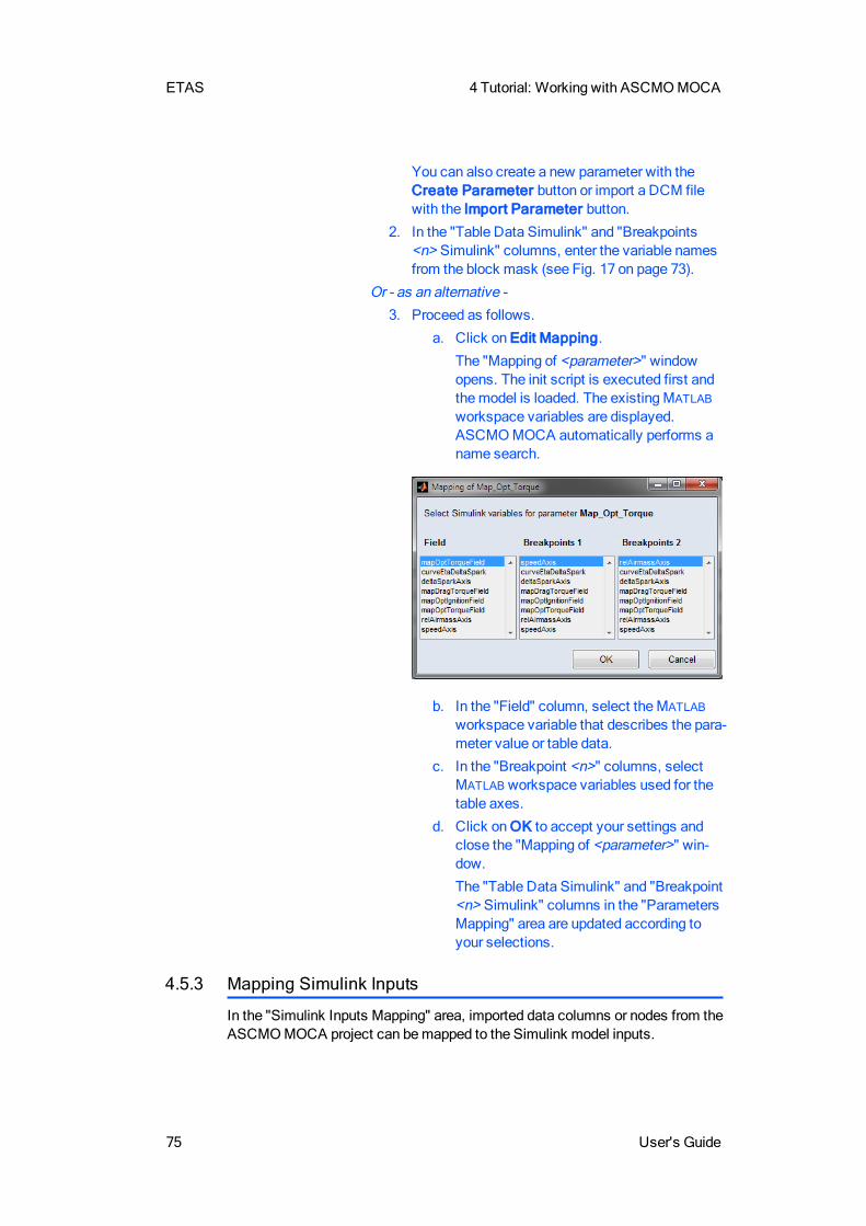
ETAS 4 Tutorial: Working with ASCMOMOCA
75 User's Guide
You can also create a new parameter with theCreate Parameter button or import a DCM filewith the Import Parameter button.
2. In the "Table Data Simulink" and "Breakpoints<n> Simulink" columns, enter the variable namesfrom the block mask (see Fig. 17 on page 73).
Or - as an alternative -3. Proceed as follows.
a. Click on Edit Mapping.
The "Mapping of <parameter>" windowopens. The init script is executed first andthemodel is loaded. The existingMATLAB
workspace variables are displayed.ASCMOMOCA automatically performs aname search.
b. In the "Field" column, select theMATLAB
workspace variable that describes the para-meter value or table data.
c. In the "Breakpoint <n>" columns, selectMATLABworkspace variables used for thetable axes.
d. Click onOK to accept your settings andclose the "Mapping of <parameter>" win-dow.
The "Table Data Simulink" and "Breakpoint<n> Simulink" columns in the "ParametersMapping" area are updated according toyour selections.
4.5.3 Mapping Simulink Inputs
In the "Simulink Inputs Mapping" area, imported data columns or nodes from theASCMOMOCA project can bemapped to the Simulink model inputs.
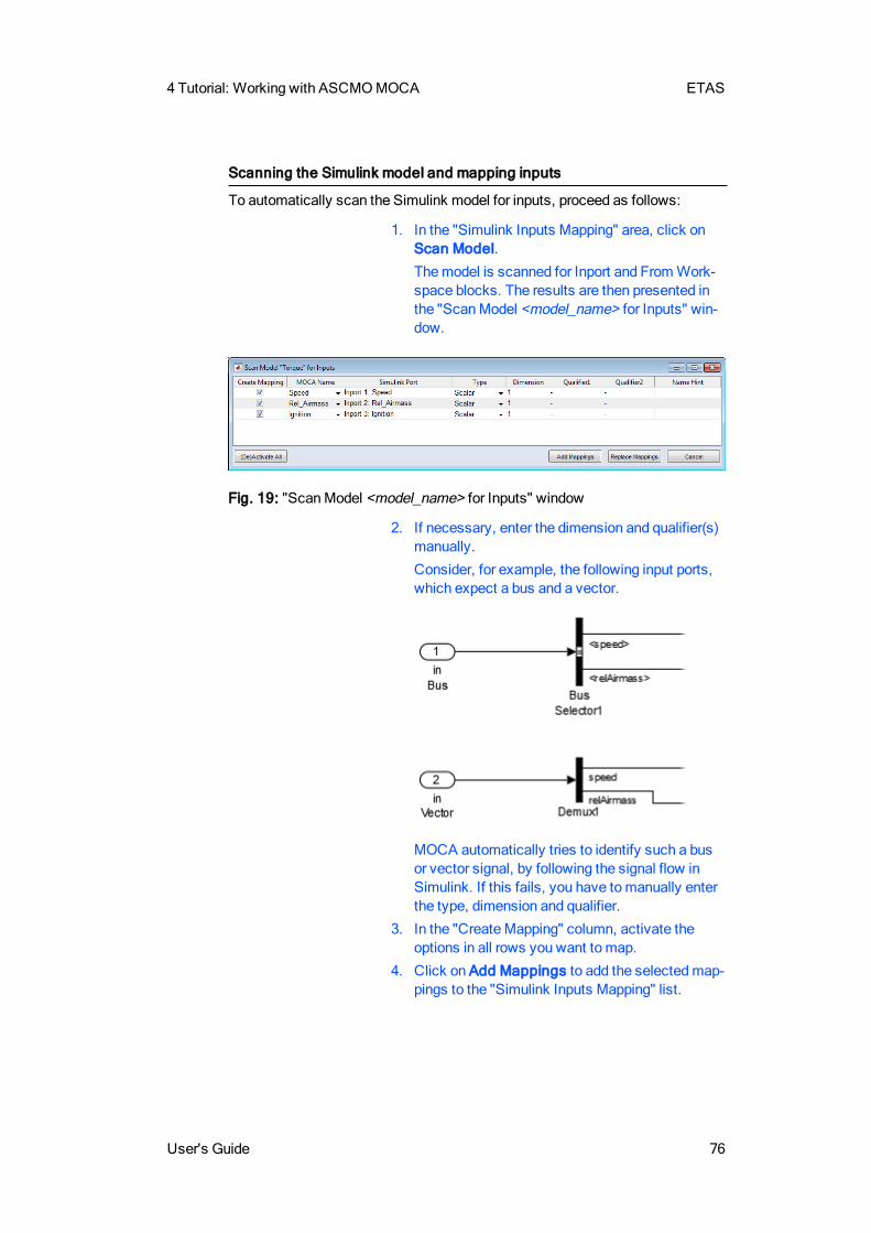
4 Tutorial: Working with ASCMOMOCA ETAS
User's Guide 76
Scanning the Simulink model and mapping inputs
To automatically scan the Simulink model for inputs, proceed as follows:
1. In the "Simulink Inputs Mapping" area, click onScan Model.
Themodel is scanned for Inport and FromWork-space blocks. The results are then presented inthe "ScanModel <model_name> for Inputs" win-dow.
Fig. 19: "ScanModel <model_name> for Inputs" window
2. If necessary, enter the dimension and qualifier(s)manually.
Consider, for example, the following input ports,which expect a bus and a vector.
MOCA automatically tries to identify such a busor vector signal, by following the signal flow inSimulink. If this fails, you have tomanually enterthe type, dimension and qualifier.
3. In the "CreateMapping" column, activate theoptions in all rows you want to map.
4. Click on Add Mappings to add the selectedmap-pings to the "Simulink Inputs Mapping" list.
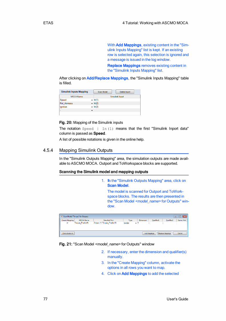
ETAS 4 Tutorial: Working with ASCMOMOCA
77 User's Guide
With Add Mappings, existing content in the "Sim-ulink Inputs Mapping" list is kept. If an existingrow is selected again, this selection is ignored andamessage is issued in the log window.
Replace Mappings removes existing content inthe "Simulink Inputs Mapping" list.
After clicking on Add/Replace Mappings, the "Simulink Inputs Mapping" tableis filled.
Fig. 20: Mapping of the Simulink inputs
The notation Speed | In(1) means that the first "Simulink Inport data"column is passed as Speed.
A list of possible notations is given in the online help.
4.5.4 Mapping Simulink Outputs
In the "Simulink Outputs Mapping" area, the simulation outputs are made avail-able to ASCMOMOCA. Outport and ToWorkspace blocks are supported.
Scanning the Simulink model and mapping outputs
1. 1. In the "Simulink Outputs Mapping" area, click onScan Model.
Themodel is scanned for Outport and ToWork-space blocks. The results are then presented inthe "ScanModel <model_name> for Outputs" win-dow.
Fig. 21: "ScanModel <model_name> for Outputs" window
2. If necessary, enter the dimension and qualifier(s)manually.
3. In the "CreateMapping" column, activate theoptions in all rows you want to map.
4. Click on Add Mappings to add the selected
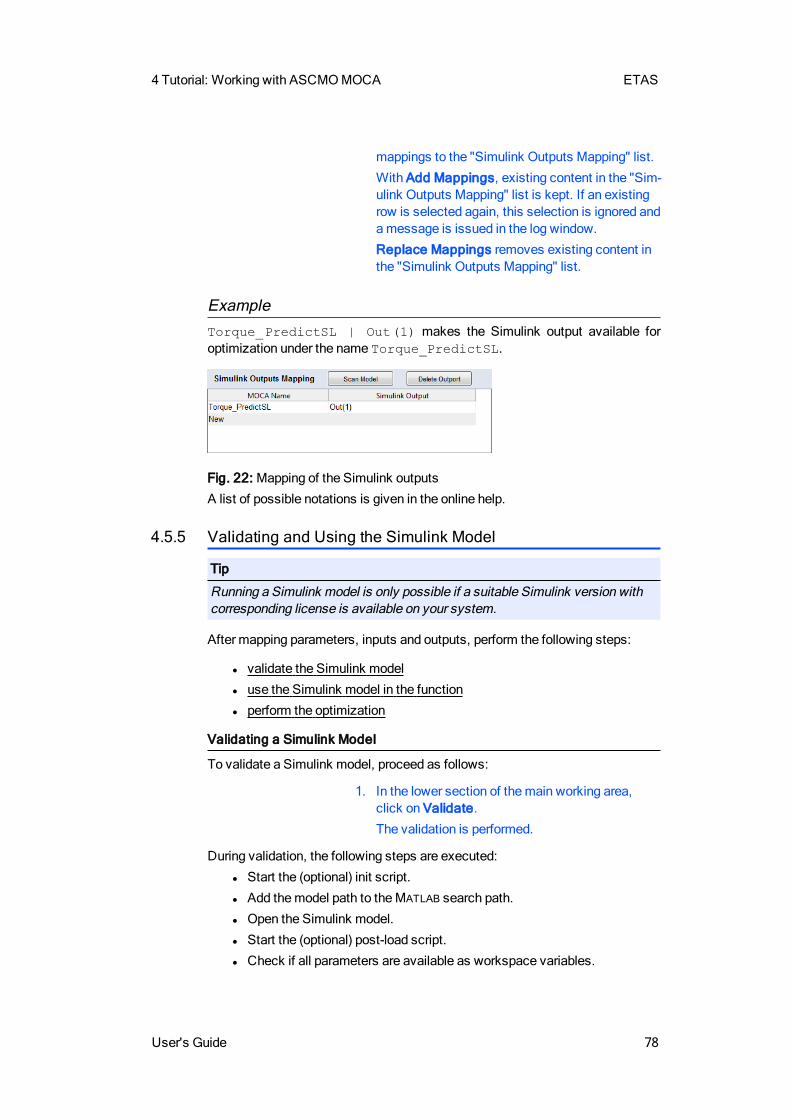
4 Tutorial: Working with ASCMOMOCA ETAS
User's Guide 78
mappings to the "Simulink Outputs Mapping" list.
With Add Mappings, existing content in the "Sim-ulink Outputs Mapping" list is kept. If an existingrow is selected again, this selection is ignored andamessage is issued in the log window.
Replace Mappings removes existing content inthe "Simulink Outputs Mapping" list.
ExampleTorque_PredictSL | Out(1) makes the Simulink output available foroptimization under the name Torque_PredictSL.
Fig. 22: Mapping of the Simulink outputs
A list of possible notations is given in the online help.
4.5.5 Validating and Using the Simulink Model
Tip
Running a Simulink model is only possible if a suitable Simulink version withcorresponding license is available on your system.
After mapping parameters, inputs and outputs, perform the following steps:
l validate the Simulink model
l use the Simulink model in the function
l perform the optimization
Validating a Simulink Model
To validate a Simulink model, proceed as follows:
1. In the lower section of themain working area,click on Validate.
The validation is performed.
During validation, the following steps are executed:
l Start the (optional) init script.
l Add themodel path to theMATLAB search path.
l Open the Simulink model.
l Start the (optional) post-load script.
l Check if all parameters are available as workspace variables.
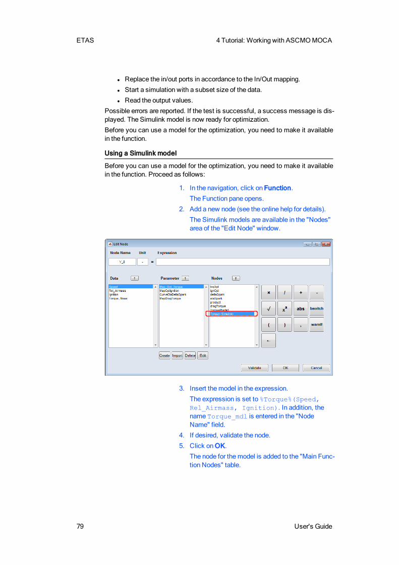
ETAS 4 Tutorial: Working with ASCMOMOCA
79 User's Guide
l Replace the in/out ports in accordance to the In/Out mapping.
l Start a simulation with a subset size of the data.
l Read the output values.
Possible errors are reported. If the test is successful, a success message is dis-played. The Simulink model is now ready for optimization.
Before you can use a model for the optimization, you need to make it availablein the function.
Using a Simulink model
Before you can use a model for the optimization, you need to make it availablein the function. Proceed as follows:
1. In the navigation, click on Function.
The Function pane opens.
2. Add a new node (see the online help for details).
The Simulink models are available in the "Nodes"area of the "Edit Node" window.
3. Insert themodel in the expression.
The expression is set to %Torque%(Speed,Rel_Airmass, Ignition). In addition, thename Torque_mdl is entered in the "NodeName" field.
4. If desired, validate the node.
5. Click onOK.
The node for themodel is added to the "Main Func-tion Nodes" table.
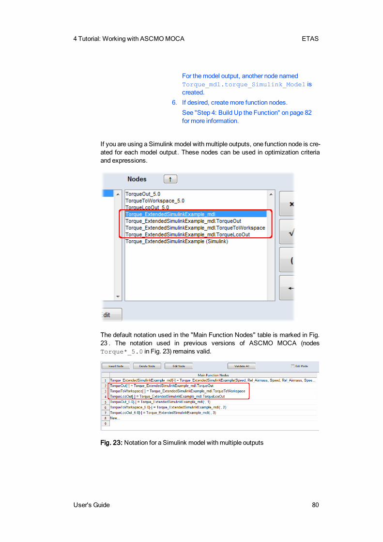
4 Tutorial: Working with ASCMOMOCA ETAS
User's Guide 80
For themodel output, another node namedTorque_mdl.torque_Simulink_Model iscreated.
6. If desired, createmore function nodes.
See "Step 4: Build Up the Function" on page 82for more information.
If you are using a Simulink model with multiple outputs, one function node is cre-ated for each model output. These nodes can be used in optimization criteriaand expressions.
The default notation used in the "Main Function Nodes" table is marked in Fig.23 . The notation used in previous versions of ASCMO MOCA (nodesTorque*_5.0 in Fig. 23) remains valid.
Fig. 23: Notation for a Simulink model with multiple outputs
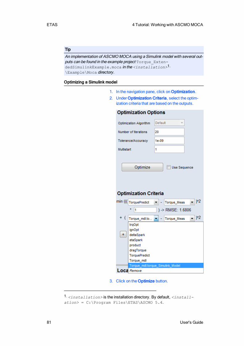
ETAS 4 Tutorial: Working with ASCMOMOCA
81 User's Guide
Tip
An implementation of ASCMOMOCA using a Simulink model with several out-puts can be found in the example project Torque_Exten-dedSimulinkExample.moca in the <installation>1.\Example\Moca directory.
Optimizing a Simulink model
1. In the navigation pane, click onOptimization.
2. Under Optimization Criteria, select the optim-ization criteria that are based on the outputs.
3. Click on the Optimize button.
1. <installation> is the installation directory. By default, <install-ation> = C:\Program Files\ETAS\ASCMO 5.4.
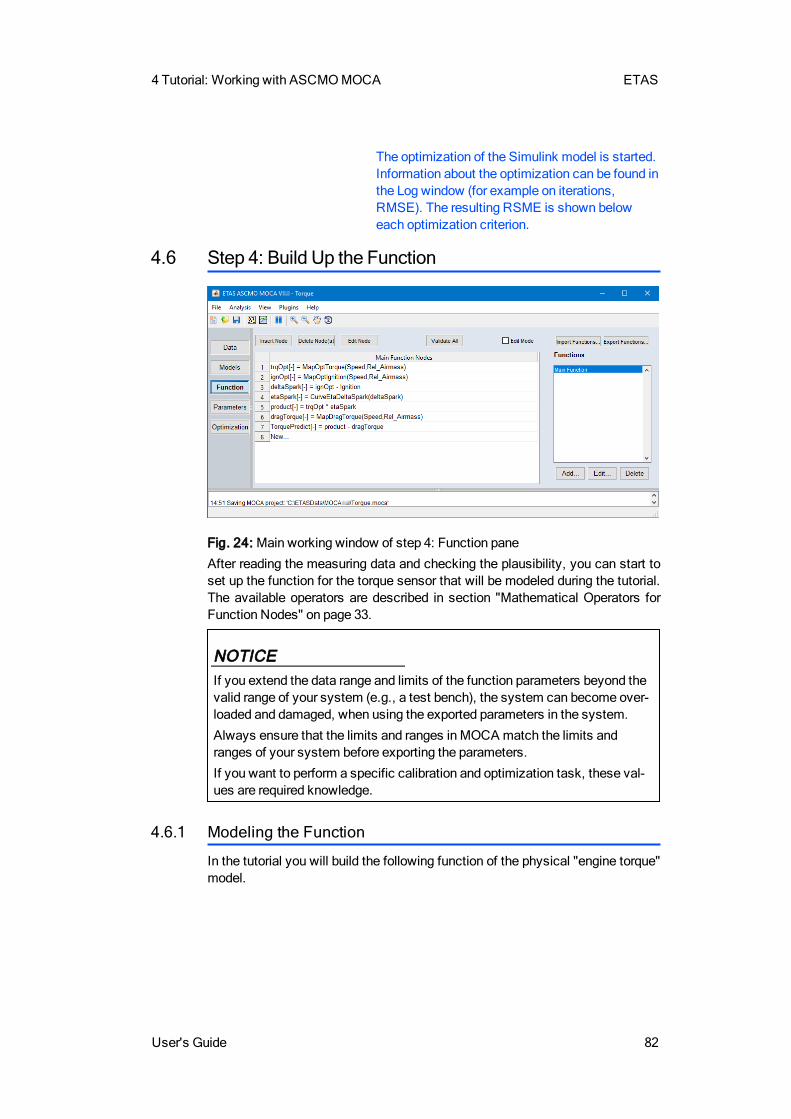
4 Tutorial: Working with ASCMOMOCA ETAS
User's Guide 82
The optimization of the Simulink model is started.Information about the optimization can be found inthe Log window (for example on iterations,RMSE). The resulting RSME is shown beloweach optimization criterion.
4.6 Step 4: Build Up the Function
Fig. 24: Main working window of step 4: Function pane
After reading the measuring data and checking the plausibility, you can start toset up the function for the torque sensor that will be modeled during the tutorial.The available operators are described in section "Mathematical Operators forFunction Nodes" on page 33.
NOTICEIf you extend the data range and limits of the function parameters beyond thevalid range of your system (e.g., a test bench), the system can become over-loaded and damaged, when using the exported parameters in the system.
Always ensure that the limits and ranges inMOCA match the limits andranges of your system before exporting the parameters.
If you want to perform a specific calibration and optimization task, these val-ues are required knowledge.
4.6.1 Modeling the Function
In the tutorial you will build the following function of the physical "engine torque"model.
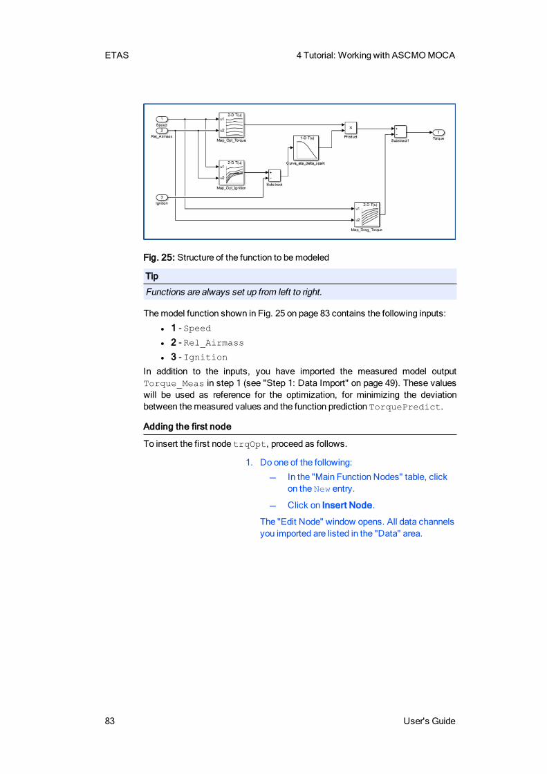
ETAS 4 Tutorial: Working with ASCMOMOCA
83 User's Guide
Fig. 25: Structure of the function to bemodeled
Tip
Functions are always set up from left to right.
Themodel function shown in Fig. 25 on page 83 contains the following inputs:
l 1 - Speed
l 2 - Rel_Airmass
l 3 - Ignition
In addition to the inputs, you have imported the measured model outputTorque_Meas in step 1 (see "Step 1: Data Import" on page 49). These valueswill be used as reference for the optimization, for minimizing the deviationbetween themeasured values and the function prediction TorquePredict.
Adding the first node
To insert the first node trqOpt, proceed as follows.
1. Do one of the following:
In the "Main Function Nodes" table, clickon the New entry.
Click on Insert Node.
The "Edit Node" window opens. All data channelsyou imported are listed in the "Data" area.
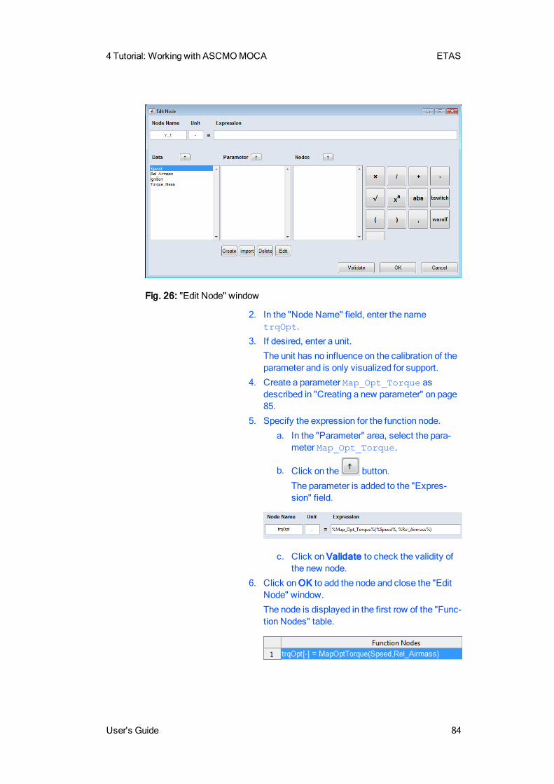
4 Tutorial: Working with ASCMOMOCA ETAS
User's Guide 84
Fig. 26: "Edit Node" window
2. In the "Node Name" field, enter the nametrqOpt.
3. If desired, enter a unit.
The unit has no influence on the calibration of theparameter and is only visualized for support.
4. Create a parameter Map_Opt_Torque asdescribed in "Creating a new parameter" on page85.
5. Specify the expression for the function node.
a. In the "Parameter" area, select the para-meter Map_Opt_Torque.
b. Click on the button.
The parameter is added to the "Expres-sion" field.
c. Click on Validate to check the validity ofthe new node.
6. Click onOK to add the node and close the "EditNode" window.
The node is displayed in the first row of the "Func-tion Nodes" table.
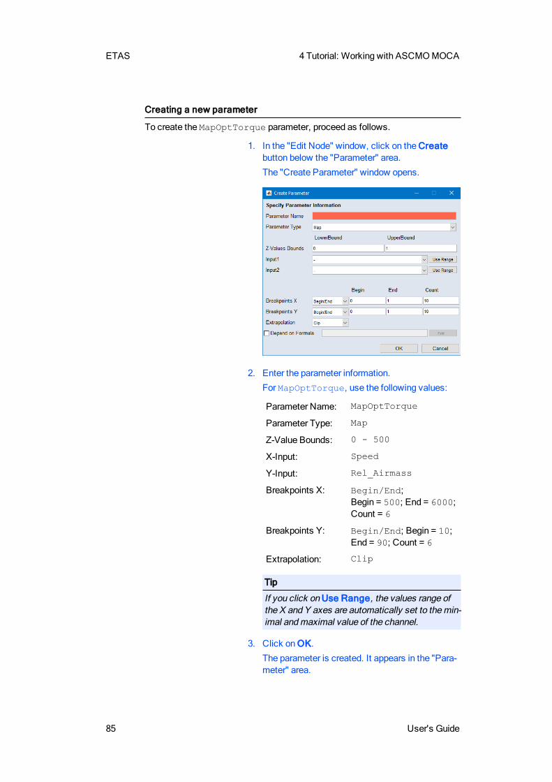
ETAS 4 Tutorial: Working with ASCMOMOCA
85 User's Guide
Creating a new parameter
To create the MapOptTorque parameter, proceed as follows.
1. In the "Edit Node" window, click on the Createbutton below the "Parameter" area.
The "Create Parameter" window opens.
2. Enter the parameter information.
For MapOptTorque, use the following values:
Parameter Name: MapOptTorque
Parameter Type: Map
Z-Value Bounds: 0 - 500
X-Input: Speed
Y-Input: Rel_Airmass
Breakpoints X: Begin/End;Begin = 500; End = 6000;Count = 6
Breakpoints Y: Begin/End; Begin = 10;End = 90; Count = 6
Extrapolation: Clip
Tip
If you click on Use Range, the values range ofthe X and Y axes are automatically set to themin-imal andmaximal value of the channel.
3. Click onOK.
The parameter is created. It appears in the "Para-meter" area.
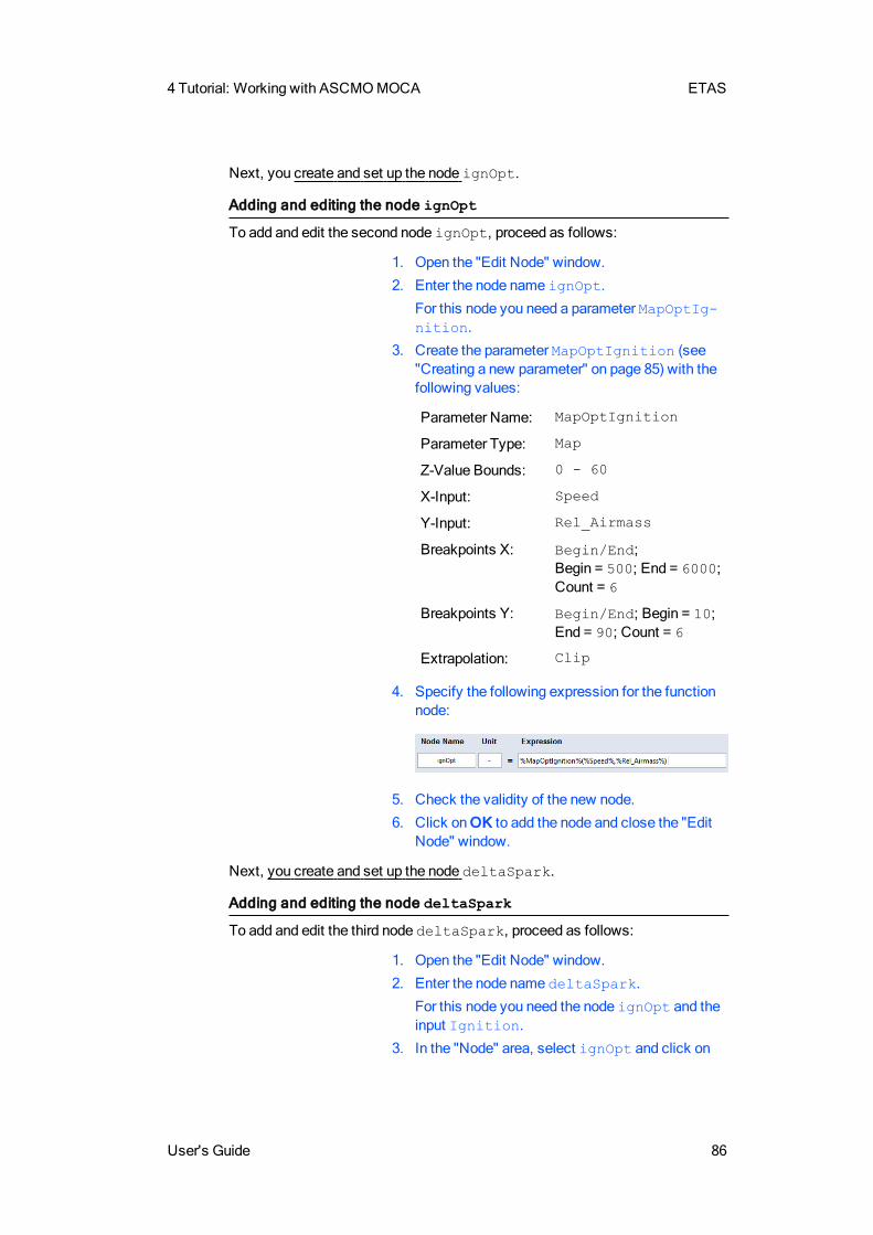
4 Tutorial: Working with ASCMOMOCA ETAS
User's Guide 86
Next, you create and set up the node ignOpt.
Adding and editing the node ignOpt
To add and edit the second node ignOpt, proceed as follows:
1. Open the "Edit Node" window.
2. Enter the node name ignOpt.
For this node you need a parameter MapOptIg-nition.
3. Create the parameter MapOptIgnition (see"Creating a new parameter" on page 85) with thefollowing values:
Parameter Name: MapOptIgnition
Parameter Type: Map
Z-Value Bounds: 0 - 60
X-Input: Speed
Y-Input: Rel_Airmass
Breakpoints X: Begin/End;Begin = 500; End = 6000;Count = 6
Breakpoints Y: Begin/End; Begin = 10;End = 90; Count = 6
Extrapolation: Clip
4. Specify the following expression for the functionnode:
5. Check the validity of the new node.
6. Click onOK to add the node and close the "EditNode" window.
Next, you create and set up the node deltaSpark.
Adding and editing the node deltaSpark
To add and edit the third node deltaSpark, proceed as follows:
1. Open the "Edit Node" window.
2. Enter the node name deltaSpark.
For this node you need the node ignOpt and theinput Ignition.
3. In the "Node" area, select ignOpt and click on
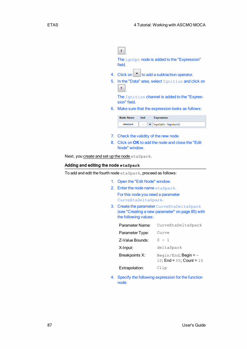
ETAS 4 Tutorial: Working with ASCMOMOCA
87 User's Guide
.
The ignOpt node is added to the "Expression"field.
4. Click on to add a subtraction operator.
5. In the "Data" area, select Ignition and click on
.
The Ignition channel is added to the "Expres-sion" field.
6. Make sure that the expression looks as follows:
7. Check the validity of the new node.
8. Click onOK to add the node and close the "EditNode" window.
Next, you create and set up the node etaSpark.
Adding and editing the node etaSpark
To add and edit the fourth node etaSpark, proceed as follows:
1. Open the "Edit Node" window.
2. Enter the node name etaSpark.
For this node you need a parameterCurveEtaDeltaSpark.
3. Create the parameter CurveEtaDeltaSpark(see "Creating a new parameter" on page 85) withthe following values:
Parameter Name: CurveEtaDeltaSpark
Parameter Type: Curve
Z-Value Bounds: 0 - 1
X-Input: deltaSpark
Breakpoints X: Begin/End; Begin = -10; End = 55; Count = 10
Extrapolation: Clip
4. Specify the following expression for the functionnode:
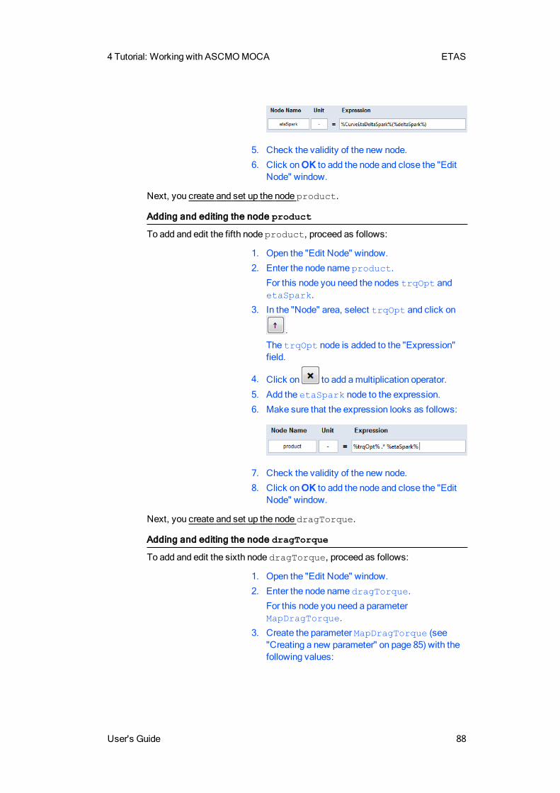
4 Tutorial: Working with ASCMOMOCA ETAS
User's Guide 88
5. Check the validity of the new node.
6. Click onOK to add the node and close the "EditNode" window.
Next, you create and set up the node product.
Adding and editing the node product
To add and edit the fifth node product, proceed as follows:
1. Open the "Edit Node" window.
2. Enter the node name product.
For this node you need the nodes trqOpt andetaSpark.
3. In the "Node" area, select trqOpt and click on
.
The trqOpt node is added to the "Expression"field.
4. Click on to add amultiplication operator.
5. Add the etaSpark node to the expression.
6. Make sure that the expression looks as follows:
7. Check the validity of the new node.
8. Click onOK to add the node and close the "EditNode" window.
Next, you create and set up the node dragTorque.
Adding and editing the node dragTorque
To add and edit the sixth node dragTorque, proceed as follows:
1. Open the "Edit Node" window.
2. Enter the node name dragTorque.
For this node you need a parameterMapDragTorque.
3. Create the parameter MapDragTorque (see"Creating a new parameter" on page 85) with thefollowing values:
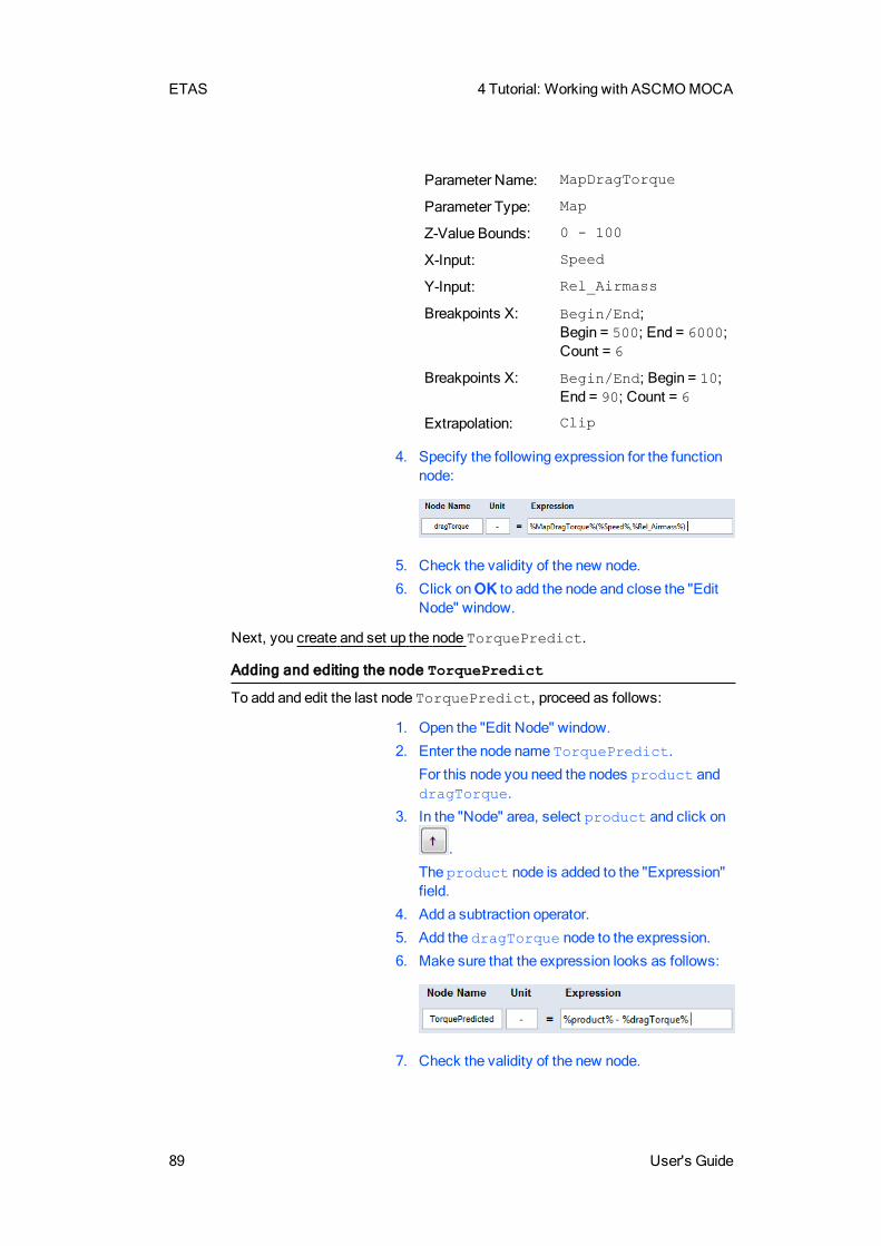
ETAS 4 Tutorial: Working with ASCMOMOCA
89 User's Guide
Parameter Name: MapDragTorque
Parameter Type: Map
Z-Value Bounds: 0 - 100
X-Input: Speed
Y-Input: Rel_Airmass
Breakpoints X: Begin/End;Begin = 500; End = 6000;Count = 6
Breakpoints X: Begin/End; Begin = 10;End = 90; Count = 6
Extrapolation: Clip
4. Specify the following expression for the functionnode:
5. Check the validity of the new node.
6. Click onOK to add the node and close the "EditNode" window.
Next, you create and set up the node TorquePredict.
Adding and editing the node TorquePredict
To add and edit the last node TorquePredict, proceed as follows:
1. Open the "Edit Node" window.
2. Enter the node name TorquePredict.
For this node you need the nodes product anddragTorque.
3. In the "Node" area, select product and click on
.
The product node is added to the "Expression"field.
4. Add a subtraction operator.
5. Add the dragTorque node to the expression.
6. Make sure that the expression looks as follows:
7. Check the validity of the new node.
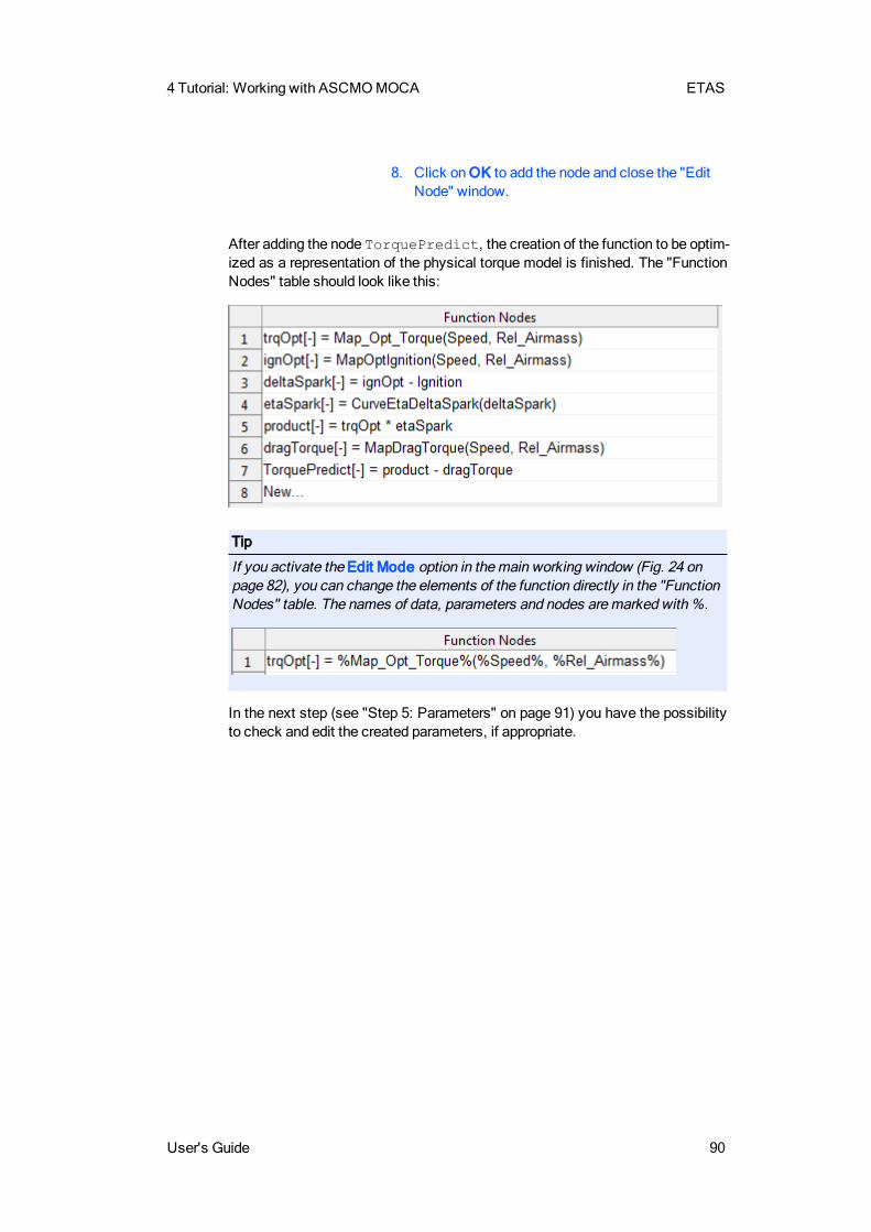
4 Tutorial: Working with ASCMOMOCA ETAS
User's Guide 90
8. Click onOK to add the node and close the "EditNode" window.
After adding the node TorquePredict, the creation of the function to be optim-ized as a representation of the physical torque model is finished. The "FunctionNodes" table should look like this:
Tip
If you activate the Edit Mode option in themain working window (Fig. 24 onpage 82), you can change the elements of the function directly in the "FunctionNodes" table. The names of data, parameters and nodes aremarked with%.
In the next step (see "Step 5: Parameters" on page 91) you have the possibilityto check and edit the created parameters, if appropriate.
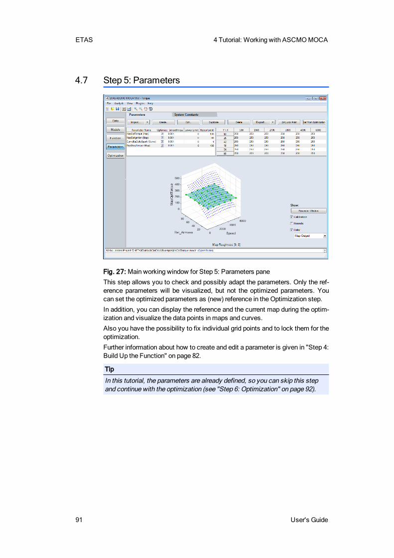
ETAS 4 Tutorial: Working with ASCMOMOCA
91 User's Guide
4.7 Step 5: Parameters
Fig. 27: Main working window for Step 5: Parameters pane
This step allows you to check and possibly adapt the parameters. Only the ref-erence parameters will be visualized, but not the optimized parameters. Youcan set the optimized parameters as (new) reference in the Optimization step.
In addition, you can display the reference and the current map during the optim-ization and visualize the data points in maps and curves.
Also you have the possibility to fix individual grid points and to lock them for theoptimization.
Further information about how to create and edit a parameter is given in "Step 4:Build Up the Function" on page 82.
Tip
In this tutorial, the parameters are already defined, so you can skip this stepand continue with the optimization (see "Step 6: Optimization" on page 92).
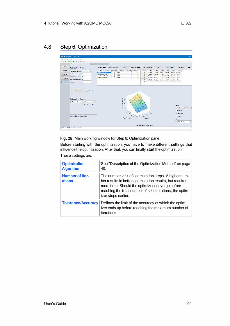
4 Tutorial: Working with ASCMOMOCA ETAS
User's Guide 92
4.8 Step 6: Optimization
Fig. 28: Main working window for Step 6: Optimization pane
Before starting with the optimization, you have to make different settings thatinfluence the optimization. After that, you can finally start the optimization.
These settings are:
OptimizationAlgorithm
See "Description of the OptimizationMethod" on page40.
Number of Iter-ations
The number <i> of optimization steps. A higher num-ber results in better optimization results, but requiresmore time. Should the optimizer converge beforereaching the total number of <i> iterations, the optim-izer stops earlier.
Tolerance/Accuracy Defines the limit of the accuracy at which the optim-izer ends up before reaching themaximum number ofiterations.
ETAS 4 Tutorial: Working with ASCMOMOCA
93 User's Guide
Finite DifferenceFactor
When using external models, gradients are calculatedusing finite differences with the following formula:
gradient = (f(x+e)−f(x))/e
with e = FiniteDifferenceFactor*10^-16
One is default, only change this, if the optimizer stopsdirectly after the first iteration. This might happen,when themodel isn't sensitive to (normalized) para-meter change of 10^-16.
Multistart Defines the number <n> of optimization runs. A highernumber results in better optimization results, butrequires more time. Should the optimizer convergebefore the end of the <n>th optimization run, the optim-izer stops earlier.
If, e.g., you set the number of iterations to 10 and theMultistart value to 5, the total max. number of iter-ations is 50.
Tip
The above listed criteria and limits have to be adapted for the specific problem,such that a satisfactory minimal deviation ( see "Variables RMSE and R2" onpage 29) between themeasured data and the function prediction can bereached by optimization.
Preparing the optimization
In the "Optimization Options" area, you specify several parameters; see "Optim-ization Options" on page 1.
In the "Optimization Criteria" area, you specify the optimization target. Youselect a function node in the first combo box and a data channel (or '0') in thesecond combo box. The optimizer will then try to find a set of parameter valuesthat minimizes the quadratic deviation of those two quantities.
The "Local Hard Constraints" area is not used in this tutorial.
1. In the "Optimization Options" area, do the fol-lowing:
a. In the "Number of Iterations" field (cf. Fig.28 on page 92), enter a number of 40 iter-ations.
b. If desired, increase the number in the"Multistart" field.
2. In the "Optimization Criteria" area, do the fol-lowing:

4 Tutorial: Working with ASCMOMOCA ETAS
User's Guide 94
a. In the first combo box, select the functionoutput TorquePredict.
b. In the second combo box, select the impor-ted data channel Torque_Meas.
The flat parameters results in a high RMSE(see "Variables RMSE and R2" on page29). After the first optimization, the RMSEwill be significantly reduced.
Note that you have the possibility to define a sum
of such optimization criteria using the Add anew Optimization criterium button.
Performing the optimization
Once you have finished the preparations, start the optimization.
1. Click onOptimize.
The optimizer starts with the optimization of theparameters. Information about the optimizationcan be found in the Log window (for example oniterations, RMSE). The resulting RSME is shownbelow the optimization criterion. The visualization
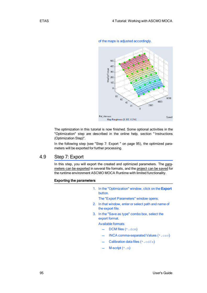
ETAS 4 Tutorial: Working with ASCMOMOCA
95 User's Guide
of themaps is adjusted accordingly.
The optimization in this tutorial is now finished. Some optional activities in the"Optimization" step are described in the online help, section " Instructions(Optimization Step)".
In the following step (see "Step 7: Export " on page 95), the optimized para-meters will be exported for further processing.
4.9 Step 7: ExportIn this step, you will export the created and optimized parameters. The para-meters can be exported in several file formats, and the project can be saved forthe runtime environment ASCMOMOCA Runtime with limited functionality.
Exporting the parameters
1. In the "Optimization" window, click on the Exportbutton.
The "Export Parameters" window opens.
2. In that window, enter or select path and name ofthe export file.
3. In the "Save as type" combo box, select theexport format.
Available formatsDCM files (*.dcm)
INCA comma-separated Values (*.csv)
Calibration data files (*.cdfx)
M-script (*.m)
4 Tutorial: Working with ASCMOMOCA ETAS
User's Guide 96
4. Click on Save.
The parameters will be exported to a file in theselected format.
Exporting the project for ASCMO MOCA Runtime
When you export a project to ASCMOMOCA Runtime, the project gets encryp-ted, and the function in the project cannot be seen or edited.
1. In themainmenu, select File → Export toMOCA-Runtime.
The "Export to MOCA-Runtime" window opens.
2. Activate Show Sequence if you want to showthe optimization sequence in the exported pro-ject.
With that, you can see and edit the sequence inASCMOMOCA Runtime. The sequence is hid-den if Show Sequence remains deactivated.
3. Activate Allow opening in Matlab (MOCA-Runtime p-Code) to allow the exported project tobe opened in the p-Code version of ASCMOMOCA Runtime.
If you activate Allow opening in Matlab (MOCARuntime p-Code), the exported project getsencrypted with another key. ASCMOMOCARuntime p-Code cannot open exported projectswithout this setting. Such projects can only beopened with the standalone version of ASCMOMOCA Runtime.
4. Click on Export to continue.
The "Export MOCA project to MOCA-Runtime"window opens. The *.moca_runtime format ispreselected; it is mandatory.
5. Enter the file name and the file directory.
6. Click on Save.
The project is saved for ASCMOMOCA Runtime.
ETAS 5 ETAS Contact Addresses
97 User's Guide
5 ETAS Contact Addresses
ETAS Headquarter
ETAS GmbH
Borsigstraße 24 Phone: +49 711 3423-0
70469 Stuttgart FAX: +49 711 3423-2106
Germany Internet: www.etas.com
ETAS Subsidiaries and Technical Support
For details of your local sales office as well as your local technical support teamand product hotlines, take a look at the ETAS website:
ETAS subsidiaries Internet: www.etas.com/en/contact.php
ETAS technical sup-port:
Internet: www.etas.com/en/hotlines.php
FiguresFig. 1: Themain user interface elements of ASCMOMOCA 20
Fig. 2: Information in the log window (example; a: link to the online help, b: link to thePDFmanual) 23
Fig. 3: The "All Data" window 24
Fig. 4: The "Data and Nodes" window 26
Fig. 5: The "Histogram" window 27
Fig. 6: The "Residuals over Inputs" window 28
Fig. 7: The "Measured vs. Predicted" window 29
Fig. 8: "Create Parameter" or "Edit Parameter" window for scalar, curve, map, Cube-3D and Cube-4D parameters (a: available for curve, map, Cube-3D and Cube-4D para-meters, b: available for map, Cube-3D and Cube-4D parameters, c: available for Cube-3D and Cube-4D parameters, d: available for Cube-4D parameters) 36
Fig. 9: "Parameter optimization properties" window 42
Fig. 10: Normalized parameter sensitivity 44
Fig. 11: ETAS ASCMOMOCA start window 48
Fig. 12: View after the start of ASCMOMOCA 49
Fig. 13: Main working window for Step 1: Data pane 49
Fig. 14: "MOCA Data Import" window 51
Fig. 15: Main working window for Step 3: Models pane 71
Fig. 16: Main working area with additional options 72
Fig. 17: Table data and breakpoints from Simulink map 73
Fig. 18: "ScanModel <model_name> for Parameter Mapping" window 74
Fig. 19: "ScanModel <model_name> for Inputs" window 76
Figures ETAS
User's Guide 98
Fig. 20: Mapping of the Simulink inputs 77
Fig. 21: "ScanModel <model_name> for Outputs" window 77
Fig. 22: Mapping of the Simulink outputs 78
Fig. 23: Notation for a Simulink model with multiple outputs 80
Fig. 24: Main working window of step 4: Function pane 82
Fig. 25: Structure of the function to bemodeled 83
Fig. 26: "Edit Node" window 84
Fig. 27: Main working window for Step 5: Parameters pane 91
Fig. 28: Main working window for Step 6: Optimization pane 92
ETAS Glossary
99 User's Guide
FormulasEqu. 1: Root Mean Squared Error (RMSE) 29
Equ. 2: Sum of Squared Residuals (SSR) 30
Equ. 3: Coefficient of determination R2 30
Equ. 4: Total Sum of Squares (SST) 30
Equ. 5: Optimizationmethod 40
Equ. 6: Roughness r of a curve 40
Equ. 7: Roughness of amap 41
Equ. 8: Smoothness factor Si 41
Formulas ETAS
User's Guide 100
Index ETAS
User's Guide 101
IndexA
ASCMOmodel 32
C
CharacteristicRMSE 29
Compressedmodel 38Concept 17
assessment of input data 23parameter optimization 35
Configuration fileload 55save 55
contacts 97Correlation
of parameters 43
D
Datacheck plausibility 51check relevance 24, 54filter 63remove NaN 63sort 64
Data analysis 65Data point
activate/deactivate 60delete 65
edit 62set weight 61weight 61
Data qualityassessment 25improvement 25
Data set See also Measurement datadelete 60loadmultiple 58multiple 58rename 59weight 61
E
Error Analysisabsolute 26data 25function node 25relative 26Residual Analysis 26studentized 26
ETAScontacts 97
F
Fields of application 17ASCMOMOCA 18ASCMOMOCA Runtime 18
Filter data 63FMU model 31Formulas 100Function
add node 83create 82mathematical operators 33structure 82
Function evaluationR^2 30RMSE 31
Function variablechange name 57deletemapping 57mapmeasurement channel 57
I
Import 49display data 51load configuration 55measurement data 49save configuration 55start 56
Input dataassessment 23improvement 23
Inputsrelevance 24, 54
Installation 10directories 15files 15license agreement 11path specification 12preparation 10start 11system requirements 10uninstall MOCA 16user privileges 10
L
Licensing 15Log file
save 23
M
Matlab/Simulinkselect version 71
Measurement data See also Data setdelete channel 65deletemapping to variable 57
import 56map channel to variable 57plausibility check 51requirements 47
Measurement fileformat 47load 50
Methods 17MOCA
start 48start from within Matlab 44uninstall 16
MOCA RuntimeExport to 96Export to p-Code version 96start from within Matlab 44
Models 31add Simulink model 71ASCET 31ASCMODynamic 32ASCMOStatic 32FMU 31map parameters 73map Simulink inputs 75map Simulink outputs 77Simulink 71
N
Nodesadd 83Mathematical operators 33
O
Optimization 39, 42, 92Parameter 35Simulink model 81with sequence 42
Optimization criterion 41Optimizationmethod
Description 40Outlier
delete 68
P
p-Code version 44, 96Parameter optimization 35Parameters 35
3D cube 384D cube 38check 91
ETAS Index
102 User's Guide
compressedmodel 38correlation 43create 85curve 37edit 91export 95lookup-table 37map 37map to Simulink
parameters 73matrix 39scalar 38sensitivity 43types 35
Plausibility check 51
Q
QualityEvaluation 30
R
R^2 29-30RMSE 29Root Mean Square Error 29Roughness 40
of a curve 40of amap 40
S
Safety Information 6Scatter plot
select axes 66Sensitivity
of parameters 43Sequence
for optimization 42, 96inMOCA Runtime 96
Simulink model 71add 71optimize 81
Sort data 64Start MOCA 48System constant 39
T
Toolbar 20Tutorial 46
create function 82data analysis 65
data import 49measurement data 47models 71
U
User interfaceLog window 23main elements 20navigation pane 21toolbar 20
V
Variable See Function variable
W
Weightdata point 61data set 61
Working stepscreate function 82data analysis 65data import 49Exporting parameters 95models 71Parameter optimization 92
Index ETAS
User's Guide 103