Eta-Invariants and Molien Series for Unimodular Groups

by

Anda Degeratu

B.A., University of Bucharest, 1996

Submitted to the Department of Mathematicsin partial fulfillment of the requirements for the degree of

Doctor of Philosophy

at the

MASSACHUSETTS INSTITUTE OF TECHNOLOGY

September 2001

c© Anda Degeratu, MMI. All rights reserved.

The author hereby grants to MIT permission to reproduce and distribute publiclypaper and electronic copies of this thesis document in whole or in part and to grant

others the right to do so.

Author . . . . . . . . . . . . . . . . . . . . . . . . . . . . . . . . . . . . . . . . . . . . . . . . . . . . . . . . . . . . . . . . . . . . . . . . . . . .Department of Mathematics

September 3, 2001

Certified by. . . . . . . . . . . . . . . . . . . . . . . . . . . . . . . . . . . . . . . . . . . . . . . . . . . . . . . . . . . . . . . . . . . . . . . .Tomasz S. Mrowka

Professor of MathematicsThesis Supervisor

Accepted by . . . . . . . . . . . . . . . . . . . . . . . . . . . . . . . . . . . . . . . . . . . . . . . . . . . . . . . . . . . . . . . . . . . . . . .Tomasz S. Mrowka

Chairman, Department Committee on Graduate Students

2

Eta-Invariants and Molien Series for Unimodular Groupsby

Anda Degeratu

Submitted to the Department of Mathematicson September 3, 2001, in partial fulfillment of the

requirements for the degree ofDoctor of Philosophy

Abstract

We look at the singularity Cn/Γ, for Γ finite subgroup of SU(n), from two perspectives.From a geometrical point of view, Cn/Γ is an orbifold with boundary S2n−1/Γ. We defineand compute the corresponding orbifold η-invariant. From an algebraic point of view, welook at the algebraic variety Cn/Γ and we analyze the associated Molien series. The mainresult is a formula which relates the two notions: η-invariant and Molien series. Along theway computations of the spectrum of the Dirac operator on the sphere are performed.

Thesis Supervisor: Tomasz S. MrowkaTitle: Professor of Mathematics

3

4

Acknowledgments

First of all I want to thank my advisor, Tom Mrowka, for everything he taught me. Fromhim I learned what it means to do research, how to ask myself questions and how to proceedtowards finding an answer to them. It was always extremely enlightening to talk to himand see his way of thinking. He’s also been a great friend and a source of tremendous moralsupport during my life in graduate school.

The direction of my research was influenced by a wonderful class taught by Peter Kron-heimer in my first semester in graduate school. I thank Peter for this and for the instructiveconversations we had this last year.

During my life in graduate school I had two mentors: Elly Ionel and Allen Knutson.Patiently they both answered to all my naive questions which I was asking over and overagain. I thank Allen for teaching me representation theory and for suggesting the Gelfand-Cetlin method to solve the spectrum problem.

To Carmen Young, my dear friend, my officemate and my academic sister, I am gratefulfor the uncountable times she said to me: “Just do it!” Warmest thanks to Ana-MariaCastravet. She shared with me her intransigent points of view; but, then she was alwaysready to give me a chance, and this led to passionate discussions and extremely interestingdiscoveries for both of us. Gudarz Davar was willing to dive along with me into the intricatequestions about life and research. Thanks, Gudarz! Jianmei Wang and I had an extremelyintense summer. I was writing this thesis and in the same time we were doing such anamazing amount of cool things; it helped me so much!

I thank Benoit Charboneaux and Michael Gruber for being such great friends. To myacademic siblings Lenny Ng, Carmen Young, Yue Lei, Edward Goldstein, Aleksey Zinger Iam extremely thankful for all the talks they gave in Tom’s students seminar. I thank Tomand Lenny for generously moving the content of their bookshelves on mine! I enjoyed a lotthe company of the people who used to inhabit the office 2-229: Dana Pascovici, GustavoGranja, Sergiu Moroianu, Phil Bradley, Collin Ingalls, Ioanid Rosu, Richard Stone. I thankall of them for the joy with which they either talked about math or invented new rules forthe world.

I am extremely grateful to Linda Okun for all the nice words and sweet candies she hadfor me. And I thank Jessica Barton for helping me understand who I am and what I want.

My warmest thoughts go to my parents and my sister, Melania. During all these yearsmy parents always put us first and made sure that we always get the best that exists. Theycontinuously supported me, even from far away, in the difficult years in graduate school.Their love and faith in me is a permanent source of energy.

5

6

Contents

1 Introduction 9

2 Homogeneous Spaces 132.1 Crash course in Representation Theory . . . . . . . . . . . . . . . . . . . . . 132.2 Homogeneous Spaces and Homogeneous Structures on Them . . . . . . . . 17

2.2.1 Homogeneous Riemannian structures . . . . . . . . . . . . . . . . . . 172.2.2 Riemannian connections on homogeneous spaces . . . . . . . . . . . 182.2.3 Homogeneous vector bundles . . . . . . . . . . . . . . . . . . . . . . 202.2.4 Homogeneous Differential operators . . . . . . . . . . . . . . . . . . 21

2.3 Spin structures and Dirac operators on Homogeneous manifolds . . . . . . 212.3.1 The Dirac operator . . . . . . . . . . . . . . . . . . . . . . . . . . . . 24

3 The case of the odd-dimensional sphere 273.1 Invariant Spin-structures on S2n−1 . . . . . . . . . . . . . . . . . . . . . . . 273.2 Spin-structures . . . . . . . . . . . . . . . . . . . . . . . . . . . . . . . . . . 323.3 Gelfand-Cetlin rule . . . . . . . . . . . . . . . . . . . . . . . . . . . . . . . . 353.4 The Spectrum of the Dirac operator . . . . . . . . . . . . . . . . . . . . . . 38

4 The eta-invariant for the odd-dimensional sphere 434.1 The untwisted Dirac operator on the sphere . . . . . . . . . . . . . . . . . . 434.2 Orbifold η-invariant . . . . . . . . . . . . . . . . . . . . . . . . . . . . . . . 474.3 S1-equivariant η-invariant . . . . . . . . . . . . . . . . . . . . . . . . . . . . 474.4 Twisted Dirac operator . . . . . . . . . . . . . . . . . . . . . . . . . . . . . 48

5 Molien series 495.1 Algebraic Geometry Set Up . . . . . . . . . . . . . . . . . . . . . . . . . . . 495.2 Molien series . . . . . . . . . . . . . . . . . . . . . . . . . . . . . . . . . . . 505.3 The relation between the η-invariant and the Molien series . . . . . . . . . . 53

7

8

Chapter 1

Introduction

The work in this dissertation is part of a project, in which we want to study the geometryand topology of crepant resolutions of singularities for Calabi-Yau orbifolds. The main resultstated here is a relation between the η-invariant of the boundary (an analytical object) andthe Hilbert-Molien series of the singularity (an algebraic object).

A Calabi-Yau orbifold in complex dimension n is locally modeled on Cn/Γ where Γ isa finite subgroup of SL(n,C). From a geometrical perspective, we view this as an orbifoldwith boundary S2n−1/Γ. The η-invariant is an invariant of the geometry of the boundary,measuring the spectral asymmetry of the Dirac operator. With the formula we proved, itturns out that this η-invariant comes in the algebraic package describing the variety Cn/Γ.Let R be an irreducible representation of Γ. If ηR denotes the η-invariant of the R-twistedDirac operator on the boundary, then

ηR = Res 1ΦR(t)1− t

. (1.1)

Here ΦR is the Hilbert-Molien series (the Hilbert series up to a factor involving dimR) ofthe module of R-relative invariants of C[X1, . . . , Xn] under the action of Γ.

A resolution (X,π) of Cn/Γ is a non-singular complex n-fold X with a proper birationalmorphism π : X → Cn/G. If KX

∼=π∗KCn/G, then X is called a crepant resolution1. SinceCalabi-Yau manifolds have trivial canonical bundles, to get a Calabi-Yau structure on Xone must choose a crepant resolution. Using methods from string theory, physicists wereable to make predictions about the topology of the crepant resolutions (the stringy Eulerand Betti numbers) in terms of the representation theory of the finite group, [8]. The aimof the project is to obtain an explicit description of the ring structure in cohomology, interms, if possible, of the finite group. This is of interest for algebraic geometers workingon minimal models of n-folds. It is also of interest for physicists because the ring structurein cohomology gives the correlation functions, which are the main output information of aquantum field theory.

The idea of the project is to exploit the Atiyah-Patodi-Singer index theorem for studyingthe crepant resolutions of Cn/G, when such resolutions exist. Kronheimer and Nakajima[13] first use this approach to give a geometrical interpretation of the classical McKayCorrespondence which establishes a bijection between the set of isomorphism classes of

1Etymology: For a resolution of singularities we can define a notion of discrepancy. A crepant resolutionis a resolution without discrepancy.

9

irreducible representations of a finite subgroup of SL(2,C) and the set of vertices of theextended Dynkin diagram of a simple Lie algebra of type ADE. As a consequence theyobtain the multiplicative structure in cohomology in terms of the representation theory ofthe finite group.

The Atiyah-Patodi-Singer index theorem is an index theorem for manifolds with bound-ary or with cylindrical ends. The setup is the following. Let X be a non-compact evendimensional manifold and choose a Riemannian metric on X which is cylindrical at infinity.Moreover, assume that X is a spin manifold and choose a spin structure on it. SupposeE is a Hermitian vector bundle on X with a unitary connection and that at infinity theconnection is constant in the cylinder direction. Then

indexDE =∫

Xch(E)A(p) + ηE ,

where indexDE is the index (in the L2-completion) of the Dirac operator DE acting onspinors with coefficients in E. The symbol ηE is the η-invariant of the Dirac operator whichis induced from DE on a slice of the cylinder, Y . In the integrand, ch(E) denotes the Cherncharacter of E (as a differential form), and A(p) is the Hirzebruch A-polynomial appliedto the Pontrjagin forms pi of the Riemannian metric on X and we pick out the form inthe product of top dimension. The formula is still valid when the metric at infinity can beconformally changed into a cylindrical metric. For a more general metric, there is an extraintegral over Y involving the second fundamental form.

We want to apply the index theorem to a crepant resolution X of Cn/Γ, when such acrepant resolution exist. (In the case n = 2 and n = 3 a crepant resolution always exists, butfor n ≥ 4 such resolutions might not exist because the singularity can be terminal.) WhenCn/Γ has an isolated singularity at the origin (which is also Kronheimer and Nakajima’ssituation in the case of a surface singularity), its geometry at infinity is very similar tothe geometry of the crepant resolution away from the exceptional locus. The boundary isthe smooth manifold S2n−1/Γ, and the metric is an ALE (asymptotically locally euclidean)metric, which can be conformally changed into the cylindrical metric. Therefore, the Atiyah-Patodi-Singer formula is valid in this case.

But, for almost all the finite subgroups of SL(n,C), the singularities of Cn/Γ are notisolated, i.e. there are singularities propagating to infinity, and, therefore the boundaryS2n−1/Γ is an orbifold. In this case the geometry of the crepant resolution is more com-plicated because of the new topology we introduce at infinity. The Atiyah-Patodi-Singerformula does not hold in the form above. One of the goals is to state a generalization of theAtiyah-Patodi-Singer index theorem in the case of non-isolated singularities. The programfor this project is to figure out the correct interpretation for each term in the index formula.

The purpose of the work enclosed here has been to study the degenerate version of theη-invariant. In the isolated singularities case this is the honest η-invariant of the crepantresolution. The degenerate version of the boundary of the crepant resolution at infinity isS2n−1/Γ endowed with the orbifold metric coming from the round metric on S2n−1. In orderto perform computations we work in a Γ-equivariant setup on S2n−1. For each irreduciblerepresentation R of Γ, we consider the Γ-invariant Dirac operator on S2n−1 twisted by thevector bundle corresponding to R. Using methods from the representation theory of Liegroups we determine the spectrum of the Dirac operator on S2n−1 and then derive theexpression for the η-invariant.

Even if the computations are just on the boundary of the orbifold, it turns out that the

10

η-invariant is encoded in the algebraic information which comes with the singularity. Thering of polynomials in n variables, A = C[X1, . . . , Xn], can be decomposed under the actionof Γ into A = ⊕AΓ

R, where AΓR is the isotopic component corresponding to the irreducible

representation R, and the sum is over all the irreducible representations of Γ. We considera version of the Hilbert series of the graded AΓ-module AΓ

R, which we call the Molien seriesof the module of R-relative invariants. A classical theorem of Molien, [15], gives an explicitexpression for the rational function ΦR(t) and thereby ties together invariant theory withgenerating functions:

ΦR(t) =1

dimR

∑

n≥0

dim (AΓR)n tn =

1|Γ|

∑

γ∈Γ

χR(γ)det (I − tγ)

.

The formula we obtained, (1.1), expresses the η-invariant ηR as the residue at 1 of ΦR(t)/(1− t).Moreover, we obtain a description of the entire meromorphic part of the Laurent expansionabout t = 1 in terms of η-invariants associated to the singularity, Proposition 5.3.3 andProposition5.3.4.

In Chapter 2 of this dissertation we set up a general context for studying the spectrumof the Dirac operator on an odd dimensional homogeneous space. In Chapter 3 we proceedto give an explicit description of the spectrum on the odd dimensional sphere viewed as thehomogeneous space U(n)/ ˜U(n− 1), where U(N) denotes the double cover of U(N). Weperform this computation for all the U(n)-invariant metrics on S2n−1. In the next chapter wecompute the η-invariant for the round metric, the metric with constant sectional curvature.Finally, in Chapter 5 we introduce the Molien series, describe their properties and state themain results.

Descriptions of the spectrum of the Dirac operator on the sphere where previously done.Bar, [4], computed the spectrum of the Dirac operator for the sphere S2n−1 endowed witha U(n)-invariant metric using a completely different method. We learned about his resultafter finishing the computations in the present work.

11

12

Chapter 2

Homogeneous Spaces

2.1 Crash course in Representation Theory

In this section we gather together elements of the representation theory of Lie groups whichwe are going to use. The main source of reference is [12].

Proposition 2.1.1. Let G be a compact Lie group, with Lie algebra g0. Then the realvector space g0 admits an Ad(G)-invariant inner product. Relative to this inner-product,Ad(g), for g ∈ G, acts by orthogonal transformations. At the level of the Lie algebra adX ,for X ∈ g0, acts by skew-symmetric transformations.

Corollary 2.1.2. Let G be a compact Lie group, with Lie algebra g0. Then g0 = zg0⊕[g0, g0],where zg0 is the center, and [g0, g0] is semi-simple.

Remark. In the language of the representation theory this claims that the Lie algebra g0

is reductive, meaning that to each ideal a in g0 corresponds an ideal b in g0 such thatg0 = a⊕ b.

Consider the complexification of the Lie algebra of G, g = g0⊗C. We fix an Ad(G)-invariantinner-product on G, and we write B for its negative on g0, and extend it by linearity to g.Since B is negative definite on g0, it is a valid substitute for the Killing form. It has theproperties of the Killing form:

Lemma 2.1.3.

1. B(X,Y ) = B(Y, X).

2. B([X, Y ], Z) = B(X, [Y,Z]).

2’. B(adX(Y ), Z) = −B(Y, adX(Z)).

Proposition 2.1.4. The maximal tori in G are exactly the analytical subgroups correspond-ing to the maximal abelian algebras of g0.

From now on we fix T a maximal torus in G, and let t0 be its Lie algebra. Since g0 =zg0 ⊕ [g0, g0], with [g0, g0] semi-simple, and since t0 is a maximal abelian subalgebra in g0,it follows that t0 = zg0 ⊕ t′0, where t′0 is a maximal abelian subalgebra in [g0, g0]. This holdsalso at the level of the complex Lie algebras: g = z ⊕ [g, g], and t = z ⊕ t′, where t′ is amaximal abelian algebra in [g, g]. The subalgebra t′ is called a Cartan subalgebra of [g, g].

13

Let α be a linear functional on t and define

gα = X ∈ g| [H, X] = α(H)X for all H ∈ t.

Definition 2.1.5. We say that α ∈ t∗ \ 0 is a root, if gα 6= 0. The elements of gα arecalled root vectors for the root α, and we denote the set of all roots by ∆(g, t).

Lemma 2.1.6. We have the following root space decomposition for the Lie algebra g

g = t⊕⊕

α∈∆(g,t)

gα. (2.1)

Remarks. The roots of g are actually roots of the semi-simple part of the Lie algebra, [g, g],extended to t by defining them to be zero on zg. The set ∆(g, t) has all the usual propertiesof the set of roots of a semi-simple Lie algebra except that they do not span the whole t∗,they span just (t′)∗.

Proposition 2.1.7. (Properties of the root space decomposition)

1. If α and β are in ∆ ∪ 0, and α + β 6= 0, then B(gα, gβ) = 0

2. If α is in ∆ ∪ 0, then B is non-singular on gα × g−α.

3. If α ∈ ∆, then −α ∈ ∆.

4. B|t×t is non-degenerate. Consequently, to each root α corresponds Hα ∈ t with α(H) =B(H, Hα), for all H ∈ t.

5. ∆ spans (t′)∗.

Since T is a subgroup of G, Ad(T ) acts by orthogonal transformations on g0 relative toour fixed inner-product. We extend the inner-product on g0 to a Hermitian inner-producton g, and Ad(T ) acts on g via a commuting family of unitary transformations. Such afamily must have simultaneously eigenspace decomposition, and this decomposition is theroot space decomposition (2.1). The action of Ad(T ) on the z1-dimensional gα has to havethe form

AdH(X) = ξα(H)X, for H ∈ T .

Here ξα : T → S1 is a continuous homomorphism and its differential is α|t0 . It follows,in particular, that α|t0 is imaginary-valued, and the roots are real-valued on it0. In thelanguage of representation theory ξα is called a multiplicative character.

We define tR = it0; this is the real part of t on which all the roots are real. Therefore,we may regard the roots as elements of t∗R. In the language from Knapp’s book, ∆(g, t)form an abstract root system in the subspace of t∗R coming from the semi-simple Lie algebra[g, g].

The negative definite form B on t0 gives, by complexification, a positive definite formon tR. For each λ ∈ t∗R, we choose Hλ ∈ tR such that

λ(H) = B(H,Hλ), for H ∈ tR.

The resulting linear map from t∗R → tR given by λ 7→ Hλ is an isomorphism of vectorspaces. Under this isomorphism, let (izg0)

∗ be the subspace of t∗R corresponding to izg0 .

14

The inner-product on tR induces an inner-product on t∗R, denoted by 〈 ·, · 〉. Relative tothis inner-product, the elements of ∆(g, t) span the orthogonal complement to (izg0)

∗, and∆(g, t) is an abstract reduced root system in this orthogonal complement. Also, we have

〈λ, µ 〉 = µ(Hλ) = B(Hλ,Hµ).

Lemma 2.1.8. Let α ∈ ∆(g, t), and let β ∈ ∆ ∪ 0. Then the α-string containing β hasthe form β + nα for −p ≤ n ≤ q, with p ≥ 0 and q ≥ 0. There are no gaps. Furthermore

p− q =2〈β, α 〉〈α, α 〉 .

Corollary 2.1.9. We have[gα, gβ] = gα+β,

for α and β in ∆ ∪ 0, and α + β 6= 0.

For each root, α, choose a vector Eα 6= 0 in gα. This means that [H, Eα] = α(H)Eα. Thenwe have a few more properties of the root decomposition:

Lemma 2.1.10.

1. If α ∈ ∆(g, t), and X ∈ g−α, then [Eα, X] = B(Eα, X)Hα.

2. If α and β are in ∆(g, t), then β(Hα) is a rational multiple of α(Hα).

3. If α ∈ ∆(g, t), then α(Hα) 6= 0.

4. If α ∈ ∆(g, t) , then gα is 1-dimensional. Also, nα /∈ ∆(g, t), for any integer n ≥ 2.

5. The action of ad(t) on g is simultaneously diagonable.

6. On t× t, B is given by

B(H, H ′) =∑

α∈∆(g,t)

α(H)α(H ′).

7. The pair of vectors Eα and E−α can be normalized such that B(Eα, E−α) = 1

From now on, for each root α ∈ ∆(g, t) we choose and fix a vector root vector Eα satisfyingthe properties in the Lemma above. This basis is known as the Cartan-Weyl basis.

Definition 2.1.11. For α ∈ ∆(g, t), the root reflection sα is given by

sα(λ) = λ− 2〈λ, α 〉|α|2 α.

We notice that the linear transformation sα is the identity on (izg0)∗ (and it is the usual

root reflection in the orthogonal complement).

Definition 2.1.12. The Weyl group, W (∆(g, t)), is the group generated by all the sα’s, forα ∈ ∆(g, t).

Remark. The Weyl group consists of the members of the usual Weyl group of the abstractroot system, with each member extended to be the identity on (izg0)

∗.

15

We now want to study the elements of t more systematically. We saw that each root hasthe property that they lift from imaginary-valued linear functional on t0 to multiplicativecharacters of T , the chosen maximal torus in G.

Proposition-Definition 2.1.13. A linear functional λ ∈ t0 is said to be analytically inte-gral if it satisfies one of the following equivalent conditions:

(i) If H ∈ t0 satisfies exp(H) = 1, then λ(H) ∈ 2πiZ.

(ii) There exists a multiplicative character ξλ of T with ξλ(expH) = eλ(H) for all H ∈ t0.

Remarks. All the roots are analytically integral. The set of analytically integral forms forG may be regarded as an additive group in t∗R.

Proposition 2.1.14. If G is a compact connected Lie group and G is a finite covering of G,then the index of the group of analytically integral forms for G in the group of analyticallyintegral forms for G equals to the order of the kernel of the covering homomorphism G → G.

We now take up to study the irreducible representations of a compact connected Liegroup G. First, we need to introduce a little bit more notation. We introduce a notion ofpositivity in the dual of the maximal abelian algebra, t∗. The intention is to single out asubset of nonzero elements of t∗R as positive, writing ψ > 0 if ψ is a positive element. Theonly properties of positivity that we need are that

1. for any nonzero ψ ∈ t∗R, exactly one of ψ and −ψ is positive

2. the sum of positive elements is positive, and any positive multiple of a positive elementis positive.

The way in which such a notion of positivity is introduced is not important. One way todefine positivity is by means of a lexicographic ordering. Fix a spanning set ψ1, . . . ψm oft∗R, and define positivity as follows: We say that ψ > 0 if there exists an index k such that〈ψ,ψi 〉 = 0 for 1 ≤ i ≤ k − 1 and 〈ψ, ψk 〉 > 0. We say that ψ ≥ ψ′ or ψ′ < ψ if ψ − ψ′ ispositive. Then > defines a simple ordering on t∗R that it is preserved under addition andunder multiplication by positive scalars.

Definition 2.1.15. We say that a root α is simple if α > 0 and if α does not decomposeas α = β1 + β2 with β1 and β2 both positive roots.

Definition 2.1.16. Let G be a compact Lie group with maximal torus T , of rank r + rz,where rz is the dimension of the center of G. Let Π = α1, . . . , αr be a subset of independentsimple roots in ∆(g, t). We call Π a simple system.

Definition 2.1.17. We say that a member λ of t∗R is dominant if 〈λ, α 〉 ≥ 0 for all α ∈∆+(g, t).

Remark. It is enough that 〈λ, αi 〉 ≥ 0 for all αi ∈ Π.

Given a simple system we can define ∆+(g, t) to be all the roots of the form∑

i ciαi withall ci ≥ 0. We also introduce the notation ∆−(g, t) = −∆+(g, t). From the properties ofthe root space decomposition, we have

∆(g, t) = ∆+(g, t)⋃

∆−(g, t).

16

Lemma 2.1.18. Let Φ be a finite-dimensional irreducible representation of G, compactconnected Lie group. If λ is a weight of φ, the differential of Φ, then λ is analyticallyintegral.

If Φ is a representation of G on a finite-dimensional complex vector space V , and φ is theinduced representation of the complex Lie algebra g, then the weights of (V, φ) are in t∗R.The largest weight in the ordering is called the highest weight of φ.

Now we are ready to state one of the fundamental theorems in representation theory:

Theorem 2.1.19. (Theorem of the Highest Weight) Let G be a compact Lie group withcomplexified Lie algebra g, and let T be a maximal torus with complexified Lie algebra t, andlet ∆+(g, t) be a positive system for the roots. Then there is a one-to-one correspondencebetween the irreducible finite dimensional representations Φ of G and dominant analyticallyintegral linear functionals λ on t, the correspondence being given by sending Φ into λ, thehighest weight of Φ. Moreover, the highest weight λ of Φ have the following properties

1. λ depends only on the simple system Π and not on the ordering used to define Π.

2. The weight space Vλ is 1-dimensional.

3. Each root vector Eα for arbitrary α ∈ ∆+(g, t), annihilates the members of Vλ, andthe members of Vλ are the only vectors with this property.

4. Every weight of Φ is of the form

λ−∑

α∈Π

nαα,

with the integers nα ≥ 0.

5. Each weight space Vµ for Φ has dimVwµ = dimVµ for all w ∈ W (∆), and each weightµ has |µ| ≤ |λ| with the equality only if µ is in the orbit W (∆)λ.

2.2 Homogeneous Spaces and Homogeneous Structures onThem

Let G be a compact connected Lie group and H be a closed connected subgroup of G. Thespace of cosets G/H with the natural differential structure is called homogeneous space. Gis said to act effectively on G/H if Lg = id implies g = e. There is a natural left action of Gon G/H defined by g1[g2H] = [g1g2H]. This action is transitive since g1g

−12 [g2H] = [g1H].

2.2.1 Homogeneous Riemannian structures

Definition 2.2.1. A Riemannian metric on G/H for which G acts by isometries is calleda G-invariant metric.

In what follows we denote by g0 and h0 the Lie algebras of G, respectively H. The followingresult gives a complete description of the set of G-invariant metrics on the homogeneousspace G/H.

Proposition 2.2.2. ([7])

17

(a) The set of G-invariant metrics on G/H is naturally isomorphic to the set of scalarproducts (·, ·) on g/h which are invariant under the action of Ad(H) on g/h.

(b) If H is connected, a scalar product (·, ·) is invariant under Ad(H) if and only if foreach X ∈ h, adX is skew symmetric with respect to (·, ·).

(c) If g admits a decomposition g = h ⊕ p with Ad(H)(p) ⊂ p, then G-invariant metricson G/H are in 1 − 1 correspondence with Ad(H)-invariant scalar products on p.Conversely, if G/H admits a G-invariant metric, then G admits a left invariant metricwhich is right invariant under H, and the restriction of the metric to H is Ad(H)-invariant. Setting p = h⊥ gives the decomposition above.

(d) If H is connected, the condition AdH(p) ⊂ p is equivalent to [h, p] ⊂ p.

(e) If G is compact, then G admits a left and right invariant metric.

It follows from Proposition 2.1.1 that g0 admits an Ad(G)-invariant inner product. Inparticular, such an inner-product gives a left-invariant metric on G which is right-invariantunder H. The restriction of this metric to H is Ad(H)-invariant. According to (d) in theabove Proposition, the orthogonal complement, p0, of h0 in g0 verifies

g0 = h0 ⊕ p0, Ad(H)(p0) ⊂ p0.

Therefore, in order to understand the G-invariant metrics on G/H, we need to have adescription of the Ad(H)-invariant inner-products on p0. Going to the complexification,this is equivalent to having a description of the Ad(H)-invariant Hermitian inner-productson p. Via the adjoint action of H, p becomes a representation of H. It follows that weneed to understand Hermitian structures on a representation of H. For an irreduciblerepresentation we have:

Lemma 2.2.3. If Φ is a representation of G on a finite-dimensional complex vector spaceV , then V admits a Hermitian inner-product such that Φ is unitary.

From this statement and Schur’s Lemma, it follows that if we have two Hermitian structureson V such that the action of G is unitary with respect each of them, then the two Hermitianmetrics differ by a non-zero scalar.

From all this discussion, we conclude with the following result which gives a descriptionof the set of Hermitian-inner products on p.

Lemma 2.2.4. Letp = m1p1 ⊕ . . .⊕mnpn,

be the decomposition of p into irreducible representations under the action of H, all pi beinginequivalent irreducible representations of H. Then the set of Hermitian inner-products onp which are invariant under H form a

∑ni=1 m2

i -parameter family.

Proof. It follows easily from the discussion above.

2.2.2 Riemannian connections on homogeneous spaces

The map π : G → G/H is a fibration, therefore a submersion. Let X (G/H) be the space ofall vector fields on G/H. We define the map X 7→ X from g into X (G/H) by

Xxf =d

dtf(exp(tX) · x)|t=0.

18

Remarks. We have [X, Y ] = [X, Y ], and if we consider the projection of the Lie bracket[X,Y ] onto p0, we have

[X, Y ] = [X, Y ] = ˜[X,Y ]p0 .

As a consequence, we can identify X with X, and the Lie bracket on G/H with the projectionof the Lie bracket on g0 to p0.

In the language of submersions, the decomposition g0 = h0 ⊕ p0 corresponds to thedecomposition of TeG into the horizontal vector space, and the vertical vector space. Ac-cording to Proposition 2.1.1 (c), if G/H admits a G-invariant metric, (·, ·)G/H , then Gadmits a left-invariant metric, (·, ·)G, which is right-invariant under H. The restriction of(·, ·)G to h0 is bi-invariant, and its restriction to p0 induces (·, ·)G/H . (When there is nodanger of confusion we are going to drop the subscripts.) Then π : G → G/H is a Rieman-nian submersion and in order to understand the connection on G/H we have to understandit on G first.

Lemma 2.2.5. (Riemannian connection on G) Let X, Y and Z be left invariant vectorfields on G, endowed with the left-invariant metric (·, ·)G. Then:

∇XY =12

([X,Y ]− (adX)∗(Y )− (adY )∗(X)) ;

(R(X,Y )Z,W )G = 〈∇XY,∇Y W 〉 − 〈∇Y Z,∇XW 〉 − 〈∇[X,Y ]Z, W 〉;(R(X,Y )Y, X)G = ||(adX)∗Y + (adY )∗X||2 − (ad∗X(X), ad∗Y (Y ))G

−12([[X, Y ], Y ], X)G − 1

2([[Y, X], X], Y )G.

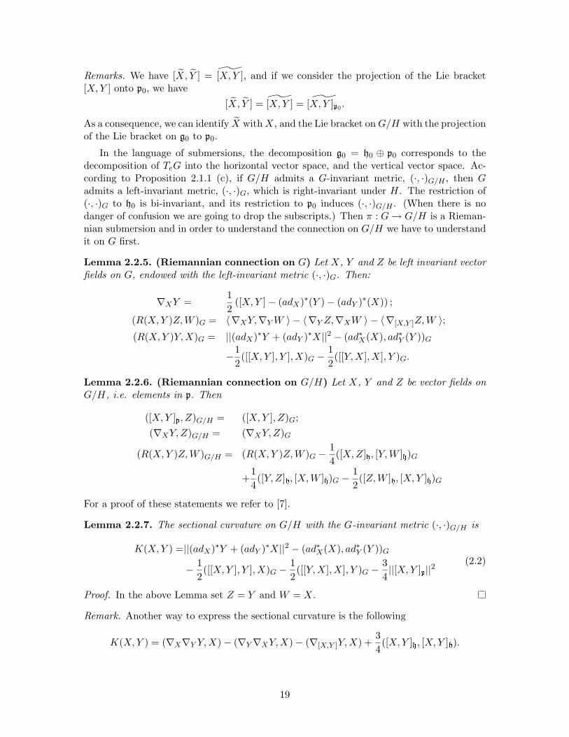
Lemma 2.2.6. (Riemannian connection on G/H) Let X, Y and Z be vector fields onG/H, i.e. elements in p. Then

([X, Y ]p, Z)G/H = ([X, Y ], Z)G;(∇XY, Z)G/H = (∇XY,Z)G

(R(X, Y )Z, W )G/H = (R(X,Y )Z,W )G − 14([X,Z]h, [Y,W ]h)G

+14([Y, Z]h, [X, W ]h)G − 1

2([Z,W ]h, [X, Y ]h)G

For a proof of these statements we refer to [7].

Lemma 2.2.7. The sectional curvature on G/H with the G-invariant metric (·, ·)G/H is

K(X,Y ) =||(adX)∗Y + (adY )∗X||2 − (ad∗X(X), ad∗Y (Y ))G

− 12([[X, Y ], Y ], X)G − 1

2([[Y, X], X], Y )G − 3

4||[X, Y ]p||2

(2.2)

Proof. In the above Lemma set Z = Y and W = X.

Remark. Another way to express the sectional curvature is the following

K(X, Y ) = (∇X∇Y Y, X)− (∇Y∇XY,X)− (∇[X,Y ]Y, X) +34([X, Y ]h, [X,Y ]h).

19

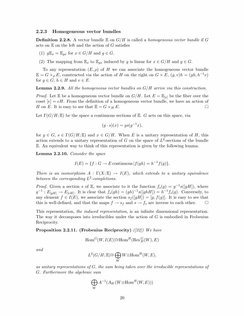
2.2.3 Homogeneous vector bundles

Definition 2.2.8. A vector bundle E on G/H is called a homogeneous vector bundle if Gacts on E on the left and the action of G satisfies

(1) gEx = Egx for x ∈ G/H and g ∈ G.

(2) The mapping from Ex to Egx induced by g is linear for x ∈ G/H and g ∈ G.

To any representation (E, ρ) of H we can associate the homogeneous vector bundleE = G ×ρ E, constructed via the action of H on the right on G × E, (g, v)h = (gh, h−1v)for g ∈ G, h ∈ H and v ∈ E.

Lemma 2.2.9. All the homogeneous vector bundles on G/H arrive via this construction.

Proof. Let E be a homogeneous vector bundle on G/H. Let E = E[e] be the fiber over thecoset [e] = eH. From the definition of a homogeneous vector bundle, we have an action ofH on E. It is easy to see that E = G×H E.

Let Γ(G/H;E) be the space a continuous sections of E. G acts on this space, via

(g · s)(x) = gs(g−1x),

for g ∈ G, s ∈ Γ(G/H;E) and x ∈ G/H. When E is a unitary representation of H, thisaction extends to a unitary representation of G on the space of L2-sections of the bundleE. An equivalent way to think of this representation is given by the following lemma.

Lemma 2.2.10. Consider the space

I(E) = f : G → E continuous |f(gh) = h−1f(g).

There is an isomorphism A : Γ(X;E) → I(E), which extends to a unitary equivalencebetween the corresponding L2-completions.

Proof. Given a section s of E, we associate to it the function fs(g) = g−1s([gH]), whereg−1 : E[gH] → E[eH]. It is clear that fs(gh) = (gh)−1s([ghH]) = h−1fs(g). Conversely, toany element f ∈ I(E), we associate the section sf ([gH]) = [g, f(g)]. It is easy to see thatthis is well-defined, and that the maps f → sf and s → fs are inverse to each other.

This representation, the induced representation, is an infinite dimensional representation.The way it decomposes into irreducibles under the action of G is embodied in FrobeniusReciprocity.

Proposition 2.2.11. (Frobenius Reciprocity) ([22]) We have

HomG(W, I(E))∼=HomH(Res GH(W ), E)

andL2(G/H;E)∼=

⊕

W

W⊗HomH(W,E),

as unitary representations of G, the sum being taken over the irreducible representations ofG. Furthermore the algebraic sum

⊕

W

A−1(AW (W⊗HomH(W,E)))

20

is dense in Γ(X;E) relative to the uniform topology. Here AW is the induced map

AW : W⊗HomH(W,E) → I(E),

defined by AW (w⊗P )(g) = P (g−1w).

Note that the action of G on I(E), translates at the level of AW into g (AW (w⊗P )) =AW (πW (g)w⊗P ). Here, Res G

H(W,π) denotes the representation of H induced via restrictionfrom the representation of G, (W,π).

2.2.4 Homogeneous Differential operators

Definition 2.2.12. Let E and F be homogeneous vector bundles on G/H. A differentialoperator D : Γ∞(G/H;E) → Γ∞(G/H;F) is called a homogeneous differential operator ifg · (Ds) = D(g · s) for g ∈ G and s ∈ Γ∞(G/H;E).

On homogeneous spaces we had special kind of vector bundles, the homogeneous vectorbundles which are in 1−1 correspondence to the representations of H. It turns out that thehomogeneous differential operators have also a description in terms of the representationtheory.

Lemma 2.2.13. Any homogeneous differential operator of order m corresponds to an ele-ment in

(Hom(E, F )⊗Um(g))H .

2.3 Spin structures and Dirac operators on Homogeneousmanifolds

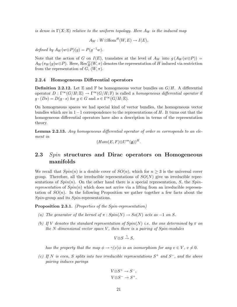
We recall that Spin(n) is a double cover of SO(n), which for n ≥ 3 is the universal covergroup. Therefore, all the irreducible representations of SO(N) give us irreducible repre-sentations of Spin(n). On the other hand there is a special representation, S, the Spin-representation of Spin(n) which does not arrive via a lifting from an irreducible represen-tation of SO(n). In the following Proposition we gather together a few facts about theSpin-group and its Spin-representations.

Proposition 2.3.1. (Properties of the Spin-representation)

(a) The generator of the kernel of π : Spin(N) → So(N) acts as −1 on S.

(b) If V denotes the standard representation of Spin(N) i.e. the one determined by π onthe N -dimensional vector space V , then there is a pairing of Spin-modules

V⊗Sγ→ S,

has the property that the map φ → γ(v)φ is an isomorphism for any v ∈ V , v 6= 0.

(c) If N is even, S splits into two irreducible representations S+ and S−, and the abovepairing induces parings

V⊗S+ → S−,

V⊗S− → S+.

21

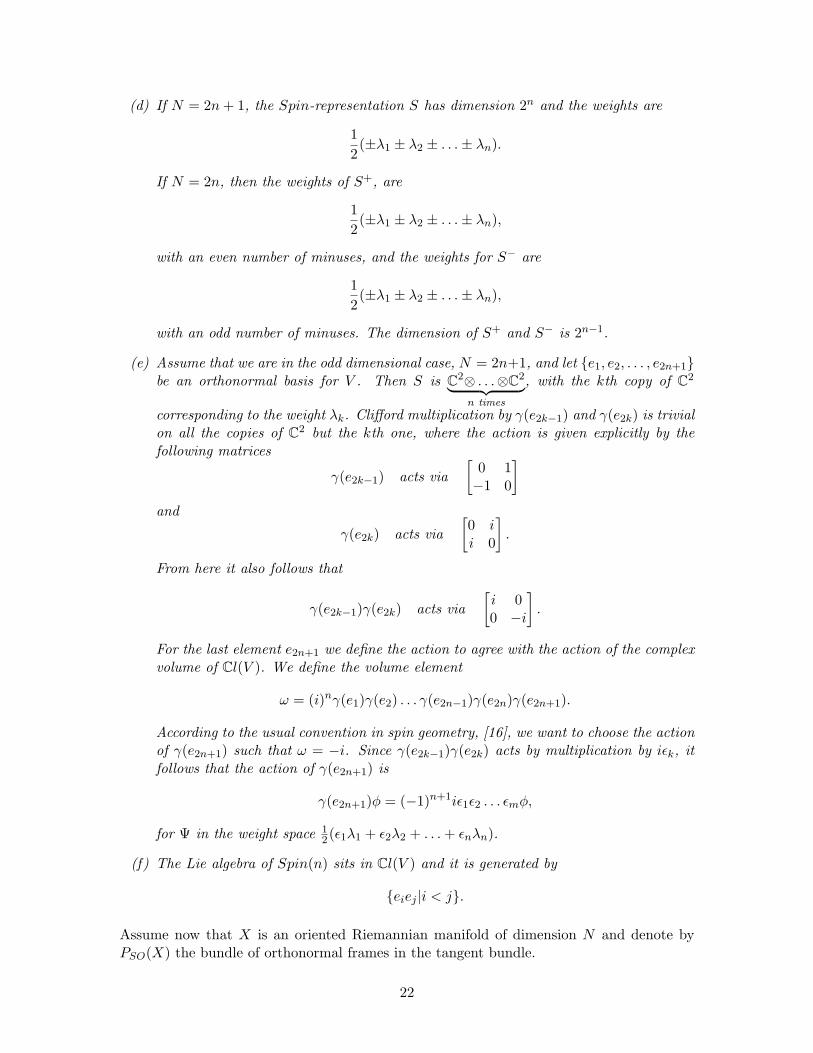
(d) If N = 2n + 1, the Spin-representation S has dimension 2n and the weights are

12(±λ1 ± λ2 ± . . .± λn).

If N = 2n, then the weights of S+, are

12(±λ1 ± λ2 ± . . .± λn),

with an even number of minuses, and the weights for S− are

12(±λ1 ± λ2 ± . . .± λn),

with an odd number of minuses. The dimension of S+ and S− is 2n−1.

(e) Assume that we are in the odd dimensional case, N = 2n+1, and let e1, e2, . . . , e2n+1be an orthonormal basis for V . Then S is C2⊗ . . .⊗C2

︸ ︷︷ ︸n times

, with the kth copy of C2

corresponding to the weight λk. Clifford multiplication by γ(e2k−1) and γ(e2k) is trivialon all the copies of C2 but the kth one, where the action is given explicitly by thefollowing matrices

γ(e2k−1) acts via[

0 1−1 0

]

and

γ(e2k) acts via[0 ii 0

].

From here it also follows that

γ(e2k−1)γ(e2k) acts via[i 00 −i

].

For the last element e2n+1 we define the action to agree with the action of the complexvolume of Cl(V ). We define the volume element

ω = (i)nγ(e1)γ(e2) . . . γ(e2n−1)γ(e2n)γ(e2n+1).

According to the usual convention in spin geometry, [16], we want to choose the actionof γ(e2n+1) such that ω = −i. Since γ(e2k−1)γ(e2k) acts by multiplication by iεk, itfollows that the action of γ(e2n+1) is

γ(e2n+1)φ = (−1)n+1iε1ε2 . . . εmφ,

for Ψ in the weight space 12(ε1λ1 + ε2λ2 + . . . + εnλn).

(f) The Lie algebra of Spin(n) sits in Cl(V ) and it is generated by

eiej |i < j.

Assume now that X is an oriented Riemannian manifold of dimension N and denote byPSO(X) the bundle of orthonormal frames in the tangent bundle.

22

Definition 2.3.2. A Spin-structure on X is a principal Spin(N)-bundle PSpin(X) whichis a double cover of PSO(X) such that the fiberwise restriction πx : Spin(N)x → SO(N)x

is isomorphic to the standard map π : Spin(N) → SO(N) π : Spin(N) → SO(N).

The property of a manifold to admit a Spin-structure is a topological property, and we have

Proposition 2.3.3. The orientable Riemannian manifold admits a Spin-structure in andonly if the second Stiefel-Whitney class of X, w2(X), is zero. Furthermore, if w2(X) = 0,then the distinct Spin-structures on X are in one-to-one correspondence with the elementsof H1(X;Z2).

In the case X is the homogeneous manifold G/H, equipped with a G-invariant Rieman-nian metric, we have an action of G on PSO(X) which makes this bundle G-equivariant.We look at the possible Spin-structures which are compatible with the G-action. We willcall such a Spin-structure a G-equivariant Spin-structure.

Lemma 2.3.4. The homogeneous manifold G/H endowed with the G-invariant metric (·, ·),admits a G-invariant Spin-structure if and only if the adjoint representation Ad : H →SO(p0), admits a lifting Ad to Spin(p)

Spin(N)

π

²²H

fAd;;vvvvvvvvv Ad // SO(N)

.

Remark. First of all, for a homogeneous manifold G/H to admit a G-equivariant Spin-structure, we need it to be Spin. This is a topological condition: w2(G/H) = 0. Then, weneed a G-equivariant Spin-structure. This might exist or might not exists. For example, theodd-dimensional sphere S2n−1 can be viewed as the homogeneous space SU(n)/SU(n− 1),which admits an SU(n)-equivariant Spin-structure since SU(n−1) is simply-connected andthe lifting of the adjoint representation is possible. But, if we view it as the homogeneousspace U(n)/U(n− 1), then it does not admit a U(n)-equivariant Spin-structure.

For the time being, we assume that the homogeneous space G/H admits a G-equivariantSpin-structure.

Since rankH + r = rankG, the dimension of p0 is either odd or even, depending on theparity of r. In this paper we are concerned with the case dim (p0) is odd, which meansthat there is only one irreducible representation of Spin(p0), σ : Spin(p0) → End(S).Therefore, we must assume that r is odd-dimensional, which translates into dim (t0 ∩ p0)is odd-dimensional. Denote the dimension of p0 by 2n + 1, and fix e1, e2, . . . , e2n+1 anorthonormal basis of p0 with respect our chosen G-invariant inner-product.

We choose a maximal torus in SO(p0) such that it extends the torus, ad(TK), inducedby the adjoint representation. The weights of the standard representation of SO(p) on pCare of the form ±λ1,±λ2, . . . ,±λn, 0, where λi are the simple roots of SO(p). In theseterms, the weights of (S, σ) are given by

12

(±λ1 ± λ2 ± . . .± λn) .

Via the lifting Ad, S become the H-module (S, σ Ad).

23

Lemma 2.3.5. Let Y ∈ h. Then

ad(Y ) =2n+1∑

a,b=1

([Y, ea], eb)4

eaeb,

where ad is the differential of Ad at e ∈ H, the identity element.

Proof. For any element z ∈ p let X(z) : Cl(p0) → Cl(p0) be the linear map

x → zx− xz, , for x ∈ Cl(p0).

It is clear that

X(eaeb)(ec) =

0 if c 6= a, b2eb if c = a

− 2ea if c = b(2.3)

It follows that for z ∈ spin(p0), X(z)(p0) ⊂ p0. Thus X(z) restricts to an endomorphismof p, which we will also denote by X(z). For Y ∈ h, we have

X(ad(Y )) = adY,

when acting on p0. The standard basis for spin(p0) is ea · eb|1 ≤ a < b ≤ 2n + 1. In thisbasis

ad(Y ) =∑

1≤a<b≤2n+1

Aab eaeb,

and our job is to compute the coefficients Aab. We have

[Y, ec] =∑

a<b

Aab X(eaeb) ec

=∑

c<b

2Acb eb −∑a<c

2Aab ea,(2.4)

and therefore([Y, ea], eb) = 2Aab for a < b.

It follows thatad(Y ) =

∑

a<b

([Y, ea], eb)2

eaeb.

Using the fact that for a = b we have

([Y, ea], ea) = 0,

and that([Y, ea], eb) eaeb = ([Y, eb], ea) ebea,

the conclusion of the Lemma follows.

2.3.1 The Dirac operator

We assume that there is a lifting of Ad : H → SO(p0) to Ad : H → Spin(p0), so that Sbecomes an H-module. Since the Dirac operator is canonically associated to the metric and

24

the Spin-structure, it follows that it will be G-invariant.Because of Frobenius Reciprocity, the space of spinors has the following decomposition

under the action of GΩ0(G/H,S) =

⊕

V

V⊗HomH(V, S). (2.5)

The Dirac operator is a homogeneous differential operator.

Lemma 2.3.6. Via Frobenius Reciprocity, the Dirac operator becomes a morphism in thecategory of G-modules. In particular, restricted to each of the isotopic components, it hasthe form

DV (w⊗P ) = w⊗γ(ea)∇Spinea

⊗1− w⊗γ(ea)P (πV (ea)). (2.6)

Proof. Denote by Φw⊗P the spinor defined via Φw⊗P (g) = AV (w⊗P )(g) = P (g−1w).

DV (w⊗P )(g) = DΦw⊗P (g)

=∑

γ(ea)∇spinea

Φw⊗P (g)

=∑

γ(ea)∇spinea

(fαΨα)(g)

=∑

γ(ea)((ea(fα)Ψalpha) + fα∇spin

eaΨalpha

)(g)

= −∑

γ(ea)P (πV (ea)g−1w) + w⊗(∑

γ(ea)∇spinea

P )(g)

= −∑

w⊗γ(ea)PπV (ea) + w⊗(∑

γ(ej)∇spinea

P )(g)

An alternative way to think of this (which is going to be used when we actually do compu-tations) is to consider the space of spinors as being

Ω0(G/H,S) = (S⊗C∞(G))H , (2.7)

which can be spelled out as taking the space of smooth maps from G to S, and consideringthe H-invariant ones. The correspondence between the two interpretations is pretty obvious.

There is an action of gC on C∞(G), the space of smooth complex valued functions onG, defined as

π(X)f = X(f),

for any X ∈ gC and f ∈ C∞(G). The action of g on C∞ induces an action of g on the spaceof spinors. In the description of the space of spinors given by (2.7), the action is

π(X)(Φ⊗f) = Φ⊗π(X)f,

where Φ ∈ S and f ∈ C∞(G) such that Φ⊗f is a spinor on G/H, i.e. Φ⊗f(S⊗C∞(G))H .Under the action of G the space of spinors decomposes as

Ω0(G/H,S) = (∑

V

V⊗V ∗⊗S)H

=∑

V

V⊗(V ∗⊗S)H ,(2.8)

where V is an irreducible representation of G and (V ∗⊗S)H represents the multiplicity of

25

the irreducible representation V in the decomposition of the space of spinors under theaction of G. The Dirac operator is a G-equivariant operator and therefore it preserves thedecomposition (2.8). On each of the isotopic components, we can look at

DV : V⊗(V ∗⊗S)H → V⊗(V ∗⊗S)H ,

which is an endomorphism of finite dimensional vector spaces. It turns out that the Diracoperator really acts on the (V ∗⊗S)H part, and the way it acts is given by the followinglemma.

Lemma 2.3.7. The map

DV (w⊗Ψ) = w⊗(∑

a

(γ(ea)∇Spinea

⊗1)Ψ +∑

a

(γ(ea)⊗π(ea))Ψ

)(2.9)

where Ψ ∈ (V ∗⊗S)H , w ∈ V and ∇spinea acts on S via −1

4γ(∇eaeb)γ(eb).

Therefore, in order to compute the spectrum of the Dirac operator, we need to compute itfor each DV . From the expression of DV , it turns out that the eigenspaces are all going tobe sums of copies of V . The number of copies and the eigenvalue is a hard computation,and we are able to perform it in the next chapter in the case of the odd-dimensional sphere,viewed as a homogeneous space.

26

Chapter 3

The case of the odd-dimensionalsphere

In this chapter we analyze the spectrum of the Dirac operator on S2n−1. If we view S2n−1

as the homogeneous space U(n)/U(n− 1), there is no U(n)-invariant Spin-structure on it.

Rather we have to consider the double covers U(n) and ˜U(n− 1).

3.1 Invariant Spin-structures on S2n−1

If we consider the Lie algebra u(N), the simply-connected Lie group with this Lie algebrais SU(N)×S1. The smallest Lie group which has this Lie algebra is U(N). U(N) arises asa quotient of SU(N)× S1 modulo a discrete group (of the center of SU(N)× S1):

1 → Ker(ρ) → SU(N)× S1 ρ→ U(N) → 1,

where ρ(g, eiθ) = eiθ · g. Therefore Ker(ρ) is generated by elements of the form

(e2πiN · I, e−

2πiN ).

The fundamental group of U(N) is Z.If we consider the sphere as the homogeneous space U(n)/U(n− 1), then the restriction

of the adjoint map Ad : U(n− 1) → SO(2n− 11) does not lift to Spin(2n− 1), because theimage of the fundamental group of U(n−1), Ad∗π1(U(n−1), I) into the fundamental groupof SO(2n − 1) is actually Z2. Therefore, in order to satisfy the conditions of the LiftingTheorem [18], we have to kill the 2-torsion in the fundamental group of U(n− 1). For this,

we are led to consider the double covers of U(n) and U(n − 1), U(n) and ˜U(n− 1). Theconstruction is illustrated by the following diagram:

˜U(n− 1)

²²

// U(n)

²²

// Spin(2n)

π

²²U(n− 1) // U(n) // SO(2n)

,

where U(n) and ˜U(n− 1) denote the pull-back of Spin(2n).

27

We consider the sphere as the homogeneous space U(n)/ ˜U(n− 1).

Lemma 3.1.1. There is an U(n)-invariant Spin-structure on S2n−1.

We start by analyzing the U(n)-invariant metrics on S2n−1. Denote the basis for theCartan algebra of u(n), tn, by x1, x2, . . . , xn. We think of xj as the matrix with entry1 on the (j, j)-position. With respect this basis, the roots are xj − xk. We choose thefundamental Weyl chamber to be x1 > x2 > . . . > xn >. With respect this notion ofpositivity, the positive roots are ∆+

n = xj − xk|1 ≤ j < k ≤ n, and we choose the simpleroots to be Πn = x1 − x2, . . . , xn−2 − xn−1, xn−1 − xn. We are going to view the Cartanalgebra of u(n − 1), tn−1, as a subalgebra of tn generated by x1, . . . , xn−1. Everything wediscussed about above restricts to u(n− 1):

the roots are xj − xk, with 1 ≤ j, k ≤ n− 1,

positive roots are ∆+n−1 = xj − xk|1 ≤ j < k ≤ n− 1,

the simple roots are Πn−1 = x1 − x2, . . . , xn−2 − xn−1.

Following the notations we introduced in Chapter 2, an Ad( ˜U(n− 1))-invariant complementof u(n− 1) in u(n) is

p = tp ⊕n−1⊕

i=1

(gxi−xn ⊕ g−xi+xn), (3.1)

where tp is 1-dimensional, generated by Hλ, for λ =∑n−1

i=1 (xi − xn).Remark. The only freedom in the choice of p is given by the choice of tp. Our present choiceis suitable with the the decomposition of u(n) into the center and the semi-simple part, andit has the advantage that it will also give an answer to the same question for the sphere asthe homogeneous space SU(n)/SU(n− 1). Another choice is Hxn , for example.From Lemma 2.2.4, it follows that the decomposition of p into irreducible representationsof ˜U(n− 1) is

p = tp ⊕ pxn−1−xn ,

where pxn−1−xn = ⊕n−1j=1 (gxj−xn + g−xj+xn).

Remark. Note that tp is the trivial representation of ˜U(n− 1), and the highest weight ofthe irreducible representation pxn−1−xn is x1.

According to Lemma 2.2.4 there is a 2-parameter family of U(n)-invariant metrics on S2n−1.Up to homothethy, there is just one parameter family, and we are going to take the constantsC1 = C and Cxn−1−xn = 1. Note that the case C = 1 corresponds to the case of the U(n)-

invariant metric on S2n−1 induced by the Ad(U(n)-invariant metric on U(n).

Lemma 3.1.2. An orthonormal basis for p0 is

Z = − i√(n− 1)(n) C

Hλ,

Xj =1√2(Exj−xn − E−xj+xn),

Yj =1√2(iExj−xn + iE−xj+xn).

28

Proof. It is easy to verify that that they form an orthonormal basis with respect to theU(n)-invariant metric of parameter C.

Lemma 3.1.3. The cosets for the orthonormal basis are

[Z, Xj ] = − 1C

√n

n− 1Yj ,

[Z, Yj ] =1C

√n

n− 1Xj ,

[Xj , Yj ] = iHxj−xn ,

[Xj , Xk] =12(−Exj−xk

−E−xj+xk), for j 6= k,

[Xj , Yk] =12(iExj−xk

− iE−xj+xk), for j 6= k,

[Yj , Yk] =12(−Exj−xk

−E−xj+xk), for j 6= k.

Moreover, [Xj , Xk], [Xj , Yk] and [Yj , Yk] belong to h for j 6= k. When projected onto p0,[Xj , Yj ] is −C

√n

n−1 Z.

Proof. We have

[Z, Xj ] = − 1√2

i√(n− 1)n C

[Hλ, Exj−xn − E−xj+xn ]

= − 1√2

i√(n− 1)n C

(λ(Exj−xn)Exj−xn − λ(E−xj+xn)E−xj+xn

)

= − 1√2

i√(n− 1)n C

n(Exj−xn + E−xj+xn

)

= − 1C

√n

n− 1Yj .

Also,

[Xj , Yj ] =12

[Exj−xn −E−xj+xn , iExj−xn + iE−xj+xn

]

=12

2i [Exj−xn , E−xj+xn ]

= iHxj−xn .

29

The vector [Xj , Yj ] has a component in h and a component in p. Since,

([Xj , Yj ], Z) = (iHxj−xn ,− i√(n− 1)nC

Hλ)

=1

(n− 1)√

nC(Hxj−xn ,Hλ)

= − 1√(n− 1)nC

C2 B(Hxj−xn ,Hλ)

= − C√(n− 1)n

λ(Hxj−xn)

= −C

√n

n− 1,

it follows that the projection onto p is −C√

nn−1 Z.

Lemma 3.1.4. The Riemannian connection associated to the chosen U(n)-invariant metricis

∇ZZ = 0,

∇ZXj = −2− C2

2C

√n

n− 1Yj ,

∇ZYj =2− C2

2C

√n

n− 1Xj ,

∇XjZ =C

2

√n

n− 1Yj ,

∇XjXj = 0,

∇XjYj = −C

2

√n

n− 1Z,

∇YjZ = −C

2

√n

n− 1Xj ,

∇YjXj =C

2

√n

n− 1Z,

∇YjYj = 0.

All the other combinations are 0.

Proof. We sketch the computation for ∇ZXj . From the general formula for a Riemannianconnection we have

(∇ZXj , ξ) =12

(([Z,Xj ], ξ)− ([Xj , ξ], Z)− ([Z, ξ], Z)) ,

where ξ ∈ p. Using Lemma 3.1.3, it follows that ∇ZXj has components just in the direction

30

Yj . And,

(∇ZXj , Yj) =12

(([Z, Xj ], Yj)− ([Xj , Yj ], Z)− ([Z, Yj ], Xj).)

=12

((− 1

C

√n

n− 1Yj , Yj)− (−C

√n

n− 1Z,Z)− (

1C

√n

n− 1Xj , Xj)

)

=12

√n

n− 1

(− 1

C+ C − 1

C

)

= −2− C2

2C

√n

n− 1.

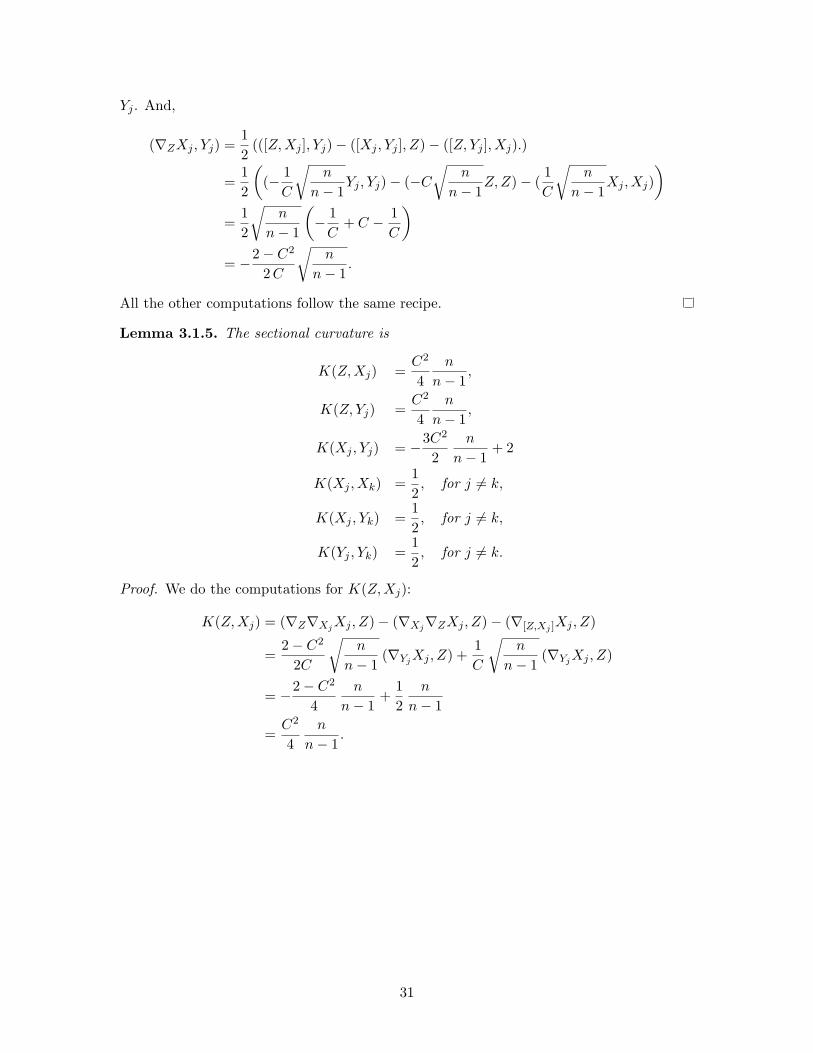
All the other computations follow the same recipe.

Lemma 3.1.5. The sectional curvature is

K(Z,Xj) =C2

4n

n− 1,

K(Z, Yj) =C2

4n

n− 1,

K(Xj , Yj) = −3C2

2n

n− 1+ 2

K(Xj , Xk) =12, for j 6= k,

K(Xj , Yk) =12, for j 6= k,

K(Yj , Yk) =12, for j 6= k.

Proof. We do the computations for K(Z, Xj):

K(Z,Xj) = (∇Z∇XjXj , Z)− (∇Xj∇ZXj , Z)− (∇[Z,Xj ]Xj , Z)

=2− C2

2C

√n

n− 1(∇YjXj , Z) +

1C

√n

n− 1(∇YjXj , Z)

= −2− C2

4n

n− 1+

12

n

n− 1

=C2

4n

n− 1.

31

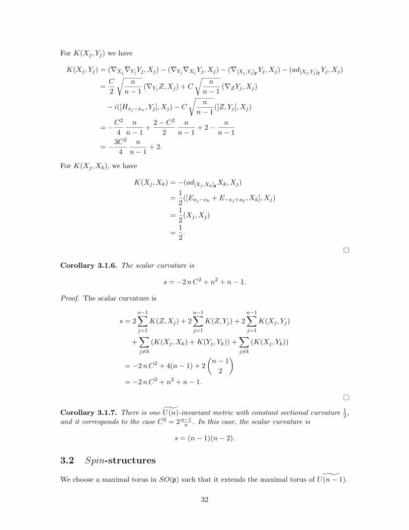
For K(Xj , Yj) we have

K(Xj , Yj) = (∇Xj∇YjYj , Xj)− (∇Yj∇XjYj , Xj)− (∇[Xj ,Yj ]pYj , Xj)− (ad[Xj ,Yj ]hYj , Xj)

=C

2

√n

n− 1(∇YjZ,Xj) + C

√n

n− 1(∇ZYj , Xj)

− i([Hxj−xn , Yj ], Xj)− C

√n

n− 1([Z, Yj ], Xj)

= −C2

4n

n− 1+

2− C2

2n

n− 1+ 2− n

n− 1

= −3C2

4n

n− 1+ 2.

For K(Xj , Xk), we have

K(Xj , Xk) = −(ad[Xj ,Xk]hXk, Xj)

=12([Exj−xk

+ E−xj+xk, Xk], Xj)

=12(Xj , Xj)

=12.

Corollary 3.1.6. The scalar curvature is

s = −2nC2 + n2 + n− 1.

Proof. The scalar curvature is

s = 2n−1∑

j=1

K(Z, Xj) + 2n−1∑

j=1

K(Z, Yj) + 2n−1∑

j=1

K(Xj , Yj)

+∑

j 6=k

(K(Xj , Xk) + K(Yj , Yk)) +∑

j 6=k

(K(Xj , Yk))

= −2n C2 + 4(n− 1) + 2(

n− 12

)

= −2n C2 + n2 + n− 1.

Corollary 3.1.7. There is one U(n)-invariant metric with constant sectional curvature 12 ,

and it corresponds to the case C2 = 2n−1n . In this case, the scalar curvature is

s = (n− 1)(n− 2).

3.2 Spin-structures

We choose a maximal torus in SO(p) such that it extends the maximal torus of ˜U(n− 1).

32

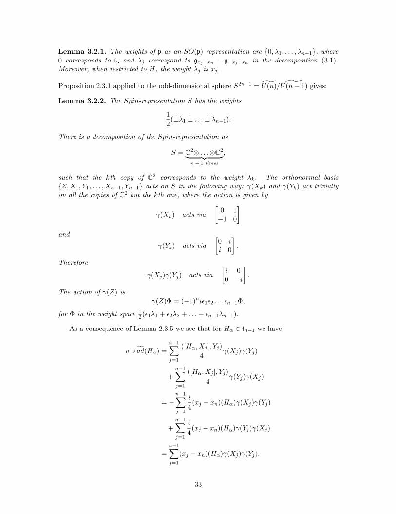
Lemma 3.2.1. The weights of p as an SO(p) representation are 0, λ1, . . . , λn−1, where0 corresponds to tp and λj correspond to gxj−xn − g−xj+xn in the decomposition (3.1).Moreover, when restricted to H, the weight λj is xj.

Proposition 2.3.1 applied to the odd-dimensional sphere S2n−1 = U(n)/ ˜U(n− 1) gives:

Lemma 3.2.2. The Spin-representation S has the weights

12(±λ1 ± . . .± λn−1).

There is a decomposition of the Spin-representation as

S = C2⊗ . . .⊗C2︸ ︷︷ ︸

n− 1 times

,

such that the kth copy of C2 corresponds to the weight λk. The orthonormal basisZ, X1, Y1, . . . , Xn−1, Yn−1 acts on S in the following way: γ(Xk) and γ(Yk) act triviallyon all the copies of C2 but the kth one, where the action is given by

γ(Xk) acts via[

0 1−1 0

]

and

γ(Yk) acts via[0 ii 0

].

Therefore

γ(Xj)γ(Yj) acts via[i 00 −i

].

The action of γ(Z) isγ(Z)Φ = (−1)niε1ε2 . . . εn−1Φ,

for Φ in the weight space 12(ε1λ1 + ε2λ2 + . . . + εn−1λn−1).

As a consequence of Lemma 2.3.5 we see that for Hα ∈ tn−1 we have

σ ad(Hα) =n−1∑

j=1

([Hα, Xj ], Yj)4

γ(Xj)γ(Yj)

+n−1∑

j=1

([Hα, Xj ], Yj)4

γ(Yj)γ(Xj)

= −n−1∑

j=1

i

4(xj − xn)(Hα)γ(Xj)γ(Yj)

+n−1∑

j=1

i

4(xj − xn)(Hα)γ(Yj)γ(Xj)

=n−1∑

j=1

(xj − xn)(Hα)γ(Xj)γ(Yj).

33

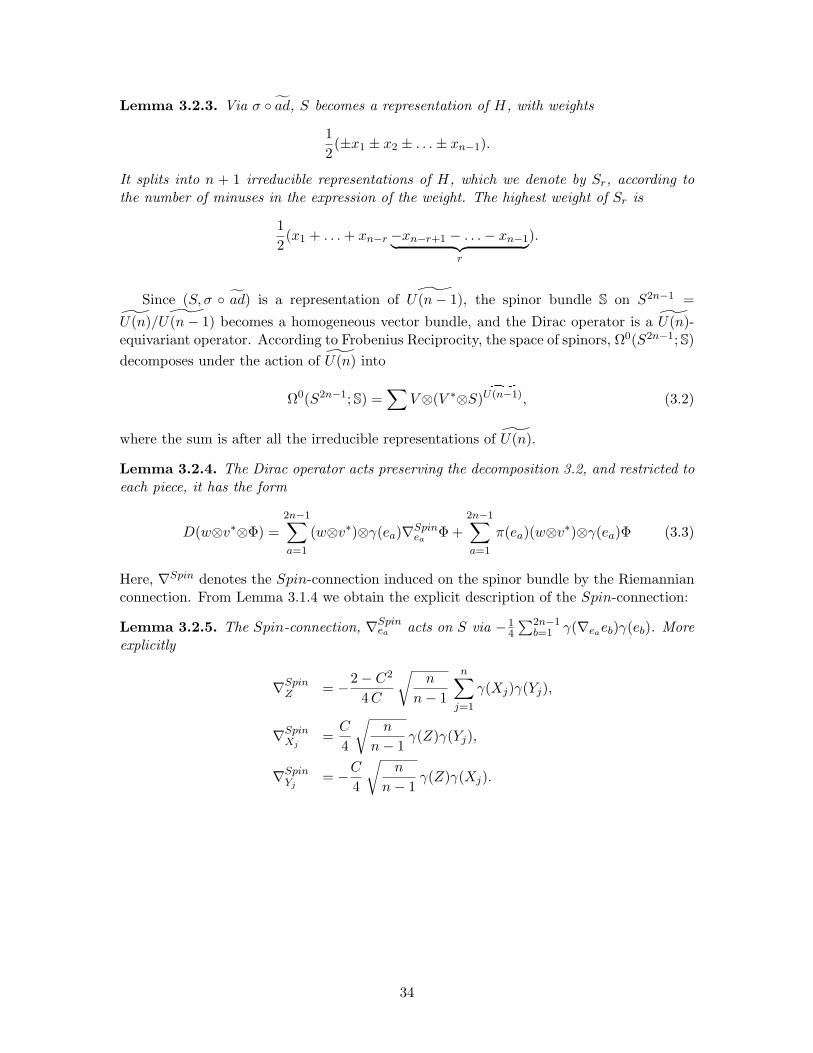
Lemma 3.2.3. Via σ ad, S becomes a representation of H, with weights

12(±x1 ± x2 ± . . .± xn−1).

It splits into n + 1 irreducible representations of H, which we denote by Sr, according tothe number of minuses in the expression of the weight. The highest weight of Sr is

12(x1 + . . . + xn−r −xn−r+1 − . . .− xn−1︸ ︷︷ ︸

r

).

Since (S, σ ad) is a representation of ˜U(n− 1), the spinor bundle S on S2n−1 =

U(n)/ ˜U(n− 1) becomes a homogeneous vector bundle, and the Dirac operator is a U(n)-equivariant operator. According to Frobenius Reciprocity, the space of spinors, Ω0(S2n−1; S)decomposes under the action of U(n) into

Ω0(S2n−1;S) =∑

V⊗(V ∗⊗S)U(n−1), (3.2)

where the sum is after all the irreducible representations of U(n).

Lemma 3.2.4. The Dirac operator acts preserving the decomposition 3.2, and restricted toeach piece, it has the form

D(w⊗v∗⊗Φ) =2n−1∑

a=1

(w⊗v∗)⊗γ(ea)∇Spinea

Φ +2n−1∑

a=1

π(ea)(w⊗v∗)⊗γ(ea)Φ (3.3)

Here, ∇Spin denotes the Spin-connection induced on the spinor bundle by the Riemannianconnection. From Lemma 3.1.4 we obtain the explicit description of the Spin-connection:

Lemma 3.2.5. The Spin-connection, ∇Spinea acts on S via −1

4

∑2n−1b=1 γ(∇eaeb)γ(eb). More

explicitly

∇SpinZ = −2− C2

4C

√n

n− 1

n∑

j=1

γ(Xj)γ(Yj),

∇SpinXj

=C

4

√n

n− 1γ(Z)γ(Yj),

∇SpinYj

= −C

4

√n

n− 1γ(Z)γ(Xj).

34

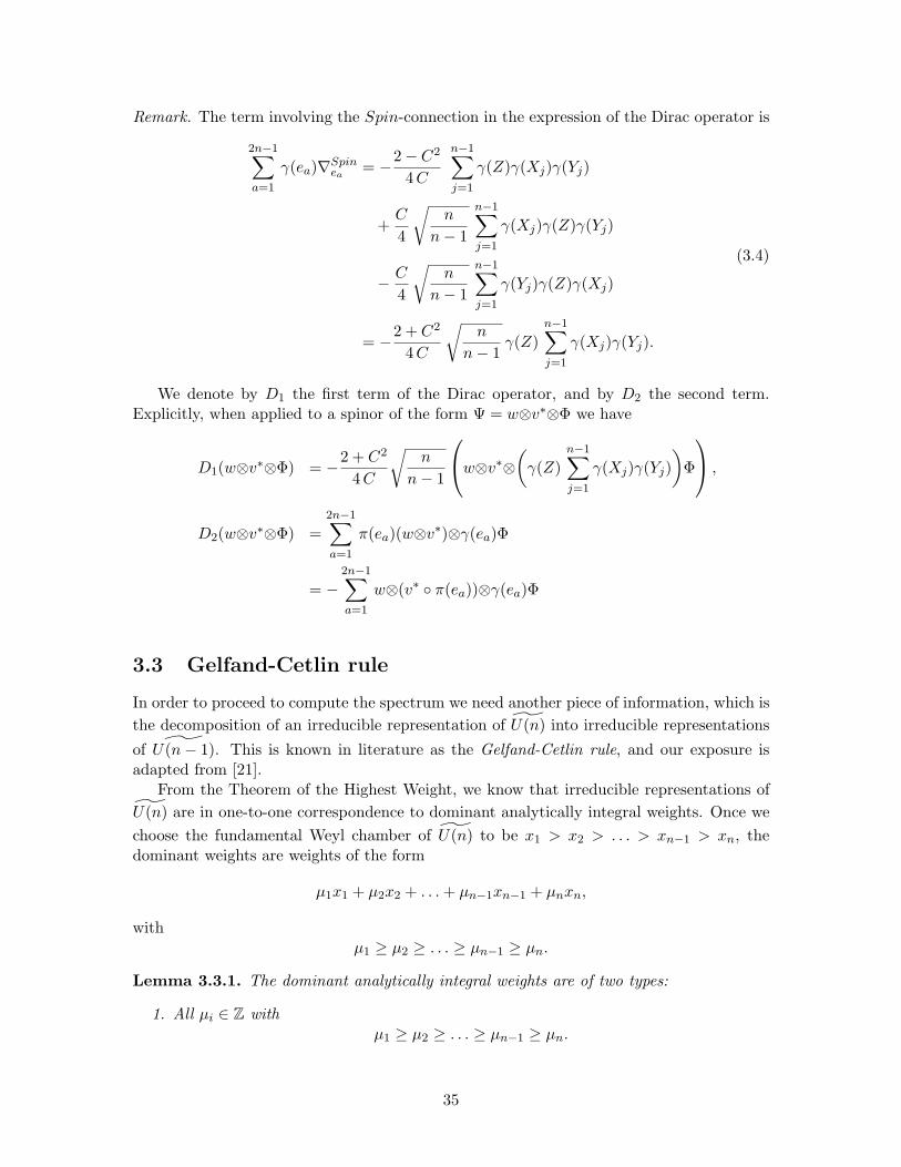
Remark. The term involving the Spin-connection in the expression of the Dirac operator is

2n−1∑

a=1

γ(ea)∇Spinea

= −2− C2

4C

n−1∑

j=1

γ(Z)γ(Xj)γ(Yj)

+C

4

√n

n− 1

n−1∑

j=1

γ(Xj)γ(Z)γ(Yj)

− C

4

√n

n− 1

n−1∑

j=1

γ(Yj)γ(Z)γ(Xj)

= −2 + C2

4C

√n

n− 1γ(Z)

n−1∑

j=1

γ(Xj)γ(Yj).

(3.4)

We denote by D1 the first term of the Dirac operator, and by D2 the second term.Explicitly, when applied to a spinor of the form Ψ = w⊗v∗⊗Φ we have

D1(w⊗v∗⊗Φ) = −2 + C2

4C

√n

n− 1

w⊗v∗⊗

(γ(Z)

n−1∑

j=1

γ(Xj)γ(Yj))

Φ

,

D2(w⊗v∗⊗Φ) =2n−1∑

a=1

π(ea)(w⊗v∗)⊗γ(ea)Φ

= −2n−1∑

a=1

w⊗(v∗ π(ea))⊗γ(ea)Φ

3.3 Gelfand-Cetlin rule

In order to proceed to compute the spectrum we need another piece of information, which isthe decomposition of an irreducible representation of U(n) into irreducible representations

of ˜U(n− 1). This is known in literature as the Gelfand-Cetlin rule, and our exposure isadapted from [21].

From the Theorem of the Highest Weight, we know that irreducible representations ofU(n) are in one-to-one correspondence to dominant analytically integral weights. Once wechoose the fundamental Weyl chamber of U(n) to be x1 > x2 > . . . > xn−1 > xn, thedominant weights are weights of the form

µ1x1 + µ2x2 + . . . + µn−1xn−1 + µnxn,

withµ1 ≥ µ2 ≥ . . . ≥ µn−1 ≥ µn.

Lemma 3.3.1. The dominant analytically integral weights are of two types:

1. All µi ∈ Z withµ1 ≥ µ2 ≥ . . . ≥ µn−1 ≥ µn.

35

These are dominant weights which are analytically integral for U(n) also. They giverepresentations of U(n) which descend to U(n).

2. All µi ∈ Z+ 12 with

µ1 ≥ µ2 ≥ . . . ≥ µn−1 ≥ µn.

These weights are not analytically integral with respect U(n), and −1 ∈ U(n) acts as−Id.

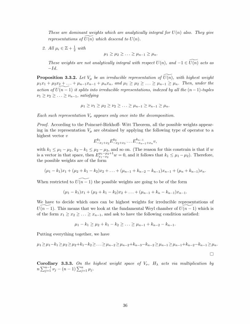
Proposition 3.3.2. Let Vµ be an irreducible representation of U(n), with highest weightµ1x1 + µ2x2 + . . . + µn−1xn−1 + µnxn, and µ1 ≥ µ2 ≥ . . . ≥ µn−1 ≥ µn. Then, under theaction of ˜U(n− 1) it splits into irreducible representations, indexed by all the (n−1)-tuplesν1 ≥ ν2 ≥ . . . ≥ νn−1, satisfying

µ1 ≥ ν1 ≥ µ2 ≥ ν2 ≥ . . . ≥ µn−1 ≥ νn−1 ≥ µn.

Each such representation Vν appears only once into the decomposition.

Proof. According to the Poincare-Birkhoff- Witt Theorem, all the possible weights appear-ing in the representation Vµ are obtained by applying the following type of operator to ahighest vector v

Ek1−x1+x2Ek2−x2+x3

. . . Ekn−1−xn−1+xn

v,

with k1 ≤ µ1 − µ2, k2 − k1 ≤ µ2 − µ3, and so on. (The reason for this constrain is that if wis a vector in that space, then Eµ1−µ2+1

x1−x2w = 0, and it follows that k1 ≤ µ1−µ2). Therefore,

the possible weights are of the form

(µ1 − k1)x1 + (µ2 + k1 − k2)x2 + . . . + (µn−1 + kn−2 − kn−1)xn−1 + (µn + kn−1)xn.

When restricted to ˜U(n− 1) the possible weights are going to be of the form

(µ1 − k1)x1 + (µ2 + k1 − k2)x2 + . . . + (µn−1 + kn − kn−1)xn−1.

We have to decide which ones can be highest weights for irreducible representations of˜U(n− 1). This means that we look at the fundamental Weyl chamber of ˜U(n− 1) which is

of the form x1 ≥ x2 ≥ . . . ≥ xn−1, and ask to have the following condition satisfied:

µ1 − k1 ≥ µ2 + k1 − k2 ≥ . . . ≥ µn−1 + kn−2 − kn−1.

Putting everything together, we have

µ1≥µ1−k1≥µ2≥µ2+k1−k2≥ . . .≥µn−2≥µn−2+kn−3−kn−2≥µn−1≥µn−1+kn−2−kn−1≥µn.

Corollary 3.3.3. On the highest weight space of Vν , Hλ acts via multiplication byn

∑n−1j=1 νj − (n− 1)

∑nj=1 µj.

36

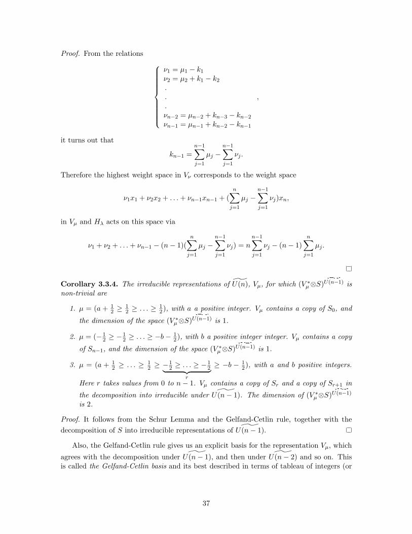
Proof. From the relations

ν1 = µ1 − k1

ν2 = µ2 + k1 − k2

.

.

.νn−2 = µn−2 + kn−3 − kn−2

νn−1 = µn−1 + kn−2 − kn−1

,

it turns out that

kn−1 =n−1∑

j=1

µj −n−1∑

j=1

νj .

Therefore the highest weight space in Vν corresponds to the weight space

ν1x1 + ν2x2 + . . . + νn−1xn−1 + (n∑

j=1

µj −n−1∑

j=1

νj)xn,

in Vµ and Hλ acts on this space via

ν1 + ν2 + . . . + νn−1 − (n− 1)(n∑

j=1

µj −n−1∑

j=1

νj) = nn−1∑

j=1

νj − (n− 1)n∑

j=1

µj .

Corollary 3.3.4. The irreducible representations of U(n), Vµ, for which (V ∗µ⊗S)U(n−1) is

non-trivial are

1. µ = (a + 12 ≥ 1

2 ≥ . . . ≥ 12), with a a positive integer. Vµ contains a copy of S0, and

the dimension of the space (V ∗µ⊗S)U(n−1) is 1.

2. µ = (−12 ≥ −1

2 ≥ . . . ≥ −b− 12), with b a positive integer integer. Vµ contains a copy

of Sn−1, and the dimension of the space (V ∗µ⊗S)U(n−1) is 1.

3. µ = (a + 12 ≥ . . . ≥ 1

2 ≥ −12 ≥ . . . ≥ −1

2︸ ︷︷ ︸r

≥ −b − 12), with a and b positive integers.

Here r takes values from 0 to n− 1. Vµ contains a copy of Sr and a copy of Sr+1 in

the decomposition into irreducible under ˜U(n− 1). The dimension of (V ∗µ⊗S)U(n−1)

is 2.

Proof. It follows from the Schur Lemma and the Gelfand-Cetlin rule, together with thedecomposition of S into irreducible representations of ˜U(n− 1).

Also, the Gelfand-Cetlin rule gives us an explicit basis for the representation Vµ, which

agrees with the decomposition under ˜U(n− 1), and then under ˜U(n− 2) and so on. Thisis called the Gelfand-Cetlin basis and its best described in terms of tableau of integers (or

37

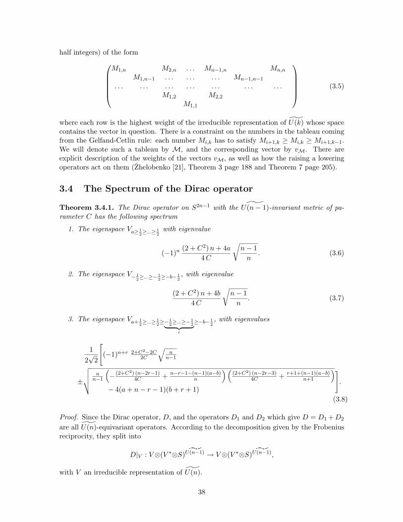
half integers) of the form

M1,n M2,n . . . Mn−1,n Mn,n

M1,n−1 . . . . . . . . . Mn−1,n−1

. . . . . . . . . . . . . . . . . . . . .M1,2 M2,2

M1,1

(3.5)

where each row is the highest weight of the irreducible representation of U(k) whose spacecontains the vector in question. There is a constraint on the numbers in the tableau comingfrom the Gelfand-Cetlin rule: each number Mi,k has to satisfy Mi+1,k ≥ Mi,k ≥ Mi+1,k−1.We will denote such a tableau by M, and the corresponding vector by vM. There areexplicit description of the weights of the vectors vM, as well as how the raising a loweringoperators act on them (Zhelobenko [21], Theorem 3 page 188 and Theorem 7 page 205).

3.4 The Spectrum of the Dirac operator

Theorem 3.4.1. The Dirac operator on S2n−1 with the ˜U(n− 1)-invariant metric of pa-rameter C has the following spectrum

1. The eigenspace Va≥ 12≥...≥ 1

2with eigenvalue

(−1)n (2 + C2)n + 4a

4C

√n− 1

n. (3.6)

2. The eigenspace V− 12≥...≥− 1

2≥−b− 1

2, with eigenvalue

(2 + C2) n + 4b

4C

√n− 1

n. (3.7)

3. The eigenspace Va+ 12≥...≥ 1

2≥− 1

2≥...≥− 1

2︸ ︷︷ ︸r

≥−b− 12, with eigenvalues

12√

2

[(−1)n+r 2+C2−2C

2C

√n

n−1

±√√√√

nn−1

(− (2+C2) (n−2r−1)

4C + n−r−1−(n−1)(a−b)n

)((2+C2) (n−2r−3)

4C + r+1+(n−1)(a−b)n+1

)

− 4(a + n− r − 1)(b + r + 1)

].

(3.8)

Proof. Since the Dirac operator, D, and the operators D1 and D2 which give D = D1 + D2

are all U(n)-equivariant operators. According to the decomposition given by the Frobeniusreciprocity, they split into

D|V : V⊗(V ∗⊗S)U(n−1) → V⊗(V ∗⊗S)U(n−1),

with V an irreducible representation of U(n).

38

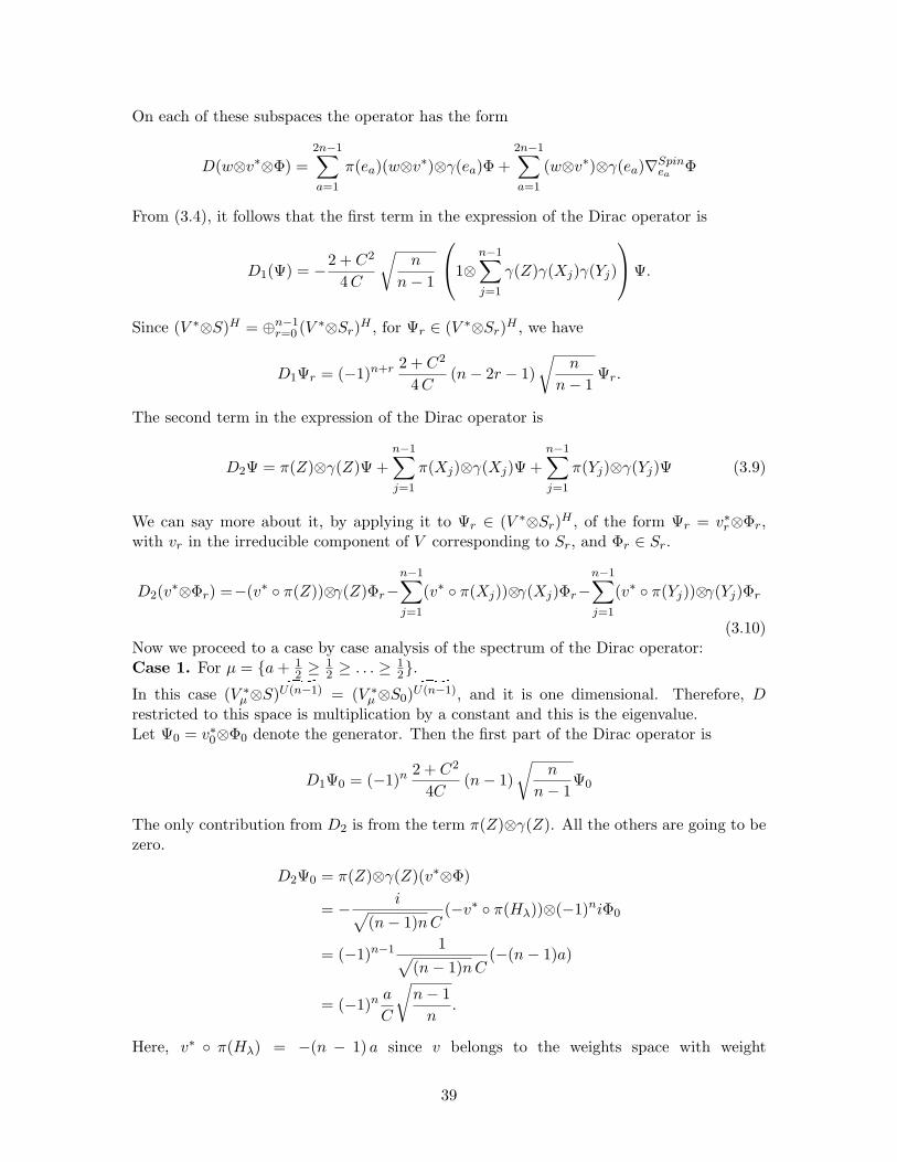
On each of these subspaces the operator has the form

D(w⊗v∗⊗Φ) =2n−1∑

a=1

π(ea)(w⊗v∗)⊗γ(ea)Φ +2n−1∑

a=1

(w⊗v∗)⊗γ(ea)∇Spinea

Φ

From (3.4), it follows that the first term in the expression of the Dirac operator is

D1(Ψ) = −2 + C2

4C

√n

n− 1

1⊗

n−1∑

j=1

γ(Z)γ(Xj)γ(Yj)

Ψ.

Since (V ∗⊗S)H = ⊕n−1r=0 (V ∗⊗Sr)H , for Ψr ∈ (V ∗⊗Sr)H , we have

D1Ψr = (−1)n+r 2 + C2

4C(n− 2r − 1)

√n

n− 1Ψr.

The second term in the expression of the Dirac operator is

D2Ψ = π(Z)⊗γ(Z)Ψ +n−1∑

j=1

π(Xj)⊗γ(Xj)Ψ +n−1∑

j=1

π(Yj)⊗γ(Yj)Ψ (3.9)

We can say more about it, by applying it to Ψr ∈ (V ∗⊗Sr)H , of the form Ψr = v∗r⊗Φr,with vr in the irreducible component of V corresponding to Sr, and Φr ∈ Sr.

D2(v∗⊗Φr) =−(v∗ π(Z))⊗γ(Z)Φr−n−1∑

j=1

(v∗ π(Xj))⊗γ(Xj)Φr−n−1∑

j=1

(v∗ π(Yj))⊗γ(Yj)Φr

(3.10)Now we proceed to a case by case analysis of the spectrum of the Dirac operator:Case 1. For µ = a + 1

2 ≥ 12 ≥ . . . ≥ 1

2.In this case (V ∗

µ⊗S)U(n−1) = (V ∗µ⊗S0)U(n−1), and it is one dimensional. Therefore, D

restricted to this space is multiplication by a constant and this is the eigenvalue.Let Ψ0 = v∗0⊗Φ0 denote the generator. Then the first part of the Dirac operator is

D1Ψ0 = (−1)n 2 + C2

4C(n− 1)

√n

n− 1Ψ0

The only contribution from D2 is from the term π(Z)⊗γ(Z). All the others are going to bezero.

D2Ψ0 = π(Z)⊗γ(Z)(v∗⊗Φ)

= − i√(n− 1)nC

(−v∗ π(Hλ))⊗(−1)niΦ0

= (−1)n−1 1√(n− 1)nC

(−(n− 1)a)

= (−1)n a

C

√n− 1

n.

Here, v∗ π(Hλ) = −(n − 1) a since v belongs to the weights space with weight

39

(12 , . . . , 1

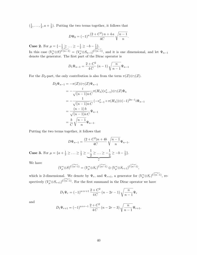
2 , a + 12). Putting the two terms together, it follows that

DΨ0 = (−1)n (2 + C2) n + 4 a

4C

√n− 1

n.

Case 2. For µ = −12 ≥ . . . ≥ −1

2 ≥ −b− 12.

In this case (V ∗µ⊗S)U(n−1) = (V ∗

µ⊗Sn−1)U(n−1), and it is one dimensional, and let Ψn−1

denote the generator. The first part of the Dirac operator is

D1Ψn−1 =2 + C2

4C(n− 1)

√n

n− 1Ψn−1

For the D2-part, the only contribution is also from the term π(Z)⊗γ(Z).

D2Ψn−1 = −π(Z)⊗γ(Z)Ψn−1

= − i√(n− 1)nC

π(Hλ)(v∗n−1)⊗γ(Z)Φn

= − 1√(n− 1)nC

(−v∗n−1 π(Hλ))⊗(−1)2n−1iΨn−1

=(n− 1) b√(n− 1)nC

Ψn−1

=b

C

√n− 1

nΨn−1.

Putting the two terms together, it follows that

DΨn−1 =(2 + C2)n + 4b

4C

√n− 1

nΨn−1.

Case 3. For µ = a + 12 ≥ . . . ≥ 1

2 ≥ −12≥ . . . ≥ −1

2︸ ︷︷ ︸r

≥ −b− 12.

We have(V ∗

µ⊗S)U(n−1) = (V ∗µ⊗Sr)U(n−1) ⊕ (V ∗

µ⊗Sr+1)U(n−1),

which is 2-dimensional. We denote by Ψr, and Ψr+1, a generator for (V ∗µ⊗Sr)U(n−1), re-

spectively (V ∗µ⊗Sr+1)U(n−1). For the first summand in the Dirac operator we have

D1Ψr = (−1)n+r+1 2 + C2

4C(n− 2r − 1)

√n

n− 1Ψr

and

D1Ψr+1 = (−1)n+r−1 2 + C2

4C(n− 2r − 3)

√n

n− 1Ψr+1.

40

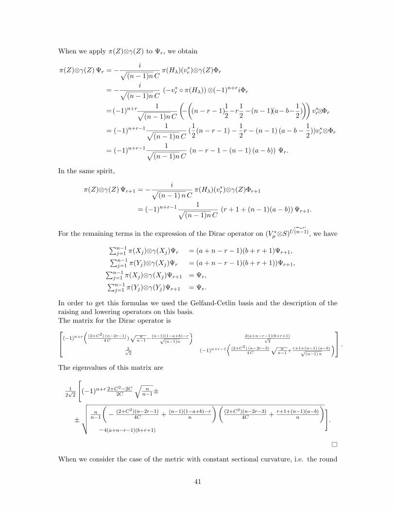
When we apply π(Z)⊗γ(Z) to Ψr, we obtain

π(Z)⊗γ(Z)Ψr = − i√(n− 1)nC

π(Hλ)(v∗r )⊗γ(Z)Φr

= − i√(n− 1)nC

(−v∗r π(Hλ))⊗(−1)n+riΦr

=(−1)n+r 1√(n− 1)nC

(−

((n− r − 1)

12−r

12−(n− 1)(a− b− 1

2)))

v∗r⊗Φr

= (−1)n+r−1 1√(n− 1)nC

(12(n− r − 1)− 1

2r − (n− 1) (a− b− 1

2))v∗r⊗Φr

= (−1)n+r−1 1√(n− 1)nC

(n− r − 1− (n− 1) (a− b)) Ψr.

In the same spirit,

π(Z)⊗γ(Z)Ψr+1 = − i√(n− 1)nC

π(Hλ)(v∗r )⊗γ(Z)Φr+1

= (−1)n+r−1 1√(n− 1)nC

(r + 1 + (n− 1)(a− b))Ψr+1.

For the remaining terms in the expression of the Dirac operator on (V ∗µ⊗S)U(n−1), we have

∑n−1j=1 π(Xj)⊗γ(Xj)Ψr = (a + n− r − 1)(b + r + 1)Ψr+1,∑n−1j=1 π(Yj)⊗γ(Xj)Ψr = (a + n− r − 1)(b + r + 1))Ψr+1,∑n−1

j=1 π(Xj)⊗γ(Xj)Ψr+1 = Ψr,∑n−1j=1 π(Yj)⊗γ(Yj)Ψr+1 = Ψr.

In order to get this formulas we used the Gelfand-Cetlin basis and the description of theraising and lowering operators on this basis.The matrix for the Dirac operator is(−1)n+r

(2+C2) (n−2r−1)

4 C)√

nn−1

− (n−1)(1−a+b)−r√(n−1)n

2(a+n−r−1)(b+r+1)√

2

2√2

(−1)n+r−1

(2+C2) (n−2r−3)

4 C

√n

n−1+

r+1+(n−1) (a−b)√(n−1) n

.

The eigenvalues of this matrix are

12√

2

[(−1)n+r 2+C2−2C

2C

√n

n−1±

±

√√√√√n

n−1

(− (2+C2)(n−2r−1)

4C + (n−1)(1−a+b)−rn

)((2+C2)(n−2r−3)

4C + r+1+(n−1)(a−b)n

)

−4(a+n−r−1)(b+r+1)

].

When we consider the case of the metric with constant sectional curvature, i.e. the round

41

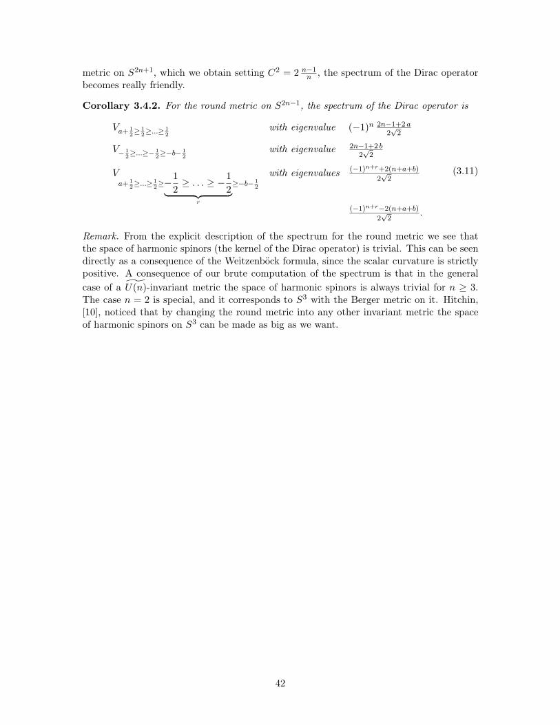
metric on S2n+1, which we obtain setting C2 = 2 n−1n , the spectrum of the Dirac operator

becomes really friendly.

Corollary 3.4.2. For the round metric on S2n−1, the spectrum of the Dirac operator is

Va+ 12≥ 1

2≥...≥ 1

2with eigenvalue (−1)n 2n−1+2 a

2√

2

V− 12≥...≥− 1

2≥−b− 1

2with eigenvalue 2n−1+2 b

2√

2

Va+ 1

2≥...≥ 1

2≥−1

2≥ . . . ≥ −1

2︸ ︷︷ ︸r

≥−b− 12

with eigenvalues (−1)n+r+2(n+a+b)

2√

2

(−1)n+r−2(n+a+b)

2√

2.

(3.11)

Remark. From the explicit description of the spectrum for the round metric we see thatthe space of harmonic spinors (the kernel of the Dirac operator) is trivial. This can be seendirectly as a consequence of the Weitzenbock formula, since the scalar curvature is strictlypositive. A consequence of our brute computation of the spectrum is that in the generalcase of a U(n)-invariant metric the space of harmonic spinors is always trivial for n ≥ 3.The case n = 2 is special, and it corresponds to S3 with the Berger metric on it. Hitchin,[10], noticed that by changing the round metric into any other invariant metric the spaceof harmonic spinors on S3 can be made as big as we want.

42

Chapter 4

The eta-invariant for theodd-dimensional sphere

Definition 4.0.3. For a selfadjoint elliptic operator D on a compact Riemannian manifoldM , the η-function, η(s), is defined as

η(s) =∑

λ∈Σ′(D)

sgn (λ) |λ|−s, (4.1)

for Re(s) > dimM . Here Σ(D) is the spectrum of D and Σ′(D) = Σ(D) \ 0. Moreover, ifa compact group G acts, and D is equivariant with respect to this group action, then theeigenspaces Eλ are finite-dimensional G-modules, and we set

η(g, s) =∑

λ∈Σ′(D)

Trace (g|Eλ) sgn (λ) |λ|−s. (4.2)

These functions were introduced and studied in [1, 2], where it is shown that for a Diractype of operator, η(g, s) has a meromorphic extension to the whole C; one, moreover, whichis holomorphic at zero.

4.1 The untwisted Dirac operator on the sphere

We continue with our set-up from Chapter 3. We consider the odd-dimensional sphere S2n−1

endowed with the round metric. We view it as the homogeneous space U(n)/ ˜U(n− 1), andthe round metric has the property that it is a U(n)-invariant metric. S2n−1 admits a U(n)-invariant Spin-structure. The spectrum of the Dirac operator is given by Corollary 3.4.2.The eigenspaces are representations of U(n), and the goal of this section is to computeη(g, s) for g in U(n). Since U(n) is a compact Lie group, any element g is conjugated to anelement in the maximal torus Tn.

Theorem 4.1.1. For g ∈ Tn, such that 1 is not an eigenvalue, we have

η(g) = (−1)n(det g)12

2det (In − g)

. (4.3)

43

If 1 is an eigenvalue of g, thenη(g) = 0. (4.4)

Remark. Since the function η(g, s) is invariant under the conjugation, the above propositiongives us the entire function η(g, 0) on U(n).

Proof. With the explicit formula for the spectrum, we have to compute 3 sums for theη-function

η1(g, s) = (−1)n∑

a≥0

(2n− 1 + 2a

2√

2

)−s

Trace (g|Va+1

2≥12≥...≥ 1

2

). (4.5)

η2(g, s) =∑

b≥0

(2n− 1 + 2b

2√

2

)−s

Trace (g|V− 12≥...≥− 1

2≥−b− 12

). (4.6)

η3(g, s) =∑

a,b≥0

0≤r≤n−1

((−1)n+r + 2n + 2(a + b)

2√

2

)−s

Trace (g|Va,r,b)

−∑

a,b≥0,

0≤r≤n−1

((−1)n+r−1 + 2(n− 2r − 2) + 2(a + b)

2√

2

)−s

Trace (g|Va,r,b),

(4.7)

where Va,r,b is a shortcut for the irreducible representation of U(n) with highest weightµ = (a + 1

2 ≥ 12 ≥ . . . ≥ 1

2 ≥ −12 ≥ . . . ≥ −1

2︸ ︷︷ ︸r

≥ −b− 12 , We do a case by case analysis of all

these partial η-functions.

Case 1. The representation with highest weight a + 12 ≥ 1

2 ≥ . . . ≥ 12 can be viewed as the

tensor product of two irreducible representations with highest weights a ≥ 0 ≥ . . . ≥ 0 and12 ≥ . . . ≥ 1

2 . The first one, Va≥0≥...≥0, descends to a representation of U(n). Its characteris Hn

a , the ath symmetric polynomial in n variables, i.e. the sum of all distinct monomialsof degree a, [9]. The second representation is half of the determinant representation andits character is the square root of the determinant. With this set up the function η1(g, s)becomes:

η1(g, s) = (−1)n∑

a≥0

(2n− 1 + 2a

2√

2

)−s

det (g)12 Hn

a (g).

Evaluating this expression at s = 0, we obtain

η1(g, 0) = (−1)n det (g)12

∑

a≥0

Hna (g)

= (−1)n det (g)12

1det (In − g)

where for the last equality we used the following identity for symmetric polynomials, [9]:

n∏

i=1

11− xit

=∑

a≥0

Hna ta. (4.8)

44

Case 2. The computations for η2(g, 0) follow the same recipe as for the case of η1(g, 0). Thehalf determinant representation is replaced by the minus half determinant representationand the character of the representation V0≥...≥0≥−b is Hb(g−1). And η2(g, 0) becomes

η2(g, 0) = det (g)−12

1det (In − g−1)

.

Case 3. In the equation (4.7) we see that when we make the s = 0 the entire expressionis convergent. And, in fact it goes to zero. This is because the coefficients in front of thetraces are all going to be one, and all the terms with the same trace appear twice in thesum: once with a positive sign and once with minus. Therefore

η3(g, 0) = 0. (4.9)

Adding up the results of this case-by-case analysis , we obtain

η(g) = (−1)ndet (g)12

1det (In − g)

+ det (g−1)−12

1det (In − g−1)

= (−1)n 2det (In − g)

(det g)12 .

(4.10)

It remains to study the case when g has 1 as an eigenvalue. It is sufficient to study thesituation when 1 is an eigenvalue with multiplicity one. In order to proceed, we need thefollowing resultFact. Consider the Zeta-function

ζ(s, α) =∞∑

k=0

(α + k)−s,

where α is a constant. A consequence of Hermite’s formula, [23], gives the value of the Zetafunction at s = 0

ζ(0, α) =12− α.

With this in mind, we have to compute just the analytical continuations at 0 of η1 and η2.This is because, the argument we used to prove that η3(g, 0) vanishes in the general case,still holds for the case we analyze now.

We assume that the eigenvalues of g are x1, . . . , xn−1, xn. Moreover because g has 1 asan eigenvalue, we can assume that the multiplicity of this eigenvalue is 1, and that xn = 1(the cases where the multiplicity is greater than one, are treated in a similar way). With

45

this,

η1(g, s) = (−1)n(det g)12

∑

a≥0

(2n− 1 + 2a

2√

2

)−s

Hna (x1, . . . , xn−1, xn)

= (−1)n(det g)12

∑

a≥0

(2n− 1 + 2a

2√

2

)−s

Hna (x1, . . . , xn−1, 1)

= (−1)n(det g)12

∑

a≥0

(2n− 1 + 2a

2√

2

)−s a∑

j=0

Hn−1j (x1, . . . , xn−1)

= (−1)n(det g)12 (√

2)s

(∑

a≥0

(2n− 1

2+ a

)−s

Hn−10 (x1, . . . , xn−1)

+∑

a≥1

(2n− 1

2+ a

)−s

Hn−11 (x1, . . . , xn−1) + · · ·+

+∑

a≥k

(2n− 1

2+ a

)−s

Hn−1k (x1, . . . , xn−1) + . . .

).

Using the analytical continuation for the Zeta-function, we obtain

η1(g, 0) = (−1)n(det g)12

∑

k≥0

(12− 2n− 1

2+ k

)Hn−1

k (x1, . . . xn−1)

=(−1)n(det g)12

(

12− 2n− 1

2

)∑

k≥0

Hn−1k (x1, . . . , xn−1)+

∑

k≥0

kHn−1k (x1, . . . , xn−1)

= (−1)n(det g)12

(12− 2n− 1

2

)1

det (In−1 − g′)+

1det (In−1 − g′)

n−1∑

j=0

xj

(1− xj)2

= (−1)n (det g′)12

det (In−1 − g′)

−(n− 1) +

n−1∑

j=0

xj

(1− xj)2

.

Here g′ represents the (n − 1) × (n − 1) matrix with eigenvalues x1, . . . , xn−1, and In−1

represents the identity (n− 1)× (n− 1) matrix. In the same way,

η2(g, 0) =det (g′)−

12

det (In − g′−1)

−(n− 1) +

n−1∑

j=0

x−1j

(1− x−1j )2

= (−1)n−1 det (g′)12

det (In−1 − g′)

−(n− 1) +

n−1∑

j=0

xj

(1− xj)2

.

Since η(g, 0) = η1(g, 0) + η2(g, 0), from these two formulas it follows that

η(g, 0) = 0,

when 1 is an eigenvalue of g.

46

4.2 Orbifold η-invariant

Let Γ be a finite subgroup of SU(n). Since U(n) is a double cover of U(n), which containsSU(n), and therefore Γ, it follows that the structures we defined on S2n−1 (Riemannianmetric, Spin-structure, Dirac operator) are Γ-invariant. We consider the quotient S2n−1/Γ.For almost all the finite groups of SU(n − 1) (except the case n = 2, which correspondsto the lens spaces S3/Γ), the quotient has singularities. Nevertheless, thinking of it as anorbifold, it still makes sense to talk about Spin-structure on it and Dirac operator.

Definition 4.2.1. The orbifold η-invariant is defined to be

η =1|Γ|

∑

γ∈Γ

η(γ). (4.11)

With the explicit formula of the η-character, (4.3), and using the fact that for an elementγ ∈ Γ we have det (γ) = 1, it follows

Corollary 4.2.2. The orbifold η-invariant for S2n−1/Γ is

η = (−1)n∑

γ∈Γ

1 not an eigenvalue for γ

2det (In − γ)

(4.12)

4.3 S1-equivariant η-invariant

The center of U(n), Z, is S1. Since the action of this S1 on S2n−1, commutes with theaction of Γ, we want to consider a S1-equivariant version of the η-invariant.

Definition 4.3.1. The S1-equivariant η-invariant on S2n−1 is

ηS1(t) =

1|Γ|

∑

γ∈Γ

η(tγ), (4.13)

for t ∈ S1, and we view t γ as an element in U(n).

Corollary 4.3.2. The S1-equivariant η-invariant is

ηS1(t) = (−1)nt

n2

∑

γ∈Γ

1det (In − tγ)

. (4.14)

Remark. This formula makes sense, because we view the S1-equivariant η-invariant as anelement in the ring of Laurent polynomials C[[t]].

Proof. It follows from the general formula for η(g, 0), (4.3), applied to g = tγ.

Note. The computation of the S1-equivariant η-invariant is the main reason for which we aredealing with the sphere as the homogeneous space U(n)/ ˜U(n− 1), instead of the straight-forward choice SU(n)/SU(n − 1). The motivation is that, when we look at the orbifoldCn/Γ, there is an action of C∗ by dilations on Cn, which commutes with the action of Γ.Restricted to the boundary, we have the action of S1, the center of U(n). This is the most

47

symmetry we can get in the general case of a finite subgroup of SU(n). In the special caseof a finite abelian subgroup Γ of SU(n), there is extra-symmetry coming from the action of(C∗)n the n-dimensional torus, on Cn/Γ. In this way, the orbifold Cn/Γ becomes a toric va-riety, and this property gives us special techniques to study the geometry of the singularityand its resolutions of singularities.

4.4 Twisted Dirac operator

All we discussed about in the previous sections can be adapted to the case of a twistedDirac operator, by a homogeneous vector bundle E. We know from Chapter 2 that sucha vector bundle if given by a representation, E, of U(n). From Frobenius Reciprocity itfollows that we are going to have the same eigenvalues for the Dirac operator, and thecorresponding eigenspaces are going to be the initial vector spaces tensored with E. Withthis in mind, all the statements and the proofs from the previous section go through withoutany modification, provided that we endowed E with a U(n)-invariant connection. We cancondense everything in the following result.

Proposition 4.4.1. For the Dirac operator associated to the homogeneous vector bundleE,

DE : Ω(S2n−1, S⊗E) → Ω(S2n−1,S⊗E),

the twisted η-character is

ηE(g) =

(−1)n+1(det g)

12

2 χE(g)det (I−g) if 1 is not an eigenvalue of g,

0 if 1 is an eigenvalue of g.(4.15)

Moreover, the twisted orbifold η-invariant on S2n−1/Γ is

ηE = (−1)n 1|Γ|

∑

γ∈Γ

1 not an eigenvalue of γ

2χE(γ)det (In − γ)

(4.16)

and its S1-equivariant version is

ηS1

E (t) = (−1)ntn2

dim CE

|Γ|∑

γ∈Γ

2χE(γ)det (I − tγ)

. (4.17)

48

Chapter 5

Molien series

5.1 Algebraic Geometry Set Up

Let Γ be a finite subgroup of SL(n,C). Consider the set of irreducible representationsR0, R1, . . . , Rp, where R0 stands for the trivial one dimensional representation. There isa natural action of Γ on Cn, and we consider the quotient singularity Cn/Γ. This quotienthas the structure of a complex n + 1-dimensional orbifold.

Its ring of regular functions A[Cn/Γ] is given by the subring

C[X1, X2, . . . , Xn]Γ ⊂ C[X1, X2, . . . , Xn]

of regular functions on Cn which are invariant under the action of Γ. This ring is calledthe ring of invariants. The variety Cn/Γ inherits p + 1 distinct orbifold sheaves Rjp

j=0

consisting of those functions, f(X1, . . . , Xn) on Cn such that

f ∈ C[X1, . . . , Xn]ΓRj,

where C[X1, . . . , Xn]ΓRjis the isotopic component corresponding to Rj in the decomposition

of the ring of polynomials C[X1, . . . , Xn] under the action of Γ, i.e.

C[X1, . . . , Xn] =p⊕

j=0

C[X1, . . . , Xn]ΓRj. (5.1)

Note that C[X1, . . . Xn]ΓR0= C[X1, . . . , Xn]Γ is the space of sections of the orbifold sheaf

R0, which is the structure sheaf of the variety Cn/Γ, OCn/Γ. It follows from the Schur’slemma that each C[X1, . . . , Xn]ΓRj

is a module over the ring of invariants C[X1, . . . ,Cn]Γ,and we call it the module of Rj-relative invariants. Note that this is the same as sayingthat the space of sections of the orbifold sheaf Rj , Γ(Cn/G,Rj), is a module over the ringof regular functions on Cn/Γ.

To simplify the notations we are going to denote by A the ring of polynomials in n-variables, and with this notation the decomposition (5.1) becomes

A = AΓ ⊕ AΓR1

⊕ . . . ⊕ AΓRp

. (5.2)

49

On the polynomial algebra we have a grading given by the degree.

A =⊕

k≥0

An, AkAl ⊂ Ak+l, A0 = C. (5.3)

Since the action of the group Γ preserves this grading, it follows that AΓ has a structure ofa graded algebra,

AΓ =⊕

k≥0

(AΓ ∩Ak) =⊕

k≥0

AΓk ,

and all the other isotopic components, AΓR, have the structure of a graded AΓ-module,

AΓR =

⊕

k≥0

AΓR,k, AΓ

k ·AΓR,l ⊂ AΓ

R,k+l.

We would like to know the dimension of the homogeneous component AΓk , consisting of

Γ-invariant polynomials of degree k, or more generally the dimension of the homogeneouspiece of degree k in AΓ

R. This kind of information is encoded in the Hilbert series (sometimescalled the Poincare series)

p(AΓR, t) =

∞∑

k=0

dim C(AΓR,k) tk.

5.2 Molien series

In this paper we are going to use a modified version of the Hilbert series which is called theMolien series. For a reference, see Stanley’s survey article, [20], and the references therein.

Definition 5.2.1. The Molien series for AΓR is defined to be

ΦR(t) =1

dimR

∑

k≥0

dim C(AΓR,k) tk (5.4)

Corollary 5.2.2. We have∑

R

dim C(R) ΦR(t) = (1− t)−n. (5.5)

Remark. A consequence of the Hilbert-Serre Theorem is that the Molien series is a rationalfunction of t.

The following theorem gives an interpretation of the rational function ΦR(t) in terms of thefinite group.

Theorem 5.2.3. (Molien) Let Γ be a finite subgroup of SL(n,C), and let R be an irre-ducible representation of Γ. Then the Molien series, Φ(AΓ

R, t), of the module of R-relativeinvariants is given by

ΦR(t) =1|Γ|

∑

γ∈Γ

R∗(γ)det (In − tγ)

, (5.6)

where In is the identity matrix and R∗ is the dual character to R.

50

Note. This theorem is valid in the more general case of a finite group of Gl(n,C).

Remark. In the particular case of the ring of invariants, we have

Φ(t) =1|Γ|

∑

γ∈Γ

1|γ| . (5.7)

Corollary 5.2.4. If R is an irreducible representation of Γ,

ΦR(1t) = (−1)n tn ΦR∗(t).

In the particular case R is the trivial representation, this formula becomes

Φ(1t) = (−1)n tn Φ(t).

The following Corollary tells us that all the isotopic components appearing in the decom-position (5.1) are non-trivial.

Corollary 5.2.5. For every irreducible representation R of Γ, the module of R-relativeinvariants, AΓ

R, is non-trivial.

Proof. In the expression (5.6) for ΦR(t), exactly one term, corresponding to γ = In hasa pole of order n at t = 1, while the other terms have poles of order strictly less than n.Therefore ΨR(t) 6= 0, so AΓ

R must be non-trivial.

In the following Proposition we gather together a few results about the structure of thering of invariants, AΓ.

Proposition 5.2.6.

(i) The ring of invariants AΓ has n but not n + 1 algebraically independent invariantsover C. In particular, the Krull dimension of AΓ, dim.Krull(AΓ), is n. Equivalently,dim.Krull(AΓ) is the order to which t = 1 is a pole of the rational function Φ(t).

(ii) AΓ is a Cohen-Macaulay algebra.

(iii) We can always find a homogeneous system of parameters θ1, . . . , θn, with degθi = di,and a set of homogeneous invariants ζ1, . . . , ζp, degζi = ei, such that

AΓ =p⊕

j=1

C[θ1, . . . , θn] ζj .

(iv) The Molien series of the ring of invariants is

Φ(t) =te1 + . . . + tep

(1− td1) . . . (1− tdn). (5.8)

51

(v) If we assume 0 = e1 ≤ e2 ≤ . . . ≤ ep, then

ep =∑n

j=1 (dj − 1) − 1,

ei + ei−p+1 = ep,

p |G| = d1 · d2 · . . . · dn.

Proof. We refer to [20] for a proof. We just sketch the proof of (v) since it uses the Molienseries. From Corollary 5.2.4 and (iv) of the Proposition, we have

Φ(1t

) = (−1)n

p∑

i=1

td1+...+dn−ei

n∏

j=1

(1− tdj )

= (−1)n tn Φ(t),

This implies thatp∑

i=1

td1+...+dn−ei =p∑

i=1

tm+ei .

Because of the order we have on the ei’s, it follows that

d1 + . . . + dn − ei = m + ep−i+1,

for all 1 ≤ i ≤ p. In particular, for i = 1 we obtain

ep =n∑

j=1

dj − n,

and therefore the first relation. Plugging this into the equation for general i, we obtain thesecond relation.For the last relation, we notice that since

Φ(t) =te1 + . . . + tep

(1− td1) . . . (1− tdn),

then the coefficient of the pole at t = 1 of the Molien series is

p

d1 · . . . · dn.

On the other hand, from Molien’s theorem, it follows that the coefficient of the pole att = 1 is coming from the contribution of the identity, and it is 1

|G| . Therefore the thirdrelation.

We have similar results for the module of R-relative invariants. First of all we need todefine the notion of Krull dimension for the module of R-relative invariants. Proposition5.2.6 tells us how to define it.

52

Definition 5.2.7. We define the Krull dimension of the module of R-relative invariants,dim.KrullAΓ

R, to be the order to which t = 1 is a pole of ΦR(t).

Proposition 5.2.8. Let R be an irreducible representation of Γ, and consider the moduleof R-relative invariants AΓ

R.

(i) The Krull dimension of AΓR is n.

(ii) AΓR is a Cohen-Macaulay module.

(iii) AΓR is a finitely generated AΓ-module. Moreover, AΓ

R is generated by homogeneouspolynomials of degree not exceeding |G|, ρ1, . . . ρr

AΓR =

r⊕

i=1

C[θ1, . . . , θn] ρi

5.3 The relation between the η-invariant and the Molien se-ries

The set up is the following: Γ finite subgroup of SU(n), and let R be an irreducible rep-resentation of Γ. There is a natural action of Γ on Cn. To the algebraic variety Cn/Γ weassociate the Molien series of R-relative invariants ΦR(t). To the boundary, S2n−1/Γ, ofthe geometric orbifold ICn/Γ we associate the η-invariant ηR(t). All we had built up untilnow, allows us to state the following nice result which relates the algebraic and geometricalside of the quotient singularity Cn/Γ.

Theorem 5.3.1. The η-invariant is related to the Molien series by the following relation

ηR(t) =(−1)n

2Res 1

ΦR∗(t)1− t

, (5.9)

where R is the dual representation to R.

Remark. If we consider the S1-equivariant η-invariant, ηS1

R (t), then this is related to theMolien series via

ηS1

R (t) = 2 (−1)n tn2 dim C(R) ΦR∗(t). (5.10)

We can further describe the Molien series in terms of η-invariants associated to thesingularity. Consider the Laurent expansion about t = 1 of the Molien series ΦR(t):

ΨR(t) =BR

n

(1− t)n+

BRn−1

(1− t)n−1+ · · ·+ BR

1

1− t+ θR(t). (5.11)

From Molien’s Theorem it is easy to notice that

BRn =

1|G| ,

for any R irreducible representation of Γ. Also, Theorem 5.3.1 implies that

θR(1) =(−1)n

2Res 1

ΦR(t)(1− t)

.

53

Now, the coefficient BRn−1 is given by the following result:

Proposition 5.3.2. Let Γ be a finite subgroup of Sl(n,C). The coefficient BRn−1 in the

Laurent expansion of ΦR(t) at t = 1 is 0 for all irreducible representations R of Γ.

Proof. We consider the Molien series ΦR(t) and we subtract the contribution from theidentity. The remaining expression has a pole of order at most n at t = 1. An elementγ ∈ Γ contributes to this pole if and only if it fixes a subspace of Cn of dimension n − 1.This is because such an element which contributes to the pole of order n − 1 must havethe eigenvalue 1 with multiplicity n− 1. But since we are dealing with a finite subgroup ofSl(n,C), there are no elements with such a property.

Remark. If we drop the assumption that the finite group sits in SL(n,C), and we considerit as a finite group of GL(n,C), then this coefficient is not going to be zero. An element1 6= γ with the property that it fixes a subspace of Cn of dimension n − 1 it is calledpseudoreflection. Let λ be the eigenvalue which is not zero. Then

1det (I − gt)

=1

(1− t)n−1(1− λt),

and after multiplying by (1− t)n−1, the value at t = 1 is 11−λ . We observe that

11− λ

+1

1− λ−1= 1.

So if we pair together each element with its inverse, we see that the total contribution fromall the pseudoreflections is equal to one half of the number of them. Self-inverse elementshave λ = −1, so their contribution is also one half. Therefore, in the case of the ring ofinvariants, the Laurent series expansion of the Molien series is

Φ(t) =1|Γ|

1(1− t)n

+1|Γ|

r/2(1− t)n−1

+ . . . ,

where r is the number of pseudoreflections.In order to attempt to describe the other coefficients in the Laurent expansion (5.11)

we need to understand better the geometry of the orbifold Cn/Γ. For each subgroup of Γ,A, we consider the fixed point set

VA = x ∈ Cn| ax = x for all a ∈ A.

Note that VΓ = 0, the origin in Cn, and that for the trivial subgroup we have VIn = Cn.Let x be in Cn. Then the corresponding point in Cn/Γ, [x], is a singular point if and onlyif the subgroup of Γ fixing x is nontrivial. This is equivalent to saying that x ∈ VA for A anontrivial subgroup of Γ. Therefore the singular set of Cn/Γ is

S =⋃

A non-trivial subgroup of Γ

VA/Γ.

Let WA be the orthogonal complements to VA in Cn, so that VA ⊕WA = Cn. There is aninduced action of A on WA, so that Cn/A = VA ×WA/A. For a generic point x ∈ VA, thesubgroup of Γ fixing x is A, and the singularity of Cn/Γ at [x] is locally modeled on theproduct VA ×WA/A.

54

Proposition 5.3.3. For the Molien series of the ring of invariants, Φ(t), the coefficientBk in the Laurent expansion at t = 1 is

Bk =(−1)n−k

2

∑

A non-trivial subgroup of Γdim VA=k

|A||Γ| η(WA/A), (5.12)

where η(WA/A) is the eta-invariant for the boundary at infinity of the quotient singularityWA/A.

Proof. From Molien’s Theorem we see that we obtain the contribution to Bk from elementsγ ∈ Γ which have 1 as an eigenvalue with multiplicity k. Let A be a subgroup generatedby such an element. Then dimVA = k, and the elements in this subgroup contribute to Bk

with1|Γ|

∑

a∈A

a has 1 as an eigenvaluewith multiplicity k

1det (In−k − a)

,

which is(−1)n−k

2|A||Γ| η(WA/A).

Adding up after all the subgroups A of Γ with the property that dimVA = k, we obtain thedesired formula.

If R is an irreducible representation of Γ, then as a representation of A it decomposesinto

R = Q1 ⊕ . . .⊕QrA ,

where Q1, . . . , QrA are irreducible representations of A possibly repeating themselves.With this set-up and the same proof as Proposition 5.3.3, we have

Proposition 5.3.4. The coefficient BRk in the Laurent expansion at t = 1 of the Molien

series for the module of R-relative invariants is

BRk = (−1)n−k

∑

A non-trivial subgroup of Γdim VA=k

|A||Γ|

rA∑

j=1

ηQj (WA/A). (5.13)

55

56

Bibliography

[1] M. F. Atiyah, V. K. Patodi, and I. M. Singer. Spectral asymmetry and Riemanniangeometry, I. Math. Proc. Camb. Phil. Soc., 77:43–69, 1975.

[2] M. F. Atiyah, V. K. Patodi, and I. M. Singer. Spectral asymmetry and Riemanniangeometry, II. Math. Proc. Camb. Phil. Soc, 78:405–432, 1975.

[3] C. Bar. The Dirac operator on homogenous spaces and its spectrum on 3-dimensionallens spaces. Arch. Math., 59:65–79, 1992.

[4] C. Bar. Metrics with harmonic spinors. Geom. Funct. Anal., 6:899–942, 1996.

[5] D.J. Benson. Polynomial Invariants of Finite Groups. London Mathematical SocietyLecture Note Series, 190. Cambridge University Press, Cambridge, 1993.

[6] R. Bott. Homogenous vector bundles. Ann. Math. (2), 66:203–248, 1957.

[7] J. Cheeger and D. Ebin. Comparison Theorems in Riemannian Geometry. North-Holland Mathematical Library 9. North-Holland Publishing Co., Amsterdam-Oxford,1975.

[8] J. Dixon, J.Harvey, C.Vafa, and E. Witten. Strings on orbifolds I. Nucl. Phys.,B261:678–686, 1985.

[9] W. Fulton and J. Harris. Representation Theory. A First Course. Graduate Texts inMathematics, 129. Springer-Verlag, New-York, 1991.

[10] N. Hitchin. Harmonic spinors. Advances in Math., 14:1–55, 1974.

[11] D. D. Joyce. Compact Manifolds with Special Holonomy. Oxford Mathematical Mono-graphs. Oxford University Press, 2000.

[12] A. Knapp. Lie groups beyond an introduction. Progress in Mathematics, 140. BirkhuserBoston,, 1996.

[13] P.B. Kronheimer and H. Nakajima. Yang-Mills instantons on ALE gravitational in-stantons. Math. Ann, 288(no. 2):263–307, 1990.

[14] H.B. Lawson and M. Michelsohn. Spin geometry. Princeton Mathematical Series, 38.Princeton University Press, Princeton, 1989.

[15] T. Molien. Uber die invarianten der linearen substitutionsgruppe. Sitzungsber. Konig.Preuss. Akad. Wiss., pages 1152–1156, 1897.

57

[16] T. S. Mrowka. Lecture notes.

[17] T.S. Mrowka, P. Ozsvath, and B. Yu. Seiberg-Witten monopoles on Seifert fiberedspaces. Comm. Anal. Geom., 5(no. 4):685–791, 1997.

[18] E.H. Spanier. Algebraic Topology. McGraw-Hill Book Co., New York-Toronto, 1966.

[19] R.P. Stanley. Combinatorics and invariant theory. In Relations between combinatoricsand other parts of mathematics, volume XXXIV of Proc. Sympos. Pure Math, pages345–355, Providence, RI, 1979. Amer. Math. Soc.

[20] R.P. Stanley. Invariants of finite groups and their applications to combinatorics. Bull.Amer. Math. Soc. (N.S.), 1 (no. 3):475–511, 1979.

[21] D.P. Zelobenko. Compact Lie groups and their representations. Translations of Math-ematical Monographs, 40. American Mathematical Society, Providence, R.I., 1973.Translated from the Russian by Israel Program for Scientific Translations.

[22] N.R. Wallach. Harmonic Analysis on Homogenous Spaces. Pure and Applied Mathe-matics, 19. Marcel Dekker, Inc., New York, 1973.

[23] E.T. Whittaker and G.N. Watson. A course of modern analysis. An introduction tothe general theory of infinite processes and of analytic functions: with an account ofthe principal transcendental functions. Cambridge University Press, New Yor, fourthedition edition, 1962.

58