7RD-R125 703 USER GUIDE FOR CE-UflL-ELV2: A LONGITUDINAL-ERTICAL-

1/2TINE-VARYING ESTUARI..(U) EDINGER (J E) ASSOCIATES INCMA NYNE PA E X BUCHAK ET AL. DEC 82 MES/IR/EL-82-i

UNCLASSIFIED DRCM39-Si-N 2788 F/0 9/2 N

mhhhhINFO 0iEmhhhhhhhhhhhhIolomhhhhhhhhhhlomhhhhhhhhhhEhhEohhhhhhhhI

F .2

.1.~ U~ 2. 5

L 3211111- 111112.2

fill! 11111.01j I'.2 5 _ _ .

MICROCOPY RESOLUTION TEST CHARTNATIONAL BUREAU OF SIANDAROS 1963-A

INSTRUCTION REPORT EL-82-1

USER GUIDE FOR CE-QUAL-ELV2: •A LONGITUDINAL-VERTICAL,TIME-VARYING ESTUARINEWATER QUALITY MODEL

by

Edward M. Buchak, John Eric Edinger

J. E. Edinger Associates, Inc. 037 West Avenue

Wayne, Pa. 19087

December 1982Final Report •

Approved For Public Release; Distribution Unlimited

~W

1s -: 1111 b I ' I i __

_.- Prepared for Office, Chief of Engineers, U. S. ArmyWashington, D. C. 20314 .. .

LL- Under Purchase Order No. DACW39-81-M-2788 .Monitored by Environmental Laboratory C ..

U. S. Army Engineer Waterways Experiment StationC_11 P. 0. Box 631, Vicksburg, Miss. 39180

83 03 15 050

Destroy this report when no longer needed. Do not return 0

it to the originator.

q 0

The findings in this report are not to be construed as an official

Department of the Army position unless so designated.by other authorized documents.

4.

The contents of this report are not to be used foradvertising, publication, or promotional purposes.Citation of trade names does not constitute anofficial endorsement or approval of the use of

such commercial products.

.

UnclassifiedSECURITY CLASSIFICATION OF THIS PAGE (When Date Entered)

REPORT DOCUMENTATION PAGE REAO INSTRUCTIONSBEFORE COMPLETING FORM

1. REPORT NUMBER 2. G)VT, CCSIJ 3. RECIPIENT'S CATALOG NUMBCR

( Instruction Report EL-82-1 ,n/ (74. TITLE (and Subtile) S. TYPE OF REPORT & PERIOD COVERED

USER GUIDE FOR CE-QUAL-ELV2: A LONGITUDINAL-

VERTICAL, TIME-VARYING ESTUARINE WATER QUALITY Final report

MODEL S. PERFORMING ORG. REPORT NUMBER

7. AUTHOR(s) 8. CONTRACT OR GRANT NUMBER(,)

Edward M. Buchak 0John Eric Edinger P. 0. DACW39-81-M-2788

9. PERFORMING ORGANIZATION NAME AND ADDRESS 10. PROGRAM ELEMENT, PROJECT, TASK

J. E. Edinger Associates, Inc. AREA & WORK UNIT NUMBERS

37 West Avenue

Wayne, Pa. 19087

1I. CONTROLLING OFFICE NAME AND ADDRESS 12. REPORT DATE

Office, Chief of Engineers, U. S. Army December 1982

Washington, D. C. 20314 13. NUMBER OF PAGES

10114. MONITORING AGENCY NAME & ADDRESS(If dlfferent froin Controlllng Office) 15. SEC1lRITY CLASS. (of this report)

U. S. Army Engineer Waterways Experiment Station

Environmental Laboratory Unclassified

P. 0. Box 631, Vicksburg, Miss. 39180 15s. DECLASSIFICATION/DOWNGRADINGSCHEDULE

16. DISTRIBUTION STATEMENT (of this Report)

Approved for public release; distribution unlimited.

17. DISTRIBUTION STATEMENT (of the abstract entered In Block 20, Ift different from Report)

46tIS. SUPPLFMENTARY NOTES

Available from National Technical Information Service, 5285 Port Royal Road,

Springfield, Va. 22151.

19 KEY WORDS (Continue on reeree side If necesary and Identify by block number)

(:F-Q1Al.-l:.LV2 (Computer program) Water quality

(', mp;iter programs-; tu ;a r ies

l ittuxent River Estuary

20 ASTRACr" aathus eist ov " s , if ncestea r d identifr by block number)

This report is the user guide for a FORTRAN program that permits time-

varying hydrodynamic and transport simulations of estuaries. ft also in- Scludes a summary of the development of this program, with emphasis on the

characteristics of estuaries, estuarine boundary conditions, turbulence, and

va]idation tests.

CE-QUAL-ELV2, an acronym for the Estuarine Longitudinal-Vertical-LDimensional model, consists of the original Laterally Averaged Estuary uIodl

(Ct i1u1ed) 0SA, 1473 EDTIONOF IOV6ISOSOLETE Unclassified

SECURITY CLASSIFICATION OF THIS PAGE (WIhn Data Entd)

. ..

UnclassifiedSECURITY CLASSIFICATION OF THIS PAOE(Wh -D ,,at -E..

20. ABSTRACT (Continued) ,

(LAEM) plus the Water Quality Transport Module (WQTM). The LAEM program was

developed for a test application to the Potomac Estuary from the then-current

version of the Laterally Averaged Reservoir Model (LARM). The References sec-

tion of this report lists all the available documents describing the related

development of the LARM and LAEIM programs. _

This report contains an overview of the capabilities of CE-QUAL-ELV2; asummary of its theoretical foundation and a discussion of the validation tests;

a synopsis of estuarine characteristics, including turbulence, with reference tothe Patuxent Estuary; and a detailed discussion of the application procedure,

again with reference to the Patuxent example. The appendices contain an input

data description with examples and user notes for two auxiliary codes.----

I"

"S

". .-

UnclassifiedSECURITY CLASSIFICATION OF THIS PAGE(0en Data Enterod)

I- I - I| 1

PREFACE

C This report was prepared by J. E. Edinger Associates, Inc., (JEEAI)

for the U. S. Army Engineer Waterways Experiment Station (WES) under

Purchase Order No. DACW29-81-M-2788 dated 6 May 1981. The study was

sponsored by the Office, Chief of Engineers, under the Environmental

Impact Research Program. 40

The study was monitored at WES by Mr. Ross W. Hall, Jr., Ecosystem

Research and Simulation Division (ERSD), Environmental Laboratory (EL).

Mr. Donald L. Robey, Chief, ERSD, and Dr. John Harrison, Chief, EL, pro-

vided general supervision.

Director of WES during report preparation was Col. Tilford C. Creel,

CE. The Technical Director was Mr. F. R. Brown.

This report should be referenced as follows:

Buchak, E.M., and Edinger, J.E. 1982. "User Guide forCE-QUAL-ELV2: A Longitudinal-Vertical, Time-VaryingEstuarine Water Quality Model," Instruction ReportEL-82-1, U. S. Army Engineer Waterways Experiment Sta-tion, CE, Vicksburg, Miss.

'41k

NO0

IL

b . . . . •

CONTENTS

Page

PREFACE......................... .. ...... . .. .. .. .. ......

CONVERSION FACTORS, INCH-POUND TO METRIC (SI) UNITS OFMEASUREMENT .. ........................... 4

PART I: CAPABILITIES AND LIMITATIONS .. ............... 5

PART II: THEORETICAL BASIS, ESTUARINE BOUNDARY CONDITIONS,AND VALIDATION TESTS. ................... 7

Estuarine Boundary Conditions .................. 12Validation Tests. ........................ 14

PART III: LATERALLY HOMOGENEOUS ESTUARIES .............. 17

Density Dynamics. ........................ 18Tidal Dynamics. ......................... 20Wind Dynamics ............................ 20Turbulent Transport ....................... 210Turbulence Models ........................ 23Dispersion Relations. ...................... 23Dispersion Relationships in CE-QUAL-ELV2 .. ........ 27Estuarine Characteristics .................... 34

PART IV: APPLICATION PROCEDURE AND EXAMPLE .. ........... 41

Required Data ............................ 41Geometric Schematization. .................... 42Time-Varying Boundary Condition Data .. ............ 46Initial Conditions, Hydraulic Parameters, and

Constituent Reactions ..................... 48Input, Output, and Computer Resource Requirements. ....... 51Patuxent Estuary Example . . . .. .. .. .. .. .. .. 53

REFERENCES ............................. 57

APPENDIX A: INPUT DATA DESCRIPTION FOR CE-QUAL-ELV2. ....... Al

APPENDIX B: EXAMPLE CE-QUAL-ELV2 INPUT DATA. ........... BI

APPENDIX C: EXAMPLE CE-QUAL-ELV2 OUTPUT DATA . . .......... C

APPENDIX D: ERROR MESSAGES FOR CE-QUAL-ELV2. ........... DI

APPENDIX E: GLOSSARY OF IMPORTANT FORTRAN VARIABLES. ....... El

2

Page

APPENDIX F: PREPROCESSOR GIN. .. .................. Fl

APPENDIX G: POSTPROCESSOR VVE. ................... GI

APPENDIX H: JULIAN DATE CALENDAR .. ................. HI

41k

q 3

CONVERSION FACTORS, INCH-POUND TO METRIC

(SI) UNITS OF MEASUREMENT

Inch-pound units of measurement used in this report can be converted to .

metric (SI) units as follows:

Multiply By To Obtain

inches 0.0254 meters

miles (internationalnautical) 1852.0 meters

feet 0.3048 meters

Btli (Lhermochemical)/f2 " OF) 0.236436 watts per square meter Kelvin

-!,F renieit degrees 5/9 Celsius degrees or Kelvins*

6 0

* * T, obtain Celsius (C) temperature readings from Fahrenheit (F) readings,

use the following formula: C = (5/9)(F - 32). To obtain Kelvin (K)readings, use: K = (5/9)(F ~ 32) + 273.15

4I

USER GUIDE FOR CE-QUAL-ELV2: A LONGITUDINAL-VERTICAL,

TIME-VARYING ESTUARINE WATER QUALITY MODEL

PART 1: CAPABILITIES AND LIMITATIONS

1. CE-QUAL-ELV2 was developed to assist in the analysis of water qual-

ity problems in estuaries where buoyancy is important and where lateral 0homogeneity can be assumed. The code is recommended for those cases where -

longitudinal and vertical temperature, salinity, or constituent gradients

occur. CE-QUAL-ELV2 generates time-varying velocity, temperature, salin-

ity, and water quality constituent fields and surface elevations on a

longitudinal and vertical grid. Both the spatial and temporal resolution

can be varied by the user, within certain limits. Units of measure are

expressed according to the International System of Units (SI), (meter- -

kilogram-second). :e2. An application requires a considerable effort in planning and data

assembly and computer resources. The user must modify a subroutine that

supplies time-varying boundary condition data to CE-QUAL-ELV2 for each par-

ticular case. If the user intends to make use of the constituent transport

computation option, he must be able to quantify the reaction rates for each

constituent in terms of every other constituent and code these statements.

The user must also be able to review results for reasonableness and appli-

cability to his problem.

3. CE-QUAL-ELV2 in its present form can be applied to a single, con- W

tinuous reach of an estuary. Carrying the computations into branches and

tributaries is possible if the code is employed as a subroutine for each

reach and boundary conditions between reaches are specified. This config-

uration has not been tested, however, and would require significant addi- -

tional programming.

4. The code automatically increases the number of horizontal layers

when water surface elevations increase and then adds segments as back-

waters progress into the freshwater end of the estuary. Similarly, the

grid contracts both vertically and longitudinally when surface elevations

decrease.

5

0

5. Simulations of long periods are economically feasible. An eight-

month simulation at a time step of 15 minutes for temperature and salinity

on a grid that is 30 segments by 20 layers with 375 active cells would

cost $300 on a commerical batch processing computer system. Each water

quality constituent would add approximately $30 to this cost. These cost

estimates are exclusive of any intermediate simulations and postprocessing

of results. Experience has shown that ten intermediate simulations may be

required for each final simulation obtained.

6. CE-QUAL-ELV2 has been tested against analytic solutions and has been

applied to several cases. The program from which CE-QUAL-ELV2 is derived,

the Laterally Averaged Reservoir Model, Version 2 (LARM2), has been success- 0

fully applied to approximately twenty cases.

* 0

0

1

6 S

S

PART II: THEORETICAL BASIS, ESTUARINE BOUNDARY

CONDITIONS, AND VALIDATION TESTSiS7. Details of the formulation of the governing partial differential

equations and the subsequent casting of those equations into finite dif-

ference form are presented in Edinger and Buchak (1979 and 1980a).

Seven equations (longitudinal momentum, vertical momentum, continuity,

heat, salinity, and constituent balances, and state) are solved to ob-

tain longitudinal and vertical velocity components, surface elevations,

temperatures, salinities, constituent concentrations, and densities at a

grid of points in space and time. The three-dimensional, time-varying

partial differential equations are formally averaged over the estuary

width and then cast into finite difference form after vertical averaging

over a horizontal layer thickness h with the kth layer boundaries at

z = k + and z = k - . The laterally averaged equations as verti-

cally integrated over the layer thickness are presented below:

longitudinal (x-direction) momentum

a(UBh) + a + (u-b (u w b)at (U2 Bh) (UbWbb)k+ b b k-'

+-- -- (PBh) -Ax - (UBh) + b)k+ - (Tzbk-= 0 (i)

with

T of the surface = C*(P )w 2 cosz a /a

T of an interlayer = A DU/Dzz z

Tz of the bottom = g UIU1/c2

7

continuity

(wbb)k (w b)k+ + (LJBh) -(i literna 1) (2a)

at ax fax

vertical (z-direction) momentum

ap (3)

heat balance

(BhT) +3(UBhT) + (wbbT)k+ (wbbT)k

ax bD a ~k+ j + ~ a k-11(4

~BhT nBS Uh)+(bsk.-(bSk

L) ( ~~ D DB' "6 a(4) HBax x x) - z ozk+',-+ 2~Jk- 5

6 coalntitun balance

-(BIhC) +y (UBhC) + (w bS) - (w bC)b k+1,2 b k -,

D BhC) [ aBcS + [D DBC S H Bh

x Y7 - z zYx k+'- z jD - 1- - (6)

o- -- un- balance

(BhC + x (~hC)+ (b b k+12 ( b1

Kstate1000 PP= o 7X + 0.6980Po

where

X = 1779.5 + 11.25T - 0.0745T 2 - (3.80 + 0.01T)S 0

Po = 5890 + 38T - 0.375T 2 + 3S

where

A x-direction momentum dispersion coefficent (m2/s)x

A z-direction momentum dispersion coefficent (m2/s)z

b estuary width (m)

B laterally averaged estuary width integrated over h (m)

c Chezy resistance coefficient, M

C laterally averaged constituent concentration integrated

over h (mg.-F)

C* resistance coefficient

D x-direction temperature and constituent dispersionx

coefficient (m2 /s)

D z-direction temperature and constituent dispersionz

coefficient (m2/s)

g acceleration due to gravity (m/s2)

h horizontal layer thickness (m)

H total depth (m)

[n source strength for heat balance (Cm 3.s-), salinityn

(PPT m 3 .s-1 ), or consistuent balance (mg-.m. - )

k integer layer number, positive downward

P pressure (N/m2 )

Q tributary inflow and withdrawal rates (m /s)

S salinity (ppt)

9-0

40

t time (s)

T laterally averaged temperature integrated over h (C)

U x-direction, laterally averaged velocity integra.- . over

h (m/s)

ub x-direction, laterally averaged velocity (m/s)

V cell volume (B'h'Ax) (m3 )

W wind speed (m/s)

wb z-direction, laterally averaged velocity (m/s)

x and z Cartesian coordinates: x is along the estuary centerline

at the water surface, positive downestuary, and z is posi-

g tive downward from the x-axis (m)

Z surface elevation (m)

density (kg/m 3)

a air density (kg/m 3)

T z-direction shear stress (m2/s

2)

wind direction (rad)

8. The finite difference operation is applied to Equations (1)

through (6) and introduces two additional variables, Ax , the x-direction

spatial step (m) and At , the computation time step (s). This operation

produces finite difference equation analogues of Equations (1) though (6).

The solution technique is to substitute the forward time, longitudinal

momentum term from Equation (1) into the vertically integrated continuity

expression, Equation (2b), to give the free surface frictionally and in-

ertiallv damped longwave equation. The latter is solved implicitly for

the surface elevation Z , which eliminates the longwave speed time step

restriction (Ax/At > 4gH) . However, the computation time step At is

still limited by the fundamental condition that

At < V/Q* (8)

f )r e.ach ccl I , wh ere C* is the flow into or out of the cell and V is

it V( 1 mile

10

I . ... .. . . - S . .

9. The computation proceeds as follows: 1) new water surface eleva-

tions are computed using the implicit equation combination (Equations 1

( and 2b); 2) new longitudinal velocities on the grid are computed from the

explicit Equation (1); 3) Equation (2a) is used to compute vertical veloc-

ities and Equation (2b) is used to check water balances prior to the im-

plicit solution of Equations (4), (5), and (6) for temperature salinity

and constituent concentrations; 4) densities are computed from

Equation (7) (Leendertse 1973). Results are printed, and a new time step

computation begins once again with the solution for water surface

elevation.

10. The FORTRAN names of the variables introduced in Equations (1) 'O

through (7) are given below*:

variable FORTRAN name variable FORTRAN name - -

A AX S S1,S2

A AZ oz

b B T T1,T2

B B U U

c CHZY Ub U

C C1,C2 V VOL -0C* CZ W WA

aD DX wb W

D DZ Z Z1,Z2

g G At DLT

h HIN,H1,H2 Ax DLX

II IIN,H1,H2 X LA

if HN p RHO

k K p a RHOA

P P T STzP0 P0 0 PHI

Q QTRIB,QWD

* A glossary of the FORTRAN variables discussed in this report is pre-sented in Appendix E.

, 11

|0

0 ,

11. The location of the variable on the finite difference grid is im-

portant in understanidng the FORTRAN coding of CE-QUAL-ELV2 and the out-

cput. Figure I shows the location of velocities and dispersion coefficientsat cell boundaries. This convention permits boundary values of these vari-

ables to be exactly zero. Other variables are located at the cell center

and represent averages for the entire cell.

12. Throughout the computation new values of variables replace old

values. The solution technique requires that values of Z , H , T

S , and C be retained for two time steps. At the end of a time step,

the contents of these variable arrays are exchanged so that the olderI values are placed in arrays with a "1" suffix and the newer values are

placed in arrays with a "2" suffix.

Estuarine Boundary Conditions

13. The upstream boundary condition for an estuary is the same as for

* the reservoir case and consists of setting left-hand horizontal velocities 0

based on known inflow rate and geometry. The estuarine or open boundary

condition is more complex. Generally, the right-hand boundary water sur-

face elevation is known and the right-hand horizontal velocities and net

flow must be computed. The individual components of the x-momentum

equation are computed prior to the solution of the implicit combination

continuity and x-momentum Equations (1) and (2b). This solution uses the

known boundary value of Z , the individual components of the x-momentum

terms, and the previous values of Z to determine new values of Z Ak

Following this solution, the horizontal velocities U are explicitly

'iomputed.

14. Because of limitations in the amount of information available be-

yond the right-hand boundary (only Z and the temperature, salinity, and

'u[tstituent profiles, not velocities, are assumed), several of the compo-

ii-nts in Equation (1) cannot be computed at the right-hand boundary. This

Squ:ition is reduced at the boundary to:

12 0

L .

WE -H

NU

00

-N

0

.L + " -'0

-4 '41k~

, d-" "

T IT *

N ' -

t

13

(UBh) + 1 (PBh) + b) - (b) = 0 (9)t ~ D x zPN + Ibk+ z k- j

C Only these terms at the right-hand boundary are used in the solution for _

Z and U The net inflow or outflow at this boundary is then computed

by integrating the U's over the depth.

15. Temperature, salinity, and constituent profiles are also needed

at the boundary in order to solve Equations (4), (5), and (6). The S

ri.,ht-hImd boundary velocities computed from Equation (9) are used to

transport t-hese constituents into or out of the estuary. The FORTRAN

S. names for these boundary profiles are TR , SR , and CR , which are a

.6 function of depth. The FORTRAN name for the boundary surface elevation

is ZR

Validation Tests

16. The code5 from which CE-QUAL-ELV2 was derived have been validatedand verified (Edinger and Buchak 1979, 1980a, and 1981). The validation

teStS were based on simulations of cases for which consistency and accu-

racy of water, heat, salinity, and constituent balances could be determined.

Verification tests compared field observations with simulation results.

* 17. Validation tests made specifically for CE-QUAL-ELV2 focused on the

newly-added Water Quality Transport Module. These tests separately exer-

-ised features of the program that handled the boundary conditions of inflow,

outflow, ind exchange at the open water boundary. Each test was deemed

sucessfull, y completed if perfect temperature, salinity, and constituent

balances were obtained. Evaluation of the results was simplified because

each of the cases wa.s run using uniform and constant temperatures, salin-

ities, and constitucnts, with no sources or sinks other than at inflows,

outflows, or the opnc boundary. The validation tests were as follows:

C,;( s Description

1 No motion. Constant and uniform temperature, salinity and

constituent: no inflow or withdrawals; no head, tempera-

Lure , or sal initv gradient at open boundary.

14 5

L -

*-.

Case Description

2 Inflow, tributary, and withdrawal. Same as I, with iso-

thermal and isohaline inflow, tributary, and withdrawal.

3 Surge. Same as 1, with open boundary surface elevation

higher than initial, internal elevations.

4 Convection. Same as 1, with boundary temperature less

than initial, internal temperature and boundary salinity

greater than initial, internal salinity.

5 Tide. Same as 1, with time-varying open water boundary

elevation.

All these cases were successfully run.

18. Figure 2 shows the displacement vectors derived from the computed

velocity field for day three of validation case 4.

CE-QUAL-ELV2 -- 3.0000 do2s, 1981PoLuxent Estuar

ScoLLng Paromt or .500 dos

--e - ! Z

> NXNNZ. . ./j fso xxZ W

_> C0. .0 N.0 A ./D oNXddC

Fir 2

15z

0.0 10.0 26.0 3.0 40.0 50.0 00.0

DLstance ft-om GrLd BoundorM., km

Figure 2. Displacement vectors for convec-tion validation case

The displacements were obtained by multiplying the velocities by the

scaling parameter (in this case, 0.5 day) to obtain distances which were

then plotted on the finite difference grid. The figure shows movement up

15

0

the estuary In the bottom and movement down the estuary in the surface

layers in response to the density gradient at the open water boundary.

Ci Denser boundary water (i.e., colder and more saline) entered the estuary pin the lower layers, and less dense estuary water left in the surface

layers. This process continued as the density gradient moved up the

estuary when colder, saltier water was advected in. By three days into

the simulation, the salinity had reached segment 17 (km 32). 0

19. Validation case I showed that extremely small velocities

(< I ×i0-8 m/s) were generated at a large number of time steps for a

ca-e in which zero motion was expected. These spurious velocities were

g probably due to the accuracy limits of the computer and are dependent 0

on the size of the grid considered. These velocities occurred because

of a surface elevation gradient that was computed as the result of many

secondary computations according to the recursive algorithm TRIDAG.

* 1

l* 0

PART III: LATERALLY HOMOGENEOUS ESTUARIES

20. Estuaries have been classified by Pritchard (1956) on the basis

of their dominant salinity gradients. An estuary which has salinity

variations along its length, over its depth, and across its width is,

of course, three-dimensional. A broad, shallow estuary which has pre-

dominately longitudinal and lateral salinity gradients but no vertical

salinity gradient is considered a vertically homogeneous estuary. A

long, narrow, and relatively deep estuary with little lateral variation

in salinity but with longitudinal and vertical gradients is considered

q a laterally homogeneous estuary and is the type of ustuary to which the

CE-QUAL-ELV2 relationships apply. An estuary with little lateral and ver-

tical variation in salinity but with a longitudinal gradient is considered

to be a sectionally homogeneous estuary.

21. The above classifications provide a basis for simplifying the

hydrodynamic and transport relationships in an estuary to match its

spatial variability. One-dimensional sectionally homogeneous hydro-

dynamics is simpler than two-dimensional vertically homogeneous hydro-

dynamics, which in turn is simpler than two-dimensional laterally

homogeneous or three-dimensional hydrodynamics. Complexity of the re-

lationships is determined by the number of variables being computed,

the number of spatial dimensions, the number of boundary conditions, and

the types of numerical computations that must be emplcyed. The numer- 0

ical hydrodynamics of all three classes of estuaries has been developed

by Edinger and Buchak (1980a).

22. Salinity gradients alone may not dictate the proper classifica-

tion of an estuary. An estuary that is considered sectionally homoge-

neous based on salinity can exhibit complex time-varying vertical

velocity profiles, with surface velocities reversing before bottom

velocities on each oscillatory reversal of the tide. Use of sectionally

homogeneous relationships in this case results in mixing because the

complex velocity shear is absorbed into the evaluat 4 on of one-dimensional

17

dispersion coefficients. Separate consideration of mixing in the vertical

and longitudinal axes would permit more realistic evaluantion of mixing

* coefficients.

23. Problems of oversimplifying an estuary to the sectionally homo-

geneous case can be overcome by use of the 'laterally homogeneous or CE-

QUJAL-ELV2 relationships. The amount of boundary data (including fresh

water inflows, tile heights, and tidal salinity at the downestuary bound-

*art.) i ; siiar for the two cases. The CE-QUAL-ELV2 geometry provides a

* more realistic represenitation of cross sections, including overbank areas,

*and a more, accurate location of intakes and discharges. Tile CE-QUAL-ELV2

q ct'mpuLaL.Lons cost more than soctionally homogeneous relationships, but they

olvercolk thle problem of proper representation of mixing due to complex ver-

rL ,f veltocity 3,--ructure, and they provide detail about constituents that

mak' rri x ii1)lvaong the verticalI a xis.

%. M:inv ostuaries exhibit a complex longitudinal and vertical salin-

iltv s-trtictoire due Le the intrusion of higher density salt water up the

hottl n d uinder thle lighter freshwater inflow moving downestuary. There

is rjxiiu, between the two layers due to tidal action, velocity shear, and

winoi shear, cailsioc the salin-1tv structure to vary within tidal cycles

:,rd 'ivr lor periods of time. The vertical velocity structure also

* vr a he;I ;Iert lee ov-or manny tidal cycles, shows a characteristic

- up--ittjurv loI(w lono, the bottiom and a downestuary flow on the surface.

>. Tit-(iar; :t--ri.-tjs dynamics of a laterally homogeneous estuary

arc, dot. rnincA by the vayiation of the horizontal pressure gradient with

do LII . I lie Lrlf I oeOF thle horizonta 1 density gradient on the hori-

* Lot rc- sirf gradient c-in he demnstrated algebraciallyv beginning

~til. 'pt t it'l F 11ssr P from a free surface elevation;-

* Ic:i !,ooth 11- -h ertical di stribut ion of pressure is:

azP p dz (10)

IT-..where p is the density. Since p and n vary horizontally, the ..."

horizontal pressure gradient is:

gJ dz + (1in - a x g.Ox(1 )'

The horizontal pressure gradient depends on the surface slope an/ax

and varies vertically with the integral of the horizontal density 0

gradient. For purposes of demonstration, assume that 3p/3x is constant

with depth as would be the case for a sectionally homogeneous estuary.

The horizontal pressure gradient then beomes:

40

a __P (z-n) + gpa'fl (12)ax ax ax

The vertical variation of the horizontal pressure gradient is clear from O

the above equation. At the surface z = n , the horizontal pressure

gradient follows the surface slope as DP/ax = gp(Dn/3x) . At an inter-

mediate depth of z = n + (Pan/ax)/(ap/x) , the horizontal pressure

gradient is zero and there is a level of no motion. Below this depth,

the horizontal pressure gradient is opposite in direction to the surface

slope due to the vertical integral of the horizontal density gradient.

The level of no motion varies with time; n and an/ax change with

propagation of the surface tidal wave. 0

26. Even a sectionally homogeneous estuary has both a horizontal

density gradient due to the longitudinal salinity gradient and a hori-

zontal pressure gradient that varies with depth. Velocities in a sec-

tionally homogeneous estuary thus vary with depth. Over a tidal cycle, 0

surface velocities can reverse direction before bottom velocities; the

net result is a two-layered flow. An estuary may be sectionally

19

At

hmogeneous .- i,,- on salnlity observations, but it may not be sectionally

u:,4eIe LLS !or ve.,):Ities ard the important transport processes. A

C L I ".,.i] Iv Kauogeneo;us tlar' based on salinity would be well repre-

selted by laterally averaged estuarine hydrodynamics. Sectionally homo-

fei< , tIU;ri, 5re a special case of laterally averaged dynamics.

Tidal Dynamics

2- t i.i i: ,- ,f ch.: main driving forces of an estuary. It 0

V s 'm.,il,- of z he estuary to which the internal motions

,LI, I t < I~&X -,Led art the estuary in the rise and fall of

t!it( r .T171c, a th_- eStuarv mouth and in the gravitational pull of

ft,. u. mc !;i i-'n alotwt e lcingth of the estuary. The latter is usually S

:I,,.t TLi, , .i ' str:iry computati on because the estuary is domin-

• : , ~.I 5' to mc)'Ion _4 the tidal wave occurring at the mouth.

28. "he ICA v "at the mouth propagates up the esutary at the

L -rtv a.e eTd t H ,hich varies with location depending on 0vZ r.t, , -,t 0.-li iup Lt-. For an estuary with an average depth of

r. m ,; / rn/s. The wave length L is dictated by the

t' i sliice 'or a wave C = L/T . For a tidal period of

t2.45 hotuts, ayital wave length in an estuary would be 220 km. For -0

in ,:stuary wif-h a iength of t00 km a high tide may exist at the mouth

,ihile i bcr: tide may xist at the head of tide. A typical estuary de-

in ,ris :t t'r and depth upestuary, which causes a tidal wave

S'*..i, -ImO i, .Vri-.-' i amplitude as it is "funneled" through the

2z;. (Ince geoei: vI e!fects are accounted for, the time lag of a tidal

,. , t .! n,. rin e in amplitude of the tide wave upestuary are

rt >, i, L, ; ,rio(ti-,. Ac,'urate tide height measurements along 0

, * : I -- tL' Lh0 t idal Ly averaged surface slope, the

11 (.1:, Ar LI I. Wa Ve rio J) o. All three are used to adjust

.ar -. 'i i t I 11 -s n si i, k thcy dictate the charact eristics of

tIt Dl~vnjmi cs

, '.: *: -. s0-liary depending on the width, fetch

. i' a , ,,, r,!ative to prevailing winds.SI

? S

Wind effects are exerted on an estuary (a) as a component of the water

surface elevation record at the mouth of the estuary and (b) by direct

wind shear on the estuarine water surface. Wind effects as exhibited by

fluctuations in mean water levels have periods ranging from hours to days.

31. When determining the hydrodynamics of an estuary, the wind compo-

nent of the water surface elevation recorded at the mouth and the surface

shear within the estuary must be considered together. To impose wind sur

face stress within the estuary and tidal height variation at the mouth with-

out the wind component would produce a model with an artificial estuarine

circulation lacking a mass transport component at the mouth. Similarly, to

impose an observed variation in water surface elevation at the mouth that

does contain a wind component without considering a complimentary wind

surface shear would produce a model (a) that propagates long-period in-

ternal oscillations not compensated for by surface shear and (b) with an

artifical circulation. 0

32. For analysis, the wind component is often filtered out of the

tide record at the estuary mouth, thus eliminating the need for internal

parameterization of wind effects. When comparing model results to

periods of real data, however, it should be determined if the data were

filtered. Otherwise, internal parameters may be erroneously adjusted to

compensate for a missing driving force.

33. Wind plays an important role in determining the motion or in-

tensity of turbulence at spatial. scales shorter than the Ax or Az

scales of the numerically computed mean motions.

Turbulent Transport

34. The source of turbulent transport terms is the temporal averaging

of the hydrodynamic and transport relationships; temporal averaging gives 0

time-smoothed results from fluctuating turbulent flows. The turbulent

transport terms are derived from an instantaneous value of velocity u

represented by a short-time averaged mean value U and L,, fluctuation

about the mean u' as: 0

21

u = U + u' (13)

ind similarly for the vertical velocity and salinity:

w = W + w' (14)

s = S + q' (15)

Averaging the horizontal and vertical advection of momentum terms

iiu/ x and uw/ z and the horizontal and vertical advection of salinity

1 us/9x and Dws/Dz gives:

uu = U U + <u' u'> (16)

uw = U W + <u' w'> (17)

ws = W S + <u' s'> (18)

.0where the overbar (-) signifies a time average of the product terms. The

momentum and constituent transport balances are for the mean values U

tNW , and S , and their averagings result in the average cross product

fluctuation terms <u' u'> , <u' w'> , <u' s'> , and <w' s'> which in

turn represent the horizontal and vertical turbulent fluxes of momentum - -

.111 sa It

35. A description of the turbulence processes in a numerical model is

complicated by the relationship between the model integration time step.4

r and the time period of averaging. Presumably, the mean values U ,

W . and S are an average over the integration time step, and the fluc-

[tiations about the mean u' , w' , and s' are measured many times

within this time step. A short integration time step of a few seconds

t, omc, or two minutes approaches the frequency of the fluctuations, yet

the mtrdl is not actually computing turbulent fluctujating, velocities.

Railior, the model is iterating between the time limits of thc boundary

it i to the next solution point. One .dvantage of in imp] i cit so ltit i on

, t tig time steps is that the computed U , W , and S at the end of

i,- t ime step represents a mean over :1 period for which tiek ;Iv,ra e Ot

h. f tic t u tiions a2ply.

22

6i

36. A second difficulty in describing the turbulent transport processes

for use in a numerical model is relating them to the scale of the grid.

Although the turbulent transport terms are properly multiplied by the width

of lateral averaging, the mean velocity and salinity in the gradient terms

3U/z and S/az apply across a segment area BAx where B is of the

order of hundreds of meters and Ax is of kilometres. The width average

is implied when computing U , W , and S , but the length average is

not. Thus, there is a component of spatial variation contained in

<u' w'> and <w' s'> that varies over the computational grid length Ax

Turbulence Models

q 37. The problem of relating the turbulent transport given by <u' u'>

and <u' w'> for momentum and <u' s'> and <w' s'> for constituent

transport to the mean flow field quantities of U , W , and S is known

as the closure problem. There are two general classes of turbulent closure

4 models that have been studied in recent years. One class of models relates

the turbulent transport quantities to gradients of the mean flow field

through dispersion coefficients; the other evaluates the turbulent transport

quantities from higher order moments or averages of the momentum and trans-

port balances. The dispersion coefficient formulation has a hierarchy of 75

models that have developed over the years and that have an empirical basis.

The higher order moments models have been applied successfully only to rela-

tively simple problems and usually require an empirical closure relation.

Dispersion Relations

38. The dispersion description of the turbulent transport is based on

an analogy to molecular diffusion. The turbulent transports are related

to the mean flow field as:

<u' u'> = -A U/ x (19.x

<u' w'> = -A U/Dz (20)z

<u' S'> =-D DS/3x (21)x

<w' s'> = -1) 3S/az (22) Sz

The turbulent dispersion coefficients for momentum A and A irL' 5]fLh-

times called eddy viscosities; those for constLtuent I dnII)Urt I) and i)

23

are sometimes called eddy diffusivities. They are simply proportionality

coefficients between the turbulent transport quantities and the mean

flow-field quantities and are not implied to be constant in time or space.

39. Rodi (1980) indicates that the dispersion coefficient description

of the turbulent transport processes does not constitute a turbulence

model but only provides the framework for constructing such a model, and

the problem shifts to evaluating A 9 Az Dx and D over spaceX' z x z

and time. The dispersion coefficient description of the turbulent trans-

port process has been incorporated into the LARM2 and CE-QUAL-ELV2 hydro-

dynamics to be a function of time and space for independent evaluation by

any formulation.

40. There is a hierarchy of models for evaluating the turbulent dis-

persion coefficients from characteristics of the mean flow field. They

are: (a) the zero-equation models that use scaling velocities and

lengths, (b) the one-equation models that utilize the transport of turbu-

lent kinetic energy in the flow field and scaling lengths and, (c) the

two-equation models that utilize the transport of turbulent kinetic energy

and its dissipation in the flow field. The latter two models have only

recently been tested for application in detailed estuarine hydrodynamic

models.

Zero-Equation Models

41. The zero-equation models assume that the turbulent dispersion

coefficients are proportional to a scaling velocity V and scaling length

!. as:

A a VL (23)

which shifts the burden to evaluating V and L . The scaling length

1. characterizes the large-scale turbulent motion related to the mean

flow field. In finite numerical computations its evaluation is compli-

cated by the fact that the mean flow field is computed over a finite Ax

and Az

24 S

42. The Prandtl mixing length hypothesis rlates the scaliing velocity

to the mean flow field as:

V = im aU/3z I (24)

where im is a mixing length related to boundary layer thickness.

Pritchard (1960) has used a mixing length hypothesis to evaluate vertical S

momentum dispersion coefficients from field evaluations in the James River.

43. An extension of the Prandtl mixing length hypothesis is von Karman's

evaluation of the mixing length as:

im = k i (aU/az)/(a2U/az

2) (25)

which applies to relatively simple flows. Application of von Karman's re-

lation directly to estuaries is limited by the fact that there are often 0

zero vertical velocity gradients or cuivature causing im to exteiad from

zero to infinity. The latter requires additional truncation hypotheses.

44. Zero-equation formulations of the dispersion coefficients are

presently utilized in CE-QUAL-ELV2 because of the background of empirical -

information available for their evaluation in coastal plain estuaries.

One-Equation Models

45. The turbulent dispersion coefficients can be theoretically related

to the turbulent kinetic energy of the mean flow field. The relationships

take the form of:

A = Cu K L (26)

0

where Cu is an empirical constant, K is the turbulent kinetic energy,

and L is, as previously, a scaling length.

46. The turbulent kinetic energy is considered to be generated and

transported by the mean flow and dissipated by viscosity. The transport of

turbulent kinetic energy in laterally averaged flow is, as for any scalar

constituent:

25

4

JBK +UBK +WBK D aK (27)__ -- + - BD - BD -- SS(UJ,W,S) (7,t "x )z Dx x ax 3z (I Z

where SS(U,W,S) are the sources and sinks as functions of the mean flow

field. The transport of turbulent kinetic energy can be incorporated di-

rectlv into the transport module of the LAEM code.

47. Leendertse and Liu (1977) have utilized the one-equation formula-

tion of turbulent dispersion in a three-dimensional time-varying finite

difference computation with some success. The formulation allows evalua-

tion of the generation and decay of turbulent kinetic energy by wind

shear at the water surface, The buoyancy component of the source-sink

Iterm allows evaluation of the dampening of turbulent kinetic energy understratified conditions and the conversion of potential to kinetic energy by

unstable density gradients.

48. The one-equation or K model requires an evaluation of a scale

length for the particular flow problem being evaluated. The dissipation

portion of the source-sink term is usually modeled as c = CD K3/2/L

where C is another empirical constant. Often in simple flows, theD

length scale is evaluated from the von Karman formulation.

Two-Equation Models

49. Some of the empiricism of the one-equation or K model, such as

scale lengths, can be removed by transporting K and c as separate

quantities, each with a separate mean flow transport. Both quantities can

be formulated in the transport module of CE-QUAL-ELV2. The dispersion co-

efficient then becomes a function of both K and c as:

A = Cu K2 /C (28)

and the length scale is eliminated.

50. Rodi (1980) points out that an exact dissipation or c eqqation

contains complex correlations whose behavior is little known and for which

drastic modeling assumptions must be made. Carter (1981) has reported

that numerical experiments by Blumberg in atmospheric stratified

26

. . ..-. .. . .. ..

flows using the K-E relationships did not Improve flow-field predic-

tions much beyond those given by the zero-equation models. The K-c

relations are still in the experimental stage.

Moment Models

51. It is possible to formulate relationships for the turbulent trans-

port terms <u' u'> , <u' w'> , <u' s'> , and <w' s'> directly from

the momentum and transport equations. For example. multiplying the salin- 0ity transport by u = U + u' and averaging gives a relationship of the

form:

aUu' st> aU<u' s'> D<u' u' s'> +

at + a .. (29)

which introduces higher moment terms such as <u' u' s'> , <u' w' s'> ,

and so on. Thus, introducing a relationship for direct evaluation of

<u' s'> results in higher moments that need to be evaluated. The process

can be continued to fourth-order and higher moments. However, eventual

solution or closure requires truncation of the processes and empirical

evaluation of the highest moment. .0

52. The higher moment relationships are often truncated by assuming

that the turbulence has some mathematical property such as isotropy. The

relationships have been evaluated for simple cases such as flows through

grids but have yet to be applied in complex time-varying flows such as

estuaries. Part of the reason is that more computations are required for

the turbulent transports than for the mean flows.

Dispersion Relationships in CE-QUAL-ELV2

53. The turbulent transport relationships in CE-QUAL-ELV2 follow the

zero-equation models and use dispersion relationships. The dispersion

coefficients are written into all numerical expressions for general eval-

uation as functions of time and space. They can be evaluated from scaling

relationships, as shown below, or they can eventually be e\,aluatd from a

K or K-E model. the scalar relationships rely on empirical evaluation

from previous estuary studies and, where possible, field vwrification.

27

Vertical Transpjort Processes

54. The average cross-product fluctuation terms which make up tile

vertical turbulent process are related to the mean flow and concentration

fields as:

<U' W'> =-A DU/az (30)z

-- <w' sI> = -D3/z(31) "

The problem, therefore, is reduced to evaluating A and D in terms ofz z

the computed flow and density fields.

q 55. In an estuary that can stratify, the vertical dispersion coeffi-

cients are affected by the level of turbulence and the degree of

stratification. They can be represented as:

SA = A F(Ri) (32)

where A is a function describing the level of turbulence related tozo

velocity, depth, wind stress, and Ri is the Richardson number related to

stratification. Almost every formulation of A that is available can bez ,

examined in the above form.

56. The Richardson number is an important concept in describing verti-

cal mixing in a stratified waterbody. It is defined as:

Ri = , (33)az]

* S

which is the ratio of the buoyant or potential energy to the kinetic

energy being dissipated at a point in the water column. This Ri is

called a "local" or gradient Richardson number as opposed to a "bulk"

Richardson number applied to the whole water column. The stronger the

stratification, as indicated by a large density gradient q/ z, the

28

- - 'I

more a given amount of kinetic energy (3U/3z)2 is dissipated by the

buoyancy and less by the turbulence generated. An increasing Ri

therefore, means a lower level of turbulence and a lower A and D

57. In the absence of stratification, Ri = 0 and A = A TheseZ zo

relationships as well as dimensional arguments led Munk and Anderson (1948)

to the Richardson number function of:

F(Ri) [ + a(Ri) (34)

where they deduced for vertical momentum transport a = 10 and b = -1/2

and for vertical salinity transport a = 10/3 and b = -3/2. Since the 0

exponent b is negative, a higher Ri leads to a lower A . The formz

of the Richardson number function given above appears in many studies.

It tends to have a theoretical basis, as shown by the heuristic deriva-

tions given by Officer (1976).

58. Another form of the Richardson number function used by Leendertse

and Liu (1975) is:

F(RI) -r(Ri) (35)

which is an exponential form that has a value for negative Ri and can

degenerate to zero. A negative Ri exists where an inverse density

gradient occurs and mixing takes place by turnover or by vertical con- 0

vection at a very rapid rate. It can be handled in numerical computations

by using an algorithm that sets a large A where the density gradientz

is negative. A large Ri can lead to small A , the lower limit ofz

which must be the molecular diffusivity and viscosity. S

59. The most complete evaluation of A and F(Ri) for an estuaryzo

has been given by Pritchard (1960). Based on data from the James River

and using mixing length arguments, he deduced that:

29 0

| - - - - .. . ..

4 -2

F(Ri) (1 + 0.276 Ri)-2 (36)

(A 0 8.59 x IO_3 U [Z2(d Z)2 /d 3] (37)

where Ut is the RMS tidal velocity and d is the total depth. The

Richardson number was defined as (g/p • 9P/3z)/(0.70U/h) where U is

the mean velocity over the water column. The function A is zero atzo

the surface and bottom of the water column and has a maximum at middepth

based on mixing length arguments. This shape is modified by F(Ri)

which reduces the middepth value because of stratification. The Ri is

determined from the local gradient and bulk (water column) velocity and

depth. It is clearly intended to be a local or depth-dependent evalua-

tion of A by choice of the depth function.Z

60. The depth-dependent forms of A were tried in numerical modelsz

by Bowden and Hamilton (1975) and by Elliott (1976a). Both reported

numerical instabilities that were apparently related to the evaluation

of A using a Richardson number. Bowden and Hamilton (1975) resortedz

to using a bulk Richardson number, but with a vertical-shaped function.

More recently, Bowden (1977) has discussed the difficulties of utilizing

the local Richardson number in a numerical model and suggests that there

is a theoretical rationale for the bulk Ri . Examination of the numer-

ical form of the Elliott and the Bowden and Hamilton models suggests that

the instabilities are a result of computational procedures rather than

physical aspects of the mixing problem.

61. CE-QUAL-ELV2 presently uses a local Ri determined from the

local velocity and density gradient. When computations are made for ap

estuary with a constant A , an A is produced with a depth distri-zo zhutton as given by Pritchard (1960). This suggests that the distribu-

tion of A is a result of the interaction of the mean velocity andz

sal[nity fields with the vertical dispersion.

62. Wind is important in vertical mixing. Wind noi only increases the

mean velocity gradient and shear, but must also increase the turbulent

30

fluctuations about the mean. It is the fluctuating component over a given

period of averaging that determines the vertical mixing. Pritchard (1960)

assumed that the wind-induced turbulence is proportional to the orbital S

wave velocity resulting from the wind and is also affected by the vertical

density gradient. The wind speed function deduced by Pritchard (1960)

from the James River data is:

9.7xo3[z-)oije7ZL (38)

q where H is the wind wave height, T is the wave period, and L is the 0

wave length. In the above relationship, the A decreases exponentiallyzo

with depth and shows a parabolic shape with depth. The exponential decay

occurs because the wave orbital velocity decays with depth, as derived

from elementary wave theory; the parabolic-shaped terms come from the 0

mixing length theory used to scale to the total water column depth.

Ford (1976) has examined the wind effects on A primarily for lakeszo

using the exponential decay, but no shape function with depth. The

wind wave characteristics H , T , and L are functions of wind speed, -.

duration, and fetch. The functional relationships among these variables

are known to a limited extent for estuaries. Accurate representation of

vertical mixing in estuaries will require performing wind wave analyses

for significant wind events. The scale of the computational model grid 4

relative to the waterbody has a significant effect on the magnitude of

the dispersion coefficients. Increasing layer thickness from 0.5 m to

I or 2 m reduces the resolution of the computations; the reduced resolution

may mean larger values for A . In principle, when the grid size de- Szo

creases, values of A approach molecular scales. However, Lhe turbu-zo

lence in the waterbody consists of random motions and still requires

evaluation of the turbulent transport terms <u' w'> and <w' s'> to

close the equations of motion and transport. In a unique experiment in 0

model scales, CE-QUAL-ELV2 computations were performed on a very small grid

31

where Ax = 5 ft and H = 3 in a hydraulic flume with a density under-

flow at laminar conditions (Edinger and Buchak 1979). The numerical

model did not produce accurate results until the dispersion coefficients

were reduced to molecular values, indicating that there is a stronginterrelationship between grid size and the dispersion coefficients and

turbulent characteristics of the waterbody.

Longitudinal Dispersion Formulations °

63. The longitudinal dispersion of momentum and constituent concentra-

tions results from the time averaging that produces the advection of

momentum UU/ x in the momentum balance and the constituent DUS/3x in

the transport balance. The average of the product fluctuations about the

mean values are for momentum:

<u' u'> = -A U/ax (39)xI

and for constituent

<u' s'> = -1) as/x (40)x

which relates the turbulent fluctuation to the average velocity U and

constituent S . As discussed previously, there is a relationship between

tne time over which the fluctuation products are averaged and the time

step of numerical integration that produces U and S . 564. Most formulations of longitudinal dispersion in estuaries have

been derived in relation to one-dimensional sectionally homogeneous estuary

models. They often come from analysis of steady channel flows and are

dimensionally of the form:

D a h*u* (41)

where h* and u* are a characteristic depth and velocity. Harleman

(1971) :hows that when the Taylor formula is converted from pipe flow to

32

LS

a tidal case, the characteristic velocity translates from the boundary

shear velocity to the maximum tidal velocity. Examples of the above rela-

([ tionships are given in Fischer et al. (1979).

65. Numerous evaluations of D have been made for specific estuariesx

using a one-dimensional model of the salinity distribution (Officer 1977).

For the Potomac estuary, values of 10 to 20 m 2 /s were found in the vicinity

of Washington, D.C., increasing to 60 m2 /s toward the mouth. Using a

dissolved oxygen model on the Delaware River, values ranged from 120 to

210 m 2/s over 135 km. The Thames exhibited values between 50 and 80 m 2/s

at low river flows and up to 340 m 2 /s at high river flows. The values,

therefore, can range from 5 to 500 m2 /s and vary with river flow and

salinity stratification. The latter can complicate results since the

large D required in a one-dimensional model in the stratificationx

region simply forces the model to fit a multilayered circulation, and a

similarly large D would not be required for a laterally averaged modelx

in the same region.

66. There have been few attempts to derive relationships for the use

of A and D in laterally averaged hydrodynamics except to use rela-x x

tionships as if they applied to each layer. Experience with CE-QUAL-ELV2

has shown that changes in A and D of two orders of magnitude havex x

not changed results significantly. Similar conclusions were reached by

Elliott (1976a). The reason for this lack of sensitivity is that the

contribution of vertical exchange to longitudinal mixing which is absorbed 46

in D in one-dimensional models is explicitly included in the laterallyx

averaged models. Thus, one of the spatial dimensions over which the

turbulent transport is averaged in the one-dimensional model is relaxed

in the two-dimensional model and becomes less important.

67. There still may be a scale relationship to the grid x for Ax

and D as discussed previously for the flume studies at laminar flowx

conditions. Results suggest that in each computational grid it is

necessary to satisfy the condition of: 0

33

4

Dmolecular < Dx < IlAx (42)

which dimensionally states that a constituent (including momentum) should •

not be diffused out of a cell faster than it is advected inward. For an

estuary like the Potomac where, computationally, Ax might be 9300 m

(5 nm) and the average net non-tidal velocity is of the order of 0.02 m/s,

maximum D would be 186 m2/s. SX

Estuarine Characteristics

68. A laterally homogeneous estuary is usually identified by its

geography, hydrography, and salinity distributions. A laterally homo-

q geneous estuary is typically defined as exhibiting longitudinal and O

vertical gradients and lateral homogeneity of salinity. Velocity pro-

files may provide a more accurate basis for a dimensional description

since an estuary may have vertically homogeneous salinity yet exhibit

4 velocity reversals with depth. Salinity profiles are used as indicators S

because of the availability of salinity data. A laterally homogeneous

estuary is characteristically a coastal plain estuary at the mouth of a

drowned river valley. The estuary is much longer than it is wide, although-O

there may be a bay at its mouth. Depths may be shallow and cross-sectional

areas small near the head of tide, with both increasing in size toward

the mouth.

69. Along the east coast of the United States, typical laterally homo-

geneous estuaries are the Connecticut River, the Hudson River, most of the

tributaries to the Chesapeake Bay including the Severn, Patuxent, Potomac,

and James Rivers. Long Island Sound and Chesapeake Bay can be approximated

as laterally homogencous estuaries, although there are significant lateral

salinity and velocity gradients due to Coriolis acceleration. Many of the

rivers along the North and South Carolina and Georgia coasts also have

sections of estuary that ire laterally homogeneous although they are tribu-

tary to shallow-water, vertically homogeneous coastal regions.

34

. .. . .. .. . .. . . . . i . b I o , o . .. .. ... . . .

The Patuxent Estuary

70. CE-QUAL-ELV2 data requirements for simulation of a laterally

homogeneous estuary are best illustrated by an example. The Patuxent

Estuary was chosen because it shows a complete transition from a salinity-

stratified laterally hoaogeneous estuary to a shallow, sectionally

homogeneous estuary; it also has a single large heat source which allows

the demonstration of the Water Quality Transport Module for excess heat.

71. The Patuxent Estuary is shown in Figure 3. It extends 70 km from

Solomons Island to Hardesty, Md. Detailed hydrographic data is available

for the Patuxent in numerical form (Cronin and Pritchard 1975). Fresh-

water inflows vary widely through the year, with high flows in the spring

and low flows in the fall. Between 1970 and 1979 mean monthly flows have

varied from 73 m 3/s to 2 m 3/s. Daily freshwater inflows at the head of

the estuary and at major tributaries can be determined from the United

States Geological Survey gage records.

72. The Patuxent Estuary is tributary to the Chesapeake Bay. The

downestuarv boundary salinity is determined by conditions in the bay.

The temporal variation and stratification of salinity at the mouth of the

Patuxent is due to processes within the Chesapeake Bay, including the in- -.

fluence of the Susquehanna River.

73. The salinity distributions within the Patuxent River estuary are

dictated by the freshwater runoff, the estuarine geometry, and the salin-

ity distribution at the mouth, Observed longitudinal and vertical dis- 4

tributions of salinity are given for high freshwater inflow period and a

low flow period in Tables I and 2. both cases, as shown by the verti-

cal salinity profiles, the estuary is stratified at its mouth and signif-

icantly through its lower half. In the headwater reaches, the salinity

is significantly lower during high-flow periods than during low-flow

periods.

74. The spatial and temporal vertical distribution of saliniy at

the estuary mouth are necessary boundary conditions and should be r'¢:rded

at daily intervals, if possible. Daily surface salinity data are avail-

able for the Patuxent at Solomons Island. For a few years there have

35

L

K -x-

/ ~ - j -.

Fiur . Pauxn Estar

K I.'36

La CID fI U -N O

01 V 40~ 0

NaIA

LM .4 10 42'c

CQ)

NI0N c0 CoS cS

I. 4 -2)

0 )Cl i 40

NI~~~~c cc~lOC- ~ ~ @

C; .; 1; 1

iiIO 'C.OF-0 o - .c 37

'D a P . P.3

I P. P- t- C cI en 8

Z P4

I zc I

u I fu0OO I

> I ty' I

-I 44I a0

c3 ccmc3 uNNf

(Y I

~3 ~ m @00

-,C -I 0000

3 38

existed monthly vertical salinity profiles that must be interpolated to

daily values. Such an interpolated boundary record presents the possi-

bility that large, short-term fluctuations in salinity due to storm

events will be missing from the boundary data and will not be reflected

in the computed results.

75. Tide height data at the estuary mouth are a necessary boundary

condition. Tide height measurements at the estuary mouth should be made

accurately and taken hourly, if possible. Hourly records should include

the effects due to wind setup as well as the solilunar harmonics. For

the Patuxent at Solomons Island, only daily high and low tide heights

I• were available, and many data were missing from the tide record. There-

fore, tide heights at Solomons Island were reconstructed for a simulation

period using the following data sources: observed tide heights upestuary

at Benedict, the National Oceanic and Atmospheric Administration (NOAA)

predicted tidal amplitudes for the estuary at Benedict and Solomons

Island, and an assumed sinusoidal tide at the mouth. Deviations of ob-

served and predicted tidal amplitudes at Benedict were superimposed on

predicted tidal amplitudes at Solomons Island in order to create a tidal

boundary record. The reconstructed tide record at Solomons Island does

not accurately reflect the effects due to wind setup either along the

Chesapeake Bay or on the estuary. Tidal amplitudes are among the most

important types of boundary data for hydrodynamic simulations, yet for

most estuarine applications tide height data at the mouth is sparse or

nonexistant. It must be emphasized that the accuracy of a hydrodynamic

model is no greater than that of the boundary data used.

76. A major heat -ource on the Patuxent located 38 km upestuary from

the mouth is the (Uial k Point Power Plant, which withdraws high-salinity

water downes tir and then dis charges it upestuary at a temperature in-

crease of 7 C. I ie plant pumps at a rate of approximately 47 m/s,

represent ilg rnvv tines the fail low flow and a large fraction of the

springtime frosliwater flow. The more saline discharged waters are

warmer and lo, lehnse than the receivirig waters, so they float on the

39"

surface near the discharge. As they mix and cool, however, their density

increases relative to the receiving waters and they sink. These types

of details should be part of the boundary data for ai limited region of

an estuary.

77. There have been a number of intensive surveys of the Patuxent

River, including the monthly salinity and water quality profiling pre-

sented above, that provide data for verificatio' of simulations. Velocity

comparisons present one of the most stringent verifications. In August

1978, extensive water current surveys were made in a region that extended

between 35 km and 45 km from the estuary mouth (Academy of Natural Sciences

of Philadelphia and J. E. Edinger Associates, Inc. 1981). At one partic-

ular section of interest at Benedict, four surface current meters and four

bottom current meters placed across the estuary made it possible to deter-

mine laterally averaged velocities at two depths and compare them to com-

puted results.* 078. Another verification compares longitudinal variations in tidal

amplitude and mean tide height. Except for the Benedict gage these are

known from the NOAA-predicted tide ranges along the estuary, and the com-

parison is between two different methods of computation. Salinity pro-

files within the period can also be compared; either long time intervals

(30-60 days) or a unique storm event was required to produce a uniquely

different salinity profile. The Patuxent simulations were initialized

from an observed salinity distribution.

4 0

6 40

S -

PART IV: APPLICATION PROCEDURE

AND EXAMPLE

79. Applying CE-QUAL-ELV2 to a particular case requires five steps:

(1) assembling the necessary data, (2) schematizing the estuary geometry,

(3) modifying a subroutine for the input of time-varying boundary condi-

tion data, (4) determining site-dependent hydraulic constants and con- 0

stituent reaction rates, and (5) executing the code and evaluating the

results. These steps are described below

Required Data

q 80. The initial task in applying CE-QUAL-ELV2 to a specific case

(after deciding that the problem requires a two-dimensional, time-varying

simulation for its solution) is assembling the necessary data. Estuary

geometry is of immediate usefulness and should include bathymetric

cross sections (y-z plane). A plan (x-y plane), an elevation (x-z plane), 0

and an elevation-area-volume table are useful, but not necessary,

adjunct information. These data are used to construct the computational

grid.

81. Initial and boundary condition data are required. The former 70

are measurements of water surface elevation and temperature and salinity

fields for the starting day of the simulation. Boundary condition data

in their most general form consist of time-varying inflow rates, tempera-

tures, and salinities for the upstream inflow and each significant tribu-

tary; time-varying release and withdrawal rates; and time-varying meteo-

rological data for wind shear, evaporation, and surface heat exchange

calculations. As CE-QUAL-ELV2 is now coded, surface heat exchange is

computed using equilibrium temperature, the coefficient of surface heat 9

exchange, and solar radiation. These parameters are computed separately

from air temperature; dew point temperature; wind speed; and observed solar

radiation, percent of possible sunshine, or cloud cover data (Edinger,

Brady, and Geyer 1974). In their simplest form, the boundary condition

data are constants. For each water quality constituent to be computed,

41

initial and boundary condition data and reaction rates are needed. Hydrau-

lic properties--Chezy and dispersion coefficients--and solar radiation ab-

sorption and attenuation characteristics are also required.

Geometric Schematization

82. The geometric data are organized into a grid like the one shown in

Figure 4 for the Patuxent Estuary. The basic parameters to be selected -

in defining the grid are the longitudinal spacing Ax (FORTRAN DLX) in

meters and the vertical spacing h (FORTRAN HIN) in meters. These para-

meters are constant throughout the grid and define two of the three di-

mensions of each cell. The third dimension, the cell widths (FORTRAN B),

are most easily taken from cross-section drawings and represent an S

average width for each cell. The vertical columns defined by Ax are

called segments, and the horizontal rows defined by h are called layers.

83. A more sophisticated procedure for obtaining cell widths involves

* the use of the Hydrologic Engineering Center code GEDA and the prepro- 0

cessor GIN, the user notes for which are included as Appendix F of this

guide. GEDA utilizes cross-sectional data from ranges at irregular in-

tervals and produces estuary widths as functions of elevation at regular

intervals. GEDA also computes areas and volumes as functions of elevation. '0

Cross-sectional data may be modified using GEDA procedures in order to fit

the computed elevation-area-volume table to published information. GEDA

allows several Ax's and h's to be tried with very little additional

effort. GIN uses GEDA output as input and produces the geometry (BA) '4

cards read by CE-QUAL-ELV2. GIN also may be manipulated to change the com-

puted elevation-area-volume table to more closely match the given table.

GIN produces an active/inactive cell map to allow screening of illegal geo-

metric features. 0

84. Implicit in the geometric schematization is the identification of

the waterbody centerline. This may be defined as the dominant flow path,

with its origin at the upstream boundary and it may follow a path that

coincides with the thalweg. All longitudinal distances are measured along 0

the selected centerline.

42

4. 0

=~{44A V144-t±44

(N

, .C-y.

I n(N ' i i ! .-

,-. .. '

-- ,, --°

-------- 1.

":I[ iIIt

x -

43

85. The choice of Ax and h i3 important to the success of the

simulation. By selecting the ratio h/Ax to match the overall estuary

bottom slope, the user will find that the estuary bottom topography may

be modeled more accurately. While relatively small values of Ax and

h permit finer resolution, the resulting large number of grid cells

requires more computation and storage. A second consideraion in the

choice of Ax and h is the basic stability criterion that At , the

integration time step, be smaller than the volume of each cell divided

by the flow through the cell (Equation (8)). This criterion also affects

economy by forcing smaller At's as cell dimensions are decreased.

86. In practice, At can be changed for a particular simulation,

while the geometry established initially remains fixed. Surprises from

an implicit choice of At can be avoided by anticipating the limiting

At dictated by geometry. In most cases, this limiting At will occur

at tributary or upstream inflows, withdrawals, or downstream outflows.* -0Equation (8) can be evaluated using the smallest cell volume and largest

anticipated flow at these inflow or outflow segments.

87. The code automatically expands the grid to accommodate rising

and falling water surfaces, so the selected grid should be large enough

to contain the largest anticipated volume. The grid consists of active

and inactive cells, the former being those at which velocities, tempera-

tures, salinities, and constituent concentrations are computed; and the

latter being those at which no computations are done. Inactive cells

are identified by inputing their widths as zero. The grid must satisfy

the following rules:

a. It must be at least two active cells deep at every segment.

O b. It must be at least three active cells long at every layer. S

c. Steps in the waterbody bottom profile are permitted as long

as each continuous layer produced is at least three cells

long.

* d. The grid must include a layer of inactive cells at the top 0

and bottom and a segment of inactive cells at the left and

44

right, such that those cells representing the waterbody

are surrounded on all sides by a layer or segment of in-

active cells.

e. Cell widths must not decrease from bottom to top in any

segment.

Active cells are those which may contain water, or may not at various times

because of flood events, drawdown, or tidal changes. The current bound- 0

aries of the computation on the grid are defined by the parameters IL

and IMAXMI in the longitudinal and KT and KMAXMl in the vertical.

The minimum values of the parameters IL and KT are each two, indicating

q the waterbody is at its maximum volume. As drawdown occurs, KT increases, S

so that the water surface is located near layer KT . If necessary, CE-

QUAL-ELV2 also decreases IL so that segment I = IL is always at least

two cells deep.

88. Layers are identified by the layer number K , with a range of 1 to -0

KMAX . Each of these has an elevation associated with it, so that

EL = h(KMAX-KT + 1) - Z + DTM (43)

is the water surface elevation, where DTM is the distance from some

reference datum to the bottom of the grid. CE-QUAL-ELV2 computes water

surface elevations in terms of the layer number K and the local elevation

Z , which is a deviation from the top of that layer rather than an actual 41

elevation. Longitudinal distances are given in terms of the segment

number I . Mapping these segments and layers back onto the plan and

elevation of the estuary will help to relate CE-QUAL-ELV2 results to speci-

fic estuary locations. 0

89. This mapping will also be useful in establishing the locations

of inflows and outflows. CE-QUAL-ELV2 uses the following definitions:

45 •

a. Upstream inflows occur only at I IL (left boundary) and

are defined by the variables QIN , TIN , and CIN

b. Downstream outflows occur only at I = IMAXM1 (right

boundary) and are defined by the variable QOUT

c. There must always be an inflow specified, although the asso-

ciated flow may be zero.

d. Tributaries can occur in any segment from I f IL to SI = IMAXMI ; each tributary must have an associated flow,

temperature, salinity, and constituent concentration.

e. Withdrawals can be located in any segment and layer, and

each must have an associated flow.

90. The estuary orientation may be specified if wind speed and direc-

tion data are available and if wind stress computations are desired. The

general estuary direction is determined by the angle the centerline

(x-axis, positive to the right downstream) makes with north. O

91. As presently coded, CE-QUAL-ELV2 will handle grid sizes up to 40

segments long and 50 layers deep. Larger sizes require changes in dimension

statements. These statements are marked "DIMENS" in columns 73 to 80,

and instructiori for changing them are located in coimment statements pro-

ceeding each dimension statement. Dimension statements are found in

the main program and in subroutines TRIDAG, GRIDG, GRID, GRIDC, and GRIDX.

Time-Varying Boundary Condition Data

92. In order to model water, heat, and salinity budgets accurately 0

through the simulation period, it is necessary to consider heat ex-

change at the water surface and mass, heat, and salinity advected in or

out of the waterbody. Information necessary to compute these fluxes is

4 provided to the main code through the subroutine TVDS, which is an acronym 6

for time-varying data selector. This subroutine performs two tasks. It

is called once in order to read the time-varying data. On each succeed-

ing call, TVDS receives from the main code the current simulation time

and returns to the main code the value of each of the parameters specified 0

in its call. TVDS must be modified by the user to accommodate his

particular data. Minimum data requirements are flows, temperatures,

46

- _ -

and salinities for the upstream inflow (QIN, TIN, SAIN) and each tributary

(QTRIB, TTRIB, STRIB); flow rates for each withdrawal (QWD); and the sur-

face heat exchange parameters CSHE , SRO , and ET . If evaporation is

to be computed, the dew point temperature (TD) is required; wind speed

(WA) and direction (PHI) are needed if wind stress computations are to be

performed. For each constituent being simulated, inflow (CIN) and tribu-

V tary (CTRIB) concentrations are also required. These parameters can besupplied at any time interval (including irregular intervals). Daily or

more frequent data is recommended, although in some cases steady-state

simulations made with constant parameters are useful.

93. Right-hand (open) boundary values for elevation (ZR), temperature

(TR), salinity (SR), and constituent concentration (CR) profiles are re-

quired and are also provided to the main code through TVDS. The profile

boundary condition data may be observations and are therefore handled in

a manner similar to the inflow or meteorological records. The elevations

may also be observations but must be converted to the system used in the

program; i.e., the elevations must be in terms of a deviation from the

current top layer KT . Paragraphs 82 through 91 include a discussion of

the elevation convention, and Equation 43 gives the relationship of KT

and Z to an elevation relative to mean sea level.

94. The right-hand boundary elevation ZR may be computed more con-

veniently from the tidal amplitude and period as:

AZ = A sin (2rt/to) + ZI (44)

where A is the amplitude (one half the range), to is the tidal period

(usually 12.45 hours), and ZI is the initial or reference elevation.

95. The subroutine TVDS is given the simulation time (variable ELTM)

which is measured in Julian days and fractions thereof. ELTM is computed

in CE-QUAL-ELV2 as TMSTRT + N * DLT/86400 , where N is the current iter-

ation number. Note that an ELTM of 1.75 means January 1, 6 p.m. and that

an ELTM of 72.0 is midnight March 12/March 13. A Julian data calendar is

given in Appendix H.

47

i 0

96. In the most general case, TVDS has available from its first call

several arrays, each one of which contains time-varying dala from a sep-

arate disk or tape file. In the example for the Patuxent Estuary, one

array contains all the flow data and a second array contains the right-

hand boundary salinity profile data. The first array contains daily data,

* and the second one contains data taken at irregular intervals. These

files are chronological, which is essential for the TVDS algorithm. Pairs

of times associated with each data file are examined sequentially and com-

pared to ELTM , beginning with the previously located line of data. When

the correct line is located, the data is extracted from the array and set

I equal to the proper subroutine arguments. In the example shown, both data '0

* arrays are examined In this manner before the time-varying boundary condi-

tion data are returned to the main code. The subroutine also contains

error-checking routines.

97. It is important that the prospective user study the TVDS subroutine. 0

Difference in data availability and format make it easier for the user to

tailor TVDS to his data than to attempt to create a generalized TVDS able

to handle all cases.

Initial Conditions, Hydraulic Parameters,

and Constituent Reactions

98. Once the user has established a grid to represent the estuary and

assembled time-varying data for the simulation period, initial conditions

to start each simulation must be selected. These consist of a water sur-

face elevation, temperature, and salinity corresponding to the simulation

starting time. This information is coded on the IC input card.* If the

water quality constituent computation option is used, initial conditions

for each constituent are required. These are specified on the CC card.

99. The initial value for the temperature and for each of the con-

stituent computations is a single number, so that homogeneous temperature

and constituent fields are the initial conditions at which the simulation

begins. With some reprogramming, temperature and constituent fields that

* Each of the cards or card images usd as input to CE-QUAL-ELV2 is described

in Appendix A of this report.

L0

4

vary longitudinally and vertically may be used. This option is already

programmed for the case of salinity. A single value may be used to ini-

tialize the salinity field (IC card), or a separate salinity for each

active cell in the grid may be input (S1 cards). Appendix A gives in-

structions for selecting these options. Although the simultaneous,

implicit solution of the combined momentum and continuity equations

establishes a consistent flow field within a few wave travel times down

the estuary, the establishment of a salinity field consistent with the

applied boundary conditions will take an amount of time equal to at

least a residence time. For this reason, it is recommended that a lon-

gitudinally and vertically varying salinity field be used for the initial

condition. There are two ways to obtain this field: (a) using observa-

tions or (b) computing a steady-state field and using the resulting

salinities as the initial condition for the simulation period of interest.

100. The foregoing comments may also be applied to the initial temper-

ature and constituent conditions. However, surface heat exchange can

reduce substantially the amount of time required to damp out the initial

condition and establish a temperature field consistent with the boundary

conditions. The same may be said of any constituents that have a decay

term on the right-hand side of the transport equation.

101. Hydraulic parameters consist of Ax , Az , and the Chezy

coefficient. These parameters are defined in Part II and discussed in

Part III of this guide, and suggested values are coded in DATA statements.

A and A may be varied by several orders of magnitude, with thex z

following exception. A , the vertical dispersion of momentum coefficient,zhas the limits of the molecular value (1.5 x 10 6 m 2/s) as a minimum and a

value related to the horizontal layer thickness and the time step as a

maximum (A < h 2 /2At). The latter limit is derived from the computationz

time step limit, Equation (8). The value of A varies spatially andztemporally within these limits and is computed by the code from the

Richardson number, which is the local ratio of buoyancy to shear. The

value of A used in the computation is a function of a base value forz

this parameter A and the Richardson number, so thatzo

4I1

49

S

0

A =A (I + 10Ri) (45)z zo

where Ri is the Richardson number. It is necessary to set only A zo

as the code automatically keeps the value of A within the molecularz

and computational limits. A is presently set at a single value thatxis constant over time and space, but the numerical formulation allows it

to vary spatially and temporally with additional coding.

102. The Chezy coefficient is also space- and time-invariant, but it

can be made variable with some reprogramming. Boundary friction varies

spatially with the amount of side and bottom area exposed, as well as

u temporally with the flow field. Chezy may be varied by a factor of foIr

from the value given in the CE-QUAL-ELV2 DATA statement.

103. The temperature equation dispersion parameters may be varied.

These parameters are D and Dz , the longitudinal and vertical disper-xz

sion coefficients. Like Ax , Dx is temporally and spatially invariant,

and its value is controlled by the FORTRAN variable DXI . D variesz

over time and space and is also computed from the Richardson number and a

base value D . Like the momentum equation parameter A , D oper-

ates within a range from a minimum molecular value to a computational

maximum of h2/2At

104. The distribution of solar radiation in the vertical is controlled

by the parameters B and y (FORTRAN BETA and GAMMA) as follows:

H (z)= (1 H (z= 0)Yz (46)s s

where

H solar radiation rate at a depth z (°C M3.s -/m )

fraction of H absorbed at the water surfaces

y attenuation rate

Note that these parameters control only the distribution of solar radiation

* in the vertical and that overall surface heat exchange, including solar

radiation, is summarized in the parameters CSHE and ET If = ,

all the solar radiation is absorbed in the current top layer (K = KT)

and the value of y is arbitrary.

50

K

0

Constituent Reactions

105. For each constituent specified, constituent reaction rates and

internal sources and sinks need to be coded. For the user who desires

only hydrodynamic and temperature simulations, this section of the user

guide may be skipped. For a detailed description of the constituent

transport computations, the user may refer to LARM2 Developments 1979-1980

(Edinger and Buchak 1980b).

106. The variable RR(JC,M) is the rate at which constituent JC is

transferred to constituent M and may be dependent on a number of spatially

and temporally varying variables, such as temperature. For the case of

M = JC , RR is negative and is the linear decay rate. RR is expressed

I in units of s- 1

107. The variable HN (I,K) is the spatially and temporally varying

source and sink term for constituent JC . HN (I,K) has the units

mg 1- 1m .s . The user is required to augment this array by the amount

of material added to or subtracted from constituent JC due to the reac-

tions specified by RR

108. The user must examine DO loop 1840 in the CE-QUAL-ELV2 code and

modify it to compute RR and HN as required for his constituents. The

user may also specify different sources and sinks in the surface or bottom

layers by separate statements for layers K = KT or K = KB . The compu-

tation for each constituent concentration (DO loop 1820) begins with an

initialization of the HN array. Then, for each location I,K the reac-

tion rate (RR) array is computed, one FORTRAN statement for each constit-

uent JC is transferred to or from constituent M . The remainder of the

computation requires no user changes and includes the augmenting of HN

by external sources and sinks, the retrieving of the transport coefficient

vectors, and the call to the subroutine TRIDAG for layer-by-layer solution

of the transport equation.

Input, Output, and Computer

Resource Requirements

109. The input data stream is described in Appendix A, and an example

data set for the Patuxent Estuary is given in Appendix B. CE-QUAL-ELV2

51

L 0

output for this data set is given in Appendix C. The output shown there

is for IFORM = 0 , that is, compressed and shortened for 80-character-

width printers. The normal form of the output is for 132-character-width

printers. Although an example of this more complete output is not given,

the user may quickly make his own by cbanging the IFORM parameter (PR

card, field 1) from 0 to 1. Te additional information generated by the

longer output is as follows:

a. Three geometry tables: a grid showing active and inactive .

cells, a grid showing cell widths as augmented by CE-QUAL-ELV2

(widths assigned to inactive cells), and a elevation-area-

volume table.

q b. The initial conditions for Z2 , U , W , and 2 (and

C2 ): the velocity fields are always initialized to zero

at the start of the computation, Z2 and T2 are ini-

tialized through the IC card, C2 through the CC card,

and S2 through the IC or SI cards.

c. Eight additional segment results for Z2 , V , W , and

S2 (and C2 ), using the additional columns available on

Ii- by 14-inch paper.

110. A second type of output is available from the CE-QUAL-ELV2 code, and

it is useful in postprocessing applications such as the vector plotting code

VV . Cell coordinate positions are written unformatted to TAPE61, followed

by Z2 , U , and W fields at times selected on the PL card (see

Appendix A). This information is used by VV to plot displacement vectors

on a scaled grid. However, by saving additional information on TAPE61,

time series plots of other variables may be obtained, as well as statisti-

cal analyses of, for example, outflow temperatures or velocity records at

a particular estuary location.

111. The code and test data as supplied requires 320,000 octal words of

storage on a Controled Data Corporation 175. This storage requirement de-

pends on both the grid size and the amount of time-varying boundary condi-

tion data stored. CE-QUAL-ELV2 requires 0.00023s of cpu* time for each time

* central processor unit.

4P52

C S

step iteration for each active cell at a high level of compiler optimi-

zation. The Patuxent Estuary example uses 124.72s of cpu time for its

452 active cells for simulation of 1200 steps, plus 11.5s for compilation.

Patuxent Estuary Example

112. The problem here was to determine how to distribute heat from

the Chalk Point Power Plant within the longitudinal-vertical structure of

the Patuxent Estuary. The characteristics of the estuary and the ratio-

nale for applying CE-QUAL-ELV2 to this particular problem are presented in

Part III of this report. This application presented the opportunity to

verify the computations with observed velocities, temperature, and

q salinities.

113. This section of the report describes the steps in applying

CE-QUAL-ELV2, with particular emphasis on the coding involved. This appli-

cation is typical because some features of this problem could not be handled

by the general boundary condition routines of CE-QUAL-ELV2. TVDS was re-

written to supply the particular time-varying boundary condition data to the

main code; however, the-user will find elements of many applications in this

Patuxent Estuary example and is encouraged to study it.

114. Figure 3 shows the Patuxent Estuary. Cronin and Pritchard (1975) =0

present dimensional data for the Patuxent, including average widths for

each nautical mile in the longitudinal direction and for each metre in

the vertical. These data were used directly in creating a finite differ-

ence representation of the Patuxent, with a Ax of one nautical mile

(1852 m) and an h of one metre; therefore the preprocessors GEDA and

GIN were not needed in this application. The resulting grid with

IMAX = 36 and KMAX = 31 is shown in Figure 4. The segments are also

mapped onto the Patuxent Estuary plan in Figure 5. 0

115. The level of zero depth in the tables given by Cronin and

Pritchard is mean low water. The parameter DTM was assigned a value

of -30 m so that the computation of EL (Equation (43)) yields 0 m when

KT is 2 and Z is 0 m. EL , therefore, becomes the deviation from

mean low water at the open-water (Chesapeake Bay) boundary.

53

-- - - .

f~77

Fiur 5. PauetEtay a fsget

/ 54-d '0

116. Following the establishment of the finite difference grid, in-

flows, tributaries, withdrawals, and the open-water boundary were identi-

fied and located on the grid. These are as follows:

a. Patuxent River: QIN , TIN , SAIN --upstream inflow

b. Chalk Point Power Plant intake: QWD(1) --segment 13,

layer 2

c. Chalk Point Power Plant discharge: QTRIB(1) , TTRIB(1)

STRIB(1) --segment 11

c. Chesapeake Bay: ZR , TR , SR --open-water boundary.

The discharge temperature and salinity are dependent on the temperature

and salinity adjacent to the intake, as well as on the amount of heat

added by condenser cooling. This dependency can be handled in a number

of ways; for example, the temperature and salinity at the Chalk Point

Power Plant intake could be passed to TVDS through the call parameters,

with TTRIB(1) and STRIB(1) set in TVDS. A simpler method was adopted. '0

TVDS supplied the main code with the plant temperature rise, and the fol-

lowing two statements were added to the main code following the call to

TVDS:

TTRIB(1) = TTRIB(1) + T2 IWD(1), KWD(1)J (47)

STRIB(1) = S2IIWD(1), KWD(1)1 (48)

The variable TTRIB(1) on the right-hand side of the first statement is the

plant temperature rise assigned in TVDS. This code is the only modification

required in CE-QUAL-ELV2 for the Patuxent Estuary application, other than the

rewriting of TVDS.

117. The time-varying data consist of two tapes: observed inflows and

boundary salinities and generated boundary tide. The observations of daily

QIN values were recorded for July and August 1978, and five right-hand

boundary salinity profiles were made for a period beginning 17 July and

ending 18 September. The boundary tide was synthesized as follows using

a period of 12.45 hours and an extrapolated amplitude for Solomons, Md.:

55 0

ZR -0.24 , SIN(12.1122 * ELTM) + ZI (49)

where ZI is the initial water surface elevation relative to layer two.

118. All other boundary condition data were assumed to be constant.

Note that this simulation was designed to obtain excess temperatures above

a base of 20 C. These were obtained by setting the inflow and open-water

boundary temperatures to 20°C as well as the equilibrium temperature ET

to 20 C. The coefficient of surface heat exchange CSHE was set to a

nominal value of 120 Btu/(ft2 .day. 0F).

119. Initial conditions for the simulation correspond to the values

of the boundary condition data for the selected starting date, Julian

day 205 (24 July 1978). Initial salinities were taken from the same set

of observations that produced the boundary salinities. These data per-

mitted the salinity field to be initialized with vertical and longitudinal

gradients. The initial temperature was set to 20°C to be consistent with

the excess temperature computations on the 200C base.

120. An initial series of simulations was made to check all the

boundary condition data as supplied to the main code by TVDS and to help

select a At . An acceptable value for At proved to be 747s, which was 0large enough for economical simulations, yet small enough to resolve the

tidal cycle that drives the computation (747s is 1/60 of the tidal period

of 12.45 hours). The final simulation included a long period of initial-

ization (1080 time steps, or 9.3 days) followed by two entire tidal

cycles (120 additional steps), during which results were printed every

five time steps.

* 5

56

-. . . . S

REFERENCES

Academy of Natural Sciences of Philadelphia and J. E. Edinger Associates,Ui Inc. 1981. Chalk Point 316 Demonstration, Potomac Electric Power

Company, Washington, D. C.

Bowden, K. F. 1977. "Turbulent Processes in Estuaries," Estuaries, Geo-physics and the Environment, National Academy of Sciences, Washington,D.C. 0

Bowden, K. F. and Hamilton, P. 1975. "Some Experiments With a Numerical

Model of Circulation and Mixing in a Tidal Estuary," Estuarine andCoastal Marine Science, Vol. 3.

Carter, H. H. 1981. Personal communications. 0

Cronin, W. B. and Pritchard, D. W. 1975. "Additional Statistics on theDimensions of the Chesapeake Bay and its Tributaries: Cross-SectionWidths and Segments per Meter Depth," Reference 75-3, Special Report 42,Chesapeake Bay Institute, The Johns Hopkins University, Baltimore, Md.

0Edinger, J. E. and Buchak, E. M. 1979. "A Hyirodynamic Two-DimensionalReservoir Model: Development and Test Application to Sutton Reservoir,Elk River, West Virginia," Contract No. DACW27-76-C-0089, U. S. ArmyEngineer Division, Cincinnati, Cincinnati, Oh.

1980a. "Numerical Hydrodynamics of -0Estuaries," Marine Science, Vol. 11: Estuarine and Wetland Processeswith Emphasis on Modeling, eds. P. Hamilton and K. B. Macdonald,Plenum Press, New York. N. Y.

1980b. "LARM Developments 1979-1980,"Contract No. DACW39-78-C-0057, U. S. Army Engineer Waterways ExperimentStation, CE, Vicksburg, Miss.

1981. "Estuarine Laterally AveragedNumerical Dynamics; the Development and Testing of Estuarine BoundaryConditions in the LARM Code," Miscellaneous Paper EL-81-9, prepared byJ. E. Edinger Associates, Inc. for the U. S. Army Engineer WaterwaysExperiment Station, CE, Vicksburg, Miss.

Edinger, John E., Brady, Derek K., and Geyer, John C. 1974. "HeatExchange and Transport in the Environment," Publication No. 74-049-00-3,Electric Power Research Institute, Palo Alto, Calif.

Elliott, A. J. 1976a. "A Numerical Model of the Internal Circulationin a Branching Tidal Estuary," Reference 76-7, Special Report 54,Chesapeake Bay Institute, The Johns Hopkins University, Baltimore, Md.

57

S

1976b. "A Study of the Effect of Meterological Forcing on

the Circulation in the Potomac Estuary," Reference 76-9, Special Report 56,Chesapeake Bay Institute, The Johns Hopkins University, Baltimore, Md.

Fischer, Hugo B., List, E. John, Koh, Robert C. Y., Imberger, J 6rg, andBrooks, Norman. 1979. Mixing in Inland and Coastal Waters, AcademicPress, New York, N. Y.

Ford, D. E. 1976. "Water Temperature Dynamics of Dimictic Lakes: Analysisand Predictions Using Integral Energy Concepts," Ph.D. Thesis, GraduateSchool of Engineering, University of Minnesota, Bloomington, Minn.

Harleman, Donald R. F. 1971. "One-DimensionalModels," Estuarine Modeling:An Assessment, Water Pollution Control Research Series, 16070 DZV, Environ-mental Protection Agency, Washington, D. C.

Leendertse, Jan J. 1973. Principles of Computation, Vol. I: A Three-Dimensional Model for Estuaries and Coastal Seas, RAND ReportNo. R-1414-OWRT, Santa Monica, Calif.

Leendertse, Jan J. and Liu, Shiao-Kung. 1977. Turbulent Energy for Compu-*Q tation, Vol. IV: A Three-Dimensional Model for Estuaries and Coastal Seas,

RAND Report No. 2-2187-OWRT, Santa Monica, Calif.

Officer, Charles B. 1976. Physical Oceanography of Estuaries andAssociated Coastal Waters, John Wiley and Sons, New York, N. Y.

______ 1977. "Longitudinal Circulation and Mixing inEstuaries," Estuaries, Geophysics and the Environment, National Academy ofSciences, Washington, D. C.

Pritchard, D. W. 1956. "The Dynamic Structure of a Coastal Plain Estuary,"Journal of Marine Research, Vol. 15.

1960. "The Me, .ient and Mixing of Contaminants in TidalEstuaries," ed. E. A. Pearson, Waste Disposal in the Marine Environment,

Pergammon Press, New York, N. Y.

Rodi, Wolfgang. 1980. "Turbulence Models and Their Application inO Hydraulics," State-of-the-art paper presented by the International Associa-

tion of Hydraulics Research; Section on Fundamentals of Division II:Experimental and Mathematical Fluid Dynamics, Karlsruhe, Federal Republic ofGermany.

5

58

APPENDIX A: INPUT DATA DESCRIPTION

FOR CE-QUAIL-ELV2

General :.

Description for each of the cards (or card images) used as input to CE-QUAL-

ELV2 are presented on the following pages. There are three data types:

alphanumeric|S

real (may be left- or right-justified)

integer (must be right-justified)

There are eleven data fields per card:

Field Length Columns

0 2 1-2

1 6 3-8

2 8 9-16

3 8 17-24

4 8 25-32 0

5 8 33-40

6 8 41-48

7 8 49-56

8 8 57-64

9 8 65-72

10 8 73-80

This format is similar to that used in the Hydrologic Engineering Center

codes.

4 ,0

A] 0

. ..I. ... . .. ... .

Title Card (Required)

Title cards may be used to identify applications, simulations, or otherparameters as required. These cards do not otherwise affect the Scomputation.

CARD TI

The text input with this card appears in the header with each velocity,temperature, salinity, and constituent field snapshot, as well as in theoverall header printed once for each simulation.

Field Parameter Value Description

0 AID TI alphanumeric: card identification

1-9 TITLE(1,J), alphanumeric: simulation identifica-J=1,18 tion text

CARD T2

The text input using this card always appears in the overall simulationheader and appears in the first snapshot header if IFORM 1

,0

Field Parameter Value Description

0 AID T2 alphanumeric: card identification

1-9 TITLE(2,J), alphanumeric: simulation identifica-J=1,18 tion text

CARD T3

I The text input using this card always appears in the overall simulation 0header and appears in the first snapshot header if IFORM = 1

Field Parameter Value Description

0 AID T3 alphanumeric: card identification

1-9 TITLE(3,J), alphanumeric: simulation identifica- 7J=1,18 tion text

A2

a. _ - - -

CARD T4

The text input using this card always appears in the overall simulationheader and appears in the first snapshot heai r if IFORM 1

Field Parameter Value Description

0 AID T4 alphanumeric: card identification

1-9 TITLE(4,J), alphanumeric: simulation identifica- SJ=l,18 tion text

q Note: The variable TITLE is dimensioned to accommodate 18 four-charac- O

ter words per line. This configuration will allow CE-QUAL-ELV2 torun on machines that have at least four characters per word, such as

IBM computers.

"0

A3 A

k--S

Geometry Card (Required)

CARD GE

The geometry card specifies the grid size (number of segments and layers),the length and height of the individual cells, and the location of the -

grid relative to a reference datum.

Field Parameter Value Description

0 AID GE alphanumeric: card identification

I IMAX >5 integer: number of segments

2 KMAX >4 integer: number of layers

3 DLX + real: Ax , cell length, m

4 HIN(l,l) + real: h , cell height, m

5 DTM -,0,+ real: distance from reference datum *0to lower grid boundary, m

Note: CE-QUAL-ELV2 requires a grid with IMAX>5 and KMAX>4 . A typi- -.

cal grid has IMAX in the 10-to-36 range, KMAX in the 15-to-31range. Grid sizes larger than 36 x 31 require changing thecode's dimension statements. Instructions for doing so aregiven in comment cards preceding each dimension statement,each of which is marked "DIMENS" in columns 73-80.

Typical cell sizes are DLX in the 0.5-to-10-km range and

HIN(1,1) in the 0.5-to-30-m range. HIN(1,I) is read as thecell height for cell I = 1 , K = I , which is then appliedto all other cells. DLX likewise is the length of eachcell.

A44

Time Card (Required)

CARD TM

This card determines the simulation length by specifying the temporaliteration size and the number of iterations.

Field Parameter Value Description

0 AID TM alphanumeric: card identification

I DLT + real: At computation time step, s

2 NSTEPS + integer: number of iterations

Note: The simulation length is NSTEPS * DLT , in seconds. The valueof DLT may be determined approximately from Equation 8. However,

*g some experimentation may be necessary to determine a value of DLT .4

at which the computation is stable. Also, to accurately model atidal boundary condition with a period of 12.45 hours, a DLT ofno more than 15 minutes should be used.

A 5

L . . . . . . -

Plot Card (Required)

CARD PL

This card specifies whether, and at what frequency, elevation and velocity

fields are saved for postprocessing by VVE, the vector plotting code.

Field Parameter Value Description

0 AID PL alphanumeric: card identification

1 IPLOT 0 integer: no postprocessing information

written to TAPE61

1 integer: postprocessing informationwritten to TAPE61

2 Ml 0,+ integer: information is written be-

ginning at iteration Ml ; if IPLOT = 0this parameter has no effect

3 M2 0,+ integer: information is written everyM2 iterations; if IPLOT = 0 , thisparameter has no effect

Note: If IPLOT 1 , M1 960 , and M2 = 96 , for example, the eleva-tion and velocity fields are written to TAPE61 every 96 iterations,beginning at iteration 960.

* 0

Af

Print Card (Required)

CARD PR

This card specifies the form of the printed output, as well as tht- f'---quency of the velocity, temperature, salinity, and constituent fieldsnapshots.

Field Parameter Value Description

0 AID PR alphanumeric: card identificatic[!

1 IFORM 0 integer: output shortened (cellwidths and volume-area-elevationtable suppressed) and compressed "to fit an 8 -inch page width; sn:i-shot output is for 9 segmentsspecified on 10 card

integer: normal output using en-tire 132-column page width (14 0inches); snapshot output is for

17 segments specified on II and12 cards

NI 0,+ integer: snapshots are printed

beginning at iteration NI "

3 N2 0,+ integer: snapshots are printed

every N2 iterations

4 ID[AC 0 integer: the prinLing of the i;.

vidual terms in the momentum 4

tion is suppressed

integer: the printing of the r :vidual terms in the momentum L'qi--tion occurs according to the vparameters IFORM, N] , N2 , 72 0Ii , and 12

Note: The parameters NI and N2 are used like the paraimetc -,erand M2 on the PL card. The segments for which elevativelocities, temperatures, salinities, and constituenits 1!printed in the snapshots are spec ified on the I0 , f)

12 cards. Very few simulations will run with I )IA(

A,

Segment Print Selector Cards (Required)

These cards permit the user to select which segment results are to be

printed for IFORM - 0 and IFORM 1 . Nine segments may be selectedfor IFORM 0 (short form) and 17 segments for IFORM I (longform).

CARD 10

Field Parameter Value Description

0 AID 10 alphanumeric: card identification

1-9 I0(I), I<IO<IMAX integer: segment numberI=1,9

CARD Il

A

Field Parameter Value Description

0 AID Ii alphanumeric: card identification

1-10 II(I), 1<I1<IMAX integer: segment number1=1,10 -.

CARD 12

Field Parameter Value Description -4

0 NID 12 alphanumeric: card identification

1-7 11(1), I<II<IMAX integer: segment number1=11,17

Note: If IMAX< 9 or IMAX< 17 , segment numbers may be repeated tocomplete the card requirements.

AF

i "

Initial Condition Card (Required)

CARD IC

This card defines the starting time in Julian days and the correspondingiuitial water surface elevation and temperature.

Field Parameter Value Description

0 AID IC alphanumeric: card identification

1 TMSTRT 0<TMSTRT<366 real: simulation starting time,Julian days

2 KT KMAX-2<KT<2 integer: layer number for initial Swater surface elevation

3 ZI -0.8*HIN(l,1) ZI real: initial water surface elevation<0.25*HIN(1,1) relative to layer KT , m (positive

down)

4 TI O<TI<100 real: initial temperature, C

5 SI -1 real: initial salinity is specified onSI cards which follow BA cards

0<SI<40 real: initial salinity of SI applied 0to all active cells, ppt

Note: KT and ZI give the water surface elevation, TI the temperature,and SI the salinity for corresponding to the time TMSTRT . Valuesof 3 for KT and 0.1 m for ZI , for example, place the initialwater surface elevation 0.1 m below the top layer 3. The initialtemperature field is isothermal at TI and isohaline at SI unlessSI = -1 The simulation begins at TMSTRT and ends at TMSTRT +NSTEPS * DLT/86400 , days. 5

A9

SI

Constituent Definition Card (Required)

CARD CD

This card specifies the number of water quality constituents to be simu-

lated and also permits these transport computations to be turned off fora particular simulation.

Field Parameter Value Description

0 AID CD alphanumeric: card identification

1 NC O<NC<l0 integer: number of constituents to besimulated; if NC> 0 , the following

card, Constituent Initial ConcentrationCard, is required

2 ICC 0 integer: constituent transport compu-

tations suppressed* 0

1 integer: constituent transport compu-tations performed

Note: The user generally will complete a hydrodynamic, temperature, andsalinity simulation to his satisfaction (ICC = 0) before going onto the water quality constituent computations (ICC = 1).

Water quality reaction-iteration rates also must be specified for

each water quality constituent. Since these rates are usually afunction of temperature, they must be computed in CE-QUAL-ELV2. Thi

location for the user to insert this computation is discussed in

paragraph 108 of this guide.

* 0

A I (j

Constituent Initial Concentration Card (Optional)

CARD CC

This card contains the initial concentration for each of the NC con-

stituents and is required if NC>0

Field Parameter Value Description

0 AID CC alphanumeric: card identification

1-10 CI(JC) CI(JC)>O real: initial concentrations for

JC=1,NC each of the NC constituents

Note: CE-QUAL-ELV2 initializes the entire estuary to CI(JC)

.4

All

Meteorological Parameter Card (Required)

CARD MP

This card specifies the estuary orientation for wind stress computations* and also whether evaporation is included in the water budget computations.

* Field Parameter Value Description

0 AID MP alphanumeric: card identification

1 PHIO 0<PHIO<27r real: the angle between the positivex-axis (estuary centerline in theflow direction) and north, radians

2 IEVAP 0 integer: evaporation rates not com-puted and not included in water bud-get computations

1q integer: evaporation rates computed

and included in water budget computa-tions

"0

Note: For an estuary flowing from east to west, PHIO =T/2 ; the south-

west to northeast, PHIO = 57T/4 The convention is similar tothe meteorologist's convention for wind direction.

Evaporation rates are sometimes given in the inflow record asQINnet = QIN-QET . This is the case for which IEVAP should beset to 0. The contribution of evaporation to surface heat exchangeis always considered, regardless of the value of IEVAP

4 A

0 • 0

LA ?

S

Tributary Card (Required)

CARD TR

This card specifies the number of estuary tributaries.

Field Parameter Value Description

0 AID TR alphanumeric: card identification S

I NTRIB 0<NTRIB<l0 integer: number of estuary tribu-

taries; if NTRIB> 0 , then thefollowing card, Tributary Location

q Card, is required

Note: For each tributary, an inflow and inflow temperature and salinity

need to be supplied by the subroutine TVDS.

Al3

Tributary Location Card (Optional)

CARD TL

This card gives the estuary segment numbers at which tributary inflowsenter and is required if NTRIB> 0

Field Parameter Value Description

0 AID TL alphanumeric: card identification

1-10 ITRIB(J), 2<ITRIB(J) integer: segment number at which eachJ=1,NTRIB <IMAX-1 tributary enters

II

Note: Tributary flows are entered in the segment specified here and ata layer that corresponds to their density, which is computed by

, CE-QUAL-ELV2 and which is shown on the output as KTRIB . Trib-utaries above the current upstream boundary segment IL on anyparticular time step are combined with the upstream inflow.

A.

AI4 --- -

Withdrawal Card (Required)

CARD WD

This card specifies the number of withdrawals from the estuary.

Field Parameter Value Description

0 AID WD alphanumeric: card identification

I NWD O<NWD<10 integer: number of estuary with-drawals; if NWD> 0 , then the fol-lowing cards, WI and WK, arerequired

Note: For each withdrawal, an outflow rate needs to be supplied bysubroutine TVDS.

A1.4

A]15

0,

Withdrawal Segment Card (Optional)

CARD WI

The card specifies the longitudinal location (segment) for each with-drawal and is required if NWD> 0

Field Parameter Value Description

0 AID WI alphanumeric: card identification

1-10 IWD(J), 2 IWD(J) integer: segment number for each

J=1,NWD <IMAX-1 of NIWD withdrawals

Note: The layer number for each withdrawal is specified on the WK

card, which follows.

0

* •

* _0 _•

Withdrawal Layer Card (Optional)

CARD WK

This card specifies the vertical location (layer) for each withdrawal

and is required if NWD> 0

Field Parameter Value Description

0 AID WD alphanumeric: card identification

1-10 KWD(J), 2<KWD(J) integer: layer number for each of

J=I,NWD <KMAX-1 NWD withdrawals

Note: The segment number for each withdrawal is specified on the pre-

ceding card. Each individual withdrawal must have its segment

and layer specified in the same field on the WI and WK cards, -

respectively. 0

A single withdrawal spanning a number of layers may be speci-

fied by breaking it into several. Withdrawals above the cur-

rent upstream boundary segment IL or above the current watersurface layer KT are ignored.

0

A17 0

Bathymetry Cards (Required)

CARDS BAA ..

These cards contain the cell widths for each of the IMAXxKMAX cells,which are taken from cross-section drawings and represent an averagevalue for each cell. GEDA produces widths as a function of elevation. "GIN (see Appendix F) uses GEDA output and produces BA cards used by

CE-QUAL-ELV2.

Field Parameter Value Description

0 AID BA alphanumeric: card identification

1-10 B(I,K) B(I,K)>O real: cell widths, m (left to right,top to bottom, filling each BA card)

Note: For the grid boundary segments (I = 1 and I = IMAX) and boundary -

layers (K = 1 and K = KMAX), B must be set to zero; inactivecells also are identified by setting their widths to zero.

The read statement for these cards isREAD(5,550) ((B(I,K),K=I,KMAX),Im1,IMAX).

A18

Salinity Cards jqp.ionaI)

CARDS SI

These cards specify the initial salinity field and are required if theSI parameter on the IC card is -1.

Field- Parameter Value Description

0 AID SI aiphnanumeric: card identification

1-0 S1(I,K) O<S1(I,K)<40 real: initial salinities for eachactive cell (0 for inactive cells),ppt (left to right, top to bottom,

filling each SI card)

Note: The read statement for these cards is

IF(ST.LQ.-i..) READ(5,550) ((S1(I,K),K=1,KNMAX),I=l,IMAX).0

A 9

TVDS Data Cards (Optional)

These cards contain the time-varying boundary condition data for the

simulation. Since they are read by the user-written subroutine TVDS,

no format is specified here. A discussion of the time-varying boundary

condition data and TVDS can be found in paragraphs 92-97.

4 0

A20

* .

tl • 1A20I

APPENDIX B: EXAMPLE CE-QUAL-ELV2 INPUT DATA

T1USER GLIDE LXA:IPLE -- PATUXENT ---TU-ARYp MARYLAPJU -- 10/14/FlT2'UPSTRt.tl IFLO., Pu;.4Erk PLAT 1d fAr(E ANED 01 SCHARGE9 AND TIGALT52UUNUAY L3N.O1T1ONT41F',rm=,j FCq Sh6OTE'.E0 . CJMIPRSSEJ 3UTPUTG.. 3 31 ii5!.2 1. -0T. 147.

C. 603C1: 2 11 12 13 30 31 32 36I 1 7 H9 10 11 12 13 140

TI 1- 16 19 22 2s 3 36IC zj5. 2 -. 24 20. -1L L 1 0

~r 0.T. 1TrL 1 1

* .0

.1 0 .2c0. ~~~ 0. 1. ' 1 2 .

3 . 0. d. 0. .0 0. 0.

3. c 483. 32u. -. 0. 0 1.

r,. 2. 0. . 0 C. 0.0. f. 0.0

0. 0. 8. 1~3 7'C 143 I0. 110a

0. . 0. l. 0 . . 00. 2. 7.

J. ,J. .J.3

IS. 11 7. j. 10 1. 2. .. 0

3. 0. 13. 1

2. 0 3. 7. ; 7. 47K. 270

Q2 . 1 . 2

Pc

-- ~~~~ 7 ,f I. LeJ

c. A~. . . u 0BI C

8A a. 1. 0. 0. 1370. 1100. 690. 550. 450. 370.BA 180. 90. 90. 0. 0. 0. 0. 0. 0. 0.BA 0. 0. 0. 0. 0. 0. 0. 0. &. 0.SA a. 0. C. 0. 0. 1660. 1160. 680. 550. 460.

BA 400. 320. 170. 90. 0. 0. 0. 0. 0. 9.BA 0. 0. 0. 0. 0. 0. 0. 0. 0. 0.BA 0. 0. 0. 0. 0. 0. 1940. 1160. 730. 550.BA 430. 360. 280. 200. 90. 0. 0. 0. a. 0.aA O. a. O. O. O. a. O. 0o O. 0.EA 0. o. 0. 0. 0. 0. 0. 1910. 1330. 980.

BA 770. 600. 480. 370. 270. 90. 0. 0. Go 0.BA 0. 0. 0. 0. 0. 0. 0. 0. 0. 0.BA 0. 0 0. 0. 0. 0. 0. 0. 2230. 1850. 0BA 1bO0. 1110. 900. 690. 500. 350. 170. 140. 110. 0.BA 0. 0. 0. 0. 0. 0. 0. 0. 0. 0.

BA 0. 0. 0. 0. 0. 0. 0. 0. 0. 2860.

BA 25!0. 2260. 1600. 1150. 760. 600. 490. 430. 360. 290.dA 150. 120. 80. 0. 0. 0. 0. 0. 0. 0.

uA 0. 0. 0. 0. 0. 0. 0. 0. 0. 0.8A 2700. 2340. 2080. 1670. 1230. 900. 770. 490. 420. 350.B3A 300. 260. 220. 160. 0. 0. 0. 0. 0. 0.

0A 0. 0. 0. 0. Of 0. 0. 0. 1. 0*jA 0. 2490. 2100. 1870. 1700. 1550. 1430. 11 0. 65a. 530.

6A 370. S00. 270. 240. 190. 130. 0. 0. 0. 0.

BA 0. 0. 0. 0. 0. 0. 0. 0. 0. 0.BA 0. 0. 2790. 2320. 2030. 1840. 1670. 1540. 1190. 800.

6A 640. 500. 420. 370. 330. 280. 240. 130. 0. 0.A 0. 0. 0. 0. 0. 0. 0. 0. 0. 0.

* B 0. 0. O. 3040. 2290. 1860. 15/0. 1360. 12'0. 1020.

BA 790. 680. 630. 580. 520. 470. 410. 350. 270. 0.BA 0. 0. 0. 0. 0. 0. 0. 0. 0. 0.BA 0. 0. 0. 0. 2870. 2070. 1660. 1420. 1250. 1123.

BA 960. 730. 670. 600. 550. 500. 450. 370. 310. 250.jA 0. 0. c. 0. 0. 0. 0. 0. 3. 0.SA 0. 0. 0. 0. 0. 2540. 1980. 1670. 1520. 1390.

BA 1290. 1160. 950. 800. 650. 530. 440. 370. 290. 230.

BA 20. 0. 0. 0. 0. 0. 0. 0. 0. 0.BA 0. 0. 0. 0. 0. 0. 2640. 2250. 2030. 1910.BA 1790. 1650. 1%7Z. 1180. 880. 660. 930. 450. 390. 330.

'A 290. 270. 170. 160. 160. 140. 120. 70. 0. 0.d; 0. 0. 0. 0. 0. 0. 0. 2140. 1840. 1660.BA 1550. 1450. 1320. 1160. 910. 670. 550. 490. 470. 430.BA 39G0. 3b0. 270. 170. 160. 160. 140. 120. 70. 0.

di 0. 0. 0. 0. 0. 0. 0. 0. 1930. 1670.B3A 1570. 1420. 1130. 1250. 1200. 1140. 1080. :C30. 823. 670.

BA 60C. 530. 450. 340. 230. 220. 190. 180. 171. 150.3A 140. 120. 80. 0. 0. 0. 0. 0. 0. 1620.oA 13Q0. 1350. 1250. 1200. 1153. 112c. 1050. 1040. 1013. 813.

5A 680. b20. 550. 490. 460. 430. 410. 380. 363. 341.EA 320. 290. 260. 210. 130. 120. 110. l0. 3. 0.

BA 1050. 790. 710. 660. 640. 59C. 570. !50. 5z0. 510.

&A 480. 470. 450. 420. 370. 363. 350. !40. 330. 320.6 A 31 . 300. 260. 2eO. 260. 240. 210. 19n. 170. 0.

:3A J. 1690. 1390. 1220. 1110. 1133. 960. 900. 85C. 8'3.5 7,0. 750. 7!0. 700. 680. b30. 620. blo. 510. 510.

o'- 4'.3. 203. 135 . 270. 2b0. 250. 113. 90. 80. 70.jA 0. 0. 2qG0. 2520. 230J. 2130. 200G. 18 0. 17bO. 1660.

6A 1"50. 134n. 1180. 1050. 923. 850. 503. 7mh. 630. 630.2A 5 . 313. lqa. 170. 150. 140. 130. 0. 1. 3.56 3. 0. 0. 2610. 2300. 2070. 1920. 1829. 1730. 1650.

* B

B2

£ _ -

GA 1560. 1480. 1280. 1130. 1000. 890. 820. 780. 510. 330.

BA 260. 130. o. o. 0. 0. 0. 0. 0. 0.

BA 0. 0. O. 0. 2660. 2320. 1980. 1770. 1590. 1490.

BA 1390o 1280. 1050. 970. 920. 870. 820. 770. 690. 230.

BA 90. 70. 0. 0. 0. 0. 0. 0. 0. 0.

BA 0. 0. 0 0. 0 . 5300. 4790. 4430. 4160. 3870.

BA 3610. 3330. 2720. 1710. 930. 430. 390. 350. 310. 240.

8A 0. O. 0. 0. 0. 0. 0. 0. 0. 0.

BA 0. 0. 0. 0. 0. 0. 0. 0.

BA O. 0 0. 0. O 0. 0. 0. 0. 0.

BA 0. 0. 0. 0. 0. 0. 0. 0. 0. 0.

BA 0. 0. 0. 0. 0. 0.

st 0.0 0.0 0.0 0.0 0.0 0.0 0.0 0.0 0.0 0.0

SI 0.0 0oo 0.0 0.0 0.3 0.0 0.0 0.0 0.0 0.0

SI 0.0 0.0 0.0 000 0.0 0.0 0.0 0.0 0.0 0.0

SI 0.0 0.0 0.3 0.3 0.3 0.0 0.0 0.0 0.0 0.0

st 0.0 000 0.0 0.0 0.0 0.0 0.0 0.0 0.0 0.0

SI 0.0 0.0 0.0 000 0.0 0.0 0.0 0.0 0.0 0.0

SI 0.0 0.0 0.0 0.4 0.4 0.4 0.0 0.0 0.0 0.0

sI 0.0 0.0 0.0 0.0 0o. 0.0 0.0 0.0 0.0 C.o

Sl 0.0 0.0 0.0 00 0.0 0.0 0.0 0.0 0.0 0.0

SI 0.0 0.0 0.0 0.0 0.4 0.4 0.4 0.7 0.7 0.7

SI 0.7 0.0 0.0 0.0 3.0 0.0 0.0 0.0 6o0 0.0

s1 0.0 3.0 0.0 0.0 0.0 0.0 0.0 0.0 0.0 0.0

Sl 0.0 0.0 0.0 0.0 0.0 1.3 1.3 1.3 1.4 1.4

SI 1.4 1.4 0.0 0.0 0.0 0.0 0.0 0o0 U.0 0.0

SI 0.0 0.0 0.0 0.0 0.1 0.0 0.0 0.0 0.0 0.0

St 0.0 0.0 0.0 0.0 3.0 0.0 1.5 1.6 1.7 1.7

SI 1.7 1.7 1.7 0.0 0.0 0.0 0.0 0.0 0.0 0.0

SI 0.0 0.0 0.0 0.0 0.0 0.0 0.0 0.0 0.0 0.0

SI G.0 0.0 0.0 000 0.0 0.0 0.0 1.6 2.2 2.5

St 2.7 2.7 2.7 2.7 0.0 0.0 0.0 0.0 0.0 oi

SI 0.0 0.0 0.0 0.0 0.0 0.0 0.0 0.0 0.0 0.0

Si 0.0 0.0 0.0 0.0 0.0 0.0 0.3 0.0 2.5 2.6

SI 2.6 2.9 2.9 2.9 2.9 0.0 0.0 0.0 L.0 0.0

SI 0.3 0.00 3.0 ..0 0.0 0.0 .0 0.0 .0

SI 0.0 0.0 0.0 0.0 0.0 0.0 1.0 0.0 0.0 3.5

St 4.0 4.0 4.0 4.0 0.0 0.0 0.0 0.O 0.0 0.0 -.

SI 0.0 0.0 0.0 000 0.0 0.0 3.0 0.0 0.0 0.0

SI 0.0 0.0 coo 0.0 0.0 0.0 3.0 G.0 0.0 0.0

4.8 4.d 4.8 0.0 0.0 1.0 0.0 0.0 0.0

Sl 0.0 0.0 0.0 0.0 0.3 0.0 0.0 COo 0.0 0.3

I 0.0 0.0 0o 0.0 0.0 0.0 3.0 0.0 c.o 0.0

s5 0.0 4.9 5.0 5.3 5.3 0.0 0.0 C.O G.0 C.O

.2 1.0 0.0 0.0 0.0 0.0 0.0 0.0 G.0 C.O 0.0

Si 0.0 0.0 0.0 0.0 0.0 0.0 0.0 n.0 .0 0.0

SI 0.0 0.0 5.5 5.8 5.8 5.8 5.8 0.3 .0 0.0

s1 0.0 0.0 Coo 000 0.0 0.0 0.0 0.0 C. 0.0

SI 0.0 0.0 0.0 0.0 0.0 0.0 1.0 n.0 0.0 0.0

SI 0-0 0.0 000 5.9 6.1 6.1 6.1 6.1 6.1 2.0

SI 0.0 0.0 0.0 0.0 0.0 3.0 0.0 C.O 0.0 0.0

SI 0.0 0.0 0.0 0.0 0.0 0.0 O.0 0.0 0O 0.0

Sl 0.0 0.0 0.0 0.0 6.3 6.6 7.2 7.5 7.5 7.6

sI 7.8 7.9 8.0 0.0 0.0 0.0 0.0 0.0 .0 3.0

SI 2.0 0.0 0.0 0.0 J.0 4.O 3.3 0.0 0.0 0.0

J1 3.0 000 0.0 0.0 0.0 6.3 6.6 7.2 7.5 7.6

S 7.7 7.8 7.9 8.0 3.0 .0 0.0 0.0 coo .0

1. 0.0 0.0 0.0 0.0 u.3 0.0 0.3 0.c i.0 3.3

0; .0 0.0 0.0 0.0 3.0 q.0 ho5 6.8 7.2 7.5

: 7.6 7.8 7.9 8.0 8.1 q.3 0.0 0.0 0.0 2.3

B3

SI 0.0 0.0 0.0 0.0 3.0 0.0 0.0 0.0 0.0 0.0SI 0.0 0.0 0.0 0.0 0.0 0.0 0.0 6.9 7.1 7.7SI 8.4 8.4 6.4 8.4 8.5 8.6 0.0 0.0 0.0 0.0

SI 0.0 0.0 0.0 0.0 0.0 0.0 0.0 0.0 0.0 00

SI 0.0 0.0 0.0 0.0 0.0 0.0 0.0 0.0 7.4 7.4 -p

SI 7.7 8.4 8.4 8.5 8.5 8.6 8.7 8.7 8.7 0.0

SI 0.0 0.0 0.0 0.0 3.0 0.0 0.0 0.0 0.0 0.0

sI 0.0 0.0 0.0 0.0 0.0 0.0 0.0 0.0 0.0 7.5

SI 7.5 7.7 8.4 8.4 8.6 8.6 8.7 8.8 8.8 8.8

SI 8.8 8.8 8.8 0.0 0.0 0.0 0.0 0.0 0.0 0.0

SI 0.0 0.0 0.0 0.0 0.0 0.0 0.0 0.0 0.0 0.0

SI 7.6 7.7 7.8 8.4 8.4 8.8 8.8 8.8 8.9 8.9

SI 8.9 8.9 8.9 8.9 0.0 0.0 0.0 0.0 0.0 0.0 0SI 0.0 0.0 0.0 0.0 0.0 0.0 0.0 0.0 0.0 0.0

SI 0.0 7.7 7.8 7.8 8.4 8.4 9.0 9.2 9.3 9.3

S" 9.3 9.3 9.3 9.3 9.3 9.3 0.0 0.0 0.0 0.0

Si 0.0 0.0 0.0 0.0 0.3 0.0 0.0 0.0 0.0 0.0

SI 0.0 0.0 7.7 7.8 7.9 8.4 8.5 9.2 9.4 9.5

SI 9.6 9.6 9.6 9.6 9.6 9.6 9.6 9.6 0.0 0.0

SI 0.0 0:0 0.0 0.0 0.0 0.0 0.0 0.0 0.0 0.0U SI 0.0 0.0 0.0 7.8 7.8 7.9 8.4 8.6 9.6 9.6

SI 9.6 9.6 9.6 9.6 9.6 9.6 9.6 9.6 9.6 0.0

SI 0.0 0.0 0.3 0.0 0.0 0.0 0.0 0.3 0.0 0.0

SI 0.0 0.0 0.0 0.0 8.0 6.1 8.2 8.4 6.6 9.6

SI 9.6 9.6 9.6 9.8 9.9 9.9 9.9 9.9 9.9 9.9

SI 0.0 0.0 0.0 0.0 0.0 0.0 1.0 0.0 0.0 0.0

SI C.0 0.0 0.0 0.0 0.0 8.2 8.3 8.4 e.5 8.6

S 9:7 9.7 9.7 9.8 9.9 10.0 10.0 10.1 10.2 10.4

SI 10.4 0.0 0.0 0.0 0.0 0.0 0.0 0.0 G.a 0.0

SI 0.0 0.0 0.0 0.0 0.0 0.0 8.6 8.7 6.8 9.0

SI 9.1 9.8 9.9 9.9 10.0 10.1 10.2 10.3 10.4 10.5

SI 10.6 10.6 10.6 10.6 10.6 10.6 10.6 10.6 0.0 0.0

SI 0.0 0.0 0.0 0.0 0.0 0.0 0.0 8.6 8.7 8.8

SI 9.0 9.2 9.9 10.0 10.0 10.1 11.2 10.3 1C.4 10.5

SI 10.6 10.7 10.7 10.7 10.7 10.7 10.7 10.7 10.7 0.0

Si 0.0 0.0 0.0 0.0 0.0 0.0 3.0 0.0 9.4 9.6

C Si q,8 9.8 9.9 10.0 10.0 10:I 10.1 10.2 10.3 10.5

Sl 10.6 10.7 10.8 10.8 10.8 10,8 10.8 10.8 i,8 10.8

si 10.8 13.8 1o.8 0.0 0.0 0.0 0.0 0.0 C.0 9.8SI 9.9 10.0 10.0 10.0 10.0 10.0 13.1 10.1 10.2 10.3

S; 10.6 10.6 10.8 10.9 10.9 10.9 10.9 10.9 1C.9 10.9S1 10.9 10.9 10.9 10.9 10.9 10.9 11.q 10.9 0.0 0.0

SI 10.1 10.1 10.1 10.2 10.2 10.2 10.3 IC.4 10., 10.5SI 13.6 10.8 10.8 10.9 11.0 11.0 11.0 11.0 11.0 11.0

SI 11.0 11.0 11.0 11.0 11.0 11.0 "1.0 11.0 11.0 0.0SI 0.0 10.2 10.2 10.3 10.3 10.3 In.3 10.4 10.5 10.6

$1 10.6 10.7 10.9 10.9 11.0 11.1 11.1 11.1 11.1 11.1

SI 11.1 11.1 11.1 11.1 11.1 11.1 11.1 11.1 11.1 11.1

SI 0.0 0.0 10.3 10.4 10.4 10.4 10.4 10.4 1 C.5 10.6Sl1 0.7 1J.7 10.8 11,.0 11.0 11.6 11.1 11.1 11.1 11.1

si 11.1 11.1 11.1 11.1 11.1 11.1 11.1 C0. 2.0 0.0

si 0.0 3.0 0.0 10.3 10.4 10.4 10.4 10.4 10.5 10.6* S 1 10.7 13.8 10.9 11.0 11.1 11.2 11.3 1.4 11.4 11.

SI 11.4 1 1 .4 0 .0 0.0 0 0.0 1.0 0.0 C.0 0.051 ..0 0.0 3.0 0.0 10.-, 10.4 1..4 . 1G.7

%, 1 . 3 9 11.,3 11.0 11.1 !1.2 li.! ""'J l .4 11.4

1 1.4 11 .4 0. 1.0 0.0 0.0 13 .0 .1 u 0. 0 .0 0.0 .. 13.3 1.4 I4 1.4 10.3

31 13.7 i.o 13.1 1 1. . 11.1 11.2 11.3 1.3 1i.51 0.0 3,0 0.0 1.0 .0 0.3 0.0 3.0 J.0 1.0

* 0

JB4

SI 0.0 0.0 0.0 0.0 0.0 0.0 0.0 0.0 0.0 C.0

SI 0.0 0.0 0.0 0.0 0.0 0.0 0.0 0.0 0.0 0.0

SI 0.0 0.0 0.0 0.0 0.0 0.0 0.0 0.0 0.0 0.0

SI 0.0 0.0 0.0 0.0 0. 0.0G 78. 182. 178.G 7b. 183. 187.G 78. 184. 565.C. 78. 165. 1810

C 78. 186. 1450.Q 76. 167. 1010. 0Q 78. 188. 261.

G 78. 189. 196.Q 76. 190. 177.G 78. 191. 177.G 78. 192. 205.G 7t3. 193. 152.G 78. 194. 136.Gi 78. 195. 134.Q 78. 196. 139.C. 78. 197. 145.

7 8. 198. 163.

G 7e. 1-9. 144.C. 76. 20. 235.w 78. 201. 250.

G 78. 202. 148.u 7L. 203. 116.u 78. 2u4. 112.G, 78- 205. 1U6.Q 78. 2 6. 107.G 76. 207. 200.G 78. 208. 132.Q 78. 209. 129.1, 78. 210. 146.Q 7b. 211. 115.% 76. 212 . 227.

,j 7o. 213. 988.78. 21%. 986.

Q 78. 215. 525.C. 78. 216. 220.0 78. 217. 436.

. 78. 218. 423.

C 7H. 2 20. 321.C. 78. e21. 227.

78. 2,2 . 229.Q 78- 223. 223.

C 78. ,24. 539.G 7b. 225. 703.

1 78. 226. 4b5.. 78, 227. 232.u 78. 228. 194.0 7e. 229. 162.U 78. 230. 143.

7n. 231. 130.

C. 7 . 232. 124.

79. 134. 114.Q 78. 2"5. 107.C. 76. 36. 13.

7i 7B. z 7. 102.

B5

L - -i i Ii I Ii

7 b. 23d. 104.78. ~3a*7h. 2 40. 1.

S76,. 2341 . '

7b. 242. 123.C Tb. -'43. ' b3. .85 78. 198. 10.3 1J.4 14 1.- 10.5 l.7 1 .d 10.9

S 7. 198. i.. L.C .I.1 11.2 11.3 1 1.3 11.'

7 lb. 212. 1C.t 1% 11.5 10.5 1.6 . 16.1 11.0S 76. 212. 11 .0 1.1 1 2 1 3 1.*

78. i2b. 1U.6 10.6 1a.6 10.6 1r,7 1 .C . 7 .7h 7 . >26 . 11. 0 11,,0 LL1 11.2 1103 11 4, 11.

S 7a. e40. 1.7 1 o7 1-.7 1,1.7 .•e 1.' " 11..

S 7m. 2'0. 11.0 11.0 11.1 11.2 11.3 11. 11.5"

S 7t,. .lI. IV.8 J%. LJ.8 1 C.8 11.9 1 ,9 10.9 11

$ 78. 21. 11.0 11.1 11.1 11.2 11.3 11.4 11.5

I '

lp

B6

4L

APPENDIX C: EXAMPLE CE-QUAL-ELV2 OUTPUT DATA

L A -- LiTEPALLY AVEkAGED ESTUARY MOEL

VERSI-0;- TwO -- (cCTOE P. 1-9b1 -- o.Y.E PE,'.-SYLVANIA

JSEk 3ZuirL C-X±PPLE -- PATLXENT ESTUAR'Y, MARYLAND 1- 1/1'4/iUPST. -. M NF LuD.. IOW- PLAN I NTAKE: AND~ DISCmARGE9 Af J TISAL--- uNi4 LONUETIOfI F1 Jm )RJ m R UTE %E~j AN x- CO'"IPR E SSE juTPuT

CUANrECL PMA(A'--TE:? S1LAX= !6 K:,lA X 31 ':LX= 1853.25 "1 rI(191)= I-(? DVOT:-Z =~Lr= 7'+7.Qu~ S !STEFZ 6IrLC0T~f MI= 0 -12: 6"1

1RP: 1: C N 2 61 0 1)IA G =d 1.1 12 13 .0 31 32 356U1: 1 4 7 8 10 11 12 13 14

11 (11 L ri LA 15 1lc 1' 2 2 2G 30 36Tr ST T= 2 Th.j' 5Ays K(T= 2 ZI1= -.- '435 M T1=11)-' C ~1-.?PFT

IC Q I , I~ ~TH I t.IT I AL VAL'jr.3 CF ~.,j J

AT 1= 13

P.. Ar T 2

AX:= .20 tL-U2 -- /S

riz J J 0

r Z

2 c j 4/

1 P,

L C 3 -S

7

LAEM 0/'1 wES: USER GUICE EXAKPLE -- PATUXENT FSTUAPY, *ARYLA.O -- 10/1 /81 p: LTM-= 205.51875 OAYS (ri= 63) 1978GIN= 3.00 COS TIN= 20.0 C SAI= 0.0 PPTGoUT= -2b2b.b7 CfS

.TRIB (CFS)= 46.90TTRIE (C)= Z6.7STRI3 (PPT)= 6.1ITRI23: 1iKT,(I6= 2

.O (CMS): 4b.9UI.D= 13

K~o= 2CShE= .oAE-'15 M/S SRO: v. (C M*M*M)/(S NM.?) ET: 2r.(- CTu= 2U.0 . A..= 0.0 MIS PHI= 3.1'. RAD"Zk= -. 45: 4 M '

HATIC F 3P4CE TO TI l INTEGkATED VOLUME= 100.246 PER CENT

IL= 2 KT= 2 EL: .46 v!

8 11 12 13 30 31 32 3.-. 45416 -. 4-2. -. 4E.!6 -. 461b -. 4621 -. 4647 -. 1135 -. 4619 -. 4584

U; (MI S)

8 11 12 13 30 31 32 34-* 2 -.25'- -.i908 -.0'55 -. 0916 -. 1144 -. 0838 -. 0705 -. 0830 M.0OCC 0

Z -. u25! -. 1075 -. 06U8 -. 0712 -. 3797 -. 0981 -. 0784 -. 18Z4 0.03n'34 -. 22,: -. 1135 -. ub

46 -. i744 -. 119 -. 1189 -. 0873 -.08n ".300')

t U.O000 -.116b -. 0522 -. ObOd -. 1199b -. 13d1 -.07bl -. 0977 O.CO96f 6.3000 -. 1290 0.0300 -. 0416 -. 1882 -. 1426 -. 1057 -.10b8 O.C'en7 6.400r 0.c300 3.000 O.GOO0 -. ,130 -. 1522 -. 110 , -. 1107 r.00008 .L . .'.6'0 C.0 .

13 ' .00,0 (). )P0 u -.1676 -. lt8 -. 10q 8 " .Cn

C 0.uOOC 0.0000 0.0000 0.0000 0.30 -. 1640 -. 11411 -.1008 P.00Co.1, .'o0C C 0.03o00 0.0u t0 ^.3, 0 C .30o0 -. 1938 -. 1132 -. ,b61 f. C) 0 )II 0.000C 0.0000 0.0)00 0.0000 0.00 -. 1793 -. I14 -. 0664 .300112 O°3GGG) 3.0n0O0 3).0O G G.0005] OoUGOJ -. 1943 -. 1249 -. OR')9 0.006n

S u. Luu l. uG . . , ^.u . ,". G. I ODj -. 1758 -.1I55 -. 3933 .'0014 3.1OiJ6 (.01000 0.0900 3.0000 U.0000 -. 1745 -. 1l16] -. 10&6 0.000015 ,.,u0', u...0.. .UL; UG 6....30, -. 1584 -. 1243 -. 1119 0.O0Ola ,.,;00(' 0.0000 C.000 3.13000 C.3000 -. 1397 -. 1297 -. 0836 C.000017 6i. 0) 0.3000 O.OCO 5.OOO0 0.300J -. 2150 -. 1296 -. 0718 C.G003I e .CJJ .3, v,,;0 3.0 :20 J.OOuC E. ;,j0 -. 2046 -. 1224 -. 0718 C.C. CI 0.06 00 .0000 0.00003.0000 0.000 -. i907 -. 1052 -. 0623 -.' uS 3.r , Co. *.2L C u .0,; .J .°.)o J.;, -. 13.6 -. 3T19 -. 3562 0. CJ 321 G.,,00,; 6.00 0.0,03 3.GOO 0.3033 -. 1088 -. 0937 0.00CC C.(22 ,.000,+ 0.3000 G.GO .OCOO 0.3309 -.1209 -. 0723 0.00SC 0OGCc)2 C.630, 3.300 0.03J3 ,.ae00 3.30 -. 1230 -.0o3.; 3.0o;. 0.3000

2t) 0.i,001 0.0000 0.00;,0 0.0000 0.3000 -. 1350 -. 069 0.3000 C.GOO J20 n fj C 1411. 0 . 0 3.0. 'i 3. 0 C {L.,3000 -. 0847 -. 0'.46 0.0000 fl .027 t . 00, 0.0000 3. On0 0 .GU0 0.-3000 -. "80 r J.I 0Ju( '.00Z'" C.,3'-"'.o+ 0. v0 .. 0 'JG -Zl'J. 3 ' , 1 U .I,033 -. 1)784 3. 0 C c.33G 0.COC IC2 .,CJ, 0.o',00 U .0100 .0O03 0.20J0 -.. 3578 ,.0,310 1.., 1f: 3,.030I

!' 0.3?0^ 0.0300 0.00,0 2.0000 0.,003 -. 3550 3,00i'3 .3( P,2r%

*1

II

C2

USER GUISE EXAMPLE -- PATUXENT ESTUARY9 H4RYLAND -- 10/14161

-LTM: 205.51875 DAYS

(MM/S)8 11 12 13 30 31 32 36

2 -. 018b -3128 -bOCCI -. 026C -. 1347 -. 0233 .0015 -. 3002 0.0100.., -. 0098 .0.02 .0+a -. 0186 -. 0484 -. 3GC .52C9 .0t)99 C.3C -'4 U,.U20 .2497 ,3* 1 -. o234 -.-;646 "-0582 .0414 .0207 n.0000

* 5 G.JCOO .0548 0.0030 -. 0239 -. )552 ".3770 0o20 .0332 0.06 C.00C .060b *0000 J.0000 -. 1367 -. 1010 .P890 .0470 U.00"7 C.0000 .0252 .OO:U 0. u'J j -. 13)3 .115) .1629 0 uO'"

.GGOu J.0100 C.ZC'jO J.0G00 0.2,]JJ -.1519 .1421 .077) O.000' 0.300 0.0000 0o.0000 0.0000 0.0000 -. 1749 .1692 .0885 0.3001

1; G .0000 0.0000 0.0000 0.0000 0.300G -. 1722 .1735 .1017 0.0001I1 G.GOOC OGCGO C.0OO C.0000 .O OOC -. 1538 .1734 *111 C.6000"12 .3 CO, 00 .G0C..Z0 .00U0 0.)031 -. 1228 .1659 .1358 C.0"0r13 0.0001 C OCO 0.0000 0.0000 0.0000 - 1011 1630 .154b 0.-000.14 G.0002 .OOO 0.000 0.3030C C.1000 -. 0755 .16,2 .1739 0.000I i.Uu6G, ,C3 0 0 .JOJC P,.GC 0 . 00 -. 3592 .1 a;6 .1(55 6. a n16 u.UUOL U.G"uo U.300 0.0000 0.0000 -. 0348 .187m .1788 0.0000it i.GOO O.O00G 0.0000 0.0000 0.0000 .'1J6 .1763 .1599 ,Ot'C.1&. 0.0000 O.OGO0 0.0000 0.0000 0.0000 .0955 .1635 .139- .. 00"19 U-.OVO 0.0000 0.0000 0.0000 0.0000 .0964 .1439 .1246 0.00002', O.uOOC 0.0000 0.000 0.0'00 C. :30 l1U23 .145H .14ZI C.f l0121 0.000G G.0000 OOO0 0.0000 0.0030 .,)18 .1726 1h71 C.COoL 2 o0.Co0 0.00 30030 u, 000 3.0000 .3006 .1775 .20 4 f.(10C0L3 .-* 0 * ' ..G')6 0 * 0,0001 C. ,i J .1489 .11-91, ,16b3 u. "I . "

'4 24 0.OOU 0.0000 0.0000 0.0000 0.0000 .046H .1336 .l125 ,iO.1On Y

2. 0. 00 n 0.000 0.0001 r 0.3000 .0544 .,12 . 340f) 0.00012 G.0,) 0.0.20 0.00 -10

0 J.)0j .!,4 85 .1173 ) .00 .i1fl

z7 C.2GOJ 2.200 JUO u.0000 G.3000 .0349 .1356 0.0000 0.0002 , 0.001C 0 .0000 0 .. 0GO0 0.0000 .)192 Os-+8 0.ort- ,.,iuOn29 C.00V 0.000 C.0030 C.000 OGOOO .0056 .030;3 0.00CO 0.0000

C3

L -

USER GULUE EXAMPLE -- PATUXENT ESTUAKY9 "ARYLArO -- 1a/I1/elELTN= 205.5187b DAYST 2 (C) '

8 11 12 13 30 31 32 362 2) 2 2Qo2 '21.6 20:3 201 20:0 20:. 20.) 20.3 20..J 20.0 20.4 20.3 20.1 20.0 20.3 20.t 20..

4 20.o0 o 0 0. 2e 09 2a) 2; 2.0.0 20.0 2J.1 20.0 20.0 20.0 20.0 20.0 20.0

6 0.0 20.0 0.0 20.0 23.0 20.0 20.0 20.0 20.07 j. .1 2n. 6.0 . i 20 .0 2 rJ u 23.0 20.u 20.48 o.n 20.0 0.0 0.0 0.0 20.0 20.0 20.0 20.0

6.d c.0 4.3 0.0 3.0 2JC 20.0 20.0 20."lu 0.'J 0.0 3.0 0.0 0.0 20.0 2'0 .0 2C 2.011 0.o 0.0 0.0 0.0 0.0 20.0 20.0 20.c 20.312 0.0 C.0 3.0 0 0 0 20.0 20.0 20.1 20.1

1' 0.0 0.0 0.0 0.0 0.0 20.0 20.0 20.0 20.015 0.0 0. 0 0.0 0.0 00 ?0.0 2C.0 20.0 20.3

20.0 2-.0) 20.' 2u.11l 1 00 0.0 0.0 0.0 0.0 20.0 20.3 20.0 0.01( . ,i.0 .1 (.a 0.0 20.o 2-.10• 20.Z 0.017 G.0 0.0 0.0 0.0 0.0 20.0 20.0 20.0 0.12. 0..z 0.0 3.G 0.0 0.0 20.0 20.0 20.C 0.021 U*0 0.0 0.0 0.0 3.0 20.0 20.3 20.0 0.-22 U.,"j 0.0; . G.; .1.3 2j.. 2r.3 20 s 0.3 -23 0 . 0.0 0.0 0.0 0.0 20.0 2C.J 20.c 0.*24 0. , 0.0 0.0 0.0 0.0 20.0 20.0 20.0 0.025 O.G 3.0 G.0 0.0 0.3 20.0 23.0 20.7 1.26 . i .C ' .0 0.0 J.3 20.0 24.J 2C... C.627 0.3 0.0 3.0 0.0 0.0 20.0 20.0 0.0 0.02 b 0.c C.0 0.0 0.3 0.0 20.G 20. 1 0.0 1.229 0 . tC .U 0.0 0.0 20.0 20.3 a .03 0 0.C 0.0 0.0 n. 0.0 2.C V . C. c.1

C4

jcSR 3U'iE EXAMPLE -- PATuAENT ESTUARY* AARYLA1t. -- 10/14/81ELTM= 205.51875 CAYS

32 (PPT) -

1i 12 13 30 31 32 36S .6 .2 5.4 5.7 6.1 10.0 1 c.2 10.5 L0.3:

3 .3 f.3 5.7 6.1 10.0 10.2 10.3 10.44 .3 :.4 6.0 ,.5 13.1 11.2 10.3 10.4

f5 {. 4. b. 6.2 6.8 1 u. 1 1".2 10.3 11 .4

G 0.J 3.3 3.0 6.4 7.1 10.2 10.3 10.4 10.5

1 0.: 3.2 ,G o .0 7.1 iuO3 1 .3 13.4 10. 7

U. 3.1 0.0 0.0 0.0 10.4 10.4 10.5 10.8

9 0.9 'i.e 0.1) 0.0 0.3 10.5 10.5 10.6 10.1)1 c. 2.3 1 .0 C.. I .6 10.5 10.6 11.0

11 0. 0.0 0.0 0.0 0.) 10.6 10.6 10.7 11.0

12 0.i . 3.3 0.d 0. 1.7 1 1 .6 10.8 11.I

1! 0.3 0.o c.0 0.0 0.3 10.8 13.7 10.1 11.2

14 0.0 0.0 5.0 0.0 0.0 10.8 10.8 10.9 11.3

15 . . 0 *.0 0.0 0.3 16.9 16.) 11.0 11.3

16 0.0 0.0 0.0 U.0 0.0 11.9 1..9 11.^ 11.4

17 0.0 0.0 0.0 0.0 0.0 11.0 11.0 11.1 .3

Go' 6. .G 0.0 3.) 33 11.1 11.1 11.1 0.1

2' 3. 0.0 0.0 0. 0. 1 11.0 1 11.1 0.0

21 . .o 0.0 3.u 3.3 11.0 13.: 11 .1 G.0

L2 . 2.0 '.0 C.0 0.0 ii.0 11.1 11.1 0.103 0.0 0.0 0.3 0.0 0.0 11.0 11.1 11.1 3.0

24 0.3 0.0 c.0 0.0 3.0 11.0 11.1 I1.1 0.3

29 4 . .0 0 .0 3.J 11. 0 11.1 1.1 0.I

2 u u.o .o 0.0 i.0 0.1 11.0 11.1 11.1 0.0

2 .0.. 6.0 0 .3 1.0 11.0 11.3 0o. 0.1

21' 0.0 3 C,0 3.0 3.0 11. 13.1 0.1; 0.0

29 I. 3.i 3 0.3 3.3 ii.0 11. C.. 0.3' 0.6 0.0 6.0 0.3 0.0 11.0 11.0 0.0 0.1

4

C5

APPENDIX D: ERROR MESSAGES FOR CE-QUAL-ELV2

General

CE-QUAL-ELV2 identifies two types of errors: (1) fatal errors which stop

the computation, (2) non-fatal errors which permit the computation to

continue. The messages written on the detection of these errors are

discussed below.

1. "FATAL INPUT ERROR"

This error occurs when the input stream is missing a required card or

the deck is out of order (see Appendix A). The code checks the card

qidentifiers (field 0) and stops the computation when an error isdetected. An input error also occurs when too few or too many tribu-

taries or withdrawals are specified. In both cases, CE-QUAL-ELV2 writes al

error message, repeats the offending card, and stops the computation.

"2 "NON-FATAL ERROR: AZO EXCEEDS AZMAX"and"NON-FATAL ERROR: DZO EXCEEDS DZMAX"

The variables AZO and DZO are set by the user and represent base values

ot vertical dispersion coefficients for the x-momentum and for tempera-

ture, salinity, and constituent equations. These variables are used with

the Richardson number to compute spatially and temporally varying disper-

sion coefficients. The upper limits on the latter, however, are values

based on the horizontal layer thickness h and the time step nt (see

Appendix E). The values of AZO and DZO should always be less than

these maximum values. This error is not F. rious enough to stop the com-

putation, however, since the code always insures that the computed values

of AZ and DZ do not exceed their computational limits.

3. "FATAL TVDS ERROR AT DAYS"

This error message should be coded in the TVDS subroutine to detect the

case where CE-QUAL-ELV2 asks for time-varying data that is not available--

for example, if a simulation were set up for a 370-day run, with only one

vear of data available. The illegal time request is printed with the

error message and the computation is stopped.

Dl 0

L --- - - -

APPENDIX E: GLOSSARY OF IMPORTANTFORTRAN VARIABLES

( The glossary lists only those FORTRAN variables found on the CE-QUAL-ELV2

printed output, in the FORTRAN statements labelled CHANGE, in the TVDS arg-

uments, and in this report. Those variables discussed in the card descrip-

tions (Appendix A) are not repeated here.

A: vector containing subdiagonal (backward) coefficients for the tri-

diagonal algorithm solutions of Z, T, and C

ADMX: ADvection of Momentum in the X-direction: - (U 2 Bh), m3/s2

ADMZ: ADvection of Momentum in the Z-direction: (Ubwbb)k- m Is3 "2

AR: waterbody area by layer, m (vector)

AS: A Storage: array for storing A vectors for use in constituent con-centration computations

2AX: Ax, /s: x-direction momentum dispersion coefficient

AZ: A z, m /s: dispersion coefficient, z-direction, x-momentum equation(array)

AZMAX: maximum permitted value of A (0.85- .h2/ZIt), m 2 /sZ

AZMIN: minimum value of A (molecular value), m 2/s (scalar)z

AZO: base value for A computation, m2 /s (scalar'Z

B: B, m: cell width (array) 4

BETA: , fraction of incident solar radiation absorbed at the waitersurface

BHI: B'h, i2 : cross-sectional area of a cell at the previous time step

fH2: B'h, m 2 : cross-sectional area of a cell it tihe current time step

C: vector containing superdiagonal (forward) coefficients for the tri-diagonal algorithm solutions of Z and T

CIIZY: CHeZY resistance coefficient, m Is

CIN: upstream inflow constituent concentration, nil' 1 (vctor)

El

_ •

PL -- ----

CR: Consti'uent Right, mg I right-hand (open-water) boundary con-K stituent profile (array)

CS: C Storage: array for storing C vectors for use in constituent con-centration computations

-1

CSHE: k, kinematic coefficient of surface heat exchange, mg s

CTRIB: array containing tributary constituent concentrations, mg I-

CZ: C*. wind resistance coefficient (varies with wind speed) -

CI: array containing constituent concentrations at the previous timestep, mg 1-1

C2: array containing constituent concentrations at the current timestep, mg 1- 1

D: vector containing right-hand side for the tridiagonal algorithm . -

solution of Z and T

DG: Density Gradient: - x (PBh), m3/s2 (This gradient term in thex-momentum equation includes only that portion of hydrostaticpressure due to density differences and does not include that por-tion due to changes in elevation.)

DM: Diffusion of Momentum: A ax- (UBh), m 3/s2

DX: D , m2 /s: dispersion coefficient, x-direction, heat and constituent 0Xbalance equation (array)

DXI: base value of DX, m2/s (scalar)

DZ: D , m2 /s: dispersion coefficient, z-direction, heat and constituentbalance equation (array)

DZMAX: maximum permitted value of D (0.85- .h2/At), m2/ • (scalar)z

DZMIN: minimum value of D (molecular value), m2/s (scalar)z

DZO: base value of DZ computation, m2/s (scalar) 0

EL: water surface elevation, m

ELTM: ELapsed TiMe, days: sum of NAt and ThSTRT, time since beginningof calendar year

ET: E, equilibrium temperature of surface heat exchange, C

C: g, m/s2: gravitational constant

E2

i -J

77T-AL25 703 USER GUIDE FO ,R CE-QUAL-EL2: A LONGITUDNL-ERTICAL-

2/2I TINE-YARYING ESTUARY .(U) EDINGER QJ E) ASSOCIATES INC

I MAYNE PA E M BUCHRK ET AL. DEC 92 WES/IR/EL-S2-±

UNCLASSIFIED ACW39-Si-M-2798 F/G 9/2 NL

.11

14-

"I

5 11111

MICROCOPY RESOLUTION TEST CHARTNATIONAL BUREAU Of STANDARDS- 1963-A

GAMMA: y, m-1 : exponential decay constant for absorption of solar radi-ation with depth

HIN: H INitial, m; retains original value of h (layer thickness) forcomputation of varying h in top layer of cells from Z and alsoused in reinitializing a layer of cells immediately After a layerhas been added or subtracted due to estuarine volume changes

0 3 -1 -1 3 -1HN: Hn, C m s or mg 1 m s : net rate of heat or constituent addi-tion, source term for heat balance or constituent equation

HPG: Horizontal Pressure Gradient: - M 3/S2

Hi: h, m: vertical slice thickness at the current or previous timestep (Only the top layer of cells has varying thickness due to

elevation changes; however, the location of the top layer ofcells may vary due to extreme elevation changes.)

H2: h, m: vertical slice thickness at the current or previous time

step

I: counter for sweeping across (longitudinally) the estuary grid in

x-direction DO-loops

IB: I Begin: variable locating the first active cell in each line foruse in the tridiagonal solution of the heat balance equation; IBis found in an initial program step and stored in the array LC

IE: I End: variable locating the last active cell in each line foruse in the tridiagonal solution of the heat balance equation; IEis found in an initial program step and stored in the array LC

IFLAG: logic flag for subroutine TVDS; if IFLAG = 0 , instruct TVDS

to read time-varying boundary condition data; if IFLAG = 1instruct TVDS to provide boundary condition data for a partic-ular time; if IFLAG = -1 , TVDS error and computation stopped

IFORM: control variable; if IFORM = 0 , terminal-oriented display is

produced (80-character width); if IFORM = 1 , full width(132-character) display is produced

IL: I Left: I-index of current left-hand segment

IMAX: I MAXimum: I-index of the rightmost segment

IMAXMI: I MAXimum Minus 1: I-index of the next-to-rightmost segmentS

IMAXM2: I MAXimum Minus 2: I-index of the second-to-rightmost segment

ISC: Integer Segment Coordinates: vector containing K-index of bottomactive cell of each segment

E3

40

IY: Integer Year: year number

JC: constituent counter

K: counter for sweeping down (vertically) the estuary grid in z-direction 0*

DO-loops

KB: K Bottom: K-index of bottom active cell in a particular segment;KB is found in array ISC

KNAX: K-MAXimum: K-index of the bottom layer of cells

KMAXM1: K-MAXimum Minus 1: K-index of the next to bottom layer of cells

KOUT: computed layer number at which each tributary enters the LAEM2iq grid (vector)

KT: K-Top: K-index of the currently active top layer of cells

L: integer variable denoting active cells (L-1) or inactive cells

(L = 0)

LA: X

LC: Layer Coordinates: array containing (1) layer number (K), (2) IB,

and (3) IE for each active layer of cells

MNAC: Maximum Number of Active Cells (This variable may be used to moreaccurately estimate the amount of computer time required by a simu-

lation, see paragraphs 109-111.)

N: counter for time steps

NLC: Number of Layer Coordinates (This variable is equal to the numberof separate layers in a grid and may be used to set the first di-mension in the array LC .)

P: pressure, N/m2 = kg-m/s-2/m

2

P0: P0

PHI: , degrees: wind direction

QET: Q Evaporation Total, m'/s: evaporation rate

3 -1

QIN: upstream inflow rate, m s •

QOUT: vector containing downstream outflow rates

E4

bS

QTRIB: Q TRIButary, m3 /s: vector containing tributary inflow rates

QWD: Q WithDrawal, m3 /s: vector containing withdrawal rates

RHO: P, kg/m 3: density of water 0

RHOA: Pa' kg/M 3 : density of air (used in wind stress computation andassumed constant at 1.25 kg/M 3)

-1

RR: constituent reaction rate, s

S: Stress: (T b)k+, mr/s

SAIN: upstream inflow salinity, ppt

SR: Salinity Right, ppt: right-hand (open-water) boundary temperaturesalinity profile (vector)

SRO: Solar Radiation, (Cm3/s)/m2

STRIB: Salinity of TRIButary, ppt: vector containing tributarysalinities

51: S, ppt: array containing salinities at the previous time step

S2: S, ppt: array containing salinities at the current time step

T: vector containing the results of the layer-by-layer solution of theimplicit temperature equation

TAPE5: read device

TAPE6: write device

TAPE61: binary write device

0TD: Td, D: dew point temperature, C

TIN: upstream inflow temperature, 0C

TMSTRT: time of year in Julian days when simulation starts, read in as Sdays, converted internally to seconds

0TR: Temperature Right, C: right-hand (open-water) boundary temperatureprofile (vector)

TTRIB: Temperature of TRIButary, 0C: vector containing tributary temper-ature

E5

IL -

Ti: T, OC: array containing temperatures at the previous time step

0T2; T, C: array containing temperatures at the current time step

U: U, m/s: array containing x-direction velocity components P.

UM: cell average x-direction velocity, m/s

V: vector containing main diagonal (centered) coefficients for thetridiagonal algorithm solution of Z and T

VOL: estuary volume based on initial volume and sum of iniflows andoutflows, m

3

VOLE: cumulative waterbody volume by layer, m 3 (vector)

VOLP: estuary volume, m 3 (computed from geometry and water surfaceelevations)

VRATIO: ratio of VOLP to VOL, %

VS: V Storage: array for storing V vectors for use in constituents

concentration computations

W: Wb, m/s: array containing vertical velocities

WA: W m/s: wind speedav

WKT: vector containing a corrected vertical velocity for the top layerof cells that permits a perfect water balance in that layer

-1WM: cell average z-direction velocity, m/s

ZR: Z Right, m: right-hand (open-water) boundary water surface devia-tion

Z1: Z, m: vector containing deviation of water surface from datum(top of active layer of cells) for each column, positive downwards(The "1" denotes a particular time level.)

* Z2: Z, m: vector containing deviation of water surface from datum (topof active layer of cells) for each column, positive downwards (The"2" denotes a particular time level.)

E6

APPENDIX F: USER NOTES FOR PREPROCESSOR GIN

GIN is a preprocessor code that prepares bathymetry (BA) cards for use

by CE-QUAL-ELV2. GIN uses GEDA output as input and may be used to preview

the grid geometry prior to creating the BA cards. The code is short and is

documented internally with comment cards. Following are the most impor- 2tant features of GIN:

a. The basic grid parameters Ax and h are selected duringthe GEDA run. Output from the final GEDA run is modified,

eliminating all output lines preceding "GEOMETRIC MODELFOR UNSTEADY FLOW PROGRAMS." This modified GEDA output isthe only input to GIN.

b. The variable IFORM can be set to 0 or 1 in line 27 of GIN.If IFORM = 0 , the grid geometry is previewed in a formsimilar to that presented by CE-QUAL-ELV2. If IFORM = , the

BA cards are written. The user will generally run GIN with

IFORM = 0 until a satisfactory grid is established, then

with IFORM = 1 as a final step before working with CE-QUAL-ELV2.

c. The segment order may be reversed by changing the variableiMAGE

d. GIN may be used to modif* a grid geometry by changing somelines of the code. The example shows some lines marked"CHANGE" in columns 73-80 in DO-loop 170 that modify widthsto fit better the given elevation-area-volume table. Thebest compromise in fitting such tables may be to match

areas in the surface layers and volumes elsewhere.

Alte. The user is responsible for obtaining a legal geometry asoutlined in paragraphs 27-29 of this report.

f. GIN used GEDA output in feet and converts all dimensions to

metres.

4 0

F| _O

APPENDIX 0: POSTPROCESSOR VVE

VVE is a postprocessor code that uses the velocity fields generated by

CE-QUAL-ELV2 to produce vector plots like those shown in Figures G1 and G2. O

VVE uses DISSPLA, a proprietary software package created by Integrated

Software Systems Corporation of San Diego and available on many time- -,

sharing systems. VVE uses a file created by CE-QUAL-ELV2 when the IPLOT

parametpr on the PL card is set to one. The code is short and docu--

merted internally with comment cards. However, familiarity with DISSPLA -

subroutines is required to use VVE. Following are some of the most im-

portant features of VVE.

0a. CE-QUAL-ELV2 writes the contents of the TITLE and GE cards to

TAPE61 in binary prior to writing the conrdinates of allthe CE-QUAL-ELV2 cells and the velocity fields. VVE reads

this information on TAPE51.

b. WE computes all the scaling parameters and axis labels

from information written by CE-QUAL-ELV2. The user can

change the axis sizes and the location of the plot on thepaper by changing the value of XAXIS , ZAXIS , XSTARTand ZSTART (all in inches).

c. The velocity components are translated to a displacementfrom the cell center by multiplying each component byDLT , a time in seconds. 1.fferent applications yield

different velocity magnitudes, so the user may need tochange the value of DLT . It is converted to days andidentified as the scaling parameter on each plot.

d. The velocity components used by VV are averaged to the

cell center so that U(I,K) = (U(I - 1,K) + U(I,K))/2

and W = (W(I,K - 1) + W(I,K))/2 . This averaging pro-cess may result in stepped velocity profiles adjacentto vertical boundaries.

e. The user may select the number of velocity plots by

manipulating the PSTART and PEND parameters.

GI

FS

"- 7-7-

f. VVE also writes all the plot definition variables and

title information to TAPE6 as a debugging aid.

g. The previous cycle shown in Figure 62 is created by

inserting the equation for ZR in TVDS into VVE.

CE-QUAL-ELV2 - 214.3375 dol99, 1978Patuxent Eetuar&d

ScoLLng Porametefr .5UU d se

0 I2

"- ' ' " "='"j" J:

> sI _.~X 7.. V .

4. 1& I6. X..,.0. k~ .6. IMprduedbyVV oreah im se, ,,,

Distarce rro. GrLd Bowndael, km

~Figure Gi. Velocity vector's, first of two plots

'Iproduced by VVE for cach time step S

S

cOS

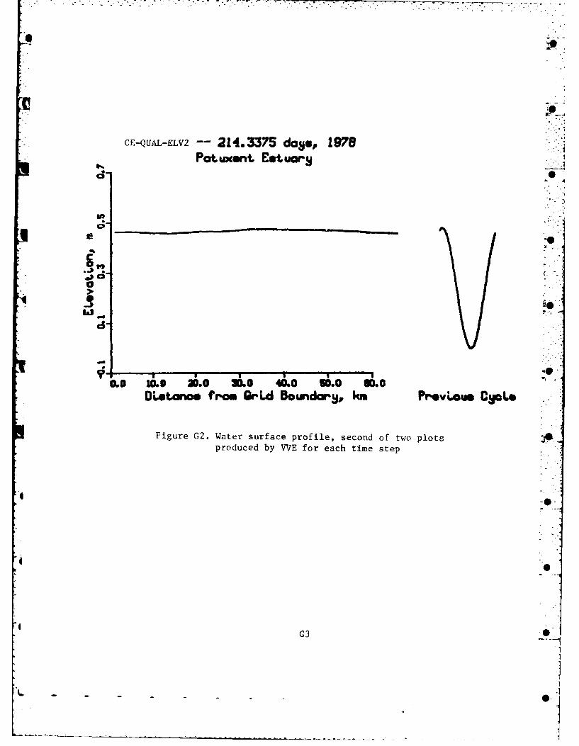
CE-QUAL-ELV2 -- 214.3375 dapj, 1978Pot wcent. Eat uary

0d -

In

0;

* ~G3

La

J |. - . -. • -. * . - _t

APPENDIX H: JULIAN DATE CALENDAR

Day Jon Fel; Ma, Ap' May June July Aug Sep Oct Nov Dec Day

1 001 032 060 091 121 152 182 213 244 274 305 335 I

2 002 033 061 092 122 153 183 214 245 275 306 336 2

3 003 034 062 093 123 154 184 215 246 276 307 337 3.

4 004 035 063 094 124 155 185 216 247 27; 308 338 4

5 005 036 064 095 125 156 186 217 248 278 309 339 5

6 006 037 065 096 126 157 187 218 249 279 310 340 6

7 007 038 066 097 127] 150 188 219 250 280 311 341 7

8 008 039 067 098 128 159 189 220 251 181 312 342 8

9 009 040 068 099 129 160 190 221 252 282 313 343 9

10 010 041 069 100 130 161 191 222 253 283 314 344 10

II Oil 042 070 101 131 162 192 223 254 284 315 345 I"

12 012 043 071 102 132 163 193 224 255 285 316 346 12

13 013 044 072 103 133 164 194 225 256 286 317 347 13

1 01 4l1 045 073 104 134 165 195 226 257 287 318 348 14

15 015 046 074 105 135 166 196 227 258 288 319 349 15

36 016 047 075 106 136 167 197 228 259 289 320 350 16"

17 017 048 076 107 137 168 198 229 260 290 32; 351 37,

18 018 9 i 077 108 138 169 199 230 261 29 122 352 38

#9 019 050 078 109 139 170 200 231 262 292 323 353 19

20 020 051, 079 330 340 17k 203 232 263 293 324 354 20

21 02, 052 080 111 141 172 202 233 264 294 325 355 23

222 2 2 053 081 112 142 173 203 234 265 295 326 3/ "

56 2 :2-

23 023 054 I 082 13 143 174 204 235 266 296 327 357 23

24 024 05, 083 114 144 175 205 236 267 297 32b 358 24

25 025 056 084 115 145 176 206 237 26 298 329 359 25

26 026 057 085 116 146 177 207 238 269 299 330 360 26

27 027 058 086 117 147 178 208 239 270 300 331 361 27

28 028 059 087 118 148 179 209 240 271 301 332 362 28

29 _029 _ 088 119 149 180 210 241. 272 302 333 363 29

30 030 089 20 10 31 ,1 242 273 303 334 364 30

31 031 090 151 212 24J 304 365 31

H1-I

.e.

* -------.- * .--.... m

In accordance with letter from DAEN-RDC, DAEN-ASI dated22 July 1977, Subject: Facsimile Catalog Cards forLaboratory Technical Publications, a facsimile catalogcard in Library of Congress MARC format is reproducedbelow.

Buchak, Edward M.User guide for CE-QUAL-ELV2 : A longitudinal-vertical,

time-varying estuarine water quality model / by EdwardM. Buchak, John Eric Edinger (J.E. Edinger Associates,Inc., Wayne, Pennsylvania). -- Vicksburg, Miss. :.U.S.Army Engineer Waterways Experiment Station ; Springfield,Va. : available from NTIS, 1982.

101 p. in various pagings ; ill. ; 27 cm. --(Instruction report ; EL-82-1)Cover title."December 1982."Final report."Prepared for Office, Chief of Engineers, U.S. Army

under Purchase Order No. DACW39-81-M-2788.""Monitored by Environmental Laboratory, U.S. Army

Engineer Waterways Experiment Station."Bibliography: p. 57-58.

Buchak, Edward M.User guide for CE-QUAL-ELV2 : A longitudinal : ... 1982.

(Card 2)

1. CE-QUAL-ELV2 (Computer program). 2. Computerprograms. 3. Estuarine ecology. 4. Patuxent RiverEstuary (Md.) 5. Water quality. I. Edinger, JohnEric. II. United States. Army. Corps of Engineers.Office of the Chief of Engineers. III. U.S. ArmyEngineer Waterways Experiment Station. EnvironmentalLaboratory. IV. Title V. Series: Instructionreport (U.S. Army Engineer Waterways Experiment Station)EL-82-1.TA7.W34i no.EL-82-1

0

0