Estimation and Short Range Forecasting of County

Level Vehicle Miles of Travel and Motor Fuel Use for

the United States (through 2015)

DRAFT

March 26, 2009

Prepared by

Frank Southworth

Tim Reuscher

Pat Hu

Center for Transportation Analysis

Oak Ridge National Laboratory

P.O. Box 2008

Oak Ridge, TN 37831

Managed By UT-Battelle, LLC

for the

U. S. Department Of Energy Under Contract No. DE-AC05-00OR22725

1

1. Introduction

This paper describes the development of a set of U.S. county-based vehicle miles of

travel and motor fuel use estimates and forecasts. The forecasts are short range, annual

forecasts out to year 2015. A range of forecasts can be generated based on different

assumptions associated with household travel growth and alternative fuel use scenarios.

The principal objective of the work is to produce a set of fuel demand forecasts that can

support both the analysis of regional fuel use trends as well as provide information useful

to the design of future alternative fuel supply infrastructures, including studies of the best

way to sequence the connection of alternative fuel resource sites to emerging consumer-

driven fuel markets. The present study is focused on private vehicle (automobile,

motorcycle) household travel. The forecasts make use of a variety of econometric

modeling steps and integrate data from a number of different government datasets. An

important requirement of the forecasts was that they remain consistent with the

information contained in these datasets, reflecting the latest government estimates and

predictions concerning historical and anticipated household travel activity levels, as well

as expected trends in motor vehicle efficiencies (i.e. in average on the road miles per

gallon statistics). A range of fuel use forecasts are reported, reflecting the uncertainty in

some of the parameters used while also demonstrating the impacts of specific

assumptions.

The paper proceeds by describing each of the major computation steps in the fuel

forecasting process in the sequence they were developed, and detailing the data sources

used in each case. The process is very much a data driven one that tries to make as much

use as possible of existing data sources. The available data, while rich in a number of

attributes, are limited in their ability to provide statistically robust coverage at the level of

spatial disaggregation required for the entire nation. As a result, a number of statistical

models are used to create both a base case set of vehicle miles of travel and fuel use

estimates as well as project these estimates into the short-term future. A high level flow

chart of the entire forecasting process is shown in Figure 1. The figure lists the principal

data sources used at each step in what can be viewed as a four step process: 1) estimate

2

annual household VMT at the county level; 2) forecast this VMT into the future; 3)

estimate household fuel consumption by fuel type for the latest year for which sufficient

data is available (currently selected to be 2006); and 4) using the latest national fuel use

forecasts, project this fuel use into the future and distribute it across states and counties

using the county VMT forecasts derived from steps 1 and 2.

Census 2000 County-Based Household Population

Estimates

NHTS-Based Tract/County VMT Estimates

Percentage Change in Fuel Shares 2006 to 2015 (EIA

AEO09) Gasoline Diesel, Ethanol (Gasohol, E85), Other

Alternative Fuels

FHWA and EIA Light Duty Vehicle Annual VMT

Estimates by State, Vehicle Types and Fuel Types

FHWA Highway Statistics and EIA AFV State Fuel

Use Percentages by Fuel Type

1. Create County-Based

Household VMT Estimates

3. Estimate 2006 Household

Fuel Use by County and

Fuel Type

4. Forecast Year (2015)

Fuel Use Trends by

County and Fuel Type

Principal Data Sources

FHWA (Highway Statistics) and EIA (AEO09)

Annualized Average VMT Growth Rates 2001-

2006

Census Bureau 2015 County-Based Household

Population Forecasts

Principal Computational Steps

2. Generate County-Based

VMT Forecasts

Figure 1. Principal Steps and Data Sources Used to Produce County Level VMT

and Fuel Use Forecasts

2. Base Year Household VMT Estimation

Vehicle miles of travel (VMT) measures were generated using the National Household

Travel Survey (NHTS) “Transferability” process and its associated Census tract-level

database.1 This process, which is now available online to users, is described in detail by

1 Accessible for online use at http://nhts-gis.ornl.gov/transferability/

3

Hu et al (2007). In summary here, a household‟s major socio-economic and geographic

travel determinants are first quantified. A multi-step process involving a combination of

cluster analysis and regression analysis is used to assign trip purpose-specific daily trip

rates and daily VMT estimates to specific Census tracts based on the number and types of

households contained within each Tract. In doing so a wide range of explanatory factors

were considered, including household income and buying power, vehicle ownership,

stage in household life cycle, metropolitan area size class, population density, cost of

living, cost of transportation, region of the country, number of workers who use public

transit, and number of bus and train routes within the Census tract. For the 2001 NHTS

database the Transferability software translates these results into tract level daily person

trips and daily VMT cross-classified by five trip purposes (Home based Work, Home

base Shopping, Home Based Social/Recreational, Other Home based and Non-Home

based trips), five household size classes (,1,2,3, 4 and 5+ persons per household), and five

vehicle ownership classes (0,1,2,3,4 + vehicles per household). County level VMT

estimates can then be obtained by summing over the VMT for all tracts within a county.

Annual household VMT totals by tract are derived by multiplying the resulting VMT

rates per household class by household population expansion factors from the 2000

Census, and by multiplying the resulting number of daily trips by 365. These tract based

estimates are then summed into their respective counties. Growth of these county VMT

figures to 2006, the base year from which fuel consumption estimates are created, is

described below.

3. Household VMT Forecasts

The above described county household VMT estimates for year 2000 are used as a base

from which to project household VMT into future years. This is done by combining data

on the growth in VMT per household over time with the growth (or decline) in travel due

to projected increases (or decreases) in U.S. household populations. Currently, the VMT

growth trend is based on nationally averaged VMT growth statistics, while the growth in

population is derived at the county level.

4

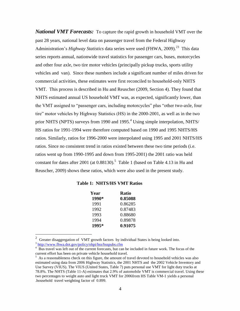
National VMT Forecasts: To capture the rapid growth in household VMT over the

past 28 years, national level data on passenger travel from the Federal Highway

Administration‟s Highway Statistics data series were used (FHWA, 2009).23

This data

series reports annual, nationwide travel statistics for passenger cars, buses, motorcycles

and other four axle, two tire motor vehicles (principally pickup trucks, sports utility

vehicles and van). Since these numbers include a significant number of miles driven for

commercial activities, these estimates were first reconciled to household-only NHTS

VMT. This process is described in Hu and Reuscher (2009, Section 4). They found that

NHTS estimated annual US household VMT was, as expected, significantly lower, than

the VMT assigned to “passenger cars, including motorcycles” plus “other two-axle, four

tire” motor vehicles by Highway Statistics (HS) in the 2000-2001, as well as in the two

prior NHTS (NPTS) surveys from 1990 and 1995.4 Using simple interpolation, NHTS/

HS ratios for 1991-1994 were therefore computed based on 1990 and 1995 NHTS/HS

ratios. Similarly, ratios for 1996-2000 were interpolated using 1995 and 2001 NHTS/HS

ratios. Since no consistent trend in ratios existed between these two time periods (i.e.

ratios went up from 1990-1995 and down from 1995-2001) the 2001 ratio was held

constant for dates after 2001 (at 0.88130).5 Table 1 (based on Table 4.13 in Hu and

Reuscher, 2009) shows these ratios, which were also used in the present study.

Table 1: NHTS/HS VMT Ratios

Year Ratio

1990* 0.85088

1991 0.86285

1992 0.87483

1993 0.88680

1994 0.89878

1995* 0.91075

2 Greater disaggregation of VMT growth factors by individual States is being looked into.

3 http://www.fhwa.dot.gov/policy/ohpi/hss/hsspubs.cfm

4 Bus travel was left out of the current forecasts, but can be included in future work. The focus of the

current effort has been on private vehicle household travel. 5 As a reasonableness check on this figure, the amount of travel devoted to household vehicles was also

estimated using data from 2006 Highway Statistics, the 2001 NHTS and the 2002 Vehicle Inventory and

Use Survey (VIUS). The VIUS (United States, Table 7) puts personal use VMT for light duty trucks at

78.8%. The NHTS (Table 11-A) estimates that 2.9% of automobile VMT is commercial travel. Using these

two percentages to weight auto and light truck VMT for 2006from HS Table VM-1 yields a personal

.household travel weighting factor of 0.899.

5

1996 0.90584

1997 0.90093

1998 0.89603

1999 0.89112

2000 0.88621

2001* 0.88130

2002 0.88130

2003 0.88130

2004 0.88130

2005 0.88130

2006 0.88130 * Highlighted years were survey years for the National Personal Transportation (NPTS)

and its successor the National Household Travel Survey (NHTS).

After this adjustment, simple linear regression, arithmetic moving average (ARIMA), and

a weighted average of the regression-ARIMA models were fitted to annual VMT data

covering the period 1980 to 2006. The steady rise in annual household VMT over this

period (see Figure 2) means that each of these methods fits the historic data closely.

0

500000

1000000

1500000

2000000

2500000

3000000

3500000

4000000

1980

1982

1984

1986

1988

1990

1992

1994

1996

1998

2000

2002

2004

2006

2008

2010

2012

2014

PREDICTED VMT (Millions of Miles)

Highway Statsitics VMT (Millions of Miles)

Figure 2. National Passenger VMT Forecast based on Linear Regression.

6

Of concern, however, is the effect, and potential for sustainability, of the rapid drop in

VMT nationwide post-20066, and not reflected in the above figure, as well as the recently

described decline in the annualized rate of VMT growth since 2004 (see Puentes and

Tomer, 2008).

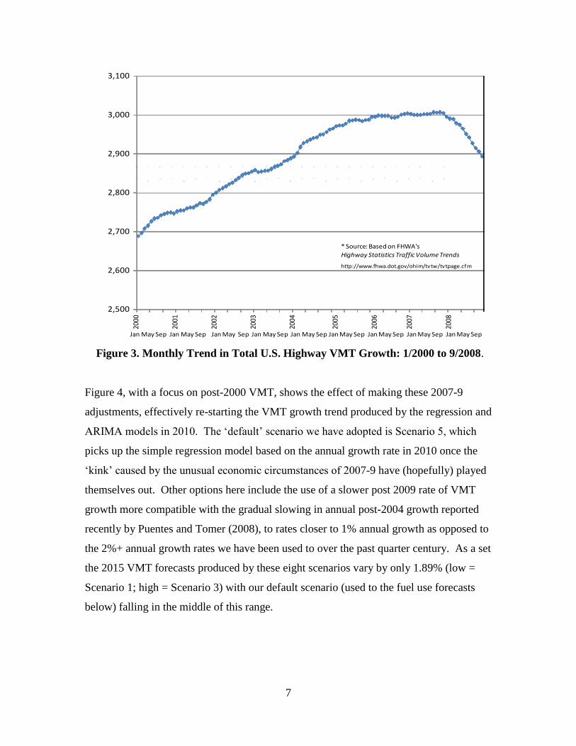
Figure 3 shows this very recent and unprecedented national trend in total (auto plus truck)

VMT. With such considerations in mind eight different VMT forecasts based on the

FHWA data were produced. These forecasts were then compared with two scenarios

based on the latest annual VMT forecasts by the Energy Information Administration

(EIA, 2009a, Table 50). This produced the following eight short range VMT projections,

termed here VMT scenarios:

Scenario 1: Use EIA growth rates for 2008 starting at 2010

Scenario 2: Pick up Simple Regression (SR) 2006 growth rates at 2010

Scenario 3: Pick up ARIMA 2006 growth rates at 2010

Scenario 4: Pick up a weighted average of SR and ARIMA2006 growth rates at 2010

Scenario 5: Pick up SR 2010 growth rates at 2010

Scenario 6: Pick up ARIMA 2010 growth rates at 2010

Scenario 7: Pick up weighted average of SR and ARIMA 2010 growth rates at 2010

Scenario 8: Pick up EIA 2010 growth rates at 2010

where growth rates refer here to the annual growth in light duty vehicle VMT forecasts

contained in the Energy Information Administration‟s (EIA‟s) most recent annual Energy

Outlook for 2009 (EAI, 2009a). Each of these scenarios represents a 2010 to 2015

growth rate projection preceded by a short term adjustment to the 2007 and 2008 VMT

estimates reported by FHWA‟s Highway Statistics series. This is done in order to capture

the noticeable downward trend in household VMT observed during 2007 and 2008 and

its anticipated continuation for at least some portion of 2009.

6 See http://www.fhwa.dot.gov/ohim/tvtw/tvtpage.cfm

7

2,500

2,600

2,700

2,800

2,900

3,000

3,100

* Source: Based on FHWA's

Highway Statistics Traffic Volume Trends

http://www.fhwa.dot.gov/ohim/tvtw/tvtpage.cfm

2000

2001

2002

2003

2004

2005

2006

2007

2008

Jan May Sep Jan May Sep Jan May Sep Jan May Sep Jan May Sep Jan May Sep Jan May Sep Jan May Sep Jan May Sep

Figure 3. Monthly Trend in Total U.S. Highway VMT Growth: 1/2000 to 9/2008.

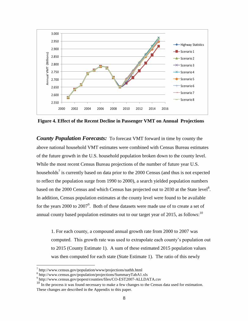
Figure 4, with a focus on post-2000 VMT, shows the effect of making these 2007-9

adjustments, effectively re-starting the VMT growth trend produced by the regression and

ARIMA models in 2010. The „default‟ scenario we have adopted is Scenario 5, which

picks up the simple regression model based on the annual growth rate in 2010 once the

„kink‟ caused by the unusual economic circumstances of 2007-9 have (hopefully) played

themselves out. Other options here include the use of a slower post 2009 rate of VMT

growth more compatible with the gradual slowing in annual post-2004 growth reported

recently by Puentes and Tomer (2008), to rates closer to 1% annual growth as opposed to

the 2%+ annual growth rates we have been used to over the past quarter century. As a set

the 2015 VMT forecasts produced by these eight scenarios vary by only 1.89% (low =

Scenario 1; high = Scenario 3) with our default scenario (used to the fuel use forecasts

below) falling in the middle of this range.

Jan - 00

May - 00

Sep - 00

Jan - 01

May - 01

Sep - 01

Jan - 02

May - 02

Sep - 02

Jan - 03

May - 03

Sep - 03

Jan - 04

May - 04

Sep - 04

Jan - 05

May - 05

Sep - 05

Jan - 06

May - 06

Sep - 06

Jan - 07

May - 07

Sep - 07

Jan - 08

May - 08

Sep - 08

8

2.550

2.600

2.650

2.700

2.750

2.800

2.850

2.900

2.950

3.000

2000 2002 2004 2006 2008 2010 2012 2014 2016

An

nu

al

VM

T (

Bil

lio

ns)

Highway Statistics

Scenario 1

Scenario 2

Scenario 3

Scenario 4

Scenario 5

Scenario 6

Scenario 7

Scenario 8

Figure 4. Effect of the Recent Decline in Passenger VMT on Annual Projections

County Population Forecasts: To forecast VMT forward in time by county the

above national household VMT estimates were combined with Census Bureau estimates

of the future growth in the U.S. household population broken down to the county level.

While the most recent Census Bureau projections of the number of future year U.S.

households7 is currently based on data prior to the 2000 Census (and thus is not expected

to reflect the population surge from 1990 to 2000), a search yielded population numbers

based on the 2000 Census and which Census has projected out to 2030 at the State level8.

In addition, Census population estimates at the county level were found to be available

for the years 2000 to 20079. Both of these datasets were made use of to create a set of

annual county based population estimates out to our target year of 2015, as follows:10

1. For each county, a compound annual growth rate from 2000 to 2007 was

computed. This growth rate was used to extrapolate each county‟s population out

to 2015 (County Estimate 1). A sum of these estimated 2015 population values

was then computed for each state (State Estimate 1). The ratio of this newly

7 http://www.census.gov/population/www/projections/nathh.html

8 http://www.census.gov/population/projections/SummaryTabA1.xls

9 http://www.census.gov/popest/counties/files/CO-EST2007-ALLDATA.csv

10 In the process it was found necessary to make a few changes to the Census data used for estimation.

These changes are described in the Appendix to this paper.

9

computed sum to the Census 2015 total state population estimates was then

calculated. This ratio was then multiplied by the estimate of county population

created earlier (County Estimate 1) to make the county estimates consistent with

the state estimates (County and State Estimates 2).

2. Since the NHTS Transferability data is also based on the 2000 Census data, a

bridge must be constructed between the final 2015 county population estimates

and 2000 Census estimates. For simplicity‟s sake, for each county a simple ratio

of the 2015 estimate to 2000 Census value was calculated. This ratio was then

applied to each Census Tract‟s household count to grow the 2000 data into 2015

estimates.

Note that in the current estimates we have ignored the difference between population and

household counts. Current Population Survey numbers11

show 2.58 persons per

household in 2001. This remained the same until 2003, when the number declined

marginally to 2.57. This number stayed the same through 2006, until finally dropping to

2.56 in 2007, the most recent year for which data was available. Given this extremely

slow level of decline, combined with the difficulty in determining the changes in the

household size distribution, which would be needed in developing population numbers

for use with the Transferability data, no change in average household size is assumed

through 2015. Given this, the adjustment from 2000 to 2015 households is simply the

same adjustment made to the population numbers – 2000 households multiplied by the

ratio of 2015 Population Estimates/2000 Census Population numbers. For forecasting

further into the future it is then a simple process to introduce any gradual change in the

number of persons per household into the forecast.

Combining VMT Estimates and Population Forecasts: The next step in the

process combines the above results. First the 2001 NHTS-based household VMT rates for

each tract are multiplied by the number of households forecast to be in each county and

state, in each future year up to year 2015. Summing over all household groups, trip

11

http://www.census.gov/population/www/socdemo/hh-fam.html

10

purposes and tracts within a given county produces an aggregate county-based VMT

forecast for each year, based solely on Census determined population growth. These

VMT figures are then reconciled with the annual, nationwide VMT estimates and

projections derived from the regression and ARIMA modeling of the FHWA and EIA

datasets described above. The resulting forecasts are therefore compatible with the most

recently available data on:

o the way in which VMT varies across household socio-economic groups and trip

purposes, as described in the 2001 NHTS,

o the growth in Census Bureau projected county and state population totals, and

o both longer term and more recent nationwide growth trends, compatible with

the latest FHWA or EIA data sources.12

4. Year 2006 State and County Fuel Consumption by Fuel Type

VMT forecasts are turned into fuel use forecasts starting with a year 2006 base. This was

the latest year for which fuel consumption data by individual states was available. The

following two step process was followed, with a number of detailed adjustments to

ensure compatibility of data sources being required along the way, as explained below:

1. Use FHWA, EIA and census Bureau data sources to put state- based estimates

of gallons of fuel used for highway travel in 2006 into their gasoline-gallon

equivalents (GGEs)

2. Distribute this fuel consumption by state and fuel types across the counties

within a state on the basis of their share of that state‟s private vehicle household

travel (VMT).

12

Building on this framework, additional VMT forecasts can also be generated by further disaggregating

the VMT growth trends reported in FHWA‟s Highway Statistics dataset. This can be done by developing

separate VMT projections by State or by a broader regional partitioning of the nation as suggested by

further statistical analysis, and thereby adding additional geographic information to the step by step

proportional fitting process described here..

11

3. Replace each state‟s ethanol allocations to E-85 flex-fuel vehicles with an

alternative county allocation based on a detailed geographic analysis of the

location of existing E-85 refueling stations.

State Fuel Consumption Totals by Fuel Type: Fuel use data was available at the

state level from two sources: the annual estimate of gasoline and “special” fuels

consumed in each state from FHWA‟s Highway Statistics series (HS Table MF 21), and

the EIA‟s estimates of alternative fuels (Compressed Natural Gas, Electric, Hydrogen,

Liquid Natural Gas, Liquid Petroleum Gas Ethanol E-85, and Other Fuels) consumption

(EIA, 2009b).13

Since the gasoline consumption figures from Highway Statistics included

gasohol, a third source of data required was the percentage of ethanol used in this

gasoline. The latest readily available data on this at the state level is also reported in

Highway Statistics (Table MF33e), but only for as recently as 2004, which became the

default set of values for the present study. In combining these various data sources all

fuel was converted to its gasoline-gallon equivalent (GGE).

With diesel being used mostly in trucks, a household travel diesel use factor was also

needed. This was estimated using the data reported in the Edition 27 of Transportation

Energy Data Book (Davis et al, 2008: Table 2.5) in which diesel consumption on

highways (in million Btu) is broken down into automobile (“cars”), light duty truck, bus,

and heavy duty truck use. After subtracting heavy truck use, this left a proportion of light

truck use to be removed. Data from the 2002 Census Bureau‟s Vehicle Inventory and Use

Survey (VIUS: Census Bureau, 2006) was used for this purpose. According to the VIUS

some 81.5% of light truck use is for personal travel. Subtracting the remaining 18.5% of

the energy used in light duty trucks yielded an estimated 2.1% of total automobile plus

light truck energy use for household travel being assigned to diesel in 2006 (=

approximately 6.3% of fuel used in 2006 for all automobile and motorcycle on-highway

travel being assigned to diesel).

13

Source: Energy Information Administration, Office of Coal, Nuclear, Electric, and Alternate Fuels.

http://www.eia.doe.gov/fuelrenewable.html

http://www.eia.doe.gov/cneaf/alternate/page/atftables/afvtransfuel_II.html#consumption

12

Finally, since EIA‟s 2006 alternative fuels data ( given in GGEs) does not separate out

household from other (i.e. commercial) travel consumption, these figures were reduced

by the (NHTS/HS) VMT adjustment ratio of 0.88310 described above for computing

household only travel.

The result of these various computations and adjustments is a set of state specific private

motor vehicle fuel use totals for 2006 converted to GGEs; one that is consistent with

FHWA and EIA reporting of data at the state level.

County Fuel Use Estimates for 2006: These state fuel use totals are then

distributed across the counties within each state on the basis of that county‟s share of its

state‟s household estimated household VMT in 2006. Using the mid-range Scenario 5

household VMT numbers (cf. Section 3) produced a 50 state plus Washington DC, VMT

weighted average miles per gallon (mpg) estimate of 20.68. This figure is just slightly

above the nationwide mpg estimate reported in EIA latest Annual Energy Outlook (EIA,

2009a, Table 69) of 20.37 mpg. State average 2006 mpg‟s from this exercise range from

15.6 mpg for Louisiana up to 24.8 mpg for Idaho.

E-85 Fuel Use in U.S. Counties in 2006:

Given the growing interest in ethanol fueled vehicles and (see section 5) their anticipated

increase in use by 2015 the state specific totals for E-85 consumption in 2006 reported by

EIA were assigned to counties on the basis of the number of publicly available E-85

refueling stations in that county. Given the importance of proximity to a refueling station

in the selection of this fuel (see Greene, 1998, 2001) this offers a much better method of

distributing the fuel demand than a simple county-based VMT weighting. Just how to

allocate the amount of ethanol obtained from each refueling station is more problematic.

Two options were tested: 1) locate each refueling station according to its 5-digit zip code,

and use that zip code area‟s population to weight its allocation of the state‟s reported E-

85 use in 2006, then assign each zip code areas fuel use to its appropriate county; and 2)

allocate the E-85 on the basis of number of stations per county. Option 2 results were

13

used here as the default. The data for this exercise was obtained from the station

addresses listed by state on the U.S. Department of Energy‟s (DOE) Office Energy

Efficiency and Renewables Alternative Fuels and Advanced Data center website

(EERE,2009). 14

Figure 5 shows the heavy concentration in the Midwest of publicly available as well a

planned E-85 refueling stations, as reported on this website (March 2009).

Figure 5. Counties with Public and/or Planned Ethanol (E-85) Refueling Stations

(As of March, 2009)

5. Year 2015 County Fuel Use Forecasts by Fuel Type

The final step in the process illustrated in Figure 1 is to project the 2006 county fuel use

forecasts into future years, and specifically out to year 2015. This meant accounting for

both household VMT growth (or in some counties, decline) as well as the changes in

14

http://www.afdc.energy.gov/afdc/stations/advanced.php

14

vehicle fuel efficiency (average mpg) between the two years. This was done in the

following steps:

1. Compute the state VMT estimates for 2015 by summing the forecast VMT

over all counties in the state.

2. Compute the estimated average mpg for each state in 2015 by multiplying the

2006 averaged state mpg by the % change in average nationwide mpg by 2015 as

reported in EIA‟s Annual Energy Outlook for 2009 (early release: EIA, 2009a).

3. Compute the 2015 total GGEs per state by dividing the 2015 state VMT by its

average mpg from step 2.

4. Project the 2006 fuel consumption shares (in GGEs) onto these 2015 state

GGE totals.

5. Adjust these fuel shares to match the shift in each share predicted by the EIA‟s

Annual Energy Outlook (EIA, 2009a, Table 46).15

In doing so adjust the E-85 fuel

shares to reflect the distribution of planned as well as publicly available E-85

refueling stations.16

7. Distribute the resulting state fuel totals to counties on the basis of each

county‟s share of its 2015 state VMT.

In this manner it is possible to capture some of the effects of different state geographies

on mpg efficiencies and hence on total fuel consumption. The resulting 2006 and 2015

nationwide fuel shares are shown in Table 2.

Table 2: Aggregate Fuel Shares (in % GGEs) 2006 and 2015

Gasoline Diesel

Ethanol

from

Gasohol

Ethanol

from E-85

Other

Alternative

Fuels Total

2006 95.89 2.05 1.79 0.03 0.25

2015 93.51 2.38 1.73 2.14 0.24

15

Note that the shifts in fuel shares between 2006 and 2015 are used, rather than the 2015 fuels share totals

directly. This is done to allow for slightly different base fuel shares caused by computing shares for

household private vehicle travel only. 16

Planned as well as existing public E-85 re-fuelling stations are listed by state on the DOE/EERE

website at http://www.afdc.energy.gov/afdc/stations/advanced.php

15

These shifts reflect EIA‟s anticipated increase in the use of E-85 flex-fuel ethanol

vehicles over the next few years in response to recent federal legislation encouraging this

trend. The 2015 VMT weighted average mpg from these calculations comes in at 23.06

mpg for the 50 state plus Washington DC, while individual state average mpg‟s for 2015

range from 17.6 mpg for Louisiana up to 27.6 mpg for West Virginia. This reflects an

11.3% increase in private vehicle household mpg for the 50 states plus Washington DC

dataset. This increased efficiency offsets an estimated 5.87 % increase in overall

household VMT for the 50 states plus Washington DC to produce an estimated reduction

in motor fuel energy use for private vehicle household travel of 4.9% by 2015.

6. Example Output and GIS Mapping

To allow visual analysis, county based VMT and fuel consumption results have been

attached to a set of county latitudes and longitudes. These data are easily exported to a

geographic information system (GIS) software. Figure 6 maps the estimated % change in

each county‟s household private vehicle VMT from 2006 to 2015, showing the decline in

total VMT in many rural counties and especially in a north-south band of counties

running down the center of the nation from North Dakota to Texas.

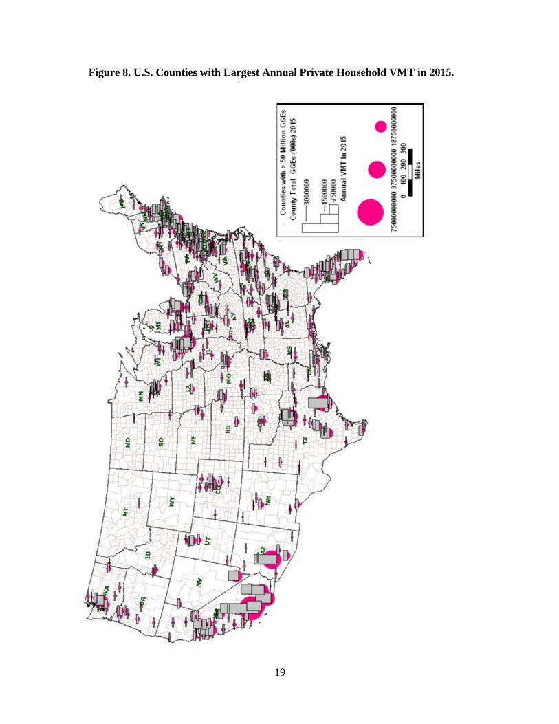
Figures 7, 8 and 9 map some of the fuel consumption results, for clarity of presentation

here showing only those counties estimated to consume at least 50 million total gallons of

motor fuel annually in 2015 (i.e. counties with at least some 75,000 in use vehicles). All

of these mappings also the default (scenario 5) VMT annual growth scenario discussed

above, combined with the estimated change in alternative fuel shares (and notably the

growth in ethanol use) from EIA‟s Annual Energy Outlook 2009 (early release) forecast.

Figure 7 maps the U.S. counties with the largest estimated total GGEs consumed in 2006,

summed over all fuel types (represented by the height of the grey bars) as well as the

projected percentage increase in total GGEs between 2006 and 2015 (represented by the

size of the red circles). Figure 8 maps the estimated county GGE totals in 2015, again

summed over all fuel types (represented by the height of the grey bars), along with the

estimated annual county VMT in 2015 (represented by the size of the red circles). Figure

16

9 shows the estimated shares of alternative to gasoline fuels (diesel, ethanol from

gasohol, ethanol in E-85 vehicles, and “other” fuels), again highlighting U.S. counties

with over 50 million total estimated GGEs (including gasoline) in 2015. The size of each

pie chart here is proportional to each county‟s estimated alternative, non-gasoline, fuel

demand in 2015. Significant regional differences in alternative fuel shares are evident

from this mapping, which assumes the concentrations of E-85 growth in those counties

already supporting this fuel type described above. Other scenarios, under other E-85

penetration and growth assumptions, can now also be simulated using this spreadsheet

modeling and mapping software. Longer range forecasts can also be generated using the

current scenario-based approach, using EIA and /or other forecasts for alternative fuel

penetration rates out to 2030, or by tying the VMT and associated population growth

forecasts to more elaborately developed alternative fuel adoption models.

17

Figure 6. Estimated Percentage Change in Household Private Vehicle VMT by U.S.

County from 2006 to 2015

18

Figure 7. U.S. Counties with the Most GGE’s Consumed in 2006

19

Figure 8. U.S. Counties with Largest Annual Private Household VMT in 2015.

20

Figure 9. Alternative Fuel Shares in 2015: Counties with Over 5 GGEs

21

References

Census Bureau (2006) Vehicle Inventory and Use Survey. 2002 Data Releases. Census

Bureau,, U.S. Department of Commerce, Washington D.C.

http://www.census.gov/svsd/www/vius/2002.html

Davis, S.C, Diegel, S.W. and Boundy, R.G. (2008) Transportation Energy Data Book.

Edition 27. Oak Ridge National Laboratory. Oak Ridge, TN 37831. ORNL-6981.

http://cta.ornl.gov/data/download27.shtml

EERE (2009) Alternative Fuels and Advanced Data Center Website. Office of Energy

Efficiency and Renewables Energy. U.S. Department of Energy, Washington, D.C.

http://www.afdc.energy.gov/afdc/stations/advanced.php

EIA (2009a) Annual Energy Outlook 2009 (Early Release). Supplementary Tables.

Transportation Demand Sector. Energy Information Administration, U.S. Department of

Energy,Washington, D.C. http://www.eia.doe.gov/oiaf/aeo/supplement/index.html

EIA (2009b) Office of Coal, Nuclear, Electric, and Alternate Fuels. Energy Information

Administration, U.S. Department of Energy, Washington,

D.C.http://www.eia.doe.gov/fuelrenewable.html

FHWA (2009) Highway Statistics. Office of Highway Policy Information. Federal

Highway Administration, U.S. Department of Transportation, Washington, D.C.

http://www.fhwa.dot.gov/policy/ohpi/hss/index.cfm

Greene, D.L. (1998). “Fuel Availability and Alternative Fuel Vehicles,” Energy Studies

Review, Vol.8. 3: 215-231.

Greene, D.L. (2001). TAFV Alternative Fuels and Vehicles Choice Model

Documentation. Oak Ridge National Laboratory ORNL//TM––2001//134, Oak Ridge,

TN 37831.

Hu, P., Reuscher, T., Schmoyer, R. and Chin, S-M (2007) Transferring 2001 National

Household Travel Survey

http://nhts-gis.ornl.gov/transferability/TransferabilityReport.pdf .

Hu, P, and Reuscher, T, (2009) NHTS/NPTS Annualization. DRAFT.

Puentes, R. and Tomer, A. (2008) The Road…Less Traveled: An Analysis of Vehicle

Miles Traveled Trends in the U.S. Brookings Institution, Washington D.C.

22

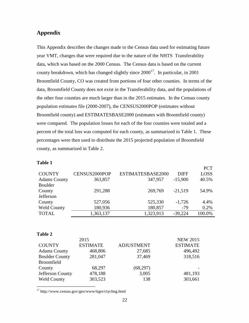
Appendix

This Appendix describes the changes made to the Census data used for estimating future

year VMT, changes that were required due to the nature of the NHTS Transferability

data, which was based on the 2000 Census. The Census data is based on the current

county breakdown, which has changed slightly since 200017

. In particular, in 2001

Broomfield County, CO was created from portions of four other counties. In terms of the

data, Broomfield County does not exist in the Transferability data, and the populations of

the other four counties are much larger than in the 2015 estimates. In the Census county

population estimates file (2000-2007), the CENSUS2000POP (estimates without

Broomfield county) and ESTIMATESBASE2000 (estimates with Broomfield county)

were compared. The population losses for each of the four counties were totaled and a

percent of the total loss was computed for each county, as summarized in Table 1. These

percentages were then used to distribute the 2015 projected population of Broomfield

county, as summarized in Table 2.

Table 1

COUNTY CENSUS2000POP ESTIMATESBASE2000

DIFF

PCT

LOSS

Adams County 363,857 347,957 -15,900 40.5%

Boulder

County 291,288 269,769 -21,519 54.9%

Jefferson

County 527,056 525,330 -1,726 4.4%

Weld County 180,936 180,857 -79 0.2%

TOTAL 1,363,137 1,323,913 -39,224 100.0%

Table 2

COUNTY

2015

ESTIMATE

ADJUSTMENT

NEW 2015

ESTIMATE

Adams County 468,806 27,685 496,492

Boulder County 281,047 37,469 318,516

Broomfield

County 68,297 (68,297) -

Jefferson County 478,188 3,005 481,193

Weld County 303,523 138 303,661

17

http://www.census.gov/geo/www/tiger/ctychng.html

23

1,599,862 0 1,599,862

Also in 2001, the independent city of Clifton Forge, VA was added to Alleghany County.

This presents the reverse problem to the Broomfield county exercise. Here, the solution

is much simpler. The combined Census 2000 population of Clifton Forge and Alleghany

County was computed, with percentage shares of for each, 24.91% and 75.09%,

respectively, also computed. The 2015 estimate was then simply distributed according to

these shares.

24