
Rail Demand Forecasting Estimation - gov.uk · PDF file6 Rail Demand Forecasting Estimation...
158
Rail Demand Forecasting Estimation Final Report Final Draft, Redacted Prepared for Department for Transport November 2016
Transcript of Rail Demand Forecasting Estimation - gov.uk · PDF file6 Rail Demand Forecasting Estimation...

Rail Demand Forecasting Estimation
Final Report
Final Draft, Redacted
Prepared for Department for Transport
November 2016

2 Rail Demand Forecasting Estimation
Table of Contents
1 INTRODUCTION ..................................................................................................... 4
1.1 Purpose of Rail Demand Forecasting Study ............................................................ 4
1.2 Project Approach ................................................................................................... 11
1.3 Phase 2 Modelling Approach ................................................................................. 12
2 NTS MODELLING ................................................................................................. 14
2.1 NTS Models and Results ....................................................................................... 14
2.2 Socio-economic characteristics of rail users .......................................................... 20
2.3 The impact of network effects ................................................................................ 27
2.4 Time trend effects .................................................................................................. 28
2.5 Outputs to models derived from ticket sales (RUDD models) ................................ 29
3 TICKET SALES ANALYSIS ................................................................................... 31
3.1 Introduction ........................................................................................................... 31
3.2 Scope .................................................................................................................... 32
3.3 Enhancing Rail Ticket Sales Models with NTS Trip Rate Evidence ....................... 35
3.4 General Principles of Our Modelling ...................................................................... 44
4 ESTIMATED TICKET SALES MODELS ................................................................ 52
4.1 Variables Considered ............................................................................................ 52
4.2 Long Distance London Non-Seasons .................................................................... 61
4.3 Long Distance Non-London Non-Seasons............................................................. 64
4.4 Network Area to and from London Non-Seasons................................................... 67
4.5 Network Area to London Seasons ......................................................................... 71
4.6 Non London Short, Non-Seasons .......................................................................... 75
4.7 Non London Seasons ............................................................................................ 78
5 BACKCASTING..................................................................................................... 83
5.1 Approach to Backcasting ....................................................................................... 84
5.2 Rest of Country to London (Ordinary tickets) ......................................................... 86
5.3 Network Area to/from London (Ordinary tickets) .................................................... 88
5.4 Network Area to London (Season tickets).............................................................. 91
5.5 Non-London (Season tickets) ................................................................................ 93
5.6 Non-London short distance (Ordinary tickets) ........................................................ 95
5.7 Non-London long distance (Ordinary tickets) ......................................................... 98
5.8 Summary of results ............................................................................................. 100

Final Report 3
6 CONCLUSIONS .................................................................................................. 103
6.1 Novel Analysis ..................................................................................................... 103
6.2 Application for forecasting purposes .................................................................... 106
6.3 Recommended elasticities and recommendations for forecasting ....................... 107
6.4 Recommendations for Data Collection ................................................................ 116
6.5 Recommendations for Implementing the Forecasting Framework ....................... 117
6.6 Recommendations for Further Research ............................................................. 118
ANNEX A DETAILED SPECIFICATION AND RESULTS OF THE NTS RAIL FREQUENCY
MODELS ............................................................................................................. 121
ANNEX B RUDD DATA PROCESSING ........................................................................... 135
ANNEX C TICKET TYPE AND JOURNEY PURPOSE SPLITS ....................................... 148
ANNEX D QUALITY ASSURANCE SUMMARY ............................................................... 157

4 Rail Demand Forecasting Estimation
1 Introduction and Executive Summary
1.1 Executive Summary
Background and Aims 1.1.1
This study is concerned with quantifying how variables outside of the control of the rail
industry, commonly termed external factors, impact upon the demand for rail travel. These
variables tend to be key drivers of rail demand, with employment and income recognised as
being particularly important drivers of demand in the recommendations of the railway
industry’s Passenger Demand Forecasting Handbook (PDFH).
The background to this project, and the reasons why further research on this crucial subject
is clearly warranted, is that there is broad acceptance amongst key stakeholders and
practitioners that:
Rail growth figures derived from PDFH and WebTAG recommendations have not generally been performing well in explaining recent growth in rail demand (see charts below);
Whilst the current forecasting framework covers the key demand drivers of income and employment there are other important influential variables which are currently not covered in PDFH;
Recent econometric studies, which had aimed to provide updated values for existing PDFH parameters and insights into unaccounted influences on rail demand, have not provided entirely convincing findings;
PDFH specifically under-forecasts non-London demand, particularly for commuting into core cities, a factor that has been recognised for some years.
Given this background, the objective of the study was to improve the performance of
elasticity based rail demand forecasting, to be achieved both by updated evidence on
existing parameters and, within the constraints of budget and data availability, through
enhancements to the existing PDFH forecasting framework.
We should point out that this is not the first occurrence of PDFH performing poorly in
explaining rail demand. PDFH v3, with its combination of positive GDP elasticities which
were unable to offset outdated negative time trends, could not explain the strong and
sustained demand growth in the years after privatisation. The result was that PDFH v4 in

Final Report 5
2002, inspired by the investigations of the industry funded National Passenger Demand
Forecasting Framework Study in 1999, provided both revised GDP elasticities and a
significantly enhanced framework that replaced time trends with a range of variables dealing
with inter-modal competition.
General Approach 1.1.2
The same general approach has been followed here as with the PDFH v4 update: the
provision of revised elasticities for existing parameters along with enhancements to the
forecasting framework which here largely take the form of a broader range of socio-
economic factors with an emphasis upon those for which there are forecasts.
From the outset, our intention was to use National Travel Survey (NTS) data, which we
believe to be a very much under-exploited resource as far as understanding rail demand is
concerned, not so much as a free-standing forecasting tool, which it could be, but rather as a
means of providing insights into the effects of a range of socio-economic factors on rail
demand that are not addressed in current models but which, critically, could be used to
enhance those models. Our argument is that whilst conventional rail demand models
containing, say, GVA, employment, overall population and car ownership, could in principle
be enhanced by adding a range of socio-economic variables, past experience, as evidenced
in our literature review, shows that the free estimation of such effects is generally
unsuccessful.
Our approach was therefore to conduct NTS analysis to provide parameters relating to
various socio-economic and demographic factors which can then be imported into
conventional rail demand models, based on ticket sales data, to serve as constraints on key
parameters for which free estimation would not provide credible results.
The study was split into two phases.
Phase 1, conducted over summer 2015, was largely exploratory and consisted of a number
of work-streams:
It conducted what can be regarded as the most extensive review of evidence relating to exogenous drivers of rail demand in Great Britain along with a discussion of the evolution of PDFH’s treatment of these key demand drivers.
A data capability review covering the DfT’s Rail Usage and Demand Drivers Dataset (RUDD), which covers 20,000 flows over 20 years, to determine its fitness for purpose and to identify shortcomings and gaps that might be addressed.
A review of NTS data, covering its content, trends and potential key insights.
A workshop in July 2015 which shared the findings of Phase 1 with rail industry demand forecasting experts and sought views on the causes of recent strong demand growth and research direction.
A report containing recommendations for the main quantitative stage.
Phase 2 was the main quantitative phase, commencing in Autumn 2015. Its key elements
were:
Analysis of variations in individuals’ trip making as represented within the NTS data, primarily to determine the impact on rail demand of a range of socio-economic and

6 Rail Demand Forecasting Estimation
demographic variables that are not currently covered in conventional rail demand analysis.
Synthesis of the insights obtained from the analysis of NTS data to a form that can be used to enhance conventional rail demand models.
Econometric analysis of ticket sales data using the insights obtained from the NTS analysis in conjunction with the variables included in RUDD to advance understanding of rail demand through the inclusion of a broader range of external factors.
Exploration of additional factors, as data allows, that might explain the strong demand growth in recent years.
A significant back-casting exercise to test how well our emerging model parameters could explain rail demand growth since 1996 and to inform on the selection of preferred models.
We can therefore usefully summarise the ultimate outcomes of our research in terms of the
following main contributory factors. These cover:
the discrete choice analysis of the NTS data;
the econometric analysis of rail ticket sales data;
the back-casting exercise;
application for forecasting purposes;
conclusions and recommendations.
Analysis of NTS Data 1.1.3
The use of disaggregate data records for analysis has facilitated the best use of data for
examination and quantification of socio-economic drivers on rail travel. Many of these
important drivers of rail demand have not been taken into account in previous rail forecasting
models.
Below are the key findings derived from the discrete choice model analysis:
Income is a strong determinant for the choice of using rail as mode of travel. Across all purposes and geographies we observe that increasing income levels lead to an increase in the propensity to travel by rail, although increasing income levels do not seem to have such a large impact on the propensity to make multiple trips. We were not able to identify differences between income changes over time and cross-sectional income differences on rail travel.
People with full driving licences are less likely to use rail for commuting journeys and other trips. Further, as the number of cars in the household increases the propensity to travel by rail decreases. Moreover, people who have a car freely available in the household, i.e. when the number of cars in the household is equal to or exceeds the number of drivers, are less likely to make rail trips.
The presence of a company car affects the propensity for rail travel for commuting and business travel. For commute travel we observe that people in households with a company car are less likely to make rail trips. However, for business travel, the presence of a company car in the household seems to increase the likely of travelling by rail (perhaps the presence of the company car is a proxy for the type of job the person has), but decrease the likelihood of making multiple trips in a week by rail. Given the way the

Final Report 7
terms work, the trip rates for rail travel for business purposes are very similar for people with and without company cars in the household.
For commute travel, full-time and part-time workers are more likely to make rail trips than self-employed people, and full-time workers are more likely to make rail trips than part-time workers. Full-time workers are also more likely to make multiple rail commute trips than other worker types.
For business travel, part-time workers are less likely to make rail business trips than full-time or self-employed workers.
For other travel, self-employed workers and temporarily sick people, disabled people and people looking after family are less likely to make rail trips relative to full time workers; whereas, students, those who are retired, those who are unemployed and those who work part-time are more likely to make rail trips. Those who work full-time are less likely to make multiple rail trips for other purposes.
For all purposes, we observe that those working in managerial, professional or administrative occupations are more likely to travel by rail compared to those with other occupations. For other travel, we also observe that those involved in skilled trades and process, plant and machines are less likely to travel by rail.
Across purposes, we see that those who are involved in manufacturing, wholesale business, construction and health/social care sectors are less likely to travel by rail, whereas those involved in the finance sector (for commuting and other travel) and real estate (for business) are more likely to travel by rail. Moreover, for commuting, those who work in the financial sector are more likely to make multiple rail trips in the week for commuting purposes. Therefore, as the structure of the economy changes, we would expect changes in rail demand.
In general, older people and those under 16 years of age are less likely to travel by rail, whereas those who are employed and are under 25 years of age are more likely to make multiple rail commuting trips.
In general, we were not able to identify significant effects of changes in rail service variables
on rail demand from the NTS data. We suspect that this is because of the relatively coarse
geography that we could use to compare rail and NTS (local authority level). Although we did
observe for some segments that increases in access time to stations led to a decrease in the
propensity to make rail trips.
Lastly, we did observe a significant time-trend effects across most purposes and
geographies, indicating an increased likelihood of travelling by rail over time that is not
explained by socio-economic and network terms.
Estimation of Enhanced Rail Demand Models to Ticket Sales Data
The study focussed on six PDFH flow types. These were long distance London non-seasons,
long distance Non London non-seasons, Network Area to London for seasons and non-
seasons, and Non London short distance flows for seasons and non-seasons. Each of the
data sets covered annual data for the years 1995/96 through to 2013/14.
The main enhancement of the rail demand models was the inclusion of the trip rate evidence
from the analysis of the NTS data. The output of the NTS analysis was summarised in the
form of deviations from the average trip rate according to five age groups, nine occupation
types, six employment sectors and four levels of household car-availability. Data was

8 Rail Demand Forecasting Estimation
available on each of these variables for each station-to-station movement and year and
hence could be matched to the trip rate findings to determine an expected trip rate for each
movement and time period.
The expected trip rates distinguished by commuting, business and other journey purposes
and for each whether trips were based on London or not. These expected trip rates were
used to weight the population or employment term as appropriate whose parameter was
then constrained to one.
Hence the model is able to explain rail demand growth due to variations in the socio-
economic composition of the population and their different propensities to make rail trips. We
experimented with the inclusion of the NTS derived income elasticities in the trip rate index
but this invariably produced inferior results and model fit and was not retained.
The models also include what might be termed standard explanatory variables of rail fare,
generalised journey time (GJT), Gross Value Added (GVA), car fuel cost, car journey time
and, where not otherwise covered by the trip rate index, car ownership. Inclusion of a
reliability term, in the form of average minutes late (AML), did not prove successful.
The literature review of previous experience and findings strongly indicated that constraints
should be applied to the population, employment, fuel and car journey time elasticities and
indeed the importance of these was demonstrated.
Other notable developments in the reported models were:
A time trend, based on what empirical evidence exists, of a one percent reduction in GJT from 2000 to account for significant advances in digital technology and that rail travel is well placed to benefit from such developments. The annual time trend is approximately 0.99g where g is the PDFH GJT elasticity relevant to the flow. This improved model fit and forecasting performance in almost all cases.
NTS evidence was used to allow for what is widely felt to have been switching of commuters out of season tickets into ordinary tickets on London based flows.
The use of evidence from NTS to provide a firmer basis for historic car journey times.
Basing the analysis on data pooled across directions for the long distance flows where single-leg advance purchase tickets are widespread and hence directionality is unknown.
Extension of the Non London season ticket market from 20 to 50 miles.
The successful inclusion of employment within non-seasons models to reflect commuting on such tickets.
The successful inclusion of unemployment in seasons models, which might be discerning the structural changes in the employment market than many commentators believe has occurred particularly outside London.
The successful inclusion of GVA in Network Area to London seasons models.
Very large employment elasticities for flows into ‘core’ cities reflecting the structural changes in the labour market that have been ongoing for many recent years.
New and credible evidence for non-season demand in PTE areas where there is a dearth of reliable evidence.

Final Report 9
A large number of highly statistically significant and credible elasticities were obtained. Summary GVA and fare elasticities are set out in the table below. The fare elasticities tend to be very similar and generally very plausible. We report the fare elasticities here because, unlike many other explanatory variables and for reasons explained elsewhere in the document, the fare elasticities were freely estimated in all our models and the credibility of the estimates contributes to the confidence that can be placed in our findings. Nonetheless, it was the purpose of a parallel study (SYSTRA and ITS Leeds, 2016) to investigate fare elasticities in considerably more detail.
The GVA elasticities exhibit more variation, but the inclusion of the time trend in particular and to varying extents the trip rate index deflate the estimated GVA elasticity. Nonetheless, the models are better placed than current PDFH recommendations at explaining recent rail demand growth.
Flow GVA Elasticity
Fare Elasticity
Long Distance London 0.68 -0.73
Long Distance Non London Between Two Core Cities
0.97 1.24
-0.67 -0.67
Network Area to London Non Seasons Network Area from London Non Seasons
1.04 0.19
-0.69 -0.69
Non London Short Non Seasons Non London Short Non Seasons PTE
0.90 0.90
-0.87 -0.69
Network to London Seasons 0.49 -0.58
Non London Seasons Short Non London Seasons Long
-0.79 -0.20
When freely estimated, the employment elasticity for Network Area to London season tickets
turned out to be one. It was also close to one on for Non London season ticket flows
although with values a little over one for longer distance flows but in excess of two for
commuting into core cities.
Back-Casting Exercise 1.1.4
Our back-casting work reviewed emerging models and helped us select our preferred
models. It also helps us understand how the addition of different parameters has helped us
bridge gaps between the existing PDFH/WebTAG forecasting framework and actual results.
The key differences between our models and PDFH/WebTAG are typically in our different
fares elasticities – estimated using a CPI deflator over time instead of RPI – and the use of
the time trend.
For long distance travel to/from London, an unusual picture emerges. PDFH/WebTAG
overforecasts growth prior to c.2007 and underforecasts growth subsequently. Adding the
time trend to PDFH/WebTAG makes the former problem worse, although brings more recent
periods closer to actuals. Our preferred model has a lower income elasticity but gives a
much better account of the last twenty years than PDFH/WebTAG does, as favourable
trends in demographics explain some of the growth that would otherwise be attributed to
income.

10 Rail Demand Forecasting Estimation
For shorter distance trips to/from London (within the ‘Network Area’ of commuting territories
but outside the Greater London ‘Travelcard’ area), PDFH/WebTAG provides much weaker
performance than actuals in the ordinary (anytime and off-peak) market and also fails to
explain the weak performance in the season market given buoyant Central London
Employment. Allowing for ticket switching and the time trend, however, would make PDFH
overforecast growth in the ordinary ticket market, while still not explaining the entire demand
gap in the season market. Our preferred models includes allowance for favourable
demographic trends and greater resistance to fares; they provide replicate the long term
growth rates extremely well in the ordinary tickets market and better than competing models
in the season market.
On Non-London flows, PDFH/WebTAG provides an extremely poor account of recent years
with actual growth rates understated by 2% per annum or more – the current forecasting
framework would have forecast essentially no growth since 2006/07. In ordinary tickets, our
preferred models (separating out metropolitan PTE areas from others and short distance
from long distance flows) provide a good account of long term growth, and perform much
better when separate out between periods. Much of the difference from PDFH/WebTAG
though, comes from our time trend – there is a modest, though noticeable, effect from
allowing for demographic changes including a much smaller impact from changing car
ownership. In the season market, we struggle to replicate strong growth both recently and
more historically – the main improvement from existing forecasting frameworks comes from
our time trend. However, we have made allowances for structural changes in employment
that have often been hypothesised to explain this strong performance. Model performance in
more recent times is closer to actuals (though still 1% p.a. away) and this may suggest that
recent, unmodelled, favourable trends may not continue into the future.
Application for forecasting purposes 1.1.5
Successful application for forecasting purposes will require the collation of socio-economic
and demographic forecast data at an appropriately granular level (preferably at local
authority / city level, and indeed should include forecasts of employment by sector and
population by job type) in order to capitalise on the framework proposed here.
It should be noted that a degree of judgement may be required in adopting the time trend
when preparing forecasts using the framework, as to what may be the underlying driver
behind the time trend and how long it may be expected to continue into the future.
Conclusions 1.1.6
This study is a genuine enhancement to the approach recommended by the PDFH
framework, undertaken within significant budgetary constraints. A number of noteworthy
findings and considerations have emerged from the study:
Our use of NTS data is innovative and gives valuable information on the underlying propensity of certain socio-economic demographics to use rail;
Some useful enhancements and additions have been made to the RUDD dataset;
GVA elasticities are plausible, and show signs that some variation which was previously explained by economic growth may actually be due to shifts in population demographics

Final Report 11
The use of a ticket switching index is an improvement in helping explain well observed trends in passenger behaviour;
Our econometric models generally improve the back-cast versus PDFH models;
Our models have undergone a detailed semi-independent Quality Audit;
Our approach is more recent than PDFH v5.1 and indeed is also more internally consistent, in that our report includes recommended values for a range of modal competition parameters.
1.2 Purpose of Rail Demand Forecasting Study
This study is concerned with how factors external to the rail industry impact on the demand
for rail travel, and with the performance of industry forecasting methods. It specifically
proposes and tests an enhanced forecasting framework for external factors.
External factors, particularly but not exclusively measures of economic activity, are important
drivers of rail demand and it is essential that the rail industry’s Passenger Demand
Forecasting Handbook (PDFH), WebTAG or indeed any other rail forecasting framework
contains robust estimates of the relevant demand impacts and elasticities. The need for this
study into exogenous demand drivers has arisen for a number of reasons:
There is evidence that the current elasticities in PDFH are not performing well, and indeed it could be argued that some of them do not seem entirely plausible (since 2005 rail demand growth has exceeded aggregate predictions based on a PDFH approach);
It is widely recognised that the current forecasting framework does not cover all the relevant external factors;
Recent econometric studies aimed at providing updated and new parameters to improve rail demand forecasting performance have not provided entirely convincing findings.
1.3 Project Approach
In recognising that recent studies have not provided particularly plausible findings regarding
elasticities to external factors, we have attempted to enhance conventional approaches by
supplementing traditional econometric analysis of ticket sales data using insights obtained
from analysis of National Travel Survey (NTS) data, which offers the opportunity to examine
a number of other influences on rail demand, such as age, gender, socio-economic group,
employment status, car ownership levels and population density. We have also explored a
number of variables, trends and formulations that extend the current PDFH methodology or
potentially enable a better understanding of recent rail demand growth.
As specified in the brief, this study was split into two phases, as outlined below.
Phase 1 1.3.1
The first phase, undertaken over summer 2015, consisted of a number of different work-
streams.
A literature review – this considered a range of studies into exogenous demand drivers, including a summary of those that have contributed to values and parameters that have been incorporated into PDFH. It also discussed the evolution of PDFH as our understanding of the drivers of demand has improved over time and the use of NTS data

12 Rail Demand Forecasting Estimation
in previous studies. We regard this to be the most comprehensive review yet undertaken of empirical evidence relating to exogenous demand drivers.
A data capability review – DfT supplied us with the Rail Usage and Demand Drivers dataset (RUDD), which contains information on rail demand and (potential) drivers, covering twenty thousand flows and twenty years. Phase 1 included a RUDD data review, incorporating a description of the data, summary trends from an initial analysis of the data, results from a preliminary back-cast, together with an assessment of its fitness for purpose. It also included a review of the NTS data, summarising data content, trends and key insights from initial data analysis.
A Workshop held in July 2015, where the findings from Phase 1 of the study were shared with rail industry demand forecasting experts. This also provided the opportunity to gather views and insights on recent strong demand trends. This includes the postulation that structural changes in employment and population towards jobs and people with a greater tendency to use rail are strong drivers of recent rail growth, a view that has underpinned out approach to Phase 2.
A report was produced at the end of Phase 1 detailing the findings and outcomes from the different Phase 1 work-streams, entitled Rail Demand Forecasting Estimation – Phase 1 Report. The report should be read as a companion piece to this final report.
Phase 2 1.3.2
Phase 2 commenced in autumn 2015, with the initial stage involving discussion among the
team and with the client and agreement on the basis for the modelling approach. Phase 2
included a number of modelling work-streams:
A set of initial models based on econometric analysis of RUDD data in lines with the current PDFH forecasting equations;
Development of discrete choice models using NTS data to understand and quantify how socio-economic factors influence rail use and trip rates;
Agreement on approach for incorporating NTS trip rate data into a PDFH framework;
Development and testing of a range of model formulations, incorporating NTS information on the influence of socio-economic factors, and time series data available in RUDD to improve PDFH forecasting equations;
A back-casting exercise to test the goodness of fit of emerging model parameters, helping us determine our preferred models;
Quality Assurance of the key results to provide a semi-independent audited sign-off of robustness, checking that the results shown are consistent with the process described in the report. A summary of the quality assurance work undertaken is included in Annex D.
Synthesis of findings and final report.
1.4 Phase 2 Modelling Approach
Our approach here has been to extend the existing forecasting framework to incorporate the
impacts of socio-economic variables to enhance traditional ticket sales models. We combine
the strengths of the two data sources: large-scale aggregate data on ticket sales over time
and detailed information on travellers and travel choices from NTS. The NTS allows us to
explore whether structural changes in the population over time, for example increasing
employment in service sectors where employees may be more pre-disposed towards rail

Final Report 13
travel, have contributed to the strong rail growth in recent years. By not accounting for such
effects, current models of rail demand may overstate the impact of other measured variables
such as income growth.
The core dataset used for the modelling work-streams is an enhanced dataset based on
RUDD (described in annex B as well as in our Phase 1 report). This contains flow data,
ticket type categorization, as well as aggregate data on car costs, car ownership, population
and employment data, including breakdowns by age band, occupation and sector. These
socio-economic variables are available at the individual level (of households or individuals)
in NTS and as averages in RUDD. One of the strengths of the NTS its ability to provide trip
rate information (by travel purpose) for individuals, allowing us to understand and quantify
how socio-economic characteristics influence rail trips rates across the population, and so
allowing calculation of average rail trip rates for different population segments. It is these rail
trip rates that are transferred to the RUDD dataset, in the form of weighted population
indices. This process is described fully in Chapter 2.
Model Structure
The starting point for our modelling approach is the current PDFH framework, with
population and employment levels enhanced using expected trip rate information and
population and employment characteristics.
The key aggregate variables, with slight variations between season and non-season tickets,
are fare, generalised journey time (GJT), income (measured by GVA), employment,
population, car time and fuel cost. The impact of GJT, car time and fuel cost on rail demand
are constrained to best available evidence, and the employment and population elasticities
are generally constrained to one.
In addition to enhancing the PDFH approach with the socio-economic factors, we considered
variables and interactions not represented in the current PDFH framework in an attempt to
better understand rail demand trends. With some exceptions, discussed in Chapter 5, these
have not been retained in the reported models.

14 Rail Demand Forecasting Estimation
2 NTS Modelling
We use National Travel Survey (NTS) data to quantify socio-economic influences on rail
demand, such as age, gender, socio-economic group, employment type and status and car
ownership. The benefits of NTS data are the detailed and rich level of socio-economic
information collected in the survey. The challenge is the level of geographic detail, which
makes quantification of the impact of rail service attributes a challenge. However, the ticket
sales data are able to provide information to quantify these attributes. The NTS data are able
to enrich rail forecasting performance in three ways:
Improve historic independent variable evidence
Provide demand parameters for use in modelling (and forecasting)
Better understand and quantify socio-economic trends driving rail demand (especially hypothesised effects)
2.1 NTS Models and Results
It was essential in designing the model that the specific strengths of the NTS data are
exploited fully. In this context these strengths relate primarily to the socio-economic richness
of the data and the information on travel purpose. Additionally, NTS gives us the distribution
of the number of trips made in a week by each person, rather than simply a trip rate, which
allows the identification of those who are not train users at all, those who have made one or
two trips in the survey week and those who use the train more-or-less every day. Further, we
have a large data set, including data on travel by about 300,000 people over 18 years (1995-
2012); about 70,000 train trips were observed. Figure 2.1 shows the sample sizes in the
NTS data.
Figure 2.1 NTS sample size
0
5,000
10,000
15,000
20,000
25,000
19
95
19
96
19
97
19
98
19
99
20
00
20
01
20
02
20
03
20
04
20
05
20
06
20
07
20
08
20
09
20
10
20
11
20
12
Households-124k
Persons-300k
Surface rail trips-70k

Final Report 15
The NTS data shows an overall growth rate in train trips per person averaging 3.1% per
annum (Figure 2.2) which is consistent with RUDD ticket sales data (volume increases by
3.4% p.a.; population growth has been approximately 0.5% p.a.)
Figure 2.2 Rail growth trends from NTS
To maximise the insight given by NTS and to facilitate working with the data we undertake
the modelling using disaggregate records. The use of disaggregate data allows for the best
representation of socio-economic variation in behaviour. While it is possible to aggregate
these data for model estimation, this requires additional work to aggregate across relevant
socio-economic and trip rate dimension, and a loss of detailed information.
The use of disaggregate data implies the approach of using a choice model. The advantage
of the choice modelling approach is that is describes the true nature of the data generating
process, i.e. it is the result of choices made by travellers and reflects the nature of the data,
i.e. whole numbers of trips. The alternative approach, using expected numbers of trips, has
been used previously but in this context it would have required more effort to generate the
different aggregations to be tested for different model specifications, particularly given that a
wide range of socio-economic variables were tested, and would not have provided as much
insight because of averaging of information within segments. There is also the issue of the
treatment of zero trips, which would form the majority of responses, and we would not be
able to identify frequent, infrequent and non-travellers. Finally, the use of the disaggregate
approach, with existing software and expertise, allowed study resources to be focussed on
understanding behaviour rather than on developing methodology.
The choice model predicts the total number of train trips made by an individual in a week.
Neither destination choice nor mode choice are explicitly included. Including destination
effects would make it easier to consider network service effects but would extend the scope
of the modelling work well beyond the resources available. Mode choice was also excluded
because it would extend the modelling scope excessively but also because if car trips were
included in the modelling they would be likely to dominate the findings, since they are so
numerous relative to train trips. Effectively, the choice that has been made is to focus on
identification of socio-economic effects: network effects would not be expected to be
log(trips pppwk) = 0.031 × year − 63.8
-1.7
-1.6
-1.5
-1.4
-1.3
-1.2
-1.1
-1
-0.9
19
94
19
95
19
96
19
97
19
98
19
99
20
00
20
01
20
02
20
03
20
04
20
05
20
06
20
07
20
08
20
09
20
10
20
11
20
12
20
13
Lo
g(t
rip
rate
per
pers
on
week)

16 Rail Demand Forecasting Estimation
accurately represented in the models. A further simplifying decision was to model travel at
person level and not to consider household effects other than car ownership and availability.
The models are structured to help us understand two issues related to rail demand: who the
rail users are and how many trips rail users make. They can therefore quantify which of
these are more important in understanding growth in rail demand. Given the limited
resources for this work, we rely on linked discrete choice models for the models. A more
extensive investigation of model form could be made if further work in this area was
undertaken. The approach used, the travel frequency model including a ‘stop-go’ sub-model,
has been successful in modelling numbers of trips made in a wide range of study areas and
is described in the leading textbook on transport demand modelling. For this model software
and experience are available, so that attention can be focussed on segmentation, hypothesis
testing and elasticities.
The standard travel frequency model represents the choice of the number of trips to be
made as a multinomial choice, with a specific structure, illustrated in Figure 2.3. The
structure represents choice as a multi-stage process:
first, the choice is made whether any trips are made – this is termed the 0/1+ sub-model;
second, given that at least trip is made (1+ trips), the choice is made whether exactly 1 trip or 2+ will be made – this is the stop-go sub-model;
third, given that 2+ trips are to be made, the choice is made whether this will be exactly 2 trips or 3+; this choice is once again made using the same stop-go model as was used for the 1/2+ choice;
subsequently, given that k+ trips are made, the choice is made between exactly k and (k+1) or more, again using the same sub-model; this step is repeated up to the maximum observed number of trips.
The limitations of this model form are that the same model (utility formulation) is used for
each of the choices after 0/1+ and that, in practice, no connection is made between the
successive choice stages.1
1 Technically, no logsum from lower level choices appears in the higher level choice. The effect of the second limitation is that choice is represented as sequential, when in fact the choice should be considered as potentially simultaneous.

Final Report 17
Figure 2.3 Structure of the frequency model
For this study, we have been able to mitigate the first limitation somewhat by introducing
different constants for some numbers of trips; in particular, for commuters, constants are
introduced for those travelling every day of the week. Looking at the NTS data in detail, as
shown in Table 2.1, we observe that for business and other purposes instances of two trips
per week are more frequent and the number of people generally declines as the number of
trips increases. For commute, as expected, instances of ten trips per week (probably five
tours a week) are most common.
From Table 2.1, we also observe that the numbers of trips are noticeably different between
odd and even numbers. This is to be expected, as most people who go out using a train will
also return using a train, but some will return by another mode (e.g. car passenger) or may
fail to record their return journey.1 To accommodate this feature of the data we revised the
model form to accommodate the option of choosing either the odd or even number of trips
and used a simple fraction to relate odd and even numbers.2 The modified structure is
illustrated in Figure 2.4.
These small changes to the standard frequency model structure allow the model to be
applied to NTS train trip rate data. The advantage of the near-standard form is that software
and expertise is available, so that resources can be focussed on determining the variables
that influence these choices.
1 Variation on the outbound leg is also possible, of course, but is generally found to be less frequent.
2 The need for this fraction arises only when applying the model to predict the total number of trips.
1 Trip 2+ Trips
2 Trips 3+ Trips
Person
No Trip 1+ Trips Stop/go
sub-model
0/1+ sub-model
model

18 Rail Demand Forecasting Estimation
Table 2.1 Distribution of numbers of trips per week by purpose
Number of rail trips per week
Number of persons
Commute Business Other
0 326,526 329,615 316,229
1 556 652 4,389
2 666 1,548 8,556
3 270 158 849
4 597 225 1,184
5 307 50 239
6 643 90 346
7 342 16 106
8 771 34 202
9 391 9 59
10 1,205 25 182
11 37 2 26
12 96 4 40
13 6 1 7
14 17 1 6
15 1 0 2
16 0 0 1
17 0 1 0
18 0 0 2
19 0 0 0
20 0 0 6
Total 332,431 332,431 332,431
Figure 2.4: Structure of the modified frequency model
The detailed model specification is presented in Annex A.
1 or 2
trips
3+ Trips
3 or 4
trips
5+ Trips
Person
No Trip 1+ Trips Stop/go model
Stop/go model

Final Report 19
It is noted that the utility formulations for each binary choice are placed on the ‘no trip’ or
‘stop’ alternatives for model estimation, and therefore that the interpretation of the
coefficients is their influence on not travelling. However to aid understanding of the model
findings, the signs have been reversed in the subsequent discussion, so a positive term
means that this has a positive impact on rail travel.
Model estimation results 2.1.1
As explained above, the frequency model structure is defined by two sub-models: the ‘0/1+’
sub-model and the stop-go sub-model for 1+ trips respectively. The ‘0/1+’ sub-model
identifies who (or which segments) among a given population are more likely to make train
trips and the stop-go sub-model component identifies who (or which segments) among the
train trip making population are more likely to make multiple trips. The expected number of
trips predicted by the model is a function of both sub-models. Therefore, both sub-
models are necessary for calculating trip-rates, implied income elasticities, or in general any
function of the excepted number of trips.
Models were estimated for three travel purposes: commute, business and other travel.1 For
commute and business travellers, the relevant population considered for trip making is total
workers. For other travel, the population is all people. To further understand the variation in
rail trip making by geography, separate models, for each purpose, were estimated for rail
trips originating or ending in London and for rail trips originating and ending elsewhere. In
addition to the socio-economic characteristics, changes in the rail network level of service
and time-trend effects were also tested in the 0/1+ and stop-go sub-models. A summary of
the different variables tested in the models are given below:
1. Socio-economic characteristics (NTS 1995-2014)
a. Age of the traveller
b. Household or personal income
c. Car-availability
d. Economic status of the traveller
e. Occupation status of the individual
f. Sector in which the individual works
2. Network effects (RUDD 1995-2013)
a. Change in the average rail generalised journey time over years
b. Change in the yield per flow over years
3. Time effects
The bandings for different socio-economic variables as collected in the NTS data are
summarised in Annex A. Significant socio-economic effects were identified by applying the
basic model and systematically examining how the model fitted across different socio-
economic dimensions. For example, the starting point for our model development would be a
model with alternative-specific constants only. We would then look to see how that model
validated across different age categories and add in terms to explain significant variation, e.g.
that older people are less likely to travel by rail. If these were significant they were retained
1 Purpose coding was based on Purp_B04D variable in the NTS trip database.

20 Rail Demand Forecasting Estimation
in the model.1 The final models for each purpose and geography combination are presented
in Annex A. Also, presented in Annex A are the results from the unconstrained models that
include insignificant and incorrectly signed terms.
2.2 Socio-economic characteristics of rail users
Below we set out how different socio-economic characteristics influence the propensity for
rail travel in terms of making any rail trips and, if rail trips are made, making multiple rail trips.
Tables showing the gender, age and working status distribution of the population are
presented in Annex A.
Influence of age on rail trip making 2.2.1
A summary of age parameters specified on the rail travel (0/1+) sub-model and the stop-go
sub-model by purpose and geography are summarised in Table 2.2. Age is a continuous
variable in NTS and we have tested a linear term for both sub-models for all purposes and
geographies. In addition to the linear age term, we also incorporated additional effects for
specific age groups for commute and other purposes, where significant.
The linear age term (bage) on the 0/1+ sub-model is negative and significant across all
geographies for commuting and other rail travel. The negative term implies that older
travellers are less likely to travel by rail. Additionally, we observed that those less than
sixteen are significantly less likely to make rail trips for other travel. Age was not observed to
have an impact on the likelihood of travelling by rail for business travel.
In the stop/go sub-model, the linear term for age (bage_S) is significant only for business
and other travel. Again the terms are negative implying the older travellers are less likely
to make multiple rail trips within the week. For commute, we identify a significant term
indicating that people less than twenty six years of age are more likely to make multiple
weekly rail trips compared to the rest of age groups. However, this effect is not significant for
commute trips made to/from London.
1 We define significantat the 95% level of significance.

Final Report 21
Table 2.2 Summary of age on rail trip making, by trip purpose and geography
All trips To/from London Other-Other
Sub-model Commute Coeff t-ratio Coeff t-ratio Coeff t-ratio
0/1+ model bage -0.016 -13.0 -0.011 -5.0 -0.016 -8.0
Stop/go model
bage_S 0 n/a 0 n/a 0 n/a
bagele25_S 0.152 2.9 0 n/a 0.189 2.5
bage2635_S 0.077 1.9 0 n/a 0 n/a
bagegt35_S (base)1 0 n/a 0 n/a 0 n/a
Sub-model Business All trips To/from London Other-Other
0/1+ model bage 0 n/a 0 n/a 0 n/a
Stop/go model bage_S -0.008 -2.3 -0.013 -2.2 0.000 n/a
Sub-model Other All trips To/from London Other-Other
0/1+ model
bage -0.014 -18.6 -0.007 -6.8 -0.018 -17.4
bagelt16 -0.922 -23.8 -0.825 -11.5 -1.016 -20.5
bagege16 (base) 0.000 n/a 0 n/a 0 n/a
Stop/go model bage_S -0.009 -11.9 -0.012 -4.9 -0.010 -9.1
Note that positive terms imply a higher likelihood of making a journey by train. Coefficients for the baseline for categorical variables are indicated with “base”. Other coefficient values of 0 with t-ratios of “n/a” indicate coefficients that were not significant or were wrongly signed.
Influence of income on rail trip making 2.2.2
Detailed information on personal and household incomes is available in NTS. Income
information is grouped in twenty-three different bands2 in the NTS (see Annex A for detailed
information on the income bands). We tested both household and personal income terms for
travel for all purposes and found that the use of personal income gave the best fit to the data
for commute and business travel and household income gives the best fit to data for other
travel. Further, we tested two income formulations: a linear formulation, both in the 0/1+ and
stop-go models (called b_incomeN or b_incomeS, respectively) as well as the median
income level in the year (called b_incomeNL). The median term capture the difference
between income changes over time and cross-sectional income effects (thus the L extension
in the name). A summary of the income parameters across purpose/geography
combinations is shown in Table 2.3. All income terms in the model are adjusted to 2014
prices using Consumer Price Indices (CPI).
From Table 2.3, it is clear that income is a strong determinant for the choice of using rail as
mode of travel. Across all purposes and geographies we observe that increasing income
levels leads to an increase in the propensity to make rail trips (0/1+ sub-model), although
increasing income levels do not seem to have such a large impact on the propensity to make
multiple trips.
In terms of time versus cross-sectional income variation, almost all of the time terms were
not significantly different from zero (meaning that we observe the same sensitivity for time
1 The base segment/base segments are always zero and estimates for other segments are relative to the base.
2 It is important to note that the banded incomes are modelled rather than precise estimates in the NTS sample.

22 Rail Demand Forecasting Estimation
and cross-sectional income variation), except for other travel for journeys not to London,
where we see larger impacts for changes in income over time.
Table 2.3 Summary of income on rail trip making, by trip purpose and geography
All trips To/from London Other-Other
Sub-model Commute Coeff t-ratio Coeff t-ratio Coeff t-ratio
0/1+ model bincome_N 0.021 37.3 0.028 37.0 0.008 7.1
bincome_NL1 0 n/a 0 n/a 0 n/a
Stop/go model bincome_S 0 n/a 0 n/a 0 n/a
Sub-model Business All trips To/from London Other-Other
0/1+ model bincome_N 0.022 32.4 0.026 29.3 0.016 13.1
bincome_NL 0 n/a 0 n/a 0 n/a
Stop/go model bincome_S 0 n/a 0 n/a 0 n/a
Sub-model Other All trips To/from London Other-Other
0/1+ model bincome_N 0.009 27.5 0.016 29.0 0.002 3.8
bincome_NL 0 n/a 0 n/a 0.0179 2.4
Stop/go model bincome_S 0 n/a 0 n/a 0 n/a
Note that positive terms imply a higher likelihood of making a journey by train. Coefficient values of 0 with t-ratios of “n/a” indicate coefficients that were not significant or were wrongly signed.
To quantify the impact of income on rail travel we computed the implied rail demand
elasticities as a result of income changes (corresponding to a 10% increase in income from
our models). The elasticity formulation is shown in below:
𝑒 = log(𝑇1/𝑇0)
log(𝐼1/𝐼0)
Where 𝑒 is the income elasticity, 𝐼0 is the base income and 𝐼1 is the base income increased
by 10%, i.e. 𝐼1/𝐼0 = 1.1. 𝑇0 is the base rail trips predicted by the model and 𝑇1 is the rail
trips predicted in the scenario with a 10% increase in incomes.
The elasticities are summarised in Table 2.4. Across all purposes, we observe that rail trips
originating and ending in London are more elastic to income compared to rail trips made
away from London. The elasticities are derived from the full travel frequency model, i.e.
including both 0/1+ and stop-go sub-models.
1 Where insignificant at 95% level of significance these terms have been constrained to zero. There were two case where the implied effect was counter-intutive (see Annex A). Given the limited resource for model exploration, these have also been constrained to zero.

Final Report 23
Table 2.4 Income elasticities for rail demand
Purpose All trips To/from London Other-Other
Commute 0.75 1.47 0.22
Business 1.10 1.46 0.79
Other 0.38 0.86 0.07
Influence of car-availability on rail trip making 2.2.3
To understand the impact of car ownership and car availability on rail trip making, we tested
a number of terms:
Total number of cars/vans available in the household (bcars)
Number of company cars (bccar, bccar_S)
Whether the respondent has a driving licence (blicence)
Whether a car is freely available in the household (bfreecar), defined when individuals have a licence and the total number of cars in the household is equal to or exceeds the total number of drivers.
Table 2.5 summarises the findings. We observe the following trends, across all purposes
(although not all of these are identified for all geographies):
As the number of cars increases in the household the propensity to travel by rail decreases;
People with full driving licences are less likely to use rail for commute and other trips compared to the people who do not have a licence;
People who have a car freely available in the household, i.e. when the total number of cars in the household is equal to or exceeds the number of drivers, are less likely to make rail trips.
The presence of a company car affects the propensity for rail travel for commuting and
business trips only. For commute travel, we observe that people in households with a
company car are less likely to make rail trips (a substitution effect). However, for business
travel, the presence of a company car seems to increase the likelihood of using rail at all
(perhaps the presence of the company car is a proxy for the type of job the person has), but
decrease the likelihood of making multiple trips by rail. Given the way the terms work
(opposite signs on 0/1+ and stop-go sub-models) the trip rates for business travel by rail are
similar for people in households with or without company cars.

24 Rail Demand Forecasting Estimation
Table 2.5 Summary of car ownership on rail trip making, by trip purpose and geography
All trips To/from London Other-Other
Sub-model Commute Coeff t-ratio Coeff t-ratio Coeff t-ratio
0/1+ model
bcars -0.114 -5.9 0 n/a -0.141 -4.9
blicence -0.187 -4.6 0 n/a -0.383 -6.3
bfreecar -0.759 -20.8 -0.281 -5.4 -0.988 -16.0
bccar -0.211 -3.2 -0.493 -5.3 0.000 n/a
Stop/go model bccar_S -0.271 -3.6 -0.498 -4.2 0 n/a
Sub-model Business Overall model To/from London Other-Other
0/1+ model
bcars -0.159 -5.8 -0.090 -2.8 0.000 n/a
blicence 0.000 n/a 0.000 n/a -0.239 -2.1
bfreecar -0.261 -5.2 0.000 n/a -0.407 -5.2
bccar 0.336 4.7 0.268 2.9 0 n/a
Stop/go model bccar_S -0.486 -3.5 -0.490 -2.4 0 n/a
Sub-model Other Overall model To/from London Other-Other
0/1+ model
bcars -0.269 -23.9 -0.335 -19.1 -0.092 -6.4
blicence -0.077 -3.2 0 n/a -0.222 -7.1
bfreecar -0.311 -12.5 0 n/a -0.404 -11.7
bccar 0 n/a 0 n/a 0 n/a
Stop/go model bccar_S 0 n/a 0 n/a 0 n/a
Note that positive terms imply a higher likelihood of making a journey by train. Coefficient values of 0 with t-ratios of “n/a” indicate coefficients that were not significant or were wrongly signed.
Influence of economic status on rail trip making 2.2.4
Table 2.6 summarises the impact of adult status parameters on rail travel by purpose and
geography.
For commute travel, full-time and part-time workers are more likely to make rail trips than
self-employed people, and full-time workers are more likely to make rail trips than part-time
workers. Full-time workers are also more likely to make multiple rail commute trips than
other worker types.
For business travel, part-time workers are less likely to make rail business trips than full-time
or self-employed workers.
For other travel, self-employed workers and temporarily sick people, disabled people and
people looking after family are less likely to make rail trips relative to full time workers;
whereas, students, those who are retired those who are unemployed and those who work
part-time are more likely to make rail trips. Those who work full-time are less likely to make
multiple rail trips for other purposes.

Final Report 25
Table 2.6 Summary of economic status on rail trip making, by trip purpose and geography
All trips To/from London Other-Other
Sub-model Commute Coeff t-ratio Coeff t-ratio Coeff t-ratio
0/1+ model
FT worker 0.800 14.0 0.628 9.2 1.353 10.1
PT worker 0.352 5.0 0.000 n/a 0.807 5.5
Self-employed (base) 0.000 n/a 0.000 n/a 0.000 n/a
Stop/go model FT worker_s 0.630 13.1 0.651 7.2 0.691 8.4
Other workers_s (base) 0 n/a 0 n/a 0 n/a
Sub-model Business All trips To/from London Other-Other
0/1+ model
FT worker 0 n/a 0 n/a 0 n/a
PT worker -0.390 -5.0 -0.600 -4.6 -0.433 -3.6
Self-employed (base) 0 n/a 0 n/a 0 n/a
Sub-model Other All trips To/from London Other-Other
0/1+ model
Disabled -0.320 -5.1 -0.815 -5.2 -0.154 -2.0
Looking after family -0.187 -4.3 -0.247 -3.0 -0.168 -2.9
Student 0.768 20.5 0.718 10.1 0.753 16.3
Retired 0.298 8.1 0 n/a 0.480 9.7
Unemployed 0.392 8.2 0.192 1.9 0.470 7.9
Part worker 0.231 8.2 0.118 2.3 0.322 8.7
Full time worker (base) 0 n/a 0 n/a 0 n/a
Self-employed (base) 0 n/a 0 n/a 0 n/a
Temporarily sick (base) 0 n/a 0 n/a 0 n/a
Stop/go model FT Work -0.460 -12.1 -0.272 -2.8 -0.722 -11.4
Note that positive terms imply a higher likelihood of making a journey by train. Coefficients for the baseline for categorical variables are indicated with “base”. Other coefficient values of 0 with t-ratios of “n/a” indicate coefficients that were not significant or were wrongly signed.
Influence of occupation type on rail trip making 2.2.5
Table 2.7 summarises the impact of an individual’s occupation type on rail travel by purpose
and geography.
For all purposes, we observe that those working in managerial, professional or
administrative occupations are more likely to travel by rail compared to those with other
occupations. For other travel, we also observe that those involved in skilled trades and
process, plant and machines are less likely to travel by rail.
For commute and business purposes, separate terms were estimated initially for those in
managerial, professional and administrative occupations in the 0/1+ model. However, the
occupation specific terms were not statistically different from each other. Therefore, these
occupations were grouped together to estimate a single term.
For the other purpose, terms on the 0/1+ model for the majority of occupations are
statistically different and thus different terms have been retained.

26 Rail Demand Forecasting Estimation
Table 2.7 Summary of occupation type on rail trip making, by trip purpose and geography
All trips To/from London Other-Other
Sub-model Commute Coeff t-ratio Coeff t-ratio Coeff t-ratio
0/1+ model
Managers / Professional / Ass. Professional / Admin
1.029 26.2 0.966 13.8 1.083 17.8
Others, e.g. skilled trade, personal service, sales and customer trade, process, plant and machine, elementary occupations (base)
0 n/a 0 n/a 0 n/a
Sub-model Business All trips To/from London Other-Other
0/1+ model
Managers / Professional / Ass Professional
1.225 23.2 1.327 17.4 1.155 13.4
Other occupations (as above) (base)
0 n/a 0 n/a 0 n/a
Sub-model Other All trips To/from London Other-Other
0/1+ model
Managers 0.336 9.7 0.644 11.6 0 n/a
Professional occupation 0.622 18.8 0.748 13.6 0.478 11.0
Ass. Professional occupation
0.511 16.0 0.704 13.2 0.303 7.2
Admin. Occupation (base)
0.318 9.6 0.373 6.2 0.231 5.5
Skilled trade -0.248 -5.5 -0.315 -3.5 -0.232 -4.2
Personal service (base) 0 n/a 0 n/a 0 n/a
Sales and customer trade
0.136 3.1 0 n/a 0.207 3.9
Process, plant and machine
-0.440 -8.2 -0.907 -6.9 -0.278 -4.5
Elementary occupations (base)
0 n/a 0 n/a 0 n/a
Note that positive terms imply a higher likelihood of making a journey by train. Coefficients for the baseline for categorical variables are indicated with “base”. Other coefficient values of 0 with t-ratios of “n/a” indicate coefficients that were not significant or were wrongly signed.
Impact of individuals’ employment industry type on rail trip making 2.2.6
Table 2.8 summarises the impact of an individual’s employment industry type on rail travel
by purpose and geography. The full list of industry type codes is presented in Appendix A.
Across purposes, we see that those who are involved in manufacturing, wholesale business,
construction and health/social care sectors are less likely to travel by rail, whereas those
involved in the finance sector (for commuting and other travel) and real estate (for business)
are more likely to travel by rail. Moreover, for commuting, those who work in the financial
sector are more likely to make multiple rail trips in the week for commuting purposes.
Therefore, as the structure of the economy changes, we would expect changes in rail
demand.
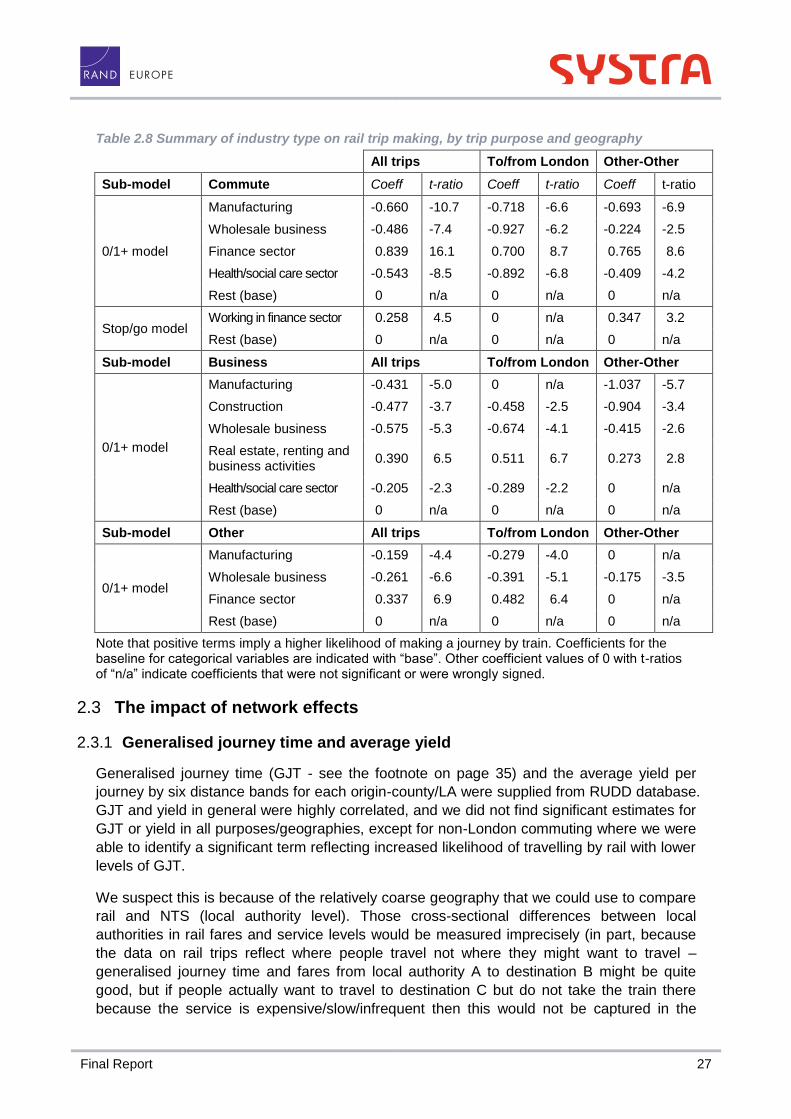
Final Report 27
Table 2.8 Summary of industry type on rail trip making, by trip purpose and geography
All trips To/from London Other-Other
Sub-model Commute Coeff t-ratio Coeff t-ratio Coeff t-ratio
0/1+ model
Manufacturing -0.660 -10.7 -0.718 -6.6 -0.693 -6.9
Wholesale business -0.486 -7.4 -0.927 -6.2 -0.224 -2.5
Finance sector 0.839 16.1 0.700 8.7 0.765 8.6
Health/social care sector -0.543 -8.5 -0.892 -6.8 -0.409 -4.2
Rest (base) 0 n/a 0 n/a 0 n/a
Stop/go model Working in finance sector 0.258 4.5 0 n/a 0.347 3.2
Rest (base) 0 n/a 0 n/a 0 n/a
Sub-model Business All trips To/from London Other-Other
0/1+ model
Manufacturing -0.431 -5.0 0 n/a -1.037 -5.7
Construction -0.477 -3.7 -0.458 -2.5 -0.904 -3.4
Wholesale business -0.575 -5.3 -0.674 -4.1 -0.415 -2.6
Real estate, renting and business activities
0.390 6.5 0.511 6.7 0.273 2.8
Health/social care sector -0.205 -2.3 -0.289 -2.2 0 n/a
Rest (base) 0 n/a 0 n/a 0 n/a
Sub-model Other All trips To/from London Other-Other
0/1+ model
Manufacturing -0.159 -4.4 -0.279 -4.0 0 n/a
Wholesale business -0.261 -6.6 -0.391 -5.1 -0.175 -3.5
Finance sector 0.337 6.9 0.482 6.4 0 n/a
Rest (base) 0 n/a 0 n/a 0 n/a
Note that positive terms imply a higher likelihood of making a journey by train. Coefficients for the baseline for categorical variables are indicated with “base”. Other coefficient values of 0 with t-ratios of “n/a” indicate coefficients that were not significant or were wrongly signed.
2.3 The impact of network effects
Generalised journey time and average yield 2.3.1
Generalised journey time (GJT - see the footnote on page 35) and the average yield per
journey by six distance bands for each origin-county/LA were supplied from RUDD database.
GJT and yield in general were highly correlated, and we did not find significant estimates for
GJT or yield in all purposes/geographies, except for non-London commuting where we were
able to identify a significant term reflecting increased likelihood of travelling by rail with lower
levels of GJT.
We suspect this is because of the relatively coarse geography that we could use to compare
rail and NTS (local authority level). Those cross-sectional differences between local
authorities in rail fares and service levels would be measured imprecisely (in part, because
the data on rail trips reflect where people travel not where they might want to travel –
generalised journey time and fares from local authority A to destination B might be quite
good, but if people actually want to travel to destination C but do not take the train there
because the service is expensive/slow/infrequent then this would not be captured in the

28 Rail Demand Forecasting Estimation
RUDD data) and may well be insignificant compared to the differences between parts of the
same local authority.
Access times to the station 2.3.2
Table 2.9 summarises the impact of bus and walk access times to the nearest rail station on
rail trip making. Across all purposes and most of the geographies, we observe that increase
in access times leads to a decrease in the propensity to make rail trips. However, we did not
observe a significant walk access time effect on London rail business trips and a significant
bus access time effect on the rest of the country business travel.
Table 2.9 Summary of walk and bus access times on rail trip making
All trips To/from London Other-Other
Sub-model Commute Coeff t-ratio Coeff t-ratio Coeff t-ratio
0/1+ model
Walk time to the nearest rail station
-0.020 -18.1 -0.007 -5.1 -0.022 -12.6
Bus time to the nearest rail station
-0.011 -5.2 -0.013 -4.2 -0.010 -3.1
Sub-model Business All trips To/from London Other-Other
0/1+ model
Walk time to the nearest rail station
-0.004 -4.4 0.000 n/a -0.004 -3.5
Bus time to the nearest rail station
-0.009 -3.9 -0.011 -4.1 0 n/a
Sub-model Other All trips To/from London Other-Other
0/1+ model
Walk time to the nearest rail station
-0.011 -22.6 -0.006 -7.2 -0.006 -7.2
Bus time to the nearest rail station
-0.010 -9.7 -0.010 -5.5 -0.010 -5.5
Note that positive terms imply a higher likelihood of making a journey by train.
2.4 Time trend effects
A simple linear time-trend variable is incorporated in the NTS models. The resulting term is
positive (and significant) for the 0/1+ model across most purposes and geographies,
indicating an increased likelihood of travelling by rail over time that is not explained by socio-
economic and network terms. Piecewise linear terms were also explored to test whether
there were differences in trends before and after 20061. For commute and other travel
differences in time trends before and after 2006 were not significantly different. For business,
we did observe that the time-trends are significantly different between before (includes 2006)
and after 2006. The time-trend coefficient for years up to 2006 was constrained to zero
because of insignificance but the term for years after 2006 is significant.
In all models, constants were also included for 2001, which reflected the much lower rail
travel levels in 2001 relative to other years, presumably because of the Hatfield rail accident.
1 We hypothesised that there is an increase in trip-rate sometime in mid 2000s, which may be because of technological advancements that have enabled working while travelling by train etc. To investigate this effect, we plotted the observed and predicted trip-rates by year for each purpose and identified a jump in rail trip rates for business travel after 2006. We tested a piece wise specification in our model specification breaking at years 2005, 2006 and 2007. However, the identified effect is significant for years after 2006 for business rail travel only.

Final Report 29
For business a constant is also included for 1999, which reflects higher rail travel in that year.
This may be a result of subsequent changes to company car ownership taxation benefits.
Table 2.10 Summary of time trends on rail trip making, by trip purpose and geography
All trips To/from London Other-Other
Sub-model Commute Coeff t-ratio Coeff t-ratio Coeff t-ratio
0/1+ model Btime 0.049 9.1 0.003 0.5 0.041 4.7
Stop/go model btime_S 0 n/a 0 n/a 0 n/a
Sub-model Business All trips To/from London Other-Other
0/1+ model btime (2006+) 0.039 4.2 0.047 4.2 0 n/a
Stop/go model btime_S 0.033 4.0 0.031 2.3 0.053 2.8
Sub-model Other All trips To/from London Other-Other
0/1+ model Btime 0.046 22.2 0.048 12.4 0.033 11.2
Stop/go model btime_S 0 n/a 0 n/a 0 n/a
Note that positive terms imply a higher likelihood of making a journey by train.
The size of these time trend terms, measured as the average increase on rail trip rates, is
illustrated in Table 2.11.
Table 2.11 Size of time trend terms (average increase in the overall rail trip rate)
Purpose Overall time trend To/from London Other-Other
Commute 2.6% 0% 4.0%
Business 3.9% 3.9% 0.8%
Other 4.3% 4.9% 3.2%
2.5 Outputs to models derived from ticket sales (RUDD models)
Trip rates were computed for specific classes of traveller types, for example by age group or
occupation type, to match available information in the RUDD database, which was used for
developing the rail demand models. An illustrative trip rate model that allows this for three
age groups and two occupation groups for explanation purposes is given below:
𝑇 = 𝛼0 +𝛼2𝐷𝐴2+𝛼3𝐷𝐴3 + 𝛼5𝐷𝑂2
Where D is a variable for age group 2 (A2), age group 3 (A3) and occupation group 2 (O2).
The α0 parameter reflects a base level of trip making to which there are incremental effects
for n-1 of n categories of each variable.
Predicted trip rates from the NTS travel frequency models 2.5.1
A two-step approach was used to obtain the model predicted trip-rates. First the model was
used directly to predict the alternative chosen in the travel frequency model (Equation 1 in
Appendix A), and then in a second step a calibration factor1 (odd/even ratio) defined as the
ratio between the total number of observed trips and the alternative chosen in the travel
frequency model is introduced to re-scale the total trips to the total number of observed trips.
1 It is assumed that the odd/even fraction is the same for all stop/go alternatives, i.e., alts 1_2, 3_4, 5_6 etc.. respectively. The calibration factor is less than or equal to one.

30 Rail Demand Forecasting Estimation
The trip rates from NTS models were extracted for the set of socio-economic variables which
are common to RUDD and NTS databases and are detailed in Annex A. The full set of trip
rates for each purpose and geography combination are summarised in section 3.2.

Final Report 31
3 Ticket Sales Analysis
3.1 Introduction
We now turn to the second modelling element of the study; developing new rail demand
models based on analysis of ticket sales data with the aim of providing a better
understanding of rail demand in recent years and a more robust basis for forecasting.
This chapter deals with how we went about developing improved rail demand forecasting
models, highlighting what we regard to be the key achievements. The next chapter delivers
the results of the modelling work.
In summary, the key features and outcomes of the models we have estimated and the
innovations we have made are as follows:
Extending coverage of conventional rail demand models based on ticket sales data to include a wider range of socio-economic impacts in a manner that provides credible and usable results.
Commissioning complementary analysis, of what can only be regarded as under-exploited NTS data, to provide quantitative insights that were not otherwise available and which enable the enhancement of conventional rail demand models.
Using the NTS data to improve the historical representation of variables in our rail demand models and also to account for switching between season and non-season tickets as a result of changes in the employment market.
Providing updated estimates of elasticities within the current PDFH framework.
Generally obtaining a better fit to the data and achieving superior back-casting performance.
The analysis of data pooled across directions of travel on routes where single leg tickets, such as advance, are now common is a long overdue development and may have contributed to obtaining more robust estimates.
Learning from the experiences of previous studies and constraining some parameter estimates to best available evidence given that unconstrained estimation can lead to unsatisfactory results. This procedure is supported with evidence that such an approach is essential here.
Extending the coverage of the Non London seasons ticket market from 20 to 50 miles, which is more in line with the Network Area and better represents current commuting patterns.
The provision of what seems like credible elasticity evidence for non-season trips within PTE areas where there is a dearth of reliable evidence.
The inclusion of employment related terms that plausibly account for the previously neglected issue of commuting on non-season tickets.
In response to concerns regarding structural changes in the employment and leisure markets, and in particular employment and leisure opportunities being increasingly focused around the regional centres, we have pursued the recently introduced distinctions relating to urban hierarchy. Moreover, we have successfully introduced local unemployment levels into season ticket models.

32 Rail Demand Forecasting Estimation
Allowance for trend increases in rail demand, as best we are able in the absence of clear evidence, due to the digital revolution which can be expected to have reduced the disutility of rail travel time at least relative to other modes and perhaps in absolute.
Given some unexplained and significant increases in rail demand in recent years, particularly in the immediate post 2008 recession period, we were keen to consider the possible contributions of otherwise unaccounted influences on rail demand. Two such factors that we explored were rolling stock improvements and gating.
The allowance for commuters switching between season and ordinary tickets as indicated from inspection of the NTS data.
3.2 Scope
We here explain the scope of the econometric work. There are two key issues we wish to
bring out here. Firstly, the categories of flows upon which the analysis has been based.
Secondly, the dimensions of the demand we have examined.
Scope of Analysis 3.2.1
The spatial coverage of our analysis is set out in Table 3.1, with the flow types covered
constituting the vast majority of rail revenue in Great Britain. The table also details the rail
tickets to which the analysed demand data relates, illustrating that we have not
disaggregated the non-season tickets into their constituent types nor distinguished by class
of travel.
Given that we are primarily concerned with the effects of external factors on rail demand, our
view is that finer disaggregation than the conventional distinction of season and non-season
(‘ordinary’) tickets would significantly add to the complexity of the task and would not add
great value to understanding of the key drivers of commuting and other travel except in the
unlikely event that ticket type choice could be very well explained. Phase 1 of the study
identified that there were movements in the spread of demand between ticket types over the
time period; we consider that this is likely to have been caused by the changing availability of
advance tickets and the changing restrictions on full tickets rather than changes in trip-
making behaviour in discrete markets for each ticket type.
We should though note that our enhancement of rail demand models with evidence relating
to socio-economic factors does distinguish journey purpose.
Table 3.1 Flows Examined and Specification of Demand
Flow Type Ticket Type Dimension Flows
London Long Distance
Non-Seasons Bi-directional Flows are to and from Central London
Non London Long Distance
Non-Seasons Bi-directional Includes Network Area Non London long distance
Non London Short Distance
Seasons
Non-Seasons Uni-directional Seasons extended to 50 miles
Network Area to London
Seasons
Non-Seasons
Uni-directional
Uni-directional
Seasons to Central London. Non-Seasons to and from Central London

Final Report 33
We have not covered the London Travelcard area since the widespread use of zonal tickets
means that the point-to-point demand data in LENNON is not an accurate guide to rail
demand.
For the same reason, there is general reluctance in rail ticket sales modelling to cover flows
entirely within PTE (Metropolitan1) areas. What we have here done is to include flows
entirely within PTE areas for non-season tickets, but allowing relevant parameters to vary
between the within PTE flows and all other flows. However, casual inspection of the season
ticket sales data for within PTE flows revealed it to have considerable volatility such that it
would not provide a firm basis for analysis and hence we have excluded it from our models.
A particularly important factor here is that point-to-point seasons are almost absent on West
Midlands and Merseyside flows over the period whilst elsewhere there seems to have been
significant variations in the relative attractiveness of point-to-point and PTE products over
time.
As part of inspecting the Non London short distance data, we observed, as might be
expected, large and ‘well-behaved’ season ticket demand on flows exceeding the 20 mile
limit of short distance used in PDFH. We therefore proceeded to analyse season ticket
demand for flows up to 50 miles outside of PTE areas in addition to the conventional short
distance non-PTE flows. The latter are those entirely outside a PTE area, between two
different PTE areas or with only one end in a PTE area.
With regard to trips between outside the and inside of the London Travelcard area, the within
Travelcard area is restricted to Central London as forming by far the largest demand and
revenue. Some of the smaller flows to and from locations within the Travelcard area exhibit
high levels of demand variability. As far as season tickets are concerned, the analysis has
been restricted just to trips to Central London, partly on the grounds that this is where the
employment data is more detailed and reliable but also because to Central London sales
dominate seasons demand and revenue.
Traditionally, econometric models based on rail ticket sales data have distinguished by
direction of travel, for very sound reasons. So the demand data recorded for trips apparently
originating in, say, Leeds and ending in London has been entered as separate observations
in the models alongside the equivalent demand data for the reverse direction. This can be
justified where rail travellers predominantly buy round trip tickets since, say, a cheap day
return or off-peak ‘Saver’ ticket bought in Leeds to travel to London and back can be
reasonably assigned to someone living in Leeds travelling to London and back. The same
applies to open return tickets sold in Leeds to travel to London and back.
And it then makes sense to distinguish by direction because it doubles the amount of data in
the model, the variations in fares, timetable related service quality and indeed exogenous
variables might vary by direction adding to the richness of the data and, importantly, the
characteristics of the market (demand elasticities) might also vary by direction.
1 The Metropolitan Counties of Strathclyde, Tyne & Wear, West Yorkshire, South Yorkshire, Greater Manchester, Merseyside and the West Midlands have (or had) Passenger Transport Executives (PTEs). These have (or had) important influences on rail services in their areas. In their areas they developed important multi-modal tickets that are much less important (or non-existent) elsewhere. These areas also have generally different rail services from other areas:more railway lines with more stations, higher frequency services and (often) lower fares.

34 Rail Demand Forecasting Estimation
Phase 1 of the study recognised that this is no longer a sensible approach on some routes.
The widespread use of single leg ‘advance’ tickets means that ticket sales origin-destination
data can no longer be considered to represent a production-attraction format. This approach
has nevertheless persisted until quite recently and could be the reason for some of the poor
results that our literature review reveals have been obtained.
We have therefore pooled data across directions on the London and Non London long
distance flows where we do not have a good way of distinguishing within, say, Leeds to
London tickets those who are residents of Leeds travelling to London and those who are
residents of London returning home from Leeds.
We can though be confident that for our other flows the directionality aspect is reasonably
accurate. Season ticket data typically reveals that the demand originating in, say, Southend
and travelling to London overwhelmingly exceeds the reverse flow, which is precisely what
we would expect. For shorter distance Non London flows, season ticket data as with London
flows tends to exhibit sensible relativities, being much larger for, say, Harrogate to Leeds
than the reverse. In the short distance non-seasons market, return tickets remain prevalent.
Whilst we have distinguished between season and non-season tickets, we have not
disaggregated the latter by the anytime, off-peak and advance categories and nor have we
distinguished between first and standard class. This is because to do so brings a whole set
of additional challenges, such as increasing availability and awareness of advance purchase
tickets over time and changes in restrictions to off-peak tickets which are confounded with
other variables, and particularly with GVA growth and to a lesser extent employment growth
which are central to this research.
Scope of Socio-Economic Variables 3.2.2
Collecting fresh data to enable a better understanding of rail demand trends was largely
outside the scope of this study.
So whilst many commentators have argued for employment data split by occupation type
with a geographical definition relevant to rail stations rather than local authority districts, or
for data on car parking costs and availability, or for more detailed income data for residents
nearer to stations, such data on the historical basis necessary for modelling is not readily
available.
We have though attempted to improve some historical data sets through our complementary
analysis of NTS data – this is described in Annex C.
We extracted from RUDD a wide range of socio-economic data to be used in the
econometric analysis. The emphasis was upon data which can make use of the insights
obtained from the NTS analysis into how socio-economic variables influence individuals’
propensities to make rail trips. The data is assembled for each flow and year as available.
Annex B provides a complete list of the socio-economic data that we were working with. In
summary, this socio-economic data is:
GVA and GDI per capita at NUTS3 level
Population in district, and split by five age bands

Final Report 35
Employees, both residence and workplace based at district level, and segmented by 9 occupation groups and 6 employment sector groups
The proportion of households at district level with no cars, 1 car, 2 cars or 3 or more cars
The proportion of full licence holders
Whilst other data is available in RUDD, it is of little use in our modelling since either it varies
little over time and across flows, such as gender split, or we are not in a position to exploit it
since we did not identify insights from NTS analysis, such as ethnic mix, because the
variable is missing from NTS or because it is likely to be correlated with other explanatory
variables.
Additional Explanatory Variables 3.2.3
In addition to the socio-economic variables, we have the standard industry data covering rail
revenue and demand, GJT1 and its constituent parts, and average minutes late.
We also assembled other data, within the limited resources available to us, which could be
useful in explaining rail demand. In addition to the improved data on historical car times and
costs derived from NTS as discussed in Annex C, we also added evidence on:
Gating
Rolling stock improvement
Disruptions due to West Coast Main Line upgrade
We felt that gating and rolling stock improvements could possibly have contributed to the
resilience of rail demand in the period of economic downturn post 2008; the gating and
rolling stock data are described in Annex C. Two potentially important variables that we do
not have historic information on are variations in crowding levels and the extent to which rail
travellers can use their travel time in a more worthwhile manner due to technological
developments.
3.3 Enhancing Rail Ticket Sales Models with NTS Trip Rate Evidence
Background and Approach 3.3.1
The background to this is that PDFH v4.0 in 2002 introduced a forecasting framework that
went far beyond the simple GDP elasticity and time trend that had been used for external
factors up to that point. It removed the time trend and introduced a car ownership term and a
series of inter-modal cross-elasticities. This was to a large extent inspired by the forecasting
approach advanced by Steer Davies Gleave (1999) in their National Passenger Demand
Forecasting Framework (NPDFF) study.
The problem with such a framework, as our Phase 1 literature review identified, is that a
consistent set of demand elasticities requires some form of joint estimation, since the
1 Generalised Journey Time, GJT, is a measure of rail service level for each origin-destination pair (flow) which is composed of station-to-station journey time, the inconvenience in time units of not being able to travel at the exact desired time and a time penalty for having to interchange. This measure is an average across the day and depends upon desired departure time profiles and assumptions regarding what represents an ‘opportunity to travel’ between O-D pairs.

36 Rail Demand Forecasting Estimation
variables are highly correlated, and this correlation itself causes problem in estimation, as
the literature review also pointed out with reference to a number of studies.
One solution to this problem, eventually reported in Wardman (2007), was to add historical
data on car ownership, car time and fuel costs alongside the rail and GDP data and
constrain the elasticities of the former three terms along with the population elasticity to the
best available evidence. Without such constraints, the entire set of freely estimated results
were simply not credible, yet imposing the constraints yielded a plausible GDP elasticity
which was also consistent with the constrained terms.
In this study we demonstrate, in section 3.4.3, that the estimation of parameters to only a
few key external factors within the existing framework is fraught with difficulty. This therefore
confirms the need to constrain some elasticities to what we regard to be the best available
evidence.
The discussion thus far is related to the approach adopted in the early 2000s for obtaining
an improved understanding of rail demand by incorporating additional terms in conventional
rail demand models that explicitly dealt with inter-modal competition. But we need to go
beyond this.
The method adopted in this study to obtaining a better explanation of rail demand extends
the existing approach to include a broader range of socio-economic variables. The Phase 1
review revealed that commentators were suggesting that structural changes in the labour
market and population towards locations, jobs and people with a greater propensity to use
rail could be a key driver of the strong rail commuting demand growth that had been
witnessed, as could more regionalised focus on shopping, recreational and entertainment
offerings in the non-seasons market1. But regardless of such comments, surely a natural
progression of existing rail demand models is to cover a wider range of socio-economic,
demographic and employment influences?
The extension of the current modelling framework to cover more socio-economic and
demographic factors brings its own set of challenges.
In attempting to enhance existing models, we could in some way include the key socio-
economic variables of interest set out above, and listed in the Phase 1 Report, into our
regression models of rail demand. The expected problem is that some parameter estimates
would be implausible or insignificant. In part this would be due to large correlations (or
limited variation) over time between key variables at the aggregate level at which our
demand models operate, such as between the different age and car ownership categories or
between the proportions in different occupation types and employment sectors and the
district level economic indicators. As an example, we experimented with different population
terms for the proportion in different age categories, and also in different occupation types.
The results were entirely unsatisfactory; we found large variations in elasticities across
specific population terms and indeed some being wrong sign. Again, therefore, there is a
need to make use of best available evidence on relevant parameters to support the analysis.
1 Historic data to support econometric analysis of how rail trips have been impacted by changes in entertainment, shopping, recreational and indeed employment opportunities, particularly in the large regional centres, is not readily available. This has resulted in the use of proxy terms, such as specifying incremental effects on demand elasticities for trips to major and particularly core cities.

Final Report 37
We recognise that rail trip rates vary considerably across people with different socio-
economic characteristics. This is so for different journey purposes. The NTS data provides a
rich source of information on trip rates and socio-economic characteristics and hence offers
the potential, as illustrated in the analysis reported in Chapter 2, to provide important insights
into rail trip making as a function of socio-economic variables that can be used to enhanced
ticket sales models.
There is precedence of using NTS data to inform rail demand: for example, the non-car
ownership term in the current PDFH recommendations was obtained from analysis of NTS
trip rates as a function of car ownership levels whilst the Wardman (2007) study reported rail
demand models based upon NTS data.
Specifically, the NTS data quantifies how the propensity to make rail trips varies across the
population. It therefore makes sense to create a population weighted index, with a given
population generating more or less rail trips according to its particular characteristics. An
attractive approach would be some kind of sample enumeration method, so that for any
location the local socio-economic characteristics are entered into the NTS model to yield an
expected trip rate.
Since the NTS data and analysis relates to the trips of individuals, it is possible to use the
model to obtain trip rates for any combination of socio-economic variables in the estimated
models. It can provide estimated trip rates for, say, those who are in age group 30-44 with a
professional occupation in the finance sector and 2 cars in their household, or who are aged
45-64 in a skilled trade in the manufacturing sector with a single car in their household, and
so on covering all permutations of age groups, occupations, employment sectors and car
ownership levels.
However, we cannot operate at this level of resolution with our ticket sales model. Whilst we
have, at district level, distributions of age group, occupation, employment type and car
ownership, we do not have cross-classifications of these variables (some of the cells would
be very small). Thus we must operate with each variable separately at the level of
aggregation in RUDD, which will tend to reduce the amount of variation across districts
compared to a sample enumeration approach.
The approach adopted was therefore to determine how trip rates vary from the average
according to each category of the socio-economic variables available in RUDD: specifically
by age group, occupation, employment sector, licence holding status and household car
ownership. The NTS models were used to determine average rail trip rates for the different
categories within each of these variables. Thus we obtain implied average leisure trip rates
for those in, say, the 15-29 age group or those with 1 car. These trip rates were then applied
to the proportion of the local population in each category to determine expected trip rates for
the local population.
The Expected Trip Rates 3.3.2
We have gone down the path of calculating an index which determines how rail trip rates
vary from what is the expected trip rate.
Tables 3.2, 3.3 and 3.4 present the predicted rail trip rates per week per person by the key
variables we can use in RUDD for commuting trips, other trips and business trips

38 Rail Demand Forecasting Estimation
respectively. In each case, a distinction is made between trips to and from London and other
trips.
The average rail trip rate per week per person is given in the third row in each table. This
figure has been used in calculating the deviation from the mean trip rate of each category.
So for commuters in the 30-44 category for Non London trips, the mean trip rate is 0.0917
which, given an average trip rate of 0.0879, results in a deviation from the mean of 0.0038.
In Tables 3.2 and 3.4, there are no observations for those under 15 as the trips relate to
employment. As expected, within any variable there are positive and negative deviations
across the different categories.
Table 3.2 Implied Commuting Trip Rates, derived from NTS rail trip rate models
To/from London Non London
Category Segment Trip Rate Deviation Trip Rate Deviation
Average All 0.0790 - 0.0879 -
Age <15 - - - -
15-29 0.0669 -0.0121 0.1299 0.0420
30-44 0.0983 0.0193 0.0917 0.0038
45-64 0.0705 -0.0085 0.0609 -0.0270
65+ 0.0334 -0.0456 0.0286 -0.0593
Occupation Managers and senior officials 0.1626 0.0836 0.1191 0.0312
Professional occupation 0.1644 0.0854 0.1362 0.0483
Associate professional 0.1210 0.0420 0.1292 0.0413
Administrative occupation 0.0845 0.0055 0.1461 0.0582
Skilled trade 0.0285 -0.0505 0.0375 -0.0504
Personal service 0.0211 -0.0579 0.0445 -0.0434
Sales and customer service 0.0184 -0.0606 0.0552 -0.0327
Process, plant and machine 0.0291 -0.0499 0.0411 -0.0468
Elementary occupations 0.0242 -0.0548 0.0553 -0.0326
Sector Manufacturing 0.0396 -0.0394 0.0453 -0.0426
Construction 0.0580 -0.0210 0.0595 -0.0284
Wholesale 0.0255 -0.0535 0.0673 -0.0206
Financial 0.1995 0.1205 0.1649 0.0770
Public admin 0.0656 -0.0134 0.0857 -0.0022
Other 0.0838 0.0048 0.0922 0.0043
Licence No licence 0.0514 -0.0276 0.1592 0.0713
Full licence 0.0851 0.0061 0.0735 -0.0144
Car 0 cars 0.0888 0.0098 0.1824 0.0945
1 car 0.0831 0.0041 0.1102 0.0223
2 cars 0.0812 0.0022 0.0638 -0.0241
3+ cars 0.0609 -0.0181 0.0491 -0.0388

Final Report 39
Table 3.3 Implied Business Trip Rates, derived from NTS rail trip rate models
To/from London Non London
Category Segment Trip Rate Deviation Trip Rate Deviation
Average All 0.0206 0.0119
Age <15 - - - -
15-29 0.0126 -0.0080 0.0096 -0.0023
30-44 0.0250 0.0044 0.0134 0.0015
45-64 0.0218 0.0012 0.0120 0.0001
65+ 0.0160 -0.0046 0.0096 -0.0023
Occupation Managers and senior officials 0.0509 0.0303 0.0238 0.0119
Professional occupation 0.0507 0.0301 0.0266 0.0147
Associate professional 0.0354 0.0148 0.0219 0.0100
Administrative occupation 0.0055 -0.0151 0.0055 -0.0064
Skilled trade 0.0074 -0.0132 0.0048 -0.0071
Personal service 0.0042 -0.0164 0.0054 -0.0065
Sales and customer service 0.0034 -0.0172 0.0043 -0.0076
Process, plant and machine 0.0072 -0.0134 0.0048 -0.0071
Elementary occupations 0.0050 -0.0156 0.0052 -0.0067
Sector Manufacturing 0.0173 -0.0033 0.0040 -0.0079
Construction 0.0096 -0.0110 0.0039 -0.0080
Wholesale 0.0063 -0.0143 0.0064 -0.0055
Financial 0.0474 0.0268 0.0224 0.0105
Public admin 0.0147 -0.0059 0.0126 0.0007
Other 0.0235 0.0029 0.0134 0.0015
Licence No licence 0.0094 -0.0112 0.0104 -0.0015
Full licence 0.0231 0.0025 0.0122 0.0003
Car 0 cars 0.0182 -0.0024 0.0138 0.0019
1 car 0.0188 -0.0018 0.0120 0.0001
2 cars 0.0226 0.0020 0.0115 -0.0004
3+ cars 0.0222 0.0016 0.0110 -0.0009

40 Rail Demand Forecasting Estimation
Table 3.4 Implied Other Trip Rates, derived from NTS rail trip rate models
To/from London Non London
Category Segment Trip Rate Deviation Trip Rate Deviation
Average All 0.0267 - 0.0618 -
Age <15 0.0140 -0.0127 0.0539 -0.0079
15-29 0.0377 0.0110 0.1112 0.0494
30-44 0.0359 0.0092 0.0595 -0.0023
45-64 0.0257 -0.0010 0.0428 -0.0190
65+ 0.0170 -0.0097 0.0448 -0.0170
Occupation Managers and senior officials 0.0448 0.0181 0.0432 -0.0186
Professional occupation 0.0581 0.0314 0.0773 0.0155
Associate professional 0.0517 0.0250 0.0691 0.0073
Administrative occupation 0.0308 0.0041 0.0656 0.0038
Skilled trade 0.0135 -0.0132 0.0385 -0.0233
Personal service 0.0213 -0.0054 0.0601 -0.0017
Sales and customer service 0.0192 -0.0075 0.0844 0.0226
Process, plant and machine 0.0067 -0.0200 0.0363 -0.0255
Elementary occupations 0.0202 -0.0065 0.0680 0.0062
Sector Manufacturing 0.0153 -0.0114 0.0451 -0.0167
Construction 0.0198 -0.0069 0.0445 -0.0173
Wholesale 0.0177 -0.0090 0.0597 -0.0021
Financial 0.0478 0.0211 0.0626 0.0008
Public admin 0.0309 0.0042 0.0591 -0.0027
Other 0.0267 0.0000 0.0668 0.0050
Licence No licence 0.0216 -0.0051 0.0776 0.0158
Full licence 0.0306 0.0039 0.0497 -0.0121
Car 0 cars 0.0291 0.0024 0.0841 0.0223
1 car 0.0265 -0.0002 0.0623 0.0005
2 cars 0.0273 0.0006 0.0520 -0.0098
3+ cars 0.0222 -0.0045 0.0474 -0.0144
The Trip Rate Indices 3.3.3
The aim is to weight the determinant of trip making according to the propensity of individuals
to make rail trips.
For non-commuting trips, we use the expected trip rate index to weight the origin population.
Given that employment drives commuting trips, we use the expected trip rate index to weight
employment at the destination.
The expected trip rate per person per week is calculated using the mean trip rate and
adjusting it according to the deviations in Tables 3.2 to 3.4 for the proportion of the
population in each category.
Doing the calculation just for leisure trips on Non London flows and for the age distribution,
we would have an expected trip rate (ETR) on a particular flow and year of:

Final Report 41
𝐸𝑇𝑅 = 0.0618 + (−0.0079 × 𝑃𝐴1) + (0.0494 × 𝑃𝐴2) + (−0.0023 × 𝑃𝐴3)
+ (−0.0190 × 𝑃𝐴4) + (−0.0170 × 𝑃𝐴5)
where 𝑃𝐴1 , 𝑃𝐴2 , 𝑃𝐴3 , 𝑃𝐴4 , and 𝑃𝐴5 are the proportion of the population in age groups 1-5
relevant to the flow and year in question.
To this are then added the deviations for occupation, employment sector and car ownership
level to obtain an overall ETR. We did not persist with the licence holding term since we felt
it did not add a great deal over and above car ownership; further, it complicates the
forecasting framework, not least because (unlike car ownership) there are no known
forecasts available.
The index used to weight either population or employment to allow for socio-economic
factors (INDEXSE) is derived as:
𝐼𝑁𝐷𝐸𝑋𝑆𝐸 = 𝐸𝑇𝑅
𝑀𝑇𝑅
where MTR is the mean trip rate, which is 0.0618 in the above example. In the calculations
here, the same MTR is used across all years.
A further elaboration was to allow for the variations in trips across individuals due to
variations in income. Analysis of the NTS data provided cross-sectional income elasticities
and these are set out in Table 3.5. As expected, the propensity to make rail trips is greater
for those with higher incomes, and this is in addition to employment sector, occupation and
car ownership effects. Not surprisingly, we obtain higher income elasticities on London flows
although the magnitude of them raises concerns that they are not entirely independent of
variations in income over time.
Table 3.5 Cross-Sectional Income Elasticities from NTS Analysis
Purpose London Non London
Commuting 1.47 0.22
Business 1.46 0.79
Other 0.86 0.07
The adjustment applied for income variations (INC_ADJ) was based on gross disposable
income (GDI). It took the following form:
𝐼𝑁𝐶𝐴𝐷𝐽 = [(𝐺𝐷𝐼𝑖
𝐺𝐷𝐼𝐴𝑉)
𝑦
× 𝑀𝑇𝑅] − 𝑀𝑇𝑅
where GDIi and GDIAV are respectively GDI for the station (NUTS3 area) and the average
across the country and y is the income elasticity. A modified index (INDEXSE_INC) is therefore
obtained as:
𝐼𝑁𝐷𝐸𝑋𝑆𝐸_𝐼𝑁𝐶 = 𝐸𝑇𝑅 + 𝐼𝑁𝐶𝐴𝐷𝐽
𝑀𝑇𝑅

42 Rail Demand Forecasting Estimation
Table 3.6 sets out how INDEXSE (and INDEXSE_INC) is calculated for each of the market
segments we incorporate in the ticket sales models.
For long distance journeys, we assume commuting to be a very small proportion of all trips1,
and indeed we have not included season ticket sales in our analysis of such flows. Hence
we operate with the trip rates for business and other travel. The appropriate London and
non-London trip rate evidence is used for the two long distance flow types. Given that on
these flows we are dealing with data aggregated across directions, we calculated the trip
rates for business and for other trips for each station and took the average. This is then
applied to the average population across the two stations. We allow for the business travel
trip rates applying only to the adult population.
Table 3.6 Calculation of Socio-economic Weighting (INDEXSE)
Flow Type Trip Rates Used Variable Weighted
London Long Sum of Business and Other averaged over both stations
Population averaged over both stations
Non London Long Sum of Business and Other averaged over both stations
Population averaged over both stations
Non London Short Seasons
Commuting Destination employment
Non London Short Non Seasons
Business and Other at origin station. Population at origin station.
Commuting from origin to destination (characteristics of population at origin and jobs at destination).
Destination employment
SE to London Seasons Commuting Destination employment
SE to London Non Seasons
Business and Other at origin station. Population at origin station.
Commuting from origin to destination (characteristics of population at origin and jobs at destination).
Destination employment
Turning to season ticket models for the Network Area to London and Non London short
distance, we use only the relevant commuting trip rate evidence from Table 3.2. We are here
dealing with trips disaggregated by direction and the weighting is applied to jobs at the
destination.
We have modified the specification of the weight here compared to the analysis of NTS data
which relates to the characteristics of the population that generate the trips (from the origin
station). The age distribution and the car ownership variables are related to the origin station
characteristics. However, we have linked the employment sector and occupation to the
distribution of jobs on offer at the destination.
The remaining two sets of flows specifically relate to non-season tickets, for Network Area to
and from London and Non London short distance travel, but they will include some
commuters who are not travelling on season tickets. This is may be because they do not
travel into work every day and hence the discounts offered by a season ticket do not provide
better value for money than buying day tickets. We therefore should cater for trip rates for all
journey purposes as part of our modelling enhancements to account for commuting on non-
season tickets. We initially set out weighting population by the trip rates for business, other
1 This is confirmed by our analysis in Annex B. The estimated trip rates do not distinguish by trip distance.

Final Report 43
and commuting. However, because commuting is determined by employment, we used two
separate indices; one weighting population and driven by business and other trips and the
other weighting employment and based around commuting trip rates.
There are approximations involved in this process of accounting for the effects of socio-
economic variables on rail trip rates whilst we are basing the expected trip rates on model
outputs which will themselves contain an element of error. It is therefore informative to
examine some properties of the measures we have constructed.
Table 3.7 reports summary statistic for INDEXSE for the six flow types. Given the
approximations involved, it is reassuring that in general the expected rail trip rates are
generally not greatly different from one. We might expect them to exceed one since our
locations are precisely those where the propensity to make rail trips will be highest and
generally greater than the mean across the country. This is presumably why the Network
Area to London seasons index is so large.
We also report in Table 3.7 a regression of INDEXSE_INC on a time trend to determine the
extent that allowing for socio-economic factors will have contributed to rail demand growth
over time. In all but one case, the index increases over time. However, it is only for “London
Long” and the two sets of Network Area flows where the growth is substantial whilst the Non
London short season flows where trip rates fall, although only with a very small effect.
Nonetheless, the index can still lead to improved understanding of rail demand by helping to
explain differential performance across different routes.
Table 3.7 Features of the INDEXSE Measure
Flow Type INDEXSE INDEXSE = α + β Trend
London Long 1.31 (0.10) [9747] α = 1.19 (811.5) β = 0.012 (93.3) R2 = 0.47
Non London Long 0.97 (0.06) [117496] α = 0.95 (2822) β = 0.002 (65.5) R2 = 0.04
Non Lon Short Seasons 1.21 (0.14) [35064] α = 1.22 (772.6) β = -0.001 (8.6) R2 = 0.01
Non Lon Short Non Seasons
0.98 (0.07) [69829] α = 0.98 (1588) β = 0.001 (16.1) R2 = 0.01
SE to London Seasons 1.71 (0.07) [8075] α = 1.62 (1391) β = 0.010 (92.9) R2 = 0.52
SE to London Non Seasons
1.40 (0.17) [15992] α = 1.29 (488.1) β = 0.011 (46.8) R2 = 0.12
Note: Mean, (standard deviation), [number of flow-year observations].
Table 3.8 reports the same results but for the income enhanced index (INDEXSE_INC). The
mean values are only really different for flows involving London and this is where the income
elasticities are largest. These are also the flows where even without the income effect the
propensity for making rail trips was, as expected, above average. The higher incomes for the
Network Area and for London based trip making merely strengthens this effect. The trend
effects are smaller for the Network Area flows and this may be because the income
elasticities contain a temporal effect.

44 Rail Demand Forecasting Estimation
Table 3.8 Features of the INDEXSE_INC Measure
Flow Type INDEXSE_INC INDEXSE_INC = α + β Trend
London Long 1.85 (0.17) [9747] α = 1.60 (712.6) β = 0.025 (127) R2 = 0.63
Non London Long 0.96 (0.06) [117496] α = 0.95 (2676) β = 0.002 (56.0) R2 = 0.03
Non Lon Short Seasons 1.22 (0.15) [35064] α = 1.23 (767.1) β = -0.001 (10.0) R2 = 0.01
Non Lon Short Non Seasons
0.99 (0.08) [69829] α = 0.98 (1550) β = 0.001 (12.4) R2 = 0.02
SE to London Seasons 1.95 (0.24) [8075] α = 1.88 (346.7) β = 0.008 (16.6) R2 = 0.05
SE to London Non Seasons
2.11 (0.71) [15992] α = 1.87 (163.6) β = 0.024 (24.3) R2 = 0.04
3.4 General Principles of Our Modelling
The Modelling Approach 3.4.1
We have estimated fixed effects regression models to our data pooled across routes and the
19 years of data between 1995/96 and 2013/14 available to us. These take the form:
Equation 1 Fixed effects regression model
𝑉𝑖𝑗𝑡 = 𝜏 ∏ 𝑋𝑖𝑗𝑘𝑡𝛼𝑘
𝑛
𝑘=1
𝑒∑ 𝛽𝑙𝑋𝑖𝑗𝑙𝑡𝑚𝑙=1 𝑒∑ 𝛾𝑟𝐷𝑖𝑗𝑟𝑡
𝑠𝑟=1
𝑉𝑖𝑗𝑡 is the demand for rail travel between stations i and j in time period t. It is a function of n
continuous variables ( 𝑋𝑖𝑗𝑘𝑡 ) entered so that their coefficients ( 𝛼𝑘) are interpreted as
elasticities and m continuous variables (𝑋𝑖𝑗𝑙𝑡) entered so that their coefficients (𝛽𝑙) denote
the proportionate change in demand after a unit change in the variable and the elasticity is
then proportional to the level of the variable ( 𝛽𝑙𝑋𝑖𝑗𝑙𝑡 ). In addition, there are 𝑠 discrete
variables denoted by the dummy variables (𝐷𝑖𝑗𝑟𝑡 ) and their coefficients (𝛾𝑟) denote the
proportionate effect on demand of a particularly category of a variable relative to an
arbitrarily selected base category.
Of course, this representation could be generalised to allow for interactions between
different continuous variables, between different categorical variables, or between discrete
and categorical variables.
A key feature of the model is the specification of dummy variables to represent p-1 of the p
station-to-station movements. These are covered by the 𝐷𝑖𝑗𝑟𝑡 term without any variation by
time period t. These ‘fixed effects’ represent any unobserved or unaccounted for
characteristics that are specific to each flow which do not vary over time, essentially allowing
flow specific intercepts with variations in demand then driven by variations in the explanatory
variables over time.
The reported models contain a large number of these fixed effect dummy variables, and over
90% of their coefficient estimates were significant at the 10% level. We did not remove in
each model estimated those that were not significant since this would have been a very
substantial task given that there is some variation in which fixed effects are significant across

Final Report 45
the different models examined. However, we did some testing of the sensitivity of the main
parameter estimates to the exclusion of insignificant fixed effects and found very little effect.
The continuous variables might be 𝑖-𝑗 flow specific, such as fare or GJT, origin specific, such
as population, GVA or car ownership levels, or destination specific, such as employment.
Upon logarithmic transformation of this equation, its parameters can be estimated by
ordinary least squares regression.
In all cases, we have adjusted prices in line with the CPI measure of inflation whilst GVA
was adjusted by the GDP deflator.
Some previous studies have experimented with removing data which was deemed to be of
poorer quality or considered to be misleading. Such a process is not without controversy if
the results depend strongly on the omission of observations. We have estimated models
which remove flows where there were large changes in demand or where the volume of
demand was low. This did not lead to great differences in results, and certainly not ones that
were markedly superior. We used weighted least squares, placing greater emphasis on
larger flows where the data might be regarded to be more reliable, but again this did not lead
to models which were deemed to merit retentions.
We would add that some of these data sets are extremely large, and hence identifying what
might be regarded to be unreliable data is not a straightforward task. We have instead opted
for removing observations with standardized residuals outside the range ±2. We feel this is
less arbitrary than selecting models which have had data removed on the ground that the
results look more appealing and the process will remove around 5% of observations which
can be regarded to be of lowest ‘quality’.
Nor have we placed much emphasis on conducting statistical tests compared to efforts at
model enhancement. The t ratios for key variables are generally so high that correction for
the presence of autocorrelation or heteroscedasticity would not materially alter the
confidence we can place in the parameter estimates and indeed many of the key parameters
in the estimated models are actually constrained. In passing, we note that Durbin Watson
statistics were routinely output in estimation and did not indicate the presence of strong
autocorrelation.
We have used constrained parameter estimation extensively, which was identified to be an
important process in the literature review, and it is to a discussion of these constraints that
we now turn.
Parameter Constraints 3.4.2
In addition to the constraints involved in adopting the insights provided by the NTS analysis
of socio-economic factors, we have also applied constraints to a number of other parameters
in our models. These are:
Population elasticity
Employment elasticity
GJT elasticity
Cross-elasticities between modes
46 Rail Demand Forecasting Estimation
Although we have allowed the population elasticity to be freely estimated, this does not
always yield plausible results, as was apparent in our literature review and, as we
demonstrate, also turned out to be the case here. The situation is similar for the employment
term.
When the population and employment elasticities are constrained, they are constrained to
one, on the grounds that we would expect, for a given socio-economic composition of the
population, commuting trips to vary in direct proportion to employment opportunities and
non-commuting trips to vary in direct proportion to population.
GJT elasticities are constrained to current PDFH recommendations. The need for the
constraints is discussed in section 5.4.3.
As for cross-elasticities between modes, our literature review clearly shows the need for
constrained parameter estimation and, in section 5.4.3, we confirm that such constraints are
required here. We have used historical NTS data, described in Annex C, regarding
competition from other modes:
Car time (based on NTS)
Car fuel cost including efficiency (based on NTS speed and DfT car cost curves)
Car cost which adds non-fuel costs to the fuel costs
Bus time (based on NTS)
Proportion of households without a car
We find the cross-elasticities in PDFH5.1 with regard to car fuel cost and car journey time to
be too large in several instances. If they really were as as the figures for car fuel
cost and sometimes or over for car time, which puts them on a par with some rail fare
elasticities, then we might have reasonably expected to have seen such figures reliably
estimated in the literature. We also note that own elasticities for car fuel cost and journey
time are less than some of the rail cross-elasticities with respect to those variables in PDFH!
Furthermore, our literature review in Phase 1 of the project identified a large number of
statistically significant elasticities of rail demand with respect to some form of car cost, and
they often do not support the figure of that PDFH recommends for almost all flow types.
Bearing in mind that some studies return insignificant elasticities, which would presumably
reflect actual elasticities at the low end, we feel that our Phase 1 literature review would
warrant a car fuel cost cross-elasticity of 0.25 in place of PDFH’s .
We also went back to the first study that included cross-elasticities in rail demand forecasting
frameworks (Steer Davies Gleave, 1999). That review of evidence also formed the basis of
PDFH v4 recommendations in this regard. These are set out in Table 3.9 and distinguish by
journey purpose; they are very similar to the current WebTAG recommendations. Our view is
that these figures fit our expectations and the preceding discussion better than PDFH v5.1
and hence we have adopted them here.

Final Report 47
Table 3.9 Cross Elasticities from National Passenger Demand Forecasting Framework
Flow Type Car Fuel Cost Car Time
Comm EB Leisure Comm EB Leis
London Long
Network Area to London
Non London Long
Non London Short
Given these figures are split by journey purpose, we have weighted them using NTS data
(the analysis is described in Annex B) to arrive at the set of cross-elasticities to car fuel cost
and car time to serve as constraints in our models as set out in Table 3.10.
Table 3.10 Constraints Used in Estimated Models
Flow Type Car Fuel Cost Car Time Car Ownership
PDFH Used PDFH Used PDFH Used
London Long 0.21 0.28 NTS
Non London Long 0.26 0.30 NTS
Non Lon Short Seasons 0.40 0.20 NTS
Non Lon Short Non Seasons
0.40 0.20 NTS
SE to London Seasons 0 0 NTS
SE to London Non Seasons
0.19 0.22 NTS
Table 3.10 also lists the PDFH recommended ‘non’ car ownership effects. Again, we feel
these to be generally on the side. In particular, when we simulated car ownership
changes within INDEXSE the impacts are than PDFH recommendations (although
INDEXSE also includes further impacts for further cars). Note, however, that the PDFH car
ownership effects are only included in our estimated models which do not contain INDEXSE
given that the latter includes car ownership.
We have included bus cross-elasticities in our models since, while we do have coarse data
on bus speeds, we do not have robust data on bus costs. This is not to say that we
recommend the exclusion of bus cross-elasticities from rail demand models, and we make
some recommendations in section 6.3.5.
The Need for Parameter Constraints 3.4.3
The Phase 1 literature review identified that all too often unacceptable results were obtained
in rail demand models when they attempted to estimate effects of a ‘wide’ range of external
factors. Indeed, we also observed implausible results in models that contained only a limited
set of external variables, such as a car fuel cost elasticity alongside GDP and also the
‘PDFH v3 approach’ of just a GDP elasticity and a time trend.
Given this had been a major issue in our assessment of previous evidence, and indeed
constrained parameter estimation was a key feature of our intended approach, it is beholden
upon us to test whether or not plausible result can be obtained with free estimation of
coefficients to such variables with the data at our disposal.

48 Rail Demand Forecasting Estimation
As can be seen from the results presented in Table 3.11, where the external factor
coefficients are freely estimated, there are a considerable number of unacceptable results in
terms of wrong sign or implausibly large effects even though the parameters are generally
estimated with a very high degree of precision. Unacceptable results persist even after
reducing the number of freely estimated external factors in the models.
These findings demonstrate the need for parameter constraints in model estimation. We
note though that the GDP and employment elasticities which are the most critical to
forecasting are noticeably the most robust and generally plausible.
Table 3.11 Examples of Freely Estimated Parameters for External Factors
Flow Type GVA/EMP Population Non-Car Ownership (NC)
Fuel Car Time
London Long 1.28 (15.3) 1.22 (6.7) 0.23 (1.4) -0.22 (5.6) 9.41 (4.2)
Non London Long 1.03 (95.4) 1.90 (115) -0.90 (25.9) 0.29 (33.1) 0.47 (23.3)
Non London Short Seasons
0.70 (22.4) n.a. -2.28 (23.4) 1.08 (40.3) 6.06 (32.8)
Non London Short Non Seasons
0.74 (57.4) 2.39 (74.8) -0.75 (19.1) 0.43 (36.5) 2.16 (31.5)
SE to London Seasons 1.27 (24.5) n.a. -0.18 (1.1) 0.24 (6.1) -0.85 (1.4)
SE to London Non Seasons
0.58 (20.3) 16.02 (19) 1.16 (11.2) 0.37 (15.5) 7.31 (19.7)
Note: These are from model formulations following PDFHv5.1 without any of the enhancements made in this study.
Our literature review focused on the need to constrain the parameters estimated to external
factors. A key influence on the demand for rail travel is what is termed Generalised Journey
Time (GJT) which is composed of station-to-station journey time, the inconvenience in time
units of not being able to travel at the exact desired time and a time penalty for having to
interchange.
This measure is an average across the day and depends upon desired departure time
profiles and assumptions regarding what represents an ‘opportunity to travel’ between O-D
pairs. Whilst GJT provides a reliable account of what might be regarded as ‘significant’
changes to timetables, be it journey time, service frequency or interchange requirements, it
can exhibit minor changes when the change in rail service level seems imperceptible. The
railway industry in Britain is continually striving to improve its offering, and often these are
quite marginal although building up to larger changes over time. So slight and trend
improvements as a result of, say, retiming some connections, changing departure times or
small improvements in journey time could correlate with the trend increases in rail demand
witnessed in Britain over many years and lead to exaggerated GJT elasticities. Moreover,
some new open access operators have offered only slight reductions in measured GJT but
have opened up new catchment areas and captured traffic from rival operators at other
stations, and this will lead to exaggerated GJT elasticities (because the GJT at the station
from which the demand is lost may not have changed).
We were therefore concerned when we obtained the freely estimated GJT elasticities
reported in Table 3.12, particularly given that the PDFH elasticities are explicitly long run

Final Report 49
whereas we are here dealing with a one-year response 1 . In addition, our previous
experiences have been that in the absence of ‘significant’ changes to timetables the GJT
elasticity has been low and insignificant whereas the large data sets here will facilitate the
recovery of coefficient estimates with high t ratios even with only trend improvements. They
will also capture stations where service level improvements have been associated with
changes in station choice: at some stations there will be an ‘excessive’ response to the
improved service, whereas at other stations the service level may not have changed but
demand lost.
Table 3.12 Freely Estimated GJT Elasticities (with t-statistics)
Flow Type GJT Elasticity PDFH Elasticity
London Long -1.88 (33.9)
Non London Long -1.65 (67.8)
Non Lon Short Seasons -1.58 (43.9)
Non Lon Short Non Seasons -1.31 (76.2)
SE to London Seasons -1.68 (23.9)
SE to London Non Seasons -1.44 (24.8)
We have therefore constrained the GJT elasticities in our estimated models to the PDFH
recommendations. Having said all this, imposing these GJT constraints made very little
differences to the other parameter estimates in our models.
The Impact of the Socio-Economic Indices 3.4.4
We have experimented with two indices as described in section 3.3.3. One of these includes
the effects on rail trip making of age group, employment sector, occupation type and car
ownership (INDEXSE) whilst the other additionally incorporates cross-sectional income
effects (INDEXSE_INC).
The approach we have used to enhance existing models is novel and can be preferred on
theoretical grounds as covering a wider range of variables that are widely expected to
influence rail demand. However, an important question that inevitably arises is whether the
use of these weights produces ‘better’ models. We interpret better models in two ways:
An improved statistical fit along with possibly more plausible parameter estimates
An ability to provide a better account of recent demand trends, fitting in with the strong emphasis on back-casting exercises in recent years.
Goodness of Fit and Parameter Estimates
We report here ‘standard’ PDFH models containing fare, GJT, GVA or employment,
population for non-commuting trips, car fuel cost and car time. GJT is constrained to PDFH
recommendations and the fuel cost and car time cross-elasticities are constrained to the
revised figures set out in Table 3.10. The population and employment elasticities are
constrained to one. The models are based on data after the removal of outliers although this
does not materially alter the findings.
1 The modelling did not progress to consideration of dynamic models and hence the demand response here is relevant to one year. The limited resources available for econometric modelling largely focussed on the possible enhancements due to the incorporation of a broader range of socio-economic effects.

50 Rail Demand Forecasting Estimation
The models reported in Table 3.13 are:
I: Standard population/employment model with additional car ownership term set to
PDFH recommendation
II: Standard population/employment model with car ownership effect set to zero
III: INDEXSE used to weight population/employment with car ownership set to zero
IV: INDEXSEINC used to weight population/employment and car ownership set to zero
Table 3.13 reports models for our six flow types and provides the residual sum of squares
and the estimated GVA or employment elasticity. The purpose of these models is to test the
impact of the socio-economic indices and the exact same models are not reported
elsewhere.
Models III and IV generally provide somewhat lower GVA or employment elasticities than
Models I and II. This is because the indices can explain demand growth that would otherwise
be incorrectly attributed to GVA or employment.
Model II removes what is often a large car ownership effect. In three out of five cases, this
leads to an improved fit although generally without a large impact on the GVA or
employment elasticity.
We note though that INDEXSEINC never provides a better fit than INDEXSE. Encouragingly,
INDEXSE provides the best fit in four of the six flow types, even though measurement error in
the socioeconomic data may introduce additional noise over and above measurement error
in population numbers.

Final Report 51
Table 3.13 Impact of Socio-Economic Indices
Flow Type Model RSS GVA/EMP
London Long I 454.76 1.64 (65.5)
II 456.87 1.65 (65.4)
III 461.12 1.24 (49.2)
IV 463.97 1.00 (39.6)
Non London Long I 4645.48 1.45 (179.1)
II 4552.65 1.30 (162.3)
III 4450.59 1.28 (161.6)
IV 4458.60 1.29 (161.7)
Non London Short Seasons
I 5608.56 1.83 (56.7)
II 5593.43 1.72 (54.5)
III 5564.56 1.27 (43.7)
IV 5583.96 1.24 (42.4)
Non London Short Non Seasons
I 3103.26 1.20 (113.2)
II 3019.73 1.08 (103.1)
III 2958.96 1.09 (105.0)
IV 2969.38 1.09 (104.8)
Network Area to London Seasons
I 301.28 1.40 (73.7)
II n.a. n.a
III 306.56 1.08 (72.1)
IV 314.15 1.10 (70.0)
Network Area to/from London Non Seasons
I 523.33 1.35 (65.1)
II 532.49 1.35 (64.6)
III 515.15 1.10 (53.9)
IV 548.03 0.82 (38.7)
RSS is the ‘residual sum of squares’; a lower number indicates better model fit (although values are not comparable between models). Note: For Network Area to London seasons, Model II is the same as Model I as the recommended car ownership parameter is zero.
Backcasting Evidence
In the backcast models, the improvement in model performance provided by using the
Socio-Economic indices appeared to be relatively modest. The increase in rail demand
provided by the socio-economic indices is gradual; the change represented is typically less
than 1% per year (for example Inner London population increases 1.3% p.a. during our data,
whereas the POPSE measure increases 2.0% p.a.). The growth provided is then offset by the
lower income and employment elasticities of the sort that can be observed in Table 3.13
above.
The socio-economic index can, nevertheless, be preferred on theoretical grounds – it is
important not to attribute these effects to increased income. Were favourable employment
and demographic trends not to continue, then we would overstate the growth in the rail
market that will come from income growth. In addition, we can reasonably expect the
enhanced models to provide a better account of differential performance across different
flows.

52 Rail Demand Forecasting Estimation
4 Estimated Ticket Sales Models
We here report our preferred models for each of the six sets of flows, arrived at after
exploring a large number of different variables and formulations. The preferred models
remove observations with standardised residuals outside the range of ±2 which are deemed
to be outliers reflecting the least reliable data or large unobserved impacts that we are not in
a position to account for. Prior to reporting the models, we provide some summary statistic
about the flows and their characteristics for context
In the tables reported below, our preferred model is Model I. We also provide other models
for reference, notably ones which allow the population or employment term to be freely
estimated, which do not include the time trend effect and which estimate the preferred model
form to the data set without outliers removed.
Model forms other than our preferred Model I can provide a better fit, and we report and
discuss such models. However, our preference for Model I takes a ‘holistic’ view across the
various flow types and accounts for the theoretical attractiveness of accounting for a broader
range of variables. The key features of our preferred models are:
In the non-season ticket models, population is weighted by INDEXSE and is constrained to have a parameter of one.
In the season ticket models, employment is weighted by INDEXSE and constrained to have a parameter of one.
We have not used INDEXSEINC because it is statistically inferior and because of concerns that it might detect temporal income effects otherwise attributable to GVA.
The 1% time trend is applied to GJT for all flows except London seasons.
GJT elasticities are constrained to PDFH recommendations.
The ticket switching parameter is constrained to one.
The car fuel cost and journey time cross-elasticities are constrained to a set of preferred values.
Freely estimated GVA, fare and unemployment elasticities.
Additional variables that were found to be statistically significant and credible.
We point out cases where variations on the constraints here led to better or worse models.
4.1 Variables Considered
The starting point for the models is the current PDFH approach, with population and
employment enhanced using expected trip rate information derived from the NTS models
and local socio-economic characteristics.
Hence the key variables, with slight variations between season and non-season tickets, are
fare, GJT, income, employment, population, car time, car cost and car ownership. We have
already pointed out that elasticities to GJT, car time and car cost are constrained to best
available evidence, and that the employment and population elasticities are generally
constrained to one.

Final Report 53
We tested both Gross Valued Added (GVA) per capita and Gross Household Disposable
Income per capita. The former invariably provided the better fit and is used to represent
income in our reported models.
With regard to the population and employment terms, we point out that:
POP and EMP denote the population (either origin or pooled across stations) and employment (destination) figures without any INDEXSE weighting.
POP_INDEXSE is population weighted by INDEXSE which contains the business and other trip rate variations but does not include any variations in commuting trips.
EMP_INDEXSE is destination employment weighted by INDEXSE which only contains the variations in commuting trips.
Hence INDEXSE covers either business and other trips or commuting trips.
We should also point out that since INDEXSE contains car ownership, models containing
POP_INDEXSE or EMP_INDEXSE do not also include PDFH’s term relating to the proportion
of households without a car.
In addition to enhancing the PDFH approach with the socio-economic factors, we considered
variables and interactions not represented in the current PDFH framework in an attempt to
better understand rail demand trends. With some notable exceptions, which we discuss
when reporting the final models, the numerous issues examined have not been retained in
the reported models.
We now discuss the experience with the additional variables examined and the interactions
tested.
Additional Variables 4.1.1
Four additional variables we considered were:
Reliability;
Unemployment;
Rolling stock; and
Gating
with the latter two being data we assembled specifically for the purposes of this study.
Reliability is often regarded as one of the most important aspects of rail services in
passenger satisfaction surveys. Indeed, the current PDFH approach can imply quite large
demand impacts from modest changes in average minutes late (AML).
We entered into our models AML as a separate variable. Across the different flow types, the
results uniformly indicated that reliability as measured by AML did not have a strong effect
on rail demand.
We had suspected that in some instances there would be trend improvements in reliability
which would correlate with trend improvements in rail demand caused predominantly by
other factors, and hence feared that spuriously large AML elasticities could be obtained.

54 Rail Demand Forecasting Estimation
It turned out that the results were a mixture of wrong sign yet statistically significant AML
elasticities, insignificant elasticities and significant correct sign elasticities that were of the
order of 0.05 or less which imply very small demand effects. Inspection of the AML data
revealed irregularities, which we suspected might be due recording error and changes in the
service groups covered by an AML measure. As an example, AML in minutes for full fare
tickets between Leeds and Bradford was 0.36 in 2002/3, 0.12 in 2003/4 and 0.11 in 2004/5
but increased to 1.53 in 2005/6 and 2.18 in 2006/7 before falling off to around 1.5. Similarly,
the Cambridge to London AML for seasons was 0.02 in 2005/6 and below 0.3 up to 2008/9
and then increased to be 1.56 and higher subsequently. We therefore have not retained the
AML variable in any of the models reported here.
Unemployment rates might have different effects in different markets. It can be expected that,
at the individual level, people who are not employed do not make as many long distance
trips as the employed.1 We did not though detect any effect from local unemployment rates
on the demand for long distance rail travel – this may reflect the student market. The
situation is a little different in the commuting market, where at an aggregate level high local
unemployment levels will generate trips to, say, regional centres and these are likely to be
by rail. The latter turned out to be a fruitful avenue of inquiry.2
Rolling stock dummy variables were specified at a TOC level for both new trains and
refurbished existing rolling stock, described in Annex C. The results were mixed. For some
TOCs the refurbishments had a bigger impact than the new stock. Statistically significant
coefficients denoting implausibly large positive effects as well as unexpected negative
impacts sat alongside coefficients for not dissimilar rolling stock changes that were
statistically insignificant. We could from all the results obtained retain some significant and
plausible rolling stock coefficients but since this would involve an element of judgment,
would have a very limited impact on explanatory power, and in any event the coefficients
would have limited transferability to a forecasting environment, we decided to dispense with
rolling stock effects altogether.
We introduced a dummy variable for gating, and for the long distance flows we segmented
by distance band since revenue protection will be naturally better over longer distances.
Whilst we felt that allowing for this element of revenue protection might help explain demand
increases, particularly in recessionary times, the results were again mixed. In some cases,
such as Non London short distance flows, there was no significant effect, yet for London
commuting a significant effect of over 10% on season ticket trips arriving in London was
apparent whilst for long distance flows of up to 100 miles into London the uplift was around
14%. This may reflect that our data on gating (described in Annex C) are incomplete: many
stations have gained gatelines over the period, but we are not familiar with every one of
them and in particular do not know when the gatelines were installed; we could not get
sufficiently comprehensive data on this, and in any case other measures of revenue
protection such as manual ticket checks were not covered.
1 The way we have quantified our ‘unemployment’ variable reflects the share of the working age population (15-64) who are not employed. This is more akin to a ‘non-participation rate’ – ‘unemployment rates’ usually only include those who are looking for, and are available for, work.
2 Analyis of the NTS data also showed that people who were not employed made more trips. This could also reflect higher trip rates amongst the self employed, students making more trips, etc. It seems unlikely that this would drive our results for season tickets, however,

Final Report 55
Demand growth associated with rolling stock and revenue protection improvements would,
inter alia, be included in the ‘GJT Trend’ term in any case.
Interactions Tested 4.1.2
The key interactions tested for the GVA, employment and fare elasticities were all based on
data available in RUDD or readily obtainable. These were:
Distance;
TOC;
Station status, in terms of core, major or other;
Area;
Directionality
Time trends;
The distance effects essentially relate to the London and Non London long distance flows,
although we have introduced a distinction between flows up to 20 miles and between 20 and
50 miles for Non London season tickets as discussed in section 4.7.
For both long distance flows, the pattern of results was broadly similar. Specifying income
elasticities for five distance bands found the income elasticity to exhibit a decline with
distance although by no means was this relationship monotonic or ‘smooth’ and some
distance band elasticities would not be significantly different. When a continuous incremental
distance term was specified, it indicated declining GVA elasticity with distance. Not only
would this be less easy to apply in forecasting, it implied very low GVA elasticities for flows
over 250 miles. We therefore did not retain the distance effects.
TOC specific GVA effects were explored, not least as this might point to data or other issues
which required further investigation. Generally, variations in the GVA elasticity by TOC were
not large, and were mainly associated with a TOC serving only a few routes on a specific
flow type. Nonetheless, two noticeable positive incremental GVA effects on long distance
London flows related to Hull Trains and Grand Central which are both open-access
operators. We took the latter effects to reflect a mixture of market growth serving new
catchments, capturing traffic from other stations, marketing effort and increasing awareness
and reputation. Hence we instead represented these effects by Grand Central and Hull
Trains specific time trends.1
PDFH v5.1 introduced distinctions between core cities, major locations and other places in
terms of the GVA elasticity. We have maintained that here. A few effects were detected, but
fewer than the results contained in PDFH v5.1 would lead us to expect. Similarly, we have
detected some variations by direction of travel and area.
We specified whether the GVA elasticity was different on flows where there no need to
change trains, given the need to interchange might be deemed by some as not providing a
1 Of the 513 flows in the Rest of Country to London segment, 13 have the principal operator as Grand Central or Hull Trains. In RUDD, the lead service code (TOC) does not change over time. Given this covers 2.5% of flows, the results will not be sensitive to this parameter.

56 Rail Demand Forecasting Estimation
‘proper’ service. Significant effects tended to be present across flow types but the impact on
the GVA elasticities were very light and hence not retained.
Trend effects on the fare, GVA and GJT elasticities were specified. We return to the trend
effect on GJT since it relates to a particular interest surrounding developments in mobile
technology and the digital revolution.
The GVA elasticity might fall over time as demand for train travel reaches saturation
although increased road congestion, improved marketing and generally better and more
affordable train services might extend the period until saturation or indeed have a reverse
effect on the estimated GVA elasticity if not otherwise explicitly accounted for. Fare
elasticities might vary over time with trend variations in fare levels and increases in real
incomes, although other functional forms could perhaps more directly isolate such effects.
The general pattern across flows was that there were significant variations in the GVA and
fare elasticities when a trend interaction term was specified. However, despite often being
highly significant, they generally implied minor variations even across the full 19 years of our
data sets. Indeed, in some models the incremental effects were positive whilst in others they
were negative. We therefore did not persist with these interaction effects.
A Specific Concern: Advances in Mobile Technology
Train travel is well placed to exploit mobile technology in order to make worthwhile use of
travel time and this can be expected to have made train relatively more attractive over time.
Casual observation of train travellers on many different types of services reveals the very
widespread use of laptops, tablets, smart phones and other devices. This might work its way
through in terms of:
A trend increase in rail demand as the disutility of train travel time falls;
A declining GJT elasticity over time as a result of a lower sensitivity to travel time and changes in it.
There are two ways in which we might allow for such trends:
Aim to estimate the effect directly within our models, either as a time trend or as an impact on the GJT elasticity;
Use outside evidence to isolate the effects of the digital revolution, in much the same way as we do for cross-elasticities.
We do not have reliable historical data on the use of digital technology during train journeys
and improvements in the quality of that technology. However, it is a straightforward matter to
enter time trends into the models to allow for impacts on demand that we expect but cannot
readily quantify and represent by more direct means. A concern here though is that the time
trend might well be highly correlated with a range of other factors and hence would discern
effects other than those intended. For example, our literature review covered the TCI (1997)
report that estimated models containing both a GDP elasticity and time trend to quarterly
ticket sales data covering the period 1987 to 1995 for almost 800 flows. The results exhibited
the classic symptoms of collinearity, with larger GDP elasticity estimates associated with
smaller time trends. Indeed, across 17 market segments there were four instances of
negative GDP elasticities associated with positive time trends and a correlation of -0.83
between the sets of two estimates.

Final Report 57
An alternative is to seek to impose a trend effect to proxy the benefits of advances in the
quality and availability of mobile technology. This was essentially the approach adopted in
the National Passenger Demand Forecasting Framework by Steer Davies Gleave (1999) to
account for unexplained differences between forecast and actual demand changes. However,
our preference was to base this annual trend as far as possible on evidence rather than
simply assume a figure. In particular, we did not simply wish to make the trend some
function of the difference between actual and expected demand apparent in back-casting
exercises.
There is though only a limited amount of quantitative evidence to guide us here. The most
significant study seems to be that conducted by Chintakayala et al. (2015). They report SP
exercises where train travellers were asked to consider travel time in different conditions.
One SP exercise valued time spent ‘as now’ relative to time spent without the ability to use
mobile devices. The value of train time was found to be 17% lower when the mobile devices
could be used. Another SP exercise found the value of train travel time to be 29% lower
when electronic devices could be used compared to a situation of not being able to do
anything while travelling. When asked if they would still travel by train if it was no longer
possible to use electronic devices, 16% stated that they would not do so.
This study was based on commuters and leisure travellers, with little difference in the
valuations of the two. Turning to business travellers, Wardman et al. (2015) reviewed the
travel time valuations of so-called briefcase travellers. The available evidence relating to the
UK found the proportion of time spent working while travelling to be 20% in 1986 and rising
to 46% in 2009. In terms of the value of time implied by the Hensher equation, they report
that the UK value for train time would have been 69% of the gross wage rate in 1986 falling
to 32% in 2009. Whilst wages will have increased over the period, and therefore the value of
time, this applies to all modes whereas rail will have benefitted disproportionately more in
terms of the ability to use travel time productively.
On the back of this evidence, we felt it appropriate to reduce GJT by 1% per annum from
2000, which is around the time when developments in several aspects of digital technology
would have begun to impact on the worthwhile use of train travel time. Our models constrain
the GJT elasticity at PDFH recommendations, and hence this procedure is approximately
equivalent to incorporating an annual trend of 0.99g where g is the GJT elasticity. This term
is called ‘GJT_Trend’ in the tables that follow.
Empirical Findings
We have compared our constrained trend with freely estimated trends and have also
explored whether the GJT elasticity varies over time.
We included GJT in our investigation of whether various elasticities exhibit variation over
time, as discussed above. We examined whether the GJT elasticity varied by various time
periods and also interacted it with a time trend to allow a continuous effect. This meant that
we removed the constraint to PDFH recommendations on the GJT elasticities. The results
did not provide any convincing support for trend variations in the GJT elasticities. We do not
find this surprising since the relatively minor variations in GJT do not provide a robust basis
for such analysis.
We are therefore left with the options of freely estimated time trends or constrained time
trends. Table 4.0 reports two models for each of our flows of interest. These are:

58 Rail Demand Forecasting Estimation
The preferred of our models (Model I) reported in chapter 4 for each flow type. These models specify GJT_Trend as set out above and constrain it to have the PDFH GJT elasticity with the exception of Network Area to London seasons where GJT is used without the trend effect.
The same model but with GJT_Trend replaced with a standard GJT term, constrained to PDFH recommendations, and an annual time trend added.
Table 4.0 presents the key parameters of interest here which were included in the estimated
models. The final two columns indicate the two largest correlations of the time trend
coefficient estimate. The RSS denotes the residual sum of squares.
For London and Non London long distance, the freely estimated trend is not greatly different
to what is implied by GJT_Trend. This is so even though there is very high correlation
between the GVA elasticity and time trend for long distance London flows. There is some
reduction in the GVA elasticity upon introduction of the trend but the GVA elasticity remains
credible. For these two models, the model based on GJT_Trend actually provides a better fit
than the freely estimated time trend.
The Network Area to London seasons obtains the smallest time trend of around ½% per
annum. Here the time trend model provides a better fit although the GVA elasticity is halved
and the unemployment elasticity slightly reduced. The small time trend effect, which given
the large correlation with GVA could be partly discerning the latter, we feel justifies the use
of GJT rather than GJT_Trend on these flows. Indeed, the crowded conditions so common in
this market mean that advances in digital technology might not be exploited as much while
travelling on these flows than on others.
Table 4.0 Freely Estimated and Imposed Trends
Flow Type Trend GVA
GVA_CC / From
London / Non Core
Unem (U) or Emp (E)
Fare RSS Corr 1 Trend
Corr2 Trend
London Long 0.0095 (4.5) 0.79 (8.1) - - -0.76 (33.9) 452.5 -0.96
GVA 0.09
Fare - 0.68 (26.9) - - -0.73 (33.2) 447.8
Non London Long
0.0143 (72.8) 0.79 (74.0) +0.30 (5.5) - -0.70 (126.2) 4196.6 -0.38 GVA
-0.07 GVC_C - 0.97 (124.8) +0.27 (5.0) - -0.67(130.4) 4196.4
Non London Short Seasons
0.0410 (108.9) - - 0.02 (0.4) (U) -1.05 (70.1) 4080.2 0.08 Emp
-0.08 Fare - - - 0.23 (4.9) (U) -0.79 (50.0) 4870.4
Non London Short Non Seasons
0.0264 (96.8) 0.40 (27.9) +0.21 (4.6) 0.06 (5.1) (E) -1.25 (101.4) 2555.6 -0.24 GVA
-0.16 Fare - 0.90 (71.3) +0.20 (4.2) 0.11 (9.7) (E) -0.87 (81.1) 2686.3
Network Area to London Seasons
0.0056 (7.6) 0.23 (5.6) - 0.13 (2.2) (U) -0.68 (20.4) 302.8 -0.80 GVA
-0.40 Fare - 0.49 (19.4) - 0.18 (3.2) (U) -0.58 (18.0) 305.2
Network Area to London Non Seasons
0.0311 (30.9) 0.62 (12.4) -0.48 (11.9) 0.01 (0.6) (E) -0.94 (27.7) 305.4 -0.45 GVA
-0.39 Emp - 1.15 (25.3) -0.36 (9.1) 0.18 (9.4) (E) -0.72 (23.0) 310.0
Note: The Trend model contains GJT and the other model contains GJT_Trend. GVA_C is the GVA elasticity between core cities. Non London short non-seasons also had fare, GVA and employment elasticities for PTE areas. Seasons models have employment constrained to 1 which thereby avoids correlation problems.

Final Report 59
The remaining three flow types all recover very large positive time trends, although note in
each case the correlations of the time trend with other coefficient estimates are of little or no
concern. Nonetheless, both the Non London short non seasons model and the Network Area
to London non seasons model experience a halving of the GVA elasticity and large
reductions in the unemployment term. Of course, trend increases in rail demand may not be
entirely due to changing values of time; there have been a number of factors within the
control of the rail industry which have improved over the time period, including better stations,
new rolling stock, reduced crowding (on some routes at least) and better marketing.
However, we feel the freely estimated trends to be generally too large.
In summary, the freely estimated time trend terms are ‘better behaved’ than we would have
anticipated given past experiences and potentially large correlations with other external
variables. One factor that will contribute to this is the constraints imposed on all the external
variable coefficients other the GVA and, in some models, employment related terms.
Nonetheless, our preference is for the constrained GJT_Trend terms because:
We feel comfortable with the use of a 1% reduction in GJT per annum given the evidence that is available and this to us seems plausible.
The approach in this study had been to attempt to add new terms to explain demand rather than simply mopping up all residual growth with ‘catch-all’ time trends. Whilst admittedly our new term here is itself a time trend, there is a prior rationale behind it.
The long distance models provide a better fit with the imposed trend whilst for commuting into London we would not expect, and did not find, large trend effects.
The freely estimated time trends in half of the cases seemed too large and could well be detecting other effects.
It is noted that inclusion of a time trend does account for a substantial proportion of the
reduction in the GVA elasticity in a number of markets, indeed it accounts for 56% of the
reduction in Long Distance London non-seasons market (see Table 4.3, comparing models I
with III and IV). It also reduces the GVA elasticity in the Long Distance Non-London non-
seasons market by 67% (see Table 4.5).
Variables Included in Reported Models 4.1.3
The estimated models are logarithmic transformations of the demand function of Equation 1.
This takes the form:
Equation 2 Logarithmic transformation of demand function
𝑙𝑛(𝑉𝑖𝑗𝑡) = 𝜇 + ∑ 𝛼𝑘
𝑛
𝑘=1
𝑙𝑛(𝑋𝑖𝑗𝑘𝑡) + ∑ 𝛽𝑙𝑋𝑖𝑗𝑙𝑡
𝑚
𝑙=1
+ ∑ 𝛾𝑟
𝑠
𝑟=1
𝐷𝑖𝑗𝑟𝑡
Table 4.1 lists the variables included in the reported models. It denotes the abbreviation
used, a brief definition of the variable, which flow type models contain the variable, and how
the variables are entered into the model. This can either be in logarithmic form (𝑋𝑖𝑗𝑘𝑡 ),
whereupon their coefficient estimates (𝛼𝑘) are interpreted as elasticities, or in absolute form
( 𝑋𝑖𝑗𝑙𝑡 ), whereupon their coefficient estimates ( 𝛽𝑙 ) denote the proportionate change in
demand after a unit change in 𝑋𝑖𝑗𝑙𝑡 and the elasticities are 𝛽𝑙𝑋𝑖𝑗𝑙𝑡.

60 Rail Demand Forecasting Estimation
Table 4.1 Variables in Estimated Models
Variable Definition Flows Specification
GJT Generalised Journey Time All ln(GJT)
GJT_Trend Generalised Journey Time with a 1% reduction each year from 2000
All ln(GJT_Trend)
Fare Revenue per trip All ln(Fare)
Fare_PTE Fare interacted with a dummy variable denoting PTE areas
Non London Short Non-Seasons
ln(Fare_PTE)
GVA Gross value added per person at NUTS3 level
All ln(GVA)
GVA_CC GVA interacted with a dummy variable for trips between core cities
Non London Long ln(GVA_CC)
GVA_NCM GVA_CMN
GVA interacted with dummy variable for trips between neither major nor core station (N) and either a core (C) or major (M) station (and reverse)
Non London Short Non-seasons
ln(GVA_NCM) ln(GVA_CMN)
GVA_PTE GVA interacted with a dummy variable denoting PTE areas
Non London Short Non-Seasons
ln(GVA_PTE)
GVA_FromLon GVA interacted with a dummy variable denoting from London flows
Network Area and London Non-Seasons
ln(GVA_FromLon)
POP Population in district All Non Seasons ln(POP)
POP_INDEXSE Population in district weighted by INDEXSE as set out in section 3.3.3
All Non Seasons ln(POP_INDEXSE)
EMP Workplace employees at district level Not Long Distance ln(EMP)
EMP_INDEXSE Workplace employees at district level weighted by INDEXSE
Not Long Distance ln(EMP_INDEXSE)
EMP_INDEXSE_PTE EMP_INDEXSE interacted with a dummy variable denoting PTE areas
Non London Short Non-Seasons
ln(EMP_INDEXSE_PTE)
Unem Proportion of working age population in district who are in employment
Season Ticket Models
Unem
TKT_Index Allowance for commuters switching out of season tickets into non-season tickets
Network Area and London
ln(TKT_Index)
Disrupt_WC Dummy variable denoting disruption due to West Coast upgrade engineering works
London Long and Non London Long
Disrupt_WC
Trend_HT Annual trend for Hull Trains London Long Trend_HT
Trend_GC Annual trend for Grand Central Trains London Long Trend_GC
Car Time Car journey time All except London Seasons
ln(Car Time)
Car Fuel Cost Car fuel cost including efficiency All except London Seasons
ln(Car Fuel Cost)
%Nocar Proportion of households in the district with no car
All except London Seasons
%Nocar

Final Report 61
4.2 Long Distance London Non-Seasons
Data Set 4.2.1
We have at our disposal data for 513 flows pooled to and from London. These range from
Wellingborough to London at 65 miles through to Elgin to London at 595 miles. The average
distance is 193 miles with 80% of flows between around 100 and 300 miles.
Table 4.2 provides some context. Around two-thirds of the flows are less than 200 miles in
length, with only Anglo-Scottish flows over 300 miles and forming 10% of the total. Average
station-to-station speeds will be impacted by the need to interchange but are generally high
with some increase by journey length, whilst the service interval is, as expected, greater for
longer journeys. Interchange is relatively large in the 151-250 mile categories where limited
stop longer distance services feed some of the largest rail networks outside of London.
Fares will be influenced by different TOC pricing policies, with Great Western, Greater Anglia
and East Midlands dominating the shortest distance flows. First class is more prevalent in
the 151-250 mile category which will distort distance tapers on fares.
In terms of real fare variations over the period, the trend has been upwards despite the
introduction and increasing availability and popularity of discounted advance purchase
tickets restricted to specific train services. The real fare increases (deflated by CPI) are in
the range 1-2% per annum.
Demand growth over the period is stronger in the shortest two categories, somewhat
exceeding 100%, and this may be because increases in disposable income and economic
activity are more readily translated into leisure and business trips, particularly to London, that
can easily be made there and back in a day. The mean volumes per flow generally fall with
distance, as expected1.
Table 4.2 Summary Statistics for Long Distance London Flows
Distance Category
Flows Volume 1995/96
Volume 2013/14
Real fare
1995/96
Real fare 2013/14
Speed (mph)
Service interval (min)
No. of Changes
≤ 150 miles
190 54374 123359 (+127%)
23.16 28.33 (+22%)
56 62 0.59
151-200 miles
154 41232 96027 (+133%)
32.51 43.96 (+35%)
65 65 0.84
201-250 miles
86 19434 32454 (+67%)
33.96 43.05 (+27%)
64 78 0.96
251-300 miles
34 34724 66854 (+93%)
34.64 44.63 (+29%)
64 113 0.62
> 300 miles
49 25601 44651 (+74%)
41.21 59.51 (+44%)
69 116 0.63
Notes: Speed, interval and interchanges are averages over the entire dataset. Real fare is deflated by CPI and is in 2013/14 prices
1 Except in the London area, RUDD includes (only) those flows with more than £10k (nominal) revenue in 2005/06. As distances increase and yields increase with them, the minimum number of journeys that an included flow must have will decrease. This does not fully explain the gap however.

62 Rail Demand Forecasting Estimation
Estimated Models 4.2.2
The basic model formulation along the lines of PDFH contains fare, GJT, GVA, population
and inter-modal effects. The inter-modal effects and GJT elasticity have been constrained to
best evidence, as discussed in section 3.4.2, and the population elasticity is here mainly
constrained to one.
We have not covered season ticket sales in this analysis since it is a niche market atypical of
commuting more generally.
From the maximum 9747 observations available to us, we lose 35 where there was missing
data. This is further reduced by around 5% to 9241 when we remove the ‘outlier’
observations. The models are reported in Table 4.3.
Model I is the preferred model, even though POP_INDEXSE did not provide a better fit than
the unweighted population term (POP). We prefer the former on theoretical grounds, given
we expect socio-economic factors to impact rail demand, and on empirical grounds, since
the NTS found the same strong influence. We note also that the POP_INDEXSE model is
generally statistically superior and the approximations involved in the construction of
INDEXSE, especially when the population at one end of the journey is so much larger, might
not have here helped in terms of goodness of fit.
Model II allows the population term to be freely estimated whilst Model III removes the trend
effect. We report Model IV which contains no weighting of population by socio-economic
factors because it provided a better fit than the weighted population term whilst Model V is
what can be regarded to be a PDFH equivalent.
The fare elasticity varies little across models and seems reasonable as an overall figure
whilst the disruptions due to the West Coast upgrade (Disrupt_WC) had only a small effect
on demand. The open access operators Grand Central (Trend_GC) and particularly Hull
Trains (Trend_HT) experienced somewhat stronger growth, of over 2% and 3% per annum
respectively, compared to other long distance operators.

Final Report 63
Table 4.3 Models for Long Distance London Flows
Variables I (Preferred)
II III IV V
VI
Fare -0.73 (33.2) -0.73 (33.7) -0.76 (34.4) -0.71 (32.8) -0.75 (34.1) -0.79 (27.2)
GJT - - - -
GJT_Trend - -
GVA 0.68 (26.9) 1.42 (23.4) 1.20 (47.6) 1.07 (43.2) 1.61 (64.0) 0.85 (24.9)
Trend_HT 0.033 (7.1) 0.034 (7.4) 0.034 (7.3) 0.034 (7.3) 0.035 (7.5) 0.070 (14)
Trend_GC 0.023 (5.1) 0.023 (5.1) 0.022 (4.9) 0.024 (5.3) 0.023 (5.1) 0.027 (4.9)
POP - - - 1 1 -
POP_INDEXSE 1 0.22 (3.8) 1 - - 1
Disrupt_WC -0.06 (6.2) -0.09 (9.9) -0.07 (8.2) -0.07 (8.1) -0.08 (10.0) -0.07 (5.6)
Car Time 0.28 0.28 0.28 0.28 0.28 0.28
Car Fuel Cost 0.21 0.21 0.21 0.21 0.21 0.21
%Nocar - - - -
Adj R2 0.989 0.989 0.988 0.989 0.989 0.978
RSS 447.82 438.73 453.61 438.16 445.42 941.86
Observations 9241 9241 9241 9241 9241 9712
Note: Data is pooled across directions. t-ratios in parentheses. The absence of a t ratio denotes a constrained estimate. RSS for fixed effects only is 1190.70 and Adj R
2 is 0.970.
Turning to the effects of external factors, this is one of two flow types where the weighting of
population by the trip rate potential of local socio-economic characteristics (Model I) does not
produce a better fit than unweighted population (Model IV). The income effect in the latter is
somewhat larger, although as we discussed in section 3.4.4 this is because INDEXSE will
generate significant growth over time and this to some extent will have otherwise been
attributed to the GVA elasticity. Model IV also has the negative impact on demand of
increased car ownership, expressed as the proportion of households without a car (%Nocar).
It is though reassuring that when we do not have the weighting of the population, the GVA
elasticity at 1.07 seems reasonable.
Model II demonstrates the need in this case to constrain the population elasticity due to
correlation issues since the estimate of 0.22 is not credible.
Model III removes the time trend on GJT and, as expected, the GVA elasticity increases due
to the correlation that exists between the time trend and GVA. However, Model III achieves
an inferior fit to Model I.
Note that if we remove both the trend effect and the socio-economic weight of population,
although then having to re-introduce the %Nocar term, we have a model that is in line with
PDFH albeit that here we are using different cross-elasticities for car time and car fuel cost.
This is reported as Model V and the GVA elasticity then becomes 1.61 (t=64.0)1.
1 This fell to 1.37 (53.9) and a worse fit when PDFHv5.1 cross elasticities were used.

64 Rail Demand Forecasting Estimation
Our findings are therefore consistent with the GVA elasticity of PDFH, which averages
across to and from London flows, and with the strong growth experienced over recent
years, but we have chosen to apportion some of that growth to the impacts of socio-
economic variables and to trends which we feel will have been apparent due to the ability to
exploit new technology when travelling by train.
Comparing Models VI and I shows that removing the outliers has relatively little impact on
the coefficient estimates.
4.3 Long Distance Non-London Non-Seasons
Data Set 4.3.1
We have 6,184 Non London long distance flows combined by direction. These include Non
London flows entirely within the Network Area but outside the London Travelcard Area,
which some studies (and PDFH) treat as a separate category.
The shortest distance, by definition of this flow category, is 20 miles with the longest being
the 679 mile journey from Inverness to Plymouth. The average distance is 131 miles with
80% of flows being between 30 and 260 miles. Shorter distance flows between 20 and 75
miles are the largest category, with over a third of all observations, whilst only 6% of flows
are over 300 miles.
Some summary statistics are reported in Table 6.3.1. The speeds are, as expected, slower
than for long distance London services with also notably more interchange on average for
longer distances where the flows are more diverse. The service frequency clearly
deteriorates with journey length as does the average volume of trip making.
Fares are also lower than for London flows for the shorter distances, presumably reflecting
the lesser amount of first class travel. The increases in real fares over time are broadly in
line with London flows, varying between 1.5% and 2% per annum.
The demand increases over the period are largest for the two shortest distance flows,
exceeding 100%. The demand increase becomes smaller for longer distances and a decline
in demand can actually be observed for trips over 300 miles. This might reflect changes in
air competition.

Final Report 65
Table 4.4 Summary Statistics for Long Distance Non London Flows
Distance Category
Flows Volume 1995/96
Volume 2013/14
Real fare 1995/96
Real fare 2013/14
Speed (mph)
Service interval (min)
No. of Changes
20-75 miles
2266 13106 29202 (+123%)
6.55 8.40 (+28%)
40 54 0.44
76-125 miles
1179 4309 9520 (+121%)
16.07 21.47 (+34%)
46 70 0.79
126-200 miles
1371 2746 5213 (+89%)
26.43 35.53 (+34%)
50 77 1.08
201-300 miles
982 2156 3460 (+60%)
35.63 48.67 (+37%)
55 91 1.21
> 300 miles
386 1821 1645 (-10%)
43.79 60.91 (+39%)
58 128 1.13
Notes: Speed, interval and interchanges are averages over the entire dataset. Real fare is deflated by CPI and is in 2013/14 prices.
Estimated Models 4.3.2
The 6184 flows at our disposal yield an enormous maximum possible data set of 117,496
observations. Missing data reduces this by only 200 to 117,296 observations. The data set
after removing outliers with standardised residuals outside the range ±2 is 111987.
As with long distance London flows, we have not covered season ticket sales in this analysis
since it is a niche market. However, we have elsewhere extended analysis of the Non-
London season ticket market from the convention of trips of 20 miles or less to include trips
of up to 50 miles.
The results for long distance Non-London flows are reported in Table 4.5.
Weighting the population by the expected trip making driven by the socio-economic variables
(INDEXSE) provided a better fit than unweighted population and we do not here report the
latter model. The fare elasticity is broadly similar across models and seems reasonable as
an average, particularly given fares have tended to be lower on these routes than London
routes, and there is a modest adverse effect on demand from the disruptions due to the
West Coast upgrade.
The overall GVA elasticity in our preferred Model I is credible. It is not greatly different to
PDFH recommendations although we here also have additional growth due to the trend term
and the socio-economic effects.

66 Rail Demand Forecasting Estimation
Table 4.5 Models for Long Distance Non London Flows
Variables I (Preferred) II III IV V
Fare -0.67 (130.4) -0.69 (124.8) -0.55 (104.7) -0.49 (89.8) -0.67 (104.7)
GJT - - -
GJT_Trend -
GVA 0.97 (124.8) 0.96 (120.9) 1.31 (163.9) 1.48 (181.8) 1.06 (103.0)
GVA_CC 0.27 (5.0) 0.27 (5.0) 0.22 (4.0) 0.30 (5.3) 0.13 (1.9)
POP_INDEXSE 1.00 1.10 (92.0) 1.00 1.00
POP 1.0
Disrupt_WC -0.10 (23.9) -0.09 (22.7) -0.13 (32.1) -0.15 (35.2) -0.10 (18.5)
Car Time 0.30 0.30 0.30 0.30 0.30
Car Fuel Cost 0.26 0.26 0.26 0.26 0.26
%Nocar - - - 0.80 -
Adj R2 0.982 0.982 0.981 0.981 0.965
RSS 4196.45 4193.83 4406.90 4590.40 8796.22
Observations 111987 111987 111987 111987 117296
Note: Data is pooled across directions. t ratios in parentheses. The absence of a t ratio denotes a constrained estimate. RSS for fixed effects only is 8745.53 and Adj R
2 is 0.962.
With regard to station status, and bearing in mind that data is pooled across directions, we
specified six categories of combinations of station status. These are that both stations are
core, are major or are neither, one is core and one is major, one is core and one is neither,
and one is major and one is neither. No clear pattern emerged given an expectation that
GVA elasticities would be higher for core than major and lowest for neither.
The only effect that we have retained is that, in Model I, the GVA elasticity is 28% larger for
flows between two core cities. This could be because such flows have a greater proportion
of business travellers, and such business travellers have a higher income elasticity, or, more
likely, because the district level data which we are working with understates economic
growth in the core cities.
Model II allows the population elasticity to be freely estimated. Encouragingly, the estimated
elasticity is little different from one and hence the other freely estimated parameters are little
different to Model I. Model III removes the time trend and we observe a deterioration in fit
and the expected increase in GVA elasticity.
If we take out the trend effect on GJT and remove the socio-economic weighting but add in
the %Nocar effect, we effectively have the PDFH model albeit with cross-elasticity terms that
are different to PDFHv5.11. This is Model IV. As expected, this has a larger GVA elasticity
than Model I and it is also larger than PDFH which recommends a figure of 1.2 for to or from
core cities or between major cities and 0.85 otherwise.
1 Using the PDFH5.1 cross-elasticities for car fuel cost and car time only brought the GVA elasticity down to 1.32 (162.4) but with a worse fit.

Final Report 67
Model V that does not remove outliers only differs from Model I in having a weaker impact on
the GVA elasticity of flows between core cities.
Our results therefore indicate stronger rail demand growth than PDFH would predict but with
some of this attributable to the impacts of socio-economic factors and trend growth.
We tested whether the Network Area flows had different GVA and fare elasticities. The fare
elasticity would have been very low, at around -0.25, and hence we did not retain it. As for
the GVA elasticity, despite being highly significant the incremental effect denoted an
elasticity for these flows only 7% lower than for other Non-London long distance flows and
hence we did not maintain this distinction.
4.4 Network Area to and from London Non-Seasons
The Network Area is described in some studies, and indeed in PDFH, as the ‘South East’.
This refers to the former Network South East area, which in RUDD approximately relates to
the area covering about a eighty-mile radius around (and excluding) London, and covered by
the Network Railcard (although with some differences, described in Annex B). This is not the
same as, and is larger than, the South East NUTS1 region (formerly Government Office
Region).
Data Set 4.4.1
We have 425 flows to London and 417 flows from London. The average distance is 42 miles,
with the shortest movement of 13 miles between Potters Bar and London and Poole to
London being the longest at 115 miles. Around 80% of flows are between 20 and 70 miles.
Table 6.5.1 provides some summary statistics.
Speeds on the rail network in the Network Area are relatively slow, and noticeably lower than
the speeds for the longer distance London flows even though we are here largely covering
‘main line’ services to and from London. However, the provision of through services is very
good and service frequencies are on average good.
A contributory factor to the difference in average fares between to and from London journeys
is that the former will include a greater proportion of business and first class travel. Real
fares have increased around 1.25% per annum over the period, with slightly larger increases
for trips to London.
For flows in both directions, the average demand growth over the period is more than a
doubling.
Table 4.6 Summary Statistics for Network Area to and from London Non Seasons
Category Flows Volume 1995/96
Volume 2013/14
Real fare 1995/96
Real fare 2013/14
Speed (mph)
Service interval (min)
No. of Changes
To London 425 93333 197474 (+112%)
8.96 11.62 (+30%)
41 32 0.14
From London 417 26679 61723 (+131%)
9.21 11.39 (+24%)
43 33 0.15
Notes: Speed, interval and interchanges are averages over the entire dataset. Real fare is deflated by CPI and is in 2013/14 prices.

68 Rail Demand Forecasting Estimation
Estimated Models 4.4.2
The 842 flows yield a maximum of 15998 observations over the 19 years. Missing data on
some flows for some years reduces this by only 15 observations to 15983 whilst removing
outliers reduces the data set to 15306 observations.
A novel feature of the modelling here is that it allows for commuters switching out of season
tickets into non-season tickets and this boost to the demand for non-season tickets if not
accounted for could lead to an inflated GVA elasticity.
We found evidence in the NTS data of a trend change in the ticket choice for commuters.
There is substantial year-to-year variation in the share of commuters to/from London using
season tickets, probably reflecting sample sizes (a particular problem for this type of flow,
which will consist of a lot of trips by the same people).
Figure 4.1 Share of commuting trips on season tickets
We estimated a simple linear equation to determine the share of commuters travelling on
season tickets:
86.49% − 0.407% × (𝑅𝑎𝑖𝑙 𝑌𝑒𝑎𝑟 – 1995)
This might be because, with increasing employer acceptance, people are working at home
more or are working fewer days, partly for lifestyle reasons but also to avoid the cost and
time of commuting every day. Such switching from season to ordinary tickets could cause an
appreciable increase in demand on non-season tickets.
We have allowed for this increase in non-season demand due to ticket switching. We cannot
simply base the transfer on relative shares since the number of season and ordinary tickets
will have a bearing. The proportionate impact on ordinary tickets of a given reduction in
commuters using season tickets will be larger (smaller) on flows where seasons have a
larger (smaller) share of demand.
We created a ticket switching index to denote the increase in the volume of ordinary demand
to be expected as a result of switching out of seasons. We start by calculating the
74%
76%
78%
80%
82%
84%
86%
88%
2000 2002 2004 2006 2008 2010 2012 2014 2016
NT
S: S
hare
of
com
muting trips o
n
seasons
Survey Calendar Year (e.g. 2014 = Rail Year 2015)

Final Report 69
proportionate change in commuters using season tickets between 1995/96 and 1996/97
from the above formula. This number of season ticket trips that switch to ordinary tickets is
then converted into an index denoting the increase in the volume of ordinary tickets in
1996/97. We then repeat the process, calculating how many 1996/97 season ticket travellers
would switch to ordinary tickets and adding this to those who had already switched to denote
the cumulative number of switchers and hence an amended index for 1997/98. We continue
the process to cover all the remaining years. We term this Index1. An alternative version was
to create the index based entirely on the season ticket demand in the base year and not
allowing for subsequent growth in the number of season tickets and hence greater switching.
This is termed Index2.
Table 4.7 presents some summary statistics for both indices for flows to and from London
separately. As expected, Index1 generally implies more switching although the differences
are small. There is more switching on trips to London since here the share of season tickets
is larger. In the final year, the average increase in Index1 is 1.09 and it is 1.07 for Index2.
These are not particularly large changes over the period!
Table 4.7 Ticket switching statistics
Index1
To London Index1
From London Index2
To London Index2
From London
Mean 1.07 1.03 1.05 1.03
Median 1.05 1.01 1.04 1.01
Std Dev 0.074 0.074 0.058 0.062
Minimum 1.00 1.00 1.00 1.00
10%ile 1.01 1.01 1.01 1.00
90%ile 1.20 1.07 1.11 1.06
Maximum 2.01 2.31 2.00 2.03
It turned out that the Index1 provided a slightly better fit, and this is the index we used, but
there was very little difference in parameter estimates between the two indices. This variable
is termed TKT_Index in Table 4.8 and, after logarithmic transformation, its coefficient is
constrained to be one.
Another novel feature is the inclusion of employment in a non-seasons model. The
population socio-economic index (POP_INDEXSE) does not include commuting related terms
from the NTS analysis. Even though we have allowed for commuters switching from season
tickets to ordinary tickets, we must also allow for the growth in ordinary demand because of
the growth in employment and for some of these new commuters using ordinary tickets.
The models in Table 4.8 contain employment weighted by the trip rate factors obtained from
the NTS analysis (EMP_INDEXSE). In Model I, its elasticity is found to be 0.14 and to be very
precisely estimated. This is a little less than the proportion of non-season tickets for
commuting purposes of 26%, although the estimates in the other models are broadly in line
with this proportion. As is apparent from Table 3.13 above, POP_INDEXSE provided a better
fit than POP whilst EMP_INDEXSE obtained a better fit than EMP.

70 Rail Demand Forecasting Estimation
Table 4.8 Models for Network Area to and from London Non-Seasons
Variables I (Preferred)
II III IV V VI
Fare -0.69 (28.7) -0.55 (22.7) -0.50 (20.1) -0.58 (24.8) -0.04 (1.6) -0.71 (21.8)
GJT - - - -
GJT_Trend - -
GVA 1.04 (31.5) 1.05(32.6) 1.12 (33.2) 1.13 (35.6) 1.69 (57.2) 1.15 (25.4)
GVA_FromLon -0.85 (28.4) -0.51 (15.7) -0.67 (22.0) -0.94 (32.6) -0.90 (31.7) -0.81 (19.3)
POP_INDEXSE 1 0.44 (19.4) 1 1 - 1
POP - - - - 1 -
EMP_INDEXSE 0.14 (9.3) 0.27 (17.0) 0.28 (18.3) 0.22 (15.1) - 0.21 (10.3)
TKT_Index 1 1 1 - - 1
Car Time 0.22 0.22 0.22 0.22 0.22 0.22
Car Fuel Cost 0.19 0.19 0.19 0.19 0.19 0.19
%Nocar - - - - -
Adj R2 0.989 0.990 0.988 0.990 0.989 0.979
RSS 454.46 437.33 478.89 422.12 468.61 988.67
Observations 15306 15306 15306 15306 15306 15983
Note: t ratios in parentheses. The absence of a t ratio denotes a constrained estimate. RSS for fixed effects only is 1213.39 and Adj R
2 is 0.972.
We found that the incremental GVA elasticity on flows from London implied a GVA elasticity
only a fifth that of flows to London. We do not find it surprising that the GVA elasticity is
lower for trips from London and this may well be due to a larger proportion of business travel
and discretionary leisure trips on flows to London. A further but slight contributory factor
could be that ticket switching by commuters will have more effect on flows to London since
here seasons have a larger share. Nonetheless, the implied GVA elasticity for trips from
London of 0.19 seems too low, despite a highly credible figure for trips to London. We should
point out though that Table 3.7 indicates that there would be quite strong growth in demand
on these routes over time as a result of the effects contained within INDEXSE.
Model II demonstrates the need for constraining the population elasticity to one since a
figure of 0.44 would not be sensible for forecasting. The lesser effect here from population
could be a factor behind the lower incremental effect for trips from London.
Comparing Models I and III indicates that a better fit is obtained by including the trend effect.
The omission of the trend increases the GVA elasticity estimates, as expected, and that for
from London flows increases from 0.19 to 0.45 which is somewhat more respectable.
Model IV removes the TKT_Index term used to account for switching from seasons to non-
seasons. Although this provides a better fit than Model I, we prefer the latter on the grounds

Final Report 71
that in principle we should allow for ticket switching1. Moreover, the differences in parameter
estimates between the two models are not large, which is not surprising given the ticket
index is generally small.
Model V is the PDFH model albeit with different cross elasticities, although a worse fit was
obtained when the PDFH cross-elasticities were substituted. The GVA elasticity is here
larger, and this is because the trend is removed, there is no separate accounting for growth
due to ticket switching and the %Nocar term enters a negative impact. The fare elasticity is
very low and it is not clear what has caused this since it has very low correlations with the
other coefficient estimates in the model. Model V provides a better fit than Model I but this is
not the case when it includes TKT_Index.
The PDFH v5.1 recommendation for GVA is 1.2 for non-season trips to and from London,
and indeed for Non London trips in the Network Area. Our model which most closely
approximates the PDFH approach yields a somewhat larger elasticity of 1.69 to London and
0.79 from London. Whilst the simple average here is close to the PDFH recommendation of
1.2, more weight should be placed on the to London flows as they are much larger.
Nonetheless, the results are not indicating much more growth than PDFH would currently
predict. Model I though gives GVA elasticities somewhat lower than PDFH but compensating
for this are three other elements of growth whereupon demand will have been outperforming
PDFH recommendations.
Model VI is the same as Model I except that outliers are not removed and there is not a great
deal of difference between the two sets of parameters.
4.5 Network Area to London Seasons
Data Set 4.5.1
We here focus on season ticket demand just to London since this forms 96% of season
ticket volume to and from London. The flows are the same 425 as for trips to London on non-
season tickets. Summary statistics are provided in Table 4.9.
Demand has grown by 71% over the period, less than on the non-season flows that we have
here covered. The mean fare is around the same as for non-seasons to London; the season
ticket discount would seem to bring fares to something between the full and reduced day
tickets whilst discounted tickets for under-16s and others will reduce the mean fare of non-
season tickets.
There is no variation in real fares over the period and this is entirely consistent with the fare
regulation regime.
The mean service interval is lower than for Non-Seasons, which is to be expected, but the
mean speed and number of interchanges are little different.
1 The approximations involved in allowing for ticket switching and large swings that can occur with large changes in season ticket sales, will have worsened model fit.

72 Rail Demand Forecasting Estimation
Table 4.9 Summary Statistics for Network Area to London Seasons
Flows Volume 1995/96
Volume 2013/14
Real fare
1995/96
Real fare 2013/14
Speed (mph)
Service interval
No. of Changes
425 155,134 265,132 (+71%) 9.00 8.99 (0%) 41 26 0.15
Notes: Speed, interval and interchange are averages over the entire dataset. Real fare is deflated by CPI and is in 2013/14 prices
Estimated Models 4.5.2
The 425 flows provides a maximum of 8075 observations over the period. No observations
are here lost due to missing data. Table 4.10 contains the reported models.
A feature of all the models is that we allow for switching out of season tickets. This is the
TKT_Index term in the models reported in Table 6.6.2. It follows along similar lines to the
allowance for switching to non-seasons on Network Area to and from London flows that was
discussed in section 4.4. Here though the procedure is more straightforward.
Given the best fit line reported below Figure 4.1, the index (TKT_Index) showing how season
ticket demand would decline over time, all else equal, due to switching to other tickets is:
𝑇𝐾𝑇𝐼𝑛𝑑𝑒𝑥 = 1 − [0.407
86.49× (𝑅𝑎𝑖𝑙 𝑌𝑒𝑎𝑟 − 1995)]
In 1996, the ticket index is 0.995, falling to 0.977 in 2000, 0.953 in 2005, 0.929 in 2010 and
to 0.911 in our final year of 2014. Up to 2014, the reduction in season ticket demand on this
account is 9%.
This ticket index factor must be applied to demand in Equation 1 This is entered in
logarithmic form with its coefficient constrained to be one.
There are two other novel features of the model. Firstly, GVA enters the model and,
secondly, unemployment in the origin is also present.
The reason behind the introduction of GVA was exploring whether the impact of fares might
also depend on what is happening to incomes. So it might be hypothesised that if fare go up
by 2% but incomes go up by 2%, there would be less effect from the price increase than if
incomes had not increased at all. It can be considered that this is an analogue to models for
non-season tickets that contain both fare and income terms.
We specified a model which entered fare relative to GVA rather than just fare. Of course, this
is just the same as entering a GVA term alongside fare and constraining the GVA coefficient
to be the negative of the fare coefficient. A more general formulation would simply be to
enter GVA in addition to fare, whereby the correspondence between the absolute values of
the fare and GVA elasticities would be a special case. It turned out that a better model was
obtained when GVA was entered separately, and this was precisely because the GVA
elasticity was not the negative of the fare elasticity.
Unemployment is defined as the number of the origin population who are employed divided
by the origin population in the working age categories – this is more akin to the participation

Final Report 73
rate than measures like claimant count. It is entered in absolute rather than logarithmic form,
and hence its coefficient will indicate the proportionate change in rail demand after a one unit
change in unemployment.
Table 4.10 reports models for Network Area to London season ticket demand. Model I is our
preferred model. We here opted for a model which does not contain the trend effect, on the
grounds that increasingly crowded commuting trains are less conducive to improvements in
the quality of time spent while travelling due to the use of digital devices. Nonetheless,
Model III with the trend effect included is reported and it provides a better fit. Model I also
contains EMP_INDEXSE, preferred in principle over EMP even though as is clear in Table
3.13 the latter provided the better fit.
The GVA elasticity in Model I is highly significant and denotes greater rail travel as economic
activity increases. In part this might be an affordability issue but increases in economic
activity may be representing job creation in areas that appeal to those more inclined to use
rail (i.e. providing a refinement to the Employment Index). The GVA elasticity would, in most
years, more than offset the effect of increasing prices.
Table 4.10 Models for Network Area to London Seasons
Variables I
(Preferred) II III IV V VI VII
Fare -0.58 (18)
-0.58 (17.7)
-0.82 (26.9)
-0.67 (21.9)
-0.55 (17.9)
-0.76 (25.1)
-0.58 (13.0)
GJT -
GJT_Trend - - - - -
GVA 0.49 (19.4) 0.49
(11.1) 0.05
(2.0) 0.27
(10.7) 0.82
(32.7) -
0.55 (14.0)
EMP - - - - 1.0 -
EMP_INDEXSE 1 1.01
(39) 1 1 - - 1
Unem 0.18 (3.2) 0.18
(3.2) 0.04 (0.6) 0.13 (2.3) 0.15 (2.7) - 0.20 (2.3)
TKT_Index 1 1 1 0 1 0 0
Car Time 0 0 0 0 0 0 0
Car Fuel Cost 0 0 0 0 0 0 0
Adj R2 0.982 0.982 0.982 0.982 0.982 0.982 0.958
RSS 305.19 305.19
303.83 302.78 300.84 302.44 827.11
Observations 7701 7701 7701 7701 7701 7701 8075
Notes: GVA is defined with regard to the origin. t ratios in parentheses. The absence of a t ratio denotes a constrained estimate. RSS for fixed effects only is 564.38 and Adj R
2 is 0.972.
The unemployment term is significant, presumably reflecting the greater incentive for people
to travel to London for a job when there are fewer available locally. A 0.05 change in

74 Rail Demand Forecasting Estimation
unemployment (non-participation in the labour market), which would be quite large, would
generate a 0.9% increase in commuting.
Model II allows the employment term to be freely estimated and, encouragingly, it turns out
to be what is expected. Model III reverts to the trend effect on GJT and provides a better fit.
Note that now though the GVA elasticity is much smaller, reflecting the typical correlation
between GVA and time trend.
Model IV removes the allowance for switching out of seasons by setting the TKT_Index
coefficient to zero. It reduces the GVA elasticity, which is not surprising since a negative
trend has been removed. Whilst Model IV provides a better fit than Model I, our preference is
for the latter given the feeling in the industry that there has been switching out of seasons,
for the reasons we have advanced, and the NTS analysis has detected an effect.
Model V serves to demonstrate that unweighted employment provides a better fit. However,
note now the large GVA elasticity, which we would argue is implausibly large, and
presumably this larger GVA elasticity is proxying for the socio-economic elements that were
being discerned by EMP_INDEXSE.
Model VI is essentially the PDFH approach. Note that it provides a better fit than Model I
despite having two fewer estimated parameters. Even when Model I removes the TKT_Index,
it has a worse fit than Model VI. Nonetheless, we think the developments in Model I are
merited on theoretical grounds and expectations. A difference between the PDFH approach
and our Model I is that the former contains an employment elasticity of . Whilst this is to
account for rail achieving a higher share of new than existing traffic, which would lead to an
employment elasticity for rail exceeding one even when the market elasticity is one, there is
little empirical evidence to confirm the higher figure.
Model VII demonstrates that removing the outliers has very little effect on coefficient
estimates.
The fare elasticities are broadly similar across models, and the value around -0.6 seems
reasonable and is in line with PDFH recommendations.
PDFH contains a relative population term, indicating that as an area gets a larger (smaller)
proportion of the population in the catchment of the employment zone, so it will capture a
larger (smaller) share of the jobs on offer. We specified for each origin the ratio of its
population to the overall Network Area including London population. Variants specified the
term without the Central London population and without the London Travelcard area
population. The freely estimated coefficients were wrong sign, although not significant.
Constraining the relative population parameter to one produced a worse fit and so was not
retained. In any event, variations in the relative population term over time are very minor.
A term that varies more is London’s population, and hence a measure of competition
between London residents and residents of the wider Network Area for London jobs might
be more profitable. We specified a term that was London population relative to the Network
Area population and also the London population relative to the origin population, on the
grounds that a larger London population would take more of the London jobs and hence
reduce inbound commuting. What we found was the reverse; a statistically significant effect

Final Report 75
denoting more commuting to London as London’s share of the population increases. As
such an effect is counterintuitive we have not included it in the preferred model.
4.6 Non London Short, Non-Seasons
Data Set 4.6.1
The Non London short non seasons data set contains flows of less than 20 miles in
accordance with PDFH convention and consistent with the Non London long distance
category covering non-season ticket demand for flows over 20 miles. PDFH currently
includes flows internal to the Network Area (and outside London) as a separate category; we
have pooled them with non-London flows in this analysis. It is difficult to see why the rail
market in the Network area should differ significantly from other ‘shire’ areas further from
London.
There is generally a concern surrounding the reliability of ticket sales data in PTE areas
given the widespread availability of area wide ‘travelcard’ tickets. LENNON will not therefore
provide an accurate account of station-to-station travel whilst changes in the availability,
conditions and attractiveness of ‘travelcards ‘and point-to-point tickets will lead to distortions.
However, ticket sales within PTE areas form a significant proportion of revenue on short
distance flows whilst LENNON data could provide an accurate account of changes in
demand, not least if the degree of competition with one day PTE products has essentially a
random effect across flows and years.
We therefore opted to retain the within PTE flows but to allow them to have different
parameters. Table 4.11 provides summary statistics for flows entirely with a single PTE area
and other short distance flows, with the PTE flows forming 27% of the total. Both sets of
flows experienced around 75% growth over the period, which is towards the lower end of the
market segments considered here.
What we also observe is fairly high frequencies, low average speeds and very little
requirement to change trains, all as expected – few flows where a change of trains was
required will not have passed the threshold for inclusion in RUDD (at least £10k nominal
revenue in 2005/06). The PTE services are more frequent and cheaper, as expected, but the
denser network and greater number of station stops impacts adversely on speeds.
The real fare variations are very similar for PTE and Non-PTE flows, averaging around 1.5%
per annum over the period.
Table 4.11 Summary Statistics for Non London Short Non Seasons
Category Flows Volume 1995/96
Volume 2013/14
Real fare 1995/96
Real fare 2013/14
Speed (mph)
Service interval (min)
No. of changes
Non PTE 2708 16747 29388 (+75%)
2.33 3.00 (+29%)
36 37 0.09
PTE 977 33219 58236 (+75%)
1.59 2.10 (+32%)
27 23 0.03
Notes: Speed, interval and interchanges are averages over the entire dataset. Real fare is deflated by CPI and is in 2013/14 prices

76 Rail Demand Forecasting Estimation
Estimated Models 4.6.2
The available 3685 flows for Non London short distance trips on non-season tickets yields a
very large maximum of 70015 observations for analysis purposes. After removing cases
with missing observations, the data set is slightly reduced to 69319 observations.
We report models for Non London short distance trips on non-season tickets in Table 4.12.
There is here no allowance for switching to non-season tickets by season ticket holding
commuters since investigation of the NTS data showed this was not a feature for Non
London flows.
Model I contains the time trend effect and the socio-economic weighting of population
(POP_INDEXSE). It provides a better fit than the equivalent model based on unweighted
population (POP) and, in comparison with Model III, provides a somewhat better model than
when GJT is entered without the trend effect. Model II freely estimates the population
coefficient and it is encouraging that it is not greatly different to 1.
Table 4.12 Models for Non London Short Non-Seasons
Variables I (Preferred) II III IV V
Fare -0.87 (81.1) -0.92 (80.5) -0.63 (55.6) -0.54 (46.6) -1.08 (71.9)
Fare_PTE 0.18 (9.1) 0.19 (9.7) 0.19 (9.6) 0.23 (10.9) 0.23 (8.6)
GJT - - -
GJT_Trend - -
GVA 0.90 (71.3) 0.89 (70.0) 1.11 (83.9) 1.21 (90.3) 1.16 (64.3)
GVA_PTE -0.21 (9.2) -0.19 (8.3) -0.26 (10.9) -0.10 (4.2) -0.38 (11.5)
GVA_NCM 0.19 (4.3) 0.21 (4.6) 0.24 (5.0) 0.28 (5.9) 0.64 (9.9)
GVA_CMN 0.20 (4.2) 0.22 (4.6) 0.20 (4.1) 0.33 (6.8) 0.12 (1.8)
POP_INDEXSE 1 1.24 (62.9) 1 - 1
POP - - - 1 -
EMP_INDEXSE 0.11 (9.7) 0.08 (6.5) 0.14 (11.5) - 0.17 (9.3)
EMP_INDEXSE_PTE 0.13 (4.2) 0.13 (4.3) 0.16 (5.1) - 0.06 (1.3)
Car Time 0.2 0.2 0.2 0.2 0.2
Car Fuel Cost 0.4 0.4 0.4 0.4 0.4
%Nocars - - - -
Adj R2 0.968 0.968 0.965 0.963 0.934
RSS 2686.3 2682.04 2934.14 3085.54 6114.66
Observations 66924 66924 66924 66924 69319
Notes: Population term does not include commuting effects. t ratios in parentheses. The absence of a t ratio denotes a constrained estimate. RSS for fixed effects only is 5067.82 and Adj R
2 is 0.939.
Incremental PTE terms were specified for fare, GVA and the employment effect that has
been uncovered. These were all statistically significant and implied non-trivial variations in

Final Report 77
elasticities. In contrast, we also specified incremental effects for flows within the Network
Area and none were significant.
The fare elasticity is slightly lower for PTE flows, presumably due to the lower fares in PTE
areas whilst the better services provided might also be a contributory factor. The fare
elasticities do vary across models. We find though the figures in Model I to be credible.
The GVA elasticity was found to be slightly lower in PTE areas. We also explored station
status. Given the data here is one-way, we specified terms to represent movements between
core and major, major and core, major and major, major and neither, neither and major, core
and neither, neither and core, and neither and neither. The incremental effects on GVA we
resorted to were for trips between neither and either core or major (GVA_NCM) and trips
between either core or major and neither (GVA_CMN). These had similar effects, denoting
the GVA elasticity on flows covering neither on the one hand and either major or core on the
other to be 0.2 larger.
These station status incremental effects will offset the PTE effect where the PTE flows are to
or from major or core stations. However, such flows exist outside PTEs and some PTE flows
will be between stations where the station status effects do not apply, such as major to major
and neither to neither.
We obtained a significant effect relating to employment at the destination, weighted by socio-
economic effects (EMP_INDEXSE). The latter provided a better fit than using employment
without any weighting. The employment elasticities in Model I are 0.11 for Non PTE flows
and 0.24 for PTE flows. We would expect employment to have an effect of non-season ticket
travel, since not all commuting trips are on season tickets, and the in particular the PTE
figure of 0.22 is sensible given that 27% of non-season ticket demand is for the purpose of
commuting.
Model IV is our representation of a current PDFH model, but including the incremental terms
for GVA and using our preferred cross-elasticities1. It obtains a somewhat worse fit than our
preferred Model I.
Comparing Model I with Model V does reveal an impact from removing outliers. The fare and
GVA elasticities both fall by similar amounts whilst there is a very large reduction in the
incremental GVA_NCM term. We would contend that the model that removes outliers has
the more credible results.
PDFH does not distinguish between short and long distance Non London flows. It
recommends a figure of for trips to or from core stations and between major stations and
for others. These are less than the PDFH model IV estimated here. Model I provides a
value of 0.90 for Non PTE flows and 0.69 for PTE flows, increasing to 1.1 and 0.9
respectively for flows between neither and major or core. Whilst the latter resemble current
PDFH values, it must be remembered that here there are additional trend and socio-
economic effects. We therefore conclude that the elasticities within the current PDFH
framework are too low but, more importantly, there are variables that it is missing which can
also better predict demand.
1 When the PDFH5.1 cross-elasticities were used instead,the GVA elasticity was reduced only slightly to 1.14 but with an improvement in fit

78 Rail Demand Forecasting Estimation
4.7 Non London Seasons
Data Set 4.7.1
The Non London short season ticket market has been extended beyond 20 miles to cover
trips up to 50 miles. Increasing the journey length will introduce a greater number of small
flows, and at the outset we removed flows which in 2005/6 had fewer than 4780 season
journeys, which corresponds to 10.0 annual seasons sold.
For the shorter distance category, the mean distance is 10 miles with 80% of flows between
3 and 17 miles. With regard to the longer distance flows, the mean distance is 29 mile with
80% of flows between 21 and 42 miles.
In contrast with our approach to non-season tickets on Non London short distance flows, we
have here removed the within PTE flows since in some locations, such as within the West
Midlands and Merseyside, travel on point-to-point season tickets is virtually non-existent.
Elsewhere, there is much greater volatility in season than non-season ticket sales.
Table 4.13 contains some summary statistics for Non London short season ticket flows. Over
the period, demand grew by 120% on the shorter distance flows and by 160% on the longer
distance flows. The table also indicates the important of extending coverage to commuters
over 50 miles since the average volume per flow is almost the same as for up to 20 miles yet
because of the higher fares the revenue per flow is twice as much albeit with fewer flows!
The average speed is higher for the longer distance trips, as expected, with the frequency
slightly less. Almost all the flows have services where no change of train is required.
The fares per mile are broadly similar for the two distance categories, and the real fare
increases (deflated by CPI) are also similar by distance band and average around 0.75% per
annum.
Table 4.13 Summary Statistics for Non London Short Seasons
Category Flows Volume 1995/96
Volume 2013/14
Real fare 1995/96
Real fare 2013/14
Speed (mph)
Service interval (min)
No. of changes
≤ 20 miles 1339 11876 26093 (+120%)
1.84 2.09 (+14%)
36 33 0.07
20-50 miles 509 9049 23316 (+158%)
3.97 4.67 (+18%)
46 42 0.10
Notes: Speed, interval and interchanges are averages over the entire dataset. Real fare is deflated by CPI and is in 2013/14 prices
Estimated Models 4.7.2
The 1848 flows yield a maximum of 35112 observations across the 19 years. This is reduced
slightly to 34786 observations due to missing data. Results for the main models are reported
in Table 5.136.8.2.
Unlike the London season ticket models, we do not here have to allow for commuters
switching out of seasons into non-seasons as no significant movements were detected in the
NTS data for Non London commuting.

Final Report 79
Initial inspection of the data, based on expectation, demonstrated that flows into the major
regional centres was exhibiting very strong trend growth, and this was outstripping the
increases in employment opportunities in our data which are specified at district level. At the
outset, we felt it important to distinguish movements to core centres. Given that we had
extended coverage of season tickets in this market to 50 miles, it was important to also
make this distinction for those commuting between 20 and 50 miles. In fact, we can expect
the growth in longer distance commuting to be driven more by large regional centres than
shorter distance commuting.
Another issue that was of concern was that extension of coverage to 50 miles would
introduce some relatively small flows, even though we had omitted those with less than the
equivalent of 10 annual season tickets. Removing flows on the basis of size has a strong
element of subjectivity about it, and so we specified incremental effects for different sizes of
flow. This revealed very little variation in key parameters by size of flow and hence no such
effects were retained.
Model I is based on socio-economic weighting of employment (EMP_INDEXSE) which
provided a better fit than the equivalent model with no such weighting. It distinguishes trips
to core centres as well as the longer distance trips between 20 and 50 miles. The base
employment term is constrained to one, which seems justified given the results for the freely
estimated EMP_SE in Model II. What we observe, as expected, that the employment
elasticity for trips to core cities is very high given an incremental effect (EMP_INDEXSE_Core)
of 1.50. This might reflect a significant change in travel patterns, particularly amongst
professional people more likely to use train. We should note that the employment elasticity
can plausibly somewhat exceed one, even when the market elasticity is one, if rail gains a
larger share of new trips than of existing trips. Emigration of companies and jobs to major
regional centres may well have contributed here.
We note that the employment variable used is district employment and these have not been
varying greatly. The district level variation clearly understates the impact on rail demand of
increases in employment in the regional centres themselves where the occupations involved
have a higher propensity to use rail than in general. Hence to compensate the employment
elasticity will exceed one.
The core city effect can hardly be expected to continue ad infinitum. To test whether this
effect had been diminishing over the period, we specified incremental terms for
EMP_INDEXSE_Core separately for years after 2000, 2005 and 2010. These separate
incremental effects were each significant but indicated very small effects of the order of 0.05
or less. We therefore conclude that within our data the core effect is not diminishing. It is
though a matter of judgement as to whether it will continue and to what extent.
There is also an incremental effect for longer distance trips (EMP_INDEXSE_Long),
presumably reflecting rail getting a larger share of new longer distance trips than existing
trips on the grounds that rail is relatively more attractive over longer distances along with
people having to travel further afield to find (well-paid) employment.
As with season ticket travel to London, we also here detect an effect from unemployment
(Unem) at the origin, and the effect is very similar. It denotes that a 10 percentage point

80 Rail Demand Forecasting Estimation
increase in unemployment – reflecting the scarcity of jobs nearer to people’s homes – would
lead to a 2% increase in commuting trips.
Model III removes the trend term from GJT which leads to a somewhat worse fit and
compensating increases in the incremental employment elasticities and the unemployment
parameter.
Model V is based on the PDFH approach, with an incremental term for longer distance flows
given we have extended coverage to beyond the convention of 20 miles. As expected, the
incremental term gives an employment elasticity for longer distance trips somewhat larger
than the convention of . This model achieves a somewhat poorer fit than the others
although this improves slightly when we replace the cross-elasticities with those
recommended by PDFHv5.1.
We can only compare with PDFH over the flows up to 20 miles that PDFH covers. The
employment elasticity in Model I would, for the largest flows (into core cities), be somewhat
larger than current PDFH recommendations. This would be reinforced by the trend effect in
Model I.
There is not a great deal of variation in the fare elasticity across models and they seem
plausible. We would expect those travelling farther to have lower fare elasticities partly
because they are presumably travelling so far for higher incomes whilst rail is in a stronger
competitive position for the longer distance trips.
We tested whether elasticities were different for flows in the Network Area but none were
detected.

Final Report 81
Table 4.14 Models for Non London Seasons
Variables I (Preferred)
II III IV V VI
Fare_Short -0.79 (50) -0.79 (49) -0.70 (42) -0.87 (59) -0.68 (40) -0.96 (48)
Fare_Long -0.20 (8.0) -0.20 (8.0) -0.10 (3.5) -0.41 (18) -0.10 (3.6) -0.29 (9.3)
GJT - - - -
GJT_Trend - -
EMP_INDEXSE 1 0.92 (29) 1 1 - 1
EMP_INDEXSE_Core +1.50 (14) +1.54 (14) +1.85 (16) - - +1.55 (11)
Emp_INDEXSE_Long +0.17 (2.9) +0.25 (3.7) +0.35 (5.6) - - +0.39 (4.9)
EMP - - - - -
EMP_Long - - - - +1.06 (16) -
GVA_D - - - 1.46 (60.1) - -
GVA_D_Core - - - 0.20 (3.8) - -
Unem 0.23 (4.9) 0.22 (3.8) 0.35 (5.8) 0.41 (7.6) - -0.06 (0.7)
CarTime 0.2 0.2 0.2 0.2 0.2 0.2
Car Fuel Cost 0.4 0.4 0.4 0.4 0.4 0.4
%Nocars - - - -
Adj R2 0.843 0.844 0.825 0.864 0.822 0.753
RSS 4870.45 4869.43 5431.40 4244.88 5537.04 9970.23
Observations 33216 33216 33216 33216 33216 34786
Notes: Unem is entered in absolute form and hence its coefficient denotes the proportionate effect on demand of a unit change in unemployment. t ratios in parentheses. The absence of a t ratio denotes a constrained estimate. RSS for fixed effects only is 7134.53 and Adj R
2 is 0.771.
As with London season tickets, we experiment with the inclusion of GVA. Model IV reports
such a model, containing GVA at the destination and an incremental effect for destinations
that are core cities. In the model, both EMP_INDEXSE_Core and EMP_INDEXSE_Long were
both wrong sign and hence removed. The GVA elasticity is very large, and did not differ
materially between shorter and longer flows when allowed to; the model achieves a
somewhat better fit than Model I. However, such a GVA elasticity would imply very large
growth in season ticket demand over time, since GVA increases more strongly than
employment. This would also imply a larger income effect than on non-season tickets!
Further review of the data in RUDD showed significant heterogeneity between cities in the
growth in season volumes over this period, with no clear relationship with either GVA or
EMP_INDEXSE. Table 4.15 below shows the results for the eleven core cities (in a random
order) – note the EMP_INDEXSE measure here includes only the effects of changing
employment characteristics, excluding the (adverse) effects of changing age and car
ownership at the flows’ origins.

82 Rail Demand Forecasting Estimation
Table 4.15 Season Volume, Income and Employment Growth in eleven core cities
CAGR 1995/96-2006/07 CAGR 2006/07-2013/14
Season Pass Miles
GVA per Capita
Employment EMP_ INDEXSE
Season Pass Miles
GVA per Capita
Employment EMP_ INDEXSE
6.6% 4.1% 1.2% 2.4% 0.2% -0.6% 0.3% 0.7%
10.1% 2.1% 0.7% 2.0% 4.2% 0.0% 0.7% 1.3%
8.8% 1.0% 1.0% 1.6% 0.9% -0.6% -0.7% 1.2%
8.6% 3.4% 1.0% 2.1% 1.7% -1.1% -0.8% -0.1%
4.0% 4.2% 1.1% 2.2% 3.5% -0.7% 0.5% 1.5%
8.4% 2.0% 0.4% 0.4% 3.7% -0.5% 1.2% 2.5%
11.4% 3.1% 1.7% 1.9% 7.6% -0.6% 0.8% 1.3%
10.6% 4.0% 0.6% 1.6% 2.3% -0.7% -0.1% -0.7%
9.0% 3.5% 1.8% 3.7% 8.4% -0.2% 0.2% 0.5%
10.0% 2.9% 1.0% 2.1% 2.4% -0.4% 0.8% 2.3%
5.8% 3.7% 1.9% 2.9% -1.1% -0.5% 0.2% 0.8%
The difference between Employment and our ‘EMP_INDEXSE’ measure is striking in some
cities, reflecting the degree of structural change observed over the period.
In making our recommendations, we reviewed the evidence and consider it would be
premature to assume such a large income effect, especially in producing long term forecasts,
given the lack of a significant income response in recent years.
The larger employment elasticities (between 1.7 and 2 for core cities) are similar to existing
PDFH recommendations, providing further credibility, and should reflect the continuing
growth in offices nearer to city centres and their stations.
It is implausible that the responsiveness of season demand to increased income should be
greater than the responsiveness of ordinary ticket demand (discussed in the next section),
as we would expect leisure traffic (present primarily on ordinary tickets) to be more sensitive
to income changes. Any income elasticity we could estimate, when used in forecasting,
would imply stronger growth in season than ordinary demand, which is counterintuitive, and
a high growth rate which, though consistent with past experience, we are not confident
should necessarily persist long into the future.
There is a clear case for further work in this area – forecasts of non-London rail commuting
should be able to explain the differences in performance across cities as well as over time,
which our relatively aggregate data has not been able to do. This may reflect variables within
the control of the rail industry (some cities may have suffered increasing levels of crowding
constraining demand growth; others may have seen the crowding constraint relaxed) as well
as those external to the rail industry (such as local car parking policy or local bus service
levels).

Final Report 83
5 Backcasting
In developing our models, applying constraints to some parameters and estimating others
econometrically, we have hoped to create robust models that provide an explanation of past
demand as well as reasonable econometric estimates. For instance, we have used NTS
data to understand the impact of socio-economic factors on rail trip rates – we have not
attempted to derive effects using the historic data econometrically.
Had we allowed all parameters to vary freely, then we would expect the models to backcast
very well: as the number of free parameters increases, the share of variation in ticket sales
that can be “explained” increases. Many of our models, in contrast, have only two or three
parameters that are freely estimated: this has ensured our estimates are plausible (e.g. the
GDP elasticities are positive, the fare elasticities are negative and they are of similar orders
of magnitude as previous credible studies), but it is not necessarily the case that all the
variation in the historical data will be well ‘explained’.
In the process of developing and selecting our preferred econometric models, we used
backcasting data to understand the performance of our models and the dynamics in the
historical data. For example, backcasting showed clear over-forecasting of the London
season market in recent years with almost any parameter estimates; this encouraged us to
apply the index of commuter ticket choice (derived from NTS data) and apply it in the
London season models and non-season models to ensure appropriate estimates of other
parameters. Similarly, we could see how inclusion of a large, freely-estimated GDP elasticity
for non-London seasons may improve the performance of econometric models prior to 2007,
but subsequently makes the econometric models perform worse (in many cases giving little
or no growth during this period, in stark contrast with the market in many cities).
In the following section, we demonstrate the results of several models for each of the market
segments. We show graphs and compound annual growth rates (CAGRs) for the actual
market size, the current WebTAG/PDFH1 recommendations, our preferred models and our
preferred models with PDFH4.0 fares elasticities – recognising that this study was not
focused on modelling the effects of changes in fares levels, and so other fares elasticities
might be used.
For some market segments, our models perform little better than the current WebTAG
recommendations; for others, the improvement is stark. The change over time is also of
value, as often the most important improvement in our models is in the most recent years of
the data set (the period since 2007/08 inclusive) when the performance of WebTAG and
PDFH is particularly poor. This is due in part to the ‘GJT Trend’ term, highlighting the
importance of other changes to the market – including endogenous changes not measured
in GJT – in explaining growth in this period.
1 PDFH 5.1 parameters for most variables, except PDFH 4.0 for fares and PDFH 5.0 for car competition. WebTAG unit M4 says that it may be necessary to reduce GDP growth forecasts by 0.2 %pts per year to reflect that GDP elasticities were estimated using a different GDP deflator. However, no such adjustment has been made in the PDFH/WebTAG backcasts.

84 Rail Demand Forecasting Estimation
5.1 Approach to Backcasting
For the backcast, we use output datasheets produced from the same database (RUDD with
additions) used for the regressions:
Grouped by
Amended Flow_ref (e.g. 7022_1072)
Crs_ref (e.g. CBGXLD)
Rail Year (we excluded 1995)
Flow data
Sum of revenue (F/R/S) deflated by CPI1
Sum of journeys (F/R/S)
car time, fuel cost, car cost, bus time
GJT (F/R/S) – mean of F and R is used for ordinary tickets
Segment
Distance
Principal TOC (mapped from service code using MOIRA data)
Data on origin and destination
GVA/Capita (workplace) (origin only) deflated by GDP deflator
Age splits of residents
Sector splits of residents: adjusted (by division) to sum to 1
Occupation splits of residents: adjusted to sum to 1
(Full) Licence rate
Share of 0/1/2/3+ car households
Population
Workplace employment (=jobs, destination only)
“Employment rate” (resident workers divided by population) – used to calculate the POPSE and EMPSE measures
“Participation rate” (resident workers divided by 15-64 aged population) – used to assess the impact of local unemployment on commuting
The participation rate used in the backcasts is defined in a way analogous to the
unemployment rate in the ticket sales models, however the change is with an opposite sign.
In the ticket sales models:
𝑢𝑛𝑒𝑚𝑟𝑎𝑡𝑒 = 1 −𝑒𝑚𝑝𝑙𝑜𝑦𝑒𝑑 𝑝𝑜𝑝𝑢𝑙𝑎𝑡𝑖𝑜𝑛
𝑝𝑜𝑝𝑢𝑙𝑎𝑡𝑖𝑜𝑛 𝑎𝑔𝑒𝑑 15 − 64
It can be seen that
𝑢𝑛𝑒𝑚𝑟𝑎𝑡𝑒 = 1 − 𝑝𝑎𝑟𝑡𝑖𝑐𝑖𝑝𝑎𝑡𝑖𝑜𝑛 𝑟𝑎𝑡𝑒
As the estimated coefficient is a semi-elasticity, the year on year change in demand level is:
𝑒𝛽×𝑢𝑛𝑒𝑚𝑟𝑎𝑡𝑒𝑡
𝑒𝛽×𝑢𝑛𝑒𝑚𝑟𝑎𝑡𝑒𝑡−1= 𝑒𝛽(𝑢𝑛𝑒𝑚𝑟𝑎𝑡𝑒𝑡−𝑢𝑛𝑒𝑚𝑟𝑎𝑡𝑒𝑡−1)
The change in the participation rate will be the same as the change in unemrate but with the
opposite sign; we can get the same effect thus by changing the sign of the coefficient. We
1 To allow for WebTAG/PDFH models to be constructed, the CPI/RPI ratio is included in the backcast model. Real (CPI) yield is divided by the CPI/RPI ratio to calculate real (RPI) yield. The largest differences between CPI and RPI are observed in 2009/10 through 2011/12.

Final Report 85
use this description (participation rate instead of unemployment rate) in this section of the
report to avoid confusion in forecasting: the ‘unemployment rate’ used in the ticket sales
models is different from headline measures of unemployment which only take into account
those who are not working but available for and seeking work. Movements in unemployment
may be different from movements in participation (e.g. because some people who can’t find
jobs may move out of the labour force).
In the same way as for the modelling, the backcast spreadsheet calculates the components
of POP_INDEXSE and EMP_INDEXSE: the trip rates (relative to the mean) for ‘other’,
‘business’ and ‘commute’ trips given the composition of the population living/working in the
zone1.
The backcast models are similar for each of the flow types. To reduce the amount of quality
assurance required, the spreadsheets are intended to be the same for each flow type and
the formulae are almost identical2 for the ticket types (ordinary or season), meaning more
parameters are possible than we actually use.
A set of (ten) ‘scenarios’ (models) can be entered, which consists of the parameters for the
expected trip rate calculation (they are all set to zero for PDFH-type models, so
POP_INDEX/EMP_INDEX is the same as population/employment) and the elasticities for
fare, GJT, GVA, car time etc. For ordinary tickets, there is also a ‘share of commuting by
ordinary tickets’ parameter which allows for the POP_INDEX to be constructed accounting
for the share of the trip rate for commuting that should be included3. The base year for the
model (1999/2000 in all cases below) and the minimum number of season journeys in the
base year for flows to be included (2,400 in all cases) can also be chosen4. The model has a
simple macro to run each of the ‘scenarios’ in turn so that comparison of models is
straightforward.
1 The POP_INDEX used in the backcasts is based on the origin population attributes; the EMP_INDEX is based on the demographic (e.g. age, car owning) information on the origin and the employment (sector, occupation) characteristics of jobs at the destination.
2 The parameters to allow for ticket switching are ‘bespoke’ and included in separate NSE-XLD ordinary and season models, not in the models for other flows.
3 Not used in any of the final models however, as we have included the commuting trip rates in EMP_INDEX.
4 Some flows have zero (or negative) season volume in some years, so yield is not defined and so we cannot produce demand forecasts including a fare elasticities. This parameter reduces the number of backcast flows for which we cannot forecast demand in some years (without a yield, demand would be backcast as zero). The model is also set to discount in all years those flows for which season volume does not exceed the minimum in the base year when calculating actual demand volumes, as those flows on which there demand is backcast as
zero (despite volume in the base year) would be replaced by flows on which demand is backcast as zero because there was no volume in the base year, and so they cannot net off as zero. This is not necessarily a problem in econometric modelling because flow-year combinations with zero demand would be excluded only in appropriate years (as log of demand is not defined, and there is no fixed base year) or in forecasting (because yield can be forecast for flows even if it will never be observed in ticket sales data). There are some flows with zero ordinary ticket volume in some years, usually because one or other of the stations was not open in some year. We have not adjusted the ‘Actual’ line to reflect station openings after the base year.

86 Rail Demand Forecasting Estimation
Table 5.1 Backcast model parameters
Attribute Format Interactions (if any)
yield elasticity Option to use RPI deflator
GJT elasticity Option to multiply GJT by some 1-α×[year–2000] for years after 2000 only, specifying α
GVA (at the origin) elasticity distance, destination not XLD, to/from core, between core cities,
gating effect exponential form
POP_INDEX (at the origin) elasticity
car time elasticity
car cost elasticity
participation rate (at origin) exponential form
EMP_INDEX (origin-destination) elasticity core destination
Employment (destination) elasticity core destination
noncar ownership exponential form
WC disruption exponential form (applied only when the principal TOC is “VT” and the rail year is 2004-2009 inclusive)
The dataset is inserted (sorted first by flow and then year, so the output is all the data for the
first flow, sorted by year, then the next flow, etc.) along with a set of flows. The ‘backcast’
sheet identifies the first row, on which each flow appears. We can then identify the volume
on the base year, which is the volume in the row which is (base year – 1996) rows below the
first row on which the flow appears. We then calculate a demand function, of the
conventional form:
(𝑟𝑒𝑣𝑒𝑛𝑢𝑒
𝑗𝑜𝑢𝑟𝑛𝑒𝑦𝑠)
fare elasticity× 𝐺𝐽𝑇elasticity × 𝑃𝑜𝑝𝑖𝑛𝑑𝑒𝑥elasticity × 𝑐𝑎𝑟 𝑡𝑖𝑚𝑒elasticity × 𝑒effect ×𝑝𝑎𝑟𝑡 𝑟𝑎𝑡𝑒 × …
– this can be a very large or a very small number depending on the exact formulation.
Each year is forecast using the same function, which is divided by the value of the function in
the base year to generate a volume index relative to the base year and multiplied by base
year volume. The total ‘backcast’ passenger miles are then calculated as the sum of the
number of journeys on each flow multiplied by the network distance (which is fixed each year
in RUDD); the actual passenger miles are also calculated.
The parameters shown below are those actually implemented in the models. In each case,
the ‘preferred model’ is ‘Model I’ in the appropriate part of section 4. The exception is for the
participation rate, which is the opposite of what is described in section 4 as the
‘unemployment rate’ (and equivalently defined) which thus enters with the opposite sign.
Where section 4 identified an increase in local unemployment increasing rail demand, the
analogue is an increase in local participation decreasing rail demand somewhat.
5.2 Long Distance London (Ordinary tickets)
This includes flows from all origins in the ‘Rest of Country’ (i.e. neither the Network Area nor
the London Travelcard Area) to London Terminals – including data from ticket sales in both
directions as one flow (‘bidirectional’).

Final Report 87
Parameters 5.2.1
Parameter PDFH/WebTAG Preferred model
Fares -0.73
Fare deflator RPI CPI
GJT
Additional component
1-0.01 p.a. from 2000 to the GJT elasticity
GVA 0.68
Population
POP_INDEXSE 1
Car time† 0.28
Car cost† 0.21
Non-car ownership
West Coast disruption
-0.06‡ -0.06
† These may differ from PDFH/WebTAG recommendations, but do so only inasmuch as they use NTS-derived purpose splits (instead of PDFH section B0); they are derived from PDFH5.0 table B2.7.
‡ Not included in PDFH recommendations, but used here as they will likely capture disruption at weekends (the GJT measures we have include only weekdays) that could be modelled through the PDFH framework.
Results 5.2.2
3.0Gmi
3.5Gmi
4.0Gmi
4.5Gmi
5.0Gmi
5.5Gmi
6.0Gmi
6.5Gmi
7.0Gmi
7.5Gmi
8.0Gmi
Passen
ger
Miles
Actual
PDFH/WebTAG
Preferred model
Preferred model with PDFH4 fares

88 Rail Demand Forecasting Estimation
Passenger Miles CAGR 1995/96-2006/07 2006/07-2013/14
Actual 2.5% 4.5%
PDFH/WebTAG 3.4% 2.6%
PDFH/WebTAG, GJT trend 4.3% 4.2%
Preferred model, PDFH4 fares 3.0% 6.0%
Preferred model 2.7% 5.3%
In the first part of the data, PDFH/WebTAG performs very well, with worse performance in
the latter period. When adding our GJT Trend, however, PDFH/WebTAG overforecasts the
level of demand. PDFH/WebTAG does not take into account, then, other factors growing
demand (such as improved communications technology) over this time period.
The ‘preferred model with PDFH4 fares’ incorporates favourable changes in demographic
and a lower income elasticity. This provides a better account of demand – lower growth
through to 2007/08 and then accelerating, matching actuals better. However, demand is
overforecast in the latter part of the period. This is because of a marked reduction in real
fares over this latter part of the period – falling by 1.7% p.a. with a RPI deflator – which
PDFH’s relatively high fares elasticity rewards with significant demand growth. Our ‘preferred
model’ with the CPI deflator has a lower fares elasticity and a different deflator (CPI)
meaning more moderate growth more consistent with actuals.
5.3 Network Area to/from London (Ordinary tickets)
This includes all flows from stations in the Network Area (as defined in RUDD) to and from
stations in the London Travelcard area
-15%
-10%
-5%
0%
5%
10%
15%
Y-o
-y c
han
ge i
n p
assen
ger
miles
PDFH/WebTAG
Preferred model with PDFH4 fares
Preferred model
Actual

Final Report 89
Parameters 5.3.1
Parameter PDFH/WebTAG Preferred model
Fares -0.69
Fare deflator RPI CPI
GJT
Additional component
1-0.01 p.a. from 2000 to the GJT elasticity;
Ticket switching index
GVA 1.04
GVA×from London -0.85
Population
POP_INDEXSE 1
EMP_INDEXSE 0.14
Car time† 0.22
Car cost† 0.19
Non-car ownership
†These may differ from PDFH/WebTAG recommendations, but do so only inasmuch as they use NTS-derived purpose splits (instead of PDFH section B0); they are derived from PDFH5.0 table B2.7.
The measure of ‘ticket switching’ reflects the observed decline in the use of season tickets.
This variable takes the volume of season tickets, and adjusts it upwards to reflect the volume
of season ticket holders ‘lost’ to ordinary tickets as a result of commuter ticket switching, as
a proportion of actual ordinary demand.
For a single rail year 𝑡, the share of commuters travelling on seasons is:
𝑆𝐻𝐴𝑅𝐸𝑆𝐸𝐴𝑆𝑡 = 86.49% − 0.407% × (𝑡 − 1995)
The number of lost commuters depends on the change in the share of commuters travelling
on seasons and the volume of journeys on season tickets in that previous year:
𝐿𝑂𝑆𝑇𝐶𝑂𝑀𝑀𝑆𝑡 − 𝐿𝑂𝑆𝑇𝐶𝑂𝑀𝑀𝑆𝑡−1 = (1 −𝑆𝐻𝐴𝑅𝐸𝑆𝐸𝐴𝑆𝑡
𝑆𝐻𝐴𝑅𝐸𝑆𝐸𝐴𝑆𝑡−1) × 𝐽𝑁𝑌𝑆𝑆𝐸𝐴𝑆𝑡−1
We construct the volume of lost commuters to be zero in 1996 and then increase in
subsequent years.
The ticket switching index considers the share of ordinary ticket journeys that the lost season
journeys represents:
𝑇𝐼𝐶𝐾𝑆𝑊𝐼𝑇𝐶𝐻𝑖 = 1 +𝐿𝑂𝑆𝑇𝐶𝑂𝑀𝑀𝑆𝑡
𝐽𝑁𝑌𝑆𝑂𝑅𝐷𝑡

90 Rail Demand Forecasting Estimation
Results 5.3.2
1.0Gmi
1.5Gmi
2.0Gmi
2.5Gmi
3.0Gmi
3.5Gmi
4.0Gmi
4.5Gmi
5.0Gmi
5.5Gmi
Passen
ger
Miles
Actual
PDFH/WebTAG
Preferred Model
Preferred Model, PDFH4 fares
-10%
-5%
0%
5%
10%
15%
Year-
on
-year
ch
an
ge in
passen
ger
miles
PDFH/WebTAG
Preferred Model
Preferred Model, PDFH4 fares
Actual

Final Report 91
Passenger Miles CAGR 1995/96-2006/07 2006/07-2013/14
Actual 4.6% 4.3%
PDFH/WebTAG 3.7% 2.1%
Preferred model 4.6% 4.4%
Preferred model, PDFH4 fares 5.4% 4.6%
PDFH / WebTAG, ticket switching 4.2% 2.3%
PDFH / WebTAG, GJT trend 4.6% 3.5%
While PDFH/WebTAG underforecast rail demand, the preferred model is consistent with
observed growth levels. Combining the preferred model with PDFH4 fares gives additional
growth, principally from the use of a different deflator which applies lower yield growth.
Adding the “GJT Trend” to PDFH/WebTAG makes it forecasts closer to actuals. However,
for future forecasts this would overstate the role of income in demand growth and not make
allowance for the effect of changing socioeconomic factors.
5.4 Network Area to London (Season tickets)
These models include only the flows to London Terminals.
Parameters 5.4.1
Parameter PDFH/WebTAG Preferred model
Fares -0.58
Fare deflator RPI CPI
GJT
Additional component Ticket switching index
GVA 0.492
Employment
EMP_INDEXSE 1
Participation rate -0.181
Car time† 0
Car cost† 0
†These may differ from PDFH/WebTAG recommendations, but do so only inasmuch as they use NTS-derived purpose splits (instead of PDFH section B0); they are derived from PDFH5.0 table B2.7.

92 Rail Demand Forecasting Estimation
Results 5.4.2
2.0Gmi
2.5Gmi
3.0Gmi
3.5Gmi
4.0Gmi
4.5Gmi
5.0Gmi
Passen
ger
Miles
actual pmi
PDFH / WebTAG
preferred model
preferred model, PDFH4 fares
PDFH/WebTAG, with ticket switching
-10%
-5%
0%
5%
10%
15%
Year-
on
-year
ch
an
ge in
passen
ger
miles
PDFH / WebTAG
preferred model
preferred model, PDFH4 fares
actual pmi

Final Report 93
Passenger Miles CAGR 1995/96-2006/07 2006/07-2013/14
Actual 4.5% 1.2%
PDFH/WebTAG 4.4% 3.6%
PDFH/WebTAG with ticket switching 3.9% 3.0%
Preferred model 4.4% 2.0%
Preferred model, PDFH4 fares 4.3% 1.9%
Performance of each of the models is (broadly) similar, given the strong influence of Central
London employment (with ‘EMP_INDEX’ showing only slightly higher growth, because of the
modest sectoral shifts in Central London). The preferred model offers improved performance
after 2007, however: reflecting the inclusion of a measure of ticket type switching and the
inclusion of an income effect instead of PDFH’s employment elasticity than 1.
5.5 Non-London (Season tickets)
This excludes flows internal to PTE areas, but includes all other flows (with at least 4,800
season journeys in RY2000) that do not involve the Travelcard area – Lewes to Brighton,
Liverpool to Manchester and Selby to Leeds will all appear.
Despite the different distance of the trips, the short and long segments include similar
numbers of passenger miles in the backcast models (the ‘short’ segment includes three
times as many journeys).
Parameters 5.5.1
Parameter PDFH/WebTAG
<20 miles
PDFH/WebTAG
>20 miles
Preferred model
<20 miles
Preferred model
>20 miles
Fares -0.79 -0.99
Fare deflator RPI RPI CPI CPI
GJT
Additional component 1-0.01 p.a. from 2000 to the GJT elasticity
1-0.01 p.a. from 2000 to the GJT elasticity
Employment
Employment×Core
EMP_INDEXSE 1 1.17
EMP_INDEXSE×Core 1.5 1.5
Participation rate -0.23 -0.23
Car time† 0.2 0.2
Car cost† 0.4 0.4
Non-car ownership
†These may differ from PDFH/WebTAG recommendations, but do so only inasmuch as they use NTS-derived purpose splits (instead of PDFH section B0); they are derived from PDFH5.0 table B2.7.

94 Rail Demand Forecasting Estimation
Results 5.5.2
0.2Gmi
0.3Gmi
0.4Gmi
0.5Gmi
0.6Gmi
0.7Gmi
0.8Gmi
Passen
ger
Miles
Actual
PDFH/WebTAG
Preferred model
Preferred model, PDFH4 fares
-8%
-4%
0%
4%
8%
12%
Year-
on
-year
ch
an
ge in
passen
ger
miles
PDFH/WebTAG
Preferred model
Preferred model, PDFH4 fares
Actual

Final Report 95
Passenger Miles CAGR 1995/96-2006/07 2006/07-2013/14
Actual 6.3% 2.6%
PDFH/WebTAG 2.6% 0.0%
Preferred model 2.5% 0.9%
Preferred model, PDFH4 fares 3.5% 1.5%
PDFH/WebTAG, GJT Trend 3.4% 1.3%
These models are better than PDFH, but are not particularly impressive – we have not been
able to model the significant growth in rail season ticket sales particularly before 2007.
We experimented with models including an income term, which returned large income
elasticities (see section 4.7). Though such models perform better prior to 2007 (and can
replicate the actual CAGR), after then they perform worse than our preferred model –
reflecting the continuing strong growth in season volumes despite weak income growth.
It can be seen that adding the ‘GJT Trend’ to PDFH/WebTAG gives growth levels very
similar to ‘Preferred model, PDFH4 fares’. The fares elasticities are a little different between
the preferred model and PDFH4, however, the deflator is different (effectively providing a
small drag on growth in some years; in general fares have not changed much relative to RPI
but have increased somewhat relative to CPI), Though the preferred model makes an
allowance for ‘structural change’ in cities, and is a slight improvement on PDFH, there are
still some significant structural effects going on that are not being picked up by our preferred
model.
5.6 Non-London short distance (Ordinary tickets)
This excludes flows internal to PTE areas, but includes all other flows entirely outside the
Travelcard area under twenty miles in length. The model is run on data including flows in
both directions, i.e. Coventry to Leamington and Leamington to Coventry are treated
separately.
Parameters (non-PTE) 5.6.1
Parameter PDFH/WebTAG Preferred model
Fares -0.87
Fare deflator RPI CPI
GJT
Additional component 1-0.01 p.a. from 2000 to the GJT elasticity
GVA 0.9
GVA×(to/from core/major) 0.20
Population
POP_INDEXSE 1
EMP_INDEXSE 0.11
Car time† 0.2
Car cost† 0.4
No car

96 Rail Demand Forecasting Estimation
Results (non-PTE) 5.6.2
0.3Gmi
0.4Gmi
0.5Gmi
0.6Gmi
0.7Gmi
0.8Gmi
0.9Gmi
Passen
ger
Miles
actual pmi
PDFH/WebTAG
Preferred model
Preferred model, PDFH4 fares
-8%
-6%
-4%
-2%
0%
2%
4%
6%
8%
10%
Y-o
-y c
han
ge i
n p
assen
ger
miles
PDFH/WebTAG
Preferred model
Preferred model, PDFH4 fares
actual pmi

Final Report 97
Passenger Miles CAGR 1995/96-2006/07 2006/07-2013/14
Actual 4.5% 1.8%
PDFH/WebTAG 3.0% -0.2%
Preferred model 3.2% 1.1%
Preferred model, PDFH4 fares 4.2% 1.5%
PDFH/WebTAG, GJT Trend 3.8% 1.1%
Parameters (PTE) 5.6.3
Parameter PDFH/WebTAG Preferred model
Fares -0.69
Fare deflator RPI CPI
GJT
Additional component 1-0.01 p.a. from 2000 to the GJT elasticity
GVA 0.69
GVA×(to/from core/major) 0.20
Population
POP_INDEXSE 1
EMP_INDEXSE 0.24
Car time† 0.2
Car cost† 0.4
No car
Results (PTE) 5.6.4
200Mmi
250Mmi
300Mmi
350Mmi
400Mmi
450Mmi
500Mmi
Passen
ger
Miles
actual pmi
PDFH/WebTAG
Preferred model
Preferred model, PDFH4 fares

98 Rail Demand Forecasting Estimation
Passenger Miles CAGR 1995/96-2006/07 2006/07-2013/14
Actual 4.8% 0.9%
PDFH/WebTAG 2.9% -0.9%
Preferred model 2.8% 0.2%
Preferred model, PDFH4 fares 3.7% 1.1%
PDFH/WebTAG, GJT Trend 3.6% 0.3%
Findings are similar as for non-PTE flows. The preferred model gives more growth than
PDFH/WebTAG (especially after 2007, when PDFH/WebTAG forecast negative growth).
Using PDFH4.0 (and WebTAG’s) fares recommendations gives higher growth, because
PDFH 4.0 recommends a fares elasticity than we estimated and because the RPI
deflator gives small real terms fares increases. PDFH/WebTAG in conjunction with the ‘GJT
trend’ gives a similar overall result to the preferred models, in the latter case at the expense
of not taking into account impacts of socioeconomic changes in rail-served markets.
5.7 Non-London long distance (Ordinary tickets)
These models use “bi-directional” data, using the larger of the two stations in the O-D pair as
the destination, i.e. a single flow “Coventry to Milton Keynes” includes data from the RUDD
flows “Coventry to Milton Keynes” and “Milton Keynes to Coventry”.
-8%
-4%
0%
4%
8%
12%
Y-o
-y c
han
ge i
n p
assen
ger
miles
PDFH/WebTAG
Preferred model
Preferred model, PDFH4 fares
actual pmi

Final Report 99
Parameters 5.7.1
Parameter PDFH/WebTAG Preferred model
Fares -0.672
Fare deflator RPI CPI
GJT -1.2
Additional component 1-0.01 p.a. from 2000 to the GJT elasticity
GVA 0.973
GVA×(between core) 0.272
GVA×(between major)
Population
POP_INDEXSE 1
Car time 0.3
Car cost 0.26
No car
WC disruption −0.097‡ −0.097
†These may differ from PDFH/WebTAG recommendations, but do so only inasmuch as they use NTS-derived purpose splits (instead of PDFH section B0); they are derived from PDFH5.0 table B2.7.
‡Not included in PDFH recommendations, but used here as they will likely capture disruption at weekends (the GJT measures we have include only weekends) that could be modelled through the PDFH framework.
Results 5.7.2
2.0Gmi
2.5Gmi
3.0Gmi
3.5Gmi
4.0Gmi
4.5Gmi
5.0Gmi
5.5Gmi
6.0Gmi
Passen
ger
Miles
actual pmi
PDFH/WebTAG
preferred model
preferred model with PDFH4 fares

100 Rail Demand Forecasting Estimation
Passenger Miles CAGR 1995/96-2006/07 2006/07-2013/14
Actual 3.6% 3.0%
PDFH/WebTAG 3.0% 0.0%
Preferred model 3.3% 1.6%
Preferred model, PDFH4 fares 3.9% 1.8%
PDFH/WebTAG, GJT Trend 3.4% 1.5%
Our preferred model performs well in the backcast, whichever fares elasticity is chosen,
although the rail market has been more buoyant than we have modelled in the more recent
time period. The difference between the ‘Preferred model with PDFH4 fares’ and
‘PDFH/WebTAG, GJT Trend’ demonstrates the improvement (additional growth, closer to
actuals) from including our measure of socioeconomic changes (and the effects of car
ownership) and from slightly different income elasticities.
5.8 Summary of results
In the markets for ordinary tickets to and from London – both to/from the Network Area and
over longer distances, PDFH/WebTAG provided a reasonable forecast up to 2005/06, but
then predicts significantly weaker growth than was actually observed. By contrast, our
preferred model seems to offer equally solid performance during the first part of the dataset,
and then a much better fit to actual data after 2005/06. Having allowed for structural change
through our socioeconomic index means that we give a better account of the role of changes
in income in growing demand on these flows.
For commuting into London, the improvement on current forecasting methods is less
marked, although our models do provide somewhat weaker growth in recent years (closer to
-6%
-4%
-2%
0%
2%
4%
6%
8%
10%
Y-o
-y c
han
ge i
n p
assen
ger
miles
Rail Year
PDFH/WebTAG
preferred model
preferred model with PDFH4 fares
actual pmi

Final Report 101
observations) only in part due to our assumptions about changes in commuters’ ticket
choices.
In the Non-London market, our improvements on PDFH for ordinary tickets are stark. Growth
in both long and short distance rail travel has been robust throughout the time period,
although WebTAG/PDFH forecasts weaker growth than actually observed, especially for
more recent years: for short distance flows in PTE areas, WebTAG actually forecasts
negative growth over the last seven years. Our preferred models – again due partly to the
‘GJT trend’ component – replicate actuals much better, as well as quantifying the economic
‘structural change’ which many commentators have observed outside London and which
may continue into the future.
For seasons, growth in the market has been strong throughout the entire time period in the
dataset. However, this masks differences between cities, especially in more recent years, as
shown in section 4.7. We have attempted to quantify the impact of the ‘structural change’ in
employment in cities outside London, and our preferred model provides higher growth than
WebTAG/PDFH recommendations – the growth is closer to actuals, although there is still a
substantial and substantive gap between our backcast and outturn both before and after the
most recent recession.
Fares elasticities and the ‘GJT Trend’
We have also shown the levels of growth associated with using PDFH/WebTAG in
conjunction with our ‘GJT Trend’ term. In some cases this means more growth than actually
observed, which is the reason our preferred models include a lower GDP elasticity. In other
cases, the output from our preferred models does not provide a better ‘backcast’ than
PDFH/WebTAG with the ‘GJT Trend’. However, our preferred models have the advantage of
including allowances for favourable socioeconomic changes that would otherwise overstate
the income elasticity.
We have also shown the sensitivity of our results to the fares assumptions. Table 5.2 below
shows the changes in yields over time on these flows. The change in RPI deflated yields
over the time period has been very small, and so aggregate (across very many flows)
forecasts are unlikely to be sensitive to the fares elasticity1. The change in CPI deflated fares
has been more marked, reflecting only the differences between the two deflators – year-on-
year change in the CPI has typically been 0.75% lower than RPI. Having imposed a CPI-
deflated fare in estimating fares elasticities will by definition give us a lower demand
‘backcast’.
1 Changes in real fares between years (reflecting partly the difference between the previous year’s RPI, on which fares are regulated, and RPI in the actual year) and between flows are more marked and allow a (negative) fares elasticity to be estimated.

102 Rail Demand Forecasting Estimation
Table 5.2 Change in revenue per passenger mile across all ticket types, 1995/96 to 2013/14, CAGR by deflator
Flow \ Deflator Nominal RPI CPI
Rest of Country to/from Travelcard Area 3.1% 0.1% 0.9%
Network Area to/from Travelcard Area 2.8% -0.1% 0.6%
PTE Internal flows 3.8% 0.8% 1.6%
Non-PTE, non-London, <20 miles 3.4% 0.4% 1.2%
Non-PTE, non-London, 20+ miles 3.5% 0.6% 1.3%
All flows 2.9% 0.0% 0.7%
The small changes in fares over time mean that the estimated impacts of other factors,
particularly income, are unlikely to be sensitive to our assumption that the fares should be
deflated by CPI, nor to the use of other fares elasticities from those we estimated.

Final Report 103
6 Conclusions
This study has aimed to provide an updated rail forecasting framework as applied to
exogenous factors, in response to the ITT issued by the DfT in summer 2015. The need for
this study into exogenous demand drivers has arisen for a number of reasons:
There is evidence that the current elasticities in PDFH are not performing well, and indeed it could be argued that some of them do not seem entirely plausible (since 2005 rail demand growth has exceeded aggregate predictions based on a PDFH approach);
It appears that the current forecasting framework does not cover all the relevant external factors;
Recent studies have not always provided plausible findings.
We have demonstrated that the approach and parameters described in this report represent
a substantial improvement over those recommended by PDFH and WebTAG.
6.1 Novel Analysis
Our modelling approach uses information from two datasets: (i) disaggregate information on
travel and travellers from NTS to quantify the impact of external socio-economic factors on
rail demand, and (ii) aggregate time series ticket data to quantify the impact of income, rail
service and the service levels of competing modes on rail demand. We bring together
findings from each in the recommended forecasting framework.
Analysis of NTS data to improve understanding on exogenous drivers of 6.1.1rail demand
To quantify the impact of external socio-economic factors on rail demand we developed
discrete choice models of rail trip making from NTS data. The models are structured to
understand two issues related to rail demand: who travels by rail and how many trips rail
users make. Because of limited project resources, we did not consider destination or mode
choice effects. The use of disaggregate data records for analysis has facilitated the best use
of data for examination and quantification of socio-economic drivers on rail travel. Moreover,
the data allow examination of how these socio-economic drivers impact rail travel for
different journey purposes (commuting, business and other travel) and geographies
(journeys originating or ending in London and those originating and ending elsewhere).
Below are the key findings derived from the model analysis:
Income is a strong determinant for the choice of using rail as mode of travel. Across all purposes and geographies we observe that increasing income levels lead to an increase in the propensity to travel by rail, although increasing income levels do not seem to have such a large impact on the propensity to make multiple trips. We were not able to identify differences between income changes over time and cross-sectional income differences on rail travel.
People with full driving licences are less likely to use rail for commuting journeys and other trips. Further, as the number of cars in the household increases the propensity to travel by rail decreases. Moreover, people who have a car freely available in the household, i.e. when the number of cars in the household is equal to or exceeds the number of drivers, are less likely to make rail trips.

104 Rail Demand Forecasting Estimation
The presence of a company car affects the propensity for rail travel for commuting and business travel. For commute travel we observe that people in households with a company car are less likely to make rail trips. However, for business travel, the presence of a company car in the household seems to increase the likely of travelling by rail (perhaps the presence of the company car is a proxy for the type of job the person has), but decrease the likelihood of making multiple trips in a week by rail. Given the way the terms work, the trip rates for rail travel for business purposes are very similar for people with and without company cars in the household.
For commute travel, full-time and part-time workers are more likely to make rail trips than self-employed people, and full-time workers are more likely to make rail trips than part-time workers. Full-time workers are also more likely to make multiple rail commute trips than other worker types.
For business travel, part-time workers are less likely to make rail business trips than full-time or self-employed workers.
For other travel, self-employed workers and temporarily sick people, disabled people and people looking after family are less likely to make rail trips relative to full time workers; whereas, students, those who are retired, those who are unemployed and those who work part-time are more likely to make rail trips. Those who work full-time are less likely to make multiple rail trips for other purposes.
For all purposes, we observe that those working in managerial, professional or administrative occupations are more likely to travel by rail compared to those with other occupations. For other travel, we also observe that those involved in skilled trades and process, plant and machines are less likely to travel by rail.
Across purposes, we see that those who are involved in manufacturing, wholesale business, construction and health/social care sectors are less likely to travel by rail, whereas those involved in the finance sector (for commuting and other travel) and real estate (for business) are more likely to travel by rail. Moreover, for commuting, those who work in the financial sector are more likely to make multiple rail trips in the week for commuting purposes. Therefore, as the structure of the economy changes, we would expect changes in rail demand.
In general, older people and those under 16 years of age are less likely to travel by rail, whereas those who are employed and are under 25 years of age are more likely to make multiple rail commuting trips.
In general, we were not able to identify significant effects of changes in rail service variables
on rail demand from the NTS data. We suspect that this is because of the relatively coarse
geography that we could use to compare rail and NTS (local authority level). Although we did
observe for some segments that increases in access time to stations led to a decrease in the
propensity to make rail trips.
Lastly, we did observe a significant time-trend effects across most purposes and
geographies, indicating an increased likelihood of travelling by rail over time that is not
explained by socio-economic and network terms.
While these analyses provided important insights towards an understanding of the rail
market, it is clear that further analysis would also be productive. In particular, it would be
useful to determine the magnitude of the changes implied by each of the variables found to
be significant and how much is left to the residual time trend. Further, the models could be
improved by improving the description of network effects: rail service and the changing

Final Report 105
highway network costs and congestion. The latter would imply either incorporating
destination or mode switching effects in the model, a substantial piece of work, or importing
elasticity values from RUDD-based models, in an analogous way to the inclusion of socio-
economic effects from NTS into the RUDD models.
Using NTS data to improve rail demand models 6.1.2
The models used to explore rail trip making from the NTS data were used to obtain trip rates
for any combination of variables that are common to the NTS and RUDD datasets. The
approach adopted here was to determine how trip rates vary from the average according to
each category of the socio economic variables available in the RUDD data. These are age
group, occupation, employment sector, level of car licence holding (subsequently dropped)
and level of household car ownership. The NTS models were used to determine average rail
trip rates for the different categories within each of these variables. These trip rates can then
be applied to the proportion of the local population in each category to determine expected
trip rates for the local population.
Changes in the employment mix of cities have been hypothesised to explain (some of) the
strong growth in rail into Britain’s core cities; NTS has allowed us to quantify its effect so that
it can be included both in our econometric models and in future forecasts.
Analysis of the NTS data was also able to provide insight into the change in journey purpose
/ ticket type split over time, with an observed increase in the proportion of Full Fare tickets
used for commuting in recent years on NSE flows to London. These findings fed directly into
our rail ticket modelling framework and help explain some of the strong growth in non-
season ticket demand on these types of flow.
Predicting rail travel using aggregate demand drivers (RUDD) data 6.1.3
We have used the analysis of RUDD data to widen the scope of the rail demand models
based on ticket sales to include socio economic variables. In doing so we have we have
been able to produce updated exogenous elasticity estimates within the current PDFH
framework, and these are shown to perform better than the existing PDFH parameters both
in terms of goodness of fit and in back-casting terms.
Parameters have been estimated for the six PDFH flow segment / ticket type combinations
shown in the table below:
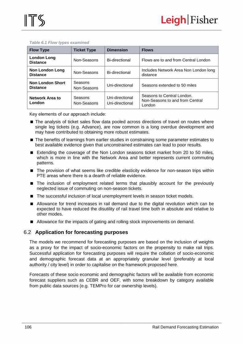
106 Rail Demand Forecasting Estimation
Table 6.1 Flow types examined
Flow Type Ticket Type Dimension Flows
London Long Distance
Non-Seasons Bi-directional Flows are to and from Central London
Non London Long Distance
Non-Seasons Bi-directional Includes Network Area Non London long distance
Non London Short Distance
Seasons
Non-Seasons Uni-directional Seasons extended to 50 miles
Network Area to London
Seasons
Non-Seasons
Uni-directional
Uni-directional
Seasons to Central London. Non-Seasons to and from Central London
Key elements of our approach include:
The analysis of ticket sales flow data pooled across directions of travel on routes where single leg tickets (e.g. Advance), are now common is a long overdue development and may have contributed to obtaining more robust estimates.
The benefits of learnings from earlier studies in constraining some parameter estimates to best available evidence given that unconstrained estimates can lead to poor results.
Extending the coverage of the Non London seasons ticket market from 20 to 50 miles, which is more in line with the Network Area and better represents current commuting patterns.
The provision of what seems like credible elasticity evidence for non-season trips within PTE areas where there is a dearth of reliable evidence.
The inclusion of employment related terms that plausibly account for the previously neglected issue of commuting on non-season tickets.
The successful inclusion of local unemployment levels in season ticket models.
Allowance for trend increases in rail demand due to the digital revolution which can be expected to have reduced the disutility of rail travel time both in absolute and relative to other modes.
Allowance for the impacts of gating and rolling stock improvements on demand.
6.2 Application for forecasting purposes
The models we recommend for forecasting purposes are based on the inclusion of weights
as a proxy for the impact of socio-economic factors on the propensity to make rail trips.
Successful application for forecasting purposes will require the collation of socio-economic
and demographic forecast data at an appropriately granular level (preferably at local
authority / city level) in order to capitalise on the framework proposed here.
Forecasts of these socio economic and demographic factors will be available from economic
forecast suppliers such as CEBR and OEF, with some breakdown by category available
from public data sources (e.g. TEMPro for car ownership levels).

Final Report 107
6.3 Recommended elasticities and recommendations for forecasting
As they are outside the scope of this study, which is intended to review exogenous factors,
we do not make recommendations about the effects of fares, GJT, or any other factors
endogenous to the rail industry (except as described in section 6.3.6 below).
We understand that a separate study on fares elasticities has been undergoing at the same
time as this study. We would expect its recommendations to be used in future forecasting.
As a proxy for those recommendations, we estimated fares elasticities (using yield deflated
by CPI) in our modelling and applied these estimates in our backcasts; the backcast results
compared to current WebTAG recommendations (PDFH 4.0 and an RPI deflator).
Our modelling did not extend to seasons within PTE areas, season flows from London to the
Network Area and seasons flows between London and the ‘Rest of Country’.
The first of these segments was excluded because we do not have data covering the sales
and usage of PTE zonal tickets. Our models covered non-PTE and non-London flows; these
cover commuting into metropolitan cities from outside the metropolitan areas as well as rail
commuting into non-metropolitan cities (many of which also have significant numbers of rail
commuters). We would recommend using the elasticities and recommendations for flows
into PTE areas. As discussed in sections 4.7 and 6.5, non-London rail commuting is a key
opportunity for further research.
Season volumes ‘from’ London ‘to’ the Network Area (although seasons are always priced
identically and so origin-destination of the ticket may not reflect production-attraction of the
passenger) have grown at a slightly slower rate than flows in the opposite ‘direction’. We
would recommend using the elasticities and recommendations derived from flows in the
other direction, reflecting the likely similarity in the markets. The components of the
socioeconomic indices have been derived combining trips to and from London.
The number of season ticket travellers from stations outside the Network Area to London is
significantly smaller than from within the Network Area (about 4% of the size); the dominant
origins (non-London stations) are one or two stops outside of the Network Area. We
recommend using the same elasticities and recommendations as for Network Area to
London flows.
Socioeconomic Characteristics (POP_INDEXSE and EMP_INDEXSE) 6.3.1
We have constructed a new index for producing the weighted population and employment
measure. The trip rate (index) is calculated by taking the base figure (the first row in the
table below) and adding the product of each of the subsequent numbers by the share of the
population (employees where applicable) that belong to that category. This index will change
over time.
In our modelling we have multiplied this index by the total population at the origin (or
employment at the destination). In principle, though, it would be perfectly possible to include
the (change in) the two terms separately in the demand forecast, with the appropriate
elasticity to both.

108 Rail Demand Forecasting Estimation
For the weighted population measure ‘POP_INDEXSE’, calculate the index for ‘other’ trips
and then add the index for ‘employer’s business trips’ multiplied by the share of the
population who are employed.
For the weighted employment measure ‘EMP_INDEXSE’, calculate the index for ‘commute
trips’.

Final Report 109
Population Measures
Table 6.2 Recommended values for population socioeconomic index
Non-London To/from London
‘Other’ Employer’s Business
‘Other’ Employer’s Business
Base Trip Rate 0.0618 0.0119 0.0267 0.0206
Share of population aged
0-14 -0.0079 -0.0127
15-29 0.0494 -0.0023 0.011 -0.008
30-44 -0.0023 0.0015 0.0092 0.0044
45-64 -0.019 0.0001 -0.001 0.0012
65+ -0.017 -0.0023 -0.0097 -0.0046
Share of employed population employed as/in
managers, directors and senior officials
-0.0186 0.0119 0.0181 0.0303
professional occupations 0.0155 0.0147 0.0314 0.0301
associate professional and technical occupations
0.0073 0.0100 0.025 0.0148
administrative and secretarial occupations
0.0038 -0.0064 0.0041 -0.0151
skilled trades occupations -0.0233 -0.0071 -0.0132 -0.0132
caring, leisure and other service occupations
-0.0017 -0.0065 -0.0054 -0.0164
sales and customer service occupations
0.0226 -0.0076 -0.0075 -0.0172
process, plant and machine operatives
-0.0255 -0.0071 -0.02 -0.0134
elementary occupations 0.0062 -0.0067 -0.0065 -0.0156
Share of employed population employed in
manufacturing -0.0167 -0.0079 -0.0114 -0.0033
construction -0.0173 -0.0080 -0.0069 -0.011
wholesale, retail & repair of motor vehicles, accommodation
-0.0021 -0.0055 -0.009 -0.0143
finance or insurance; real estate; professional, scientific or technical activities; administrative or support services
0.0008 0.0105 0.0211 0.0268
public admin or defence; social security; education; human health; social work
-0.0027 0.0007 0.0042 -0.0059
Other services 0.005 0.0015 0 0.0029
Share of population living in a household with
No car 0.0223 0.0019 0.0024 -0.0024
1 car 0.0005 0.0001 -0.0002 -0.0018
2 cars -0.0098 -0.0004 0.0006 0.0020
3 or more cars -0.0144 -0.0009 -0.0045 0.0016

110 Rail Demand Forecasting Estimation
Employment Measures (Commute Trip Rates)
Table 6.3 Recommended values for employment socio-economic index
Non-London To London
Base Trip Rate 0.0879 0.079
Share of population at origin aged
15-29 0.042 -0.0121
30-44 0.0038 0.0193
45-64 -0.027 -0.0085
65+ -0.0593 -0.0456
Share of jobs at destination working as/in
managers, directors and senior officials 0.0312 0.0836
professional occupations 0.0483 0.0854
associate professional and technical occupations
0.0413 0.042
administrative and secretarial occupations
0.0582 0.0055
skilled trades occupations -0.0504 -0.0505
caring, leisure and other service occupations
-0.0434 -0.0579
sales and customer service occupations
-0.0327 -0.0606
process, plant and machine operatives -0.0468 -0.0499
elementary occupations -0.0326 -0.0548
Share of jobs at destination working in
manufacturing -0.0426 -0.0394
construction -0.0284 -0.021
wholesale, retail & repair of motor vehicles, accommodation
-0.0206 -0.0535
finance or insurance; real estate; professional, scientific or technical activities; administrative or support services
0.077 0.1205
public admin or defence; social security; education; human health; social work
-0.0022 -0.0134
Other services 0.0043 0.0048
Share of population at origin living in a household with
No car 0.0945 0.0098
1 car 0.0223 0.0041
2 cars -0.0241 0.0022
3 or more cars -0.0388 -0.0181
In our non-season (‘ordinary’) ticket models, we have included employment and population
(i.e. commute and non-commute) measures separately, related to the appropriate variable,
except for long distance flows where we assume commuting is negligible. When we
constructed models without employment in, we used a different POPSE measure that
included the commute trip rates, multiplied (reduced) by the share of population in a job and
the share of commute journeys that are on ordinary tickets.
We do not make any allowance for increasing non-commute trip rates in the models for
season tickets, as changes in non-commute trip rates seem unlikely to influence season
ticket purchases.

Final Report 111
Population and employment elasticities 6.3.2
These recommendations come from our preferred models, with employment elasticities
rounded to the nearest 0.05.
The participation rate is defined as the share of the population at the origin (production end)
aged 15-64 who are employed (this is the same, but with opposite sign, as the
unemployment rate used in the ticket sales models, as described in section 5.1). This is a
slightly different measure from that used in constructing the socioeconomic indices.
The negative sign implies that reduced participation at the origin (presumably reflecting the
availability of jobs near home) is associated with a relatively small increase in rail commuting
to the destination (given the number of jobs there). The participation rate effect should be
applied as a semi-elasticity, i.e. the demand function is of the form:
𝐷𝑒𝑚𝑎𝑛𝑑 = ⋯ × 𝑃𝑂𝑃_𝐼𝑁𝐷𝐸𝑋𝑆𝐸𝐸𝑙𝑎𝑠𝑡𝑖𝑐𝑖𝑡𝑦 × 𝐸𝑀𝑃_𝐼𝑁𝐷𝐸𝑋𝑆𝐸
𝐸𝑙𝑎𝑠𝑡𝑖𝑐𝑖𝑡𝑦 × 𝑒𝑃𝑎𝑟𝑡𝑅𝑎𝑡𝑒 × 𝑆𝑒𝑚𝑖−𝐸𝑙𝑎𝑠𝑡 × …
We have used a ‘workplace’ measure of employment (i.e. the number of jobs) at the
destination (attraction) end to quantify our employment elasticities. The participation rate
uses a ‘residential’ measure of employment (i.e. the number of workers living there) at the
origin (production) end to quantify the participation rate semi-elasticities.
Table 6.4 Recommended population and employment elasticities
Ticket type
Flow Population (POP_INDEXSE) elasticity
Employment (EMP_INDEXSE) elasticity
Participation rate semi-elasticity
Ordinary Rest of Country to/from London 1 0 0
Ordinary Network Area to/from London 1 0.2 0
Ordinary Non-London, >20 miles 1 0 0
Ordinary Non-London, PTE areas, <20 miles
1 0.25 0
Ordinary Non-London, non-PTE, <20 miles 1 0.1 0
Season To/from London 0 1 −0.18
Season Non-London, non-Core, < 20 miles
0 1 −0.23
Season Non-London, to/from core, < 20 miles
0 2.5 −0.23
Season Non-London, non-Core, > 20 miles
0 1.2 −0.23
Season Non-London, to/from core, > 20 miles
0 2.7 −0.23
For non-London seasons, these employment index elasticities are larger than one; this
implies rail capturing an increasing share of commuters as the number of jobs grows, above
the changing share associated with the socioeconomic index described in section 6.3.1 as
the types of jobs (occupations and sectors) change.

112 Rail Demand Forecasting Estimation
Income elasticities 6.3.3
These recommendations come from our preferred models, rounded to the nearest 0.05. In
our models we measured income using GVA per capita at the origin, as this produced a
better model fit than Gross Disposable Household Income.
Table 6.5 Recommended income elasticities
Ticket type Flow Income elasticity
Ordinary Rest of Country to/from London 0.7
Ordinary Network Area to London 1.05
Ordinary Network Area from London 1.05
Ordinary Non-London, >20 miles, between core cities 1.25
Ordinary Non-London, >20 miles, other flows 1.0
Ordinary Non-London, PTE areas, <20 miles, to or from core city or major centre 0.9
Ordinary Non-London, PTE areas, <20 miles, other flows 0.7
Ordinary Non-London, non-PTE, <20 miles, to or from core city or major centre 1.1
Ordinary Non-London, non-PTE, <20 miles, other flows 0.9
Season To/from London 0.5
Season Non-London 0
We did not consider that we had identified robust estimates of an income effect for non-
London seasons. Note that the preferred model for Network Area Ordinary ticket flows was
suggesting an income elasticity of only 0.2 on from London flows (versus 1.05 on to London
flows). Whilst this can be rationalised when considering differential historic GVA growth rates
we recommend that the to London value be used on all London flows, regardless of
direction.
Car competition 6.3.4
These recommendations come from a combination of section 3.4 (where we reviewed
previous evidence) and the purpose splits estimated by this project and included in Annex C.
They are very similar to existing WebTAG recommendations (from PDFH 5.0), albeit using
different purpose splits.
We do not include a separate term for non-car ownership, which is included as part of
section 7.3.1 above. These imply weaker effects than currently assumed by PDFH.

Final Report 113
Table 6.6 Recommended effects of car competition
Ticket type Flow Car cost cross-elasticity
Car time cross-elasticity
Ordinary Rest of Country to/from London 0.21 0.28
Ordinary Network Area to/from London 0.19 0.22
Ordinary Non-London <20 miles 0.4 0.2
Ordinary Non-London > 20 miles 0.26 0.3
Season To/from London 0 0
Season Non-London 0.4 0.2
Bus and coach competition 6.3.5
We have not included the effects of bus and coach competition in our modelling. This is due
to the absence of robust historical data to quantify changes in bus and coach competition,
not because we think that they should be included in rail demand forecasts. We have
reviewed the existing recommendations and proposed reducing the cross-elasticities
currently recommended by PDFH, as discussed below.
The effects recommended by PDFH date back to reviews of modal choice models, cited in
the National Passenger Demand Forecasting Framework. That report dates back to 1999,
and since then rail demand has grown significantly whereas (outside London) bus and coach
demand has fallen. Table 6.7 repeats results from NTS data:
Table 6.7 Miles per person per year for selected modes. Source: DfT statistics table NTS0305
Miles per person per year
Mode 1995/97 2014 Change
Surface rail 341 540 +58%
Other [Non-London] local bus 203 199 -2%
Non-local bus 94 50 -47%
All non-London bus 297 249 -16%
The declining use of ‘non-local buses’, i.e. coaches, is particularly striking. PDFH provides a
formula that gives a derivation for cross-elasticities:
Assuming the diversion factor and own-price elasticity of bus (and coach) travel has not
changed, the impact of the change in relative shares will have been to reduce the cross-
price elasticity. The intuition is that if the number of bus passengers has declined and a fixed
share of them is lost to rail for each (proportionate) change in price (or journey time or
headway), then the (proportionate) impact of this on the level of rail demand will have
declined too.

114 Rail Demand Forecasting Estimation
Table 6.8 Shares of bus and coach relative to rail
Relative Share 1995/97 2014 Change
Non-London local bus passenger miles per (National) surface rail passenger mile
0.60 0.37 -38%
Non-local bus (i.e. coach) passenger miles per (National) surface rail passenger mile
0.28 0.09 -66%
Thus, for bus we reduce the cross-elasticity for each journey purpose by 40% and for coach
by two-thirds.
We recommend using the factors recommended by NPDFF but updated to reflect our NTS-
derived understanding of journey purposes (Annex C) and reduced to reflect the change in
‘relative shares’. The NPDFF recommendations are shown in Table 6.9 below:
Table 6.9 NPDFF recommended cross-elasticities for bus and coach
Segment Purpose Cost Journey time
Headway
Non-London Urban (bus)
Commute
Business
Leisure
Inter-Urban (coach)
Commute *
Business *
Leisure to/from London *
Leisure non-London *
Network Area inc. to/from London (coach)
Commute to London *
Commute non-London *
Business *
Leisure *
* NPDFF does not include recommendations for coach headway. In PDFH (4.0 et seq.) it appears to have been assumed that the cross-elasticity is the same as for buses.
It is not immediately apparent why short (i.e. bus) trips should be different within and outwith
the Network Area, nor why commuters would use coaches to London when they are
travelling from outside the Network Area. Adjusting for the change in relative shares since
NPDFF, our recommendations by journey purpose are thus shown below:

Final Report 115
Table 6.10 RDFE Recommended cross-elasticities by purpose
Segment Purpose Cost Journey time
Headway
Bus (inc. Network Area)
Commute
Business
Leisure
Coach to/from London
Commute
Business
Leisure
Coach non-London
Commute
Business
Leisure
And mapped to ticket types:
Table 6.11 Recommended bus/coach cross-elasticities by ticket type
Ticket type
Flow Mode Cost Journey time
Headway
Ordinary Rest of Country to/from London
Coach 0.06 0.06 0.01
Ordinary Network Area to/from London
Coach 0.06 0.06 0.01
Ordinary Non-London <20 miles Bus 0.16 0.06 0.03
Ordinary Non-London > 20 miles Coach 0.06 0.06 0.01
Season To/from London Coach 0 0 0
Season Non-London <20 miles Bus 0.12 0.06 0.03
Season Non-London > 20 miles Coach 0.07 0.07 0.02
We considered that these are typical values, and suitable for application where no other
information on the extent of competition is available. On specific flows they are likely to vary
significantly with rail’s competitive position. For most commuter flows to/from London, coach
competition is virtually absent. There are some flows where commuter coaches still operate,
notably in Hertfordshire and North Kent. In such cases, appropriate cross-elasticities (taking
into account the market size) should be used.
Terms outside of the framework 6.3.6
In our preferred models we have included a term, ‘GJT_Trend’, which allows for other drivers
of rail demand, such as improvements in mobile communications that have made rail travel
more productive and more pleasant. This has been quantified by reducing GJT by 1% per
year from 2000/01. This can be implemented as an index valued at 1 for each year through
1999/2000 and then reducing to 0.86 in 2013/14, raised to the GJT elasticity.
This gives -% more demand (depending on the GJT elasticity) over the fifteen years for
which it applies. As can be seen in section 4 (the differences between models I and III) the
main effect of including this term is to reduce the income elasticity. Not making an allowance
for this component of market growth would overstate the impact of changes in income
(growth) on levels of rail travel. However, rolling forward the same trend for all future years

116 Rail Demand Forecasting Estimation
would assume that the technological developments favourable to rail travel would continue
at the same pace into the future.
In a forecast of rail demand (and/or revenue) into the future, one should assess the impact of
all factors that would cause demand growth – changes in crowding, marketing, yield
management, rolling stock quality, station facilities and indeed mobile connectivity. In some
contexts, there will be uncertainty over the future change in these factors. Some allowance
may need to be made for other factors contributing to growing rail demand: this should be
considered carefully.
6.4 Recommendations for Data Collection
Rail Usage and Demand Drivers 6.4.1
RUDD is a useful dataset for rail demand and drivers data; maintaining and updating it will
allow further projects like ours to review past experience to improve future demand forecasts.
However, we make the following recommendations for its improvement:
Combine the London BR and Zone R1 London groups, at least for flows outside the Travelcard area. It is not obvious why they should be considered separate flows for demand purposes.
Adjust the exogenous data for London BR (and Zone R1 London) to reflect Central London as a whole, not just Westminster.
Review the employment data to provide the best possible time series, with suitable caveats for methodological (e.g. LFS to APS) breaks. This is what we have attempted to do for this study.
Review the purpose of the AML data – it will be difficult to provide a continuous time series as the definition of service codes and groups change over time. What appears to be the current method (weighted averages over service codes) exacerbates this problem; using the data for the single most important service code/group for a flow would be a sensible alternative.
Consider adding data on ‘endogenous’ initiatives. The gating of each station would be an obvious additional data item and is fairly well-defined, although would require each flow to have (at least) an identified origin/destination station where it is currently a group and for historical data to be collated. The typical fleet (e.g. the most frequently occurring rolling stock type on the most important service code) and the levels of crowding (e.g. PiXC for the TOC or service group) may also be worthwhile additions.
Separate the station-year data (e.g. employment for London BR in 2016) from the flow-year data (e.g. number of standard class reduced trips from Cambridge to Leeds in 2016) to make the data files more manageable, with no loss of content.
NTS data 6.4.2
A wide variety of data are collected in NTS and we have used only a very small proportion
(that relating to rail trips and passengers) in this study. However, it might be possible to
improve the collection of data relating to ticket types by matching the terms used in the travel
diary with the terms printed on tickets.
Currently, respondents are told:

Final Report 117
“Write here the type of ticket used. Tell us if it was a single, a return, a season ticket or
a one day travelcard. If you were able to buy a ticket at a cheap rate please write this
in too. If you used reduced or free tickets, or a concessionary pass that allows you to
travel for free, please tell us. If you used an Oyster card please tell us whether it was a
pre-pay or a season ticket.”
This instruction applies for both buses and rail. We are not aware of how these data are
used for buses. In rail, we observed a significant under-reporting of full (anytime) relative to
reduced (off-peak or advance) tickets when comparing NTS and ticket sales data; to some
degree this may be unavoidable, because we would not necessarily expect people to have
retained their ticket when completing the diary. However, using the same words that appear
on the tickets – the terms ‘cheap rate’ and ‘reduced’ have technical meanings but would not
necessarily be familiar to passengers; some reduced tickets are priced highly or valid almost
all day and so might be perceived full fare. It may not be necessary to enquire as to whether
the ticket was a single or a return. An alternative wording could be:
“Write here the type of ticket used. For buses, tell us if it was a single ticket, a return
ticket, an all-day ticket or a ticket valid for a week or more. For trains, tell us if it was an
anytime, off-peak, advance or season ticket. If you used a concessionary pass that
allows you to travel for free, please tell us. If you used an Oyster card please tell us
whether it was a pre-pay or a season ticket.”
This would improve the use of NTS data in understanding the trip purposes of travellers on
each ticket type. This would allow estimates made using the approach in Annex B to be
improved in future.
As has regularly been found in the analysis of NTS data, the geographical limitations of the
data available to analysts limits the accuracy of their work. For example, the coding of a
destination as ‘Cambridgeshire’ does not permit the testing of city effects, such as parking
restrictions or types of employment that may be very relevant to rail demand. Any
improvement that allowed more accurate analysis would be welcome. Possibly the area type
indicators could also be used to obtain further insights.
6.5 Recommendations for Implementing the Forecasting Framework
Implementing the recommended forecasting framework will make rail forecasting more
complicated than the traditional Passenger Demand Forecasting Handbook approach. This
is because this methodology adds in an extra step of calculating the INDEXSE variables
before the elasticity calculation is done. This extra complexity makes it essential that robust
Quality Assurance and review processes are put in place. The Department for Transport has
published some guidance on Analytical Assurance and Quality Assurance which may be of
interest1.
1 https://www.gov.uk/government/publications/dft-analytical-assurance-framework-strength-in-numbers

118 Rail Demand Forecasting Estimation
6.6 Recommendations for Further Research
Using NTS data
Regarding the NTS data, we have identified potential extensions to the disaggregate
modelling, which would improve the level of explanation achieved, and extend the modelling
including new or improved variables. It is likely that this work could be done for moderate
additional budget (unless destination and mode choice effects were to be included) and
could yield important new insights.
Non-London Commuting
Our socio-economic adjustments to the employment estimates, which uses the evidence
from NTS to allow for the impact of ‘structural change’ where jobs in cities have been
increasingly oriented towards sectors which are more favourable to rail travel, has made an
important step. However, as discussed in sections 4.7 and 5.5, the performance of models of
non-London season demand is relatively poor. We considered models including an income
elasticity, but the estimated income elasticity was implausibly high (higher than for non-
season tickets); further, such an elasticity does not explain the continuing strong growth in
season patronage in recent years when income growth has been weak or negative.
We have identified substantial differences between cities in the growth in employment (both
with and without our socioeconomic adjustments) and the growth in season passenger
volumes; in recent years cities with similar growth in employment have experienced very
different levels of growth in season ticket patronage. An improved method of forecasting
growth in commuting outside London should begin to explain the differences between cities.
Data collection is likely to be the greatest challenge. This may involve collating better data
on employment near stations – we used employment numbers for the district, which is
broadly consistent with our use of the NTS data, where we use levels of rail trip making for
the entire population given age, sector etc. It might be the case that certain age groups are
likely to live near stations, or certain sectors’ offices are likely to be located near stations. In
any case, the data on employment within 1km of stations (available for only part of the time
period) already included in RUDD did not show greater levels of growth.
Data collection may also involve collecting data on the competitive circumstances around
individual routes, such as the relative availability and price of car parking between different
cities.
Differences between full and reduced markets
As part of phase one, we reviewed the split of passenger volume by ticket type for each of
the market segments and observed how it changes over time. On longer distance flows
there has been a significant increase in the share of passengers travelling on advance
tickets over the past twenty years; in more recent years, this has been at the expense of the
full ticket market as well as the reduced ticket market. In the shorter distance market, in the
Network South East area there was a marked increase in the share of full tickets at the
expense of reduced between 1999 and 2005, and a decline in the sale of reduced tickets for
non-London flows subsequently.

Final Report 119
We consider it most likely that this was because of changes in ticket restrictions. This would
mean that the underlying composition of the full and reduced markets will have changed
over time; further, estimating a model for full fare tickets (for instance) that neglected the
influence of increased restrictions on reduced tickets and/or increased availability of advance
tickets would result in inappropriate estimates of income elasticities and/or other effects.
It seems likely that the reduced ticket market would be more sensitive to income than the full
ticket market, because of the greater presence of commuting trips on full price tickets.
However, work to estimate separate income elasticities would require on appropriate
measures of ticket restrictions allowing for such changes to be controlled for.
Advance tickets, and active yield management policies, may well capture those portions of
the market that are most price-sensitive. However, the large growth in advance ticket sales
is more likely to reflect increasing availability of these products – now, advance tickets are
available at much shorter notice and on almost any train, with the prices having changed to
reflect this. Modelling the different components of the long distance market using ticket sales
data would almost certainly need to rely upon distinguishing on the purposes of travellers’
trips (such as by using CRM data from ticket sales systems), the time of day on which they
are travelling (using data on the trains they chose, for advance tickets at least) or the
duration of trips (again using ticket sales systems to ‘match’ single leg tickets). Such work
would prove fruitful in understanding the future growth in different components of the travel
market and ensuring future service provision reflects this.
Airline competition
RUDD includes data on ‘competing’ airline flows. Station-stations pairs (rail flows) are
matched with airport-airport pairs (air flows) and there are data on prices, service levels and
passenger volumes. There are two important limitations with these data:
For some flows – notably long distance travel to/from London – the compared data is a single airport pair, whereas multiple airport pairs may be competing with rail (e.g. the Glasgow BR – London BR flow is mapped to Glasgow Airport – Heathrow, whereas service levels at London City, Luton and Stansted may also be relevant); and
The convenience of the airports for a specific flow, especially non-London flows, will differ drastically: Newcastle – Birmingham may be the best airport for both flows, but competition with rail is likely to be stiffer for the Newcastle – Coventry market than the Carlisle – Birmingham market.
Nevertheless, fruitful analysis may well be possible. This would probably need to consider a
much more limited set of flows than we have here, and take into account multiple airport
pairs for each rail flow. Customers with different trip purposes (and paying different fares)
may have different propensities to switch between air and rail. A suitable method for
modelling air competition may give better estimates of income elasticities for longer distance
London markets, where we have observed weak growth in recent times.
Rolling stock
It is disappointing that our aggregate data was not able to estimate effects of changes in
rolling stock that were of plausible size. This may reflect the omission of crowding data, as
changes in the composition of a rolling stock fleet are often linked with changes in the size of
that fleet: implausibly large estimated effects of rolling stock may be connected with

120 Rail Demand Forecasting Estimation
significant crowding relief. Future analysis of the impacts of rolling stock should take this into
account. Large aggregate data sets like RUDD should be useful in providing convincing
estimates of the effect of fleet changes.
Dynamics
Our models are entirely static ones – changes in rail demand drivers are assumed to have
their effects felt in full instantly. This partly reflects our use of annual data, though estimates
of (say) local population covering shorter periods are unlikely to be precise or timely enough
to forecast (say) periodic changes in rail demand. However, especially inasmuch as changes
in rail demand are at the extensive margin (analogous to the stop/go component of the NTS
models) rather than the intensive margin, habits take time to form and so changes in rail
demand may be observed over longer periods of time. Our intuition is that for exogenous
factors dynamic effects are unlikely to be important. Nevertheless, further work could identify
the timing of effects and, if the lags are significant, result in different estimates from this
report.
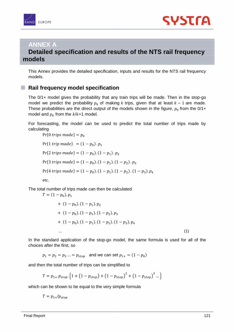
Final Report 121
ANNEX A Detailed specification and results of the NTS rail frequency models
This Annex provides the detailed specification, inputs and results for the NTS rail frequency
models.
Rail frequency model specification
The 0/1+ model gives the probability that any train trips will be made. Then in the stop-go
model we predict the probability 𝑝𝑘 of making 𝑘 trips, given that at least 𝑘 − 1 are made.
These probabilities are the direct output of the models shown in the figure, 𝑝0 from the 0/1+
model and 𝑝𝑘 from the 𝑘/𝑘+1 model.
For forecasting, the model can be used to predict the total number of trips made by
calculating
Pr{0 𝑡𝑟𝑖𝑝𝑠 𝑚𝑎𝑑𝑒} = 𝑝0
Pr{1 𝑡𝑟𝑖𝑝 𝑚𝑎𝑑𝑒} = (1 − 𝑝0) . 𝑝1
Pr{2 𝑡𝑟𝑖𝑝𝑠 𝑚𝑎𝑑𝑒} = (1 − 𝑝0). (1 − 𝑝1) . 𝑝2
Pr{3 𝑡𝑟𝑖𝑝𝑠 𝑚𝑎𝑑𝑒} = (1 − 𝑝0). (1 − 𝑝1). (1 − 𝑝2) . 𝑝3
Pr{4 𝑡𝑟𝑖𝑝𝑠 𝑚𝑎𝑑𝑒} = (1 − 𝑝0). (1 − 𝑝1). (1 − 𝑝2) . (1 − 𝑝3). 𝑝4
etc.
The total number of trips made can then be calculated
𝑇 = (1 − 𝑝0). 𝑝1
+ (1 − 𝑝0). (1 − 𝑝1). 𝑝2
+ (1 − 𝑝0). (1 − 𝑝1). (1 − 𝑝2). 𝑝3
+ (1 − 𝑝0). (1 − 𝑝1). (1 − 𝑝2). (1 − 𝑝3). 𝑝4
... (1)
In the standard application of the stop-go model, the same formula is used for all of the
choices after the first, so
𝑝1 = 𝑝2 = 𝑝3 … = 𝑝𝑠𝑡𝑜𝑝 and we can set 𝑝1+ = (1 − 𝑝0)
and then the total number of trips can be simplified to
𝑇 = 𝑝1+.𝑝𝑠𝑡𝑜𝑝. {1 + (1 − 𝑝𝑠𝑡𝑜𝑝) + (1 − 𝑝𝑠𝑡𝑜𝑝)2
+ (1 − 𝑝𝑠𝑡𝑜𝑝)3
… }
which can be shown to be equal to the very simple formula
𝑇 = 𝑝1+/𝑝𝑠𝑡𝑜𝑝

122 Rail Demand Forecasting Estimation
In the present application, however, we need to allow for variations of probability at different
points in the choice process, so that we need to use the form in equation (1).
The models used are binary logit models, that is, they represent choice by
𝑃(0) =exp(𝑉0)
1+exp(𝑉0) and 𝑃(𝑘) =
exp(𝑉𝑘)
1+exp(𝑉𝑘)
where 𝑉0 is the utility of making zero trips, relative to the utility of making 1 or more;
𝑉𝑘 is the utility of making exactly 𝑘 trips, relative to the utility of making 𝑘 + 1 or more.
The specification of the model is then a matter of specifying the utility functions used in these
formulae. 𝑉0 is always specified separately for a given travel purpose, but we specify 𝑉𝑘 to
be a standard formulation for the purpose with a possible additional component for making
exactly 𝑘 trips, i.e.
𝑉𝑘 = 𝑉𝑠𝑡𝑜𝑝 + 𝛿𝑘
where 𝛿𝑘 is a ‘dummy’ variable specific to the choice of k trips and
𝑉𝑠𝑡𝑜𝑝 is otherwise standard for all numbers of trips for each purpose.
Utility terms appearing in 𝑉0 then point to the probability that a given individual will use train
at all during the week, whereas terms in 𝑉𝑠𝑡𝑜𝑝 point to the probability that multiple trips will be
made. Note that terms are always attached to the alternative of making fewer trips, i.e.
negative terms imply more train travel, and positive terms imply less train travel; these signs
are reversed in the presentation in the main text to make it more intuitive.
NTS data definitions
Below we summarise the key socio-economic variables contained in the NTS data and their
definitions.

Final Report 123
Table A.2 NTS variable definitions
NTS Variable Definition
NTS Purpose (TripPurpose_B04ID)
Commuting
Business
Other purposes include:
Education/Escort education
Shopping
Other Escort
Personal Business
Leisure
Other just including walk
Age Continuous variable
NumCarVan (Number of household cars or light vans (including landrover, jeep, minibus etc) - actual number)
Continuous variable
Ethnicity (15 groups)
White British
Other white background
White and Black Caribbean
White and Black African
White and Asian
Any other mixed background
Indian
Pakistani
Bangladeshi
Any other Asian background
Caribbean
African
Any other black background
Chinese
Any other

124 Rail Demand Forecasting Estimation
NTS Variable Definition
Income (Banded household and personal incomes available; extended from 21 to 23 bands in 2002)
Less than £1000
£1000 - £1999
£2000 - £2999
£3000 - £3999
£4000 - £4999
£5000 - £5999
£6000 - £6999
£7000 - £7999
£8000 - £8999
£9000 - £9999
£10000 - £12499
£12500 - £14499
£15000 - £17499
£17500 - £19999
£20000 - £24999
£25000 - £29999
£30000 - £34999
£35000 - £39999
£40000 - £49999
£50000 - £59999
£60000 - £69999
£70000 - £74999
£75,000+
Italicised bands available 2002 onwards only
Economic status
Employees: full-time
Employees: part-time
Self-employed: full-time
Self-employed: part-time
ILO unemployed
Economically inactive: Retired
Economically inactive: Student
Economically inactive: Looking after family/home
Economically inactive: Permanently sick/disabled
Economically inactive: Temporarily sick/injured
Economically inactive: Other
Occupation (SOC classification)
Managers and senior officials
Professional occupations
Associate professional and technical occupations
Administrative and secretarial occupations
Skilled trades occupations
Personal service occupations
Sales and customer service occupations
Process, plant and machine operatives
Elementary occupations

Final Report 125
NTS Variable Definition
Standard Industrial classification (SIC 1992 bandings)
A - Agriculture, hunting and forestry
B – Fishing
C - Mining and quarrying
D – Manufacturing
E - Electricity, gas and water supply
F – Construction
G - Wholesale and retail trade
H - Hotels and restaurants
I - Transport, storage and communication
J - Financial intermediation
K - Real estate, renting and business activities
L - Public administration and defence; compulsory social security
M – Education
N - Health and social work
O - Other community, social and personal service activities
P - Private households with employed persons
Q - Extra-territorial organisations and bodies
Rail ticket type (stage variable)
Ordinary adult
Ordinary child
Reduced ordinary adult
Reduced ordinary child
Special category reduced
Other (including free)
Season ticket
Travel card
Combined season/travel card
Railcard
Concessionary - Employees
Other non concessionary
OAP pass
Scholars pass
Disabled persons pass
Subsidised travel tokens
Other concessionary
NTS sample distribution by age, gender and working status
The following tables show the distribution of unweighted population in NTS database (1995-
2014) for each year by gender, age, working status and occupation.

126 Rail Demand Forecasting Estimation
Table A.3 NTS sample sizes by gender
Number of individuals Percentage
Year Male Female Total Male Female
1995 4,239 4,661 8,900 47.6% 52.4%
1996 4,105 4,341 8,446 48.6% 51.4%
1997 4,072 4,376 8,448 48.2% 51.8%
1998 3,862 4,101 7,963 48.5% 51.5%
1999 3,814 4,168 7,982 47.8% 52.2%
2000 4,268 4,640 8,908 47.9% 52.1%
2001 4,212 4,641 8,853 47.6% 52.4%
2002 10,019 10,808 20,827 48.1% 51.9%
2003 10,652 11,338 21,990 48.4% 51.6%
2004 10,378 11,210 21,588 48.1% 51.9%
2005 10,938 11,764 22,702 48.2% 51.8%
2006 10,699 11,442 22,141 48.3% 51.7%
2007 10,551 11,380 21,931 48.1% 51.9%
2008 10,259 10,906 21,165 48.5% 51.5%
2009 10,541 11,294 21,835 48.3% 51.7%
2010 10,109 10,730 20,839 48.5% 51.5%
2011 9,631 10,357 19,988 48.2% 51.8%
2012 10,253 10,990 21,243 48.3% 51.7%
2013 9,160 9,605 18,765 48.8% 51.2%
2014 8,670 9,239 17,909 48.4% 51.6%
Total 160,432 171,991 332,423 48.3% 51.7%
Table A.4 Proportion of NTS sample by age band
Year 0-4 5-10 11-16 17-20 21-29 30-39 40-49 50-59 >60 Total
1995 7% 9% 8% 4% 12% 15% 14% 11% 19% 100% 1996 7% 8% 8% 5% 11% 15% 15% 11% 21% 100% 1997 7% 9% 8% 4% 11% 15% 13% 12% 19% 100% 1998 7% 8% 8% 5% 12% 15% 13% 12% 20% 100% 1999 6% 8% 8% 4% 11% 15% 14% 13% 21% 100% 2000 7% 8% 8% 5% 10% 15% 14% 12% 21% 100% 2001 6% 8% 8% 4% 10% 15% 13% 13% 22% 100% 2002 6% 8% 8% 4% 10% 15% 14% 13% 22% 100% 2003 6% 8% 8% 4% 10% 15% 14% 13% 21% 100% 2004 6% 8% 9% 4% 10% 14% 14% 13% 22% 100% 2005 6% 8% 8% 5% 10% 14% 15% 13% 22% 100% 2006 6% 8% 8% 5% 10% 13% 15% 13% 22% 100% 2007 6% 7% 8% 4% 10% 13% 15% 13% 23% 100% 2008 6% 7% 8% 5% 10% 13% 15% 12% 24% 100% 2009 7% 7% 8% 5% 10% 13% 14% 13% 24% 100% 2010 6% 7% 8% 5% 9% 12% 15% 12% 25% 100% 2011 6% 7% 7% 5% 10% 12% 14% 13% 25% 100% 2012 7% 7% 7% 5% 10% 12% 14% 13% 25% 100% 2013 7% 8% 7% 4% 11% 12% 14% 12% 25% 100% 2014 7% 8% 8% 4% 10% 13% 14% 13% 25% 100%
Total 6% 8% 8% 5% 10% 13% 14% 13% 23% 100%

Final Report 127
Table A.5 Fraction of NTS sample by working status
NTS rail frequency model results
The following tables summarise the model results (including both ‘none’ and ‘stop-go’ stages)
for each purpose and geography. Two sets of values are presented:
model summary statistics
model coefficient values and their associated t-ratios.
We present both the final model results, where insignificant and coefficients with
counterintuitive signs have been merged with other categories or constrained to zero, and
the models with all coefficients are freely estimated (unconstrained). In the unconstrained
models, insignificant coefficients that have been constrained to zero or merged are
highlighted in red. We also highlight the counterintuitive company car terms for the other
models and the licence term on the other to/from London model in red font. These too have
been constrained to zero in the final models.
The model summary statistics which are presented are defined in Table A.3 below

128 Rail Demand Forecasting Estimation
Table A.6 Logit model summary statistics
Statistic Definition
file This defines the name of the model run.
observations The number of observations included in the model estimation.
Log-likelihood
This indicates the value of the log-likelihood at convergence. The log-likelihood is defined as the sum of the log of the probabilities of the chosen alternatives, and is the function that is maximised in model estimation. The value of log-likelihood for a single model has no obvious meaning. However comparing the log-likelihood of two models with different specifications allows the statistical significance of new model coefficients to be assessed properly.
D.O.F. Degrees of freedom, i.e. the number of coefficients estimated in this model. Note that if a coefficient is constrained to a fixed value (indicated by(*) instead of a t-ratio) then it is not a degree of freedom.
rho2(0)
If the model log-likelihood (LL(final)) value is compared to the log-likelihood from a model with no terms (LL(0)) then:
rho2(0) = 1 – LL(final)/LL(0)
A higher value indicates a better fitting model.
rho2(c)
If the model log-likelihood (LL(final)) value is compared to the log-likelihood from a model with constants only (LL(c)) then:
rho2(c) = 1 – LL(final)/LL(c)
Again a higher value indicates a better fitting model.
The coefficient values are then presented. Separate coefficients are presented for the 0/1+
and stop-go models. If a coefficient is positive it has a positive impact of utility. For these
models, the utility equations are placed on not making a trip or stopping a trip and therefore
positive terms reflect a higher probability of not making a trip (reversed in the main text).
Conversely if a coefficient is negative it has a negative impact on utility and so reflects a
lower probability of not making a trip, i.e. making a trip.
The value shown in brackets after the coefficient value is the t-ratio, which indicates the
significance of the coefficient estimate. A higher t-ratio indicates a more significant estimate.
A coefficient should have an absolute t-value greater than 1.96 to be significantly different
from zero (at a 95% confidence level). The 95% confidence interval was applied consistently
in model development to determine which coefficients to retain in the model; any exceptions
to this rule are explicitly documented in the text. If the coefficient is constrained to a fixed
value then an asterisk is reported instead of the t-ratio.

Final Report 129
Table A.7: Commute rail trip final model
Observations
Log-Likelihood
Dof
Rho-square (0)
Rho-square (c)
Coefficient Description Coeff. t-ratio Coeff t-ratio Coeff t-ratio
Zero Constant 3.427 22.1 5.476 36.3 3.903 13.9
bage Linear term for age 0.016 13.0 0.011 5.0 0.016 8.0
bftwrk Full time worker -0.800 -14.0 -0.628 -9.2 -1.353 -10.1
bptwrk Part time worker -0.352 -5.0 0.000 n/a -0.807 -5.5
bselfemp Self-employed people 0.000 n/a 0.000 n/a 0.000 n/a
bcars Number of HH cars (including CC) 0.114 5.9 0.000 n/a 0.141 4.9
blicence Full driving licence 0.187 4.6 0.000 n/a 0.383 6.3
bfreecar Free car use 0.759 20.8 0.281 5.4 0.988 16.0
bccar Company car in the household 0.211 3.2 0.493 5.3 0.000 n/a
bincome_NL Longitudinal income effect (mean pers inc by year) 0.000 n/a 0.000 n/a 0.000 n/a
bincome_N Personal income in 2014 prices (c/s) -0.021 -37.3 -0.028 -37.0 -0.008 -7.1
bsoc14People in managerial, professional and administrative
occupations-1.029 -26.2 -0.966 -13.8 -1.083 -17.8
bsoc58 People in the rest of occupations 0.000 n/a 0.000 n/a 0.000 n/a
bSIC_manu Working in manufacturing sector 0.660 10.7 0.718 6.6 0.693 6.9
bSIC_wsale Working in wholesale business 0.486 7.4 0.927 6.2 0.224 2.5
bSIC_fnce Working in finance sector -0.839 -16.1 -0.700 -8.7 -0.765 -8.6
bSIC_hlth Working in health/social care sector 0.543 8.5 0.892 6.8 0.409 4.2
bSIC_rest Working in the rest of the industries 0.000 n/a 0.000 n/a 0.000 n/a
bgjt Average GJT per journey^ 0.006 3.9 0.000 n/a 0.008 2.7
byld Average yield per journey^ 0.000 n/a 0.000 n/a 0.000 n/a
bgmiss_1 UA data missing (NTS 2002-2014) 1.607 9.0 0.000 n/a 1.182 4.9
bgmiss_2 UA data missing (NTS 1995-2001)^^ -0.740 -6.1 0.000 n/a -0.664 -3.3
byldm Yield missing 0.000 n/a 0.000 n/a 0.000 n/a
bwktmrl Walk time to the nearest rail station 0.020 18.1 0.007 5.1 0.022 12.6
bbstmrl Bus time to the nearest rail station 0.011 5.2 0.013 4.2 0.010 3.1
bwktmrl_m Walk time information missing 1.160 18.1 0.307 3.8 1.509 13.8
bbstmrl_m1 Bus time information missing -0.193 -4.1 0.008 0.1 -0.236 -3.1
bbstmrl_m2Bus not required, easy to walk to the rail station (applies
to 95-01 data only)^^^-0.746 -10.8 -0.781 -6.2 -0.804 -7.0
bYr2001 Dummy for year 2001 0.714 7.264 0.572 3.2 0.573 3.7
btime time-trend -0.049 -9.111 -0.003 -0.5 -0.041 -4.7
Coefficient Description Coeff. t-ratio Coeff. t-ratio Coeff. t-ratio
Stop Constant 2.204 9.5 2.669 14.8 2.523 15.6
Stop_1_8 Add.constant for 1 to 8 trips a week -3.002 -13.3 -3.667 -24.1 -2.959 -22.4
Stop_9_10 Add. constant for 9 to 10 trips a week 0.484 2.0 0.000 n/a 0.000 n/a
bage_S Linear term for age 0.000 n/a 0.000 n/a 0.000 n/a
bagele25_S Age under 26 -0.152 -2.9 0.000 n/a -0.189 -2.5
bage2635_S Between 26 to 35 -0.077 -1.9 0.000 n/a 0.000 n/a
bagegt35 Age greater than 35 0.000 n/a 0.000 n/a 0.000 n/a
bftwrk_S Full time worker -0.630 -13.1 -0.651 -7.2 -0.691 -8.4
bothwrk_s Rest of the employees 0.000 n/a 0.000 n/a 0.000 n/a
bSICfnce_S Working in finance sector -0.258 -4.5 0.000 n/a -0.347 -3.2
bSICoth_S Working in the rest of the industries 0.000 n/a 0.000 n/a 0.000 n/a
bccar_S Company car in the household 0.271 3.6 0.498 4.2 0.000 n/a
bgjt_S Average GJT per journey^ 0.006 8.2 0.006 5.7 0.003 2.2
byld_S Average yield per journey^ 0.000 n/a 0.000 n/a 0.000 n/a
bgmiss_S1 UA data missing (NTS 2002-2014) 0.566 2.5 0.835 2.3 0.263 0.9
bgmiss_S2 UA data missing (NTS 1995-2001) 0.259 4.6 0.236 2.3 0.263 2.8
byldm_S Yield missing 0.000 n/a 0.000 n/a 0.000 n/a
0.096
Model_70_O_O
152,855
-30485.1
35
0.913
152,855
-11406.0
25
0.968
133,134
-12321.2
31
0.960
Model_68
None alternative
Stop alternative
Overall Rest to/from London
Model_68_T_F_L
0.112 0.110
Overall Rest to/from London Rest to Rest
Rest to Rest

130 Rail Demand Forecasting Estimation
Table A.8: Business rail trip final model
Observations
Log-Likelihood
Dof
Rho-square (0)
Rho-square (c)
Coefficient Description Coeff. t-ratio Coeff t-ratio Coeff t-ratio
Zero Constant 4.960 62.4 6.431 57.0 5.601 47.4
bmale Term for males -0.125 -2.8 -0.212 -3.3 0.000 n/a
bage Linear term for age 0.000 n/a 0.000 n/a 0.000 n/a
bptwrk Part time worker 0.390 5.0 0.600 4.6 0.433 3.6
bothwrk Full-time workers or self-employed 0.000 n/a 0.000 n/a 0.000 n/a
bcars Number of HH cars (including comp.cars) 0.159 5.8 0.090 2.8 0.000 n/a
blicence Full driving licence 0.000 n/a 0.000 n/a 0.239 2.1
bfreecar Free car use 0.261 5.2 0.000 n/a 0.407 5.2
bccar Company car in the household -0.336 -4.7 -0.268 -2.9 0.000 n/a
bincome_NL Longitudinal income effect (mean pers inc by year) 0.000 n/a 0.000 n/a 0.000 n/a
bincome_N Personal income in 2014 prices -0.022 -32.4 -0.026 -29.3 -0.016 -13.1
bSIC_manu Working in manufacturing sector 0.431 5.0 0.000 n/a 1.037 5.7
bSIC_con Working in construction sector 0.477 3.7 0.458 2.5 0.904 3.4
bSIC_wsale Working in Wholesale business 0.575 5.3 0.674 4.1 0.415 2.6
bSIC_Rest Working in real estate -0.390 -6.5 -0.511 -6.7 -0.273 -2.8
bSIC_hlth Working in health/social care sector 0.205 2.3 0.289 2.2 0.000 n/a
bSIC_oth Working in the rest of the industries 0.000 n/a 0.000 n/a 0.000 n/a
bsoc_123 People in managerial or professional occupations -1.225 -23.2 -1.327 -17.4 -1.155 -13.4
bsoc_48 People in the rest of occupations 0.000 n/a 0.000 n/a 0.000 n/a
bgjt Average GJT per journey^ 0.000 n/a 0.000 n/a 0.000 n/a
byld Average yield per journey^ 0.000 n/a 0.000 n/a 0.000 n/a
bgmiss_1 UA data missing (NTS 2002-2014) 0.000 n/a 0.000 n/a 0.000 n/a
bgmiss_2 UA data missing (NTS 1995-2001)^^ 0.000 n/a 0.000 n/a 0.000 n/a
byldm Yield missing 0.000 n/a 0.000 n/a 0.000 n/a
bwktmrl Walk time to the nearest rail station 0.004 4.4 0.000 n/a 0.004 3.3
bbstmrl Bus time to the nearest rail station 0.009 3.9 0.011 4.1 0.001 n/a
bwktmrl_m Walk time information missing 0.198 2.9 0.000 n/a 0.160 1.8
bbstmrl_m1 Bus time information missing -0.028 -0.4 -0.034 -0.5 0.000 n/a
bbstmrl_m2Bus not required, easy to walk to the rail station
(applies to 95-01 data only)^^^-0.502 -4.7 -0.572 -4.0 0.000 n/a
bYr1999 Dummy for year 1999 -0.702 -5.0 -0.790 -4.2 -0.622 -2.4
bYr2001 Dummy for year 2001 0.426 2.9 0.633 3.1 0.000 n/a
btime1 time-trend (min(year, 2006) 0.000 n/a 0.000 n/a 0.000 n/a
btime2 time-trend (dim(year, 2006)) -0.039 -4.226 -0.047 -4.2 0.000 n/a
Coefficient Description Coeff. t-ratio Coeff t-ratio Coeff t-ratio
Stop Constant 0.800 4.0 0.900 2.7 1.314 4.1
Stop_1_2 Add.constant for 1 to 2 trips a week 0.748 9.2 0.830 6.1 1.228 6.7
btime_S Time trend -0.033 -4.0 -0.031 -2.3 -0.053 -2.8
bmale_S Term for males -0.332 -3.9 -0.427 -2.9 0.000 n/a
bage_S Linear term for age 0.008 2.3 0.013 2.2 0.000 n/a
bccar_S Company car in the household 0.486 3.5 0.490 2.4 0.000 n/a
bgjt_S Average GJT per journey^ 0.000 n/a 0.000 n/a 0.000 n/a
byld_S Average yield per journey^ 0.000 n/a 0.000 n/a 0.000 n/a
bgmiss_1 UA data missing (NTS 2002-2014) 0.000 n/a 0.000 n/a 0.000 n/a
bgmiss_2 UA data missing (NTS 1995-2001)^^ 0.000 n/a 0.000 n/a 0.000 n/a
byldm_S Yield missing 0.000 n/a 0.000 n/a 0.000 n/a
Model_44_O_O
152,855
-5378.8
16
0.985
0.069
Rest to Rest
None alternative Overall Rest to/from London Rest to Rest
Model_43
Stop alternative Overall Rest to/from London
152,855
-13906.4
27
0.962
0.113
152,855
-7686.7
23
0.979
0.136
Model_44_T_F_L

Final Report 131
Table A.9: Other rail trip final model
Observations
Log-Likelihood
Dof
Rho-square (0)
Rho-square (c)
Coefficient Description Coeff. t-ratio Coeff t-ratio Coeff t-ratio
Zero Constant 2.448 48.9 4.669 51.4 3.405 11.6
bmale Term for males 0.000 n/a 0.000 n/a 0.000 n/a
bage Linear term for age 0.014 18.6 0.007 6.8 0.018 17.4
bagelt16 People under 16 0.922 23.8 0.825 11.5 1.016 20.5
bagege16 People above 16 0.000 n/a 0.000 n/a 0.000 n/a
bdis Disabled person 0.320 5.1 0.815 5.2 0.154 2.0
blaf Looking after family 0.187 4.3 0.247 3.0 0.168 2.9
bstud Student -0.768 -20.5 -0.718 -10.1 -0.753 -16.3
bret Retired -0.298 -8.1 0.000 n/a -0.480 -9.7
buemp Unemployed -0.392 -8.2 -0.192 -1.9 -0.470 -7.9
bptwrk Part time worker -0.231 -8.2 -0.118 -2.3 -0.322 -8.7
both Rest (FT worker, Self Emp etc.) 0.000 n/a 0.000 n/a 0.000 n/a
bcars Number of HH cars (including comp.cars) 0.269 23.9 0.335 19.1 0.092 6.4
blicence Full driving licence 0.077 3.2 0.000 n/a 0.222 7.1
bccar Company car in the household 0.000 n/a 0.000 n/a 0.000 n/a
bfreecar Free car use 0.311 12.5 0.000 n/a 0.404 11.7
bincome_NL Longitudinal income effect (mean HH inc by year) 0.000 n/a 0.000 n/a -0.018 -2.4
bincome_N Household income in 2014 prices** -0.009 -27.5 -0.016 -29.0 -0.002 -3.8
bsoc1 Managerial level occupations -0.336 -9.7 -0.644 -11.6 0.000 n/a
bsoc2 Professional occupations -0.622 -18.8 -0.748 -13.6 -0.478 -11.0
bsoc3 Associate professional occupations -0.511 -16.0 -0.704 -13.2 -0.303 -7.2
bsoc4 Administrative occupations -0.318 -9.6 -0.373 -6.2 -0.231 -5.5
bsoc5 Skilled trade 0.248 5.5 0.315 3.5 0.232 4.2
bsoc7 Sales and customer service -0.136 -3.1 0.000 n/a -0.207 -3.9
bsoc8 Process, plant and machine operatives 0.440 8.2 0.907 6.9 0.278 4.5
bsoc_oth Rest (Personal service and elementary occupations) 0.000 n/a 0.000 n/a 0.000 n/a
bSIC_manu Working in manufacturing sector 0.159 4.4 0.279 4.0 0.000 n/a
bSIC_wsale Working in Wholesale business 0.261 6.6 0.391 5.1 0.175 3.5
bSIC_fnce Working in finance sector -0.337 -6.9 -0.482 -6.4 0.000 n/a
bSIC_rest Working in the rest of the industries 0.000 n/a 0.000 n/a 0.000 n/a
bgjt Average GJT per journey^ 0.0000 n/a 0.0000 n/a 0.0000 n/a
byld Average yield per journey^ 0.000 n/a 0.000 n/a 0.000 n/a
bgmiss_1 UA data missing (NTS 2002-2014) 0.000 n/a 0.000 n/a 0.000 n/a
bgmiss_2 UA data missing (NTS 1995-2001)^^ 0.000 n/a 0.000 n/a 0.000 n/a
byldm Yield missing 0.000 n/a 0.000 n/a 0.000 n/a
bwktmrl Walk time to the nearest rail station 0.011 22.6 0.006 7.2 0.006 7.2
bbstmrl Bus time to the nearest rail station 0.010 9.7 0.010 5.5 0.010 5.5
bwktmrl_m Walk time information missing 0.756 28.0 0.297 5.9 0.297 5.9
bbstmrl_m1 Bus time information missing -0.122 -4.5 0.077 1.5 0.077 1.5
bbstmrl_m2Bus not required, easy to walk to the rail station
(applies to 95-01 data only)^^^-0.861 -20.8 -0.925 -11.9 -0.925 -11.9
bYr2001 Dummy for year 2001 0.227 3.7 0.284 2.6 0.284 2.6
btime time-trend -0.046 -22.197 -0.048 -12.4 -0.033 -11.2
Coefficient Description Coeff. t-ratio Coeff t-ratio Coeff t-ratio
Stop Constant -0.115 -2.8 0.095 0.8 -0.208 -3.7
Stop_1_2 Add.constant for 1 to 2 trips a week 0.966 28.5 1.547 15.0 1.140 23.4
bfemale_S Term for females 0.115 3.6 -0.293 -3.1 -0.286 -5.7
bage_S Linear term for age 0.009 11.9 0.012 4.9 0.010 9.1
bftwrk_S Full time worker 0.460 12.1 0.272 2.8 0.722 11.4
bccar_S Company car in the household 0.000 n/a 0.000 n/a 0.000 n/a
bgjt_S Average GJT per journey^ 0.000 n/a 0.000 n/a 0.000 n/a
byld_S Average yield per journey^ 0.000 n/a 0.000 n/a 0.000 n/a
bgmiss_S UA data missing (NTS 1995-01) 0.000 n/a 0.000 n/a 0.000 n/a
byldm_S Yield missing 0.000 n/a 0.000 n/a 0.000 n/a
Model_35_T_F_L Model_35_O_O
332,429
-44346.6
33
0.946
0.047
332,429
-23558.4
31
0.971
0.068
Rest to/from London Rest to Rest
None alternative Overall Rest to/from London Rest to Rest
Model_35
Stop alternative Overall
332,429
-71878.5
35
0.913
0.062

132 Rail Demand Forecasting Estimation
Table A.10: Commute rail trip model (unconstrained)

Final Report 133
Table A.11: Business rail trip model (unconstrained)

134 Rail Demand Forecasting Estimation
Table A.12: Other rail trip model (unconstrained)

Final Report 135
ANNEX B RUDD Data processing
RUDD, the Rail Usage and Demand Drivers Dataset, is a 2GB .csv file (with DfT internal
RUDD, containing car cost data, and the 6- and 8- ticket type demand data included
separately). It includes just over twenty thousand flows, for twenty-one years (1994/95 to
2013/14), with each flow including more than 900 variables. Most of the data in RUDD
pertain to either an origin or a destination station, meaning there is a great deal of
duplication – for instance, the fact that NLC 8487 has a name of ‘LEEDS’ appears more than
12,000 times; the population of Leeds in 2012 appears 634 times.
To make the dataset manageable, we used R to dis-assemble the data into its component
parts. This is a straightforward process because RUDD has been constructed in this way, so
the fields are always identical (i.e. the population of Leeds in 2012 is always the same). We
produced two separate tables containing the data we needed from RUDD:
Flow data, data pertaining to each flow-year combination: year, origin NLC, destination NLC, revenue, journeys, GJT, etc. This is a straightforward selection of a small number of the columns included in the main .csv file. This table has 415,560 rows.
Station data, data pertaining to each station-year combination: NLC, station name, local authority, population, employment, etc. In R, this involves selecting the columns we need from the main .csv file - the fields whose names begin ‘o_’ - and removing the duplicates. The process is then repeated for the fields beginning ‘d_’, because some stations may only be included in RUDD as destinations. The two tables (for origins and destinations) are then combined, and the duplicates removed again. This generates a table with only 29,721 rows.
We would suggest that it might be useful to circulate RUDD in this way. It would not be
difficult to reconstruct the current RUDD using joins, and for most applications it is unlikely
each field would be needed. One advantage comes from being able to open the dataset in
ordinary Office software.
Population data
Population data in RUDD are largely complete and adequate for our purposes; we use local
authority district level data. However, data for calendar year 2013 (mapped to rail year
2013/14) were not included. We downloaded these (total estimates and by age) from the
Mid-year Population Estimates in NOMIS, combining the ages into bands as already in
RUDD.
RUDD maps NLCs 51 and 1072 (‘ZONE R1 LONDON’, including out-boundary Travelcards,
and ‘LONDON BR’ respectively) to the borough of Westminster and uses population and
employment numbers for this borough only. We downloaded historical population estimates
for the ‘metropolitan county’ of ‘Inner London’ (the pre-1965 London County Council area)
from NOMIS for the entire time period, and used these in preference to the population data
in RUDD for these NLCs.

136 Rail Demand Forecasting Estimation
Employment data
The employment data in the version of RUDD we used were incomplete – total employment
numbers were not included prior to 2005 (reflecting moving from the Labour Force to the
Annual Population Surveys) and sector/occupation splits were incomplete: where the LFS or
APS declined to report an estimate because of imprecision, the number is recorded in RUDD
as zero – this may result in much larger sectoral swings being assumed than actually
occurred, and is thus not suitable for estimating the effects of employment on rail demand.
We collated employment data from NOMIS for the total number of employees and the
percentage splits by sector and by occupation (nine categories of each), from the Labour
Force Survey – Quarterly: Four Quarter Averages for the twelve months ending each
February 1995 through 2005, and from the Annual Population Survey and Annual Population
Survey -Workplace Analysis for the twelve months ending each March 2005 through 2014.
We collected data for each District, and for the “Metropolitan County” of Inner London (the
old LCC area).
In our modified version of RUDD we generate two employment series: workplace and
residence measures. However, the data on NOMIS prior to 2005 include only employment
by residence. We have to assume that proportional changes prior to 2005 are the same for
residence and workplace measures, and thus our “workplace” measures display the same
trends as residence measures for each District prior to 2005.
The processing involves chaining the various series. Total employment for rail years 2004
and previous is the LFS measures for the twelve months ending the same February
multiplied by APS total employment for twelve months to March 2005
LFS total employment for twelve months to February 2005. As one would expect, these
multipliers are very close to 1 for the APS Residential series and more divergent for the
(post-2005) Workplace measures. Thus the two output series are normalised to match APS.
The same approach is taken for the sector and occupation splits, which are output as
percentage shares of total employment (i.e. Scarborough, 2002, manufacturing has a value
of 14.2, so 14.2% of Scarborough residents in 2002 worked in manufacturing). Factors are
generated to adjust between APS and LFS, and (for the occupational measures) between
2001 and 2002, because of a change in the classifications prior to that date. The factors are
generated using the residential APS series, with an additional multiplication used to move
from residential APS to workplace APS. The mapping of categories is shown below.
Table B.1 Mapping of Sector Series
No. APS (% all in employment who work in…)
LFS (all employed in… as % of all in employment)
3 C:manufacturing manufacturing (sec D)
4 F:construction construction (sec F)
5 G,I:distribution, hotels and restaurants distribution etc. (sec G,H)
7 K-N:banking, finance and insurance banking, finance (sec J,K)
8 O-Q:public admin. education and health public admin etc. (sec L-N)
9 R-U:other services other services (sec O-Q)

Final Report 137
Table B.2 Mapping of occupational series
No. APS LFS 2002+ LFS -2001
(% all in employment who are...) (all employed as/in… as % of all in employment)
1 1: managers, directors and senior officials
1: managers and senior officials
managers and administrators
2 2: professional occupations 2: professional occupations professional occupations
3 3: associate prof & tech occupations
3: associate professional & technical
assoc. professional & technical occupations
4 4: administrative and secretarial occupations
4: administrative and secretarial occupations
clerical, secretarial occupations
5 5: skilled trades occupations 5: skilled trades occupations craft and related occupations
6 6: caring, leisure and other service occupations
6: personal service occupations
7 7: sales and customer service occupations
7: sales and customer services occupations
sales occupations
8 8: process, plant and machine operatives
8: process plant & machine operatives
plant and machine operators
9 9: elementary occupations 9: elementary occupations
A few modifications are necessary, because sector or occupation splits are not available for
all years as they are too imprecise for LFS/APS to report, typically because a district is small,
e.g. Rutland, and/or a sector or occupation is small (at least in that district). These are as
follows:
1. The measure used for chaining is the earliest twelve months in the APS data and the latest twelve months in the LFS data. This assumes no changes in employment between the nearest observations in the two series – in most cases the data are for year to March 2005 and year to Feb 2005 respectively.
2. Three sectors are discarded because for many districts there were no reported employment shares (often ever) for many local authorities. These are agriculture/forestry/fishing, mining/energy/water supply and transport/communications. We assume these sectors are too small to be drivers of rail demand, although for some districts they are significant (e.g. mining/energy in Aberdeenshire).
3. For the occupational groups 6 caring/leisure and 9 elementary occupations, there was no obvious mapping between the occupational series for 2001 and prior and 2002 and later, and so the 2002 value is used for all previous years.
4. Where there are no estimates for a year for sector or occupation splits, then the gaps were filled in using the average of the adjoining two years. Where only one of those years had an estimated share, then that year’s value was taken. This process was repeated four times (so if 1997, 1998 and 1999 were blank, then the first stage would fill 1997 and 1999 with the values for 1996 and 2000 respectively, then the second stage would fill 1998 with the mean of the 1996 and 2000 values) to produce continuous series.
We hope this is the best possible employment series for the full twenty years. Because LFS
sample sizes were smaller, meaning less precise estimates and greater infilling during
processing, the precision of the data will be less prior to 2005. The employment data was
added to the RUDD database, mapped to stations by their district.
It should also be noted that the processing will not preserve the property that the
sector/occupational shares will sum to one. We imposed this property in applying the

138 Rail Demand Forecasting Estimation
socioeconomic indices described in section 3.3, assuming that the sector and occupational
splits we use represent all employment. This may induce some minor error in the model (e.g.
if LFS in 1998 said that 23% of people in Bradford were employed in skilled trades, we might
apply a share of 24% to reflect those sectors with no observations in that year that were thus
taken from adjoining years). We have no particular reason to believe that such error should
bias our estimates in any particular direction. One would expect forecasts to have the
property that sector and occupation splits sum to one.
Measures of income
RUDD includes GVA (Gross Value Added) and GDI (Gross Disposable Income) measures,
but not for the full time series, for a number of different geographies. As the smallest unit
with appropriate coverage, we have used NUTS3 income measures.
To complete the data, we downloaded NUTS3 estimates of Workplace based GVA per head
NUTS3 at current basic prices and Gross Disposable Household Income (GDHI) per head at
current basic prices from the ONS website. Again, complete time series are not quite
available (because of changes in the NUTS3 areas and chaining of current prices), so we
used the time series for 1997 to 2013 for GVA and 1997 to 2012 for GDHI (which have the
same NUTS3 units as included in RUDD), and then added values for 2013 (for GDHI only)
and 1995 and 1996 using separate published series. Where NUTS3 had changed, we use
the corresponding NUTS2 area instead. In each case, the numbers were factored, matching
1997 or 2012 values in the continuous time series (as applicable).
These measures were added to the RUDD database, mapped to stations by NUTS3.
Full licence holding and car ownership
We analysed the NTS data to estimate the share of the population holding a full car licence
and the share of households having 0/1/2/3+ cars for each Government Office Region. This
was added to the RUDD database, mapped to stations by GOR and by calendar year. We
think using regional data would provide sufficient sample to give reasonably stable results
between years.

Final Report 139
Figure 6.1 NTS data on household car ownership for four regions
Car time, car cost and bus time
Estimates of car and bus times for each origin and destination pair were estimated based on
average travel speeds calculated from NTS data. Analysis of the NTS data produced
regressions of the form:
𝑠𝑝𝑒𝑒𝑑 = 𝛼 + 𝛽1𝑂𝑟𝑖𝑔𝑖𝑛𝑅𝑒𝑔𝑖𝑜𝑛 + 𝛽2𝐷𝑒𝑠𝑡𝑖𝑛𝑎𝑡𝑖𝑜𝑛𝑅𝑒𝑔𝑖𝑜𝑛 + 𝛽3𝐷𝑖𝑠𝑡𝑎𝑛𝑐𝑒𝐵𝑎𝑛𝑑 + 𝛽4(𝑌𝑒𝑎𝑟 − 1995)
separately for car and bus modes. For each flow/calendar year combination, we generated
car- and bus- speed based on these estimated regressions and the (rail) distance already
included in RUDD. Car/bus journey times for each flow was calculated as distance divided
by speed.1
1 This is sufficient for the constant elasticity models we have run – car time will have an elasticity which is equal in magnitude but of opposite sign from car speed. The differences between rail and road networks mean that distance will actually differ, making road more (or less) competitive on different flows independent of vehicle speed. Any research seeking to use models that varied with the actual journey time (e.g. difference between road and rail journey times) would need to refine these data.
0.1
0.15
0.2
0.25
0.3
0.35
0.4
0.45
0.5
1995 2000 2005 2010
Sh
are
of
ho
useh
old
s w
ith
no
car
North East
West Midlands
London
South East

140 Rail Demand Forecasting Estimation
Table B.3 NTS speed estimates (mph)
Item Car Bus
𝛼 12.53 7.4
𝛽1
East Midlands 2.65 0.97
East of England 2.9 1.48
London 0 0
North East 3.3 1.39
North West 1.88 1.28
Scotland 4.09 2.25
South East 2.73 1.27
South West 2.7 0.43
Wales 3.29 1.98
West Midlands 2.39 0.45
Yorkshire and the Humber 2.27 1.06
𝛽2
East Midlands 2.78 2.05
East of England 3.14 1.73
London 0 0
North East 2.91 1.82
North West 2.05 0.89
Scotland 1.12 1.05
South East 2.77 1.43
South West 2.31 2.22
Wales 2.75 1.92
West Midlands 2.4 2
Yorkshire and the Humber 2.21 1.53
𝛽3
Less than ten 0 0
10 to under 25 12.84 7.41
25 to under 50 21.82 14.58
50 to under 100 28.66 23.16
100 to under 200 36.3 30.95
200 and over 39.7 32.21
𝛽4 -0.05 -0.038
Reflecting the sample size (2.2 million car trips and 337 thousand bus trips), all the
estimated coefficients were significant at the 5% level except for 𝛽1 for bus trips from the
West Midlands (s.e. = 0.26, t=1.7). There was much unexplained variation however, with R2
of 0.37 for car trips and 0.31 for bus trips.
Car cost (per unit distance) was computed based on the output speeds and the nominal
speed-cost curves supplied by DfT:
𝑓𝑢𝑒𝑙 𝑐𝑜𝑠𝑡 =𝑎
𝑠𝑝𝑒𝑒𝑑+ 𝑏 + 𝑐 × 𝑠𝑝𝑒𝑒𝑑 + 𝑑 × 𝑠𝑝𝑒𝑒𝑑2
𝑡𝑜𝑡𝑎𝑙 𝑐𝑜𝑠𝑡 = 𝑓𝑢𝑒𝑙 𝑐𝑜𝑠𝑡 + 𝑎′ +𝑏′
𝑠𝑝𝑒𝑒𝑑

Final Report 141
Table B.4 Components of car cost (Source: DfT)
Calendar year a b c d a' b'
1995 52.88 2.642 -0.00715 0.00014 3.616 15.8
1996 52.88 2.642 -0.00715 0.00014 3.616 15.8
1997 53.94 2.695 -0.00729 0.000143 3.534 15.44
1998 63.73 3.183 -0.00862 0.000169 3.594 15.71
1999 68.87 3.44 -0.00931 0.000183 3.66 13.89
2000 76.88 3.84 -0.0104 0.000204 3.682 13.98
2001 72.55 3.624 -0.00981 0.000192 3.758 14.27
2002 69.1 3.452 -0.00934 0.000183 3.844 14.59
2003 70.34 3.514 -0.00951 0.000186 3.919 14.88
2004 72.81 3.637 -0.00985 0.000193 4.004 15.2
2005 77.78 3.885 -0.0105 0.000206 4.074 15.47
2006 80.15 4.004 -0.0108 0.000212 4.183 15.88
2007 81.13 4.053 -0.011 0.000215 4.271 16.21
2008 92.82 4.636 -0.0126 0.000246 4.398 16.7
2009 83.8 4.186 -0.0113 0.000222 4.488 17.04
2010 95.89 4.79 -0.013 0.000254 4.618 17.53
2011 107.3 5.36 -0.0145 0.000284 4.715 17.9
2012 102.8 5.137 -0.0139 0.000273 4.776 18.13
2013 104.7 5.231 -0.0142 0.000278 4.866 18.48
Price indices
CPI, RPI and the GDP deflator have been included in our enhanced RUDD database,
respectively derived from ONS series D7BT, CHAW and YBGB. The value for each rail year
is the average of the values for Q2, Q3 and Q4 of the previous calendar year and Q1 of the
same calendar year. The indices have all been adjusted so rail year1 2015=1.
Rolling stock improvements
There are 277 different service codes in RUDD, mapping to rail services and (it appears)
reflecting the principal service code onto which ORCATS2 loads demand on the flow. We
used the definitions in MOIRA3 to map three digit service codes to train companies and
routes – for example, flow 9103 is Worcester Stations to Nottingham, and RUDD includes
the service code ‘333’ which corresponds to the CrossCountry Nottingham-Birmingham-
Cardiff service.
Fleet interventions have typically been across multiple services run by the same TOC, so we
collated the service codes by TOC. Operational experts at LeighFisher then identified the
1 Demand data is usually collated in the rail industry for years running from 1st April of one year to 31
st March of the
next. Where some data (e.g. car cost) relates to a calendar year then we map it to the calendar year in which
most of the rail year occurred (e.g. for the rail year from 1st April 2013 to 31
st March 2014, we would use calendar
year 2013 data). In the rail industry, these April-March years are often referred to by the year in which they end, i.e. the year from 1
st April 2013 to 31
st March 2014 is rail year (RY) 2014.
2 ORCATS is the algorithm used to allocate revenue from ticket sales to service groups and train companies.
3 MOIRA is a software package used in the rail industry used to calculate the impact of timetable changes on demand levels and on revenue allocations.

142 Rail Demand Forecasting Estimation
rolling stock changes on each service and the rail year in which the change took place, and
took a view on whether the rolling stock improvement was negligible, ‘minor’ or ‘major’ – for
instance, on service code 333, in rail year 2001 class 170 units were introduced on the
Nottingham-Cardiff route.
We then generated an index for each service code, stating in RY1995 at zero and then
adding 0.5 for each ‘minor’ and 1 for each ‘major’ improvement. Most service codes (152)
experienced no improvement, and only 4 received more than one major (or two minor)
improvements1. We added this index to the access database containing the RUDD data.
This index was inserted into the data files, allowing those flows experience rolling stock
changes to be identified, and some growth to be allowed for.
Segmentation
The RUDD flows have been allocated to segments using the following process:
1. Extract origin, destination and flow_ref (which is originnlc_destinationnlc) from RUDD.
2. Discard flows where the origin or destination is 518 ‘BECONTREE LT’ or 625 ‘KING’S CROSS ST.PANCRAS’. These are not bona fide National Rail flows2.
3. Where the origin or destination is 51 ‘ZONE R1 LONDON’, mainly used for out-boundary travelcards, replace with 1072 ‘LONDON BR’. These different origins and destinations will not reflect genuinely separate flows. The demand drivers for 51 and 1072 should be the same.
4. We carry out the same process to combine 5542 ‘Ryde Esplanade’ with 5541 ‘Ryde Pier Head’, 2541 ‘Romsey Bus’ (appears to/from London only) with 5943 ‘Romsey’ and 1780 ‘Bootle Stations’ with 2195 ‘Bootle New Strand’. (In RUDD, 1780 Bootle Stations is assumed to be Bootle Cumbria. The volume of journeys to Liverpool BR would suggest otherwise.)
5. Map origin and destination to PDFH zones. These are mainly the ‘PDFH segments’ included in RUDD, although we have modified these to add three stations as Airports, and the following as core or major cities3:
1 The North Berwick line reaches 2, the two Southeastern ‘Highspeed’ service codes and the Glasgow – Ayr route reach 1.5.
2 The only flow at KING’S CROSS ST.PANCRAS is to ZONE R1 LONDON – the entry in RUDD will presumably reflect Travelcard sales there. The only flow at BECONTREE LT is from BARKING – this is a short trip on the District line, but presumably sold by the National Rail ticket office at Barking. These flows would have been discarded anyway as internal to the Travelcard area.
3 This definition is from PDFH v5.1, which itself takes it from MVA’s (2009) Regional Flows: Regional Rail Demand Elasticities study. The core cities are the “eight largest [English] city economies outside London”, along with Cardiff, Edinburgh and Glasgow. The major centres “were chosen based upon a combination of resident population (>100,000) and the size of the wider regional catchment served, plus any major railheads and/or significant railway junctions”.

Final Report 143
Table B.5 Stations with changed definitions
NLC Station name Segment
8976 Aberdeen Major
0418 Birmingham BR Core
1215 Birmingham International Airport
2737 Blackburn Major
0426 Blackpool BR Major
2599 Bolton Major
5876 Bournemouth MajorSE
0424 Bradford BR Major
3231 Bristol Temple Meads Core
7022 Cambridge MajorSE
0401 Cardiff BR Core
2118 Carlisle Major
2412 Chester Major
0254 Colchester BR MajorSE
1030 Coventry Major
1243 Crewe Major
7877 Darlington Major
1823 Derby Major
6417 Doncaster Major
9039 Dundee Major
7745 Durham Major
9328 Edinburgh Core
0430 Exeter BR Major
0433 Glasgow BR Core
9419 Haymarket Core
8437 Huddersfield Major
8126 Hull Major
NLC Station name Segment
8649 Inverness Major
7217 Ipswich Major
8487 Leeds Core
1947 Leicester Major
0435 Liverpool BR Core
1536 Luton Airport Parkway Airport
2961 Manchester Airport Airport
0438 Manchester BR Core
7929 Middlesbrough Major
7728 Newcastle Core
7309 Norwich Major
1826 Nottingham Core
6133 Peterborough MajorSE
3580 Plymouth Major
2753 Preston Major
6691 Sheffield Core
2771 Stockport Major
1314 Stoke-On-Trent Major
7640 Sunderland Major
4222 Swansea Major
3333 Swindon Major
0444 Wakefield BR Major
1455 Watford High Street MajorSE
1402 Watford Junction MajorSE
0446 Wigan BR Major
1218 Wolverhampton Major
8263 York Major
Map from PDFH zones to ‘uni-directional’ segments. The following matrix was used:
Table B.6 Segment definition
Destination> London Tr
avelca
rd
Area
Maj
orSE
CoreSo
uth Ea
st
Urban
Are
a (PTE
)
Rest of C
ountry
Maj
or
Airport
Urban
Are
a (Non-
PTE)
Ori
gin
London Travelcard Area TCAinternal TCAtoNSE TCAtoROC TCAtoNSE TCAtoROC TCAtoROC TCAtoROC Airport TCAtoROC
MajorSE NSEtoTCA MajorMajor ToFromCore NSEinternal ROCinternal ROCinternal MajorMajor Airport ROCinternal
Core ROCtoTCA ToFromCore ToFromCore ToFromCore ToFromCore ToFromCore ToFromCore Airport ToFromCore
South East NSEtoTCA NSEinternal ToFromCore NSEinternal ROCinternal ROCinternal ROCinternal Airport ROCinternal
Urban Area (PTE) ROCtoTCA ROCinternal ToFromCore ROCinternal ROCinternal ROCinternal ROCinternal Airport ROCinternal
Rest of Country ROCtoTCA ROCinternal ToFromCore ROCinternal ROCinternal ROCinternal ROCinternal Airport ROCinternal
Major ROCtoTCA MajorMajor ToFromCore ROCinternal ROCinternal ROCinternal MajorMajor Airport ROCinternal
Airport Airport Airport Airport Airport Airport Airport Airport Airport Airport
Urban Area (Non-PTE) ROCtoTCA ROCinternal ToFromCore ROCinternal ROCinternal ROCinternal ROCinternal Airport ROCinternal
Ori
gin

144 Rail Demand Forecasting Estimation
6. Repeat the process to get bi-directional flows (i.e. combining both directions of ticket sales data. This will be particularly important for advance ticket sales. In this case, we use the RUDD data for the total number of journeys to and from each NLC (station) in rail year 2014. The NLC (station) with the highest number of journeys is assumed to be the destination, the other station the origin. This should be an analogous process to the ‘blueness’ used by ORCATS, but using a more up-to-date dataset and allowing all flows to be sorted.
7. Bidirectional origin and destination were again mapped to PDFH zones and to bi-directional segments. These are the same as the uni-directional segments, but with NSEtoTCA and TCAtoNSE merged; ROCtoTCA and TCAtoROC and CoreMajor/ MajorCore likewise.
8. We added incomplete information on gating, showing the last year before either end was gated based on the first years of gating shown below. This was based on data from DfT and internal to the study team. Where the flow was to/from London BR, we used the most popular (most journeys) station for that flow in the 2014 ODM.
These data are not comprehensive, which may reflect our inability to estimate sensible effects of gating. However, we were not able to acquire complete data on all gatelines.
Table B.7 Gating data
NLC Station_Name rail year
0401 Cardiff BR 2007
0418 Birmingham BR 2009
0430 Exeter BR 2007
0433 Glasgow Central 2012
1444 Euston 2010
1826 Nottingham 2010
3030 Didcot Parkway 2012
3074 Newbury 2012
3087 Paddington 2004
3230 Bristol Parkway 2001
3231 Bristol Temple Meads 2002
3271 Bath Spa 2008
3333 Swindon 2008
NLC Station_Name rail year
3471 Taunton 2012
3540 Truro 2012
3580 Plymouth 2006
3900 Cardiff Queen Street 2007
4503 Five Ways 2009
4504 University (Birmingham) 2009
4731 Cheltenham Spa 2012
4760 Gloucester 2012
5148 London Bridge 2011
6121 King's Cross 2011
7728 Newcastle 2012
8487 Leeds 2009
9328 Edinburgh 2005
9. The segmentation file was imported into Access. Then, appended to each segment name was “_pte” where origin and destination were in the same ‘PTE’ area (again using the definition already in RUDD).
Definition of the ‘South East’ in RUDD
These purpose splits use the same definition of the ‘South East’ (i.e. Network Area) as used
in RUDD. This is the same as the area of validity of the Network Railcard, except:
Stations in Greater London (included in the London Travelcard Area)
Some stations in the Travelcard area that are not in Greater London: Elstree & Borehamwood; the Caterham & Tattenham Corner branch lines; Banstead, Ewell East and West, Stoneleigh, Thames Ditton and Hampton Court. These are included in the London Travelcard area.

Final Report 145
The section of Chiltern Railways route to Amersham is included in the ‘South East’, as are the later extensions of the Travelcard area into Essex.
Peterborough is included in the ‘South East’
The following areas are included in the ‘Rest of Country’:
Downham Market, Watlington & King’s Lynn;
The Isle of Wight;
The London to Weymouth line west of Wareham (inclusive);
The Heart of Wessex line (throughout);
The West of England (London to Exeter via Salisbury Line) west of Gillingham (Dorset) (inclusive); and
The North Cotswold Line north/west of Moreton-in-Marsh (i.e. in Gloucestershire and Worcestershire).
The purpose splits and recommended elasticities are not likely to be materially affected by
the precise definition of the (Network) South East area.
Compiling the RUDD data for modelling
For the use in modelling, we prepared .csv files in Access. In format, the files are identical.
For each segmented flow (noting that each flow may comprise of multiple RUDD flows – e.g.
in the ‘bidirectional’ data the CBGXLD flows consists of the RUDD flows 51_7022,
1072_7022, 7022_51 and 7022_1072) we output the following data:

146 Rail Demand Forecasting Estimation
Grouped by Amended Flow_ref (e.g. 7022_1072)
Rail Year (we excluded 1995)
Flow data
Crs_ref (e.g. CBGXLD)
Sum of revenue (8 ticket types)
Sum of journeys (8 ticket types)
car time, fuel cost, car cost, bus time
GJT (separately F,R,S) and components (jtim,ipen,nint,sgap)
Average (over the several RUDD flows) AML (separately F,R,S)1
Inflation measures
Segment
Distance
Number of annual seasons in 2006
Gating indicator
Service code and TOC
Data on origin and destination
GVA/Capita (workplace)
GDI/Capita (residence)
Population, total and five bands
Employment, both workplace and residential (i.e. jobs and workers respectively), total (number)
Employment, sector and occupation splits (decimals between 0 and 1)
Licence holding
Share of 0/1/2/3 car households
The following segmented outputs were used in the modelling:
1. Bidirectional, Network Area to XLD (London BR);
2. Unidirectional, Network Area to XLD (London BR);
3. Bidirectional, Rest of Country to XLD (London BR);
4. Bidirectional, Non-London 20 miles or further (includes all flows with origin and destination outside the Travelcard area, so including Network Area internal flows);
5. Unidirectional, Non-London shorter than 20 miles; and
6. Unidirectional, Non-London flows, of any distance, for which the equivalent of 10.0 or more annual seasons were sold in 2005/06. There are 480 journeys associated with each annual ticket, so this test is that across standard and first class, there were at least 4,780 annual seasons, which rounds to 10.02. We intended to exclude small flows as on these, relatively small customer changes (e.g. one more person buying an annual season) would cause large proportional swings in season demand.
1 On inspection of the data, on some flows and in some years AML appears very close to zero. This may be because the included AML data are weighted averages over several service codes, and in years where the service code did not exist, then it is assumed to have had an AML of zero. For example, flow 3231_6108 Bristol to Huntingdon has aml_f from RY2003 of 0.05, 0.02, 0.001, 0.001, 0.04 through to RY2007 then in RY2008 has aml values of 4.4, 4.6, 4.4, 4.4, 6.0, 5.9, 6.5 (in RY2014). There appears to be evidence of a methodological break. Not all flows have this problem, however. We did not use AML in the preferred models.
2 This covers 1,898 different flows. Seven have between 4,780 and 4,799 annual season in journeys in RY2006.

Final Report 147
Enhancing NTS Data with RUDD Data
For use in the NTS modelling, we assembled RUDD network data. For each District origin in
RUDD (corresponding to the home district of the NTS respondent), for each year and for
each distance band, we calculated the average yield as the total revenue earned divided by
the total number of journeys, and the average GJT as the sum of GJT*Journeys for each
included flow and ticket type divided by the total number of journeys.
In the NTS modelling, a weighted average GJT/yield was calculated for each trip type (e.g.
business non-London) using the NTS data on the share of rail trips for each purpose for the
trip types.

148 Rail Demand Forecasting Estimation
ANNEX C Ticket Type and Journey Purpose Splits
A discrete piece of work was undertaken as part of this project to update the ticket type to
journey purpose ‘splits’ currently used for rail demand forecasting. The current WebTAG
recommendations are based on LATS/NRTS survey data and are up to fifteen years old.
The splits of trips between ticket types has changed significantly since the surveys, and it is
not known whether the trip purposes associated with rail demand in total, or on each ticket
type, has changed since these surveys.
We have instead use NTS data for the last ten survey years (2005 through 2014 inclusive) to
estimate purpose splits. In this process we use the Origin-Destination Matrix (‘ODM’, used in
the ORR’s published station usage data) to map from NTS trips (which are associated with
local authority origins and destinations and distances) to the market segments used in
analysis of rail demand data. We then use the Origin-Destination Matrix again to ensure our
data are consistent with total rail demand levels.
We have used the purpose splits, for each ticket type, estimated using this process in our
modelling (e.g. for moving from purpose-based cross-elasticities to ticket type values).
These purpose splits could be used to update the values currently recommended by
WebTAG for, for instance, calculating the value of travel time savings for passengers on a
route (where existing demand levels by ticket type are known).
It would, in principle, be possible to use NTS and ticket sales O-D data in future to update
these purpose splits based on future NTS survey data.
Using the O-D Matrix
The ODM has been supplied to us in three large files. Using R, we removed some of the
columns, appended a column ‘rail_year’ (2012, 2013 or 2014 as appropriate) and then
imported into Access. For generating of the segmentation of the NTS data, we used all three
years combined. For the generation of the purpose splits (i.e. the share of trips between
ticket types), we used RY2014 only.
Grouping the O-D Matrix
RUDD uses station groups (e.g. Manchester BR). The O-D Matrix (ODM) uses individual
stations (e.g. Manchester Victoria), but also includes “Group_orig_code” and
“Group_dest_code” which can be used to move between the individual stations and the
groups. However, not all the groups in the ODM are actually used in RUDD; the following
groups are not:
Birkenhead BR Bootle BR Brighton BR Bristol BR
Burnley BR Edinburgh BR Guildford BR Hamilton BR
Hillington BR Lichfield BR Lymington BR Newbury BR
Newhaven BR New Mills BR Wrexham BR Plymouth BR
And for these groups, the ‘orig’ NLC (instead of group_orig_code) is used.
This is used to create a mapping between station NLCs in the ODM to NLCs that are
“compatible” with RUDD.

Final Report 149
Zoning the O-D Matrix
Every “RUDD-compatible” station (NLC) has been classified into a zone. For stations that
appear in RUDD, then this is the same as the ‘pdfh_segment’ except for the following
stations which are classified as Airports:
Birmingham International
Luton Airport Parkway
Manchester Airport
Southend Airport
Tees-Side Airport
(Note: the latter two are in the ODM but not in RUDD. The former was open after the RUDD cut-off. The latter has very low usage.)
The remaining stations (about half of the stations in the ODM) had also to be segmented.
This was done based on the ORR Station Usage Data1, as follows:
Stations with PTE “London Travelcard Area Station” are in the PDFH Segment “London Travelcard Area”;
Stations with another PTE are in “Urban Area (PTE)” (for these stations the PTE is also taken from the ORR station usage data); otherwise,
Stations in the GORs West Midlands, East Midlands, North East, North West, Scotland, Yorkshire & The Humber are in “Rest of Country”;
Stations in the East of England, South East or South West are “Rest of Country” or “South East” (i.e. Network Area) depending on the segment of other (non-Airport, non-Travelcard) stations in the same district.
The following “gaps” were filled manually:
St. Albans – spelling difference between RUDD (“St Albans”) and ORR data. Abbey station classified as “South East”.
Cornwall and Bedfordshire – RUDD data uses the new UAs, ORR station data the old districts. The counties are entirely outwith and within the “South East” in RUDD (respectively), so the same is assumed of the extra stations on the Marston Vale line.
Wiltshire – some RUDD stations are in the “South East” and others in the “Rest of Country”. Avoncliff, Dilton Marsh, Dean and Melksham are assumed to be in the “Rest of Country”.
Mileage bands
The ODM includes network mileage. A table maps from the integer distances in the ODM to
the distance bands used in our analysis of NTS data:
1 http://orr.gov.uk/__data/assets/excel_doc/0019/20179/Estimates-of-Station-Usage-in-2014-15.xlsx

150 Rail Demand Forecasting Estimation
Band Definition
1 Under 1 mile, including 0 distance
2 1 to under 2 miles
3 2 to under 3 miles
4 3 to under 5 miles
5 5 to under 10 miles
6 10 to under 15 miles
7 15 to under 25 miles
8 25 to under 35 miles
9 35 to under 50 miles
10 50 to under 100 miles
11 100 to under 200 miles
12 200 miles +
Some flows have zero or negative network distances in the ODM. These are discarded.
Local Authorities
Using the county and district data contained in RUDD and the ORR Station Usage Data, we
have placed RUDD-compatible NLCs in to Local Authorities (1998 definition, mostly counties
in areas with two tier local government) as used in our analysis of NTS data. This was
straightforward apart from spelling difficulties, except inasmuch as there is a separate NTS
category for stations in some local counties that are within/outwith the M25. The following
stations in Hertfordshire, Kent and Surrey were identified as within the M25 using a map;
other stations are included as outside the M25 (including all stations in Essex)
Addlestone Ashford (Surrey) Ashtead Banstead Bricket Wood Bushey Byfleet & New Haw Carpenders Park Caterham Chertsey Chipstead Claygate
Cobham & Stoke D'Ab Dartford Elstree Epsom Epsom Downs Esher Ewell East Ewell West Garston (Herts) Hampton Court Hersham Hinchley Wood
Kempton Park Kingswood Oxshott Radlett Rickmansworth Shepperton Staines Stoneleigh Sunbury Swanley Tadworth Tattenham Corner
Thames Ditton Upper Halliford Upper Warlingham Walton-On-Thames Watford High Street Watford Junction Watford North Weybridge Whyteleafe Whyteleafe South Woldingham
Segmenting the ODM
Stations are allocated to zones, and a segment groups several zone-zone trips. The zone
definition is symmetrical (as the ODM is – it doesn’t contain any information on directionality),
and as follows:

Final Report 151
Zones Urban Area (Non-PTE) Airport
Rest of Country (inc Core & Major)
Urban Area (PTE)
South East (inc. CoreSE)
London Travelcard Area
London Travelcard Area ROCTCA Airport ROCTCA ROCTCA NSETCA TCAinternal
South East ROCinternal Airport ROCinternal ROCinternal NSEinternal
Urban Area (PTE) ROCinternal Airport ROCinternal ROCinternal
Rest of Country ROCinternal Airport ROCinternal
Airport Airport Airport
Urban Area (Non-PTE) ROCinternal
Note that this segmentation does not separate PTE area flows. This is because PTE flows
are not flows between two stations in PTE areas, but between two stations in the same PTE
area. This is applied later.
Generating the splits
Three queries are run to generate the splits:
1. The total of journeys (sum over 8 ticket types) given origin LA number, destination LA
number, distance label (mileage band) the segment from above, unless the stations are
in the same PTE, and it is not the London Travelcard Area “PTE”.
2. The total of journeys (sum over 8 ticket types) given origin LA number, destination LA number and distance label (mileage band)
3. Given origin LA number, destination LA number and distance label, the share of journeys in each segment. This is the output from the first query (by LA, LA, distance, segment) divided by the total from the second query (for given LA, LA, distance).
These splits, which are an unweighted sum of all three years of ODM data we have, are
passed to a different Access Database which processes the NTS output.
Segmenting NTS
The share of journeys in each segment given the LA, LA, distance triple is identified from
query 3 above.

152 Rail Demand Forecasting Estimation
However, approximately 400 LA, LA, distance triples have rail trips in NTS data but not in the
ODM – for example, all rail trips in the ODM internal to Bristol City are under 15 miles, but
trips appear in the NTS output in the 15-25 and 25-35 bands; there are some rail trips
to/from “Scottish Borders” but there is no station there. These 400 triples are classified
manually, usually by borrowing the splits with same origin and destination LA but a nearby
distance bands.
The presence of these “impossible” trips is not particularly concerning, as there are many
reasons why the NTS distance would not match rail network distance, and if the local
authority is not correctly recorded (e.g. if the trip was a 15-25 mile trip between South Gloucs.
and Bristol) this would not normally have an effect on the segmentation anyway.
Mileage bands are grouped, and segments are grouped by mileage:
Segment Mileage band Grouped segment
Airport
NSEinternal any Within the Network Area (excl London Travelcard Area)
NSETCA any Network Area to/from London Travelcard Area
PTE internal any PTE
ROCinternal <25 Outside Network Area
ROCinternal 25-100 Outside Network Area 25 to 100 miles
ROCinternal 100+ Outside Network Area 100 + miles
ROCTCA <25 Outside Network Area to/from London < 100 miles
ROCTCA 25-100 Outside Network Area to/from London < 100 miles
ROCTCA 100+ Outside Network Area to/from London 100 + miles
TCAinternal any Within London Travelcard Area
And the total full, reduced and season journeys by purpose for each segment are recorded
as the sum of journeys in the NTS table multiplied by the share table. The former has been
produced in the NTS analysis work stream.
Creating our recommended purpose splits
We have made the following assumptions:
1. NTS is correct about season ticket purposes. People know they have a season ticket.

Final Report 153
2. The ODM (ticket sales data) is correct about the split between tickets.
3. NTS is correct about the purpose splits (C/B/L) of users of ordinary tickets. (Follows from 1., people know they don’t have a season ticket).
4. NTS is not correct about the purpose splits of full and reduced tickets. People don’t know if they have a full or reduced ticket.
We have used the RY2014 ticket type splits from the ODM: having segmented the ODM, as
shown above, for each segment the split is based on the number of journeys by full, reduced
(j_*_Red+j_*_Apex) and seasons. Ordinary tickets are full and reduced tickets.
We have taken the splits by purpose from segmented NTS data using survey_years 2005
through 2014.
For seasons, we have applied the purpose splits from NTS directly to the ODM. E.g., if the
ODM showed 10% of journeys were on seasons, and the NTS showed 1000 seasons
journeys in this segment of which 800 were for commute, 150 business and 50 other, then
the season column would show 8%, 1.5% and 0.5% in the applicable cells.
For ordinary tickets, there are significant discrepancies in the total split of trips (between full
and reduced) in NTS and the ODM – NTS records a much smaller share of reduced tickets.
For most flows, however, NTS does show plausible splits (e.g. leisure trips make a higher
share of reduced ticket journeys than they do full ticket journeys1 ). Thus, we use the
information provided by NTS to provide the useful information on ticket type splits. It should
be noted that the split within F/R ticket types is ‘synthetic’, although the differences from
using ‘raw’ NTS are typically relatively small.
We consider that this process is better than simply using the NTS splits within each ticket
type and using the ODM for splits between ticket types, because this would over-report
leisure trips (because reduced is under-reported in NTS) simply because the ticket type has
not been ‘correctly’ recorded.
Recommended Values
These values have been derived as described above.
For trips in the London Travelcard Area, we do not consider data on full/reduced ticket splits
would be reliable. We do not consider passengers would know whether they had a full or
reduced ticket, as they will just tap in and out with their Oyster cards and be charged a “full”
or “reduced” fare according to the time of day. As a consequence, we aggregate “ordinary”
tickets for this segment.
For the two segments over 100 miles, reduced tickets are dominant (more than 85% of the
sample), because of increases in advance ticket availability – advance tickets make up more
than half of reduced tickets at this distance band. “Reduced” tickets are available at any time
of the day. We thus aggregate “ordinary” tickets for these segments too.
Thus, for these, the split between season and ordinary is taken from the ODM, and the split
between purposes within each ticket type from NTS, with no other alterations made.
1 This is not true for the Travelcard area. We do not report F/R splits for the Travelcard area.

154 Rail Demand Forecasting Estimation
If the split between ticket types (the total row in each table) were to change significantly in
the future – especially with respect to the split between full and reduced tickets – further
research would likely be required, as the split between purposes is likely to have changed.
Similarly, on flows where the ticket type split is significantly different from these tables, the
purpose splits will also vary.
Table C.1 Within London Travelcard Area (NTS sample size: 17,480)
Ordinary Season Total
Commute 17.9% 39.0% 56.9%
Business 5.0% 2.5% 7.5%
Leisure 25.5% 10.1% 35.6%
Total 48.4% 51.6%
Table C.2 Rest of Network Area to/from London Travelcard Area (13,433)
Full Reduced Season Total
Commute 5.0% 8.3% 41.0% 54.3%
Business 4.2% 5.3% 1.9% 11.3%
Leisure 9.4% 20.0% 4.9% 34.3%
Total 18.6% 33.6% 47.8%
Note: this uses the same definition of the Network Area as in RUDD, described in Annex B.
Table C.3 Within the Network Area (excluding London Travelcard Area) (4,380)
Full Reduced Season Total
Commute 8.5% 6.7% 21.0% 36.2%
Business 1.7% 2.1% 0.6% 4.4%
Leisure 14.4% 30.1% 14.8% 59.3%
Total 24.7% 38.9% 36.4%
Table C.4 Outside Network Area to/from London <100 miles (313)
Full Reduced Season Total
Commute 1.5% 4.7% 17.0% 23.2%
Business 4.8% 27.9% 3.5% 36.2%
Leisure 3.0% 34.6% 3.0% 40.6%
Total 9.2% 67.2% 23.5%
Table C.5 Outside Network Area to/from London 100+ miles (1,858)
Ordinary Season Total
Commute 4.6% 2.3% 6.9%
Business 33.4% 1.2% 34.6%
Leisure 57.8% 0.7% 58.4%
Total 95.8% 4.2%

Final Report 155
Table C.6 Rest of Country Internal, under 25 miles (4,654)
Full Reduced Season Total
Commute 12.4% 6.3% 20.1% 38.8%
Business 1.5% 1.2% 0.0% 2.7%
Leisure 25.3% 23.5% 9.6% 58.4%
Total 39.3% 31.0% 29.7%
Excludes all trips to/from London, and trips internal to the South East.
Table C.7 Rest of Country Internal, 25-100 miles (3,963)
Full Reduced Season Total
Commute 5.4% 7.1% 13.8% 26.3%
Business 4.7% 6.2% 0.2% 11.2%
Leisure 17.4% 40.8% 4.4% 62.5%
Total 27.5% 54.1% 18.4%
Table C.8 Rest of Country Internal, 100+ miles (1,168)
Ordinary Season Total
Commute 2.9% 0.37% 3.3%
Business 26.9% 0.02% 27.0%
Leisure 69.6% 0.13% 69.8%
Total 99.5% 0.52%
The number of season ticket trips is very small on these flows, and the NTS sample is small (56 weighted trips (split 0.1/0.2/0.2) – 169 for ROC to/from London 100+ miles). The NTS purpose data for seasons has thus been combined with the much larger 25-100 mile segment (although an equivalent adjustment has not been made for Table 7). Further research would be appropriate where seasons on this segment are important.
Table C.9 PTE Internal (7,247)
Full Reduced Season Total
Commute 9.1% 9.3% 28.5% 46.8%
Business 1.3% 1.2% 0.5% 3.0%
Leisure 12.7% 29.6% 7.9% 50.2%
Total 23.1% 40.0% 36.9%
Airport flows
NTS records origin and destination local authorities, not ultimate destinations. For LA-LA-
distance triples where origin or destination local authority includes an airport, our approach
allocates an appropriate proportion of the trips (e.g. 53% of trips from Inner London to West
Sussex 25-50 miles) to the airport segment. Airport passengers are unlikely to have the
same purpose split as other passengers, so some passengers will be misclassified (as we
allocate 47% of the Inner London to West Sussex trips to the NSE-London segment
irrespective of purpose).
Given the size of the segments involved and the relatively small importance of travel to/from
Airports (1.5% of all ODM rail journeys – note those LA-LA-distance triples dominated by
airport traffic will be more-or-less removed), the error introduced is unlikely to be material.

156 Rail Demand Forecasting Estimation
However, this method is clearly inappropriate to generate purpose splits for rail travel to/from
Airports, as the distortion introduced by including non-Airport trips will be much larger.
For high level analysis, the existing NRTS data which were based on the actual
origin/destination station, and are included in PDFH 5.0, would be appropriate. CAA data
may be a fruitful analysis route, as it identifies passengers’ modes and the purposes of their
trips, although it would exclude travel to/from the Airport for people who work there.

Final Report 157
ANNEX D Quality Assurance Summary
The study’s Quality Assurance (QA) process included key database construction and
manipulation processes as well as model estimation and testing. The quality of the
estimation databases, based upon RUDD and NTS data, is an important contributor to the
forecasting parameters ultimately obtained from econometric analysis. The review has not
specifically assessed the validity of the process methodology.
The QA review sought to verify that the process was implemented as described in study
team documentation. Verification was achieved by the independent replication of the
process outputs from the same input data, following the procedures described in study team
documentation. The replication was undertaken by a study team member who was not
involved in the original data processing.
A full note is available detailing the Quality Assurance work undertaken; this Annex provides
a brief summary of the process and key findings.
Reviewed processes
This summary describes the QA review undertaken on the following processes and outputs:
the construction of the NTS database used in model estimation;
the modified RUDD employment dataset;
the econometric modelling on ticket sales data;
construction of the ODM-NTS database;
the Local authority-Station lookup table;
adjustment to provide improved estimates of rail trips by journey purpose and ticket type.
NTS Database construction and trip rate analysis
As part of the QA review, we took five NTS input files (information on individual, household,
trip, vehicles and the sampling area) and reviewed the six SPSS programmes used to
produce the NTS ‘person trip data’ files. The process undertaken by the SPSS programmes
is reasonable and functions as intended. The files used in the trip rate analysis are
consistent with the input data files and SPSS programmes that were reviewed.
We also reviewed the ALogit models that use the trip rate files, along with lookups to a
number of other datasets (such as price deflators). The lookups appear to be appropriate
and the model syntax consistent with that described in the text. As part of the QA process
we witnessed a small sample of models being applied, the results were consistent with the
output files previously prepared and with the trip rates reported in this report.
The modified RUDD employment dataset
The QA review focused on the processing of the employment data where most revision the
RUDD data was made. The factors used for moving between APS and LFS estimates – of
total employment, occupations and sectors – were computed independently and found to be
identical to those used in the (enhanced RUDD) modelling dataset. The sector and

158 Rail Demand Forecasting Estimation
occupation shares for Aberdeen were compared between the employment dataset and the
modelling dataset; small differences were found but are not considered likely to affect
modelling results significantly. The modelling dataset was reviewed for Aberdeen station,
with the employment data having been appended correctly.
Econometric modelling of ticket sales data
Further data manipulations were required for modelling, in addition to those undertaken in
the creation of the modelling datasets. The six SAS programs, and their SPSS equivalents,
are large but mainly comprised of syntax to produce dummy (0, 1) variables for each station-
station flow. The remaining, more general data manipulations are implemented by
approximately 600 lines of syntax in each program. The syntax was reviewed and seems to
be appropriate.
The preferred models (as at mid-June 2016 – not in every case identical with the preferred
models presented in this report) were reproduced in SPSS for each of the six segments.
Given the extent of the data manipulations required to construct an equivalent modelling
data file to ITS’, the rounding of parameters to produce recommended values and possible
differences in modelling procedures, the QA review has replicated the ITS models to within
acceptable tolerances.
Ticket type to Journey Purpose Mapping
The Quality Assurance review replicated the process of production of the Local Authority –
station lookup database, the segmentation of the O-D Matrix and the estimation of ticket type
journey purpose splits.
The QA review reviewed the spreadsheet to map between local authorities (in the ORR
Station Usage Data) and the local authority zones used in the NTS analysis, which differ
somewhat due to slight differences in name, changes in local authorities over time and the
separation of shire counties within- and outwith- the M25. No concerns were identified.
The QA review followed the explanation provided at the time to identify the share of rail
journeys in each segment for each LA (origin) – LA (destination) – Distance (band)
combinations. An inconsistency was identified in the documentation relating to the local
authority coding of group stations. Once this was resolved, a sample of 19 combinations
were compared between the two datasets and the results were identical. Following the
details provided, the output (trips by ticket type, by purpose, by segment) for NTS survey
year 2002 was segmented. All the values were successfully replicated.
The spreadsheet taking this output (NTS weighted trips by purpose, by segment) was also
reviewed. The methodology seems appropriate, and the formulae and cell references were
checked to ensure they were performing the calculations described. No concerns were
identified.