Econometria

Estimation and hypotheses testing in the

uni-equational linear regression model:

cross-section data

Luca Fanelli

University of Bologna

luca.fanelli@unibo.it

Estimation and hypotheses testing in theuni-equational regression model

- Model

- Compact representation

- OLS

- GLS

- ML

- Constrained estimation

- Testing linear hypotheses

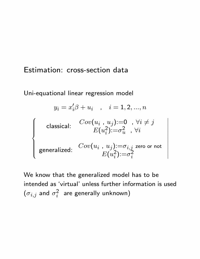
Estimation: cross-section data

Uni-equational linear regression model

yi = x0i� + ui , i = 1; 2; :::; n8>>>>>><>>>>>>:classical:

Cov(ui , uj):=0 , 8i 6= j

E(u2i ):=�2u , 8i

generalized:Cov(ui , uj):=�i;j zero or not

E(u2i ):=�2i

������������We know that the generalized model has to be

intended as `virtual' unless further information is used

(�i;j and �2i are generally unknown)

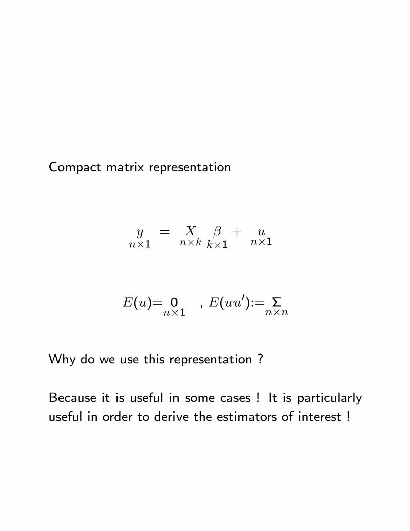
Compact matrix representation

yn�1

= Xn�k

�k�1

+ un�1

E(u)= 0n�1

, E(uu0):= �n�n

Why do we use this representation ?

Because it is useful in some cases ! It is particularly

useful in order to derive the estimators of interest !

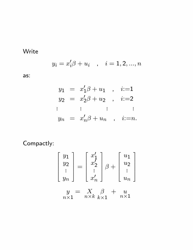
Write

yi = x0i� + ui , i = 1; 2; :::; n

as:

y1 = x01� + u1 , i:=1

y2 = x02� + u2 , i:=2... ... ... ...

yn = x0n� + un , i:=n:

Compactly: 26664y1y2...yn

37775 =26664x01x02...x0n

37775� +26664u1u2...un

37775yn�1

= Xn�k

�k�1

+ un�1

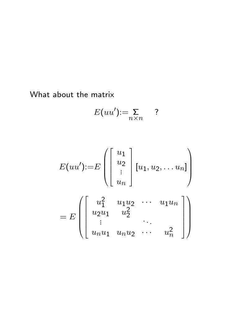
What about the matrix

E(uu0):= �n�n

?

E(uu0):=E

0BBB@26664u1u2...un

37775 [u1; u2; : : : un]1CCCA

= E

0BBBB@266664

u21 u1u2 � � � u1unu2u1 u22... . . .

unu1 unu2 � � � u2n

3777751CCCCA

=

266664E(u21) E(u1u2) � � � E(u1un)E(u2u1) E(u22)... . . .

E(unu1) E(unu2) � � � E(u2n)

377775

=

266664E(u21) Cov(u1; u2) � � � Cov(u1; un)

Cov(u2; u1) E(u22)... . . .

Cov(un; u1) Cov(un; u2) � � � E(u2n)

377775

=

266664�21 �1;2 � � � �1;n�2;1 �22... . . .

�n;1 �n;2 � � � �2n

377775

It is clear that

�:=

(�2uIn6= �2uIn

classical model

generalzied model:

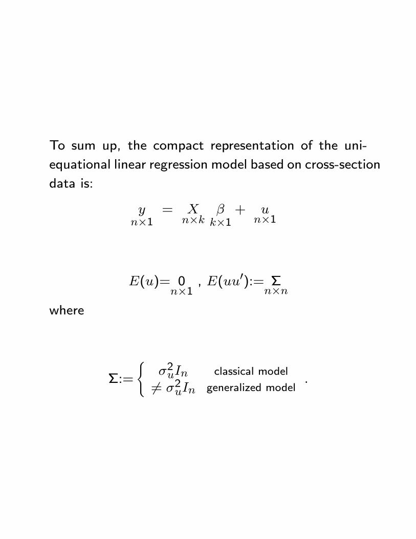
To sum up, the compact representation of the uni-

equational linear regression model based on cross-section

data is:

yn�1

= Xn�k

�k�1

+ un�1

E(u)= 0n�1

, E(uu0):= �n�n

where

�:=

(�2uIn6= �2uIn

classical model

generalized model:

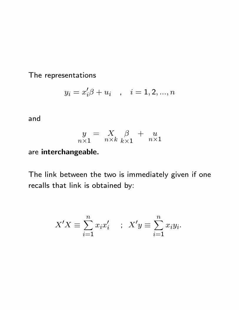
The representations

yi = x0i� + ui , i = 1; 2; :::; n

and

yn�1

= Xn�k

�k�1

+ un�1

are interchangeable.

The link between the two is immediately given if one

recalls that link is obtained by:

X 0X �nXi=1

xix0i ; X 0y �

nXi=1

xiyi:

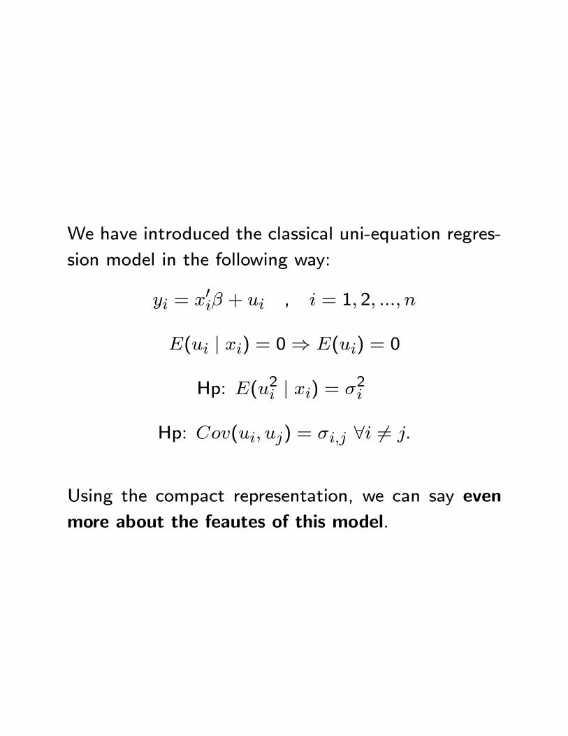
We have introduced the classical uni-equation regres-

sion model in the following way:

yi = x0i� + ui , i = 1; 2; :::; n

E(ui j xi) = 0) E(ui) = 0

Hp: E(u2i j xi) = �2i

Hp: Cov(ui; uj) = �i;j 8i 6= j:

Using the compact representation, we can say even

more about the feautes of this model.

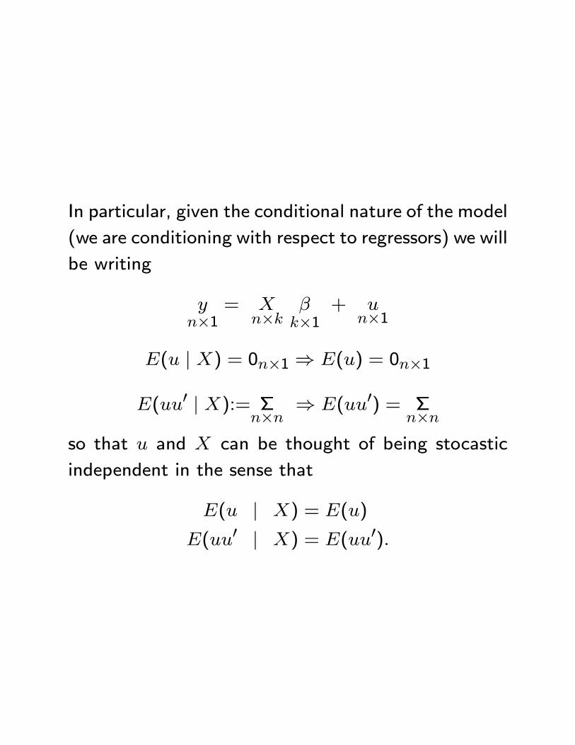
In particular, given the conditional nature of the model

(we are conditioning with respect to regressors) we will

be writing

yn�1

= Xn�k

�k�1

+ un�1

E(u j X) = 0n�1 ) E(u) = 0n�1

E(uu0 j X):= �n�n

) E(uu0) = �n�n

so that u and X can be thought of being stocastic

independent in the sense that

E(u j X) = E(u)

E(uu0 j X) = E(uu0):

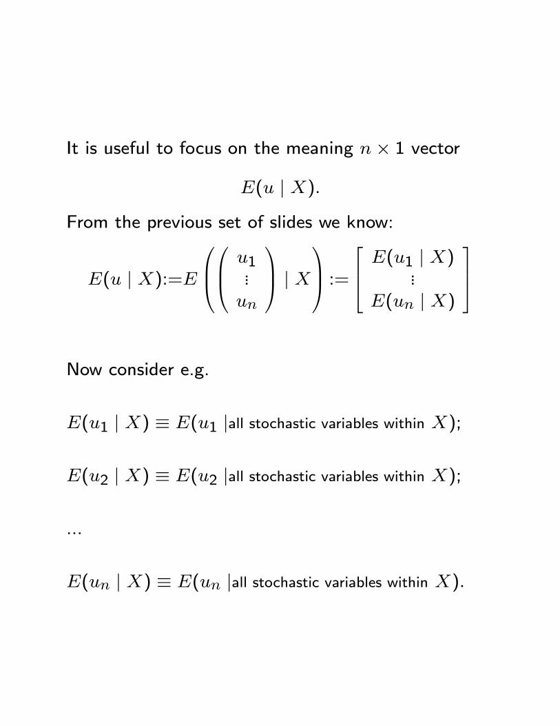
It is useful to focus on the meaning n� 1 vector

E(u j X):

From the previous set of slides we know:

E(u j X):=E

0B@0B@ u1

...un

1CA j X1CA :=

264 E(u1 j X)...E(un j X)

375

Now consider e.g.

E(u1 j X) � E(u1 jall stochastic variables within X);

E(u2 j X) � E(u2 jall stochastic variables within X);

...

E(un j X) � E(un jall stochastic variables within X):

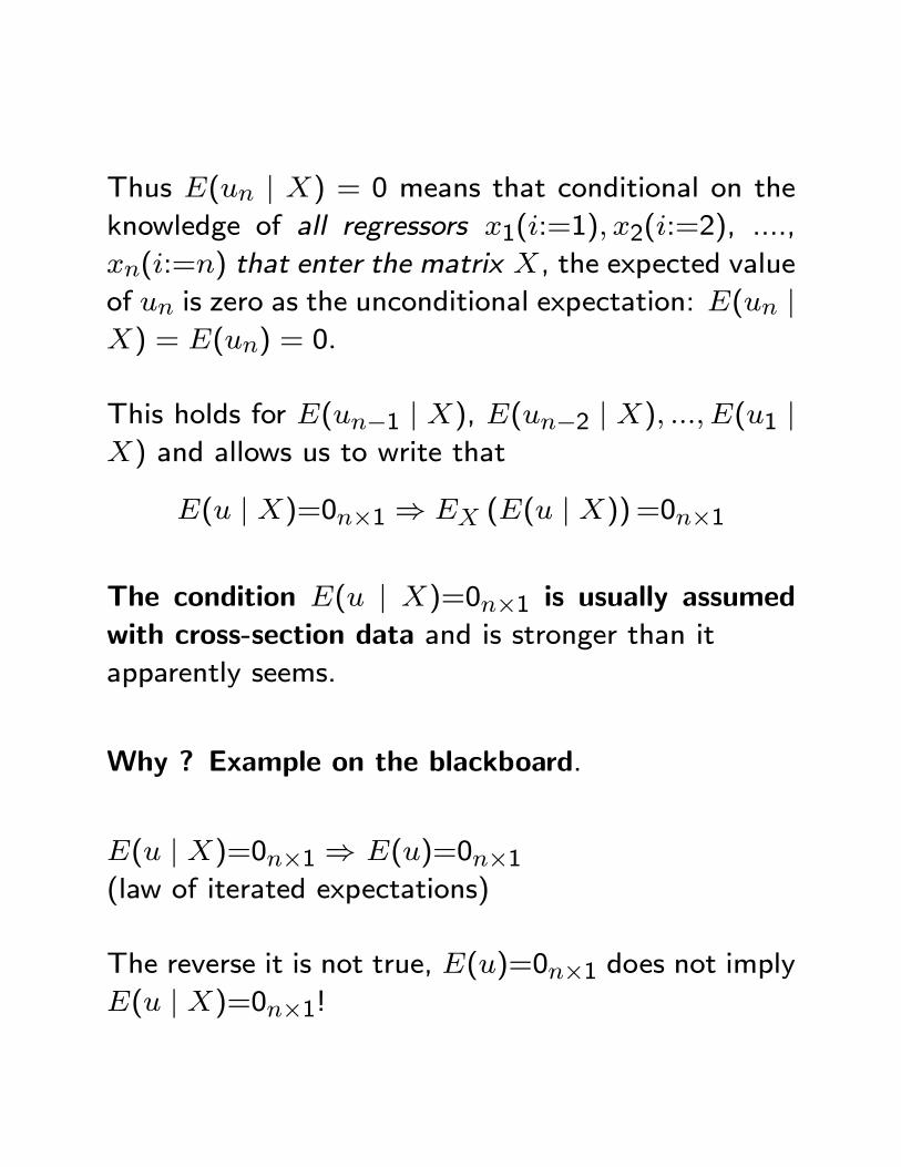
Thus E(un j X) = 0 means that conditional on the

knowledge of all regressors x1(i:=1); x2(i:=2), ....,

xn(i:=n) that enter the matrix X, the expected value

of un is zero as the unconditional expectation: E(un jX) = E(un) = 0:

This holds for E(un�1 j X), E(un�2 j X); :::; E(u1 jX) and allows us to write that

E(u j X)=0n�1 ) EX (E(u j X))=0n�1

The condition E(u j X)=0n�1 is usually assumedwith cross-section data and is stronger than it

apparently seems.

Why ? Example on the blackboard.

E(u j X)=0n�1 ) E(u)=0n�1(law of iterated expectations)

The reverse it is not true, E(u)=0n�1 does not implyE(u j X)=0n�1!

For regression models based on time series data

where lags of y appear among the regressors, the

condition E(u j X)=0n�1 doesn't hold (but it holdsE(u)=0n�1)

Example on the blackboard based on:

ci = �0 + �1ci�1 + �2zi + ui , i = 1; :::; n:

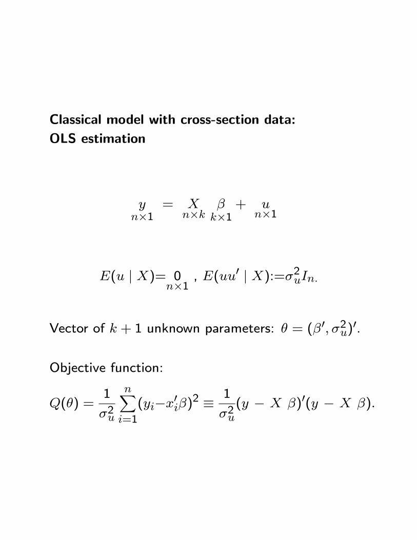
Classical model with cross-section data:

OLS estimation

yn�1

= Xn�k

�k�1

+ un�1

E(u j X)= 0n�1

, E(uu0 j X):=�2uIn:

Vector of k + 1 unknown parameters: � = (�0; �2u)0.

Objective function:

Q(�) =1

�2u

nXi=1

(yi�x0i�)2 �1

�2u(y � X �)0(y � X �):

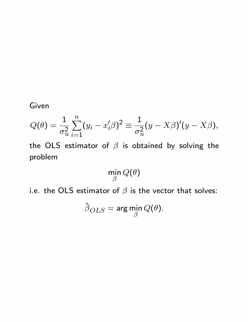
Given

Q(�) =1

�2u

nXi=1

(yi � x0i�)2 � 1

�2u(y �X�)0(y �X�);

the OLS estimator of � is obtained by solving the

problem

min�Q(�)

i.e. the OLS estimator of � is the vector that solves:

�OLS = argmin�Q(�):

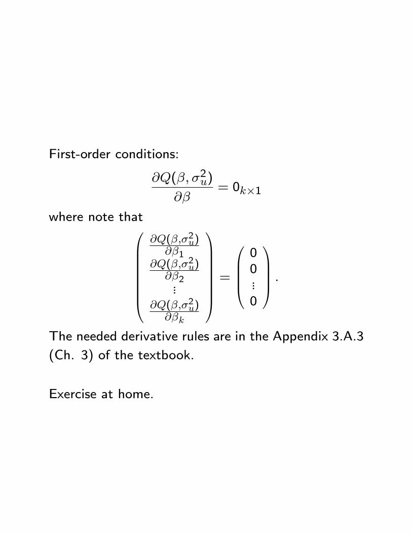
First-order conditions:

@Q(�; �2u)

@�= 0k�1

where note that0BBBBBBB@

@Q(�;�2u)@�1

@Q(�;�2u)@�2...

@Q(�;�2u)@�k

1CCCCCCCA =0BBB@00...0

1CCCA :

The needed derivative rules are in the Appendix 3.A.3

(Ch. 3) of the textbook.

Exercise at home.

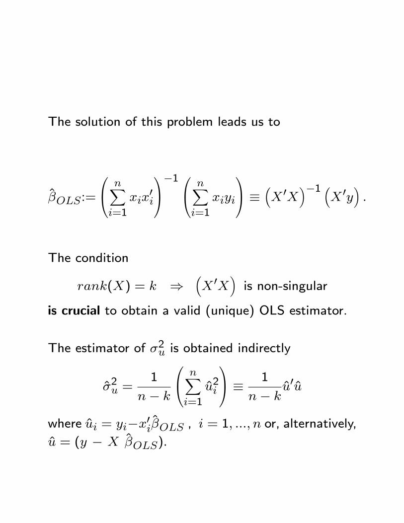
The solution of this problem leads us to

�OLS:=

0@ nXi=1

xix0i

1A�10@ nXi=1

xiyi

1A � �X 0X

��1 �X 0y

�:

The condition

rank(X) = k )�X 0X

�is non-singular

is crucial to obtain a valid (unique) OLS estimator.

The estimator of �2u is obtained indirectly

�2u =1

n� k

0@ nXi=1

u2i

1A � 1

n� ku0u

where ui = yi�x0i�OLS , i = 1; :::; n or, alternatively,u = (y � X �OLS):

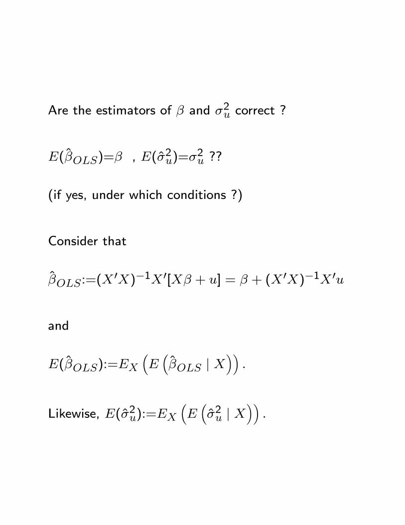
Are the estimators of � and �2u correct ?

E(�OLS)=� , E(�2u)=�2u ??

(if yes, under which conditions ?)

Consider that

�OLS:=(X0X)�1X 0[X� + u] = � + (X 0X)�1X 0u

and

E(�OLS):=EX�E��OLS j X

��:

Likewise, E(�2u):=EX�E��2u j X

��:

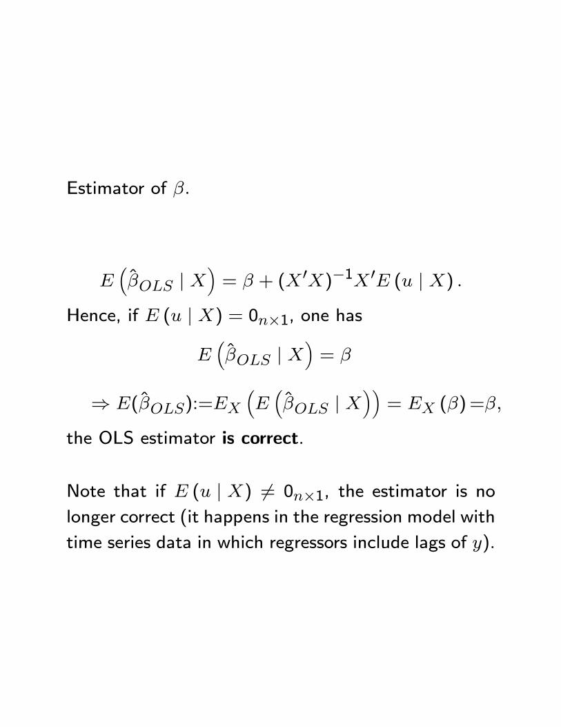
Estimator of �:

E��OLS j X

�= � + (X 0X)�1X 0E (u j X) :

Hence, if E (u j X) = 0n�1, one has

E��OLS j X

�= �

) E(�OLS):=EX�E��OLS j X

��= EX (�)=�;

the OLS estimator is correct.

Note that if E (u j X) 6= 0n�1, the estimator is nolonger correct (it happens in the regression model with

time series data in which regressors include lags of y).

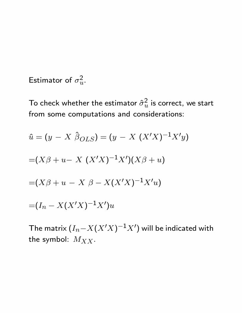
Estimator of �2u:

To check whether the estimator �2u is correct, we start

from some computations and considerations:

u = (y � X �OLS) = (y � X (X 0X)�1X 0y)

=(X� + u� X (X 0X)�1X 0)(X� + u)

=(X� + u � X � �X(X 0X)�1X 0u)

=(In �X(X 0X)�1X 0)u

The matrix (In�X(X 0X)�1X 0) will be indicated withthe symbol: MXX :

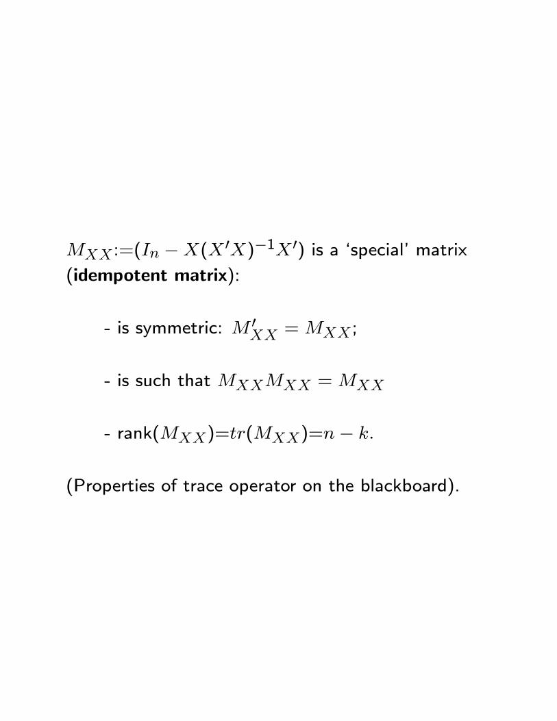
MXX :=(In �X(X 0X)�1X 0) is a `special' matrix(idempotent matrix):

- is symmetric: M 0XX =MXX ;

- is such that MXXMXX =MXX

- rank(MXX)=tr(MXX)=n� k:

(Properties of trace operator on the blackboard).

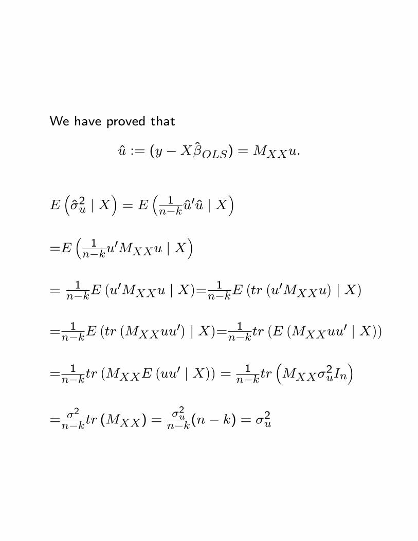
We have proved that

u := (y �X�OLS) =MXXu:

E��2u j X

�= E

�1

n�ku0u j X

�

=E�1

n�ku0MXXu j X

�

= 1n�kE

�u0MXXu j X

�= 1n�kE

�tr�u0MXXu

�j X

�= 1n�kE

�tr�MXXuu

0� j X�= 1n�ktr

�E�MXXuu

0 j X��

= 1n�ktr

�MXXE

�uu0 j X

��= 1

n�ktr�MXX�

2uIn

�

= �2

n�ktr (MXX) =�2un�k(n� k) = �2u

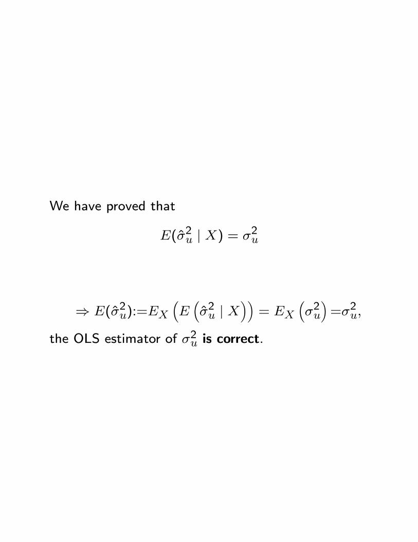
We have proved that

E(�2u j X) = �2u

) E(�2u):=EX�E��2u j X

��= EX

��2u�=�2u;

the OLS estimator of �2u is correct.

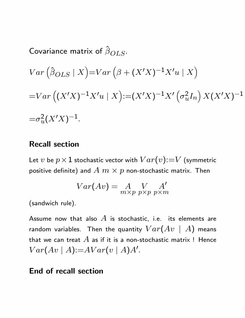
Covariance matrix of �OLS.

V ar��OLS j X

�=V ar

�� + (X 0X)�1X 0u j X

�=V ar

�(X 0X)�1X 0u j X

�:=(X 0X)�1X 0

��2uIn

�X(X 0X)�1

=�2u(X0X)�1:

Recall section

Let v be p�1 stochastic vector with V ar(v):=V (symmetric

positive de�nite) and A m� p non-stochastic matrix. Then

V ar(Av) = Am�p

Vp�p

A0p�m

(sandwich rule).

Assume now that also A is stochastic, i.e. its elements are

random variables. Then the quantity V ar(Av j A) meansthat we can treat A as if it is a non-stochastic matrix ! Hence

V ar(Av j A):=AV ar(v j A)A0:

End of recall section

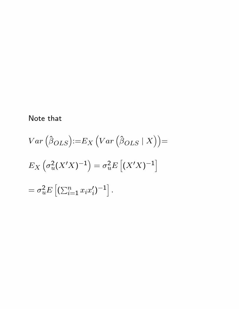
Note that

V ar��OLS

�:=EX

�V ar

��OLS j X

��=

EX��2u(X

0X)�1�= �2uE

h(X 0X)�1

i

= �2uEh(Pni=1 xix

0i)�1i:

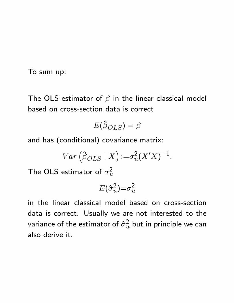
To sum up:

The OLS estimator of � in the linear classical model

based on cross-section data is correct

E(�OLS) = �

and has (conditional) covariance matrix:

V ar��OLS j X

�:=�2u(X

0X)�1:

The OLS estimator of �2u

E(�2u)=�2u

in the linear classical model based on cross-section

data is correct. Usually we are not interested to the

variance of the estimator of �2u but in principle we can

also derive it.

A famous theorem (Gauss-Markov Theorem) applies

to the case in which X does not contain stocastic

variables.

It says that given the linear model

yn�1

= Xn�k

�k�1

+ un�1

E(u)=0n�1 , E(uu0):=�2uIn

the OLS estimator is, in the class of linear correct

estimators, the one whose covariance matrix

V ar��OLS

�:=�2u(X

0X)�1

is the `most e�cient' (minimum covariance matrix).

In our case, X is stochastic (we condition the model

with respect to the regressors).

A version of the Gauss-Markov theorem where X is

stochastic and all variables are conditioned with re-

spect to the elements of X still applies.

This means that any estimator di�erent from the OLS

estimator has (conditional) covariance matrix `larger'

than

V ar��OLS j X

�:=�2u(X

0X)�1:

This is why the OLS estimator applied to cross-section

data (under homoskedasticity) is often called BLUE

(Best Linear Unbiased Estimator).

Recall section

Let1 and2 two symmetric positive de�nite matrices. We say

that1 `is larger' than2 if the matrix1�2 is semipositivede�nite (this means that the eigenvalues of 1� 2 are eitherpositive or zero).

What are eigenvalues ? Given a q � q matrix A the eigenval-

ues are the solutions � (that can be complex numbers) to the

problem

det(�Iq �A) = 0:

If the matrix A is symmetric the eigenvalues are real mumbers.

If A is symmetric and positive de�nite the eigenvalues are real

and positive.

End of recall section

Why do we care about the covariance matrix of the

estimator �OLS ?

Because it is fundamental to make inference !

Imagine that

�OLS j X � N(� , �2u(X0X)�1):

G j X � �2(n� k) , G:=�2u�2u(n� k):

These distributions hold if u j X � N(0 , �2uIn)

(irrespective of whether n is small or large).

It is possible to show that the random vector

�OLS j X is independent on the random

variable G j X:

Observe that given

�OLS j X � N(� , �2u(X0X)�1);

then

�j � �j

�u�cjj�1=2 j X � N(0 , 1) , j = 1; :::; k

where �j is the j-th element of �, �j is the j-th

element of � and cjj is the j-th element on the main

diagonal of the matrix (X 0X)�1:

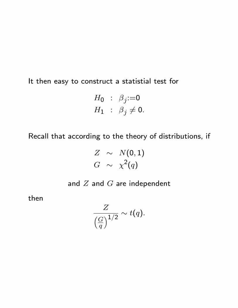
It then easy to construct a statistial test for

H0 : �j:=0

H1 : �j 6= 0.

Recall that according to the theory of distributions, if

Z � N(0; 1)

G � �2(q)

and Z and G are independent

thenZ�

Gq

�1=2 � t(q):

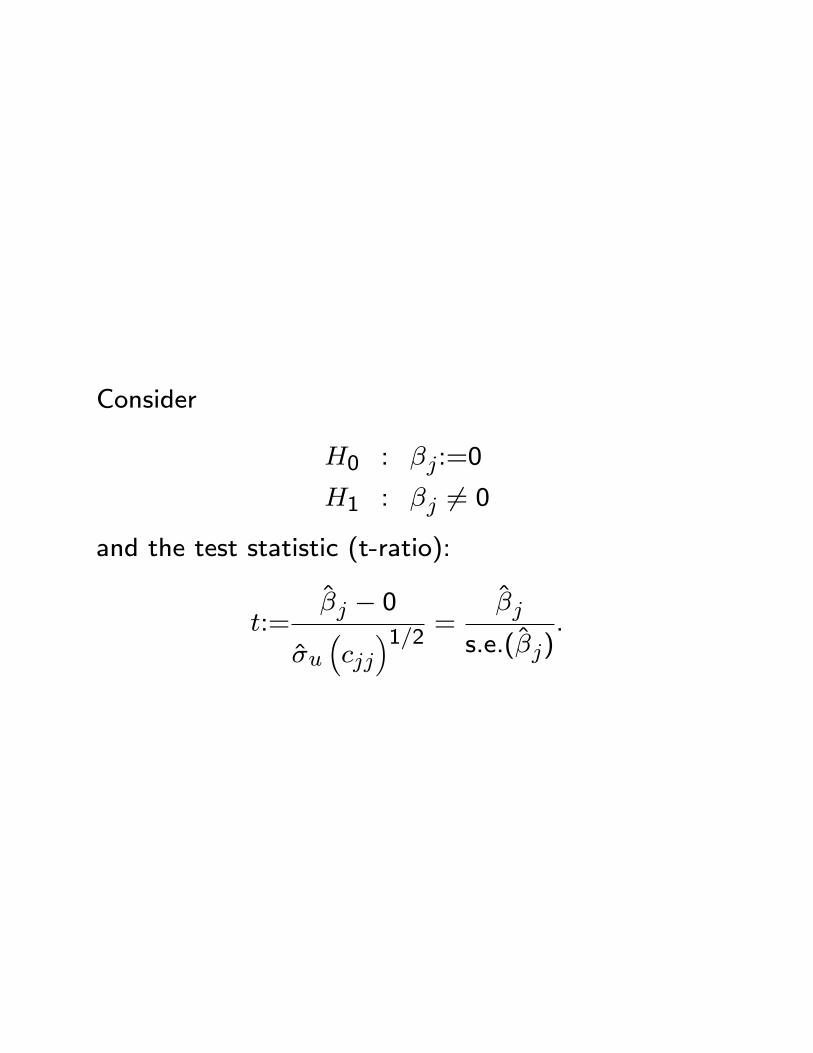
Consider

H0 : �j:=0

H1 : �j 6= 0

and the test statistic (t-ratio):

t:=�j � 0

�u�cjj�1=2 = �j

s.e.(�j).

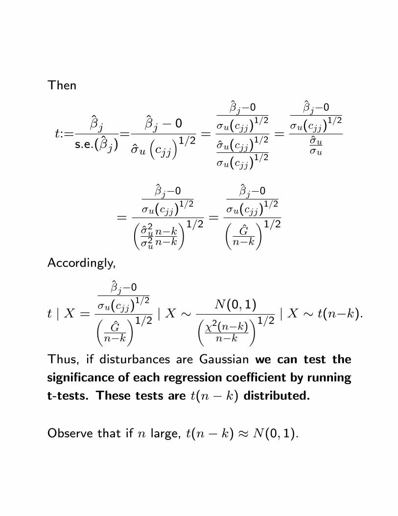
Then

t:=�j

s.e.(�j)=

�j � 0

�u�cjj�1=2 =

�j�0�u(cjj)

1=2

�u(cjj)1=2

�u(cjj)1=2

=

�j�0�u(cjj)

1=2

�u�u

=

�j�0�u(cjj)

1=2��2u�2u

n�kn�k

�1=2 =�j�0

�u(cjj)1=2�

Gn�k

�1=2Accordingly,

t j X =

�j�0�u(cjj)

1=2�Gn�k

�1=2 j X � N(0; 1)��2(n�k)n�k

�1=2 j X � t(n�k):

Thus, if disturbances are Gaussian we can test the

signi�cance of each regression coe�cient by running

t-tests. These tests are t(n� k) distributed.

Observe that if n large, t(n� k) � N(0; 1).

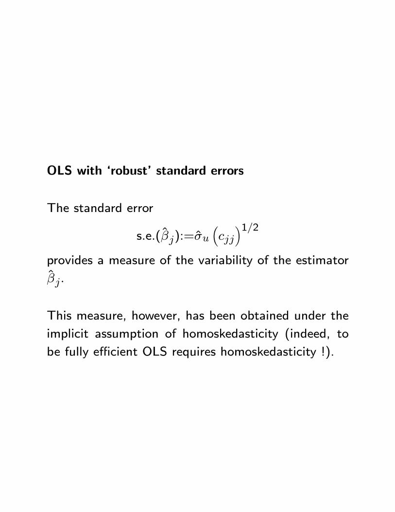
OLS with `robust' standard errors

The standard error

s.e.(�j):=�u�cjj�1=2

provides a measure of the variability of the estimator

�j:

This measure, however, has been obtained under the

implicit assumption of homoskedasticity (indeed, to

be fully e�cient OLS requires homoskedasticity !).

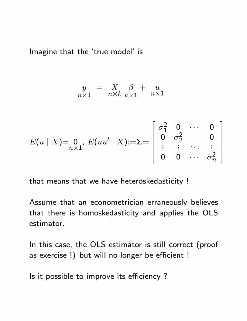
Imagine that the `true model' is

yn�1

= Xn�k

�k�1

+ un�1

E(u j X)= 0n�1

, E(uu0 j X):=�=

266664�21 0 � � � 00 �22 0... ... . . . ...0 0 � � � �2n

377775

that means that we have heteroskedasticity !

Assume that an econometrician erraneously believes

that there is homoskedasticity and applies the OLS

estimator.

In this case, the OLS estimator is still correct (proof

as exercise !) but will no longer be e�cient !

Is it possible to improve its e�ciency ?

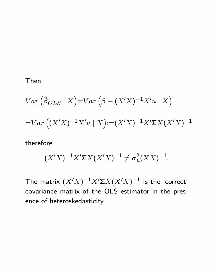
Then

V ar��OLS j X

�=V ar

�� + (X 0X)�1X 0u j X

�

=V ar�(X 0X)�1X 0u j X

�:=(X 0X)�1X 0�X(X 0X)�1

therefore

(X 0X)�1X 0�X(X 0X)�1 6= �2u(XX)�1:

The matrix (X 0X)�1X 0�X(X 0X)�1 is the `correct'covariance matrix of the OLS estimator in the pres-

ence of heteroskedasticity.

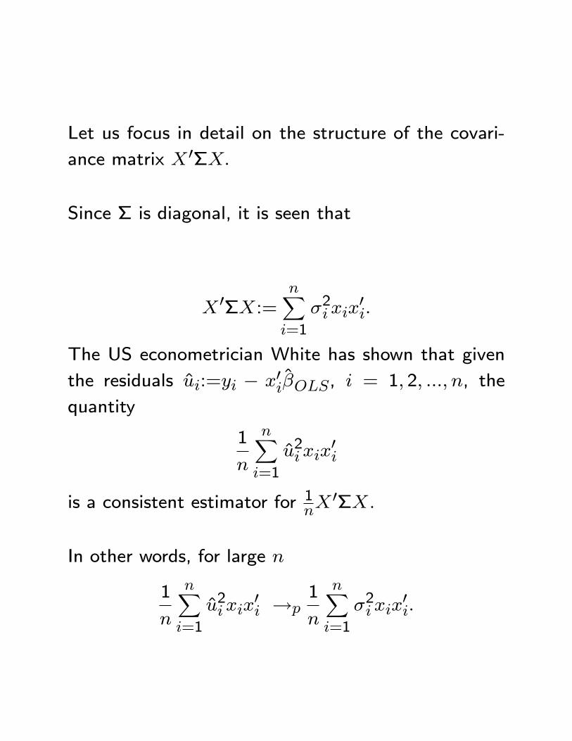
Let us focus in detail on the structure of the covari-

ance matrix X 0�X:

Since � is diagonal, it is seen that

X 0�X:=nXi=1

�2ixix0i:

The US econometrician White has shown that given

the residuals ui:=yi � x0i�OLS, i = 1; 2; :::; n, the

quantity

1

n

nXi=1

u2ixix0i

is a consistent estimator for 1nX0�X.

In other words, for large n

1

n

nXi=1

u2ixix0i !p

1

n

nXi=1

�2ixix0i:

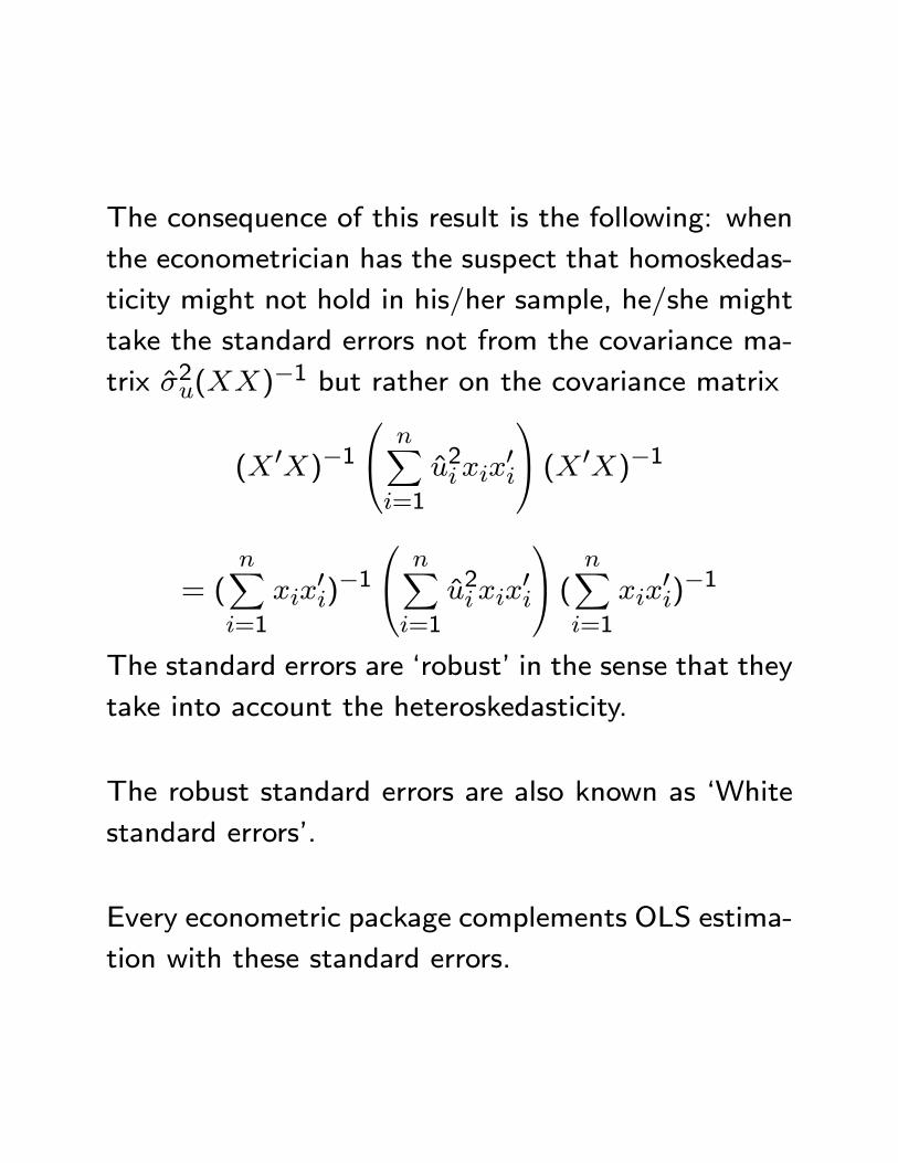
The consequence of this result is the following: when

the econometrician has the suspect that homoskedas-

ticity might not hold in his/her sample, he/she might

take the standard errors not from the covariance ma-

trix �2u(XX)�1 but rather on the covariance matrix

(X 0X)�10@ nXi=1

u2ixix0i

1A (X 0X)�1

= (nXi=1

xix0i)�10@ nXi=1

u2ixix0i

1A ( nXi=1

xix0i)�1

The standard errors are `robust' in the sense that they

take into account the heteroskedasticity.

The robust standard errors are also known as `White

standard errors'.

Every econometric package complements OLS estima-

tion with these standard errors.

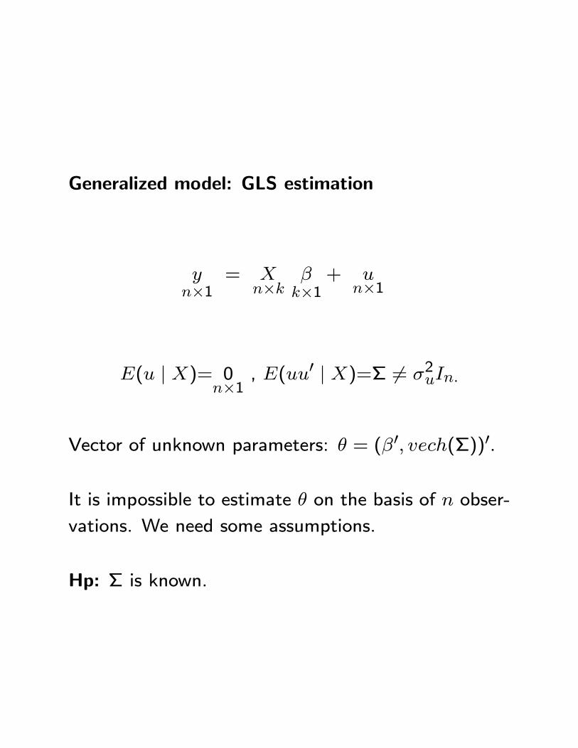
Generalized model: GLS estimation

yn�1

= Xn�k

�k�1

+ un�1

E(u j X)= 0n�1

, E(uu0 j X)=� 6= �2uIn:

Vector of unknown parameters: � = (�0; vech(�))0.

It is impossible to estimate � on the basis of n obser-

vations. We need some assumptions.

Hp: � is known.

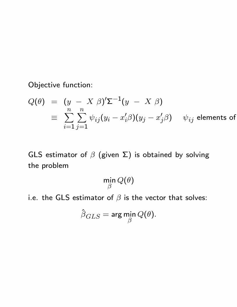
Objective function:

Q(�) = (y � X �)0��1(y � X �)

�nXi=1

nXj=1

ij(yi � x0i�)(yj � x0j�) ij elements of ��1:

GLS estimator of � (given �) is obtained by solving

the problem

min�Q(�)

i.e. the GLS estimator of � is the vector that solves:

�GLS = argmin�Q(�):

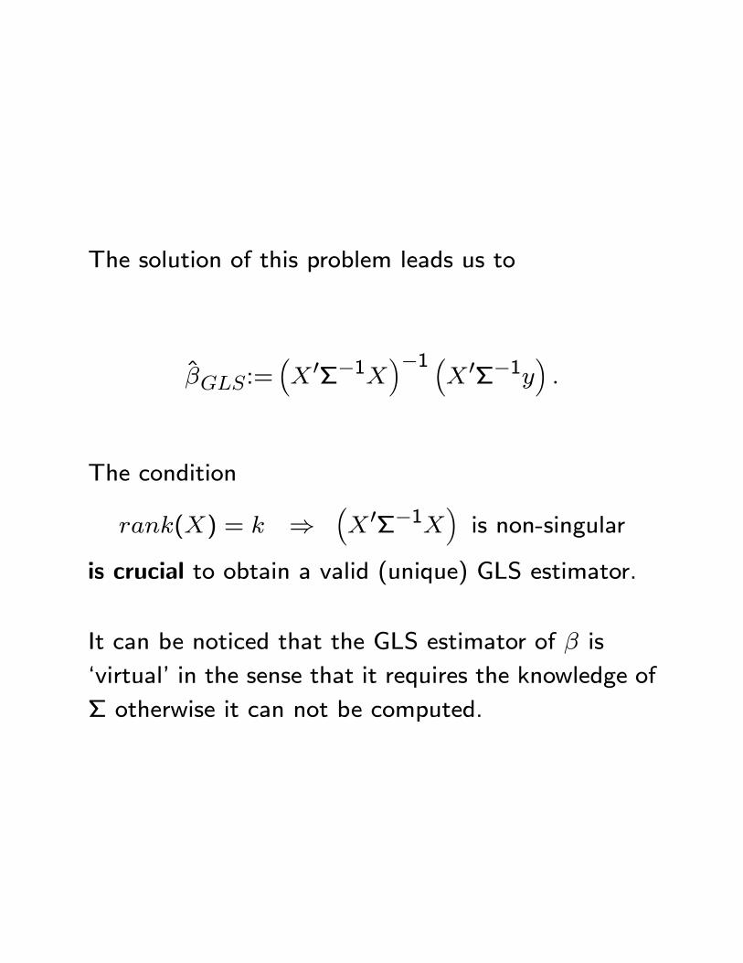
The solution of this problem leads us to

�GLS:=�X 0��1X

��1 �X 0��1y

�:

The condition

rank(X) = k )�X 0��1X

�is non-singular

is crucial to obtain a valid (unique) GLS estimator.

It can be noticed that the GLS estimator of � is

`virtual' in the sense that it requires the knowledge of

� otherwise it can not be computed.

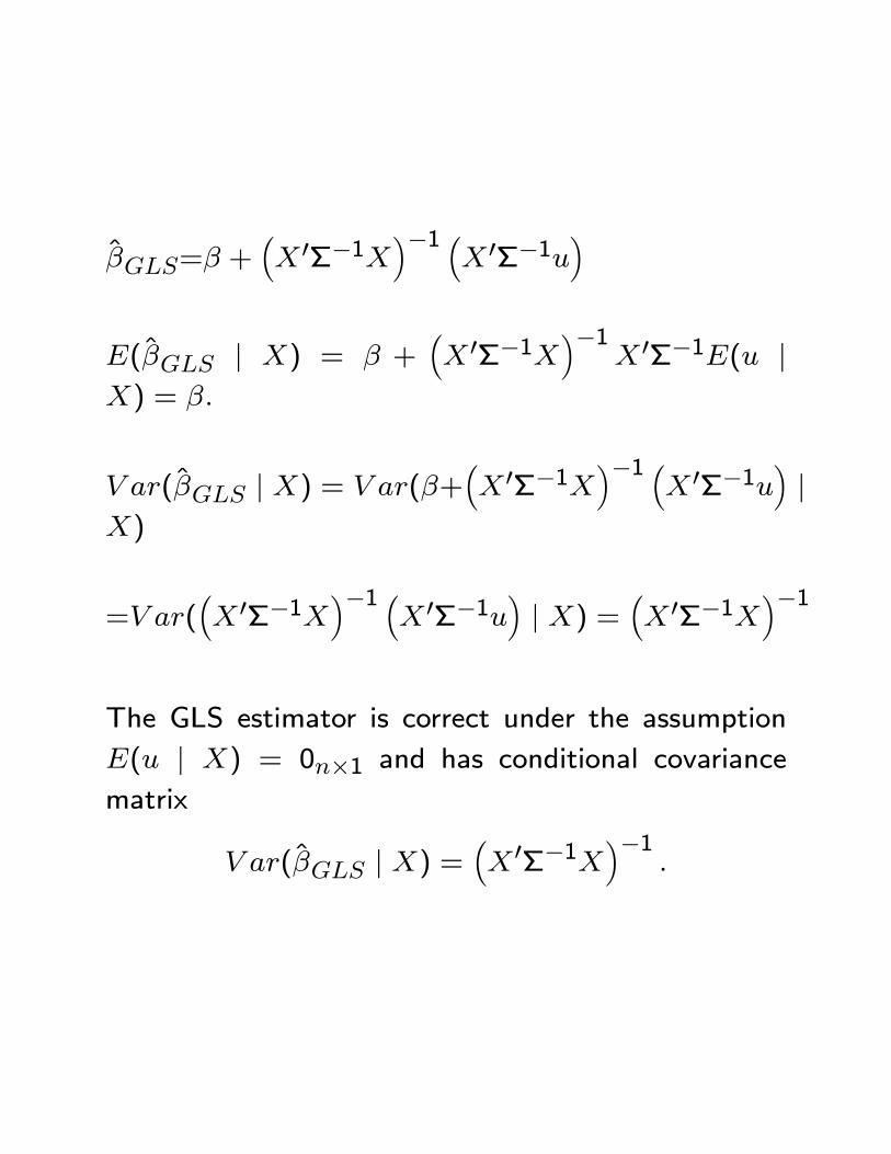
�GLS=� +�X 0��1X

��1 �X 0��1u

�

E(�GLS j X) = � +�X 0��1X

��1X 0��1E(u j

X) = �:

V ar(�GLS j X) = V ar(�+�X 0��1X

��1 �X 0��1u

�j

X)

=V ar(�X 0��1X

��1 �X 0��1u

�j X) =

�X 0��1X

��1

The GLS estimator is correct under the assumption

E(u j X) = 0n�1 and has conditional covariancematrix

V ar(�GLS j X) =�X 0��1X

��1:

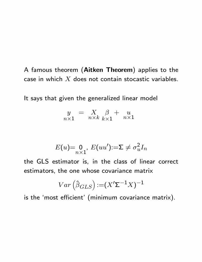
A famous theorem (Aitken Theorem) applies to the

case in which X does not contain stocastic variables.

It says that given the generalized linear model

yn�1

= Xn�k

�k�1

+ un�1

E(u)= 0n�1

, E(uu0):=� 6= �2uIn

the GLS estimator is, in the class of linear correct

estimators, the one whose covariance matrix

V ar��GLS

�:=(X 0��1X)�1

is the `most e�cient' (minimum covariance matrix).

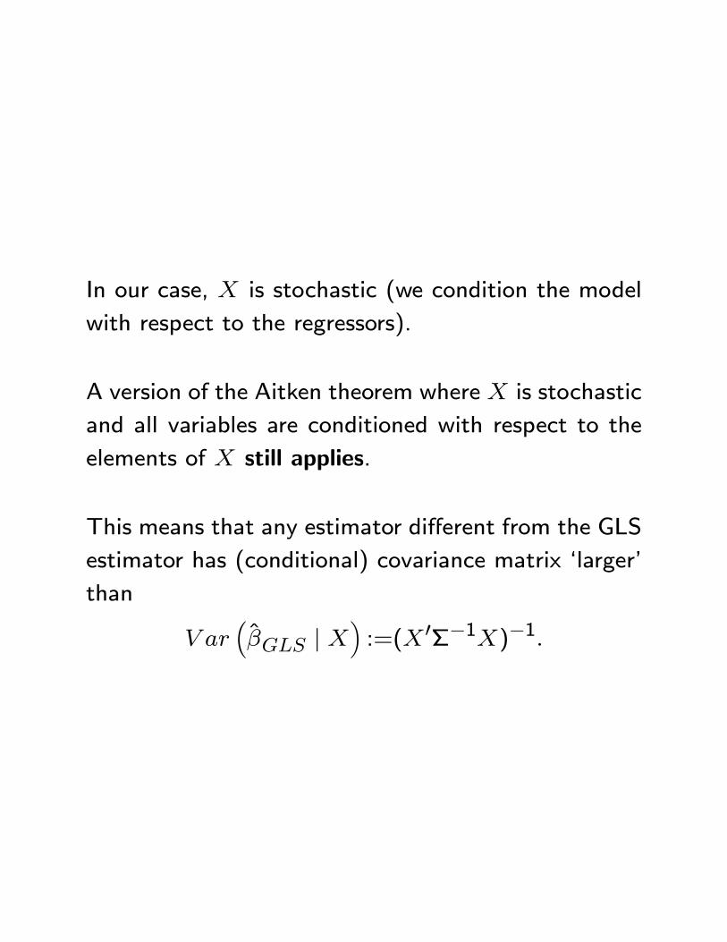
In our case, X is stochastic (we condition the model

with respect to the regressors).

A version of the Aitken theorem where X is stochastic

and all variables are conditioned with respect to the

elements of X still applies.

This means that any estimator di�erent from the GLS

estimator has (conditional) covariance matrix `larger'

than

V ar��GLS j X

�:=(X 0��1X)�1:

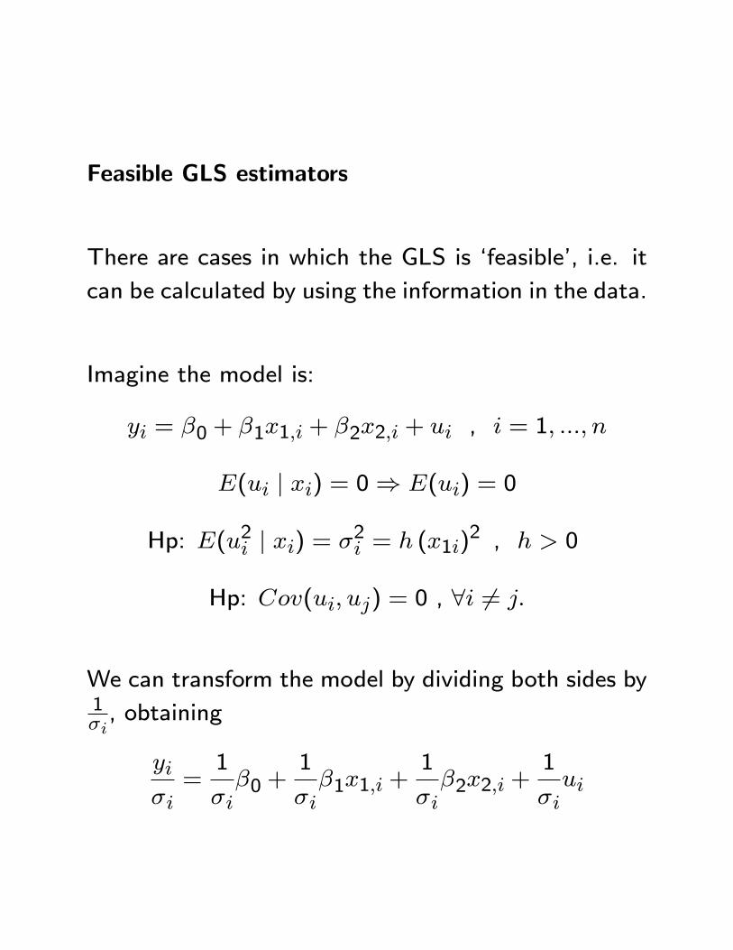
Feasible GLS estimators

There are cases in which the GLS is `feasible', i.e. it

can be calculated by using the information in the data.

Imagine the model is:

yi = �0 + �1x1;i + �2x2;i + ui , i = 1; :::; n

E(ui j xi) = 0) E(ui) = 0

Hp: E(u2i j xi) = �2i = h (x1i)2 , h > 0

Hp: Cov(ui; uj) = 0 , 8i 6= j:

We can transform the model by dividing both sides by1�i, obtaining

yi�i=1

�i�0 +

1

�i�1x1;i +

1

�i�2x2;i +

1

�iui

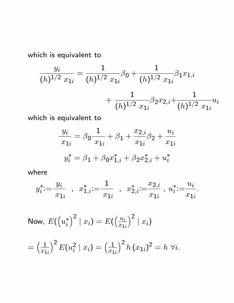
which is equivalent to

yi

(h)1=2 x1i=

1

(h)1=2 x1i�0 +

1

(h)1=2 x1i�1x1;i

+1

(h)1=2 x1i�2x2;i+

1

(h)1=2 x1iui

which is equivalent to

yix1i

= �01

x1i+ �1 +

x2;i

x1i�2 +

uix1i

y�i = �1 + �0x�1;i + �2x

�2;i + u�i

where

y�i :=yix1i

, x�1;i:=1

x1i, x�2;i:=

x2;i

x1i, u�i :=

uix1i.

Now, E(�u�i�2 j xi) = E(

�uix1i

�2 j xi)=�1x1i

�2E(u2i j xi) =

�1x1i

�2h (x1i)

2 = h 8i:

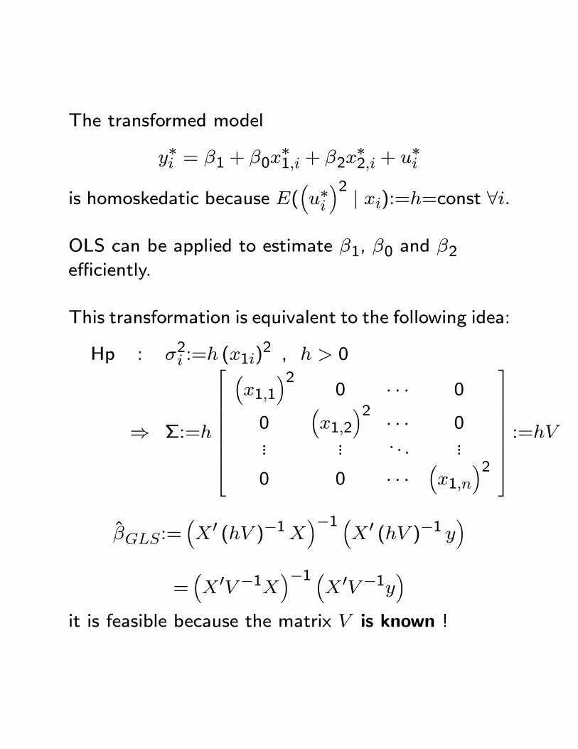
The transformed model

y�i = �1 + �0x�1;i + �2x

�2;i + u�i

is homoskedatic because E(�u�i�2 j xi):=h=const 8i:

OLS can be applied to estimate �1, �0 and �2e�ciently.

This transformation is equivalent to the following idea:

Hp : �2i :=h (x1i)2 , h > 0

) �:=h

266666664

�x1;1

�20 � � � 0

0�x1;2

�2 � � � 0... ... . . . ...

0 0 � � ��x1;n

�2

377777775 :=hV

�GLS:=�X 0 (hV )�1X

��1 �X 0 (hV )�1 y

�=�X 0V �1X

��1 �X 0V �1y

�it is feasible because the matrix V is known !

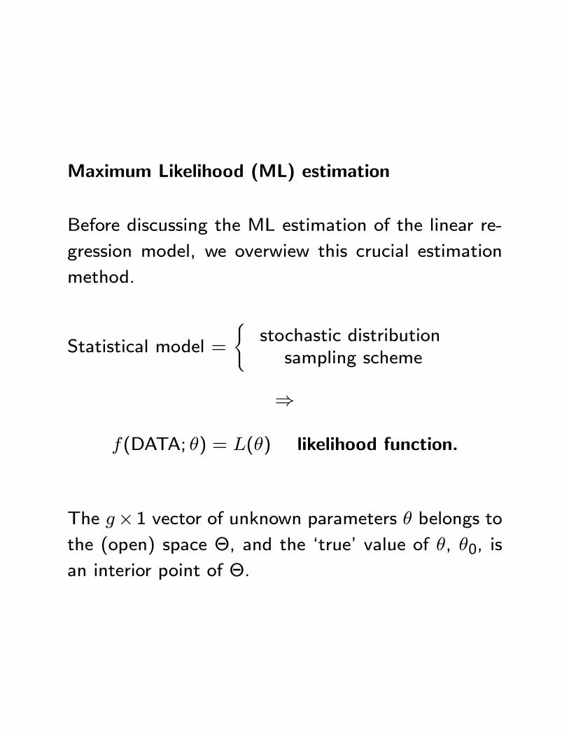
Maximum Likelihood (ML) estimation

Before discussing the ML estimation of the linear re-

gression model, we overwiew this crucial estimation

method.

Statistical model =

(stochastic distributionsampling scheme

)

f(DATA; �) = L(�) likelihood function.

The g�1 vector of unknown parameters � belongs tothe (open) space �, and the `true' value of �, �0, is

an interior point of �.

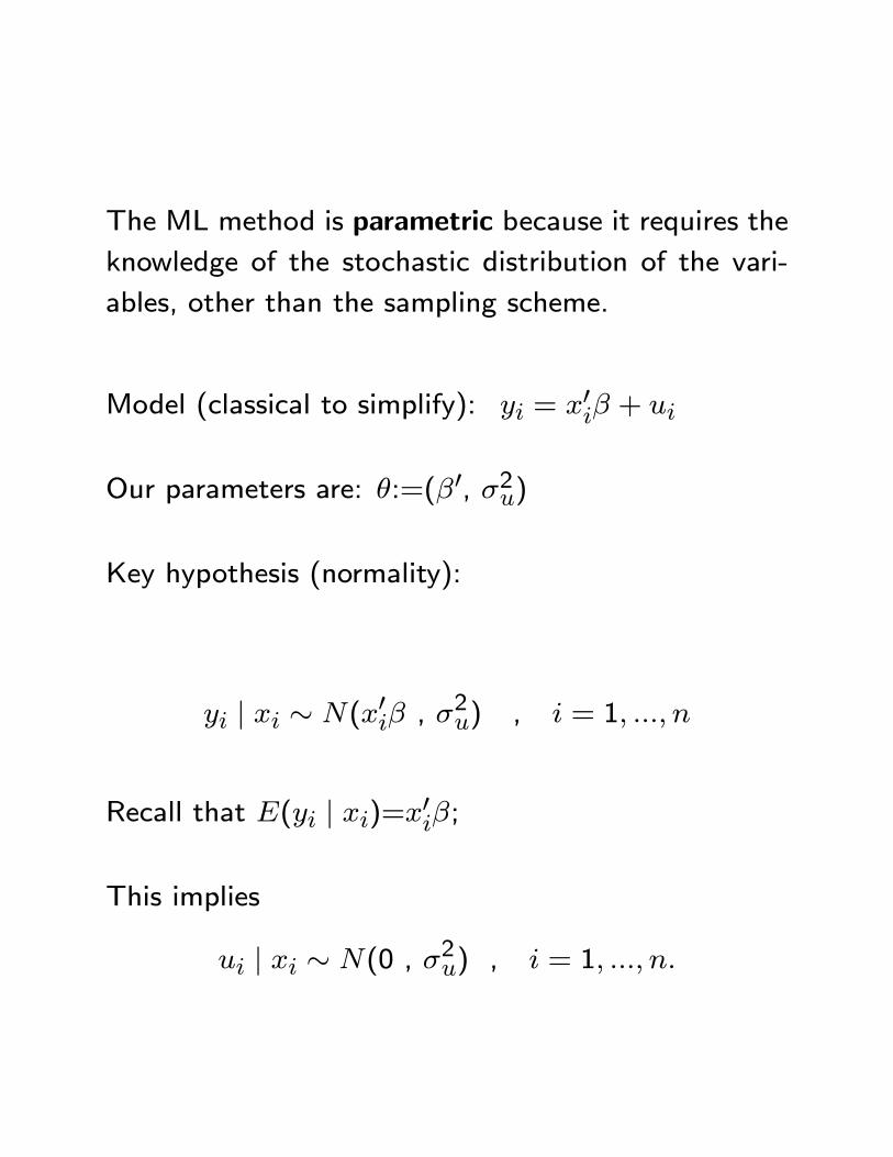
The ML method is parametric because it requires the

knowledge of the stochastic distribution of the vari-

ables, other than the sampling scheme.

Model (classical to simplify): yi = x0i� + ui

Our parameters are: �:=(�0, �2u)

Key hypothesis (normality):

yi j xi � N(x0i� , �2u) , i = 1; :::; n

Recall that E(yi j xi)=x0i�;

This implies

ui j xi � N(0 , �2u) , i = 1; :::; n:

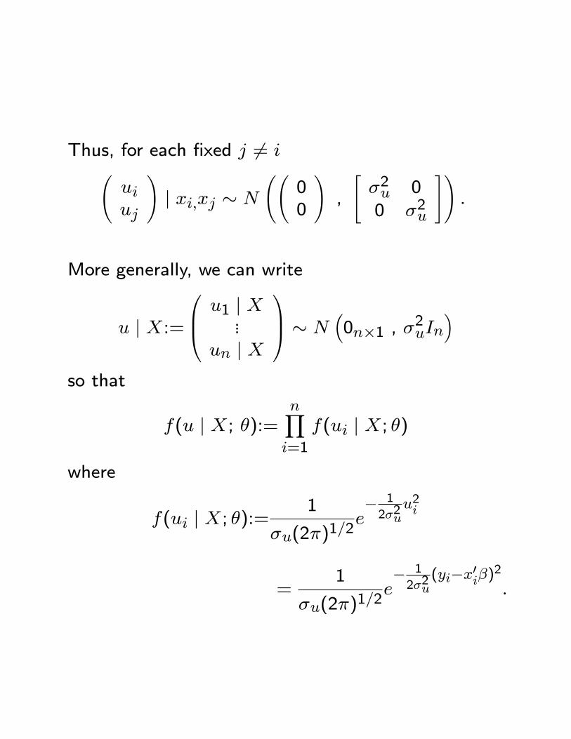
Thus, for each �xed j 6= i uiuj

!j xi;xj � N

00

!,

"�2u 00 �2u

#!:

More generally, we can write

u j X:=

0B@ u1 j X...

un j X

1CA � N�0n�1 , �

2uIn

�so that

f(u j X; �):=nYi=1

f(ui j X; �)

where

f(ui j X; �):=1

�u(2�)1=2e� 1

2�2uu2i

=1

�u(2�)1=2e� 1

2�2u(yi�x0i�)

2

:

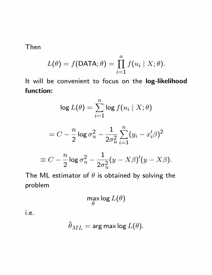
Then

L(�) = f(DATA; �) =nYi=1

f(ui j X; �):

It will be convenient to focus on the log-likelihood

function:

logL(�) =nXi=1

log f(ui j X; �)

= C � n

2log �2u �

1

2�2u

nXi=1

(yi � x0i�)2

� C � n

2log �2u �

1

2�2u(y �X�)0(y �X�):

The ML estimator of � is obtained by solving the

problem

max�logL(�)

i.e.

�ML = argmax logL(�):

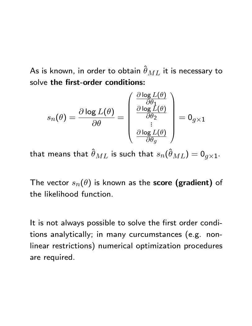
As is known, in order to obtain �ML it is necessary to

solve the �rst-order conditions:

sn(�) =@ logL(�)

@�=

0BBBBBB@

@ logL(�)@�1

@ logL(�)@�2...

@ logL(�)@�g

1CCCCCCA = 0g�1

that means that �ML is such that sn(�ML) = 0g�1:

The vector sn(�) is known as the score (gradient) of

the likelihood function.

It is not always possible to solve the �rst order condi-

tions analytically; in many curcumstances (e.g. non-

linear restrictions) numerical optimization procedures

are required.

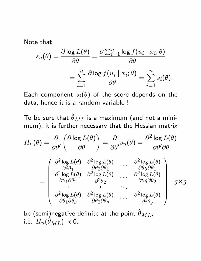
Note that

sn(�) =@ logL(�)

@�=@Pni=1 log f(ui j xi; �)

@�

=nXi=1

@ log f(ui j xi; �)@�

=nXi=1

si(�):

Each component si(�) of the score depends on thedata, hence it is a random variable !

To be sure that �ML is a maximum (and not a mini-mum), it is further necessary that the Hessian matrix

Hn(�) =@

@�0

@ logL(�)

@�

!=

@

@�0sn(�) =

@2 logL(�)

@�0@�

=

0BBBBBBBB@

@2 logL(�)@2�1

@2 logL(�)@�2@�1

� � � @2 logL(�)@�g@�1

@2 logL(�)@�1@�2

@2 logL(�)@2�2

� � � @2 logL(�)@�g@�2

... ... . . .@2 logL(�)@�1@�g

@2 logL(�)@�2@�g

� � � @2 logL(�)@2�g

1CCCCCCCCAg�g

be (semi)negative de�nite at the point �ML,i.e. Hn(�ML) � 0:

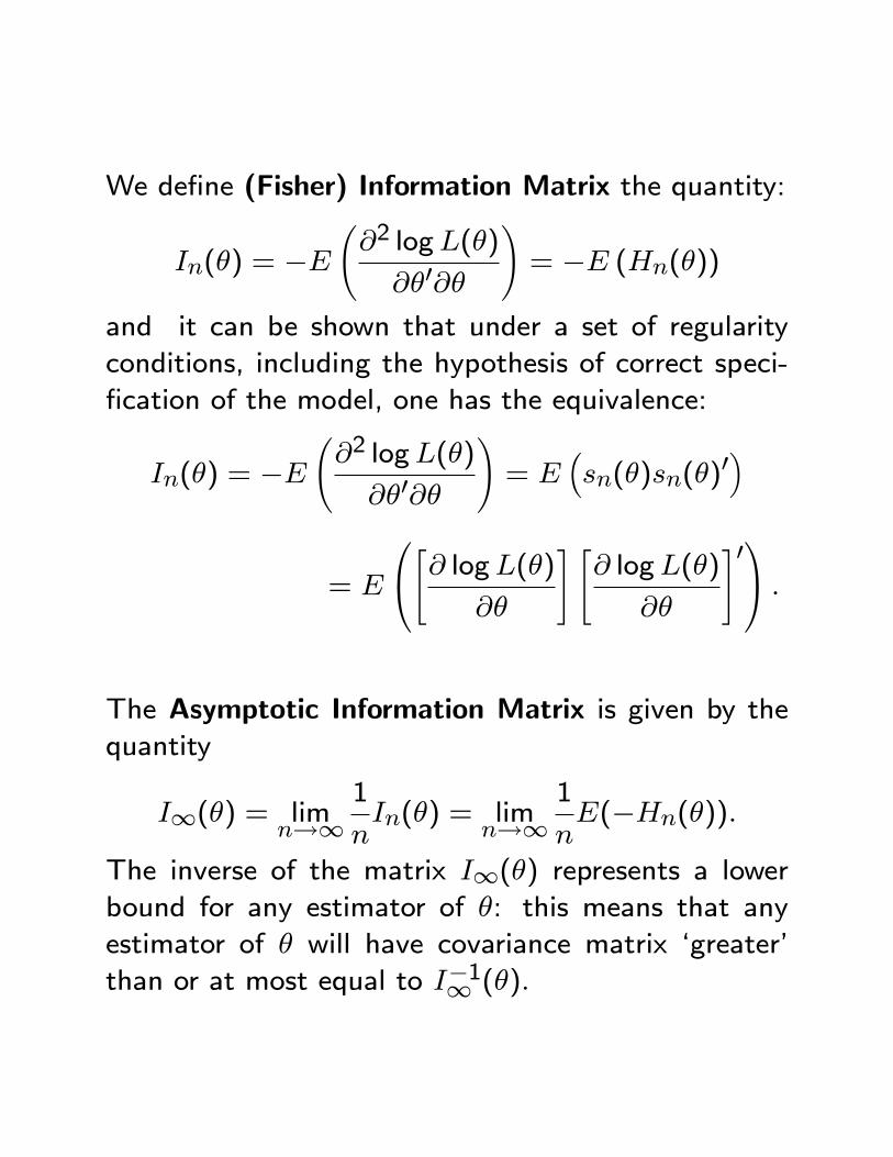
We de�ne (Fisher) Information Matrix the quantity:

In(�) = �E @2 logL(�)

@�0@�

!= �E (Hn(�))

and it can be shown that under a set of regularity

conditions, including the hypothesis of correct speci-

�cation of the model, one has the equivalence:

In(�) = �E @2 logL(�)

@�0@�

!= E

�sn(�)sn(�)

0�

= E

0@"@ logL(�)@�

# "@ logL(�)

@�

#01A :

The Asymptotic Information Matrix is given by thequantity

I1(�) = limn!1

1

nIn(�) = lim

n!11

nE(�Hn(�)):

The inverse of the matrix I1(�) represents a lowerbound for any estimator of �: this means that any

estimator of � will have covariance matrix `greater'

than or at most equal to I�11 (�):

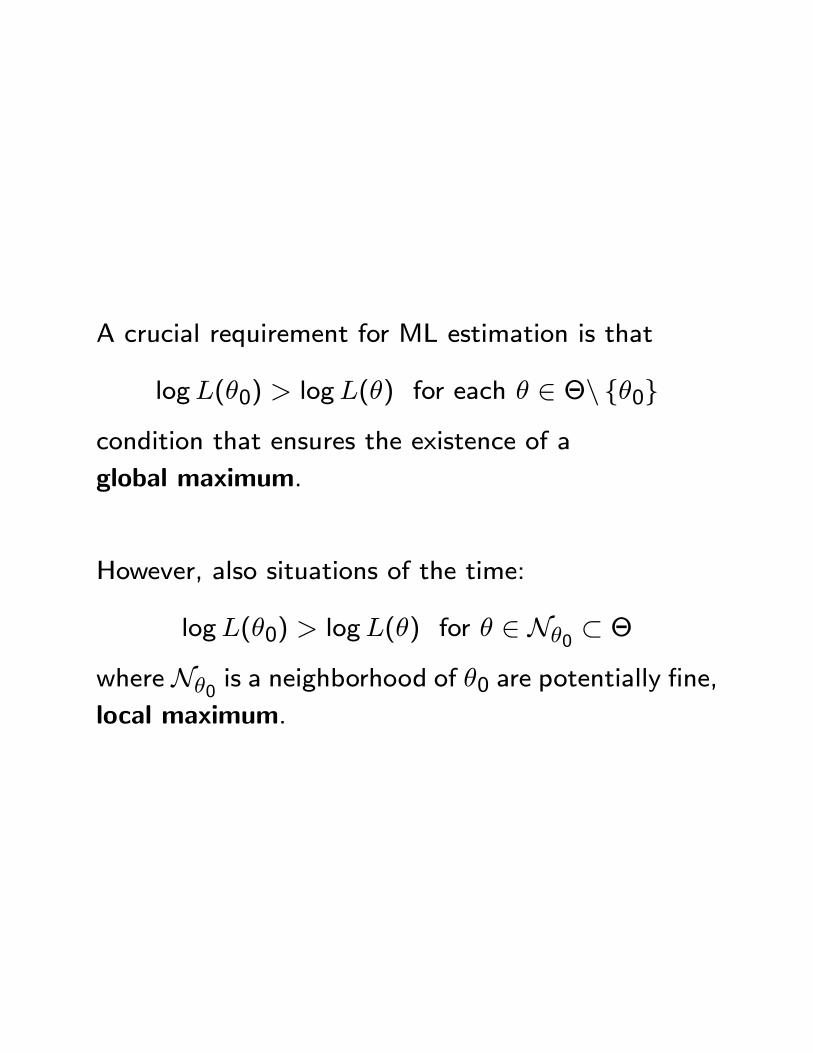
A crucial requirement for ML estimation is that

logL(�0) > logL(�) for each � 2 �n f�0g

condition that ensures the existence of a

global maximum.

However, also situations of the time:

logL(�0) > logL(�) for � 2 N�0 � �

where N�0 is a neighborhood of �0 are potentially �ne,local maximum.

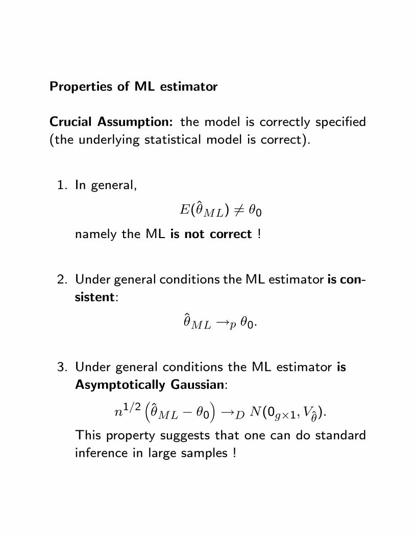
Properties of ML estimator

Crucial Assumption: the model is correctly speci�ed

(the underlying statistical model is correct).

1. In general,

E(�ML) 6= �0

namely the ML is not correct !

2. Under general conditions the ML estimator is con-

sistent:

�ML !p �0:

3. Under general conditions the ML estimator is

Asymptotically Gaussian:

n1=2��ML � �0

�!D N(0g�1; V�):

This property suggests that one can do standard

inference in large samples !

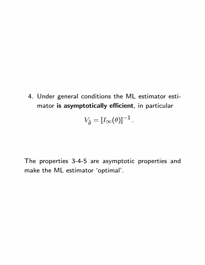
4. Under general conditions the ML estimator esti-

mator is asymptotically e�cient, in particular

V�= [I1(�)]�1 :

The properties 3-4-5 are asymptotic properties and

make the ML estimator `optimal'.

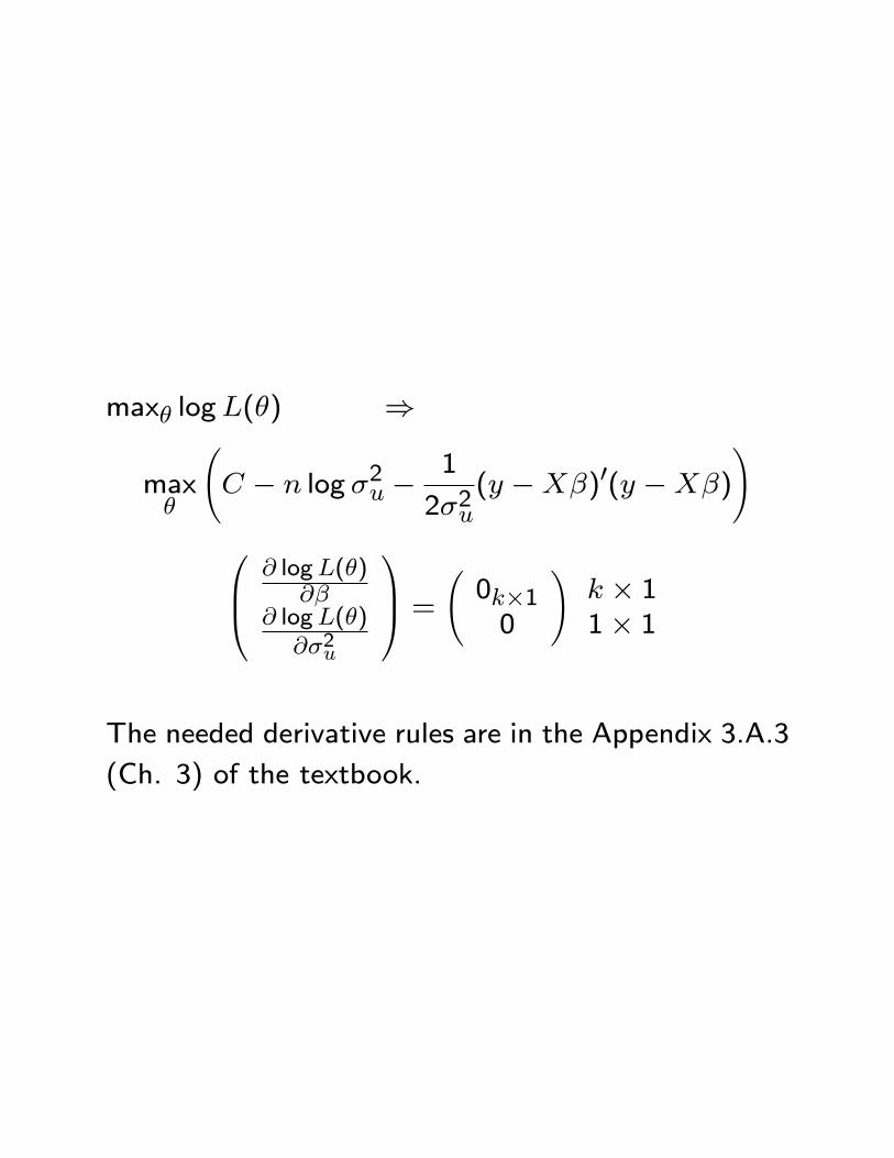
max� logL(�) )

max�

C � n log �2u �

1

2�2u(y �X�)0(y �X�)

!0B@ @ logL(�)

@�@ logL(�)@�2u

1CA = 0k�10

!k � 11� 1

The needed derivative rules are in the Appendix 3.A.3

(Ch. 3) of the textbook.

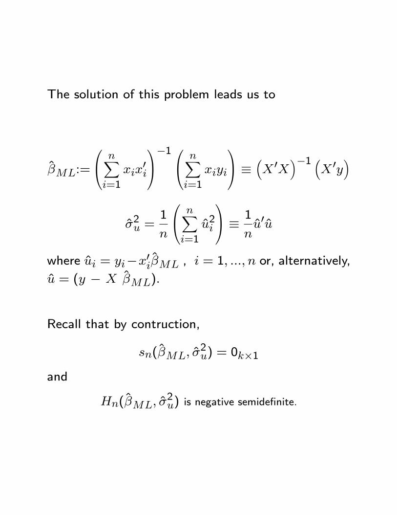
The solution of this problem leads us to

�ML:=

0@ nXi=1

xix0i

1A�10@ nXi=1

xiyi

1A � �X 0X

��1 �X 0y

�

�2u =1

n

0@ nXi=1

u2i

1A � 1

nu0u

where ui = yi�x0i�ML , i = 1; :::; n or, alternatively,

u = (y � X �ML):

Recall that by contruction,

sn(�ML; �2u) = 0k�1

and

Hn(�ML; �2u) is negative semide�nite.

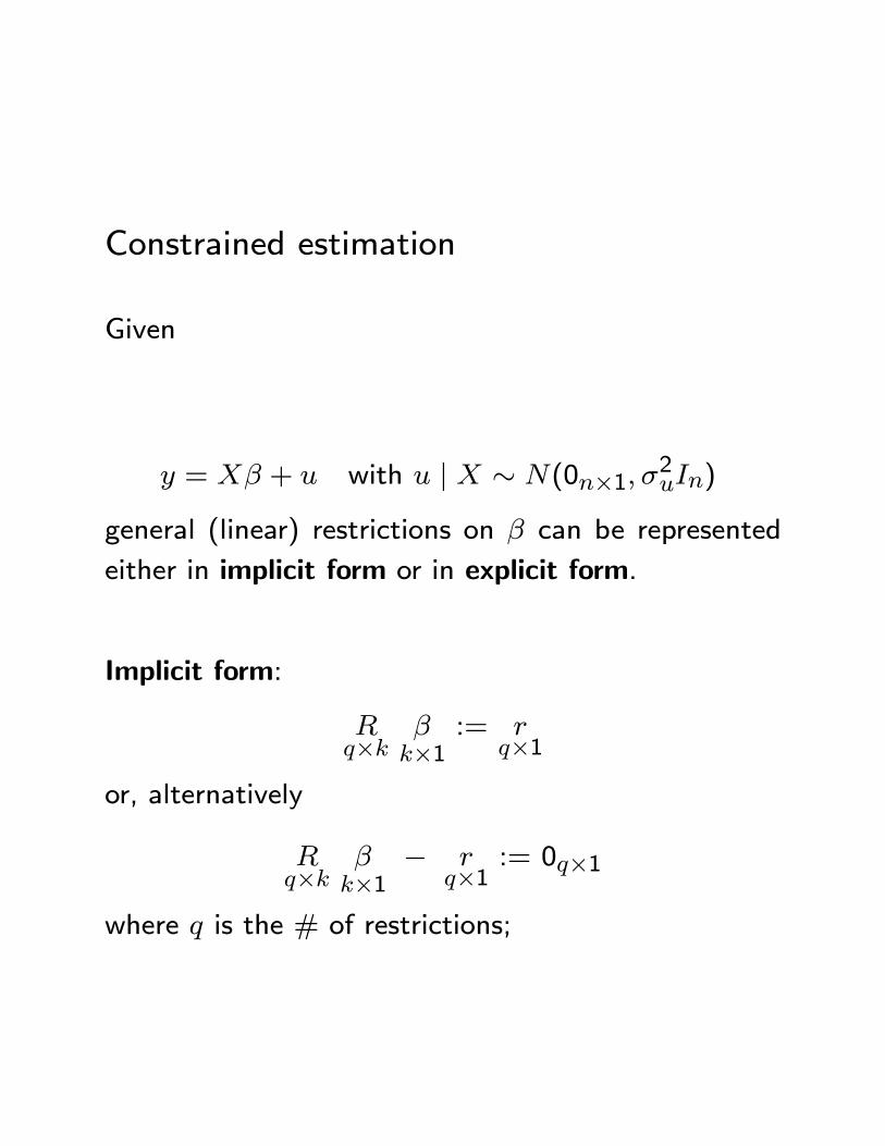
Constrained estimation

Given

y = X� + u with u j X � N(0n�1; �2uIn)

general (linear) restrictions on � can be represented

either in implicit form or in explicit form.

Implicit form:

Rq�k

�k�1

:= rq�1

or, alternatively

Rq�k

�k�1

� rq�1

:= 0q�1

where q is the # of restrictions;

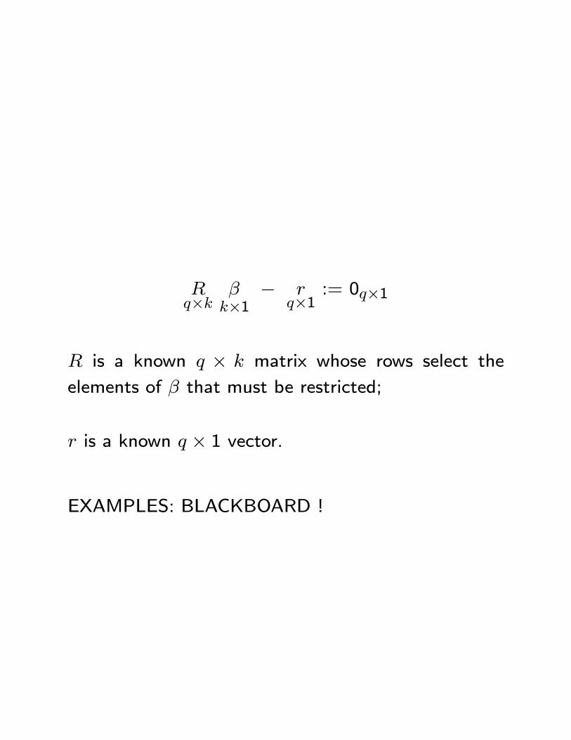
Rq�k

�k�1

� rq�1

:= 0q�1

R is a known q � k matrix whose rows select the

elements of � that must be restricted;

r is a known q � 1 vector.

EXAMPLES: BLACKBOARD !

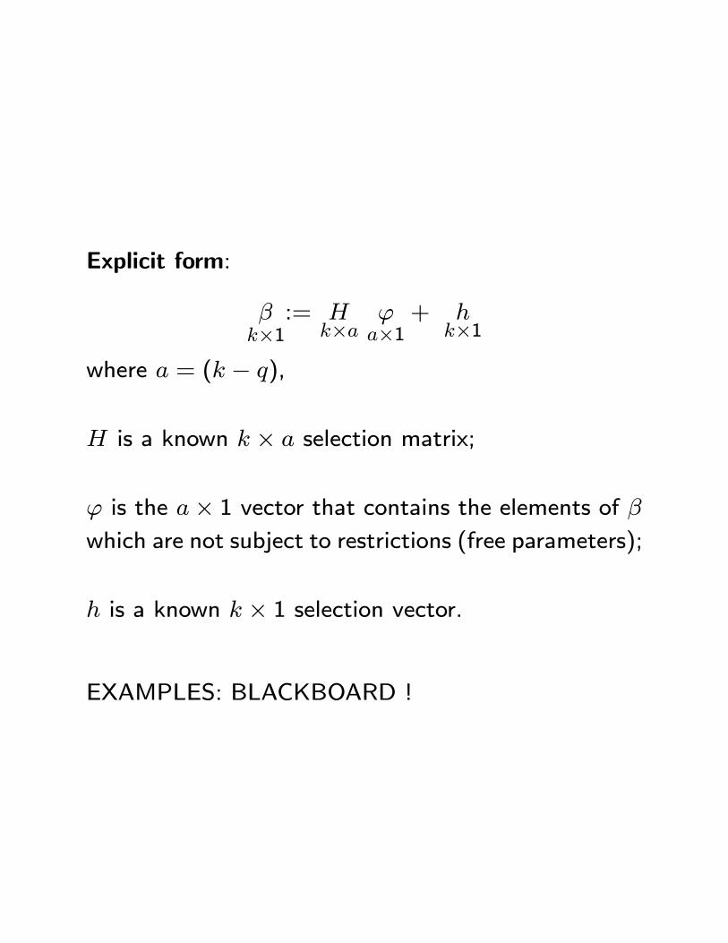
Explicit form:

�k�1

:= Hk�a

'a�1

+ hk�1

where a = (k � q),

H is a known k � a selection matrix;

' is the a� 1 vector that contains the elements of �which are not subject to restrictions (free parameters);

h is a known k � 1 selection vector.

EXAMPLES: BLACKBOARD !

One can write the linear contraints on � either in im-

plicit or in explicit form.

The two methods are alternative but equivalent.

For certain problem it is convenient the implicit form

representation, for others it is convenient the explicit

form representation.

It is therefore clear that there must exist a connection

between the matrices R and H and r and h:

In particular, take the explicit form

�:=H'+ h

and multiply both sides by R, obtaining

R�:=RH'+Rh:

Then, since the right-hand-side of the expression above

must be equal to r, it must hold

RH:=0q�a

Rh:=r:

This means that the (rows of the) matrix R lie in the

null column space of the matrix H

(sp(R) � sp(H?)).

Recall: Let A a n�m matrix, n > m, with (column) rank

m; A = [a1 : a2 : :::: : am].

sp(A) = fall linear combination of a1; a2; :::; amg � Rn

sp(A?) =nv, v0ai = 0; for each i = 1; :::;m

o� Rn

all the vectors in sp(A?) are said to lie in the null column spaceof the matrix A:

LetA? be a n�(n�m) full column rank matrix that satis�es

A0?A = 0(n�m)�mA0A? = 0m�(n�m):

A? is called orthgonal complement of A. The n � n matrix

[A : A?] has rank n and forms a basis of Rn.

Constrained estimation means that one stimates the

model under H0, i.e. imposing the restriction implied

by the null hypothesis.

Suppose that

H0:R�:=r , (H0:�:=H'+ h)

has been accepted by the data.

Then we wish to re-estimate the null model, i.e. the

econometric model that embodies the linear restric-

tion.

In this case, using the restrictions in explicit form is

convenient.

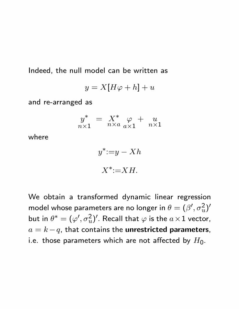
Indeed, the null model can be written as

y = X[H'+ h] + u

and re-arranged as

y�n�1

= X�n�a

'a�1

+ un�1

where

y�:=y �Xh

X�:=XH:

We obtain a transformed dynamic linear regression

model whose parameters are no longer in � = (�0; �2u)0

but in �� = ('0; �2u)0: Recall that ' is the a�1 vector,

a = k�q, that contains the unrestricted parameters,i.e. those parameters which are not a�ected by H0.

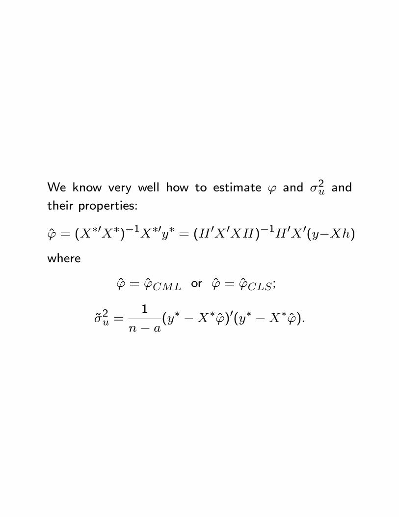
We know very well how to estimate ' and �2u and

their properties:

' = (X�0X�)�1X�0y� = (H 0X 0XH)�1H 0X 0(y�Xh)

where

' = 'CML or ' = 'CLS;

~�2u =1

n� a(y� �X�')0(y� �X�'):

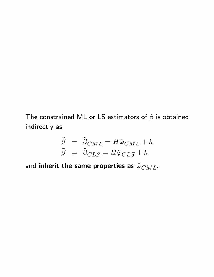
The constrained ML or LS estimators of � is obtained

indirectly as

~� = �CML = H'CML + h

~� = �CLS = H'CLS + h

and inherit the same properties as 'CML.

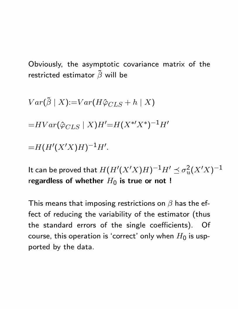
Obviously, the asymptotic covariance matrix of the

restricted estimator ~� will be

V ar(~� j X):=V ar(H'CLS + h j X)

=HV ar('CLS j X)H 0=H(X�0X�)�1H 0

=H(H 0(X 0X)H)�1H 0:

It can be proved thatH(H 0(X 0X)H)�1H 0 � �2u(X0X)�1

regardless of whether H0 is true or not !

This means that imposing restrictions on � has the ef-

fect of reducing the variability of the estimator (thus

the standard errors of the single coe�cients). Of

course, this operation is `correct' only when H0 is usp-

ported by the data.

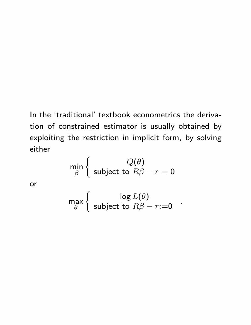
In the `traditional' textbook econometrics the deriva-

tion of constrained estimator is usually obtained by

exploiting the restriction in implicit form, by solving

either

min�

(Q(�)

subject to R� � r = 0

or

max�

(logL(�)

subject to R� � r:=0:

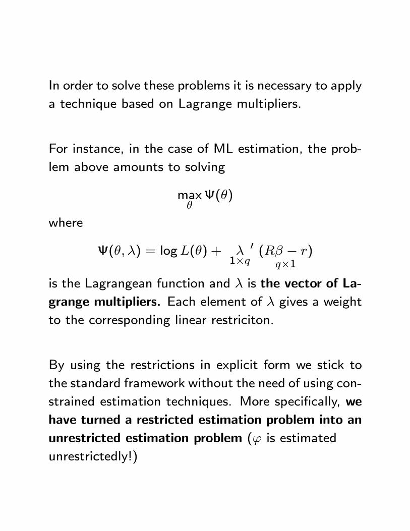
In order to solve these problems it is necessary to apply

a technique based on Lagrange multipliers.

For instance, in the case of ML estimation, the prob-

lem above amounts to solving

max�(�)

where

(�; �) = logL(�) + �1�q

0 (R� � r)q�1

is the Lagrangean function and � is the vector of La-

grange multipliers. Each element of � gives a weight

to the corresponding linear restriciton.

By using the restrictions in explicit form we stick to

the standard framework without the need of using con-

strained estimation techniques. More speci�cally, we

have turned a restricted estimation problem into an

unrestricted estimation problem (' is estimated

unrestrictedly!)

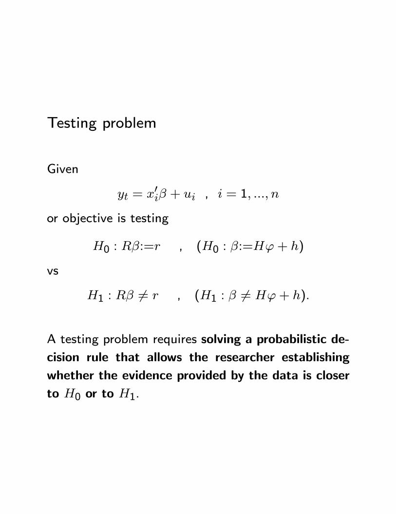
Testing problem

Given

yt = x0i� + ui , i = 1; :::; n

or objective is testing

H0 : R�:=r , (H0 : �:=H'+ h)

vs

H1 : R� 6= r , (H1 : � 6= H'+ h).

A testing problem requires solving a probabilistic de-

cision rule that allows the researcher establishing

whether the evidence provided by the data is closer

to H0 or to H1.

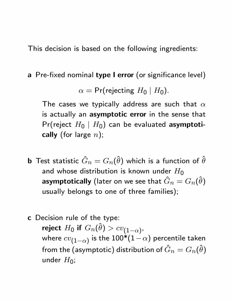
This decision is based on the following ingredients:

a Pre-�xed nominal type I error (or signi�cance level)

� = Pr(rejecting H0 j H0):

The cases we typically address are such that �

is actually an asymptotic error in the sense that

Pr(reject H0 j H0) can be evaluated asymptoti-cally (for large n);

b Test statistic Gn = Gn(�) which is a function of �

and whose distribution is known under H0asymptotically (later on we see that Gn = Gn(�)

usually belongs to one of three families);

c Decision rule of the type:

reject H0 if Gn(�) > cv(1��),where cv(1��) is the 100*(1��) percentile takenfrom the (asymptotic) distribution of Gn = Gn(�)

under H0;

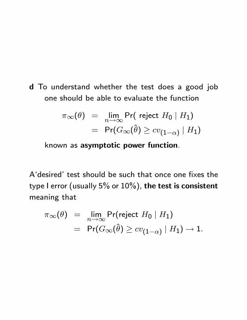
d To understand whether the test does a good job

one should be able to evaluate the function

�1(�) = limn!1Pr( reject H0 j H1)

= Pr(G1(�) � cv(1��) j H1)

known as asymptotic power function.

A`desired' test should be such that once one �xes the

type I error (usually 5% or 10%), the test is consistent

meaning that

�1(�) = limn!1Pr(reject H0 j H1)

= Pr(G1(�) � cv(1��) j H1)! 1:

When estimation is perfomed with ML we can clas-

sify the test statistic Gn = Gn(�) into three families,

known as Wald, Lagrange Multipliers (LM) and Like-

lihood Ratio (LR) tests.

However, the existence of these three families is not

solely con�ned to ML estimation but can be extended

to other classes of estimators as well.

General philosophy:

Wald These type of tests are based on the idea of

checking whether the unrestricted (ML) estimator

of � (i.e. the estimator obtained without impos-

ing any constraint) is `close in a statistical sense'

to H0, namely whether

R� � r � 0q�1which is what one would expect if H0 is true.

Computing a Wald-type test requires estimat-

ing the regression model one time without any

restriction.

LM These type of tests are based on the the estima-

tion of the null model (i.e. the regression model

under H0), hence are based on the constrained

estimator of �. Let � be the unconstrained (ob-

tained under H1) estimator of � and ~� its con-

strained (obtained under H0) counterpart. The

idea is that if H0 is true, the score of the unre-

stricted model, evaluated at the constrained esti-

mator (recall that sn(�) = 0k�1) should be `closeto zero in a statistical sense', i.e.

sn(~�) � 0k�1:

Computing a LM test requires estimating the

regression model one time under the restrictions

implied by H0 (however, it also requires that we

know the structure of the score of the unrestricted

model !).

LR The type of tests are based on the idea of estimat-

ing the linear regression model both under H0(~�) and without restrictions (�); estimation is

carried out two times. If H0 is true, the distance

between the likelihood functions of the null and

unrestricted models should not be too large (note

that one always has logL(~�) � logL(�)).

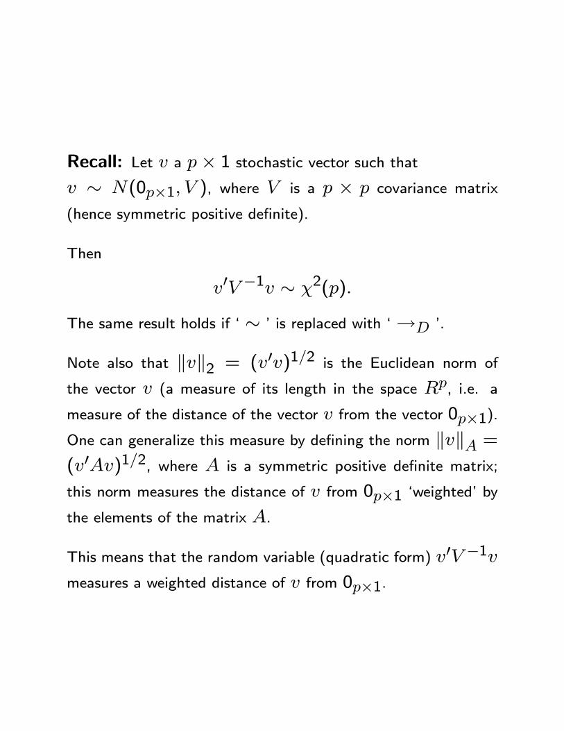
Recall: Let v a p� 1 stochastic vector such thatv � N(0p�1; V ), where V is a p � p covariance matrix

(hence symmetric positive de�nite).

Then

v0V �1v � �2(p):

The same result holds if ` � ' is replaced with `!D '.

Note also that kvk2 = (v0v)1=2 is the Euclidean norm of

the vector v (a measure of its length in the space Rp, i.e. a

measure of the distance of the vector v from the vector 0p�1).One can generalize this measure by de�ning the norm kvkA =(v0Av)1=2, where A is a symmetric positive de�nite matrix;

this norm measures the distance of v from 0p�1 `weighted' bythe elements of the matrix A.

This means that the random variable (quadratic form) v0V �1vmeasures a weighted distance of v from 0p�1.

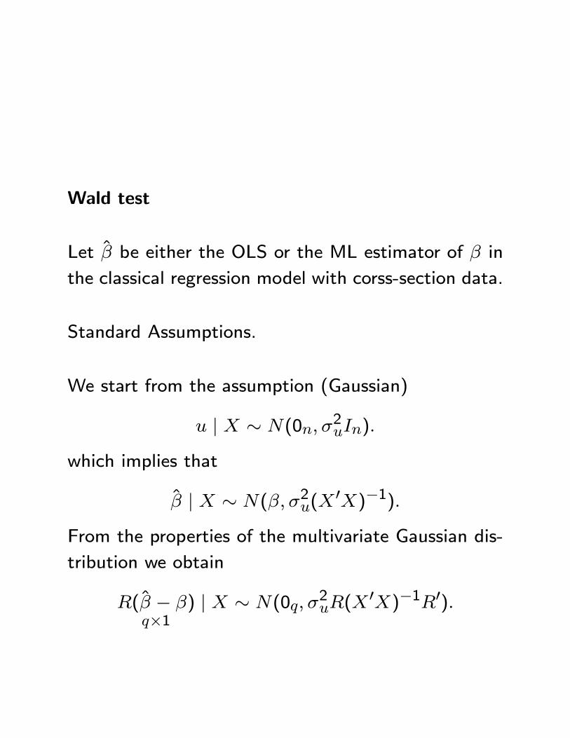
Wald test

Let � be either the OLS or the ML estimator of � in

the classical regression model with corss-section data.

Standard Assumptions.

We start from the assumption (Gaussian)

u j X � N(0n; �2uIn):

which implies that

� j X � N(�; �2u(X0X)�1):

From the properties of the multivariate Gaussian dis-

tribution we obtain

R(� � �)q�1

j X � N(0q; �2uR(X

0X)�1R0):

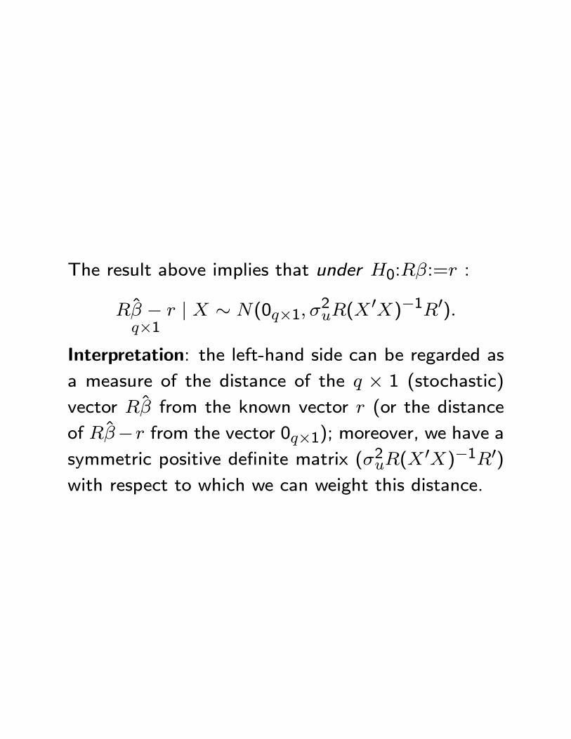
The result above implies that under H0:R�:=r :

R� � rq�1

j X � N(0q�1; �2uR(X

0X)�1R0):

Interpretation: the left-hand side can be regarded as

a measure of the distance of the q � 1 (stochastic)

vector R� from the known vector r (or the distance

of R��r from the vector 0q�1); moreover, we have asymmetric positive de�nite matrix (�2uR(X

0X)�1R0)with respect to which we can weight this distance.

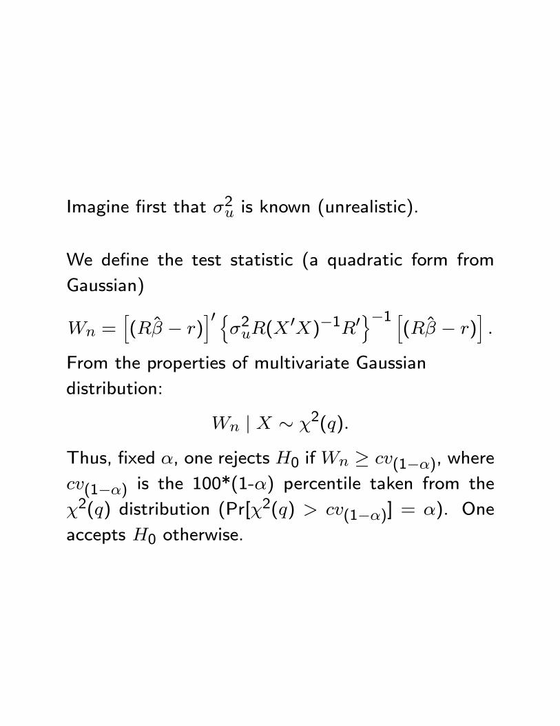
Imagine �rst that �2u is known (unrealistic).

We de�ne the test statistic (a quadratic form from

Gaussian)

Wn =h(R� � r)

i0 n�2uR(X

0X)�1R0o�1 h

(R� � r)i:

From the properties of multivariate Gaussian

distribution:

Wn j X � �2(q):

Thus, �xed �, one rejects H0 ifWn � cv(1��), wherecv(1��) is the 100*(1-�) percentile taken from the

�2(q) distribution (Pr[�2(q) > cv(1��)] = �). One

accepts H0 otherwise.

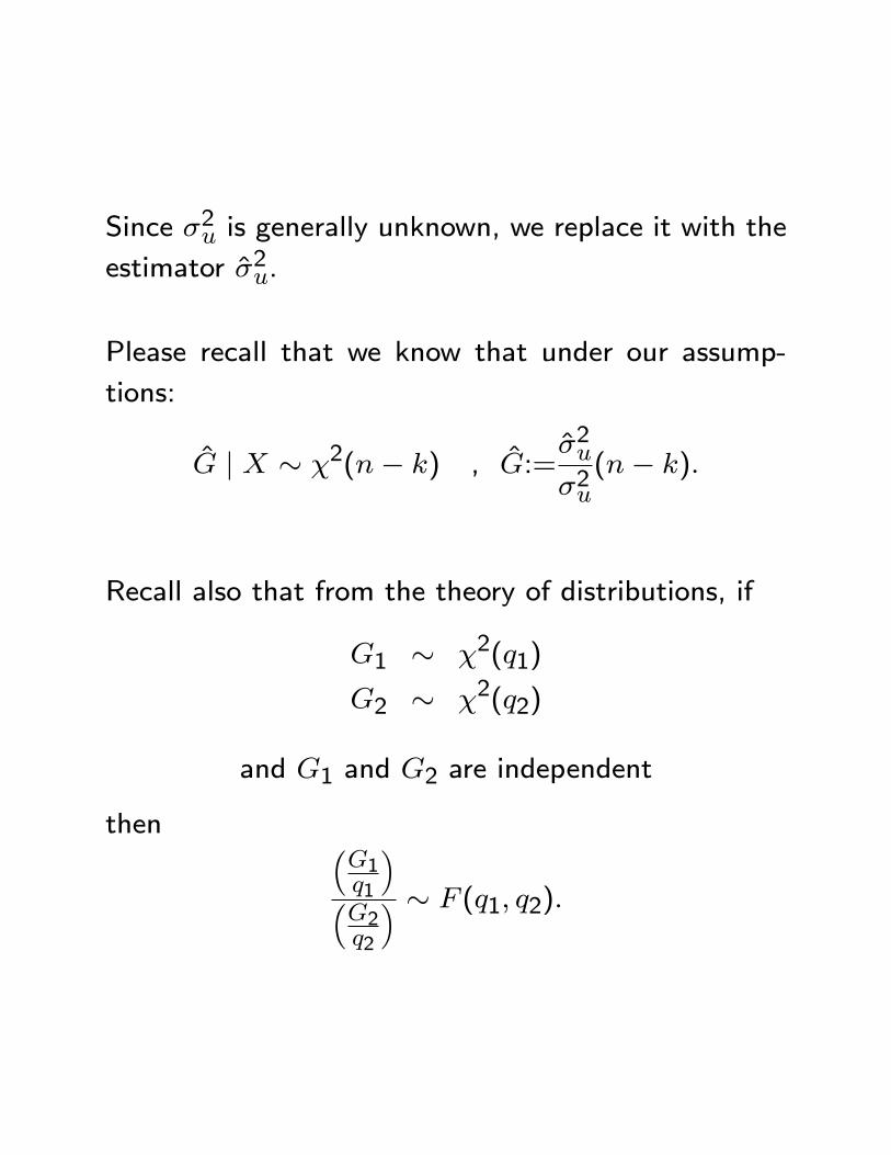
Since �2u is generally unknown, we replace it with the

estimator �2u.

Please recall that we know that under our assump-

tions:

G j X � �2(n� k) , G:=�2u�2u(n� k):

Recall also that from the theory of distributions, if

G1 � �2(q1)

G2 � �2(q2)

and G1 and G2 are independent

then �G1q1

��G2q2

� � F (q1; q2):

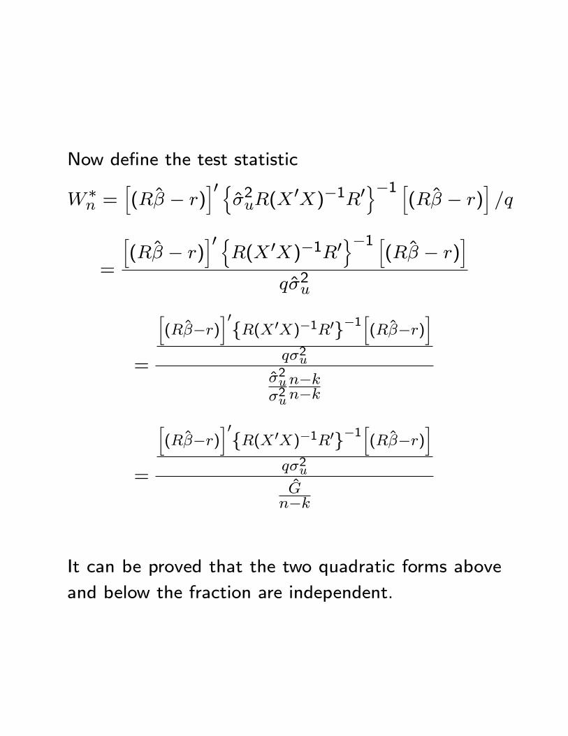
Now de�ne the test statistic

W �n =

h(R� � r)

i0 n�2uR(X

0X)�1R0o�1 h

(R� � r)i=q

=

h(R� � r)

i0 nR(X 0X)�1R0

o�1 h(R� � r)

iq�2u

=

h(R��r)

i0fR(X 0X)�1R0g�1

h(R��r)

iq�2u

�2u�2u

n�kn�k

=

h(R��r)

i0fR(X 0X)�1R0g�1

h(R��r)

iq�2uGn�k

It can be proved that the two quadratic forms above

and below the fraction are independent.

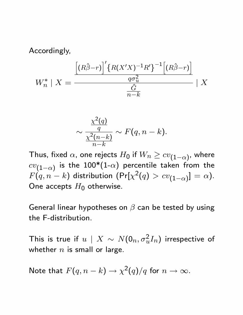
Accordingly,

W �n j X =

h(R��r)

i0fR(X 0X)�1R0g�1

h(R��r)

iq�2uGn�k

j X

��2(q)q

�2(n�k)n�k

� F (q; n� k):

Thus, �xed �, one rejects H0 ifWn � cv(1��), wherecv(1��) is the 100*(1-�) percentile taken from the

F (q; n � k) distribution (Pr[�2(q) > cv(1��)] = �).

One accepts H0 otherwise.

General linear hypotheses on � can be tested by using

the F-distribution.

This is true if u j X � N(0n; �2uIn) irrespective of

whether n is small or large.

Note that F (q; n� k)! �2(q)=q for n!1:

LM and LR tests will be reviewed when we deal with

the regression model based on time series data.