An Equational Approach to Secure Multi-party Computation∗

Daniele Micciancio† Stefano Tessaro‡

January 12, 2013

Abstract

We present a novel framework for the description and analysis of secure computation proto-cols that is at the same time mathematically rigorous and notationally lightweight and concise.The distinguishing feature of the framework is that it allows to specify (and analyze) protocolsin a manner that is largely independent of time, greatly simplifying the study of cryptographicprotocols. At the notational level, protocols are described by systems of mathematical equations(over domains), and can be studied through simple algebraic manipulations like substitutionsand variable elimination. We exemplify our framework by analyzing in detail two classic pro-tocols: a protocol for secure broadcast, and a verifiable secret sharing protocol, the second ofwhich illustrates the ability of our framework to deal with probabilistic systems, still in a purelyequational way.

1 Introduction

Secure multiparty computation (MPC) is a cornerstone of theoretical cryptography, and a problemthat is attracting increasingly more attention in practice too due to the pervasive use of distributedapplications over the Internet and the growing popularity of computation outsourcing. The areahas a long history, dating back to the seminal work of Yao [29] in the early 1980s, and a steadyflow of papers contributing extensions and improvements that lasts to the present day (startingwith the seminal works [12, 6, 3] introducing general protocols, and followed by literally hundreds ofpapers). But it is fair to say that MPC has yet to deliver its full load of potential benefits both to theapplied and theoretical cryptography research communities. In fact, large portions of the researchcommunity still see MPC as a highly specialized research area, where only the top experts canread and fully understand the highly technical research papers routinely published in mainstreamcrypto conferences. Two main obstacles have kept, so far, MPC from becoming a more widespreadtool to be used both in theoretical and applied cryptography: the prohibitive computational costof executing many MPC protocols, and the inherent complexity of the models used to describethe protocols themselves. Much progress has been made in improving the efficiency of the first

∗An edited version of this work appears in the proceedings of Innovations in Theoretical Computer Science,ITCS 2013. This is the authors’ copy. This material is based on research sponsored by DARPA under agreementnumber FA8750-11-C-0096. The U.S. Government is authorized to reproduce and distribute reprints for Governmentalpurposes notwithstanding any copyright notation thereon. The views and conclusions contained herein are those ofthe authors and should not be interpreted as necessarily representing the official policies or endorsements, eitherexpressed or implied, of DARPA or the U.S. Government.†University of California, San Diego. daniele@cs.ucsd.edu.‡Massachusetts Institute of Technology. tessaro@csail.mit.edu

1

protocols [29, 12, 6] in a variety of models and with respect to several complexity measures, evenleading to concrete implementations (cf. e.g. [19, 4, 17, 7, 24, 11]). However, the underlying modelsto describe and analyze security properties are still rather complex.

What makes MPC harder to model than traditional cryptographic primitives like encryption,is the inherently distributed nature of the security task being addressed: there are several distinctand mutually distrustful parties trying to perform a joint computation, in such a way that even ifsome parties deviate from the protocol, the protocol still executes in a robust and secure way.

The difficulty of properly modeling secure distributed computation is well recognized within thecryptographic community, and documented by several definitional papers attempting to improvethe current state of the art [22, 9, 10, 23, 2, 18, 15].Unfortunately, the current state of the art is stillpretty sore, with definitional/modeling papers easily reaching encyclopedic page counts, setting avery high barrier of entry for most cryptographers to contribute or actively follow the develop-ments in MPC research. Moreover, most MPC papers are written in a semi-formal style reflectingan uncomfortable trade-off between the desire of giving to the subject the rigorous treatment itdeserves and the implicit acknowledgment that this is just not feasible using the currently availableformalisms (and even more so, within the page constraints of a typical conference or even journalpublication.) The goal of this paper is to drastically change this state of affairs, by putting forwarda model for the study of MPC protocols that is both concise, rigorous, and still firmly rooted inthe intuitive ideas that pervade most past work on secure computation and most cryptographersknow and love.

An interesting line of work, with goals similar to ours, is described in a recent paper of Mauerand Renner [20]. The works share the common goal of providing a simpler and mathematicallyrigorous framework for studying cryptographic protocols, but are fundamentally different. Themain difference between [20] and our work is that [20] adopts an axiomatic approach (postulatingthat abstract cryptographic objects satisfy certain natural and desirable properties), while ourline of work is model theoretic, offering a (high level, but) concrete model of computation wherecryptographic protocols can be directly described by standard mathematical objects. The twoapproaches are complementary, as the computational model described in this paper satisfies all thenatural and desirable properties postulated in [20]. So, one may use the axiomatic framework of[20] to prove some of the properties of protocols specified in our model. It would be interesting torefine the set of axioms proposed in [20] into a sound and complete axiomatization of the modeldescribed in this work, in order to show that the two frameworks are equally powerful.

1.1 The simulation paradigm

Let us recall the well known and established simulation paradigm that underlies essentially allMPC security definitions. Cryptographic protocols are typically described by several componentprograms P1, . . . , Pn executed by n participating parties, interconnected by a communication net-work N , and usually rendered by a diagram similar to the one in Figure 1 (left): each party receivessome input xi from an external environment, and sends/receives messages si, ri from the network.Based on the external inputs xi, and the messages si, ri transmitted over the network N , each partyproduces some output value yi which is returned to the outside world as the visible output of run-ning the protocol. The computational task that the protocol is trying to implement is described bya single monolithic program F , called the “ideal functionality”, which has the same input/outputinterface as the system consisting of P1, . . . , Pn and N , as shown in Figure 1 (right). Conceptually,F is executed by a centralized entity that interacts with the individual parties through their local

2

N

P1

r1s1

yixi

P2

r2s2

yixi

P3

r3s3

yixi

P4

r4s4

yixi

F

y1x1 y2x2 y3x3 y4x4

Figure 1: A multiparty protocol P1, . . . , P4 with communication network N (left) implementing afunctionality F (right).

N

P1

r1s1

yixi

P2

r2s2

yixi

r3s3 r4s4

F

S

y3x3

risi

y4x4

risi

y1x1 y2x2

Figure 2: Simulation based security. The protocol P1, . . . , P4 is a secure implementation of func-tionality F if the system (left) exposed to an adversary that corrupts a subset of parties (say P3

and P4) is indistinguishable from the one system (right) recreated by a simulator S interacting withF .

input/output interfaces xi/yi, and processes the data in a prescribed and trustworthy manner. Aprotocol P1, . . . , Pn correctly implements functionality F in the communication model provided byN if the two systems depicted in Figure 1 (left and right) exhibit the same input/output behavior.

Of course, this is not enough for the protocol to be secure. In a cryptographic context, someparties can get corrupted, in which case an adversary (modeled as part of the external executionenvironment) gains direct access to the parties’ communication channels si, ri and is not bound tofollow the instructions of the protocol programs Pi. Figure 2 (left) shows an execution where P3

and P4 are corrupted. The simulation paradigm postulates that whatever can be achieved by aconcrete adversary attacking the protocol, can also be achieved by an idealized adversary S (calledthe simulator) attacking the ideal functionality F . In Figure 2 (right), the simulator takes over therole of P3 and P4, communicating for them with the ideal functionality, and recreating the attack ofa real adversary by emulating an interface that exposes the network communication channels of P3

and P4. The protocol P1, . . . , Pn securely implements functionality F if the systems described onthe left and right of Figure 2 are functionally equivalent: no adversary (environment) connecting

3

to the external channels x1, y1, x2, y2, s3, r3, s4, r4 can (efficiently) determine if it is interacting withthe system described in Figure 2 (left) or the one in Figure 2 (right). In other words, anythingthat can be achieved corrupting a set of parties in a real protocol execution, can also be emulatedby corrupting the same set of parties in an idealized execution where the protocol functionality Fis executed by a trusted party in a perfectly secure manner.

This is a very powerful idea, inspired by the seminal work on zero knowledge proof systems [13],and embodied in many subsequent papers about MPC. But, of course, as much as evocative thediagrams in Figure 2 may be, they fall short of providing a formal definition of security. In fact,a similar picture can be drawn to describe essentially any of the secure multiparty computationmodels proposed so far at a very abstract level, but the real work is in the definition of whatthe blocks and communication links connecting them actually represent. Traditionally, buildingon classical work from computational complexity on interactive proof systems, MPC is formalizedby modeling each block by an interactive Turing machine (ITM), a venerable model of sequentialcomputation extended with some “communication tapes” used to model the channels connectingthe various blocks. Unfortunately, this only provides an adequate model for the local computationperformed by each component block, leaving out the most interesting features that distinguish MPCfrom simpler cryptographic tasks: computation is distributed and the concurrent execution of allITMs needs to be carefully orchestrated. In a synchronous communication environment, wherelocal computations proceed in lockstep through a sequence of rounds, and messages are exchangedonly between rounds, this is relatively easy. But in asynchronous communication environments likethe Internet, dealing with concurrency is a much trickier business. The standard approach to dealwith concurrency in asynchronous distributed systems is to use nondeterminism: a system does notdescribe a single behavior, but a set of possible behaviors corresponding to all possible interleavingsand message delivery orders. But nondeterminism is largely incompatible with cryptography, as itallows to break any cryptographic function by nondeterministically guessing the value of a secretkey. As a result, cryptographic models of concurrent execution resort to an adversarially andadaptively chosen, but deterministic, message delivery order: whenever a message is scheduled fortransmission between two component, it is simply queued and an external scheduling unit (which isalso modeled as part of the environment) is notified about the event. While providing a technicallysound escape route from the dangers of mixing nondeterministic concurrency with cryptography,this approach has several shortcomings:

- Adding a scheduler further increases the complexity of the system, making simulation basedproofs of security even more technical.

- It results in a system that in many respects seems overspecified: as the goal is to design arobust system that exhibits the prescribed behavior in any execution environment, it wouldseem more desirable to abstract the scheduling away, rather than specifying it in every singledetail of a fully sequential ordering of events.

- Finally, the intuitive and appealing idea conveyed by the diagrams in Figure 2 is in a senselost, as the system is now more accurately described by a collection of isolated componentsall connected exclusively to the external environment that orchestrates their executions byscheduling the messages.

4

F

Q1

y1x1

wizi

Q2

y2x2

wizi

y3x3 y4x4

G

S′

w3z3

yixi

w4z4

yixi

w1z1 w2z2

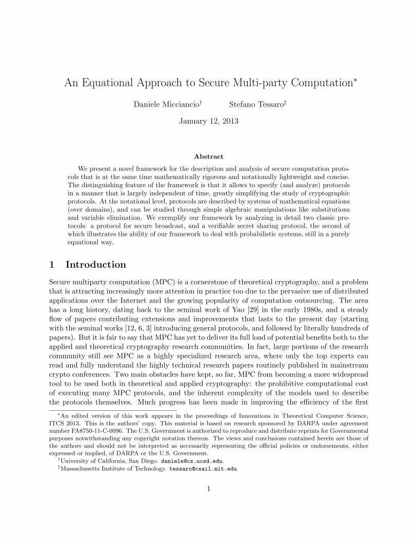
Figure 3: A protocol Qi implementing G in the F -hybrid model.

1.2 Our work

In this paper we describe a model of distributed computation that retains the simplicity andintuitiveness conveyed by the diagrams in Figures 1 and 2, and still it is both mathematicallyrigorous and concise. In other words, we seek a model where the components Pi, N, F, S occurringin the description and analysis of a protocol, and the systems obtained interconnecting them, canbe given a simple and precise mathematical meaning. The operation of composing systems togethershould also be well defined, and satisfy a number of useful and intuitive properties, e.g., the resultof connecting several blocks together does not depend on the order in which the connections aremade. (Just as we expect the meaning of a diagram to be independent of the order in which thediagram was drawn.) Finally, it should provide a solid foundation for equational reasoning, in thesense that equivalent systems can be replaced by equivalent systems in any context.

Within such a framework, the proof that protocols can be composed together should be as simpleas the following informal argument. (In fact, given the model formally defined in the rest of thepaper, the following is actually a rigorous proof that our definition satisfies a universal composabilityproperty.) Say we have a protocol P1, . . . , Pn securely implementing ideal functionality F using acommunication network N , and also a protocol Q1, . . . , Qn in the F -hybrid model (i.e., an idealizedmodel where parties can interact through functionality F ) that securely implements functionalityG. The security of the second protocol is illustrated in Figure 3.

Then, the protocol obtained simply by connecting Pi and Qi together is a secure implementationof G, in the standard communication model N . Moreover, the simulator showing that the composedprotocol is secure is easily obtained simply by composing the simulators for the two componentprotocols. In other words, we want to show that an adversary attacking the real system describedin Figure 4 (left) is equivalent to the composition of the simulators attacking the ideal functionalityG as described in Figure 4 (right).

This is easily shown by transforming Figure 4 (left) to Figure 4 (right) in two steps, goingthrough the hybrid system described in Figure 5. Specifically, first we use the security of Pi toreplace the system described in Figure 2 (left) with the one in Figure 2 (right). This turns thesystem in Figure 4 (left) into the equivalent one in Figure 5. Next we use the security of Qi tosubstitute the system in Figure 3 (left) with the one in Figure 3 (right). This turns Figure 5 intoFigure 4 (right).

While the framework proposed in this paper allows to work with complex distributed systems

5

N

P1

Q1

r1s1

yixi

wizi

P2

Q2

r2s2

yixi

wizi

r3s3 r4s4

G

S′

S

w3z3

xi yi

si ri

w4z4

xi yi

si ri

w1z1 w2z2

Figure 4: Protocol composition. Security is proved using a hybrid argument.

F

SQ1

y1x1

wizi

Q2

y2x2

wizi

y3x3

risi

y4x4

risi

Figure 5: Hybrid system to prove the security of the composed protocol

6

with the same simplicity as the informal reasoning described in this section, it is quite powerful andflexible. For example, it allows to model not only protocols that are universally composable, butalso protocols that retain their security only when used in restricted contexts. For simplicity, in thispaper we focus on perfectly secure protocols against unbounded adversaries, as this already allowsus to describe interesting protocols that illustrate the most important feature of our framework:the ability to design and analyze protocols without explicitly resorting to the notion of time andsequential scheduling of messages. Moreover, within the framework of universally composability,it is quite common to design perfectly secure protocols in a hybrid model that offers idealizedversions of the cryptographic primitives, and then resorting to computationally secure cryptographicprimitives only to realize the hybrid model. So, a good model for the analysis of perfect or statisticalsecurity can already be a useful and usable aid for the design of more general computationally secureprotocols. Natively extending our framework to statistically or computationally secure protocols isalso an attractive possibility. We consider the perfect/statistical/computational security dimensionas being mostly orthogonal to the issues dealt with in this paper, and we believe the model describedhere offers a solid basis for extensions in that direction.

1.3 Techniques

In order to realize our vision, we introduce a computational model in which security proofs canbe carried out without explicitly dealing with the notion of time. Formally, we associate to eachcommunication channel connecting two components the set of all possible “channel histories”,partially ordered according to their information content or temporal ordering. The simplest exampleis the set of all finite sequences M∗ of messages from some underlying message space, orderedaccording to the prefix ordering relation. The components of the system are then modeled asfunctions mapping input histories to output histories. The functions are subject to some naturalconditions, e.g., monotonicity: receiving more input values can only results in more output valuesbeing produced. Under appropriate technical conditions on the ordered sets associated to thecommunication channels, and the functions modeling the computations performed by the systemcomponents, this results in a well behaved framework, where components can be connected together,even forming loops, and always resulting in a unique and well defined function describing theinput/output behavior of the whole system. Previous approaches to model interactive systems,such as Kahn networks [16] and Maurer’s random systems [21], can indeed be seen as special casesof our general process model.1 The resulting model is quite powerful, allowing even to modelprobabilistic computation as a special case. However, the simplicity of the model has a price: allcomponents of the system must be monotone with respect to the information ordering relation. Forexample, if a program P on input messages x1, x2 outputs P (x1, x2) = (y1, y2, y3), then on inputx1, x2, x3 it can only output a sequence of messages that extends (y1, y2, y3) with more output.In other words, P cannot “go back in time” and change y1, y2, y3. While this is a very naturaland seemingly innocuous restriction, it also means that the program run by P cannot performoperations of the form “if no input message has been received yet, then send y”. This is because ifan input message is received at a later point, P cannot go back in time and not send y.

1For the readers well versed in the subject, we remark that our model can be regarded as a generalization ofKahn networks where the channel behaviors are elements of arbitrary partially ordered sets (or, more precisely,domains) rather than simple sequences of messages. This is a significant generalization that allows to deal withprobabilistic computations and intrinsically nondeterministic systems seamlessly, without incurring into the Brock-Ackerman anomaly and similar problems.

7

It is our thesis that these time dependent operations make cryptographic protocols harder tounderstand and analyze, and therefore should be avoided whenever possible.

Organization. The rest of the paper is organized as follows. In Section 2 we present our frame-work for the description and analysis of concurrent processes, and illustrate the definitions using atoy example. Next, we demonstrate the applicability of the framework by carefully describing andanalyzing two classic cryptographic protocols: secure broadcast (in Section 3) and verifiable secretsharing (in Section 4). The secure broadcast protocol in Section 3 is essentially the one of Bracha,and only uses deterministic functions. Our modular analysis of the protocol illustrates the use ofsubprotocols that are not universally composable. The verifiable secret sharing protocol analyzedin Section 4 provides an example of randomized protocol.

2 Distributed Systems, Composition, and Secure Computation

In this section we introduce our mathematical framework for the description and analysis of dis-tributed systems. We start with a high level description of our approach, which will be sufficientto apply our framework and to follow the proofs. We then give more foundational details justifyingsoundness of our approach. Finally, we provide security definitions for protocols in our framework.

2.1 Processes and systems

Introducing processes: An example and notational conventions. Our framework models(asynchronous and reactive) processes and systems with one or more input and output channelsas mathematical functions mapping input histories to output histories. Before introducing moreformal definitions, let us illustrate this concept with a simple example. Consider a deterministicprocess with one input and one output channels, which receives as input a sequence of messages,x[1], . . . , x[k], where each x[k] is (or can be parsed as) an integer. The process receives the messagessequentially, one at a time, and in order to make the process finite one may assume that the processwill accept only the first n messages. Upon receiving each input message x[i], the process incrementsthe value and immediately outputs x[i]+1. It is not hard to model the process in terms of a functionmapping input to output sequences: The input and output of the function modeling the process arethe set Z≤n of integer sequences of length at most n, and the process is described by the functionF: Z≤n → Z≤n mapping each input sequence x ∈ Zk (for some k ≤ n) to the output sequencey ∈ Zk of the same length defined by the equations y[i] = x[i] + 1 (for i = 1, . . . , k). There aremultiple ways one can possibly describe such a function. We describe the process in equationalform as in Figure 6 (left). In the example, the first line assigns names to the function, inputand output variables, while the remaining lines are equations that define the value of the outputvariables in terms of the input variables. Each variable ranges over a specific set (x, y ∈ Z≤n), butfor simplicity we often leave the specification of this set implicit, as it is usually clear from thecontext. By convention, all variables that appear in the equations, but not as part of the inputor output variables, are considered local/internal variables, whose only purpose is to help definingthe value of the output variables in terms of the input variables. Free index variables (e.g., i, j)are universally quantified (over appropriate ranges) and used to compactly describe sets of similarequations.

8

F(x) = y:y[i] = x[i]+1 (i = 1, . . . , |x|)

G(y) = (z, w):z = yw = y

H(z) = x:x[1] = 1x[j + 1] = z[j] (j ≤ min{|z|, n− 1})

Figure 6: Some simple processes

Processes as monotone functions. In general, the reason we define a process F as a functionmapping sequences to sequences2 (rather than, say, as a function f(x) = x + 1 applied to eachincoming message x) is that it allows to describe the most general type of (e.g., stateful, reactive)process, whose output is a function of all messages received as input during the execution of theprotocol. (Note that we do not need to model state explicitly.) Also, such functions can describeprocesses with multiple input and output channels by letting inputs and outputs be tuples ofmessage sequences. However, clearly, not any such function mapping input to output sequencescan be a valid process. To capture valid functions representing a process, input and output sets areendowed with a partial ordering relation ≤, where x ≤ y means that y is a possible future of x. (Inthe case of sequences of messages, ≤ is the standard prefix partial ordering relation, where x ≤ y ify = x|z for some other sequence z, and x|z is the concatenation of the two sequences.) Functionsdescribing processes should be naturally restricted to monotone functions, i.e., functions such thatx ≤ y implies F(x) ≤ F(y). In our example, this simply means that if on input a sequence ofmessages x, F(x) is produced as output, upon receiving additional messages z, the output sequencecan only get longer, i.e., F(y) = F(x|z) = F(x)|z′ for some z′. In other words, once the messagesF(x) are sent out, the process cannot change its mind and set the output to a sequence that doesnot start with F(x).

Note that so far we only discussed an example of a deterministic process. Below, after intro-ducing some further foundational tools, we will see that probabilistic processes are captured inthe same way by letting the function output be a distribution over sequences, rather than a singlesequence of symbols.

Further examples and notational conventions. In the examples, |x| denotes the length of asequence x, and we use array notation x[i] to index the elements of a sequence. Figure 6 gives twomore examples of processes that further illustrate notational conventions. Process G, in Figure 6(middle), simply duplicates the input y (as usual in Z≤n) and copies the input messages to twodifferent output channels z and w. When input or output values are tuples, we usually give separatenames to each component of the tuple. As before, all variables take values in Z≤n and the outputvalues are defined by a set of equations that express the output in terms of the input. Finally,process H(z) takes as input a sequence z ∈ Z≤n, and outputs the message 1 followed by themessages z received as input, possibly truncated to a prefix z[< n] of length at most n− 1, so thatthe output sequence x has length at most n.

Process composition. Processes are composed in the expected way, connecting some outputvariables to other input variables. Here we use the convention that variable names are used to

2Here we use sequences just as a concrete example. Our framework uses more general structures, namely domains.

9

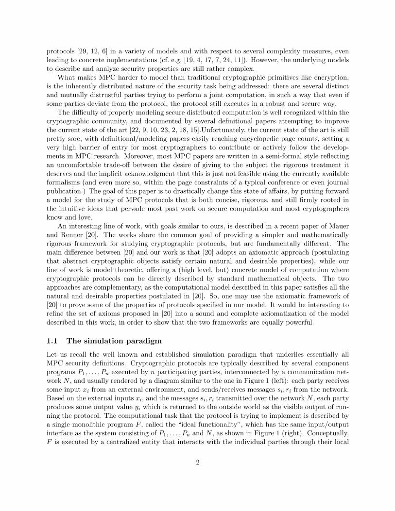
[G | H](y) = (w, x):z = yw = yx[1] = 1x[j + 1] = z[j] (j < n)

[G | H](y) = (w, x):w = yx[1] = 1x[j + 1] = y[j] (j < n)

Figure 7: Process composition

implicitly specify how different processes are meant to be connected together.3 Composing twoprocesses together yields, in turn, another process, which is obtained simply combining all theequations. We often refer to the resulting process as a system to stress its structure as a compositionof basic processes. However, it should be noted that both a process and a system are objects ofthe same mathematical type, namely monotone functions described by systems of equations. Forexample, the result of composing G and H from Figure 6 yields the process (G | H) shown in Figure 7(left), with input y and output (w, x), where w = y replicates the input to make it externallyvisible. We use the convention that by default processes are connected by private channels, notvisible outside of the system. This is modeled by turning their common input/output variablesinto local ones, not part of the input or output of the composed system. Of course, one can alwayseither override this convention by explicitly listing such common input/output variables as part ofthe output, or bypass it by duplicating the value of a variable as done for example by process G.This is just a syntactical convention, and several other choices are possible, including never hidingvariables during process composition and introducing a special projection operator to hide internalvariables.

Since processes formally define functions (from input to output variables), and equations are justa syntactic method to specify functions, equations can be simplified without affecting the process.Simplifications are easily performed by substitution and variable elimination. For example, usingthe first equation z = y, one can substitute y for z, turning the last equation in the system intox[i + 1] = y[i]. At this point, the local variable z is no longer used anywhere, and its definingequation can be removed from the system. The result is shown in Figure 7 (right). We remarkthat the two systems of equations shown in Figure 7 define the same process: they have the sameinput and output variables, and the equations define precisely the same function.

Feedback loops and recursive equations. Now consider the composition of all three processesF,G,H from Figure 6. Composition can be performed one pair at a time, and in any order, e.g.,as [[F | G] | H] or [F | [G | H]]. Given the appropriate mathematical definitions, it can be easilyshown that the result is the same, independent from the order of composition. (This is clear atthe syntactic level, where process composition is simply defined by combining all the equationstogether. But associativity of composition can also be proved at the semantic level, where theobjects being combined are functions.) So, we write [F | G | H] to denote the result of composingmultiple processes together, shown in Figure 8 (left). When studying multi-party computationprotocols, one is naturally led to consider collections of processes, e.g., P1, . . . ,Pn, correspondingto the individual programs run by each participant. Given a collection {Pi}i and a subset of indices

3We stress that this is just a notational convention, and there are many other syntactical mechanisms that can beused to specify the “wiring” in more or less explicit ways.

10

[F | G | H]() = w:y[i] = x[i] + 1 (i ≤ n)z = yw = yx[1] = 1x[j + 1] = z[j] (j < n)

[F | G | H]() = w:w[1] = 2w[j + 1] = w[j] + 1 (j < n)

Figure 8: Example of recursive process

I ⊆ {1, . . . , n}, we write PI to denote the composition of all Pi with i ∈ I. Similarly, we use xA orx[A] to denote a vector indexed by i ∈ A. As a matter of notation, we also use xA to denote the|A|-dimensional vector indexed by i ∈ A with all components set equal to x.

The system [F | G | H] has no inputs, and only one output w. More interestingly, the result ofcomposing all three processes yields a recursive system of equations, where y is a function of x, x isa function of z and z is a function of y. Before worrying about solving the recursion, we can simplifythe system. A few substitutions and variable eliminations yield the system in Figure 8 (right). Thesystem consists of a single, recursively defined output variable w. The recursive definition of w iseasy to solve, yielding w[i] = i+ 1 for i ≤ n.

2.2 Foundations: Domain theory and probabilistic processes

So far, equations have been treated in an intuitive and semi-formal way, and in fact obtaining anintuitive and lightweight framework is one of our main objectives. But for the approach to besound, it is important that the equations and the variable symbols manipulated during the designand analysis of a system be given a precise mathematical meaning. Also, we want to consider amore general model of processes where inputs and outputs are not restricted to simple sequencesof messages, but can be more complex objects, including probability distributions. This requiresus to introduce some further formal tools.

The standard framework to give a precise meaning to our equations is that of domain theory,a well established area of computer science developed decades ago to give a solid foundation tofunctional programming languages [27, 26, 14, 28, 1]. Offering a full introduction to domain theoryis beyond the scope of this paper, but in order to reassure the reader that our framework is sound,we recall the most basic notions and illustrate how they apply to our setting.

Domains and partial orders. Domains are a special kind of partially ordered set satisfyingcertain technical properties. We recall that a partially ordered set (or poset) (X;≤) is a set Xtogether with a reflexive, transitive and antisymmetric relation ≤. We use posets to model theset of possible histories (or behaviors) of communication channels, with the partial order relationcorresponding to temporal evolution. For example, a channel that allows the transmission of anarbitrary number of messages from a basic set M (and that preserves the order of transmittedmessages) can be modeled by the poset (M∗;≤) of finite sequences of elements of M togetherwith the prefix partial ordering relation ≤. A chain x1 ≤ x2 ≤ . . . ≤ xn represents a sequenceof observations at different points in time.4 In this paper we will extensively use an even simpler

4Domain theory usually resorts to the (related, but more general) notion of directed set. But not much is lost byrestricting the treatment to chains, which are perhaps more intuitive to use in our setting.

11

poset M⊥, consisting of the base set M extended with a special “bottom” element ⊥, and theflat partial order where x ≤ y if and only if x = ⊥ or x = y. The poset M⊥ is used to model acommunication channel that allows the transmission of a single message from M , with the specialvalue ⊥ representing a state in which no message has been sent yet.

The Scott topology and continuity. Posets can be endowed with a natural topology, calledthe Scott topology, that plays an important role in many definitions. In the case of posets (X;≤)with no infinite chains, closed sets can be simply defined as sets C ⊆ X that are downward closed,i.e., if x ∈ O and y ≤ x, then y ∈ C. Intuitively, a set is closed if it contains all possible “pasts”that lead to a current set of events. Open sets are defined as usual as the complements of closedsets. It is easy to see that the standard (topological5) definition of continuous function f : X → Y(according to the Scott topology on posets with no infinite chains) boils down to requiring that fis monotone, i.e., for all x, y ∈ X, if x ≤ y in X, then f(x) ≤ f(y) in Y . In the case of posets withinfinite chains, such as (M∗;≤), definitions are slightly more complex, and require the definitionof limits of infinite chains. For any poset (X;≤) and subset A ⊆ X, x ∈ X is an upper bound onA if x ≥ a for all a ∈ A. The value x is called the least upper bound of A if it is an upper boundon A, and any other upper bound y satisfies x ≤ y. Informally, if A = {ai | i = 1, 2, . . .} is a chaina1 ≤ a2 ≤ a3 ≤ . . ., and A admits a least upper bound (denoted

∨A), then we think of

∨A as the

limit of the monotonically increasing sequence A. (In our setting, where the partial order modelstemporal evolution, the limit corresponds to the value of the variable describing the entire channelhistory once the protocol has finished executing.) All Scott domains (and all posets used in thispaper) are complete partial orders (or CPO), i.e., posets such that all chains A ⊆ X admit a leastupper bound. CPOs have a minimal element ⊥ =

∨∅, which satisfies ⊥ ≤ x for all x ∈ X. Closed

sets C ⊆ X of arbitrary CPOs X are defined by requiring C to be also closed under limits, i.e., forany chain Z ⊆ C it must be

∨Z ∈ C. (Open sets are always defined as the complement of closed

sets.) Similarly, continuous functions between CPOs f : X → Y should preserve limits, i.e., anychain Z ⊆ X must satisfy f(

∨Z) =

∨f(Z).

As an example, we see that (M∗;≤) is not a CPO. We can define infinite chains A of successivelylonger strings (e.g., take xi = 0i for M = {0, 1}) such that no limit in M∗ exists for this chain.However, note that such a chain always defines an infinite string x∗ ∈ M∞ which is such thatx∗ ≤ y holds for all A ≤ x. Therefore, the poset (M∗ ∪M∞;≤) is a CPO.6 This CPO can be usedto model processes taking input and output sequences of arbitrary length.

Later on, we often use generalizations of the above limit notion, called the join and the meet,respectively. For a set Z ⊆ X, let Z↑ = {z′ ∈ X : ∀z ∈ Z : z ≤ z′} the set of upper bounds on Z.An element z∗ ∈ Z↑ such that z∗ ≤ z for all z ∈ Z↑, if it exists, is called the join of Z and denoted∨Z. The set Z↓ and the meet

∧Z are defined symmetrically.

Equational descriptions and fixed points. We can now provide formal justification for ourequational approach given above. Note that CPOs can be combined in a variety of ways, usingcommon set operations, while preserving the CPO structure. For example, the cartesian productA× B of two CPOs is a CPO with the component-wise partial ordering relation. Using cartesianproducts, one can always describe every valid system of equations (as informally used in the previous

5We recall that a function f : X → Y between two topological spaces is continuous if the preimage f−1(O) of anyopen set O ⊂ Y is also open.

6In fact, usually, one can define M∞ to be exactly the set of limits of infinite chains from M∗.

12

paragraphs to define a process or a system) as the definition of a function f of the form

f(z) = g(z, x) where x = h(z, x) (1)

for some internal variable x and bivariate continuous7 functions h(z, x) and g(z, x). An importantproperty of CPOs is that every continuous function f : X → X admits a least fixed point, i.e.,a minimal x ∈ X such that f(x) = x, which can be obtained by taking the limit of the chain⊥ ≤ f(⊥) ≤ . . . ≤ fn(⊥) ≤ . . ., and admits an intuitive operational interpretation: starting fromthe initial value x = ⊥, one keeps updating the value x← f(x) until the computation stabilizes.

Least fixed points are used to define the solution to recursive equations as (1) above as follows,and to show that it is always defined, proving soundness of our approach. For any fixed z, thefunction hz(x) = h(z, x) is also continuous, and maps X to itself. So, it admits a least fixed pointxz =

∨i h

iz(⊥). The function defined by (1) is precisely f(z) = g(z, xz) where xz is the least fixed

point of hz(x) = h(x, z). It is a standard exercise to show that the function f(z) so defined is acontinuous function of z.

Scott domains are a special class of CPOs satisfying a number of additional properties (techni-cally, they are algebraic bounded complete CPOs), that are useful for the full development of thetheory. As most of the concepts used in this paper can be fully described in terms of CPOs, we donot introduce additional definitions, and refer the reader to any introductory textbook on domaintheory for a formal treatment of the subject.

Probabilistic processes. So far, our theory does not support yet the definition of processes withprobabilistic behavior. Intuitively, we want to define a process as a continuous map from elementsof a CPO X to probability distributions over some CPO Y . We will now discuss how to define theset D(Y ) of such probability distributions, which turns out to be a CPO. Our approach follows [25].

Let O(X) be the open sets of X, and B(X) the Borel algebra of X, i.e., the smallest σ-algebra that contains O(X). We recall that a probability distribution over a set X is a functionp : B(X) → [0, 1] that is countably additive and has total mass p(X) = 1. The set of probabilitydistributions over a CPO X, denoted D(X), is a CPO according to the partial order relation suchthat p ≤ q if and only if p(A) ≤ q(A) for all open sets A ∈ O(X). This partial order on probabilitydistributions D(X) captures precisely the natural notion of evolution of a probabilistic process: theprobability of a closed set can only decrease as the system evolves and probability mass “escapes”from it into the future. A probabilistic process P with input in X and output in Y is describedby a continuous functions from X to D(Y ) that on input an element x ∈ X produces an outputprobability distribution P(x) ∈ D(Y ) over the set Y .

While these mathematical definitions may seem somehow arbitrary and complicated, we reassurethe reader that they correspond precisely to the common notion of probabilistic computation.For example, any function P: X → D(Y ) can be uniquely extended to take as input probabilitydistributions. The resulting function P : D(X) → D(Y ), on input a distribution DX , producesprecisely what one could expect: the output probability distribution DY = P(DX) is obtainedby first sampling x ← DX according to the input distribution, and then sampling the outputaccording to y ← P(x). Moreover, the result P : D(X) → D(Y ) is continuous according to thestandard topology of D(X) and D(Y ).

The fact that a distribution DX ∈ D(X) and a function f : X → D(Y ) can be combinedto obtain an output distribution DY allows to extend our equational treatment of systems to

7Continuity for bivariate functions is defined regarding f as an univariate function with domain Z ×X.

13

probabilistic computations. A probabilistic system is described by a set of equations similar to (1),except that h is a continuous function from Z×X to D(X), and we write the equation in the formx ← h(z, x) to emphasize that h(z, x) is a probability distribution to sample from, rather than asingle value. For any fixed z, the function hz(x) = h(z, x) is continuous, and it can be extended toa continuous function hz : D(X) → D(X). The least fixed point of this function is a probabilitydistribution Dz ∈ D(X), and function f maps the value z to the distribution g(z,Dz).

Formally, the standard mathematical tool to give the equations a precise meaning is the use ofmonads, where ← corresponds to the monad “bind” operation. We reassure the reader that thisis all standard, well studied in the context of category theory and programming language design,both in theory and practice, e.g., as implemented in mainstream functional programming languageslike Haskell. Rigorous mathematical definitions to support the definition of systems of probabilisticequations can be easily given within the framework of domain theory, but no deep knowledge ofthe theory is necessary to work with the equations, just like knowledge of denotational semanticsis not needed to write working computer programs.

2.3 Multi-party computation, security and composability

So far, we have developed a domain-theoretic framework to define processes, their composition,and their asynchronous interaction. We still need to define what it means for such a system toimplement a multi-party protocol, and what it means for such a protocol to securely implement somefunctionality. Throughout this section, we give definitions in the deterministic case for simplicity.The definitions extend naturally to probabilistic processes by letting the output being a probabilitydistribution over (the product of) the output sets.

We model secure multi-party computation along the lines described in the introduction. Asecure computation task is modeled by an n-party functionality F that maps n inputs (x1, . . . , xn)to n outputs (y1, . . . , yn) in the deterministic case, or to a distribution on a set of n outputs inthe probabilistic case. Each input or output variable is associated to a specific domain Xi/Yi,and F is a continuous function F : (X1 × · · · × Xn) → (Y1 × · · · × Yn), typically described by asystem of domain equations. Each pair Xi/Yi corresponds to the input and output channels usedby user i to access the functionality. We remark that, within our framework, even if F is a (pure)mathematical function, it still models a reactive functionality that can receive inputs and produceoutputs asynchronously in multiple rounds.

Sometimes, one knows in advance that F will be used within a certain context. (For example,in the next section we will consider a multicast channel that is always used for broadcast, i.e., ina context where the set of recepient is always set to the entire group of users.) In these settings,for efficiency reasons, it is useful to consider protocols that do not implement the functionality Fdirectly, but only the use of F within the prescribed context. We formalize this usage by introducingthe notion of a protocol implementing an interface to a functionality. An interface is a collectionof continuous functions Ii : X

′i × Yi → Xi × Y ′i , where X ′i, Y

′i are the input and output domain

of the interface. Combining the interface I = I1 | . . . | In with the functionality F , yields asystem (F | I) with inputs X ′1, . . . , X

′n and outputs Y ′1 , . . . , Y

′n that offers a limited access to F .

The standard definition of (universally composable) security corresponds to setting I to the trivialinterface where X ′i = Xi, Y

′i = Yi and each Ii to the identity function offering direct access to F .

Ideal functionalities can be used both to describe protocol problems, and underlying communi-cation models. Let N : S1× . . .×Sn → R1× . . .×Rn be an arbitrary ideal functionality. One maythink of N as modeling a communication network where user i sends si ∈ Si and receives ri ∈ Ri,

14

N

P1

r1s1

y′ix′i

P2

r2s2

y′ix′i

r3s3 r4s4

F

SI1

y1x1

y′ix′i

I2

y2x2

y′ix′i

y3x3

risi

y4x4

risi

Figure 9: The protocol (P1, . . . , P4) securely implements interface (I1, . . . , I4) to functionality F inthe communication model N .

but all definitions apply to arbitrary N .A protocol implementing an interface I to functionality F in the communication model N is

a collection of functions P1, . . . , Pn where Pi : X′i × Ri → Y ′i × Si. We consider the execution of

protocol P in a setting where an adversary can corrupt a subset of the participants. The set ofcorrupted players A ⊆ {1, . . . , n} must belong to a given family A of allowable sets, e.g., all setsof size less than n/2 in case security is to be guaranteed only for honest majorities. We can nowdefine security.

Definition 1 Protocol P securely implements interface I to functionality F in the communicationmodel N if for any allowable set A ∈ A and complementary set H = {1, . . . , n} \ A, there is asimulator S : SA × YA → XA ×RA such that the systems (PH | N) and (S | IH | F ) are equivalent,i.e., they define the same function.

(PH | N) is called the real system, and corresponds to an execution of the protocol in whichthe users in A are corrupted, while those in H are honest and follow the protocol. It is useful toillustrate this system with a diagram. See Figure 9 (left). We see from the diagram that the realsystem as inputs X ′H , SA and outputs Y ′H , RA. In the ideal setting, when the adversary corruptsthe users in A, we are left with the system IH | F because corrupted users are not bound to usethe intended interface I. This system IH | F has inputs X ′H , XA and outputs Y ′H , YA. In order toturn this system into one with the same inputs and outputs as the real one, we need a simulatorof type S : SA × YA → XA × RA. When we compose S with IH | F we get a system (S | IH | F )with the same input and output variables as the real system (PH | N). See Figure 9 (right). Forthe protocol to be secure, the two systems must be equivalent, showing that any attack that canbe carried out on the real system by corrupting the set A can be simulated on the ideal systemthrough the simulator.

When composing protocols together, N is not a communication network, but an ideal func-tionality representing a hybrid model. In this setting, we say that protocol P accesses N throughinterface J = (J1, . . . , Jn) if each party runs a program of the form Pi = Ji | P ′i . If this is thecase, we say that P securely implements interface I to functionality F through interface J tocommunication model N .

Composition theorems in our framework come essentially for free, and their proof easily follow

15

from the general properties of systems of equations. For example, we have the following rathergeneral composition theorem.

Theorem 1 Assume P securely implements interface I to F in the communication model N , andQ = Q′ | I securely implements G through interface I to F , then the composed protocol Q′ | Psecurely implements G in the communication model N .

The simple proof is similar to the informal argument presented in the introduction, and it isleft to the reader as an exercise. The composition theorem is easily extended in several ways, e.g.,by considering protocols Q that only implement a given interface J to G, and protocols P that useN through some given interface J ′.

3 Secure Broadcast

In this section we provide, as a simple case study, the analysis of a secure broadcast protocol(similar to Bracha’s reliable broadcast protocol [8]), implemented on an asynchronous point-to-point network. We proceed in two steps. In the first step, we build a weak broadcast protocol,that provides consistency, but does not guarantee that all parties terminate with an output. Inthe second step, we use the weak broadcast protocol to build a protocol achieving full security. Wepresent the two steps in reverse order, first showing how to strenghten a weak broadcast protocol,and then implementing the weak broadcast on a point-to-point network.

3.1 Building broadcast from weak broadcast

In this section we build a secure broadcast protocol on top of a weak broadcast channel and a pointto point communication network. The broadcast, weak broadcast, and communication networkare described in Figure 10 (left). The broadcast functionality (BCast) receives a message x froma dealer, and sends a copy yi = x to each player. The weak broadcast channel (WCast) allowsa dishonest dealer to specify (using a boolean vector w ∈ {⊥,>}n) which subset of the playerswill receive the message. Notice that the functionality WCast described in Figure 10 is in facta multicast channel, that allows the sender to transmit a message to any subset of players of itschoice. We call it a weak broadcast, rather than multicast, because we will not use (or implement)this functionality at its full power: the honest dealer in our protocol will always set all wi = >, anduse WCast as a broadcast channel BCast(x) = WCast(x,>n). The auxiliary inputs wi are usedonly to capture the extra power given to a dishonest dealer that, by not following the protocol,may restrict the delivery of the message x to a subset of the players. This will be used in the nextsection to provide a secure implementation of WCast on top of a point to point communicationnetwork.

The broadcast protocol is very simple and it is shown in Figure 10 (right). The dealer simplyuses WCast to transmit its input message x to all n players by setting w[i] = > for all i ∈ [n]. Theplayers have then access to a network functionality Net to exchange messages among themselves.The program run by the players makes use to two threshold functions t1 and t2 each taking ninputs, which are assumed to satisfy, for every admissible set of corrupted players A ⊆ {1, . . . , n}and complementary set H = {1, . . . , n} \ A, input vector u, and value x, the following properties:t1(u[A], (x)H) = t2(u[A], (x)H) = x (i.e., if all honest players agree on x, then t1, t2 output xirrespective of the other values), and t1((⊥)A, u[H]) ≥ t2((>)A, u[H]) (i.e., for any set of values

16

BCast(x) = (y1, . . . , yn):yi = x (i = 1, . . . , n)

WCast(x′, w) = (y′1, . . . , y′n):

y′i = x′ ∧ w[i] (i = 1, . . . , n)

Net(s1, . . . , sn) = (r1, . . . , rn):ri[j] = sj [i] (i, j = 1, . . . , n)

Dealer(x) = (x′, w):w[i] = > (i = 1, . . . , n)x′ = x

Player[i](y′i, ri) = (yi, si): (i = 1, . . . , n)si[j] = y′i ∨ t1(ri[1], . . . , ri[n]) (j = 1, . . . , n)yi = t2(ri[1], . . . , ri[n])

Figure 10: The Broadcast protocol

WCast

Dealer Player[H]

Net

x

x′, w

y′A

y′H

yH

sHrH

rAsA

BCast

Simx

yA

yH

y′ArAsA

Figure 11: Security of broadcast protocol when the dealer is honest

provided by the honset players, t1 is always bigger than t2 regardless of the other values). It iseasy to see that the threshold functions ti(u) =

∨|S|=ki

∧j∈S uj satisfy these properties provided

|A| < k1 ≤ k2 − |A| ≤ n− 2|A|, which in paricular requires n ≥ |A|+ 1.In the security analysis, we distinguish two cases, depending on whether the dealer is corrupt

or not.

Honest dealer. First we consider the simple case where the adversary corrupts a set of playersA ⊂ {1, . . . , n}, and the dealer behaves honestly. Let H = {1, . . . , n}\A be the set of honest players.An execution of the protocol when players in A are corrupted is described by the system (Dealer |Player[H] |WCast | Net) with input (x, sA) and output (yH , y

′A, rA) depicted in Figure 11 (left).

Note that in this (and the following) figures, double arrows and boxes denote parallel processes andchannels. Combining the defining equations of Dealer, Player[h] for h ∈ H, WCast and Net,and introducing the auxiliary variables uh = x ∨ t1(sA[h], sH [h]) for all h ∈ H, we get that for anyi, j ∈ [n], and h ∈ H the following holds:

rj [i] = si[j]

y′i = x′ ∧ w[i] = x ∧ > = x

sh[i] = y′h ∨ t1(rh[1], . . . , rh[n]) = x ∨ t1(sA[h], sH [h]) = uh

yh = t2(rh[1], . . . , rh[n]) = t2(sA[h], sH [h]) = t2(sA[h], uH)

uh = x ∨ t1(sA[h], sH [h]) = x ∨ t1(sA(h), uH) .

17

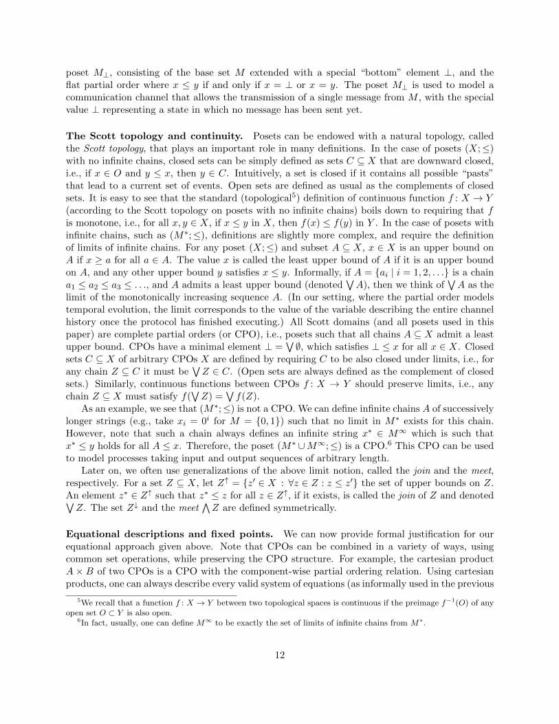
Sim(yA, sA) = (y′A, rA):rA[a] = sa[A] (a ∈ A)rA[h] = yA (h ∈ H)y′A = yA

Sim’(x′, w, yA, sA) = (x, rA, y′A):

uh = (x′ ∧ w[h]) ∨ t1(sA[h], uH) (h ∈ H)x = t2(sA[h], uH) (h = minH)y′a = x′ ∧ w[a] (a ∈ A)ra[A] = sA[a] (a ∈ A)ra[H] = uH (a ∈ A)

Figure 12: Simulators for the broadcast protocol when the dealer is honest (left) or dishonest (right)

WCast

Player[H]

Net

x′, w y′A

y′H

yH

sHrH

sArA

BCastSim

x′, w

x

y′ArA

sA

yA

yH

Figure 13: Security of broadcast protocol when the dealer is corrupted.

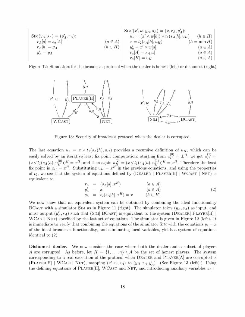
The last equation uh = x ∨ t1(sA(h), uH) provides a recursive definition of uH , which can be

easily solved by an iterative least fix point computation: starting from u(0)H = ⊥H , we get u

(1)H =

(x∨ t1(sA(h), u(0)H ))H = xH , and then again u

(2)H = (x∨ t1(sA(h), u

(1)H ))H = xH . Therefore the least

fix point is uH = xH . Substituting uH = xH in the previous equations, and using the propertiesof t2, we see that the system of equations defined by (Dealer | Player[H] | WCast | Net) isequivalent to

ra = (sA[a], xH) (a ∈ A)y′a = x (a ∈ A)yh = t2(sA[h], xH) = x (h ∈ H)

(2)

We now show that an equivalent system can be obtained by combining the ideal functionalityBCast with a simulator Sim as in Figure 11 (right). The simulator takes (yA, sA) as input, andmust output (y′A, rA) such that (Sim| BCast) is equivalent to the system (Dealer| Player[H] |WCast| Net) specified by the last set of equations. The simulator is given in Figure 12 (left). Itis immediate to verify that combining the equations of the simulator Sim with the equations yi = xof the ideal broadcast functionality, and eliminating local variables, yields a system of equationsidentical to (2).

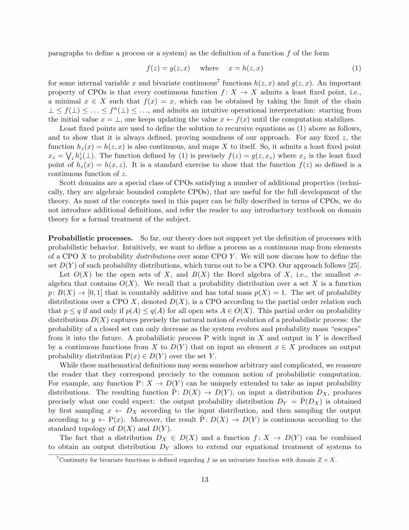
Dishonest dealer. We now consider the case where both the dealer and a subset of playersA are corrupted. As before, let H = {1, . . . , n} \ A be the set of honest players. The systemcorresponding to a real execution of the protocol when Dealer and Player[A] are corrupted is(Player[H] | WCast| Net), mapping (x′, w, sA) to (yH , rA, y

′A). (See Figure 13 (left).) Using

the defining equations of Player[H], WCast and Net, and introducing auxiliary variables uh =

18

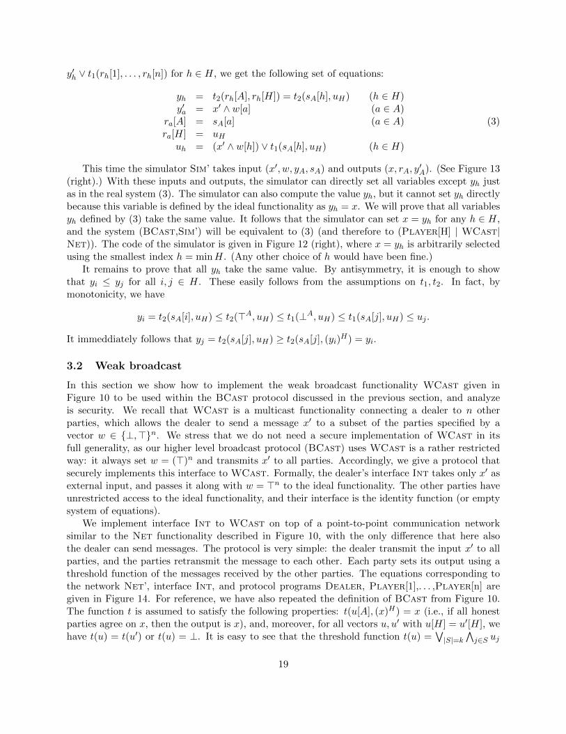
y′h ∨ t1(rh[1], . . . , rh[n]) for h ∈ H, we get the following set of equations:

yh = t2(rh[A], rh[H]) = t2(sA[h], uH) (h ∈ H)y′a = x′ ∧ w[a] (a ∈ A)

ra[A] = sA[a] (a ∈ A)ra[H] = uH

uh = (x′ ∧ w[h]) ∨ t1(sA[h], uH) (h ∈ H)

(3)

This time the simulator Sim’ takes input (x′, w, yA, sA) and outputs (x, rA, y′A). (See Figure 13

(right).) With these inputs and outputs, the simulator can directly set all variables except yh justas in the real system (3). The simulator can also compute the value yh, but it cannot set yh directlybecause this variable is defined by the ideal functionality as yh = x. We will prove that all variablesyh defined by (3) take the same value. It follows that the simulator can set x = yh for any h ∈ H,and the system (BCast,Sim’) will be equivalent to (3) (and therefore to (Player[H] | WCast|Net)). The code of the simulator is given in Figure 12 (right), where x = yh is arbitrarily selectedusing the smallest index h = minH. (Any other choice of h would have been fine.)

It remains to prove that all yh take the same value. By antisymmetry, it is enough to showthat yi ≤ yj for all i, j ∈ H. These easily follows from the assumptions on t1, t2. In fact, bymonotonicity, we have

yi = t2(sA[i], uH) ≤ t2(>A, uH) ≤ t1(⊥A, uH) ≤ t1(sA[j], uH) ≤ uj .

It immeddiately follows that yj = t2(sA[j], uH) ≥ t2(sA[j], (yi)H) = yi.

3.2 Weak broadcast

In this section we show how to implement the weak broadcast functionality WCast given inFigure 10 to be used within the BCast protocol discussed in the previous section, and analyzeis security. We recall that WCast is a multicast functionality connecting a dealer to n otherparties, which allows the dealer to send a message x′ to a subset of the parties specified by avector w ∈ {⊥,>}n. We stress that we do not need a secure implementation of WCast in itsfull generality, as our higher level broadcast protocol (BCast) uses WCast is a rather restrictedway: it always set w = (>)n and transmits x′ to all parties. Accordingly, we give a protocol thatsecurely implements this interface to WCast. Formally, the dealer’s interface Int takes only x′ asexternal input, and passes it along with w = >n to the ideal functionality. The other parties haveunrestricted access to the ideal functionality, and their interface is the identity function (or emptysystem of equations).

We implement interface Int to WCast on top of a point-to-point communication networksimilar to the Net functionality described in Figure 10, with the only difference that here alsothe dealer can send messages. The protocol is very simple: the dealer transmit the input x′ to allparties, and the parties retransmit the message to each other. Each party sets its output using athreshold function of the messages received by the other parties. The equations corresponding tothe network Net’, interface Int, and protocol programs Dealer, Player[1],. . . ,Player[n] aregiven in Figure 14. For reference, we have also repeated the definition of BCast from Figure 10.The function t is assumed to satisfy the following properties: t(u[A], (x)H) = x (i.e., if all honestparties agree on x, then the output is x), and, moreover, for all vectors u, u′ with u[H] = u′[H], wehave t(u) = t(u′) or t(u) = ⊥. It is easy to see that the threshold function t(u) =

∨|S|=k

∧j∈S uj

19

WCast(x′, w) = (y′1, . . . , y′n):

y′i = x′ ∧ w[i] (i = 1, . . . , n)

Int:w = >n

Net’(s′0, . . . , s′n) = (r′1, . . . , r

′n):

r′i[j] = s′j [i] (i = 1, . . . , n; j = 0, . . . , n)

Dealer(x′) = (s′0):s′0[i] = x′ (i = 1, . . . , n)

Player[i](r′i) = (y′i, s′i): (i = 1, . . . , n)

s′i[j] = r′i[0] (j = 1, . . . , n)y′i = t(r′i[1], . . . , r′i[n])

Figure 14: Weak broadcast protocol.

satisfies both properties for k ≥ n+|A|+12 . Namely, take any two vectors u, u′ with u[H] = u′[H],

assume that there exist sets S and S′ such that uj = x for all j ∈ S and u′j = y all j ∈ S′. Then,since |S ∩ S′ ∩H| ≥ 2k − n− |A| > 0, and hence x = y.

As usual, we consider two cases in the proof of security, depending on whether the dealer iscorrupted or not.

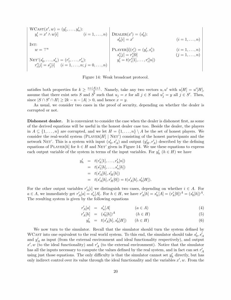
Dishonest dealer. It is convenient to consider the case when the dealer is dishonest first, as someof the derived equations will be useful in the honest dealer case too. Beside the dealer, the playersin A ⊆ {1, . . . , n} are corrupted, and we let H = {1, . . . , n} \ A be the set of honest players. Weconsider the real-world system (Player[H] | Net’) consisting of the honest partecipants and thenetwork Net’. This is a system with input (s′0, s

′A) and output (y′H , r

′A) described by the defining

equations of Player[h] for h ∈ H and Net’ given in Figure 14. We use these equations to expresseach output variable of the system in terms of the input variables. For y′h (h ∈ H) we have

y′h = t(r′h[1], . . . , r′h[n])

= t(s′1[h], . . . , s′n[h])

= t(s′A[h], s′H [h])

= t(s′A[h], r′H [0]) = t(s′A[h], s′0[H]).

For the other output variables r′A[i] we distinguish two cases, depending on whether i ∈ A. Fora ∈ A, we immediately get r′A[a] = s′a[A]. For h ∈ H, we have r′A[h] = s′h[A] = (r′h[0])A = (s′0[h])A.The resulting system is given by the following equations

r′A[a] = s′a[A] (a ∈ A) (4)

r′A[h] = (s′0[h])A (h ∈ H) (5)

y′h = t(s′A[h], s′0[H]) (h ∈ H) (6)

We now turn to the simulator. Recall that the simulator should turn the system defined byWCast into one equivalent to the real world system. To this end, the simulator should take s′0, s

′A

and y′A as input (from the external environment and ideal functionality respectively), and outputx′, w (to the ideal functionality) and r′A (to the external environment). Notice that the simulatorhas all the inputs necessary to compute the values defined by the real system, and in fact can set r′Ausing just those equations. The only difficulty is that the simulator cannot set y′h directly, but hasonly indirect control over its value through the ideal functionality and the variables x′, w. From the

20

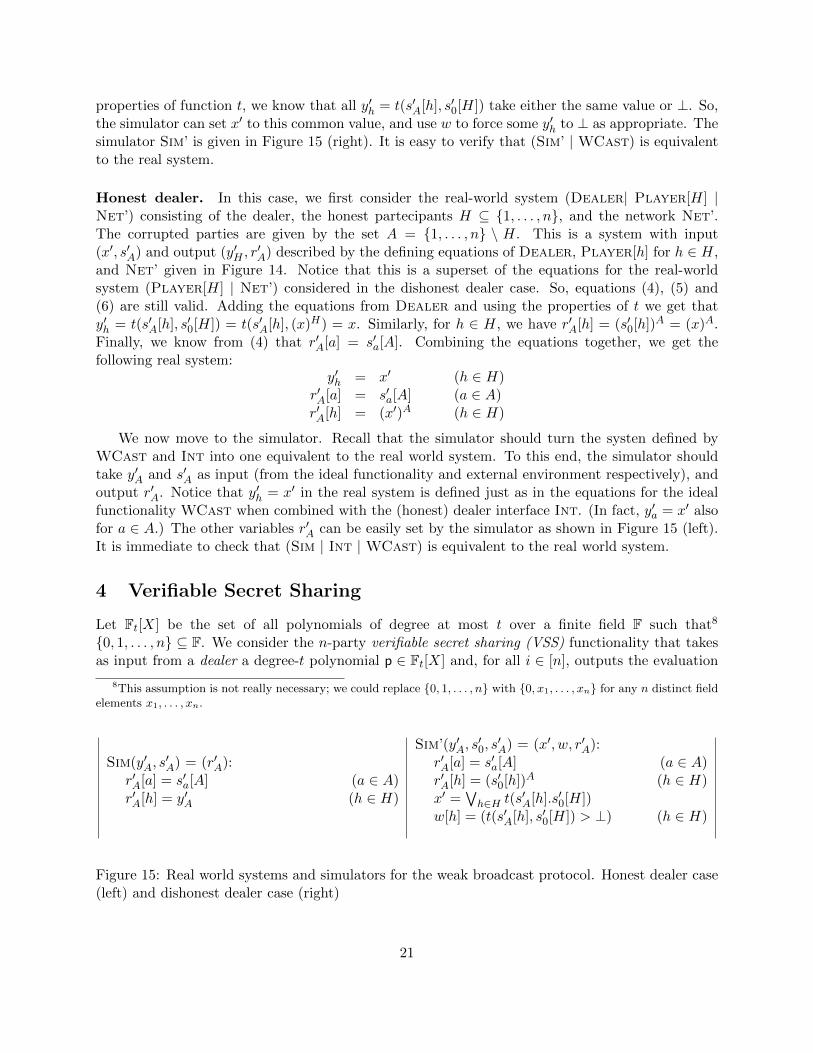
properties of function t, we know that all y′h = t(s′A[h], s′0[H]) take either the same value or ⊥. So,the simulator can set x′ to this common value, and use w to force some y′h to ⊥ as appropriate. Thesimulator Sim’ is given in Figure 15 (right). It is easy to verify that (Sim’ |WCast) is equivalentto the real system.

Honest dealer. In this case, we first consider the real-world system (Dealer| Player[H] |Net’) consisting of the dealer, the honest partecipants H ⊆ {1, . . . , n}, and the network Net’.The corrupted parties are given by the set A = {1, . . . , n} \ H. This is a system with input(x′, s′A) and output (y′H , r

′A) described by the defining equations of Dealer, Player[h] for h ∈ H,

and Net’ given in Figure 14. Notice that this is a superset of the equations for the real-worldsystem (Player[H] | Net’) considered in the dishonest dealer case. So, equations (4), (5) and(6) are still valid. Adding the equations from Dealer and using the properties of t we get thaty′h = t(s′A[h], s′0[H]) = t(s′A[h], (x)H) = x. Similarly, for h ∈ H, we have r′A[h] = (s′0[h])A = (x)A.Finally, we know from (4) that r′A[a] = s′a[A]. Combining the equations together, we get thefollowing real system:

y′h = x′ (h ∈ H)r′A[a] = s′a[A] (a ∈ A)r′A[h] = (x′)A (h ∈ H)

We now move to the simulator. Recall that the simulator should turn the systen defined byWCast and Int into one equivalent to the real world system. To this end, the simulator shouldtake y′A and s′A as input (from the ideal functionality and external environment respectively), andoutput r′A. Notice that y′h = x′ in the real system is defined just as in the equations for the idealfunctionality WCast when combined with the (honest) dealer interface Int. (In fact, y′a = x′ alsofor a ∈ A.) The other variables r′A can be easily set by the simulator as shown in Figure 15 (left).It is immediate to check that (Sim | Int | WCast) is equivalent to the real world system.

4 Verifiable Secret Sharing

Let Ft[X] be the set of all polynomials of degree at most t over a finite field F such that8

{0, 1, . . . , n} ⊆ F. We consider the n-party verifiable secret sharing (VSS) functionality that takesas input from a dealer a degree-t polynomial p ∈ Ft[X] and, for all i ∈ [n], outputs the evaluation

8This assumption is not really necessary; we could replace {0, 1, . . . , n} with {0, x1, . . . , xn} for any n distinct fieldelements x1, . . . , xn.

Sim(y′A, s′A) = (r′A):

r′A[a] = s′a[A] (a ∈ A)r′A[h] = y′A (h ∈ H)

Sim’(y′A, s′0, s′A) = (x′, w, r′A):

r′A[a] = s′a[A] (a ∈ A)r′A[h] = (s′0[h])A (h ∈ H)x′ =

∨h∈H t(s′A[h].s′0[H])

w[h] = (t(s′A[h], s′0[H]) > ⊥) (h ∈ H)

Figure 15: Real world systems and simulators for the weak broadcast protocol. Honest dealer case(left) and dishonest dealer case (right)

21

Player[H]Net’

y′H

s′H

r′H

s′0 r′As′A

Sim’ WCasty′A

x′, w

y′Hs′0s′A r′A

Figure 16: Security of the weak multicast protocol, when the dealer is dishonest. Real worldexecution on the left. Simulated attack in the ideal world on the right.

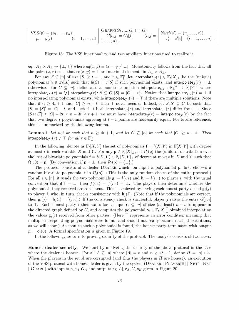
p(i) to the i-th party. The formal definition of VSS: Ft[X]⊥ 7→ Fn⊥ is given in Figure 18 (left),

where by convention ⊥(x) = ⊥ for all x.We devise a protocol implementing the VSS functionality on top of a point-to-point network

functionality Net defined as in the previous section that allows the n parties to exchange elementsfrom F, and two other auxiliary functionalities. The protocol is based on the one by [5]. Even thoughits complexity is exponential in n, we have chosen to present this protocol due to its simplicity.The first auxiliary functionality (Graph) grants all parties access to the adjacency matrix of ann-vertex directed graph (with loops), where each party i ∈ [n] can add outgoing edges to vertexi, but not to any other vertex j 6= i. Formally, Graph: {⊥,>}n × · · · × {⊥,>}n → {⊥,>}n×n isgiven in Figure 18 (center). Setting G[i, j] = > is interpreted as including an edge from i to j in thegraph. Graph can be immediately implemented using n copies of a broadcast functionality, wherea different party acts as the sender in each copy. We also assume the availability of an additionalunidirectional network functionality Net’ : (Ft[X]2⊥)n → (Ft[X]2⊥)n that allows the VSS dealer tosend to each party a pair of polynomials of degree at most t. See Figure 18 (right).

The VSS protocol. We turn to the actual protocol securely implementing the VSS functionality.We first define some auxiliary functions. For any subset C ⊆ [n], let cliqueC : {⊥,>}n×n → {⊥,>}be the function cliqueC(G) =

∧i,j∈C G[i, j]. This function is clearly monotone, and tests if C

is a clique in G. For any set A, we equip the set A⊥ with a monotone equality-test function

Player[H]Net’

Dealer

y′H

s′H

r′H

s′0

x′

r′As′A

Sim

Int

WCasty′A

wx′ y′Hs′A r′A

Figure 17: Security of the weak multicast protocol, when the dealer is honest. Real world executionon the left. Simulated attack in the ideal world on the right.

22

VSS(p) = (p1, . . . , pn)pi = p(i) (i = 1, . . . , n)

Graph(G1, ..., Gn) = G:G[i, j] = Gi[j] (i, j =

1, . . . , n) .

Net’(s′) = (r′1, . . . , r′n):

r′i = s′[i] (i = 1, . . . , n) .

Figure 18: The VSS functionality, and two auxiliary functions used to realize it.

eq : A⊥ ×A⊥ → {⊥,>} where eq(x, y) ≡ (x = y 6= ⊥). Monotonicity follows from the fact that allthe pairs (x, x) such that eq(x, y) = > are maximal elements in A⊥ ×A⊥.

For any S ⊆ [n] of size |S| ≥ t + 1, and r ∈ Fnb , let interpolateS(r) ∈ Ft[X]⊥ be the (unique)

polynomial h ∈ Ft[X] such that h(S) = r[S] if such polynomial exists, and interpolateS(r) = ⊥otherwise. For C ⊆ [n], define also a monotone function interpolateC,t : F⊥n → Ft[Y ]>⊥ whereinterpolateC,t(r) =

∨{interpolateS(r) : S ⊆ C, |S| = |C| − t}. Notice that interpolateC,t(r) = ⊥ if

no interpolating polynomial exists, while interpolateC,t(r) = > if there are multiple solutions. Notethat if n ≥ 4t + 1 and |C| ≥ n − t, then > never occurs: Indeed, let S, S′ ⊆ C be such that|S| = |S|′ = |C| − t, and such that both interpolateS(r) and interpolateS′(r) differ from ⊥. Since|S ∩ S′| ≥ |C| − 2t ≥ n − 3t ≥ t + 1, we must have interpolateS(r) = interpolateS′(r) by the factthat two degree t polynomials agreeing at t + 1 points are necessarily equal. For future reference,this is summarized by the following lemma.

Lemma 1 Let n, t be such that n ≥ 4t + 1, and let C ⊆ [n] be such that |C| ≥ n − t. TheninterpolateC,t(r) 6= > for all r ∈ Fn

⊥.

In the following, denote as Ft[X,Y ] the set of polynomials f = f(X,Y ) in F[X,Y ] with degreeat most t in each variable X and Y . For any p ∈ Ft[X]⊥, let Pt(p) the (uniform distribution overthe) set of bivariate polynomials f = f(X,Y ) ∈ Ft[X,Y ]⊥ of degree at most t in X and Y such thatf(·, 0) = p. (By convention, if p = ⊥, then Pt(p) = {⊥}.)

The protocol consists of a dealer Dealer which, on input a polynomial p, first chooses arandom bivariate polynomial f in Pt(p). (This is the only random choice of the entire protocol.)For all i ∈ [n], it sends the two polynomials gi = f(·, i) and hi = f(i, ·) to player i, with the usualconvention that if f = ⊥, then f(·, i) = f(i, ·) = ⊥. The players then determine whether thepolynomials they received are consistent. This is achieved by having each honest party i send gi(j)to player j, who, in turn, checks consistency with hj(i). (Note that if the polynomials are correct,then gi(j) = hj(i) = f(j, i).) If the consistency check is successful, player j raises the entry G[j, i]to >. Each honest party i then waits for a clique C ⊆ [n] of size (at least) n − t to appear inthe directed graph defined by G, and computes the polynomial oi ∈ Ft[X]>⊥ obtained interpolatingthe values gj(i) received from other parties. (Here > represents an error condition meaning thatmultiple interpolating polynomials were found, and should not really occur in actual executions,as we will show.) As soon as such a polynomial is found, the honest party terminates with outputpi = oi(0). A formal specification is given in Figure 19.

In the following, we turn to proving security of the protocol. The analysis consists of two cases.

Honest dealer security. We start by analyzing the security of the above protocol in the casewhere the dealer is honest. For all A ⊆ [n] where |A| = t and n ≥ 4t + 1, define H = [n] \ A.When the players in the set A are corrupted (and thus the players in H are honest), an executionof the VSS protocol with honest dealer is given by the system (Dealer | Player[H] | Net’ | Net| Graph) with inputs p, sA, GA and outputs rD[A], rA, G, pH given in Figure 20.

23

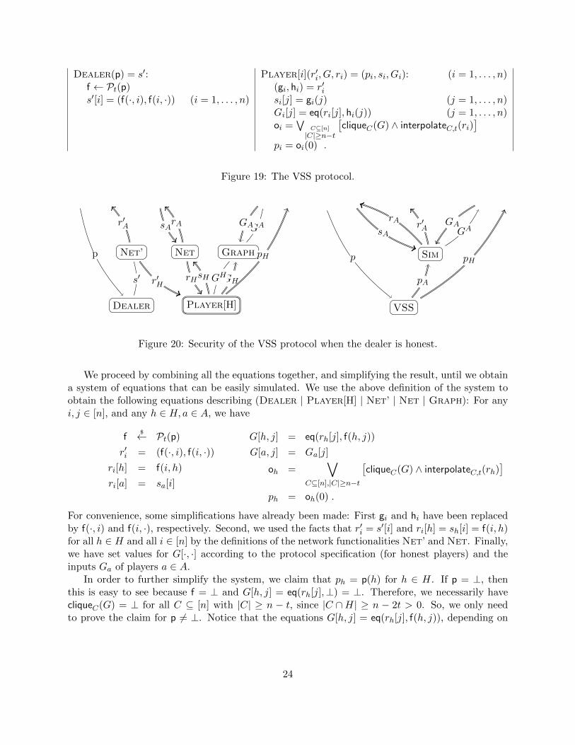
Dealer(p) = s′:f ← Pt(p)s′[i] = (f(·, i), f(i, ·)) (i = 1, . . . , n)

Player[i](r′i, G, ri) = (pi, si, Gi): (i = 1, . . . , n)(gi, hi) = r′isi[j] = gi(j) (j = 1, . . . , n)Gi[j] = eq(ri[j], hi(j)) (j = 1, . . . , n)oi =

∨C⊆[n]

|C|≥n−t

[cliqueC(G) ∧ interpolateC,t(ri)

]pi = oi(0) .

Figure 19: The VSS protocol.

Dealer

Net’

Player[H]

GraphNetp

s′

r′A

r′H GH

pH

sHrH GH

GAGArAsA

VSS

Sim

pA

p pH

r′A GAGA

rAsA

Figure 20: Security of the VSS protocol when the dealer is honest.

We proceed by combining all the equations together, and simplifying the result, until we obtaina system of equations that can be easily simulated. We use the above definition of the system toobtain the following equations describing (Dealer | Player[H] | Net’ | Net | Graph): For anyi, j ∈ [n], and any h ∈ H, a ∈ A, we have

f$← Pt(p)

r′i = (f(·, i), f(i, ·))ri[h] = f(i, h)

ri[a] = sa[i]

G[h, j] = eq(rh[j], f(h, j))

G[a, j] = Ga[j]

oh =∨

C⊆[n],|C|≥n−t

[cliqueC(G) ∧ interpolateC,t(rh)

]ph = oh(0) .

For convenience, some simplifications have already been made: First gi and hi have been replacedby f(·, i) and f(i, ·), respectively. Second, we used the facts that r′i = s′[i] and ri[h] = sh[i] = f(i, h)for all h ∈ H and all i ∈ [n] by the definitions of the network functionalities Net’ and Net. Finally,we have set values for G[·, ·] according to the protocol specification (for honest players) and theinputs Ga of players a ∈ A.

In order to further simplify the system, we claim that ph = p(h) for h ∈ H. If p = ⊥, thenthis is easy to see because f = ⊥ and G[h, j] = eq(rh[j],⊥) = ⊥. Therefore, we necessarily havecliqueC(G) = ⊥ for all C ⊆ [n] with |C| ≥ n − t, since |C ∩H| ≥ n − 2t > 0. So, we only needto prove the claim for p 6= ⊥. Notice that the equations G[h, j] = eq(rh[j], f(h, j)), depending on

24

whether j = h′ ∈ H or j = a ∈ A, can be replaced by the set of equations

G[h, h′] = eq(rh[h′], f(h, h′)) = eq(f(h, h′), f(h, h′)) = >G[h, a] = eq(rh[a], f(h, a)) = eq(sa[h], f(h, a)) .

This in particular implies that C = H is a clique of size at least n − t in the graph defined by G,i.e., we have cliqueH(G) = > by the above. Also, since rh[h′] = f(h, h′), we necessarily have

oh ≥ cliqueH(G) ∧ interpolateH,t(rh) = > ∧ f(h, ·) = f(h, ·)

by Lemma 1. Now, let S ⊆ C be any sets such that |C| ≥ n− t and |S| = |C| − t ≥ n− 2t. Sinceoh(h′) = f(h, h′) for all h′ ∈ H and |S ∩H| ≥ n − 3t ≥ t + 1, we have interpolateS(rh) ≥ f(h, ·),and, by Lemma 1, interpolateS(rh) = f(h, ·). This proves that oh = interpolateC,t(rh) = f(h, ·), andph = oh(0) = f(h, 0) = p(h).

Summarizing, the real system is described by the following set of equations:

f$← Pt(p)

r′a = (f(·, a), f(a, ·))ra[a′] = sa′ [a]

ra[h] = f(a, h)

G[h, h′] = (p > ⊥)

G[h, a] = eq(sa[h], f(h, a))

G[a, j] = Ga[j]

ph = p(h) .

Notice that this is exactly how ph is defined by the VSS functionality. So, in order to prove security,it is enough to give a simulator Sim that on input pA, sA, GA, outputs G, rA and r′A as defined inthe above system of equations. See Figure 20 (right).

The problem faced by the simulator is that it cannot test p > ⊥ and generate f as in the equationsbecause it does not know the value of p, rather it only has partial information pA = p(A). Thefirst condition p > ⊥ is easy to check because it is equivalent to pa = p(a) > ⊥ for any a ∈ A. Inorder to complete the simulation, we observe that the equations only depend on the 2t polynomialsf(·, A) and f(A, ·). The next lemma shows that, given p(A), the polynomials f(·, A) and f(A, ·) arestatistically independent from p, and their distribution can be easily sampled.

Lemma 2 Let p ∈ Ft[X], let f$← Pt(p), and for all a ∈ A, let ga = f(·, a) and ha = f(a, ·). The

conditional distribution of (ga, ha)a∈A given p(A) is statistically independent of p, and it can begenerated by the following algorithm Samp(pA): first pick random polynomials ha ∈ Ft[Y ] indepen-dently and uniformly at random subject to the constraint ha(0) = pa. Then, pick ga ∈ Ft[X], alsoindependently and uniformly at random, subject to the constraint ga(A) = hA(a).

Using the algorithm from the lemma, we obtain the following simulator Sim:

Sim(pA, sA, GA) = (GA, rA, r′A):(gA, hA)← Samp(pA)r′A = (gA, hA)ra[h] = ha(h) (h ∈ H, a ∈ A)ra[a′] = sa′ [a] (a, a′ ∈ A)

G[h, h′] =∨

a∈A(pa > ⊥) (h, h′ ∈ H)G[h, a] = eq(sa[h], ga(h)) (h ∈ H, a ∈ A)G[a, j] = Ga[j] (a ∈ A, j ∈ [n])

As usual, if p = ⊥, then pA = ⊥A and by convention Samp(pA) = {⊥,⊥}.

25

Dishonest dealer security. We now look at the case where the dealer is not honest. As above,for all A ⊆ [n] where |A| = t and n ≥ 4t + 1, define H = [n] \ A. When the players in the setA are corrupted (and thus the players in H are honest), an execution of the VSS protocol withdishonest dealer is given by the system (Player[H] | Net’ | Net | Graph) with inputs s′, rA, GA,and outputs r′A, sA, pH and GA. As above, we start with an equational description of the system,and will simplify it below into a form where the construction of a corresponding simulator becomesobvious. For all i, j ∈ [n], h, h′ ∈ H, and a ∈ A, we have

(gh, hh) = s′[h]

r′a = s′[a]

ri[h] = gh(i)

ri[a] = sa[i]

G[h, h′] = eq(gh′(h), hh(h′))

G[h, a] = eq(sa[h], hh(a))

G[a, j] = Ga[j]

oh =∨

C⊆[n],|C|≥n−t

[cliqueC(G) ∧ interpolateC,t(rh)

]ph = oh(0) .

Notice that we have already undertaken several easy simplification steps, defining variables whichare part of the output as a function of the system inputs and of auxiliary variables gH , hH , oH ,and rH . Specifically, to obtain the above equations starting from the original system specification,we have used ri[j] = sj [i], where sh[i] = gh(i), together with r′i = s′[i] and the definition of G[h, i],distinguishing between the cases i = a ∈ A and i = h′ ∈ H.

Recall that in order to prove security, we need to give a simulator Sim with input s′, GA, sA, pAand output r′A, rA, G

A and p such that (VSS | Sim) is equivalent to the above system. (SeeFigure 21.) Notice that in the system describing a real execution, all variables except ph (andintermediate value oh) are defined as functions of the inputs given to the simulator. So, Sim can setall these variables just as in the system describing the real execution. The only difference betweena real execution and a simulation is that the simulator is not allowed to set ph directly. Rather, itshould specify a polynomial p ∈ Ft[X]⊥, which implicitly defines ph = p(h) through the equationsof the ideal VSS functionality. In other words, in order to complete the description of the simulatorwe need to show that Sim can determine such a polynomial p based on its inputs s′, GA, sA, pAsuch that p(h) equals ph as defined by the above system of equations.

Before defining p, we recall the following lemma whose simple proof is standard and omitted:

Lemma 3 Let S be such that |S| ≥ t+1 and let {gh, hh}h∈S be a set of 2 · |S| polynomials of degreet. Then, gh(h′) = hh′(h) for all h, h′ ∈ S holds if and only if there exists a unique polynomialf ∈ Ft[X,Y ] such that f(·, h) = gh and f(h, ·) = hh for all h ∈ S.

For T ⊆ H, |T | ≥ t+ 1, define interpolate2T (s′) to be the (unique) polynomial f ∈ Ft[X,Y ] suchthat f(·, h) = gh and f(h, ·) = hh for all h ∈ T (if it exists), and ⊥ otherwise or if s′[h] = ⊥ for someh ∈ T . Also, given C ⊆ [n], define

interpolate2C(s′) =∨{interpolate2S(s′) : S ⊆ C, |S| ≥ |C| − t} .

Note that since |C| ≥ n − t and n ≥ 4t + 1, interpolate2C(s′) 6= >. Indeed, for any two S, S′ ⊆ Csuch that both interpolate2S(s′) and interpolate2S′(s

′) differ from ⊥, we have |S ∩ S′| ≥ t + 1 andhence interpolate2S(s′) = interpolate2S∩S′(s

′) = interpolate2S′(s′) by Lemma 3. We finally define

the polynomial p = f(·, 0), where

f =∨

C⊆[n],|C|≥n−t

cliqueC(G) ∧ interpolate2C(s′) . (7)

26

Net’

Player[H]

GraphNet

s′ r′A

r′HGH

pH

sHrH GH

GAGArAsA

VSS

Sim

pAp

pH

r′As′

GA

GA

rAsA

Figure 21: Security of the VSS protocol when the dealer is dishonest.

We first prove that p < >: To this end, assume that p 6= ⊥. Then, f 6= ⊥, and there must existC ⊆ [n] such that cliqueC(G) = >. Let S = C ∩H. Note that for all h, h′ ∈ S, since G[h, h′] = >,it must be that hh(h′) = gh′(h). Therefore, since |S| ≥ n− 2t > 2t+ 1, by Lemma 3, there exists aunique polynomial fC such that f(·, h) = gh and f(h, ·) = hh for all h ∈ S, and by the above

fC = interpolate2C(s′) = interpolate2C∩H(s′) .

Now assume that there exist two such cliques C and C ′, with S = C ∩H and S′ = C ′ ∩H. Then,since ∣∣S ∩ S′∣∣ = |S|+

∣∣S′∣∣− ∣∣S ∪ S′∣∣ ≥ 2(|C| − |A|)− |H| ≥ n− 3 |A| ≥ t+ 1 , (8)

by Lemma 3, we necessarily have fC = fC′ = f.Finally, it is easy to see that p(h) = ph for all h ∈ H. Namely, if there exists C ⊆ [n]

with cliqueC(G) = >, then rh[h′] = gh′(h) = f(h, h′) for all h′ ∈ C ∩ H, and therefore oh =interpolateC(rh) = interpolateC∩H(rh) = f(h, ·), and thus ph = oh(0) = f(h, 0) = p(h).

We therefore conclude that the real system is equivalent to (Sim| VSS) where Sim is thesimulator defined by the following equations:

Sim(s′, GA, sA, pA) = (r′A, rA, GA, p):

r′a = s′[a] (a ∈ A)ra[h] = gh(a) (h ∈ H, a ∈ A)ra[a′] = sa′ [a] (a, a′ ∈ A)G[h, h′] = eq(gh′(h), hh(h′)) (h, h′ ∈ H)

G[h, a] = eq(sa[h], hh(a)) (a ∈ A, h ∈ H)G[a, j] = Ga[j] (a ∈ A, j ∈ [n])f =

∨C⊆[n]

|C|≥n−tcliqueC(G) ∧ interpolate2C(s′)

p = f(·, 0)

5 Conclusions

Recognizing the inherent hardness of delivering security proofs for complex cryptographic protocolsthat are both precise and intuitive within existing security frameworks, we have presented a newframework to study the security of multi-party computations based on equational descriptionsof interactive processes. Our framework allows a simple and intuitive, yet completely formal,description of interactive processes via sets of equations, and its foundations rely on tools fromprogramming-language theory and domain theory. Beyond its simplicity, our framework completely

27

avoids explicit addressing of non-determinism within cryptographic security proofs, making securityproofs a matter of simple equational manipulations over precise mathematical structures. As acase study, we have presented simple security analyses of (variants of) two classical asynchronousprotocols within our framework, Bracha’s broadcast protocol [8] and the Ben-Or, Canetti, GoldreichVSS protocol [5].

We are convinced that our work will open up the avenue to several directions for future work.First off, while the results in this paper are presented for the special case of perfect security, a naturalnext step is to extend the framework to statistical and even computational security. Moreover, whilethe expressiveness of our framework (i.e., the monotonicity restrictions on protocols) remains tobe thoroughly investigated, most distributed protocols we examined so far, seemed to admit arepresentation within our framework, possibly after minor modifications which often resulted in asimpler protocol description. For this reason, our thesis is that this holds true for all protocolsof interest, and that non-monotonicity, as a source of unnecessary complexity and proof mistakes,should be avoided whenever possible.

References

[1] S. Abramsky and A. Jung. Handbook of Logic in Computer Science, volume III, chapterDomain theory, pages 1–168. Oxford University Press, 1994.

[2] Michael Backes, Birgit Pfitzmann, and Michael Waidner. A general composition theorem forsecure reactive systems. In TCC 2004, volume 2951 of Lecture Notes in Computer Science,pages 336–354, 2004.

[3] Donald Beaver and Shafi Goldwasser. Multiparty computation with faulty majority. InCRYPTO ’89, volume 435 of Lecture Notes in Computer Science, pages 589–590, 1989.

[4] Assaf Ben-David, Noam Nisan, and Benny Pinkas. FairplayMP: a system for secure multi-party computation. In ACM Conference on Computer and Communications Security, pages257–266, 2008.

[5] Michael Ben-Or, Ran Canetti, and Oded Goldreich. Asynchronous secure computation. InSTOC, pages 52–61, 1993.

[6] Michael Ben-Or, Shafi Goldwasser, and Avi Wigderson. Completeness theorems for non-cryptographic fault-tolerant distributed computation (extended abstract). In STOC ’88, pages1–10, 1988.

[7] Peter Bogetoft, Dan Lund Christensen, Ivan Damgard, Martin Geisler, Thomas P. Jakob-sen, Mikkel Krøigaard, Janus Dam Nielsen, Jesper Buus Nielsen, Kurt Nielsen, Jakob Pagter,Michael I. Schwartzbach, and Tomas Toft. Secure multiparty computation goes live. In Fi-nancial Cryptography (FC 2009), volume 5628 of Lecture Notes in Computer Science, pages325–343, 2009.

[8] Gabriel Bracha. An asynchronous [(n-1)/3]-resilient consensus protocol. In PODC ’84, pages154–162, 1984.

[9] Ran Canetti. Security and composition of multiparty cryptographic protocols. J. Cryptology,13(1):143–202, 2000.

28

[10] Ran Canetti. Universally composable security: A new paradigm for cryptographic protocols.In FOCS ’01, pages 136–145, 2001.

[11] Ivan Damgard, Marcel Keller, E. Larraia, C. Miles, and Nigel P. Smart. Implementing aes viaan actively/covertly secure dishonest-majority mpc protocol. IACR Cryptology ePrint Archive,2012.

[12] Oded Goldreich, Silvio Micali, and Avi Wigderson. How to play any mental game or a com-pleteness theorem for protocols with honest majority. In STOC ’87, pages 218–229, 1987.

[13] Shafi Goldwasser, Silvio Micali, and Charles Rackoff. The knowledge complexity of interactiveproof systems. SIAM J. Comput., 18(1):186–208, 1989.

[14] Carl A. Gunter. Semantics of programming languages - structures and techniques. Foundationsof computing. MIT Press, 1993.

[15] Dennis Hofheinz and Victor Shoup. Gnuc: A new universal composability framework. IACRCryptology ePrint Archive, 2011.

[16] G. Kahn. The semantics of a simple language for parallel programming. In J. L. Rosenfeld,editor, Information processing, pages 471–475, Stockholm, Sweden, Aug 1974. North Holland,Amsterdam.

[17] Vladimir Kolesnikov and Thomas Schneider. A practical universal circuit construction andsecure evaluation of private functions. In Financial Cryptography (FS 2008), volume 5143 ofLecture Notes in Computer Science, pages 83–97, 2008.

[18] Ralf Kusters. Simulation-based security with inexhaustible interactive turing machines. In 19thIEEE Computer Security Foundations Workshop, (CSFW-19 2006), pages 309–320, 2006.

[19] Dahlia Malkhi, Noam Nisan, Benny Pinkas, and Yaron Sella. Fairplay - secure two-partycomputation system. In USENIX Security Symposium, pages 287–302, 2004.

[20] Ueli Maurer and Renato Renner. Abstract cryptography. In Innovations in Computer Science- ICS 2010, pages 1–21, 2011.

[21] Ueli M. Maurer. Indistinguishability of random systems. In EUROCRYPT 2002, volume 2332of Lecture Notes in Computer Science, pages 110–132, 2002.

[22] Silvio Micali and Phillip Rogaway. Secure computation (abstract). In CRYPTO ’91, volume576 of Lecture Notes in Computer Science, pages 392–404, 1991.

[23] Birgit Pfitzmann and Michael Waidner. A model for asynchronous reactive systems and itsapplication to secure message transmission. In IEEE Symposium on Security and Privacy,pages 184–, 2001.

[24] Benny Pinkas, Thomas Schneider, Nigel P. Smart, and Stephen C. Williams. Secure two-partycomputation is practical. In ASIACRYPT 2009, volume 5912 of Lecture Notes in ComputerScience, pages 250–267, 2009.

29

[25] N. Saheb-Djahromi. Cpo’s of measures for nondeterminism. Theor. Comput. Sci., 12:19–37,1980.

[26] D. A. Schmidt. Denotational Semantics. Allyn and Bacon, 1986.

[27] J. E. Stoy. Denotational Semantics: The Scott-Strachey Approach to Programming LanguageTheory. MIT Press, 1977.

[28] Glynn Winskel. The formal semantics of programming languages - an introduction. Foundationof computing series. MIT Press, 1993.

[29] Andrew Chi-Chih Yao. Protocols for secure computations (extended abstract). In FOCS ’82,pages 160–164, 1982.

30